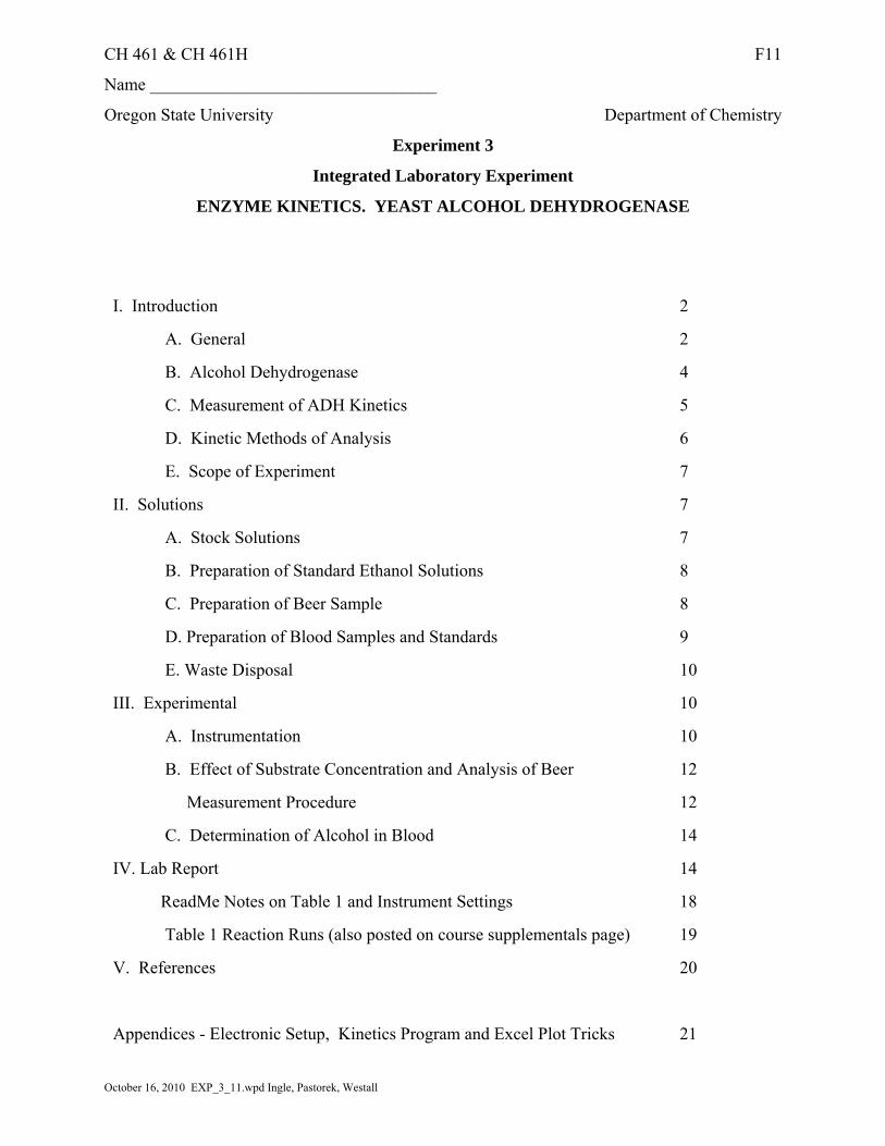
October 16, 2010 EXP_3_11.wpd Ingle, Pastorek, Westall

CH 461 & CH 461H F11

Name _________________________________

Oregon State University Department of Chemistry

Experiment 3

Integrated Laboratory Experiment

ENZYME KINETICS. YEAST ALCOHOL DEHYDROGENASE

I. Introduction 2

A. General 2

B. Alcohol Dehydrogenase 4

C. Measurement of ADH Kinetics 5

D. Kinetic Methods of Analysis 6

E. Scope of Experiment 7

II. Solutions 7

A. Stock Solutions 7

B. Preparation of Standard Ethanol Solutions 8

C. Preparation of Beer Sample 8

D. Preparation of Blood Samples and Standards 9

E. Waste Disposal 10

III. Experimental 10

A. Instrumentation 10

B. Effect of Substrate Concentration and Analysis of Beer 12

Measurement Procedure 12

C. Determination of Alcohol in Blood 14

IV. Lab Report 14

ReadMe Notes on Table 1 and Instrument Settings 18

Table 1 Reaction Runs (also posted on course supplementals page) 19

V. References 20

Appendices - Electronic Setup, Kinetics Program and Excel Plot Tricks 21

CH 461 & CH 461H F ‘112

k 2k -1

1kP + EE + S E S

[E]0v0

k2=

[S]0[S]0Km +

I. INTRODUCTION

A. General

Enzymes are an important class of proteins because they function as biological catalysts

which enable many essential chemical reactions to take place in living organisms. Enzyme

names are formed from a root indicating the substrate and the type of reaction and the suffix -

ase. Thus, "carbonic anhydrase" is an enzyme which catalyzes the reaction H2O + CO2 º

H2CO3. Enzymes can influence the rates of reactions considerably and can show

extraordinary selectivities with respect to substrates. Measurement of the rate of an enzyme

catalyzed reaction is the basis for some important analytical techniques for determination of

substrates, activators, inhibitors and enzymes. These determinations are often used for clinical

or diagnostic purposes.

The basic formulation for enzyme kinetics was developed by Michaelis and Menten. For

more detailed information about the formulation, refer to one of the general references given at

the end of this document. The theory is based on the following mechanism:

(1)

where E is the enzyme, S is the substrate, and P is the product, and ECS is an intermediate

enzyme-substrate complex and the k’s are rate constants for the respective steps in the

mechanism. If the steady state approximation applies to the enzyme-substrate complex, then it

can be shown that the initial steady state rate, or v0 = d [P] / d t, is given by

(2)

where Km = (k-1 + k2) / k-1 is the Michaelis-Menten constant,

[E]0 = initial enzyme molar concentration and

[S]0 = initial substrate molar concentration

The units of v0 are mol L-1s-1, of k2 and k-1 are s-1, of k1 are L mol-1s-1, and of Km are mol L-1.

CH 461 & CH 461H F ‘113

0.00

0.05

0.10

0.15

0.20

0.25

0 50 100 150 200

[S]0/mM

v 0/m

M/m

in

[S]0 << Km

[S]0 >> Km

==v0 vmax k2[E]0

v0 =[S]0[S]0Km +

vmax

v0 = [E]0[S]0 [S]0k2 Km( ) = Km( )vmax

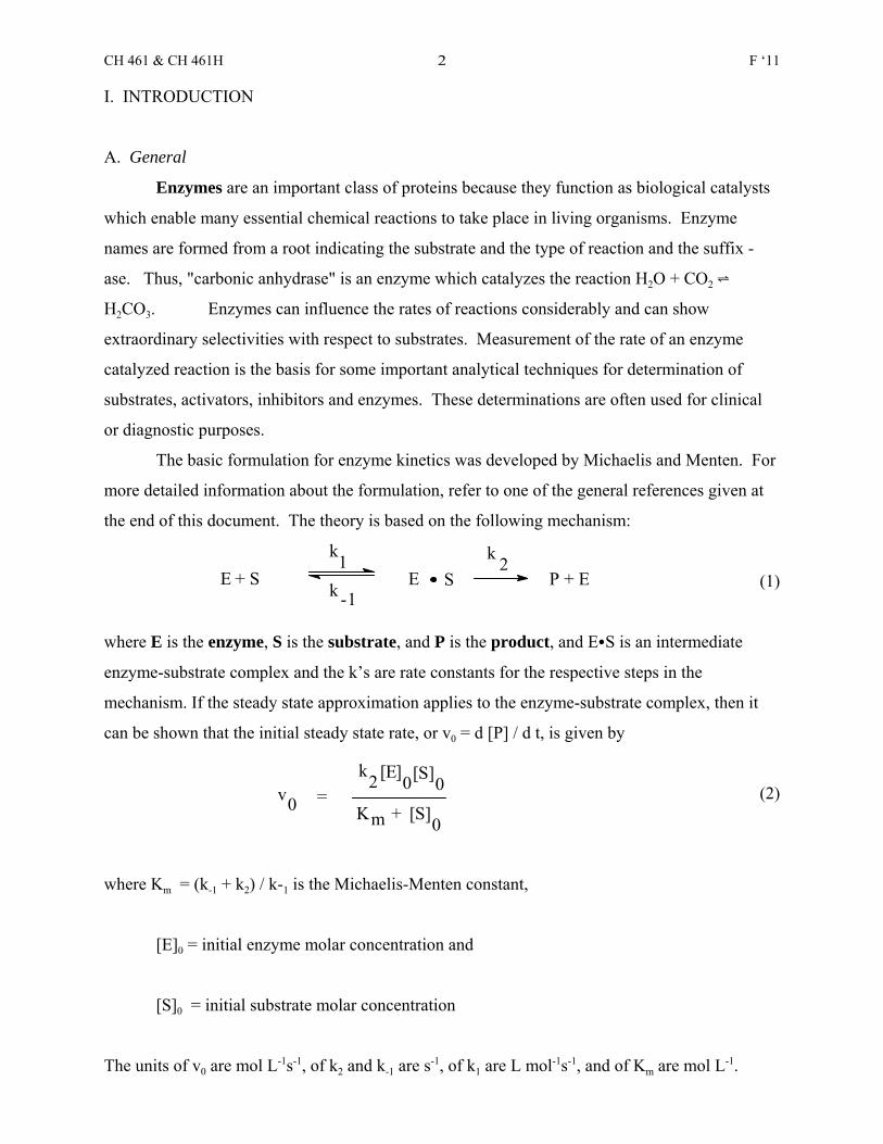
A plot of v0 versus [S]0 is shown in Figure 1.

Figure 1. Dependence of the initial rate on substrate concentration, according to equation 5.

Note that two regions in Figure 1 and equation 2 can be identified. At high substrate

concentrations, when [S]0 >> Km, v0 is independent of [S]0 and pseudo-zero order, and equation

2 reduces to

(3)

In this case, essentially all the enzyme present is bound with substrate in the ECS complex. At

low substrate concentration, when [S]0 << Km, the rate is linear in [S]0 or first order with respect

to [S]0, and equation 2 reduces to

(4)

The definition of vmax in equation 3 can be used to simplify equation 2 further.

Substitution of vmax (eq. 3) for k2[E]0 (eq. 2) yields the familiar two-parameter Michaelis-Menten

equation that is the basis for this experiment:

(5)

Equation 5 shows the experimentally observable v0 as a function of the initial substrate

concentration [S]0 and the two parameters vmax and Km. If experimental data for v0 and [S]0 are

available and plotted as in Figure 1, the value of vmax can be determined directly as the plateau

value of v0, and the value of Km can be determined from the fact that, according to equation 5,

CH 461 & CH 461H F ‘114

v0 = + vmax[S]0

Kmv0_

Km = [S]0 when vo = ½ vmax.

Alternatively, equation 5 can be transformed algebraically into a form that allows Km and

vmax to be determined through linear regression:

(6)

A plot of v0 vs. v0 /[S]0 (an Eadie-Hofstee plot) provides a simple means to find Km from the

slope and vmax from the intercept.

The mechanism of enzyme kinetic reactions is often much more complex than indicated

by equation 1 because two or more substrates, enzyme-substrate intermediates, or products may

be involved in the reaction. Nevertheless, it is experimentally found that many reactions obey

the Michaelis-Menten rate law indicated in equation 2 or 5 and that the determination of the

constants in those equations under a specified set of conditions provides a useful starting point

for characterization of enzyme catalyzed reactions.

B. Alcohol Dehydrogenase

The enzyme alcohol dehydrogenase (ADH) catalyzes the oxidation of ethanol to

acetaldehyde. The oxidizing agent, called a coenzyme, is nicotinamide adenine dinucleotide

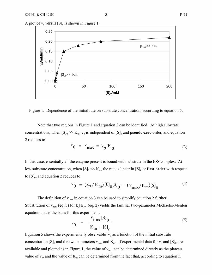
(NAD+, coenzyme I, diphosphopyridine nucleotide, DPN). Although, as shown in Figure 2, the

structure NAD+ is relatively complex, the reduction takes place only in the pyridine ring, as

shown in Figure 3. The oxidation of ethanol with NAD+ does not proceed at a measurable rate

unless the enzyme is present.

Alcohol dehydrogenase, which is isolated from yeast, is composed of more than 18

different amino acids, has a molecular weight of 1.5 x 105 and has four independent catalytic

sites. Zn2+ is present in amounts stoichiometric to the number of catalytic sites. Alcohol

dehydrogenase will catalyze the oxidation of a number of primary and secondary alcohols, but

not those in which there is halogen or amino substitution "- to the hydroxyl group.

An enzyme activity unit is often defined as the amount of enzyme that causes

transformation of one micromole of substrate per minute at 25°C under specified measurement

conditions. Enzymatic activity is usually measured under conditions where the amount of

enzyme is the rate limiting factor (i.e., equation 3, substrate and cofactor concentrations large

enough to be non-limiting). The specific activity is the number of enzyme units per mg of

CH 461 & CH 461H F ‘115

+O

+ CH3CH + H

(NADH)

(NAD+)

C

O

NH2

HH

R

Ndehydrogenase

alcoholCH3CH2OH+NH2

O

C

R

+N

protein and provides an indication of a relative purity. For example, the crystalline ADH that we

buy for this experiment usually contains between 300 to 400 units per mg, or equivalently, one

milligram of the ADH will convert 300 to 400 micromoles of substrate per minute.

Figure 2. Nicotinamide adenine dinucleotide (NAD +) (C21H27N7O14P2•4H2O, MW 735.5). Thepositive sign on NAD+ does not refer to the charge on the entire molecule but rather to the chargeon the pyridine ring.

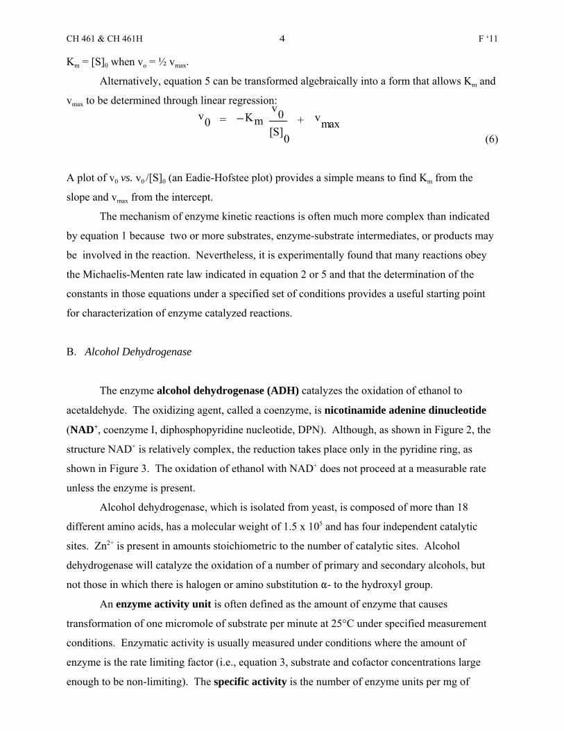
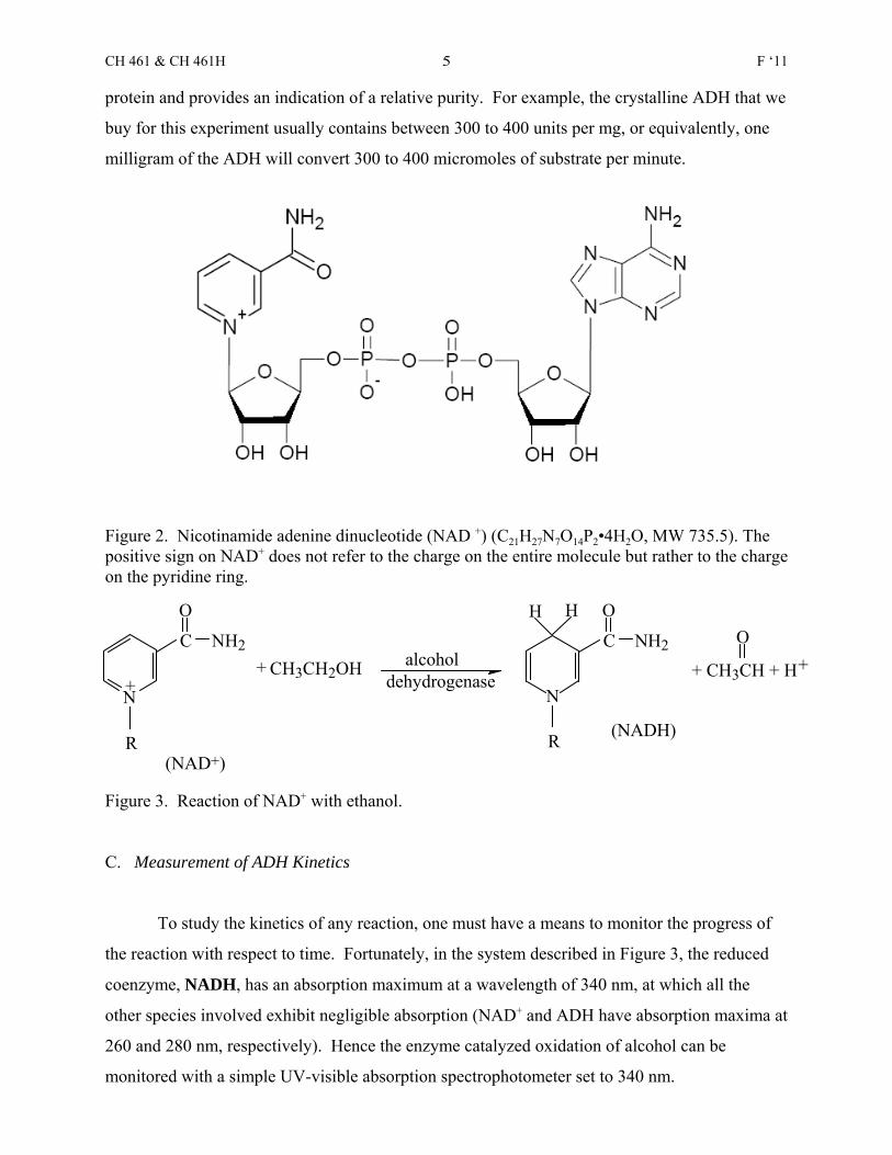
Figure 3. Reaction of NAD+ with ethanol.

C. Measurement of ADH Kinetics

To study the kinetics of any reaction, one must have a means to monitor the progress of

the reaction with respect to time. Fortunately, in the system described in Figure 3, the reduced

coenzyme, NADH, has an absorption maximum at a wavelength of 340 nm, at which all the

other species involved exhibit negligible absorption (NAD+ and ADH have absorption maxima at

260 and 280 nm, respectively). Hence the enzyme catalyzed oxidation of alcohol can be

monitored with a simple UV-visible absorption spectrophotometer set to 340 nm.

CH 461 & CH 461H F ‘116

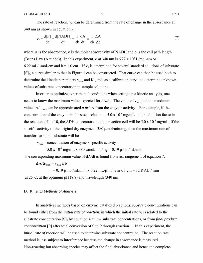
The rate of reaction, v0, can be determined from the rate of change in the absorbance at

340 nm as shown in equation 7:

(7)0

d[P] d[NADH] 1 dA 1 ΔAv = = =dt dt εb dt εb Δt

=

where A is the absorbance, , is the molar absorptivity of NADH and b is the cell path length

(Beer's Law (A = ,bc)). In this experiment, , at 340 nm is 6.22 x 103 L/mol-cm or

6.22 mL/:mol-cm and b = 1.0 cm. If v0 is determined for several standard solutions of substrate

[S]0, a curve similar to that in Figure 1 can be constructed. That curve can then be used both to

determine the kinetic parameters vmax and Km and, as a calibration curve, to determine unknown

values of substrate concentration in sample solutions.

In order to optimize experimental conditions when setting up a kinetic analysis, one

needs to know the maximum value expected for dA/dt. The value of vmax and the maximum

value dA/dtmax can be approximated a priori from the enzyme activity. For example, if the

concentration of the enzyme in the stock solution is 5.0 x 10-3 mg/mL and the dilution factor in

the reaction cell is 10, the ADH concentration in the reaction cell will be 5.0 x 10-4 mg/mL. If the

specific activity of the original dry enzyme is 380 :mol/min/mg, then the maximum rate of

transformation of substrate will be

vmax = concentration of enzyme x specific activity

= 5.0 x 10-4 mg/mL x 380 :mol/min/mg = 0.19 :mol/mL/min.

The corresponding maximum value of dA/dt is found from rearrangement of equation 7:

)A/)tmax = vmax , b

= 0.19 :mol/mL/min x 6.22 mL/:mol-cm x 1 cm = 1.18 AU / min

at 25°C, at the optimum pH (8.8) and wavelength (340 nm).

D. Kinetics Methods of Analysis

In analytical methods based on enzyme catalyzed reactions, substrate concentrations can

be found either from the initial rate of reaction, in which the initial rate v0 is related to the

substrate concentration [S]0 by equation 4 at low substrate concentrations, or from final product

concentration [P] after total conversion of S to P through reaction 1. In this experiment, the

initial rate of reaction will be used to determine substrate concentration. The reaction rate

method is less subject to interference because the change in absorbance is measured.

Non-reacting but absorbing species may affect the final absorbance and hence the complete-

CH 461 & CH 461H F ‘117

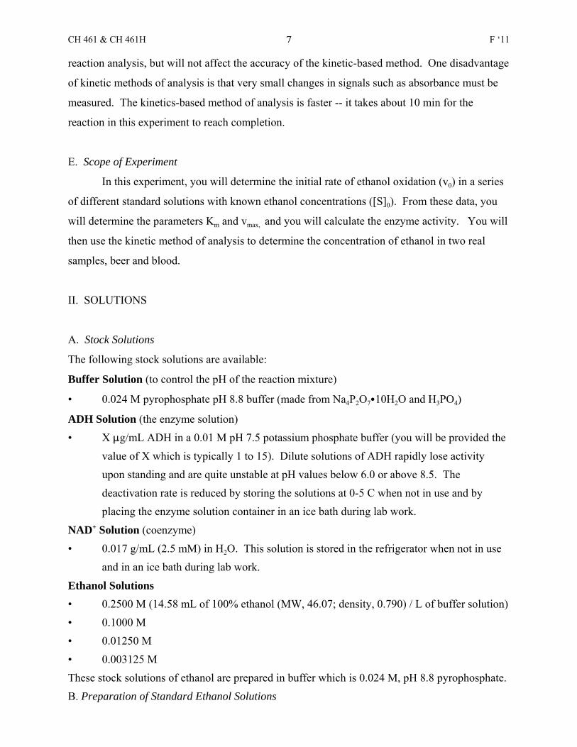
reaction analysis, but will not affect the accuracy of the kinetic-based method. One disadvantage

of kinetic methods of analysis is that very small changes in signals such as absorbance must be

measured. The kinetics-based method of analysis is faster -- it takes about 10 min for the

reaction in this experiment to reach completion.

E. Scope of Experiment

In this experiment, you will determine the initial rate of ethanol oxidation (v0) in a series

of different standard solutions with known ethanol concentrations ([S]0). From these data, you

will determine the parameters Km and vmax, and you will calculate the enzyme activity. You will

then use the kinetic method of analysis to determine the concentration of ethanol in two real

samples, beer and blood.

II. SOLUTIONS

A. Stock Solutions

The following stock solutions are available:

Buffer Solution (to control the pH of the reaction mixture)

• 0.024 M pyrophosphate pH 8.8 buffer (made from Na4P2O7C10H2O and H3PO4)

ADH Solution (the enzyme solution)• X :g/mL ADH in a 0.01 M pH 7.5 potassium phosphate buffer (you will be provided the

value of X which is typically 1 to 15). Dilute solutions of ADH rapidly lose activityupon standing and are quite unstable at pH values below 6.0 or above 8.5. Thedeactivation rate is reduced by storing the solutions at 0-5 C when not in use and byplacing the enzyme solution container in an ice bath during lab work.

NAD+ Solution (coenzyme)• 0.017 g/mL (2.5 mM) in H2O. This solution is stored in the refrigerator when not in use

and in an ice bath during lab work.

Ethanol Solutions• 0.2500 M (14.58 mL of 100% ethanol (MW, 46.07; density, 0.790) / L of buffer solution)• 0.1000 M • 0.01250 M• 0.003125 MThese stock solutions of ethanol are prepared in buffer which is 0.024 M, pH 8.8 pyrophosphate.B. Preparation of Standard Ethanol Solutions

CH 461 & CH 461H F ‘118

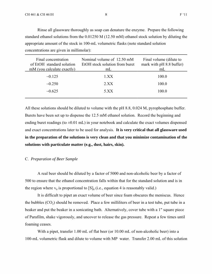
Rinse all glassware thoroughly as soap can denature the enzyme. Prepare the followingstandard ethanol solutions from the 0.01250 M (12.50 mM) ethanol stock solution by diluting theappropriate amount of the stock in 100-mL volumetric flasks (note standard solutionconcentrations are given in millimolar):

Final concentration of EtOH standard solutionmM (you calculate exactly)

Nominal volume of 12.50 mMEtOH stock solution from buret

mL

Final volume (dilute tomark with pH 8.8 buffer)

mL

~0.125 1.XX 100.0

~0.250 2.XX 100.0

~0.625 5.XX 100.0

All these solutions should be diluted to volume with the pH 8.8, 0.024 M, pyrophosphate buffer.

Burets have been set up to dispense the 12.5 mM ethanol solution. Record the beginning and

ending buret readings (to ±0.01 mL) in your notebook and calculate the exact volumes dispensed

and exact concentrations later to be used for analysis. It is very critical that all glassware used

in the preparation of the solutions is very clean and that you minimize contamination of the

solutions with particulate matter (e.g., dust, hairs, skin).

C. Preparation of Beer Sample

A real beer should be diluted by a factor of 5000 and non-alcoholic beer by a factor of

500 to ensure that the ethanol concentration falls within that for the standard solution and is in

the region where v0 is proportional to [S]0 (i.e., equation 4 is reasonably valid.)

It is difficult to pipet an exact volume of beer since foam obscures the meniscus. Hence

the bubbles (CO2) should be removed. Place a few milliliters of beer in a test tube, put tube in a

beaker and put the beaker in a sonicating bath. Alternatively, cover tube with a 1" square piece

of Parafilm, shake vigorously, and uncover to release the gas pressure. Repeat a few times until

foaming ceases.

With a pipet, transfer 1.00 mL of flat beer (or 10.00 mL of non-alcoholic beer) into a

100-mL volumetric flask and dilute to volume with MP water. Transfer 2.00 mL of this solution

CH 461 & CH 461H F ‘119

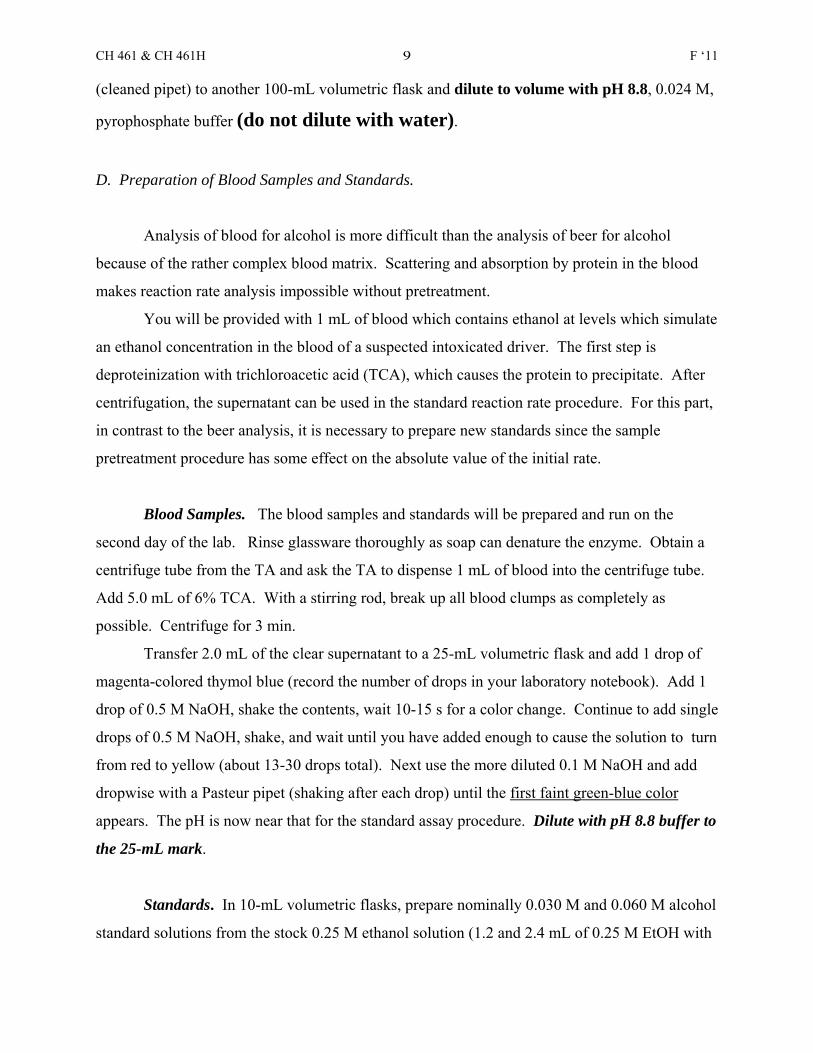
(cleaned pipet) to another 100-mL volumetric flask and dilute to volume with pH 8.8, 0.024 M,

pyrophosphate buffer (do not dilute with water).

D. Preparation of Blood Samples and Standards.

Analysis of blood for alcohol is more difficult than the analysis of beer for alcohol

because of the rather complex blood matrix. Scattering and absorption by protein in the blood

makes reaction rate analysis impossible without pretreatment.

You will be provided with 1 mL of blood which contains ethanol at levels which simulate

an ethanol concentration in the blood of a suspected intoxicated driver. The first step is

deproteinization with trichloroacetic acid (TCA), which causes the protein to precipitate. After

centrifugation, the supernatant can be used in the standard reaction rate procedure. For this part,

in contrast to the beer analysis, it is necessary to prepare new standards since the sample

pretreatment procedure has some effect on the absolute value of the initial rate.

Blood Samples. The blood samples and standards will be prepared and run on the

second day of the lab. Rinse glassware thoroughly as soap can denature the enzyme. Obtain a

centrifuge tube from the TA and ask the TA to dispense 1 mL of blood into the centrifuge tube.

Add 5.0 mL of 6% TCA. With a stirring rod, break up all blood clumps as completely as

possible. Centrifuge for 3 min.

Transfer 2.0 mL of the clear supernatant to a 25-mL volumetric flask and add 1 drop of

magenta-colored thymol blue (record the number of drops in your laboratory notebook). Add 1

drop of 0.5 M NaOH, shake the contents, wait 10-15 s for a color change. Continue to add single

drops of 0.5 M NaOH, shake, and wait until you have added enough to cause the solution to turn

from red to yellow (about 13-30 drops total). Next use the more diluted 0.1 M NaOH and add

dropwise with a Pasteur pipet (shaking after each drop) until the first faint green-blue color

appears. The pH is now near that for the standard assay procedure. Dilute with pH 8.8 buffer to

the 25-mL mark.

Standards. In 10-mL volumetric flasks, prepare nominally 0.030 M and 0.060 M alcohol

standard solutions from the stock 0.25 M ethanol solution (1.2 and 2.4 mL of 0.25 M EtOH with

CH 461 & CH 461H F ‘1110

the electronic pipet and dilute to 10 mL with the pH 8.8 buffer). Record the actual values you

dispensed and calculate the actual concentrations used later.

To make the ethanol standards appropriate for the analysis of blood (i.e., similar in

solution composition and pH to the blood samples), mix 1 mL of each EtOH standard with 5.0

mL of 6% TCA. Transfer 2.0 mL of this mixture to a 25-mL volumetric flask, add thymol blue,

adjust the pH, and bring up to volume with buffer. Note that after sample treatment, the

concentrations for the two standards are nominally 0.4 mM and 0.8 mM in ethanol in the

standard solutions (and nominally 0.32 mM and 0.64 mM in the solution in the cuvette).

E. Waste Disposal

Dilute ethanol solutions are nonhazardous and can be disposed down the drain. The

pellet from the centrifuge is nonhazardous and can be placed in solid waste (trash).

III. EXPERIMENTAL

A. Instrumentation

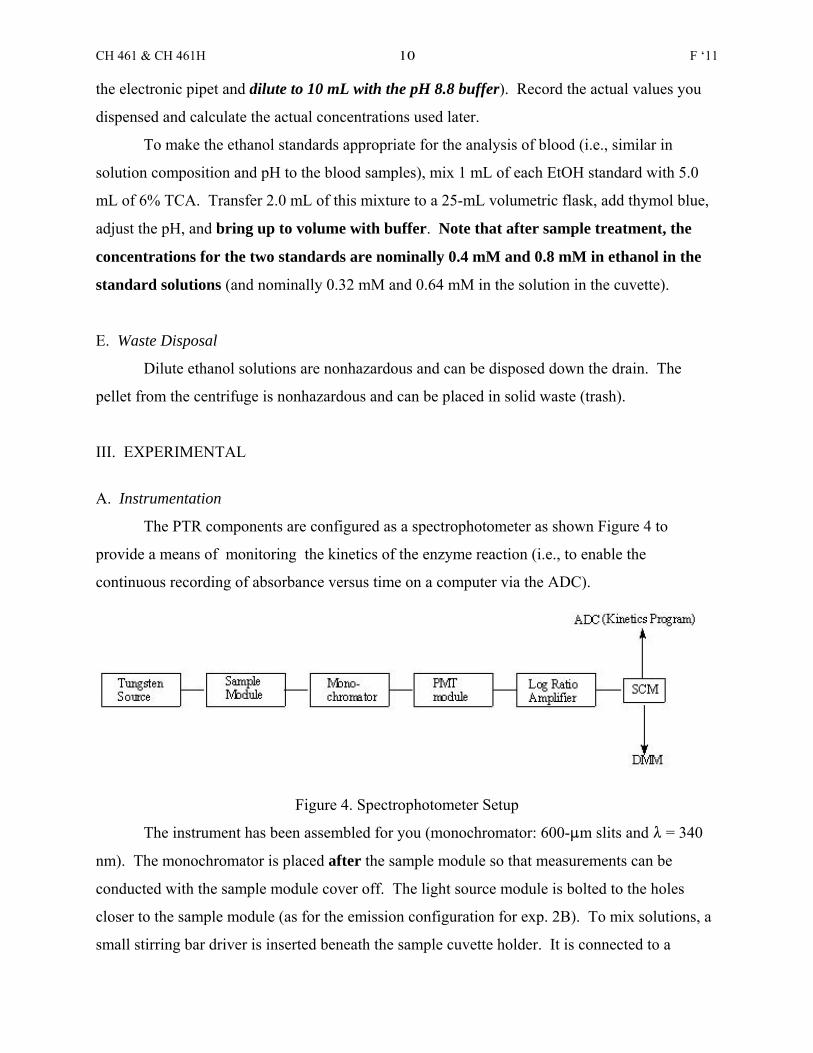
The PTR components are configured as a spectrophotometer as shown Figure 4 to

provide a means of monitoring the kinetics of the enzyme reaction (i.e., to enable the

continuous recording of absorbance versus time on a computer via the ADC).

Figure 4. Spectrophotometer Setup

The instrument has been assembled for you (monochromator: 600-:m slits and 8 = 340

nm). The monochromator is placed after the sample module so that measurements can be

conducted with the sample module cover off. The light source module is bolted to the holes

closer to the sample module (as for the emission configuration for exp. 2B). To mix solutions, a

small stirring bar driver is inserted beneath the sample cuvette holder. It is connected to a

CH 461 & CH 461H F ‘1111

controller to adjust the stirring speed. The use of linear absorbance monitoring is particularly

convenient for kinetics experiments. The electrical connections have been completed as

specified in the Appendix. You shouldn’t have to adjust anything, but you should verify the

PMT signal in Step 5 and the SCM signal in Step 6 before you begin.

B. Effect of Substrate Concentration and Analysis of Beer

In this part of the experiment, duplicate initial steady state rates v0 will be obtained for 7

different standard solutions of ethanol at concentrations from 0.125 - 250 mM. These results

will be used both for determination of vmax and Km and as calibration data for the determination

of ethanol in beer.

To obtain good data, it is critical that the operations and measurement conditions be

reproduced as closely as possible. Take extra care that the correct volumes are added and that the

timing of additions and stirring conditions are the same from run to run. Note that a provision for

temperature control of solutions and the sample cuvette holder would improve precision but is

not available at the PTR stations.

Initial Preparation

1. Prepare the three ethanol solutions indicated in section IIB and the one beer solution

(either alcohol containing or “alcohol free”) in section IIC.

2. Fill a clean wash bottle half full with the pH 8.8 buffer solution.

3. Obtain a small screw cap bottle of ADH and of NAD+ from the refrigerator and place

them in a beaker with ice near your instrument. Keep on ice at all times and keep the

caps on tight when not in use.

4. Confirm that a 250 :L automatic pipet, some pipet tips, and two sample cuvettes with

stirbars are at your station.

CH 461 & CH 461H F ‘1112

Measurement Procedure

1. Use a clean 2-mL volumetric pipet and pipet exactly 2.00 mL of the first standard

solution shown in Table I (p. 19) into each of the two sample cuvettes. Note that the test

solutions in the table are set up in duplicate runs for each ethanol concentration. Be sure

you rinse out the pipet with the next standard solution when switching to the next

concentration value (e.g., between runs 1B and 2A, etc.). Check that the pipet delivers all

2.00 mL.

2. Place a new tip on the automatic pipet and dispense 250 :L of NAD+ solution into each

of the cuvettes. When handling the pipet tips, do not touch the tips near the dispensing

end. Be absolutely sure you know how to properly use the automatic pipettor and

that the pipet tip is securely on. Ask if you have questions.

3. Insert a small magnetic stirring bar into the first cuvette, place the cuvette in the sample

holder, and adjust for an even stirring rate. Regular stirring is essential for the success of

this experiment. Note the orientation of the cuvette, mark the cuvette, and use the same

orientation throughout the experiment.

4. Set up the Kinetics program to record the data for this experiment. Choose the

computer delay time and measurement time specified in the ReadMe notes for Table I (p

18). Set the gain on the SCM to the value listed in Table I for the particular run and enter

that value in the Kinetics program. Be sure to save the output filename after the run and

use a new filename for each run. If you change the delay time, run the software before

adding samples to verify that the Kinetics program is indeed using the new delay time.

Adjust the gain on the PMT to make sure that the SCM output at the DMM is about +0.2

V at the start of each run.

CH 461 & CH 461H F ‘1113

5. Place a new tip on the automatic pipet, fill the automatic pipet with 250 :L of ADH

solution, check that the stirbar is spinning, and dispense the ADH solution into the

cuvette. At the time of injection, start the computer program and observe the reaction.

Allow the reaction to proceed at least 30 s. Measure and record the temperature of

run 1A in your lab notebook. Do not repeat the temperature measurement for the

other runs.

6. Using vacuum aspiration, remove the contents of the sample cuvette and rinse twice with

pH 8.8 buffer, being careful not to remove the stirbar. Repeat steps 2 through 5 for run

1B (except for the T measurement). It is very critical that the sample cuvettes be

thoroughly rinsed with buffer between analyses so that no residual alcohol is left

from a previous run. Avoid touching the pipet tip with your fingers because

proteases on your skin can deactivate the enzyme.

7. Now repeat steps 1 to 6 for runs 2A and 2B in Table I and repeat this sequence through

run 8B today.

This is the normal stopping place for the first day.

CH 461 & CH 461H F ‘1114

C. Determination of Alcohol in Blood.

Run duplicate assays of the two treated blood standards and the TCA /NaOH-treated

blood sample using the same procedure as before. That is, add 250 :L of NAD to 2.00 mL of

sample or standard added to the cuvette and inject 250 :L of ADH to initiate the runs (through

runs 11A & B). Finally return the sample cuvettes with stir bars to a TA.

IV. LAB REPORT

Your lab report should include an abstract, responses to Items A-H below, data Table 1,

and your lab notebook copy pages. Also include any raw data that you need to submit as

described in Item B below.

A. Prepare Table A showing the exact volumes of the stock 12.5 mM ethanol solution added and

the exact ethanol concentrations of the three standards that you prepared and used. Use these

values in subsequent calculations for the rate. Check that the buret readings are entered on

your lab notebook pages.

B. Determine and tabulate the initial rate for all runs from the slope of the linear regression

equation reported by the Kinetics program, which is also reported in the saved .csv file for each

run. Present this information in a Table B with columns for run number and rate in AU/min

from the program.

Note that the raw data and the rates reported by the Kinetics program are adjusted according to

the SCM gain value set on the front of the SCM module that you entered in the program before

starting the run. If the gain value was not entered in the program correctly, the rates calculated

by the program will not be correct- discuss with an instructor if needed.

If the rates reported by the Kinetics program are not consistent for duplicate runs or are

not producing a linear region for the lowest standards, then construct plots manually from the

CH 461 & CH 461H F ‘1115

.csv files and examine the quality of your raw data to ensure that you have initial rates

(AU min-1) that you can use with confidence for the rest of the experiment. Creating the plots

and determining the slopes from the raw data is relatively quick and easy if you use the hints in

the Appendix.

If the data are not smooth and regular, you may have to edit the raw data to eliminate

clear outliers and to capture the true rate of the enzyme catalyzed reaction. Editing of raw data

should not be undertaken without serious thought; if you have questions, ask. If you do edit the

raw data, always keep a copy of the original data (see Appendix) and include in your report a

graph with the complete original data set, the data that you retained for calculation of the rate,

and your justification for eliminating the points that you did. Be sure the rate reflects the initial

stage of the reaction -- if the rate starts to plateau, don’t use the plateau, but determine the initial

(fastest) rate by drawing a tangent to the initial part of the absorbance vs. time curve where the

rate is linear in time (if working in Excel, set a second series for the initial rate points).

C. Prepare Table C. with the data that you will use for the rest of the report. Show a sample

calculation for each part. Table C should have 11 rows of data (7 rows for the ethanol standards,

1 for the beer sample, 2 for the blood standards and 1 for the blood sample) and 5 columns

labeled as follows:

col 1. Sample ID (e.g., std 0.125 mM, beer sample 1, etc.)

col 2. Exact concentration of EtOH standard (mM) in the cuvette. This value is [S]0.

Values should be calculated from dilution of the volume of EtOH standard delivered

from the buret and should be close to those in column 2 in Table 1. For the beer and

blood samples, just identify the sample in this column.

col 3. Average initial rate in )A/min, determine from the average of the rates of the duplicate

runs.

col 4. Average initial rate (v0) in :mol/mL/min (from equation 7 and the rate data in the

preceding column).

col 5. Values for v0 /[S]0.

CH 461 & CH 461H F ‘1116

D. Prepare a Plot D of v0 versus v0 /[S]0 from 2.5 to 80 mM, report the slope and intercept, and

determine the values of Km and vmax. Do not include data from beer or blood samples.

E. Make Plot E of initial rate (:mol/mL/min) versus substrate concentration (i.e., v0 vs. [S]0)

over the ethanol concentration range of 0.5 to 200 mM.

• Do the data suggest a pseudo-zero region referred to in the derivation of equation 3?

Explain.

• Estimate vmax and Km by manual extrapolation on the plot and label both of these on the

plot. Do not perform a regression fit to the data because the simple unweighted

regression does not work well.

• Compare the values vmax and Km with those from part D. Comment on the comparison.

F. From the value of vmax calculated above and the known concentration (mg/mL) of enzyme in

the cuvette, calculate the specific activity of the enzyme in units/mg. Check the course web page

for the exact concentration of the ADH stock solution in the small brown bottle you worked

with (note this is not the concentration in the cuvette !).

G. Make an expanded Plot G of initial rate versus known substrate concentration (i.e., v0 vs.

[S]0) over the standard substrate concentration range of 0 to 0.5 mM in the cuvette.

• Do the data clearly show the first order region referred to in the derivation of equation 4?

Mark the region on plot and explain what this means.

• Use the slope and intercept of this plot to estimate the molar concentration of alcohol in

the reaction mixture for the diluted beer sample.

• Calculate the molar EtOH concentration in the original beer.

• Calculate the % (w/v) as (g ethanol/100 mL) in the original bottle of beer.

CH 461 & CH 461H F ‘1117

H. Make a separate Plot H of initial rate versus substrate concentration (v0 vs. [S]0) for the

blood standards (use the final cuvette values) and assume the origin is one point in the

calibration. Comment on how these initial rates for blood standards compare with the initial

rates from the beer standards (runs 1 & 2 and 4). If they are different, briefly explain what might

make them different.

1. Use the slope and intercept from the plot of the blood standards and estimate the molar

alcohol concentration in the reaction mixture for the diluted blood sample. Calculate the

molar EtOH concentration in the original blood sample and the %(w/v) EtOH (i.e., g/100

mL) in the original blood sample.

2. In Oregon, an EtOH blood level of 0.08%(w/v) or greater is considered conclusive

presumption of intoxication. What does your blood analysis indicate about the chances

in court of the driver from whom the blood was supposedly taken?

3. How many 12 oz bottles of the beer of the type analyzed here would an average person

have to drink to bring his/her blood alcohol level up to the value you determined for the

blood sample? When calculating the number of bottles needed, consider that out of 40 L

of aqueous fluids in an average adult, 5 L are blood. The transfer of ethanol from the

blood to various body fluids is very rapid so that the concentration of ethanol in blood

and other aqueous bodily fluids is taken to be equal. Assume the number of calculated

bottles are consumed in a span of two minutes and that all the alcohol consumed passes

directly into the blood stream.

CH 461 & CH 461H F ‘1118

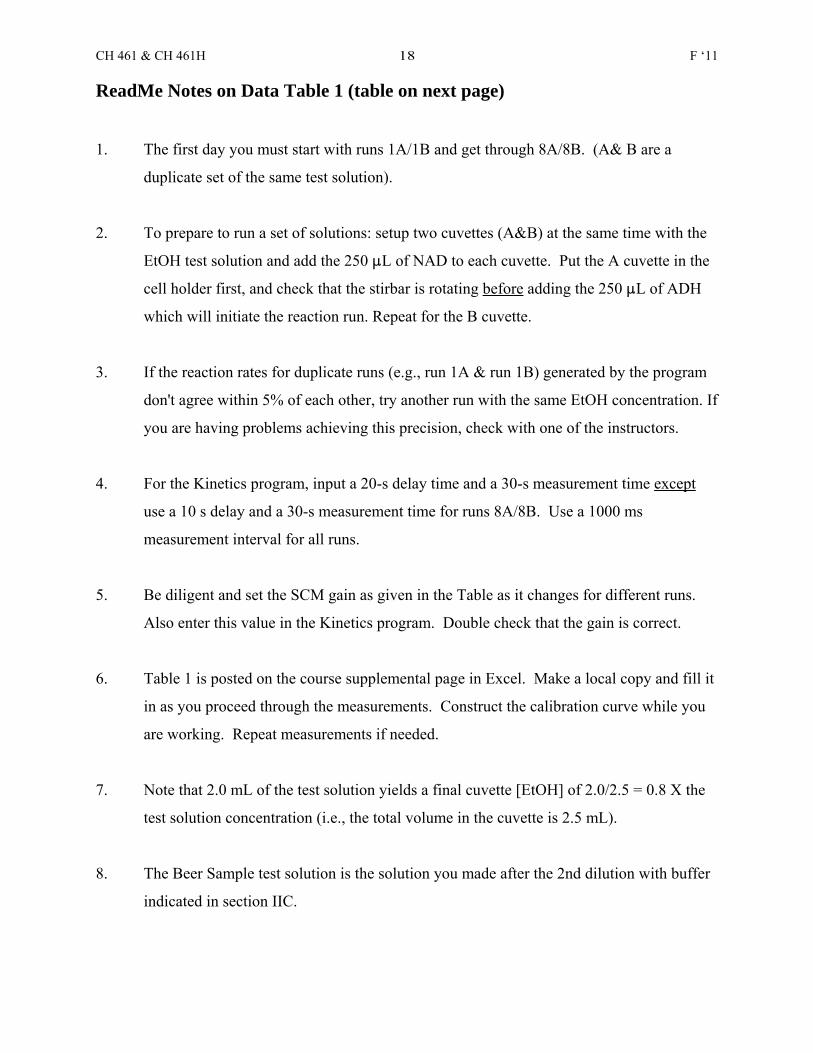
ReadMe Notes on Data Table 1 (table on next page)

1. The first day you must start with runs 1A/1B and get through 8A/8B. (A& B are a

duplicate set of the same test solution).

2. To prepare to run a set of solutions: setup two cuvettes (A&B) at the same time with the

EtOH test solution and add the 250 :L of NAD to each cuvette. Put the A cuvette in the

cell holder first, and check that the stirbar is rotating before adding the 250 :L of ADH

which will initiate the reaction run. Repeat for the B cuvette.

3. If the reaction rates for duplicate runs (e.g., run 1A & run 1B) generated by the program

don't agree within 5% of each other, try another run with the same EtOH concentration. If

you are having problems achieving this precision, check with one of the instructors.

4. For the Kinetics program, input a 20-s delay time and a 30-s measurement time except

use a 10 s delay and a 30-s measurement time for runs 8A/8B. Use a 1000 ms

measurement interval for all runs.

5. Be diligent and set the SCM gain as given in the Table as it changes for different runs.

Also enter this value in the Kinetics program. Double check that the gain is correct.

6. Table 1 is posted on the course supplemental page in Excel. Make a local copy and fill it

in as you proceed through the measurements. Construct the calibration curve while you

are working. Repeat measurements if needed.

7. Note that 2.0 mL of the test solution yields a final cuvette [EtOH] of 2.0/2.5 = 0.8 X the

test solution concentration (i.e., the total volume in the cuvette is 2.5 mL).

8. The Beer Sample test solution is the solution you made after the 2nd dilution with buffer

indicated in section IIC.

CH 461 & CH 461H F ‘1119

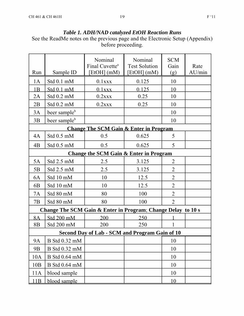
Table 1. ADH/NAD catalyzed EtOH Reaction RunsSee the ReadMe notes on the previous page and the Electronic Setup (Appendix)

before proceeding.

Run Sample ID

NominalFinal Cuvettea [EtOH] (mM)

NominalTest Solution[EtOH] (mM)

SCMGain(g)

Rate AU/min

1A Std 0.1 mM 0.1xxx 0.125 101B Std 0.1 mM 0.1xxx 0.125 102A Std 0.2 mM 0.2xxx 0.25 102B Std 0.2 mM 0.2xxx 0.25 103A beer sampleb 103B beer sampleb 10

Change The SCM Gain & Enter in Program4A Std 0.5 mM 0.5 0.625 5

4B Std 0.5 mM 0.5 0.625 5Change the SCM Gain & Enter in Program

5A Std 2.5 mM 2.5 3.125 25B Std 2.5 mM 2.5 3.125 26A Std 10 mM 10 12.5 26B Std 10 mM 10 12.5 27A Std 80 mM 80 100 27B Std 80 mM 80 100 2

Change The SCM Gain & Enter in Program; Change Delay to 10 s8A Std 200 mM 200 250 18B Std 200 mM 200 250 1

Second Day of Lab - SCM and Program Gain of 109A B Std 0.32 mM 109B B Std 0.32 mM 10

10A B Std 0.64 mM 1010B B Std 0.64 mM 1011A blood sample 1011B blood sample 10

CH 461 & CH 461H F ‘1120

V. References

Enzyme kinetics are discussed in the following books:

a. F. J. Reithel, "Concepts in Biochemistry", pp. 6-10, New York, McGraw-Hill Book Co.,

1967

b. A. White, P. Handler, and E. L. Smith, "Principles of Biochemistry", Fourth Ed., pp. 223-

246, New York, McGraw-Hill Book Co., 1968.

c. H. R. Mahler and E. H. Cordes, "Biological Chemistry", New York, Harper and Row,

1966.

d. M. Dixon and E. C. Webb, "Enzymes", Academic Press Inc., New York, 1958.

e. A. L. Lehninger, "Biochemistry", Worth Publishers, Inc., New York, 1970.

f. W. P. Jencks, "Catalysis in Chemistry and Enzymology", McGraw-Hill, New York,

1969.

g. J. Westley, "Enzymatic Catalysis", Harper and Row, New York, 1969.

h. M. L. Bender and L. J. Brubacher, "Catalysis and Enzyme Action", McGraw-Hill, New

York, 1973.

I. G. C. Guilbault, "Enzymatic Methods of Analysis", Pergamon Press, Oxford, 1970.

Pyridine nucleotide coenzymes are discussed in:

j. T. P. Singer and E. B. Kearney, Advanc. Enzymol., 15, 79 (1954).

Yeast alcohol dehydrogenase is reviewed by:

k. H. Snud and H. Theorell, "Alcohol Dehydrogenases", in The Enzymes, Vol. 7, 2nd Ed.,

P. D. Boyer, H. Lardy, and K. Myrback, eds., p. 25, Academic Press, Inc., New York,

1963.

The evolution of ethanol from the body is discussed in:

l. G. V. Calder, J. Chem. Ed., 51, 19 (1974).

CH 461 & CH 461H F ‘1121

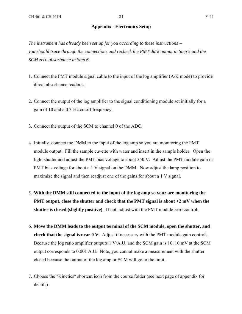
Appendix - Electronics Setup

The instrument has already been set up for you according to these instructions --

you should trace through the connections and recheck the PMT dark output in Step 5 and the

SCM zero absorbance in Step 6.

1. Connect the PMT module signal cable to the input of the log amplifier (A/K mode) to provide

direct absorbance readout.

2. Connect the output of the log amplifier to the signal conditioning module set initially for a

gain of 10 and a 0.3-Hz cutoff frequency.

3. Connect the output of the SCM to channel 0 of the ADC.

4. Initially, connect the DMM to the input of the log amp so you are monitoring the PMT

module output. Fill the sample cuvette with water and insert in the sample holder. Open the

light shutter and adjust the PMT bias voltage to about 350 V. Adjust the PMT module gain or

PMT bias voltage for about a 1 V signal on the DMM. Now adjust the lamp position to

maximize the signal and then readjust one of the gains for about a 1 V signal.

5. With the DMM still connected to the input of the log amp so your are monitoring the

PMT output, close the shutter and check that the PMT signal is about +2 mV when the

shutter is closed (slightly positive). If not, adjust with the PMT module zero control.

6. Move the DMM leads to the output terminal of the SCM module, open the shutter, and

check that the signal is near 0 V. Adjust if necessary with the PMT module gain controls.

Because the log ratio amplifier outputs 1 V/A.U. and the SCM gain is 10, 10 mV at the SCM

output corresponds to 0.001 A.U. Note, you cannot make a measurement with the shutter

closed because the output of the log amp or SCM will go to the limit.

7. Choose the "Kinetics" shortcut icon from the course folder (see next page of appendix for

details).

CH 461 & CH 461H F ‘1122

Computer Program - Kinetics

The Kinetics computer program for calculating the rate is based on the data acquisition

program you have used throughout the term. The user inputs a delay, measurement time, and the

SCM gain. When the user signals to start the measurement cycle (ENTER), the computer times

the delay chosen so that the reagents can mix and the reaction rate can reach full velocity. After

the delay time, the computer takes and stores a voltage reading every second for the

measurement time chosen. Next the program runs a linear regression and reports the slope and

intercept. You should then save the results of the regression and the raw data to a .csv file.

Each student in the group should have access to the full set of .csv files. Check the units for time

and make sure that you are using minutes in the calculations.

Creating Plots from Similar Sets of Data in Excel

Graphing Multiple runs using a template in Excel: Constructing these plots is relatively

quick and easy if you take the first data set (Run 1A), make the graph, add title, labels, etc. and a

trend line with slope and intercept displayed.

Method 1: Then save this spreadsheet as Run01A.xls and then save it again as Run01B.xls.

Then open the data for Run 1B, copy columns A and B, paste them into columns A & B of

Run01B.xls and save as Run01B.xls. Et cetera. This way you don't have to waste any time

reconfiguring the graphs.

Method 2: Alternative method to copy: right click on the tab name at the bottom and select

“move or copy” then check the box for “create a copy”. Once copied, right click on the new

spreadsheet page tab and rename it to Run01B, and proceed as above.