Existence results for some elliptic equations involving ... YANE.pdf · Ao amigo Nacib e a minha prima Sara pela disponibilidade e cuidado em me ajudar nas correções com o inglês

Universidade Federal da Paraíba

Universidade Federal de Campina Grande

Programa Associado de Pós-Graduação em Matemática

Doutorado em Matemática

Existence results for some ellipticequations involving the fractional

Laplacian operator and critical growth

por

Yane Lísley Ramos Araújo

João Pessoa - PB

Dezembro/2015

Existence results for some ellipticequations involving the fractional

Laplacian operator and critical growth

por

Yane Lísley Ramos Araújo †

sob orientação do

Prof. Dr. Manassés Xavier de Souza

Tese apresentada ao Corpo Docente do Programa

Associado de Pós-Graduação em Matemática -

UFPB/UFCG, como requisito parcial para obtenção do

título de Doutor em Matemática.

João Pessoa - PB

Dezembro/2015

†Este trabalho contou com apoio nanceiro da Capes.

ii

A663e Araújo, Yane Lísley Ramos. Existence results for some elliptic equations involving the

fractional Laplacian operator and critical growth / Yane Lísley Ramos Araújo.- João Pessoa, 2015.

111f. Orientador: Manassés Xavier de Souza Tese (Doutorado) - UFPB-UFCG 1. Matemática. 2. Laplaciano fracionário. 3. Métodos

variacionais. 4. Desigualdade de Trudinger-Moser. 5. Expoente crítico de Sobolev.

UFPB/BC CDU: 51(043)

Resumo

Neste trabalho provamos alguns resultados de existência e multiplicidade de soluções

para equações do tipo

(−∆)αu+ V (x)u = f(x, u) em RN ,

onde 0 < α < 1, N ≥ 2α, (−∆)α denota o Laplaciano fracionário, V : RN → R é uma

função contínua que satisfaz adequadas condições e f : RN×R→ R é uma função con-

tínua que pode ter crescimento crítico no sentido da desigualdade de Trudinger-Moser

ou no sentido do expoente crítico de Sobolev. A m de obter nossos resultados usa-

mos métodos variacionais combinados com uma versão do Princípio de Concentração-

Compacidade devido à Lions.

Palavras-chave: Laplaciano fracionário; métodos variacionais; desigualdade de Trudinger-

Moser; expoente crítico de Sobolev.

iv

Abstract

In this work we prove some results of existence and multiplicity of solutions for equa-

tions of the type

(−∆)αu+ V (x)u = f(x, u) in RN ,

where 0 < α < 1, N ≥ 2α, (−∆)α denotes the fractional Laplacian, V : RN → R is a

continuous function that satisfy suitable conditions and f : RN×R→ R is a continuous

function that may have critical growth in the sense of the Trudinger-Moser inequality

or in the sense of the critical Sobolev exponent. In order to obtain our results we

use variational methods combined with a version of the Concentration-Compactness

Principle due to Lions.

Keywords: Fractional Laplacian; variational methods; Trudinger-Moser's inequality;

critical Sobolev exponent.

v

Agradecimentos

A Deus pois só Ele é capaz de nos dar força para alcançarmos nossos objetivos.

Aos meus pais Ana Rita e Gildeval por todo amor, dedicação e apoio incondicional. Ao

meu irmão Tarles Walker e a minha madrinha Ana por sempre acreditarem em mim.

Ao meu esposo Reginaldo Junior pelo amor, companheirismo, compreensão e toda

ajuda indispensável à realização deste trabalho.

Ao Prof. Manassés Xavier de Souza por ter me concedido a oportunidade de estudar

com o mesmo, por toda orientação, dedicação e empenho na realização deste trabalho.

Ao meu amigo-irmão Gilson por ser um porto seguro para mim ao longo de toda a

jornada.

Ao amigo Nacib e a minha prima Sara pela disponibilidade e cuidado em me ajudar

nas correções com o inglês.

Aos meus professores Éder Mateus de Souza, João de Azevedo Cardeal e Fabíola de

Oliveira Pedreira Lima por serem inspirações para mim desde o ensino médio e a gra-

duação. Aos professores de Pós-Graduação do DM por todos os ensinamentos trans-

mitidos, em especial aos professores Everaldo Souto de Medeiros e Uberlandio Batista

Severo.

A minha irmã de coração Pammella e aos demais colegas do DM/UFPB que por muitas

vezes foram minha família dando apoio e diminuindo o fardo que é está longe de casa,

em especial a Diego, Rodrigo, Ricardo Burity, Gustavo, Valdecir, Diana, Daniel.

Aos membros da banca pelas valiosas contribuições para a versão nal deste trabalho.

A todos que direta ou indiretamente contribuíram para a conlusão deste trabalho.

À Capes pelo apoio nanceiro.

vi

Dedicatória

À minha família.

vii

Contents

Introduction . . . . . . . . . . . . . . . . . . . . . . . . . . . . . . . . . . . 1

Notation and terminology . . . . . . . . . . . . . . . . . . . . . . . . . . 11

1 Semilinear elliptic equations for the fractional Laplacian operator in-

volving critical exponential growth 13

Motivation and main results . . . . . . . . . . . . . . . . . . . . . . . . . . . 13

Some preliminary results . . . . . . . . . . . . . . . . . . . . . . . . . . . . . 19

The variational framework . . . . . . . . . . . . . . . . . . . . . . . . . . . . 23

Palais-Smale compactness condition . . . . . . . . . . . . . . . . . . . . . . . 26

Estimate of the minimax level . . . . . . . . . . . . . . . . . . . . . . . . . . 32

Proofs of Theorem 1.1 and 1.2 . . . . . . . . . . . . . . . . . . . . . . . . . . 33

2 On nonlinear perturbations of a periodic fractional Schrödinger equa-

tion with critical exponential growth 34


A periodic problem . . . . . . . . . . . . . . . . . . . . . . . . . . . . . 35

An asymptotically periodic problem . . . . . . . . . . . . . . . . . . . . 37

Some preliminary results . . . . . . . . . . . . . . . . . . . . . . . . . . . . . 39

The functional setting . . . . . . . . . . . . . . . . . . . . . . . . . . . 39

Trudinger-Moser type inequalities . . . . . . . . . . . . . . . . . . . . . 41

A Concentration-Compactness Principle . . . . . . . . . . . . . . . . . 43

Existence of a solution for the periodic problem . . . . . . . . . . . . . . . . 45

Minimax level . . . . . . . . . . . . . . . . . . . . . . . . . . . . . . . . 47

On Palais-Smale sequences . . . . . . . . . . . . . . . . . . . . . . . . . 47

viii

Proof of Theorem 2.1 . . . . . . . . . . . . . . . . . . . . . . . . . . . . 49

Existence of a solution for the asymptotically periodic problem . . . . . . . . 50

Proof of Theorem 2.2 . . . . . . . . . . . . . . . . . . . . . . . . . . . . 51

3 A class of asymptotically periodic fractional Schrödinger equations

with Sobolev critical growth 54


Notations, denitions and variational setting . . . . . . . . . . . . . . . . . . 58

Preliminary results . . . . . . . . . . . . . . . . . . . . . . . . . . . . . . . . 61

Versions of the Mountain Pass Theorem . . . . . . . . . . . . . . . . . 61

Mountain pass geometry . . . . . . . . . . . . . . . . . . . . . . . . . . 62

Behaviour of the Cerami sequences . . . . . . . . . . . . . . . . . . . . 63

Estimate of the minimax level . . . . . . . . . . . . . . . . . . . . . . . . . . 68

Test functions . . . . . . . . . . . . . . . . . . . . . . . . . . . . . . . . 68

Convergence results . . . . . . . . . . . . . . . . . . . . . . . . . . . . . . . . 73

Proof of Theorem 3.1 . . . . . . . . . . . . . . . . . . . . . . . . . . . . . . . 77

Proof of Theorem 3.2 . . . . . . . . . . . . . . . . . . . . . . . . . . . . . . . 83

Appendix

A Auxiliary results 85

Fractional Sobolev spaces and the fractional Laplacian operator . . . . . . . 85

Variational formulation . . . . . . . . . . . . . . . . . . . . . . . . . . . . . . 87

Dierentiability of the functional I . . . . . . . . . . . . . . . . . . . . . . . 89

A example without the (AR) condition . . . . . . . . . . . . . . . . . . . . . 94

References 99

ix

Introduction

In this work, we study the existence and multiplicity of solutions for elliptic

equations of the type

(−∆)αu+ V (x)u = f(x, u) in RN , (0.1)

where 0 < α < 1, N ≥ 2α, V : RN → R and f : RN ×R→ R are continuous functions

that satisfy suitable conditions and (−∆)α denotes the fractional Laplacian which can

be dened for a suciently regular function u : R→ R by

(−∆)αu(x) = −1

2C(N,α)

∫RN

u(x+ y) + u(x− y)− 2u(x)

|y|N+2αdy, ∀x ∈ RN .

For details about this operator see Appendix A.

Part of the interest on those equations arises in the search of standing waves

solutions for the fractional Schrödinger equation

i∂ψ

∂t= (−∆)αψ + (V (x) + ω)ψ − f(x, ψ), (x, t) ∈ RN × R, (0.2)

where ω ∈ R, V : RN → R is an external potential function, f : RN × R → R is a

continuous function and 0 < α < 1 is a xed parameter. Standing waves solutions to

Equation (0.2) are solutions of the form

ψ(x, t) = u(x) exp(−iωt),

where u solves elliptic Equation (0.1).

Equation (0.2) comes from an expansion of the Feynman path integral from

Brownian-like to Lévy-like quantum mechanical paths (see [31] and [32]). It is known,

but not completely trivial, that (−∆)α reduces to the standard Laplacian−∆ if α→ 1−

1

(see [17]). Thus, when α = 1, the Lévy dynamics becomes the Brownian dynamics,

and Equation (0.2) reduces to the classical Schrödinger equation

i∂ψ

∂t= −∆ψ + (V (x) + ω)ψ − f(x, ψ), (x, t) ∈ RN × R.

Motivated by Equation (0.2), several studies have been performed for elliptic

equations involving the fractional Laplacian operator. In the sequel, we will list some

papers related with the existence of solutions to Equation (0.1) that may be found in

the literature.

Let us begin with the progress involving subcritical nonlinearities. Using the

Nehari variational principle, in [11], Cheng proved the existence of a nontrivial solution

of the fractional Schrödinger equation

(−∆)αu+ V (x)u = |u|q−2u, x ∈ RN , (0.3)

with 2 < q < 2∗α if N > 2α or 2 < q < ∞ if N ≤ 2α, where 2∗α := 2N/(N − 2α)

is the critical Sobolev exponent. Ground states are found by imposing a coercivity

assumption on V (x),

lim|x|→+∞

V (x) = +∞. (0.4)

In [41], Secchi proved the existence of a nontrivial solution under less restrictive

assumptions on f(x, u). He obtained the existence of a ground state by the method

used in [24]. It is worthwhile to notice that in [11] and [41] the hypothesis (0.4) is

assumed on V (x) in order to overcome the problem of lack of compactness, typical of

elliptic problems dened in unbounded domains. In [18], Dipierro et al. considered the

existence of radially symmetric solutions of (0.3) in the situation where V (x) does not

depend explicitly on the space variable x. For the rst time, using rearrangement tools

and following the ideas of Berestycki and Lions [5], the authors proved the existence of

a nontrivial, radially symmetric solution to

(−∆)αu+ u = |u|q−2u, x ∈ RN ,

where 2 < q < 2∗α if N > 2α or 2 < q <∞ if N ≤ 2α.

After the pioneering works by Brezis and Nirenberg in [8], elliptic problems with

critical growth have had many progresses in several directions. For the fractional

2

Laplacian, we would like to mention [21, 28, 43] and the references therein. More

specically, Shang et al. in [43] considered the existence of solutions for the problem

(−∆)αu+ V (x)u = |u|2∗α−2u+ λ|u|q−2u, x ∈ RN ,

where λ > 0 is a parameter, 2 < q < 2∗α and N > 2α. The potential V : RN → R is

a continuous function satisfying 0 < infx∈RN V (x) = V 0 < lim inf |x|→+∞ V (x) = V∞,

where V∞ <∞. This kind of hypothesis was rst introduced by Rabinowitz in [40].

J. M. do Ó et al. in [21] proved the existence of a solution of the fractional

Schrödinger equation

(−∆)αu+ V (x)u = |u|2∗α−2u+K(x)f(u), x ∈ RN ,

where V , K are continuous, V,K > 0 in RN with V (x)→ 0, K(x)→ 0, as |x| → +∞,

and f(u) behaves like |u|q−2u at innity, for some 2 < q < 2∗α and N > 2α. Moreover,

f(u) satises the so-called AmbrosettiRabinowitz condition, namely,

(AR) there existsµ ∈ (2, 2∗α) with 0 < µF (s) ≤ sf(s) for all s 6= 0, F (s) =

s∫0

f(t)dt.

With respect to the growth of the nonlinearity in problems of the type (0.1) in

the limiting case N = 2α, for N = 1 and α = 1/2, there exists a special situation

motivated by the Trudinger-Moser inequality. Precisely, it is known that the embed-

ding H1/2(R) → Lq(R) is continuous for any q ∈ [2,+∞), but H1/2(R) is not conti-

nuously embedded in L∞(R). However, T. Ozawa [39] and H. Kozono, T. Sato and H.

Wadade [29] proved a version of the Trudinger-Moser inequality. More precisely, they

proved that there exist positive constants ω and C such that, for all u ∈ H1/2(R) with

‖(−∆)1/4u‖2 ≤ 1, ∫R

(eβu2 − 1) dx ≤ C‖u‖2

2, for all β ∈ (0, ω]. (0.5)

Consequently, the maximal growth which allows us to treat (0.1) variationally in

H1/2(R) is of the type exponential.

Inequality (0.5) plays a crucial role in the study of problems that involved non-

linearities with exponential growth. For works involving this type of nonlinearities, we

3

would like to mention two papers, [23] and [25]. J. M. do Ó et al. in [23] proved the

existence of a solution for the fractional Schrödinger equation

(−∆)1/2u+ u = K(x)g(u),

where K is a positive function which can vanish at innity and g has exponential

growth. Iannizzotto and Squassina, in [25], considered the existence of solutions for

the problem (−∆)1/2u = f(u) in (0, 1),

u = 0 in R \ (0, 1),

where the nonlinearity has exponential growth.

Motivated by these studies and taking into consideration the behavior of the

potential V (x) and the types of nonlinearity f(x, s), in this work we obtain some

results of existence and multiplicity of solutions to Equation (0.1). Precisely:

In Chapter 1, we treat the limiting case N = 1, α = 1/2, more specically, we

study the equation

(−∆)1/2u+ V (x)u = f(x, u) + h in R, (0.6)

where (−∆)1/2 is dened in the Section 1, V : R → R is a continuous potential, h

belongs to the dual of an appropriate functional space, see Section 1, and f : R×R→ R

is a continuous function that has critical exponential growth, that is, there exists β0 > 0

such that

lim|s|→+∞

f(x, s)e−β|s|2

=

0, for all β > β0,

+∞, for all β < β0,

uniformly in x ∈ R.

We consider the following hypotheses under V (x):

(V1) there exists a positive constant B such that V (x) ≥ −B, for all x ∈ R;

(V2) the inmum

λ1 := infu∈X‖u‖2=1

1

2π

∫R2

(u(x)− u(y))2

|x− y|2dx dy +

∫R

V (x)u2 dx

is positive;

4

(V3) limR→∞

ν(R \BR) = +∞, where

ν(G) =

inf

u∈X0(G)‖u‖2=1

1

2π

∫R2

(u(x)− u(y))2

|x− y|2dx dy +

∫G

V (x)u2 dx if G 6= ∅;

∞ if G = ∅.

Here G is an open set in R and X0(G) = u ∈ X : u = 0 in R \G, where X

is dened in (1.3).

It is important to observe that the assumptions (V1) − (V3) allow that the potentials

may change sign.

In order to use a variational approach, we consider the following assumptions

about f(x, s):

(f1) 0 ≤ lims→0

f(x, s)

s< λ1, uniformly in x;

(f2) f is locally bounded in s, that is, for any bounded interval J ⊂ R, there exists

C > 0 such that |f(x, s)| ≤ C, for every (x, s) ∈ R× J ;

(f3) there exists θ > 2 such that

0 < θF (x, s) := θ

s∫0

f(x, t) dt ≤ sf(x, s), for all (x, s) ∈ R× R \ 0;

(f4) there exist constants s0,M0 > 0 such that

0 < F (x, s) ≤M0|f(x, s)|, for all |s| ≥ s0 and x ∈ R;

(f5) there exist constants p > 2 and Cp such that, for all s ≥ 0 and x ∈ R,

f(x, s) ≥ Cpsp−1,

with Cp >

[α0(p− 2)

2πκωp

](p−2)/2

Spp , where

Sp := infu∈X‖u‖p=1

1

2π

∫R2

(u(x)− u(y))2

|x− y|2dx dy +

∫R

V (x)u2 dx

1/2

,

and κ is given in (1.7).

With this we obtain the main results of this chapter:

5

Theorem 0.1. Suppose that (V1)− (V3) and (f1)− (f5) hold. Then there exists δ1 > 0

such that for each 0 < ‖h‖∗ < δ1, problem (0.6) has at least two weak solutions. One

of them with positive energy, and the other one with negative energy.

Theorem 0.2. Suppose that (V1) − (V3) and (f1) − (f5) hold. If h ≡ 0 (i.e., there is

no perturbation in (0.6)) then problem (0.6) has a weak solution with positive energy.

In order to prove Theorems 0.1 and 0.2, we need to check some conditions con-

cerning the mountain pass geometry and the compactness of the associated functional.

More specically, we show that the functional associated with the problem satises

the Palais-Smale condition. Then we use minimization to nd the rst solution with

negative energy and the Mountain Pass Theorem to obtain the existence of the second

solution with positive energy. The main diculties lie in the nonlocal operator involved

and in the critical exponential growth of the nonlinearity.

Our results complement the work in [25] since we considered that the domain

is all R. It also complement [11, 23, 41, 42], once we work with nonlinearities more

general than those treated by them and potentials that may change sign, vanish and

be unbounded.

In Chapter 2, we deal with the problem of existence of weak solutions to a class

of equations similar to those that we studied in Chapter 1, where V is a bounded

potential that belongs to a dierent class of those treated therein. We study two class

of problems:

The rst one (a periodic problem) is the following, (−∆)1/2u+ V0(x)u = f0(x, u) in R,

u ∈ H1/2(R) and u ≥ 0.(P0)

We consider that the function V0 : R → (0,+∞) is a continuous 1−periodic

function and f0 : R × R → R is a continuous 1−periodic function in x, which has

critical exponential growth in u. Since we are interested in the existence of nonnegative

solutions, we set f0(x, s) = 0 for all (x, s) ∈ R × (−∞, 0]. We also assume that the

nonlinearity f0(x, u) satises the conditions

(f0,1) lims→0

f0(x, s)

s= 0 uniformly in x ∈ R;

6

(f0,2) there exists a constant θ > 2 such that

0 < θF0(x, s) := θ

s∫0

f0(x, t) dt ≤ sf0(x, s), for all (x, s) ∈ R× (0,+∞);

(f0,3) for each xed x ∈ R, the function f0(x, s)/s is increasing with respect to s ∈ R;

(f0,4) there are constants p > 2 and Cp > 0 such that

f0(x, s) ≥ Cpsp−1, for all (x, s) ∈ R× [0,+∞),

where

Cp >

[(p− 2)θα0

(θ − 2)pω

](p−2)/2

Spp

and

Sp := infu∈H1/2(R)‖u‖p=1

1

2π

∫R2

|u(x)− u(y)|2

|x− y|2dxdy + ‖V ‖∞

∫R

u2 dx

1/2

.

Under these assumptions we have the rst result of Chapter 2:

Theorem 0.3. Assume that (f0,1)−(f0,4) hold. Then (P0) has a nonnegative nontrivial

weak solution.

The second problem (asymptotically periodic) that we study in this chapter is (−∆)1/2u+ V (x)u = f(x, u) in R,

u ∈ H1/2(R) and u ≥ 0,(P )

on which we consider the following conditions on the function V (x):

(V1) V : R→ [0,+∞) is a continuous function satisfying the conditions: V (x) ≤ V0(x)

for any x ∈ R and V0(x)− V (x)→ 0 as |x| → ∞;

We assume that the nonlinearity f : R × R → R is a continuous function that

has critical exponential growth in s, f(x, s) = 0 for all (x, s) ∈ R × (−∞, 0] and also

satises:

(f1) f(x, s) ≥ f0(x, s) for all (x, s) ∈ R× [0,+∞), and for all ε > 0, there exists η > 0

such that for s ≥ 0 and |x| ≥ η,

|f(x, s)− f0(x, s)| ≤ εeα0s2 ;

7

(f2) lims→0

f(x, s)


(f3) there exists a constant µ > 2 such that

0 < µF (x, s) := µ

s∫0

f(x, t) dt ≤ sf0(x, s), for all (x, s) ∈ R× (0,+∞);

(f4) for each xed x ∈ R, the function f(x, s)/s is increasing with respect to s ∈ R;

(f5) at least one of the nonnegative continuous functions V0(x)− V (x) and f(x, s)−

f0(x, s) is positive on a set of positive measure.

The second result of Chapter 2 is the following:

Theorem 0.4. Assume that (V1) and (f1) − (f5) hold. Then (P ) has a nonnegative

nontrivial weak solution.

In order to prove our results, we show that the weak limit of an appropriate

sequence of Palais Smale is a weak solution of the problem and we use a version of the

Concentration-Compactness Priniple due to Lions to show that this limit is nontrivial.

We point out that our results complete the study presented in [22, 23], since

we work with a general class of functions which are asymptotic to a nonautonomous

periodic function at innity. It also complements [10, 11, 18, 41], once we consider the

limiting case for N = 1 and α = 1/2 when the nonlinearity has exponential growth in

the sense of the Trudinger-Moser inequality. Moreover, it also complements [14], the

study of Chapter 1, once we consider that the potential V (x) belongs to a dierent

class from those treated there.

In Chapter 3, our main goal is to establish, under an asymptotic periodicity

condition at innity, the existence of a weak solution for the critical problem

(−∆)αu+ V (x)u = |u|2∗α−2u+ g(x, u), x ∈ RN , (0.7)

where 0 < α < 1, N > 2α, V : RN → R and g : RN ×R→ R are continuous functions.

Considering F the class of functions h ∈ C(RN) ∩ L∞(RN) such that, for every

ε > 0, the set x ∈ RN : |h(x)| ≥ ε has nite Lebesgue measure, we assume that V

satises:

8

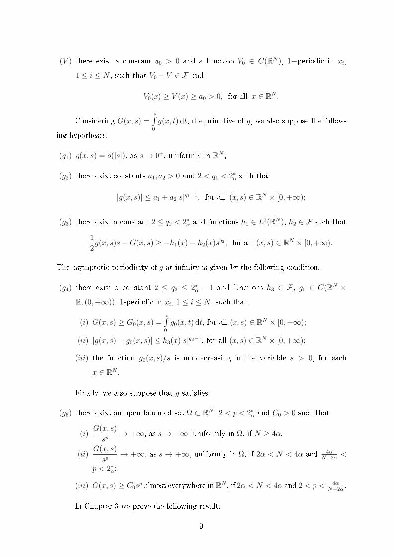
(V ) there exist a constant a0 > 0 and a function V0 ∈ C(RN), 1−periodic in xi,

1 ≤ i ≤ N , such that V0 − V ∈ F and

V0(x) ≥ V (x) ≥ a0 > 0, for all x ∈ RN .

Considering G(x, s) =s∫

0

g(x, t) dt, the primitive of g, we also suppose the follow-

ing hypotheses:

(g1) g(x, s) = o(|s|), as s→ 0+, uniformly in RN ;

(g2) there exist constants a1, a2 > 0 and 2 < q1 < 2∗α such that

|g(x, s)| ≤ a1 + a2|s|q1−1, for all (x, s) ∈ RN × [0,+∞);

(g3) there exist a constant 2 ≤ q2 < 2∗α and functions h1 ∈ L1(RN), h2 ∈ F such that

1

2g(x, s)s−G(x, s) ≥ −h1(x)− h2(x)sq2 , for all (x, s) ∈ RN × [0,+∞).

The asymptotic periodicity of g at innity is given by the following condition:

(g4) there exist a constant 2 ≤ q3 ≤ 2∗α − 1 and functions h3 ∈ F , g0 ∈ C(RN ×

R, (0,+∞)), 1-periodic in xi, 1 ≤ i ≤ N , such that:

(i) G(x, s) ≥ G0(x, s) =s∫

0

g0(x, t) dt, for all (x, s) ∈ RN × [0,+∞);

(ii) |g(x, s)− g0(x, s)| ≤ h3(x)|s|q3−1, for all (x, s) ∈ RN × [0,+∞);

(iii) the function g0(x, s)/s is nondecreasing in the variable s > 0, for each

x ∈ RN .

Finally, we also suppose that g satises:

(g5) there exist an open bounded set Ω ⊂ RN , 2 < p < 2∗α and C0 > 0 such that

(i)G(x, s)

sp→ +∞, as s→ +∞, uniformly in Ω, if N ≥ 4α;

(ii)G(x, s)

sp→ +∞, as s → +∞, uniformly in Ω, if 2α < N < 4α and 4α

N−2α<

p < 2∗α;

(iii) G(x, s) ≥ C0sp almost everywhere in RN , if 2α < N < 4α and 2 < p < 4α

N−2α.

In Chapter 3 we prove the following result.

9

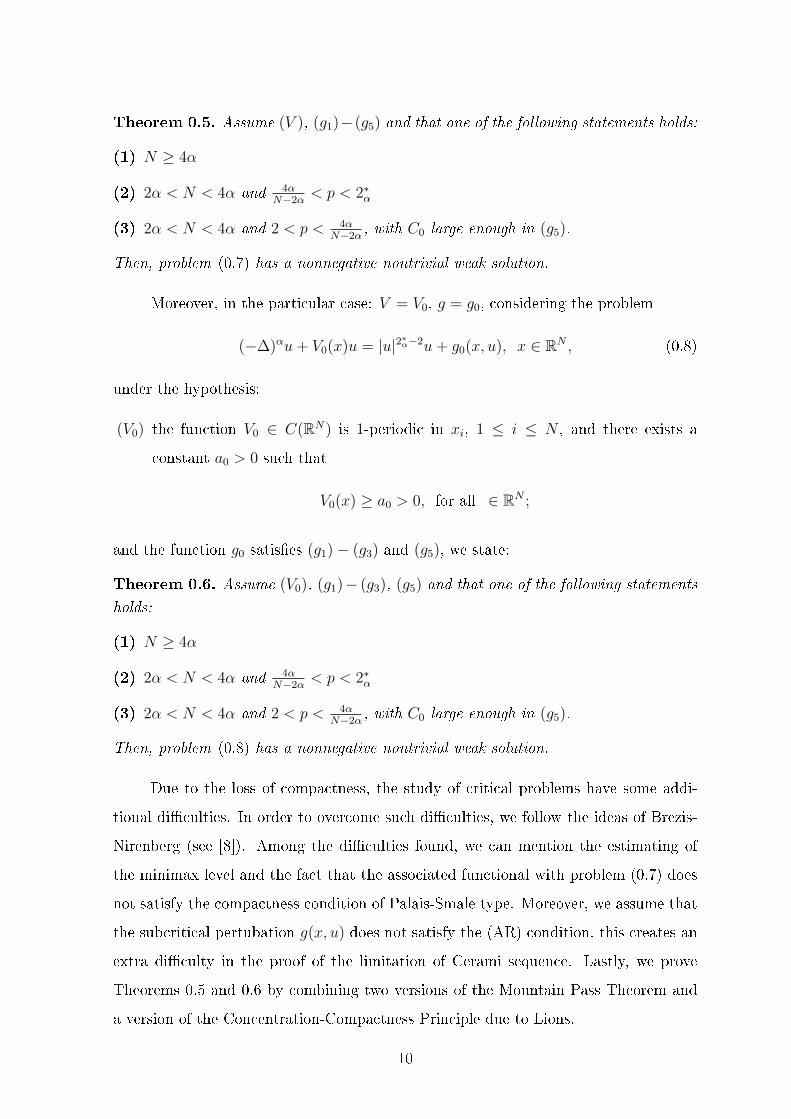
Theorem 0.5. Assume (V ), (g1)−(g5) and that one of the following statements holds:

(1) N ≥ 4α

(2) 2α < N < 4α and 4αN−2α

< p < 2∗α

(3) 2α < N < 4α and 2 < p < 4αN−2α

, with C0 large enough in (g5).

Then, problem (0.7) has a nonnegative nontrivial weak solution.

Moreover, in the particular case: V = V0, g = g0, considering the problem

(−∆)αu+ V0(x)u = |u|2∗α−2u+ g0(x, u), x ∈ RN , (0.8)

under the hypothesis:

(V0) the function V0 ∈ C(RN) is 1-periodic in xi, 1 ≤ i ≤ N , and there exists a

constant a0 > 0 such that

V0(x) ≥ a0 > 0, for all ∈ RN ;

and the function g0 satises (g1)− (g3) and (g5), we state:

Theorem 0.6. Assume (V0), (g1)− (g3), (g5) and that one of the following statements

holds:

(1) N ≥ 4α

(2) 2α < N < 4α and 4αN−2α

< p < 2∗α

(3) 2α < N < 4α and 2 < p < 4αN−2α

, with C0 large enough in (g5).


Due to the loss of compactness, the study of critical problems have some addi-

tional diculties. In order to overcome such diculties, we follow the ideas of Brezis-

Nirenberg (see [8]). Among the diculties found, we can mention the estimating of

the minimax level and the fact that the associated functional with problem (0.7) does

not satisfy the compactness condition of Palais-Smale type. Moreover, we assume that

the subcritical pertubation g(x, u) does not satisfy the (AR) condition, this creates an

extra diculty in the proof of the limitation of Cerami sequence. Lastly, we prove

Theorems 0.5 and 0.6 by combining two versions of the Mountain Pass Theorem and

a version of the Concentration-Compactness Principle due to Lions.

10

Our results complement the study made in [10,21,43] in the sense that the non-

linearity behaves like u2∗α−1 + g(x, u), where the subcritical perturbation g(x, u) does

not satisfy (AR) condition. Moreover, we also complement [10, 11, 18, 41] in the sense

that the potential V (x) belongs to a dierent class from those treated by them.

In order to do not get resorting to Introduction, and, for the sake of indepen-

dence of the chapters, we will present again, in each chapter, the main results and the

hypotheses about the functions V (x) and f(x, u).

11

Notation and terminology

In this work we will use the following symbology:

• C, C0, C1, C2, ... denote positive constants (possibly dierent);

• supp(f) denotes the support of the function f ;

• BR(x) denotes an open ball of radius R and center x; BR denotes an open ball

of radius R and center at origin and BR is the closed ball with center at origin

and radius R;

• BcR denotes the complement of BR;

• ,→ denote weak and strong convergence, respectively, in a normed space;

• u+ = maxu, 0 and u− = max−u, 0;

• XΩ denotes the characteristic function of the set Ω;

• ‖ · ‖1/2 denotes the norm in the space H1/2(R);

• ‖ · ‖∗ denotes the norm in the topologic dual space X∗;

• ‖ · ‖p denotes the standard Lp(RN)-norm;

• ‖ · ‖∞ denotes the standard L∞(RN)-norm;

12

Chapter 1

Semilinear elliptic equations for the

fractional Laplacian operator

involving critical exponential growth

This chapter is devoted to the paper [14], here we establish the existence and

multiplicity of weak solutions for a class of equations involving the fractional Laplacian

operator, potentials that may change sign and nonlinearities with critical exponential

growth. The proofs of our existence results rely on minimization methods and the

Mountain Pass Theorem.

Motivation and main results

The starting point of this chapter is to investigate the existence and multiplicity

of weak solutions for the following class of equations

(−∆)1/2u+ V (x)u = f(x, u) + h in R, (1.1)

where V : R → R is a continuous potential which may change sign, the nonlinearity

f(x, s) behaves like exp(α0s2) when |s| → +∞ for some α0 > 0, h belongs to the dual

of an appropriate functional space and (−∆)1/2 is the fractional Laplacian operator

which, for a suciently regular function u : R→ R, is dened by

(−∆)1/2u(x) = − 1

2π

∫R

u(x+ y) + u(x− y)− 2u(x)

|y|2dy. (1.2)

13

In order to study variationally (1.1), we consider a suitable subspace of the frac-

tional Sobolev space H1/2(R). Recall that H1/2(R) is dened as the space

H1/2(R) :=

u ∈ L2(R) :

|u(x)− u(y)||x− y|

∈ L2(R× R)

;

endowed with the norm

‖u‖1/2 :=

[u]21/2 +

∫R

|u|2 dx

1/2

,

where

[u]1/2 :=

∫R2

|u(x)− u(y)|2

|x− y|2dx dy

1/2

is the so-called Gagliardo semi-norm of u. For more details see Appendix (A).

Some suitable conditions on the potential V are assumed in order to apply a

variational framework considering the subspace of H1/2(R) given by

X =

u ∈ H1/2(R) :

∫R

V (x)u2 dx <∞

. (1.3)

More precisely, we suppose the following assumptions on V (x):

(V1) there exists a positive constant B such that V (x) ≥ −B, for all x ∈ R;

(V2) the inmum

λ1 := infu∈X‖u‖2=1

1

2π

∫R2

(u(x)− u(y))2

|x− y|2dx dy +

∫R

V (x)u2 dx

is positive;

(V3) limR→∞

ν(R \BR) = +∞, where

ν(G) =

inf

u∈X0(G)‖u‖2=1

1

2π

∫R2

(u(x)− u(y))2

|x− y|2dx dy +

∫G

V (x)u2 dx if G 6= ∅;

∞ if G = ∅.

Here G is an open set in R, X0(G) = u ∈ X : u = 0 in R \G.

14

The hypotheses (V1) and (V2) ensure that X is a Hilbert space when endowed

with the inner product

〈u, v〉 =1

2π

∫R2

(u(x)− u(y))(v(x)− v(y))

|x− y|2dx dy +

∫R

V (x)uv dx, u, v ∈ X,

which induces the norm ‖u‖ := 〈u, u〉1/2 (see Section 1).

In this context, we assume that h ∈ X∗ (dual space of X) and we say that u ∈ X

is a weak solution for (1.1) if for all v ∈ X,

1

2π

∫R2

(u(x)− u(y))(v(x)− v(y))

|x− y|2dx dy+

∫R

V (x)uv dx =

∫R

f(x, u)v dx+(h, v), (1.4)

where (·, ·) denotes the duality pairing between X and X∗.

We are interested in the case that the nonlinearity f(x, s) has the maximal growth

which allows us to study (1.1) by using a variational framework considering the space

X. More specically, we assume sucient conditions such that the weak solutions of

(1.1) become critical points of the Euler functional I : X → R dened by

I(u) =1

2‖u‖2 −

∫R

F (x, u) dx− (h, u),

where F (x, s) =

s∫0

f(x, t)dt.

In order to improve the presentation of the hypotheses on f(x, s), we recall some

well known facts involving the limiting Sobolev embedding Theorem in 1-dimension.

The Sobolev embedding assures that H1/2(R) → Lq(R) for any q ∈ [2,+∞); but

H1/2(R) is not continuously embedded in L∞(R) (for more details, see [17], [39]). In

this case the maximal growth of f(x, s), which allows us to study (1.1) by applying

a variational framework involving the space H1/2(R), is motivated by the Trudinger-

Moser inequality that was proved by H. Kozono, T. Sato and H. Wadade [29] and T.

Ozawa [39]. More precisely, they proved that there exist positive constants ω and C

such that for all u ∈ H1/2(R) with ‖(−∆)1/4u‖2 ≤ 1,∫R

(eαu2 − 1) dx ≤ C‖u‖2

2 , for all α ∈ (0, ω]. (1.5)

(See also some pioneering works such as [38], [45]).

15

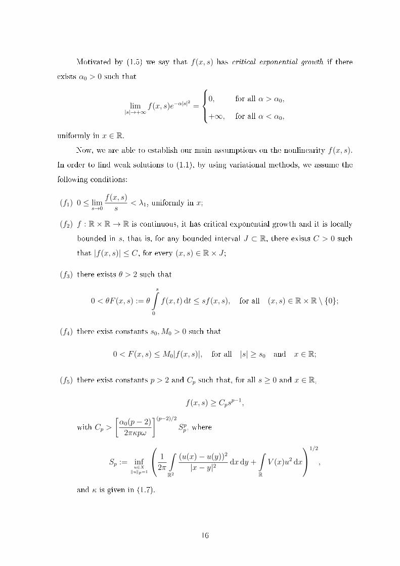
Motivated by (1.5) we say that f(x, s) has critical exponential growth if there

exists α0 > 0 such that

lim|s|→+∞

f(x, s)e−α|s|2

=

0, for all α > α0,

+∞, for all α < α0,


Now, we are able to establish our main assumptions on the nonlinearity f(x, s).

In order to nd weak solutions to (1.1), by using variational methods, we assume the

following conditions:

(f1) 0 ≤ lims→0

f(x, s)

s< λ1, uniformly in x;

(f2) f : R× R → R is continuous, it has critical exponential growth and it is locally

bounded in s, that is, for any bounded interval J ⊂ R, there exists C > 0 such

that |f(x, s)| ≤ C, for every (x, s) ∈ R× J ;

(f3) there exists θ > 2 such that

0 < θF (x, s) := θ

s∫0

f(x, t) dt ≤ sf(x, s), for all (x, s) ∈ R× R \ 0;

(f4) there exist constants s0,M0 > 0 such that

0 < F (x, s) ≤M0|f(x, s)|, for all |s| ≥ s0 and x ∈ R;

(f5) there exist constants p > 2 and Cp such that, for all s ≥ 0 and x ∈ R,

f(x, s) ≥ Cpsp−1,

with Cp >

[α0(p− 2)

2πκpω

](p−2)/2

Spp , where


1

2π

∫R2

(u(x)− u(y))2

|x− y|2dx dy +

∫R

V (x)u2 dx

1/2

,

and κ is given in (1.7).

16

We highlight that the hypotheses (f1) − (f5) have been used in many papers to

nd a solution using variational framework (see for instance [2], [19], [20], [23], [25]).

A simple example of a function that veries our assumptions is f(x, s) = Cp|s|p−2s +

2s(es2 − 1) for (x, s) ∈ R× R.

Under these assumptions we presents the main results of this chapter.

Theorem 1.1. Suppose that (V1)− (V3) and (f1)− (f5) hold. Then there exists δ1 > 0

such that for each 0 < ‖h‖∗ < δ1, problem (1.1) has at least two weak solutions. One

of them with positive energy, and the other one with negative energy.

Theorem 1.2. Suppose that (V1) − (V3) and (f1) − (f5) hold. If h ≡ 0 (i.e., there is

no perturbation in (1.1)) then problem (1.1) has a weak solution with positive energy.

Remark 1.3. Our work was mainly motivated by Iannizzotto and Squassina [25], and

also by some recently published papers that discuss (1.1) by using a purely variational

approach (see, for instance, [11,23,41,42] and references therein). The goal is to extend

and to improve the results obtained in [11,25,41,42] since we work with nonlinearities

with critical exponential growth and potentials that may change sign, vanish and be

unbounded.

Remark 1.4. It is important to notice that many authors, in dierent ways, have

studied problems involving the standard Laplacian instead of fractional Laplacian.

One of these problems is to investigate the existence of solutions for the following class

of equations:

−∆u+ V (x)u = g(x, u), x ∈ RN , (1.6)

see e.g. [2], [4] for the case where g(x, s) has subcritical growth in the Sobolev sense,

and [19, 20, 30, 46] for the case where g(x, s) has critical growth in the Trudinger-

Moser sense. In these papers, the existence of solutions has been discussed under

dierent conditions on the potential V (x). The main reason of the hypotheses used

is to overcome the problem of lack of compactness, which usually appear in elliptic

problems in unbounded domains. More specically, the papers [4, 40] assume that

the potential is continuous and positive and, furthermore, that one of the following

assumptions holds:

(a) V (x) +∞ as |x| → +∞;

(b) for any A > 0, the sublevel set x ∈ RN : V (x) ≤ A has nite Lebesgue measure.

17

One of this conditions implies that the space

E :=

u ∈ W 1,2(RN) :

∫RN

V (x)u2 dx <∞

is compactly embedded in the Lebesgue space Lq(RN) for all q ≥ 2.

We point out that (V3) generalizes these two conditions above. It is also important

to observe that the conditions (V1)− (V3) were already considered by B. Sirakov [44] in

order to study (1.6) by considering that g(x, u) has subcritical growth in the Sobolev

sense.

Remark 1.5. A usual example of function satisfying the assumptions (V1)− (V3) it is

a continuous function V (x) = V +(x)− V −(x), where V + and V − are the positive and

negative parts of V , with V + and V − satisfying:

(H1) lim|x|→+∞

V +(x) = +∞ ;

(H2) ‖V −‖∞ < ν1 := infu∈X‖u‖2=1

1

2π[u]21/2 +

∫R

V +(x)u2 dx

.

By (H1), it is not dicult to see that ν1 is positive and, thus, for any u ∈ X such that

‖u‖2 = 1, we have

1

2π[u]21/2 +

∫R

V (x)u2 ≥ 1

2π[u]21/2 +

∫R

V +(x)u2 − ‖V −‖∞

≥ ν1 − ‖V −‖∞ > 0.

Consequently, we reach λ1 > 0.

Remark 1.6. Similarly to [13, 19, 20, 25] we will use minimization to nd the rst

weak solution with negative energy, and the Mountain Pass Theorem to obtain the

existence of the second weak solution with positive energy. First of all, we need to

check some conditions concerning the mountain pass geometry and the compactness of

the associated functional. Trudinger-Moser's inequality to the space X and a version

of a Concentration-Compactness Principle due to P. -L. Lions [34] to the space X have

a crucial role in our proof (see Section 1). The main diculties lie in the nonlocal

operator involved and critical exponential growth of the nonlinearity.

Remark 1.7. In the papers [29,39] Trudinger-Moser's inequality (1.5) was proved for

the fractional Sobolev space WN/p,p(RN) with 1 < p < ∞ and N ≥ 1. However, for

the class of operators considered in this work was fundamental equality (1.13) which

is valid only if p = 2. Since we are interested in the case 0 < N/p < 1, our approach

is restricted to the case N = 1.

18

Remark 1.8. If a weak solution u is suciently regular, then, it is possible to get

a pointwise expression of the fractional Laplacian as it is described in (1.2) (see, for

example, [47]). In this case we may ensure that u > 0 if u 6= 0, (see Remark 3.4).

The outline of this chapter is as follows: Section 1.2 contains some preliminary

results. Section 1.3 contains the variational framework and we also check the geometric

conditions of the associated functional. Section 1.4 deals with Palais-Smale condition

and Section 1.5 discusses the minimax level. Finally in Section 1.6, we complete the

proofs of our main results.

Some preliminary results

Our rst lemma enables us to settle the variational setting.

Lemma 1.9. Suppose that (V1) and (V2) are satised. Then there exists κ > 0 satis-

fying

1

2π

∫R2

(u(x)− u(y))2

|x− y|2dx dy

+

∫R

V (x)u2 dx ≥ κ‖u‖21/2 , for any u ∈ X. (1.7)

Proof. Suppose, by contradiction, that (1.7) does not hold. Then for each n ∈ N there

exists un ∈ X such that

‖un‖21/2 = 1 and

1

2π

∫R2

(un(x)− un(y))2

|x− y|2dx dy

+

∫R

V (x)u2n dx <

1

n. (1.8)

It follows from (1.8) and (V2) that

λ1 ≤1

‖un‖22

1

2π

∫R2

(un(x)− un(y))2

|x− y|2dx dy

+

∫R

V (x)u2n dx

<1

n‖un‖22

,

for all n ∈ N. The last inequality, together with λ1 > 0 and ‖un‖21/2 = 1, implies that

‖un‖2 → 0 and [un]1/2 → 1. Consequently, by using (V1), we obtain the contradiction

on(1) = −B‖un‖22 ≤

∫R

V (x)u2n dx <

1

n− 1

2π[un]21/2 → −

1

2π.

Thus, the proof is complete.

19

Using (1.7), we have that

〈u, v〉 :=1

2π

∫R2

(u(x)− u(y))(v(x)− v(y))

|x− y|2dx dy

+

∫R

V (x)uv dx

denes an inner product in X which corresponds the norm

‖u‖ =

1

2π

∫R2

|u(x)− u(y)|2

|x− y|2dx dy

+

∫R

V (x)u2 dx

1/2

.

Moreover, X is a Hilbert space and the embedding X → H1/2(R) is continuous. There-

fore the embedding

X → Lq(R) for all q ∈ [2,∞),

is continuous and the constant


1

2π

∫R2

(u(x)− u(y))2

|x− y|2dx dy +

∫R

V (x)u2 dx

1/2

(1.9)

is positive.

Next, similar to Sirakov [44], we prove the following compactness result.

Lemma 1.10. Suppose that (V1) − (V3) hold. Then the embedding X → Lq(R) is

compact for any q ∈ [2,∞).

Proof. Let (un) ⊂ X be a bounded sequence, up to a subsequence, we may assume

that un 0 in X. We must prove that, up to a subsequence,

un → 0 in L2(R), as n→∞.

We take a function ϕ ∈ C∞(R, [0, 1]) such that ϕ ≡ 0 in BR and ϕ ≡ 1 in R\BR+1,

where the constant R > 0 will be chosen later. Thus,

‖un‖2 = ‖(1− ϕ)un + ϕun‖2

≤ ‖(1− ϕ)un‖2 + ‖ϕun‖2

= ‖(1− ϕ)un‖L2(BR+1) + ‖ϕun‖L2(R\BR).

(1.10)

Since H1/2(BR+1) is compactly embedded into L2(BR+1), up to a subsequence, given

ε > 0 there exists n0 ∈ N such that

‖(1− ϕ)un‖L2(BR+1) <ε

2, for all n ≥ n0. (1.11)

20

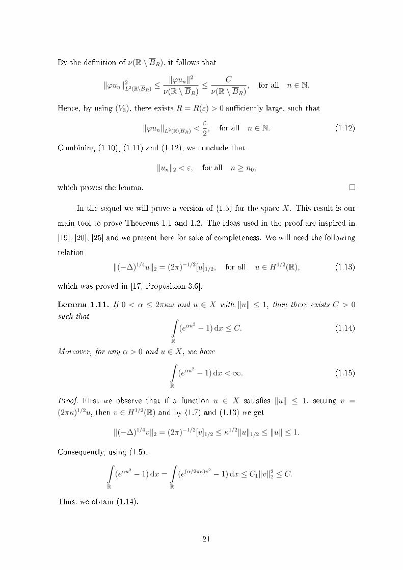
By the denition of ν(R \BR), it follows that

‖ϕun‖2L2(R\BR)

≤ ‖ϕun‖2

ν(R \BR)≤ C

ν(R \BR), for all n ∈ N.

Hence, by using (V3), there exists R = R(ε) > 0 suciently large, such that

‖ϕun‖L2(R\BR) <ε

2, for all n ∈ N. (1.12)

Combining (1.10), (1.11) and (1.12), we conclude that

‖un‖2 < ε, for all n ≥ n0,

which proves the lemma.

In the sequel we will prove a version of (1.5) for the space X. This result is our

main tool to prove Theorems 1.1 and 1.2. The ideas used in the proof are inspired in

[19], [20], [25] and we present here for sake of completeness. We will need the following

relation

‖(−∆)1/4u‖2 = (2π)−1/2[u]1/2, for all u ∈ H1/2(R), (1.13)

which was proved in [17, Proposition 3.6].

Lemma 1.11. If 0 < α ≤ 2πκω and u ∈ X with ‖u‖ ≤ 1, then there exists C > 0

such that ∫R

(eαu2 − 1) dx ≤ C. (1.14)

Moreover, for any α > 0 and u ∈ X, we have∫R

(eαu2 − 1) dx <∞. (1.15)

Proof. First we observe that if a function u ∈ X satises ‖u‖ ≤ 1, setting v =

(2πκ)1/2u, then v ∈ H1/2(R) and by (1.7) and (1.13) we get

‖(−∆)1/4v‖2 = (2π)−1/2[v]1/2 ≤ κ1/2‖u‖1/2 ≤ ‖u‖ ≤ 1.

Consequently, using (1.5),∫R

(eαu2 − 1) dx =

∫R

(e(α/2πκ)v2 − 1) dx ≤ C1‖v‖22 ≤ C.

Thus, we obtain (1.14).

21

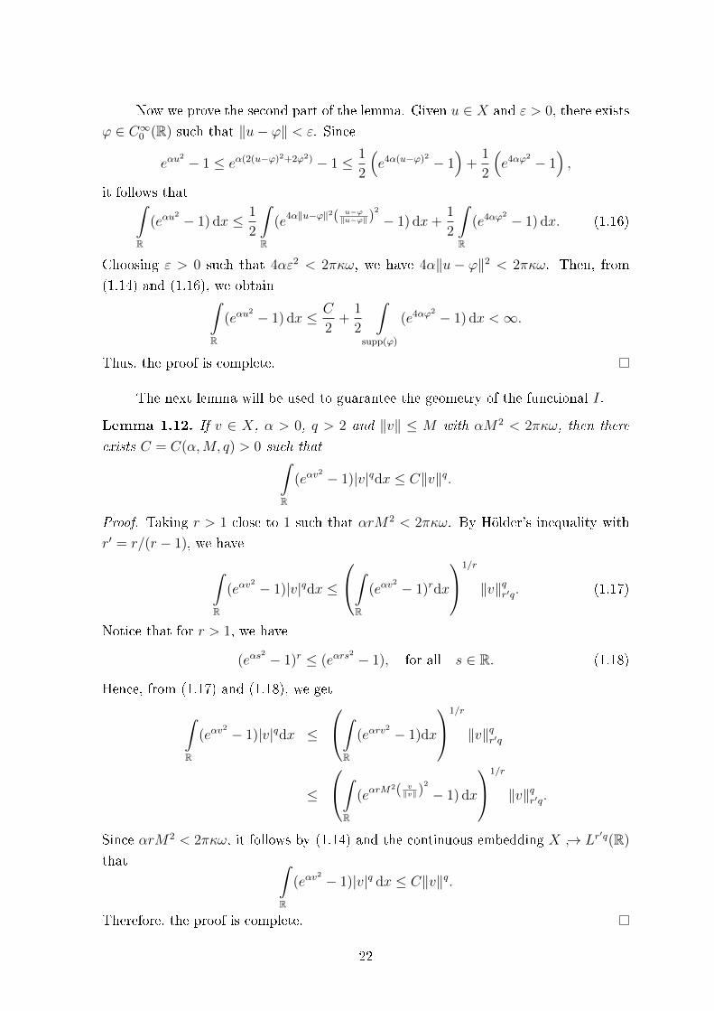
Now we prove the second part of the lemma. Given u ∈ X and ε > 0, there exists

ϕ ∈ C∞0 (R) such that ‖u− ϕ‖ < ε. Since

eαu2 − 1 ≤ eα(2(u−ϕ)2+2ϕ2) − 1 ≤ 1

2

(e4α(u−ϕ)2 − 1

)+

1

2

(e4αϕ2 − 1

),

it follows that∫R

(eαu2 − 1) dx ≤ 1

2

∫R

(e4α‖u−ϕ‖2( u−ϕ‖u−ϕ‖)

2

− 1) dx+1

2

∫R

(e4αϕ2 − 1) dx. (1.16)

Choosing ε > 0 such that 4αε2 < 2πκω, we have 4α‖u− ϕ‖2 < 2πκω. Then, from

(1.14) and (1.16), we obtain∫R

(eαu2 − 1) dx ≤ C

2+

1

2

∫supp(ϕ)

(e4αϕ2 − 1) dx <∞.

Thus, the proof is complete.

The next lemma will be used to guarantee the geometry of the functional I.

Lemma 1.12. If v ∈ X, α > 0, q > 2 and ‖v‖ ≤ M with αM2 < 2πκω, then there

exists C = C(α,M, q) > 0 such that∫R

(eαv2 − 1)|v|qdx ≤ C‖v‖q.

Proof. Taking r > 1 close to 1 such that αrM2 < 2πκω. By Hölder's inequality with

r′ = r/(r − 1), we have∫R

(eαv2 − 1)|v|qdx ≤

∫R

(eαv2 − 1)rdx

1/r

‖v‖qr′q. (1.17)

Notice that for r > 1, we have

(eαs2 − 1)r ≤ (eαrs

2 − 1), for all s ∈ R. (1.18)

Hence, from (1.17) and (1.18), we get∫R

(eαv2 − 1)|v|qdx ≤

∫R

(eαrv2 − 1)dx

1/r

‖v‖qr′q

≤

∫R

(eαrM2( v‖v‖)

2

− 1) dx

1/r

‖v‖qr′q.

Since αrM2 < 2πκω, it follows by (1.14) and the continuous embedding X → Lr′q(R)

that ∫R

(eαv2 − 1)|v|q dx ≤ C‖v‖q.

Therefore, the proof is complete.

22

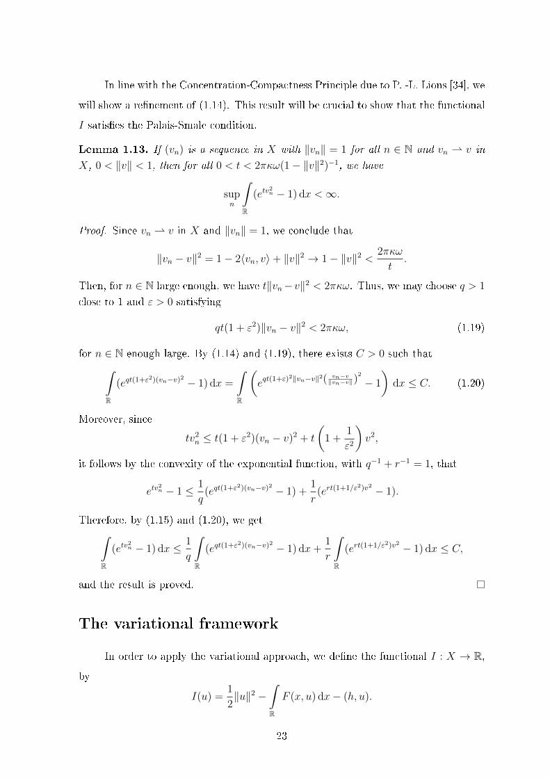
In line with the Concentration-Compactness Principle due to P. -L. Lions [34], we

will show a renement of (1.14). This result will be crucial to show that the functional

I satises the Palais-Smale condition.

Lemma 1.13. If (vn) is a sequence in X with ‖vn‖ = 1 for all n ∈ N and vn v in

X, 0 < ‖v‖ < 1, then for all 0 < t < 2πκω(1− ‖v‖2)−1, we have

supn

∫R

(etv2n − 1) dx <∞.

Proof. Since vn v in X and ‖vn‖ = 1, we conclude that

‖vn − v‖2 = 1− 2〈vn, v〉+ ‖v‖2 → 1− ‖v‖2 <2πκω

t.

Then, for n ∈ N large enough, we have t‖vn−v‖2 < 2πκω. Thus, we may choose q > 1

close to 1 and ε > 0 satisfying

qt(1 + ε2)‖vn − v‖2 < 2πκω, (1.19)

for n ∈ N enough large. By (1.14) and (1.19), there exists C > 0 such that∫R

(eqt(1+ε2)(vn−v)2 − 1) dx =

∫R

(eqt(1+ε)2‖vn−v‖2( vn−v

‖vn−v‖)2

− 1

)dx ≤ C. (1.20)

Moreover, since

tv2n ≤ t(1 + ε2)(vn − v)2 + t

(1 +

1

ε2

)v2,

it follows by the convexity of the exponential function, with q−1 + r−1 = 1, that

etv2n − 1 ≤ 1

q(eqt(1+ε2)(vn−v)2 − 1) +

1

r(ert(1+1/ε2)v2 − 1).

Therefore, by (1.15) and (1.20), we get∫R

(etv2n − 1) dx ≤ 1

q

∫R

(eqt(1+ε2)(vn−v)2 − 1) dx+1

r

∫R

(ert(1+1/ε2)v2 − 1) dx ≤ C,

and the result is proved.

The variational framework

In order to apply the variational approach, we dene the functional I : X → R,

by

I(u) =1

2‖u‖2 −

∫R

F (x, u) dx− (h, u).

23

Notice that, from (f1) and (f2), for each α > α0 and ε > 0, there exists Cε > 0 such

that

|F (x, s)| ≤ (λ1 − ε)2

s2 + Cε(eαs2 − 1), for all s ∈ R,

which combined with the continuous embedding X → L2(R) and (1.15) assures that

F (x, u) ∈ L1(R) for all u ∈ X. Consequently, I is well-dened and, by standard

arguments, I ∈ C1(X,R), (see details in Appendix A), with

I ′(u)v = 〈u, v〉 −∫R

f(x, u)v dx− (h, v),

for all u, v ∈ X. Hence, a critical point of I is a weak solution of (1.1) and reciprocally.

The geometric conditions of the Mountain Pass Theorem for the functional I are

established by the next lemmas.

Lemma 1.14. Suppose that (V1)− (V2) and (f1)− (f2) hold. Then there exists δ1 > 0

such that for each h ∈ X∗ with ‖h‖∗ < δ1, there exists ρh > 0 such that

I(u) > 0 if ‖u‖ = ρh.

Proof. From (f1) and (f2), given ε > 0, there exists C > 0 such that, for all α > α0

and q > 2,

|F (x, s)| ≤ (λ1 − ε)2

s2 + C(eαs2 − 1)|s|q, for all s ∈ R. (1.21)

By using (1.21) and (V2), we reach

I(u) ≥ 1

2‖u‖2 − (λ1 − ε)

2

∫R

u2 dx− C∫R

(eαu2 − 1)|u|q dx− ‖h‖∗‖u‖

≥ 1

2‖u‖2 − (λ1 − ε)

2λ1

‖u‖2 − C∫R

(eαu2 − 1)|u|q dx− ‖h‖∗‖u‖.

Then, for u ∈ X such that α‖u‖2 < 2πκω, using Lemma 1.12, we obtain

I(u) ≥(

1

2− (λ1 − ε)

2λ1

)‖u‖2 − C‖u‖q − ‖h‖∗‖u‖.

Consequently,

I(u) ≥ ‖u‖[(

1

2− (λ1 − ε)

2λ1

)‖u‖ − C‖u‖q−1 − ‖h‖∗

].

Since 12− (λ1−ε)

2λ1> 0, we may choose ρh > 0 such that(

1

2− (λ1 − ε)

2λ1

)ρh − Cρq−1

h > 0.

Thus, for ‖h‖∗ suciently small, there exists ρh such that I(u) > 0 if ‖u‖ = ρh.

Therefore, the proof is complete.

24

Lemma 1.15. Assume that (V1)− (V2) and (f1)− (f3) hold. Then there exists e ∈ Xwith ‖e‖ > ρh such that

I(e) < inf‖u‖=ρh

I(u).

Proof. Let u ∈ C∞0 (R) \ 0, u ≥ 0 with compact support K = supp(u). By using (f2)

and (f3), there exist positive constants C1 and C2 such that

F (x, s) ≥ C1sθ − C2, for all (x, s) ∈ K × [0,∞) and θ > 2.

Then, for t > 0, we get

I(tu) ≤ t2

2‖u‖2 − C1t

θ

∫K

uθ dx+ C2

∫K

dx+ t|(h, u)|.

Since θ > 2, we have I(tu) → −∞ as t → ∞. Setting e = tu with t large enough, we

conclude the proof.

In order to nd an appropriate ball to use minimization argument, we prove the

following result.

Lemma 1.16. Suppose that (V1)−(V2) and (f1)−(f2) hold. If h 6= 0, there exist η > 0

and v ∈ X \ 0 such that I(tv) < 0 for all 0 < t < η. In particular,

−∞ < c0 ≡ inf‖u‖≤η

I(u) < 0.

Proof. For each h ∈ X∗, by applying the Riesz Representation Theorem in the space

X, the problem

(−∆)1/2u+ V (x)u = h, x in R,

has a unique weak solution v ∈ X such that

(h, v) = ‖v‖2 > 0.

Consequently, from (f1) and (f2), there exists η > 0 such that

d

dtI(tv) = t‖v‖2 −

∫R

f(x, tv)v dx− (h, v) < 0,

for all 0 < t < η. Using that I(0) = 0, it must occur I(tv) < 0 for all 0 < t < η, this

concludes the proof.

25

Palais-Smale compactness condition

In this section we will show that the functional I satises the Palais-Smale con-

dition for certain energy levels. Recall that the functional I satises the Palais-Smale

condition at the level c, denoted by (PS)c, if any sequence (un) ⊂ X such that

I(un)→ c and I ′(un)→ 0 as n→∞, (1.22)

has a strongly convergent subsequence in X.

Lemma 1.17. Suppose that (V1)− (V3) and (f1)− (f4) are satised. Let (un) ⊂ X be

an arbitrary Palais-Smale sequence of I at level c. Then there exists a subsequence of

(un) (also denoted by (un)) and u ∈ X such thatun u in X,

f(x, un)→ f(x, u) in L1loc(R),

F (x, un)→ F (x, u) in L1(R).

Proof. By (f3), for θ > 2 we get

I(un)−1

θI ′(un)un =

(1

2− 1

θ

)‖un‖2 +

∫R

(1

θf(x, un)un − F (x, un)

)dx+

(1

θ− 1

)(h, un)

≥(1

2− 1

θ

)‖un‖2 +

(1

θ− 1

)(h, un). (1.23)

Using (1.22), we obtain that for n suciently large

I(un)− 1

θI ′(un)un ≤ C + ‖un‖.

Combining this with (1.23), we have ‖un‖ ≤ C. Since X is a Hilbert space, up to a

subsequence, we may assume that there exists u ∈ X such thatun u in X,

un → u in Lq(R), for all q ∈ [2,∞),

un(x)→ u(x) almost everywhere in R.

From (1.22) and since ‖un‖ ≤ C, there exists C1 > 0 such that∫R

|f(x, un)un| ≤ C1.

Consequently, by [13, Lemma 2.1], we get

f(x, un)→ f(x, u) in L1loc(R), as n→∞. (1.24)

26

Next, similar to N. Lam and G. Lu [30], we will prove the last convergence of the

lemma. Firstly, note that by using (f3) and (f4), for each R > 0, there exists C0 > 0

such that

F (x, un) ≤ C0|f(x, un)|.

This combined with (1.24) and the Generalized Lebesgue's Dominated Convergence

Theorem, imply

F (x, un)→ F (x, u) in L1(BR), for all R > 0.

In order to conclude the last convergence of the lemma, it is sucient to prove that

given δ > 0, there exists R > 0 such that∫BcR

F (x, un) dx ≤ δ and∫BcR

F (x, u) dx ≤ δ.

First, we note that by using (f1), (f3) and (f4), there exist C1, C2 > 0 such that

|F (x, s)| ≤ C1|s|2 + C2|f(x, s)|, for all (x, s) ∈ R× R.

Thus, for each A > 0, we obtain∫|x|>R|un|>A

F (x, un) dx ≤ C1

∫|x|>R|un|>A

|un|2 dx+ C2

∫|x|>R|un|>A

|f(x, un)| dx

≤ C1

A

∫|x|>R|un|>A

|un|3 dx+C2

A

∫R

|f(x, un)un| dx

≤ C1

A‖un‖3 +

C2

A

∫R

|f(x, un)un| dx.

Since ‖un‖ ≤ C and∫R|f(x, un)un| dx ≤ C1, given δ > 0, we may choose A > 0 such

thatC1

A‖un‖3 < δ/3 and

C2

A

∫R

|f(x, un)un| dx < δ/3.

Thus, ∫|x|>R|un|>A

F (x, un) dx ≤ 2δ/3. (1.25)

Now, note that with such A, by (f1) and (f2), we have

F (x, s) ≤ C(α0, A)|s|2, for all (x, s) ∈ R× [−A,A].

27

Then, we get∫|x|>R|un|≤A

F (x, un) dx ≤ C(α0, A)

∫|x|>R|un|≤A

|un|2 dx

≤ 2C(α0, A)

∫|x|>R|un|≤A

|un − u|2 dx+ 2C(α0, A)

∫|x|>R|un|≤A

|u|2 dx.

Hence, by Lemma 1.10, given δ > 0, we may choose R > 0 such that∫|x|>R|un|≤A

F (x, un) dx ≤ δ/3. (1.26)

From (1.25) and (1.26), we have that given δ > 0, there exists R > 0 such that∫|x|>R

F (x, un) dx ≤ δ.

Similarly, ∫|x|>R

F (x, u) dx ≤ δ.

Combining all the above estimates and since δ > 0 is arbitrary, we have∫R

F (x, un) dx→∫R

F (x, u) dx, as n→∞,

which completes the proof.

Finally, let us prove the main result of this section.

Proposition 1.18. Under the hypotheses (V1)− (V3) and (f1)− (f4), if ‖h‖∗ is su-

ciently small then the functional I satises (PS)c for any 0 ≤ c < πκω/α0.

Proof. Let (un) ⊂ X be an arbitrary Palais-Smale sequence of I at the level c. By

Lemma 1.17, up to a subsequence, un u in X. We will show that, up to a subse-

quence, un → u in X. In order to do this, we have two cases to consider:

Case 1: u = 0. In this case, Lemma 1.17, guarantees that∫R

F (x, un)→ 0 and (h, un)→ 0 as n→∞.

Since

c+ on(1) = I(un) =1

2‖un‖2 −

∫R

F (x, un)− (h, un),

28

we get

limn→∞

‖un‖2 = 2c.

Hence, we can infer that for n large there exist r1 > 1 suciently close to 1 and α > α0

close to α0 such that r1α‖un‖2 < 2πκω. Thus, by (1.18) and (1.14),∫R

(eαu2n − 1)r1 dx ≤

∫R

(er1α‖un‖2( un‖un‖)

2

− 1) dx ≤ C. (1.27)

Consequently, ∫R

f(x, un)un dx→ 0 as n→∞.

In fact, since f(x, s) satises (f1) and (f2), for α > α0 and ε > 0, there exists C1 > 0

such that

|f(x, s)| ≤ (λ1 − ε)|s|+ C1(eαs2 − 1), for all s ∈ R.

Letting r1 > 1 close to 1 such that r2 ≥ 2, where 1/r1 +1/r2 = 1, we obtain by Hölder's

inequality that∣∣∣∣∣∣∫R

f(x, un)un dx

∣∣∣∣∣∣ ≤ C

∫R

|un|2 dx+C

∫R

(eαu2n − 1)r1 dx

1/r1∫R

|un|r2 dx

1/r2

→ 0,

where we have used (1.27) and Lemma 1.10. Therefore, since I ′(un)un = on(1), we

conclude that, up to a subsequence, un → 0 in X.

Case 2: u 6= 0. In this case, since (un) is a Palais-Smale sequence of I at the level c,

we may dene

vn =un‖un‖

and v =u

lim ‖un‖.

It follows that vn v in X, ‖vn‖ = 1 and ‖v‖ ≤ 1. If ‖v‖ = 1, we conclude the

proof. If ‖v‖ < 1, we claim that there exist r1 > 1 suciently close to 1, α > α0 close

to α0 and β > 0 such that

r1α‖un‖2 ≤ β < 2πκω(1− ‖v‖2)−1 (1.28)

for n ∈ N large. In fact, since I(un) = c+ on(1), it follows that

1

2limn→∞

‖un‖2 = c+

∫R

F (x, u) dx+ (h, u). (1.29)

Setting

A =

c+

∫R

F (x, u) dx+ (h, u)

(1− ‖v‖2),

29

from (1.29) and by the denition of v, we obtain

A = c− I(u),

which together with (1.29) imply

1

2limn→∞

‖un‖2 =A

1− ‖v‖2=c− I(u)

1− ‖v‖2. (1.30)

Note that

c− I(u) < c+1

2(h, u). (1.31)

Indeed, since the norm is lower semicontinuous, from (1.29) it follows that I(u) ≤ c.

Moreover, for all ϕ ∈ C∞0 (R),

I ′(un)ϕ = 〈un, ϕ〉 −∫R

f(x, un)ϕ dx− (h, ϕ).

Since un u in X, passing to the limit in the above equality, by Lemma 1.17, we have

I ′(u)ϕ = 〈u, ϕ〉 −∫R

f(x, u)ϕ dx− (h, ϕ) = 0,

for all ϕ ∈ C∞0 (R). By density, we conclude that I ′(u)v = 0 for all v ∈ X. In particular,

I ′(u)u = 0. Thus, from (f3) we obtain

0 = I ′(u)u = ‖u‖2 −∫R

f(x, u)u dx− (h, u)

< 2

1

2‖u‖2 −

∫R

F (x, u) dx− (h, u)

+ (h, u)

= 2I(u) + (h, u),

which implies (1.31).

Now, note that

‖u‖ ≤(θ − 1)‖h‖∗ +

√(1− θ)2‖h‖2

∗ + 2θc(θ − 2)

(θ − 2). (1.32)

Indeed, since I(u) ≤ c and I ′(u)u = 0, we have

θI(u)− I ′(u)u =

(θ

2− 1

)‖u‖2 +

∫R

[f(x, u)u− θF (x, u)] dx+ (1− θ)(h, u) ≤ θc.

Thus, from (f3), we have(θ − 2

2

)‖u‖2 + (1− θ)‖h‖∗‖u‖ − θc ≤ 0.

30

Consequently, (1.32) holds. Therefore, from (1.30), (1.31) and (1.32) for ‖h‖∗ su-

ciently small, we conclude

1

2limn→∞

‖un‖2 =c− I(u)

1− ‖v‖2<

πκω

α0(1− ‖v‖2)(1.33)

Consequently, (1.28) holds. By (1.18) and Lemma 1.13, we get∫R

(eαu2n − 1)r1 dx ≤ C.

By Hölder's inequality and similar computations done above we obtain∫R

f(x, un)(un − u) dx→ 0 as n→∞.

This convergence and the fact that I ′(un)(un − u) = on(1), imply that

‖un‖2 = (un, u) + on(1).

Since un u in X, we obtain un → u in X and the proof is nished.

Proposition 1.19. Under the hypotheses (V1)− (V3) and (f1)− (f4), if ‖h‖∗ is su-

ciently small then the functional I satises (PS)c0.

Proof. Let (un) ⊂ Bρh be an arbitrary Palais-Smale sequence of I at the level c0. By

the Lemma 1.17, up to a subsequence, un u in X. We will show that, up to a

subsequence, un → u in X. Note that∫R

f(x, un)(un − u)dx→ 0 as n→∞. (1.34)

Firstly, since ‖un‖ ≤ ρh making ρh suciently small, taking r1 > 1 suciently close to

1 and α suciently close to α0 we may infer that r1α‖un‖2 < 2πκω. Thus, by (1.18)

and (1.14), ∫R

(eαu2n − 1)r1 dx ≤

∫R

(er1α‖un‖2( un‖un‖)

2

− 1) dx ≤ C. (1.35)

Moreover, since f(x, s) satises (f1) and (f2), for α > α0 and ε > 0, there exists C1 > 0

such that

|f(x, s)| ≤ (λ1 − ε)|s|+ C1(eαs2 − 1), for all s ∈ R.

Letting r1 > 1 close to 1 such that r2 ≥ 2, where 1/r1 +1/r2 = 1, we obtain by Hölder's

inequality that∣∣∣∣∣∣∫R

f(x, un)(un − u) dx

∣∣∣∣∣∣ ≤ C

∫R

|un|2 dx

1/2∫R

(un − u)2 dx

1/2

+ C

∫R

(eαu2n − 1)r1 dx

1/r1∫R

(un − u)r2 dx

1/r2

→ 0,

31

where we have used (1.35) and Lemma 1.10. Therefore, this convergence and the fact

that I ′(un)(un − u) = on(1), imply that

‖un‖2 = (un, u) + on(1).

Since un u in X, we conclude that, up to a subsequence, un → u in X.

Estimate of the minimax level

In this section we will prove an estimate for the minimax level. First, we will

need the following lemma.

Lemma 1.20. Suppose that (V1)− (V3) hold. Then Sp given in (1.9) is attained by a

nonnegative function up ∈ X.

Proof. Let (un) be a minimizing sequence of nonnegative functions (if necessary, replace

un by |un|, which is possible since by using the triangle inequality we have |un(x) −un(y)| ≥ ||un(x)| − |un(y)||) for Sp in X, that is,

‖un‖p = 1 and

1

2π

∫R2

(un(x)− un(y))2

|x− y|2dx dy +

∫R

V (x)u2n dx

1/2

→ Sp.

Then, (un) is bounded in X. Since X is a Hilbert space and X is compactly embedded

into Lp(R), up to a subsequence, we may assume

un up in X,

un → up in Lp(R),

un(x)→ up(x) almost everywhere in R.

Consequently, ‖up‖p = 1,

‖up‖ ≤ lim infn→+∞

‖un‖ = Sp,

up(x) ≥ 0 almost everywhere in R.

Thus, Sp = ‖up‖. This completes the proof.

Now we prove the main result of this section.

Lemma 1.21. Suppose that (V1) − (V3) and (f5) are satised, if ‖h‖∗ is suciently

small then

maxt≥0

I(tup) <πκω

α0

.

32

Proof. Let Ψ : [0,+∞)→ R, given by

Ψ(t) =t2

2

1

2π

∫R2

(up(x)− up(y))2

|x− y|2dxdy +

∫R

V (x)u2p dx

− ∫R

F (x, tup) dx.

By Lemma 1.20 and (f5), we have

Ψ(t) ≤ t2

2S2p −

Cpptp ≤ max

t≥0

[t2

2S2p −

Cpptp]

=(p− 2)

2p

S2p/(p−2)p

C2/(p−2)p

<πκω

α0

. (1.36)

To conclude, notice that t|(h, up)| ≤ t‖h‖∗‖up‖ with t in a compact interval. Therefore,

taking ‖h‖∗ suciently small and using (1.36) the result follows.

Proofs of Theorem 1.1 and 1.2

Initially, it follows from Lemma 1.14 and Lemma 1.15 that the functional I sa-

tises the geometric conditions of the Mountain Pass Theorem. Consequently, the

minimax level

cm = infg∈Γ

maxt∈[0,1]

I(g(t))

is positive, where Γ = g ∈ C([0, 1], X) : g(0) = 0, g(1) = e.

On the other hand, by Lemma 1.21 and Proposition 1.18, the functional I satises

the (PS)cm condition. Thus, by the Mountain Pass Theorem the functional I has a

critical point um at the minimax level cm.

Moreover, when h ∈ X∗ with h 6≡ 0, we may nd a second solution. In order

to do this, we consider ρh like in Lemma 1.14 and we observe that Bρh is a convex

complete metric space with the metric induced by the norm of X, and the functional

I is C1 and bounded below on Bρh . Hence, by the Ekeland variational principle there

exists a sequence (un) in Bρh such that

I(un)→ c0 < 0 and ‖I ′(un)‖∗ → 0.

By the Proposition 1.19, the functional I satises the (PS)c0 condition. Consequently,

the functional I has a critical point u at the level c0. Therefore, the proof of the results

is complete.

33

Chapter 2

On nonlinear perturbations of a

periodic fractional Schrödinger

equation with critical exponential

growth

In this chapter we present the results of the paper [15], more specically, we study

the existence of solutions for fractional Schrödinger equations of the form

(−∆)1/2u+ V (x)u = f(x, u) in R,

where V is a bounded potential, which belongs to a dierent class of those treated

in Chapter 1, and the nonlinear term f(x, u) is considered with critical exponen-

tial growth. We prove the existence of a nontrivial weak solution by combining the

Mountain Pass Theorem, Trudinger-Moser's inequality and a version of Concentration-

Compactness Principle due to Lions.


As mentioned in the introduction, some results have appeared, recently, in the

literature concerning the equation

(−∆)1/2u+ V (x)u = f(x, u) in R, (2.1)

34

with interesting conditions on V (x) and f(x, u). The main purpose of this chapter is to

study (2.1) considering the nonlinearity with exponential growth. As we have seen in

Chapter 1, the Sobolev embedding states that H1/2(R) → Lq(R) for any q ∈ [2,+∞),

but H1/2(R) is not continuous embedded in L∞(R) (for details see [17, 39]). Thus the

maximal growth, which allows us to treat (2.1) variationally in H1/2(R), is motivated

by Trudinger-Moser's inequality proved by T. Ozawa [39] and H. Kozono, T. Sato and

H. Wadade [29]. More precisely, they proved that there exist positive constants ω and

C = C(ω) such that, for all u ∈ H1/2(R) with ‖(−∆)1/4u‖2 ≤ 1,∫R(eαu

2 − 1) dx ≤ C‖u‖22, for all α ∈ (0, ω]. (2.2)

Therefore, the maximal growth on the nonlinearity f(x, u), that allows us to treat (2.1)

variationally in H1/2(R), is given by eα0u2 when |u| → +∞ for some α0 > 0 (see also

the pioneers works [38,45]).

Motivated by Trudinger-Moser inequality (2.2) and by the works [1,14,23,25], we

deal with two problems. First, we investigate (2.1) when V (x) and f(x, u) are periodic

functions with respect to x, and f(x, u) behaves like eα0u2 when |u| → +∞ for some

α0 > 0. Second, with the aid of the previous case, we study a more general problem

assuming that V (x) and f(x, u) are just asymptotically periodic at innity. Next, for

easy reference, we recall the problems and assumptions.

A periodic problem

The rst problem that we will study in this chapter is the following, (−∆)1/2u+ V0(x)u = f0(x, u) in R,

u ∈ H1/2(R) and u ≥ 0,(P0)

where (−∆)1/2 is dened, for a suciently regular function, by

(−∆)1/2u(x) = − 1

2π

∫R

u(x+ y) + u(x− y)− 2u(x)

|y|2dy. (2.3)

The assumptions on the functions V0(x) and f0(x, u) are the following: V0 : R →

(0,+∞) is a continuous 1−periodic function and f0 : R × R → R is a continuous

1−periodic function in x, which has critical exponential growth in u, that is, there

35

exists α0 > 0 such that

lim|s|→+∞

f0(x, s)e−αs2

=

0, for all α > α0,

+∞, for all α < α0,

(2.4)


Recall that this notion of criticality is directed by (2.2) and it has been used in

several papers involving exponential growth, see for instance [13], [20] and [25]. Since

we are interested in the existence of nonnegative solutions, we set f0(x, s) = 0 for

all (x, s) ∈ R × (−∞, 0]. We also assume that the nonlinearity f0(x, u) satises the

conditions

(f0,1) lims→0

f0(x, s)


(f0,2) there exists a constant θ > 2 such that

0 < θF0(x, s) := θ

s∫0

f0(x, t) dt ≤ sf0(x, s) for all (x, s) ∈ R× (0,+∞);

(f0,3) for each xed x ∈ R, the function f0(x, s)/s is increasing with respect to s ∈ R;

(f0,4) there are constants p > 2 and Cp > 0 such that

f0(x, s) ≥ Cpsp−1, for all (x, s) ∈ R× [0,+∞),

where

Cp >

[(p− 2)θα0

(θ − 2)pω

](p−2)/2

Spp (2.5)

and

Sp := infu∈H1/2(R)‖u‖p=1

1

2π

∫R2

|u(x)− u(y)|2

|x− y|2dxdy + ‖V ‖∞

∫R

u2 dx

1/2

.

Throughout this chapter, we say that u ∈ H1/2(R) is a weak solution for (P0) ifthe following equality holds:

1

2π

∫R2

(u(x)− u(y))(v(x)− v(y))|x− y|2

dx dy+

∫R

V0(x)uv dx =

∫R

f0(x, u)v dx, for all v ∈ H1/2(R).

Under these conditions we have the rst result of this chapter:

36

Theorem 2.1. Assume that (f0,1)−(f0,4) hold. Then (P0) has a nonnegative nontrivial

weak solution.

As a consequence of this theorem we nd a nonnegative nontrivial weak solution

for the following model problem:

(−∆)1/2u+ u = G′0(u) in R,

with G0(u) = Cppup eα0u2 , u ≥ 0, p > 2 and Cp as dened in (2.5).

An asymptotically periodic problem

The second problem that we will study in this chapter is the following, (−∆)1/2u+ V (x)u = f(x, u) in R,

u ∈ H1/2(R) and u ≥ 0.(P )

Next we will describe the conditions on the functions V (x) and f(x, s) in a more

precise way.

(V1) V : R→ [0,+∞) is a continuous function satisfying the conditions: V (x) ≤ V0(x)

for any x ∈ R and V0(x)− V (x)→ 0 as |x| → ∞;

We assume that the nonlinearity f : R×R→ R is a continuous function satisfying

(2.4), f(x, s) = 0 for all (x, s) ∈ R× (−∞, 0] and also the following conditions:

(f1) f(x, s) ≥ f0(x, s) for all (x, s) ∈ R× [0,+∞), and for all ε > 0, there exists η > 0

such that for s ≥ 0 and |x| ≥ η,

|f(x, s)− f0(x, s)| ≤ εeα0s2 ;

(f2) lims→0

f(x, s)


(f3) there exists a constant µ > 2 such that

0 < µF (x, s) := µ

s∫0

f(x, t) dt ≤ sf0(x, s), for all (x, s) ∈ R× (0,+∞);

(f4) for each xed x ∈ R, the function f(x, s)/s is increasing with respect to s ∈ R;

37

(f5) at least one of the nonnegative continuous functions V0(x)− V (x) and f(x, s)−

f0(x, s) is positive on a set of positive measure.

We say that u ∈ H1/2(R) is a weak solution for (P ) if the following equality holds:

1

2π

∫R2

(u(x)− u(y))(v(x)− v(y))|x− y|2

dx dy+

∫R

V (x)uv dx =

∫R

f(x, u)v dx, for all v ∈ H1/2(R).

The second result of this chapter is the following:

Theorem 2.2. Assume that (V1) and (f1) − (f5) hold. Then (P ) has a nonnegative

nontrivial weak solution.

As mentioned earlier, the results of this chapter were motivated by the works

[1, 14, 23, 25]. Particularly, J. M. do Ó et al. in [23] have proved the existence of a

nontrivial solution for the fractional Schrödinger equation

(−∆)1/2u+ u = K(x)g(u) in R,

where g(u) behaves like eα0u2 when |u| → +∞ for some α0 > 0 and K : R → R is a

positive function such that K ∈ L∞(R) ∩C(R). Furthermore, if An is a sequence of

Borel sets of R with |An| ≤ R for some R > 0,

limr→∞

∫An∩Bc(0,R)

K(x)dx = 0, uniformly with respect to n ∈ N.

We were inspired by Alves et al. [1], thus we studied (P ) assuming that the

potential V (x) and the nonlinearity f(x, u) are asymptotically periodic at innity. Here

we work with a general class of functions which are asymptotic to a nonautonomous

periodic function at innity. In this sense our work completes the study presented

in [22, 23]. It complements also [10, 11, 18, 41] since we consider the limiting case for

N = 1 and s = 1/2 when the nonlinearity has exponential growth in the sense of the

Trudinger-Moser inequality. Moreover, also complements the study of Chapter 1 since

we consider that the potential V (x) belongs to a dierent class from those treated

there.

Remark 2.3. The assumptions on the nonlinearity and the potential are standard,

since we use a variational approach. Notice that our assumptions assure the mountain

pass geometry of the functionals I0 and I (which are dened in Sections 2 and 2).

Furthermore, by (V1) the potential V (x) may be zero on bounded sets. For more

details see Lemma 2.6.

38

Remark 2.4. As examples of functions that veries our assumptions we may consider

V (x) = 2 +|x|2

|x|2 + 1| sin(x)| with V0(x) = 2 + | sin(x)|, or

V (x) =

0, if x2 ≤ 1

x2 − 1, if 1 ≤ x2 ≤ 4

3, if x2 ≥ 4

with V0(x) ≡ 3.

Remark 2.5. We highlight that when u has sucient regularity, it is possible to have a

pointwise expression of the fractional Laplacian as (2.3) (see [47], for example). Again

in this case we have u > 0 if u 6= 0, (see Remark 3.4).

To prove our main theorems we have used variational methods. An important

point is a version of a Concentration-Compactness Principle. This one is crucial to show

that Sp is attained and that the weak limit of an appropriate Palais-Smale sequence is

nontrivial.

The outline of this chapter is as follows: Section 2.2 contains some preliminary

results. Section 2.3 and Section 2.4 deal with the proof of Theorems 2.1 and 2.2,

respectively.

Some preliminary results

In this section, we prove some technical results and we establish the appropriate

setting to prove Theorems 2.1 and 2.2.

The functional setting

In order to study variationally (P ) we consider a suitable subspace of the frac-

tional Sobolev space H1/2(R), which is dened by

H1/2(R) :=

u ∈ L2(R) :

|u(x)− u(y)||x− y|

∈ L2(R× R)

,

endowed with the natural norm

‖u‖1/2 := ([u]21/2 + ‖u‖22)1/2,

where the term

[u]1/2 :=

(∫R2

|u(x)− u(y)|2

|x− y|2dx dy

)1/2

39

is the so-called Gagliardo semi-norm of function u.

Recall that H1/2(R) is a Hilbert space and by [17, Proposition 3.6]

‖(−∆)1/4u‖2 = (2π)−1/2[u]1/2 for all u ∈ H1/2(R). (2.6)

The next lemma provides an inequality that we will use in some proofs.

Lemma 2.6. Suppose that (V1) holds. Then there exists a constant κ > 0 satisfying

1

2π

∫R2

|u(x)− u(y)|2

|x− y|2dxdy +

∫R

V (x)u2 dx ≥ κ‖u‖22 for all u ∈ H1/2(R). (2.7)

Proof. Suppose that (2.7) does not hold. Then for each n ∈ N there exists un ∈ H1/2(R)

such that

‖un‖2 = 1 and1

2π

∫R2

(un(x)− un(y))2

|x− y|2dx dy

+

∫R

V (x)u2n dx <

1

n. (2.8)

Since V (x) ≥ 0, we get that [un]21/2 → 0, (un) is bounded in H1/2(R) and, up to a

subsequence,

un u0 in H1/2(R), as n→∞. (2.9)

We also have that ∫R

V (x)u2n dx→ 0, as n→∞. (2.10)

Now, we use the following inequality, proved in [39, p.261], given by

‖un‖r ≤ C‖(−∆)1/4un‖1−θ2 ‖un‖θ2,

where r > 2, C > 0 and θ ∈ (0, 1). This inequality together with (2.6) implies

‖un‖r ≤ C[un](1−θ)1/2 ‖un‖

θ2,

from which it follows that ‖un‖r → 0. On the other hand, by (2.9) un → u0 in Lrloc(R).

Consequently, u0 ≡ 0.

From (2.8), for each R > 0 we can write

1 =

∫R

u2n dx =

∫BR

u2n dx+

∫BcR

u2n dx. (2.11)

Next, in order to reach a contradiction we will use (V1). More precisely, given ε > 0,

there exists R > 0, such that

V0(x)− V (x) ≤ ε for all x ∈ BcR.

40

Thus, for all x ∈ BcR and ε > 0 suciently small,

V (x) ≥ V0(x)− ε ≥ C0 − ε = b0 > 0. (2.12)

Combining (2.11), (2.12), (2.10) and the fact that un → 0 in L2(BR), we obtain the

contradiction

1 ≤∫BR

u2n dx+

1

b0

∫BcR

V (x)u2n dx→ 0.

Therefore, (2.7) holds and the lemma is proved.

We will use the following notations: X0 will denote H1/2(R) endowed with the

equivalent norm

‖u‖X0 =

1

2π

∫R2

|u(x)− u(y)|2

|x− y|2dx dy

+

∫R

V0(x)u2 dx

1/2

and X1 will denote H1/2(R) endowed with the norm

‖u‖X1 =

1

2π

∫R2

|u(x)− u(y)|2

|x− y|2dx dy

+

∫R

V (x)u2 dx

1/2

.

As consequence of inequality (2.7) we have that ‖ · ‖X1 is a norm and also that

the embedding X1 → Lq(R) is continuous for all 2 ≤ q <∞.

Trudinger-Moser type inequalities

In this subsection we prove a version of (2.2) to the space H1/2(R) with the norms

‖ · ‖X0 and ‖ · ‖X1 . This will be our principal tool to prove our main results. The ideas

used in the proof are inspired in [19,20,25] and we present them here for completeness

of our work.

Lemma 2.7. If 0 < α < ω, then there exists a constant C = C(ω) > 0, such that

supu∈H1/2(R) : ‖u‖Xi≤1

∫R

(eαu2 − 1) dx ≤ C for i = 0, 1. (2.13)

Moreover, for any α > 0 and u ∈ H1/2(R) we have∫R

(eαu2 − 1) dx <∞. (2.14)

41

Proof. First, we observe that if a function u ∈ H1/2(R) satises ‖u‖Xi ≤ 1, then by

using (2.6), we get

‖(−∆)1/4u‖2 = (2π)−1/2[u]1/2 ≤ ‖u‖Xi ≤ 1.

Consequently, ∫R

(eαu2 − 1) dx ≤ C1‖u‖2

2 ≤ C,

where we have used (2.2) and (2.7). Thus, we obtain (2.13).

Now we prove the second part of the lemma. Given u ∈ H1/2(R) and ε > 0 there

exists ϕ ∈ C∞0 (R) such that ‖u− ϕ‖Xi < ε. Since

eαu2 − 1 ≤ eα(2(u−ϕ)2+2ϕ2) − 1 ≤ 1

2

(e4α(u−ϕ)2 − 1

)+

1

2

(e4αϕ2 − 1

),

it follows that∫R

(eαu2 − 1) dx ≤ 1

2

∫R

(e4α‖u−ϕ‖2Xi

(u−ϕ

‖u−ϕ‖Xi

)2

− 1) dx+1

2

∫R

(e4αϕ2 − 1) dx. (2.15)

Choosing ε > 0 such that 4αε2 < ω, we have 4α‖u− ϕ‖2Xi< ω. Then, from (2.13) and

(2.15), it follows that∫R

(eαu2 − 1) dx ≤ C

2+

1

2

∫supp(ϕ)

(e4αϕ2 − 1) dx <∞.

This completes the proof of the lemma.

Lemma 2.8. If α > 0, q > 2, v ∈ Xi and ‖v‖Xi ≤M with αM2 < ω, then there exists

C = C(α,M, q) > 0, such that∫R

(eαv2 − 1)|v|qdx ≤ C‖v‖qXi for i = 0, 1.

Proof. Consider r > 1 close to 1 such that αrM2 < ω. Using Hölder's inequality with

r′ = r/(r − 1), we have

∫R

(eαv2 − 1)|v|qdx ≤

∫R

(eαv2 − 1)rdx

1/r

‖v‖qr′q. (2.16)

Notice that given r > 1 for all s ∈ R,

(eαs2 − 1)r ≤ (eαrs

2 − 1). (2.17)

42

Hence, from (2.16) and (2.17) we get

∫R

(eαv2 − 1)|v|qdx ≤

∫R

(eαrv2 − 1)dx

1/r

‖v‖qr′q

≤

∫R

(eαrM2

(v

‖v‖Xi

)2

− 1) dx

1/r

‖v‖qr′q.

Thus, since αrM2 < ω, it follows from (2.13) and the continuous embedding Xi →Lr′q(R) that ∫

R

(eαv2 − 1)|v|q dx ≤ C‖v‖qXi ,

which proves the lemma.

A Concentration-Compactness Principle

The next lemma is a version of a Lions's result (see P. L. Lions [35]).

Lemma 2.9. If (uk) is bounded in H1/2(R) and

limk→∞

supy∈R

∫BR(y)

|uk(x)|2 dx = 0, (2.18)

for some R > 0, then uk → 0 in Lq(R) for 2 < q <∞.

Proof. For each r > q, by standard interpolation, we obtain

‖uk‖Lq(BR(y)) ≤ ‖uk‖1−λL2(BR(y))‖uk‖

λLr(BR(y)),

where (1− λ)/2 + λ/r = 1/q with 0 < λ < 1. Covering R by balls of radius R, in such

way that each point of R is contained in at most 2 balls, we nd C > 0 such that

‖uk‖qLq(R) ≤ C supy∈R

∫BR(y)

|uk|2 dx

(1−λ)q/2

‖uk‖λqLr(R).

By the continuous embedding H1/2(R) → Lr(R) and ‖uk‖1/2 ≤ C1, we get

∫R

|uk|q dx ≤ C supy∈R

∫BR(y)

|uk|2 dx

(1−λ)q/2

and so by (2.18) we conclude the proof.

Using the previous lemma, we obtain the following result.

43

Lemma 2.10. The constant Sp is attained by a nonnegative function up ∈ H1/2(R).

Proof. Let (ϑk) be a minimizing sequence of nonnegative functions for Sp in H1/2(R)

(if necessary, replace ϑk by |ϑk|, which is possible since by using the triangle inequality

we have |ϑk(x)− ϑk(y)| ≥ ||ϑk(x)| − |ϑk(y)||), that is,

∫R

|ϑk|p dx = 1 and

1

2π

∫R2

(ϑk(x)− ϑk(y))2

|x− y|2dx dy + ‖V ‖∞

∫R

ϑ2k dx

1/2

→ Sp.

Here, we consider H1/2(R) endowed with the norm

‖u‖ =

1

2π

∫R2

|u(x)− u(y)|2

|x− y|2dxdy + ‖V ‖∞

∫R

u2 dx

1/2

.

It is clear that ‖ϑk‖ ≤ C for some C > 0. Then, up to a subsequence, we may assume

that ϑk ϑ in H1/2(R) and

‖ϑ‖ ≤ lim infk→+∞

‖ϑk‖ = Sp.

Then ϑ is a minimizer provided that ‖ϑ‖p = 1. But we know only that ‖ϑ‖p ≤ 1.

Notice that, since ‖ϑk‖p = 1, Lemma 2.9 implies

δ = limk→∞

supy∈R

∫B1(y)

|ϑk(x)|2dx > 0.

Thus, up to a subsequence, we may assume the existence of (yk) ⊂ R such that∫B1(yk)

|ϑk(x)|2dx > δ/2.

Let us dene uk(x) := ϑk(x+ yk). Hence, ‖uk‖p = ‖ϑk‖p = 1, ‖uk‖ = ‖ϑk‖ → Sp and∫B1(0)

|uk(x)|2dx > δ/2. (2.19)

Since (uk) is bounded in H1/2(R), we may assume, up to a subsequence,uk up in H1/2(R),

uk → up in L2loc(R),

uk → up almost everywhere in R.

By the Brézis-Lieb Lemma (see [7]), we have that

1 = ‖up‖pp + limk→∞‖uk − up‖pp and lim

k→∞‖uk‖2 = ‖up‖2 + lim

k→∞‖uk − up‖2.

44

Thus, we have

S2p = lim

k→∞‖uk‖2 = ‖up‖2 + lim

k→∞‖uk − up‖2

≥ S2p [(‖up‖pp)2/p + (1− ‖up‖pp)2/p].

(2.20)

By (2.19), we have up 6= 0. If we suppose by contradiction that ‖up‖p < 1, by using

(2.20) follows that

S2p > S2

p(‖up‖pp + 1− ‖up‖pp)2/p,

what is a contradiction. Therefore, ‖up‖p = 1 and up is a minimizer for Sp, and this

completes the proof.

Existence of a solution for the periodic problem

In order to apply the Mountain Pass Theorem without the Palais-Smale condition

(see [37, Theorem 4.3]) to nd a nontrivial solution for the problem (P0), we will

consider the functional I0 : X0 → R given by

I0(u) =1

2‖u‖2

X0−∫R

F0(x, u) dx.

Notice that I0 is well dened. Indeed, combining the condition (f0,1) and the fact

that f0(x, s) has critical exponential growth, for each α > α0 and ε > 0 there exists a

positive constant Cε such that

F0(x, s) ≤ ε

2s2 + Cε(e

αs2 − 1) for all (x, s) ∈ R× R.

Combining this estimate together with the continuous embedding X0 → L2(R) and

(2.14), we obtain that F0(x, u) ∈ L1(R) for all u ∈ X0. Hence, I0 is well dened.

By using standard arguments we can see that I0 ∈ C1(X0,R), see Appendix A,

with

I ′0(u)φ =1

2π

∫R2

(u(x)− u(y))(φ(x)− φ(y))

|x− y|2dx dy +

∫R

V0(x)uφ dx−∫R

f0(x, u)φ dx,

for all φ ∈ X0. Therefore, a critical point of I0 is a weak solution of (P0) and recipro-

cally.

Now we prove some facts about the geometric structure of I0 required by the

minimax procedure.

45

Lemma 2.11. Suppose that (f0,1) is satised. Then there exist ρ, σ > 0 such that

I0(u) ≥ σ if ‖u‖X0 = ρ.

Proof. Combining (f0,1) and the fact that f0(x, s) has critical exponential growth, for

each α > α0, q > 2 and ε > 0 there exists Cε > 0 such that

F0(x, s) ≤ ε

2s2 + Cε|s|q(eαs

2 − 1) for all (x, s) ∈ R× R. (2.21)

From (2.21) and the continuous embedding X0 → L2(R), we obtain

I0(u) ≥ 1

2‖u‖2

X0− ε

2‖u‖2

2 − Cε∫R

(eαu2 − 1)|u|q dx

≥(

1

2− εC1

2

)‖u‖2

X0− Cε

∫R

(eαu2 − 1)|u|q dx.

Then, for each u ∈ X0 with α‖u‖2X0< ω, by applying Lemma 2.8, we get

I0(u) ≥(

1

2− εC1

2

)‖u‖2

X0− C2‖u‖qX0

= ‖u‖2X0

[(1

2− εC1

2

)− C2‖u‖q−2

X0

].

Since q > 2, we may choose ε > 0 and ρ > 0 suciently small such that(1

2− εC1

2

)− C2ρ

q−2 > 0.

Thus, there exist ρ, σ > 0 such that I0(u) ≥ σ if ‖u‖X0 = ρ, which is the desired

conclusion.

Lemma 2.12. Suppose that (f0,2) is satised. Then there exists e ∈ X0 with ‖e‖X0 > ρ

such that

I0(e) < inf‖u‖X0

= ρI0(u).

Proof. Let u ∈ C∞0 (R)\0 with support K. By (f0,2) there exist C1, C2 > 0 such that

F0(x, u) ≥ C1|u|θ − C2 for all x ∈ K.

Consequently, we have the following estimate for t > 0,

I0(tu) ≤ t2

2‖u‖2

X0− C1t

θ

∫K

|u|θ dx+ C2

∫K

dx.

Since θ > 2, we obtain I0(tu) → −∞ as t → ∞. Setting e = tu with t large enough,

we conclude the proof.

46

Minimax level

As a consequence of Lemmas 2.11 and 2.12, the minimax level

c0 = infg∈Γ

maxt∈[0,1]

I0(g(t))

is positive, where Γ = g ∈ C([0, 1], X0) : g(0) = 0 and g(1) = e.

Next, we provide an estimate to the minimax level.

Lemma 2.13. Suppose that (f0,4) holds. Then

σ ≤ c0 <(θ − 2)ω

2θα0

.

Proof. Applying Lemma 2.11 we have that c0 ≥ σ. In order to get an upper estimate,

we consider the function uq given in Lemma 2.10. Thus, it follows that

c0 ≤ maxt≥0

I0(tuq)

≤ maxt≥0

[t2

2‖uq‖2 − Cq

qtq‖uq‖qq

]= max

t≥0

[t2

2S2q −

Cqqtq]

=(q − 2)

2q

S2q/(q−2)q

C2/(q−2)q

<(θ − 2)ω

2θα0

,

where we have used (f0,4). This completes the proof of the lemma.

On Palais-Smale sequences

By the Mountain Pass Theorem without the (PS) condition (see [37, Theorem

4.3]), there exists a sequence (uk) in X0 satisfying

I0(uk)→ c0 and I ′0(uk)→ 0. (2.22)

Lemma 2.14. Suppose that (f0,1) and (f0,2) hold. Then the sequence (uk) is bounded

in X0 and its weak limit denoted by u0 is a weak solution of (P0).

Proof. Using well-known arguments it is not dicult to check that (uk) is a bounded

sequence in X0. Indeed, by (f0,2) we have

I0(uk)−1

θI ′0(uk)uk =

(1

2− 1

θ

)‖uk‖2

X0+

∫R

[1

θf0(x, uk)uk − F0(x, uk)

]dx

≥(

1

2− 1

θ

)‖uk‖2

X0.

(2.23)

47

By (2.22), there exists k0 ∈ N such that for all k ∈ N with k ≥ k0, it holds

I0(uk)−1

θI ′0(uk)uk ≤ C + ‖uk‖X0 .

This together with (2.23) imply that ‖uk‖X0 ≤ C1.

Since X0 is a Hilbert space, up to a subsequence, we can assume that there exists

u0 ∈ X0 such that uk u0 in X0,

uk → u0 in Lqloc(R) for all q ≥ 1,

uk(x)→ u0(x) almost everywhere in R.

In order to complete the proof of the lemma, it is sucient to prove that∫R

f0(x, uk)v dx→∫R

f0(x, u0)v dx, as k →∞, for all v ∈ C∞0 (R). (2.24)

Note that combining (2.22) and (2.23), we reach

c0 ≥θ − 2

2θlim supk→+∞

‖uk‖2X0.

Thus, by Lemma 2.13 we obtain

lim supk→+∞

‖uk‖2X0≤ 2θc0

θ − 2<

ω

α0

.

This implies α0‖uk‖2X0

< ω for k suciently large. Hence, we can choose q > 1

suciently close to 1 and δ > 0 suciently small such that q(α0 + δ)‖uk‖2X0< ω for k

suciently large. Consequently, by (2.13) there exists C > 0 such that∫R

(eq(α0+δ)‖uk‖2X0

(uk

‖uk‖X0)2

− 1) dx ≤ C. (2.25)

Since f0(x, s) has critical exponential growth, combining condition (f0,1) and Hölder's

inequality for q′ = q/(q − 1) > 2, we get∫R

f0(x, uk)uk dx ≤ ε

∫R

u2k dx+ Cε

∫R

(e(α0+δ)u2k − 1)uk dx

≤ εC + Cε‖uk‖q′

∫R

(eq(α0+δ)‖uk‖2X0

(uk

‖uk‖X0)2

− 1) dx

1/q

.

(2.26)

Hence, by (2.25) we have ∫R

f0(x, uk)uk dx ≤ C.

Consequently, thanks to Lemma 2.1 in [13], we reach

f0(x, uk)→ f0(x, u0) in L1loc(R), as k →∞,

which implies (2.24). This completes the proof of the lemma.

48

Proof of Theorem 2.1

Using Lemma 2.14, we have that u0 is a weak solution of (P0). Thus if u0 is

nontrivial the theorem is proved. If u0 = 0, we have the following claim: there exist

(yk) ⊂ R and R, a > 0 such that

lim infk→∞

supyk∈R

∫BR(yk)

|uk|2 dx > a. (2.27)

Indeed, let us assume that (2.27) does not hold. Then for all sequences (yk) ⊂ R and

R > 0, we have

lim infk→∞

supyk∈R

∫BR(yk)

|uk|2 dx = 0. (2.28)

By combining (2.28) and Lemma 2.9, we obtain that uk → 0 in Lt(R) for 2 < t <∞.

Thus, by applying (2.25) and (2.26) we reach∫R

f0(x, uk)uk dx→ 0, as k →∞.

This estimate and (2.22) imply that ‖uk‖X0 → 0. Furthermore, in view of assumption

(f0,2) we conclude that ∫R

F0(x, uk) dx→ 0, as k →∞. (2.29)

By combining the convergence ‖uk‖X0 → 0, (2.29) and (2.22), we get that c0 = 0,

which is contradiction. Thus, (2.27) holds.

We may assume, without loss of generality, that (yk) ⊂ Z. Letting wk(x) = uk(x−

yk), since V0(·), f0(·, s) and F0(·, s) are 1-periodic functions, by a careful calculation

we obtain

‖uk‖X0 = ‖wk‖X0 , I0(uk) = I0(wk)→ c0 and I ′0(wk)→ 0.

Consequently, by similar arguments done in the previous sections, we obtain that (wk)

is bounded in X0 and there exists w0 ∈ X0 such that wk w0 in X0 and w0 is a

weak solution of the problem (P0). Moreover, by (2.27), taking a subsequence and R

suciently large, we get

a1/2 ≤ ‖wk‖L2(BR(0)) ≤ ‖wk − w0‖L2(BR(0)) + ‖w0‖L2(BR(0)). (2.30)

49

Thus, from the Rellich-Kondrachov Embedding Theorem, we conclude that w0 is non-

trivial.

To nalize, notice that if u is a weak solution of (P0), since f0(x, s) = 0 for all

s ≤ 0 and I ′0(u)v = 0 for all v ∈ X0, choosing the test function v = −u−, by using

the following inequality |u−(x) − u−(y)|2 ≤ (u(x) − u(y))(u−(y) − u−(x)) we get that

‖u−‖X0 ≤ 0. Thus, u is a nonnegative function. This completes the proof of Theorem

2.1.

Existence of a solution for the asymptotically periodic

problem

In order to nd a nontrivial solution for (P ), we will consider the functional

I : X1 → R given by

I(u) =1

2‖u‖2

X1−∫R

F (x, u) dx.

Similarly to Section 2 we can see that I is well dened and by using standard

arguments I ∈ C1(X1,R), see Appendix A, with

I ′(u)φ =1

2π

∫R2

(u(x)− u(y))(φ(x)− φ(y))

|x− y|2dx dy +

∫R

V (x)uφ dx−∫R

f(x, u)φ dx,

for all φ ∈ X1. Thus, a critical point of I is a weak solution of (P ) and reciprocally.

Moreover, the functional I has the geometry of the Mountain Pass Theorem, that is,

Lemma 2.15. If (f2)− (f3) hold, then

(i) there exist σ1, ρ1 > 0 such that I (u) ≥ σ1 if ‖u‖X1 = ρ1;

(ii) there exists e1 ∈ X1, with ‖e1‖X1 > ρ1, such that I(e1) < 0.

As a consequence of Lemma 2.15, the minimax level

c1 := infγ∈Γ

maxt∈[0,1]

I(γ(t))

is positive, where Γ = γ ∈ C([0, 1], X1) : γ(0) = 0 and γ(1) = e1.

Moreover, by applying the Mountain Pass Theorem without the (PS) condition

(see [37, Theorem 4.3]), there exists a sequence (vk) ⊂ X1 such that I(vk) → c1 and

I ′(vk)→ 0. Using the arguments as in Section 2, we get the following result:

50

Lemma 2.16. If (f2)− (f3) hold, then

(i) (vk) is a bounded sequence in X1;

(ii)

∫R

(eα0βv2k − 1) dx ≤ C for β > 1 suciently close to 1;

(iii) vk v0 in X1 and v0 is a critical point of functional I.


We will work in order to prove that v0 is nontrivial. Assume, by contradiction,

that v0 is trivial. Then, we have the following convergence result:

Lemma 2.17. If (V1), (f0,1)− (f0,2) and (f1)− (f3) hold, then as k →∞

(i)

∫R

[f0(x, vk)− f(x, vk)]vk dx→ 0;

(ii)

∫R

[F0(x, vk)− F (x, vk)] dx→ 0;

(iii)

∫R

[V0(x)− V (x)]v2k dx→ 0.

Proof. By condition (f1), given ε > 0 there exists η > 0 such that∫|x|≥η

|f(x, vk)− f0(x, vk)||vk| dx ≤ ε

∫|x|≥η

(eα0v2k − 1)|vk| dx.

Hence, from (2.17) and Hölder's inequality with 1/τ + 1/τ ′ = 1 such that τ > 1 and

τ ′ > 2, we get

∫|x|≥η

|f(x, vk)− f0(x, vk)||vk| dx ≤ ε

∫R

(eα0v2k − 1)τ dx

1/τ ∫R

|vk|τ′dx

1/τ ′

≤ ε

∫R

(eα0τv2k − 1) dx

1/τ ∫R

|vk|τ′dx

1/τ ′

.

By Lemma 2.16 (i),(ii), we obtain∫|x|≥η

|f(x, vk)− f0(x, vk)||vk| dx ≤ Cε. (2.31)

51

On the other hand, using conditions (f0,1), (f2) and Hölder's inequality we reach

∫|x|≤η

|f(x, vk)−f0(x, vk)||vk| dx ≤ 2ε‖vk‖22+2Cε

∫R

(eα0τv2k − 1) dx

1/τ ∫|x|≤η

|vk|τ′dx

1/τ ′

.

From the Rellich-Kondrachov Embedding Theorem we have that, up to a subsequence,

‖vk‖Lτ ′ (Bη) → 0. Moreover, since ‖vk‖2 ≤ C, we obtain∫|x|≤η

|f(x, vk)− f0(x, vk)||vk| dx→ 0, as k →∞.

Combining this with (2.31), we obtain∫R

|[f0(x, vk)− f(x, vk)]vk| dx→ 0, as k →∞.

Using the assumptions (f1)− (f3), we have that∫R

|F0(x, vk)− F (x, vk)| dx ≤ C

∫R

|[f0(x, vk)− f(x, vk)]||vk| dx→ 0.

For last convergence, note that

0 ≤∫R

[V0(x)− V (x)]v2k dx ≤ C

∫|x|≤R

v2k dx+

∫|x|>R

[V0(x)− V (x)]v2k dx.

By (V1), given ε > 0, there exists R > 0 suciently large such that [V0(x)− V (x)] < ε

for |x| > R, then∫R

[V0(x)− V (x)]v2k dx ≤ C

∫|x|≤R

v2k dx+ ε

∫|x|>R

v2k dx.

From the Rellich-Kondrachov Embedding Theorem we have that, up to a subsequence,

‖vk‖L2(BR) → 0. Moreover, since ‖vk‖2 ≤ C, we conclude that∫R

[V0(x)− V (x)]v2k dx→ 0, as k →∞.

This completes the proof of the lemma.

As a consequence of Lemma 2.17, it follows that

|I0(vk)− I(vk)| → 0 and ‖I ′0(vk)− I ′(vk)‖∗ → 0, as k →∞.

52

Hence,

I0(vk)→ c1 and I ′0(vk)→ 0, as k →∞.

Similar to the proof of Theorem 2.1, there exist (yk) ⊂ Z and R, a > 0 such that

lim infk→+∞

supyk∈R

∫BR(yk)

|vk|2 dx > a.

Consider wk(x) = vk(x−yk), since V0(x), f0(x, s) and F0(x, s) are 1−periodic functions

in x, we get

‖vk‖X0 = ‖wk‖X0 , I0(vk) = I0(wk) and I ′0(wk)→ 0.

Then, there exists w0 ∈ X0 such that wk w0 in X0 and I ′0(w0) = 0. Moreover,

I0(w0) ≤ c1, indeed using Fatou's lemma we have

I0(w0) = I0(w0)− 1

2I ′0(w0)w0

=1

2

∫R

[f0(x,w0)w0 − 2F0(x,w0)] dx

≤ lim infk→+∞

1

2

∫R

[f0(x,wk)wk − 2F0(x,wk)] dx

= limk→+∞

[I0(wk)−1

2I ′0(wk)wk] = c1.

Arguing as in (2.30) we conclude that w0 is nontrivial. Now, by (f0,3), we have that

maxI0(tw0) : t ≥ 0 is unique and then

c0 ≤ maxt≥0

I0(tw0) = I0(w0) ≤ c1. (2.32)

On the other hand, considering u0 the solution obtained in Theorem 2.1, from (V1),

(f1), (f5), (f4) and (f0,3), we have

c1 ≤ maxt≥0

I(tu0) = I(t1u0) < I0(t1u0) ≤ maxt≥0

I0(tu0) = I0(u0) = c0,

that is, c1 < c0, which contradicts (2.32). Therefore, v0 is nontrivial.

To nalize, notice that if u is a weak solution of (P ), since f(x, s) = 0 for all

s ≤ 0 and I ′(u)v = 0 for all v ∈ X1, choosing the test function v = −u− and by using

the following inequality |u−(x) − u−(y)|2 ≤ (u(x) − u(y))(u−(y) − u−(x)) we get that

‖u−‖X1 ≤ 0. Thus, u is a nonnegative function. This completes the proof of Theorem

2.2.

53

Chapter 3

A class of asymptotically periodic

fractional Schrödinger equations with

Sobolev critical growth

In this chapter we present the results of the paper [16], here we study a class of

fractional Schrödinger equation of the form

(−∆)αu+ V (x)u = |u|2∗α−2u+ g(x, u), in RN ,

where 0 < α < 1, 2α < N , 2∗α = 2N/(N − 2α) is the critical Sobolev exponent,

V : RN → R is a positive potential bounded away from zero, and the nonlinearity

g : RN × R → R behaves like |u|q−1 at innity for some 2 < q < 2∗α, and does not

satisfy the usual AmbrosettiRabinowitz condition. We also assume that the potential

V (x) and the nonlinearity g(x, u) are asymptotically periodic at innity. We prove

the existence of at least one nonnegative weak solution u ∈ Hα(RN) by combining a

version of the Mountain Pass Theorem and a version of Concentration-Compactness

Principle due to Lions.


Our main goal is to establish, under an asymptotic periodicity condition at in-

nity, the existence of a weak solution for the critical problem

(−∆)αu+ V (x)u = |u|2∗α−2u+ g(x, u), x ∈ RN , (3.1)

54

where 0 < α < 1, N > 2α, V : RN → R and g : RN ×R→ R are continuous functions.

Considering F := h ∈ C(RN) ∩ L∞(RN);∀ε > 0, |x ∈ RN : |h(x)| ≥ ε| <∞,

we assume that V satises

(V ) there exist a constant a0 > 0 and a function V0 ∈ C(RN), 1−periodic in xi,

1 ≤ i ≤ N , such that V0 − V ∈ F and

V0(x) ≥ V (x) ≥ a0 > 0, for all x ∈ RN .

Considering G(x, s) =s∫

0

g(x, t) dt, the primitive of g, we also suppose the follow-

ing hypotheses:

(g1) g(x, s) = o(|s|), as s→ 0+, uniformly in RN ;

(g2) there exist constants a1, a2 > 0 and 2 < q1 < 2∗α such that

|g(x, s)| ≤ a1 + a2|s|q1−1, for all (x, s) ∈ RN × [0,+∞);

(g3) there exist a constant 2 ≤ q2 < 2∗α and functions h1 ∈ L1(RN), h2 ∈ F such that

1

2g(x, s)s−G(x, s) ≥ −h1(x)− h2(x)sq2 , for all (x, s) ∈ RN × [0,+∞).

We observe that the conditions (g1) and (g2) allow us to employ variational me-

thods to study problem (3.1) and to verify that the associated functional has a local

minimum at the origin. Moreover, note that the condition (g2) imposes a subcritical

growth on g. Under the above hypotheses, the associated functional does not satisfy a

compactness condition of Palais-Smale type since the term |u|2∗α−2u is critical and the

domain is all RN .

The asymptotic periodicity of g at innity is given by the following condition:

(g4) there exist a constant 2 ≤ q3 ≤ 2∗α − 1 and functions h3 ∈ F , g0 ∈ C(RN ×

R, [0,+∞)), 1-periodic in xi, 1 ≤ i ≤ N , such that:

(i) G(x, s) ≥ G0(x, s) =s∫

0

g0(x, t) dt, for all (x, s) ∈ RN × [0,+∞);

(ii) |g(x, s)− g0(x, s)| ≤ h3(x)|s|q3−1, for all (x, s) ∈ RN × [0,+∞);

(iii) the function g0(x, s)/s is nondecreasing in the variable s > 0, for each

x ∈ RN .

55

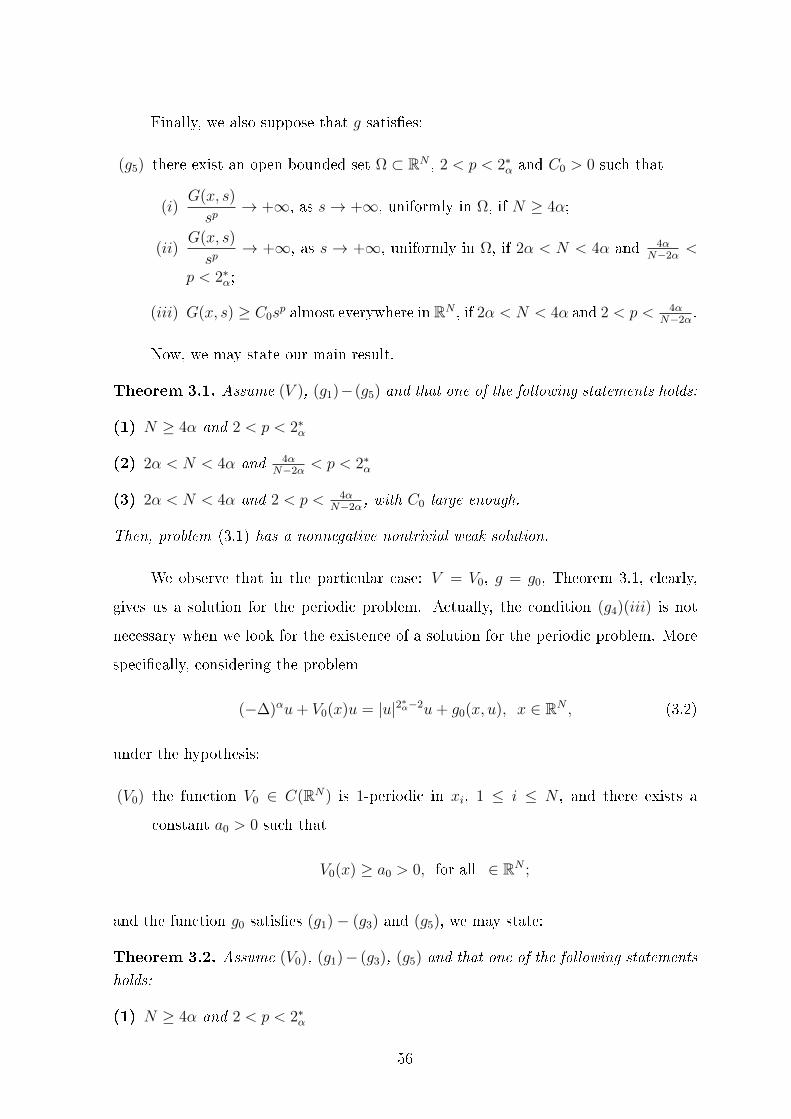
Finally, we also suppose that g satises:

(g5) there exist an open bounded set Ω ⊂ RN , 2 < p < 2∗α and C0 > 0 such that

(i)G(x, s)

sp→ +∞, as s→ +∞, uniformly in Ω, if N ≥ 4α;

(ii)G(x, s)

sp→ +∞, as s → +∞, uniformly in Ω, if 2α < N < 4α and 4α

N−2α<

p < 2∗α;

(iii) G(x, s) ≥ C0sp almost everywhere in RN , if 2α < N < 4α and 2 < p < 4α

N−2α.

Now, we may state our main result.

Theorem 3.1. Assume (V ), (g1)−(g5) and that one of the following statements holds:

(1) N ≥ 4α and 2 < p < 2∗α

(2) 2α < N < 4α and 4αN−2α

< p < 2∗α

(3) 2α < N < 4α and 2 < p < 4αN−2α

, with C0 large enough.


We observe that in the particular case: V = V0, g = g0, Theorem 3.1, clearly,

gives us a solution for the periodic problem. Actually, the condition (g4)(iii) is not

necessary when we look for the existence of a solution for the periodic problem. More

specically, considering the problem

(−∆)αu+ V0(x)u = |u|2∗α−2u+ g0(x, u), x ∈ RN , (3.2)

under the hypothesis:

(V0) the function V0 ∈ C(RN) is 1-periodic in xi, 1 ≤ i ≤ N , and there exists a

constant a0 > 0 such that

V0(x) ≥ a0 > 0, for all ∈ RN ;

and the function g0 satises (g1)− (g3) and (g5), we may state:

Theorem 3.2. Assume (V0), (g1)− (g3), (g5) and that one of the following statements

holds:

(1) N ≥ 4α and 2 < p < 2∗α

56

(2) 2α < N < 4α and 4αN−2α

< p < 2∗α

(3) 2α < N < 4α and 2 < p < 4αN−2α

, with C0 large enough.


The (AR) condition has appeared in most of the studies for superlinear problems

and plays an important role in studying the existence of nontrivial solutions of many

nonlinear elliptic problems. Since Ambrosetti and Rabinowitz proposed the Mountain

Pass Theorem in their celebrated paper [2], the critical point theory has become one

of the main tools for nding solutions to elliptic equations of variational type. In

the subcritical case, the (AR) condition ensures that the EulerLagrange functional

associated with a (3.1)- type problem has a mountain pass geometry and also guarantees

the boundedness of the PalaisSmale sequence, so we can get the nontrivial solution

by using suitable versions of the Mountain Pass Theorem.

On the other hand, there are many cases where the nonlinear term does not

satisfy the (AR) condition (see Remark 3.3). Thus it becomes interesting to know if

a nontrivial solution exists in such situations. When α = 1, conditions weaker than

(AR) were used rst in [12, 27, 36]. In the case 0 < α < 1, we would like to mention

two works, one by Chang and Wang [10] and a paper by J. M. do Ó et al. [21].

Motivated by the above mentioned papers and by Lins and Silva [33], we study the

existence of a nontrivial solution to problem (3.1) where the subcritical perturbation

g(x, u) does not satisfy the (AR) condition. Moreover, we assume that the potential

V (x) and g(x, u) are asymptotically periodic at innity in x. In this sense our results

complement the study made in [10,21,43]. Moreover, we also complement [10,11,18,41]

in the sense that the potential V (x) belongs to a dierent class from those treated by

them.

Remark 3.3. An example of potential V (x) satisfying the hypothesis (V ) is given by

V (x) = e−1/(|x|+1), where a0 = e−1 and V0 ≡ 1, and if α = 1/2 and N = 2, an example

of nonlinearity g(x, s), satisfying the hypotheses (g1)− (g5), is given by

g(x, s) =

(

1 +1

|x|+ 1

)g0(x, s), if s > 0,

0, if s ≤ 0,

57

where g0 : R2 × R→ [0,+∞) is dened by

g0(x, s) =

%1(x)s ln (s+ 1) + %2(x)s2, if (x, s) ∈ R2 × [0,+∞),

0, if (x, s) ∈ R2 × (−∞, 0),

where %i : R2 → [0, 2] is a continuous function, %i 6= 0, 1-periodic in xi, with i ∈ 1, 2.Moreover, we consider that supp(%1) ∩ supp(%2) = ∅ and that B1 ⊂ supp(%2). Note

that g does not satisfy the (AR) condition (see details in Appendix A).

The outline of this chapter is as follows: In Section 2, we present some notations

and denitions about the fractional Laplacian operator, and we introduce the varia-

tional framework associated to Problems (3.1) and (3.2). In Section 3, we present some

auxiliary results which are used in the proofs of our results, we verify the geometric

conditions of the Mountain Pass Theorem and we present some results concerning the

behavior of the Cerami sequences. In Section 4 we study the minimax level. In Section

5 we prove some convergence results and, nally, in Section 6 and Section 7, we prove

Theorems 3.2 and 3.1.

Notations, denitions and variational setting

As seen in the introduction the operator (−∆)α can be represented [17, Lemma

3.2] as

(−∆)αu(x) = −1

2C(N,α)

∫RN

u(x+ z) + u(x− z)− 2u(x)

|z|N+2αdz, (3.3)

where

C(N,α) =

∫RN

1− cos(ζ1)

|ζ|N+2αdζ

−1

, ζ = (ζ1, ζ2, · · ·, ζN).

However, there is another way to dene this operator. In fact, when α = 1/2

there is an explicit form of calculating the half-Laplacian acting on a function u in the

whole space RN , as the normal derivative on the boundary of its harmonic extension

to the upper half-space RN+1+ = (x, y) ∈ RN+1 : y > 0, the so-called Dirichlet to

Neumann operator. The α derivative (−∆)α can be characterized in a similar way,

dening the α−harmonic extension to the upper half-space, see [9] and (3.5)-(3.6) for

details. This extension is commonly used in the recent literature since it allows to write

58

nonlocal problems in a local way and this permits to use the variational techniques for

these kind of problems. In particular, for nonlocal case in bounded domain, we would

like to mention two works, one by Barrios et al. [3], and a paper by Brandle et al. [6].

In order to prove our results, we consider the spaces Hα(RN) and X2α(RN+1+ )

dened as the completion of C∞0 (RN) and C∞0 (RN+1+ ), respectively, under the norms

‖u‖2Hα :=

∫RN

|2πξ|2α|u(ξ)|2dξ =

∫RN

|(−∆)α/2u|2dx,

‖w‖2X2α :=

∫RN+1+

κα y1−2α|∇w|2dxdy,

where κα = 21−2αΓ(1− α)/Γ(α).

The extension operator E2α : Hα(RN) → X2α(RN+1+ ) is well dened (see [6,

Lemmas 2.2 and 2.3]). For φ ∈ X2α(RN+1+ ), let us denote its trace on RN ×y = 0 as

φ(x, 0). This trace operator is also well dened and it was proved in [6, Lemmas 2.2

and 2.3] that

‖φ(·, 0)‖Hα(RN ) ≤ κ−1/2α ‖φ‖X2α(RN+1

+ ). (3.4)

For u ∈ Hα(RN), we say that w = E2α(u) is the α−harmonic extension of u to

the upper half-space, RN+1+ , if w is a solution to the problem −div(y1−2α∇w) = 0 in RN+1

+ ,

w = u in RN × 0.(3.5)

In [9] it is proved that

limy→0+

y1−2αwy(x, y) = − 1

κα(−∆)αu(x). (3.6)

As we pointed out at the beginning of this section, identity (3.6) allows to formu-

late nonlocal problems involving the fractional powers of the Laplacian in RN as local

problems in divergence form in the half-space RN+1+ . Motivated by (3.5) and (3.6), we

will consider the problem −div(y1−2α∇w) = 0 in RN+1+ ,

−κα∂w

∂ν= −V (x)u+ |u|2∗α−2u+ g(x, u) in RN × 0,

(3.7)

where∂w

∂ν= lim

y→0+y1−2αwy(x, y).

59

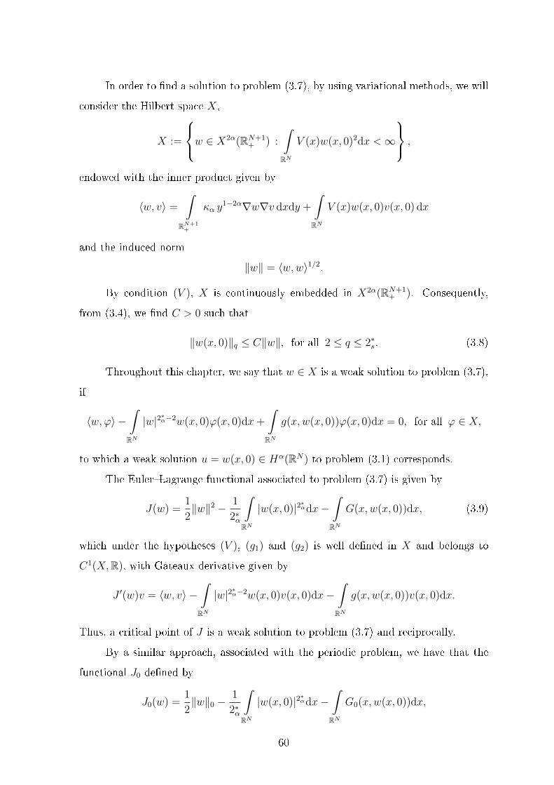
In order to nd a solution to problem (3.7), by using variational methods, we will

consider the Hilbert space X,

X :=

w ∈ X2α(RN+1+ ) :

∫RN

V (x)w(x, 0)2dx <∞

,

endowed with the inner product given by

〈w, v〉 =

∫RN+1+

κα y1−2α∇w∇v dxdy +

∫RN

V (x)w(x, 0)v(x, 0) dx

and the induced norm

‖w‖ = 〈w,w〉1/2.

By condition (V ), X is continuously embedded in X2α(RN+1+ ). Consequently,

from (3.4), we nd C > 0 such that

‖w(x, 0)‖q ≤ C‖w‖, for all 2 ≤ q ≤ 2∗s. (3.8)

Throughout this chapter, we say that w ∈ X is a weak solution to problem (3.7),

if

〈w,ϕ〉 −∫RN

|w|2∗α−2w(x, 0)ϕ(x, 0)dx+

∫RN

g(x,w(x, 0))ϕ(x, 0)dx = 0, for all ϕ ∈ X,

to which a weak solution u = w(x, 0) ∈ Hα(RN) to problem (3.1) corresponds.

The EulerLagrange functional associated to problem (3.7) is given by

J(w) =1

2‖w‖2 − 1

2∗α

∫RN

|w(x, 0)|2∗αdx−∫RN

G(x,w(x, 0))dx, (3.9)

which under the hypotheses (V ), (g1) and (g2) is well dened in X and belongs to

C1(X,R), with Gâteaux derivative given by

J ′(w)v = 〈w, v〉 −∫RN

|w|2∗α−2w(x, 0)v(x, 0)dx−∫RN

g(x,w(x, 0))v(x, 0)dx.

Thus, a critical point of J is a weak solution to problem (3.7) and reciprocally.

By a similar approach, associated with the periodic problem, we have that the

functional J0 dened by

J0(w) =1

2‖w‖0 −

1

2∗α

∫RN

|w(x, 0)|2∗αdx−∫RN

G0(x,w(x, 0))dx,

60

belongs to C1(X0,R), where

X0 =

w ∈ X2α(RN+1+ ) :

∫RN

V0(x)w(x, 0)2dx <∞

.

Since we are interested in nonnegative solutions, we consider

f(x, s) =

|s|2∗α−2s+ g(x, s) if s ≥ 0,

0 if s < 0,

throughout the remainder of this chapter.

Remark 3.4. Let w be a nonnegative weak solution to problem (3.7), to which a weak

solution u ∈ Hα(RN) to problem (3.1) corresponds. Then w = Eα(u) and w(x, 0) = u.

If w 6≡ 0, we have u 6= 0. Moreover, if u is suciently regular, we may ensure that

u > 0. In fact, if u(x0) = 0 for some x0 ∈ RN , then (−∆)αu(x0) = 0 and by the

representation formula (3.3), one obtains, at x0, that∫RN

u(x0 + z) + u(x0 − z)

|z|N+2αdz = 0,

yielding u = 0, a contradiction.

Preliminary results

In this section, we present two versions of the Mountain Pass Theorem which are

used in the proofs of Theorems 3.2 and 3.1. Furthermore, we verify the geometric con-

ditions of the Mountain Pass Theorem and we also present some results concerning the

behavior of the Cerami sequences of the associated functional: we show the bounded-

ness for the Cerami sequences and a proposition which will be essential to guarantee

that the solutions that we provide in our proofs of Theorems 3.2 and 3.1 are not trivial.

Versions of the Mountain Pass Theorem

As we observed in the introduction, the functional associated to problem (3.7)

does not satisfy the condition Palais-Smale. To overcome this diculty, we will use

two versions of the Mountain Pass Theorem which we will present below.

Let E be a real Banach space and I ∈ C1(E,R). We recall that I satises the

Cerami condition on level c, denoted by (Ce)c, if any sequence (un) ⊂ E for which

61

(i) I(un) → c and (ii) ‖I ′(un)‖E′(‖un‖E + 1) → 0, as n → ∞, possesses a convergent

subsequence. We say that (un) ⊂ E is a (Ce)c sequence if it satises (i)− (ii).

Theorem 3.5. Let E be a real Banach space. Suppose that I ∈ C1(E,R), I(0) = 0

and

(I1) there exist β, ρ > 0 such that I |∂Bρ(0)≥ β > 0,

(I2) there exists e ∈ E with ‖e‖ > ρ such that I(e) ≤ 0.

Then I possesses a (Ce)c sequence with c ≥ β > 0 given by

c = infγ∈Γ

maxt∈[0,1]

I(γ(t)),

where

Γ = γ ∈ C([0, 1], X) : γ(0) = 0 and γ(1) = e. (3.10)

We will also need to establish a local version of Theorem 3.5, which has been

proved in [33] (or [26, Theorem 7.10]). For this, we consider K the set of critical points

of I and given b ∈ R, we dene Kb = u ∈ X : u ∈ K and I(u) = b.

Theorem 3.6. Let E be a real Banach space. Suppose that I ∈ C1(E,R) satises

I(0) = 0, (I1) and (I2). If there exists γ0 ∈ Γ, Γ dened by (3.10), such that

c = maxt∈[0,1]

I(γ0(t)) > 0,

then I possesses a nontrivial critical point u ∈ Kc ∩ γ0([0, 1]).

Mountain pass geometry

The next lemma shows that the functional associated to problem (3.7) satises

the geometric properties of the Mountain Pass Theorem.

Lemma 3.7. Suppose that (V ), (g1) and (g2) are satised. Then the functional J ,

dened by (3.9), satises the conditions of Theorem 3.5.

Proof. Since G(x, 0) = 0 for all x ∈ RN , it follows that J(0) = 0. Thus we must show

that J satises the conditions (I1) and (I2). To verify (I1), note that by (g1) and (g2),

given any ε > 0, there exists Cε > 0 such that

|g(x, s)| ≤ ε|s|+ Cε|s|q1−1 for all (x, s) ∈ RN × R, (3.11)

|G(x, s)| ≤ ε

2|s|2 +

Cεq1

|s|q1 for all (x, s) ∈ RN × R. (3.12)

62

From (3.12),∫RN

|G(x,w(x, 0))| dx ≤ ε

2

∫RN

w(x, 0)2dx+Cεq1

∫RN

|w(x, 0)|q1dx, for all w ∈ X. (3.13)

By using the condition (V ) in (3.13), we obtain∫RN

G(x,w(x, 0))dx ≤ ε

2a0

∫RN

V (x)w(x, 0)2dx+Cεq1

∫RN

|w(x, 0)|q1dx. (3.14)

Combining (3.8) and (3.14), we can nd two positive constants, C1 and C2, such that

J(w) ≥(

1

2− ε

2a0

)ρ2 − C1ρ

2∗α − C2ρq1 if ‖w‖ = ρ.

Since q1, 2∗α > 2, choosing 0 < ε < a0, we conclude, for ρ suciently small, that

β := inf‖w‖=ρ

J > 0.

Hence (I1) holds. In order to verify the condition (I2), consider ϕ ∈ C∞0 (RN+1+ ,R+)

with ϕ(x, 0) 6≡ 0. From (g4)(i), G(x, tϕ) ≥ 0 for every t > 0. Thus,

J(tϕ) ≤ t2

2‖ϕ‖2 − t2

∗α

2∗α

∫RN

|ϕ(x, 0)|2∗αdx→ −∞, as t→ +∞.

Setting e0 = tu with t large enough, the condition (I2) is satised. This completes the

proof.

By Lemma 3.7 and Theorem 3.5, we have

Corollary 3.8. Suppose that (V ), (g1) and (g2) are satised. Then

cM = infγ∈Γ

maxt∈[0,1]

J(γ(t)) ≥ β > 0,

where Γ = γ ∈ C([0, 1], X) : γ(0) = 0 and γ(1) = e0, and the functional J possesses

a (Ce)cM sequence.

Behaviour of the Cerami sequences

Here we verify the boundedness of the (Ce)c sequences associated with the func-

tional J . Before stating the next lemma, we establish a simple result that will be

employed several times throughout this chapter. In the following lemma, given h ∈ F ,

we set Dε = x ∈ RN : |h(x)| ≥ ε and Dε(R) = x ∈ RN : |h(x)| ≥ ε and |x| ≥ R.

Lemma 3.9. Suppose that h ∈ F . Then |Dε(R)| → 0 as R→∞.

63

Proof. Since h ∈ F , |Dε| < ∞ for all ε > 0. Consequently, this Lemma is equivalent

to the following claim:

limn→∞

|Dε ∩ (RN \BRn)| = 0,

for every sequence (Rn) ⊂ R such that Rn →∞. Consider the real function ξ : RN → Rgiven by

ξ(x) =

1 for x ∈ Dε,

0 for x ∈ RN \Dε.

Note that ‖ξ‖1 = |Dε|, then ξ ∈ L1(RN). Dening the sequence of functions ξn : RN →R by

ξn(x) =

1 for x ∈ Dε ∩ (RN \BRn),

0 for x ∈ RN \Dε ∩ (RN \BRn),

it follows that |ξn(x)| ≤ |ξ(x)| and ξn(x) → 0 almost everywhere in RN as n → ∞.

Consequently, by the dominated convergence theorem,

|Dε ∩ (RN \BRn)| = ‖ξn‖1 → 0 as n→ +∞.

This completes the proof of Lemma 3.9.

Lemma 3.10. Suppose that (V ), (g1) − (g3) are satised and let (vn) ⊂ X be an

arbitrary Cerami sequence of J on level c, that is,

J(vn) = c+ on(1) and ‖J ′(vn)‖∗(1 + ‖vn‖) = on(1). (3.15)

Then (vn) is bounded in X.

Proof. We must show that there exists M > 0 such that

‖vn‖2 =

∫RN+1+

κα y1−2α|∇vn|2dxdy +

∫RN

V (x)vn(x, 0)2dx ≤M.

By the rst condition in (3.15), (3.12) and (V ), we have

1

2‖vn‖2 ≤

1

2∗α

∫RN

|vn(x, 0)|2∗αdx+

ε

2a0

∫RN

V (x)|vn(x, 0)|2dx+Cεq1

∫RN

|vn(x, 0)|q1dx+ c+ on(1).

Given 0 < δ ≤ 1 to be chosen later, there exists 0 < δ1 < 1 such that |s|q1 ≤ δ|s|2 forall |s| ≤ δ1. Then, by using (V ), it follows that

1

2

∫RN+1

+


(1

2− ε

2a0

) ∫RN

V (x)|vn(x, 0)|2dx

≤ 1

2∗α

∫RN

|vn(x, 0)|2∗αdx+

Cεq1

∫|vn(x,0)|≤δ1

|vn(x, 0)|q1dx+Cεq1

∫|vn(x,0)|>δ1

|vn(x, 0)|q1dx+ c+ on(1)

≤ 1

2∗α

∫RN

|vn(x, 0)|2∗αdx+

Cεδ

q1a0

∫RN

V (x)|vn(x, 0)|2dx+Cεq1

∫|vn(x,0)|>δ1

|vn(x, 0)|q1dx+ c+ on(1),

64

which yields

1

2

∫RN+1+


(1

2− ε

2a0

− Cεδ

q1a0

) ∫RN

V (x)|vn(x, 0)|2dx

≤ 1

2∗α

∫RN

|vn(x, 0)|2∗αdx+Cεq1

∫|vn(x,0)|>δ1

|vn(x, 0)|q1dx+ c+ on(1).

Note that if |s| > δ1, there exists C1 > 0 such that |s|q1 ≤ C1|s|2∗α . Thus,

1

2

∫RN+1+


(1

2− ε

2a0

− Cεδ

q1a0

) ∫RN

V (x)|vn(x, 0)|2dx

≤(

1

2∗α+CεC1

q1

) ∫RN

|vn(x, 0)|2∗αdx+ c+ on(1).

(3.16)

Taking δ and ε suciently small such that 12− ε

2a0− δCε

q1a0> 0. Hence, in order to

conclude the proof of the lemma, it suces to show that the right hand side in (3.16)

is bounded. Note that without loss of generality we may assume that∫RN

|vn(x, 0)|2∗αdx ≥ c. (3.17)

To prove that ‖vn(x, 0)‖2∗α is bounded, we begin with the estimate

J(vn)−1

2J ′(vn)vn =

(1

2− 1

2∗α

) ∫RN

|vn(x, 0)|2∗αdx+

∫RN

[1

2g(x, vn(x, 0))vn(x, 0)−G(x, vn(x, 0)

]dx,

which by (g3), implies

J(vn)− 1

2J ′(vn)vn ≥

α

N

∫RN

|vn(x, 0)|2∗αdx−∫RN

h1(x)dx−∫RN

h2(x)|vn(x, 0)|q2dx. (3.18)

Combining (3.15), (3.18) and the fact that h1 ∈ L1(RN), we can nd a constant C > 0

such thatα

N

∫RN

|vn(x, 0)|2∗αdx ≤∫RN

h2(x)|vn(x, 0)|q2dx+ C. (3.19)

Given ε > 0, we set Dε(R) = x ∈ RN : |h2(x)| ≥ ε and |x| ≥ R for all R > 0. Then,since h2 ∈ F , applying Lemma 3.9, there exists R = Rε > 0 such that |Dε(R)| < ε. ByHölder's inequality,

∫Dε(R)

h2(x)|vn(x, 0)|q2dx ≤ ‖h2‖∞

∫Dε(R)

12∗α

2∗α−q2 dx

2∗α−q2

2∗α ∫Dε(R)

|vn(x, 0)|2∗αdx

q22∗α

≤ ‖h2‖∞ε2∗α−q2

2∗α

∫Dε(R)

|vn(x, 0)|2∗αdx

q22∗α

.

(3.20)

65

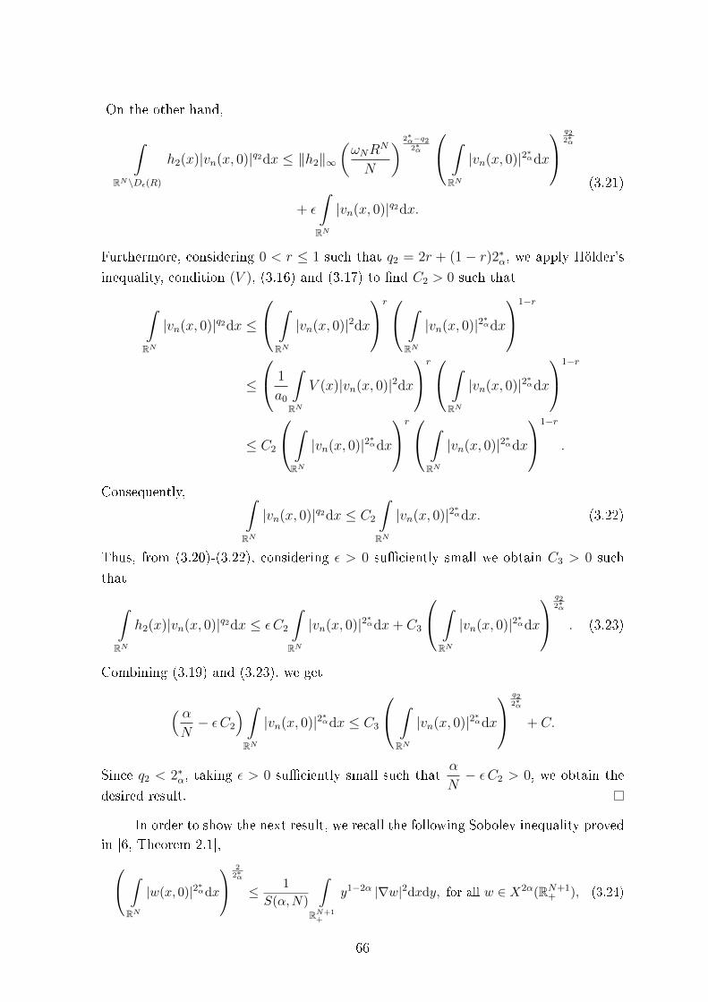
On the other hand,

∫RN\Dε(R)

h2(x)|vn(x, 0)|q2dx ≤ ‖h2‖∞(ωNR

N

N

) 2∗α−q22∗α

∫RN

|vn(x, 0)|2∗αdx

q22∗α

+ ε

∫RN

|vn(x, 0)|q2dx.

(3.21)

Furthermore, considering 0 < r ≤ 1 such that q2 = 2r + (1 − r)2∗α, we apply Hölder's

inequality, condition (V ), (3.16) and (3.17) to nd C2 > 0 such that

∫RN

|vn(x, 0)|q2dx ≤

∫RN

|vn(x, 0)|2dx

r ∫RN

|vn(x, 0)|2∗αdx

1−r

≤

1

a0

∫RN

V (x)|vn(x, 0)|2dx

r ∫RN

|vn(x, 0)|2∗αdx

1−r

≤ C2

∫RN

|vn(x, 0)|2∗αdx

r ∫RN

|vn(x, 0)|2∗αdx

1−r

.

Consequently, ∫RN

|vn(x, 0)|q2dx ≤ C2

∫RN

|vn(x, 0)|2∗αdx. (3.22)

Thus, from (3.20)-(3.22), considering ε > 0 suciently small we obtain C3 > 0 such

that

∫RN

h2(x)|vn(x, 0)|q2dx ≤ ε C2

∫RN

|vn(x, 0)|2∗αdx+ C3

∫RN

|vn(x, 0)|2∗αdx

q22∗α

. (3.23)

Combining (3.19) and (3.23), we get

( αN− ε C2

) ∫RN

|vn(x, 0)|2∗αdx ≤ C3

∫RN

|vn(x, 0)|2∗αdx

q22∗α

+ C.

Since q2 < 2∗α, taking ε > 0 suciently small such thatα

N− ε C2 > 0, we obtain the

desired result.

In order to show the next result, we recall the following Sobolev inequality provedin [6, Theorem 2.1], ∫

RN

|w(x, 0)|2∗αdx

22∗α

≤ 1

S(α,N)

∫RN+1+

y1−2α |∇w|2dxdy, for all w ∈ X2α(RN+1+ ), (3.24)

66

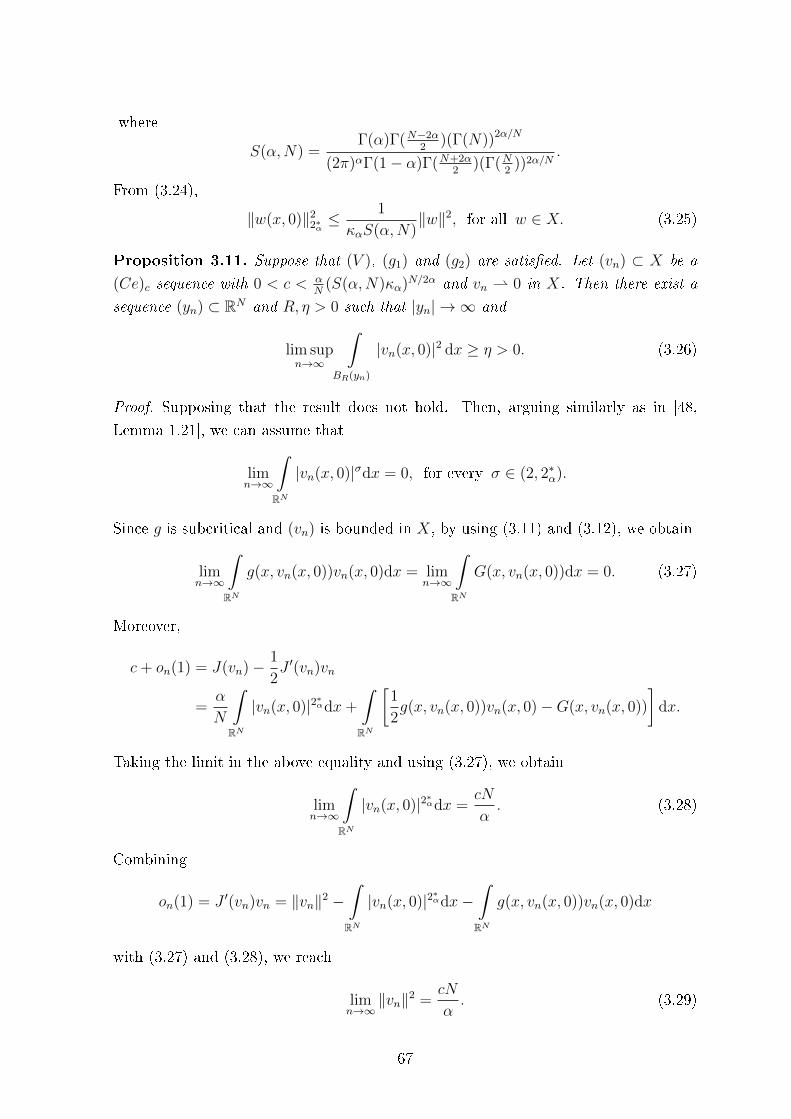
where

S(α,N) =Γ(α)Γ(N−2α

2)(Γ(N))2α/N

(2π)αΓ(1− α)Γ(N+2α2

)(Γ(N2

))2α/N.

From (3.24),

‖w(x, 0)‖22∗α≤ 1

καS(α,N)‖w‖2, for all w ∈ X. (3.25)

Proposition 3.11. Suppose that (V ), (g1) and (g2) are satised. Let (vn) ⊂ X be a

(Ce)c sequence with 0 < c < αN

(S(α,N)κα)N/2α and vn 0 in X. Then there exist a

sequence (yn) ⊂ RN and R, η > 0 such that |yn| → ∞ and

lim supn→∞

∫BR(yn)

|vn(x, 0)|2 dx ≥ η > 0. (3.26)

Proof. Supposing that the result does not hold. Then, arguing similarly as in [48,

Lemma 1.21], we can assume that

limn→∞

∫RN

|vn(x, 0)|σdx = 0, for every σ ∈ (2, 2∗α).

Since g is subcritical and (vn) is bounded in X, by using (3.11) and (3.12), we obtain

limn→∞

∫RN

g(x, vn(x, 0))vn(x, 0)dx = limn→∞

∫RN

G(x, vn(x, 0))dx = 0. (3.27)

Moreover,

c+ on(1) = J(vn)− 1

2J ′(vn)vn

=α

N

∫RN

|vn(x, 0)|2∗αdx+

∫RN

[1

2g(x, vn(x, 0))vn(x, 0)−G(x, vn(x, 0))

]dx.

Taking the limit in the above equality and using (3.27), we obtain

limn→∞

∫RN

|vn(x, 0)|2∗αdx =cN

α. (3.28)

Combining

on(1) = J ′(vn)vn = ‖vn‖2 −∫RN

|vn(x, 0)|2∗αdx−∫RN

g(x, vn(x, 0))vn(x, 0)dx

with (3.27) and (3.28), we reach

limn→∞

‖vn‖2 =cN

α. (3.29)

67

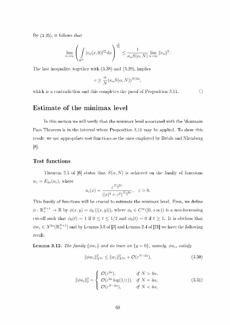
By (3.25), it follows that

limn→∞

∫RN

|vn(x, 0)|2∗αdx

22∗α

≤ 1

καS(α,N)limn→∞

‖vn‖2.

The last inequality, together with (3.28) and (3.29), implies

c ≥ α

N(καS(α,N))N/2α,

which is a contradiction and this completes the proof of Proposition 3.11.

Estimate of the minimax level

In this section we will verify that the minimax level associated with the Mountain

Pass Theorem is in the interval where Proposition 3.11 may be applied. To show this

result, we use appropriate test functions as the ones employed by Brézis and Nirenberg

[8].

Test functions

Theorem 2.1 of [6] states that S(α,N) is achieved on the family of functions

wε = E2α(uε), where

uε(x) =εN−2α

2

(|x|2 + ε2)N−2α

2

, ε > 0.

This family of functions will be crucial to estimate the minimax level. First, we dene

φ : RN+1+ → R by φ(x, y) = φ0 (|(x, y)|), where φ0 ∈ C∞([0,+∞)) is a non-increasing

cut-o such that φ0(t) = 1 if 0 ≤ t ≤ 1/2 and φ0(t) = 0 if t ≥ 1. It is obvious that

φwε ∈ X2α(RN+1+ ) and by Lemma 3.8 of [3] and Lemma 2.4 of [21] we have the following

result:

Lemma 3.12. The family φwε and its trace on y = 0, namely, φuε, satisfy

‖φwε‖2X2α ≤ ‖wε‖2

X2α +O(εN−2α), (3.30)

‖φuε‖22 =

O(ε2α), if N > 4α,

O(ε2α log(1/ε)), if N = 4α,

O(εN−2α), if N < 4α,

(3.31)

68

for ε > 0 suciently small. Dene

ηε =φwε‖φuε‖2∗α

,

then

‖ηε‖2X2α ≤ καS(α,N) +O(εN−2α), (3.32)

‖ηε(x, 0)‖22 =

O(ε2α), if N > 4α,

O(ε2α log(1/ε)), if N = 4α,

O(εN−2α), if N < 4α,

(3.33)

and

‖ηε(x, 0)‖qq =

O(ε

2N−(N−2α)q2 ), if q ≥ N

N−2α,

O(ε(N−2α)q

2 ), if q ≤ NN−2α

.(3.34)

As a rst consequence of Lemma 3.12, we obtain the following result.

Lemma 3.13. Suppose that (V ), (g1), (g2) and (g4)(i) are satised. Consider tε > 0

such that

J(tεηε) = maxJ(tηε) : t > 0.

Then, there exist ε0 > 0 and positive constants T and T such that T ≤ tε ≤ T for

every 0 < ε < ε0.

Proof. In view of Lemma 3.7, (g4)(i) and the denition ηε, there exists a positive

constant β such that

β ≤ J(tεηε) ≤t2ε2‖ηε‖2 − t

2∗αε

2∗α

∫RN

η2∗αε (x, 0)dx =

t2ε2‖ηε‖2 − t

2∗αε

2∗α,

which implies that

β ≤ t2ε2‖ηε‖2 and

t2∗αε

2∗α≤ t2ε

2‖ηε‖2 − β. (3.35)

From (3.32) and (3.33), we obtain a positive constant C such that ‖ηε‖ ≤ C for ε > 0

suciently small. By using (3.35), there exist positive constants T and T such that

T ≤ tε ≤ T . This completes the proof.

Now we are ready to prove the main result of this section.

Proposition 3.14. Suppose that (V ), (g1), (g2), (g4) are satised. Furthermore, we

assume one of the following conditions

(g5)(i) if N ≥ 4α.

(g5)(ii) if 2α < N < 4α and4α

N − 2α< p < 2∗α.

69

(g5)(iii) if 2α < N < 4α and 2 < p <4α

N − 2α.

Then there exists v ∈ X \ 0 such that

maxt≥0

J(tv) <α

N(S(α,N)κα)N/2α. (3.36)

Proof. Consider tε as dened by Lemma 3.13, it is clear that

J(tεηε) =t2ε2‖ηε‖2 − t

2∗αε

2∗α−∫RN

G(x, tεηε(x, 0))dx.

Considering the function hε : [0,∞) → R given by hε(t) = 12‖ηε‖2t2 − 1

2∗αt2∗α , we have

that tε,0 = ‖ηε‖2/(2∗α−2) is a maximum point of hε and hε(tε,0) = αN‖ηε‖N/α. This,

together with (3.32), implies

J(tεηε) ≤α

N(‖ηε‖2)N/2α −

∫RN

G(x, tεηε(x, 0))dx

≤ α

N

(καS(α,N) +O(εN−2α) + ‖V ‖∞‖ηε‖2

2

)N/2α − ∫RN


Consequently, by using (3.33) we reach

J(tεηε) ≤

α

N(καS(α,N))

N/2α+O

(ε2α)−∫RN

G(x, tεηε(x, 0))dx, if N > 4α,

α

N(καS(α,N))

N/2α+O

(ε2α log(1/ε)

)−∫RN

G(x, tεηε(x, 0))dx, if N = 4α,

α

N(καS(α,N))

N/2α+O(εN−2α)−

∫RN

G(x, tεηε(x, 0))dx, if N < 4α.

(3.37)

Indeed, if N > 4α,

J(tεηε) ≤α

N

(καS(α,N) +O(εN−2α) +O(ε2α)

)N/2α − ∫RN


=α

N

(καS(α,N) +O(ε2α)

)N/2α − ∫RN


Applying the inequality

(b+ c)σ ≤ bσ + σ(b+ c)σ−1c, with b, c ≥ 0, σ ≥ 1, (3.38)

we get

J(tεηε) ≤α

N(καS(α,N))N/2α +O

(ε2α)−∫RN


This proves the rst estimate of (3.37). For N = 4α, note that

J(tεηε) ≤α

N

(καS(α,N) +O(εN−2α) +O

(ε2α log(1/ε)

))N/2α − ∫RN


=α

N

(καS(α,N) +O

(ε2α log(1/ε)

))N/2α − ∫RN


70

Again by using (3.38), we get

J(tεηε) ≤α

N(καS(α,N))N/2α +O

(ε2α log(1/ε)

)−∫RN


This proves the second estimate of (3.37). For N < 4α, combining (3.33) and (3.38),

it is immediate that

J(tεηε) ≤α

N(καS(α,N))N/2α +O(εN−2α)−

∫RN


This completes the proof of (3.37).

Now consider

γ(ε) =

ε2α, if N > 4α,

ε2α log(1/ε), if N = 4α,

εN−2α, if N < 4α.

By using (3.37) we nd a positive constant Θ such that

J(tεηε) ≤α

N(καS(α,N))N/2α + γ(ε)

Θ− 1

γ(ε)

∫RN


. (3.39)

In order to prove Proposition 3.14, we just need to verify that

limε→0+

1

γ(ε)

∫RN

G(x, tεηε(x, 0))dx > Θ. (3.40)

Initially, observe that without loss of generality we may assume that B1 ⊂ Ω. On the

other hand, by (g5), given A > 0 there exists RA > 0 such that

G(x, s) ≥ Asp, for all (x, s) ∈ Ω× [RA,+∞). (3.41)

Moreover, by using Lemma 3.13 it is easy to see that there exists positive constant ν

such that

tεηε(x, 0) ≥ tεC1uε(x) ≥ TC1(2ε)−(N−2α)/2 ≥ νε−(N−2α)/2, for |x| < ε, (3.42)

with ε > 0 suciently small. It is clear that we may choose ε1 > 0 such that

νε−(N−2α)/2 ≥ RA, for 0 < ε < ε1. (3.43)

Combining (3.41), (3.42) and (3.43), we have

G(x, tεηε(x, 0)) ≥ Aνε−(N−2α)p/2, for |x| < ε.

Furthermore, by (g4)∫RN

G(x, tεηε(x, 0))dx ≥∫

Bε(0)

Aνε−(N−2α)p/2dx−∫

Ω\Bε(0)

(tεηε(x, 0))2dx,

71

which, together with Lemma 3.13, gives∫RN

G(x, tεηε(x, 0))dx ≥ AνωNε−(N−2α)p/2+N − T 2‖ηε‖2

2. (3.44)

Now, in order to verify (3.40), we should consider the following cases:

Case 1: N > 4α.

From (3.44) and (3.33), we obtain

1

γ(ε)

∫RN

G(x, tεηε(x, 0))dx ≥ AνωNε−(N−2α)p/2+(N−2α) −O (1) .

Since −(N − 2α)p/2 + (N − 2α) < 0, we have that for ε > 0 suciently small (3.40)

is satised.

Case 2: N = 4α.

From (3.44) and (3.33), we have

1

γ(ε)

∫RN

G(x, tεηε(x, 0))dx ≥ AνωNε−(N−2α)p/2+N

ε2α log(1/ε)−O (1) .

But,

limε→0+

ε−(N−2α)p/2+N

ε2α log(1/ε)= +∞.

Consequently, we get that (3.40) holds, for ε > 0 suciently small.

Case 3: 2α < N < 4α and 4αN−2α

< p < 2∗α.

Combining (3.44) and (3.33), we obtain

1

γ(ε)

∫RN

G(x, tεηε)dx ≥ AνωNε−(N−2α)p/2+2α −O(1).

Since −(N − 2α)p/2 + 2α < 0, we get that (3.40) holds, for ε > 0 suciently small.

Case 4: 2α < N < 4α and 2 < p <4α

N − 2α.

By (g5)(iii),

G(x, s) ≥ C0sp, for all (x, s) ∈ RN × [0,+∞), (3.45)

72

where C0 ' ετ with τ to be chosen later. Here, we need to consider two cases:

If 2 < p ≤ N/(N − 2α). By applying Lemma 3.13, (3.45) and (3.34), we get

1

γ(ε)

∫RN

G(x, tεηε)dx ≥ O(ε(N−2α)p/2−(N−2α)+τ ),

which implies that (3.40) holds, since τ < (N − 2α)(2− p)/2.

If N/(N − 2α) ≤ p < 4α/(N − 2α). By applying Lemma 3.13, (3.45) and (3.34), we

get1

γ(ε)

∫RN

G(x, tεηε)dx ≥ O(εN−(N−2α)p/2−(N−2α)+τ ),

which implies that (3.40) holds, since τ < (N − 2α)p/2 − 2α. This concludes the

proof.

Convergence results

In this section, we prove two lemmas which are required in later sections.

Lemma 3.15. Suppose that (V ) and (g4) are satised. Let (vn) ⊂ X be a bounded

sequence in X and wn(x, 0) = w(x−yn, 0), where w ∈ X and (yn) ⊂ RN . If |yn| → ∞,

then

[V0(x)− V (x)]vn(x, 0)wn(x, 0)→ 0,

[g0(x, vn(x, 0))− g(x, vn(x, 0))]vn(x, 0)wn(x, 0)→ 0,

in L1(RN), as n→∞.

Proof. Given δ > 0, since w(x, 0) ∈ Lq(RN) for all 2 ≤ q ≤ 2∗α, we nd 0 < ε < δ such

that, for each measurable set A ⊂ RN satisfying |A| < ε,∫A

|w(x, 0)|2dx < δ and∫A

|w(x, 0)|2∗α

2∗α−q3 dx < δ. (3.46)

The condition (V ) implies V0 − V ∈ F and by Lemma 3.9 there exists R1 > 0 such

that |Dε(R1)| < ε, where Dε(R1) = x ∈ RN : |V0(x) − V (x)| ≥ ε and |x| > R1.

73

Thus, applying Hölder's inequality and (V ), we obtain∫RN\BR1

|V0(x)− V (x)||vn(x, 0)||wn(x, 0)|dx

≤ ‖V0‖∞∫

Dε(R1)

|vn(x, 0)||wn(x, 0)|dx+ ε

∫Fε

|vn(x, 0)||wn(x, 0)|dx

≤ ‖V0‖∞

∫Dε(R1)

|vn(x, 0)|2dx

12 ∫Dε(R1)

|wn(x, 0)|2dx

12

+ ε

∫Fε

|vn(x, 0)|2dx

12∫Fε

|wn(x, 0)|2dx

12

,

where Fε := RN \ (BR1 ∪Dε(R1)). Consequently,∫RN\BR1

|V0(x)− V (x)||vn(x, 0)||wn(x, 0)|dx

≤ ‖V0‖∞‖vn(x, 0)‖2‖wn(x, 0)‖L2(Dε(R1)) + δ‖vn(x, 0)‖2‖w(x, 0)‖2.

Using (3.46) and the fact that (vn) is bounded in X, we obtain a constant C1 > 0 such

that ∫RN\BR1

|V0(x)− V (x)||vn(x, 0)||wn(x, 0)|dx ≤ C1(δ1/2 + δ). (3.47)

On the other hand, by Hölder's inequality, (V ) and the boundedness of (vn) in X, we

nd C2 > 0 such that∫BR1

|V0(x)− V (x)||vn(x, 0)||wn(x, 0)|dx

≤ ‖V0‖∞

∫BR1

|vn(x, 0)|2dx

12∫BR1

|wn(x, 0)|2dx

12

≤ ‖V0‖∞‖vn(x, 0)‖2

∫BR1

(−yn)

|w(x, 0)|2dx

12

≤ C2

∫BR1

(−yn)

|w(x, 0)|2dx

12

.

(3.48)

Then, since w(x, 0) ∈ L2(RN) and |yn| → ∞, there exists n0 ∈ N such that∫BR1

|V0(x)− V (x)||vn(x, 0)||wn(x, 0)|dx ≤ C2δ, for all n ≥ n0. (3.49)

74

The inequalities (3.47), (3.49) and the fact that δ > 0 can be chosen arbitrarily small

imply that

[V0(x)− V (x)]vn(x, 0)wn(x, 0)→ 0 in L1(RN), as n→∞.

This proves the rst convergence of the lemma. In order to verify the second limit, given

R2 > 0, we dene An = (RN \ BR2) ∩ x ∈ RN : |vn(x)| ≤ 1, Bn = RN \ (An ∪ BR2),

Dε(R2) = x ∈ RN : |h3(x)| ≥ ε and |x| ≥ R2 and we split∫RN

|g0(x, vn(x, 0))− g(x, vn(x, 0))||vn(x, 0)||wn(x, 0)|dx = I1,n + I2,n + I3,n,

where

I1,n :=

∫An

|g0(x, vn(x, 0))− g(x, vn(x, 0))||vn(x, 0)||wn(x, 0)|dx,

I2,n :=

∫Bn

|g0(x, vn(x, 0))− g(x, vn(x, 0))||vn(x, 0)||wn(x, 0)|dx,

I3,n :=

∫BR2

|g0(x, vn(x, 0))− g(x, vn(x, 0))||vn(x, 0)||wn(x, 0)|dx.

We will estimate each one of these integrals. For I1,n, note that by the condition

(g4)(ii),

I1,n ≤∫An

|h3(x)||vn(x, 0)|q3 |wn(x, 0)|dx =: I1,n.

By Lemma 3.9 and the fact that h3 ∈ F , we can nd R2 > 0 such that |Dε(R2)| < ε.

Then, by Hölder's inequality

I1,n ≤ ‖h3‖∞

∫An∩Dε(R2)

|vn(x, 0)|2∗αdx

q32∗α ∫An∩Dε(R2)

|wn(x, 0)|2∗α

2∗α−q3 dx

2∗α−q3

2∗α

+ ε

∫An\Dε(R2)

|vn(x, 0)|2∗αdx

q32∗α ∫An\Dε(R2)

|wn(x, 0)|2∗α

2∗α−q3 dx

2∗α−q3

2∗α

.

Consequently,

I1,n ≤ ‖h3‖∞‖vn(x, 0)‖q32∗α‖wn(x, 0)‖

L

2∗α(2∗α−q3) (Dε(R2))

+ δ ‖vn(x, 0)‖q32∗α‖w(x, 0)‖ 2∗α

2∗α−q3.

Again using (3.46) and the fact that (vn) is bounded in X, we obtain a constant C3 > 0

such that

I1,n ≤ C3(δ(2∗α−q3)/2∗α + δ). (3.50)

75

On the other hand, again using the condition (g4)(ii) and Hölder's inequality we have

I2,n ≤ ‖h3‖∞

∫Dε(R2)

|vn(x, 0)|2∗αdx

q32∗α ∫Dε(R2)

|wn(x, 0)|2∗α

2∗α−q3 dx

2∗α−q3

2∗α

+ε

∫Bn\Dε(R2)

|vn(x, 0)|2∗αdx

q32∗α ∫Bn\Dε(R2)

|wn(x, 0)|2∗α

2∗α−q3 dx

2∗α−q3

2∗α

.

Thus, by the boundedness of (vn) in X and (3.46), there exists C4 > 0 such that

I2,n ≤ C4δ2∗α−q3

2∗α . (3.51)

Similarly to (3.48), we obtain that

I3,n ≤ C5

∫BR2

(−yn)

|w(x, 0)|2∗α

2∗α−q3 dx

2∗α−q3

2∗α

,

for some constant C5 > 0. Therefore, since w(x, 0) ∈ L2∗α/(2∗α−q3)(RN) and |yn| → +∞,

it follows that there exists n0 ∈ N such that

I3,n ≤ C5δ, for all n ≥ n0. (3.52)

Finally, the inequalities (3.50)−(3.52) and the fact that δ > 0 can be chosen arbitrarily

small imply that

[g0(x, vn(x, 0))− g(x, vn(x, 0))]vn(x, 0)wn(x, 0)→ 0 in L1(RN), as n→∞.

This concludes the proof.

Lemma 3.16. Suppose that 2 ≤ q < 2∗α and h ∈ F . Let (vn) ⊂ X be a sequence such

that vn v in X. Then

h(x)|vn(x, 0)|q → h(x)|v(x, 0)|q in L1(RN), as n→∞.

Proof. Arguing by contradiction, we suppose that there is a subsequence, still denoted

by (vn) and ε > 0 such that∫RN

|h(x)| | |vn(x, 0)|q − |v(x, 0)|q|dx ≥ ε for all n ∈ N. (3.53)

Now we dene Dδ(R) = x ∈ RN : |h(x)| ≥ δ and |x| > R. Since h ∈ F , by Lemma

3.9 there exists R = Rδ > 0 such that |Dδ(R)| < δ. Consequently, since the sequence

(vn) is bounded in X, by using Hölder's inequality and (3.8), we get

∫Dδ(R)

|vn(x, 0)|qdx ≤

∫Dδ(R)

12∗α

2∗α−qdx

2∗α−q2∗α ∫Dδ(R)

|vn(x, 0)|2∗αdx

q2∗α

≤ Cδ(2∗α−q)/2∗α ,

76

for some constant C > 0, which implies that∫Dδ(R)

|h(x)| | |vn(x, 0)|q − |v(x, 0)|q|dx ≤ ‖h‖∞∫

Dδ(R)

(|vn(x, 0)|q + |v(x, 0)|q)dx ≤ C1δ(2∗α−q)/2

∗α , (3.54)

for some constant C1 > 0. Still by the denition of Dδ(R) and boundedness of (vn) inX, there exists C2 > 0 such that∫RN\(BR∪Dδ(R))

|h(x)| | |vn(x, 0)|q − |v(x, 0)|q|dx ≤ δ∫RN

(|vn(x, 0)|q + |v(x, 0)|q)dx ≤ C2δ. (3.55)

Using that vn v inX, (3.4) and (V ), up to a subsequence, we have vn(x, 0)→ v(x, 0)

in Lqloc(RN) for all 1 ≤ q < 2∗α. Consequently, up to a subsequence, we obtain that

vn(x, 0) → v(x, 0) almost everywhere in BR and also that there exists wq ∈ Lq(BR)

such that |vn(x, 0)| ≤ wq. Thus, it follows by the Dominated Convergence Theorem

that ∫BR

||vn(x, 0)|q − |v(x, 0)|q|dx→ 0, as n→∞.

Since h ∈ L∞(RN) there exists n0 ∈ N such that∫BR

|h(x)|||vn(x, 0)|q − |v(x, 0)|q|dx < δ, for all n ≥ n0. (3.56)

Combining (3.54)− (3.56), for n suciently large, we get∫RN

|h(x)|||vn(x, 0)|q − |v(x, 0)|q|dx ≤ C1δ(2∗α−q)/2∗α + C2δ + δ.

But δ can be chosen arbitrarily small and so the inequality above contradicts (3.53),

which completes the proof.


With the aid of the results of the previous sections the goal of this section is

to nd a nontrivial critical point of J . First, recall that by Corollary 3.8 there exists

(vn) ⊂ X such that

J(vn)→ cM and ‖J ′(vn)‖∗(1 + ‖vn‖)→ 0, as n→∞. (3.57)

By Lemma 3.10 we may assume that vn v in X. Note that v is a critical point of

J . Indeed, since vn v in X, from (3.4) and (V ), up to a subsequence, we have that

77

vn(x, 0) → v(x, 0) in Lqloc(RN) for all 1 ≤ q < 2∗α. Consequently, up to a subsequence,

combining the Dominated Convergence Theorem and (3.11), we obtain∫RN

g(x, vn(x, 0))ϕ(x, 0)dx→∫RN

g(x, v(x, 0))ϕ(x, 0)dx, as n→ +∞

and ∫RN

|vn(x, 0)|2∗α−1ϕ(x, 0)dx→∫RN

|v(x, 0)|2∗α−1ϕ(x, 0)dx, as n→ +∞,

for each ϕ ∈ C∞0 (RN+1+ ). These convergences, together with the fact that vn v in X

and (3.57), imply

J ′(v)ϕ = limn→+∞

J ′(vn)ϕ = 0, for all ϕ ∈ C∞0 (RN+1+ ).

By density this holds for every ϕ ∈ X. This concludes the assertion.

If v 6≡ 0, Theorem 3.1 is proved. Assuming that v ≡ 0, the existence of a

nontrivial point critical of J is more delicate and it will involve several steps. Initially,

when v ≡ 0 in view of Proposition 3.14 we have cM < αN

(καS(α,N))N/2α. Furthermore,

by Proposition 3.11 there are a sequence (yn) ⊂ RN and R, η > 0 such that |yn| → ∞,

as n→∞, and

lim supn→∞

∫BR(yn)

|vn(x, 0)|2dx ≥ η > 0. (3.58)

Without loss of generality we may assume that (yn) ⊂ ZN . Then, dening un(x, y) =

vn(x+ yn, y), by the periodicity of V0 we have that ‖un(·, ·)‖0 = ‖vn(·+ yn, ·)‖0. Since

(vn) is also bounded in X0, it follows that (un) is bounded in X0. Thus, passing to a

subsequence if necessary, there is u ∈ X0 such that un u in X0.

Step 1. u is nonzero.

Indeed, by (3.58), up to a subsequence,

η1/2 ≤ ‖un(·, 0)‖L2(BR) ≤ ‖(un − u)(·, 0)‖L2(BR) + ‖u(·, 0)‖L2(BR).

Thus, from the Rellich-Kondrachov Embedding Theorem, we conclude that u is nonzero.

78

Step 2. J ′0(un)ϕ→ J ′0(u)ϕ, as n→∞, for all ϕ ∈ C∞0 (RN+1+ ).

By the Dominated Convergence Theorem, it is easy to see that for ϕ ∈ C∞0 (RN+1+ ), up

to a subsequence,∫RN

|un(x, 0)|2∗α−2un(x, 0)ϕ(x, 0)dx→∫RN

|u(x, 0)|2∗α−2u(x, 0)ϕ(x, 0)dx, as n→ +∞.

(3.59)

We also claim that∫RN

g0(x, un(x, 0))ϕ(x, 0)dx→∫RN

g0(x, u(x, 0))ϕ(x, 0)dx, as n→ +∞. (3.60)

In order to prove (3.60), observe that

[g0(x, u(x, 0))− g0(x, un(x, 0))]ϕ(x, 0) = [g0(x, u(x, 0))− g(x, un(x, 0))]ϕ(x, 0)

+ [g(x, un(x, 0))− g0(x, un(x, 0))]ϕ(x, 0).(3.61)

Now, using that un u in X0, (3.4) and (V ), up to a subsequence, we have un(x, 0)→

u(x, 0) in Lqloc(RN) for all 1 ≤ q < 2∗α. Consequently, from (g1), (g2) and the Dominated

Convergence Theorem, up to a subsequence,∫RN

g(x, un(x, 0))ϕ(x, 0)dx→∫RN

g(x, u(x, 0))ϕ(x, 0)dx, as n→ +∞, (3.62)

and by (g4)(ii) and the Dominated Convergence Theorem, up to a subsequence,∫RN

[g(x, un(x, 0))− g0(x, un(x, 0))]ϕ(x, 0)dx→∫RN

[g(x, u(x, 0))− g0(x, u(x, 0))]ϕ(x, 0)dx, (3.63)

as n→ +∞. Thus, combining (3.61)-(3.63), we obtain (3.60).

Since un u in X0, from (3.59) and (3.60) we conclude Step 2.

Step 3. Given ϕ ∈ C∞0 (RN+1+ ), we have that J ′0(un)ϕ = J ′0(vn)ϕn, where ϕn(x, y) =

ϕ(x− yn, y) and n ∈ N.

79

First, observe that

J ′0(un)ϕ =

∫RN+1+

κα y1−2α∇vn(x+ yn, y)∇ϕ(x, y)dxdy

+

∫RN

V0(x)vn(x+ yn, 0)ϕ(x, 0)dx−∫RN

g0(x, vn(x+ yn, 0))ϕ(x, 0)dx

−∫RN

|vn(x+ yn, 0)|2∗α−1vn(x+ yn, 0)ϕ(x, 0)dx.

By applying the denition of ϕn(x, y) and the periodicity of V0 and g0, we obtain

J ′0(un)ϕ =

∫RN+1+

κα y1−2α∇vn(z, y)∇ϕn(z, y)dzdy

+

∫RN

V0(z)vn(z, 0)ϕn(z, 0)dz −∫RN

g0(z, vn(z, 0))ϕn(z, 0)dz

−∫RN

|vn(z, 0)|2∗α−1vn(z, 0)ϕn(z, 0)dz

= J ′0(vn)ϕn.

This concludes Step 3.

Step 4. u is a critical point of J0.

Initially, note that

|J ′0(vn)ϕn − J ′(vn)ϕn| ≤∫RN

|V0(z)− V (z)||vn(z, 0)||ϕn(z, 0)|dz

+

∫RN

|g(z, vn(z, 0))ϕn(z, 0)− g0(z, vn(z, 0))ϕn(z, 0)|dz.

Then, applying Lemma 3.15, we get that

|J ′0(vn)ϕn − J ′(vn)ϕn| → 0, as n→∞. (3.64)

By (3.57) and using that ‖ϕn‖0 = ‖ϕ‖0, for all n ∈ N, we have J ′(vn)ϕn → 0 as

n→ +∞. Hence, by (3.64), we obtain

J ′0(vn)ϕn → 0, as n→∞.

80

From Step 2 and Step 3, we obtain that u is a critical point of J0 as claimed.

Step 5. We claim that

lim infn→∞

∫RN

[1

2g(x, vn(x, 0))vn(x, 0)−G(x, vn(x, 0))

]dx

≥∫RN

[1

2g0(x, u(x, 0))u(x, 0)−G0(x, u(x, 0))

]dx. (3.65)

Since vn 0 in X, in view of Lemma 3.16,∫RN

hi(x)|vn(x, 0)|qidx→ 0, as n→∞, (3.66)

for i ∈ 1, 2, 3, hi ∈ F and 2 ≤ qi < 2∗α. Recall that by (g4)(ii)

|g(x, s)s− g0(x, s)s| ≤ h3(x)|s|q3 .

This together with (3.66) imply∫RN

[g(x, vn(x, 0))vn(x, 0)− g0(x, vn(x, 0))vn(x, 0)] dx→ 0, as n→∞. (3.67)

Similarly, ∫RN

[G(x, vn(x, 0))−G0(x, vn(x, 0))] dx→ 0, as n→∞. (3.68)

From (3.67) and (3.68), we reach

lim infn→∞

∫RN

[1

2g(x, vn(x, 0))vn(x, 0)−G(x, vn(x, 0))

]dx

= lim infn→∞

∫RN

[1

2g0(x, vn(x, 0))vn(x, 0)−G0(x, vn(x, 0))

]dx.

Consequently, by the periodicity of g0 and the denition of (vn), we obtain

lim infn→∞

∫RN

[1

2g(x, vn(x, 0))vn(x, 0)−G(x, vn(x, 0))

]dx

= lim infn→∞

∫RN

[1

2g0(x, un(x, 0))un(x, 0)−G0(x, un(x, 0))

]dx. (3.69)

81

Now, from (g3) and (g4), we have that for s ≥ 0,

1

2g0(x, s)s−G0(x, s) ≥

1

2[g0(x, s)− g(x, s)]s+

1

2g(x, s)s−G(x, s) + [G(x, s)−G0(x, s)]

≥ −h1(x)− h2(x)sq2 − 1

2h3(x)s

q3 .

Hence, since g0(x, s) = 0 if s < 0, by Fatou's Lemma, it follows that

lim infn→∞

∫RN

[1

2g0(x, un(x, 0))un(x, 0)−G0(x, un(x, 0)) + h1(x) + h2(x)|un(x, 0)|q2 +

1

2h3(x)|un(x, 0)|q3

]dx

≥∫RN

[1

2g0(x, u(x, 0))u(x, 0)−G0(x, u(x, 0)) + h1(x) + h2(x)|u(x, 0)|q2 +

1

2h3(x)|u(x, 0)|q3

]dx.

By using (3.66) and (3.69), we obtain (3.65).

Step 6. J0(u) ≤ cM .

In order to show this fact, note that

J(vn)−1

2J ′(vn)vn =

α

N

∫RN

|vn(x, 0)|2∗αdx+

∫RN

[1

2g(x, vn(x, 0))vn(x, 0)−G(x, vn(x, 0))

]dx. (3.70)

By using the denition of (un) and the Fatou's Lemma we have

lim infn→∞

∫RN

|vn(x, 0)|2∗αdx ≥∫RN

|u(x, 0)|2∗αdx. (3.71)

Combining (3.57), (3.65), (3.70), (3.71) and Step 3, we reach

cM ≥α

N

∫RN

|u(x, 0)|2∗αdx+

∫RN

[1

2g0(x, u(x, 0))u(x, 0)−G0(x, u(x, 0))

]dx

= J0(u)− 1

2J ′0(u)u = J0(u), (3.72)

where we have used the fact that u is a critical point of J0 (see Step 4). This completes

Step 6.

Step 7. There exists γ0 ∈ Γ such that

cM = maxt∈[0,1]

J(γ0(t)). (3.73)

Note that maxJ0(tu); t ≥ 0 is unique. Indeed, we suppose that exist t1 and t2 such

that t1u and t2u are maximum points of J0 with t2 > t1, without loss of generality. By

using the fact that t2u is a critical point of J0, we have

t22‖u‖20 =

∫RN

g0(x, t2u)t2udx+ t2∗s2

∫RN

|u|2∗sdx.

82

By using (g4)(iii), we have that

0 = t22

‖u‖20 −

∫RN

g0(x, t2u)t−12 udx− t2

∗s−2

2 ‖u‖2∗s2∗s

< t22

‖u‖20 −

∫RN

g0(x, t1u)t−11 udx− t2

∗s−2

1 ‖u‖2∗s2∗s

.

Multiplying the above inequality by t21 and using the fact that t1u is also a critical

point of J0 we obtain

0 < t22

t21‖u‖20 −

∫RN

g0(x, t1u)t1udx− t2∗s

1 ‖u‖2∗s2∗s

= t22

(t2∗s1 ‖u‖

2∗s2∗s− t2

∗s

1 ‖u‖2∗s2∗s

)= 0,

but this is a contradiction, thus the maxJ0(tu); t ≥ 0 is unique.

Using this fact combined with (V ), (g4)(i) and Step 6, we have

cM ≤ maxt≥0

J(tu) ≤ maxt≥0

J0(tu) = J0(u) ≤ cM .

This implies that there exists γ0 ∈ Γ such that (3.73) holds.

In view of Theorem 3.6, J possesses a nontrivial critical point v on level cM . This

concludes the proof of Theorem 3.1.


The proof of Theorem 3.2 follows the same arguments of Theorem 3.1. In fact,

since g0 satises (g1)− (g3), applying Corollary 3.8, we nd a sequence (vn) ⊂ X0 such

that

J0(vn)→ cM and ‖J ′0(vn)‖∗(1 + ‖vn‖0)→ 0, as n→∞.

By Lemma 3.10, we may suppose, without loss of generality, that vn v0 in X0. From

(3.11) for g0, by using the same arguments as in the proof of Theorem 3.1, we have

that v0 is a critical point of J0. Hence, in order to prove Theorem 3.2 it suces to

assume that v0 ≡ 0.

In view of Proposition 3.14, it follows that cM < αN

(καS(α,N))N/2α. Furthermore,

by Proposition 3.11 there are a sequence (yn) ⊂ RN and R, η > 0 such that |yn| → ∞,

83

as n→∞, and

lim supn→∞

∫BR(yn)

|vn(x, 0)|2dx ≥ η > 0. (3.74)

As in the proof of Theorem 3.1, we may assume that (yn) ⊂ ZN . Then, dening

un(·, ∗) = vn(· + yn, ∗), n ∈ N, by the periodicity of V0 we have that ‖un(·, ∗)‖0 =

‖vn(· + yn, ∗)‖0 for all n ∈ N. Consequently, passing to a subsequence, if necessary,

there exists u0 ∈ X0 such that un u0 in X0. Similar to Step 4 we have that u0 is a

critical point of J0. Furthermore, (3.74) implies that u0 6≡ 0. This completes the proof

of Theorem 3.2.

84

Appendix A

Auxiliary results

Fractional Sobolev spaces and the fractional Laplacian

operator

In this section we present the suitable environment for the study of the nonlocal

equations: Fractional Sobolev spaces.

Considering 0 < α < 1 we may dene the fractional Sobolev space Wα,p(RN) for

any p ∈ [1,+∞) as follows

Wα,p(RN) :=

u ∈ Lp(RN);

|u(x)− u(y)||x− y|

Np

+α∈ Lp(RN × RN)

,

endowed with the natural norm

‖u‖α,p :=

∫RN

|u|pdx+

∫RN

∫RN

|u(x)− u(y)|p

|x− y|N+αpdxdy

1/p

,

where the term

[u]α,p :=

∫RN

∫RN

|u(x)− u(y)|p

|x− y|N+αpdxdy

1/p

is the so-called Gagliardo (semi)norm of u, see details in [17].

As in the classic case when α is an integer, any function in the fractional Sobolev

spaceWα,p(RN) can be approximated by a sequence of smooth functions with compact

support, it is what guarantees us the following result:

85

Theorem A.1. [17, Theorem 2.4] For any α > 0, the space C∞0 (RN) of smooth func-

tions with compact support is dense in Wα,p(RN).

When p = 2 we have an important case since Wα,2(RN) turn out to be Hilbert

space usually denoted by Hα(RN), which is strictly related to the fractional Laplacian

operator (−∆)α.

This nonlocal operator (−∆)α in RN is dened on the Schwartz class through the

Fourier transform,

((−∆)αu)(ξ) = |2πξ|2αu(ξ),

where u denotes the Fourier Transform of u, that is,

u(ξ) =

∫RN

e−2πix·ξu(x) dx.

The operator (−∆)α can be equivalently represented as

(−∆)αu(x) = C(N,α) limε→0+

∫Bcε (x)

u(x)− u(y)

|x− y|N+2αdy, (A.1)

where

C(N,α) =

∫RN

1− cos(ζ1)

|ζ|N+2αdζ

−1

, ζ = (ζ1, ζ2, · · ·, ζN).

E. Di Nezza et al. in [17] proved that we may write the singular integral in (A.1)

as a weighted second order dierential quotient.

Lemma A.2. [17, Lemma 3.2] Let 0 < α < 1 for any u on the Schwartz class,

(−∆)αu(x) = −1

2C(N,α)

∫RN

u(x+ y) + u(x− y)− 2u(x)

|y|N+2αdy, ∀x ∈ RN .

Moreover in [17] it has proved a relation between the fractional Laplacian operator

(−∆)α and the fractional Sobolev space Hα(RN) given by following result:

Lemma A.3. [17, Proposition 3.6] Let 0 < α < 1 and let u ∈ Hα(RN). Then,

[u]2α = 2C(N,α)−1‖(−∆)α2 u‖2

2.

Among some properties of these spaces we may mention the fractional Sobolev

inequalities. In this sense it is also important note that for N > αp the spaceWα,p(RN)

is continuously embedded in Lq(RN) for any q ∈ [p, p∗α] and in the limiting case N = αp

86

we have that Wα,p(RN) is continuously embedded in Lq(RN) for any q ∈ [p,∞). For a

proof of these results see [17, Theorems 6.5 and 6.9].

We conclude this section presenting an other approach for the fractional Laplacian

operator proposed by Caarelli and Silvestre in [9] which reduces the nonlocal operator

(−∆)α on functions dened in RN to a local operator on functions sitting in the higher

dimensional half-space RN+1+ , thus we have that

(−∆)αu(x) = κα limy→0+

(y1−2αwy(x, y)

),

where the function w : RN+1+ → R solves −div(y1−2α∇w) = 0 in RN+1

+ ,

w = u in RN × 0.

For more details see [9].

Variational formulation

In this section we present the variational formulation for the class of the problems

studied in Chapters 1 and 2. In order to do this, we consider the following class of

problems: (−∆)1/2u+ V (x)u = f(x, u) in R,

u ∈ H1/2(R) and u ≥ 0,(P )

and we denote X1 the space H1/2(R) endowed with the norm

‖u‖X1 =

1

2π

∫R2

|u(x)− u(y)|2

|x− y|2dx dy

+

∫R

V (x)u2 dx

1/2

.

Recall that u ∈ H1/2(R) is a weak solution to problem (P ) if

〈u, v〉 −∫R

f(x, u)vdx = 0, for all v ∈ H1/2(R). (A.2)

The purpose of this section is to prove that if u ∈ C∞(R) is suciently regular such that

(−∆)1/2u+ V (x)u = f(x, u) in R, then u satises (A.2) for every function v ∈ C∞0 (R)

such that∫RV (x)uvdx <∞ and

∫Rf(x, u)vdx <∞. Indeed, since

(−∆)1/2u(x) + V (x)u(x) = f(x, u) in R.

87

Multiplying both members of this equality by v and integrating, we obtain∫R

(−∆)1/2u(x)v(x)dx+

∫R

V (x)u(x)v(x)dx−∫R

f(x, u)v(x)dx = 0.

Now note that to obtain (A.2) it is sucient to show that∫R

(−∆)1/2u(x)v(x)dx+

∫R

V (x)u(x)v(x)dx = 〈u, v〉 . (A.3)

First, remember that

(−∆)1/2u(x) = − 1

2π

∫R

u(x+ y) + u(x− y)− 2u(x)

|y|2dy, for all x ∈ R.

Thus,∫R

(−∆)1/2u(x)v(x)dx =1

2π

∫R2

−v(x)(u(x+ y) + u(x− y)− 2u(x))

|y|2dydx.

Then, ∫R

(−∆)1/2u(x)v(x)dx =1

2π

∫R2

v(x)(u(x)− u(x+ y))

|y|2dydx

+1

2π

∫R2

v(x)(u(x)− u(x− y))

|y|2dydx.

By the change of variables formula we obtain

1

2π

∫R2

v(x)(u(x)− u(x+ y))

|y|2dydx =

1

2π

∫R2

v(θ)(u(θ)− u(ξ))

|ξ − θ|2dθdξ, (A.4)

and

1

2π

∫R2

v(x)(u(x)− u(x− y))

|y|2dydx =

1

2π

∫R2

v(ξ)(u(ξ)− u(θ))

|ξ − θ|2dθdξ. (A.5)

Combining (A.4) and (A.5), we get∫R

(−∆)1/2u(x)v(x)dx =1

2π

∫R2

(u(ξ)− u(θ)(v(ξ)− v(θ)

|ξ − θ|2dθdξ.

Thus, the equality (A.3) is valid and, therefore, (A.2) holds.

88

Dierentiability of the functional I

In this section we will study the properties of the functional I : X1 → R dened

by

I(u) =1

2‖u‖2

X1−∫R

F (x, u) dx,

where F (x, s) =

s∫0

f(x, t)dt. In order to show that the functional I ∈ C1(X1,R), we

need the following result.

Proposition A.4. Let (un) a sequence that converges strongly in H1/2(R). Then there

are a subsequence (unk) of (un) and v in H1/2(R) satisfying

|unk(x)| ≤ v(x), almost everywhere inR.

Proof. Let (un) be a strongly convergent sequence in H1/2(R), let us say, un → u in

H1/2(R). Hence (un) is Cauchy in H1/2(R). Thus, there is a subsequence (unk) of (un),

which, for simplicity, we denote by (uk) satisfying

‖uk+1 − uk‖1/2 ≤1

2k, for all k ∈ N. (A.6)

We dene

gn(x) =n∑k=1

|uk+1(x)− uk(x)| .

By the triangle inequality and by (A.6), it follows that

‖gn‖1/2 ≤n∑k=1

‖|uk+1 − uk|‖1/2 =n∑k=1

‖uk+1 − uk‖1/2 ≤n∑k=1

1

2k≤ 1.

Therefore, ‖gn‖1/2 ≤ 1. In particular,

[gn]1/2 ≤ 1 and ‖gn‖2 ≤ 1. (A.7)

Note that (gn) is a sequence of measurable functions that converges, let us say, to a

function g(x) =∑∞

k=1 |uk+1(x)− uk(x)|, almost everywhere in R. Then g is a measu-

rable function. From this we have that (g2n(x)) converges for g2(x) almost everywhere

in R. Moreover, we have that (gn) is a sequence of increasing functions and nonnega-

tive, then (g2n) is also increasing and nonnegative. Thus, by the monotone convergence

theorem

limn→∞

∫R

g2n(x)dx =

∫Rg2(x)dx. (A.8)

89

Let us show that g ∈ H1/2(R). First, note that g ∈ L2(R). Indeed, by (A.7) and (A.8)

we have that ∫R

g2(x)dx = limn→∞

∫R

g2n(x)dx ≤ 1.

Now, for x 6= y, we denote

hn(x, y) =(gn(x)− gn(y))2

|x− y|2.

Note that (hn) is a nonnegative functions sequence such that

hn(x, y)→ (g(x)− g(y))2

|x− y|2, almost everywhere inR2,

then, using Fatou's lemma and (A.7),∫R2

(g(x)− g(y))2

|x− y|2dxdy =

∫R2

lim infn→∞

(gn(x)− gn(y))2

|x− y|2dxdy

≤ lim infn→∞

∫R2

(gn(x)− gn(y))2

|x− y|2dxdy ≤ 1.

Therefore, g ∈ L2(R) and [g]1/2 ≤ 1, this is, g ∈ H1/2(R). Now, notice that for every

k ∈ N, we may write

g(x) =k−1∑i=1

|ui+1(x)− ui(x)|+k+j−1∑i=k

|ui+1(x)− ui(x)|+∞∑

i=k+j

|ui+1(x)− ui(x)|

= gk−1(x) +

k+j−1∑i=k

|ui+1(x)− ui(x)|+∞∑

i=k+j

|ui+1(x)− ui(x)| ,

then,

|uk+j(x)− uk(x)| ≤ |uk+j(x)− uk+j−1(x)|+ · · ·+ |uk+1(x)− uk(x)|

=

k+j−1∑i=k

|ui+1(x)− ui(x)| ≤ g(x)− gk−1(x) ≤ g(x).

Since uk → u in H1/2(R), it follows that uk → u in L2(R), then, up to a subsequence,

uk(x) → u(x) almost everywhere in R. Making j → ∞ in the previous estimate, we

obtain that almost everywhere in R

|u(x)− uk(x)| ≤ g(x), for all k ∈ N.

Thus,

|uk(x)| = |uk(x)− u(x) + u(x)| ≤ g(x) + |u(x)| almost everywhere in R.

In order to conclude the proof, it is sucient to choose v = g + |u| ∈ H1/2(R).

90

Proposition A.5. The functional I ∈ C1(X1,R) and the Fréchet derivative of I is

given by

I ′(u)v = 〈u, v〉 −∫R

f(x, u)vdx.

Proof. We denote the two terms of the functional I, by

I1(u) = ‖u‖2X1

and I2(u) =

∫R

F (x, u)dx.

Since I1 is coming from an inner product, is immediate that I1 ∈ C1(X1,R) with

Fréchet derivative given by I′1(u)v = 〈u, v〉 . Let us see now that I2 : X1 → R is Fréchet

dierentiable and its derivative is given by

I′

2(u)v =

∫R

f(x, u)vdx.

Let u ∈ X1 be a xed function. For every v ∈ X1, we denote

r(v) = I2(u+ v)− I2(v)−∫R

f(x, u)vdx. (A.9)

We claim that

lim‖v‖X1

→0

r(v)

‖v‖X1

= 0,

or equivalently, that

lim‖vn‖X1

→0

r(vn)

‖vn‖X1

= 0.

Indeed, we dene h : [0, 1] → R, given by h(t) = F (x, u + tvn). Note that h is

dierentiable and

h′(t) = f(x, u+ tvn)vn.

By the Fundamental Theorem of Calculus, it follows that

F (x, u+ vn)− F (x, u) = h(1)− h(0) =

1∫0

h′(t)dt =

1∫0

f(x, u+ tvn)vndt.

Thus,

|r(vn)| =

∣∣∣∣∣∣∫R

1∫0

[f(x, u+ tvn)− f(x, u)]vndtdx

∣∣∣∣∣∣ . (A.10)

Now for each n ∈ N, we dene gn : R× [0, 1]→ R given by

gn(x, t) = [f(x, u(x) + tvn(x))− f(x, u(x))]vn(x),

91

and, for convenience, it will be denoted by

gn = [f(x, u+ tvn)− f(x, u)]vn.

Let us see that gn ∈ L1(R× [0, 1]). Indeed, by Young's inequality

|gn| = |f(x, u+ tvn)− f(x, u)| |vn| ≤|f(x, u+ tvn)− f(x, u)|2

2+|vn|2

2. (A.11)

Note that,

|f(x, u+ tvn)− f(x, u)|2 ≤ (|f(x, u+ tvn)|+ |f(x, u)|)2 , (A.12)

and since (a+ b)2 ≤ 2(a2 + b2), for all a, b ≥ 0, we have that

(|f(x, u+ tvn)|+ |f(x, u)|)2 ≤ 2[|f(x, u+ tvn)|2 + |f(x, u)|2

]. (A.13)

From (A.12) and (A.13) we obtain

|f(x, u+ tvn)− f(x, u)|2 ≤ 2(|f(x, u+ tvn)|2 + |f(x, u)|2

). (A.14)

Moreover, by (2.4), we can nd positive constants C1, C2 > 0 such that for all α > α0

|f(x, u+ tvn)| ≤ C1

(eα(|u|+t|vn|)2 − 1

)and |f(x, u)| ≤ C2

(eαu

2 − 1).

By using that for all t ∈ [0, 1] we have (|u|+ t|vn|)2 ≤ (|u|+ |vn|)2. It follows that

|f(x, u+ tvn)| ≤ C1

(eα(|u|+|vn|)2 − 1

)and |f(x, u)| ≤ C2

(eαu

2 − 1). (A.15)

Thus, from (A.14) and (A.15) we obtain

|f(x, u+ tvn)− f(x, u)|2 ≤ 2[C ′1

(e2α(|u|+|vn|)2 − 1

)+ C ′2

(e2αu2 − 1

)], (A.16)

and, consequently, from (A.11) and (A.16) we get

|gn| ≤ C ′1

(e2α(|u|+|vn|)2 − 1

)+ C ′2

(e2αu2 − 1

)+|vn|2

2.

From (2.14) we have that (e2α(|u|+|vn|)2 − 1), (e2αu2 − 1) ∈ L1(R), and since vn ∈ L2(R),

we obtain that ∫R×[0,1]

|gn(x, t)| dtdx <∞,

then, for each n ∈ N, gn is integrable. Thus we can use Fubini's Theorem in (A.10) to

obtain

|r(vn)| =

∣∣∣∣∣∣1∫

0

∫R

[f(x, u+ tvn)− f(x, u)]vndxdt

∣∣∣∣∣∣ .92

By applying Hölder's inequality, we obtain

|r(vn)| ≤1∫

0

‖f(u+ tvn)− f(u)‖2 ‖vn‖2 dt.

Since the embedding X1 → L2(R) is continuous, there exists C > 0 such that

|r(vn)| ≤ C ‖vn‖X1

1∫0

‖f(x, u+ tvn)− f(x, u)‖2 dt. (A.17)

On the other hand, since (vn) converges strongly in X1, by Proposition A.4, up to a

subsequence, there exists w ∈ H1/2(R), satisfying

|vn(x)| ≤ w(x), almost everywhere inR,

this, combined with (A.16), implies that

|f(x, u+ tvn)− f(x, u)|2 ≤ 2[C ′1

(e2α(|u|+|w|)2 − 1

)+ C ′2

(e2αu2 − 1

)]=: l(x),(A.18)

almost everywhere in R. By (2.14), we have that l ∈ L1(R). Thus, since the embedding

X1 → L2(R) is continuous and ‖vn‖X1→ 0, we have that for some constant C > 0

‖u+ tvn − u‖2 ≤ ‖vn‖2 ≤ C ‖vn‖X1→ 0,

that is, u+ tvn → u in L2(R). Then, up to a subsequence, u(x)+ tvn(x)→ u(x) almost

everywhere in R. By using the continuity of f , it follows that

f(x, u(x) + tvn(x))→ f(x, u(x)), almost everywhere inR,

this implies that,

|f(x, u(x) + tvn(x))− f(x, u(x))|2 → 0, almost everywhere inR. (A.19)

Since (A.18) and (A.19) hold, by using the dominated convergence theorem, we con-

clude that

‖f(x, u+ tvn)− f(x, u)‖2 → 0, as n→∞. (A.20)

From (A.17) we have

r(vn)

‖vn‖X1

≤ C

∫ 1

0

‖f(x, u+ tvn)− f(x, u)‖2 dt,

then, by (A.20), we obtain

lim‖vn‖X1

→0

r(vn)

‖vn‖X1

= 0.

93

The linearity of I′2(u) : X1 → R follows by the integral properties. Let us show its

boundedness. By Hölder's inequality, we have

∣∣∣I ′2(u)v∣∣∣ =

∣∣∣∣∣∣∫R

f(x, u)vdx

∣∣∣∣∣∣ ≤ ‖f(x, u)‖2 ‖v‖2 ,

From (2.4) and the fact that the embedding X1 → L2(R) is continuous, there exists

constant C > 0 such that

∣∣∣I ′2(u)v∣∣∣ = C

∫R

(e2αu2 − 1)dx

1/2

‖v‖X1.

Again, by inequality (2.14), we have that (e2αu2 − 1) ∈ L1(R). Then we nd a positive

constant C1, which depends on u such that∣∣∣I ′2(u)v∣∣∣ ≤ C1 ‖v‖ , for all v ∈ X1;

then, I′2(u) is a bounded functional. Therefore, I2 is Fréchet dierentiable and its

derivative is given by I ′2(u)v =∫Rf(x, u)vdx. It remains to show that I ′2 is continuous.

In order to prove this, we consider (un) ⊂ X1 such that un → u in X1. Note that,∥∥∥I ′2(un)− I ′2(u)∥∥∥∗≤ sup

v∈X1‖v‖X1

=1

∫R

|f(x, un)− f(x, u)| |v| dx.

By Hölder's inequality and of the fact that the embedding X1 → L2(R) is continuous,

we have that for some constant C > 0,∥∥∥I ′2(un)− I ′2(u)∥∥∥∗≤ sup

v∈X1‖v‖X1

=1

‖f(x, un)− f(x, u)‖2 ‖v‖2 ≤ C ‖f(x, un)− f(x, u)‖2 .

Since un → u in X1, similarly to (A.20), we conclude that

‖f(x, un)− f(x, u)‖2 → 0, as n→∞,

which shows the continuity of I′2. This implies that I2 ∈ C1(X1,R). Finally, joining all

these statements, we obtain that the functional I ∈ C1(X1,R).

Remark A.6. Note that the functionals associated with problems (1.1) and (P0) are

also of class C1(·,R). This fact follows by the proof presented herein similarly.

A example without the (AR) condition

We will present an example of nonlinearity g(x, s) satisfying the hypotheses (g1)−

(g5)(i) but that does not satisfy the (AR) condition. In order to prove this, we consider

94

α = 1/2 and N = 2 with 2∗α = 4. Let g(x, s) : R2 × R→ [0,+∞) given by

g(x, s) =

(

1 +1

|x|+ 1

)g0(x, s), if (x, s) ∈ R2 × [0,+∞),

0, if (x, s) ∈ R2 × (−∞, 0),

where g0 : R2 × R→ [0,+∞) is dened by

g0(x, s) =

%1(x)s ln (s+ 1) + %2(x)s2, if (x, s) ∈ R2 × [0,+∞),

0, if (x, s) ∈ R2 × (−∞, 0),

where %i : R2 → [0, 2] is a continuous function, %i 6= 0, 1-periodic in xi, with i ∈ 1, 2.

Moreover, we consider that supp(%1) ∩ supp(%2) = ∅ and that B1 ⊂ supp(%2).

It is clear that g0 ∈ C(R2×R,R+) and g0 is also 1-periodic in xi, with i ∈ 1, 2.

Moreover, it is easy to see that g0(x, s) ≥ 0 since ln(s + 1) is an increasing function

and then ln (s+ 1) ≥ ln 1 = 0.

By the continuity of the function (1 + 1/(|x|+ 1)) and of the g0(x, s) it follows

that g(x, s) is a continuous function. Note that g is asymptotically periodic at innity

since as |x| → +∞ we have that g(x, s)→ g0(x, s) which is periodic.

Let us show that g satises (g1)− (g5)(i), note that for (x, s) ∈ R2 \ [supp(%1) ∪

supp(%2)]× [0,+∞) we have clearly that all the hypotheses are satised since g(x, s) =

0.

(g1) Note that uniformly in x, we have the following limit

lims→0+

g(x, s)

s= lim

s→0+

(1 +

1

|x|+ 1

)[%1(x)s ln (s+ 1) + %2(x)s2

s

]=

(1 +

1

|x|+ 1

)lims→0+

[%1(x) ln (s+ 1) + %2(x)s] = 0.

(g2) We must show that there exist a1, a2 > 0 and 2 < q1 < 4 such that

|g(x, s)| ≤ a1 + a2|s|q1−1 for all (x, s) ∈ R2 × [0,+∞).

For (x, s) ∈ supp(%1)× [0,+∞) note that

lims→∞

(1 +

1

|x|+ 1

)%1(x) s ln (s+ 1)

sq1−1

=

(1 +

1

|x|+ 1

)%1(x) lim

s→∞

1

(q1 − 2)sq1−2

(1 +

1

s

) = 0.

95

Then, we have that there exist a1, a2 > 0 and 2 < q1 < 4 such that(1 +

1

|x|+ 1

)%1(x) s ln (s+ 1) ≤ a1 + a2s

q1−1.

In this case, we have that (g2) is satised. On the other hand, for (x, s) ∈ supp(%2)×

[0,+∞), we obtain

|g(x, s)| =(

1 +1

|x|+ 1

)%2(x) s2 ≤ a2s

2 ≤ a1 + a2s2.

Taking q1 = 3, we have that (g2) is also satised in this case. Therefore, we conclude

that (g2) is satised for all (x, s) ∈ R2 × [0,+∞).

(g3) We must show that there exist 2 ≤ q2 ≤ 4 and fuctions h1 ∈ L1(R2), h2 ∈ F such

that

1

2g(x, s) s−G(x, s) ≥ −h1(x)− h2(x) sq2 for all (x, s) ∈ R2 × [0,∞).

For (x, s) ∈ supp(%1)× [0,+∞), we have that

G(x, s) =

(1 +

1

|x|+ 1

)%1(x)

∫ s

0

t ln (t+ 1) dt

We consider the change of variable w = t + 1, with dw = dt, then we use integration

by parts and obtain

G(x, s) =

(1 +

1

|x|+ 1

)%1(x)

[s2

2ln (s+ 1)− 1

2ln (s+ 1) +

1

2s− 1

4s2

].

Note that by standard calculus,

1

2g(x, s)s−G(x, s) =

(1 +

1

|x|+ 1

)%1(x)

[1

2ln(s+ 1) +

1

4s2 − 1

2s

].

Thus, considering h(s) =1

2ln(s+ 1) +

1

4s2 − 1

2s we have

h′(s) =1

2(s+ 1)+

1

2s− 1

2≥ 0,

which implies that h is not decreasing, then h(s) ≥ h(0) = 0. Therefore, 12g(x, s)s −

G(x, s) ≥ 0, this implies that the hypothesis is satised in this case.

On the other hand, for (x, s) ∈ supp(%2)× [0,+∞), we have that

G(x, s) =

(1 +

1

|x|+ 1

)%1(x)

s3

3.

96

Then

1

2g(x, s)s−G(x, s) =

(1

2− 1

3

)(1 +

1

|x|+ 1

)%2(x)s3 ≥ 0.

This concludes the proof and assures that hypothesis (g3) is satised for (x, s) ∈ R2 ×

[0,+∞).

(g4) (i) Since

(1 +

1

|x|+ 1

)≥ 1 it follows that g ≥ g0. Thus, G ≥ G0.

(ii) We must show that there exist 2 ≤ q3 ≤ 3 and function h3 ∈ F such that

|g(x, s)− g0(x, s)| ≤ h3(x)sq3−1 for all (x, s) ∈ R2 × [0,+∞).

Note that for (x, s) ∈ supp(%1)× [0,+∞) and (x, s) ∈ supp(%2)× [0,+∞), we obtain

|g(x, s)− g0(x, s)| ≤(

1

|x|+ 1

)%i(x)s2,

with i ∈ 1, 2. Taking q3 = 3 and observing that

(1

|x|+ 1

)%i(x) ∈ F , we conclude

that (g4)(ii) holds.

(iii) Let us now see that g0(x, s)/s is not decreasing in s > 0.

Note that for (x, s) ∈ supp(%1)× [0,+∞). By considering

h(s) =g0(x, s)

s= %1(x) ln (s+ 1),

we have that

h′(s) = %1(x)1

s+ 1≥ 0,

which implies that h is not decreasing in s. Analogously, for (x, s) ∈ supp(%2)×[0,+∞),

we have that

h(s) =g0(x, s)

s= %2(x)s.

Then h′(s) = %2(x) ≥ 0, which implies that h is not decreasing in s. Therefore, (g4)(iii)

is satised for all (x, s) ∈ R2 × [0,+∞).

(g5) (i) Consider Ω := B1 ⊂ supp(%2) and note that

lims→∞

G(x, s)

sp=

(1 +

1

|x|+ 1

)%2(x) lim

s→∞

s3−p

3= +∞,

97

uniformly in Ω, for 2 < p < 3. This implies that (g5) (i) is satised.

Let us now that g(x, s) does not satisfy the (AR) condition for (x, s) ∈ supp(%1)×

[R,+∞). In fact,

G(x, s)

sg(x, s)=

1

2− 1

2s2− 1

4ln(s+ 1)+

1

2sln(s+ 1)

Therefore,

lims→+∞

G(x, s)

sg(x, s)=

1

2.

98

References

[1] C. O. Alves, J. M. do Ó, and O.H. Miyagaki, On nonlinear perturbations of a

periodic elliptic problem in R2 involving critical growth, Nonlinear Analysis 56

(2004), 781791.

[2] A. Ambrosetti and P. H. Rabinowitz, Dual variational methods in critical point

theory and applications, J. Funct. Anal. 14 (1973), 349381.

[3] B. Barrios, E. Colorado, A. de Pablo, and U. Sánchez, On some critical problems

for the fractional Laplacian operator, J. Dierential Equations 252 (2012), 6133

6162.

[4] T. Bartsch and Z.-Q. Wang, Existence and multiplicity results for some superlinear

elliptic problems on RN , Comm. Part. Di. Eq. 20 (1995), 17251741.

[5] H. Berestycki and P. -L. Lions, Nonlinear scalar eld equations I. Existence of a

ground state, Arch. Rational Mech. Anal. 82 (1983), 313345.

[6] C. Brandle, E. Colorado, A. de Pablo, and U. Sánchez, A concave-convex elliptic

problem involving the fractional laplacian, Proc. Roy. Soc. Edinburgh Sect A. 143

(2013), 3971.

[7] H. Brézis and E. Lieb, A relation between pointwise convergence of functions and

convergence of functionals, Proc. Amer. Math. Soc. 88 (1983), 486490.

[8] H. Brézis and L. Nirenberg, Positive solutions of nonlinear elliptic equations in-

volving critical Sobolev exponents, Comm. Pure Appl. Math. 36 (1983), 437477.

[9] L. A. Caarelli and L. Silvestre, An extension problems related to the fractional

Laplacian, Comm. PDE. 36 (2007), 12451260.

[10] X. Chang and Z. -Q. Wang, Ground state of scalar eld equations involving a

fractional Laplacian with general nonlinearity, Nonlinearity 26 (2013), 479494.

[11] M. Cheng, Bound state for the fractional Schrödinger equation with unbounded

potential, J. Math. Phys. 53 (2012), 043507.

99

[12] D. G. Costa and C. A. Magalhaes, Variational elliptic problems which are non-

quadratic at innity, Nonlinear Anal. 23 (1994), 14011412.

[13] D. G. de Figueiredo, O. H. Miyagaki, and B. Ruf, Elliptic equations in R2 with

nonlinearities in the critical growth range, Calc. Var. Partial Dierential Equations

3 (1995), 139153.

[14] M. de Souza and Y. L. Araújo, Semilinear elliptic equations for the fractional

Laplacian involving critical exponential growth, Submitted.

[15] , On nonlinear perturbations of a periodic fractional Schrödinger

equation with critical exponential growth, Mathematische Nachrichten,

DOI:10.1002/mana.201500120 (2015).

[16] , A class of asymptotically periodic fractional Schrödinger equations with

critical growth, Preprint.

[17] E. Di Nezza, G. Palatucci, and E. Valdinoci, Hitchhiker's guide to the fractional

Sobolev spaces, Bull. Sci. Math. 136 (2012), 521573.

[18] S. Dipierro, G. Palatucci, and E. Valdinoci, Existence and symmetry results for

a Schrödinger type problem involving the fractional Laplacian, Matematiche 68

(2013), 201216.

[19] J. M. do Ó and M. de Souza, On a class of singular Trudinger-Moser inequalities,

Mathematishe Nachrichten 284 (2011), 17541776.

[20] J. M. do Ó, E. Medeiros, and U. B. Severo, A nonhomogeneous elliptic problem

involving critical growth in dimension two, J. Math. Anal. Appl. 345 (2008), 286

304.

[21] J. M. do Ó, O. H. Miyagaki, and M. Squassina, Critical and subcritical fractional

problems with vanishing potentials, Communications in Contemporary Mathema-

tics, DOI:10.1142/s0219199715500637 (2015).

[22] , Ground states of nonlocal scalar eld equations with Trudinger-Moser

critical nonlinearity, arXiv:1504.07291v1.

[23] , Nonautonomous fractional problems with exponential growth, Nonlinear

Dier. Equ. Appl. DOI:10.1007/s00030-015-0327-0 (2015).

[24] P. Felmer, A. Quaas, and J. Tan, Positive solutions of nonlinear Schrödinger equa-

tion with the fractional Laplacian, Proceedings of the Royal Society of Edinburgh:

Section A Mathematics. 142 (2012), 12371262.

[25] A. Iannizzotto and M. Squassina, 1/2-Laplacian problems with exponential nonli-

nearity, J. Math. Anal. Appl. 414 (2014), 372385.

100

[26] Y. Jabri, The Mountain Pass Theorem: variants, generalizations and some applica-

tions, Encyclopedia of Mathematics and its Applications 95. Cambridge University

Press., 2003.

[27] L. Jeanjean, On the existence of bounded PalaisSmale sequences and application

to a Landesman Lazer type problem set on RN , Proc. Roy. Soc. Edinburgh Sect.

A 129 (1999), 787809.

[28] T. Jin, Y. Li, and J. Xiong, On a fractional Nirenberg problem, part I: blow up

analysis and compactness of solutions, J. Eur. Math. Soc. 16 (2014), 11111171.

[29] H. Kozono, T. Sato, and H. Wadade, Upper bound of the best constant of a

Trudinger-Moser inequality and its application to a Gagliardo-Nirenberg inequa-

lity, Indiana Univ. Math. J. 55 (2006), 19511974.

[30] N. Lam and G. Lu, Existence and multiplicity of solution to equations of N-

Laplacian type with critical exponential growth in RN , J. Funct. Anal. 262 (2012),

11321165.

[31] N. Laskin, Fractional quantum mechanics and Lévy path integrals, Phys. Lett. A

268 (2000), 298305.

[32] , Fractional Schrödinger equation, Phys. Rev. E 66 (2002), 056108.

[33] H. F. Lins and E. A. B. Silva, Quasilinear asymptotically periodic elliptic equations

with critical growth, Nonlinear Anal. 71 (2009), 28902905.

[34] P. -L. Lions, The concentration-compactness principle in the calculus of variations,

Part I, Rev. Mat. Iberoamericana 1 (1985), 145201.

[35] , Symétrie et compacité dans les espaces de Sobolev, J. Funct. Anal. 49

(1982), 315334.

[36] Z. Liu and Z.-Q. Wang, On the Ambrosetti Rabinowitz superlinear condition, Non-

linear Stud. 4 (2004), 563574.

[37] J. Mawhin and M. Willem, Critical Point Theory and Hamiltonian Systems,

Springer, Berlim, 1989.

[38] J. Moser, A sharp form of an inequality by N. Trudinger, Indiana Univ. Math. J.

20 (1971), 10771092.

[39] T. Ozawa, On critical cases of Sobolev's inequalities, J. Funct. Anal. 127 (1995),

259269.

[40] P. H. Rabinowitz, On a class of nonlinear Schrödinger equations, Z. Angew. Math.

Phys. 43 (1992), 270291.

[41] S. Secchi, Ground state solutions for nonlinear fractional Schrödinger equations in

RN , J. of Math. Phys. 54 (2013), 031501.

101

[42] R. Servadei and E. Valdinoci, Mountain pass solution for non-local elliptic opera-

tors, J. Math. Anal. Appl. 389 (2012), 887898.

[43] X. Shang, J. Zhang, and Y. Yang, On fractional Schrödinger equation in RN with

critical growth, J. Math. Phys. 54 (2013), ID: 121502, 19 pp.

[44] B. Sirakov, Existence and multiplicity of solutions of semi-linear elliptic equations

in RN , Cal. Var. Partial Dierential Equations 11 (2000), 119142.

[45] N. S. Trudinger, On the imbedding into Orlicz spaces and some applications, J.

Math. Mech. 17 (1967), 473484.

[46] Y. Yang, Existence of positive solutions to quasi-linear elliptic equations with expo-

nential growth in the whole Euclidean space, J. Funct. Anal. 262 (2012), 16791704.

[47] M. Weinstein, Solitary waves of nonlinear dispersive evolution equations with cri-

tical power nonlinearities, J. Di. Equa. 69 (1987), 192203.

[48] M. Willem, Minimax Theorems, Birkhauser, Boston, 1996.

102

Documents

Existence results for some elliptic equations involving ... YANE.pdf · Ao amigo Nacib e a minha prima Sara pela disponibilidade e cuidado em me ajudar nas correções com o inglês