Existence of Space-Filling Curve in Euclidean Spacemathsci.kaist.ac.kr/~kdryul/files/talks/Existence of Space-Filling... · Existence of Space-Filling Curve in Euclidean Space Kim,

Existence of Space-Filling Curve

in Euclidean Space

Kim, Dong Ryul∗

March 20, 2016

KPF Mathematics Seminar

Abstract

In this KPF Mathematics Seminar, we will start with one of the Cantor’s im-portant results about bijection between unit interval in R and unit square in R2,so that consequently consider some questions about function whose domain is [0, 1].Especially, we will define some basic concepts for understanding everything in thisseminar and deal with some important examples of “Space-Filling Curve”, thenprove the Hahn-Mazurkiewicz Theorem, which characterizes those subsets of Eu-clidean that are the image of the unit interval over continuous surjection, as thefinal result.

1 Introduction

The end of the 19th century was an exciting time in mathematics. Analysis hadrecently been put on rigorous footing by the combined effort of many great mathemati-cians, most importantly Cauchy and Weierstrass. In particular, they defined continuityusing the well-known ε-δ definition :

A function f : R→ R is continuous if

∀ε > 0,∃δ s.t. |y − x| < δ ⇒ |f(y)− f(x)| < ε.

By this definition, we can decide rigorously whether a given function is continuousor not. Futhermore, now the curve in Euclidean space is defined well : continuous func-tion f : [0, 1]→ Rn.

This definition was supposed to capture the intuitive idea of a unbroken curve, onethat can be drawn without lifting the pencil from the paper. However, continuous curvesshould not be the same as smooth curves, as they for example can have corners. Then,

∗[email protected]

1

March 20, 2016 KPF Mathematics Seminar

how about piecewise-smooth curves? Though continuity might seem like the correct def-inition for this, it in fact admits “nowhere smooth” curves :

Theorem 1.1. By Weierstrass, 1872

f(x) =∑∞

n=1 an cos(bnx) with a ∈ (0, 1) and b an odd integer satisfying ab > 1 + 3

2π iscontinuous while nowhere differentiable.

Shortly after this, in 1878, Cantor developed his theory of sets. One of the shockingconsequences was that there is a bijection between [0, 1] and [0, 1]2 so that they have thesame cardinality.

Theorem 1.2. By Cantor, 1878

There is a bijection between [0, 1] and [0, 1]2.

Proof. For any x ∈ [0, 1], there is unique sequence {xi} such that x = 0.x1x2x3 · · · withxi ∈ {0, 1, 3, 4, 5, 6, 7, 8, 9}. Now, consider a function f : [0, 1]→ [0, 1]2 as follows :

f

( ∞∑i=1

xi · 10−i)

=

( ∞∑i=1

x2i−1 · 10−2i+1,∞∑i=1

x2i · 10−2i)

Then, f is obviously bijective function between [0, 1] and [0, 1]2.

This result questioned intuitive ideas about the concept of dimension and an obvi-ous question after the previous discovery of badly-behaved curves was :

“Can we find continuous or maybe even smooth bijectionbetween [0,1] and [0,1]2?”

The answer to this question turns out to be negative in 1879.

Theorem 1.3. By Eugen Netto, 1879

There is no continuous bijection between [0, 1] and [0, 1]2.

Proof. Suppose that there is a continuous bijection f : [0, 1] → [0, 1]2. Then, we firstprove that the inverse f−1 : [0, 1]2 → [0, 1] is continuous and hence f is homeomor-phism. Let C ⊂ [0, 1] be a closed subset. Since it is bounded, C is compact. Now, cause(f−1)−1(C) = f(C) and image of compact set under continuous function is compact,

2


(f−1)−1 of closed sets are closed. Hence by looking at complements under (f−1)−1 ofopen sets we can conclude that these are open. Thus, f−1 is continuous.

Now, we can consider a function g : [0, 1]2\{p} → [0, 1]\{q} such that g(x) = f−1(x)for all x ∈ [0, 1]2\{p}, for some p ∈ (0, 1)2 and q ∈ (0, 1). By above claim, g is a continuousbijection between [0, 1]2 \ {p} and [0, 1] \ {q}. However, [0, 1]2 \ {p} is connected whileg([0, 1]2 \ {p}) = [0, 1] \ {q} is disconnected. Thus, it contradicts to the continuity of g.Therefore, there is no continuous bijection between [0, 1] and [0, 1]2.

However, we can consider similar question with weaker condition :

“Can we find surjective continuous map [0,1]→ [0,1]2?”

In contrast, it remained open for more that a decade before appearance of Peano’sresult. Peano shocked the mathematical community in 1890 by constructing a surjectivecontinuous function [0, 1]→ [0, 1]2, a “Space-Filling Curve”.

Definition 1.1.

Space-Filling Curve is a surjective continuous function [0, 1]→ [0, 1]2.(Or more generally an n-dimensional hypercube.)

This result is historically important for several reasons. Firstly, it made people re-alize how forgiving continuity is as a concept and that it doesn’t always behave as oneintuitively would expect. For example, the Space-Filling Curves show it behaves badlywith respect to dimension or measure. Secondly, it made clear that result like the Jordancurve theorem and invariance of domain need careful proofs, one of the main motivationsfor the new subject of algebraic topology.

This makes Space-Filling Curves worthwhile to know about, even though they areno longer an area of active research and they hardly have any applications in modernmathematics. If nothing else, tinking about them will teach you some useful things aboutanalysis and point-set topology.

In this seminar we’ll construct several examples, look at their properties and endwith the Hahn-Mazurkiewicz Theorem which tells you exactly which subsets of Rn canbe image of a continuous map with domain [0, 1].

3


2 Peano’s Curve

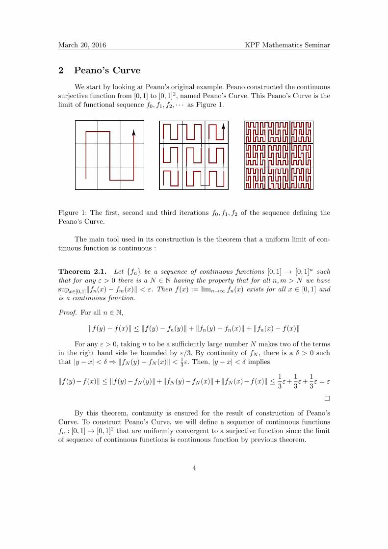
We start by looking at Peano’s original example. Peano constructed the continuoussurjective function from [0, 1] to [0, 1]2, named Peano’s Curve. This Peano’s Curve is thelimit of functional sequence f0, f1, f2, · · · as Figure 1.

Figure 1: The first, second and third iterations f0, f1, f2 of the sequence defining thePeano’s Curve.

The main tool used in its construction is the theorem that a uniform limit of con-tinuous function is continuous :

Theorem 2.1. Let {fn} be a sequence of continuous functions [0, 1] → [0, 1]n suchthat for any ε > 0 there is a N ∈ N having the property that for all n,m > N we havesupx∈[0,1]‖fn(x) − fm(x)‖ < ε. Then f(x) := limn→∞ fn(x) exists for all x ∈ [0, 1] andis a continuous function.

Proof. For all n ∈ N,

‖f(y)− f(x)‖ ≤ ‖f(y)− fn(y)‖+ ‖fn(y)− fn(x)‖+ ‖fn(x)− f(x)‖

For any ε > 0, taking n to be a sufficiently large number N makes two of the termsin the right hand side be bounded by ε/3. By continuity of fN , there is a δ > 0 suchthat |y − x| < δ ⇒ ‖fN (y)− fN (x)‖ < 1

3ε. Then, |y − x| < δ implies

‖f(y)−f(x)‖ ≤ ‖f(y)−fN (y)‖+‖fN (y)−fN (x)‖+‖fN (x)−f(x)‖ ≤ 1

3ε+

1

3ε+

1

3ε = ε

By this theorem, continuity is ensured for the result of construction of Peano’sCurve. To construct Peano’s Curve, we will define a sequence of continuous functionsfn : [0, 1]→ [0, 1]2 that are uniformly convergent to a surjective function since the limitof sequence of continuous functions is continuous function by previous theorem.

4


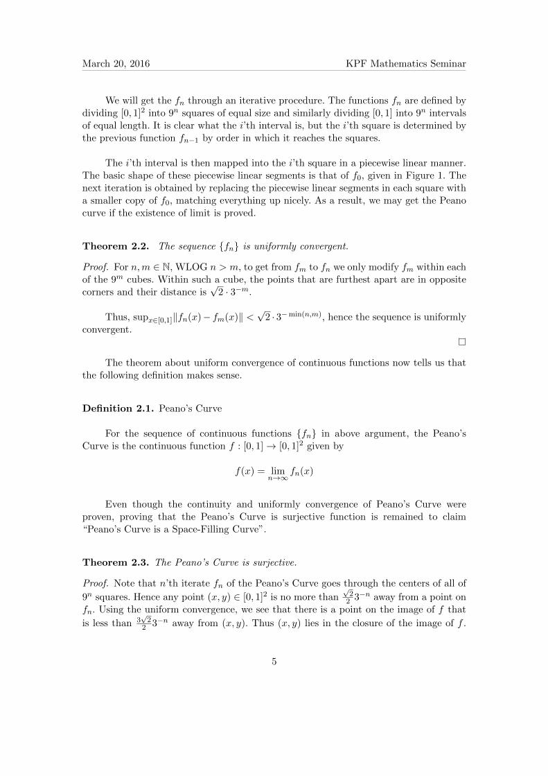
We will get the fn through an iterative procedure. The functions fn are defined bydividing [0, 1]2 into 9n squares of equal size and similarly dividing [0, 1] into 9n intervalsof equal length. It is clear what the i’th interval is, but the i’th square is determined bythe previous function fn−1 by order in which it reaches the squares.

The i’th interval is then mapped into the i’th square in a piecewise linear manner.The basic shape of these piecewise linear segments is that of f0, given in Figure 1. Thenext iteration is obtained by replacing the piecewise linear segments in each square witha smaller copy of f0, matching everything up nicely. As a result, we may get the Peanocurve if the existence of limit is proved.

Theorem 2.2. The sequence {fn} is uniformly convergent.

Proof. For n,m ∈ N, WLOG n > m, to get from fm to fn we only modify fm within eachof the 9m cubes. Within such a cube, the points that are furthest apart are in oppositecorners and their distance is

√2 · 3−m.

Thus, supx∈[0,1]‖fn(x)− fm(x)‖ <√

2 · 3−min(n,m), hence the sequence is uniformlyconvergent.

The theorem about uniform convergence of continuous functions now tells us thatthe following definition makes sense.

Definition 2.1. Peano’s Curve

For the sequence of continuous functions {fn} in above argument, the Peano’sCurve is the continuous function f : [0, 1]→ [0, 1]2 given by

f(x) = limn→∞

fn(x)

Even though the continuity and uniformly convergence of Peano’s Curve wereproven, proving that the Peano’s Curve is surjective function is remained to claim“Peano’s Curve is a Space-Filling Curve”.

Theorem 2.3. The Peano’s Curve is surjective.

Proof. Note that n’th iterate fn of the Peano’s Curve goes through the centers of all of

9n squares. Hence any point (x, y) ∈ [0, 1]2 is no more than√22 3−n away from a point on

fn. Using the uniform convergence, we see that there is a point on the image of f that

is less than 3√2

2 3−n away from (x, y). Thus (x, y) lies in the closure of the image of f .

5


Since the image of the compact set under any continuous function is compact and henceclosed, as (x, y) in fact lies in the image of f . Therefore, f is surjective.

To sum up, the Peano’s Curve, constructed during this section, is a surjecttivecontinuous function [0, 1]→ [0, 1]2.

“Therefore, Peano’s Curve is a Space-Filling Curve.”

Note that though each of fn is injective, the limit f is not. This is will proven later,as a consequence of one of the intermediate results in the proof of the Hahn-MazurkiewiczTheorem.

3 Lebesgue’s Curve

We will now give a second construction of a Spcae-Filling Curve, due to Lebesgue in1904. The ideas in this construction will play an important role in the proof of the Hahn-Mazurkiewicz Theorem, and along the way we will meet an interesting space known asa Cantor space.

Lebesgue’s Curve will be clearly surjective, because it will be given by connectingthe point in the image of a surjective map from a subset of [0, 1] by linear segments.This subset is the Cantor set :

Definition 3.1. Cantor set

Let C, the Cantor set, be the subset of [0, 1] by deleting all elements that have a 1in their ternary decimal expansion.

Alternatively, C is given by the repeatedly removing middle thirds of intervals. Onestarts with C0 = [0, 1], C1 = [0, 1/3] ∪ [2/3, 1], etc., and sets C =

⋂Cn. Lebesgue then

defined the following function from C to [0, 1]2 :

l

( ∞∑i=1

2ai3i

)=

( ∞∑i=1

a2i−1

2i,∞∑i=1

a2i2i

)This is easily seen to be surjective. We will show it is continuous.

6


Theorem 3.1. The function l is continuous.

Proof. If |y − x| < 1/32n+1(i.e. our δ), then the first 2n ternary decimals are the same.Hence the first n binary decimals of the x and y−coordinate of l(x) and l(y) are thesame. This implies that they are no further that

√2/2n(i.e. our ε) apart.

Now Lebesgue extends this function linearly over the gaps in [0, 1] left by the Can-tor set. We denote such a gap by (an, bn). Then we obtain l̃ : [0, 1]→ [0, 1]2 as follows

l̃(x) =

{l(x) if x ∈ C(l(bn)− l(an)) x−anbn−an + l(an) if x ∈ (an, bn) ⊂ [0, 1] \ C

We claim that this function is continuous. Clearly it is continuous on the gaps(an, bn) in the complement of the Cantor set because it is linear there. It is however notclear it continuous at the points of the Cantor set. However, by continuity of l and thefact that linear interpolations do not get far from their endpoints, we will also be ableto prove continuity there.

Theorem 3.2. The function l̃ is continuous.

Proof. By the remarks above it suffices to prove continuity at x ∈ C. Since C has emptyinterior or equivalently every point is a boundary point, there are three situations :

1. x is both on the left and the right a limit of points in C

2. x borders a gap (an, bn) on the left

3. x borders a gap (an, bn) on the right

We will do the last case and skip the first two, because they are very similar to thelast case.

We do not need to consider about continuity from the right, as l̃ is linear there. Wecan take a δ satisfying 0 < δ < 1/32n+1 and such that if y < x and |y − x| < δ, then ylies in C or in a gap (ak, bk) such that |ak − x| < 1/32n+1. The idea is just to take δ abit smaller than 1/32n+1 such that [x− 1/32n+1, x− δ] contains an element of C.

Then, if y ∈ C, then we know that∥∥l̃(y)− l̃(x)

∥∥ =∥∥l(y)− l(x)

∥∥ <√

2/2n bythe Theorem 3.1. If y /∈ C, then y lies in another gap (ak, bk) with x ≤ ak and|ak − x| < 1/32n+1. Note that l̃(y) = (l(bk) − l(ak))

y−akbk−ak + l(ak). With this notice,∥∥l̃(y)− l̃(x)

∥∥ < √2/2n now follows by the convexity of balls in Euclidean space : If the

7


endpoints of a line segment lie in a ball, then the entire line segment lies in the ball.

Since |ak − x| < 1/32n+1 and |bk − x| < 1/32n+1, l̃(ak) and l̃(bk) are in the ballB√2/2n(l̃(x)) by the Theorem 3.1. Thus,

∥∥l̃(y)− l̃(x)∥∥ < √2

2n

since l̃(y) lies on the line segment whose endpoints are l̃(ak) and l̃(bk). Therefore, l̃ iscontinuous.

To sum up, the Lebesgue’s Curve, constructed during this section, is a surjectivecontinuous function [0, 1]→ [0, 1]2.

“Therefore, Lebesgue’s Curve is a Space-Filling Curve.”

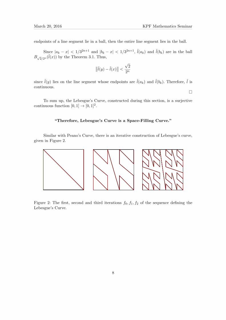
Similar with Peano’s Curve, there is an iterative construction of Lebesgue’s curve,given in Figure 2.

Figure 2: The first, second and third iterations f0, f1, f2 of the sequence defining theLebesgue’s Curve.

8


4 The Hahn-Mazurkiewicz Theorem

In this section we prove the Hahn-Mazurkiewicz Theorem for subsets of Euclideanspace. Before we begin, let us define some basic topological concepts.

Definition 4.1. For a subset A of Rn,

1. A is compact if each of its open covers has a finite subcover.

Equivalently, we can define compactness if every sequence has a convergent subse-quence with limit in A.

Furthermore, by Heine–Borel Theorem, A ⊂ Rn is compact iff it is bounded andclosed.

2. A is connected if we can’t write it A = (U∪V )∩A, where U and V are non-emptydisjoint open subsets of Rn.

3. For x ∈ A, the set Cx = {y ∈ A | ∃X ⊂ A s.t. x, y ∈ X and X is connected} isconnected component of x.

4. A is path-connected if any two points can be joined a continuous path withimage in A.

5. A is uniformly path-connected if for all ε > 0 there exists a η ∈ (0, ε) suchthat if a, a′ ∈ A satisfy

∥∥a′ − a∥∥ < η, then there is a continuous path with imagein Bε(a

′) ∩Bε(A) ∩A connecting a′ and a.

6. A is weakly locally-connected at x ∈ A if for every open set V containing xthere exists a connected subset U of V such that x lies in the interior of U .

7. A is weakly locally-connected if it is weakly locally-connected at x for everyx ∈ A.

Equivalently, it is said to be weakly locally-connected if for all x ∈ A and ε > 0we can find a smaller δ > 0 such that a ∈ Bδ(x), then x and a lie in the sameconnected component of A ∩Bε(x).

Note that connected set may not imply weakly locally-connected, vice versa. Forexample, set of two disjoint disks is weakly locally-connected but not connected. Inaddition, Topologist’s sine curve is connected but not weakly locally-connected. Withthis basic topological concepts, we will derive the final goal, the Hahn-MazurkiewiczTheorem.

9


Theorem 4.1. The Hahn-Mazurkiewicz Theorem

A subset A ⊂ Rn is the image of some continuous map f : [0, 1]→ Rn if and onlyif it is compact, connected and weakly locally-connected.

We will split the proof into two parts. The easier implication is that the image of aSpace-Filling Curve is compact, connected and locally-connect, i.e. that our conditionsare necessary. For the converse we’ll have to work a bit harder. The trick is to mimicLebesgue’s construction in general, using Hausdorff’s theorem on the images of theCantor set.

4.1 The conditions are necessary.

We will start by proving that the conditions of compactness, connectedness andweakly locally-connectedness are necessary.

Theorem 4.2. The image of a continuous map f : [0, 1] → Rn is compact, connectedand weakly locally-connected.

Proof. For image A, let an be a sequence in A. Then, by picking a point in each preimageof an an we get a sequence xn in [0, 1]. Since [0, 1] is compact, there is a convergent sub-sequence xnk

in [0, 1], with limit x. We claim that the ankconverge for f(x). But this is

a direct consequence of the continuity of f : it sends convergent sequences to convergentsequences.

The image of a path-connected set is clearly path-connected. But path-connectedimplies connected, so A is in fact connected.

For weakly locally-connectedness we have to a bit more careful. Suppose that fora ∈ A the condition of weakly locally-connectedness fails. Then we can find an ε > 0and ηn < ε with ηn → 0 and an ∈ Bηn(a) ∩ A such that an and a don’t lie in the sameconnected component of Bε(a). Note that by construction the sequence {an} convergesto a. Pick an element xn in the preimage of an. By compactness of [0, 1] this has aconvergent subsequence xnk

with limit x, which necessarily is mapped to a. There is aδ > 0 such that |y − x| < δ implies

∥∥f(y)− f(x)∥∥ < ε. Take K sufficiently large such

that |x − xnK | < δ. Then the entire line segment whose endpoints are xnK and x ismapped into Bε(a) ∩ A and hence anK and a lie in the same connected component ofBε(a) ∩A, contradicting our assumption on anK .

This theorem is generalized in point-set topology, where one proves that the imageof any compact, resp. connected space is compact, resp. connected.

10


4.2 Hausdorff’s theorem and a theorem on path-connectedness.

In this subsection we will prove Hausdorff’s theorem about the possible images inEuclidean space under a continuous map of the Cantor set. This was proven in 1927 byHausdorff and independently in 1928 by Alexandroff. It says, in some sense, that theCantor set is the universal compact subset of Euclidean space of any dimension.

Theorem 4.3. Hausdorff’s theorem

Every compact subset of Rn is a continuous image of the Cantor set.

Proof. Let A be our compact set. Consider the cover of A given by B1(a) for a ∈ A.By compactness there is a finite subcover, which by duplicating elements of the cover ifnecessary is of the form B1(ai) for 1 ≤ i ≤ 2n1 . Now cover Ai = B̄1(ai) ∩ A by B1/2(a)for a ∈ B1(ai) ∩ A and by duplicating elements of the finitely many covers if necessarywe can assume it has a finite subcover B1/2(ai,j) for 1 ≤ i ≤ 2n1 and 1 ≤ j ≤ 2n2 with n2independent of i. We set Ai,j = B̄1/2(ai,j)∩ B̄1(ai)∩A. Continue this procedure, makingthe radius of the balls half as large each step.

Notice that for a sequence ki ∈ {1, · · · , 2ni} we get a sequence of nested closedsets with radius going to 0. This determines a unique element of A as follows : a is theunique element of

⋂iAk1,k2,··· ,ki . Since we are dealing with increasingly fine covers and

every element of A lies in some intersection of elements of the cover, we obtain eachelement of A this way. For convenience, we define a way of getting from a sequence{an}n∈N of 0, 1’s to a sequence of numbers {Kn}n∈N in {1, · · · , 2ni}. They are given byKi =

∑nij=1 aj+n1+···+ni−12j−1. Now, we will define a function f : C → A given by

f

( ∞∑i=1

2ai3i

)= unique element of

⋂i

AK1,K2,··· ,Ki

This is surjective by the previous remark about every element lying in an inter-section of some elements of the cover. We also claim it is continuous. This is actuallyrather simple : if |y − x| < 3n+1 then the first n digits in the ternary expansion areequal. We can find a j such that n1 + n2 + · · · + nj ≤ n ≤ n1 + n2 + · · · + nj+1. Thusf(y) and f(x) lie in the same Ak1,k2,··· ,kj , which lies in a ball of radius 1/2k−1. Hence∥∥f(y)− f(x)

∥∥ < 1/2k−1 and we conclude that f is continuous.

We want to construct our Space-Filling Curve using this map, by connecting usingpaths in A over the gaps in the Cantor set. However, to be able to do this we need tofind such paths and show they can be chosen sufficiently short for points in A that areclose together.

11


Before beginning the next subsection, note that below theorem without proof.

Theorem 4.4. If A is compact, connected and weakly locally-connected, it is path-connected and uniformly path-connected.

4.3 The conditions are sufficient.

Now we’ll combine Hausdorff’s theorem and our theorem on path-connectedness toconstruct a surjective map [0, 1]→ A under the conditions listed before. As said before,the idea is to copy the idea of Lebesgue’s construction of a Space-Filling Curve : useHausdorff’s theorem to get a surjective map from the Cantor set into A and use ourtheorem on path-connectedness to prove that we can connect the image by paths overthe gaps in the Cantor set.

Theorem 4.5. If A ⊂ Rn is compact, connected and weakly locally-connected, then thereexists a surjective continuous function f : [0, 1]→ A.

Proof. Since A is compact, by Hausdorff’s theorem there exists a continuous surjectivefunction g : C → A.

By the Theorem 4.4, A is uniformly path-connectedness so that we can find a de-creasing sequence of ηn such that

∥∥a′ − a∥∥ < ηn implies that there is a continuous pathwith image in B1/2n(a)∩B1/2n(a′)∩A. By continuity of g and compactness of C, we can

find a decreasing sequence of δn > 0 such that |y − x| < δn implies∥∥g(y)− g(x)

∥∥ < ηn.

If (ak, bk) is a gap in C such that δn+1 ≤ |bk−ak| < δn, then we can find a continuouspath γk : [ak, bk] → A such that γk lies in B1/2n(g(ak)) ∩ B1/2n(g(bk)) ∩ A connectingg(ak) to g(bk). We define f as follows :

f(x) =

{g(x) if x ∈ Cγk if x ∈ (ak, bk) ⊂ [0, 1] \ C

This function is clearly continuous at all points of [0, 1]\C and as before the pointsx ∈ C comes in three types :

1. x is both on the left and the right a limit of points in C

2. x borders a gap (an, bn) on the left

3. x borders a gap (an, bn) on the right

Again we will do the last case and skip the first two, because they are very similarto the last case.

12


Continuity from the right is obvious, as f is just a continuous path there. Forcontinuity from the left pick δ > 0 satisfying δn > δ > 0 and such that if y < x and|y − x| < δ, then y ∈ C or it lies in a gap (ak, bk) such that |ak − x| < δn.

If y ∈ C, then |y − x| < δn and hence∥∥f(y)− f(x)

∥∥ =∥∥g(y)− g(x)

∥∥ ≤ ηn. Ify /∈ C, then y lies on a path that does not get further than 1/2n from g(x) and hence∥∥f(y)− f(x)

∥∥ ≤ 1/2n. So given an ε > 0 just take a n ∈ N so that min{ηn, 1/2n} < εand set δ = δn. Then |y − x| < δ implies

∥∥f(y)− f(x)∥∥ < ε.

As a result, Hahn-Mazurkiewicz Theorem is proven so that we can decide theexistence of Space-Filling Curve in given subset of Euclidean space. Namely, we cancharacterize subsets of Euclidean spcae that there exists a Space-Filling Curve as :

“Space-Filling Curve exists in the subset of Euclidean spaceif and only if it is compact, connected and weakly locally-connected.”

13

Documents

Existence of Space-Filling Curve in Euclidean Spacemathsci.kaist.ac.kr/~kdryul/files/talks/Existence of Space-Filling... · Existence of Space-Filling Curve in Euclidean Space Kim,