Exercise 8 - Snow - US EPA · BASINS/HSPF Training Exercises 8-1 Exercise 8 – Simulation of Snow Accumulation and Melt

BASINS/HSPF Training Exercises

8-1

Exercise 8 – Simulation of Snow Accumulation and Melt

Water Quality Calibration/ V alidation

Parameter Development/Model

Setup

H yd r ologic Ca lib r a t ion /

Va lida t ion

T imeseries Data M anagement

Study Definition/Modeling

StrategyScenario A nalysis

BASINS/HSPF Application Steps

Water Quality Calibration/ V alidation

Parameter Development/Model

Setup

H yd r ologic Ca lib r a t ion /

Va lida t ion

T imeseries Data M anagement

Study Definition/Modeling

StrategyScenario A nalysis

BASINS/HSPF Application Steps

Question addressed in this section:

1) How do I add snow simulation to my model? 2) How do I simulate snow in HSPF using the degree-day approach? 3) What parameters will affect snow depth, snowmelt, and flow using the degree-

day approach? 4) How do I simulate snow in HSPF using an energy balance approach? 5) What parameters will affect snow depth, snowmelt, and flow using the energy

balance approach?

The SNOW module simulates snowmelt contributions from the land surface derived from the fall, accumulation, and melting of snow. This module is necessary for a complete hydrologic package since much of the runoff, particularly in the northern half of the United States, is directly related to snow conditions.

Two options are available for modeling the processes involved in snow accumulation and melt on a land segment: an energy balance and a degree-day approach. The energy balance approach is based on work by the Corps of Engineers (1956), Anderson and Crawford (1964), and Anderson (1968). Empirical relationships are employed when physical relationships are not well understood. The snow algorithms use meteorological data to: determine whether precipitation occurs as rain or snow; simulate an energy balance for the snow pack; determine the effect of the heat fluxes on the snow pack, and; calculate the resulting melt that reaches the land surface.

The second snowmelt method uses a temperature index, or "degree-day" approach. Most processes from the snow algorithms are employed; however, snowmelt due to atmospheric heat exchange is calculated using the air temperature and an empirical degree-day factor. This approach minimizes the requirements for meteorological data to precipitation and air temperature. The reader is referred to Rango and Martinec (1995) for a summary of the degree-day method. SNOW may require six meteorological time series for each land segment simulated, depending on the option chosen. They are:


8-2

Meteorological Quantity Energy balance Temperature Index (Degree-Day)

Precipitation required required Air temperature required required Solar radiation required not used

Dew point required optional Wind velocity required not used Cloud cover optional not used

A value from each of these time series is input to SNOW at the start of each simulation interval. However, some of the meteorological time series are only used intermittently for calculating rates. One such example is the calculation of the potential rate of evaporation from the snow pack.

Air temperature is used to determine whether precipitation is falling as rain or as snow. The critical temperature TSNOW may be automatically adjusted upward by up to one degree in unsaturated conditions, based on the dew point. This adjustment is optional when using the temperature index method, and is made only if the input dew point time series is supplied (Bicknell et al., 2001).

A. Simulating Snow using the Degree-Day Approach We are using the Norwalk watershed in Connecticut for the snow simulation/calibration exercise. The following map will help orient you in the watershed. Key locations that are referenced throughout the exercise are labeled.


8-3

QUESTIONS ANSWERED: 1) How do I add snow simulation to my model? 2) How do I simulate snow in HSPF using the degree-day approach? 3) What parameters will affect snow depth and flow using the degree-day approach? 1. From the Start menu under Programs, select BASINS and then WinHSPF.

2. From the File menu, select Open.

3. Navigate to c:\basins\modelout\snow and select “Nor_hyd.uci.” Click OPEN.

Note: For simplification purposes, we have already turned on the “SNOW” module,

entered values for key snow parameters, and specified output for this simulation. In the following steps (4-21), we will briefly show you what has previously been done in preparation for snow calibration. The steps are provided for informational purposes – you will not need to make any changes.

4. Click the “Control Cards” button, .

5. When the “Control Window Selection” window appears, click DESCRIPTIONS. The following window will appear:

6. Make sure the “Pervious Land” tab is selected. Notice that the boxes beside “ATEMP”, “SNOW”, and “PWATER” are checked (selected). Note: The “ATEMP” module modifies the input air temperature to represent the

mean air temperature for the land segments. This correction is needed because the subwatersheds are at significantly higher elevations than the temperature gage.

7. Click the “Impervious Land” tab. Notice that the “ATEMP”, “SNOW”, and

“IWATER” modules are checked.

8. Click OK or CANCEL.


8-4

9. Click the “Input Data Editor” button, .

10. Double click PERLND SNOW SNOW-FLAGS. Click OK if asked whether to add the table.

11. Click in the first cell in the “SNOPFG” column. Enter “1” and double click the column heading to copy the value to the rest of the cells in the column.

Note: The value of SNOPFG determines which method will be used to compute

snow accumulation and melt. A value of “0” means that the atmospheric heat exchange portion of snowmelt will be based on the energy balance; “1” means it will be based on a degree-day factor. The default method for computing snow accumulation and melt is the energy balance approach. The degree-day approach is more commonly used in other models because it requires less input data; it is also easier to calibrate due to fewer calibration parameters. For this reason, this exercise will begin by covering the degree-day approach and then cover the energy balance approach. Only a few of the key degree-day approach parameters will be covered in this section. The next section, on the energy balance approach, will cover the other calibration parameters that are common to both the degree-day and energy balance approaches along with those associated only with the energy balance approach.

12. Click APPLY.

13. Click OK. 14. Double click IMPLND SNOW SNOW-FLAGS. Click OK if asked whether to

add the table.


16. Click APPLY.

17. Click OK.

18. Click CLOSE.

19. Click the “Output Manager” button, . 20. Click the button beside “Other.” The following window will appear:


8-5

Note: PERLND 301 and PERLND 302 refer to forest and agriculture, respectively. “SNOW:PDEPTH” specifies that snow depth output will be produced for these two pervious land segments. Snow depths will typically be simulated differently for each land use category because elevation (and the corresponding air temperature) varies with land use category. Also, the effective shading of incident solar radiation (i.e., SHADE parameter) will vary with the vegetation and topography (e.g., north-facing slopes having higher SHADE values than south-facing slopes). In reality, you would want to add PDEPTH for all the PERLNDs and IMPLNDs modeled. We are only looking at two landuses for simplification purposes.

21. Click CLOSE. Now that we have briefly showed you what steps have been taken in preparation for snow calibration, we will run the model and view the results in GenScn to determine what kinds of parameter adjustments might be helpful in improving the flow simulation. First, we will need to change KMELT, the key calibration parameter in the degree-day approach that controls snow melt, to a non-zero value.

22. Click on the “Input Data Editor” button, .

23. Double click PERLND SNOW SNOW-PARM1.

24. Change each value in the “KMELT” column to “0.02.” Note: KMELT is the constant degree-day factor for the temperature index snowmelt

method. It is used when SNOPFG=1 and VKMFG=0 (see VKMFG explanation below) in the SNOW-FLAGS table. KMELT can be input on a monthly basis to reflect differences in melt conditions (for example, radiation, wind movement, etc.) during early and late winter periods that are not adequately accounted for as a function of only temperature. Increasing this parameter will increase the rate of snowmelt.


8-6

Note: If VKMFG is 1, the degree-day factor (KMELT) can vary monthly. If it is “0,” an annual value will be used.

25. Click APPLY. 26. Click OK. 27. Double click IMPLND SNOW SNOW-PARM1.

28. Change each value in the “KMELT” column to “0.02.” 29. Click APPLY.

30. Click OK. 31. Click CLOSE.

32. Click the “Run HSPF” button, . 33. Click SAVE/RUN.

34. Click the “View Output through GenScn” button, .

35. Select the “HSPF Output” tab and make sure “c:\BASINS\modelout\snow\ct.wdm” is checked.

36. Click OK. 37. In the “Scenarios” frame, select “NORWBASE” and “OBSERVED.”

38. In the “Constituents” frame, select “SNWD.”

Note: “SNWD” is the snow depth identifier (inches).

39. Click the “Add to Time Series List” button, . Three new records will appear in


8-7

the “Time Series” frame.

40. Select the time series corresponding to DSN numbers “22,” “1120,” and “1121” by holding the Shift key and clicking on each entry.

Note: The DSNs selected in this step correspond to the following constituents:

DSN Constituent 22 Observed snow depth at Bridgeport

1120 Simulated snow depth for PERLND 301 (forest) 1121 Simulated snow depth for PERLND 302 (agriculture)

41. Click the “Generate Graphs” button, .

42. In the “Graph” window, make sure “Standard” is checked. Click GENERATE. The following plot should appear:

Note: Notice that the output from PERLND 301 and 302 is similar. Also notice that we are over predicting the snow depth.

43. Do not close this plot. Toggle to the main GenScn screen. In the “Scenarios” frame,

select “NORWBASE” and “OBSERVED.”


8-8

44. In the “Constituents” frame, select “FLOW.”

45. Click the “Add to Time Series” button, .

46. Highlight the series that correspond to DSN numbers “23” and “1122” (by holding Shift and clicking on each entry). Note: The DSNs selected in this step correspond to the following:

DSN Constituent 23 Observed flow at South Willington

1122 Simulated flow for Reach 3 (Norwalk River)


48. In the “Graph” window, make sure “Standard” is checked and click GENERATE. Compare the flow plot to the snow depth plot:

KMELT = 0.02

Note: We have added precipitation and air temperature as auxiliary plots to each of

the flow/snow-depth comparison plots so that you can see when precipitation


8-9

occurs and how air temperature affects snow depth when using the degree-day approach. Also, we have cropped the plots and added them to the same window so that you can more easily compare them.

We will now look at two different winter periods to see how closely we are capturing snow accumulation and melt. 49. In the “Time Series” frame, highlight the records that correspond to the DSN

numbers “22,” “1120,” and “1121.”

50. In the “Dates” frame, change the “Start” and “End” dates to the following:


52. In the “Graph” window, make sure “Standard” is checked and click GENERATE.

53. Return to the main GenScn window. In the “Time Series” frame, highlight the flow records (DSN numbers “23” and “1122’).

54. Make sure the “Start” and “End” dates are as specified as shown above. Click the

“Generate Graphs” button, .

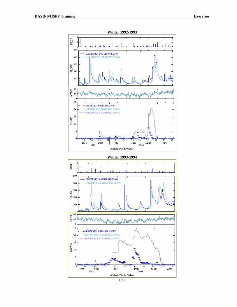
55. In the “Graph” window, make sure “Standard” is checked and click GENERATE. 56. Repeat these steps (51-56) for 1993/11/15 to 1994/04/15. Your plots should look like

the following:

Winter 1992-1993


8-10


8-11

Winter 1993-1994

Note: Notice that we are generally underestimating most of the winter flows and spring runoff because too much snow is being accumulated and it is not melting at the appropriate time.

57. Close all plots, the “Graph” window, and GenScn. The snow depth gage that is nearest to our watershed is located in Bridgeport. Our watershed is farther inland and at significantly higher elevations than the snow depth gage. Keep in mind that our watershed will likely have higher observed snow depths than the values recorded at Bridgeport. However, the previous plots indicate that our simulated snow depths are much higher than the observed snow depths. We now need to make parameter adjustments that focus on reducing the amount of snow and subsequent snowmelt. After we adjust each key calibration parameter, we will assess whether the adjustments result in improved flow simulations – particularly runoff events due to snowmelt. We will also adjust meteorological data inputs to illustrate how they affect snow depth and snowmelt. The adjustments will not necessarily reflect the specific values needed for a better calibration, but they will illustrate trends and help you evaluate the types of parameter adjustments that can be considered.

58. Toggle to WinHSPF. Click on the “Input Data Editor” button, .


8-12


60. Change each value in the “KMELT” column to “0.05.” 61. Click APPLY. 62. Click OK. 63. Double click IMPLND SNOW SNOW-PARM1.

64. Change each value in the “KMELT” column to “0.05.” 65. Click APPLY.

66. Click OK. 67. Click CLOSE. 68. Following the steps you went through previously, run the simulation and plot the

snow depth and flow values in GenScn for the 1991/1/1 to 1995/12/31. Your plots should look like the following:

KMELT = 0.05

Note: You may need to edit the format of your plot (e.g., change the “line type” to

“thin” and the “marker type” to “none”) so that your plots look like those


8-13

shown above or below. Note: Note that the simulated snow depths now look similar to the observed snow

depths. Next, we need to look at different winter periods to see how closely we are capturing snowmelt.

69. In the “Time Series” frame, highlight the records that correspond to the DSN

numbers “22,” “1120,” and “1121.”




73. Return to the main GenScn window. In the “Time Series” frame, highlight the flow records (DSN numbers “23” and “1122’).

74. Make sure the “Start” and “End” dates are as specified as shown above. Click the

“Generate Graphs” button, .

75. Repeat these steps for 1993/11/15 to 1994/04/15. Your plots should look like the following:


8-14

Winter 1992-1993

Winter 1993-1994


8-15

Note: Although the snowmelt rate is slightly better than before, the snowmelt rate is still too slow. We will drastically increase the value of KMELT to test its sensitivity.

76. Close all plots, the “Graph” window, and GenScn.

77. Toggle to WinHSPF. Click on the “Input Data Editor” button, .


79. Change each value in the “KMELT” column to “0.9.”

80. Click APPLY.

81. Click OK.

82. Run the simulation and plot the snow depth and flow values in GenScn for the following periods: 1992/11/01 to 1993/04/30 and 1993/11/15 to 1994/04/15. Your plots should look like the following:

Winter 1992-1993

Winter 1993-1994

Too high

Too low


8-16

Note: Notice that the spring runoff is too early and that our simulated snow depths are similar to the observed snow depths, but our simulation is still missing many of the trends in the observed data.

83. Continue to adjust the KMELT parameter. You may want to add monthly values for

KMELT (see note below). See how well you can calibrate the snow depth and reach flow simulations using the degree-day approach by just changing the KMELT.

Note: Before adding monthly values, you must specify that you will vary the degree-

day factor monthly. The table for this is located in the “Input Data Manager” under PERLND SNOW SNOW-FLAGS. Change each of the values in the “VKMFG” column to “1.” The table in which you can enter the monthly values is located in the “Input Data Manager” under PERLND SNOW MON-MELT-FAC.

Note: You can also vary the values of TSNOW, SNOWCF, COVIND, MWATER,

and MGMELT to assist in refining the simulated snow accumulation and melt results. These parameters are further discussed in the energy balance section below.


8-17

84. Close all plots and GenScn. Before beginning the next section, you may want to change your KMELT values to 0.9. This will ensure that your graphs look like those in the following steps.

Air temperature is also a key input in simulating snow using the degree-day approach. HSPF already accounts for changes in air temperature as a result of elevation variations. Depending on the location weather station, the air temperature may require additional adjustments to reflect the conditions in the area being modeled. These adjustments can be made by changing the “MultFact” or multiplicative factor for input air temperature timeseries. Because snowmelt due to atmospheric heat exchange is calculated using the air temperature (and an empirical degree-day factor), increasing the “MultFact” value for “ATMP” will increase input air temperature and therefore, increase the simulated rate of snowmelt. Adjusting “MultFact” will allow us to examine the impacts of variations (and associated uncertainty) in meteorological conditions on the model results. Note that the “MultFact” is not considered a calibration parameter. It should only be adjusted if there is evidence suggesting that the air temperature inputs require some adjustment.

85. Toggle to WinHSPF. Click the “Input Data Editor” button, .

86. Double click EXT SOURCES. Change the “MultFact” value for “ATMP” to “0.9” (from “1”).

Note: You will have to change the “MultFact” value for “ATMP” for each PERLND

and IMPLND. This means you will need to scroll down and change the “ATMP” value that corresponds with PERLND 101, 102, 103, 104, 201, 202, 203, 204, 301, 302, 303, 304 and IMPLD 101, 102, 201, 202, 301, 302.

87. Click APPLY.

88. Click OK.

89. Click CLOSE.

90. Click the “Run HSPF” button, .

91. Click SAVE/RUN.

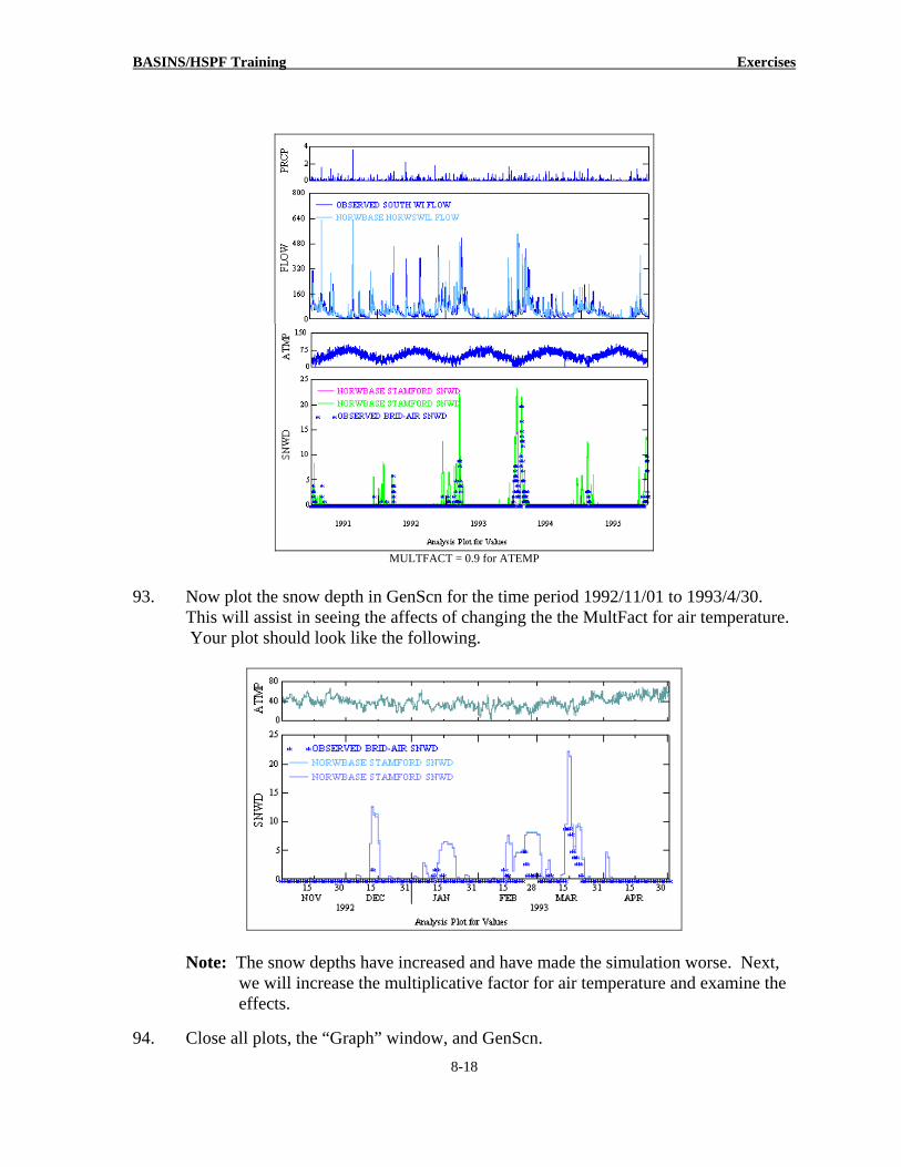
92. Plot the snow depth and flow in GenScn for the time period 1991/01/01 to 1995/12/31. Your plots should look similar to the following:


8-18

MULTFACT = 0.9 for ATEMP

93. Now plot the snow depth in GenScn for the time period 1992/11/01 to 1993/4/30.

This will assist in seeing the affects of changing the the MultFact for air temperature. Your plot should look like the following.

Note: The snow depths have increased and have made the simulation worse. Next, we will increase the multiplicative factor for air temperature and examine the effects.



8-19


96. Double click EXT SOURCES. Change the “MultFact” value for “ATMP” to “1.1” (from “0.9”).

Note: You will have to change the “MultFact” value for “ATMP” for each PERLND

and IMPLND. 97. Click APPLY.

98. Click OK.

99. Click CLOSE.

100. Run the simulation and plot the snow depth and flow in GenScn for the time period

1991/01/01 to 1995/12/31. Your plots should look similar to the following:

MultFact = 1.1 for ATMP

101. Plot the snow depth in GenScn for the time period 1992/11/01 to 1993/4/30. Your plot should look similar to the following:


8-20

Note: Notice that the snow depths decreased substantially and are within a closer

range of the observed data. 102. Close all plots, the “Graph” window, and GenScn.

B. Simulating Snow using an Energy Balance Approach QUESTIONS ANSWERED: 4) How do I simulate snow in HSPF using an energy balance? 5) What parameters will affect snow depth and flow using the energy balance approach?


2. Double click PERLND SNOW SNOW-FLAGS.


Note: A value of “0” for SNOPFG means that the atmospheric heat exchange portion

of snowmelt will be based on the energy balance.

4. Click APPLY.

5. Click OK. 6. Double click IMPLND SNOW SNOW-FLAGS. 7. Click in the first cell in the “SNOPFG” column. Enter “0” and double click the


8-21

column heading to copy the value to the rest of the cells in the column. 8. Click APPLY.

9. Click OK.

10. Click CLOSE.

11. Click the “Run HSPF” button, . 12. Click SAVE/RUN.

13. Click the “View Output through GenScn” button, .

14. In the “Scenarios” frame, select “NORWBASE” and “OBSERVED.”

15. In the “Constituents” frame, select “SNWD.”

Note: “SNWD” is the snow depth identifier (inches).

16. Click the “Add to Time Series List” button, . Three new records will appear in the “Time Series” frame.

17. Select the time series corresponding to DSN numbers “22,” “1120,” and “1121.”


8-22

Note: The DSNs selected in this step correspond to the following constituents:

DSN Constituent 22 Observed snow depth at Bridgeport

1120 Simulated snow depth for PERLND 301 (forest) 1121 Simulated snow depth for PERLND 302 (agriculture)


19. In the “Graph” window, make sure “Standard” is checked. Click GENERATE. The following plot should appear:

20. Do not close this plot. Toggle to the main GenScn screen. In the “Scenarios” frame,

select “NORWBASE” and “OBSERVED.”

21. In the “Constituents” frame, select “FLOW.”

22. Click the “Add to Time Series” button, .

23. Highlight the series that correspond to DSN numbers “23” and “1122.” Note: The DSNs selected in this step correspond to the following:

DSN Constituent 23 Observed flow at South Willington

1122 Simulated flow for Reach 3 (Norwalk River)


8-23


25. In the “Graph” window, make sure “Standard” is checked and click GENERATE. Compare the flow plot to the snow depth plot:

26. Close all plots and the “Graph” window.

Next, we will examine the snow depth and reach flow for individual winter periods. 27. In the “Time Series” frame, highlight the records that correspond to the DSN

numbers “22,” “1120,” and “1121.”




8-24


31. Return to the main GenScn window. In the “Time Series” frame, highlight the flow

records (DSN numbers “23” and “1122’).

32. Make sure the “Start” and “End” dates are as specified in Step 31.Click the “Generate

Graphs” button, .

33. In the “Graph” window, make sure “Standard” is checked and click GENERATE. Compare the snow depth plot to the flow plot to assess how differences in the snow simulation contribute to differences in the flow simulations.

Note: The model has significantly over-predicted the snow-depth for March.

34. Close the plots and the “Graph” window.

35. Look at the snow depth and flow data plots for the following time period:


8-25

Your plots should look like the following:

Note: Similar to the previous section, these and previous plots indicate that our simulated snow depths are generally much higher than the observed snow depths. Our parameter adjustments should focus on reducing the amount of snow and subsequent snowmelt. After we adjust key parameters, we will assess whether the adjustments result in improved flow simulations – particularly runoff events due to snowmelt. Also, we will adjust meteorological data inputs and various parameters to illustrate how they affect snow depth and snowmelt. As stated previously, adjustments won’t necessarily reflect the specific values needed for a better calibration, but they will illustrate trends and help you evaluate the types of parameter adjustments that can be considered.



38. Double click EXT SOURCES. We will leave the “MultFact” value for “ATMP” at “1.1.”

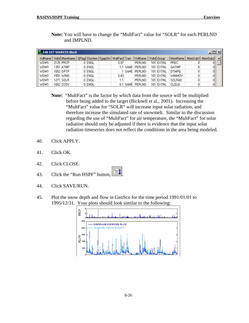
39. Change the “MultFact” value for “SOLR” to “1.1” (from “1”).


8-26

Note: You will have to change the “MultFact” value for “SOLR” for each PERLND and IMPLND.

Note: “MultFact” is the factor by which data from the source will be multiplied before being added to the target (Bicknell et al., 2001). Increasing the “MultFact” value for “SOLR” will increase input solar radiation, and therefore increase the simulated rate of snowmelt. Similar to the discussion regarding the use of “MultFact” for air temperature, the “MultFact” for solar radiation should only be adjusted if there is evidence that the input solar radiation timeseries does not reflect the conditions in the area being modeled.

40. Click APPLY.

41. Click OK.

42. Click CLOSE.

43. Click the “Run HSPF” button, .

44. Click SAVE/RUN.



8-27

MULTFACT = 1.1 for ATEMP and SOLR


MultFact = 1.1 for ATMP & SOLR

47. Plot the snow depth and flow in GenScn for the time period 1993/12/01 to

1994/03/31. Your plots should look similar to the following:


8-28


Note: The snow depths haven’t changed significantly, but there is a slight difference in reach flow. Next, we will decrease the multiplicative factor for air temperature and solar radiation, and examine the effects.



50. Double click EXT SOURCES. Change the “MultFact” value for “ATMP” to “0.9” (from “1.1”).

51. Change the “MultFact” value for “SOLR” to “0.9” (from “1.1”). Note: You will have to change the “MultFact” value for “SOLR” for each PERLND

and IMPLND.

52. Click APPLY.

53. Click OK.

54. Click CLOSE. 55. Run the simulation and plot the snow depth and flow in GenScn for the time period

1992/11/01 to 1993/04/30. Your plots should look similar to the following:


8-29






8-30


59. Double click EXT SOURCES. Change the “MultFact” value for “ATMP” back to “1” (from “0.9”).

60. Change the “MultFact” value for “SOLR” to “1” (from “0.9”).

61. Click APPLY.

62. Click OK.


64. Click in the first cell in the “SNOWCF” column. Change the value to “1” and double click the column heading to copy the value to the rest of the cells in the column. Your screen should look like the following:

Note: SNOWCF is the factor by which the input precipitation data will be multiplied, if the simulation indicates it is snowfall, to account for poor catch efficiency of the gage under snow conditions. We will examine how simulated snow depth, snowmelt volumes, and reach flow are affected when this parameter is adjusted.

65. Click APPLY.


68. Run the simulation and plot the snow depth and flow values in GenScn for the two

winter periods: 1992/11/01 to 1993/04/30 and 1993/11/15 to 1994/04/15. Your plots should look like the following:

Winter 1992-1993


8-31

SNOWCF = 1

Winter 1993-1994

SNOWCF = 1

Note: The simulated snow depths decreased significantly.

69. Exit all plots, the “Graph” window, and GenScn.


71. Double click PERLND SNOW SNOW-PARM1. 72. Click in the first cell in the “SNOWCF” column. Change the value to “1.5” and


8-32

double click the column heading to copy the value to the rest of the cells in the column.

73. Click APPLY.

74. Click OK. Click CLOSE.

75. Run the simulation and plot the snow depth and flow values in GenScn for the two winter periods: 1992/11/01 to 1993/04/30 and 1993/11/15 to 1994/04/15. Your plots should look like the following:

Winter 1992-1993

SNOWCF =1.5

Winter 1993-1994

SNOWCF = 1.5

Compare the snow depth plots for SNOWCF = 1 and 1.5. The following plots were prepared


8-33

to help you easily view the differences in simulated snow depth. In the interest of time, we have prepared graphs for only snow depth; however, you should also examine the differences in the reach flow plots. Notice the differences in the melt period of March and April.

Winter 1992-1993

SNOWCF = 1 SNOWCF = 1.5

Winter 1993-1994

SNOWCF = 1 SNOWCF = 1.5

Note: Raising the value of SNOWCF to “1.5” increased our simulated snow depth considerably. Since the plots indicate that setting the value of “SNOWCF” to “1” produces simulated snow depths that more closely resemble the observed data, we will change the value of SNOWCF back to “1” before continuing. In actual calibration, we would look at the storm flow water balance and consider how well various SNOWCF values improve the flow simulations – remember, our primary goal when modeling snow is to improve the hydrology simulations.

76. Exit all plots, the “Graph” window, and GenScn.

77. Toggle back to WinHSPF.


8-34

78. Click the “Input Data Editor” button, .


80. Change each value in the “SNOWCF” column to “1.”

81. Click APPLY.

82. Click OK.

83. Double click “SNOW-PARM2.”

84. Change each value of “TSNOW” to “34.” Note: Under saturated vapor pressure conditions (as represented by dew point

temperature), TSNOW is the air temperature below which precipitation will be snow. Under non-saturated conditions the temperature is automatically adjusted slightly. In the following steps, we will examine the impacts of increasing this value.

85. Click APPLY.

86. Click OK.

87. Click CLOSE.



8-35

Winter 1992-1993

TSNOW = 34

Winter 1993-1994

TSNOW = 34

Compare the snow depth plots for TSNOW =32 and 34 (see below).

Winter 1992 - 1993


8-36

TSNOW = 32 TSNOW = 34

Note: Notice that the simulated snow depths in the circled periods were increased,

and they remained the same during other periods. Increasing the value of “TSNOW” will only have a significant effect during periods when the temperature is near the TSNOW value.

Winter 1993-1994

TSNOW = 32 TSNOW = 34

Note: These plots indicate that there wasn’t a significant difference in the snow

depths. This might be due to colder temperatures during the 1993-1994 winter.




92. Click in the first cell in the “CCFACT” column. Change the value to “0.5” and double click the column heading to copy the value to the rest of the cells in the column.


8-37

Note: CCFACT is a parameter that adapts the snow condensation/convection melt

equation to field conditions. It is used only when SNOPFG=0 in the SNOW-FLAGS table. Decreasing the value of CCFACT decreases the simulated rate of melt, and increasing CCFACT increases the simulated rate of melt. We will examine the impacts of adjusting this parameter on simulated snow depth and reach flow.

Note: A SNOPFG value of “0” specifies that we will use the energy balance

approach rather than the degree-day approach to simulate snow accumulation and melt.

93. Click APPLY.

94. Click OK.


Winter 1992-1993

CCFACT = 0.5


8-38

Winter 1993-1994

CCFACT = 0.5

Compare the snow depth plots below for CCFACT =2 and 0.5 (see below).

Winter 1992-1993

CCFACT = 2 CCFACT = 0.5


8-39

Winter 1993-1994

CCFACT = 2 CCFACT = 0.5

Note: With a CCFACT value of “0.5,” simulated snow depth has a much higher

recession rate (the snow takes longer to melt) than when CCFACT was “2.” 96. Close all plots, the “Graph” window, and GenScn.

97. Toggle to GenScn. Click the “Input Data Editor” button, .


99. Click in the first cell in the “CCFACT” column. Change the value to “5” and double click the column heading to copy the value to the rest of the cells in the column.

100. Click APPLY.




Winter 1992-1993


8-40

CCFACT = 5

Winter 1993-1994

CCFACT = 5

Compare the snow depth plots for CCFACT = 0.5 and 5 (see below).

Winter 1992-1993


8-41

CCFACT = 0.5 CCFACT = 5

Winter 1993 - 1994

CCFACT = 0.5 CCFACT = 5

Note: With a CCFACT value of “5,” simulated snow depth has a much lower

recession rate (the snow melts more quickly) than when CCFACT was “0.5.”




107. Click in the first cell in the “MWATER” column. Change the value to “0.1” and double click the column heading to copy the value to the rest of the cells in the column.

Note: MWATER is the maximum water content of the snow pack, in depth of water

per depth of water equivalent. It specifies how much melt water can be stored in the pack before it is released into the ground. Increasing the value of MWATER will allow more storage and delay runoff.


8-42

108. Click APPLY.




Winter 1992-1993

MWATER = 0.1

Winter 1993-1994

MWATER = 0.1

Compare the snow depth plots for MWATER = 0.03 and 0.1.


8-43

Winter 1992-1993

MWATER = 0.03 MWATER = 0.1

Winter 1993-1994


Note: There isn’t a significant difference in the snowmelt plots, so we will compare

the reach flow plots to see if the simulation has improved. Winter 1992-1993



8-44

Winter 1992-1993


Note: Notice that the flow increased significantly during the period between January

15 and January 31 in 1994.




115. Click in the first cell in the “MGMELT” column. Change the value to “0.05” and double click the column heading to copy the value to the rest of the cells in the column.

Note: MGMELT is the maximum rate of snowmelt by ground heat (depth of water

per day). This value is applied when the snow pack temperature is at the freezing (melting) point. Increasing this value will increase the melting rate.

116. Click APPLY.

117. Click OK.



8-45

Winter 1992 – 1993

MGMELT =0.05

Winter 1992 – 1993

MGMELT =0.05

Compare the snow depth plots for MGMELT = 0.01 and 0.05.


8-46

Winter 1992-1993

MGMELT = 0.01 MGMELT = 0.05

Winter 1993-1994


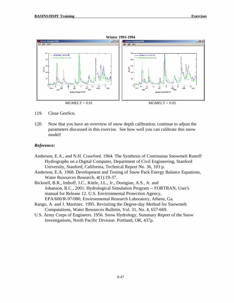
Note: Increasing MGMELT resulted in faster simulated melting rates. This made

the snow depth peak recessions steeper. Notice that the simulated snow depth, particularly in the circled regions, more closely resembles the observed snow depths.

Winter 1992-1993



8-47

Winter 1993-1994


119. Close GenScn.

120. Now that you have an overview of snow depth calibration, continue to adjust the

parameters discussed in this exercise. See how well you can calibrate this snow model!

Reference: Anderson, E.A., and N.H. Crawford. 1964. The Synthesis of Continuous Snowmelt Runoff

Hydrographs on a Digital Computer, Department of Civil Engineering, Stanford University, Stanford, California, Technical Report No. 36, 103 p.

Anderson, E.A. 1968. Development and Testing of Snow Pack Energy Balance Equations, Water Resources Research, 4(1):19-37.

Bicknell, B.R., Imhoff, J.C., Kittle, J.L., Jr., Donigian, A.S., Jr. and Johanson, R.C., 2001. Hydrological Simulation Program -- FORTRAN, User's manual for Release 12. U.S. Environmental Protection Agency, EPA/600/R-97/080, Environmental Research Laboratory, Athens, Ga.

Rango, A. and J. Martinec. 1995. Revisiting the Degree-day Method for Snowmelt Computations, Water Resources Bulletin, Vol. 31, No. 4, 657-669.

U.S. Army Corps of Engineers. 1956. Snow Hydrology, Summary Report of the Snow Investigations, North Pacific Division. Portland, OR, 437p.

Documents

Exercise 8 - Snow - US EPA · BASINS/HSPF Training Exercises 8-1 Exercise 8 – Simulation of Snow Accumulation and Melt