Exercise 7Gaussian Orthogonal Ensemble (GOE)

Below we show how to obtain from a GOE

(1) its matrices;

(2) the density of states;

(3) the number of principal components (NPC, also called IPR) of each eigenstate;

(4) the level spacing distribution

� A matrix from a GOE is obtained as follows:

(i) Write a matrix where all elements are random numbers from a Gaussian distribution with mean 0 and

variance 1.

(ii) Add this matrix to its transpose to symmetrize it. The result is a matrix from a GOE

� (1) Code to obtain a matrix from a GOE:

H* matrix from a GOE: matGOE *LH* dimension of the matrix: dim *LClear@dim, rm, matGOE, Egoe, VecgoeD;dim = 3000;

rm = Table@Table@RandomReal@NormalDistribution@0, 1DD, 8j, 1, dim<D, 8k, 1, dim<D;matGOE = rm + Transpose@rmD;

Egoe = Eigenvalues@matGOED;Vecgoe = Eigenvectors@matGOED;

� (2) Density of states for a GOE matrix:

Clear@bin, Nbin, Eint, NinWindow, hisden, hisdenPlot, semicircD;

Emin = Floor@Min@EgoeDD;Emax = Floor@Max@EgoeD + 1D;bin = 10.;Nbin = HHEmax + binL - EminL � bin;Eint = Table@HEmin - bin - bin � 2L + bin k, 8k, 1, Nbin + 1<D;

Do@NinWindow@kD = 0;, 8k, 1, Nbin<D;

Do@Do@

If@Eint@@kDD £ Egoe@@jDD < Eint@@k + 1DD, 8 NinWindow@kD = NinWindow@kD + 1<D;, 8k, 1, Nbin<D;

, 8j, 1, dim<D;

H* density of states NORMALIZED: hisden *Lhisden = Flatten@Table@88Eint@@kDD, NinWindow@kD � Hbin dimL<,

8Eint@@k + 1DD, NinWindow@kD � Hbin dimL<<, 8k, 1, Nbin<D, 1D;

hisdenPlot = ListPlot@hisden, Joined ® True, PlotRange ® All,PlotStyle ® 8Thick, Red<, LabelStyle ® Directive@Black, Bold, MediumDD;

H* Wigner's semicircular law *Lsemicirc = Plot@H2. � HPi 4. Variance@EgoeDLL Sqrt@4. Variance@EgoeD - x^2D,

8x, -Sqrt@4. Variance@EgoeDD, Sqrt@4. Variance@EgoeDD<,PlotStyle ® 8Thick, Black<, LabelStyle ® Directive@Black, Bold, MediumDD;

Show@8hisdenPlot, semicirc<,PlotRange ® 88Emin, Emax<, 80, 0.0059<<, AxesLabel ® 8"E", "ΡHEL"<D

-150 -100 -50 50 100 150E

0.000

0.001

0.002

0.003

0.004

0.005

ΡHEL

2 Mathematica_Exercise07.nb

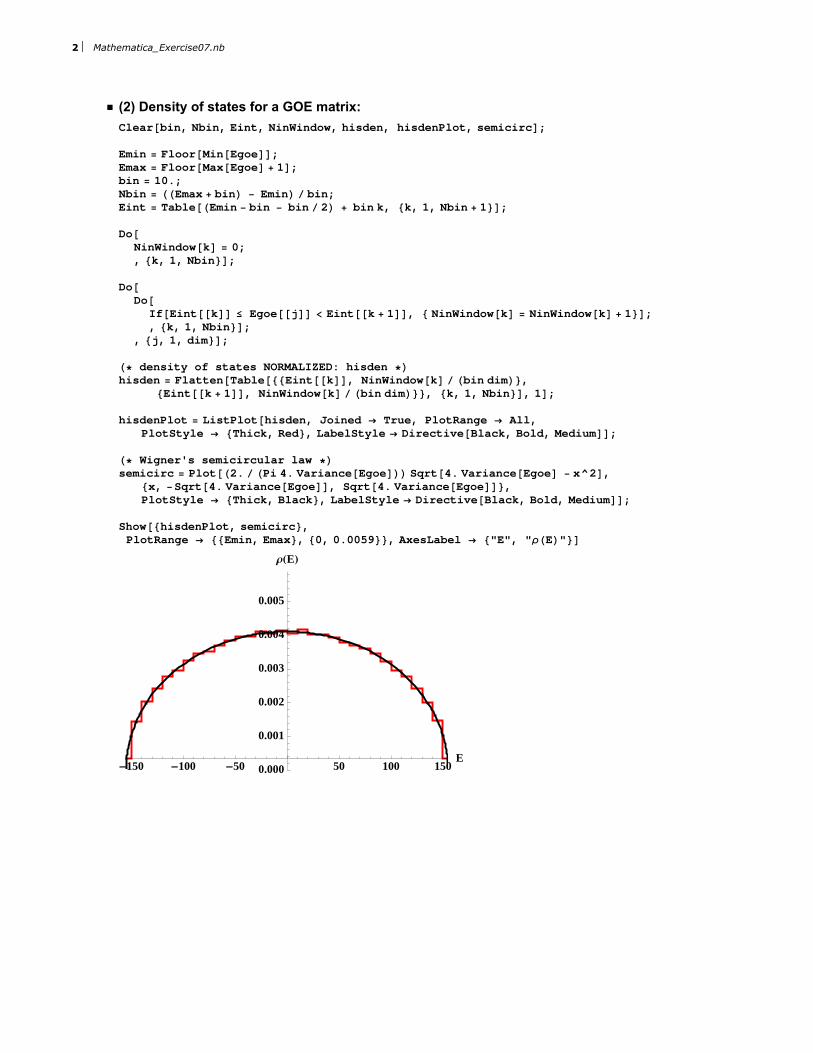
� (3) IPR of each eigenstate vs energy

Clear@IPRgoe, tabIPRD;Do@

IPRgoe@jD = 1 � Sum@Abs@Vecgoe@@j, kDD D^4, 8k, 1, dim<D;, 8j, 1, dim<D;

tabIPR = Table@8Egoe@@jDD, IPRgoe@jD<, 8j, 1, dim<D;

ListPlot@tabIPR, PlotRange ® 80, dim � 2 - 10<, PlotStyle ® Red,LabelStyle ® Directive@Black, Bold, MediumD, AxesLabel ® 8"E", "IPR"<D

-150 -100 -50 0 50 100 150E

200

400

600

800

1000

1200

1400

NPC

Mathematica_Exercise07.nb 3

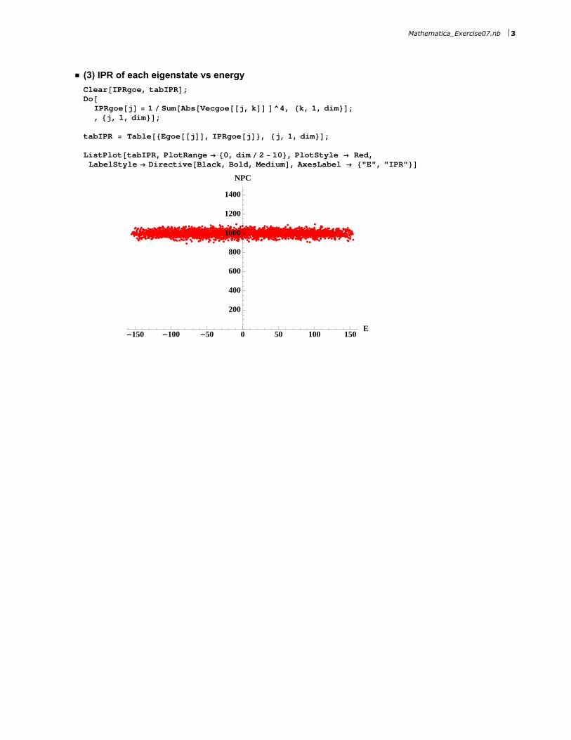
H* H4L LEVEL SPACINGS OF THE UNFOLDED SPECTRUM *LH* Order the eigenvalues from lowest to highest values *LClear@EnerD;Ener = Sort@Table@Egoe@@kDD, 8k, 1, dim<DD;

H* Discard ~10% of the eigenvalues located at the borders of the spectrum *LClear@percentage, half, spacingD;percentage = 0.1 dim;half = Floor@percentage � 2.D;Do@

Clear@averageD;H* Compute the neighboring level spacings

for the remaining eigenvalues after unfolding them *LH* Unfolding here means that the average of each group of 10 level spacings = 1 *Laverage = HEner@@half + 10 jDD - Ener@@half + 10 Hj - 1LDDL � 10.;Do@spacing@iD = HEner@@half + iDD - Ener@@Hhalf - 1L + iDDL � average;

, 8i, 1 + 10 Hj - 1L, 10 j<D;, 8j, 1, Floor@Hdim - percentageL � 10D<D;

H* HISTOGRAM *LClear@spcmin, spcmax, bin, NofbinsD;spcmin = 0.;spcmax = 8.;bin = 0.1;Nofbins = IntegerPart@Hspcmax - spcminL � binD;

Clear@SPChist, NhistD;SPChist@1D = spcmin;Do@SPChist@i + 1D = SPChist@iD + bin, 8i, 1, Nofbins<D;Do@Nhist@jD = 0., 8j, 1, Nofbins<D;

H* Nhist@jD gives how many spacings wehave in the interval SPChist@j+1D and SPChist@jD *L

Do@Do@

If@SPChist@jD £ spacing@kD < SPChist@j + 1D, Nhist@jD = Nhist@jD + 1D;, 8j, 1, Nofbins<D;

, 8k, 1, 10 Floor@Hdim - percentageL � 10D<D;

H* Normalization *LClear@NormaD;Norma = Sum@bin Nhist@jD, 8j, 1, Nofbins<D;Do@Nhist@jD = Nhist@jD � Norma, 8j, 1, Nofbins<D;

H* ListPlot with the obtained data *LClear@jj, nlD;jj = 0;nl = 8<;Do@jj += 1;

nl = Append@nl, 8SPChist@jjD, Nhist@jjD<D;nl = Append@nl, 8SPChist@jj + 1D, Nhist@jjD<D;, 8j, 1, Nofbins - 1<D;

DataPlot =

ListPlot@nl, Joined ® True, PlotRange ® 880, 8<, 80, 1<<, PlotStyle ® 8Black, Thick<,LabelStyle ® Directive@Black, Bold, MediumD, AxesLabel ® 8"s", "P"<D;

H* Theoretical curves *LWignerDyson =

Plot@Pi s � 2. Exp@-Pi s^2 � 4.D, 8s, 0, 8<, PlotRange ® 80, 1<, PlotStyle ® 8Red, Thick<,LabelStyle ® Directive@Black, Bold, MediumD, AxesLabel ® 8"s", "P"<D;

Poisson = Plot@Exp@-sD, 8s, 0, 8<, PlotRange ® 80, 1<, PlotStyle ® 8Blue, Thick<,LabelStyle ® Directive@Black, Bold, MediumD, AxesLabel ® 8"s", "P"<D;

H* The three curves together *LShow@8DataPlot, WignerDyson, Poisson<, PlotRange ® 880, 4<, 80, 1.1<<D

4 Mathematica_Exercise07.nb

1 2 3 4s

0.2

0.4

0.6

0.8

1.0

P

Mathematica_Exercise07.nb 5