Embed Size (px)
Citation preview

Formalising and Reasoning about Fudgets
by Colin J. Taylor
Technical Report NOTTCS-TR-98-4
Thesis submitted to the University of Nottingham
for the degree of Doctor of Philosophy
December 1998

Contents
Abstract v
Acknowledgements vi
1 Introduction 1
1.1 Functional programming . . . . . . . . . . . . . . . . . . . . . . . . 2
1.2 Reasoning about functional programs . . . . . . . . . . . . . . . . . 3
1.3 Reasoning about Fudget programs . . . . . . . . . . . . . . . . . . . 4
1.4 Results . . . . . . . . . . . . . . . . . . . . . . . . . . . . . . . . . . 5
1.5 Dissertation outline . . . . . . . . . . . . . . . . . . . . . . . . . . . 6
2 Background 8
2.1 I/O in functional programming languages . . . . . . . . . . . . . . . 9
2.1.1 Streams . . . . . . . . . . . . . . . . . . . . . . . . . . . . . 10
2.1.2 Continuation passing I/O . . . . . . . . . . . . . . . . . . . 11
2.1.3 Monads . . . . . . . . . . . . . . . . . . . . . . . . . . . . . 12
2.1.4 Uniqueness types . . . . . . . . . . . . . . . . . . . . . . . . 13
2.1.5 Semantics of functional I/O . . . . . . . . . . . . . . . . . . 13
2.2 Graphical development systems . . . . . . . . . . . . . . . . . . . . 14
2.2.1 Haggis . . . . . . . . . . . . . . . . . . . . . . . . . . . . . . 14
2.2.2 Tk-Gofer . . . . . . . . . . . . . . . . . . . . . . . . . . . . . 15
i

2.2.3 eXene . . . . . . . . . . . . . . . . . . . . . . . . . . . . . . 16
2.2.4 Clean . . . . . . . . . . . . . . . . . . . . . . . . . . . . . . 17
2.2.5 Pidgets . . . . . . . . . . . . . . . . . . . . . . . . . . . . . . 17
2.2.6 Fran . . . . . . . . . . . . . . . . . . . . . . . . . . . . . . . 18
2.3 Concurrency . . . . . . . . . . . . . . . . . . . . . . . . . . . . . . . 19
3 Fudgets 21
3.1 Stream processors . . . . . . . . . . . . . . . . . . . . . . . . . . . . 22
3.1.1 Examples . . . . . . . . . . . . . . . . . . . . . . . . . . . . 23
3.1.2 Stateful stream processors . . . . . . . . . . . . . . . . . . . 24
3.1.3 Combinators . . . . . . . . . . . . . . . . . . . . . . . . . . . 25
3.1.4 Primes using stream processors . . . . . . . . . . . . . . . . 26
3.2 Fudgets . . . . . . . . . . . . . . . . . . . . . . . . . . . . . . . . . 27
3.2.1 Layout . . . . . . . . . . . . . . . . . . . . . . . . . . . . . . 28
3.2.2 The counter program . . . . . . . . . . . . . . . . . . . . . . 29
3.2.3 Higher-order fudgets . . . . . . . . . . . . . . . . . . . . . . 30
3.3 Fudget implementations . . . . . . . . . . . . . . . . . . . . . . . . 31
3.3.1 Chalmers Fudgets . . . . . . . . . . . . . . . . . . . . . . . . 31
3.3.2 Budgets . . . . . . . . . . . . . . . . . . . . . . . . . . . . . 32
3.3.3 Fudgets in Tk-Gofer . . . . . . . . . . . . . . . . . . . . . . 33
3.3.4 Embracing Windows . . . . . . . . . . . . . . . . . . . . . . 34
3.3.5 Fudgets in Gadgets . . . . . . . . . . . . . . . . . . . . . . . 34
3.3.6 Concurrent Haskell Fudgets . . . . . . . . . . . . . . . . . . 35
4 Core Fudgets 36
4.1 Types . . . . . . . . . . . . . . . . . . . . . . . . . . . . . . . . . . 36
4.2 Terms . . . . . . . . . . . . . . . . . . . . . . . . . . . . . . . . . . 37
4.2.1 Examples . . . . . . . . . . . . . . . . . . . . . . . . . . . . 40
4.3 Encoding fudgets in Core Fudgets . . . . . . . . . . . . . . . . . . . 42
ii

5 The �-calculus 47
5.1 Overview . . . . . . . . . . . . . . . . . . . . . . . . . . . . . . . . . 48
5.2 Syntax . . . . . . . . . . . . . . . . . . . . . . . . . . . . . . . . . . 49
5.3 Types . . . . . . . . . . . . . . . . . . . . . . . . . . . . . . . . . . 51
5.4 Semantics . . . . . . . . . . . . . . . . . . . . . . . . . . . . . . . . 54
5.4.1 Recursive process de�nitions . . . . . . . . . . . . . . . . . . 58
6 Denotational semantics of Core Fudgets 59
6.1 Denotational semantics . . . . . . . . . . . . . . . . . . . . . . . . . 60
6.2 A �-calculus semantics . . . . . . . . . . . . . . . . . . . . . . . . . 60
6.3 A �-calculus semantics of literals . . . . . . . . . . . . . . . . . . . 61
6.4 A �-calculus semantics of the �-calculus . . . . . . . . . . . . . . . 63
6.4.1 An Example . . . . . . . . . . . . . . . . . . . . . . . . . . . 65
6.5 A �-calculus semantics of stream processors . . . . . . . . . . . . . 66
6.5.1 Lists . . . . . . . . . . . . . . . . . . . . . . . . . . . . . . . 67
6.5.2 Unbounded bu�ers . . . . . . . . . . . . . . . . . . . . . . . 69
6.5.3 Atomic stream processors . . . . . . . . . . . . . . . . . . . 70
6.5.4 Composite stream processors . . . . . . . . . . . . . . . . . . 71
7 Reasoning about Core Fudgets 76
7.1 Bisimulation for the �-calculus . . . . . . . . . . . . . . . . . . . . . 76
7.1.1 Weak bisimulations . . . . . . . . . . . . . . . . . . . . . . . 83
7.1.2 Equivalence for Core Fudgets . . . . . . . . . . . . . . . . . 84
7.2 Examples . . . . . . . . . . . . . . . . . . . . . . . . . . . . . . . . 85
7.2.1 The identity stream processor . . . . . . . . . . . . . . . . . 85
7.2.2 Commutativity of parallel composition . . . . . . . . . . . . 87
7.3 Analysis of �-calculus encoding . . . . . . . . . . . . . . . . . . . . 89
7.4 Semantic issues . . . . . . . . . . . . . . . . . . . . . . . . . . . . . 90
iii

8 Operational semantics of Core Fudgets 92
8.1 An Operational semantics . . . . . . . . . . . . . . . . . . . . . . . 93
8.1.1 Feed . . . . . . . . . . . . . . . . . . . . . . . . . . . . . . . 93
8.1.2 Actions . . . . . . . . . . . . . . . . . . . . . . . . . . . . . 94
8.1.3 Transitions . . . . . . . . . . . . . . . . . . . . . . . . . . . 95
8.1.4 Examples . . . . . . . . . . . . . . . . . . . . . . . . . . . . 102
8.2 A semantic theory . . . . . . . . . . . . . . . . . . . . . . . . . . . 104
8.2.1 First-order bisimulation . . . . . . . . . . . . . . . . . . . . 106
8.2.2 Higher-order bisimulation . . . . . . . . . . . . . . . . . . . 108
8.2.3 Examples . . . . . . . . . . . . . . . . . . . . . . . . . . . . 111
9 Axioms and applications 113
9.1 Axioms . . . . . . . . . . . . . . . . . . . . . . . . . . . . . . . . . . 113
9.2 Correctness of implementations . . . . . . . . . . . . . . . . . . . . 118
10 Summary and further work 135
10.1 Further work . . . . . . . . . . . . . . . . . . . . . . . . . . . . . . 136
A Proof of theorem 8.1 138
A.1 Overview of the proof . . . . . . . . . . . . . . . . . . . . . . . . . . 138
A.2 Compatible re�nement . . . . . . . . . . . . . . . . . . . . . . . . . 139
A.3 Compatible closure . . . . . . . . . . . . . . . . . . . . . . . . . . . 142
A.4 Congruence of � . . . . . . . . . . . . . . . . . . . . . . . . . . . . 144
References 163
iv

Abstract
The Fudgets system is a toolkit for developing graphical applications in the func-
tional language Haskell. It models graphical objects by processes, which can be
combined using a set of combinators. Although numerous programs have been
developed using the Fudgets system, there has been little work upon formally
reasoning about these programs. This dissertation identi�es a core language un-
derlying the Fudgets system, which we call Core Fudgets. Two separate semantic
theories are developed for reasoning about programs written in this core langauge.
We begin by developing a denotational semantics, which considers the meaning
of Core Fudget programs as �-calculus processes. We investigate the use of the
theory of the �-calculus to reason indirectly about Core Fudget programs. Al-
though this works in theory, it turns out to be awkward in practice. This can be
seen as a consequence of the low-level nature of the �-calculus in comparison to
the Core Fudgets language.
Using the insights gained from constructing the denotational semantics we de-
velop an operational semantics for Core Fudgets, which considers programs as
operational transitions. We develop a corresponding semantic theory based upon
the concept of bisimulation, and show the associated equivalence to be a congru-
ence. We use this theory to prove a set of equational rules useful for reasoning
about Core Fudget programs. Finally, we de�ne a notion of implementation cor-
rectness with respect to our operational semantics, and illustrate it by analysing a
speci�c implementation.
The Core Fudgets language abstracts away from the graphical details of the
Fudgets system and concentrates on the underlying communication and compu-
tation mechanisms. The theory we develop forms a foundation upon which these
graphical details may be examined formally.
v

Acknowledgements
Firstly, my thanks go to the Languages and Programming research group in the
Computer Science Department at the University of Nottingham for the facilities
they have provided for my use. I would like to express my gratitude to Graham
Hutton and Mark P. Jones as my supervisors for their encouragement, excellent
guidance and providing me with the chance to study at Nottingham. I am also
delighted to acknowledge the support of the University of Nottingham, without
whose funding this research work would not have been possible.
Many thanks also to my friends in `Lapland' for making my time studying in
Nottingham a pleasurable and pro�table experience. Special thanks must go to
Benedict R. Gaster, Claus Reinke and Louise Dennis for the many discussions we
had, and also to Anthony C. Daniels for proof-reading and for listening to my
jokes.
Outside of Nottingham, my colleagues in the programming language research
community have inspired and challenged me. In particular, this dissertation would
not be possible without the Fudgets system developed by Thomas Hallgren and
Magnus Carlsson. I thank the many people with whom I had discussions including
Rob Noble, Sigbj�rn Finne, Colin Runciman and Simon Peyton Jones.
Finally, I would like to thank my parents for their continued support and belief
in my aims even when I was unsure of them myself.
vi

List of Figures
3.1 Sieve of Eratosthenes . . . . . . . . . . . . . . . . . . . . . . . . . . 26
3.2 A Fudget . . . . . . . . . . . . . . . . . . . . . . . . . . . . . . . . 27
3.3 The counter program . . . . . . . . . . . . . . . . . . . . . . . . . . 29
3.4 Higher-order fudgets in action . . . . . . . . . . . . . . . . . . . . . 30
3.5 A Higher-order Fudget program . . . . . . . . . . . . . . . . . . . . 31
4.1 Type rules for literals . . . . . . . . . . . . . . . . . . . . . . . . . . 39
4.2 Type rules for expressions . . . . . . . . . . . . . . . . . . . . . . . 40
4.3 Type rules for stream processors . . . . . . . . . . . . . . . . . . . . 41
4.4 Type rules for constant functions . . . . . . . . . . . . . . . . . . . 42
4.5 Serial composition for fudgets, A >==<F B . . . . . . . . . . . . . 44
4.6 Encoding serial composition . . . . . . . . . . . . . . . . . . . . . . 44
4.7 Encoding parallel composition . . . . . . . . . . . . . . . . . . . . . 45
4.8 Feedback for fudgets, LoopF A . . . . . . . . . . . . . . . . . . . . 45
4.9 Encoding of feedback . . . . . . . . . . . . . . . . . . . . . . . . . . 46
5.1 Type rules for values . . . . . . . . . . . . . . . . . . . . . . . . . . 52
5.2 Type rules for processes . . . . . . . . . . . . . . . . . . . . . . . . 53
5.3 An example typing derivation . . . . . . . . . . . . . . . . . . . . . 54
5.4 Free and bound variables . . . . . . . . . . . . . . . . . . . . . . . . 55
5.5 Semantics for the �-calculus . . . . . . . . . . . . . . . . . . . . . . 56
vii

6.1 Denotational semantics for Core Fudgets . . . . . . . . . . . . . . . 59
6.2 An encoding of booleans . . . . . . . . . . . . . . . . . . . . . . . . 61
6.3 An encoding of natural numbers . . . . . . . . . . . . . . . . . . . . 62
6.4 An encoding of binary sums . . . . . . . . . . . . . . . . . . . . . . 63
6.5 An encoding of the �-calculus . . . . . . . . . . . . . . . . . . . . . 64
6.6 An encoding of type contexts . . . . . . . . . . . . . . . . . . . . . 65
6.7 An encoding of lists . . . . . . . . . . . . . . . . . . . . . . . . . . . 67
6.8 Reversing lists . . . . . . . . . . . . . . . . . . . . . . . . . . . . . . 68
6.9 A typing derivation for Nil . . . . . . . . . . . . . . . . . . . . . . . 68
6.10 Bu�ers . . . . . . . . . . . . . . . . . . . . . . . . . . . . . . . . . . 69
6.11 An encoding of stream processor types . . . . . . . . . . . . . . . . 70
6.12 An encoding of atomic stream processors . . . . . . . . . . . . . . . 71
6.13 An encoding of serial composition . . . . . . . . . . . . . . . . . . . 71
6.14 An encoding of parallel composition . . . . . . . . . . . . . . . . . . 72
6.15 Splitting of streams . . . . . . . . . . . . . . . . . . . . . . . . . . . 72
6.16 An encoding of feedback . . . . . . . . . . . . . . . . . . . . . . . . 73
6.17 An encoding of dynamic stream processors . . . . . . . . . . . . . . 74
7.1 An early transition semantics . . . . . . . . . . . . . . . . . . . . . 79
7.2 A late transition semantics . . . . . . . . . . . . . . . . . . . . . . . 80
8.1 The relationship between the semantics . . . . . . . . . . . . . . . . 92
8.2 The duality of PutSP and � . . . . . . . . . . . . . . . . . . . . . 94
8.3 Type rule for feed . . . . . . . . . . . . . . . . . . . . . . . . . . . . 94
8.4 Type rules for actions . . . . . . . . . . . . . . . . . . . . . . . . . . 95
8.5 An output example . . . . . . . . . . . . . . . . . . . . . . . . . . . 102
8.6 The discard example . . . . . . . . . . . . . . . . . . . . . . . . . . 103
8.7 The semantics of the identity stream processor . . . . . . . . . . . . 103
viii
8.8 A mixed input and output example . . . . . . . . . . . . . . . . . . 103
8.9 An example of terms not �1 equivalent . . . . . . . . . . . . . . . . 107
8.10 Action extension rules . . . . . . . . . . . . . . . . . . . . . . . . . 108
8.11 The relationship between the bisimulation equivalences . . . . . . . 111
9.1 A representation of stream processors . . . . . . . . . . . . . . . . . 120
9.2 Atomic transitions . . . . . . . . . . . . . . . . . . . . . . . . . . . 121
9.3 The implementation of serial composition . . . . . . . . . . . . . . . 121
9.4 Transition rules for serial composition . . . . . . . . . . . . . . . . . 122
9.5 Parallel composition . . . . . . . . . . . . . . . . . . . . . . . . . . 123
9.6 Transition rules for parallel composition . . . . . . . . . . . . . . . 124
9.7 The implementation of feed . . . . . . . . . . . . . . . . . . . . . . 125
9.8 Transition rules for feed . . . . . . . . . . . . . . . . . . . . . . . . 125
9.9 The implementation of feedback . . . . . . . . . . . . . . . . . . . . 126
9.10 Transition rules for feedback . . . . . . . . . . . . . . . . . . . . . . 126
9.11 The implementation of dynamic stream processors . . . . . . . . . . 126
9.12 Transition rules for dynamic stream processors . . . . . . . . . . . . 127
9.13 The modi�ed implementation of serial composition . . . . . . . . . 129
9.14 New serial composition transition rules . . . . . . . . . . . . . . . . 129
A.1 Compatible re�nement for literals and expressions . . . . . . . . . . 139
A.2 Compatible re�nement for stream processors . . . . . . . . . . . . . 140
A.3 Compatible re�nement for constant functions . . . . . . . . . . . . . 141
A.4 Properties of compatible closure . . . . . . . . . . . . . . . . . . . . 142
A.5 Transitive re exive closure . . . . . . . . . . . . . . . . . . . . . . . 160
ix

Chapter 1
Introduction
Numerous toolkits have been developed to construct functional programs with
graphical interfaces. One particular toolkit is the Fudgets system [CH98] for the
functional programming language Haskell, which models graphical objects by pro-
cesses that can be combined using a simple set of combinators. Although many
graphical programs have been developed using this system, there has been little
work on formally reasoning about such programs. This dissertation shows that we
can reason about programs written in the Fudgets system, and that this is useful
for both the programmer using the system and the implementer of the system. We
develop two separate theories for the Fudgets system, both of which are inspired
by ideas from concurrency theory.
The �rst semantics we develop associates meanings to Fudget programs by a
translation into the �-calculus [MPW89]. This allows us to make use of the existing
theory of the �-calculus to reason about Fudget programs. Although this works in
theory, it turns out to be awkward in practice. This provides the motivation for
the second semantics that we develop. This second semantics associates meanings
to Fudget programs by operational transitions, resulting in a more direct seman-
tics. A corresponding theory is developed for this semantics based on the idea of
bisimulation [Par81] from concurrency theory.
We examine two applications of semantic theories for the Fudgets system.
Firstly, we develop some equational rules, from the theories, that can be used
to reason directly about Fudget programs. Secondly, we de�ne what it means for
an implementation to be correct with respect to the theories, and we examine a
speci�c implementation to illustrate this.
1

Chapter 1. Introduction 2
1.1 Functional programming
Functional or applicative programming languages place an emphasis on the evalu-
ation of expressions instead of on the execution of commands. Expressions in these
languages are constructed from basic values which are combined using functions.
Church's �-calculus [Chu41] is the prototypical functional programming lan-
guage. However, this was developed with the motivation of creating a calculus
capturing the intuitive behaviour of functions, and was not thought of as a pro-
gramming language at the time. Church's �-notation for anonymous functions was
adopted by McCarthy in the Lisp programming language [McC60] which is one of
the earliest real functional languages. The next signi�cant step in functional pro-
gramming came in the ISWIM family of languages introduced by Landin [Lan66].
He introduced a number of innovations including an emphasis towards equational
reasoning | reasoning about programs by replacing expressions with other equal
expressions.
There are numerous modern functional languages such as Haskell [PH96], Mi-
randa [Tur85], SML [MTH90], Lisp [McC60], and Clean [NSvEP91]. An important
property of these languages is the semantics they attribute to function application.
The two main ways in which function application can be interpreted are referred to
as call-by-value semantics, and call-by-name semantics. In call-by-value semantics,
the argument to a function is completely evaluated before the function is called.
Alternatively, call-by-name semantics does not evaluate the argument before call-
ing the function, instead when the function requires the value of the argument it
is evaluated and this may occur multiple times. An eager functional language is
one that has call-by-value semantics, whereas a lazy functional language has call-
by-name semantics. In practice, function application in lazy languages is usually
implemented with a call-by-need semantics which is the same as call-by-name ex-
cept once an argument has been evaluated its value is stored to be recalled when
the argument is next demanded. Haskell, Miranda and Clean are lazy functional
languages, while Lisp and SML are eager.
In this dissertation we consider the Fudgets system which is implemented in
Haskell. The concepts at the heart of this system are not restricted just to Haskell,
and in our formal treatment of this system we will consider call-by-name semantics
for function application. However, we believe it would be possible to modify our
results for other function application semantics, such as call-by-value.

Chapter 1. Introduction 3
1.2 Reasoning about functional programs
An often stated advantage of functional programs is the ease with which one can
reason about them. Reasoning about programs can be used to show that a pro-
gram meets a speci�cation, and also to optimise performance, space usage or other
characteristics. There are many techniques available to the functional program-
mer to prove properties of their programs. In this section we review some of these
methods including equational reasoning, induction, and coinduction.
Properties of functional programs are often proven by using equational rea-
soning, where an expression can be replaced by another that has an equal value
without altering the overall meaning of the program. This technique is not just
applicable to functional languages but it is usually much easier to demonstrate
two expressions to have equal values for such languages. This is because most
functional languages are pure, meaning that the value of a function depends only
on the values of its arguments. A simple example of equational reasoning allows
us to rewrite the integer doubling function as follows:
double x = x + x (De�nition of double)
= 2 � x (Arithmetic)
In this case, the resulting function might be more e�cient than the original. Dar-
lington and Burstall's classic work [BD77] on equational reasoning advocates an
unfold/fold approach. A program is symbolically evaluated { unfolded { and then
the resulting program is rearranged and recursion introduced { folded.
An important idea in functional programming is the recursive de�nition of func-
tions. Properties can be proven of such functions by using mathematical induction
on the structure of the function arguments, which in the case the arguments are
of base types, such as numbers, corresponds to normal mathematical induction.
Another technique that is more suitable for proving properties of functions
manipulating in�nite data structures is coinduction { the dual proof principle
to induction. Gordon [Gor92] advocates an operational approach to functional
programming based on concurrency theory. In this approach, equivalence of terms
can be de�ned using the concept of bisimulation [Par81] which admits coinductive
proofs [MT90, Pit94]. Input and output can be integrated into this approach
allowing interactive functional programs to be reasoned about.

Chapter 1. Introduction 4
1.3 Reasoning about Fudget programs
The Fudgets system is a toolkit for developing graphical applications in the func-
tional language Haskell. It models graphical objects by simple processes, which
can be combined using a simple set of combinators. Although many programs have
been developed using the Fudgets system, there has been little work on formally
reasoning about these programs. The primary goal of this dissertation is to explain
the semantics of the Fudgets system, enabling properties to be proven of Fudget
programs. There are two other attempts to de�ne such a semantics that we are
aware of:
A demand driven operational semantics for Fudgets: Hallgren and Carls-
son [HC95] describe a simple operational semantics for the Fudgets system using
rewriting rules. This semantics takes a demand driven approach, reducing the
graphical objects in a Fudgets program that produce output before those that
require input. Nondeterministic rewriting rules capture the concurrency of com-
posing these graphical objects in parallel. The approach we take in this dissertation
is inspired by concurrency theory and has no bias towards generating output over
consuming input. The resulting semantics that we describe has more scope for
concurrency and includes Hallgren and Carlsson's semantics as an instance.
A calculus for stream processors: More recently, Hallgren and Carlsson [CH98]
have suggested a calculus for stream processors | the central concept in the Fud-
gets system. The calculus they propose is similar to the semantics we develop in
this dissertation. However, their calculus is untyped and although they de�ne an
equivalence based on bisimulation they do not show it to be a congruence. They
also show how the �-calculus can be encoded in their stream processor calculus,
but this requires streams to be able to carry values of di�erent types, which con-
tradicts one of the design principles of the Fudgets system. This is not a problem
for their untyped calculus but as a result we cannot use their encoding with the
semantics we consider in this dissertation.
This dissertation develops two theories of the Fudgets system. The �rst is
based on a denotational semantics using the �-calculus, which provides a founda-
tion for investigating some of the semantic issues in the Fudgets system. However,

Chapter 1. Introduction 5
this theory is complicated to use to prove properties of Fudget programs. Conse-
quently, we develop a more practical theory based on Gordon's operational theory
of functional languages, which makes reasoning about Fudget programs simpler.
We only concern ourselves with the logical behaviour of Fudget programs in this
dissertation. Two Fudget programs that have the same logical behaviour but that
di�er in their physical appearance will be considered to be equivalent programs.
1.4 Results
The main contribution of this dissertation is to formalise the Fudgets system and
to show how properties can be proven of programs written in the Fudgets system.
The following list indicates speci�c original results:
� Identi�cation of a core language of the Fudgets system.
� A denotational theory of the Core Fudgets language, based on a translation
into the �-calculus.
� An investigation into using the denotational semantics for reasoning about
Core Fudget programs.
� An operational theory of the Core Fudgets language, based on ideas from
concurrency theory.
� An investigation into suitable equivalences for the operational theory, and a
proof of congruence for the �nal equivalence we consider.
� A set of equational rules correct with respect to the operational semantics
which are useful for reasoning about Core Fudget programs.
� A de�nition of implementation correctness with respect to the operational
semantics, and an investigation into the correctness of the original Fudgets
implementation.

Chapter 1. Introduction 6
1.5 Dissertation outline
This dissertation can naturally be broken into three parts. The �rst part surveys
related work and introduces the Fudgets system:
Chapter 2: Background. This chapter introduces some useful background ma-
terial for the rest of the dissertation. It begins by describing the problem
of integrating input and output into functional programming languages, and
reviews some of the solutions that have been proposed. The chapter con-
cludes with a survey of some systems, other than the Fudgets system, for
developing graphical applications in functional languages. In particular, we
focus on the semantics of these systems where they exist.
Chapter 3: Fudgets. Fudgets is a system for developing graphical applications
in the functional programming language Haskell. This chapter introduces
the system and reviews some of the implementations of the system.
Chapter 4: Core Fudgets. We introduce the Core Fudgets language, which en-
capsulates the essence of the Fudgets system. This chapter de�nes the syntax,
and type assignment relation for the Core Fudgets language, which forms the
basis for theories of the Fudgets system that we consider in the later chapters.
The second part develops a formal semantics for the Core Fudgets language using
the �-calculus, and uses this to reason about some Core Fudget programs:
Chapter 5: The �-calculus. The �-calculus is a process calculus designed for
modelling mobile processes. This chapter de�nes the syntax, type assignment
relation, and operational semantics of a minor variant of Milner, Parrow, and
Walker's original calculus [MPW89]. This calculus forms the basis of the
semantics examined in Chapter 6.
Chapter 6: Denotational semantics of Core Fudgets. We de�ne a denota-
tional semantics for the Core Fudgets language by translating terms into the
�-calculus of Chapter 5.
Chapter 7: Reasoning about Core Fudgets. We present an overview of the
theory of the �-calculus and then use this to reason about Core Fudget
programs. The chapter concludes with a discussion of the relative advantages

Chapter 1. Introduction 7
and disadvantages of de�ning the semantics of Core Fudgets in terms of the
�-calculus.
The third and �nal part develops an operational semantics for Core Fudgets and a
corresponding equational theory. This theory is used to develop a set of equational
rules and also to investigate the correctness of implementations of Core Fudgets:
Chapter 8: Operational semantics of Core Fudgets. In this chapter we de-
velop an operational semantics for Core Fudgets. We investigate a number
of equivalences for this semantics based upon bisimulation. The �nal equiv-
alence we examine is shown to be a congruence and is used as the basis of
an equational theory for Core Fudgets.
Chapter 9: Axioms and applications We explore the properties of the oper-
ational semantics developed in Chapter 8, and develop a set of equational
rules for Core Fudgets. Some intuitively correct equational rules turn out to
be invalid according to the equational theory of the operational semantics.
We discuss some of these rules and the reasons for why they are invalid in
our model. The operational semantics is also useful for checking the cor-
rectness of implementations of Core Fudgets and we conclude the chapter by
describing how this can be done, illustrating it with the original Chalmers
implementation of Fudgets.
Chapter 10: Summary and further work We end the dissertation by draw-
ing conclusions and with suggestions for further work.

Chapter 2
Background
This chapter introduces some useful background material for the rest of the disser-
tation. First, we consider the problem of extending functional programming lan-
guages with support for input and output. Next, we review some of the systems,
other than the Fudgets system, for developing graphical applications in functional
programming languages. The chapter concludes with a presentation of methods
for extending functional programming languages with concurrent features. This is
useful as most of the systems for developing graphical applications in functional
programming languages, including the Fudgets system, make use of concurrency.
Section 2.1 begins by describing the most obvious method for adding input
and output to a functional programming language. Next we discuss the problems
associated with this method, and the section concludes by reviewing the most
widely used solutions to these problems. Section 2.2 reviews a number of systems
other than the Fudgets system for developing graphical applications in functional
programming languages. Speci�cally, we concentrate on systems using the lazy
functional programming language Haskell, and discuss the formal semantics of
these systems where they exist. Finally, the chapter concludes in Section 2.3,
which examines methods for extending functional programming languages with
concurrent constructs.
8

Chapter 2. Background 9
2.1 I/O in functional programming languages
Perhaps the most obvious way to add support for input and output is to use side
e�ecting primitives similar to the functions used in imperative languages such as
C [KR89]. This is by far the most widely used mechanism for I/O in functional
programming languages and can be found in LISP, Scheme and Standard ML. An
example of such side e�ecting primitives in Haskell might look like:
getChar :: Char
putChar :: Char ! ()
The getChar function waits for a key to be pressed and returns the corresponding
character, while putChar c prints the character speci�ed by its argument c.
Although such side e�ecting primitives seem to provide a direct method for
adding I/O to a functional language they do not combine well with lazy functional
programming languages. There are several reasons why this is the case; the �rst
is that to use such primitives a programmer must know the details of the order of
evaluation for the language. Laziness makes this more di�cult to predict than for
eager functional programming languages.
Normally, in a functional programming language terms either diverge or con-
verge to some canonical value. However, in the presence of side e�ecting primitives
this is no longer the case, because a term may perform some I/O operation and
then continue as another term. This complicates reasoning about programs as
there are more cases to consider when proving properties of terms. This applies
for both eager and lazy functional programming languages
Finally, lazy functional programming languages with side e�ecting primitives
have di�erent call-by-name and call-by-need semantics. A simple example illus-
trates the problem:
(nx ! x == x ) getChar
Under call-by-name semantics two characters are read, whereas only one is read
under call-by-need. This is important as call-by-name is usually implemented with
a call-by-need semantics, but this is unsound if side e�ecting primitives are present
in the language.

Chapter 2. Background 10
A number of approaches have been proposed for solving these problems of
adding input and output to functional programming languages. In the following
sections we review the most common of these approaches.
2.1.1 Streams
A stream is a lazy list of data objects. Miranda1 [Tur85], Ponder [Fai85] and Hope
[BMS80] use streams for I/O. In these systems, an interactive program is modelled
as a function from one stream representing the input, to another representing the
output. This is referred to as Landin-stream I/O, and if we consider simple teletype
I/O then a program is a function mapping a stream of input characters to a stream
of output characters. For example, in Haskell we might use lists to model streams,
and then a program converting all its input to uppercase is written as follows:
uppercase :: [Char ]! [Char ]
uppercase inp = map toUpper inp
The function toUpper is a part of the standard Haskell prelude and maps a char-
acter to its uppercase equivalent. The streams used for I/O must be lazy to allow
output to be interleaved with reading input, otherwise all of the user's input would
have to be read before any output could be produced.
There is another form of stream I/O, called synchronised-stream I/O, which
is a generalised form of Landin-stream I/O. A synchronised-stream program is a
function mapping a stream of I/O acknowledgements to a stream of I/O requests.
Each request is synchronised by an acknowledgement. For example, if we de�ne
the I/O requests and acknowledgements by the datatypes:
data Req = GetChar j PutChar Char
data Ack = ReadChar Char j Ok
then the example converting input to uppercase is written as the program:
uppercase :: [Ack ]! [Req ]
uppercase acks = GetChar : (case acks of ((ReadChar c) : as) !
(PutChar (toUpper c)) : (case as of (Ok : as 0) !
uppercase as 0))
1Miranda is a trademark of Research Software Ltd.

Chapter 2. Background 11
In Landin-stream I/O output is produced whenever the next value in the output
stream is determined, and input occurs whenever it is demanded from the input
stream. However, in synchronised I/O every I/O request is synchronised with a
corresponding I/O acknowledgement. This allows any kind of I/O operation to be
encoded using synchronised-stream I/O.
2.1.2 Continuation passing I/O
Continuation passing I/O was �rst introduced in the functional operating system
Nebula [Kar81]. It uses a datatype to represent the interactive actions of a pro-
gram. Considering simple teletype input and output this datatype might be:
data CPIO = PutChar Char CPIO
j GetChar (Char ! CPIO)
j Done
A value of type PutChar c k represents the I/O action that outputs the char-
acter c and then continues as the program k . The term GetChar f corresponds
to an I/O action that reads an input character c and then continues as the pro-
gram f c. Lastly, the term Done represents a program that has terminated. A
program of type CPIO is executed by a small interpreter acting outside of the
language's normal reduction mechanism. When a program is reduced to the term
PutChar c k then this interpreter actually performs the output action, and then
starts evaluation of the continuation k . Similarly, a program that reduces to the
term GetChar f invokes the interpreter to wait for an input character. Once this
input character, c, is received then evaluation restarts with the term f c. Finally,
when a program reduces to the constructor Done then the interpreter terminates.
Continuation passing I/O works by specifying an exact order of evaluation for
the I/O actions regardless of the calling convention of the underlying functional
programming language [Plo75]. As a result they can be used in both eager and
lazy functional programming languages as the basis of an I/O system. The name
continuation passing I/O stems from the arguments k and f in the PutChar and
GetChar constructs, which act as continuations in a style similar to the continua-
tions used in denotational semantics [SW74].
Chapter 2. Background 12
2.1.3 Monads
Motivated by the work of Moggi [Mog89] and Spivey [Spi90], Wadler [Wad92,
Wad90] proposed a style of functional programming based on monads that can
be used to model impure `features' such as input and output. The type system
is used to distinguish between normal functional values and computations that
may perform side e�ects. For example, a value of the monadic type IO a is a
computation that may perform some side e�ects returning a result of type a. All
side e�ecting functions are embedded into this monadic type:
getChar :: IO Char
putChar :: Char ! IO ()
Normal functional values are embedded into the monadic type using the return
function, whilst values of the monadic type are combined using the function >>=:
return :: a ! IO a
(>>=) :: IO a ! (a ! IO b)! IO b
A program is a value of the monadic type IO (), and a simple example is a program
that converts all input to uppercase, which is written as:
uppercase :: IO ()
uppercase = getChar >>= (nc !
putChar (toUpper c) >>= (n !
uppercase))
When a program is executed, the actions embedded in the monadic type are per-
formed, realising the input and output. It is essential that the monadic type IO a
is an abstract datatype whose de�nition is not visible to the programmer. This en-
sures that values of the monadic type can only be constructed using the primitive
functions such as getChar and the combinators return and >>=. As a result of
this the monadic primitives such as getChar can only be used in a single threaded
manner, and thus it is safe to implement them using side e�ecting functions. This
mechanism is used in Haskell 1.3 [PH96].

Chapter 2. Background 13
2.1.4 Uniqueness types
The Clean language [NSvEP91] includes a linear type system called Uniqueness
Types [SBvEP94] which allow programs to de�ne functions that can perform side
e�ects. If it can be guaranteed that the object on which a side e�ect is being
performed is not used elsewhere then it is safe to update the object in-place. In
Clean the type system is used to express when objects cannot be shared. The pro-
grammer adds a unique annotation to the types of function arguments to indicate
if they must not be shared. The result type of a function can also be annotated
to indicate if no sharing is introduced in the result. This mechanism enforces the
single threaded use of objects. An illustrative example is the type of the function
FWriteC that writes a character to a given �le as a side-e�ect. Its type is:
:: FWriteC CHAR UNQ FILE ! UNQ FILE
and it takes a character and a unique �le as its two arguments, returning a unique
�le as its result. This type speci�cation guarantees that the �le it is passed is not
used elsewhere. An example of a dangerous use of the function is:
:: Dangerous UNQ FILE ! (UNQ FILE ;UNQ FILE );
Dangerous �le ! (FWriteC 0a 0 �le;FWriteC 0b 0 �le);
In the body of the Dangerous function FWriteC is called twice but �le is no
longer a unique �le because it is used twice, and it is therefore rejected by the
typing system.
2.1.5 Semantics of functional I/O
There is a large body of work concerned with input and output in functional
languages. However, very little of this work has addressed the issue of semantics
for input and output. The most comprehensive work on the semantics of input
and output in lazy functional languages is Gordon's dissertation [Gor92], where
he develops an operational semantics and a corresponding equational theory based
on Abramsky's applicative bisimulation [Abr89]. Previous to this, Hudak and
Sundaresh [HS89] examined the expressiveness of purely functional I/O systems,
and Thompson [Tho87] investigated streams in Miranda.

Chapter 2. Background 14
2.2 Graphical development systems
In this section we review some systems for developing graphical applications in
functional languages. We describe the language features the systems make use
of, such as for handling input and output, and the abstractions they support for
constructing graphical applications. The review of each system concludes with an
examination of any semantics that have been developed for the system.
We mainly concern ourselves with systems for the lazy functional programming
language Haskell, and begin by examining the Haggis system and Tk-Gofer which
are both based on Haskell. However, to provide a contrast, we next consider the
eXene graphical development system written in Standard ML, and the graphical
system for the Clean language. Finally, we consider Pidgets and Fran, which
are more suitable for constructing reactive animations than graphical interfaces.
However, it is possible to use them to build such interfaces and we examine them
as representatives of a larger class of systems for reactive programming.
2.2.1 Haggis
The Haggis system [FJ95] provides support for developing graphical applications
in Haskell, and is based on the Concurrent Haskell [FGJ96] extensions for concur-
rent processes. Instead of building a graphical program around a central event-
dispatching loop, a program is modelled as a set of processes which can wait on
semaphores that are set when events occur.
Input and output is handled in Haggis using the IO monad extended with
extra operations for concurrency. Processes can be spawned, and communication
between processes is supported by the use of atomically mutable state. The under-
lying concept in Haggis is the virtual I/O device. Interactive objects are modelled
as virtual I/O devices much like the standard devices in modern operating systems.
Graphical applications are built in Haggis in a compositional style.
Peyton-Jones et. al [FGJ96] describe an operational semantics for Concurrent
Haskell based on ideas from concurrency theory. In their semantics, determinis-
tic computation is separated from the nondeterministic computations that can be
introduced using the concurrency extensions. This allows existing reasoning tech-
niques such as � and � equivalence to be used unmodi�ed for the deterministic
parts of programs.

Chapter 2. Background 15
We are not aware of any formal semantics for the Haggis system in the lit-
erature, but an operational semantics is induced by the semantics for Concurrent
Haskell. This would not result in a particularly abstract semantics but nevertheless
could be used to reason formally about programs in the Haggis system.
2.2.2 Tk-Gofer
The Tk-Gofer GUI library [VSS96] is an extension of the functional language
Gofer [Jon91] and makes use of the Tcl/Tk [Ous94] graphical user interface toolkit.
Input and output is handled in Tk-Gofer using monads which provide a mechanism
for communicating with Tcl/Tk.
Graphical applications are structured using objects called widgets which come in
one of several kinds: toplevel widgets, window widgets, menu widgets, and canvas
widgets. A toplevel widget acts as a container for other widgets, whilst a window
widget is a graphical object such as a button. Menu widgets correspond to pull-
down or pop-up menus, and canvas widgets correspond to objects such as circles
or rectangles that can be placed on a canvas. Each widget has a unique identifying
handle through which it can be manipulated. Tk-Gofer uses the constructor classes
of Gofer to capture the common characteristics of groups of widgets in a class
hierarchy. Widgets can respond to events by specifying callback functions which
will be invoked when a speci�c event occurs. Claessen et. al[CVM97] discuss
various mechanisms, including using constructor classes, to structure graphical
programs in Tk-Gofer.
Although the original Tk-Gofer system did not support concurrency, version 2.0
of the system includes extensions for concurrency. These extensions are based on
Concurrent Haskell and can be used to structure graphical applications as separate
concurrent processes.
There is no formal semantics for Tk-Gofer, but as it uses only minimal exten-
sions to the Gofer functional programming language then it may be possible to
use standard equational reasoning techniques to prove properties of Tk-Gofer pro-
grams. This is not a very abstract method for reasoning about graphical programs,
and assumes that the concurrency extensions are implemented deterministically.

Chapter 2. Background 16
2.2.3 eXene
The eXene toolkit is used for developing graphical applications in Concurrent
ML [Rep91] | a higher-order concurrent language based on the Standard ML [MTH90]
functional programming language. Concurrency is used for the same reason as in
the Haggis system { to avoid biasing the architecture of the application towards
the user interface.
Input and output is handled in eXene using side e�ecting functions whose or-
der of execution is straightforward to predict because Standard ML is an eager
language. Input is divided into three categories: keyboard, mouse and control.
Typically, each window has a concurrent thread for each of these kinds of input,
and may also have some threads for managing state. Events are distributed based
on the hierarchy of windows, and so a window's thread must route events to its
children. This can almost always be done using a generic router built into eXene.
Graphical components are modelled using widgets, and a program creates a hier-
archy of widgets, with the root corresponding to a top-level window in which the
widgets will be realized. Widgets can be customised in three ways; the �rst is to
parameterise them by attributes such as which font to use, or the function to be
called when a speci�c event occurs. The next form of customisation is simple com-
position of widgets to form new widgets. Finally, a widget can be wrapped inside
a function to alter the widget's behaviour, for example, to �lter certain events such
as mouse clicks and hence modify the widgets behaviour to these events.
There have been two main approaches to giving an operational semantics to
Concurrent ML. The �rst, in the tradition of Standard ML [MTH90, MT91], is
to de�ne unlabelled transitions between programs, and Reppy [Rep92] uses this
approach to give a semantics for Concurrent ML. An alternative approach taken
by Ferriera et. al [FHJ95] uses ideas from concurrency theory. Labelled transitions
between terms are de�ned which support equivalences based on bisimulation.
In a similar manner to the Haggis system, the formal semantics for Concurrent
ML induces a semantics for the eXene system. However, this is not a particu-
larly direct semantics and is most likely to be tedious for reasoning about eXene
programs.

Chapter 2. Background 17
2.2.4 Clean
The Clean language includes support for constructing graphical applications using
its uniqueness types. Input and output is performed on objects such as �les that
are o�ered to the programmer as abstract datatypes. Clean supports four main
types of objects for input and output: the world, the �le system, a �le, and the
event I/O system. The world acts as a container of all of the other objects. The
�le system is an object representing the current state of the �le system, while a
�le is an object corresponding to an individual �le. Finally, the event I/O system
is an object modelling the event queue containing events such as key presses, and
mouse clicks.
Clean supports four kinds of abstract devices which correspond to windows,
menus, dialog boxes, and timers. A graphical program consists of a set of algebraic
datatypes de�ning the devices for the program, along with an initial program
state, and some event handling functions. The Clean system handles events in the
order they occur and searches through the device de�nitions to �nd the function
applicable to the event.
The semantics of the Clean language is based on term graph rewriting sys-
tems [BvEG+87], with function de�nitions corresponding to term graph rewriting
rules. Reasoning about Clean programs thus reduces to reasoning about their
corresponding graphs. As long as uniqueness types are preserved by term graph
rewriting systems then this same method can be used to reason about interactive
Clean programs. Barendsen et. al [BS93] prove such a result for a simple form of
uniqueness typing. However, the uniqueness type system in the latest versions of
Clean contain more advanced features and it is unclear as to whether this result
still holds, if this is the case then interactive programs could be reasoned about by
manipulating their graph forms.
2.2.5 Pidgets
Pidgets [Sch95] is a framework for programming graphical applications in the Gofer
functional programming language. It attempts to unify two concepts which are
normally dealt with separately: pictures and widgets. A widget is a graphical
object that can react to events but has limited shapes, while a picture can be of
arbitrary shape but cannot handle events.
Chapter 2. Background 18
Pidgets uses a monadic approach to deal with input and output, and introduces
a monad which can be used to model objects whose values change over time.
These objects can be arranged in a graph where the edges indicate functional
dependencies representing constraints that must be maintained. A Pidget is itself
a special case of one of these objects, where the value of the object corresponds
to the picture's current appearance. The runtime system of Pidgets is written in
C++ [Str97] and has itself developed into a framework for constructing graphical
applications in C++ as described by Scholz et. al [SB96].
We are not aware of any work on formalising a semantics for the Pidgets system.
However, like Tk-Gofer, Pidgets is implemented in Gofer and so it may be possible
to make use of standard equational reasoning techniques to reason about Pidget
programs. However, once again this approach is not particularly abstract and so
is likely to be di�cult to use in practice.
2.2.6 Fran
Fran [EH97] is a system for developing reactive animations in Haskell. The central
ideas in Fran are behaviours and events. A behaviour is a value that can vary over
time and may change, or react, depending on user input. An event corresponds
to an arbitrarily complex condition that may depend on external events such as
mouse clicks and keyboard presses, or animation parameters like the proximity of
objects. Events also carry information such as the position of the mouse at the
time the event occurs. An animation is described by a behaviour whose value
is an image, but this can also correspond to a graphical user interface because
behaviours can vary based on user input. Behaviours and events are constructed
in a compositional manner. A behaviour is realized by sampling it at discrete
time values, and this isolates the de�nition of behaviours from implementation
dependent characteristics such as rendering speed.
Sage [Sag97] has experimented with general graphical user interface program-
ming using the Fran model. He has reimplemented Fran using the temporal lan-
guage underlying the Pidgets system, thus allowing Fran programs to perform
arbitrary IO operations.
Elliot and Hudak [EH97] describe a formal denotational semantics for Fran.
This semantics includes a proper treatment of real time that allows reasoning
about events before they occur. However, this semantics is not particularly useful

Chapter 2. Background 19
for implementing Fran as it assumes that integration and detection of events can
be done precisely. The semantics of recursive behaviours is de�ned as recursive
mathematical functions which may or may not have unique solutions.
Ling [Lin97] extends this semantics to solve some of these problems, in partic-
ular, he formalises external events corresponding to user input. Also he examines
the issues of recursively de�ned behaviours and describes a partial solution.
2.3 Concurrency
A major trend in systems for developing graphical applications using functional
languages is their use of concurrency. Concurrency avoids biasing the architecture
of the application towards the user interface by removing the need to structure the
application around a central event-dispatching loop. In this dissertation concur-
rency plays a central role as it is forms one of the main principles of the Fudgets
system. In this section we present an overview of work on tying concurrency and
functional languages together.
The main problem in integrating concurrency and functional programming lan-
guages is in adding nondeterminism to the language while maintaining referen-
tial transparency. Burton [Bur88] attempted to solve this problem by putting
the nondeterminism into data. An alternative approach taken by Milner [Mil90],
was to show how functions could be encoded in the �-calculus [MPW89], thus
achieving an integration of functions with concurrent processes. Meanwhile var-
ious programming languages mixing the two concepts were beginning to appear,
such as CML [Rep91] and Facile [GMP89]. One of the applications for these
languages is the construction of reactive and distributed systems. One of the
main reasons for using these languages is that they attempt to o�er the integra-
tion of the concurrency and functional paradigms in a model that allows formal
reasoning about programs. Formal semantics have been developed for these lan-
guages [Rep92, FHJ95, GMP90]. More recent is the work of Boudol [Bou89] and
also Je�rey et. al [FHJ96] which introduce languages combining the �-calculus and
Milner's CCS process calculus [Mil85].
An interesting decision when integrating concurrency and functional languages
is whether to make processes �rst-class or not. Ideally we would like processes to
be �rst-class in just the same way that functions are �rst-class in the �-calculus.

Chapter 2. Background 20
Thomsen [Tho89] investigated a higher-order form of CCS at about the same time
that Milner et. al [MPW89] were developing the �-calculus which although only
a �rst-order calculus, supports mobile processes, which can be used to encode
higher-order processes. This was shown by Sangiorgi [San92] who introduced a
higher-order version of the �-calculus.

Chapter 3
Fudgets
The Fudgets system [HC95, CH93] is a toolkit for building graphical applications in
the lazy functional language Haskell. A program in the Fudgets system is composed
of a collection of fudgets, which correspond closely to concurrent processes in a
process network. Fudgets can communicate with one another and also with the
window system, and usually correspond to graphical objects such as pushbuttons,
text entry �elds or windows.
This chapter introduces the Fudgets system and details some implementations
of this system. Section 3.1 describes stream processors which form the basis for fud-
gets. Stream processors provide the concurrency mechanism of the Fudgets system.
They correspond to concurrent processes with a single input channel and a single
output channel for communication with other stream processors. Next, Section 3.2
introduces the concept of fudgets as stream processors that may also communicate
with the window system, allowing them to perform graphical I/O. Throughout this
chapter we describe the semantics of the Fudgets system in an informal manner,
with a formal treatment being the subject of subsequent chapters. We conclude
the chapter by reviewing some existing implementations of the Fudgets system
including the original Chalmers implementation [CH95], Budgets [RS93], Fudgets
in Tk-Gofer [CVM97], Embracing Windows [Tay96], and some concurrent imple-
mentations such as Fudgets in Gadgets [Nob95] and one based upon Concurrent
Haskell [FGJ96]. These systems take di�erent approaches to handling the concur-
rency in the Fudgets system, and highlight the need for a formal semantics.
21

Chapter 3. Fudgets 22
3.1 Stream processors
A fudget is based upon the simpler concept of a stream processor [Lan65, Kah73],
which unlike a fudget cannot perform graphical I/O. A stream is a list of values
that can possibly go on forever, while a stream processor is a process that consumes
an input stream of values to produce a corresponding output stream of values. The
concept of stream processors has been widely used within computer science. For
example, reactive systems, data ow systems and specialised logic and functional
programming systems are all examples of systems that have used stream processors.
Streams were �rst used by Landin [Lan65] in his �-calculus semantics of AL-
GOL 60 to model the values of loop variables. At about the same time Stra-
chey [Str65] was using streams to represent input and output in his imperative
GPM language. Kahn [Kah74] published an in uential paper in 1974 where he
modelled the semantics of process networks described by stream processors us-
ing domain theoretical techniques. He later used these ideas in joint work with
MacQueen [KM77] to design a language for modelling distributed process interac-
tion. Streams were �rst considered as a method for structured programming by
Burge [Bur75] where he introduced a set of functional stream primitives for the
purpose.
One of the �rst types of stream processing systems to appear in the liter-
ature are data ow networks. Probably the most famous data ow language is
LUCID [WA85], which was introduced in 1974. This was based partly upon the
POP-2 language [BCP71], which allowed a limited use of streams.
Stream processors have been used as the basis for a number of reactive sys-
tems. Speci�cally, the languages Signal [GGB87], LUSTRE [HCRP91] and ES-
TEREL [BG88], which have all been used to construct reactive systems by de-
scribing them as a set of stream processors.
Stream processors can be readily represented in functional languages using �-
abstractions to construct functions mapping input streams to output streams. Sev-
eral specialised functional languages oriented towards programming with stream
processors have been developed including ARCTIC [Dan84], and RUTH [Har87].
Another example of a functional approach to stream processing is the FOCUS
project [BDD+93] that provides a functional framework for specifying distributed
systems based on stream communication.

Chapter 3. Fudgets 23
In this dissertation we will draw stream processors as follows, with input owing
in from the right and output being produced at the left:
A
Streams are considered to only ever carry values of a single type, and Haskell's
type system is used to ensure this invariant is always true. A stream processor of
type SP in out , can consume values of type in and produce values of type out .
The behaviour of a stream processor is speci�ed by the sequence in which it
reads input from its input stream and produces output on its output stream. There
are numerous mechanisms for accomplishing this in a functional language, such as
continuation passing style I/O [Kar81], or by using monads [Wad92]. The origi-
nal Fudgets system adopts a continuation passing style and de�nes three Haskell
functions for constructing stream processors:
putSP :: out ! SP in out ! SP in out
getSP :: (in ! SP in out)! SP in out
nullSP :: SP in out :
The �rst function produces output, the second consumes input and the third does
neither. The term putSP v k is a stream processor that produces the value v
on its output stream and then continues as the stream processor k . The stream
processor getSP f reads a value x on its input stream and then continues as the
stream processor f x . The function f is usually written as an anonymous function
using the Haskell notation nx ! e corresponding to the lambda abstraction �x :e.
Finally, the term nullSP corresponds to a terminated stream processor that does
not produce output or consume input.
3.1.1 Examples
A simple example of a stream processor is the identity stream processor. This reads
a value on its input stream, outputs the value unchanged on its output stream,
and continues as itself:
idSP :: SP io io
idSP = getSP (nx ! (putSP x idSP)):

Chapter 3. Fudgets 24
The Fudgets system provides a large library of useful stream processing functions.
For example, standard list processing functions such as map and �lter have corre-
sponding stream processor versions:
mapSP :: (in ! out)! SP in out
mapSP f = getSP (nx ! putSP (f x ) (mapSP f ))
�lterSP :: (a ! Bool)! SP a a
�lterSP p = getSP (nx ! if (p x ) then putSP x (�lterSP p)
else �lterSP p):
Sometimes it is useful to be able to output a list of values from a stream processor
rather than a single value, this can easily be accomplished by the puts function.
This takes a list of values and returns a stream processor that emits these values
on its output stream:
puts :: [out ]! SP in out ! SP in out
puts [ ] k = k
puts (v : vs) k = putSP v (puts vs k):
3.1.2 Stateful stream processors
It is sometimes useful for stream processors to have internal state. This can be
accomplished by de�ning a stream processor recursively with an argument corre-
sponding to the state. For example, a stream processor that stores any input it
receives on its input stream in its internal state, and emits the old value of the
state on its output stream can be de�ned as:
state :: s ! SP s s
state s = getSP (nx ! putSP s (state x )):
In this case the stream processor behaves the same regardless of the value of the
state. However, if the behaviour depends on the value of the state then instead
of de�ning the stream processor as a large case statement then a set of stream
processors could be used to model the corresponding �nite state machine.

Chapter 3. Fudgets 25
3.1.3 Combinators
Stream processors are combined together to construct a network of stream proces-
sors that operate concurrently. Three di�erent combinators are provided by the
Fudgets system for joining stream processors together:
� Serial composition, connects two stream processors in series. In Haskell we
write A >==< B to denote the serial composition of the stream processors
A and B . The output stream of the stream processor B is connected to the
input stream of the stream processor A:
A B
� Parallel composition, connects two stream processors in parallel. In Haskell
we write A >�< B to denote the parallel composition of the stream proces-
sors A and B . Any input to the composition is routed to both of the stream
processors via their input streams, while output produced by the stream
processors is merged to form a single output stream. Hallgren and Carls-
son [HC95] de�ne this merge operation to be nondeterministic, and we will
interpret it in the same way. However, a practical implementation will most
likely merge the outputs in chronological order. A parallel composition of
stream processors is depicted as:
A
B
� Feedback, connects a single stream processor in a loop, and in Haskell we
write LoopSP A to denote this. The output from the stream processor A is
fed back into itself via its own input stream as well as being produced on the
output stream of the overall loop. This routing of streams is depicted as:
A
Note that two streams are merged on the output side in parallel composition, while
the feedback combinator merges two streams on the input side.

Chapter 3. Fudgets 26
3.1.4 Primes using stream processors
As an example of a stream processing program we consider generating prime num-
bers using the Sieve of Eratosthenes [Mat93]. The Haskell code in Figure 3.1 im-
plements this algorithm using stream processors. The stream processor integers n
produces the list of integers starting from n on its output stream. We remove
non-prime numbers from this list using the �lter p stream processor, which reads
integers from its input stream and only outputs the subset of these integers that
cannot be factored by p. The stream processor sift expects to receive a prime
number on its input stream which it sends to its output stream. It then continues
as a stream processor that sifts out numbers that can be factored by this prime
number using a serial composition of itself and �lter . Finally, the whole prime
number program, sieve, is constructed by using sift and supplying it with the
entire list of integers starting at the �rst prime number.
integers :: SP a Intintegers n = putSP n (integers (n + 1))
�lter :: Int ! SP Int Int�lter p = getSP (nn ! if n `mod ` p 6= 0
then putSP n (�lter p)else �lter p)
sift :: SP Int Intsift = getSP (np ! putSP p (sift >==< �lter p))
sieve :: SP a Intsieve = sift >==< integers 2
Figure 3.1: Sieve of Eratosthenes
For each newly discovered prime number, an extra stream processor is created by
sift . This new stream processor is an instance of �lter whose task is to remove
all multiples of the newly discovered prime number. A serial composition of these
�lter stream processors builds up forming the sieve. After producing the �rst two
prime numbers the stream processor network looks like:
filter 3 filter 2 integers 4sift2,3

Chapter 3. Fudgets 27
3.2 Fudgets
A fudget is a stream processor that has two extra streams for communicating with
the window system. These extra streams are referred to as low-level streams, while
the input and output streams inherited from stream processors are called high-level
streams. The type system is used to capture the types of the high-level streams,
and a fudget of type F in out can receive values of type in on its high-level input
stream, and can produce values of type out on its high-level output stream. The
types of the low level streams correspond to the types used for window requests
and window responses which are �xed and therefore do not need to appear in the
type for fudgets. Figure 3.2 illustrates the various streams of a fudget.
Window System
WindowResponses
WindowRequests
Fudget
High-levelInputs
High-levelOutputs
Figure 3.2: A Fudget
Fudgets can be composed in series, parallel and by using feedback similarly
to stream processors using the combinators >==<F , >�<F and LoopF . These
combinators compose the high-level streams in exactly the same way as for stream
processors. Instead of having many low-level streams connected to the window
system, the original Fudgets system only connects the two low-level streams of
the overall program to the window system. The low-level streams of the fudgets
composing the overall program must be routed together to allow any fudget to
send messages to the window system and also to receive responses from the window
system. This routing is taken care of by the fudget versions of the combinators.

Chapter 3. Fudgets 28
Fudgets that do not make use of their low-level streams, are called abstract
fudgets. These are most often speci�ed as stream processors that are converted
into fudgets by the following function:
absF :: SP in out ! F in out :
The Fudgets system includes a large library of fudgets encapsulating most
graphical components useful in the interfaces of programs. However, the user
can extend this library either by composing existing fudgets together, or by using
equivalents of the stream processor functions getSP and putSP extended to work
with both the high and low level streams.
A fudget is turned into a useful Haskell program by using a top-level function,
that converts a fudget into an interaction with the environment:
fudlogue :: F in out ! Dialogue:
The high-level input and output streams of the fudget supplied to this function
are ignored as all I/O is achieved through the way in which the fudget interacts
with the window system over its low-level streams.
3.2.1 Layout
The fudgets programs we have considered so far state nothing about where the
constituent fudgets appear on screen relative to one another. The Fudgets system
uses a default layout mechanism to decide where to put fudgets on the screen, and
this is useful as we do not need to think about layout while developing a program.
However, eventually we will want to control this layout and the Fudgets system
provides three ways for doing this:
� Placer Layout, this method uses functions that modify the layout of a single
fudget. Because fudgets are combined using the fudget combinators, this
may alter the layout of many fudgets.
� Combinator Layout, this method extends the fudget combinators to include
information about the layout of a Fudgets program. However, the exibility
in the layouts possible is constrained by the ow of data in the program
because the fudget combinators control the ow of data.

Chapter 3. Fudgets 29
� Name Layout, this method speci�es the layout of fudgets independently from
the speci�cation of the ow of data between fudgets. Fudgets are named,
and the layout speci�ed in terms of these names, resulting in a more exible
mechanism than combinator layout.
We will not be concerned with the layout of Fudget programs in this dissertation, as
our main concern is the interactive behaviour of Fudget programs. Two programs
that have the same logical behaviour but di�er in their physical appearance will
be considered to be equivalent programs.
3.2.2 The counter program
A simple example of a complete Fudget program is the counter program. This
program has a pushbutton labelled \Increment", and a text �eld that displays
a number which is initially 0. When the user presses the pushbutton, the value
displayed in the text �eld is incremented by one. Using the Fudgets system the
Haskell code for this program is as listed in Figure 3.3.
main :: Dialoguemain = fudlogue (shellF \Counter" counterF )
counterF :: F Click ClickcounterF = intDispF >==<F
absF (putSP 0 (countSP 0)) >==<F
buttonF \Increment"
countSP :: Int ! SP Click IntcountSP n = getSP (nc ! let n 0 = n + 1 in putSP n 0 (countSP n 0))
Figure 3.3: The counter program

Chapter 3. Fudgets 30
The function intDispF creates an integer display fudget. Whenever an integer
value is read by this fudget on its high-level input stream, it updates the integer
displayed in its corresponding text �eld on screen to match the integer read. The
state of the counter is maintained by the abstract fudget countSP , whose initial
state is set to 0. The pushbutton is created by buttonF , which is a fudget that
emits a Click value on its high-level output stream whenever the user clicks on
the pushbutton. The overall interface is contained in a top-level window which is
created by the shellF fudget, whose �rst argument is the title of the window and
whose second argument is the fudget to be displayed inside of this window.
3.2.3 Higher-order fudgets
Fudgets are �rst-class objects in the Fudgets system, as they can be sent and
received by fudgets themselves. This is useful as it allows interfaces which change
dynamically to be constructed. A special combinator is provided for this purpose:
dynF :: F in out ! F (Either (F in out) in) out :
The �rst argument to this combinator de�nes the initial behaviour of the overall
fudget. The Either datatype is a binary sum type and is used to classify input to
the fudget as either a new fudget that should replace the current one, or as normal
input values.
A simple example of the use of higher-order fudgets is shown in Figure 3.4. This
program initially consists of a single button, but when this is pressed a second
button is created dynamically. The source code for this program is shown in
Figure 3.5.
=)
Figure 3.4: Higher-order fudgets in action

Chapter 3. Fudgets 31
main :: Dialoguemain = fudlogue (shellF \Higher Order" higherOrderF )
higherOrderF :: F Click ClickhigherOrderF = dynF (absF nullSP) >==<F
absF newSP >==<F
buttonF \Press Me!"
newSP :: SP Click (Either (F Click Click) b)newSP = getSP (nc ! putSP (Left (buttonF \Surprise")) nullSP)
Figure 3.5: A Higher-order Fudget program
3.3 Fudget implementations
In this section we review some of the existing implementations of the Fudgets sys-
tem. Speci�cally, we concern ourselves with the variations in implementation tech-
niques, and the level of concurrency of the systems. This is useful as it illustrates
the wide variety of di�erent implementations and techniques, and demonstrates
the need for an implementation independent formal semantics.
3.3.1 Chalmers Fudgets
The original implementation of the Fudgets system, developed at Chalmers Uni-
versity of Technology, provides an interface to the X-Window system [SG86] from
Haskell. This implementation is completely deterministic and represents stream
processors by an abstract datatype, which corresponds very closely to the functions
for constructing stream processors:
data SP inp out = PutSP out (SP inp out)
j GetSP (inp ! SP inp out)
j NullSP :
A stream processor that has terminated is represented by NullSP , while the PutSP
constructor corresponds to a stream processor that can perform an output and then
continue as some other stream processor. The GetSP constructor corresponds to
a stream processor that can read some input.

Chapter 3. Fudgets 32
Composing two stream processors in series, parallel and using feedback is ac-
complished by Haskell combinators. The design of these combinators take a pro-
ductive approach to evaluation, reducing stream processors that produce output
before those that require input. The inherent nondeterminism of parallel compo-
sition is eliminated by biasing towards the left branch.
Fudgets are implemented in terms of stream processors, and this encoding
is described in detail in the next chapter, where we use it to describe arbitrary
fudgets in terms of a core stream processing language. Originally the Chalmers
implementation used synchronised streams as its I/O model, but more recently has
been extended to use monadic I/O.
A large part of this implementation corresponds to a library of fudgets corre-
sponding to common graphical components, such as pushbuttons and text entry
�elds. These components are all built from scratch, and make no use of the graph-
ical components in widget sets such as Openlook [Inc90] and Motif [Ber91].
3.3.2 Budgets
The Budgets system [RS93] attempts to provide an implementation of the Fudgets
system supporting the graphical components in widget sets, rather than building
similar ones from scratch. The implementation is completely deterministic, and
takes the same scheduling decisions as the Chalmers implementation.
In the Budget system, every fudget has an associated widget which must be
created when the fudget is created. Widgets are arranged in a hierarchical fashion,
and a parent widget must be speci�ed to create one. Widgets communicate with
fudgets by executing callbacks, which are blocks of code that are invoked when
a particular event, such as a mouse click, occurs. The Budget system considers
communication between fudgets in the same manner. On creation, a fudget is
passed a special callback for communicating with other fudgets, and returns a
callback that can be used to send input to the fudget. These special callbacks are
called handlers, and correspond to functions taking a single argument and whose
result is an I/O computations:
type Handler a = a ! IO ():
Monadic I/O is used to allow these handlers to perform I/O operations such as
drawing in windows.

Chapter 3. Fudgets 33
A fudget is represented as a function taking a parent widget and an output han-
dler, and returning an I/O computation whose result is an input handler. Again,
monadic I/O is used as the creation of a fudget will most likely involve some form
of I/O operation, such as creating an instance of a widget.
type F in out = Widget ! Handler out ! IO (Handler in):
It is easy to code fudgets corresponding to the widgets of a widget set. For example,
a fudget corresponding to a button widget would use a monadic primitive to create
the actual button using the output handler as an argument such that it would be
invoked whenever the button is pressed. The input handler that is returned could
programmatically press the button by directly invoking the output handler.
Composition of fudgets involves connecting together input and output handlers
appropriately. For example, the serial composition A>==<F B involves supplying
the input handler returned by fudget A to fudget B as its output handler.
The Budget system does not include stream processors, instead it supports a
stateful form of fudget that can be used in most places where a stream processor
would be used. Stateful fudgets do not perform any graphical I/O, but make use
of the mutable variable extensions to the IO monad to store the state.
3.3.3 Fudgets in Tk-Gofer
Claessen, Vullinghs, and Meijer [CVM97] describe an implementation of the Fud-
gets system in the Tk-Gofer system, using similar ideas to the Budgets system [RS93].
Fudgets are represented as functions using handlers, and returning monadic values.
Instead of using monadic I/O to communicate directly with the window system, it
provides an interface to the graphical toolkit TK [Ous94], which performs all the
underlying graphical operations.
Stream processors are considered in the Fudgets in Tk-Gofer system, and are
implemented purely functionally. No combinators are provided for composing
stream processors, instead a coercion function is available for converting stream
processors into fudgets. The fudget combinators can then be used to compose
the coerced stream processors. This is not a cumbersome process because the
overloading mechanism of Gofer is used to automatically insert the appropriate
coercions.

Chapter 3. Fudgets 34
This implementation is again completely deterministic and takes exactly the
same scheduling decisions as the implementations in the previous two sections.
3.3.4 Embracing Windows
The Embracing Windows system [Tay96] is an extension of the Hugs [Jon95] func-
tional programming system. Communication with the window system is supported
by primitive functions embedded into the I/O monad. A framework for construct-
ing graphical applications is developed using monadic I/O. The main objective of
this system was to consider how the features of functional programming languages
can be used to structure the lower-levels of a graphical framework.
A subset of the Fudgets system is built upon this framework, and uses the ideas
of the Budgets system, representing fudgets by monadic functions using handlers.
Stream processors are supported as a separate datatype in the style of the original
Chalmers implementation. Stream processors can be combined together without
being coerced into fudgets.
3.3.5 Fudgets in Gadgets
The Gadgets system [Nob95] is a concurrent extension of the functional language
Gofer [Jon94]. Processes can communicate over typed channels, and can receive
messages frommultiple sources in an indeterminate order. Noble describes a graph-
ical system based upon this concurrent extension, and also a Fudget Simulator.
A fudget is represented in this Fudget simulator as a concurrent process with
two typed channels, one for input and one for output. The fudget combinators
are encoded using the Gadgets parallel composition operator for processes, and by
connecting processes together using channels in an appropriate fashion.
Similarly to the Fudgets in Tk-Gofer system, stream processors are supported
but do not have composition combinators. Instead, they must be coerced to be
fudgets and the fudget combinators used.
The scheduling of the processes corresponding to fudgets is performed by the
Gadgets scheduler which is pre-emptive. As such this yields an implementation of
fudgets which makes fundamental use of concurrency unlike the implementations
described in the previous sections.

Chapter 3. Fudgets 35
3.3.6 Concurrent Haskell Fudgets
Concurrent Haskell [FGJ96] is a concurrent extension of Haskell that allows it to
express concurrent applications explicitly. There are two main concepts in Con-
current Haskell, processes, and atomically-mutable state. Processes are allowed to
have side e�ects, such as altering shared state between processes. This requires
that processes be treated specially, and are embedded into the IO monad to iso-
late the side e�ecting behaviour from the non-side e�ecting parts of the functional
language. Atomically-mutable state forms the basis of all interprocess communica-
tion in Concurrent Haskell. A type is introduced to capture the type of a mutable
location that can either be empty or contain a single value of a particular type.
Three primitive operations can be used to manipulate such mutable locations, cor-
responding to creating new locations, reading the contents of locations, and writing
a value into a location. A number of standard abstractions for communication be-
tween processes can be constructed using this form of atomically-mutable state.
One particularly useful abstraction is an unbounded bu�er called a channel.
A similar approach to the Fudget simulator described by Noble for Gadgets
can be taken to develop a Fudgets system based upon Concurrent Haskell. The
main idea is to represent a stream processor as a function that expects to receive
two channel arguments identifying its input and output streams:
type SP in out = Channel in ! Channel out ! IO ():
The stream processor combinators correspond to creating new channels to connect
the stream processors along with creating the stream processors as concurrent
processes. For example, serial composition is encoded as the following Haskell
code:
(>==<) :: SP mid out ! SP in mid ! SP in out
(f >==< g) in out = do mid newChan
fork (g in mid)
fork (f mid out):
This approach has been used by the author to implement the stream processing
subset of the Fudgets system using Concurrent Haskell.

Chapter 4
Core Fudgets
This chapter introduces the Core Fudgets language, which encapsulates the essence
of the Fudgets system. This language is an extension of the simply-typed �-
calculus [Chu40] and contains ground types such as booleans, and natural numbers,
as well as a type for stream processors; the remaining type constructs are for
functions and binary sums. The Core Fudgets language forms the basis for the
theories of the Fudgets system examined in later chapters.
Section 4.1 begins by introducing the types of the language. Next, we present
the terms and type assignment relation in Section 4.2. Although the Core Fudgets
language is very similar to the language of the Fudgets system it does not include
any concept of a fudget. However, we conclude this chapter by showing how fudgets
can be encoded in terms of stream processors thus demonstrating the su�ciency
of the Core Fudgets language as the basis for theories of the Fudgets system.
4.1 Types
We maintain a type system in the Core Fudgets language, primarily because the
original Fudgets language is typed. The type system also ensures that only values
of one type can be communicated along a particular stream. It also simpli�es a
formal de�nition of the semantics by eliminating the need to consider ill-formed
terms. For example, an ill-formed term such as a stream processor expecting to
receive a natural number but actually sent a character, will not be well-typed and
thus is not considered by the semantics we present in Chapters 6 and 8.
36

Chapter 4. Core Fudgets 37
We only consider a monomorphic type system | polymorphism being an or-
thogonal issue for our semantics | with the type expressions of our language
de�ned by:
� ::= bool Boolean Type
j num Natural Number Type
j � ! � 0 Function Types
j � + � 0 Disjoint Sum Types
j SP � � 0 Stream Processor Types
We have two base types, bool, and num, which are simply examples of useful
base types and more could easily be included. A disjoint sum type is included to
type the combinator for dynamic stream processors, which is similar to the dynF
combinator. We cannot encode the base types and sum types as is usually done
by using functions since this would require polymorphism, and so we keep them
explicit. This also makes our examples more readable. We will use �; � 0; � 00; ::: to
range over type expressions.
4.2 Terms
We assume a given countable set of term variables, x ; y ; ::: 2 Var , and de�ne the
expressions of Core Fudgets by the abstract syntax:
E ;F ; ::: 2 Expr ::= S Stream Processors
j C Constant Functions
j L Literals
j x Variables
j �x :E Abstractions
j E F Applications
j Fix x :E Recursion
Expressions can be stream processor expressions, S , constant functions, C , or
prede�ned values called literals, L. The usual terms of the �-calculus are also
included in this syntactic category. Recursion is supported by a �xpoint construct,
Fix x :E , where x may occur free in E .

Chapter 4. Core Fudgets 38
There are two categories of stream processor expressions, atomic stream pro-
cessors and composite stream processors:
S ;T ; ::: 2 SP ::= SA Atomic Stream Processors
j SC Composite Stream Processors
Atomic stream processors have terms corresponding to the functions for construct-
ing stream processors, and are de�ned by the abstract syntax:
SA;TA; ::: 2 SPA ::= NullSP Terminated Stream Processors
j GetSP E Input Stream Processors
j PutSP E F Output Stream Processors
There are four forms of composite stream processors, corresponding to parallel
composition, serial composition, feedback, and dynamic composition. The dynamic
composition of a stream processor constructs a stream processor whose behaviour
can be changed dynamically by sending it a new stream processor. This construct
is essentially a stream processor version of the dynF combinator. Composed stream
processor expressions are de�ned by the abstract syntax:
SC ;TC ; ::: 2 SPC ::= E >�< F Parallel Composition
j E >==< F Serial Composition
j LoopSP E Feedback
j DynSP E Dynamic Composition
There is a small collection of constant functions. These consist of a representative
sample of functions for manipulating literals and could easily be extended. Also in
this syntactic category are constructs for constructing and deconstructing values
of sum types. The constant functions are de�ned by the abstract syntax:
C ;D ; ::: 2 Const ::= Left E Left Sum Injections
j Right E Right Sum Injections
j Case E ! F ;G Sum Deconstructions
j if E then F else G Conditionals
j add E F Additions
j equal E F Number Equality

Chapter 4. Core Fudgets 39
Finally, the syntactic category of literals is de�ned by the abstract syntax:
L;M ; ::: 2 Lit ::= true True literal
j false False literal
j 0 Zero Literal
j 1 One Literal
j :::
In the terms �x :E , and Fix x :E the occurrence of x is a binding occurrence
with the scope of x being E . An occurrence of a variable y in a term is free if it does
not lie within the scope of a binding occurrence of y . The set of free variables in
the term E is denoted as FV (E ). We de�ne substitution in the standard manner,
and use E [F=x ] to denote substituting F for all free occurrences of x in E , where
bound variables may be renamed to avoid capture of free variables. Two terms are
�-equivalent, ��, if they only di�er in the names of their bound variables.
A typing context, �, is a mapping from variables to types. A typing judgement,
� ` E : � , asserts that term E has the type � under the context �. If the typing
context is omitted then the expression is closed. We only consider well-typed
terms, de�ned inductively by the typing rules in Figures 4.1, 4.2, 4.3, and 4.4. The
standard substitution lemma holds as follows:
Lemma 4.1 (Substitution) If �; x : � ` E : � 0 and � ` F : � then it is also the
case that � ` E [F=x ] : � 0.
Proof. A simple induction on the structure of E.
(True) � ` true : bool
(False) � ` false : bool
(Num)n 2 f0; 1; :::g
� ` n : num
Figure 4.1: Type rules for literals

Chapter 4. Core Fudgets 40
(Var)(x : �) 2 �
� ` x : �
(Abs)�; x : � ` E : � 0
� ` �x :E : � ! � 0
(App) � ` E : � ! � 0 � ` F : �� ` E F : � 0
(Fix )�; x : � ` E : �
� ` Fix x :E : �
Figure 4.2: Type rules for expressions
4.2.1 Examples
In this section we illustrate the Core Fudgets language with some example pro-
grams. It is relatively straightforward to express most of the stream processors
that we have already encountered as Core Fudgets programs. For example, the
identity stream processor is written as:
; ` Fix idSP :(GetSP (�x :PutSP x idSP)) : SP bool bool:
Note that we have given the type as a stream processor from booleans to booleans,
although there is actually an in�nite family of similar derivations with the type
SP � � , where � is some Core Fudgets type. A polymorphic type system would
allow us to infer this more general type for the term but because we only consider
a monomorphic type system then we have to specify which of the in�nite family
of derivations we mean.
The integers function from Figure 3.1, which outputs increasing integers start-
ing from a speci�ed integer can be written in the Core Fudgets language as:
; ` Fix integers:(�n:PutSP n (integers (add n 1))) : num! SP bool num:
The type of the input stream here is speci�ed as carrying boolean values. However,
this is only one of an in�nite family of derivations which have the more general
type num! SP � num, where � is some type.

Chapter 4. Core Fudgets 41
(Null) � ` NullSP : SP � � 0
(Input) � ` E : � ! SP � � 0
� ` GetSP E : SP � � 0
(Output) � ` E : � 0 � ` F : SP � � 0
� ` PutSP E F : SP � � 0
(Series)� ` E : SP � 0 � 00 � ` F : SP � � 0
� ` E >==< F : SP � � 00
(Parallel)� ` E : SP � � 0 � ` F : SP � � 0
� ` E >�< F : SP � � 0
(Feedback)� ` E : SP � �
� ` LoopSP E : SP � �
(Dyn)� ` E : SP � � 0
� ` DynSP E : SP (SP � � 0 + �) � 0
Figure 4.3: Type rules for stream processors
For our remaining examples we will use stream processors over booleans, which
could be used to construct circuit like networks. First, we de�ne a boolean negation
stream processor that negates values sent to it on its input stream:
; ` Fix neg :(GetSP (�b: if b then PutSP false neg
else PutSP true neg)) : SP bool bool:
Similarly, we can de�ne a disjunction stream processor that expects to be sent two
booleans on its input stream, and outputs their disjunct on its output stream:
; ` Fix or :(GetSP (�b:GetSP (�c: if b then PutSP b or
else PutSP c or)) : SP bool bool:
All these examples have been of atomic stream processors, we now consider compos-
ite stream processors. Using De-Morgan's law [Mat93] we can de�ne a conjunction
stream processor as:
; ` neg >==< or >==< neg : SP bool bool:

Chapter 4. Core Fudgets 42
(LInj )� ` E : �
� ` Left E : � + � 0
(RInj )� ` F : � 0
� ` Right F : � + � 0
(Case)� ` E : � + � 0 � ` F : � ! � 00 � ` G : � 0 ! � 00
� ` Case E ! F ;G : � 00
(If ) � ` E : bool � ` F : � � ` G : �� ` if E then F else G : �
(Add) � ` E : num � ` F : num� ` add E F : num
(Eq)� ` E : num � ` F : num
� ` equal E F : bool
Figure 4.4: Type rules for constant functions
Finally, a simple oscillator producing alternating booleans on its output stream,
starting with true, can be de�ned using the feedback combinator and the negation
stream processor as follows:
; ` LoopSP (PutSP true neg) : SP bool bool:
This initially outputs the value true, and this is also fed into the stream processor
by the feedback loop. The stream processor negates this value sent around the loop
and outputs the value false. This is turn is fed back into the stream processor to
be negated and this process continues producing alternating boolean values.
4.3 Encoding fudgets in Core Fudgets
Although the Core Fudgets language does not include any syntax for fudgets them-
selves, they can be encoded within the language. In this section we sketch the
details of this encoding as a translation into a subset of the Haskell language. This
subset of Haskell is easily mapped onto the Core Fudgets language and includes
its stream processing constructs.

Chapter 4. Core Fudgets 43
The main concept is to model a fudget as a stream processor. Since stream
processors only have a single input and output stream, unlike fudgets, we must
simulate two streams by one. This is achieved by tagging the values in the stream,
to indicate which of the two virtual streams they belong to, using the datatype:
data Message low high = Low low j High high:
All low-level values l are represented by Low l , and similarly all high-level values
h by High h. The encoding of fudgets as stream processors is thus:
type F in out = SP (Message in Response) (Message out Request):
The types Request and Response are used to represent the type of values that can
be sent to the window system to request a service, and with which the window
system responds with, respectively.
Using this representation, fudgets can use an extended form of the putSP func-
tion indicating which of the two streams to use: high-level or low-level. These
extended putSP functions simply encapsulate the value to be output inside of the
appropriate constructor of the Message datatype:
putH :: out ! F in out ! F in out
putH v k = putSP (High v) k
putL :: Request ! F in out ! F in out
putL v k = putSP (Low v) k :
Similarly, the getSP function is not su�cient for de�ning the behaviour of fudgets.
Instead, an extended form of the construct can be de�ned as follows:
getF :: F in out ! (in ! F in out)! (Request ! F in out)
getF hf lf = getSP (nm ! case m of High v ! hf v
Low v ! lf v):
A term of the form, getF hf lf , expects to receive a value on either the low-level
or high-level input stream. This value is then processed with either the lf or hf
function depending upon which of the two input streams the value arrived on.

Chapter 4. Core Fudgets 44
A B
Figure 4.5: Serial composition for fudgets, A >==<F B
The routing of high-level and low-level streams in the composition of fudgets is
sometimes di�erent. For example, the routing of the streams for serial composition
is illustrated in Figure 4.5. This routing can be encoded with stream processors,
but requires a datatype with three tags. Values sent between the two stream
processors are tagged with this datatype. The third tag identi�es low-level values
generated from the rightmost stream processor, which must be routed around the
leftmost stream processor.
The Haskell code in Figure 4.6 encodes serial composition of Fudgets using
only stream processor combinators. The stream processor postB tags any low-
level outputs from B such that they are routed around A by idA. Similarly, preA
untags any low-level inputs routed around B by idB .
>==<F :: F mid out ! F in mid ! F in outA>==<FB = ((A>==< preA)>�< idA) >==<
((postB >==< B)>�< idB)
A preA
postB B
idB
idA
Figure 4.6: Encoding serial composition
The routing of the low-level streams for parallel composition of fudgets is identi-
cal to the high-level streams, as shown in Figure 4.7. This yields a trivial encoding
of parallel composition in terms of the parallel composition of stream processors.

Chapter 4. Core Fudgets 45
> � <F :: F in out ! F in out ! F in outA> � <FB = A> � <B
B
A
Figure 4.7: Encoding parallel composition
Feedback requires slightly di�erent routing for its low-level streams than for its
high-level streams as shown in Figure 4.8. This routing can be encoded similarly
to that for serial composition, using a datatype with three tags.
A
Figure 4.8: Feedback for fudgets, LoopF A
The Haskell code in Figure 4.9 encodes feedback for fudgets using only stream
processor combinators. The low-level or high-level tag of any input is converted
into the three tag datatype by the stream processor init . Next, stripLows ignores
any low-level values routed around the feedback loop, and converts the tags of
other values back into the usual low or high level tags. Lastly, postA tags low-level
values with the third tag to ensure they are ignored by stripLow when fed around
the loop, and �nal converts the tags back into the usual high or low level tags.

Chapter 4. Core Fudgets 46
loopF :: F a a ! F a aloopF A = �nal >==<
loopSP (postA >==< A >==< stripLows) >==<init
postA A stripLowsfinal init
Figure 4.9: Encoding of feedback
The dynF combinator can be encoded using its stream processor equivalent,
dynSP . There are no di�culties with routing the low-level streams appropriately
in this case. However, the only complication is that when a new fudget is sent
to a fudget constructed using dynF then the old fudget must be destroyed. This
destruction may well involve closing a window on the screen. This can be accom-
plished by encoding dynF as a serial composition of dynSP and an auxiliary stream
processor. This auxiliary stream processor checks for a new fudget being sent along
the input stream, and if this is found forwards it but �rst sends a low-level value
to the old fudget indicating that it should destroy any windows.
One extra detail to be considered is how a response to a low-level window
request is routed back to the fudget that made the request. Hallgren and Carls-
son [HC95] achieve this by pairing low-level values with a special path value. This
path value indicates how a response should be routed through the network of
fudgets.

Chapter 5
The �-calculus
The �-calculus is a process calculus designed for modelling mobile processes. This
chapter de�nes the syntax, type assignment relation, and operational semantics of
a minor variant of Milner, Parrow and Walker's original calculus [MPW89]. This
calculus forms the basis for a formal semantics of the Core Fudgets language, which
is examined in Chapter 6. This semantics describes the meaning of Core Fudget
programs by translating them into functions yielding �-calculus processes.
The calculus we consider in this chapter is based on the polyadic �-calculus and
includes a replication construct but has no matching construct. We introduce a
typing system for this calculus, which is used in Chapter 6 to show that the formal
semantics for Core Fudgets preserves types. We have chosen to use the �-calculus
as the basis of a semantics for Core Fudgets because it can model higher-order
processes, and has been studied in depth. Also, there are standard encodings of the
�-calculus into it, which we make use of for describing the �-calculus components
of Core Fudgets. Finally, the �-calculus has to a large degree superceded the earlier
CCS process calculus as the standard process calculus.
In Section 5.1 we give an overview of the calculus, which is followed in Sec-
tion 5.2 by a de�nition of the syntax of the calculus. The next section presents
a type system for the calculus that is used to verify that the formal semantics
in Chapter 6 preserves types. Finally, we conclude the chapter by describing an
operational semantics for the calculus using labelled transition systems.
47

Chapter 5. The �-calculus 48
5.1 Overview
The �-calculus is a process calculus for describing a network of concurrent processes
that may change dynamically. The most important concepts in the �-calculus are
processes and channels. Processes can interact with one another by exchanging
information over channels. For example, the process c!v :P transmits v along the
channel c and then continues as process P . Similarly the process c?x :P waits for v
to be transmitted along c and then continues as process P with x instantiated to v .
Communication is synchronous; in the processes c!v :P or c?x :P the process P is
prevented from executing until the communication on the channel c has occurred.
The only entities that can be exchanged during communication are channels. Two
processes may be executed in parallel using the parallel composition operator, j,
which enables the processes to interact. For example, the two processes in the
term c!v :P j c?x :Q can interact as they both wish to communicate on the channel
c, resulting in the term P j Q [v=x ] where Q [v=x ] denotes the substitution of v for
x in Q . It has been shown by Sangiorgi [San92] that this is su�cient to encode
more involved operations such as the communication of processes.
There are two forms of the �-calculus, monadic and polyadic. In the monadic
�-calculus exactly one channel is exchanged during a communication, while in the
polyadic �-calculus tuples of channels can be exchanged in an atomic communi-
cation. For example, a process of the form c![v1; :::; vn ] simultaneously transmits
the tuple of channels (v1; :::; vn) along c. The polyadic �-calculus introduces the
possibility of runtime failure, when a tuple sent along a channel may not have the
same length as the tuple expected by a receiving process.
Here, we consider a minor variant of the polyadic form of the �-calculus. In
comparison to the �-calculus described by Milner, Parrow, and Walker [MPW89],
we do not have a construct for matching but add a construct for replication as
presented in Milner's later tutorial on the �-calculus [Mil91]. Replication is useful
for representing processes that act as servers, and is necessary for encoding the
�-calculus and recursion. Although it is possible to encode base types such as
numbers and booleans in the �-calculus, we include direct support for these types
to simplify the encodings. We note that this requires extending the entities that can
be exchanged during communication to include values of base types. We restrict
choice to guarded processes that begin with an input or an output along a channel
as the encoding of Core Fudgets only requires this form of choice.

Chapter 5. The �-calculus 49
5.2 Syntax
We identify two categories of syntactic objects, values, and processes. Values cor-
respond to channels and values of base types. We presuppose an in�nite set of
channel variables, x ; y ; :::; 2 N , and the set of values, denoted u; v ;w ; ::: 2 V, is
given by the grammar:
v ::= x Channel Variables
j 0; 1; 2; ::: Numbers
j true; false Booleans
When the length of a tuple is clear from the context, or is unimportant, then
we let ~x denote x1; :::; xn , and we will use this notation for tuples throughout the
remainder of this dissertation. The set of polyadic �-calculus processes, denoted
P ;Q ; :::; 2 P, is de�ned in terms of the set of guarded �-calculus processes, denoted
G ;H ; :::; 2 G by the grammar:
G ::= x?[~y ]:P Input
j x ![~v ]:P Output
P ::= G Guarded processes
j (�y)P Restriction
j P j Q Parallel composition
j G + H Choice
j �P Replication
j 0 Nil Process
j if v then P else Q Conditional
j add [v ;w ; x ]:P Additions
j equal [v ;w ; x ]:P Number equality
Informally, the guarded process x?[~y ]:P waits for a tuple of values ~v to be trans-
mitted along the channel x and then continues as P where ~y is instantiated with
the values ~v . Similarly, the guarded process x ![~v ]:P transmits the values ~v along
the channel x and then continues as P .
The set of processes, P, includes all guarded processes along with the processes
constructed by restriction, parallel composition, guarded choice, replication, and
some constructs for base types. A restriction, (�y)P , introduces a new channel and

Chapter 5. The �-calculus 50
bind it to y in P , and we let (�~y)P stand for (�y1)(�y2):::P . Parallel composition,
P j Q , allows two processes to be run concurrently, while the nil process 0 is the
inactive process. We abbreviate the common form of process x ![~v ]:0 as x ![~v ]. We
can now give some simple examples of �-calculus terms | the �rst is a parallel
composition of two processes:
x ![y ] j x ![z ]
and the result is the transmission of the value y and z along the channel x . How-
ever, the concurrency of parallel composition means that we do not know which
of these values is sent �rst. The next example illustrates synchronisation between
an output process and an input process:
x ![y ]:P j x?[z ]:Q
Here, we have a number of possibilities, �rst the leftmost process could transmit
the value y along the channel x , followed by the rightmost process reading a value
from the channel x and binding it to z . Alternatively, the rightmost process
could read a value from the channel x binding it to z , followed by the leftmost
process transmitting the value y along the channel x . Finally, the two processes
can synchronise, and the value y is transmitted from the leftmost process to the
rightmost one and is bound to z resulting in the process:
P j Q [y=z ]
A choice, G+H , can either act as G or as H but not as both, with the decision
being made internally to the overall process. Choice is required for encoding the
dynamic stream processor construct, DynSP. Guarded processes are introduced
to restrict choice such that the branches must begin with an input or output along
a channel. The replication �P represents an unbounded number of copies of P
in parallel. Finally, we have three constructs for operations on base types. The
conditional if v then P else Q behaves as P if v is true and Q otherwise, while
the construct add [v ;w ; x ]:P transmits the sum of the numbers v and w along the
channel x and continues as P . Equality on numbers is supported by the construct
equal [v ;w ; x ]:P which compares the numbers v and w for equality. If they are
equal then the value true is sent along the channel x , otherwise false is sent on x .

Chapter 5. The �-calculus 51
In the processes, x?[~y ]:P , and (�~y)P , the occurrence of the channel variables
~y are binding occurrences, with the scope of these variables being the process P .
An occurrence of a channel variable y in a process is free if it does not lie within
the scope of a binding occurrence of y . The free and bound channel variables of a
process are denoted by fv(P) and bv(P), respectively. We identify processes that
di�er only in the choice of bound channel variables, and use the symbol = to denote
syntactic equality modulo bound channel variables. We de�ne substitution in the
standard way, and write P [~v=~x ] for the simultaneous substitution of the values ~v
for the channel variables ~x in the process P, where bound channel variables may
need to be renamed to avoid the inadvertent capture of free channel variables.
5.3 Types
We make use of Turner's monomorphic type system [Tur95] for the �-calculus
to ensure that channel variables are used consistently. This will also be used to
check that the formal semantics in Chapter 6 preserves types of the Core Fudgets
language, thus acting as a useful sanity check for the correctness of the semantics.
The set of �-calculus types, denoted �; � 0; :::; 2 T , is given by the grammar:
� ::= � Type Variables
j " [~� ] Channel Types
j num Numeric Type
j bool Boolean Type
j Fix �:� Recursive Types
The type of a channel that can carry tuples of type ~� is denoted as " [~� ]. There
are types corresponding to the two base types, booleans and natural numbers.
Also, we include recursive types, Fix �:� , which will be required in the encoding
of stream processors presented in Chapter 6. This also necessitates the inclusion
of type variables.
Type contexts record the types of free variables in a process, and are sequences
of bindings such as ~x : ~� , where ~x is composed of distinct variables. We will use
�;� to range over type contexts, and write �(x ) to denote the type assigned to
the channel x by the context �. A context which does not assign types to the
variables ~x is denoted as �~x .

Chapter 5. The �-calculus 52
The type rules for values are shown in Figure 5.1, where a typing judgement
� ` v : � asserts the value v has the type � under the context �. Processes have
no result value and so we de�ne typing judgements for them of the form � ` P by
the least relation satisfying the rules in Figure 5.2. Intuitively, � ` P asserts that
the process P uses its free channel variables consistently with the context �.
Recursive types are treated by allowing implicit folding and unfolding. Type
equality, ', is de�ned to capture the isomorphism between a recursive type and
any unfolding of this type. Turner de�nes ' to equate two types if the same
observations can be made of both types. An observation of a type indicates if
the type is a channel type or a base type. A restriction of this approach is that
the recursive types must be contractive in the recursive argument { in the type
Fix �:� the variable � must occur inside at least one channel type constructor.
This ensures that there is a unique observation for every type. We adopt this
approach for handling recursive types and use ' as equality on types.
(True) � ` true : bool (False) � ` false : bool
(Var) �; x : � ` x : � (Num)n 2 f0; 1; :::g
� ` n : num
Figure 5.1: Type rules for values
We can add a new binding for a variable x without invalidating the typing of
a process P as long as x 62 FV (P). This property will be used to show that the
�-calculus semantics of Chapter 6 preserves Core Fudget types:
Lemma 5.1 (Weakening) if � ` P and x =2 fv(P) then �; x : � ` P.
Proof. A straightforward induction on the structure of P.
The standard substitution lemma can be reformulated for our variant of the �-
calculus as follows, and is useful in proving subject reduction for the operational
semantics of the �-calculus given in the next section.
Lemma 5.2 (Substitution) Given �; ~x : ~� ` P and a set of values, � ` ~v : ~�
then � ` P [~v=~x ].
Proof. A simple induction on the structure of P.

Chapter 5. The �-calculus 53
(Input)�(c) '" [~� ] �; ~x : ~� ` P
� ` c?[~x ]:P
(Output)� ` ~v : ~� �(c) '" [~� ] � ` P
� ` c![~v ]:P
(Res)�; x : � ` P � '" [� 0]
� ` (�x )P
(Prl)� ` Q � ` P
� ` P j Q
(Choice)� ` G � ` H� ` G + H
(Repl) � ` P� ` �P
(Nil) � ` 0
(Cond)� ` b : bool � ` P � ` Q
� ` if b then P else Q
(Sum)� ` v : num � ` w : num �(x ) '" [num] � ` P
� ` add [v ;w ; x ]:P
(Equal)� ` v : num � ` w : num �(x ) '" [bool] � ` P
� ` equal [v ;w ; x ]:P
Figure 5.2: Type rules for processes

Chapter 5. The �-calculus 54
An example of a typing derivation is shown in Figure 5.3 for the process
(�x ; y)(x?[z ]:0 j y ![z ]). This uses the rules Nil , Input , Output , Prl , and Res.
We can see from this derivation that the type of the channel z determines the type
of the channels x , and y .
�; x :" [� ]; y :"" [� ]; z : � ` 0
�; x :" [� ]; y :"" [� ] ` x?[z ]:0
�; x :" [� ]; y :"" [� ] ` 0
�; x :" [� ]; y :"" [� ] ` y ![x ]:0
�; x :" [� ]; y :"" [� ] ` x?[z ]:0 j y ![x ]:0
� ` (�x ; y)(x?[z ]:0 j y ![x ]:0)
Figure 5.3: An example typing derivation
This example also illustrates a common shorthand notation we will use for channels
that can carry channels. Instead of writing " [" [� ]] we will denote this type by
"" [� ] and this shorthand extends naturally to multiply nested channel types.
5.4 Semantics
We present the semantics of the �-calculus in terms of a labelled transition relation.
An alternative approach is to use a reduction relation and a structural congruence
relation in the style of Milner [Mil90, Mil91]. We do not take this approach here,
as the labelled transition relation simpli�es the de�nition of equivalences on �-
calculus terms that we present in Chapter 7.
A labelled transition system is a triple, (S ;A;��!), of a set of states S , a
set A of actions used to label transitions, and a transition relation��!� S � S
for each � 2 A. Following Sewell [Sew97], we extend this de�nition to include a
typing context, and de�ne the transition relation as � ` P��! Q , meaning that
� ` P and P can evolve into Q by performing the action �. The typing context
is required to ensure that only values of the correct type are communicated along
channels. We will consider three possible actions:
� � , a silent action, which represents an interaction between two processes that
are ready to input and output, respectively, on the same channel.

Chapter 5. The �-calculus 55
� x?h~vi, an input action, which represents the possibility of a process receiving
input along x , where the values received are ~v .
� (�~y 0)x !h~vi, an output action, which represents the possibility of a process
transmitting ~v along x . The ~y 0 represent private channel variables that are
emitted from the process and are thus carried out from their current scope.
It will always be the case that ~y 0 � ~v � x .
Di�erent brackets are used in input pre�xes x?[y ] as opposed to input actions,
x?hyi. This is to make explicit that in an input pre�x, x?[~y ], the channel variables
~y are binders waiting to be instantiated whereas in an input action, x?h~yi they
represent values with which the binders have been instantiated. In a similar way
the variables ~y in an output pre�x, x ![~y ], are considered as values in an output
action, x !h~yi.
We will use � to range over actions, and denote the channel variables of an
action by v(�). The free and bound variables of actions, fv(�) and bv(�), are
de�ned in Figure 5.4.
� fv(�) bv(�)
x?h~yi fxg [ ~y ;
(�~y 0)x !h~yi fxg [ ~y � ~y 0 ~y 0
� ; ;
Figure 5.4: Free and bound variables
The transition relation is de�ned by the rules in Figure 5.5, with symmetric
versions of (Par), (Sum), and (Com) omitted. Processes di�ering in their bound
channels have the same transitions modulo �-renaming. This is an early seman-
tics [MPW89] as bound channels are instantiated in the (In) rule rather than the
(Com) rule. The hypotheses for the (In) rule ensure that the values received have
types corresponding to the type of the channel upon which they are received.
The transition, � ` Px?hzi�! P 0, illustrates the side condition on the (Par) rule
which avoids instantiating z in Q when a channel is actually received. The (Com)
rule's side condition stops free occurrences in Q 0 of the private channels that are
emitted from P being incorrectly bound. The side condition on the (Res) rule
stops any channel variables received by P being incorrectly bound.

Chapter 5. The �-calculus 56
(Add) �l ;m ` add [l ;m; r ]:P��! r ![l +m]:P
(EqualT ) �l ;m ` equal [l ;m; r ]:P ! �r ![true]:P l = m
(EqualF ) �l ;m ` equal [l ;m; r ]:P ! �r ![false]:P l 6= m
(IfT ) � ` if true then P else Q��! P
(IfF ) � ` if false then P else Q��! Q
(Out) � ` x ![~v ]:Px !h~vi�! P
(In)
� ` ~v : ~� �(x ) '" [~� ]
� ` x?[~y ]:Px?h~vi�! P [~v=~y ]
(Sum)� ` G
��! G 0
� ` G + H��! G 0
(Par)� ` P
��! P 0
� ` P j Q��! P 0 j Q
bv(�) \ fv(Q) = ;
(Com)� ` P
(� ~y 0)x !h~vi�! P 0 � ` Q
x?h~vi�! Q 0
� ` P j Q��! (�~y 0)(P 0 j Q 0)
~y 0 \ fv(Q) = ;
(Res)�; x : � ` P
��! P 0 � '" [� 0]
� ` (�x )P��! (�x )P 0 x 62 v(�)
(Open)
�; x : � ` P(� ~y 0)z !h~vi�! P 0 � '" [� 0]
� ` (�x )P(�x ; ~y 0)z !h~vi�! P 0 x 6= z ; x 2 ~v � ~y 0
(Rep)� ` P j �P
��! P 0
� ` �P��! P 0
Figure 5.5: Semantics for the �-calculus

Chapter 5. The �-calculus 57
Lemma 5.3 (Subject reduction) if � ` P��! P 0 then � ` P 0
Proof. By induction on the structure of the derivation � ` P��! P 0. We examine
the cases for input and output processes:
Case � ` x ![~v ]:P 0 x !h~vi�! P 0. Since � ` x ![~v ]:P 0, which must be derived from the
(Output) rule, one of whose hypotheses is � ` P 0, the required result.
Case � ` x?[~y ]:P 0 x?h~vi�! P 0[~v=~y ]. From the (In) rule it must be that � ` vi : �i for
i 2 f1; :::; ng. The derivation � ` x?[~y ]:P 0 must result from an application
of the (Input) rule, which has the hypothesis �; y1 : �1; :::; yn : �n ` P 0. By
using Lemma 5.2 we can conclude that � ` P 0[~v=~y ] as desired.
The other cases follow in a similar manner.
We conclude this section by illustrating the semantics with some examples.
Firstly, we consider the base types and the following process indicates how three
numbers can be summed:
add [v1; v2; x ] j x?[w ]:add [v3;w ; y ]��! x ![v1 + v2] j x?[w ]:add [v3;w ; y ] (Add)��! (add [v3;w ; y ])[v1 + v2=w ] (Com)
= add [v3; v1 + v2; y ]��! y ![v3 + (v1 + v2)] (Add)
The process is a parallel composition of two processes, the �rst sums the values
v1 and v2 transmitting the result along the channel x . The second process awaits
this resulting value to be sent on the channel x and then continues as the process
add [v3;w ; y ] with the result of the �rst addition substituted for w . This will
add the value v3 to the sum and the overall result is sent along the channel y .
This illustrates why transition rules are not required to reduce the arguments to
the addition construct as the arguments can only be natural numbers. However,
this doesn't limit the use of the construct as variables can be used in place of
actual numbers, as in the above example. Note that + in this example denotes the
meta-construct of addition and not the choice operator of the �-calculus itself.

Chapter 5. The �-calculus 58
The following process, which communicates a local channel beyond its original
scope, illustrates why a restriction is required as part of an output action:
y?[z ]:P j (�x )(y ![x ]:Q)��! (�x )(P [x=z ] j Q) (Com):
After the communication occurs the channel x can be used in the process P , and
thus the scope of x has expanded beyond the process y ![x ]:Q . This is called scope
extrusion and the semantics handles this by including any private channel variables
that are transmitted along a channel during an output action in the action itself.
5.4.1 Recursive process de�nitions
Most presentations of the �-calculus include a replication operator, such as the
one described in this chapter, to enable processes to have in�nite behaviour. The
�rst descriptions of the �-calculus do not include a replication operator, but in-
stead have a facility to de�ne recursive processes. The replication operator neatly
replaces this complicated mechanism, but we will �nd it useful in the rest of this
thesis to make use of recursively de�ned processes:
De�nition 5.1 (Recursive process de�nition) A recursive process de�nition
is speci�ed by a unique de�ning equation:
A(~x ) = P
where the channel variables ~x are distinct and are the only variables which occur
free in the process P. An instantiation of such a process de�nition, A(~y), behaves
like the process P [~y=~x ].
These process de�nitions can be entirely translated into the �-calculus de-
scribed in this chapter. For example, the process P in the context of the recur-
sive process de�nition A(x ; y) = x?[z ]:y ![z ]:A(x ; y) is translated into the process
(�A)(�A?[x ; y ]:x?[z ]:y ![z ]:A![x ; y ] j P). A new channel variable is created for the
process de�nition, and a replicated input process waits to receive the arguments.
In the body of the de�nition any calls to process de�nitions are translated by send-
ing the actual arguments to the process de�nition being invoked along the channel
corresponding to the process de�nition. The process P runs in parallel with the
replicated input process allowing it to call the de�nition A by sending the actual
arguments along the channel A.

Chapter 6
Denotational semantics of Core
Fudgets
In this chapter, we describe a formal semantics for the Core Fudgets language
as a translation into the �-calculus of the previous chapter. The semantics is
denotational and we give a brief overview of what this means in Section 6.1. Next
we explain the main principle of the translation from Core Fudgets to the �-
calculus, [[ ]], and describe how literals can be encoded in the �-calculus. This is
followed in Section 6.4 by a review of the semantics of the �-calculus as a translation
into the �-calculus. This suggests a natural method for encoding stream processors
and their combinators, which we describe in Section 6.5. The chapter concludes
with a result showing that the translation into the �-calculus preserves the type
structure of the Core Fudgets language.
The �-calculusCore Fudgets[[ ]]
Figure 6.1: Denotational semantics for Core Fudgets
59

Chapter 6. Denotational semantics of Core Fudgets 60
6.1 Denotational semantics
The semantics we describe here is denotational [Sch86], and maps terms directly
to meanings, called denotations. Usually, the denotation is a mathematical value,
such as a number or a function. There is no explicit concept of a machine or com-
putation sequence. An important property of a denotational semantics is compo-
sitionality. This corresponds to the denotation of expressions being de�ned purely
in terms of the denotations of their subexpressions. This property is important as
it means that equational reasoning can be used to manipulate programs simply by
replacing one term with another whose semantic denotation is the same.
6.2 A �-calculus semantics
We base the semantics on the �-calculus semantics of the �-calculus. Milner [Mil90]
�rst presented such an encoding, but we will make use of Ostheimer and Davie's
encoding [OD93] because it is more readily amenable to typing using Turner's type
system for the �-calculus [Tur95].
The translation maps Core Fudget terms, E , to encodings [[E ]]. These encod-
ings are functions from �-calculus channels to �-calculus processes. Applying this
function to a �-calculus channel, o, results in a �-calculus process. The parameter
o speci�es the location where the result of evaluating the term will be deposited.
This is the opposite to Milner's original encoding, where the channel o represents
the location where the term E receives its arguments. Ostheimer and Davie [OD93]
give a concise explanation of this di�erence: \Milner's scheme has no output|this
scheme has no input". The concept of a result channel, such as o, will be used
extensively throughout the semantics.
The semantics for the Core Fudgets language is given by a semantic function
from terms to functions taking �-calculus channels to �-calculus processes:
[[ ]] : Expr ! (N ! P):
The function corresponding to a Core Fudgets term expects to receive a �-calculus
channel which indicates the location where the evaluated term should be deposited.
We overload the syntax and use [[ ]] to denote the translation of Core Fudgets types
and also the translation of type contexts to �-calculus type contexts.

Chapter 6. Denotational semantics of Core Fudgets 61
6.3 A �-calculus semantics of literals
Milner [MPW89] illustrated how datatypes can be translated into the �-calculus
using standard Church-style encodings. We have chosen not to use these encodings
for the base types, but to support these directly in our variant of the �-calculus.
This simpli�es the encodings of Core Fudget programs greatly.
We �rst consider the booleans, and their translation into the �-calculus. The
two literals true and false, the conditional construct and the translation of the
boolean type, bool, can be encoded as shown in Figure 6.2.
[[bool]] = bool
[[true]]o = o![true]
[[false]]o = o![false]
[[if E then F else G ]]o = (�r)([[E ]]r j r?[b]:if b then [[F ]]o else [[G ]]o)
Figure 6.2: An encoding of booleans
The encoding transmits the corresponding boolean values on the result channel
o. The conditional construct is a little more involved. First, it evaluates the
boolean expression and retrieves the boolean from the channel r . This is then
examined and either the expression F or the expression G is evaluated with the
result being deposited on the result channel o. The type translation of booleans
simply maps the boolean type of the Core Fudgets language to the built-in boolean
base type in our variant of the �-calculus.
Natural numbers are encoded in a similar style to booleans. We make use of
the natural numbers explicit in our variant of the �-calculus, as shown in Fig-
ure 6.3. The extension of the �-calculus with natural numbers has been chosen to
correspond to the same interface that would be obtained if we actually encoded
numbers as Church-numerals.
We choose to model sum types using a church-style encoding, but �rst must
introduce the concept of environment entries. Variables in the Core Fudgets lan-
guage are represented by �-calculus channels, and bindings of terms to variables
are represented by environment entries.

Chapter 6. Denotational semantics of Core Fudgets 62
[[num]] = num
[[n]]o = o![n]
[[add i j ]]o = (�n;m)([[i ]]n j [[j ]]m j n?[x ]:m?[y ]:add[x ; y ; o])
[[equal i j ]]o = (�n;m)([[i ]]n j [[j ]]m j n?[x ]:m?[y ]:equal[x ; y ; o)
Figure 6.3: An encoding of natural numbers
De�nition 6.1 (Environment entry) An environment entry, representing a bind-
ing of a variable x to a term M is modelled in the �-calculus as follows:
[[x := M ]] = �x?[c]:[[M ]]c:
This models a variable as a replicated input process that evaluates the term cor-
responding to the variable, and deposits it on a result channel. This concept can
be used to translate binary sums as shown in Figure 6.4. A value of a sum type is
encoded as a channel variable s, and a replicated input process. The variable s can
be used to interrogate the sum's value by sending two channels l and r along it.
If the sum's value is a left injection then it is sent on the l channel, otherwise it is
sent on the r channel. The sum's actual value is represented using an environment
entry, and the channel variable communicated over l or r can be used to trigger
the evaluation of it. When the actual value is required a result channel is sent
on the trigger channel, synchronising with the replicated input in the environment
entry which evaluates the actual value and deposits it on the result channel.
The encoding of the case construct initially evaluates the value of the sum
type. This is interrogated by sending it two channels, l and r , and spawning two
parallel processes listening for a response on these channels. The channel received
on either l or r corresponds to the sum's value and the appropriate function, F or
G , is applied to it { and the processes performing this application are explained
in the next section. The application of the terms F and G to the variable x
will at some point demand the value of the variable x which is supplied by the
environment entry corresponding to the encoding of the sum's value.

Chapter 6. Denotational semantics of Core Fudgets 63
The type translation indicates the type of the channel variable s used in the
encodings of Left E and Right E . A sum type corresponds to a channel on which
two other channels are transmitted. These two channels carry values that can be
used to trigger the evaluation of terms.
[[� + � 0]] = " [""" [[� ]]; """ [[� 0]]]
[[Left E ]]o = (�s)(o![s] j �s?[l ; r ]:(�x )(l ![x ] j [[x := E ]]))
[[Right E ]]o = (�s)(o![s] j �s?[l ; r ]:(�x )(r ![x ] j [[x := F ]]))
[[Case E ! F ;G ]]o = (�t)([[E ]]t j t?[s]:(�l ; r)(s![l ; r ] jl?[x ]:(�c)([[F ]]c j c?[f ]:f ![x ; o]) jr?[x ]:(�c)([[G ]]c j c?[f ]:f ![x ; o])))
Figure 6.4: An encoding of binary sums
6.4 A �-calculus semantics of the �-calculus
We make use of Ostheimer and Davie's [OD93] encoding of the �-calculus in which
�-calculus variables are simulated by corresponding �-calculus channel variables.
Whenever the value of the variable is demanded, a result channel is sent along this
channel variable indicating where the value of the variable should be deposited.
Functions are translated to processes that expect to receive two channels | the
argument to the function, and the location to deposit the result of applying the
function. Application can be translated in a number of ways corresponding to
the calling-convention required. Here, we will only consider call-by-name, but it
is straightforward to encode call-by-value and call-by-need. Recursive de�nitions
are translated by using the replication operator of the �-calculus to create a server
modelling the recursively de�ned variable.
The type and term translations of the constructs of the �-calculus are shown
in Figure 6.5. Note that the type translation illustrates the representation of
a function as a channel on which which the argument to the function will be
received along with a result channel. The type of the argument allows di�erent
calling conventions because the argument is a trigger that may cause the evaluation
of the argument or may simply retrieve the already evaluated argument.
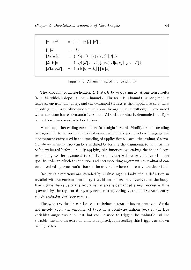
Chapter 6. Denotational semantics of Core Fudgets 64
[[� ! � 0]] = " ["" [[� ]]; " [[� 0]]]
[[x ]]o = x ![o]
[[�x :E ]]o = (�f )(o![f ] j �f ?[x ; b]:[[E ]]b)
[[E F ]]o = (�c)([[E ]]c j c?[f ]:(�x )(f ![x ; o] j [[x := F ]]))
[[Fix x :E ]]o = (�x )([[x := E ]] j [[E ]]o)
Figure 6.5: An encoding of the �-calculus
The encoding of an application E F starts by evaluating E . A function results
from this which is deposited on a channel c. The term F is bound to an argument x
using an environment entry, and the evaluated term E is then applied to this. This
encoding models call-by-name semantics as the argument x will only be evaluated
when the function E demands its value. Also if its value is demanded multiple
times then it is re-evaluated each time.
Modelling other calling-conventions is straightforward. Modifying the encoding
in Figure 6.5 to correspond to call-by-need semantics just involves changing the
environment entry used in the encoding of application to cache the evaluated term.
Call-by-value semantics can be simulated by forcing the arguments to applications
to be evaluated before actually applying the function by sending the channel cor-
responding to the argument to the function along with a result channel. The
speci�c order in which the function and corresponding argument are evaluated can
be controlled by synchronisation on the channels where the results are deposited.
Recursive de�nitions are encoded by evaluating the body of the de�nition in
parallel with an environment entry that binds the recursive variable to the body.
Every time the value of the recursive variable is demanded a new process will be
spawned by the replicated input process corresponding to the environment entry
which evaluates the recursive call.
The type translation can be used to induce a translation on contexts. We do
not merely apply the encoding of types in a pointwise fashion because the free
variables range over channels that can be used to trigger the evaluation of the
variable. Instead an extra channel is required, representing this trigger, as shown
in Figure 6.6.

Chapter 6. Denotational semantics of Core Fudgets 65
[[x1 : �1; :::; xn : �n ]] = x1 :"" [[�1]]; :::; xn :"" [[�n ]]
Figure 6.6: An encoding of type contexts
6.4.1 An Example
As an example of the �-calculus encoding, we illustrate the behaviour of the iden-
tity term. In this example, we make use of the transition relation de�ning the
�-calculus semantics, and also a relation, �, de�ned by the following equations:
(�x )P � P if x 62 fv(P)
(�x )(�x?[y ] j P) � P if x 62 fv(P):
This relation allows us to eliminate unused private variables and replicated input
processes that can never receive any input. The following sequence of equivalences
and transitions illustrates the behaviour of the identity term:
[[(�x :x )E ]]o
= (�c)([[�x :x ]]c j c?[f ]:(�x )(f ![x ; o] j [[x := E ]]))
= (�c)((�f )(c![f ] j �f ?[x ; b]:[[x ]]b) j c?[f ]:(�x )(f ![x ; o] j [[x := E ]]))��! (�c; f )(�f ?[x ; b]:[[x ]]b j (�x )(f ![x ; o] j [[x := E ]])):
The identity function is already a value here, and so no evaluation is required
and the channel f is immediately communicated along c. The next transition
corresponds to the actual application of the function to the argument:
��! (�c; f )(�f ?[x ; b]:[[x ]]b j (�x )([[x ]]o j [[x := E ]])):
The replicated input process can be eliminated now as there is no way in which it
can receive input:
� (�x )([[x ]]o j [[x := E ]])
= (�x )(x ![o] j �x?[c]:[[E ]]c):
Finally, we evaluate the body of the function, which forces us to lookup the de�-
nition of the variable x in the environment entry, yielding the term E :
��! (�x )(�x?[c]:[[E ]]c j [[E ]]o)
� [[E ]]o:

Chapter 6. Denotational semantics of Core Fudgets 66
The resulting �-calculus term [[E ]]o corresponds exactly to the encoding of the
original term if we had �-reduced the application of the identity function. In the
next chapter we will show how we can formally capture the equivalence of these
terms using the concept of bisimulation.
6.5 A �-calculus semantics of stream processors
The encoding of the �-calculus leads to a natural extension for representing stream
processors. A stream processor is represented similarly to a function, as a channel
on which two channels are expected to be received. These two channels correspond
to the input and output stream to use for the stream processor. In general the
translation of an arbitrary stream processor, S , will be of the form:
[[S ]]o = (�s)(o![s] j s?[in; out ]:P):
The process P may transmit the in and out channels along another channel that
represents a stream processor. This corresponds to passing the input and output
streams onto a continuation stream processor and is used in the translation of terms
involving GetSP and PutSP because both of these take continuation arguments.
Note that the input from the channel s is not replicated as the input and output
streams will only be sent once. To simplify the presentation of the encoding, we
de�ne some notation:
De�nition 6.2 (Stream processor encoding) We de�ne dPe to be a �-calculus
process corresponding to a generic stream processor whose input and output streams
are located by the channels in and out. The behaviour of this stream processor is
speci�ed by the �-calculus process P:
dPe = (�s)(o![s] j s?[in; out ]:P):
De�nition 6.3 (Stream processor instantiation) We de�ne ahin; outi to cor-
respond to the instantiation of the stream processor located by the channel a with
the input and output streams in and out:
ahin; outi = a?[s]:s![in; out ]:

Chapter 6. Denotational semantics of Core Fudgets 67
Streams themselves will be modelled by unbounded bu�ers, thus considering
the wires between stream processors as bu�ers. This ensures that no constraints
are made on the possible order in which the actions of individual stream processors
are undertaken.
6.5.1 Lists
Before considering the actual encoding of atomic and composite stream processors
we describe how lists can be encoded in the �-calculus. These will be used in
the next section to model unbounded bu�ers which are essential in the encoding
of stream processors. This is because we will consider the wires between stream
processors as unbounded bu�ers. Two parameterised processes are introduced
corresponding to the basic operations for constructing lists, along with a type
synonym, and are presented in Figure 6.7.
List � = Fix L: " [" []; " [�;L]]
Nil(r) = (�l)(r ![l ] j �l?[n; c]:n![])
Cons(h; t ; r) = (�l)(r ![l ] j �l?[n; c]:c![h; t ])
Figure 6.7: An encoding of lists
The process Nil(r) creates a new channel corresponding to an empty list and
deposits it on the channel r . The list can be interrogated by sending two channels
along it to test if the list is empty, or composed of an element followed by a list.
Similarly, the process Cons(h; t ; r) creates a new channel corresponding to a list
which has h as its head element, and is followed by the list t . The type synonym
List � denotes the type of lists with elements of type � . This synonym makes use
of recursive types as the tail of a nonempty list is another list of the same type.
It will be useful to have a reversing operation on lists and this is de�ned as
the Rev process shown in Figure 6.8. Rev(l ; r) reverses the list l and deposits the
reversed list on the channel r . This makes use of an auxiliary process, Rev 0(l ; a; r)
that uses an accumulating parameter. Rev 0(l ; a; r) reverses the list l and attaches
it to the front of the list a, with the �nal list being deposited on the result channel
r . The list a acts as an accumulating parameter. The list l is interrogated and if
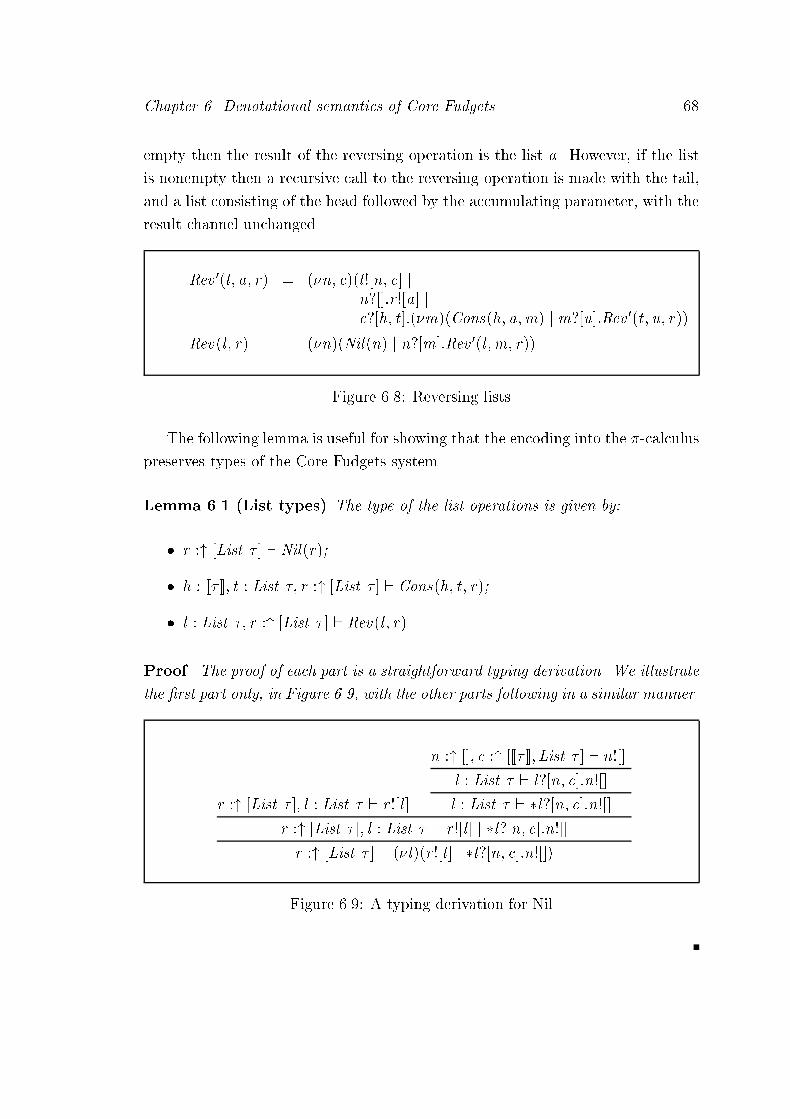
Chapter 6. Denotational semantics of Core Fudgets 68
empty then the result of the reversing operation is the list a. However, if the list
is nonempty then a recursive call to the reversing operation is made with the tail,
and a list consisting of the head followed by the accumulating parameter, with the
result channel unchanged.
Rev 0(l ; a; r) = (�n; c)(l ![n; c] jn?[]:r ![a] jc?[h; t ]:(�m)(Cons(h; a;m) j m?[u]:Rev 0(t ; u; r))
Rev(l ; r) = (�n)(Nil(n) j n?[m]:Rev 0(l ;m; r))
Figure 6.8: Reversing lists
The following lemma is useful for showing that the encoding into the �-calculus
preserves types of the Core Fudgets system.
Lemma 6.1 (List types) The type of the list operations is given by:
� r :" [List � ] ` Nil(r);
� h : [[� ]]; t : List �; r :" [List � ] ` Cons(h; t ; r);
� l : List �; r :" [List � ] ` Rev(l ; r).
Proof. The proof of each part is a straightforward typing derivation. We illustrate
the �rst part only, in Figure 6.9, with the other parts following in a similar manner.
r :" [List � ]; l : List � ` r ![l ]
n :" []; c :" [[[� ]];List � ] ` n![]
l : List � ` l?[n; c]:n![]
l : List � ` �l?[n; c]:n![]
r :" [List � ]; l : List � ` r ![l ] j �l?[n; c]:n![]
r :" [List � ] ` (�l)(r ![l ] j �l?[n; c]:n![])
Figure 6.9: A typing derivation for Nil

Chapter 6. Denotational semantics of Core Fudgets 69
6.5.2 Unbounded bu�ers
We can now describe how to encode unbounded bu�ers by using lists. Three new
processes are introduced corresponding to the construction and destruction oper-
ators for the bu�ers. They are de�ned in Figure 6.10 along with a type synonym
for bu�ers.
Bu�er � = " [List � ]
Empty(r) = (�b)(r ![b] j Nil(b))
Insert(x ; b; a) = b?[l ]:(Cons(x ; l ; b) j a![])
Remove(b; r) = b?[l ]:(�s)(Rev(l ; s) j(�n; c)(s?[rl ]:rl ![n; c] j
(n?[]:b![l ] j Remove(b; r)) jc?[h; t ]:r ![h]:Rev(t ; b)))
Figure 6.10: Bu�ers
The process Empty(r) creates a new unbounded bu�er which is initially empty.
The bu�er is modelled as a list which is created using the Nil(b) process. Elements
are inserted into the bu�er by the process Insert(x ; b; a), which adds the element
represented by x to the bu�er b. This �rst obtains exclusive access to the list by
retrieving the channel corresponding to the list modelling the bu�er. Once this
is done then a new list is constructed using the Cons(x ; l ; b) process, with the
resulting list deposited on the channel representing the bu�er, b. The channel
a acts as an acknowledgement to the process requesting the insertion, indicating
when the operation has actually taken place. Removal of elements is handled by
the Remove(b; r) process, which �rst retrieves the list corresponding to the bu�er
ensuring exclusive access. Next, this list is reversed in preparation for removing
the last element, giving a �rst-in �rst-out semantics to the bu�er. The reversed list
is interrogated and if empty then the original list representing the bu�er is output
on b allowing other processes to use the list. In parallel with this, the original
request to remove an element is repeated since the attempt to remove an element
failed due to the bu�er being empty. If the reversed list is non-empty then the
head element of the list is sent to the result channel r , while the tail is reversed
again to obtain the new list modelling the resulting bu�er which is deposited on

Chapter 6. Denotational semantics of Core Fudgets 70
the channel b allowing other processes to use the modi�ed bu�er. The types of the
bu�er operations are given by the following lemma:
Lemma 6.2 (Bu�er types) The type of the bu�er operations are given by:
� r :" [Bu�er � ] ` Empty(r);
� x : �; a :" []; b : Bu�er � ` Insert(x ; b; a);
� b : Bu�er �; r :" [� ] ` Remove(b; r).
Proof. Follows similarly to lemma 6.1.
We can now consider the type translation of stream processors, based on the
earlier generic de�nition of how stream processors are translated to the �-calculus.
A stream processor is translated to a process expecting to receive two channels
representing its input and output streams. Bu�ers are used to represent these
streams, and so the type translation is as shown in Figure 6.11. We note that the
type of the values stored in the bu�ers is not simply the type of values on the
streams, because the values are represented using environment entries.
[[SP � � 0]] = " [Bu�er "" [[� ]];Bu�er "" [[� 0]]]
Figure 6.11: An encoding of stream processor types
6.5.3 Atomic stream processors
The encoding of atomic stream processors is shown in Figure 6.12. The NullSP
construct is encoded using the dPe notation, where P is just the inactive pro-
cess. The translation of the term GetSP E is similar to the application of a
�-abstraction. However, the argument to apply to the function E is retrieved from
the input stream using the Remove process. The result of this application is in-
stantiated with the input and output streams. The third form of atomic stream
processor PutSP E F , is encoded by using an environment entry representing the
output term. A channel corresponding to this term is sent on the output stream
using the Insert process. After this has taken place then the continuation stream
processor F is evaluated and instantiated with the input and output streams.

Chapter 6. Denotational semantics of Core Fudgets 71
[[NullSP]]o = d0e
[[GetSP E ]]o = d(�r)(Remove(in; r) jr?[x ]:(�b)([[E ]]b j
b?[f ]:(�k)(f ![x ; k ] j khin; outi))e
[[PutSP E F ]]o = d(�x )([[x := E ]] j(�a)(Insert(x ; out ; a) j
a?[]:(�d)([[F ]]d j dhin; outi))e
Figure 6.12: An encoding of atomic stream processors
6.5.4 Composite stream processors
Next, we consider the composite stream processors starting with serial composition,
which is encoded by creating an intermediate stream between the two stream
processors being composed. The expressions corresponding to the two stream
processors are evaluated and the �-calculus channels locating their results are used
to instantiate the input and output streams. The rightmost stream processor is
instantiated with the overall input stream of the composition for its input stream.
Its output stream is instantiated with the new intermediate stream, which is also
used as the input stream of the leftmost stream processor. Finally, the output
stream of the leftmost stream processor is instantiated with the overall output
stream of the composition. The entire encoding is shown in Figure 6.13.
[[E >==< F ]]o = d(�l ; r ; s)([[E ]]l j[[F ]]r jEmpty(s) js?[mid ]:(lhmid ; outi j rhin;midi)e
Figure 6.13: An encoding of serial composition
Parallel composition requires the input stream to be split into two duplicate
streams. Assuming we can construct a process to accomplish this splitting of
streams then the encoding of parallel composition is as shown in Figure 6.14.
The two stream processors being composed are evaluated to obtain channels cor-
responding to them. Next, two new bu�ers are constructed and used in the to

Chapter 6. Denotational semantics of Core Fudgets 72
instantiate the input streams of the two stream processors. These two bu�ers re-
sult from the Split(in; l ; r) process which splits the input stream represented by
the channel in into two duplicate streams represented by the channels l and r ,
such that any values sent on the in stream are forwarded to both of the duplicate
streams.
[[E >�< F ]]o = d(�s; t)([[E ]]s j [[F ]]t j (�lb; rb)(Empty(lb) j Empty(rb) jlb?[l ]:rb?[r ]:(Split(in; l ; r) j
shl ; outi j thr ; outi)))e
Figure 6.14: An encoding of parallel composition
Using the de�nition of unbounded bu�ers from the previous section we can
de�ne the Split process. This process reads some input from the speci�ed input
stream, in, and continues by inserting the value read into the two bu�ers speci�ed
by l and r . Once both insertions have been acknowledged then the Split process
recursively calls itself. It must wait for both acknowledgements to ensure that the
order of values in the two bu�ers corresponds to that of the input stream in. The
overall de�nition of the Split process is shown in Figure 6.15.
Split(in; l ; r) = (�t)(Remove(in; t) j t?[x ]:(�a)(Insert(x ; l ; a) jInsert(x ; r ; a) ja?[]:a?[]:Split(in; l ; r)))
Figure 6.15: Splitting of streams
Next, we consider the looping construct LoopSP, which also requires the use
of unbounded bu�ers. The stream processor in the feedback loop is evaluated and
instantiated with the overall input stream and an output stream corresponding to
a new bu�er. This new bu�er is split into two separate bu�ers corresponding to
the overall output stream and the overall input stream by using the Split process.
The entire encoding of feedback is shown in Figure 6.16.

Chapter 6. Denotational semantics of Core Fudgets 73
[[LoopSP E ]]o = d(�ob)([[E ]]s j Empty(ob) job?[b]:(shin; bi j Split(b; out ; in))e
Figure 6.16: An encoding of feedback
Finally, we must consider the encoding of the dynamic construct, DynSP. The
idea used in the encoding is to introduce two extra processes, an input manager
and an output manager that handle the input and output streams, and also the
communication with the active stream processor:
InputManager
ActiveStreamProcessor
OutputManager
InputStream
OutputStream
The input manager analyses values of the sum type on the overall input stream
and if they are right injections then they are considered as input for the currently
active stream processor. Otherwise the value is a new stream processor, which will
be used to replace the currently active stream processor.
The output manager's job is to receive output from the currently active stream
processor and forward it to the overall output stream. It also may receive messages
from the input manager indicating that the currently active stream processor has
changed. Whenever this occurs then the output manager must ignore output from
the previously active stream processor and start forwarding the output from the
newly active stream processor to the overall output stream.
The encoding of the dynamic construct creates two new bu�ers which are used
to instantiate the initial stream processors input and output streams. In parallel

Chapter 6. Denotational semantics of Core Fudgets 74
with this the input and output manager are started and supplied with the over-
all input and output streams and the two bu�ers corresponding to the streams
connected to the initial stream processor.
[[DynSP E ]]o = d(�s)([[E ]]s j (�t ; u; n)(Empty(t) j Empty(u) jt?[ain]:u?[aout ]:(shain; aouti jIM (in; ain; n) j OM (out ; aout ; n)))e
IM (in; ain; n) = Remove(in; s) js?[x ]:(�l ; r)(x ![l ; r ] j
l?[v ]:(�t ; u)(Empty(t) j Empty(u) jt?[ain]:u?[aout ]:(v ![sp] j
sphain; aouti jn![aout ]:IM (in; ain; n))) j
r?[y ]:Insert(ain; y ; a) j a?[]:IM (in; ain; n))
OM (out ; aout ; n) = Remove(aout ; r) j(r?[x ]:(Insert(out ; x ; a) j a?[]:OM (out ; aout ; n)) +n?[aout ]:OM (out ; aout ; n))
Figure 6.17: An encoding of dynamic stream processors
The output manager has to process input from two locations, the output bu�er
from the active stream processor and noti�cations from the input manager indicat-
ing a change in the active stream processor. The encoding uses the choice construct
of the �-calculus to decide at any one time which of these two possible sources of
input to read from. This is the only place in the semantics where the choice con-
struct is used, and it is an instance of guarded choice since both branches begin
by performing input from a channel variable. This yields a semantics where the
currently active stream processor can continue to produce output for a inde�nite
amount of time before being replaced by a new stream processor. However, the
encoding does guarantee that, after an input message requesting a change of the
active stream processor, all following input will be processed by the new stream
processor.
The following proposition shows that the type structure of the Core Fudgets
language is preserved by the encoding into the �-calculus. The type of the channel
a is equivalent to " [[� ]] up to type equality, as this corresponds to the location of
the result of evaluating the term E which we know has type � .

Chapter 6. Denotational semantics of Core Fudgets 75
Proposition 6.1 (Type soundness) If � ` E : � then [[�]]; a : � 0 ` [[E ]]a and
� 0 '" [[� ]].
Proof. The proof proceeds by induction on the structure of the derivation of
� ` E : � . We show three cases. The other cases are similar, with some using
Lemmas 6.1 and 6.2 to derive appropriate types for the list and bu�er operations
used in the encoding of term E.
Case � ` n : num where n 2 f0; 1; :::g. From the (Output) rule we have the deriva-
tion [[�]]; a :" [[num]] ` a![n] because [[num]] = num, and thus we obtain the
derivation [[�]]; a :" [[num]] ` [[n]]a as required.
Case � ` �x :E : � ! � 0 where �; x : � ` E : � 0. By induction we have the deriva-
tion [[�; x : � ]]; b :" [[� 0]] ` [[E ]]b, and by using weakening we can show that
[[�]]; f :" ["" [[� ]]; " [[� 0]]]; x :"" [[� ]]; b :" [[� 0]] ` [[E ]]b: From the (Input) and
(Repl) rules we can show that [[�]]; f :" ["" [[� ]]; " [[� 0]]] ` �f ?[x ; b]:[[E ]]b: Using
the (Output) rule we have that [[�]]; a :" [[� ! � 0]]; f :" ["" [[� ]]; " [[� 0]]] ` a![f ]
because [[� ! � 0]] = " ["" [[� ]]; " [[� 0]]]. Finally, using weakening, the (Prl) and
(Res) rules we can show that [[�]]; a :" [[� ! � 0]] ` (�f )(a![f ] j �f ?[x ; b]:[[E ]]b)
as required.
Case � ` NullSP : SP � � 0. Using weakening and the (Input) rule we can show
that [[�]]; a :" [[SP � � 0]]; s : [[SP � � 0]] ` s?[in; out ]:0: Now, since
[[SP � � 0]] =" [Bu�er �;Bu�er � 0] then by using the (Output) rule we have
that [[�]]; a :"" [Bu�er �;Bu�er � 0]; s :" [Bu�er �;Bu�er � 0] ` a![s]: Thus by
using the (Prl) and (Res) rules we obtain the derivation
[[�]]; a :"" [Bu�er �;Bu�er � 0] ` (�s)(a![s] j s?[in; out ]:0) which is equiv-
alent to [[�]]; a :" [[SP � � 0]] ` d0e as required.
This proof of type soundness is quite lengthy and would bene�t from machine
checking. This can be accomplished by building a type inference tool for the variant
of the pi -calculus being used.

Chapter 7
Reasoning about Core Fudgets
In the last chapter we described a formal semantics for Core Fudgets by using an
encoding into the �-calculus. This chapter reviews the theory of the �-calculus
and describes how we can use it to reason about Core Fudget programs.
Processes in the �-calculus can be compared using a behavioural equivalence.
The most often used method for de�ning such equivalences is the mathematical idea
of bisimulation. This equates two processes if their transition trees have the same
structure and the labels of the transitions are comparable. In Section 7.1 we review
this approach to de�ning equivalences for the �-calculus. The main contribution
of this chapter, in Section 7.1.2, is the de�nition of an equational theory for Core
Fudgets. This theory equates two Core Fudget terms if their corresponding �-
calculus encodings are bisimilar. This is illustrated by some examples in Section 7.2
where it is used to reason about Core Fudget programs. The chapter concludes
with a discussion of the advantages and disadvantages of using the �-calculus to
de�ne the semantics of the Core Fudgets language, and some alternative decisions
that could be taken in giving Core Fudgets a semantics.
7.1 Bisimulation for the �-calculus
The standard method of de�ning behavioural equivalences for process calculi is
to use bisimulations. A bisimulation on processes is an equivalence based on the
observable properties of the processes. However, there are many di�erent ways of
de�ning the observable properties which lead to numerous formulations of bisim-
ulation.
76

Chapter 7. Reasoning about Core Fudgets 77
The original de�nition of bisimulation is due to Park [Par81] and was developed
as a method for comparing automata. However, Milner later realized that this idea
of bisimulation could be used to formulate a precise behavioural equivalence for
the process calculus CCS [Mil85]. This is where we �nd the classical form of
bisimulation, which in the context of the �-calculus is often referred to as ground
bisimulation. This compares processes based purely upon the actions that they
can perform. However, because the �-calculus we presented in Chapter 5 has an
associated typing system then we must introduce the concept of a con�ned relation
before we de�ne ground bisimulation formally:
De�nition 7.1 (Con�ned relation) A set of relations, R� between processes
with the same context � is a con�ned relation if PR�Q implies � ` P and � ` Q.
We shall write � ` PRQ to mean that PR�Q, and usually omit any obvious type
information.
De�nition 7.2 (Ground simulation) A con�ned relation R between processes
is a ground simulation if � ` PRQ implies:
� if � ` P��! P 0 then 9Q 0:� ` Q
��! Q 0 and � ` P 0RQ 0.
Intuitively, we can think of this de�nition as requiring that we can complete all
diagrams of the following form (for simplicity we omit typing information):
P R Q P R Q
as
P 0
�
?P 0
�
?R Q 0
?
�
De�nition 7.3 (Ground bisimulation) A con�ned relation, S, is a ground bisim-
ulation if S and S�1 are ground simulations. Ground bisimilarity, �, is de�ned to
be the greatest such relation.
Here � corresponds to an action, and P��! P 0 means that the process P can evolve
by performing the transition labelled by the action � to the process P 0. The syntax
of actions is determined by the process calculi that we are using. For example, in
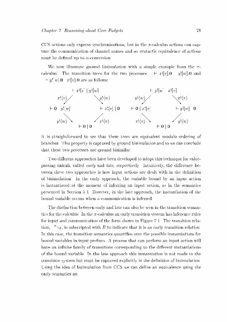
Chapter 7. Reasoning about Core Fudgets 78
CCS actions only express synchronisations, but in the �-calculus actions can cap-
ture the communication of channel names and so syntactic equivalence of actions
must be de�ned up to �-conversion.
We now illustrate ground bisimulation with a simple example from the �-
calculus. The transition trees for the two processes � ` x ![v ]:0 j y ![w ]:0 and
� ` y ![w ]:0 j x ![v ]:0 are as follows:
� ` x ![v ] j y ![w ]
���x !hvi @
@@y !hwiR
� ` 0 j y ![w ] � ` x ![v ] j 0
@@@y !hwi R �
��
x !hvi� ` 0 j 0
� ` y ![w ] j x ![v ]
���y !hwi @
@@x !hviR
� ` 0 j x ![v ] � ` y ![w ] j 0
@@@x !hvi R �
��
y !hwi� ` 0 j 0
It is straightforward to see that these trees are equivalent modulo ordering of
branches. This property is captured by ground bisimulation and so we can conclude
that these two processes are ground bisimilar.
Two di�erent approaches have been developed to adopt this technique for value-
passing calculi, called early and late, respectively. Intuitively, the di�erence be-
tween these two approaches is how input actions are dealt with in the de�nition
of bisimulation. In the early approach, the variable bound by an input action
is instantiated at the moment of inferring an input action, as in the semantics
presented in Section 5.4. However, in the late approach, the instantiation of the
bound variable occurs when a communication is inferred.
The distinction between early and late can also be seen in the transition seman-
tics for the calculus. In the �-calculus an early transition system has inference rules
for input and communication of the form shown in Figure 7.1. The transition rela-
tion,��!E , is subscripted with E to indicate that it is an early transition relation.
In this case, the transition semantics quanti�es over the possible instantiations for
bound variables in input pre�xes. A process that can perform an input action will
have an in�nite family of transitions corresponding to the di�erent instantiations
of the bound variable. In the late approach this instantiation is not made in the
transition system but must be captured explicitly in the de�nition of bisimulation.
Using the idea of bisimulation from CCS we can de�ne an equivalence using the
early semantics as:

Chapter 7. Reasoning about Core Fudgets 79
De�nition 7.4 (Early simulation) A con�ned relation R between processes is
an early simulation if � ` PRQ implies:
� if � ` P��!E P 0 then 9Q 0:� ` Q
��!E Q 0 and � ` P 0RQ 0.
Intuitively, we can think of this de�nition as requiring that we can complete all
diagrams of the following form (for simplicity we omit typing information):
P R Q P R Q
as
P 0
�
?EP 0
�
?ER Q 0
?E
�
De�nition 7.5 (Early bisimulation) A con�ned relation, S, is an early bisim-
ulation if S and S�1 are early simulations. Early bisimulation, �E , is de�ned to
be the greatest such relation.
(In)� ` ~v : ~� �(x ) '" [~� ]
� ` x?[~y ]:Px?h~z i�!E P [~z=~y ]
(Com)� ` P
(� ~y 0)x !h~yi�! E P 0 � ` Q
x?h~yi�!E Q 0
� ` P j Q��!E (�~y 0)(P 0 j Q 0)
~y 0 \ fn(Q) = ;
Figure 7.1: An early transition semantics
The corresponding late semantics is characterised by the inference rules shown
in Figure 7.2. The de�nition of late bisimulation is complicated by the fact that
input actions need to be treated as a special case:
De�nition 7.6 (Late simulation) A con�ned relation R between processes is a
late simulation if � ` PRQ implies:
� if � ` Pa?h~yi�!L P 0 then 9Q 0:� ` Q
a?h~yi�!L Q 0 and 8~z :� ` P 0[~z=~y ]RQ 0[~z=~y ];
� if � ` P��!L P 0 then 9Q 0:� ` Q
��!L Q 0 and � ` P 0RQ 0 for � 6= a?h~yi.

Chapter 7. Reasoning about Core Fudgets 80
De�nition 7.7 (Late bisimulation) A con�ned relation, S, is a late bisimula-
tion if S and S�1 are late simulations. Late bisimulation, �L, is de�ned to be the
greatest such relation.
(In) � ` x?[~y ]:Px?h~yi�!L P
(Com)� ` P
(� ~y 0)x !h~z i�! L P 0 � ` Q
x?h~yi�!L Q 0
� ` P j Q��!L (�~y 0)(P
0 j Q 0[~z=~y ])~y 0 \ fn(Q) = ;
Figure 7.2: A late transition semantics
In this dissertation, we will make use of early bisimulation. Our motivation
for this choice is twofold. Firstly, the transition system for the semantics of the
�-calculus in Section 5.4 facilitates a simpler de�nition of early bisimulation than
late bisimulation. In the late case, input actions must be dealt with separately in
the de�nition of bisimulation whereas in the early case a single clause is su�cient.
Secondly, the intuition behind early bisimulation is easier to understand, as the
instantiation of a bound variable occurs simultaneously with the choice of where
the input is occuring, whereas late bisimulation separates these two events.
To use bisimulation as the basis for an equational theory, where one expression
can be replaced by another that is semantically equivalent, it must be preserved
by as many of the operators of the language as possible. We can show that early
bisimulation is preserved by all of the following operators:
Proposition 7.1 If � ` P �E Q then we have the following:
1. if �(x ) ' ~� and �(~v) = ~� then � ` x ![~v ]:P �E x ![~v ]:Q;
2. � ` (�~x )P �E (�~x )Q;
3. if P and Q are guarded processes then if � ` G then � ` G j P �E G j Q
and � ` P j G �E Q j G;
4. if � ` R then � ` R + P �E R +Q and � ` P +G �E Q +G;
5. � ` �P �E �Q;

Chapter 7. Reasoning about Core Fudgets 81
6. if �(v) ' num and � ` R then � ` if v then P else R �E if v then Q else R
and � ` if v then R else P �E if v then R else Q;
7. if �(v) ' num and �(w) ' num and also
8. if �(v) ' num and �(w) ' num and also �(x ) '" [bool] then it follows
that � ` equal [v ;w ; x ]:P �E equal [v ;w ; x ]:Q.
9. if �(v) ' num and �(w) ' num and also �(x ) '" [num] then it follows
that � ` add [v ;w ; x ]:P �E add [v ;w ; x ]:Q.
Proof. The proof is standard and follows the corresponding proof for the original
�-calculus [MPW89]. We only consider output pre�x. De�ne:
S� = f(x ![~v ]:P ; x ![~v ]:Q) j � ` P �E Qg[ �E :
We proceed by a case analysis on the rule used to infer a transition for � ` x ![~v ]:P.
There is only one possibility due to the (Out) transition rule, and we have:
� ` x ![~v ]:Px !h~vi�! P :
From the (Out) rule we also have that � ` x ![~v ]:Qx !h~vi�! Q, and because � `
P �E Q then PS�Q as required. The other parts follow in a similar manner,
with the technique of bisimulation up to restriction, as used by Milner, Parrow and
Walker [MPW89], useful in proving part (3).
Although early bisimulation is preserved by most of the operators of the language,
it is not preserved by input pre�xing. This is illustrated by the following two
�-calculus processes:
P = x?[] j y ![]
Q = x?[]:y ![] + y ![]:x?[]
which are obviously related by early bisimilarity. Unfortunately though, if we pre�x
the above two processes by an input yielding the processes a?[x ]:P and a?[x ]:Q
then these processes are not early bisimilar. This is because there is a transition
for the �rst process, a?[x ]:Pa?hyi�! y?[] j y ![]
��! 0, which cannot be matched by
the second, a?[x ]:Qa?hyi�! y?[]:y ![] + y ![]:y?[] 6
��!. Milner, Parrow and Walker solve
this problem by quantifying over all possible substitutions for free channel names,
resulting in early congruence:

Chapter 7. Reasoning about Core Fudgets 82
De�nition 7.8 (Early congruence) If � = ~x : ~� , then we de�ne a �-substitution
to be a substitution �[~v=~x ] where � ` ~v : ~� . Early congruence, �cE , is the least con-
�ned relation such that:
� � ` P �cE Q i� � ` P [~v=~x ] �E Q [~v=~x ] for all �-substitutions �[~v=~x ].
Relations will be denoted to be congruences by the addition of a superscript `c'.
Proposition 7.2 If � ` P �cE Q then � ` x?[~y ]:P �c
E x?[~y ]:Q.
Proof. We show that the following relation is an early congruence:
S� = f(x?[~y ]:P ; x?[~y ]:Q) j � ` P �cE Qg:
Proceeding by case analysis on the transition rule used to infer a transition for
� ` x?[~y ]:P, we have only one possibility, due to the (In) rule:
� ` vi : �i for i 2 f1::ng �(x ) '" [~� ]
� ` x?[~y ]:Px?h~vi�! P [~v=~y ] .
Similarly, we can derive the transition � ` x?[~y ]:Qx?h~vi�! Q [~v=~y ]. However, because
� ` P �cE Q then it must be that � ` P [~v=~y]SQ [~v=~y ] as required.
It follows from the de�nition of �cE that any two terms related by �E are also re-
lated by �cE and thus proposition 7.1 holds for �c
E . Using this with proposition 7.2
we can conclude that early congruence is preserved by all of the operators of the
�-calculus. This is important as it allows us to consider using early congruence
as the basis of an equational theory, where we can replace a subterm of a process
with another early congruent subterm.
An alternative approach to obtaining a relation that is preserved by all opera-
tors of the language is the concept of open bisimulation studied by Sangiorgi [San93].
This integrates the instantiation of names into the de�nition of bisimulation in such
a manner that it is preserved by all operators of the language. We do not consider
open bisimulation further in this dissertation, although it could be used to prove
all of the results we consider in Section 7.2. Whether it simpli�es these proofs is
an open question, as the size of relations required to de�ne open bisimulations can
be large, although its complexity may be lower than that of early congruence.

Chapter 7. Reasoning about Core Fudgets 83
7.1.1 Weak bisimulations
The bisimulations reviewed so far have all been strong bisimulations. They all
consider the internal moves of processes { the communication actions { in the
same manner as the other actions corresponding to the external behaviour of the
processes. This results in rather strict relations, and it is often the case that we
wish to abstract away from the internal details of processes.
Bisimulations that abstract away from communication actions which represent
the internal behaviour of processes are called weak bisimulations. They correspond
to a weak behavioural equivalence that equates processes only based upon their
external behaviour and not the internal behaviour of the processes. The standard
formulation of these bisimulations involves de�ning a concept of weak transitions:
De�nition 7.9 (Weak transitions) Let =) be the re exive and transitive clo-
sure of��!, and
�=) be the relational composition =) �
��! � =). A weak
transition,b�
=) is de�ned as:
b�=)=
8<:
�=) if � 6= �
=) otherwise
A weak bisimulation is de�ned by requiring that strong transitions are matched
by weak ones. For example, the de�nition of weak early bisimilarity is given by:
De�nition 7.10 (Weak early simulation) A con�ned relation R between pro-
cesses is a weak early simulation if � ` PRQ implies:
� whenever � ` P��!E P 0 then 9Q 0:� ` Q
�=)E Q 0 and � ` P 0RQ 0.
De�nition 7.11 (Weak early bisimilarity) A con�ned relation, S, is a weak
early bisimulation if S and S�1 are weak early simulations. Weak early bisimulation
�E is de�ned to be the greatest such relation.
In a similar manner to strong early bisimilarity, we must explicitly de�ne a
congruence to handle the fact that weak early bisimilarity is not preserved by
input pre�xes. We denote the largest weak early congruence as �cE , which is
de�ned analogously to the early congruence of De�nition 7.8.

Chapter 7. Reasoning about Core Fudgets 84
Proposition 7.3 Weak early congruence �cE is preserved by all of the operators
of the �-calculus.
Proof. Follows in a similar manner to propositions 7.1 and 7.2.
If we allowed unrestricted choice in our variant of the �-calculus then this proof
fails. However, the encoding of Core Fudgets in Chapter 6 only makes use of
guarded choice and so we only included guarded choice in our �-calculus variant
to ensure that this proof does not fail.
7.1.2 Equivalence for Core Fudgets
The theory presented in this chapter so far is standard for the �-calculus. In this
section we make the main contribution of this chapter by de�ning an equational
theory for Core Fudgets. We propose using weak early congruence as an equivalence
for the Core Fudgets language. A weak equivalence is preferable over a strong one
as we do not wish to distinguish between Core Fudget terms that only di�er in
their internal behaviour. For example, intuitively we would expect the following
terms to be equivalent:
PutSP x NullSP
GetSP (�y :PutSP x NullSP)>==< PutSP z NullSP:
However, a strong bisimulation does not relate these terms and hence is not an
appropriate choice for the basis of an equivalence on Core Fudget terms. A weak
bisimulation will relate these terms, capturing the fact that we do not wish the
observer to discriminate terms based on their internal behaviour. We can now
de�ne an equivalence on Core Fudget terms by introducing an equational theory:
De�nition 7.12 (Equational theory) An equational theory of Core Fudgets,
Tcf , consists of equations of the form � ` E = F : � , asserting that the two
terms E and F are equivalent. Formally, we de�ne this equivalence relation as:
� � ` E = F : � if and only if [[�]]; a :" [[� ]] ` [[E ]]a �cE [[F ]]a:
It is straightforward to check that weak early bisimulation, and hence weak early
congruence, is actually an equivalence.

Chapter 7. Reasoning about Core Fudgets 85
Proposition 7.4 Weak early bisimulation, �E , is an equivalence relation.
Proof. By de�nition �E is symmetric, and it is straightforward to show f(E ;E ) j
� ` E �E Eg to be a weak early bisimulation thus proving re exivity. Similarly,
we prove transitivity by showing �E � �E to be a weak early bisimulation.
7.2 Examples
In this section we illustrate the equational theory from De�nition 7.12 by formally
analysing some Core Fudget programs. We start by revisiting the identity stream
processor example from Section 4.2.1, and examine its semantics according to the
�-calculus encoding of Core Fudgets.
7.2.1 The identity stream processor
We recall the de�nition of the identity stream processor in Core Fudgets:
idSP = Fix i :(GetSP (�x :PutSP x i)):
According to the �-calculus de�nition, the semantics of this program is given by
the following process:
[[idSP ]]o
= (�i)([[i := GetSP (�x :PutSP x i)]] j
[[GetSP (�x :PutSP x i)]]o)
= (�i)(�i?[c]:[[GetSP (�x :PutSP x i)]]c j
[[GetSP (�x :PutSP x i)]]o):
We now concentrate on the body of the de�nition because it occurs in both of the
branches of the parallel composition. The encoding of this term yields the process:
[[GetSP (�x :PutSP x i)]]o
= d(�r)(Remove(in; r) j
r?[x ]:(�b)([[�x :PutSP x i ]]b j
b?[f ]:(�k)(f ![x ; k ] j khin; outi)))e
= d(�r)(Remove(in; r) j
r?[x ]:(�b)((�f )(b![f ] j �f ?[x ; b][[PutSP x i ]]b) j
b?[f ]:(�k)(f ![x ; k ] j khin; outi)))e:

Chapter 7. Reasoning about Core Fudgets 86
The semantics of the �-calculus does not allow us to reduce the communication
on the channel b because it is guarded by an input pre�x. However, using the
weak early congruence described in the previous section we can reduce the com-
munication but weakening the statement to indicate the equivalence as weak early
congruence:
�cE d(�r)(Remove(in; r) j
r?[x ]:(�f )(�f ?[x ; b][[PutSP x i ]]b j
(�k)(f ![x ; k ] j khin; outi)))e:
Similarly, we can now consider the reduction of the communication possible on
the channel f . The replicated input process on f will never be able to receive any
input after this communication and can also be eliminated, yielding the equivalent
process:
�cE d(�r)(Remove(in; r) j
r?[x ]:(�k)([[PutSP x i ]]k j khin; outi))e:
Now, we can expand out the remaining Core Fudget term and the stream processor
instantiation khin; outi, to obtain the process:
= d(�r)(Remove(in; r) j
r?[x ]:(�k)((�s)(k ![s] j
s?[in; out ]:(�y)([[y := x ]] j
(�a)(Insert(y ; out ; a) j
a?[]:(�d)([[i ]]d j dhin; outi)))) j
k?[s]:s![in; out ]))e:
Note that we have not used the simpler notation d e in the expansion of the bfPutSP
term as this would have hidden the communication that is possible on the channel
k . Again, we consider the reduction corresponding to this communication that
yields an equivalent process up to weak early congruence:
�cE d(�r)(Remove(in; r) j
r?[x ]:(�s)(s?[in; out ]:(�y)([[y := x ]] j
(�a)(Insert(y ; out ; a) j
a?[]:(�d)([[i ]]d j dhin; outi))) j
s![in; out ]))e:

Chapter 7. Reasoning about Core Fudgets 87
Once more, we have a possible reduction corresponding to the communication on
the channel s, and this results in the equivalent process:
�cE d(�r)(Remove(in; r) j
r?[x ]:(�y)([[y := x ]] j
(�a)(Insert(y ; out ; a) j
a?[]:(�d)([[i ]]d j dhin; outi))))e:
We can eliminate the use of the environment entry as the channel x corresponds
to a term removed from the input stream. All the channels communicated along
input streams correspond to triggers for evaluating the actual terms being sent,
and so the environment entry in the above process just introduces an extra level
of indirection:
�cE d(�r)(Remove(in; r) j
r?[x ]:(�a)(Insert(x ; out ; a) j
a?[]:(�d)([[i ]]d j dhin; outi))))e:
This simpli�ed process can be replaced into the original expansion of idSP where
it occurs twice due to the recursive nature of the stream processor. However, the
above form of the process clearly illustrates the behaviour of the identity stream
processor. Initially it removes an element from the input stream, and then inserts
this into the output stream. Once the insertion has been performed it evaluates the
term i , corresponding to a recursive call to the stream processor. This call yields
a stream processor which is then instantiated with the same input and output
streams. The two channels r and a are used to ensure the sequentiality of the
reading and writing from the input and to the output stream, respectively.
7.2.2 Commutativity of parallel composition
The next example we inspect corresponds to parallel composition of stream pro-
cessors being commutative. This is an equational rule that one would expect to
hold given the informal description of the semantics stated in Chapter 3. Here, we
formally prove this equational rule which can be stated as:
� ` E >�< F = F >�< E : SP � � 0:

Chapter 7. Reasoning about Core Fudgets 88
Using the de�nition of our equational theory this rule is valid if and only if the
corresponding encoding into the �-calculus is a correct statement:
�; a :" [[SP � � 0]] ` [[E >�< F ]]a �cE [[F >�< E ]]a:
Starting with the left hand side of this equation we show how we can derive the
right hand side:
[[E >�< F ]]o
= d(�s; t)([[E ]]s j [[F ]]t j (�lb; rb)(Empty(lb) j Empty(rb) j
lb?[l ]:rb?[r ]:(Split(in; l ; r) j shl ; outi j thr ; outi)))e:
By renaming the local channel names, we can show this to be �-equivalent to the
following process:
�� d(�s; t)([[E ]]t j [[F ]]s j (�lb; rb)(Empty(lb) j Empty(rb) j
lb?[l ]:rb?[r ]:(Split(in; l ; r) j thl ; outi j shr ; outi)))e:
Now, using weak early congruence we can reorder the parallel processes to give:
�cE d(�s; t)([[F ]]s j [[E ]]t j (�lb; rb)(Empty(lb) j Empty(rb) j
lb?[l ]:rb?[r ]:(Split(in; l ; r) j thl ; outi j shr ; outi)))e:
which is almost the right hand side we desire, except that the channels l and r are
swapped in the processes shr ; outi and thl ; outi. The proof of commutativity can
be completed if we can show that:
Split(in; l ; r) j thl ; outi j shr ; outi �cE Split(in; l ; r) j shl ; outi j thr ; outi:
We proceed by starting with the left hand side of this equation and renaming
channel variables, then we can rearrange the parallel processes using weak early
congruence:
Split(in; l ; r) j thl ; outi j shr ; outi
= Split(in; r ; l) j thr ; outi j shl ; outi
�cE Split(in; r ; l) j shl ; outi j thr ; outi
The remaining stage of the proof is to show that Split(in; r ; l) �cE Split(in; l ; r),
and this is straightforward since we can rearrange the Insert parallel processes in

Chapter 7. Reasoning about Core Fudgets 89
the de�nition of Split using weak early congruence. This completes the proof of
the original equation we set out to prove, verifying that parallel composition of
stream processors is indeed commutative according to the �-calculus semantics.
7.3 Analysis of �-calculus encoding
In this section we consider the advantages and disadvantages of using the �-calculus
for specifying the semantics of Core Fudgets. Reasons for using the �-calculus as
the basis of a semantics for Core Fudgets were discussed at the start of Chapter 5.
Here, we concentrate on the advantages of this approach that became apparent
during and after the development of the semantics. Particular emphasis is placed
on assessing the usefulness of the theory of the �-calculus for reasoning about Core
Fudget terms through the encoding into the �-calculus:
� There is no need to develop a new theory, as the theory of the �-calculus can
be drawn upon to induce a theory for Core Fudgets. There are numerous
de�nitions of equivalence for the �-calculus and an appropriate one for Core
Fudgets is weak early congruence as described in Section 7.1.1.
� The �-calculus encoding can be used as a reference implementation, by mak-
ing use of an implementation of the �-calculus. The PICT programming
language [PT97], based on the �-calculus, makes a particularly good base
for executing the �-calculus semantics. Although it does not provide direct
support for the synchronous calculus, the encoding given in Chapter 6 can
be modi�ed to use only asynchronous communication. PICT has a type
system very similar to that described in Chapter 6, and also supports poly-
morphism. This is useful as, in practice, most interesting stream processors
are polymorphic.
� As no new theory was required, the �-calculus provided a useful means for
exploring the possible semantic issues of the Core Fudgets language. This
language has some constructs whose precise semantic meaning is not entirely
clear, and various possibilities for their meaning exist. The �-calculus pro-
vided a formal mechanism for precisely specifying these di�erent alternatives
and gave insight into them.

Chapter 7. Reasoning about Core Fudgets 90
� It is possible to automate the checking of equivalences for the �-calculus
using tools such as the Mobility Workbench [VM94]. However, these tools
do not tend to work well with recursive �-calculus expressions. This is a
problem because the majority of interesting Core Fudget programs involve
recursion, whose encodings are recursive �-calculus processes.
Although the �-calculus has proved to be advantageous in developing a seman-
tics for Core Fudgets, there are also some serious disadvantages with this approach:
� The �-calculus is a very low level language in which the only means of com-
putation is communication. This leads to even relatively simple Core Fudget
terms having encodings that are large and complicated. The intuition behind
the semantics of the various constructs in the Core Fudgets language tend to
get lost in the exact details of these encodings.
� The most interesting Core Fudget terms tend to be recursive, and to prove
properties about such terms by using the theory of the �-calculus can be
complicated. The standard technique for proving bisimulations involving
such terms is coinduction [MT90, Pit94], but this can be di�cult to apply.
7.4 Semantic issues
During the development of the �-calculus semantics for Core Fudgets it became
clear that a number of semantic issues need to be addressed for any semantics of
Core Fudgets. Here we consider these issues and their possible solutions.
The original implementation of the Fudgets system evaluates stream processors
in a �xed order. This order is chosen to correspond to the demand of data, corre-
sponding to the demand driven nature of the Haskell language due to its laziness.
Two stream processors in series, A>==< B , are evaluated by �rst evaluating A.
If A can produce some output then this action is undertaken, and the residual of
A is recursively evaluated. Only when A requires input to continue is the stream
processor B evaluated, and then only far enough to satisfy the demand for data
from A. Specifying such a �xed order of evaluation in the semantics avoids the
need to consider the wires between stream processors as unbounded bu�ers.
An alternative semantic choice is to consider no particular evaluation order,
which is the decision taken by the semantics in the previous chapter. This has

Chapter 7. Reasoning about Core Fudgets 91
the e�ect of requiring the wires between stream processors to be considered as
unbounded bu�ers.
Another place in the semantics where various choices exist is the semantics
of the merging operations required in parallel composition and feedback. It is
hard to justify any other interpretation of the merge for parallel composition than
a nondeterministic merge. However, in the case of feedback there are practical
arguments for the merging operation being deterministic. Consider a graphical
program consisting of a group of buttons, one of which is always depressed whilst
the others are not. When the user presses one of the buttons it becomes the
depressed one, and the currently depressed button is raised. One way of modelling
this using stream processors is to represent each of the buttons with a single stream
processor. All of these stream processors are combined in parallel, and this overall
stream processor is then combined using feedback. The feedback is required so
that when one of the buttons is pressed it can indicate to all the others that it
has just been depressed. The button that was depressed receives the information
about the new depression and so can raise itself. However, if we let the overall
input to the feedback be used to programmatically depress a button, then we run
into problems. This model of the program will only work in a reasonable manner if
the merge operation on the input side of feedback biases towards the feedback loop.
If not, then it would be possible to receive a programmatic message indicating a
depression of a button before the message indicating an actual action by the user
depressing a button.

Chapter 8
Operational semantics of Core
Fudgets
In the previous chapter we presented a formal semantics for the Core Fudget lan-
guage using an encoding into the �-calculus. Although this captured the precise
meaning of Core Fudget programs the encoding of even trivial Core Fudget pro-
grams can be large and unwieldy �-calculus processes. More importantly the
intuition behind the semantics is hidden by the detail in these processes. This
chapter describes a direct operational semantics for Core Fudgets solving these
problems. This semantics is inspired by the lessons learnt from the denotational
semantics of Chapter 6, and is based on a labelled transition system. We examine
some bisimulation equivalences and �nally choose a variant of weak higher-order
bisimulation, which we show to be a congruence. The semantics is closely related
to the semantics that Ferriera et. al [FHJ95] developed for Concurrent ML. There
are some di�erences between the operational and denotational semantics but we
believe these can be easily eliminated yielding the relationship shown in Figure 8.1.
�-calculus
Core
Fudgets
Denotational
Semantics (Chapter 6)
Operational
Semantics (Chapter 8)
�-calculus (Chapter 5)
Transition
Semantics of
Trees
Figure 8.1: The relationship between the semantics
92

Chapter 8. Operational semantics of Core Fudgets 93
8.1 An Operational semantics
In this section we de�ne a structured operational semantics for Core Fudgets using
ideas from Milner's concurrent language CCS [Mil85]. This semantics was inspired
by some of the lessons learnt from the denotational semantics described in Chap-
ter 6. We believe that an operational semantics is more intuitive and simpler than
the denotational semantics. Insight into di�erent implementations of the Fudgets
system is easier with this semantics, and coinductive proofs [MT90, Pit94] are also
simpler.
The semantics is de�ned in terms of a labelled transition system that charac-
terises the immediate observations of Core Fudget programs. A labelled transition
system is a triple, (S ;A;��!), comprising a set S of states, a set A of actions used
to label transitions, and a transition relation,��!� S � S for each � 2 A. We
extend this de�nition to include a typing context, in the same way as was done for
the operational semantics of the �-calculus in Section 5.4. The transition relation
is de�ned as � ` E : ���! F meaning that � ` E : � and E can evolve into F by
performing the action �. The typing context is required to ensure that only values
of the correct type are communicated along streams.
8.1.1 Feed
Before introducing the operational semantics, we introduce a new construct into
the Core Fudgets language, called feed. This construct is useful in specifying
the operational semantics. We extend the syntax of atomic stream processors to
include this new construct as follows:
SA;TA; ::: 2 SPA ::= ::: Atomic Stream Processors
j E � F Feed
The intuitive meaning of the term E � F is to add the term F to the input
stream of the stream processor E . In this sense it can be thought of as a dual
to PutSP E F which corresponds to the stream processor F with E added to
its output stream. This relationship can be seen in Figure 8.2. This construct
corresponds directly to the feedSP construct in the Chalmers implementation of
the Fudgets system. The typing rule for this new construct is shown in Figure 8.3.

Chapter 8. Operational semantics of Core Fudgets 94
� �
� �FG
F � G
GF
PutSP F G
Figure 8.2: The duality of PutSP and �
(Feed)� ` E : SP � � 0 � ` F : �
� ` E � F : SP � � 0
Figure 8.3: Type rule for feed
8.1.2 Actions
The actions in our operational semantics represent the observations that we can
make of Core Fudget terms. We consider three di�erent kinds of action � as follows:
1. � =?E , an input action. A transition � ` F : �?E�! G means that F can
evolve into G by receiving the term E on its input stream.
2. � =!E , an output action. A transition � ` F : �!E�! G means that F can
evolve into G by emitting the term E on its output stream.
3. � = �, an internal administrative action. This action corresponds to the
silent action � of CCS. Here we use � to avoid any confusion with the type � .
A transition � ` F : ���! G means that F can evolve to G and requires no
interaction with the external environment. Internal administrative actions
arise from communications between stream processors.
Analogously to Core Fudget terms, we give typing rules for actions in Figure 8.4.
The (Red Act) rule states that all internal administrative actions are well-typed.
The rule for input actions associates the type of the term input with the input
action. Similarly, in the case of output actions, the type of the term being output
is assigned to the output action. It is important to type actions as their type is
used to constrain the transitions that terms can make.

Chapter 8. Operational semantics of Core Fudgets 95
(Red Act) � ` � : � (Inp Act) � ` E : �� `?E : �
(Out Act) � ` E : �� `!E : �
Figure 8.4: Type rules for actions
8.1.3 Transitions
We de�ne the transition relation explicitly, as opposed to de�ning a reduction rela-
tion and a structural congruence relation in the style of Milner [Mil90, Mil91]. This
simpli�es proving properties of the transition relation as it is de�ned inductively
by a set of inference rules for each possible form of Core Fudget term.
Stream processor transitions
Variables, constants and NullSP have no transitions, as they cannot evolve fur-
ther. Terms built fromGetSP and PutSP have transitions indicating their ability
to perform input and output actions:
(Inp1)� `?F : �
� ` GetSP E : SP � � 0?F�! E F
(Out) � ` PutSP E F : SP � � 0!E�! F
Any terms comprising actions that are not mentioned in the left hand side of a
transition are considered to be universally quanti�ed. The (Inp1) rule illustrates
the need to extend the normal de�nition of transition with typing contexts. The
hypothesis of this rule ensures that only terms corresponding to the type of the
input stream � can be read by the stream processor GetSP E . If we did not have
this hypothesis then it would be possible for a transition to result in a term that
is not well-typed.
Next, we consider the feed construct, which has two separate transition rules.
The �rst rule allows a value to be fed into a stream processor that can perform an
input transition of the appropriate term:
(Feed1)� ` E : SP � � 0
?F�! E 0
� ` E � F : SP � � 0��! E 0

Chapter 8. Operational semantics of Core Fudgets 96
The second transition rule for the feed construct captures the ability of output and
administrative actions to occur in the term which is being fed values:
(Feed2)� ` E : SP � � 0
��! E 0
� ` E � F : SP � � 0��! E 0 � F
� 2 f�; !Gg
Serial composition has three separate transition rules, the �rst of these allows
the rightmost stream processor to perform input and administrative transitions.
The second rule supports the leftmost stream processor performing output and
administrative transitions:
(Ser1)� ` F : SP � � 0
��! F 0
� ` E >==< F : SP � � 00��! E >==< F 0
� 2 f�; ?Gg
(Ser2)� ` E : SP � 0 � 00
��! E 0
� ` E >==< F : SP � � 00��! E 0 >==< F
� 2 f�; !Gg
The �nal transition rule for serial composition corresponds to the communication
of data between the two stream processors. This can occur when the rightmost
stream processor can perform an output transition, and the value output is then
fed into the leftmost stream processor using the feed construct:
(Ser3)� ` F : SP � � 0
!G�! F 0
� ` E >==< F : SP � � 00��! (E � G)>==< F 0
Serial composition corresponds closely to parallel composition in a process calculi
such as CCS. However, the (Ser3) rule di�ers from the rule for synchronisation
in CCS of a process that can perform an output with one that can perform an
input. In particular, the leftmost stream processor in (Ser3) does not need to
be able to perform an input. The rule is modelling asynchronous output as the
rightmost stream processor can perform its output action regardless of whether
the leftmost stream processor is ready to consume input or not. Terms output
from the rightmost stream processor are stored in the stream until the leftmost
stream processor is ready to process them. The stream is thus modelled as a bu�er
using the feed construct, as successive outputs from the rightmost stream processor
result in a chain of feed constructs into the leftmost stream processor. This allows
the two stream processors to proceed at di�erent rates.

Chapter 8. Operational semantics of Core Fudgets 97
We now turn our attention to the parallel composition of stream processors.
Our �rst transition rule for parallel composition allows the leftmost stream pro-
cessor to perform output and administrative transitions:
(Par1)� ` E : SP � � 0
��! E 0
� ` E >�< F : SP � � 0��! E 0 >�< F
� 2 f�; !Gg
A symmetric version of this rule is also required, allowing the rightmost stream
processor to perform output and administrative transition:
(Par2)� ` F : SP � � 0
��! F 0
� ` E >�< F : SP � � 0��! E >�< F 0
� 2 f�; !Gg
All that remains is to consider when a parallel composition can perform an input
transition. This case is quite subtle, and �rst we review the informal meaning of
parallel composition. Values on the input stream to a parallel composition are
received by both of the stream processors. This causes a problem if we attempt
to de�ne our transition rule similarly to the rule for parallel composition in CCS.
The obvious transition rule is de�ned as:
� ` E : SP � � 0?G�! E 0
� ` E >�< F : SP � � 0?G�! E 0 >�< F
but this only allows one of the branches of the parallel composition to process the
input value. The semantics we desire is for both of the branches to be able to
process the input value. We can achieve this by bu�ering any input values on the
branch not responsible for the input using the feed construct:
(Par3)� ` E : SP � � 0
?G�! E 0
� ` E >�< F : SP � � 0?G�! E 0 >�< (F � G)
A symmetric version of this rule is also required, allowing the rightmost stream
processor to perform an input action:
(Par4)� ` F : SP � � 0
?G�! F 0
� ` E >�< F : SP � � 0?G�! (E � G) >�< F 0

Chapter 8. Operational semantics of Core Fudgets 98
Next, we examine the feedback construct and its associated transition rules.
The �rst rule allows the stream processor at the core of the feedback loop to
perform internal administrative actions and inputs:
(Loop1)� ` E : SP � �
��! E 0
� ` LoopSP E : SP � ���! LoopSP E 0
� 2 f�; ?Fg
The second transition rule considers output produced by the the stream processor
in the feedback loop. Any output produced must be emitted from the overall
feedback loop, but also is fed back into the stream processor in the feedback loop
using the feed construct:
(Loop2)� ` E : SP � �
!F�! E 0
� ` LoopSP E : SP � �!F�! LoopSP (E 0 � F )
This last rule for feedback gives the merging operation on the input side of the
feedback loop a deterministic nature. Any values fed around the feedback loop are
fed directly into the stream processor at the body of the loop. This corresponds
to processing these values before any input pending on the overall input stream,
which is the constraint discussed in Section 7.4. It is not clear how this rule could
be modi�ed to support a nondeterministic semantics for merging values on the
input side of the feedback loop.
The remaining stream processor construct is the dynamic stream processor
construct DynSP. First of all, we allow administrative and output transitions to
occur underneath this construct:
(Dyn1)� ` E : SP � � 0
��! E 0
� ` DynSP E : SP (SP � � 0 + �) � 0��! DynSP E 0
� 2 f�; !Fg
Next, we consider input transitions for dynamic stream processors. Any input
term must �rst be reduced to a normal form, which in this case is either a left or
right injection. This is necessary as the behaviour of the dynamic stream processor
depends on whether the input is a left or right injection:
(Dyn2)� ` G : SP � � 0 + �
��! G 0 � ` DynSP E : SP (SP � � 0 + �) � 0
?G0
�! E 0
� ` DynSP E : SP (SP � � 0 + �) � 0?G�! E 0

Chapter 8. Operational semantics of Core Fudgets 99
Once the input is in a normal form then the following transition rules analyse the
input term and if it is tagged as a right injection then it is considered as normal
input to the current stream processor embedded in the dynamic stream processor.
Otherwise the input term must be a left injection and thus corresponds to a new
stream processor that is used to replace the existing one:
(Dyn3)� ` E : SP � � 0
?G�! E 0
� ` DynSP E : SP (SP � � 0 + �) � 0?Right G�! DynSP E 0
(Dyn4)� `?G : SP � � 0
� ` DynSP E : SP (SP � � 0 + �) � 0?Left G�! DynSP G
The hypothesis in rule (Dyn4) ensures that the current stream processor can only
be replaced by another of the appropriate type.
Lambda calculus transitions
In this section we consider the transitions for the lambda calculus subset of the
Core Fudgets language. There are two rules for function application. The �rst
rule corresponds to �-reduction, whilst the second allows the reduction of the
function in applications, corresponding to call-by-name evaluation. Other calling
conventions can be easily simulated by using appropriate transitions:
(Lam1) � ` (�x :E ) F : ���! E [F=x ]
(Lam2)� ` E : � ! � 0
��! E 0
� ` E F : � 0��! E 0 F
Recursion is unwound by substituting the recursive term for the recursive vari-
able as necessary. If a transition is possible when we unwind the recursion by one
level then the overall recursive term can also make the same transition:
(Rec)� ` E [(Fix x :E )=x ] : �
��! E 0
� ` Fix x :E : ���! E 0

Chapter 8. Operational semantics of Core Fudgets 100
Constant function transitions
This section describes the transition rules for constant functions, and we begin by
considering the rules to analyse sum types. Initially the term being analysed must
be reduced until it is either a left or right injection. Once this has happened then
its value can be used to determine the behaviour of the overall analysis. This is
captured by the following rules:
(Case1)� ` E : � + � 0
��! E 0
� ` Case E ! F ;G : � 00��! Case E 0 ! F ;G
(Case2) � ` Case Left E ! F ;G : � 00��! F E
(Case3) � ` Case Right E ! F ;G : � 00��! G E
Conditionals are treated in a similar manner by �rst reducing the boolean being
tested to either true or false. This value is then used to determine the behaviour
of the conditional construct:
(Cond1)� ` E : bool
��! E 0
� ` if E then F else G : ���! if E 0 then F else G
(Cond2) � ` if true then E else F : ���! E
(Cond3) � ` if false then E else F : ���! F
The addition of natural numbers follows a similar pattern, by �rst reducing the
two arguments to the operator until they are both numbers and then performing
the addition. The following rules capture this mechanism:
(Add1)� ` E : num
��! E 0
� ` add E F : num��! add E 0 F
(Add2)� ` F : num
��! F 0
� ` add E F : num��! add E F 0
(Add3) � ` add n m : num��! n+m

Chapter 8. Operational semantics of Core Fudgets 101
Finally, the comparison of natural numbers for equality proceeds by �rst re-
ducing the two arguments to the operator until they are both numbers and then
performing the actual comparison. The following rules capture this mechanism:
(Equal1)� ` E : num
��! E 0
� ` equal E F : bool��! equal E 0 F
(Equal2)� ` F : num
��! F 0
� ` equal E F : bool��! equal E F 0
(Equal3) � ` equal n m : bool��! n =m
Subject reduction
In this section we prove some properties of the transition relation. We show that, if
a term can perform an output action, then the type of the action must correspond
to the type of the output stream of the term. A similar result holds for input
actions, and we use both of these results to prove a subject reduction property:
Lemma 8.1 (Subject reduction)
1. if � ` E : SP � � 0!F�! E 0 then � ` F : � 0;
2. if � ` E : SP � � 0?F�! E 0 then � ` F : � ;
3. if � ` E : ���! E 0 then � ` E 0 : � .
Proof. Parts (1) and (2) result from a simple induction on the inference of the
transitions � ` E : SP � � 0!F�! E 0, and � ` E : SP � � 0
?F�! E 0, respectively.
Part (3) follows by induction on the inference of � ` E : ���! E 0 and by using
Lemma 4.1, and parts (1) and (2). We examine one of the cases for part (3):
Case (Par3). We have the derivation:
� ` E : SP � � 0?G�! E 0
� ` E >�< F : SP � � 0?G�! E 0 >�< (F � G)
By induction we have that � ` E 0 : SP � � 0, and from part (2) we can show
that � ` G : � . Using the (Feed) transition rule gives � ` F � G : SP � � 0
and from the (Parallel) rule we obtain � ` E 0 >�< (F � G) : SP � � 0.
The other cases follow in a similar manner.

Chapter 8. Operational semantics of Core Fudgets 102
8.1.4 Examples
Before we consider formalising a theory for Core Fudgets, we pause for some exam-
ples, illustrating the operational semantics and its nondeterministic nature. The
�rst example is given in Figure 8.5 and illustrates a stream processor producing
two constants on its output stream. For simplicity we have omitted the typing
context, and the source type of the transitions.
Figure 8.6 shows the second example, a stream processor that discards the sec-
ond value it is sent, but forwards the �rst value sent to it. There is an in�nite
family of initial transitions, one for each possible instantiation of the input variable
x . The only constraint being that the possible instantiations must have an appro-
priate type corresponding to the input stream of the overall stream processor. We
only show one of the possible transitions for an arbitrary instantiation of x , and
take this approach in the remaining examples too.
As an application of recursion, Figure 8.7, shows the meaning attributed to
the identity stream processor. The initial transition is due to the body of the
recursive de�nition and corresponds to unwinding the de�nition one level. This
example clearly illustrates that any terms received as input by the identity stream
processor must be output before any more input terms can be processed.
The last example, in Figure 8.8, shows the nondeterministic nature of the
semantics for serial composition of stream processors. The initial term has two
possible transitions as the term can either perform an output or read some input.
PutSP c1 (PutSP c2 NullSP)
#!c1
PutSP c2 NullSP
#!c2
NullSP
Figure 8.5: An output example

Chapter 8. Operational semantics of Core Fudgets 103
GetSP x (GetSP y (PutSP x NullSP))
#?E
GetSP y (PutSP E NullSP)
#?F
PutSP E NullSP
#!E
NullSP
Figure 8.6: The discard example
FixSP i (GetSP x (PutSP x i))
#?E
PutSP E (FixSP i (GetSP x (PutSP x i)))
#!E
FixSP i (GetSP x (PutSP x i))
#?E 0
:::
Figure 8.7: The semantics of the identity stream processor
PutSP c NullSP>==<GetSP y NullSP
. !c &?E
NullSP>==<GetSP y NullSP PutSP c NullSP>==<NullSP
#?E #!c
NullSP>==<NullSP NullSP>==<NullSP
Figure 8.8: A mixed input and output example

Chapter 8. Operational semantics of Core Fudgets 104
8.2 A semantic theory
We now focus our attention on de�ning an appropriate equivalence for Core Fudget
terms. A higher-order variation of weak early bisimulation equivalence is the one
that we �nally choose. Intuitively, this compares terms of the language ignoring
internal administrative actions, and comparing the terms sent along streams using
the variation of weak early bisimulation equivalence itself.
We require our equivalences only to relate terms of the same type. This can
be formalised by de�ning the equivalences as type-indexed families of relations. A
type indexed relation is analogous to the con�ned relations introduced in Chapter 7
for the �-calculus:
De�nition 8.1 (Type-indexed relation) A family of relationsR�;� between terms
of the same type � and context � is a type-indexed relation if E R�;� F implies that
� ` E : � and � ` F : � . We write � ` E R F : � to mean that E R�;� F, and
usually omit any obvious type information.
A type-indexed family of relations is closed when each of the indexed relations
in the family is closed. Initially, we consider equivalences on closed terms only,
and thus formulate them as closed type-indexed relations. These equivalences are
extended to open terms by considering all closing substitutions:
De�nition 8.2 (Open extension) For an arbitrary typing context � such that
� = ~x : ~� , then a �-Closure is a substitution �[~G=~x ] where ; ` ~G : ~� . The open
extension R� of a closed type-indexed relation R is the least type-indexed relation
such that:
� � ` E R� F : � i� for all �-closures �[~G=~x ] then ; ` E [~G=~x ]R F [~G=~x ] : � .
To form the basis of a useful semantic theory an equivalence must be preserved
by all of the constructs in the language. An equivalence relation with this property
is a congruence, and we capture this formally by using contexts:
De�nition 8.3 (Context) A context is an expression containing a single hole.
We use the metavariable C to range over contexts, and denote them as � ` C[�� ] :
� 0, where the hole satis�es the typing judgement � ` �� : � . The instantiation of a
context with a term E of the appropriate type, C[E ], corresponds to �lling the hole
in C with the term E, which may capture variables free in E.

Chapter 8. Operational semantics of Core Fudgets 105
Intuitively, an equivalence relation is a congruence if, for any two terms that
are related by the equivalence, then the terms resulting from substituting these
two terms into any context are also equivalent:
De�nition 8.4 (Congruence1) A type-indexed equivalence relation, R, is a con-
gruence if it satis�es the following inference rule:
(Cong R)� ` C[�� ] : �
0 �;�0 ` ERE 0 : �
� ` C[E ]RC[E 0] : � 0
where �0 is the list of bound variables in the context C.
This de�nition corresponds directly to the intuition required for an equivalence to
be useful for equational reasoning. It states that, if two terms are related by the
equivalence, then there is no context that can tell the two terms apart, and so we
are free to replace one term by the other.
Before we consider various forms of bisimulation for Core Fudgets, we introduce
a structural property capturing the equivalence of normal forms. These have to be
treated separately as they have no transitions under the operational semantics, and
so bisimulation would equate all of them. We de�ne a class of structure-preserving
relations that identify normal forms in an appropriate manner as follows:
De�nition 8.5 (Structure-preserving) A type-indexed relation R is structure-
preserving if all the following requirements are satis�ed, where =) is the transitive
and re exive closure of��!:
� if � ` LR E : � and � 2 fbool;numg then � ` E : � =) M and L = M;
� if � ` Left ERF : �+� 0 then � ` F : �+� 0 =) Left F 0 and � ` ERF 0 : � ;
� if � ` Right E R F : � + � 0 then � ` F : � + � 0 =) Right F 0 and
� ` E R F 0 : � 0;
� if � ` (�x :E )RF : � ! � 0 then � ` F : � ! � 0 =) (�x :F 0) and for all terms
� ` G : � we must have � ` ((�x :E ) G)R ((�x :F 0) G) : � 0.
An alternative approach to dealing with normal forms is to extend the labelled
transition system of the operational semantics to make normal forms observable.
Here we have opted not to take this approach as we are concerned primarily with
the observations of stream processors.

Chapter 8. Operational semantics of Core Fudgets 106
8.2.1 First-order bisimulation
Our starting point for an analysis of appropriate equivalences for Core Fudgets is
strong �rst-order bisimulation. We extend the usual de�nition of this equivalence
to typed-indexed relations as follows:
De�nition 8.6 (Strong �rst-order simulation) R is a strong �rst-order sim-
ulation if it is a closed type-indexed family of relations that are structure-preserving
and ; ` ERF : � implies:
� whenever ; ` E : ���! E 0 then 9F 0:; ` F : �
��! F 0 and ; ` E 0RF 0 : � .
Intuitively, we can think of this de�nition as requiring that we can complete all
diagrams of the following form (for simplicity types have been omitted):
E R F E R F
as
E 0
�?
E 0
�?
R F 0?�
De�nition 8.7 (Strong �rst-order bisimulation) R is a strong �rst-order bisim-
ulation if it is a strong �rst-order simulation and also symmetric. Strong �rst-order
bisimilarity �1 is de�ned to be the greatest such relation.
Proposition 8.1 �1 is an equivalence.
Proof. By de�nition �1 is symmetric, and it is straightforward to show the rela-
tion f(E ;E ) j � ` E �1 E : �g to be a strong �rst-order bisimulation thus proving
re exivity. Similarly, we prove transitivity by showing that �1 � �1 is a strong
�rst-order bisimulation.
This equivalence is strong as it requires internal administrative � actions to be
matched exactly. This yields a rather strict relation, and it is often the case that
we want to abstract away from the internal behaviour of terms. This corresponds
to transitions of the form E��! F being unobservable. For example, we would
intuitively expect the terms in Figure 8.9 to be equivalent because both have
an output transition. However, B must �rst make an internal administrative �
transition before it can make this output transition, and thus A 6�1 B .

Chapter 8. Operational semantics of Core Fudgets 107
A = PutSP c NullSP
B = GetSP (�x :PutSP c NullSP)>==< PutSP c NullSP
Figure 8.9: An example of terms not �1 equivalent
This problem can be solved by using the weaker form of bisimulation, referred
to as weak bisimulation, which doesn't match � transitions exactly. First, we de�ne
weak transitions which are used in the de�nition of weak bisimulation:
De�nition 8.8 (Weak transition) Let =) be the re exive and transitive clo-
sure of��!, and
�=) be the relational composition =) �
��! � =). A weak
transition,b�
=) is de�ned as:
b�=)=
8<:
�=) � 6= �
=) otherwise:
De�nition 8.9 (Weak �rst-order simulation) R is a weak �rst-order simula-
tion if it is a closed type-indexed family of relations that are structure-preserving
and ; ` ERF : � implies:
� whenever ; ` E : ���! E 0 then 9F 0:; ` F : �
b�=) F 0 and ; ` E 0RF 0 : � .
intuitively, we can think of this de�nition as requiring that we can complete all
diagrams of the following form (for simplicity types have been omitted):
E R F E R F
as
E 0
�?
E 0
�?
R F 0
�
wwwwwwww b�
De�nition 8.10 (Weak �rst-order bisimulation) R is a weak �rst-order
bisimulation if it is a weak �rst-order simulation and also symmetric. Weak �rst-
order bisimilarity �1 is de�ned to be the greatest such relation.
Proposition 8.2 �1 is an equivalence.
Proof. The proof follows in a similar manner to Proposition 8.1.

Chapter 8. Operational semantics of Core Fudgets 108
Both strong and weak �rst-order bisimilarity are not preserved by all of the
constructs in the Core Fudgets language. For example, although 0 + 1 �1 1 + 0,
this equivalence is not preserved by PutSP because PutSP (0 + 1) NullSP 6�1
PutSP (1 + 0) NullSP. This counterexample also holds for strong �rst-order
bisimilarity. This makes both equivalences too strict to form the basis of a useful
equational theory for Core Fudgets.
8.2.2 Higher-order bisimulation
The �rst-order matching of actions results in equivalences that are too �ne, as
terms such as PutSP (E >�< F ) NullSP and PutSP (F >�< E ) NullSP are
distinguishable. Here, we follow the solution taken by Thomsen [Tho90], based on
earlier work by Astesiano [AGR88] and Boudol [Bou89], where the terms output in
an output transition must be bisimilar rather than identical. This form of bisim-
ulation is called higher-order bisimulation, and we formalise it by �rst extending
type-indexed relations to actions:
De�nition 8.11 (Action extension) A type-indexed relation R can be extended
to a relation over actions Ra , by the inductive rules listed in Figure 8.10, which
match output actions using the relation R.
� ` �Ra� : � � `?ERa?E : �� ` E R F : �� `!ERa !F : �
Figure 8.10: Action extension rules
Strong higher-order simulation is de�ned similarly to its �rst-order counterpart:
De�nition 8.12 (Strong higher-order simulation) R is a strong higher-order
simulation if it is a closed type-indexed family of relations that are structure-
preserving and ; ` ERF : � implies:
� whenever ; ` E : ���! E 0 then 9F 0; �0:; ` F : �
�0
�! F 0 and ; ` E 0RF 0 : �
and ; ` �Ra �0 : � 0.

Chapter 8. Operational semantics of Core Fudgets 109
Intuitively, we can think of this de�nition as requiring that we can complete all
diagrams of the following form (for simplicity types have been omitted):
E R F E R F
aswhere
�Ra�0
E 0
�
?E 0
�
?R F 0
?
�0
De�nition 8.13 (Strong higher-order bisimulation) A strong higher-order
simulation R is a strong-higher order bisimulation if it is symmetric. Strong
higher-order bisimilarity �h is de�ned to be the greatest such relation.
Proposition 8.3 �h is an equivalence.
Proof. The proof follows in a similar manner to Proposition 8.1.
Strong higher-order bisimulation is not particularly useful as the abundance of
� transitions in the operational semantics stops us from showing even the simplest
of properties. For example, (0 + 0) + 0 6�h 0 + 0 because the left hand side has
two � transitions while the right hand side has only one. However, the natural
extension to use weak transitions, called weak higher-order bisimulation, is a much
more interesting equivalence that allows us to prove such properties:
De�nition 8.14 (Weak higher-order simulation) R is a weak higher-order
simulation if it is a closed type-indexed family of relations that are structure-
preserving and ; ` ERF : � implies:
� whenever ; ` E : ���! E 0 then 9F 0; �0:; ` F : �
b�0
=) F 0 and ; ` E 0RF 0 : �
and ; ` �Ra �0 : � 0.
Intuitively, we can think of this de�nition as requiring that we can complete all
diagrams of the following form (for simplicity types have been omitted):
E R F E R F
aswhere
�Ra�0
E 0
�
?E 0
�
?R F 0
�
wwwwwwwwwc�0
Chapter 8. Operational semantics of Core Fudgets 110
De�nition 8.15 (Weak higher-order bisimulation) R is a weak higher-order
bisimulation if it is a weak higher-order simulation and also symmetric. Weak
higher-order bisimilarity �h is de�ned to be the greatest such relation.
Proposition 8.4 �h is an equivalence.
Proof. The proof follows in a similar manner to Proposition 8.1.
This equivalence is our �nal candidate for the basis of an equational theory for
Core Fudgets. As such it should be the case that �h is preserved by all of the
constructs of the language. This can be shown to be the case by proving �h � to
be a congruence and hence it must also be that �h is a congruence:
Theorem 8.1 (Congruence) �h � is a congruence.
Proof. It is easy to show that �h � is preserved by the input and output constructs,
GetSP, and PutSP, respectively. However, it is much more di�cult to show that
�h � is preserved by serial composition of stream processors:
� if � ` E1�h �E2 : SP � 0 � 00 and � ` F1�h�F2 : SP � � 0
then � ` E1 >==< F1�h �E2 >==< F2 : SP � � 00.
Consider the terms:
E1 = GetSP (�x :G1) E2 = GetSP (�x :G2)
F1 = PutSP V1 NullSP F2 = PutSP V2 NullSP
with � ` G1�h �G2 : � 0 ! SP � 0 � 00 and � ` V1�h�V2 : � 0, then in order to
show that � ` E1 >==< F1�h �E2 >==< F2 : SP � � 00 requires proving that
� ` G1[V1=x ]�h�G2[V2=x ] : SP � 0 � 00. The full proof follows by a typed reworking
of Howe's method [How89], and is detailed in Appendix A.
This is our coarsest equivalence, and we take it as the basis of our semantic
theory. When we present equivalences between Core Fudget terms we use the �nest
applicable equivalence, although it is always reasonable to just use �h . Figure 8.11
shows the relationship among the equivalences, with an arrow meaning inclusion.

Chapter 8. Operational semantics of Core Fudgets 111
�1
����� HHHHj
�h �1
HHHHj �����
�h
Figure 8.11: The relationship between the bisimulation equivalences
8.2.3 Examples
We conclude by illustrating the semantic theory with some examples. In the next
chapter we use this theory to develop a set of equational rules, and so here we only
show that some standard rules of the �-calculus hold for Core Fudgets.
Firstly, we show that the semantic equivalence captures �-equivalence as ex-
pected. More formally, ; ` (�x :E ) F �1 E [F=x ] : � . In order to prove this we
must consider all the possible transitions of the �rst term, and �nd a corresponding
weak transition of the second term:
; ` (�x :E ) F �1 E [F=x ] : �
; ` E [F=x ]
�
?�1 E [F=x ] : �
�
wwwwwwwwwww
The transition of the �rst term is due to the (Lam1) rule, while the matching weak
transition of the second term comes from the re exivity ofb�
=). The re exivity of
�1 gives us E [F=x ] �1 E [F=x ]. For the symmetric argument, we need to consider
the possible transitions of E [F=x ] and �nd matching weak transitions of the term
(�x :E ) F , which follows as (�x :E ) F has the above � transition to E [F=x ].
Similarly, it is straightforward to show that �-equivalence is also captured by
the semantic theory. Formally, we are interested in showing that the equation
; ` �x :(E x ) �1 E : � ! � 0 holds, where x does not occur free in E . As both
of the terms �x :(E x ) and E have function types then the structure-preserving
nature of weak �rst-order bisimulation requires that:
� 8W :; `W : � implies ; ` (�x :(E x )) W �1 E W : � 0.

Chapter 8. Operational semantics of Core Fudgets 112
However, there is only one transition of the �rst term due to the (Lam1) rule:
; ` (�x :(E x )) W �1 E W : � 0
; ` (E x )[W =x ] = E W
�
?�1 E W : � 0
�
wwwwwwwwwww
The matching weak transition is due to the re exivity ofb�
=), and E W �1 E W
because �1 is re exive. The symmetric argument follows in a similar manner to
that for �-equivalence.

Chapter 9
Axioms and applications
This chapter explores the properties the operational semantics of the last chap-
ter bestows upon the Core Fudgets language. In particular, a set of axioms are
developed and are shown to be correct according to the semantic equivalence of
Chapter 8. More interesting are some axioms that one might expect to be correct
but which prove to be incorrect according to the operational semantics. We discuss
some of these axioms and the reason for why they do not hold in our model.
The operational semantics is also useful for assessing the correctness of im-
plementations of the Core Fudgets language. We consider an implementation to
be correct if it respects linear time and is also sensitive to termination. This
formulation of correctness is illustrated by considering the original Chalmers im-
plementation of the Fudgets system. We �nd that this implementation does not
quite meet our requirements for it to be correct, but show how a simple change
can solve this problem.
9.1 Axioms
Although the semantic theory for the operational semantics is more direct than
using the �-calculus encoding from Chapter 6, it is practically more useful to
develop equational rules from the theory. These rules or axioms can then be used
to reason about Core Fudget programs without recourse to the technicalities of the
semantic theory. In this section we examine a set of such axioms, and prove them
to be correct using the semantic equivalence de�ned in the previous chapter.
113

Chapter 9. Axioms and applications 114
To begin, there are the obvious rules establishing NullSP as a zero for the
feed construct, and also showing that the feed construct distributes over parallel
and serial composition of stream processors. Although these rules are intuitively
correct, we are now in a position to prove them formally, using the semantic theory
from Chapter 8. We note that the feed construct is not associative, because (E �
F ) � G corresponds to feeding the term F into E and then feeding the term G
into the resulting stream processor. However, E � (F � G) is not the same, as
it corresponds to feeding the term F � G into E .
Theorem 9.1 (Feed axioms)
NullSP� E �1 NullSP (Zero)
(E >�< F )� G �1 (E � G)>�< (F � G) (Distributivity1)
(E >==< F )� G �1 E >==< (F � G) (Distributivity2)
Proof. It is straightforward to show that the relations:
Sa = f(NullSP� E ; NullSP) j ; ` E : �g
Sd1 = f((E >�< F )� G ; (E � G)>�< (F � G))
j ; ` E : SP � � 0 ^ ; ` F : SP � � 0 ^ ; ` G : �g [ �1
Sd2 = f((E >==< F )� G ; E >==< (F � G))
j ; ` E : SP � 0 � 00 ^ ; ` F : SP � � 0 ^ ; ` G : �g
are strong �rst-order bisimulations. We examine the second relation Sd1 in de-
tail, with the others following in a similar manner. Consider any a and b where
; ` aSd1b : � , then we must check that each transition ; ` a��! a 0 : � is matched
by a transition ; ` b��! b 0 : � such that ; ` a 0Sd1b
0 : � . The symmetric case for
each transition ; ` b��! b 0 : � must also be checked accordingly. Let a be the term
; ` (E >�< F ) � G : SP � � 0 and b be ; ` (E � G) >�< (F � G) : SP � � 0
and consider the possible transitions of E, which are also the same for F :
Case ; ` E : SP � � 0��! E 0. Then we have matching transitions for a and b
; ` a : SP � � 0��! (E 0 >�< F )� G
; ` b : SP � � 0��! (E 0 � G)>�< (F � G)
where ; ` (E 0 >�< F )� G Sd1 (E0 � G)>�< (F � G) : SP � � 0;

Chapter 9. Axioms and applications 115
Case ; ` E : SP � � 0?G�! E 0. We have the corresponding transitions:
; ` a : SP � � 0��! E 0 >�< (F � G)
; ` b : SP � � 0��! E 0 >�< (F � G)
where ; ` E 0 >�< (F � G) �1 E 0 >�< (F � G) : SP � � 0 due to the
re exivity of �1 and thus the residual terms are related by Sd1 as required,
; ` E 0 >�< (F � G)Sd1E 0 >�< (F � G) : SP � � 0;
Case ; ` E : SP � � 0!H�! E 0. Then we can deduce the transitions:
; ` a : SP � � 0!H�! (E 0 >�< F )� G
; ` b : SP � � 0!H�! (E 0 � G)>�< (F � G)
where ; ` (E 0 >�< F )� G Sd1 (E 0 � G)>�< (F � G) : SP � � 0.
Next, we consider the rules for parallel composition which show NullSP to be
an identity, and that parallel composition is commutative and associative. How-
ever, parallel composition is not idempotent, because if ; ` E!F�! E 0 : SP � � 0
then � ` E >�< E : SP � � 0 has two output actions unlike E which has only one.
Theorem 9.2 (Parallel axioms)
NullSP>�< E �1 E (Identity)
E >�< F �1 F >�< E (Commutativity)
(E >�< F ) >�< G �1 E >�< (F >�< G) (Associativity)
Proof. For the following relations:
Si = f(NullSP>�< E ;E ) j ; ` E : SP � � 0g
Sc = f(E >�< F ;F >�< E ) j ; ` E : SP � � 0 ^ ; ` F : SP � � 0g
Sa = f((E >�< F )>�< G ;E >�< (F >�< G))
j ; ` E : SP � � 0 ^ ; ` F : SP � � 0 ^ ; ` G : SP � � 0g
it is straightforward to show Sc to be a strong �rst-order bisimulation. Following
the standard technique of bisimulation up to [Mil85], and by using the fact that �1
is preserved by parallel composition of stream processors, it is also straightforward
to show that Si and Sa are strong �rst-order bisimulations up to �1.

Chapter 9. Axioms and applications 116
Serial composition of stream processors is associative, but NullSP is not a
general identity for it. The problem is that in the termNullSP>==<E the stream
processor E may be able to consume input, unlike NullSP. Similarly, the term
E >==<NullSP may be able to produce output if E can produce output unlike
NullSP. We prove one restricted identity rule, stating that a stream processor
waiting for input serially composed with NullSP is equivalent to NullSP.
Theorem 9.3 (Serial axioms)
GetSP E >==<NullSP �1 NullSP (Identity1)
(E >==< F )>==< G �1 E >==< (F >==< G) (Associativity)
Proof. For the following relations:
Si1 = f(GetSP E >==<NullSP;NullSP) j ; ` E : � ! SP � � 0g
Sa = f((E >==< F )>==< G ;E >==< (F >==< G))
j ; ` E : SP � 00 � 000 ^ ; ` F : SP � 0 � 00 ^ ; ` G : SP � � 0g
it is straightforward to establish Si1 to be a strong �rst-order bisimulation. The
proof for associativity shows Sa to be a strong �rst-order bisimulation up to �1, by
using the fact that �1 is preserved by serial composition of stream processors.
The dual of the restricted identity rule where NullSP is serially composed with
a stream processor that can perform some output is not, however, equivalent to
NullSP. This is because the output is bu�ered in the intermediate stream allowing
the rightmost stream processor to continue and perhaps perform some input that
is observable. Serial composition does not distribute over parallel composition:
(E >�< F )>==< G 6�h (E >==< G) >�< (F >==< G) (Dist)
An example illustrating why this is the case is when
E = GetSP (�x :if x then PutSP true NullSP else NullSP)
F = GetSP (�x :if x then NullSP else PutSP false NullSP)
G = (PutSP true NullSP)>�< (PutSP false NullSP)
The left hand side of (Dist) can only make a single output transition whilst the
right hand side has the possibility of making two or no output transitions as well.

Chapter 9. Axioms and applications 117
We give only one axiom for the feedback construct for stream processors, estab-
lishing NullSP as an identity for it. There are no distribution rules for feedback
as distributing over parallel composition would mean that the two branches of the
parallel composition could not communicate with one another via the feedback
loop. A similar problem arises with distribution over serial composition.
Theorem 9.4 (Feedback axioms)
LoopSP NullSP �1 NullSP (Identity)
Proof. Neither term has any transitions and so the result follows trivially.
Finally, we consider the dynamic stream processor construct, DynSP, which
does not distribute over parallel composition of stream processors. This is because
when a new stream processor is sent to replace the old one then two copies of this
stream processor would be created, one on each of the branches of the parallel
composition. Distribution over serial composition fails for a similar reason, in that
only one of the stream processors composed in series can be replaced dynamically.
It also does not distribute over the feed construct, and there is no obvious identity
for it.
Intuitively, it seems reasonable to expect that a serial composition of a stream
processor, A, with the identity stream processor is just equivalent to A alone.
However, this is not the case as we have that:
E >==< idSP 6�h E
idSP >==< F 6�h F
Considering the �rst of these rules then if we take E to be NullSP then the left
hand side of the rule can perform an input transition that the right hand side
cannot match. The problem is that we can observe actions of the right hand
branch of the parallel composition independently of the left hand branch.
If we take a demand driven approach to serial composition, where the right
hand branch is only reduced to satisfy the demand for input of the left hand branch
then the rules become valid. This constraint also eliminates the need for the feed
construct in the transition rules for serial composition. In the case of a serial
composition, any values communicated from the rightmost stream processor to

Chapter 9. Axioms and applications 118
the leftmost must be processed immediately instead of being bu�ered in case they
lead to the production of output. A similar approach can be taken with parallel
composition, only allowing input when both branches are ready to perform input
hence removing the need for any bu�ering of input. However, the feed construct is
still required for feedback loops to model the bu�er corresponding to the feedback
loop itself. This approach is the one taken in the original Fudgets implementation.
One possibility for solving this problem such that the identity rules for serial
composition hold is to add the following inference rule to the operational semantics:
(Inp2)� ` F : �
� ` E : SP � � 0?F�! E � F
This rule allows any term to perform an input transition, resulting in the original
term with the input fed into it. For the �rst identity rule, if E = NullSP then
the right hand side can now make a matching input transition as required.
9.2 Correctness of implementations
The operational semantics is also useful for checking the correctness of Core Fudget
implementations. In order to check the correctness of an implementation we need
to consider the implementation as a labelled transition system itself. If we can
show this labelled transition system to simulate the labelled transition system
of the operational semantics then we consider the implementation to be correct.
Simulation in this case captures two properties:
� Linear Time. The operational semantics is nondeterministic but most imple-
mentations will be deterministic. Our de�nition of correctness does not aim
to prescribe a particular scheduling strategy, and we consider the operational
semantics as a loose de�nition of the required behaviour of an implementa-
tion. Most practical implementations will be incorrect if correctness is based
upon branching time, and so our de�nition of correctness must respect lin-
ear time. This rules out using bisimulation as the basis of correctness, and
instead leads naturally to considering simulation as a potential formalisation
of correctness.

Chapter 9. Axioms and applications 119
� Termination. Although we do not consider executions that do not exhibit
all the concurrent computation captured by the operational semantics to be
incorrect, we do insist on maximal executions. If a program terminates under
an implementation then it must also do so under the operational semantics for
the implementation to be correct. This implies that a reasonable de�nition
of correctness must be sensitive to termination. We require this property as
it makes trivial implementations incorrect.
These properties suggest that we base a formal de�nition of correctness on
termination-preserving simulation relations between transition systems. However,
we must also consider that an implementation may have been arrived at by a pro-
cess of transition re�nement from the operational semantics. As such the imple-
mentation may go through several transitions to accomplish what the operational
semantics can do in a single transition. This motivates a de�nition of correctness
using weak simulations, where we require that a transition of the implementation
must be matched by a weak transition of the operational semantics. Firstly, we
adapt the concept of weak higher-order simulation to work with the two transition
systems, the one for the operational semantics,��!, and the one corresponding to
the implementation��!i . We also include a termination property to ensure that
only maximal executions are considered:
De�nition 9.1 (Correctness simulation) R is a correctness simulation if it
is a closed type-indexed family of relations that are structure-preserving and ; `
ERF : � implies:
� if ; ` E : ���!i E
0 then 9F 0; �0:; ` F : �b�0
=) F 0 and ; ` E 0RF 0 : � and
; ` �Ra�0 : � 0;
� if ; ` E : � 6!i then 9F 0:; ` F : � =) F 6!.
Correctness similarity <� is de�ned to be the greatest such relation. Intuitively, we
can think of the �rst property as requiring that we can complete all diagrams of the
following form (for simplicity types have been omitted):
E R F E R F
aswhere
�Ra �0
E 0
�
?iE 0
�
?iR F 0
�
wwwwwwwwwwwwc�0
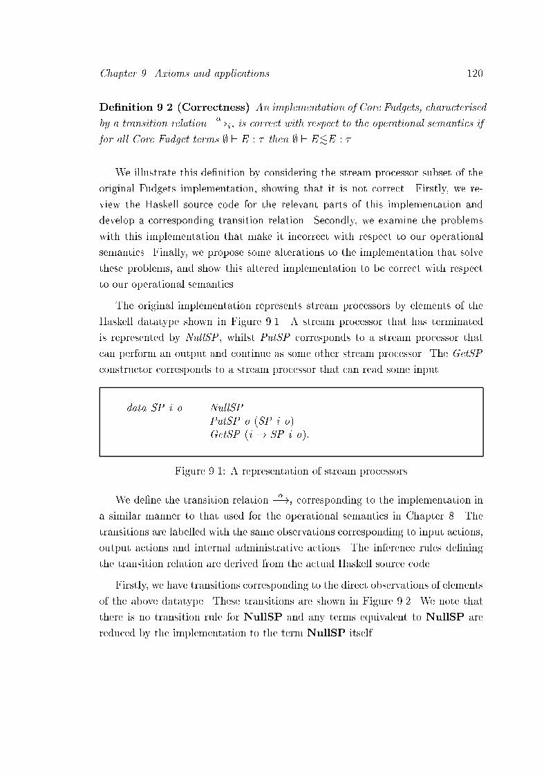
Chapter 9. Axioms and applications 120
De�nition 9.2 (Correctness) An implementation of Core Fudgets, characterised
by a transition relation��!i , is correct with respect to the operational semantics if
for all Core Fudget terms ; ` E : � then ; ` E<�E : � .
We illustrate this de�nition by considering the stream processor subset of the
original Fudgets implementation, showing that it is not correct. Firstly, we re-
view the Haskell source code for the relevant parts of this implementation and
develop a corresponding transition relation. Secondly, we examine the problems
with this implementation that make it incorrect with respect to our operational
semantics. Finally, we propose some alterations to the implementation that solve
these problems, and show this altered implementation to be correct with respect
to our operational semantics.
The original implementation represents stream processors by elements of the
Haskell datatype shown in Figure 9.1. A stream processor that has terminated
is represented by NullSP , whilst PutSP corresponds to a stream processor that
can perform an output and continue as some other stream processor. The GetSP
constructor corresponds to a stream processor that can read some input.
data SP i o = NullSPj PutSP o (SP i o)j GetSP (i ! SP i o):
Figure 9.1: A representation of stream processors
We de�ne the transition relation��!i corresponding to the implementation in
a similar manner to that used for the operational semantics in Chapter 8. The
transitions are labelled with the same observations corresponding to input actions,
output actions and internal administrative actions. The inference rules de�ning
the transition relation are derived from the actual Haskell source code.
Firstly, we have transitions corresponding to the direct observations of elements
of the above datatype. These transitions are shown in Figure 9.2. We note that
there is no transition rule for NullSP and any terms equivalent to NullSP are
reduced by the implementation to the term NullSP itself.

Chapter 9. Axioms and applications 121
(Inpi1)� `?F : �
� ` GetSP E : SP � � 0?F�!i E F
(Out i) � ` PutSP E F : SP � � 0!E�!i F
Figure 9.2: Atomic transitions
Next, we consider serial composition which uses a demand driven approach,
only reducing the right hand side of the serial composition whenever the left hand
side requires some input to continue. The Haskell de�nition in Figure 9.3 imple-
ments serial composition.
(>==<) :: SP m o ! SP i m ! SP i oNullSP >==< f = NullSPPutSP x k >==< f = PutSP x (k >==< f )GetSP f >==< NullSP = NullSPGetSP f >==< PutSP x k = f x >==< kGetSP f >==< GetSP g = GetSP (nx ! GetSP f >==< g x )
Figure 9.3: The implementation of serial composition
The corresponding transition rules for serial composition are derived from the
Haskell de�nition. We must be careful to maintain the semantics of Haskell pattern
matching in these rules. This usually requires some extra transition rules to reduce
arguments to a normal form of either NullSP, GetSP, or PutSP. The rules for
serial composition are shown in Figure 9.4, with (Ser i6) and (Ser i7) reducing the
left hand and right hand side of a serial composition to their normal forms.
As an example of the derivation of a transition rule from the Haskell source
code, we consider the second line of the Haskell de�nition of serial composition.
The corresponding transition rule, (Ser i2), has a hypothesis to ensure that the left
hand side of the serial composition can perform an output action. The conclusion of
the transition rule states that if this hypothesis is valid then the serial composition
can itself perform the same output action. This derivation process captures the
determinancy of the Haskell de�nitions in the corresponding transition rules.

Chapter 9. Axioms and applications 122
(Ser i1) � ` NullSP>==< F : SP � � 0��!i NullSP
(Ser i2)� ` E : SP � 0 � 00
!G�!i E
0
� ` E >==< F : SP � � 00!G�!i E
0 >==< F
(Ser i3)� ` E : SP � 0 � 00
?G�!i E
0
� ` E >==<NullSP : SP � � 00��!i NullSP
(Ser i4)� ` E : SP � 0 � 00
?G�!i E
0 � ` F : SP � � 0!G�!i F
0
� ` E >==< F : SP � � 00��!i E
0 >==< F 0
(Ser i5)� ` E : SP � 0 � 00
?G�!i E
0 � ` F : SP � � 0?H�!i F
0
� ` E >==< F : SP � � 00?H�!i E >==< F 0
(Ser i6)� ` E : SP � 0 � 00
��!i E
0
� ` E >==< F : SP � � 00��!i E
0 >==< F
(Ser i7)� ` E : SP � 0 � 00
?G�!i E
0 � ` F : SP � � 0��!i F
0
� ` E >==< F : SP � � 00��!i E >==< F 0
Figure 9.4: Transition rules for serial composition

Chapter 9. Axioms and applications 123
The implementation of parallel composition is shown in Figure 9.5. We note
that the stream processor on the left hand side of the parallel composition is
examined �rst, and thus if this stream processor continually produces output then
the stream processor on the right hand side will never have a chance to execute.
This implementation is unfair due to the elimination of nondeterminism by simply
choosing to always bias towards one of the branches of a parallel composition.
(>�<) :: SP i o ! SP i o ! SP i oNullSP >�< f = fe >�< NullSP = ePutSP x k >�< f = PutSP x (k >�< f )e >�< PutSP x k = PutSP x (e >�< k)GetSP f >�< GetSP g = GetSP (nx ! f x >�< g x )
Figure 9.5: Parallel composition
The transition rules corresponding to this implementation of parallel compo-
sition are listed in Figure 9.6. The order of the lines in the Haskell de�nition is
important. For example, in the second line e cannot beNullSP. These constraints
are captured in the transition rules, with (Par i4), (Pari5) and (Par i6) reducing the
left and right sides of a parallel composition to their normal forms in the same
manner as the Haskell de�nition.
The feed construct is implemented by the source code shown in Figure 9.7. The
�rst line of the de�nition states that feeding a term into NullSP is equivalent to
NullSP. Feeding a term into a PutSP construct involves moving the feed into
the continuation of the PutSP construct. Finally, feeding a term into a GetSP
construct results in applying the function body of the GetSP construct to the
term being fed. The corresponding transition rules for the feed construct are listed
in Figure 9.8. In this case there is one transition rule for each line of the Haskell
de�nition, and also an extra transition rule that reduces the stream processor
argument to normal form.
The de�nition of the feedback construct given by Carlsson and Hallgren [CH98]
includes the use of auxiliary functions modelling �rst-in �rst-out queues. These
can be represented by the use of the feed construct directly as shown in Figure 9.9,
with the corresponding transition rules in Figure 9.10.

Chapter 9. Axioms and applications 124
(Par i1) � ` NullSP>�< E : SP � � 0��!i E
(Par i2)� ` E : SP � � 0
��!i E
0
� ` E >�<NullSP : SP � � 0��!i E
0 � 6= �
(Par i3)� ` E : SP � � 0
!G�!i E
0 � ` F : SP � � 0��!i F
0
� ` E >�< F : SP � � 0!G�!i E
0 >�< F� 6= �
(Par i4)� ` E : SP � � 0
��!i E
0
� ` E >�< F : SP � � 0��!i E
0 >�< F
(Par i5)� ` E : SP � � 0
?G�!i E
0 � ` F : SP � � 0��!i F
0
� ` E >�< F : SP � � 0��!i E >�< F 0
(Par i6)� ` E : SP � � 0
!G�!i E
0 � ` F : SP � � 0��!i F
0
� ` E >�< F : SP � � 0��!i E >�< F 0
(Par i7)� ` E : SP � � 0
?G�!i E
0 � ` F : SP � � 0!H�!i F
0
� ` E >�< F : SP � � 0!H�!i E >�< F 0
(Par i8)� ` E : SP � � 0
?G�!i E
0 � ` F : SP � � 0?G�!i F
0
� ` E >�< F : SP � � 0?G�!i E
0 >�< F 0
Figure 9.6: Transition rules for parallel composition

Chapter 9. Axioms and applications 125
feedSP :: i ! SP i o ! SP i ofeedSP x NullSP = NullSPfeedSP x (PutSP y k) = PutSP y (feedSP x k)feedSP x (GetSP f ) = f x
Figure 9.7: The implementation of feed
(Feed i1) � ` NullSP� E : SP � � 0��!i NullSP
(Feed i2)� ` E : SP � � 0
!G�!i E
0
� ` E � F : SP � � 0!G�!i E
0 � F
(Feed i3)� ` E : SP � � 0
?F�!i E
0
� ` E � F : SP � � 0��!i E
0
(Feed i4)� ` E : SP � � 0
��!i E
0
� ` E � F : SP � � 0��!i E
0 � F
Figure 9.8: Transition rules for feed
The dynamic stream processor construct is not implemented in the original
Fudgets implementation. Instead, a similar construct is available at the Fudget
level. However, it is straightforward to write a corresponding de�nition for stream
processors, as shown in Figure 9.11. This implementation will produce output in
preference to reading any input, including input indicating that the current stream
processor should be replaced. The corresponding transition rules are shown in
Figure 9.12.
We also need to consider transition rules for the basic computational mecha-
nisms of the language, in this case we have rules for the call-by-name reduction
mechanism of Haskell. Similarly, transition rules are required for literals and their
corresponding constructs such as addition, and case analysis of binary sums. These
transitions rules will be identical to those speci�ed in the operational semantics in
Chapter 8, and so we do not present them again.

Chapter 9. Axioms and applications 126
loopSP :: SP io io ! SP io ioloopSP NullSP = NullSPloopSP (PutSP x k) = PutSP x (loopSP (feedSP x k))loopSP (GetSP f ) = GetSP (nx ! loopSP (f x ))
Figure 9.9: The implementation of feedback
(Loopi1) � ` LoopSP NullSP : SP � ���!i NullSP
(Loopi2)� ` E : SP � �
!G�!i E
0
� ` LoopSP E : SP � �!G�!i LoopSP (E 0 � G)
(Loopi3)� ` E : SP � �
?G�!i E
0
� ` LoopSP E : SP � �?G�!i LoopSP E 0
(Loopi4)� ` E : SP � �
��!i E
0
� ` LoopSP E : SP � ���!i LoopSP E 0
Figure 9.10: Transition rules for feedback
dynSP :: SP (Either (SP i o) i) o! SP (Either (SP i o) i) o
dynSP NullSP = GetSP (nx ! case x ofLeft f ! dynSP fRight ! dynSP NullSP)
dynSP (PutSP x k) = PutSP x (dynSP k)dynSP (GetSP f ) = GetSP (nx ! case x of
Left g ! dynSP gRight x ! dynSP (f x ))
Figure 9.11: The implementation of dynamic stream processors

Chapter 9. Axioms and applications 127
(Dyn i1) � ` DynSP NullSP : SP (SP � � 0 + �) � 0
?Right E�! i DynSP NullSP
(Dyn i2)� ` E : SP � � 0
!F�!i E
0
� ` DynSP E : SP (SP � � 0 + �) � 0!F�!i DynSP E 0
(Dyn i3)� ` E : SP � � 0
?F�!i E
0
� ` DynSP E : SP (SP � � 0 + �) � 0?Left F�! i DynSP F
(Dyn i4)
� ` E : SP � � 0?F�!i E
0
� ` DynSP E : SP (SP � � 0 + �) � 0?Right F�! i DynSP E 0
(Dyn i5)� ` E : SP � � 0
��!i E
0
� ` DynSP E : SP (SP � � 0 + �) � 0��!i DynSP E 0
(Dyn i6)
� ` F : SP � � 0 + ���!i F
0
� ` DynSP E : SP (SP � � 0 + �) � 0?F 0
�!i E0
� ` DynSP E : SP (SP � � 0 + �) � 0?F�!i E
0
Figure 9.12: Transition rules for dynamic stream processors

Chapter 9. Axioms and applications 128
We now proceed to consider if this implementation is correct with respect to
De�nition 9.2. In fact we �nd that it is not correct due to two separate problems:
� The �rst problem is evident if we consider a serial composition of NullSP
and some other stream processor. If we let the other stream processor be
GetSP E then De�nition 9.2 implies that the following diagram is valid:
; ` NullSP>==<GetSP E <� NullSP>==<GetSP E : SP � � 0
; ` NullSP
�
?i<� NullSP>==<GetSP E : SP � � 0
�
wwwwwwwwwww b�
Although we have a matching weak transition, this also implies that we
have ; ` NullSP <� NullSP >==< GetSP E : SP � � 0. This is not
the case because NullSP 6!i yet the other residual term has the transition
; ` NullSP >==< GetSP E : SP � � 0?F�! NullSP >==< E F , and
thus the termination-preserving property of <� is not met. A similar problem
occurs if the right hand side of the serial composition is a stream processor
that can perform some output.
� The second problem is with the dynamic stream processor construct,DynSP.
Considering the term DynSP NullSP then De�nition 9.2 requires that the
following diagram is valid for some term F and action �:
; ` DynSP NullSP <� DynSP NullSP : SP (SP � � 0 + �) � 0
; ` DynSP NullSP
?Right E
?i<� F : SP (SP � � 0 + �) � 0
�
wwwwwwwwwww b�
However, the operational semantics from Chapter 8 does not associate a
transition with the term DynSP NullSP, and thus the only choice for F
is DynSP NullSP yielding the re exive transition where � = �. Unfor-
tunately, this does not satisfy the de�nition of implementation correctness
because the actions ?Right E and � do not match.
The �rst problem can be corrected by modifying the de�nition of serial com-
position of stream processors as shown in Figure 9.13. This involves the addition

Chapter 9. Axioms and applications 129
of the �rst two lines which now allow input and output on the right-hand side of a
serial composition when the left-hand side stream processor has terminated. The
transition relation,��!i , is modi�ed by replacing the (Ser i1) rule with the rules in
Figure 9.14.
(>==<) :: SP m o ! SP i m ! SP i oNullSP >==< GetSP g = GetSP (nx ! NullSP >==< g x )NullSP >==< PutSP x k = NullSP >==< kNullSP >==< f = NullSPPutSP x k >==< f = PutSP x (k >==< f )GetSP f >==< NullSP = NullSPGetSP f >==< PutSP x k = f x >==< kGetSP f >==< GetSP g = GetSP (nx ! GetSP f >==< g x )
Figure 9.13: The modi�ed implementation of serial composition
(Ser i1) � ` NullSP>==<NullSP : SP � � 0��!i NullSP
(Ser i8)� ` F : SP � � 0
��!i F
0
� ` NullSP>==< F : SP � � 00��!i NullSP>==< F 0 � 6=!G
(Ser i9)� ` F : SP � � 0
!G�!i F
0
� ` NullSP>==< F : SP � � 00��!i NullSP>==< F 0
Figure 9.14: New serial composition transition rules
The second problem can be solved by altering the implementation such that
the term DynSP NullSP has no transition. This corresponds to eliminating the
third line of the Haskell de�nition for dynSP , and its associated transition rule
(Dyn i1). This change can be justi�ed because if one wants the behaviour that the
(Dyn i1) transition rule yields then the following Haskell code can be used instead
of DynSP NullSP:
dynNullSP = dynSP ignoreSP
where ignoreSP = GetSP (n ! ignoreSP)
Before showing this altered implementation to be correct according to De�ni-
tion 9.2, we �rst prove an auxiliary lemma regarding input transitions:

Chapter 9. Axioms and applications 130
Lemma 9.1 If � ` E : �?F�!i E 0 then the only possible transition under the
operational semantics is by an input action, or that � ` E : � 6��! and � ` E :
� 6!G�!.
Proof. By induction on the derivation of the transition � ` E : �?F�!i E
0. We
examine two of the cases with the others following in a similar manner:
Case (Inpi1). We have the derivation:
� `?F : �
� ` GetSP E1 : SP � � 0?F�!i E1 F
The term � ` GetSP E1 : SP � � 0 can only make transitions labelled by
input actions under the operational semantics.
Case (Ser i8). We have the derivation:
� ` E1 : SP � � 0?F�!i E2
� ` NullSP>==< E1 : SP � � 00?F�!i NullSP>==< E2
By induction the only possible transition of the term � ` E1 : SP � � 0 under
the operational semantics is via an input action. From the (Ser1) transition
rule then the term � ` NullSP>==< E1 : SP � � 00 can also only perform
a transition via an input action.
The concept of simulation up to can be adapted to correctness simulations and
is useful in simplifying the proof of correctness of an implementation. Note that
S �h denotes the relational composition of S and �h :
De�nition 9.3 (Correctness simulation up to �h) R is a correctness simu-
lation up to �h if it is a closed type-indexed family of relations that are structure-
preserving and ; ` ERF : � implies:
� if ; ` E : ���!i E
0 then 9F 0; �0:; ` F : �b�0
=) F 0 and ; ` E 0R �h F 0 : �
and ; ` �Ra�0 : � 0;
� if ; ` E : � 6!i then 9F0:; ` F : � =) F 0 6!.

Chapter 9. Axioms and applications 131
Lemma 9.2 If S is a correctness simulation up to �h then the relational compo-
sition S �h is also a correctness simulation.
Proof. Let ; ` ES �h F : � and ; ` E : ���!i E
0. It is enough to show that we
can complete the following diagram:
; ` E S �h F : �
where
�(S �h)a�0
; ` E 0
�
?iS �h F 0 : �
�
wwwwwwwwwwwwc�0
To do this, we �rst note that for some F1 then ; ` ESF1 : � and ; ` F1 �h F : � .
Thus we can complete the following two diagrams in sequence, from left to right,
knowing that S is a correctness simulation up to �h :
; ` E S F1 : � ; ` F1 �h F : �
where
�Sa�0
where
�0�h a�00
; ` E 0
�
?iS �h F 0
1
�
wwwwwwwwwwwc�0
; ` F 01
c�0
�
wwwwwwwwwww�h F 0 : �
�
wwwwwwwwwwwwc�00
Composing these, using the transitivity of �h , we easily obtain the required diagram.
A similar argument also holds for the termination property, and it is straightfor-
ward to show the relational composition of two structure-preserving type-indexed
relations to also be structure-preserving.
Lemma 9.3 If S is a correctness simulation up to �h then S � <�.
Proof. Since by lemma 9.2, S �h is a correctness simulation then S �h� <�. But
since the identity relation Id = f(E ;E ) j � ` E �h E : �g is contained in weak
higher-order bisimulation, Id ��h , then we have that S � S �h and can conclude
that S � <� as required.
This lemma is important, because to show ; ` E<�F : � we only need to �nd a
correctness simulation up to �h containing the pair (E ;F ). Using this technique
we can now proceed to show the altered implementation to be correct according
to De�nition 9.2.

Chapter 9. Axioms and applications 132
Theorem 9.5 (Correctness) The implementation of Core Fudgets characterised
by the transition relation��!i is correct with respect to the operational semantics.
Proof. Let the relation S be de�ned as:
S = f(E ;E ) j ; ` E : �g
We proceed by showing this relation to be a correctness simulation up to �h , and
thus ; ` E<�E : � as required. Firstly, it is straightforward to show this relation
to be structure-preserving. Next we show it satis�es the transfer properties for a
correctness simulation up to �h by proceeding by induction on the derivation of the
transition ; ` E : ���!i E
0. We we illustrate the proof by considering a number
of the cases:
Case (Inpi1). We have the derivation:
; `?F : �
; ` GetSP E1 : SP � � 0?F�!i E1 F
By using the (Inp1) transition rule we can derive a matching transition,
; ` GetSP E1 : SP � � 0c?F=) E1 F and ; ` E1 FS �h E1 F : SP � � 0
as required.
Case (Out i). We have the derivation:
; ` PutSP E1 E2 : SP � � 0!E1�!i E2
By using the (Out) transition rule we can derive a matching transition,
; ` PutSP E1 E2 : SP � � 0c!E1=) E2 and ; ` E2S �h E2 : SP � � 0 as
required.
Case (Ser i1). We have the derivation:
; ` NullSP>==<NullSP : SP � � 0��!i NullSP
The only possible matching transition is due to the re exivity of =) giving
; ` NullSP>==<NullSP : SP � � 0b�
=) NullSP>==< NullSP. Since
both NullSP and NullSP>==<NullSP do not have any transitions then

Chapter 9. Axioms and applications 133
; ` NullSP �h NullSP >==< NullSP : SP � � 0 and thus we have ; `
NullSPS �h NullSP>==<NullSP : SP � � 0 as required.
Case (Ser i2). We have the derivation:
; ` E1 : SP � 0 � 00!G�!i E
01
; ` E1 >==< E2 : SP � � 00!G�!i E
01 >==< E2
By induction there is some E 001 such that ; ` E1 : SP � 0 � 00
c!G0
=) E 001 , where
; ` E 01S �
h E 001 : SP � 0 � 00, and ; ` G(S �h)
aG 0 : � 00. Using the (Ser2)
transition rule we derive that ; ` E1 >==< E2 : SP � � 00c!G0
=) E 001 >==< E2.
Also since ; ` E 01S �
h E 001 : SP � 0 � 00 then ; ` E 0
1 �h E 00
1 : SP � 0 � 00.
Finally since �h is preserved by serial composition then we also have ; `
E 01 >==< E2S �h E 00
1 >==< E2 : SP � � 00 as required.
Case (Ser i3). We have the derivation:
; ` E1 : SP � 0 � 00?G�!i E
01
; ` E1 >==<NullSP : SP � � 00��!i NullSP
We have a matching weak transition due to the re exivity of =) giving
; ` E1 >==< NullSP : SP � � 00 =) E1 >==< NullSP. Since we have
; ` E1 : SP � 0 � 00?G�!i E
01 then by Lemma 9.1 the only possible transitions
of E1 under the operational semantics are due to input actions. This allows
us to show that ; ` NullSP �h E1 >==<NullSP : SP � � 00. From this we
obtain ; ` NullSPS �h E1 >==<NullSP : SP � � 00 as required.
The other cases follow in a similar manner.
Finally, we must consider the termination condition and show that for all Core
Fudget terms if ; ` E : � 6!i then there is some E 0 such that ; ` E : � =) E 0 6!.
For our particular implementation, we can show that if ; ` E : � 6!i then it must
be that E = NullSP and thus the termination preserving property follows trivially.
The proof proceeds by induction on the structure of E:
Case E = GetSP E 0. The (Inpi1) rule yields a transition for E.
Case E = PutSP E 0 E 00. The (Out i) rule yields a transition for E.

Chapter 9. Axioms and applications 134
Case E = NullSP. There are no transitions for this term as required.
Case E = E 0 >==< E 00. We consider the possibilities for E 0 and E 00 in the fol-
lowing table, showing that E always has a transition. The entries in the table
correspond to the transition rule that is applicable in each case:
E 0 >==< E 00 E 00 6!i E 00 ��!i E 00 ?F
�!i E 00 !F�!i
E 0 6!i (Ser i1) (Ser i8) (Ser i8) (Ser i9)
E 0 ��!i (Ser i6) (Ser i6) (Ser i6) (Ser i6)
E 0 ?G�!i (Ser i3) (Ser i7) (Ser i5) (Ser i4)
E 0 !G�!i (Ser i2) (Ser i2) (Ser i2) (Ser i2)
For the �rst row and column induction allows us to assume that E 0 = NullSP
and E 00 = NullSP, respectively. For the third row and fourth column it is
su�cient to consider only the cases when G = F.
Case E = E 0 >�< E 00. We consider the possibilities for E 0 and E 00 in the follow-
ing table, showing that E always has a transition. The entries in the table
correspond to the transition rule that is applicable in each case:
E 0 >�< E 00 E 00 6!i E 00 ��!i E 00 ?F
�!i E 00 !F�!i
E 0 6!i (Par i1) (Par i1) (Par i1) (Par i1)
E 0 ��!i (Par i4) (Par i4) (Par i4) (Par i4)
E 0 ?G�!i (Par i2) (Par i5) (Par i8) (Par i7)
E 0 !G�!i (Par i2) (Par i6) (Par i3) (Par i3)
For the �rst row and column induction allows us to assume that E 0 = NullSP
and E 00 = NullSP, respectively. It is su�cient to consider only the case when
G = F for the entry in the third row and third column.
Case E = E 0 � E 00. It is su�cient to consider the possible transitions of E 0 alone,
and we detail the transitions for these cases in the following table:
E 0 � E 00 E 0 6!i E 0 ��!i E 0 ?G
�!i E 0 !G�!i
(Feed i1) (Feed i4) (Feed i3) (Feed i2)
For the �rst column, induction allows us to assume that E 0 = NullSP.
The remaining cases all follow in a similar manner.

Chapter 10
Summary and further work
In this dissertation we have shown how a theory of the Fudgets system can be
developed using ideas from concurrency theory. Firstly, we identi�ed a core lan-
guage underlying the Fudgets system, and next we developed two separate formal
semantics for this language. Finally, we illustrated the application of such theories
by developing equational rules and checking the correctness of implementations.
The �rst formal semantics we considered assigns meanings to programs by a
translation into the �-calculus. There are two main advantages with using the
�-calculus as a metalanguage. Firstly, there has been a great deal of work on the
theory of the �-calculus and we can leverage this work to indirectly give a theory to
Fudget programs. Secondly, the translation of Fudget programs into the �-calculus
can be used as a reference implementation of the Fudgets system. However, the �-
calculus is quite a low-level language and this makes proofs about Fudget programs
long and tedious. This leads to the intuition behind the semantics of various core
language constructs being lost in the �-calculus translations.
The second formal semantics we developed associates meanings to programs
by operational transitions. This approach is much more direct than the �rst, but
required a new theory to be developed. Various equivalences based on bisimulation
were examined and weak higher-order bisimulation was chosen as an appropriate
equivalence. This was shown to be a congruence, which is an important property
for the equivalence because it allows it to be used as the basis of an equational
theory where a subterm can be replaced by an equivalent subterm.
Finally, we considered applications of the formal semantics, speci�cally the sec-
ond operational semantics. A set of equational rules were developed that are useful
135

Chapter 10. Summary and further work 136
for reasoning about Fudget programs without recourse to the complex machinery of
bisimulation. A notion of implementation correctness was de�ned with respect to
the operational semantics, and the original implementation of the Fudgets system
was shown to be correct modulo some minor modi�cations.
10.1 Further work
We conclude the dissertation by describing possible future work, outlining prelim-
inary ideas in each case.
Semantics of feedback: In Section 7.4 we discussed two possibilities for the
semantics of the merge operation on the input side of the feedback construct
LoopSP. The denotational semantics of Chapter 6 gives this merge operation
a nondeterministic semantics, whilst in the operational semantics it has a deter-
ministic semantics. Ideally, we would have liked to give the merge operation a
nondeterministic semantics in the operational semantics. However, it is not obvi-
ous how to modify the (Loop2) transition rule from Chapter 8 such that this is the
case. This would be an interesting area for further work.
Equivalence of semantics: Chapter 6 describes a denotational semantics for
the Core Fudgets language, whilst Chapter 8 presents an operational semantics.
An obvious question is how these two semantics relate to one another. However,
to answer this question the feed construct described in Chapter 8 must be given
an encoding in terms of the �-calculus. Comparing the two semantics is really
an issue of comparing two operational semantics, the �rst being that induced by
the denotational semantics and the operational semantics of the �-calculus. The
second is simply the direct operational semantics of Core Fudgets from Chapter 8.
Comparison to other systems: Now that we have developed some formal
theories for the Fudgets system, another possible application would be to use
them to compare the Fudgets system to other graphical development systems.
In particular, since we have a �-calculus semantics for the Fudgets system then
this may be useful in comparing the Fudgets system to the Haggis system [FJ95].
This is because the Haggis system is written in Concurrent Haskell, for which

Chapter 10. Summary and further work 137
a formal semantics has been developed based on the �-calculus thus inducing a
formal semantics for the Haggis system itself. In particular, this comparison may
lead to some formal quanti�cation of the relative expressiveness of the two systems.
Deriving implementations: We show in Chapter 9 how the operational se-
mantics for Core Fudgets can be used to verify the correctness of implementations
of the language. Another application of the semantics, that is closely related to
correctness, could be to derive a correct implementation. This could be achieved
by using a concurrent variant of Haskell such as Concurrent Haskell. This would
enable the operational semantics to be encoded almost directly into the functional
language. However, if there are no concurrent constructs in the target language
then this would be more di�cult. The nondeterminism of constructs such as par-
allel composition of stream processors could be eliminated by arbitrarily biasing
to either the left or right stream processor in the composition. A notion of fairness
would ideally need to be introduced in order to check whether such implementa-
tions were reasonable.
Lack of identities for serial composition: The equational rules we developed
in Chapter 9 did not include standard identity rules for serial composition. Intu-
itively, we would expect the identity stream processor to be the identity for serial
composition, but we showed this not to be the case. One solution is to adopt a
demand driven approach as done in the original implementation of the Fudgets
system. An alternative approach may be to extend the operational semantics with
the (Inp2) inference rule as discussed in Section 9.1:
(Inp2)� ` F : �
� ` E : SP � � 0?F�! E � F
The identity stream processor turns out to be an identity for serial composition
under this extended semantics. However, some of the technical results we have
developed need to be veri�ed for this extended system, although it is straightfor-
ward to verify that the main result { the proof of congruence for weak higher-order
bisimulation { still holds with this new transition rule. An investigation into the
properties of this extended system is also a useful direction for further work, and
we would hope that all of the equational rules from Chapter 9 still hold.

Appendix A
Proof of theorem 8.1
In this appendix we show that higher-order weak bisimulation, �, is a congru-
ence for the Core Fudgets language, and is thus preserved by all of the languages
constructs. The proof proceeds by a typed reworking of Howe's method [How89].
A.1 Overview of the proof
The proof of congruence follows a technique proposed by Howe [How89] which
was �rst used in the context of applicative simulation equivalences for the lazy
�-calculus. The core of this method involves the de�nition of a closure operator,
( )�, which by de�nition is a congruence. Three steps are then required to obtain
the desired congruence result:
� Establishing standard properties. A set of standard properties are shown
to be valid for the closure operator ( )�. These properties are used in the
remaining two steps of the proof.
� Proving a strengthened simulation property. This is the main step of the
proof, and involves showing the relation �� to satisfy a strengthened form of
the properties required for a relation to be a weak higher-order simulation.
� Concluding the proof. The relation �� is shown to be a weak higher-order
bisimulation using an observation of Howe's regarding the closure operator
( )�. Finally, a set inclusion argument is used to show �� to be equal to ��,
and hence �� is a congruence.
138

Appendix A. Proof of theorem 8.1 139
A.2 Compatible re�nement
Howe's method for proving a bisimulation relation to be a congruence makes use of
an alternative characterisation of congruence based upon the concept of compatible
re�nement. The compatible re�nement of a relation R relates those expressions
that have the same toplevel syntactic constructor and whose corresponding sub-
terms are related by R. Formally, we de�ne compatible re�nement as:
De�nition A.1 (Compatible re�nement) For an open type-indexed relation R
on Core Fudget terms, we de�ne its compatible re�nement, cR, as the least relationde�ned by the inference rules in Figures A.1 , A.2, and A.3.
(Comp Lit) � ` E cR E : � if E is a literal
(Comp Var) � ` x cR x : �
(Comp Abs)�; x : � ` E R E 0 : � 0
� ` �x :E cR �x :E 0 : � ! � 0
(Comp App)� ` E R E 0 : � ! � 0 � ` F R F 0 : �
� ` E F cR E 0 F 0 : � 0
(Comp Fix )�; x : � ` E R E 0 : �
� ` Fix x :E cR Fix x :E 0 : �
Figure A.1: Compatible re�nement for literals and expressions
An alternative de�nition of congruence to that given in De�nition 8.4 can now be
formulated in terms of compatible re�nement:
De�nition A.2 (Congruence2) A relation R is a precongruence if and only if
it contains its own compatible re�nement, cR � R. A congruence is an equivalence
relation that is a precongruence.

Appendix A. Proof of theorem 8.1 140
(Comp Null) � ` NullSP cRNullSP : SP � � 0
(Comp Get)� ` E R E 0 : � ! SP � � 0
� ` GetSP E cRGetSP E 0 : SP � � 00
(Comp Put)� ` E R E 0 : � 0 � ` F R F 0 : SP � � 0
� ` PutSP E F cRPutSP E 0 F 0 : SP � � 0
(Comp Par)� ` E R E 0 : SP � � 0 � ` F R F 0 : SP � � 0
� ` E >�< F cR E 0 >�< F 0 : SP � � 0
(Comp Ser)� ` E R E 0 : SP � 0 � 00 � ` F R F 0 : SP � � 0
� ` E >==< F cR E 0 >==< F 0 : SP � � 00
(Comp Loop)� ` E R E 0 : SP � �
� ` LoopSP E cR LoopSP E 0 : SP � �
(Comp Dyn)� ` E R E 0 : SP � � 0
� ` DynSP E cRDynSP E 0 : SP (SP � � 0 + �) � 0
(Comp Feed)� ` E R E 0 : SP � � 0 � ` F R F 0 : �
� ` E � F cR E 0 � F 0 : SP � � 0
Figure A.2: Compatible re�nement for stream processors

Appendix A. Proof of theorem 8.1 141
(Comp LInj )� ` E R E 0 : �
� ` Left E cR Left E 0 : � + � 0
(Comp RInj )� ` F R F 0 : � 0
� ` Right F cRRight F 0 : � + � 0
(Comp Case)� ` E R E 0 : � + � 0 � ` F R F 0 : � ! � 00 � ` G RG 0 : � 0 ! � 00
� ` Case E ! F ;G cRCase E 0 ! F 0;G 0 : � 00
(Comp If )� ` E R E 0 : bool � ` F R F 0 : � � ` G R G 0 : �
� ` if E then F else G cR if E 0 then F 0 else G 0 : �
(Comp Add)� ` E R E 0 : num � ` F R F 0 : num
� ` add E F cR add E 0 F 0 : num
(Comp Equal)� ` E R E 0 : num � ` F R F 0 : num
� ` equal E F cR equal E 0 F 0 : bool
Figure A.3: Compatible re�nement for constant functions
Recalling the earlier de�nition of congruence in terms of contexts, we can show
that this is equivalent to our formulation of congruence in terms of compatible
re�nement:
Lemma A.1 The two characterisations of congruence from De�nitions 8.4 and
A.2 are equivalent.
Proof. It is straightforward to show that the inference rules characterising com-
patible re�nement can be derived from (Cong R) and by using the properties of
the relation R, such as re exivity and transitivity. To show that cR � R implies
(Cong R) requires using induction on the derivation of � ` C[�� ] : �0 to show that
if �0 is the list of bound variables in the context C then �;�0 ` ERE 0 : � implies
that � ` C[E ]RC[E 0] : � 0. We consider the case for the GetSP construct:
Case � ` GetSP C 0 : SP � � 0. By induction, the result holds for C 0 and so we
have the derivation � ` C 0[E ]RC 0[E 0] : � ! SP � � 0, and using (Comp Get)
we obtain � ` GetSP C 0[E ] cRGetSP C 0[E 0] : SP � � 0, as required.
The other cases follow in a similar manner.

Appendix A. Proof of theorem 8.1 142
A.3 Compatible closure
The core of Howe's method is the de�nition of a special relation, called the com-
patible closure, which by de�nition is a congruence. The main idea is then to show
that the relation one wishes to prove to be a congruence is equal to the compatible
closure of that relation.
De�nition A.3 (Compatible closure) The compatible closure of a type-indexed
relation, R, is denoted by R� and is de�ned by the following inference rule:
(Cand Def) � ` E dR� E 00 : � � ` E 00 R� E 0 : �� ` E R� E 0 : �
This de�nition is both circular and asymmetric, and it may appear that the cir-
cularity will lead to empty relations, but this is shown not to be the case in the
following lemma. The asymmetry of the de�nition suggests that it may only be
useful for showing non-symmetric relations to be congruences, but this problem
can be overcome by using a recent observation of Howe's, and we will return to
this point in a later section.
Lemma A.2 (Properties of compatible closure) If R is a preorder then its
compatible closure R� satis�es the inference rules listed in Figure A.4.
(Cand Re ) � ` E R� E : �
(Cand Cong) � ` E dR� E 0 : �� ` E R� E 0 : �
(Cand Right) � ` E R� E 00 : � � ` E 00 R� E 0 : �� ` E R� E 0 : �
(Cand Sim) � ` E R� E 0 : �� ` E R� E 0 : �
(Cand Subst)�; x : � ` E R� E 0 : � 0 � ` F R� F 0 : �
� ` E [F=x ]R� E 0[F 0=x ] : � 0
Figure A.4: Properties of compatible closure

Appendix A. Proof of theorem 8.1 143
Proof. We consider the proof of each inference rule separately:
(Cand Re ). By using the re exivity of R, we can use structural induction on E
to show that � ` E R� E : � .
(Cand Cong). By using (Cand Def ), setting E 00 = E 0, and by the re exivity of
R� the result follows.
(Cand Right). From � ` ER�E 00 : � and by using the (Cand Def ) rule there must
be some E 000 such that � ` EdR�E 000 : � and � ` E 000R�E 00 : � . The transitivity
of R� allows us to deduce � ` E 000 R� E 0 : � , and using the (Cand Def ) rule
yields � ` E R� E 0 : � as required.
(Cand Sim). Since R� is re exive by (Cand Re ) then we have that � ` ER�E : �
and combining this with the hypothesis of (Cand Sim), � ` ER�E 0 : � , using
the (Cand Right) rule we obtain � ` E R� E 0 : � as required.
(Cand Subst). The proof proceeds by induction on the structure of the derivation
of �; x : � ` E R� E 0 : � 0. By de�nition from the (Cand Def ) rule there is
some E 00 such that �; x : � ` E dR� E 00 : � 0 and �; x : � ` E 00R� E 0 : � 0. From
the de�nition of R� on open terms we have � ` E 00[F 0=x ]R�E 0[F 0=x ] : � 0. We
proceed by structural analysis of E and show that in each case the judgement
� ` E [F=x ]R� E 00[F 0=x ] : � 0 can be derived:
Case E = GetSP G. From the de�nition of dR� then E 00 = GetSP G 0,
where �; x : � ` GR�G 0 : � 00 ! � 0. By induction we have the derivation
� ` G [F=x ] R� G 0[F 0=x ] : � 00 ! � 0, and so by using the (Comp Get)
rule we obtain that � ` GetSP (G [F=x ])dR� GetSP (G 0[F 0=x ]) : � 0.
The rules of substitution along with the (Cand Cong) rule give us the
required result, � ` (GetSP G)[F=x ]R� (GetSP G 0)[F 0=x ] : � 0.
The other cases follow in a similar manner.
The properties listed in Figure A.4 are standard, and will be required in the
next section to show the equivalence of a relation and its compatible closure. The
(Cand Subst) rule is especially important in the proof technique as it is necessary
in handling the synchronisation cases involving substitution that cause problems
for proof techniques that work for �rst-order calculi.

Appendix A. Proof of theorem 8.1 144
A.4 Congruence of �
We are now in a position to prove the open extension of higher-order weak bisim-
ulation to be a congruence. If we consider the compatible closure of higher-order
weak bisimulation �h �, then by de�nition this is a congruence as it contains its
own compatible re�nement. The result will follow if we can show that �h � � �h �
and �h � � �h �. The �rst of these equations follows directly from the (Cand Sim)
rule, while the second requires further work.
We approach the problem of showing �h� � �h �, by considering the restriction
of �h � to closed terms as captured by the following relation:
S = f(E ;F ) j ; ` E�h �F : �g
First, we show that this relation is structure-preserving:
Lemma A.3 The relation S is structure-preserving.
Proof. There are four cases to consider:
Case ; ` L�h�E : � , where � 2 fbool;numg. From (Cand Def ) there must be
some E 0 such that ; ` Ld�h�E 0 : � where ; ` E 0�h�E : � . However, be-
cause L is a literal then the only rule that can be used to infer the �rst of
these judgements is the (Comp Lit) rule, and thus E 0 = L. Further, from
the de�nition of open extension then we have ; ` E 0�hE : � and as �h
is structure-preserving by de�nition then there must be some M such that
; ` E : � =) M and L = M as required.
Case ; ` Left E�h �F : � + � 0. From the (Cand Def ) rule there is some G such
that ; ` Left E d�h �G : � + � 0 and ; ` G�h �F : � + � 0. By the de�nition of
compatible re�nement then there is some G 0 such that G = Left G 0 where
; ` E�h �G 0 : � . Further, from the de�nition of open extension then we have
that ; ` G�hF : � + � 0 and because �h is structure-preserving then there is
some F 0 such that ; ` F : � + � 0 =) Left F 0 where ; ` G 0�hF 0 : � . Finally,
from the de�nition of open extension this is equivalent to ; ` G 0�h�F 0 : � and
by using (Cand Right) we can thus show that ; ` E�h �F 0 : � as required.

Appendix A. Proof of theorem 8.1 145
Case ; ` Right E�h �F : � + � 0. From the (Cand Def ) rule there is some G such
that ; ` Right E d�h �G : � + � 0 and ; ` G�h �F : � + � 0. By the de�nition
of compatible re�nement then there is some G 0 such that G = Right G 0 and
; ` E�h �G 0 : � 0. Further, from the de�nition of open extension then we have
; ` G�hF : � + � 0 and as �h is structure-preserving then there is some F 0
such that ; ` F : � + � 0 =) Right F 0 where ; ` G 0�hF 0 : � 0. Finally, from
the de�nition of open extension this is equivalent to ; ` G 0�h �F 0 : � 0 and by
using (Cand Right) we can thus show that ; ` E�h �F 0 : � 0 as required.
Case ; ` (�x :E )�h�F : � ! � 0. From (Cand Def ) there must be some G such
that ; ` (�x :e)d�h �G : � ! � 0 where ; ` G�h �F : � ! � 0. From the
(Comp Abs) rule then there must be some G 0 such that G = (�x :G 0) where
x : � ` E�h �G 0 : � 0. Using the (Cand Cong) rule we obtain the derivation
; ` (�x :E )�h�(�x :G 0) : � ! � 0, and from the (Cand Re ) rule we have
y : � ` y�h �y : � . Thus, by using the (Comp App) and (Cand Cong) rules
we can infer that y : � ` (�x :E ) y�h�(�x :G 0) y : � 0. For all ; ` H : �
using the (Cand Re ) rule we can show that ; ` H�h �H : � and thus from
(Cand Subst) we can derive ; ` (�x :E ) H�h �(�x :G 0) H : � 0. Further,
from the de�nition of open extension then ; ` G�hF : � ! � 0 and as �h
is structure-preserving by de�nition then there must be some F 0 such that
; ` F : � ! � 0 =) (�x :F 0), where for all terms ; ` H 0 : � then we have
; ` (�x :G 0) H 0�h(�x :F 0) H 0 : � . The de�nition of open extension allows us
to infer that ; ` (�x :G 0) H 0�h �(�x :F 0) H 0 : � . We can instantiate H 0 to be
H and thus for all terms ; ` H : � then by using (Cand Right) we have that
(�x :E ) H�h�(�x :F 0) H ` � : as required.
We prove some auxiliary lemmas regarding the dynamic stream processor con-
struct that will be required later in the proof:
Lemma A.4 If � ` G : SP � � 0 + � =) G 0 and � ` DynSP E : SP (SP � � 0 +
�) � 0?G0
�! E 0 then � ` DynSP E : SP (SP � � 0 + �) � 0c?G=) E 0.
Proof. By induction on the length of the transition � ` G : SP � � 0 + � =) G 0:
Case Base Case. In this case G = G 0 and so the result follows trivially.

Appendix A. Proof of theorem 8.1 146
Case Inductive Case. There is some G 00 such that � ` G : SP � � 0 + � =) G 0
can be broken into the two separate transitions � ` G : SP � � 0 + � =) G 00
and � ` G 00 : SP � � 0+ ���! G 0. From the second of these transitions along
with � ` DynSP E : SP (SP � � 0+�) � 0?G0
�! E 0 using the (Dyn2) transition
rule we can conclude that � ` DynSP E : SP (SP � � 0+ �) � 0?G00
�! E 0. Now
by induction we can show that � ` DynSP E : SP (SP � � 0 + �) � 0c?G=) E 0
as required.
Lemma A.5 If � ` G : SP � � 0 + � =) G 0 and � ` DynSP E : SP (SP � � 0 +
�) � 0?G0
=) E 0 then � ` DynSP E : SP (SP � � 0 + �) � 0c?G=) E 0.
Proof. From � ` DynSP E : SP (SP � � 0 + �) � 0?G0
=) E 0 then there must be
some E 00 and E 000 such that � ` DynSP E : SP (SP � � 0+ �) � 0 =) E 00, � ` E 00 :
SP (SP � � 0 + �) � 0?G0
�! E 000 and � ` DynSP E 000 : SP (SP � � 0 + �) � 0 =) E 0.
The only possible � transitions for terms of the form DynSP E are due to the
(Dyn1) transition rule, and thus E 00 = DynSP E 0000. Since � ` DynSP E 0000 :
SP (SP � � 0+�) � 0?G0
�! E 000 and � ` G : SP � � 0+� =) G 0 then by Lemma A.4 we
have that � ` DynSP E 0000 : SP (SP � � 0+�) � 0c?G=) E 000. Finally using the (Dyn1)
transition rule we can deduce that � ` DynSP E : SP (SP � � 0 + �) � 0c?G=) E 0as
required.
Next, we show the relation S to satisfy a strengthened set of the transfer prop-
erties required for a relation to be a weak higher-order simulation. The di�erence
in these properties and those required by weak higher-order simulation is in the
treatment of input actions: instead of requiring an input action to be matched
precisely we require there to be matching transitions for all semantically equiva-
lent inputs. This modi�cation to the transfer properties is critical to the success
of showing S to satisfy the transfer properties of weak higher-order simulation.
The properties of weak higher-order simulation are just one instance of these more
general properties.

Appendix A. Proof of theorem 8.1 147
Lemma A.6 The relation S satis�es the following strengthened transfer properties
of weak higher-order simulation where ; ` ESF : � implies:
� if ; ` E : �?G�! E 0 then 8G 0:; ` G �h � G 0 : � 0 implies 9F 0:; ` F : �
c?G0
=) F 0
and ; ` E 0 �h� F 0 : � ;
� if ; ` E : ���! E 0 then 9F 0:; ` F : � =) F 0 and ; ` E 0 �h� F 0 : � ;
� if ; ` E : �!G�! E 0 then 9F 0;G 0:; ` F : �
c!G0
=) F 0 and ; ` E 0 �h � F 0 : � and
; ` G �h � G 0 : � 0.
Proof. By induction on the structure of the derivation of ; ` E��! E 0 : � . Since
; ` E�h �F : � , then from the (Cand Def ) rule we know that there is some H such
that ; ` E d�h� H : � and ; ` H �h � F : � . It is su�cient to show that there are
appropriate transitions of H because if ; ` H : �b�
=) H 0 then from the de�nition
of �h � there must also be a transition ; ` F : �b�0
=) F 0 where ; ` ��h�a�0 : � 00
and ; ` H 0�h�F 0 : � . By using (Cand Right) and (Cand Cong) we can use this
to relate the residual term of the transition of E to F 0 as required:
Case (Inp1). We have the derivation:
; `?G : �
; ` GetSP E1 : SP � � 0?G�! E1 G
From the (Comp Get) rule there is some H1 such that H = GetSP H1, where
; ` E1�h �H1 : � ! SP � � 0. From the (Inp Act) typing rule for actions we
can infer that for all G 0 such that ; ` G �h � G 0 : � then ; `?G 0 : � . Using
this with the (Inp1) transition rule we can infer that for each G 0 then we have
a derivation of the form:
; `?G 0 : �
; ` GetSP H1 : SP � � 0c?G0
=) H1 G0
Finally, because ; ` E1�h�H1 : � ! SP � � 0 and ; ` G�h �G 0 : � then using
(Comp App) and (Cand Cong) we obtain ; ` E1 G�h�H1 G 0 : SP � � 0 as
required.

Appendix A. Proof of theorem 8.1 148
Case (Out). We have the derivation:
; ` PutSP E1 E2 : SP � � 0!E1�! E2
From (Comp Put) there is some H1 and H2 such that H = PutSP H1 H2
where ; ` E1�h �H1 : �0 and ; ` E1�h�H2 : SP � � 0. By the transition rule
(Out) we infer the required derivation ; ` PutSP H1 H2 : SP � � 0!H1=) H2.
Case (Feed1). We have the derivation:
; ` E1 : SP � � 0?E2�! E3
; ` E1 � E2 : SP � � 0��! E3
From the (Comp Feed) rule there is some H1 and H2 such that H = H1 � H2
where ; ` E1�h�H1 : SP � � 0 and ; ` E2�h�H2 : � . By induction for
all G 0 such that ; ` E2�h �G 0 : � then ; ` H1 : SP � � 0c?G0
=) H3 where
; ` E3�h �H3 : SP � � 0. We can instantiate G 0 to be H2 yielding the transition
; ` H1 : SP � � 0d?H2=) H3, and from the (Feed1) transition rule we can infer
; ` H1 � H2 : SP � � 0 =) H3.
Case (Feed2). We have the derivation:
; ` E1 : SP � � 0��! E3
; ` E1 � E2 : SP � � 0��! E3 � E2
where � 2 f�; !Gg. From the (Comp Feed) rule there is some H1 and H2 such
that H = H1 � H2 where ; ` E1�h �H1 : SP � � 0 and ; ` E2�h�H2 : � . We
consider each of the two cases for � in turn:
� � = �, then by induction we have the derivation ; ` H1 : SP � � 0 =) H3
where ; ` E3�h �H3 : SP � � 0. Using the (Feed2) rule with this we can
infer ; ` H1 � H2 : SP � � 0 =) H3 � H2.
� � =!G, then by induction for some G 0 such that ; ` G�h �G 0 : � 0
then ; ` H1 : SP � � 0c!G0
=) H3 where ; ` E3�h�H3 : SP � � 0. Using the
(Feed2) rule with this we can infer ; ` H1 � H2 : SP � � 0c!G0
=) H3 � H2.
Finally, in both cases we can use the (Comp Feed) and (Cand Cong) rules
to obtain ; ` E3 � E2�h �H3 � H2 : SP � � 0 as required.

Appendix A. Proof of theorem 8.1 149
Case (Ser1). We have the derivation:
; ` E2 : SP � � 0��! E3
; ` E1 >==< E2 : SP � � 00��! E1 >==< E3
where � 2 f�; ?Gg. From the (Comp Ser) rule then there is some H1 and
H2 such that H = H1 >==< H2 where ; ` E1�h �H1 : SP � 0 � 00 and ; `
E2�h �H2 : SP � � 0. We consider each of the two cases for � in turn:
� � = �, then by induction we have the derivation ; ` H2 : SP � � 0 =) H3
where ; ` E3�h �H3 : SP � � 0. From the (Ser1) rule we can infer
; ` H1 >==< H2 : SP � � 00 =) H1 >==< H3.
� � =?G, then by induction for all G 0 such that ; ` G�h �G 0 : � then
; ` H2c?G0
=) H3 : SP � � 0 where ; ` E3�h �H3 : SP � � 0. Using the (Ser1)
rule we can thus infer ; ` H1 >==< H2 : SP � � 00c?G0
=) H1 >==< H3.
Finally, in both cases we can use the (Comp Ser) and (Cand Cong) rules to
obtain ; ` E1 >==< E3�h �H1 >==< H3 : SP � � 00 as required.
Case (Ser2). We have the derivation:
; ` E1 : SP � � 0��! E3
; ` E1 >==< E2 : SP � � 00��! E3 >==< E2
where � 2 f�; !Gg. From the (Comp Ser) rule then there is some H1 and
H2 such that H = H1 >==< H2 where ; ` E1�h �H1 : SP � 0 � 00 and ; `
E2�h �H2 : SP � � 0. We consider each of the two cases for � in turn:
� � = �, then by induction we have the derivation ; ` H1 : SP � � 0 =) H3
where ; ` E3�h �H3 : SP � � 0. From the (Ser1) rule we can infer
; ` H1 >==< H2 : SP � � 00 =) H3 >==< H1.
� � =?G, then by induction for all G 0 such that ; ` G�h �G 0 : � then
; ` H1c?G0
=) H3 : SP � � 0 where ; ` E3�h �H3 : SP � � 0. Using the (Ser1)
rule we can thus infer ; ` H1 >==< H2 : SP � � 00c?G0
=) H3 >==< H2.
Finally, in both cases we can use the (Comp Ser) and (Cand Cong) rules to
obtain ; ` E3 >==< E2�h �H3 >==< H2 : SP � � 00 as required.

Appendix A. Proof of theorem 8.1 150
Case (Ser3). We have the derivation:
; ` E2 : SP � � 0!G�! E3
; ` E1 >==< E2 : SP � � 00��! E1 � G >==< E3
From (Comp Ser) there is some H1 and H2 such that H = H1>==<H2 where
; ` E1�h�H1 : SP � 0 � 00 and ; ` E2�h �H2 : SP � � 0. By induction then for
some G 0 such that ; ` G�h �G 0 : � 0 then ; ` H2 : SP � � 0c!G0
=) H3 where
; ` E3�h �H3 : SP � � 0. From the (Ser1) and (Ser3) rules we can thus deduce
the derivation ; ` H1 >==< H2 : SP � � 00 =) H1 � G 0 >==< H3. Since
; ` E1�h�H1 : SP � 0 � 00 and ; ` G�h �G 0 : � 0 then by using (Comp Feed)
and (Cand Cong) we obtain ; ` E1 � G�h �H1 � G 0 : SP � 0 � 00. From
this using the (Comp Ser) and (Cand Cong) rules we obtain the required
derivation ; ` E1 � G >==< E3�h �H1 � G 0 >==< H3 : SP � � 00.
Case (Par1). We have the derivation:
; ` E1 : SP � � 0��! E3
; ` E1 >�< E2 : SP � � 0��! E3 >�< E2
where � 2 f�; !Gg. From (Comp Par) there is some H1 and H2 such that
H = H1 >�< H2 where ; ` E1�h �H1 : SP � � 0 and ; ` E2�
h �H2 : SP � � 0.
We consider each of the two cases for � in turn:
� � = �, then by induction we have the derivation ; ` H1 : SP � � 0 =) H3
where ; ` E3�h�H3 : SP � � 0. From the (Par1) rule we obtain the
derivation ; ` H1 >�< H2 : SP � � 0 =) H3 >�< H2.
� � =!G, then by induction for some G 0 such that ; ` G�h �G 0 : � 0 then
; ` H1 : SP � � 0c!G0
=) H3 where ; ` E3�h�H3 : SP � � 0. Using this with
the (Par1) we get ; ` H1 >�< H2 : SP � � 0c!G0
=) H3 >�< H2.
Finally, because ; ` E3�h �H3 : SP � � 0 and ; ` E2�h �H2 : SP � � 0 in both
cases then we can use the (Comp Par) and (Cand Cong) rules to obtain
; ` E3 >�< E2�h �H3 >�< H2 : SP � � 0 as required.

Appendix A. Proof of theorem 8.1 151
Case (Par2). We have the derivation:
; ` E2 : SP � � 0��! E3
; ` E1 >�< E2 : SP � � 0��! E1 >�< E3
where � 2 f�; !Gg. From (Comp Par) there is some H1 and H2 such that
H = H1 >�< H2 where ; ` E1�h �H1 : SP � � 0 and ; ` E2�h �H2 : SP � � 0.
We consider each of the two cases for � in turn:
� � = �, then by induction we have the derivation ; ` H2 : SP � � 0 =) H3
where ; ` E3�h�H3 : SP � � 0. From the (Par1) rule we obtain the
derivation ; ` H1 >�< H2 : SP � � 0 =) H1 >�< H3.
� � =!G, then by induction for some G 0 such that ; ` G�h �G 0 : � 0 then
; ` H2 : SP � � 0c!G0
=) H3 where ; ` E3�h�H3 : SP � � 0. Using this with
the (Par1) we get ; ` H1 >�< H2 : SP � � 0c!G0
=) H1 >�< H3.
Finally, because ; ` E1�h �H1 : SP � � 0 and ; ` E3�h �H3 : SP � � 0 in both
cases then we can use the (Comp Par) and (Cand Cong) rules to obtain
; ` E1 >�< E3�h �H1 >�< H3 : SP � � 0 as required.
Case (Par3). We have the derivation:
; ` E1 : SP � � 0?G�! E3
; ` E1 >�< E2 : SP � � 0?G�! E3 >�< (E2 � G)
From (Comp Par) there is some H1 and H2 such that H = H1>�<H2 where
; ` E1�h �H1 : SP � � 0 and ; ` E2�h �H2 : SP � � 0. By induction then
for all G 0 such that ; ` G�h �G 0 : � then ; ` H1 : SP � � 0c?G0
=) H3 where
; ` E3�h �H3 : SP � � 0. Using this along with the (Par1) and (Par3) rules
we can infer that ; ` H1 >�< H2 : SP � � 0c?G0
=) H3 >�< (H2 � G 0). We
can infer ; ` E2 � G�h �H2 � G 0 : SP � � 0 from the (Comp Feed) and
(Cand Cong) rules. Finally, from (Comp Par) and (Cand Cong) we obtain
; ` E3 >�< (E2 � G)�h �H3 >�< (H2 � G 0) : SP � � 0 as required.

Appendix A. Proof of theorem 8.1 152
Case (Par4). We have the derivation:
; ` E2 : SP � � 0?G�! E3
; ` E1 >�< E2 : SP � � 0?G�! (E1 � G) >�< E3
From (Comp Par) there is some H1 and H2 such that H = H1>�<H2 where
; ` E1�h �H1 : SP � � 0 and ; ` E2�h �H2 : SP � � 0. By induction then
for all G 0 such that ; ` G�h �G 0 : � then ; ` H2 : SP � � 0c?G0
=) H3 where
; ` E3�h �H3 : SP � � 0. Using this with (Par1) and (Par4) we obtain the
derivation ; ` H1>�<H2 : SP � � 0c?G0
=) (H1 � G 0)>�<H3. We can show that
; ` E1 � G�h �H1 � G 0 : SP � � 0 using the (Comp Feed) and (Cand Cong)
rules. Finally, using this with the (Comp Par) and (Cand Cong) rules we
obtain ; ` (E1 � G)>�< E3�h �(H1 � G 0)>�< H3 : SP � � 0 as required.
Case (Loop1). We have the derivation:
; ` E1 : SP � ���! E2
; ` LoopSP E1 : SP � ���! LoopSP E2
where � 2 f�; ?Gg. From the (Comp Loop) rule there is some H1 such that
H = LoopSP H1 where ; ` E1�h�H1 : SP � � . We consider each of the
two cases for � in turn:
� � = �, then by induction we have the derivation ; ` H1 : SP � � =) H2
where ; ` E2�h �H2 : SP � � . From the (Loop1) rule we can thus infer
the derivation ; ` LoopSP H1 : SP � � =) LoopSP H2.
� � =?G, then by induction for all G 0 such that ; ` G�h �G 0 : � then
; ` H1 : SP � �c?G0
=) H2 where ; ` E2�h �H2 : SP � � . Using the
(Loop1) rule we obtain ; ` LoopSP H1 : SP � �c?G0
=) LoopSP H2.
Finally, in both cases we can use the (Comp Loop) and (Cand Cong) rules
to obtain ; ` LoopSP E2�h �LoopSP H2 : SP � � as required.
Case (Loop2). We have the derivation:
; ` E1 : SP � �!G�! E2
; ` LoopSP E1 : SP � �!G�! LoopSP E2 � G
Appendix A. Proof of theorem 8.1 153
From (Comp Loop) there is some H1 such that H = LoopSP H1 where
; ` E1�h�H1 : SP � � . By induction for some G 0 such that ; ` G�h �G 0 : �
then ; ` H1 : SP � �c!G0
=) H2 where ; ` E2�h�H2 : SP � � . From (Loop1)
and (Loop2) we can derive ; ` LoopSP H1 : SP � �c!G0
=) LoopSP H2 � G 0.
Since ; ` E2�h�H2 : SP � � and ; ` G�h �G 0 : SP � � then by using the
(Comp Feed) and (Cand Cong) rules we get ; ` E2 � G�h�H2 � G 0 :
SP � � . Finally, using this with the (Comp Loop) and (Cand Cong) rules
we obtain ; ` LoopSP E2 � G�h�LoopSP H2 � G 0 : SP � � as required.
Case (Dyn1). We have the derivation:
; ` E1 : SP � � 0��! E2
; ` DynSP E1 : SP (SP � � 0 + �) � 0��! DynSP E2
where � 2 f�; !Gg. From the (Comp Dyn) rule there is some H1 such that
H = DynSP H1 where ; ` E1�h �H1 : SP � � 0. We consider each of the two
cases for � in turn:
� � = �, then by induction we have the derivation ; ` H1 : SP � � 0 =) H2
where ; ` E2�h�H2 : SP � � 0. From the (Dyn1) rule we thus obtain
; ` DynSP H1 : SP (SP � � 0 + �) � 0 =) DynSP H2.
� � =!G, then by induction for some G 0 such that ; ` G�h �G 0 : � 0 then
; ` H1 : SP � � 0c!G0
=) H2 ; ` E2�h �H2 : SP � � 0. Using the (Dyn1) rule
yields ; ` DynSP H1 : SP (SP � � 0 + �) � 0c!G0
=) DynSP H2.
Finally, because ; ` E2�h �H2 : SP � � 0 then we can use (Comp Dyn) and
(Cand Cong) to obtain ; ` DynSP E2�h�DynSP H2 : SP (SP � � 0+ �) � 0
as required.
Case (Dyn2). We have the derivation:
; ` G : SP � � 0 + ���! G 0 ; ` DynSP E1 : SP (SP � � 0 + �) � 0
?G0
�! E2
; ` DynSP E1 : SP (SP � � 0 + �) � 0?G�! E2
From (Comp Dyn) there must be some H1 such that H = DynSP H1 where
; ` E1�h�H1 : SP � � 0. By induction for all G 00 such that ; ` G�h �G 00 :
SP � � 0 + � then ; ` G 00 : SP � � 0 + � =) G 000 where ; ` G 0�h�G 000 :

Appendix A. Proof of theorem 8.1 154
SP � � 0 + � . Also by induction for all G 0000 such that ; ` G 0�h�G 0000 :
SP � � 0 + � then ; ` DynSP H1 : SP (SP � � 0 + �) � 0d?G0000
=) H2 where
; ` E2�h �H2 : SP (SP � � 0 + �) � 0. Instantiating G 0000 to be G 000 we have
the transition ; ` DynSP H1 : SP (SP � � 0 + �) � 0d?G000
=) H2. Using this
with ; ` G 00 : SP � � 0 + � =) G 000 and Lemma A.5 then we obtain ; `
DynSP H1 : SP (SP � � 0 + �) � 0d?G00
=) H2 as required.
Case (Dyn3). We have the derivation:
; ` E1 : SP � � 0?G�! E2
; ` DynSP E1 : SP (SP � � 0 + �) � 0?Right G�! DynSP E2
From (Comp Dyn) there must be some H1 such that H = DynSP H1 where
; ` E1�h �H1 : SP � � 0. For all G 0 where ; ` Right G�h �G 0 : � we
need to show that ; ` DynSP H1 : SP (SP � � 0 + �) � 0c?G0
=) H3 and
; ` DynSP E2�h�H3 : SP (SP � � 0+�) � 0. From Lemma A.3 there is some
G 00 such that ; ` G 0 : � =) Right G 00 and ; ` G�h �G 00 : � . By induction
for all G 000 such that ; ` G�h �G 000 : � then ; ` H1 : SP � � 0d?G000
=) H2 where
; ` E2�h�H2 : SP � � 0. Using this with (Dyn1) and (Dyn3) we obtain that
; ` DynSP H1 : SP (SP � � 0 + �) � 0d?Right G000
=) DynSP H2. Instantiating
G 000 to be G 00 gives ; ` DynSP H1 : SP (SP � � 0+�) � 0d?Right G00
=) DynSP H2.
Using this and ; ` G 0 : � =) Right G 00 with Lemma A.5 then we can show
that ; ` DynSP H1 : SP (SP � � 0+ �) � 0c?G0
=) DynSP H2. Finally, because
; ` E2�h �H2 : SP � � 0 then by using (Comp Dyn) and (Cand Cong) we
obtain ; ` DynSP E2�h�DynSP H2 : SP (SP � � 0 + �) � 0 as required.
Case (Dyn4). We have the derivation:
; `?G : SP � � 0
; ` DynSP E1 : SP (SP � � 0 + �) � 0?Left G�! DynSP G
From (Comp Dyn) there must be some H1 such that H = DynSP H1 where
; ` E1�h�H1 : SP � � 0. For all G 0 where ; ` Left G�h �G 0 : SP�� 0 + �
we need to show that ; ` DynSP H1 : SP (SP � � 0 + �) � 0c?G0
=) H3 and
; ` DynSP G�h �H3 : SP (SP � � 0 + �) � 0. From Lemma A.3 there is
some G 00 such that ; ` G 0 : SP � � 0 + � =) Left G 00 and ; ` G�h �G 00 :

Appendix A. Proof of theorem 8.1 155
SP � � 0. Using the (Dyn4) transition rule we can infer that for all G 000
such that ; ` G�h �G 000 : SP � � 0 then ; ` DynSP H1 : SP (SP � � 0 +
�) � 0dLeft ?G000
=) DynSP G 000. Instantiating G 000 to be G 00 we obtain the transi-
tion ; ` DynSP H1 : SP (SP � � 0 + �) � 0dLeft ?G00
=) DynSP G 00. Using this
with ; ` G 0 : SP � � 0 + � =) Left G 00 and Lemma A.5 then we can show
that ; ` DynSP H1 : SP (SP � � 0 + �) � 0c?G0
=) DynSP G 00. Finally, from
(Comp Dyn) and (Cand Cong) we obtain ; ` DynSP G�h �DynSP G 00 :
SP (SP � � 0 + �) � 0 as required.
Case (Rec). We have the derivation:
; ` E1[(Fix x :E1)=x ] : ���! E2
; ` Fix x :E1 : ���! E2
From the (Comp Fix ) rule there is some H1 such that H = Fix x :H1 where
x : � ` E1�h�H1 : � . Using the (Comp Fix ) and (Cand Cong) rules we can
show that ; ` Fix x :E1�h �Fix x :H1 : � . We can now use the (Cand Subst)
rule to show that ; ` E1[(Fix x :E1)=x ]�h�H1[(Fix x :H1)=x ] : � and proceed
by considering each of the possibilities for � in turn:
� � = �, then by induction we have that ; ` H1[(Fix x :H1)=x ] : � =) H2
where ; ` E2�h �H2 : � . From the (Rec) rule we can thus infer the
derivation ; ` Fix x :H1 : � =) H2.
� � =?G, then by induction for all G 0 such that ; ` G�h �G 0 : � 0 then
; ` H1[(Fix x :H1)=x ] : SP � 0 � 00c?G0
=) H2 and ; ` E2�h�H2 : SP � 0 � 00.
From the (Rec) rule we can thus infer ; ` Fix x :H1 : �c?G0
=) H2.
� � =!G, then by induction for some G 0 such that ; ` G�h �G 0 : � 00 then
; ` H1[(Fix x :H1)=x ] : SP � 0 � 00c!G0
=) H2 and ; ` E2�h�H2 : SP � 0 � 00.
From the (Rec) rule we can thus infer ; ` Fix x :H1 : �c!G0
=) H2.
Case (Lam1). We have the derivation:
; ` (�x :E1) E2 : ���! E1[E2=x ]
From (Comp Abs) there is some H1 and H2 such that H = H1 H2 where
; ` (�x :E1)�h �H1 : �0 ! � and ; ` E2�h �H2 : �
0. From Lemma A.3 there is

Appendix A. Proof of theorem 8.1 156
some H3 such that ; ` H1 : �0 ! � =) (�x :H3) where x : � ` E1�h�H3 : � .
Using the (Lam2) rule we can thus derive that ; ` H1 H2 : � =) (�x :H3) H2.
From this and (Lam1) we obtain the derivation ; ` H1 H2 : � =) H3[H2=x ].
Since x : � ` E1�h �H3 : � and ; ` E2�
h �H2 : � then by using (Cand Subst)
we get ; ` E1[E2=x ]�h �H3[H2=x ] : � as required.
Case (Lam2). We have the derivation:
; ` E1 : � ! � 0��! E3
; ` E1 E2 : �0 ��! E3 E2
From the (Comp App) rule there is some H1 and H2 such that H = H1 H2
where ; ` E1�h�H1 : � ! � 0 and ; ` E2�h �H2 : �0. By induction we have
the derivation ; ` H1 : � ! � 0 =) H3 where ; ` E3�h�H3 : � ! � 0.
Using the (Lam2) rule we can derive ; ` H1 H2 : � 0 =) H3 H2. Since
; ` E3�h�H3 : � ! � 0 and ; ` E2�
h �H2 : �0 then by using the (Comp App)
and (Cand Cong) rules we obtain ; ` E3 E2�h�H3 H2 : �
0 as required.
Case (Case1). We have the derivation:
; ` E1 : � + � 0��! E4
; ` Case E1 ! E2;E3 : �00 ��! Case E4 ! E2;E3
From the (Comp Case) rule there must be some H1, H2, and H3 such that
H = Case H1 ! H2;H3 where ; ` E1�h�H1 : � + � 0, ; ` E2�h �H2 : � 00
and ; ` E3�h �H3 : �00. By induction we have ; ` H1 : � + � 0 =) H4 where
; ` E4�h �H4 : �+�0. Using this with the (Case1) rule we obtain the derivation
; ` Case H1 ! H2;H3 : �00 =) Case H4 ! H2;H3. From (Comp Case) and
(Cand Cong) we can show ; ` Case E4 ! E2;E3�h �Case H4 ! H2;H3 : �00
as required.
Case (Case2). We have the derivation:
; ` Case Left E1 ! E2;E3 : �00 ��! E2 E1
Using the (Comp Case) rule there must be some H1, H2, and H3 such that
H = Case H1 ! H2;H3 where ; ` Left E1�h �H1 : � + � 0, ; ` E2�h�H2 : �00
and ; ` E3�h �H3 : �00. From Lemma A.3 then there must be some H4 such

Appendix A. Proof of theorem 8.1 157
that ; ` H1 : � + � 0 =) Left H4 and ; ` E1�h�H4 : � . Using this with the
(Case1) rule yields ; ` Case H1 ! H2;H3 : �00 =) Case Left H4 ! H2;H3.
From this and (Case2) we can show ; ` Case H1 ! H2;H3 : �00 =) H2 H4.
Finally, (Comp App) and (Cand Cong) yields ; ` E2 E1�h �H2 H4 : � 00 as
required.
Case (Case3). We have the derivation:
; ` Case Right E1 ! E2;E3 : �00 ��! E2 E1
Using the (Comp Case) rule there must be some H1, H2, and H3 such that
H = Case H1 ! H2;H3 where ; ` Right E1�h�H1 : �+� 0, ; ` E2�
h�H2 : �00
and ; ` E3�h �H3 : �00. From Lemma A.3 then there must be some H4 such
that ; ` H1 : � + � 0 =) Right H4 and ; ` E1�h�H4 : � 0. Using this with
(Case1) yields ; ` Case H1 ! H2;H3 : � 00 =) Case Right H4 ! H2;H3.
From this and (Case2) we get ; ` Case H1 ! H2;H3 : � 00 =) H2 H4.
Finally, from the (Comp App) and (Cand Cong) rules we can show ; `
E2 E1�h�H2 H4 : �00 as required.
Case (Cond1). We have the derivation:
; ` E1 : bool��! E4
; ` if E1 then E2 else E3 : ���! if E4 then E2 else E3
From the (Comp If ) rule there must be some H1, H2, and H3 such that
H = if H1 then H2 else H3 with ; ` E1�h �H1 : bool, ; ` E2�h�H2 : �
and ; ` E3�h �H3 : � . Induction gives ; ` H1 : bool =) H4 where
; ` E4�h �H4 : bool. Using the (Cond1) rule we obtain the derivation
; ` if H1 then H2 else H3 : � =) if H4 then H2 else H3. Finally,
by using the (Comp If ) and (Cand Cong) rules results in the derivation
; ` if E4 then E2 else E3�h �if H4 then H2 else H3 : � as required.
Case (Cond2). We have the derivation:
; ` if true then E1 else E2 : ���! E1
From the (Comp If ) rule there must be some H1, H2, and H3 such that H =
if H1 then H2 else H3 where ; ` true�h �H1 : bool, ; ` E1�h �H2 : � and

Appendix A. Proof of theorem 8.1 158
; ` E2�h �H3 : � . From Lemma A.3 we have that ; ` H1 : bool =) true.
Using this with the (Cond1) rule we can derive ; ` if H1 then H2 else H3 :
� =) if true then H2 else H3, and so from the (Cond2) rule we obtain the
derivation ; ` if H1 then H2 else H3 : � =) H2 as required.
Case (Cond3). We have the derivation:
; ` if false then E1 else E2 : ���! E2
From the (Comp If ) rule there must be some H1, H2, and H3 such that H =
if H1 then H2 else H3 where ; ` true�h �H1 : bool, ; ` E1�h �H2 : � and
; ` E2�h�H3 : � . From Lemma A.3 we have that ; ` H1 : bool =) false.
Using this with the (Cond1) rule we can derive ; ` if H1 then H2 else H3 :
� =) if false then H2 else H3, and so from the (Cond2) rule we obtain the
derivation ; ` if H1 then H2 else H3 : � =) H3 as required.
Case (Add1). We have the derivation:
; ` E1 : num��! E3
; ` add E1 E2 : num��! add E3 E2
Using the (Comp Add) rule there must be some H1 and H2 such that H =
add H1 H2 where ; ` E1�h �H1 : num and ; ` E2�h�H2 : num. By in-
duction we have that ; ` H1 : num =) H3 where ; ` E3�h�H3 : num.
Using (Add1) yields ; ` add H1 H2 : num =) add H3 H2. Finally,
using the (Comp Add) and (Cand Cong) rules we obtain the derivation
; ` add E3 E2�h�add H3 H2 : num as required.
Case (Add2). We have the derivation:
; ` E2 : num��! E3
; ` add E1 E2 : num��! add E1 E3
From the (Comp Add) rule there is some H1 and H2 such that H = add H1 H2
where ; ` E1�h�H1 : num and ; ` E2�h �H2 : num. By induction we have
the derivation ; ` H2 : num =) H3 where ; ` E3�h �H3 : num. Using
the (Add1) rule yields ; ` add H1 H2 : num =) add H1 H3. Finally,
using the (Comp Add) and (Cand Cong) rules we obtain the derivation

Appendix A. Proof of theorem 8.1 159
; ` add E1 E3�h�add H1 H3 : num as required.
Case (Add3). We have the derivation:
; ` add n m : num��! n+m
From the (Comp Add) rule there is some H1 and H2 such that H = add H1 H2
where ; ` n�h �H1 : num and ; ` m�h�H2 : num. From Lemma A.3
then ; ` H1 : num =) n and ; ` H2 : num =) m. Combining
these transitions using the (Add1) and (Add2) rules we obtain the deriva-
tion ; ` add H1 H2 : num =) add n m. Now using the (Add3) rule we can
derive that ; ` add H1 H2 : num =) n+m. Finally, from the (Comp Lit)
and (Cand Cong) rules we can show that ; ` n +m�h�n +m : num as
required.
Case (Equal1). We have the derivation:
; ` E1 : num��! E3
; ` equal E1 E2 : bool��! equal E3 E2
Using the (Comp Equal) rule there must be some H1 and H2 such that H =
equal H1 H2 where ; ` E1�h �H1 : num and ; ` E2�h�H2 : num. By
induction we have that ; ` H1 : num =) H3 where ; ` E3�h �H3 : num.
Using (Equal1) yields ; ` equal H1 H2 : bool =) equal H3 H2. Finally,
using the (Comp Equal) and (Cand Cong) rules we obtain the derivation
; ` equal E3 E2�h�equal H3 H2 : bool as required.
Case (Equal2). We have the derivation:
; ` E2 : num��! E3
; ` equal E1 E2 : bool��! equal E1 E3
Using the (Comp Equal) rule there must be some H1 and H2 such that H =
equal H1 H2 where ; ` E1�h �H1 : num and ; ` E2�h�H2 : num. By
induction we have that ; ` H2 : num =) H3 where ; ` E3�h �H3 : num.
Using (Equal1) yields ; ` equal H1 H2 : bool =) equal H1 H3. Finally,
using the (Comp Equal) and (Cand Cong) rules we obtain the derivation
; ` equal E1 E3�h�equal H1 H3 : bool as required.

Appendix A. Proof of theorem 8.1 160
Case (Equal3). We have the derivation:
; ` equal n m : bool��! n =m
From the (Comp Equal) rule there is some H1 and H2 such that H =
equal H1 H2 where ; ` n�h �H1 : num and ; ` m�h�H2 : num. From
Lemma A.3 then ; ` H1 : num =) n and ; ` H2 : num =) m.
Combining these transitions using the (Equal1) and (Equal2) rules we ob-
tain the derivation ; ` equal H1 H2 : bool =) equal n m. Now using
the (Equal3) rule we can derive that ; ` equal H1 H2 : bool =) n = m.
Finally, from the (Comp Lit) and (Cand Cong) rules we can show that
; ` n =m�h�n =m : bool as required.
From the two lemmas A.3 and A.6 we can conclude that S is a weak higher-
order simulation. However, we really need to show S to be a weak higher-order
bisimulation. We proceed using an observation of Howe's [How96] that for a type-
indexed relation R then the transitive re exive closure of R� is symmetric:
De�nition A.4 (Transitive re exive closure) The transitive re exive closure
of a type-indexed relation R is the least such relation satisfying the three inference
rules in Figure A.5.
(Incl) � ` ERF : �� ` ER�F : �
(Re ) � ` ER�E : �
(Trans) � ` ER�F : � � ` FRG : �� ` ER�G : �
Figure A.5: Transitive re exive closure
Lemma A.7 For any type-indexed equivalence relation, R then � ` ER�F : �
implies � ` FR��E : � .

Appendix A. Proof of theorem 8.1 161
Proof. Proceeding by structural induction on E, we know from (Cand Def ) that
there is a G such that � ` EdR�G : � and � ` GR�F : � . We illustrate the proof
by examining two cases:
Case E = x . From the de�nition of compatible re�nement, G = x , and from the
symmetry of R� we have that � ` FR�x : � . Using (Cand Sim) we obtain
� ` FR�x : � , and by the (Incl) rule we can conclude � ` FR��x : � as
required.
Case E = �x :E 0. From the de�nition of compatible re�nement, G = �x :G 0, where
� ` E 0R�G 0 : � 0. By induction we can infer � ` G 0R��E 0 : � 0, and using the
(Comp Abs) and (Cand Cong) rules we obtain � ` �x :G 0R���x :E 0 : � ! � 0.
From the symmetry of R� we have that � ` FR��x :G 0 : � ! � 0, and thus
from (Cand Sim) we obtain � ` FR��x :G 0 : � ! � 0. Finally, by using
the (Incl) and (Trans) rules we can conclude � ` FR���x :E 0 : � ! � 0as
required.
The other cases follow similarly.
Lemma A.8 If R is a type-indexed equivalence relation then R�� is symmetric.
Proof. The proof proceeds by induction on the derivation of � ` ER��F : � , and
there are three cases to consider:
Case (Incl). Since � ` ERF : � then by Lemma A.7 we obtain � ` FR�E : � .
Case (Re ). In this case F = E, and from (Re ) we obtain � ` FR��E : � .
Case (Trans). In this case there must be some G such that � ` ER�G : � and
� ` GR�F : � . By induction we obtain the derivations � ` GR�F : � and
� ` FR�G : � , and so by using (Trans) we obtain � ` FR�E : � as desired.
Lemma A.9 The relation S� is a weak higher-order simulation.
Proof. The proof follows by induction on the derivation of ; ` ES�F : � , and in
each case if E has a transition then we show the appropriate properties for S� to
be a weak higher-order simulation. There are three cases to consider:

Appendix A. Proof of theorem 8.1 162
Case (Incl). In this case it must be that ; ` ESF : � and because S is a weak
higher-order simulation then we are done.
Case (Re ). In this case E = F, and because the identity relation is a weak
higher-order simulation then the result follows.
Case (Trans). From the (Trans) rule there is some G such that ; ` ES�G : �
and ; ` GS�F : � . By induction we know that if ; ` E : ���! E 0 then there
must be some G 0 and �0 such that ; ` G : �b�0
=) G 0 where ; ` �S�a�0 : � 0
and ; ` E 0S�G 0 : � . Also by induction, because ; ` G : �b�0
=) G 0 then there
must be some F 0 and �00 such that ; ` F : �c�00
=) F 0 where ; ` �0S�a�00 : � 0
and ; ` G 0S�F 0 : � . Finally, from the (Trans) rule we can derive that
; ` E 0S�F 0 : � as required.
Lemma A.10 �h� � S�.
Proof. For any � ` E�h�F : � where � = ~x : ~� , then from repeated application of
the (Cand Subst) rule it follows that for all �-closures �[~G=~x ] where ; ` ~G : ~� that
; ` E [~G=~x ]�h �F [~G=~x ] : � . This is exactly the condition required in the de�nition
of the open extension of a relation, and thus it follows that ; ` ES�F : � .
We now have all the results to complete the proof, and begin by restating the
theorem from Chapter 8:
Theorem 8.1 (Congruence) �h � is a congruence.
Proof. From Lemma A.8 it follows that S� is symmetric, and using this with
Lemma A.9 we conclude that S� is a weak higher-order bisimulation, and thus
S� � �h . However, since S � S� by de�nition of transitive re exive closure then
we have that S � �h . From the monotonicity of open extension it follows that
S� � �h�. Using Lemma A.10 we have that �h � � S� and so �h� � �h�. Finally,
combining this with (Cand Sim) we obtain �h � = �h� and since �h� contains
its own compatible re�nement then it must be a congruence and so �h � is also a
congruence.

References
[Abr89] Samson Abramsky. The lazy lambda calculus. In D. Turner, editor,
Research Topics in Functional Programming, pages 65{116. Addison-
Wesley, 1989.
[AGR88] E. Astesiano, A. Giovini, and G. Reggio. Generalized bisimulation in
relational speci�cation. In Proceedings of Symposium on Theoretical
Aspects of Computer Science, volume 294 of Lecture Notes in Com-
puter Science, pages 207{226. Springer-Verlag, 1988.
[BCP71] R.M. Burstall, J.S. Collins, and R.J. Popplestone. Programming in
POP-2. Edinburgh University Press, 1971.
[BD77] R.M. Burstall and John Darlington. A transformation system for de-
veloping recursive programs. Journal of the ACM, 24(1):44{67, Jan-
uary 1977.
[BDD+93] Manfred Broy, Frank Dederich, Claus Dendorfer, Max Fuchs, Thomas
Gritzner, and Rainer Weber. The design of distributed systems - an
introduction to FOCUS. Technical Report TUM-I9202, Technische
Universit�at M�uuchen, January 1993.
[Ber91] Thomas Berlage. OSF/Motif: Concepts and Programming. Addison-
Wesley, 1991.
[BG88] G. Berry and G. Gonthier. The Esterel synchronous programming lan-
guage: design, semantics, implementation. The Science of Computer
Programming, 842, 1988.
[BMS80] R.M. Burstall, D.B. MacQueen, and D.T. Sanella. Hope: an experi-
mental applicative language. Technical Report CSR-62-80, University
of Edinburgh, 1980.
163

References 164
[Bou89] G�erard Boudol. Towards a lambda calculus for concurrent and com-
municating systems. In TAPSOFT '89, volume 351 of LNCS, pages
149{161, 1989.
[BS93] E. Barendsen and J.E.W Smetsers. Conventional and uniqueness typ-
ing in graph rewrite systems (extended abstract). In R. K. Shyamasun-
dar, editor, Proceedings of the Thirteenth Conference on the Founda-
tions of Software Technology and Theoretical Computer Science, pages
41{51. Springer-Verlag, LNCS 761, December 1993.
[Bur75] W.H. Burge. Stream processing functions. IBM Journal of Research
and Development, 19:12{25, January 1975.
[Bur88] F.W. Burton. Nondeterminism with referential transparency in func-
tional programming languages. The Computer Journal, 31:243{247,
1988.
[BvEG+87] Henk Barendregt, Marko van Eekelen, John Glauert, Richard Ken-
naway, Rinus Plasmeijer, and Ronan Sleep. Term graph rewriting.
In Proceedings of Parallel Architectures and Languages Europe, pages
141{158. Springer-Verlag, LNCS 259, 1987.
[CH93] Magnus Carlsson and Thomas Hallgren. Fudgets { a graphical user
interface in a lazy functional language. In FPCA '93 Conference on
Functional Programming Languages and Computer Architecture, June
1993.
[CH95] Magnus Carlsson and Thomas Hallgren. The Fudget Library distribu-
tion. Available by anonymous FTP from pub/haskell/chalmers on
ftp.cs.chalmers.se., 1995.
[CH98] Magnus Carlsson and Thomas Hallgren. Fudgets - Purely Functional
Processes with applications to Graphical User Interfaces. Ph.D. dis-
sertation, Department of Computing Science, Chalmers University of
Technology, 1998.
[Chu40] Alonzo Church. A formulation of the simple theory of types. Journal
of Symbolic Logic, 5:56{68, 1940.

References 165
[Chu41] Alonzo Church. The Calculi of Lambda-Conversion. Annals of Math-
ematics Studies, 6, 1941.
[CVM97] Koen Claessen, Ton Vullinghs, and Erik Meijer. Structuring Graphical
Paradigms in TkGofer. In Proceedings of the 1997 ACM SIGPLAN
International Conference on Functional Programming, pages 251{262,
June 1997.
[Dan84] Roger B. Dannenberg. Arctic: A functional language for real-time
control. In Proceedings of the 1984 ACM Symposium on LISP and
Functional Programming, pages 96{103, August 1984.
[EH97] Conal Elliott and Paul Hudak. Functional reactive animation. In
Proceedings of the 1997 ACM SIGPLAN International Conference on
Functional Programming, 1997.
[Fai85] Jon Fairbairn. Design and Implementation of a Simple Typed Lan-
guage Based on the Lambda-Calculus. Technical Report 75, University
of Cambridge, May 1985.
[FGJ96] Sigbj�rn Finne, Andrew D. Gordon, and Simon L. Peyton Jones. Con-
current Haskell. In Proceedings of the Twenty Third ACM Sympo-
sium on Principles of Programming Languages (POPL), pages 295{
308, January 1996.
[FHJ95] W. Ferreira, M. Hennessy, and A. Je�rey. A theory of weak bisimula-
tion for core CML. Computer Science Technical Report 95:05, School
of Cognitive and Computing Sciences, University of Sussex, 1995.
[FHJ96] W. Ferreira, M. Hennessy, and A. Je�rey. Combining the typed
lambda-calculus with CCS. Computer Science Technical Report 2/96,
University of Sussex, 1996.
[FJ95] Sigbj�rn Finne and Simon L. Peyton Jones. Composing Haggis. In Eu-
rographics Workshop on Programming Paradigms in Computer Graph-
ics, April 1995.
[GGB87] T. Guatier, P. Le Guernia, and L. Besnard. Signal: A declarative
language for synchronous programming of real-time systems. Techni-

References 166
cal report, IRISA/INRIA, Campus de Beaulieu, 35042 Rennes C�edex,
France, 1987.
[GMP89] A. Giacalone, P. Mishra, and S. Prasad. Facile: A symmetric integra-
tion of concurrent and functional programming. International Journal
of Parallel Programming, 18(2):121{160, 1989.
[GMP90] A. Giacalone, P. Mishra, and S. Prasad. Operational and algebraic
semantics for facile: A symmetric integration of concurrent and func-
tional programming. In Proceedings of ICALP 90. Springer-Verlag,
LNCS 443, 1990.
[Gor92] Andrew D. Gordon. Functional Programming and Input/Output.
Ph.D. dissertation, University of Cambridge, August 1992.
[Har87] D. Harrison. RUTH: A functional language for real-time programming.
In G. Goos and J. Hartmanis, editors, PARLE Parallel Architectures
and Languages EUROPE, pages 297{314. Springer-Verlag, LNCS 259,
1987.
[HC95] Thomas Hallgren and Magnus Carlsson. Programming with Fudgets.
In Johan Jeuring and Erik Meijer, editors, Advanced Functional Pro-
gramming, volume 925 of Lecture Notes in Computer Science, pages
137{182. Springer Verlag, May 1995.
[HCRP91] N. Halbwachs, P. Caspi, P. Raymond, and D. Pilaud. The syn-
chronous data ow programming language lustre. Proceedings of the
IEEE, 79(9):1305{1320, September 1991.
[How89] Douglas J. Howe. Equality in lazy computation systems. In Proceed-
ings of the Fourth IEEE Symposium on Logic in Computer Science,
pages 198{203, 1989.
[How96] Douglas J. Howe. Proving congruence of bisimulation in functional
programming languages. Information and Computation, 124:103{112,
February 1996.
[HS89] P. Hudak and R. Sundaresh. On the expressiveness of purely functional
i/o systems. Technical Report YALEU/DCS/RR-665, Yale University,
Department of Computer Science, February 1989.

References 167
[Inc90] Sun Microsystems Inc. OPEN LOOK Graphical User Interface Func-
tional Speci�cation. Addison Wesley, January 1990.
[Jon91] Mark P. Jones. An Introduction to Gofer. Available as part
of the standard Gofer distribution by anonymous FTP from
/nott-fp/languages/gofer on ftp.cs.nott.ac.uk., 1991.
[Jon94] Mark P. Jones. The implementation of the Gofer functional program-
ming system. Technical Report YALEU/DCS/RR-1030, Department
of Computer Science, Yale University, May 1994.
[Jon95] Mark P. Jones. The Hugs distribution. Available by anonymous FTP
from nott-fp/languages/hugs on ftp.cs.nott.ac.uk., 1995.
[Kah73] Gilles Kahn. A preliminary theory for parallel programs. Rapport de
Recherche 6, IRIA, January 1973.
[Kah74] Gilles Kahn. The semantics of a simple language for parallel pro-
cessing. In Proceedings of IFIP 74, pages 471{475. North-Holland
Publishing Company, 1974.
[Kar81] Kent Karlsson. Nebula: A functional operating system. Technical re-
port, ProgrammingMethodology Group, Chalmers University of Tech-
nology and University of Gothenburg, 1981.
[KM77] Gilles Kahn and David B. MacQueen. Coroutines and networks of
parallel processes. Information Processing 77, pages 993{998, 1977.
[KR89] Brian W. Kernighan and Dennis M. Ritchie. The C Programming
Language. Prentice Hall, 1989.
[Lan65] P.J. Landin. A Correspondence Between ALGOL 60 and Church's
Lambda-Notation: Part I and II. In Communications of the ACM,
volume 8, pages 89{101,158{165, February and March 1965.
[Lan66] P.J. Landin. The next 700 programming languages. Communications
of the ACM, 9(3):157{166, 1966.
[Lin97] Gary Shu Ling. Fran: Its semantics and existing problems.
Available by HTTP from /users/ling/ps/690Report.ps.zip on
www.cs.yale.edu., 1997.

References 168
[Mat93] H.F Mattson, Jr. Discrete mathematics with applications. John Wiley
and Sons, Inc., 1993.
[McC60] J. McCarthy. Recursive functions of symbolic expressions and their
computation by machine, Part I. Communications of the ACM,
3(4):184{195, 1960.
[Mil85] R. Milner. Communication and Concurrency. Prentice Hall, 1985.
[Mil90] R. Milner. Functions as processes. Research Report No. 1154, INRIA,
February 1990.
[Mil91] R. Milner. The polyadic �-calculus: a tutorial. Technical Report ECS{
LFCS{91{180, Laboratory for Foundations of Computer Science, De-
partment of Computer Science, University of Edinburgh, UK, October
1991.
[Mog89] Eugenio Moggi. Computational lambda-calculus and monads. In IEEE
Symposium on Logic in Computer Science, Asilomar, California, 1989.
[MPW89] R. Milner, J. Parrow, and D. Walker. A calculus of mobile processes,
parts I and II. Technical Report ECS-LFCS-89-85 and 86, Department
of Computer Science, The University of Edinburgh, 1989.
[MT90] R. Milner and M. Tofte. Co-induction in relational semantics. In
Theoretical Computer Science, volume 87, pages 209{220, September
1990.
[MT91] R. Milner and M. Tofte. Commentary on Standard ML. The MIT
Press, 1991.
[MTH90] R. Milner, M. Tofte, and R. Harper. The De�nition of Standard ML.
The MIT Press, 1990.
[Nob95] Rob Noble. Lazy Functional Components for Graphical User Inter-
faces. Ph.D. dissertation, Dept. of Computer Science, University of
York, November 1995.
[NSvEP91] E. N�cker, S. Smetsers, M. van Eekelen, and R. Plasmeijer. Concurrent
clean. In Leeuwen Aarts and Rem, editors, Proceedings of Parallel

References 169
Architectures and Languages Europe, pages 202{219. Springer-Verlag,
LNCS 505, 1991.
[OD93] Gerald K. Ostheimer and Antony J.T. Davie. �-calculus character-
izations of some practical �-calculus reduction strategies. Technical
Report CS/93/14, Department of Mathematical and Computational
Sciences, University of St. Andrews, October 1993.
[Ous94] J.K. Ousterhout. Tcl and the Tk toolkit. Addison Wesley, 1994.
[Par81] D.M. Park. Concurrency on automata and in�nite sequences. In Con-
ference on Theoretical Computer Science, volume 104 of Lecture Notes
in Computer Science. Springer-Verlag, 1981.
[PH96] J. Peterson and K. Hammond. Report on the Programming Lan-
guage Haskell, A Non-strict, Purely Functional Language (Version
1.3). Technical Report YALEU/DCS/RR-1106, Yale University, De-
partment of Computer Science, May 1996.
[Pit94] A.M. Pitts. A co-induction principle for recursively de�ned domains.
Theoretical Computer Science, 124:195{219, 1994.
[Plo75] Gordon D. Plotkin. Call-by-Name, Call-by-Value and the �-Calculus.
Theoretical Computer Science, 1(2):125{159, December 1975.
[PT97] Benjamin C. Pierce and David N. Turner. Pict: A Programming Lan-
guage Based on the Pi-Calculus. Technical Report CSCI 476, Com-
puter Science Department, Indiana University, 1997.
[Rep91] J.H. Reppy. CML: A higher-order concurrent language. In Proceed-
ings of the 1991 ACM SIGPLAN International Conference on Pro-
gramming Language Design and Implementation, pages 293{305, June
1991.
[Rep92] J.H. Reppy. Higher-order concurrency. Ph.D. dissertation, Depart-
ment of Computer Science, Cornell University, Ithaca, January 1992.
[RS93] Alastair Reid and Satnam Singh. Implementing Fudgets with Stan-
dard Widget Sets. In Glasgow functional programming workshop,
pages 222{235. Springer-Verlag, 1993.

References 170
[Sag97] Meurig Sage. Chronos users manual. Available by HTTP from
/~meurig/chronos/chronos.html on www.dcs.gla.ac.uk., 1997.
[San92] Davide Sangiorgi. Expressing Mobility in Process Algebras: First-
Order and Higher-Order Paradigms. Technical Report CST-99-93,
Department of Computer Science, University of Edinburgh, 1992.
[San93] Davide Sangiorgi. A theory of bisimulation for the �-calculus. Tech-
nical Report ECS-LFCS-93-270, Laboratory for the Foundations of
Computer Science, University of Edinburgh, 1993.
[SB96] Enno Scholz and Boris Bokowski. PIDGETS++ { A C++ Framework
Unifying Postscript Pictures, GUI Objects, and Lazy One-Way Con-
straints. In Proceedings of the Twentieth International Conference on
the Technology of Object-Oriented Languages and Systems. Prentice-
Hall, July 1996.
[SBvEP94] Sjaak Smetsers, Erik Barendsen, Marko van Eekelen, and Rinus Plas-
meijer. Guaranteeing safe destructive updates through a type system
with uniqueness information for graphs. In Schneider and Ehrig, ed-
itors, Proceedings of Graph Transformations in Computers Science,
International Workshop, volume 776 of Lecture Notes in Computer
Science, pages 358{379. Springer Verlag, 1994.
[Sch86] David A. Schmidt. Denotational Semantics, A Methodology for Lan-
guage Development. Wm. C. Brown Publishers, 1986.
[Sch95] Enno Scholz. PIDGETS { Unifying Pictures and Widgets in a Sim-
ple Model for Concurrent Functional GUI Programming. Technical
Report B 95-13, Free University of Berlin, 1995.
[Sew97] Peter Sewell. On implementations and semantics of a concurrent pro-
gramming language. In Antoni Mazurkiewicz and J�ozef Winkowski,
editors, Proceedings of CONCUR '97. LNCS 1243, pages 391{405.
Springer-Verlag, 1997.
[SG86] R.W. Schei�er and J. Getty. The X Window System. In ACM Trans-
actions on Graphics, volume 5, pages 79{109, April 1986.

References 171
[Spi90] Mike Spivey. A Functional Theory of Exceptions. Science of Computer
Programming, 14:25{42, 1990.
[Str65] C. Strachey. A general purpose macrogenerator. Computer Jrnl.,
8:225{241, 1965.
[Str97] Bjarne Stroustrup. The C++ Programming Language, Third Edition.
Addison Wesley, 1997.
[SW74] Christopher Strachey and Christopher P. Wadsworth. Continuations
{ a mathematical semantics for handling full jumps. Technical Mono-
graph PRG-11, Oxford University Computing Laboratory, January
1974.
[Tay96] Colin J. Taylor. Embracing windows. Technical Report NOTTCS-
TR-96-1, Department of Computer Science, University of Nottingham,
November 1996.
[Tho87] Simon Thompson. Interactive functional programs: a method and a
formal semantics. Technical Report 48, Computing Laboratory, Uni-
versity of Kent, Canterbury, UK, November 1987.
[Tho89] Bent Thomsen. A calculus of higher order communicating systems.
In Proceedings of the 16th ACM Symposium on the Principles of Pro-
gramming Languages, pages 143{154, 1989.
[Tho90] Bent Thomsen. Calculi for Higher Order Communicating Systems.
Ph.D. dissertation, Department of Computing, Imperial College, 1990.
[Tur85] D.A. Turner. Miranda - a non strict functional language with polymor-
phic types. In Proceedings IFIP Functional Programming Languages
and Computer Architecture, Nancy France, September 1985.
[Tur95] David N. Turner. The Polymorphic Pi-calculus: Theory and Imple-
mentation. Ph.D. dissertation, University of Edinburgh, 1995.
[VM94] B. Victor and F. Moller. The Mobility Workbench | a tool for the
�-calculus. In D. Dill, editor, CAV'94: Computer Aided Veri�cation,
volume 818 of Lecture Notes in Computer Science, pages 428{440.
Springer-Verlag, 1994.

References 172
[VSS96] T. Vullinghs, W. Schulte, and T. Schwinn. An Introduction to Tk-
Gofer. Technical Report Technical Report 96-03, University of Ulm,
June 1996.
[WA85] W.W. Wadge and E.A. Ashcroft. Lucid, the Data ow Programming
Language. Academic Press, 1985.
[Wad90] Philip Wadler. Comprehending Monads. In ACM Conference on Lisp
and Functional programming, pages 61{78, Nice, France, June 1990.
[Wad92] Philip Wadler. The essence of functional programing (invited talk).
In Proceedings of the Nineteenth ACM Symposium on Principles of
Programming Languages (POPL), pages 1{14, January 1992.


![The eXene Library Manual (Version 0.4)alleystoughton.us/sml/1993-lib.pdfmouse, keyboard and control,and an outputstream for requesting services fromitsparent. The paper [GR91], which](https://img.pdfslide.us/doc/110x75/5f5a03553e41fe4e585c071d/the-exene-library-manual-version-04-mouse-keyboard-and-controland-an-outputstream.jpg)