NBER WORKING PAPER SERIES

EXECUTIVE COMPENSATION:FACTS

Gian Luca ClementiThomas F. Cooley

Working Paper 15426http://www.nber.org/papers/w15426

NATIONAL BUREAU OF ECONOMIC RESEARCH1050 Massachusetts Avenue

Cambridge, MA 02138October 2009

¸˛We are very grateful to Dave Backus, Heski Bar--Isaac, Kose John, Laura Veldkamp, and LarryWhite, as well seminar attendants at the Minneapolis Fed, NYU, the 2008 Midwest Macro Conferencein Philadelphia, SED Meeting in Cambridge, and EEA conference in Milan, for their comments andsuggestions. All remaining errors are our own responsibility. The views expressed herein are thoseof the author(s) and do not necessarily reflect the views of the National Bureau of Economic Research.

NBER working papers are circulated for discussion and comment purposes. They have not been peer-reviewed or been subject to the review by the NBER Board of Directors that accompanies officialNBER publications.

© 2009 by Gian Luca Clementi and Thomas F. Cooley. All rights reserved. Short sections of text,not to exceed two paragraphs, may be quoted without explicit permission provided that full credit,including © notice, is given to the source.

Executive Compensation: FactsGian Luca Clementi and Thomas F. CooleyNBER Working Paper No. 15426October 2009JEL No. G30,J33,M52

ABSTRACT

In this paper we describe the important features of executive compensation in the US from 1993 to2006. Some confirm what has been found for earlier periods and some are novel. Important facts aboutcompensation are that: the compensation distribution is highly skewed; each year, a sizeable fractionof chief executives lose money; the use of equity grants has increased; the income accruing to CEOsfrom the sale of stock has increased; regardless of the measure we adopt, compensation responds stronglyto innovations in shareholder wealth; measured as dollar changes in compensation, incentives havestrengthened over time, measured as percentage changes in wealth, they have not changed in anyappreciable way.

Gian Luca ClementiNew York UniversityStern School of Business44 West Fourth StreetNew York, NY 10012gclement@stern.nyu.edu

Thomas F. CooleyDepartment of EconomicsStern School of Business44 West 4th Street, Room 7-88New York, NY 10012-1126and NBERtcooley@stern.nyu.edu

1 Introduction

In 2008 the precipitous drop in real estate prices put financial companies’ risk–taking in the

spotlight. It is not at all surprising that, in such a climate, executive compensation came under

increased attention. Compensation was singled out as one of the most important and deeply

flawed elements of the incentive system that induced firms to accumulate enormous amounts of

risk on their balance sheets. In Clementi, Cooley, Richardson, and Walter (2009) we describe

many of the flawed practices in financial firms. But executive compensation more broadly has

long been a sensitive issue and financial crises have a tendency to focus increased attention on

it. In 1929 for example much attention was focused on the compensation of Eugene Grace, the

president of Bethlehem Steel, who faced a huge uproar when it was revealed that he received

a base salary of $12,000 and a bonus of more than $1.6 million. That amounts to $150,000

salary in 2009 dollars with a nearly $20 million bonus.

Throughout the 1930’s there was much hue and cry about executive compensation and

many proposals to cap it. The most important case in that era involved George Washington

Hill the President of American Tobacco and other senior executives. In that case several exec-

utives of American Tobacco Co. had received bonuses that plainti!s claimed were excessive.

The bonuses were paid under a plan that had been approved by shareholders in the form of

a by–law adopted in 1912. The by–law provided that if the net profits of American Tobacco

exceeded about $8.2 million in any year, the president of the company would receive payment

of 2.5 percent of such excess, and each of five vice–presidents would receive 1.5 percent, an ag-

gregate of 10 percent of the annual net profit exceeding $8.2 million. The case eventually went

to the Supreme Court and in Rogers v. Hill (1933), the Court ruled that overall compensation

must be reasonable in proportion to the value of the services rendered. The dissenting opinion

of Judge Swan indicates the applicable rule: ”If a bonus payment has no relation to the value

of services for which it is given, it is in reality a gift in part, and the majority stockholders

have no power to give away corporate property against the protest of the minority.”

In the past two decades there has been much discussion of executive compensation, many

public examples of lavish pay, but no real consensus on the extent of the problem if indeed there

is one. In part, this is because there is a lack of clarity about what the facts are. In this paper,

we take a careful look at executive compensation in the United States in the period 1993–

2006. We investigate the cross–sectional and time–series variation in compensation, paying

particular attention to the role played by the various components of executives packages and

to the implications for incentive provision.

Our study di!ers from most other contributions to the literature in that our main measure

1

of compensation is the year–on–year change in the portion of executive’s wealth that is tied

to the firm. In other words, we define compensation as the sum of salary, bonus, the year–on–

year change in the value of stock and option holdings, the net revenue from the sale of stock

and exercise of options, and the value of newly awarded securities. We prefer this definition

because it aligns most closely with the concept that emerges from the analysis of multi–period

theoretical models of the relationship between managers and shareholders.

The AFL–CIO, the federation of 56 US and international labor unions,1 recently stated

that “The chief executive o!cers of large U.S. companies averaged $10.8 million in total

compensation in 2006, more than 364 times the pay of the average U.S. worker, according to

the latest survey by the United for a Fair Economy.” We find that the average compensation

of CEOs of publicly traded US companies was actually much higher than $10.8 million but the

average is wildly misleading because the compensation distribution is always highly skewed.

The median compensation in 2006 was only $4.85 million.

CEOs of large companies tend to sit on large stock and option portfolios. Accordingly,

rapid rises in their companies’ stock prices lead to handsome financial rewards. But it also

means that they su!er significant wealth losses when those prices fall. Every year a substantial

fraction of CEOs actually lose money.

Salary and bonus payments account for a very small fraction of compensation, and their

cross–sectional dispersion is rather limited. In light of this finding, the policy debate on

capping these two components of compensation appears to be entirely misplaced.

Looking at the characteristics of compensation over time, we find that the dollar value of

stock and option grants increased at a brisk pace for most of the 1990s. At the same time,

however, the median value of stock holdings declined. This is consistent with the finding that

during those years executives relinquished much of the stock price gains they acquired through

their compensation packages.

We estimate the sensitivity of pay to firm performance using three of the many indicators

proposed in the literature. No matter the measure considered, we find that executives’ financial

rewards respond strongly to innovations in shareholder wealth.

When using the methodology due to Aggarwal and Samwick (1999), we estimate that a

$1,000 increase in shareholder wealth is associated with almost a $35 rise in CEOs wealth

for the lowest–volatility companies. This is higher than the $28 estimated by Aggarwal and

Samwick (1999) for the 1993–1996 period. According to this measure, incentives have strength-

ened. However, the elasticity of CEO wealth with respect to shareholder wealth is shown to

be time–invariant at about 1.17. In light of the increase in shareholder wealth that occurred

1http://www.aflcio.org/corporatewatch/paywatch/pay/index.cfm

2

after 1996, these findings are not inconsistent.

The remainder of the paper is organized as follows. In Section 2 we describe the data

and define our measurement conventions. In Section 3 we document the extent of separation

between ownership and control in the population of US public corporations. Section 4 char-

acterizes the most salient features of the distribution of compensation across executives. In

Section 5 we study how compensation varies with firm size and across sectors. Section 6 is

dedicated to the analysis of the time variation. The estimates of pay–performance sensitivity

are illustrated in Section 7. Finally, Section 8 concludes.

2 Data and Measurement

We draw our data from the EXECUCOMP database, maintained by Standard & Poor’s.

EXECUCOMP gathers data from 1992 to the present on the compensation of up to nine

executives of all US companies whose stocks are traded on an organized exchange. The source

for the database are companies’ filings with the Securities and Exchange Commission. The

information about executives’ securities holdings and their compensation packages is contained

in the DEF14A forms (or Schedule 14A), filed annually by Corporations pursuant Section 14(a)

of the Securities Exchange Act of 1934.

We confine our attention to the years 1992 through 2006, the last (fiscal) year for which

we have comprehensive information. Our sample consists of information on 31,587 executives,

employed by 2,872 companies, for a total of 33,896 company–executive matches and 167,822

executive–year observations.

2.1 Measuring Compensation

It is well known that executives are compensated in a wide variety of ways. Murphy (1999)

provides a detailed description of the main components of compensation packages. Among

them are salary, bonus, stock and options grants, severance payments, 401K contributions,

and life–insurance premia.

Because of the complexity that characterizes compensation packages, defining summary

measures of compensation is far from straightforward. The most common among such mea-

sures, employed by Frydman and Saks (2006) and Bebchuk and Grinstein (2005) among others,

consists of the sum of salary, bonuses, long–term incentive plans, and grant–date value of se-

curities awards.2 In the remainder of the paper, we will refer to this as the classical definition

of compensation.

2See page 9 of Frydman and Saks (2006) and page 284 of Bebchuk and Grinstein (2005) for their respectivedefinitions.

3

Unfortunately the classical definition provides little information about the change in wealth

that accrues to an executive from his or her relationship with the company in a given year.

In fact, as will be clear below, the change in wealth is mostly the result of factors – such as

the change in value of stock and option holdings, and the net revenues from trade in stock –

that are not accounted for in this measure.

In this paper we consider an alternative definition of compensation, along the lines of what

was proposed by Antle and Smith (1985) and what was adopted in studies of pay–performance

sensitivity by Hall and Liebman (1998) and Aggarwal and Samwick (1999). We will refer to it

as Total Yearly Compensation. Roughly speaking, it is defined as the year–on–year change in

Executive’s Wealth, which in turn consists of the expected discounted value of the portion of

executive’s wealth whose value is tied to his or her company’s performance. In the words of

Antle and Smith (1985), Total Yearly Compensation is meant to measure “the annual change

in executive’s total wealth associated with employment”.

The adoption of Total Yearly Compensation in lieu of the classical measure is motivated by

the recent literature on multi–period models of executive compensation such as Wang (1997)

and Clementi, Cooley, and Wang (2006), among others. These models explicitly acknowledge

that the utility reward an executive receives from association with the company in a given

period depends on the change in current and future consumption that takes place during

that period. This change depends on awards of securities and promises of deferred payment

received in the past, current and expected compensation packages, and on the conditional

probability of termination.

Since most securities awards are restricted, the design of current and future compensation

packages must depend on past compensation. Everything else equal, di!erent stock and

options holdings will call for di!erent contractual provisions both in the present and in the

future. For this reason, looking at these provisions in isolation will be misleading. That is, it

will give an inaccurate picture of the change in current and future consumption possibilities

that derive from employment by the company.

This approach is supported by anecdotal evidence from corporate communications. For

example, according to 2006 Oracle Corporation’s DEF14A, the factors considered by that

company in determining the size of option grants include “the intrinsic value of outstanding,

un–vested equity awards and the degree to which such values supports our retention goals for

each executive.”

Our ideal measure of wealth consists of the value of stock and options in the executive’s

portfolio plus the expected discounted value of all future handouts in form of cash and secu-

rities. Operationally we define it as the market value of securities holdings plus the expected

4

discounted value of future salaries and bonuses. Total yearly compensation consists of the

sum of salary, bonus, the year–on–year change in the value of stock and option holdings, the

net revenue from the sale of stock and exercise of options, and the value of newly awarded

securities.

Throughout the paper, we will also consider the partition of compensation into Current

and Deferred. Current compensation includes all claims that can be instantaneously traded for

consumption goods. Deferred compensation, the residual part, consists of the current expected

value of all claims over future consumption. This partition is of particular interest because

the theoretical analysis of executive compensation in dynamic moral hazard models, implies

restrictions on the relative role the two portions play in incentive provision.

Operationally, we define Current compensation as the sum of salary, bonus, dividends, and

net revenues from trade in stock. Deferred compensation is the sum of the yearly changes in

the value of stock and options in portfolio, retirement benefits, expected future salaries, and

other deferred payments.

The precise definition of all variables can be found in Appendix A. For our purposes, the

EXECUCOMP database presents two major shortcomings. To start with, EXECUCOMP only

includes the value of options that are in-the-money. This greatly complicates the estimation of

the year–on–year change in the value of option holdings. Furthermore, the database provides

no information on purchases and sales of stock by the executives. This makes it hard to come

up with an accurate measure of the net revenue from trade in stock.

We consider two alternative definitions of option holdings. The first, which is used by

Aggarwal and Samwick (1999), is simply the sum of two EXECUCOMP variables, namely the

value of the un-exercisable in–the–money options and that of the exercisable in–the–money

options, both computed at the money at the end of the fiscal year.3 Since it does not take into

account the value of out–of–the money options, this definition introduces an upwards bias in

the absolute value of the fluctuations in options values. The alternative definition estimates

the value of out-of-the-money options by means of a simple algorithm due to Himmelberg and

Hubbard (2000). The details of the procedure are illustrated in Appendix A.1.4

By net revenue from trade in stock, we mean the di!erence between the revenues from sales

of stock and the expense incurred in acquiring shares (either by purchase or option exercise).

Executives may (i) purchase and sell common stock on the open market, (ii) purchase common

3In the latest version of the database, the two variables are labeled OPT UNEX UNEX UNEXER EST VALand OPT UNEX UNEX EXER EST VAL, respectively. In the previous version, their names were INMOUNand INMONEX.

4For the sake of brevity, this draft does not include the results obtained with this second method. They areavailable from the authors upon request.

5

stock directly from the company at prices much lower than the market’s, (iv) inherit stock5

(iii) donate stock.6 Unfortunately, we cannot track either the prices or quantities of these

transactions. Furthermore, we do not know whether the shares obtained by exercising options

are kept or sold. For this reason, we resort to a simple algorithm that allows us to estimate

the net revenue from trade using other variables provided by EXECUCOMP. The algorithm

is described in Appendix A.2.

3 Separation Between Ownership and Control

In the last thirty years or so, thousands of pages have been written on executive compensation,

both in the academic and popular press. Among the reasons for this intense interest is that

executive compensation is thought of as the most powerful tool to align the goals of owners and

managers of modern corporations. That these goals are misaligned because of the separation

between ownership and control is taken to be one of the defining characteristics of public

corporations.

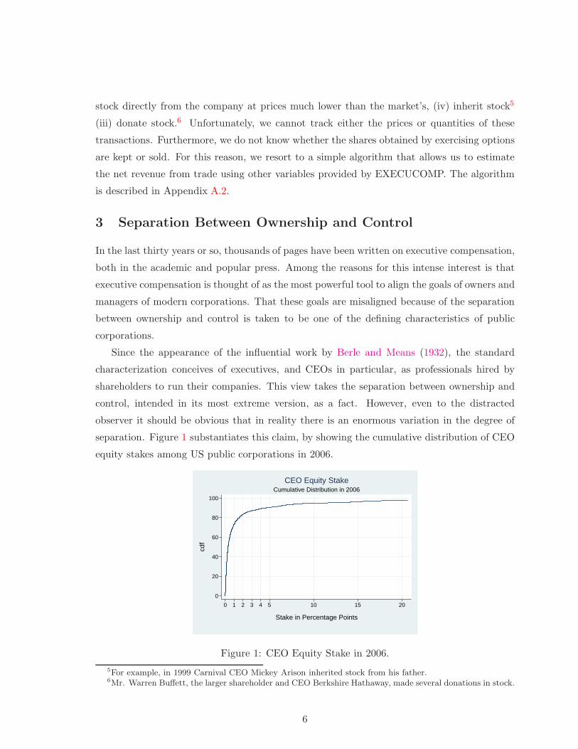
Since the appearance of the influential work by Berle and Means (1932), the standard

characterization conceives of executives, and CEOs in particular, as professionals hired by

shareholders to run their companies. This view takes the separation between ownership and

control, intended in its most extreme version, as a fact. However, even to the distracted

observer it should be obvious that in reality there is an enormous variation in the degree of

separation. Figure 1 substantiates this claim, by showing the cumulative distribution of CEO

equity stakes among US public corporations in 2006.

0

20

40

60

80

100

cdf

0 1 2 3 4 5 10 15 20

Stake in Percentage Points

Cumulative Distribution in 2006CEO Equity Stake

Figure 1: CEO Equity Stake in 2006.

5For example, in 1999 Carnival CEO Mickey Arison inherited stock from his father.6Mr. Warren Bu!ett, the larger shareholder and CEO Berkshire Hathaway, made several donations in stock.

6

Our data shows that in 2006, about 25% of CEOs held more than 1% of their companies’

common stock, and about 10% held more than 5%.7 CEOs with relatively low stock holding

fit the Berle and Means’ stereotype, in the sense that they are likely to have been hired only

to manage the company. This is the case, for example, of Mr. John W. Thompson, who

spent most of his career at IBM before being hired as Symantec’s CEO in 1999. In 2006, Mr.

Thompson held about 0.16% of the company’s common stock. The CEOs with the largest

equity stakes are far from the Berle and Means’ ideal and are likely to be either the companies’

founders or to have family ties to them. This is the case of Micky Arison, CEO of Carnival

Corporation – the world’s largest cruise operator – and son of Ted Arison, the company’s

founder. In 2006, Mr. Arison held about 23.8% of Carnival’s common stock.

As will be clear below, stocks have a primary role in incentive provision. In the case

of professional CEOs such as Symantec’s Mr. Thompson, the observed equity stake is the

result of the company’s compensation policy. Therefore, the incentives that result can be

used to assess the disciplining role of boards of directors. This is decidedly not the case for

company founders and for other executives, such as Mr. Arison, whose large equity holdings

have nothing to do with the company’s compensation policy. These individuals, although

disciplined by the requirements of public companies, essentially have absolute control over the

source of their pecuniary incentives. Compensation committees can have very little impact

on them.

In light of this simple argument, in the remainder of this paper we will report certain

statistics for Professional CEOs only, arbitrarily defined as those that hold less than 1% of

their companies’ common stock. Our goal is discern the di!erences, if any, in the way in which

professional CEOs are compensated and in the incentives they face.

4 The Distribution of Compensation across Executives

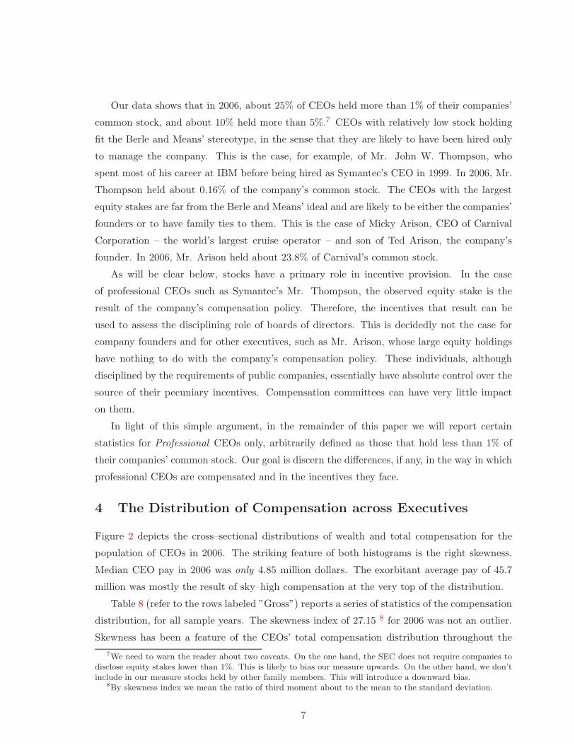
Figure 2 depicts the cross–sectional distributions of wealth and total compensation for the

population of CEOs in 2006. The striking feature of both histograms is the right skewness.

Median CEO pay in 2006 was only 4.85 million dollars. The exorbitant average pay of 45.7

million was mostly the result of sky–high compensation at the very top of the distribution.

Table 8 (refer to the rows labeled ”Gross”) reports a series of statistics of the compensation

distribution, for all sample years. The skewness index of 27.15 8 for 2006 was not an outlier.

Skewness has been a feature of the CEOs’ total compensation distribution throughout the

7We need to warn the reader about two caveats. On the one hand, the SEC does not require companies todisclose equity stakes lower than 1%. This is likely to bias our measure upwards. On the other hand, we don’tinclude in our measure stocks held by other family members. This will introduce a downward bias.

8By skewness index we mean the ratio of third moment about to the mean to the standard deviation.

7

sample period. Notice, however, that the distribution is not always right–skewed. In the three

(fiscal) years following the stock market peak of January 2000, the mean CEO compensation

was largely negative, while the median values were positive. The reason is that, as illustrated

in Section 5, CEOs of large companies have relatively high stock and option holdings. In turn,

this implies that their compensation is particularly sensitive to stock market fluctuations, of

either sign.

0

100

200

300

400

500

600

700

Med

ians

1 2 3 4 5 6 7 8 9 10 11 12 13 14 15 16 17 18 19 20Quantiles of Compensation Distribution

Millions of 2005 dollarsCEO wealth in 2006

−50

0

50

100

150

Med

ians

1 2 3 4 5 6 7 8 9 10 11 12 13 14 15 16 17 18 19 20Quantiles of Compensation Distribution

Millions of 2005 dollarsTotal CEO Yearly Compensation in 2006

Figure 2: CEO Compensation in 2006.

This leads us to another salient feature of the data. Contrary to what has become common

wisdom, CEOs do lose money. Sometimes, they lose a lot. In 2006, with the S&P 500 index

rising by more than 9%, our measure of compensation was negative for as many as 264 CEOs.

As expected, the big losers were those at the helm of companies whose stock dropped the most

in value during the year. Among them, Yahoo (–33%), Amazon (–20%), and Ebay(–30%).

Conversely, the winners were the chief executives of the companies whose shareholders gained

the most, such as Mc–Graw Hill (+30%), Marriott (+38%), and Comcast (+65%). Table

8 shows that a sizeable fraction of CEOs lost money in every year. In 2002, that fraction

exceeded 40%.

If executives hedge systematic risk, actual median gains and losses will be much smaller

(in absolute value) than our figures suggest. For this reason, we also report statistics for

Total Yearly Compensation, net of the return executives would have earned by investing their

wealth in the market portfolio. See the rows labeled “Net of Market” in Table 8.

The Net definition yields the actual compensation under the assumption that executives

hedge systematic risk by selling short the market portfolio or by building a similar position

by trading on derivatives.9

9An example of such a position is a zero–cost collar, which involves selling an out–of–the–money call option

8

Hedging systematic risk has a large e!ect on the tails of the compensation distribution. It

moderates losses in bad years for the stock market and moderates gains in good years. As a

result, median net compensation tends to be smaller than gross compensation in a good year

for the stock market, and larger in bad years. Table 8 shows that median net compensation

ranged between –$100,000 (in 1998) and $5.82 million (in 2003). The main message we draw

from these data, however, is the same as above. In every single year both dispersion and

skewness were remarkably large.

Since the SEC does not require executives to disclose trades in securities not issued by their

companies, we do not know whether executives indeed hedge market risk or not. However,

Garvey and Milbourn (2003) provides indirect evidence that this may be the case. They argue

that if companies recognize that they should use relative performance evaluation (RPE) only

for those executives that are unable to diversify systematic risk, estimates of pay–performance

sensitivity should depend on market volatility only in the case of younger and poorer execu-

tives, whose chances of diversification are slimmer. This is exactly what they found in their

study.

Refer once more to Table 8. The third row illustrates the results that obtain with the

classical definition of compensation. The picture it conveys is rather di!erent. In 2006,

mean and median CEO pay were $6.74 and $3.24 million , respectively. Interestingly, the

dispersion across executives is much lower than it is with our measure. According to the

classical definition, the mean compensation of the top 10% in the distribution was about

35 million dollars in 2006 (against our estimate of $450.33 million). The mean compensation

among the bottom 10% in 2002 was about $450,000, against a $336.86 million loss that obtains

according to our definition!

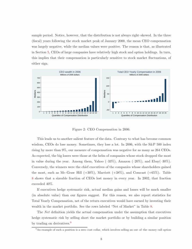
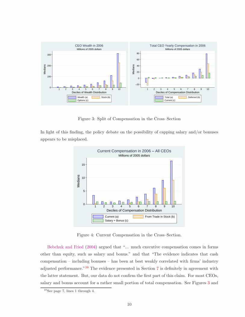
Table 9 provides detailed information about the partition of total yearly compensation

between Current and Deferred. A clear fact, better illustrated in Figure 3 in the case of 2006,

is the cross–sectional dispersion in the deferred component. Both big winners and big losers

have large stock and option portfolios. To appreciate this, consider that the median equity

stake among CEOs in the top and bottom deciles of the compensation distribution are 1.15

and 0.77%, respectively, against a 0.24% median for the remainder.

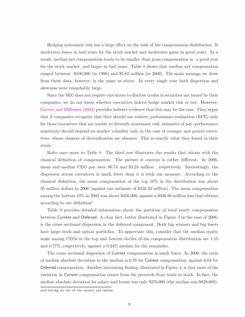
The cross–sectional dispersion of Current compensation is much lower. In 2006, the ratio

of median absolute deviation to the median is 0.76 for Current compensation, against 6.04 for

Deferred compensation. Another interesting finding, illustrated in Figure 4, is that most of the

variation in Current compensation comes from the proceeds from trade in stock. In fact, the

median absolute deviation for salary and bonus was only $270,000 (the median was $829,000).

and buying an out–of–the–money put option.

9

0

100

200

300

Med

ians

1 2 3 4 5 6 7 8 9 10Deciles of Wealth Distribution

Millions of 2005 dollarsCEO Wealth in 2006

Wealth (a) Stock (b)Options (c)

−20

0

20

40

60

80

Med

ians

1 2 3 4 5 6 7 8 9 10Deciles of Compensation Distribution

Millions of 2005 dollarsTotal CEO Yearly Compensation in 2006

Total (a) Deferred (b)Current (c)

Figure 3: Split of Compensation in the Cross–Section

In light of this finding, the policy debate on the possibility of capping salary and/or bonuses

appears to be misplaced.

0

5

10

15

Med

ians

1 2 3 4 5 6 7 8 9 10Deciles of Compensation Distribution

Millions of 2005 dollarsCurrent Compensation in 2006 − All CEOs

Current (a) From Trade in Stock (b)Salary + Bonus (c)

Figure 4: Current Compensation in the Cross–Section.

Bebchuk and Fried (2004) argued that “... much executive compensation comes in forms

other than equity, such as salary and bonus.” and that “The evidence indicates that cash

compensation – including bonuses – has been at best weakly correlated with firms’ industry

adjusted performance.”10 The evidence presented in Section 7 is definitely in agreement with

the latter statement. But, our data do not confirm the first part of this claim. For most CEOs,

salary and bonus account for a rather small portion of total compensation. See Figures 3 and

10See page 7, lines 1 through 4.

10

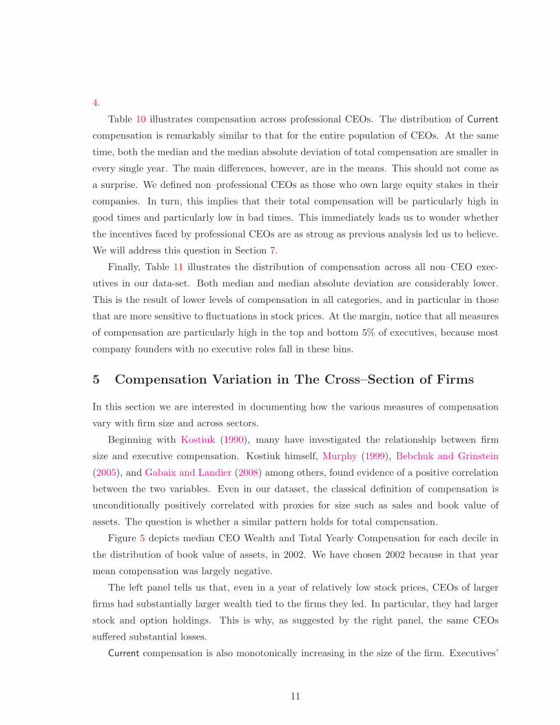
4.

Table 10 illustrates compensation across professional CEOs. The distribution of Current

compensation is remarkably similar to that for the entire population of CEOs. At the same

time, both the median and the median absolute deviation of total compensation are smaller in

every single year. The main di!erences, however, are in the means. This should not come as

a surprise. We defined non–professional CEOs as those who own large equity stakes in their

companies. In turn, this implies that their total compensation will be particularly high in

good times and particularly low in bad times. This immediately leads us to wonder whether

the incentives faced by professional CEOs are as strong as previous analysis led us to believe.

We will address this question in Section 7.

Finally, Table 11 illustrates the distribution of compensation across all non–CEO exec-

utives in our data-set. Both median and median absolute deviation are considerably lower.

This is the result of lower levels of compensation in all categories, and in particular in those

that are more sensitive to fluctuations in stock prices. At the margin, notice that all measures

of compensation are particularly high in the top and bottom 5% of executives, because most

company founders with no executive roles fall in these bins.

5 Compensation Variation in The Cross–Section of Firms

In this section we are interested in documenting how the various measures of compensation

vary with firm size and across sectors.

Beginning with Kostiuk (1990), many have investigated the relationship between firm

size and executive compensation. Kostiuk himself, Murphy (1999), Bebchuk and Grinstein

(2005), and Gabaix and Landier (2008) among others, found evidence of a positive correlation

between the two variables. Even in our dataset, the classical definition of compensation is

unconditionally positively correlated with proxies for size such as sales and book value of

assets. The question is whether a similar pattern holds for total compensation.

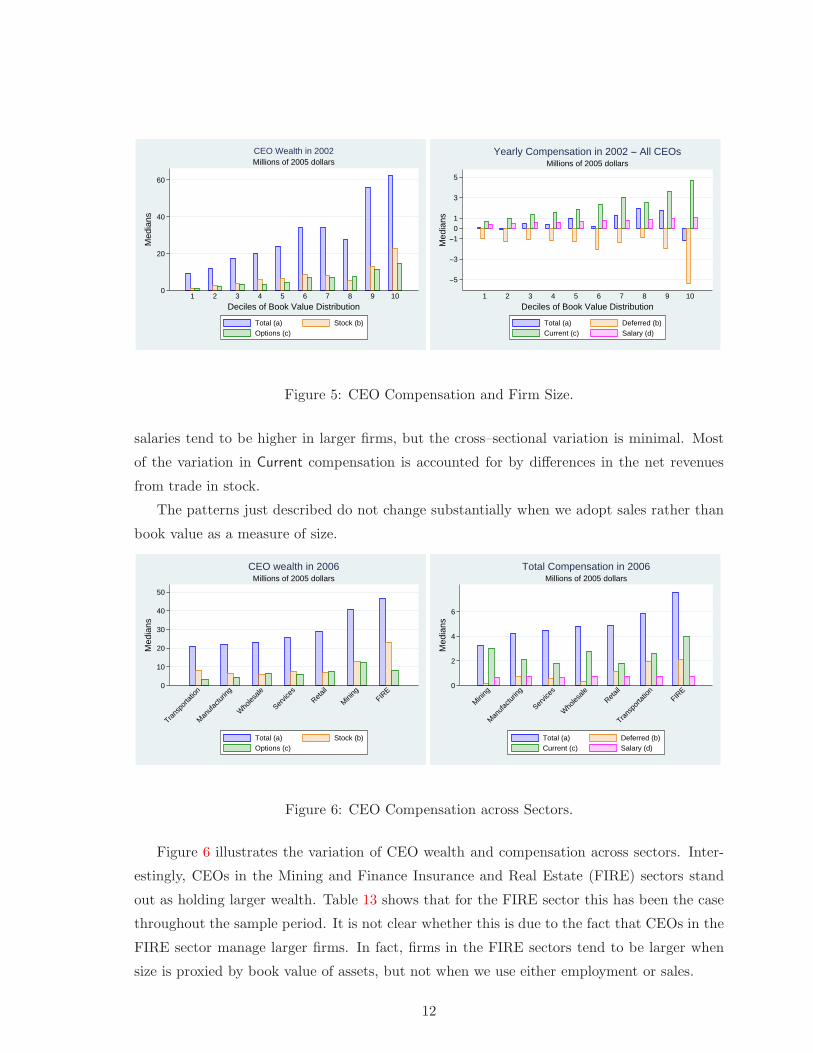
Figure 5 depicts median CEO Wealth and Total Yearly Compensation for each decile in

the distribution of book value of assets, in 2002. We have chosen 2002 because in that year

mean compensation was largely negative.

The left panel tells us that, even in a year of relatively low stock prices, CEOs of larger

firms had substantially larger wealth tied to the firms they led. In particular, they had larger

stock and option holdings. This is why, as suggested by the right panel, the same CEOs

su!ered substantial losses.

Current compensation is also monotonically increasing in the size of the firm. Executives’

11

0

20

40

60

Med

ians

1 2 3 4 5 6 7 8 9 10Deciles of Book Value Distribution

Millions of 2005 dollarsCEO Wealth in 2002

Total (a) Stock (b)Options (c)

−5

−3

−101

3

5

Med

ians

1 2 3 4 5 6 7 8 9 10Deciles of Book Value Distribution

Millions of 2005 dollarsYearly Compensation in 2002 − All CEOs

Total (a) Deferred (b)Current (c) Salary (d)

Figure 5: CEO Compensation and Firm Size.

salaries tend to be higher in larger firms, but the cross–sectional variation is minimal. Most

of the variation in Current compensation is accounted for by di!erences in the net revenues

from trade in stock.

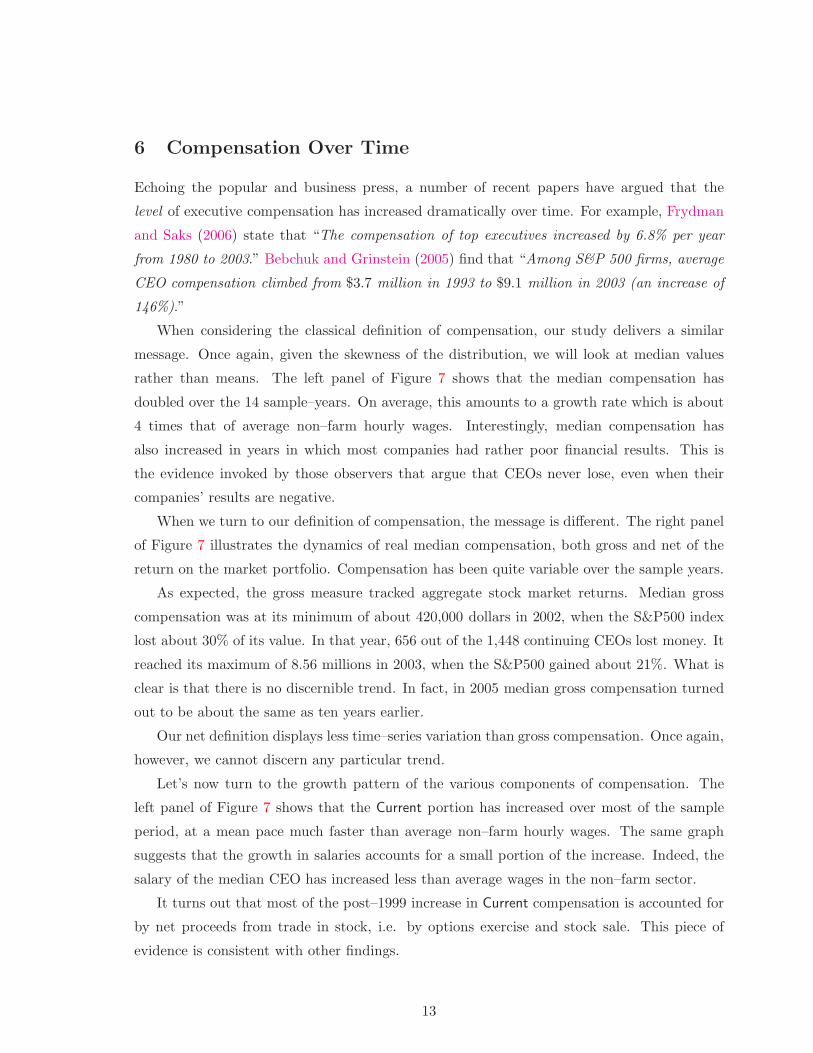
The patterns just described do not change substantially when we adopt sales rather than

book value as a measure of size.

0

10

20

30

40

50

Med

ians

Transp

ortati

on

Manufa

cturin

g

Wholes

ale

Service

sReta

il

Mining

FIRE

Millions of 2005 dollarsCEO wealth in 2006

Total (a) Stock (b)Options (c)

0

2

4

6

Med

ians

Mining

Manufa

cturin

g

Service

s

Wholes

aleReta

il

Transp

ortati

onFIRE

Millions of 2005 dollarsTotal Compensation in 2006

Total (a) Deferred (b)Current (c) Salary (d)

Figure 6: CEO Compensation across Sectors.

Figure 6 illustrates the variation of CEO wealth and compensation across sectors. Inter-

estingly, CEOs in the Mining and Finance Insurance and Real Estate (FIRE) sectors stand

out as holding larger wealth. Table 13 shows that for the FIRE sector this has been the case

throughout the sample period. It is not clear whether this is due to the fact that CEOs in the

FIRE sector manage larger firms. In fact, firms in the FIRE sectors tend to be larger when

size is proxied by book value of assets, but not when we use either employment or sales.

12

6 Compensation Over Time

Echoing the popular and business press, a number of recent papers have argued that the

level of executive compensation has increased dramatically over time. For example, Frydman

and Saks (2006) state that “The compensation of top executives increased by 6.8% per year

from 1980 to 2003.” Bebchuk and Grinstein (2005) find that “Among S&P 500 firms, average

CEO compensation climbed from $3.7 million in 1993 to $9.1 million in 2003 (an increase of

146%).”

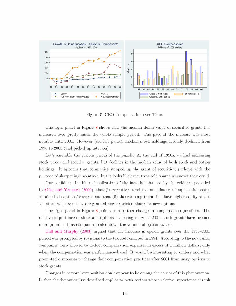
When considering the classical definition of compensation, our study delivers a similar

message. Once again, given the skewness of the distribution, we will look at median values

rather than means. The left panel of Figure 7 shows that the median compensation has

doubled over the 14 sample–years. On average, this amounts to a growth rate which is about

4 times that of average non–farm hourly wages. Interestingly, median compensation has

also increased in years in which most companies had rather poor financial results. This is

the evidence invoked by those observers that argue that CEOs never lose, even when their

companies’ results are negative.

When we turn to our definition of compensation, the message is di!erent. The right panel

of Figure 7 illustrates the dynamics of real median compensation, both gross and net of the

return on the market portfolio. Compensation has been quite variable over the sample years.

As expected, the gross measure tracked aggregate stock market returns. Median gross

compensation was at its minimum of about 420,000 dollars in 2002, when the S&P500 index

lost about 30% of its value. In that year, 656 out of the 1,448 continuing CEOs lost money. It

reached its maximum of 8.56 millions in 2003, when the S&P500 gained about 21%. What is

clear is that there is no discernible trend. In fact, in 2005 median gross compensation turned

out to be about the same as ten years earlier.

Our net definition displays less time–series variation than gross compensation. Once again,

however, we cannot discern any particular trend.

Let’s now turn to the growth pattern of the various components of compensation. The

left panel of Figure 7 shows that the Current portion has increased over most of the sample

period, at a mean pace much faster than average non–farm hourly wages. The same graph

suggests that the growth in salaries accounts for a small portion of the increase. Indeed, the

salary of the median CEO has increased less than average wages in the non–farm sector.

It turns out that most of the post–1999 increase in Current compensation is accounted for

by net proceeds from trade in stock, i.e. by options exercise and stock sale. This piece of

evidence is consistent with other findings.

13

100

120

140

160

180

200

93 94 95 96 97 98 99 00 01 02 03 04 05 06

Salary CurrentAvg Non−Farm Hourly Wages Classical Definition

Medians − 1993=100Growth in Compensation − Selected Components

0

2

4

6

8

Med

ians

93 94 95 96 97 98 99 00 01 02 03 04 05 06

Millions of 2005 dollarsCEO Compensation

Gross Definition (a) Net Definition (b)Classical Definition (c)

Figure 7: CEO Compensation over Time.

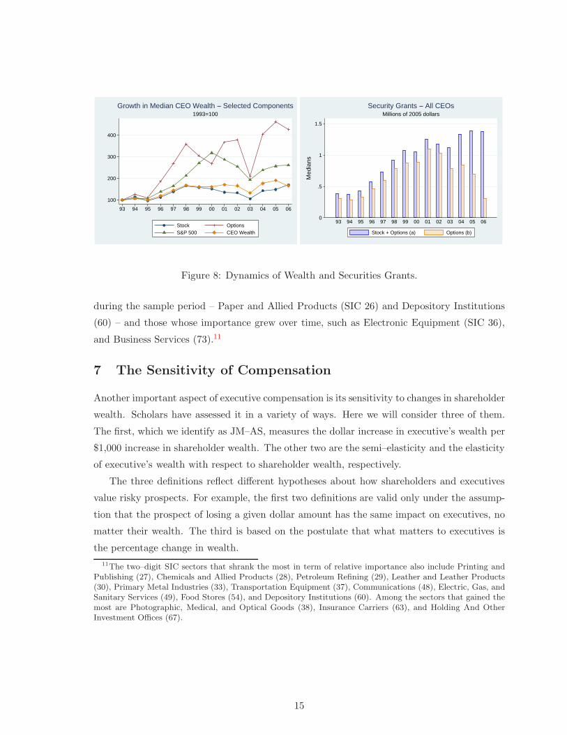
The right panel in Figure 8 shows that the median dollar value of securities grants has

increased over pretty much the whole sample period. The pace of the increase was most

notable until 2001. However (see left panel), median stock holdings actually declined from

1998 to 2003 (and picked up later on).

Let’s assemble the various pieces of the puzzle. At the end of 1990s, we had increasing

stock prices and security grants, but declines in the median value of both stock and option

holdings. It appears that companies stepped up the grant of securities, perhaps with the

purpose of sharpening incentives, but it looks like executives sold shares whenever they could.

Our confidence in this rationalization of the facts is enhanced by the evidence provided

by Ofek and Yermack (2000), that (i) executives tend to immediately relinquish the shares

obtained via options’ exercise and that (ii) those among them that have higher equity stakes

sell stock whenever they are granted new restricted shares or new options.

The right panel in Figure 8 points to a further change in compensation practices. The

relative importance of stock and options has changed. Since 2001, stock grants have become

more prominent, as companies scaled down the volume of option awards.

Hall and Murphy (2003) argued that the increase in option grants over the 1995–2001

period was prompted by revisions to the tax code enacted in 1994. According to the new rules,

companies were allowed to deduct compensation expenses in excess of 1 million dollars, only

when the compensation was performance–based. It would be interesting to understand what

prompted companies to change their compensation practices after 2001 from using options to

stock grants.

Changes in sectoral composition don’t appear to be among the causes of this phenomenon.

In fact the dynamics just described applies to both sectors whose relative importance shrank

14

100

200

300

400

93 94 95 96 97 98 99 00 01 02 03 04 05 06

Stock OptionsS&P 500 CEO Wealth

1993=100Growth in Median CEO Wealth − Selected Components

0

.5

1

1.5

Med

ians

93 94 95 96 97 98 99 00 01 02 03 04 05 06

Millions of 2005 dollarsSecurity Grants − All CEOs

Stock + Options (a) Options (b)

Figure 8: Dynamics of Wealth and Securities Grants.

during the sample period – Paper and Allied Products (SIC 26) and Depository Institutions

(60) – and those whose importance grew over time, such as Electronic Equipment (SIC 36),

and Business Services (73).11

7 The Sensitivity of Compensation

Another important aspect of executive compensation is its sensitivity to changes in shareholder

wealth. Scholars have assessed it in a variety of ways. Here we will consider three of them.

The first, which we identify as JM–AS, measures the dollar increase in executive’s wealth per

$1,000 increase in shareholder wealth. The other two are the semi–elasticity and the elasticity

of executive’s wealth with respect to shareholder wealth, respectively.

The three definitions reflect di!erent hypotheses about how shareholders and executives

value risky prospects. For example, the first two definitions are valid only under the assump-

tion that the prospect of losing a given dollar amount has the same impact on executives, no

matter their wealth. The third is based on the postulate that what matters to executives is

the percentage change in wealth.

11The two–digit SIC sectors that shrank the most in term of relative importance also include Printing andPublishing (27), Chemicals and Allied Products (28), Petroleum Refining (29), Leather and Leather Products(30), Primary Metal Industries (33), Transportation Equipment (37), Communications (48), Electric, Gas, andSanitary Services (49), Food Stores (54), and Depository Institutions (60). Among the sectors that gained themost are Photographic, Medical, and Optical Goods (38), Insurance Carriers (63), and Holding And OtherInvestment O"ces (67).

15

7.1 The JM–AS Sensitivity Measure

The acronym JM–AS refers to the contributions by Jensen and Murphy (1990) and Aggarwal

and Samwick (1999). Having found that in their sample CEO wealth increased by only $3.25

for 1,000 dollar increase in shareholder wealth, Jensen and Murphy (1990) claimed that CEOs

were paid like bureaucrats. Or, in other words, that they faced rather weak incentives.

Schaefer (1998) and Hall and Liebman (1998) showed that Jensen and Murphy (1990)’s

estimate was low because their sample was biased towards large firms. Stock market capital-

ization fluctuates more for large firms than it does for small firms. This implies that the risk

imposed on a CEO by a given pay–performance sensitivity tends to be larger, the larger the

firm.

This motivates us to follow the lead of Aggarwal and Samwick (1999), and compute esti-

mates of sensitivity at di!erent levels of volatility.

−150

−100

−50

0

50

100

150

Tota

l Com

pens

atio

n (M

illion

s)

−15 −10 −5 0 5 10 15

Net Shareholder Gain (Billions)

2005 dollarsTotal Yearly Compensation and Shareholder Gain

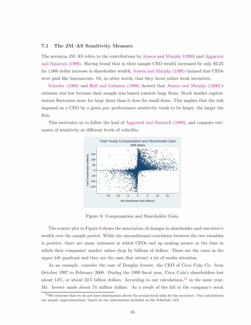
Figure 9: Compensation and Shareholder Gain.

The scatter plot in Figure 9 shows the association of changes in shareholder and executive’s

wealth over the sample period. While the unconditional correlation between the two variables

is positive, there are many instances in which CEOs end up making money at the time in

which their companies’ market values drop by billions of dollars. These are the cases in the

upper left quadrant and they are the ones that attract a lot of media attention.

As an example, consider the case of Douglas Ivester, the CEO of Coca–Cola Co. from

October 1997 to February 2000. During the 1999 fiscal year, Coca–Cola’s shareholders lost

about 14%, or about 22.5 billion dollars. According to our calculations,12 in the same year,

Mr. Ivester made about 74 million dollars. As a result of the fall in the company’s stock

12We reiterate that we do not have information about the actual stock sales by the executive. Our calculationsare simply approximations, based on the information included in the Schedule 14A.

16

price, the value of his stock holding dropped. This explains why his Deferred compensation

was negative (about –60.65 millions). However, his Current compensation was roughly $135

million, 91 of which came from the sale of company’s stock.13

Following Aggarwal and Samwick (1999), we estimate the following equation:

wijt = !0 + !1"MKT CAPjt + !2"MKT CAPjt " F ("j) + !3F ("j) + #t + $it, (1)

where i, j, t index the executive, the firm, and time, respectively. The letter w denotes com-

pensation, MKT CAPjt is total market capitalization, " is the one–period lag operator, and

#t is a year dummy whose purpose is to control for aggregate shocks. Finally, "jt denotes

the standard deviation in shareholders’ dollar return (i.e. the change in market capital-

ization). F (·) is the cumulative distribution of standard deviations. The interaction term

"MKT CAPjt " F ("j) was introduced because the impact on compensation of a 1, 000 dol-

lar change in shareholder wealth is expected to be larger, the smaller the average change in

capitalization. The measure of sensitivity for company j in year t will be !1 + !2 " F ("jt).

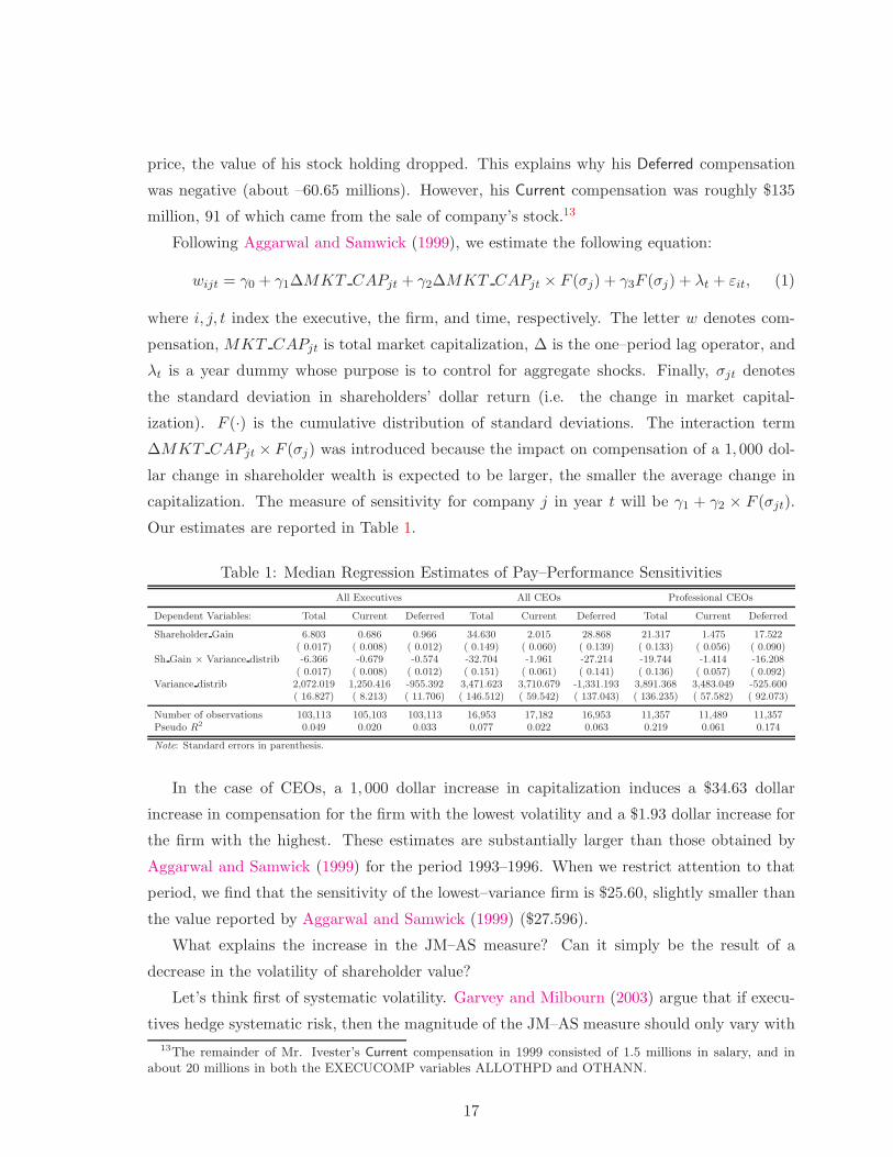
Our estimates are reported in Table 1.

Table 1: Median Regression Estimates of Pay–Performance Sensitivities

All Executives All CEOs Professional CEOs

Dependent Variables: Total Current Deferred Total Current Deferred Total Current Deferred

Shareholder Gain 6.803 0.686 0.966 34.630 2.015 28.868 21.317 1.475 17.522( 0.017) ( 0.008) ( 0.012) ( 0.149) ( 0.060) ( 0.139) ( 0.133) ( 0.056) ( 0.090)

Sh Gain ! Variance distrib -6.366 -0.679 -0.574 -32.704 -1.961 -27.214 -19.744 -1.414 -16.208( 0.017) ( 0.008) ( 0.012) ( 0.151) ( 0.061) ( 0.141) ( 0.136) ( 0.057) ( 0.092)

Variance distrib 2,072.019 1,250.416 -955.392 3,471.623 3,710.679 -1,331.193 3,891.368 3,483.049 -525.600( 16.827) ( 8.213) ( 11.706) ( 146.512) ( 59.542) ( 137.043) ( 136.235) ( 57.582) ( 92.073)

Number of observations 103,113 105,103 103,113 16,953 17,182 16,953 11,357 11,489 11,357Pseudo R

2 0.049 0.020 0.033 0.077 0.022 0.063 0.219 0.061 0.174

Note: Standard errors in parenthesis.

In the case of CEOs, a 1, 000 dollar increase in capitalization induces a $34.63 dollar

increase in compensation for the firm with the lowest volatility and a $1.93 dollar increase for

the firm with the highest. These estimates are substantially larger than those obtained by

Aggarwal and Samwick (1999) for the period 1993–1996. When we restrict attention to that

period, we find that the sensitivity of the lowest–variance firm is $25.60, slightly smaller than

the value reported by Aggarwal and Samwick (1999) ($27.596).

What explains the increase in the JM–AS measure? Can it simply be the result of a

decrease in the volatility of shareholder value?

Let’s think first of systematic volatility. Garvey and Milbourn (2003) argue that if execu-

tives hedge systematic risk, then the magnitude of the JM–AS measure should only vary with

13The remainder of Mr. Ivester’s Current compensation in 1999 consisted of 1.5 millions in salary, and inabout 20 millions in both the EXECUCOMP variables ALLOTHPD and OTHANN.

17

the idiosyncratic portion of the volatility of shareholder’s wealth. They provide evidence that

this is indeed the case between 1992 and 1998. We followed their methodology and retrieved

measures of systematic and idiosyncratic volatility by means of simple CAPM regressions.

Then, we modified equation (1) by replacing the c.d.f. of firm volatility with the distributions

of systematic and idiosyncratic volatility.

Our results are reported in Table 14. The bottom line is that the relationship between

the sensitivity measure and volatility is accounted for almost completely by the idiosyncratic

portion of the latter. This also means that changes in systematic volatility are not likely to

rationalize the increase in the sensitivity measure we have documented.

How about changes in idiosyncratic risk? Brandt, Brav, and Kumar (2009) found that

the idiosyncratic volatility of percent returns declined over the 1997–2007 period. Obviously,

this may matter. There are at least two reasons, however, why this may not be the whole

story. First of all, the volatility of shareholder wealth also depends on market valuation, which

has increased over the period in exam. Furthermore, Brandt, Brav, and Kumar (2009) argue

that most of the decline in volatility applied to a subset of stocks (low price stocks, held

proportionally more by retail investors). This means that the decline in volatility may have a

sizeable impact on OLS estimates, but should have a more limited e!ect on median estimates.

The results reported so far suggest that the increase in performance–based compensation

may have led to stronger incentives. The next two sections will tell us whether our other

measures of pay–performance sensitivity yield a consistent picture.

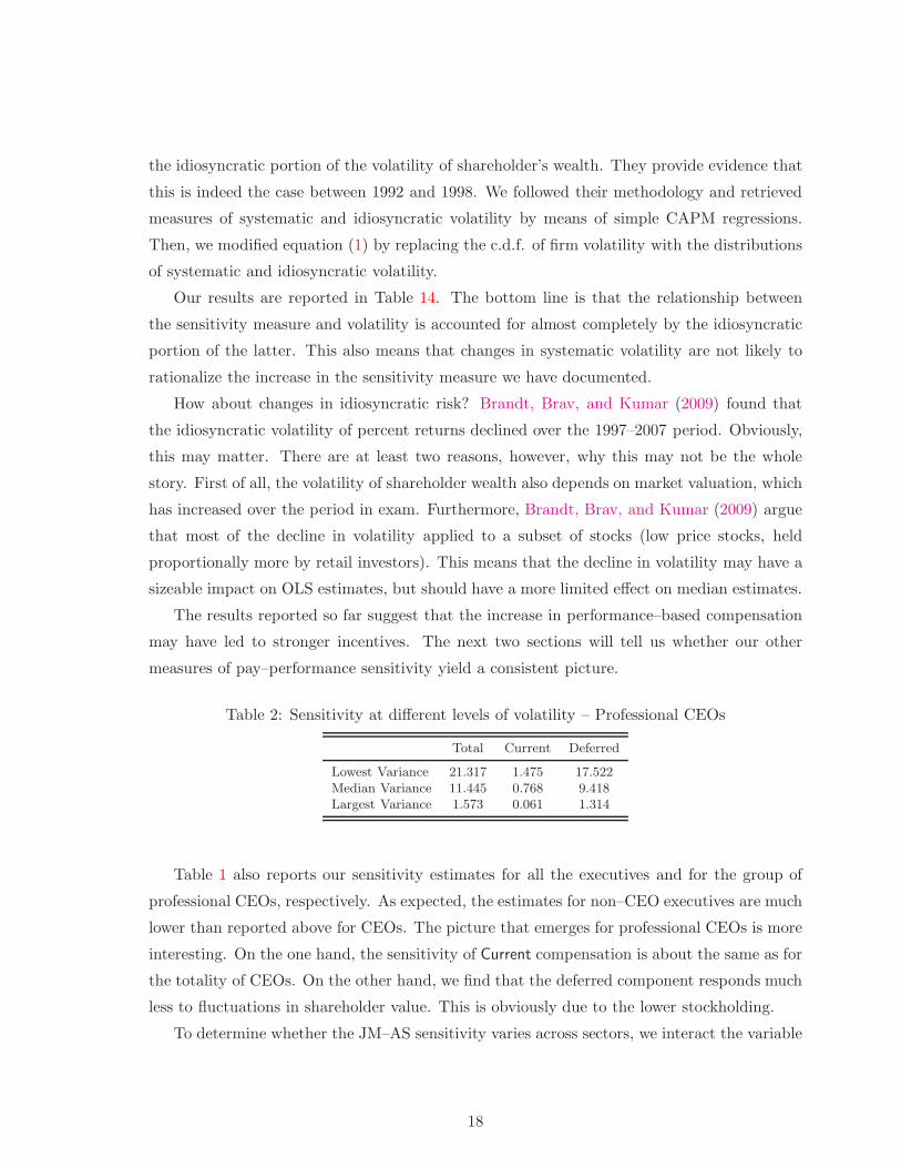
Table 2: Sensitivity at di!erent levels of volatility – Professional CEOs

Total Current Deferred

Lowest Variance 21.317 1.475 17.522Median Variance 11.445 0.768 9.418Largest Variance 1.573 0.061 1.314

Table 1 also reports our sensitivity estimates for all the executives and for the group of

professional CEOs, respectively. As expected, the estimates for non–CEO executives are much

lower than reported above for CEOs. The picture that emerges for professional CEOs is more

interesting. On the one hand, the sensitivity of Current compensation is about the same as for

the totality of CEOs. On the other hand, we find that the deferred component responds much

less to fluctuations in shareholder value. This is obviously due to the lower stockholding.

To determine whether the JM–AS sensitivity varies across sectors, we interact the variable

18

"MKT CAPjt with sector–specific dummies. We estimate the equation

wijt = !0 + !1"MKT CAPjt " %s + !2"MKT CAPjt " F ("j) + !3F ("j) + $it,

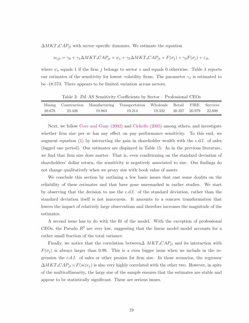
where %s equals 1 if the firm j belongs to sector s and equals 0 otherwise. Table 3 reports

our estimates of the sensitivity for lowest–volatility firms. The parameter !1 is estimated to

be -18.573. There appears to be limited variation across sectors.

Table 3: JM–AS Sensitivity Coe#cients by Sector – Professional CEOs

Mining Construction Manufacturing Transportation Wholesale Retail FIRE Services

20.678 23.426 19.863 19.214 19.332 20.327 20.979 22.698

Next, we follow Core and Guay (2002) and Cichello (2005) among others, and investigate

whether firm size per–se has any e!ect on pay–performance sensitivity. To this end, we

augment equation (1) by interacting the gain in shareholder wealth with the c.d.f. of sales

(lagged one period). Our estimates are displayed in Table 15. As in the previous literature,

we find that firm size does matter. That is, even conditioning on the standard deviation of

shareholders’ dollar return, the sensitivity is negatively associated to size. Our findings do

not change qualitatively when we proxy size with book value of assets.

We conclude this section by outlining a few basic issues that cast some doubts on the

reliability of these estimates and that have gone unremarked in earlier studies. We start

by observing that the decision to use the c.d.f. of the standard deviation, rather than the

standard deviation itself is not innocuous. It amounts to a concave transformation that

lowers the impact of relatively large observations and therefore increases the magnitude of the

estimates.

A second issue has to do with the fit of the model. With the exception of professional

CEOs, the Pseudo R2 are very low, suggesting that the linear model model accounts for a

rather small fraction of the total variance.

Finally, we notice that the correlation between" MKT CAPjt and its interaction with

F ("j) is always larger than 0.99. This is a even bigger issue when we include in the re-

gression the c.d.f. of sales or other proxies for firm size. In those scenarios, the regressor

"MKT CAPjt"F (sizej) is also very highly correlated with the other two. However, in spite

of the multicollinearity, the large size of the sample ensures that the estimates are stable and

appear to be statistically significant. These are serious issues.

19

7.2 The Semi–Elasticity of Compensation with Respect to ShareholderWealth

The semi–elasticity measures the dollar increase in executive’s wealth associated with a 1%

increase in shareholder wealth. We estimate the following equation:

wijt = !0 + !1Sh %Gainjt + !2Sh %Gainjt " F ("j) + !3F ("j) + #t + $it, (2)

where Sh %Gainjt is the percentage gain of firm j’s shareholders over the fiscal year t. Here

"jt represents the standard deviation of shareholder percent return. F (·) is the c.d.f of the

standard deviation.

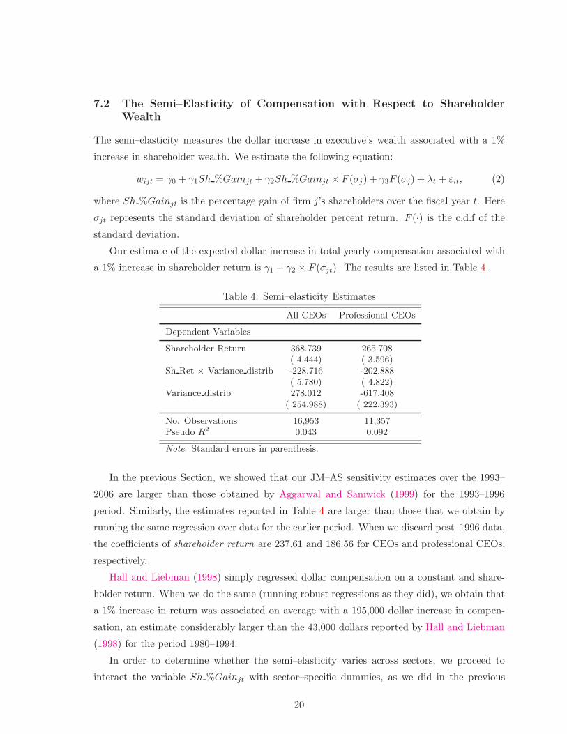
Our estimate of the expected dollar increase in total yearly compensation associated with

a 1% increase in shareholder return is !1 + !2 " F ("jt). The results are listed in Table 4.

Table 4: Semi–elasticity Estimates

All CEOs Professional CEOs

Dependent Variables

Shareholder Return 368.739 265.708( 4.444) ( 3.596)

Sh Ret ! Variance distrib -228.716 -202.888( 5.780) ( 4.822)

Variance distrib 278.012 -617.408( 254.988) ( 222.393)

No. Observations 16,953 11,357Pseudo R

2 0.043 0.092

Note: Standard errors in parenthesis.

In the previous Section, we showed that our JM–AS sensitivity estimates over the 1993–

2006 are larger than those obtained by Aggarwal and Samwick (1999) for the 1993–1996

period. Similarly, the estimates reported in Table 4 are larger than those that we obtain by

running the same regression over data for the earlier period. When we discard post–1996 data,

the coe#cients of shareholder return are 237.61 and 186.56 for CEOs and professional CEOs,

respectively.

Hall and Liebman (1998) simply regressed dollar compensation on a constant and share-

holder return. When we do the same (running robust regressions as they did), we obtain that

a 1% increase in return was associated on average with a 195,000 dollar increase in compen-

sation, an estimate considerably larger than the 43,000 dollars reported by Hall and Liebman

(1998) for the period 1980–1994.

In order to determine whether the semi–elasticity varies across sectors, we proceed to

interact the variable Sh %Gainjt with sector–specific dummies, as we did in the previous

20

section. The estimate of !2 is #183.137. Table 5 reports our estimates of the sensitivity for

lowest–volatility firms.

Table 5: Semi–elasticities by Sector – Professional CEOs

Mining Construction Manufacturing Transportation Wholesale Retail FIRE Services

215.850 230.859 252.287 201.615 191.395 268.963 365.961 291.699

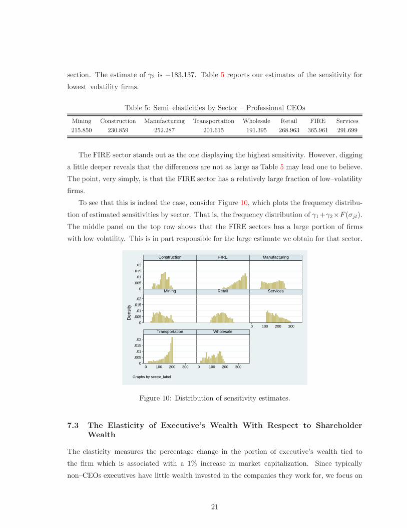
The FIRE sector stands out as the one displaying the highest sensitivity. However, digging

a little deeper reveals that the di!erences are not as large as Table 5 may lead one to believe.

The point, very simply, is that the FIRE sector has a relatively large fraction of low–volatility

firms.

To see that this is indeed the case, consider Figure 10, which plots the frequency distribu-

tion of estimated sensitivities by sector. That is, the frequency distribution of !1+!2"F ("jt).

The middle panel on the top row shows that the FIRE sectors has a large portion of firms

with low volatility. This is in part responsible for the large estimate we obtain for that sector.

0.005

.01.015

.02

0.005

.01.015

.02

0.005

.01.015

.02

0 100 200 300

0 100 200 300 0 100 200 300

Construction FIRE Manufacturing

Mining Retail Services

Transportation Wholesale

Dens

ity

Graphs by sector_label

Figure 10: Distribution of sensitivity estimates.

7.3 The Elasticity of Executive’s Wealth With Respect to ShareholderWealth

The elasticity measures the percentage change in the portion of executive’s wealth tied to

the firm which is associated with a 1% increase in market capitalization. Since typically

non–CEOs executives have little wealth invested in the companies they work for, we focus on

21

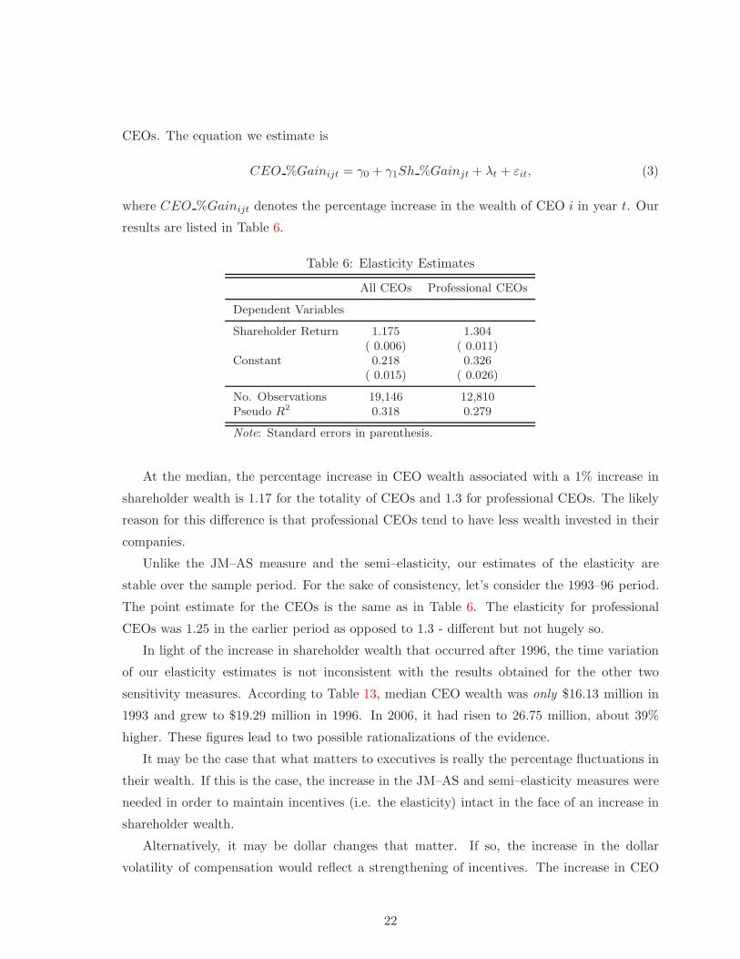
CEOs. The equation we estimate is

CEO %Gainijt = !0 + !1Sh %Gainjt + #t + $it, (3)

where CEO %Gainijt denotes the percentage increase in the wealth of CEO i in year t. Our

results are listed in Table 6.

Table 6: Elasticity Estimates

All CEOs Professional CEOs

Dependent Variables

Shareholder Return 1.175 1.304( 0.006) ( 0.011)

Constant 0.218 0.326( 0.015) ( 0.026)

No. Observations 19,146 12,810Pseudo R

2 0.318 0.279

Note: Standard errors in parenthesis.

At the median, the percentage increase in CEO wealth associated with a 1% increase in

shareholder wealth is 1.17 for the totality of CEOs and 1.3 for professional CEOs. The likely

reason for this di!erence is that professional CEOs tend to have less wealth invested in their

companies.

Unlike the JM–AS measure and the semi–elasticity, our estimates of the elasticity are

stable over the sample period. For the sake of consistency, let’s consider the 1993–96 period.

The point estimate for the CEOs is the same as in Table 6. The elasticity for professional

CEOs was 1.25 in the earlier period as opposed to 1.3 - di!erent but not hugely so.

In light of the increase in shareholder wealth that occurred after 1996, the time variation

of our elasticity estimates is not inconsistent with the results obtained for the other two

sensitivity measures. According to Table 13, median CEO wealth was only $16.13 million in

1993 and grew to $19.29 million in 1996. In 2006, it had risen to 26.75 million, about 39%

higher. These figures lead to two possible rationalizations of the evidence.

It may be the case that what matters to executives is really the percentage fluctuations in

their wealth. If this is the case, the increase in the JM–AS and semi–elasticity measures were

needed in order to maintain incentives (i.e. the elasticity) intact in the face of an increase in

shareholder wealth.

Alternatively, it may be dollar changes that matter. If so, the increase in the dollar

volatility of compensation would reflect a strengthening of incentives. The increase in CEO

22

wealth may have been necessary in order to retain CEOs in the faceof the higher risk they are

called to bear.

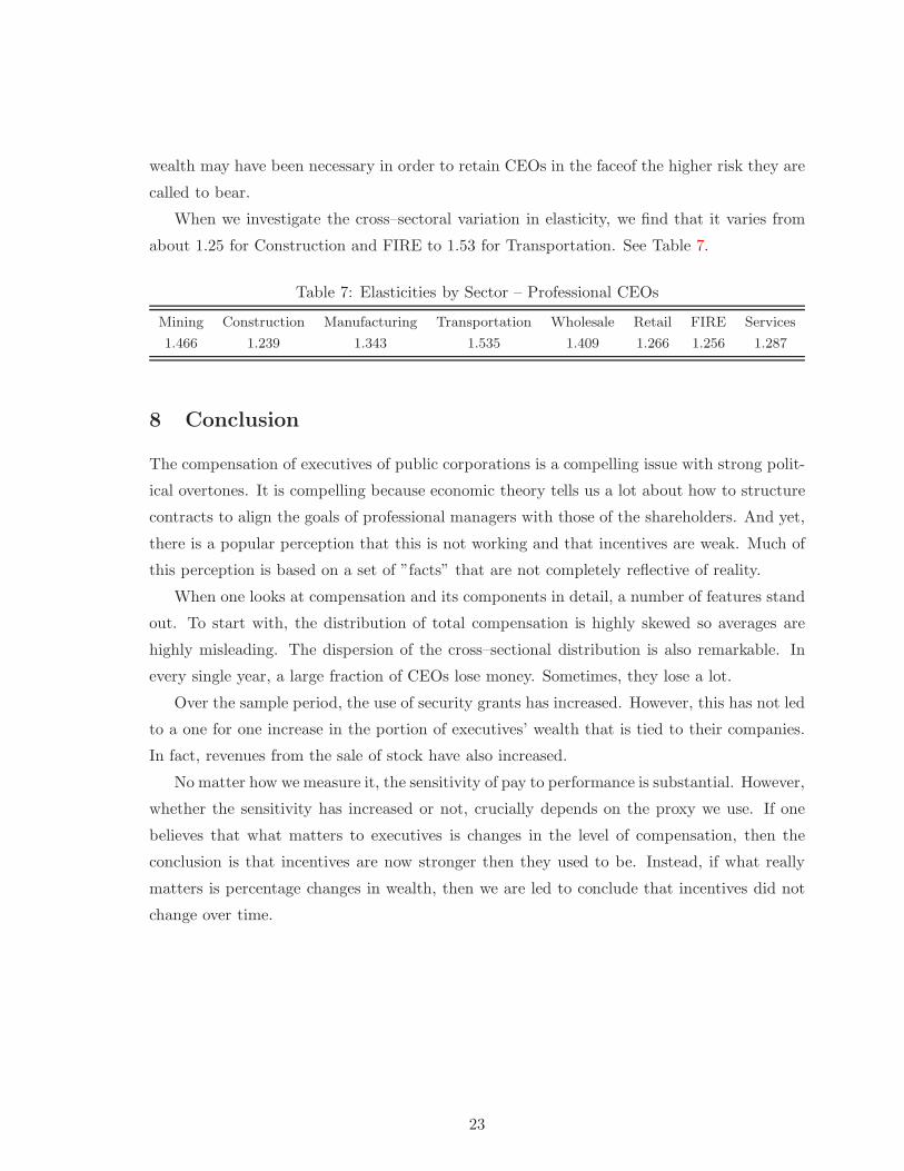
When we investigate the cross–sectoral variation in elasticity, we find that it varies from

about 1.25 for Construction and FIRE to 1.53 for Transportation. See Table 7.

Table 7: Elasticities by Sector – Professional CEOs

Mining Construction Manufacturing Transportation Wholesale Retail FIRE Services

1.466 1.239 1.343 1.535 1.409 1.266 1.256 1.287

8 Conclusion

The compensation of executives of public corporations is a compelling issue with strong polit-

ical overtones. It is compelling because economic theory tells us a lot about how to structure

contracts to align the goals of professional managers with those of the shareholders. And yet,

there is a popular perception that this is not working and that incentives are weak. Much of

this perception is based on a set of ”facts” that are not completely reflective of reality.

When one looks at compensation and its components in detail, a number of features stand

out. To start with, the distribution of total compensation is highly skewed so averages are

highly misleading. The dispersion of the cross–sectional distribution is also remarkable. In

every single year, a large fraction of CEOs lose money. Sometimes, they lose a lot.

Over the sample period, the use of security grants has increased. However, this has not led

to a one for one increase in the portion of executives’ wealth that is tied to their companies.

In fact, revenues from the sale of stock have also increased.

No matter how we measure it, the sensitivity of pay to performance is substantial. However,

whether the sensitivity has increased or not, crucially depends on the proxy we use. If one

believes that what matters to executives is changes in the level of compensation, then the

conclusion is that incentives are now stronger then they used to be. Instead, if what really

matters is percentage changes in wealth, then we are led to conclude that incentives did not

change over time.

23

A Definitions of CEO Wealth and Total Yearly Compensation

As stated in the main body of the paper, our definition of Executive’s Wealth proxyes for the

dollar value of the executive’s wealth that is tied to the firm at the beginning of the year. It

is defined as the sum of the following elements:

1. Market Value of Stock – SHROWN"PRCCF, where SHROWN is the number of shares

owned at the end of the previous fiscal year and PRCCF is the share price at the same

date

2. Market Value of Stock Options – INMONEX+INMONUN, where INMONEX is the

value of exercisable in–the–money options and INMONUN is the value of unexercisable

in–the–money options

3. Salary

4. Bonus

5. Total value of Restricted Stock Granted – RSTKGRNT

6. Total value of Stock Options Granted – SOPTVAL

7. Expected Discounted Value of Future Cash Payments – See Appendix A.3 below

Total Yearly Compensation is our best estimate of the net increase in executive’s wealth

that occurred during the fiscal year, due to her relation with the company. It is defined as

the sum of the following elements:

1. Salary

2. Bonus

3. Net revenue from Trade in Stock – See Appendix A.2 below

4. Dividends

5. Long–Term Incentive Payouts – ALLOTHTOT-ALLOTHPD

6. A miscellanea of items, among which payouts for cancellation of stock options, payment

for unused vacation, tax reimbursements, and signing bonuses – ALLOTHPD+OTHANN

7. Yearly change in the Market Value of Stock

24

8. Yearly change in the Market Value of Options

The first six elements define what we call Current Compensation. The sum of the remaining

ones identify Deferred Compensation.

A.1 The Value of Option Holdings according to the HH Algorithm

The analysis carried out in the main body of the paper posits that the change in the value of

the executive’s option holdings equals the year–on–year change in the sum of un-exercisable

and in–the–money options, both computed at the money at the end of the fiscal year. This is

strategy followed by most other studies, among which Aggarwal and Samwick (1999).

In this section we describe the algorithm devised by Himmelberg and Hubbard (2000)

in order to estimate the value of out–of–the–money options in executives’ portfolios. The

algorithm makes use of the following EXECUCOMP variables:14

• UEXNUMEX = number or un-exercised but exercisable options held by the executive

at year–end, both in–the–money and out–of–the–money

• UEXNUMUN = number of un-exercisable un-exercised options held by the executive at

year–end, both in–the–money and out–of–the–money

• SOPTEXSH = number of options exercised by the executive during the fiscal year

• SOPTGRN = total number of stock options awarded during the fiscal year

• SOPTVAL = total value of options granted during the fiscal year

Under the assumption that none of the options awarded in a given year are immediately

exercisable, the total value of options at year–end is the sum of (i) the value of newly granted

options (SOPTVAL), (ii) the value of un–exercisable options (in number UEXNUMUNt #

SOPTGRNt), and (iii) the value of exercisable options (in number UEXNUMEXt).

Unfortunately we lack data on strike prices and vesting horizons of the options in portfolio.

Therefore we assume that (i) a stock option grant vests gradually over four years, at a constant

rate and (ii) SOPTEXSH includes the options that are let expire. It follows that the laws of

14Some of the variables have changed labels in the latest version of the EXECUCOMP dataset.UEXNUMEX is now called OPT UNEX EXER NUM. UEXNUMUN is OPT UNEX UNEXER NUM. OP-TION EXER NUM. SOPTEXSH is OPTION EXER NUM. SOPTGRNT is OPTION AWARDS NUM. Fi-nally, OPTION AWARDS RPT VALUE coincides with SOPTVAL. However, the latest version of the datasetuses OPTION AWARDS FV for those records that follow the new FASB123 reporting requirements.

25

motion for the stocks of un–exercisable and exercisable options are

UEXNUMUNt = (1# 0.25)UEXNUMUNt!1 + SOPTGRNTt

UEXNUMEXt = 0.25 " UEXNUMUNt!1 + UEXNUMEXt!1 # SOPTEXSHt.

Then, we compute the value of the executive’s option portfolio to be

opvtt = SOPTV ALt+UEXNUMEXt " bsvext + [0.75"UEXNUMUNt!1]" bsvunt. (4)

The second addendum is the value of the exercisable options. The third addendum is the value

of un-exercisable options inherited from the past.15 We need to determine UEXNUMUNt!1.

Without it, we would have to discard one more observation for every executive–firm match.

The above conditions imply that

UEXNUMUNt!1 = [UEXNUMUNt # SOPTGRNTt]/0.75

UEXNUMEXt!1 = UEXNUMEXt + SOPTEXSHt # 0.25 " UEXNUMUNt!1.

Notice that, implicit in this formulation, is the fact thatUEXNUMEXt and UEXNUMUNt!1

are computed at some average price, in spite of the fact that they have di!erent maturities

(and therefore di!erent risk–free rates) and di!erent strike prices.

A.1.1 Option Pricing

Options awarded to executives are American options on dividend–paying securities. Since

there is no closed form pricing formula for them, we will use the Black–Scholes formula for

European options with continuous payment of the underlying:

Se!qTN(d1)#Xe!rTN(d2),

where

d1 =log S

X + (r # q + 12"2)T

"$T

; d2 = d1# "$T .

It is left to specify how we determine the volatility of stock returns ", the dividend yield

q, the risk–free rate r, and the strike prices.

• EXECUCOMP provides data for " in the variable BS V OLAT . Since it has many

missing observation, we computed our own measure, based on CRSP data. If pt is stock

price and dt is dividend, the return is computed as log pt+dtadj"pt"1

. The factor adj is equal

to CFACSHRt/CFACSHRt!1.

15Notice that stock splits imply a slight modification to this formula. See Appendix A.1.1 below.

26

• EXECUCOMP provides data for q in the variable BS Y IELD. Since it has many

missing observation, we computed our own measure, based on CRSP data. That is,

q = log(1 + d/p).

• Risk–free rates come from FRED at the St. Louis Fed. We use monthly data, as I

follow the convention that we evaluate everything at the end of the fiscal year – not

the calendar year. The series are GS3 and GS5 (Monthly returns on 3– and 5–year

Treasuries – Constant Maturity).

• Following Himmelberg and Hubbard (2000) once again, we assume that

– out of the exercisable options (UEXNUMEXt), 10% are 1–year old, 30% are 2–

year old, and 60% are 3–year old. This implies a strike price for the representative

option of .1pt!1 + .3pt!2 + .6pt!3. The average maturity is assumed to be 3 years

– out of the un-exercisable options (UEXNUMUNt!1), 60% are 1–year old, 30% are

2–year old, and 10% are 3–year old. This implies a strike price for the representative

option of .6pt!1 + .3pt!2 + .1pt!3. The average maturity is assumed to be 5 years.

One last caveat about stock splits. When evaluating options, we need to exercise some

care in order to make sure that strike prices and current prices are comparable. We decide to

use the market price for current price and adjust the strike prices and the number of options

for splits.

If the split is Z shares per each owned (in terms of EXECU variables, Z = AJEXt!1/AJEXt),

we need to introduce only two minor alterations: (i) the strike price is by Z and (ii) the equa-

tion (4) becomes

opvtt = BLKVALUEt+UEXNUMEXt"bsvext+[0.75"Z"UEXNUMUNt!1]"bsvunt.

A.2 Computation of the net revenue from trade in stock

In this appendix, we briefly describe the algorithm we employ to estimate the net revenue

from trade in stock. We start by estimating the cost of exercising options, i.e. V EXt. We

postulate that all options exercised had the same strike price and were exercised when the

stock price was the maximum for the fiscal year. This amounts to assuming that the following

relationship holds:

SOPTEXER = [MAX PRICE # STRIKE]" SOPTEXSH,

where MAX PRICE is the maximum price for the fiscal year and the EXECUCOMP vari-

ables SOPTEXER and SOPTEXESH are the net value realized from exercising options and

27

the number of options exercised, respectively.16STRIKE is our unknown, the estimated strike

price for the options exercised during the year.17 Then CEXt, the cost of exercising the op-

tions, is given by

CEXt = SOPTEXSHt " STRIKEt.

Next, we estimate the net number of shares sold. EXECUCOMP provides us with the hold-

ings of restricted stock, RSTKHLD. The restricted stock granted GRNTt can be estimated

by dividing the value of restricted stock granted by the price at the end of the fiscal year:

GRNTt = RSTKGRNT/PRCCF . The law of motion for restricted stock allows us to recover

the number of vested shares V ESTt.

RSTKHLDt = RSTKHLDt!1 +GRNTt # V ESTt.

Abstracting from donations, the law of motion for common stock SHROWNt is given by

SHROWNt = SHROWNt!1 + Pt + V ESTt # St + SOPTEXSHt,

where Pt and St denote the stock purchased and sold, respectively. Our estimate of the net

number of shares sold is

St # Pt = SHROWNt!1 # SHROWNt + V ESTt + SOPTEXSHt.

If Pt#St > 0, we assume that the net revenue from stock trade is identically zero. If St#Pt > 0,

we assume that the net revenue from stock trade is max[0, AV G PRICE"(St#Pt)#CEXt].

That is, we assume that the executive sold St # Pt shares at the average market price for the

year, but we impose that the net revenue is always non–negative.

A.3 Expected Discounted Value of Future Cash Payments

Estimating the expected discounted value of future cash payments is extremely challenging,

as it entails (i) projecting the evolution of expected cash payments over time, (ii) estimating

the conditional expectation of years left in o#ce, and (iii) conjecture a discount rate.

The evidence shown in the main body of the paper indicates that the sum of salaries

and bonuses has increased very little over our sample period. For this reason, we do not feel

particularly uncomfortable assuming that such payments are expected to stay constant at the

current value, in real terms.

16Notice that from the database it is not possible to tell whether the stock the executive acquires by exercisingoptions was sold or held on to.

17According to the EXECUCOMP manual, SOPTEXER is computed using the price of the day of theexercise. This implies that our procedure over–estimates the strike price. Alternatively, we may assume thatthe option was exercised when the stock price was equal to the average for the fiscal year.

28

We find that in our sample the hazard rate varies very little for the first ten years in o#ce.

For this reason, we make the drastic choice of assuming that the hazard rate is constant at its

sample mean of 0.1156. This figure implies that the expected number of years in charge after

the current one, is constant and equal to about 7 and a half. It is clear that this assumption

is going to bias our estimates upwards. Finally, we assume that the discount factor is 0.9615,

the value commonly used in the macroeconomics literature.

Let & be the survival rate (1 minus the hazard rate) and let ' be the discount factor.

Given our assumptions, the expected discounted value of future cash payments is estimated

to equal payments in the current year, multiplied by the following factor:

(1# &)#!

t=1

&tt!

s=1

's =&'

1# &'.

B More Details on the Data

E!ects of FAS 123. The Securities and Exchange Commission (SEC) has mandated all

public companies registrants that are not small business filers to apply Statement 123R by

the Financial Accounting Standards Board (FASB), as of the start of their first annual period

beginning after June 15, 2005. FAS 123R prescribes that equity based compensation has to

be expensed and be reflected in the financial statements based on fair value of the awards.

This policy change had a minor e!ect on the definitions of EXECUCOMP’s variables. The

conventions adopted in order to bridge variables whose definitions have changed, are available

from the authors upon request.

Dating Convention. All compensation data refers to the date of the annual shareholder

meeting, which is held within three months of the end of the fiscal year. We don’t have

information about meetings’ dates. Therefore we assume that the information refers to the

last day of the fiscal year.

Market Return. Our proxy for market return is the variable VWRETD from CRSP,

the Center for Research in Security Prices at the Booth School of Business. VWRETD is the

value–weighted return (with dividends) on an index drawn from the combined NYSE/AMEX

and NASDAQ data.

Volatility of Dollar Returns. When computing the JM–AS measure of pay–performance

sensitivity in Section 7, we include among the regressors the (c.d.f. of the ) volatility of dollar

return to shareholders. We follow Aggarwal and Samwick (1999) (see page 76 of their paper)

and define volatility in a given month as the standard deviation of the monthly total returns

to shareholders over the 60 previous months.

29

Idiosyncratic Volatility of Dollar Returns. We compute idiosyncratic and systematic

volatility following the methodology described in Garvey and Milbourn (2003). For every

month, we run simple CAPM regressions over the preceding 60 month. Systematic volatility

is equal to the portion of return volatility that is explained by the model, multiplied by market

capitalization. Idiosyncratic volatility is the portion of return volatility not explained by the

model, multiplied by market capitalization.

Inflation Adjustment. All dollar–denominated variables in EXECUCOMP are reported

in current prices. We transformed them in constant (2005) prices, dividing them by the chain–

weighted CPI (All Urban Consumers, US City Average, All Items) from the Bureau of Labor

Statistics.

Wages. Average non–farm hourly wages is the series produced by the Bureau of Labor

Statistics bearing the same name, deflated by the CPI.

References

Aggarwal, R. K., and A. A. Samwick (1999): “The Other Side of the Trade-o!: The

Impact of Risk on Executive Compensation,” Journal of Political Economy, 107(1), 65–105.

Antle, R., and A. Smith (1985): “Measuring Executive Compensation: Methods and An

Application,” Journal of Accounting Research, 23(1), 296–325.

Bebchuk, L., and J. Fried (2004): Pay Without Performance. The Unfulfilled Promise of

Executive Compensation. Harvard University Press, Cambridge, MA.

Bebchuk, L., and Y. Grinstein (2005): “The Growth of Executive Pay,” Oxford Review

of Economic Policy, 21(2), 283–303.

Berle, A. A., and G. C. Means (1932): The Modern Corporation and Private Property.

MacMillan Publishing Corportation, New York, NY.

Brandt, M. W., A. Brav, and A. Kumar (2009): “The Idiosyncratic Volatility Puzzle:

Time Trend of Speculative Episodes?,” Forthcoming on the Review of Financial Studies.

Cichello, M. S. (2005): “The Impact of Firm Size on Pay–Performance Sensitivities,”

Journal of Corporate Finance, 11, 609–627.

Clementi, G. L., T. Cooley, M. Richardson, and I. Walter (2009): “Rethinking

Compensation in Financial Firms,” in Restoring Financial Stability, ed. by V. Acharya, and

M. Richardson. John Wiley and Sons.

30

Clementi, G. L., T. Cooley, and C. Wang (2006): “Stock Grants as a Commitment

Device,” Journal of Economic Dynamics and Control, 30(11), 2191–2216.

Core, J., and W. Guay (2002): “The Other Side of the Trade–O!: The Impact of Risk on

Executive Compensation – A Revised Comment,” The Wharton School.

Frydman, C., and R. Saks (2006): “Historical Trends in Executive Compensation,” MIT

Sloan School of Management, MIT.

Gabaix, X., and A. Landier (2008): “Why Has CEO Pay Increased So Much?,” Forthcom-

ing, Quarterly Journal of Economics.

Garvey, G., and T. Milbourn (2003): “Incentive Compensation When Executives Can

Hedge the Market: Evidence of Relative Performance Evaluation in the Cross Section,”

Journal of Finance, 58(4), 1557–1581.

Hall, B., and J. Liebman (1998): “Are CEOs Really Paid Like Bureaucrats?,” Quarterly

Journal of Economics, 102, 653–691.

Hall, B., and K. Murphy (2003): “The Trouble with Stock Options,” Journal of Economic

Perspectives, 17(3), 49–70.

Himmelberg, C. P., and G. Hubbard (2000): “Incentive Pay and the Market for CEOs:

An Analysis of Pay–for–Performance Sensitivity,” Columbia GSB.

Jensen, M. C., and K. J. Murphy (1990): “Performance Pay and Top–Management In-

centives,” Journal of Political Economy, 98(2), 225264.

Kostiuk, P. F. (1990): “Firm Size and Executive Compensation,” Journal of Human Re-

sources, 25, 90–105.

Murphy, K. (1999): “Executive Compensation,” in Handbook of Labor Economics, ed. by

O. Ashenfelter, and D. Card, pp. 2485–2563. Elsevier Science.

Ofek, E., and D. Yermack (2000): “Taking stock: Equity–Based Compensation and the

Evolution of Managerial Ownership,” Journal of Finance, 55(3), 1367–1384.

Schaefer, S. (1998): “The Dependence of Pay–Performance Sensitivity on The Size of The

Firm,” Review of Economics and Statistics, 80, 436–443.

Wang, C. (1997): “Incentives, CEO Compensation, and Shareholder Wealth in a Dynamic

Agency Model,” Journal of Economic Theory, 76, 72–105.

31

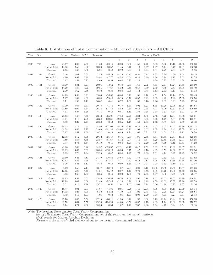
Table 8: Distribution of Total Compensation – Millions of 2005 dollars – All CEOs

Year Obs. Mean Median MAD Skewness Means by Decile

1 2 3 4 5 6 7 8 9 10

1993 715 Gross 21.57 3.09 2.95 11.50 -59.15 -0.20 0.82 1.50 2.42 3.98 5.96 10.12 21.05 230.30Net of Mkt 14.98 2.50 3.03 10.06 -80.57 -1.45 0.47 1.13 1.97 3.27 5.14 8.77 17.81 193.83Classical 2.55 1.60 0.82 5.21 0.42 0.72 0.94 1.19 1.44 1.81 2.27 2.91 4.07 9.76

1994 1,334 Gross 5.46 1.01 2.34 17.45 -46.18 -4.25 -0.75 0.31 0.74 1.37 2.28 4.00 8.04 89.28Net of Mkt 4.60 0.92 2.39 18.92 -47.77 -4.58 -0.94 0.26 0.69 1.26 2.14 3.85 7.63 83.75Classical 2.67 1.57 0.87 4.69 0.38 0.64 0.85 1.13 1.41 1.78 2.25 3.05 4.38 10.90

1995 1,401 Gross 30.70 3.81 3.71 20.95 -13.62 -0.18 0.85 1.69 2.92 4.83 7.67 13.24 24.85 265.00Net of Mkt 14.29 1.80 3.72 19.85 -47.67 -5.32 -0.49 0.58 1.30 2.50 4.38 7.87 15.05 165.40Classical 2.79 1.62 0.88 8.50 0.39 0.68 0.90 1.14 1.45 1.83 2.33 3.17 4.67 11.33

1996 1,439 Gross 24.15 3.56 3.91 19.69 -24.86 -0.64 0.72 1.51 2.76 4.51 7.54 12.14 23.54 215.43Net of Mkt 7.67 1.58 4.03 -0.84 -79.48 -5.19 -0.76 0.52 1.22 2.33 4.43 7.88 15.35 130.58Classical 3.71 1.90 1.11 16.62 0.41 0.72 1.01 1.30 1.70 2.16 2.82 3.91 5.93 17.16

1997 1,432 Gross 53.70 6.67 6.41 29.18 -41.76 0.15 1.45 3.02 5.23 8.35 13.28 22.08 41.05 484.88Net of Mkt 23.89 2.99 5.74 26.14 -111.43 -5.82 -0.61 0.86 2.08 4.01 6.96 12.71 24.05 306.69Classical 4.51 2.27 1.38 8.71 0.45 0.81 1.15 1.52 1.98 2.55 3.33 4.64 6.93 21.79

1998 1,438 Gross 70.15 1.68 6.42 23.40 -65.21 -7.54 -2.26 -0.03 1.06 2.56 5.76 12.94 34.93 723.01Net of Mkt 34.31 -0.10 7.29 23.38 -129.31 -19.09 -8.74 -3.77 -0.92 0.43 1.77 5.81 19.56 478.71Classical 5.30 2.32 1.41 28.30 0.43 0.85 1.19 1.59 2.05 2.66 3.57 4.97 7.59 28.18

1999 1,485 Gross 98.45 1.74 6.64 24.95 -177.03 -8.35 -2.18 0.14 1.11 2.67 6.57 14.45 37.96 1,112.32Net of Mkt 66.58 0.49 7.75 23.60 -281.30 -18.04 -6.73 -1.98 0.02 1.05 3.34 9.43 27.55 932.43Classical 5.87 2.51 1.58 8.57 0.43 0.89 1.24 1.66 2.21 2.92 4.01 5.81 9.12 30.58

2000 1,430 Gross -12.38 4.12 8.39 -29.32 -525.47 -8.15 -0.65 1.05 2.89 5.87 10.85 20.81 46.95 322.08Net of Mkt 1.89 4.88 8.69 -23.27 -451.67 -5.73 -0.04 1.45 3.51 6.79 12.85 23.49 52.01 375.98Classical 7.47 2.74 1.84 16.19 0.41 0.84 1.25 1.70 2.29 3.16 4.38 6.12 10.43 44.22

2001 1,396 Gross -2.00 2.08 6.26 14.37 -339.37 -12.21 -2.17 0.47 1.52 3.02 5.82 10.69 20.87 291.31Net of Mkt 23.09 3.62 6.01 20.34 -218.16 -5.33 0.15 1.47 2.76 4.99 8.51 14.90 29.31 393.06Classical 6.93 2.78 1.94 12.95 0.42 0.84 1.25 1.73 2.38 3.31 4.74 6.95 11.49 36.32

2002 1,448 Gross -20.90 0.43 4.81 -24.79 -336.86 -15.63 -5.42 -1.55 0.02 0.91 2.32 4.71 9.92 131.62Net of Mkt 12.12 2.46 4.79 -11.11 -173.41 -4.71 -0.47 0.74 1.83 3.26 5.82 10.58 20.55 257.30Classical 5.26 2.81 1.83 5.52 0.45 0.90 1.30 1.79 2.43 3.25 4.41 6.10 9.43 22.55

2003 1,522 Gross 35.02 8.56 7.14 13.17 -28.12 1.37 2.94 4.82 7.18 10.66 15.53 24.53 44.57 267.06Net of Mkt 12.63 5.82 5.42 -14.61 -95.12 0.07 1.42 2.79 4.58 7.05 10.70 16.96 31.42 146.65Classical 4.83 2.68 1.67 3.86 0.46 0.90 1.30 1.79 2.33 3.07 4.02 5.69 8.56 20.17

2004 1,517 Gross 28.85 6.54 6.51 13.48 -36.84 -0.70 1.39 2.90 5.10 8.01 12.03 18.55 32.99 246.01Net of Mkt 19.19 5.07 6.00 11.40 -57.45 -2.13 0.70 2.14 3.88 6.50 10.03 15.55 27.26 185.79Classical 5.31 3.10 1.96 5.71 0.50 1.01 1.55 2.09 2.74 3.56 4.70 6.27 9.37 21.36

2005 1,529 Gross 18.47 3.91 5.07 11.67 -45.81 -2.91 0.28 1.40 2.95 4.98 8.05 14.15 27.00 175.34Net of Mkt 14.32 3.28 5.05 6.30 -64.34 -4.19 -0.09 1.05 2.43 4.31 7.25 12.74 24.74 159.84Classical 5.42 3.16 1.97 4.06 0.53 1.05 1.53 2.08 2.79 3.65 4.63 6.21 9.37 22.33

2006 1,428 Gross 45.70 4.85 5.58 27.15 -60.11 -1.35 0.76 1.92 3.66 6.18 10.14 16.94 30.66 450.33Net of Mkt 31.55 3.04 5.55 29.90 -104.94 -4.65 -0.50 0.87 2.15 4.08 7.14 13.08 23.35 375.72Classical 6.74 3.24 2.00 38.53 0.54 1.07 1.49 2.07 2.80 3.64 4.73 6.44 9.54 35.15

Note: The heading Gross denotes Total Yearly Compensation.Net of Mkt denotes Total Yearly Compensation, net of the return on the market portfolio.MAD stands for Median Absolute Deviation.Skewness is the ratio of third moment about to the mean to the standard deviation.

32

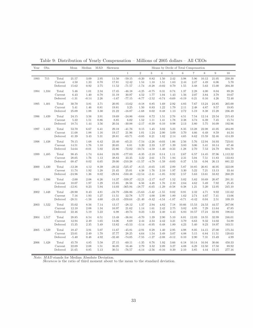
Table 9: Distribution of Yearly Compensation – Millions of 2005 dollars – All CEOs

Year Obs. Mean Median MAD Skewness Means by Decile of Total Compensation

1 2 3 4 5 6 7 8 9 10

1993 715 Total 21.57 3.09 2.95 11.50 -59.15 -0.20 0.82 1.50 2.42 3.98 5.96 10.12 21.05 230.30Current 4.50 1.33 0.70 17.81 12.42 1.54 1.10 1.51 1.63 2.44 2.47 4.49 6.06 5.70Deferred 15.62 0.92 2.75 11.52 -71.57 -1.74 -0.28 -0.02 0.79 1.55 3.48 5.63 15.00 204.30

1994 1,334 Total 5.46 1.01 2.34 17.45 -46.18 -4.25 -0.75 0.31 0.74 1.37 2.28 4.00 8.04 89.28Current 6.43 1.40 0.78 31.19 30.97 4.52 1.77 1.04 1.43 1.56 2.07 3.84 3.78 10.67Deferred -1.31 -0.14 2.26 -1.67 -77.15 -8.77 -2.52 -0.74 -0.69 -0.19 0.21 0.16 4.26 72.40

1995 1,401 Total 30.70 3.81 3.71 20.95 -13.62 -0.18 0.85 1.69 2.92 4.83 7.67 13.24 24.85 265.00Current 5.41 1.46 0.81 19.81 3.25 1.50 0.83 1.22 1.79 2.11 2.48 4.87 9.57 19.85Deferred 25.09 1.88 3.30 21.22 -16.87 -1.68 0.02 0.48 1.13 2.72 5.19 8.38 15.28 236.49

1996 1,439 Total 24.15 3.56 3.91 19.69 -24.86 -0.64 0.72 1.51 2.76 4.51 7.54 12.14 23.54 215.43Current 5.22 1.51 0.86 8.85 6.02 1.52 1.11 1.41 1.78 2.38 3.74 6.39 7.45 15.74Deferred 18.74 1.44 3.56 20.34 -30.88 -2.17 -0.39 0.10 0.98 2.13 3.80 5.75 16.09 192.96

1997 1,432 Total 53.70 6.67 6.41 29.18 -41.76 0.15 1.45 3.02 5.23 8.35 13.28 22.08 41.05 484.88Current 11.68 1.88 1.16 19.17 21.96 1.01 1.24 2.00 3.09 3.70 4.66 6.49 8.59 44.34Deferred 41.39 3.43 5.31 28.81 -63.71 -0.85 0.21 1.02 2.14 4.65 8.62 15.59 32.46 414.39

1998 1,438 Total 70.15 1.68 6.42 23.40 -65.21 -7.54 -2.26 -0.03 1.06 2.56 5.76 12.94 34.93 723.01Current 14.51 1.76 1.10 20.65 6.81 3.20 2.33 1.37 1.39 3.83 3.06 5.41 10.14 67.46Deferred 54.64 -0.01 5.92 22.86 -72.02 -10.74 -4.59 -1.40 -0.33 -1.28 2.70 7.53 24.79 604.78

1999 1,485 Total 98.45 1.74 6.64 24.95 -177.03 -8.35 -2.18 0.14 1.11 2.67 6.57 14.45 37.96 1,112.32Current 28.05 1.76 1.12 38.83 33.35 3.22 2.61 1.73 1.94 2.31 5.04 7.51 11.83 133.83Deferred 68.47 0.02 6.65 29.00 -210.38 -11.57 -4.78 -1.59 -0.83 0.37 1.53 6.94 26.13 881.22

2000 1,430 Total -12.38 4.12 8.39 -29.32 -525.47 -8.15 -0.65 1.05 2.89 5.87 10.85 20.81 46.95 322.08Current 11.74 1.92 1.28 21.45 25.01 4.38 1.76 2.10 1.97 3.30 5.22 7.21 13.13 33.44Deferred -24.96 1.36 8.02 -29.84 -550.48 -12.54 -2.41 -1.05 0.92 2.57 5.63 13.61 33.82 260.29

2001 1,396 Total -2.00 2.08 6.26 14.37 -339.37 -12.21 -2.17 0.47 1.52 3.02 5.82 10.69 20.87 291.31Current 10.07 1.97 1.29 15.85 26.56 6.56 4.48 1.76 2.10 2.64 4.62 5.49 7.92 25.45Deferred -12.81 0.23 5.94 14.03 -365.94 -18.77 -6.65 -1.29 -0.58 0.38 1.21 5.20 12.95 245.10

2002 1,448 Total -20.90 0.43 4.81 -24.79 -336.86 -15.63 -5.42 -1.55 0.02 0.91 2.32 4.71 9.92 131.62Current 7.16 1.93 1.27 11.51 22.78 5.77 4.00 2.99 1.89 1.62 2.74 4.67 7.41 13.06Deferred -28.51 -1.58 4.60 -24.43 -359.64 -21.40 -9.42 -4.54 -1.87 -0.71 -0.42 0.04 2.51 109.19

2003 1,522 Total 35.02 8.56 7.14 13.17 -28.12 1.37 2.94 4.82 7.18 10.66 15.53 24.53 44.57 267.06Current 12.10 2.08 1.34 16.97 21.62 1.14 1.61 2.42 2.75 3.82 4.95 7.29 11.64 47.85Deferred 22.46 5.19 5.22 6.98 -49.74 0.23 1.33 2.40 4.43 6.83 10.57 17.24 32.93 198.63

2004 1,517 Total 28.85 6.54 6.51 13.48 -36.84 -0.70 1.39 2.90 5.10 8.01 12.03 18.55 32.99 246.01Current 12.94 2.49 1.65 14.06 8.69 2.44 2.34 2.42 3.21 3.79 6.63 9.32 14.02 54.88Deferred 15.35 2.35 5.49 13.82 -45.53 -3.14 -0.95 0.48 1.89 4.23 5.40 9.23 18.97 163.51

2005 1,529 Total 18.47 3.91 5.07 11.67 -45.81 -2.91 0.28 1.40 2.95 4.98 8.05 14.15 27.00 175.34Current 23.01 2.49 1.70 37.77 28.25 4.64 1.54 3.49 3.07 4.88 5.15 6.84 11.51 120.63Deferred -5.40 0.48 4.92 -32.40 -74.05 -7.55 -1.27 -2.08 -0.12 0.10 2.90 7.31 15.49 4.99

2006 1,428 Total 45.70 4.85 5.58 27.15 -60.11 -1.35 0.76 1.92 3.66 6.18 10.14 16.94 30.66 450.33Current 22.09 2.08 1.51 36.05 16.46 2.79 3.32 2.09 3.27 4.08 6.29 12.50 17.50 89.92Deferred 21.65 0.85 5.13 30.51 -76.57 -4.14 -2.56 -0.16 0.39 2.10 3.85 4.44 13.15 277.16

Note: MAD stands for Median Absolute Deviation.Skewness is the ratio of third moment about to the mean to the standard deviation.

33

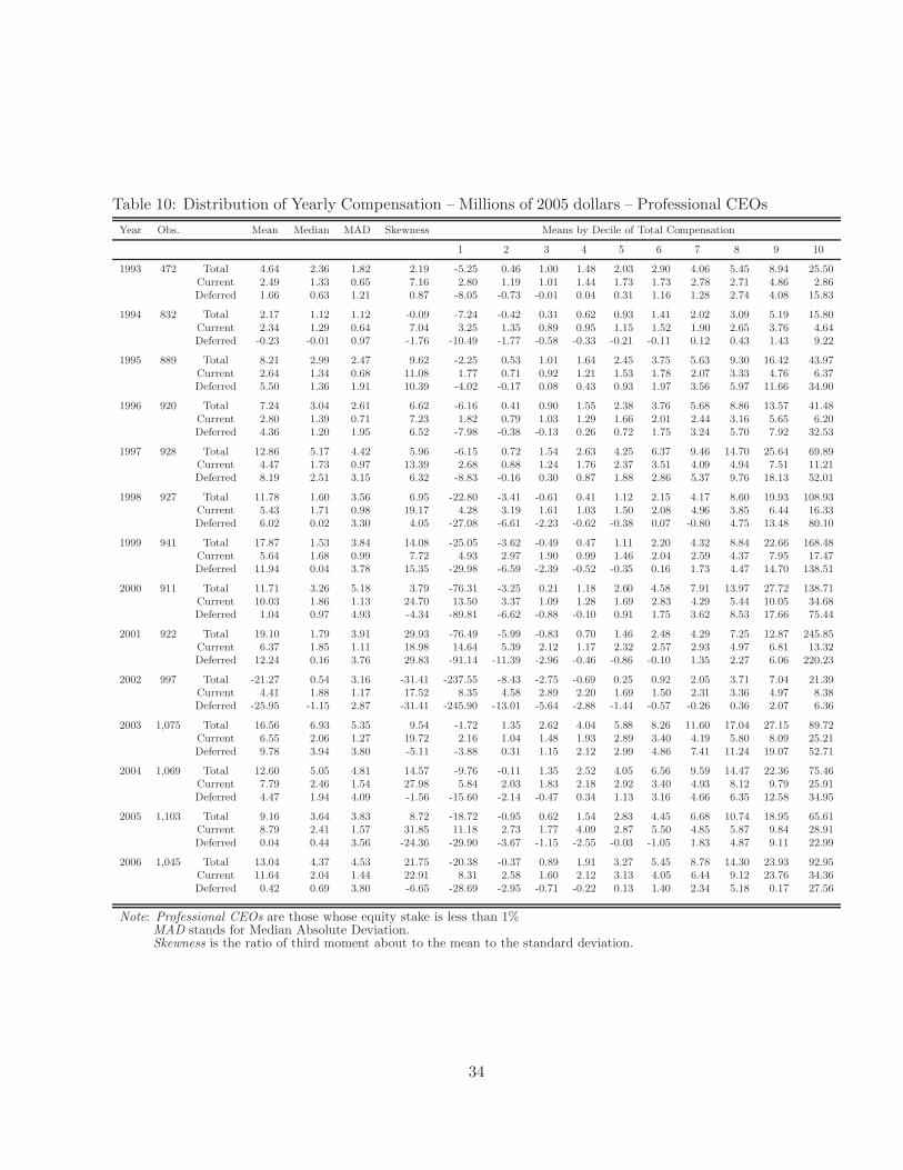
Table 10: Distribution of Yearly Compensation – Millions of 2005 dollars – Professional CEOs

Year Obs. Mean Median MAD Skewness Means by Decile of Total Compensation

1 2 3 4 5 6 7 8 9 10

1993 472 Total 4.64 2.36 1.82 2.19 -5.25 0.46 1.00 1.48 2.03 2.90 4.06 5.45 8.94 25.50Current 2.49 1.33 0.65 7.16 2.80 1.19 1.01 1.44 1.73 1.73 2.78 2.71 4.86 2.86Deferred 1.66 0.63 1.21 0.87 -8.05 -0.73 -0.01 0.04 0.31 1.16 1.28 2.74 4.08 15.83

1994 832 Total 2.17 1.12 1.12 -0.09 -7.24 -0.42 0.31 0.62 0.93 1.41 2.02 3.09 5.19 15.80Current 2.34 1.29 0.64 7.04 3.25 1.35 0.89 0.95 1.15 1.52 1.90 2.65 3.76 4.64Deferred -0.23 -0.01 0.97 -1.76 -10.49 -1.77 -0.58 -0.33 -0.21 -0.11 0.12 0.43 1.43 9.22

1995 889 Total 8.21 2.99 2.47 9.62 -2.25 0.53 1.01 1.64 2.45 3.75 5.63 9.30 16.42 43.97Current 2.64 1.34 0.68 11.08 1.77 0.71 0.92 1.21 1.53 1.78 2.07 3.33 4.76 6.37Deferred 5.50 1.36 1.91 10.39 -4.02 -0.17 0.08 0.43 0.93 1.97 3.56 5.97 11.66 34.90

1996 920 Total 7.24 3.04 2.61 6.62 -6.16 0.41 0.90 1.55 2.38 3.76 5.68 8.86 13.57 41.48Current 2.80 1.39 0.71 7.23 1.82 0.79 1.03 1.29 1.66 2.01 2.44 3.16 5.65 6.20Deferred 4.36 1.20 1.95 6.52 -7.98 -0.38 -0.13 0.26 0.72 1.75 3.24 5.70 7.92 32.53

1997 928 Total 12.86 5.17 4.42 5.96 -6.15 0.72 1.54 2.63 4.25 6.37 9.46 14.70 25.64 69.89Current 4.47 1.73 0.97 13.39 2.68 0.88 1.24 1.76 2.37 3.51 4.09 4.94 7.51 11.21Deferred 8.19 2.51 3.15 6.32 -8.83 -0.16 0.30 0.87 1.88 2.86 5.37 9.76 18.13 52.01

1998 927 Total 11.78 1.60 3.56 6.95 -22.80 -3.41 -0.61 0.41 1.12 2.15 4.17 8.60 19.93 108.93Current 5.43 1.71 0.98 19.17 4.28 3.19 1.61 1.03 1.50 2.08 4.96 3.85 6.44 16.33Deferred 6.02 0.02 3.30 4.05 -27.08 -6.61 -2.23 -0.62 -0.38 0.07 -0.80 4.75 13.48 80.10

1999 941 Total 17.87 1.53 3.84 14.08 -25.05 -3.62 -0.49 0.47 1.11 2.20 4.32 8.84 22.66 168.48Current 5.64 1.68 0.99 7.72 4.93 2.97 1.90 0.99 1.46 2.04 2.59 4.37 7.95 17.47Deferred 11.94 0.04 3.78 15.35 -29.98 -6.59 -2.39 -0.52 -0.35 0.16 1.73 4.47 14.70 138.51

2000 911 Total 11.71 3.26 5.18 3.79 -76.31 -3.25 0.21 1.18 2.60 4.58 7.91 13.97 27.72 138.71Current 10.03 1.86 1.13 24.70 13.50 3.37 1.09 1.28 1.69 2.83 4.29 5.44 10.05 34.68Deferred 1.04 0.97 4.93 -4.34 -89.81 -6.62 -0.88 -0.10 0.91 1.75 3.62 8.53 17.66 75.44

2001 922 Total 19.10 1.79 3.91 29.93 -76.49 -5.99 -0.83 0.70 1.46 2.48 4.29 7.25 12.87 245.85Current 6.37 1.85 1.11 18.98 14.64 5.39 2.12 1.17 2.32 2.57 2.93 4.97 6.81 13.32Deferred 12.24 0.16 3.76 29.83 -91.14 -11.39 -2.96 -0.46 -0.86 -0.10 1.35 2.27 6.06 220.23

2002 997 Total -21.27 0.54 3.16 -31.41 -237.55 -8.43 -2.75 -0.69 0.25 0.92 2.05 3.71 7.04 21.39Current 4.41 1.88 1.17 17.52 8.35 4.58 2.89 2.20 1.69 1.50 2.31 3.36 4.97 8.38Deferred -25.95 -1.15 2.87 -31.41 -245.90 -13.01 -5.64 -2.88 -1.44 -0.57 -0.26 0.36 2.07 6.36

2003 1,075 Total 16.56 6.93 5.35 9.54 -1.72 1.35 2.62 4.04 5.88 8.26 11.60 17.04 27.15 89.72Current 6.55 2.06 1.27 19.72 2.16 1.04 1.48 1.93 2.89 3.40 4.19 5.80 8.09 25.21Deferred 9.78 3.94 3.80 -5.11 -3.88 0.31 1.15 2.12 2.99 4.86 7.41 11.24 19.07 52.71

2004 1,069 Total 12.60 5.05 4.81 14.57 -9.76 -0.11 1.35 2.52 4.05 6.56 9.59 14.47 22.36 75.46Current 7.79 2.46 1.54 27.98 5.84 2.03 1.83 2.18 2.92 3.40 4.93 8.12 9.79 25.91Deferred 4.47 1.94 4.09 -1.56 -15.60 -2.14 -0.47 0.34 1.13 3.16 4.66 6.35 12.58 34.95

2005 1,103 Total 9.16 3.64 3.83 8.72 -18.72 -0.95 0.62 1.54 2.83 4.45 6.68 10.74 18.95 65.61Current 8.79 2.41 1.57 31.85 11.18 2.73 1.77 4.09 2.87 5.50 4.85 5.87 9.84 28.91Deferred 0.04 0.44 3.56 -24.36 -29.90 -3.67 -1.15 -2.55 -0.03 -1.05 1.83 4.87 9.11 22.99

2006 1,045 Total 13.04 4.37 4.53 21.75 -20.38 -0.37 0.89 1.91 3.27 5.45 8.78 14.30 23.93 92.95Current 11.64 2.04 1.44 22.91 8.31 2.58 1.60 2.12 3.13 4.05 6.44 9.12 23.76 34.36Deferred 0.42 0.69 3.80 -6.65 -28.69 -2.95 -0.71 -0.22 0.13 1.40 2.34 5.18 0.17 27.56

Note: Professional CEOs are those whose equity stake is less than 1%MAD stands for Median Absolute Deviation.Skewness is the ratio of third moment about to the mean to the standard deviation.

34

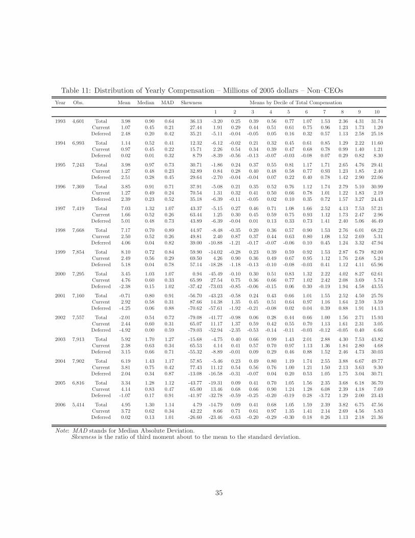
Table 11: Distribution of Yearly Compensation – Millions of 2005 dollars – Non–CEOs

Year Obs. Mean Median MAD Skewness Means by Decile of Total Compensation

1 2 3 4 5 6 7 8 9 10

1993 4,601 Total 3.98 0.90 0.64 36.13 -3.20 0.25 0.39 0.56 0.77 1.07 1.53 2.36 4.31 31.74Current 1.07 0.45 0.21 27.44 1.91 0.29 0.44 0.51 0.61 0.75 0.96 1.23 1.73 1.20Deferred 2.48 0.20 0.42 35.21 -5.11 -0.04 -0.05 0.05 0.16 0.32 0.57 1.13 2.58 25.18

1994 6,993 Total 1.14 0.52 0.41 12.32 -6.12 -0.02 0.21 0.32 0.45 0.61 0.85 1.29 2.22 11.60Current 0.97 0.45 0.22 15.71 2.26 0.54 0.34 0.39 0.47 0.68 0.78 0.99 1.40 1.21Deferred 0.02 0.01 0.32 8.79 -8.39 -0.56 -0.13 -0.07 -0.03 -0.08 0.07 0.29 0.82 8.30

1995 7,243 Total 3.98 0.97 0.73 30.71 -1.86 0.24 0.37 0.55 0.81 1.17 1.71 2.65 4.76 29.41Current 1.27 0.48 0.23 32.89 0.84 0.28 0.40 0.48 0.58 0.77 0.93 1.23 1.85 2.40Deferred 2.51 0.28 0.45 29.64 -2.70 -0.04 -0.04 0.07 0.22 0.40 0.78 1.42 2.90 22.06

1996 7,369 Total 3.85 0.91 0.71 37.91 -5.08 0.21 0.35 0.52 0.76 1.12 1.74 2.79 5.10 30.99Current 1.27 0.49 0.24 70.54 1.31 0.32 0.41 0.50 0.66 0.78 1.01 1.22 1.83 2.19Deferred 2.39 0.23 0.52 35.18 -6.39 -0.11 -0.05 0.02 0.10 0.35 0.72 1.57 3.27 24.43

1997 7,419 Total 7.03 1.32 1.07 43.37 -5.15 0.27 0.46 0.71 1.08 1.66 2.52 4.13 7.53 57.21Current 1.66 0.52 0.26 63.44 1.25 0.30 0.45 0.59 0.75 0.93 1.12 1.73 2.47 2.96Deferred 5.01 0.48 0.73 43.89 -6.39 -0.04 0.01 0.13 0.33 0.73 1.41 2.40 5.06 46.49

1998 7,668 Total 7.17 0.70 0.89 44.97 -8.48 -0.35 0.20 0.36 0.57 0.90 1.53 2.76 6.01 68.22Current 2.50 0.52 0.26 49.81 2.40 0.87 0.37 0.44 0.63 0.80 1.08 1.52 2.69 5.31Deferred 4.06 0.04 0.82 39.00 -10.88 -1.21 -0.17 -0.07 -0.06 0.10 0.45 1.24 3.32 47.94

1999 7,854 Total 8.10 0.72 0.84 59.90 -14.02 -0.28 0.23 0.39 0.59 0.92 1.53 2.87 6.79 82.00Current 2.49 0.56 0.29 69.50 4.26 0.90 0.36 0.49 0.67 0.95 1.12 1.76 2.68 5.24Deferred 5.18 0.04 0.78 57.14 -18.28 -1.18 -0.13 -0.10 -0.08 -0.03 0.41 1.12 4.11 65.96

2000 7,295 Total 3.45 1.03 1.07 0.94 -45.49 -0.10 0.30 0.51 0.83 1.32 2.22 4.02 8.27 62.61Current 4.76 0.60 0.33 65.99 27.54 0.75 0.36 0.66 0.77 1.02 2.42 2.08 3.69 5.74Deferred -2.38 0.15 1.02 -37.42 -73.03 -0.85 -0.06 -0.15 0.06 0.30 -0.19 1.94 4.58 43.55

2001 7,160 Total -0.71 0.80 0.91 -56.70 -43.23 -0.58 0.24 0.43 0.66 1.01 1.55 2.52 4.50 25.76Current 2.92 0.58 0.31 87.66 14.38 1.35 0.45 0.51 0.64 0.97 1.16 1.64 2.59 3.59Deferred -4.25 0.06 0.88 -70.62 -57.61 -1.92 -0.21 -0.08 0.02 0.04 0.39 0.88 1.91 14.13

2002 7,557 Total -2.01 0.54 0.72 -79.08 -41.77 -0.98 0.06 0.28 0.44 0.66 1.00 1.56 2.71 15.93Current 2.44 0.60 0.31 65.07 11.17 1.37 0.59 0.42 0.55 0.70 1.13 1.61 2.31 3.05Deferred -4.92 0.00 0.59 -79.03 -52.94 -2.35 -0.53 -0.14 -0.11 -0.03 -0.12 -0.05 0.40 6.66

2003 7,913 Total 5.92 1.70 1.27 -15.68 -4.75 0.40 0.66 0.99 1.43 2.01 2.88 4.30 7.53 43.82Current 2.38 0.63 0.34 65.53 4.14 0.41 0.57 0.70 0.97 1.13 1.36 1.84 2.80 4.68Deferred 3.15 0.66 0.71 -55.32 -8.89 -0.01 0.09 0.29 0.46 0.88 1.52 2.46 4.73 30.03

2004 7,902 Total 6.19 1.43 1.17 57.85 -5.46 0.23 0.49 0.80 1.19 1.74 2.55 3.88 6.67 49.77Current 3.81 0.75 0.42 77.43 11.12 0.54 0.56 0.76 1.00 1.21 1.50 2.13 3.63 9.30Deferred 2.04 0.34 0.87 -13.08 -16.58 -0.31 -0.07 0.04 0.20 0.53 1.05 1.75 3.04 30.71

2005 6,816 Total 3.34 1.28 1.12 -43.77 -19.31 0.09 0.41 0.70 1.05 1.56 2.35 3.68 6.18 36.70Current 4.14 0.83 0.47 65.00 13.46 0.68 0.66 0.90 1.24 1.28 6.08 2.39 4.18 7.69Deferred -1.07 0.17 0.91 -41.97 -32.78 -0.59 -0.25 -0.20 -0.19 0.28 -3.72 1.29 2.00 23.43

2006 5,414 Total 4.95 1.30 1.14 4.79 -14.79 0.09 0.41 0.68 1.05 1.59 2.39 3.82 6.75 47.56Current 3.72 0.62 0.34 42.22 8.66 0.71 0.61 0.97 1.35 1.41 2.14 2.69 4.56 5.83Deferred 0.02 0.13 1.01 -26.60 -23.46 -0.63 -0.20 -0.29 -0.30 0.18 0.26 1.13 2.18 21.36

Note: MAD stands for Median Absolute Deviation.Skewness is the ratio of third moment about to the mean to the standard deviation.

35

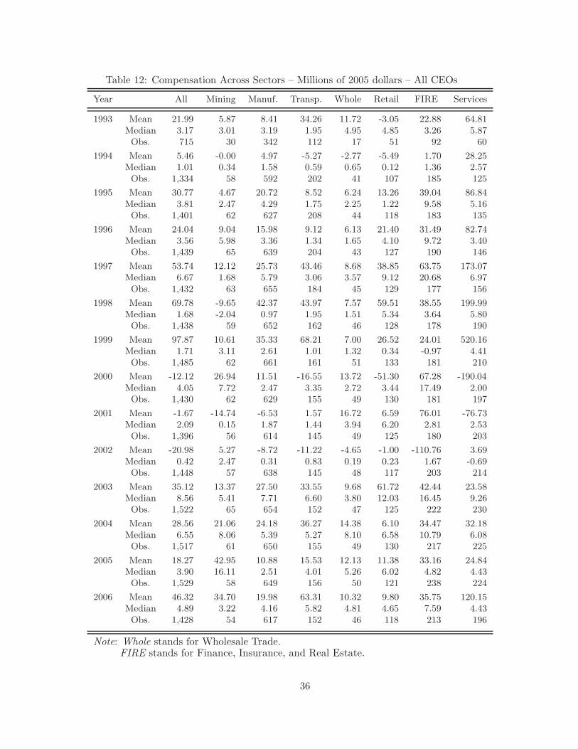
Table 12: Compensation Across Sectors – Millions of 2005 dollars – All CEOs

Year All Mining Manuf. Transp. Whole Retail FIRE Services

1993 Mean 21.99 5.87 8.41 34.26 11.72 -3.05 22.88 64.81Median 3.17 3.01 3.19 1.95 4.95 4.85 3.26 5.87Obs. 715 30 342 112 17 51 92 60

1994 Mean 5.46 -0.00 4.97 -5.27 -2.77 -5.49 1.70 28.25Median 1.01 0.34 1.58 0.59 0.65 0.12 1.36 2.57Obs. 1,334 58 592 202 41 107 185 125

1995 Mean 30.77 4.67 20.72 8.52 6.24 13.26 39.04 86.84Median 3.81 2.47 4.29 1.75 2.25 1.22 9.58 5.16Obs. 1,401 62 627 208 44 118 183 135

1996 Mean 24.04 9.04 15.98 9.12 6.13 21.40 31.49 82.74Median 3.56 5.98 3.36 1.34 1.65 4.10 9.72 3.40Obs. 1,439 65 639 204 43 127 190 146

1997 Mean 53.74 12.12 25.73 43.46 8.68 38.85 63.75 173.07Median 6.67 1.68 5.79 3.06 3.57 9.12 20.68 6.97Obs. 1,432 63 655 184 45 129 177 156

1998 Mean 69.78 -9.65 42.37 43.97 7.57 59.51 38.55 199.99Median 1.68 -2.04 0.97 1.95 1.51 5.34 3.64 5.80Obs. 1,438 59 652 162 46 128 178 190

1999 Mean 97.87 10.61 35.33 68.21 7.00 26.52 24.01 520.16Median 1.71 3.11 2.61 1.01 1.32 0.34 -0.97 4.41Obs. 1,485 62 661 161 51 133 181 210

2000 Mean -12.12 26.94 11.51 -16.55 13.72 -51.30 67.28 -190.04Median 4.05 7.72 2.47 3.35 2.72 3.44 17.49 2.00Obs. 1,430 62 629 155 49 130 181 197

2001 Mean -1.67 -14.74 -6.53 1.57 16.72 6.59 76.01 -76.73Median 2.09 0.15 1.87 1.44 3.94 6.20 2.81 2.53Obs. 1,396 56 614 145 49 125 180 203

2002 Mean -20.98 5.27 -8.72 -11.22 -4.65 -1.00 -110.76 3.69Median 0.42 2.47 0.31 0.83 0.19 0.23 1.67 -0.69Obs. 1,448 57 638 145 48 117 203 214

2003 Mean 35.12 13.37 27.50 33.55 9.68 61.72 42.44 23.58Median 8.56 5.41 7.71 6.60 3.80 12.03 16.45 9.26Obs. 1,522 65 654 152 47 125 222 230

2004 Mean 28.56 21.06 24.18 36.27 14.38 6.10 34.47 32.18Median 6.55 8.06 5.39 5.27 8.10 6.58 10.79 6.08Obs. 1,517 61 650 155 49 130 217 225

2005 Mean 18.27 42.95 10.88 15.53 12.13 11.38 33.16 24.84Median 3.90 16.11 2.51 4.01 5.26 6.02 4.82 4.43Obs. 1,529 58 649 156 50 121 238 224

2006 Mean 46.32 34.70 19.98 63.31 10.32 9.80 35.75 120.15Median 4.89 3.22 4.16 5.82 4.81 4.65 7.59 4.43Obs. 1,428 54 617 152 46 118 213 196

Note: Whole stands for Wholesale Trade.FIRE stands for Finance, Insurance, and Real Estate.

36

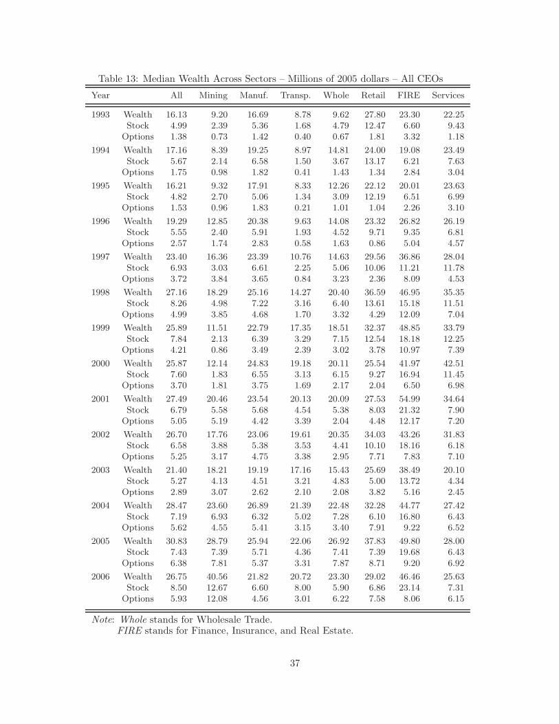
Table 13: Median Wealth Across Sectors – Millions of 2005 dollars – All CEOs

Year All Mining Manuf. Transp. Whole Retail FIRE Services

1993 Wealth 16.13 9.20 16.69 8.78 9.62 27.80 23.30 22.25Stock 4.99 2.39 5.36 1.68 4.79 12.47 6.60 9.43

Options 1.38 0.73 1.42 0.40 0.67 1.81 3.32 1.18

1994 Wealth 17.16 8.39 19.25 8.97 14.81 24.00 19.08 23.49Stock 5.67 2.14 6.58 1.50 3.67 13.17 6.21 7.63

Options 1.75 0.98 1.82 0.41 1.43 1.34 2.84 3.04

1995 Wealth 16.21 9.32 17.91 8.33 12.26 22.12 20.01 23.63Stock 4.82 2.70 5.06 1.34 3.09 12.19 6.51 6.99

Options 1.53 0.96 1.83 0.21 1.01 1.04 2.26 3.10

1996 Wealth 19.29 12.85 20.38 9.63 14.08 23.32 26.82 26.19Stock 5.55 2.40 5.91 1.93 4.52 9.71 9.35 6.81

Options 2.57 1.74 2.83 0.58 1.63 0.86 5.04 4.57

1997 Wealth 23.40 16.36 23.39 10.76 14.63 29.56 36.86 28.04Stock 6.93 3.03 6.61 2.25 5.06 10.06 11.21 11.78

Options 3.72 3.84 3.65 0.84 3.23 2.36 8.09 4.53

1998 Wealth 27.16 18.29 25.16 14.27 20.40 36.59 46.95 35.35Stock 8.26 4.98 7.22 3.16 6.40 13.61 15.18 11.51

Options 4.99 3.85 4.68 1.70 3.32 4.29 12.09 7.04

1999 Wealth 25.89 11.51 22.79 17.35 18.51 32.37 48.85 33.79Stock 7.84 2.13 6.39 3.29 7.15 12.54 18.18 12.25

Options 4.21 0.86 3.49 2.39 3.02 3.78 10.97 7.39

2000 Wealth 25.87 12.14 24.83 19.18 20.11 25.54 41.97 42.51Stock 7.60 1.83 6.55 3.13 6.15 9.27 16.94 11.45

Options 3.70 1.81 3.75 1.69 2.17 2.04 6.50 6.98

2001 Wealth 27.49 20.46 23.54 20.13 20.09 27.53 54.99 34.64Stock 6.79 5.58 5.68 4.54 5.38 8.03 21.32 7.90

Options 5.05 5.19 4.42 3.39 2.04 4.48 12.17 7.20

2002 Wealth 26.70 17.76 23.06 19.61 20.35 34.03 43.26 31.83Stock 6.58 3.88 5.38 3.53 4.41 10.10 18.16 6.18

Options 5.25 3.17 4.75 3.38 2.95 7.71 7.83 7.10

2003 Wealth 21.40 18.21 19.19 17.16 15.43 25.69 38.49 20.10Stock 5.27 4.13 4.51 3.21 4.83 5.00 13.72 4.34

Options 2.89 3.07 2.62 2.10 2.08 3.82 5.16 2.45

2004 Wealth 28.47 23.60 26.89 21.39 22.48 32.28 44.77 27.42Stock 7.19 6.93 6.32 5.02 7.28 6.10 16.80 6.43

Options 5.62 4.55 5.41 3.15 3.40 7.91 9.22 6.52

2005 Wealth 30.83 28.79 25.94 22.06 26.92 37.83 49.80 28.00Stock 7.43 7.39 5.71 4.36 7.41 7.39 19.68 6.43

Options 6.38 7.81 5.37 3.31 7.87 8.71 9.20 6.92

2006 Wealth 26.75 40.56 21.82 20.72 23.30 29.02 46.46 25.63Stock 8.50 12.67 6.60 8.00 5.90 6.86 23.14 7.31

Options 5.93 12.08 4.56 3.01 6.22 7.58 8.06 6.15

Note: Whole stands for Wholesale Trade.FIRE stands for Finance, Insurance, and Real Estate.

37

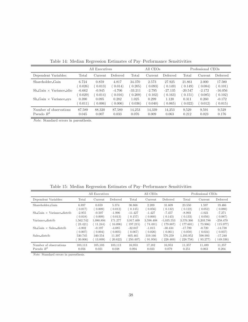
Table 14: Median Regression Estimates of Pay–Performance Sensitivities

All Executives All CEOs Professional CEOs

Dependent Variables: Total Current Deferred Total Current Deferred Total Current Deferred

Shareholder Gain 6.724 0.859 4.817 34.370 2.573 27.925 21.861 2.000 17.580( 0.026) ( 0.013) ( 0.014) ( 0.205) ( 0.093) ( 0.149) ( 0.149) ( 0.084) ( 0.101)

Sh Gain ! Variance idio -6.662 -0.945 -4.706 -33.211 -2.795 -27.135 -20.547 -2.172 -16.056( 0.029) ( 0.014) ( 0.016) ( 0.209) ( 0.102) ( 0.163) ( 0.151) ( 0.085) ( 0.102)

Sh Gain ! Variance sys 0.390 0.095 0.282 1.025 0.299 1.120 0.311 0.260 -0.172( 0.011) ( 0.006) ( 0.006) ( 0.036) ( 0.040) ( 0.065) ( 0.022) ( 0.012) ( 0.015)

Number of observations 87,589 88,320 87,589 14,253 14,339 14,253 9,529 9,591 9,529Pseudo R

2 0.045 0.007 0.033 0.076 0.009 0.063 0.212 0.023 0.176

Note: Standard errors in parenthesis.

Table 15: Median Regression Estimates of Pay–Performance Sensitivities

All Executives All CEOs Professional CEOs

Dependent Variables: Total Current Deferred Total Current Deferred Total Current Deferred

Shareholder Gain 6.897 0.659 5.374 36.866 2.209 31.609 23.550 1.597 19.466( 0.017) ( 0.009) ( 0.012) ( 0.145) ( 0.056) ( 0.132) ( 0.122) ( 0.052) ( 0.080)

Sh Gain ! Variance distrib -2.955 -0.507 -1.996 -11.427 -1.427 -7.457 -8.993 -1.021 -7.271( 0.018) ( 0.009) ( 0.013) ( 0.157) ( 0.060) ( 0.143) ( 0.133) ( 0.056) ( 0.087)

Variance distrib 1,562.742 1,080.894 171.277 3,917.409 3,598.408 -1,035.553 3,576.366 3,203.788 -258.470( 23.421) ( 11.244) ( 16.096) ( 197.215) ( 74.491) ( 179.887) ( 177.601) ( 73.906) ( 115.977)

Sh Gain ! Sales distrib -4.802 -0.197 -4.085 -32.047 -1.015 -30.434 -17.789 -0.720 -14.738( 0.007) ( 0.004) ( 0.005) ( 0.067) ( 0.026) ( 0.061) ( 0.058) ( 0.024) ( 0.037)

Sales distrib 530.745 340.554 11.397 605.461 319.166 576.259 1,193.952 598.993 -17.240( 30.006) ( 13.899) ( 20.622) ( 250.497) ( 91.950) ( 228.469) ( 228.758) ( 93.277) ( 149.336)

Number of observations 103,113 105,103 103,113 16,953 17,182 16,953 11,357 11,489 11,357Pseudo R

2 0.056 0.021 0.038 0.094 0.023 0.079 0.251 0.063 0.204

Note: Standard errors in parenthesis.

38