Excursions of a normal random walk above a boundary

Statistics & Probability Letters 48 (2000) 141–151

Excursions of a normal random walk above a boundary(

Evan Fishera ; ∗, Matthew Bermanb, Natalie Vowelsc, Christine Wilsond

aDepartment of Mathematics, Lafayette College, Easton, PA 18042-1781, USAbMassachusetts Institute of Technology, Cambridge, MA 02139, USA

cUniversity of San Diego, San Diego, CA 92110, USAdVillanova University, Villanova, PA 19085, USA

Received April 1999

Abstract

An integral condition is derived that is equivalent to the condition that the expected number of excursions by a normalrandom walk beyond a boundary is �nite. In the case where the expected number of excursions is in�nite, the asymptoticsize is determined relative to the number of steps. Applications are given and the behavior for a transitional family ofboundaries is investigated. c© 2000 Elsevier Science B.V. All rights reserved

Keywords: Random walks; Excursions; Boundary crossings

1. Introduction

Let {Xi; i = 1; 2; 3; : : :} be a sequence of independent, normally distributed random variables with commonmean � and common variance �2. De�ne S0 ≡ 0 and for n=1; 2; 3; : : : de�ne Sn=

∑ni=1 Xi. Suppose g : N→

[0;∞) is a non-negative increasing function (de�ne g(0) ≡ 0).We say a normal random walk {Sn; n= 1; 2; 3; : : :} begins an excursion above g at index n (n= 1; 2; 3; : : :)

if

Sn−1 − (n− 1)�6g(n− 1); Sn − n�¿g(n):

In the present context, let the function h be non-negative and monotone increasing for x¿x0 for somex0¿1. (Without loss of generality, we can assume x0 = 1 by de�ning h(x) ≡ h(x0) for 16x6x0 if x0¿ 1.)De�ne g by g(n) = �

√nh(n) for n= 1; 2; 3; : : : . For n= 1; 2; 3; : : : ; de�ne the event An by

An = (Sn − n�¿g(n); Sn+1 − (n+ 1)�6g(n+ 1)):

( This research was supported in part by NSF-REU grant DMS 9424098. The last three authors were participants in the NSF-REUprogram held at Lafayette Collete, Summer 1997.

∗ Corresponding author. Tel.: +1-610-250-5281.E-mail address: �[email protected] (E. Fisher)

0167-7152/00/$ - see front matter c© 2000 Elsevier Science B.V. All rights reservedPII: S0167 -7152(99)00196 -0

142 E. Fisher et al. / Statistics & Probability Letters 48 (2000) 141–151

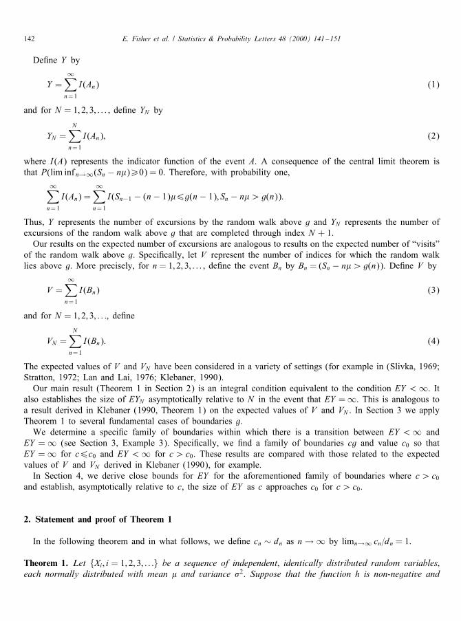
De�ne Y by

Y =∞∑n=1

I(An) (1)

and for N = 1; 2; 3; : : : ; de�ne YN by

YN =N∑n=1

I(An); (2)

where I(A) represents the indicator function of the event A. A consequence of the central limit theorem isthat P(lim inf n→∞(Sn − n�)¿0) = 0. Therefore, with probability one,

∞∑n=1

I(An) =∞∑n=1

I(Sn−1 − (n− 1)�6g(n− 1); Sn − n�¿g(n)):

Thus, Y represents the number of excursions by the random walk above g and YN represents the number ofexcursions of the random walk above g that are completed through index N + 1.Our results on the expected number of excursions are analogous to results on the expected number of “visits”

of the random walk above g. Speci�cally, let V represent the number of indices for which the random walklies above g. More precisely, for n= 1; 2; 3; : : : ; de�ne the event Bn by Bn = (Sn − n�¿g(n)). De�ne V by

V =∞∑n=1

I(Bn) (3)

and for N = 1; 2; 3; : : :, de�ne

VN =N∑n=1

I(Bn): (4)

The expected values of V and VN have been considered in a variety of settings (for example in (Slivka, 1969;Stratton, 1972; Lan and Lai, 1976; Klebaner, 1990).Our main result (Theorem 1 in Section 2) is an integral condition equivalent to the condition EY ¡∞. It

also establishes the size of EYN asymptotically relative to N in the event that EY =∞. This is analogous toa result derived in Klebaner (1990, Theorem 1) on the expected values of V and VN . In Section 3 we applyTheorem 1 to several fundamental cases of boundaries g.We determine a speci�c family of boundaries within which there is a transition between EY ¡∞ and

EY =∞ (see Section 3, Example 3). Speci�cally, we �nd a family of boundaries cg and value c0 so thatEY =∞ for c6c0 and EY ¡∞ for c¿c0. These results are compared with those related to the expectedvalues of V and VN derived in Klebaner (1990), for example.In Section 4, we derive close bounds for EY for the aforementioned family of boundaries where c¿c0

and establish, asymptotically relative to c, the size of EY as c approaches c0 for c¿c0.

2. Statement and proof of Theorem 1

In the following theorem and in what follows, we de�ne cn ∼ dn as n→ ∞ by limn→∞ cn=dn = 1.

Theorem 1. Let {Xi; i = 1; 2; 3; : : :} be a sequence of independent; identically distributed random variables;each normally distributed with mean � and variance �2. Suppose that the function h is non-negative and

E. Fisher et al. / Statistics & Probability Letters 48 (2000) 141–151 143

monotone increasing for x¿x0 for some x0¿1. De�ne the random variable Y as in (1) and the randomvariable YN as in (2). Then

EY ¡∞ i�∫ ∞

1

1√xe−h

2(x)=2 dx¡∞:

If∫∞1 (1=

√x)e−h

2(x)=2 dx =∞; then

EYN ∼ 12�

∫ N

1

1√xe−h

2(x)=2 dx

as N → ∞.

Proof. Suppose that for each i = 1; 2; 3; : : :, Xi has a normal distribution with mean � and variance �2. Foreach n=1; 2; 3; : : : , let Sn=

∑ni=1 Xi. Note that if each Xi has a normal distribution, then the random variable

X ′i = (Xi − �)=� has a standard normal distribution. If S ′n is de�ned by S ′n =

∑ni=1 X

′i , then the event

(Sn − n�¿�√nh(n); Sn+1 − (n+ 1)�6�

√n+ 1h(n+ 1))

is equivalent to the event

(S ′n ¿√nh(n); S ′n+16

√n+ 1h(n+ 1)):

Thus, Theorem 1 will be proved once it is established in the case where Xi is assumed to have a standardnormal distribution. Hence, we assume that Xi has a standard normal distribution for each i = 1; 2; 3; : : : .Without loss of generality, assume that x0 = 1 (see Section 1).We note that

P(Sn ¿√nh(n); Sn+16

√n+ 1h(n+ 1))

6P(√nh(n)¡Sn6

√nh(n+ 1); Xn+16

√n+ 1h(n+ 1)−√

nh(n))

+P(Sn ¿√nh(n+ 1); Sn+16

√n+ 1h(n+ 1)):

This yields


√n+ 1h(n+ 1))

6P(√nh(n)¡Sn6

√nh(n+ 1)) + P(Sn ¿

√nh(n+ 1); Sn+16

√n+ 1h(n+ 1)): (5)

For n= 1; 2; 3; : : :, de�ne an by

an = P(Sn ¿√nh(n+ 1); Sn+16

√n+ 1h(n+ 1)): (6)

It follows from (5) and the monotonicity of h that

EYN =N∑n=1


√n+ 1h(n+ 1))

6N∑n=1

[�(h(n+ 1))− �(h(n))] +N∑n=1

an

612+

N∑n=1

an; (7)

where �(·) represents the standard normal distribution function.


For n= 1; 2; 3; : : : , de�ne bn by

bn = (√n+ 1−√

n)h(n+ 1): (8)

Then

an =∫ bn

−∞

(�(√

n+ 1h(n+ 1)− y√n

)− �(h(n+ 1))

)�(y) dy; (9)

where �(·) represents the standard normal density function.From (9) and an application of the mean value theorem we obtain

an61√2�n

e−h2(n+1)=2

[bn�(bn) +

1√2�e−b

2n=2]: (10)

Let �¿ 0 and let A be the set of indices de�ned by

A= {n∈N: h(n+ 1)¿�√n}: (11)

From de�nition, (6), of an and a standard tail probability estimate for the standard normal distribution (seeFeller, 1968), we note that for n∈A,

an61− �(h(n+ 1))6 1√2�n�

e−�2n=2:

Therefore,

∑n∈A

an6∞∑n=1

1√2�n�

e−�2n=2¡∞: (12)

For n= 1; 2; 3; : : : ; bn ¡h(n+ 1)=(2√n). Therefore, if n 6∈ A, then bn ¡ �=2. Thus,∑

n 6∈Aan6

∑n 6∈A

1√2�n

e−h2(n+1)=2

[bn�(bn) +

1√2�e−b

2n=2]

6∑n 6∈A

1√2�n

e−h2(n+1)=2

[�+

1√2�

]: (13)

Suppose that∫∞1 (1=

√x)e−h

2(x)=2 dx¡∞. Then ∑∞n=1(1=

√n)e−h

2(n)=2¡∞ and it follows from (13) that∑n 6∈A

an ¡∞: (14)

We conclude from (7), (12), and (14) that if∫∞1 (1=

√x)e−h

2(x)=2 dx¡∞, thenEY ¡∞: (15)

For the remainder of the proof we assume that∫∞1 (1=

√x)e−h

2(x)=2 dx =∞. Then∫ N

1

1√xe−h

2(x)=2 dx ∼N∑n=1

1√ne−h

2(n)=2 ∼N∑n=1

1√ne−h

2(n+1)=2 (16)

as N → ∞.It follows from (7), (12), (13), and (16) that for every �¿ 0,

lim supN→∞

EYN

/N∑n=1

12�

√ne−h

2(n)=26√2��+ 1:


Therefore, if∫∞1 (1=

√x)e−h(x)

2=2 dx =∞, the latter inequality and (16) yield the result

lim supN→∞

EYN∫ N1 (1=2�

√x)e−h2(x)=2 dx

61: (17)

We now establish a lower bound analogous to (17). Using the de�nition, (8), of bn, we obtain


√n+ 1h(n+ 1))

¿P(√nh(n)¡Sn6

√nh(n+ 1); Xn+16bn)

+P(Sn ¿√nh(n+ 1); Sn+16

√n+ 1h(n+ 1)):

Thus,


√n+ 1h(n+ 1))

¿(�(h(n+ 1))− �(h(n)))�(0) + P(Sn ¿√nh(n+ 1); Sn+16

√n+ 1h(n+ 1)):

Therefore,

EYN¿N∑n=1

[�(h(n+ 1))− �(h(n))]�(0) +N∑n=1

an: (18)

From (9) and an application of the mean value theorem it follows that

an¿∫ bn

−∞

bn − y√n�(√

n+ 1h(n+ 1)− y√n

)�(y) dy

=1

2�√ne−h

2(n+1)=2∫ bn

−∞(bn − y)e−(h(n+1)−

√n+1y)2=2n dy:

We apply the change of variables v= (h(n+ 1)−√n+ 1y)=

√n to the latter integral and obtain

an¿1

2�√ne−h

2(n+1)=2 nn+ 1

∫ ∞

bn(v− bn)e−v2=2 dv

=1

2�√ne−h

2(n+1)=2 nn+ 1

[∫ ∞

bnve−v

2=2 dv− bn√2�(1− �(bn))

]

=1

2�√ne−h

2(n+1)=2 nn+ 1

[e−b2n=2 − bn

√2�(1− �(bn))]: (19)

The de�nition, (11), of the set of indices A leads to the inequality

∑n∈A

12�

√ne−h

2(n+1)=26∞∑n=1

12�

√ne−�

2n=2¡∞:

Since∑∞

n=1(1=2�√n)e−h

2(n+1)=2 =∞ (see (16)), then

∑n6Nn 6∈A

12�

√ne−h

2(n+1)=2 ∼N∑n=1

12�

√ne−h

2(n+1)=2 (20)

as N → ∞.


If n 6∈ A, then 0¡bn¡�=2. Therefore,

lim infN→∞

∑n6Nn 6∈A

(1=2�√n)e−h

2(n+1)=2[n=(n+ 1)][e−b2n=2 − bn

√2�(1− �(bn))]∑

n6Nn 6∈A

(1=2�√n)e−h2(n+1)=2

¿[e−�2=8 −

√2��]: (21)

By (20) and (21), we obtain

lim infN→∞

∑n6Nn 6∈A

(1=2�√n)e−h

2(n+1)=2[n=(n+ 1)][e−b2n=2 − bn

√2�(1− �(bn))]∑N

n=1(1=2�√n)e−h2(n+1)=2

¿e−�2=8 −

√2��: (22)

We recall (18) and observe that

EYN¿N∑n=1

[�(h(n+ 1))− �(h(n))]�(0) +∑n6Nn∈A

an +∑n6Nn 6∈A

an: (23)

Clearly,∑N

n=1 [�(h(n+1))−�(h(n))])�(0)¡∞. Note that ∑n∈A an ¡∞ (see (12)). It follows from (16),(22), and (23) that for all �¿ 0,

lim infN→∞

EYN∫ N1 (1=2�

√x)e−h2(x)=2 dx

¿e−�2=8 −

√2��:

Hence,

lim infN→∞

EYN∫ N1 (1=2�

√x)e−h2(x)=2 dx

¿1: (24)

The full conclusion of the theorem follows from (15), (17), and (24).

3. Application of Theorem 1

Example 1. Consider the boundary associated with the central limit theorem: let c¿ 0 and h(x)=c for x¿1.Hence, g(n) = c�

√n for n= 0; 1; 2; : : : . A simple application of Theorem 1 yields

EYN ∼ 1�√Ne−c

2=2

as N→∞.Recall the de�nition of VN (see (4)). In Klebaner (1990) it is shown that, in this setting, EVN ∼

(1=c√2�)Ne−c2=2 as N→∞. Hence the expected number of visits above the square root boundary is, asymptot-

ically, proportional to the number of steps; the expected number of excursions is, asymptotically, proportionalto the square root of the number of steps.

Example 2. Consider the boundary associated with the Hartman–Wintner law of the iterated logarithm. Thatis, for c¿ 0, let h(x) = c

√log(log x) for x¿3. From the law of the iterated logarithm (see, for example,

Stout, 1974, p. 293), it follows that for V as de�ned by (3), V ¡∞ when c¿√2 and V =∞ when c6

√2.

Nevertheless, it is shown in Slivka (1969) that EV =∞ for all c¿ 0. It follows from Theorem 1 that

EYN ∼√N

�(logN )c2=2

as N→∞.


Example 3. In the setting described by the hypotheses of Theorem 1, it has been shown (see Klebaner, 1990,p. 208; Lan and Lai, 1976, Theorem 2) that the family of boundaries described by g(n)=c�

√n log n for c¿ 0

and n = 1; 2; 3; : : : , serves as a transitional family for EV . Speci�cally, EV =∞ when c6√2 and EV ¡∞

when c¿√2.

It follows from Theorem 1 that a transitional family of boundaries for EY is the same as the aforementionedfamily for EV . However, here EY =∞ when c61 and EY ¡∞ when c¿ 1. Hence, for each 16c¡

√2

and for g(n)=c�√n log n for n=1; 2; 3; : : : ; the expected number of excursions above the boundary g is �nite

while the expected number of visits above the boundary g is in�nite.Theorem 1 also yields the following asymptotic results:

EYN ∼

12� logN if c = 1;

1�(1− c2)N

(1−c2)=2 if c¡ 1:

We consider the case c¿ 1 in the next section.

4. The family of boundaries c�√n log n for c¿ 1

Example 3 in the previous section includes the result that EY ¡∞ for boundaries of the form g(n) =c�

√n log n for c¿ 1. In this section we derive close upper and lower bounds for EY and characterize the

asymptotic increase in the expected number of excursions above g as c approaches one.

Theorem 2. Let {Xi; i = 1; 2; 3; : : :} be a sequence of independent; identically distributed random variables;each normally distributed with mean � and variance �2. Let c¿ 1 and for n = 1; 2; 3; : : : ; de�ne g(n) =c�

√n log n. De�ne Y as in (1).

Then

L6EY6U;

where

U = 0:7 +4c√

2�(2c2 − 1) +1

�(c2 − 1)and

L=1

�(c2 − 1)2(1−c2)=2 − 0:5:

Remark 1. The bounds on EY described in Theorem 2 are uniformly close. It is elementary to show thatU − L decreases as c¿ 1 increases and that

lim supc↓1

(U − L) = 1:2 + log 22� +

4√2�63:

Remark 2. A consequence of Theorem 2 is a characterization of how fast EY increases to ∞ as c approachesone.Speci�cally, let c = 1 + �. Then EY ∼ 1=(2��) as �→ 0+.


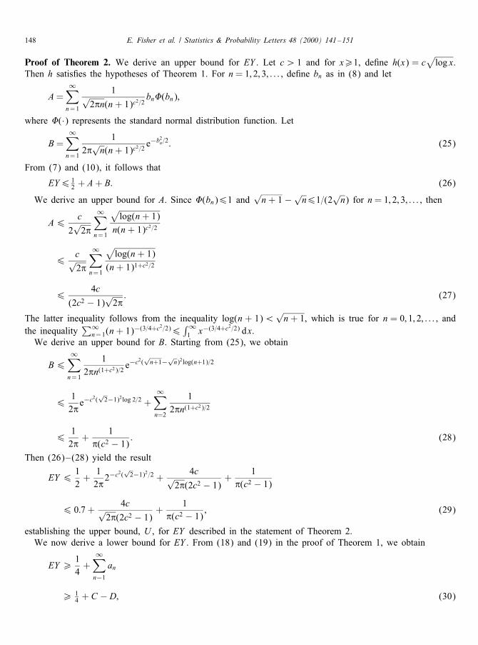
Proof of Theorem 2. We derive an upper bound for EY . Let c¿ 1 and for x¿1, de�ne h(x) = c√log x.

Then h satis�es the hypotheses of Theorem 1. For n= 1; 2; 3; : : : ; de�ne bn as in (8) and let

A=∞∑n=1

1√2�n(n+ 1)c2=2

bn�(bn);

where �(·) represents the standard normal distribution function. Let

B=∞∑n=1

12�

√n(n+ 1)c2=2

e−b2n=2: (25)

From (7) and (10), it follows that

EY6 12 + A+ B: (26)

We derive an upper bound for A. Since �(bn)61 and√n+ 1−√

n61=(2√n) for n= 1; 2; 3; : : : ; then

A6c

2√2�

∞∑n=1

√log(n+ 1)n(n+ 1)c2=2

6c√2�

∞∑n=1

√log(n+ 1)

(n+ 1)1+c2=2

64c

(2c2 − 1)√2� : (27)

The latter inequality follows from the inequality log(n + 1)¡√n+ 1, which is true for n = 0; 1; 2; : : : ; and

the inequality∑∞

n=1(n+ 1)−(3=4+c2=2)6

∫∞1 x−(3=4+c

2=2) dx.We derive an upper bound for B. Starting from (25), we obtain

B6∞∑n=1

12�n(1+c2)=2

e−c2(√n+1−√

n)2log(n+1)=2

612�e

−c2(√2−1)2log 2=2 +∞∑n=2

12�n(1+c2)=2

612� +

1�(c2 − 1) : (28)

Then (26)–(28) yield the result

EY 612+12�2

−c2(√2−1)2=2 +4c√

2�(2c2 − 1) +1

�(c2 − 1)

6 0:7 +4c√

2�(2c2 − 1) +1

�(c2 − 1) ; (29)

establishing the upper bound, U , for EY described in the statement of Theorem 2.We now derive a lower bound for EY . From (18) and (19) in the proof of Theorem 1, we obtain

EY ¿14+

∞∑n−1

an

¿ 14 + C − D; (30)


where

C =∞∑n=1

√n

2�(n+ 1)1+c2=2exp

[−c

2

2((√n+ 1−√

n)√log(n+ 1))2

]

and

D =∞∑n=1

c√n√

2�(n+ 1)1+c2=2(√n+ 1−√

n)√log(n+ 1)(1− �(bn)): (31)

The standard inequality exp(−x)¿− x, valid for all x¿0, yieldsC¿C1 − C2; (32)

where

C1 =∞∑n=1

√n

2�(n+ 1)1+c2=2

and

C2 =∞∑n=1

c2√n

4�(n+ 1)1+c2=2(√n+ 1−√

n)2 log(n+ 1):

We apply the inequality√n+ 1−√

n61=(2√n), valid for n¿1, to obtain

C1 =∞∑n=1

12�

( √n+ 1

(n+ 1)1+c2=2− (

√n+ 1−√

n)(n+ 1)1+c2=2

)

¿∞∑n=1

12� (n+ 1)

−(1+c2)=2 −∞∑n=1

14�n

−(3+c2)=2:

Since∞∑n=1

12� (n+ 1)

−(1+c2)=2¿12�

∫ ∞

1(x + 1)−(1+c

2)=2 dx

=1

�(c2 − 1)2(1−c2)=2

and∞∑n=1

14�n

−(3+c2)=2614� +

14�

∫ ∞

1x−(3+c

2)=2 dx

=14� +

12�(c2 + 1) ;

then

C1¿1

�(c2 − 1)2(1−c2)=2 − 1

4� − 12�(c2 + 1) : (33)


We consider C2. The inequality 06√n+ 1−√

n61=(2√n) holds for n¿1. Hence,

C26116�

∞∑n=1

c2 log(n+ 1)√n(n+ 1)1+c2=2

=c2 log(2)16�21+c2=2

+116�

∞∑n=2

c2 log(n+ 1)√n(n+ 1)1+c2=2

:

We apply the inequality log(n+ 1)6√2n(n+ 1)−1=4 (for n¿2) to the latter sum and obtain

C26c2 log(2)16�21+c2=2

+

√2c2

16�

∞∑n=3

n−5=4−c2=2

6c2 log(2)16�21+c2=2

+

√2c2

16�

∫ ∞

2x−5=4−c

2=2 dx

=c2 log(2)16�21+c2=2

+21=4c2

4�(1 + 2c2)2−c2=2: (34)

Consider D as de�ned by (31). Applying the just employed upper bound for√n+ 1 − √

n, the fact1−�(bn)6 1

2 for n= 1; 2; 3; : : : ; and the inequality log(n+ 1)6√n+ 1 which holds for n= 1; 2; 3; : : : , leads

to the result

D6∞∑n=1

c

4√2�(n+ 1)1+c2=2

√log(n+ 1)

6∞∑n=1

c

4√2�(n+ 1)−(3=4+c

2=2)

6c

4√2�

∫ ∞

1x−(3=4+c

2=2) ds

=c√

2�(2c2 − 1) : (35)

Combining the results (30), (32)–(35), and noting that for c¿ 1, 14 − 1=(4�)− 1=(2�(c2 + 1))¿ 0 yields

EY ¿

√2

�(c2 − 1)2−c2=2 − c2 log 2

32� 2−c2=2 − c221=4

4�(1 + 2c2)2−c2=2 − c√

2�(2c2 − 1)

¿

√2

�(c2 − 1)2−c2=2 − 1√

2�− c22−c2=2

[log 232� +

21=4

4�(1 + 2c2)

]

¿

√2

�(c2 − 1)2−c2=2 − 1√

2�− 2(e)(log 2)

[log 232� +

21=4

12�

]

¿

√2

�(c2 − 1)2−c2=2 − 0:5:

The latter inequality establishes the lower bound, L, for EY described in the statement of Theorem 2.This, with (29), establishes the conclusion of Theorem 2.


References

Feller, W., 1968. An Introduction to Probability Theory and its Applications, 3rd Edition, Vol. 1. Wiley, New York.Klebaner, F.C., 1990. Expected number of excursions above curved boundarie by a random walk. Bull. Austral. Math. Soc. 41, 207–213.Lan, K.K., Lai, T.L., 1976. On the last time and the number of boundary crossings related to the strong law of large numbers.Z. Wahrscheinlichkeitsth 34, 59–71.

Slivka, J., 1969. On the law of the iterated logarithm. Proc. Natn. Acad. Sci. USA 63, 289–291.Stout, W.F., 1974. Almost Sure Convergence. Academic Press, New York.Stratton, H.H., 1972, Moments of oscillations and related sums. Ann. Math. Statist. 1012–1016.

Documents

Excursions of a normal random walk above a boundary