Exchange Rate YuYuan Liu Han Yu Yang Dennis Yue Jessica Chen Jo-Yu Mao

Exchange Rate

YuYuan Liu Han Yu Yang Dennis Yue Jessica Chen Jo-Yu Mao

Introduction

In finance, the foreign-exchange rate between two currencies specifies how much one currency is worth in terms of the other.

It has a major impact on a country’s ability on importing and exporting, inflations, foreign investment, and foreign debts.

Introduction U.S. urges China to open

currency exchange in order to balance import and export proportions.

Introduction

Sets of data Trade-Weighted Index Japan United Kingdom Canada

Dates: 1973:01 to 2006:03

Trade-Weighted Index

Regression on Time For TWI Dependent Variable: TWI Method: Least Squares Date: 06/06/06 Time: 15:28 Sample(adjusted): 1973:01 2004:04 Included observations: 376 after adjusting endpoints

Variable Coefficient Std. Error t-Statistic Prob.

TIME -0.035760 0.005498 -6.504630 0.0000 C 107.7983 1.306926 82.48235 0.0000

R-squared 0.101631 Mean dependent var 100.2351 Adjusted R-squared 0.099229 S.D. dependent var 12.19151 S.E. of regression 11.57083 Akaike info criterion 7.740157 Sum squared resid 50072.67 Schwarz criterion 7.761059 Log likelihood -1453.149 F-statistic 42.31022 Durbin-Watson stat 0.022781 Prob(F-statistic) 0.000000

-20

0

20

40

60

60

80

100

120

140

160

75 80 85 90 95 00

Residual Actual Fitted

TWI Series

60

80

100

120

140

160

75 80 85 90 95 00 05

TWI

0

10

20

30

40

50

80 90 100 110 120 130 140

Series: TWISample 1973:01 2006:03Observations 399

Mean 99.32301Median 97.11000Maximum 143.9100Minimum 80.11000Std. Dev. 12.40890Skewness 1.112975Kurtosis 4.258971

Jarque-Bera 108.7251Probability 0.000000

Correlogram and Unit root test for TWI

Date: 06/06/06 Time: 14:17 Sample: 1973:01 2007:12 Included observations: 399

Autocorrelation Partial Correlation AC PAC Q-Stat Prob

.|******** .|******** 1 0.988 0.988 392.49 0.000 .|*******| **|. | 2 0.971 -0.236 772.27 0.000 .|*******| .|. | 3 0.953 0.043 1139.5 0.000 .|*******| .|. | 4 0.935 -0.055 1493.7 0.000 .|*******| .|. | 5 0.917 -0.004 1835.0 0.000 .|*******| .|. | 6 0.898 -0.001 2163.6 0.000 .|*******| .|. | 7 0.881 0.013 2480.1 0.000 .|*******| .|. | 8 0.862 -0.055 2784.4 0.000 .|****** | *|. | 9 0.842 -0.074 3075.1 0.000 .|****** | .|. | 10 0.820 -0.054 3351.6 0.000 .|****** | *|. | 11 0.795 -0.107 3612.4 0.000 .|****** | .|. | 12 0.769 -0.057 3856.6 0.000 .|****** | *|. | 13 0.740 -0.060 4083.8 0.000 .|***** | .|. | 14 0.712 0.016 4294.7 0.000 .|***** | .|. | 15 0.684 -0.054 4489.5 0.000 .|***** | .|. | 16 0.655 -0.010 4668.8 0.000 .|***** | .|. | 17 0.627 0.022 4833.7 0.000 .|***** | .|. | 18 0.602 0.060 4985.6 0.000 .|**** | .|. | 19 0.575 -0.053 5125.0 0.000 .|**** | .|. | 20 0.549 0.011 5252.2 0.000 .|**** | .|. | 21 0.523 0.002 5367.9 0.000 .|**** | .|. | 22 0.496 -0.014 5472.4 0.000 .|**** | .|. | 23 0.470 -0.003 5566.4 0.000 .|*** | *|. | 24 0.442 -0.075 5649.8 0.000 .|*** | .|. | 25 0.415 0.031 5723.5 0.000 .|*** | .|. | 26 0.389 -0.015 5788.3 0.000 .|*** | .|. | 27 0.363 0.024 5845.1 0.000 .|*** | *|. | 28 0.338 -0.063 5894.4 0.000 .|** | .|. | 29 0.314 0.026 5937.0 0.000 .|** | .|. | 30 0.290 -0.025 5973.5 0.000 .|** | .|. | 31 0.267 0.026 6004.5 0.000 .|** | .|. | 32 0.244 -0.057 6030.4 0.000 .|** | .|. | 33 0.221 0.003 6051.6 0.000 .|** | .|. | 34 0.198 0.004 6068.8 0.000 .|* | .|. | 35 0.176 -0.010 6082.4 0.000 .|* | .|. | 36 0.154 -0.019 6092.8 0.000

ADF Test Statistic -1.241982 1% Critical Value* -3.4489 5% Critical Value -2.8690 10% Critical Value -2.5707

*MacKinnon critical values for rejection of hypothesis of a unit root.

Augmented Dickey-Fuller Test Equation Dependent Variable: D(TWI) Method: Least Squares Date: 06/06/06 Time: 14:29 Sample(adjusted): 1973:02 2006:03 Included observations: 398 after adjusting endpoints


TWI(-1) -0.008656 0.006969 -1.241982 0.2150 C 0.802162 0.697805 1.149551 0.2510

R-squared 0.003880 Mean dependent var -0.057839 Adjusted R-squared 0.001365 S.D. dependent var 1.723604 S.E. of regression 1.722427 Akaike info criterion 3.930358 Sum squared resid 1174.835 Schwarz criterion 3.950391 Log likelihood -780.1413 F-statistic 1.542518 Durbin-Watson stat 1.345903 Prob(F-statistic) 0.214978

First Differencing

-8

-6

-4

-2

0

2

4

6

75 80 85 90 95 00 05

DTWI

0

10

20

30

40

50

60

-6 -4 -2 0 2 4

Series: DTWISample 1973:02 2006:03Observations 398

Mean -0.057839Median 0.065000Maximum 5.460000Minimum -6.900000Std. Dev. 1.723604Skewness -0.310463Kurtosis 3.721134


Correlogram and Unit root test for DTWI



.|** | .|** | 1 0.316 0.316 39.949 0.000 .|. | *|. | 2 0.021 -0.087 40.132 0.000 .|. | .|* | 3 0.049 0.078 41.115 0.000 .|. | .|. | 4 0.030 -0.011 41.478 0.000 .|. | .|. | 5 -0.014 -0.020 41.562 0.000 .|. | .|. | 6 -0.032 -0.023 41.971 0.000 .|. | .|. | 7 0.033 0.054 42.423 0.000 .|* | .|* | 8 0.114 0.095 47.714 0.000 .|* | .|. | 9 0.078 0.019 50.205 0.000 .|* | .|* | 10 0.095 0.079 53.873 0.000 .|* | .|. | 11 0.081 0.020 56.549 0.000 .|. | .|. | 12 0.034 0.001 57.015 0.000 .|. | .|. | 13 0.016 0.009 57.128 0.000 .|. | .|. | 14 0.032 0.029 57.544 0.000 .|. | .|. | 15 0.009 -0.014 57.578 0.000 .|. | .|. | 16 -0.033 -0.040 58.032 0.000 *|. | *|. | 17 -0.071 -0.067 60.163 0.000 .|. | .|* | 18 0.036 0.067 60.714 0.000 .|. | .|. | 19 0.003 -0.055 60.718 0.000 .|. | .|. | 20 -0.021 -0.002 60.895 0.000 .|. | .|. | 21 0.024 0.020 61.144 0.000 .|. | .|. | 22 0.028 -0.003 61.466 0.000 .|. | .|. | 23 0.055 0.053 62.746 0.000 .|. | *|. | 24 -0.036 -0.074 63.303 0.000 .|. | .|. | 25 -0.054 -0.006 64.555 0.000 *|. | *|. | 26 -0.060 -0.059 66.070 0.000 .|. | .|* | 27 0.013 0.077 66.145 0.000 .|. | .|. | 28 -0.020 -0.051 66.320 0.000 .|. | .|. | 29 -0.030 0.000 66.702 0.000 .|. | .|. | 30 -0.021 -0.022 66.889 0.000 .|. | .|. | 31 0.024 0.032 67.140 0.000 .|. | .|. | 32 -0.027 -0.054 67.461 0.000 .|. | .|. | 33 -0.052 -0.022 68.632 0.000 .|. | .|. | 34 -0.008 0.024 68.658 0.000 .|. | .|. | 35 0.037 0.044 69.248 0.000 *|. | *|. | 36 -0.063 -0.093 70.973 0.000



Augmented Dickey-Fuller Test Equation Dependent Variable: D(DTWI) Method: Least Squares Date: 06/06/06 Time: 15:06 Sample(adjusted): 1973:03 2006:03 Included observations: 397 after adjusting endpoints


DTWI(-1) -0.684369 0.047309 -14.46604 0.0000 C -0.028539 0.081587 -0.349796 0.7267


Fitting ARMA Model Dependent Variable: dtwi Method: Least Squares Date: 05/27/06 Time: 15:08 Sample(adjusted): 1973:02 2006:04 Included observations: 399 after adjusting endpoints Convergence achieved after 4 iterations Backcast: 1973:01


C -0.062670 0.110268 -0.568337 0.5701 MA(1) 0.356248 0.046850 7.604032 0.0000


Inverted MA Roots -.36

-10

-5

0

5

10

-10

-5

0

5

10

75 80 85 90 95 00 05


0

10

20

30

40

50

60

-6 -4 -2 0 2 4 6

Series: ResidualsSample 1973:02 2006:03Observations 398

Mean 0.001692Median 0.069711Maximum 6.380749Minimum -7.331638Std. Dev. 1.624205Skewness -0.290877Kurtosis 4.661199


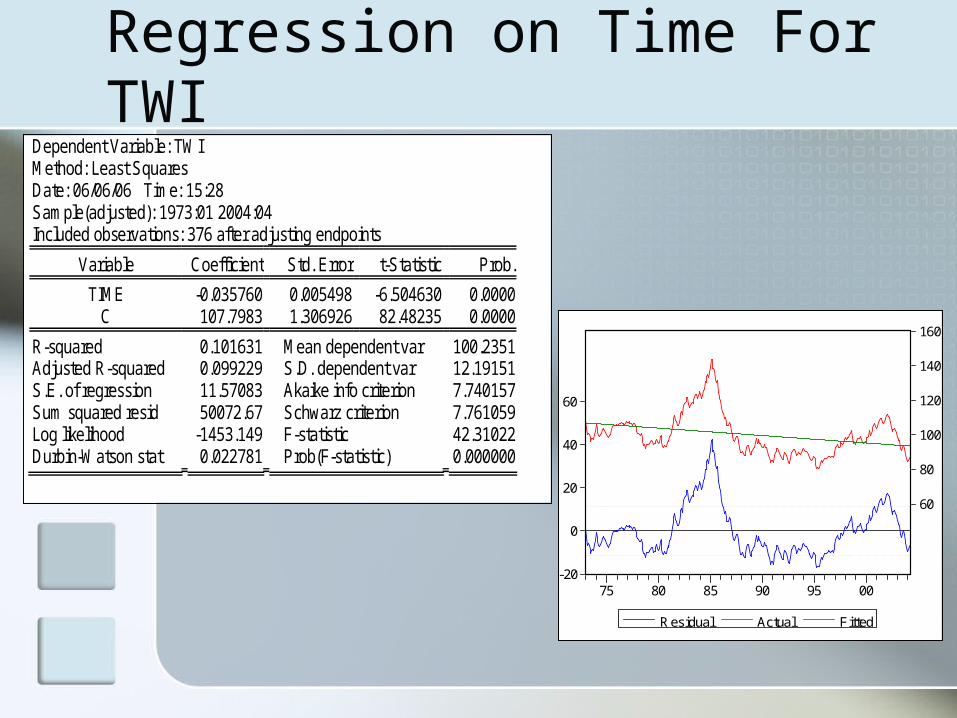
Serial Correlation Test and Correlogram for MAone model Residuals

Breusch-Godfrey Serial Correlation LM Test:

F-statistic 0.063872 Probability 0.800609 Obs*R-squared 0.063914 Probability 0.800413

Test Equation: Dependent Variable: RESID Method: Least Squares Date: 06/06/06 Time: 15:53


C 0.000170 0.110579 0.001535 0.9988 MA(1) 0.030863 0.130834 0.235895 0.8136

RESID(-1) -0.035421 0.140153 -0.252730 0.8006

R-squared 0.000161 Mean dependent var 0.001692 Adjusted R-squared -0.004902 S.D. dependent var 1.624205 S.E. of regression 1.628181 Akaike info criterion 3.820313 Sum squared resid 1047.135 Schwarz criterion 3.850362 Log likelihood -757.2423 F-statistic 0.031721 Durbin-Watson stat 1.984334 Prob(F-statistic) 0.968779


Q-statistic probabilities

adjusted for 1 ARMA term(s)


.|. | .|. | 1 -0.005 -0.005 0.0084 .|. | .|. | 2 0.010 0.010 0.0521 0.819 .|. | .|. | 3 0.039 0.040 0.6801 0.712 .|. | .|. | 4 0.021 0.021 0.8548 0.836 .|. | .|. | 5 -0.012 -0.013 0.9129 0.923 .|. | .|. | 6 -0.031 -0.033 1.3041 0.935 .|. | .|. | 7 0.011 0.009 1.3515 0.969 .|* | .|* | 8 0.103 0.105 5.6648 0.579 .|. | .|. | 9 0.024 0.029 5.9073 0.658 .|* | .|* | 10 0.070 0.069 7.9048 0.544 .|. | .|. | 11 0.055 0.047 9.1494 0.518 .|. | .|. | 12 0.015 0.008 9.2411 0.600 .|. | .|. | 13 0.002 -0.002 9.2421 0.682 .|. | .|. | 14 0.031 0.032 9.6303 0.724 .|. | .|. | 15 0.000 0.000 9.6303 0.789 .|. | .|. | 16 -0.004 -0.010 9.6361 0.842 *|. | *|. | 17 -0.091 -0.099 13.117 0.664 .|* | .|. | 18 0.069 0.052 15.103 0.588 .|. | .|. | 19 -0.009 -0.020 15.139 0.652 .|. | .|. | 20 -0.029 -0.031 15.493 0.691 .|. | .|. | 21 0.036 0.027 16.028 0.715 .|. | .|. | 22 -0.007 -0.022 16.050 0.767 .|* | .|* | 23 0.074 0.071 18.373 0.684 .|. | .|. | 24 -0.055 -0.055 19.664 0.662 .|. | .|. | 25 -0.016 -0.003 19.768 0.710 *|. | *|. | 26 -0.068 -0.083 21.767 0.649 .|. | .|. | 27 0.045 0.064 22.632 0.654 .|. | .|. | 28 -0.031 -0.021 23.045 0.683 .|. | .|. | 29 -0.009 -0.007 23.084 0.729 .|. | .|. | 30 -0.030 -0.034 23.483 0.754 .|. | .|. | 31 0.043 0.035 24.289 0.759 .|. | .|. | 32 -0.029 -0.029 24.644 0.783 .|. | .|. | 33 -0.039 -0.039 25.315 0.793 .|. | .|. | 34 -0.012 -0.006 25.380 0.826 .|. | .|* | 35 0.055 0.066 26.688 0.810 .|. | .|. | 36 -0.043 -0.033 27.511 0.812

Diagnosis for ARMA model: Residuals Squared Series

0

10

20

30

40

50

60

75 80 85 90 95 00 05

TWI_RESIDSQ

0

50

100

150

200

250

300

0 10 20 30 40 50

Series: TWI_RESIDSQSample 1973:02 2006:03Observations 398

Mean 2.631417Median 0.815092Maximum 53.75291Minimum 7.35E-07Std. Dev. 5.040521Skewness 4.973275Kurtosis 39.14255


Conditional Heteroscedasticity test: Correlogram of residuals squared and ARCH-test



.|. | .|. | 1 -0.027 -0.027 0.2981 0.585 .|. | .|. | 2 0.062 0.061 1.8314 0.400 .|* | .|* | 3 0.100 0.104 5.8561 0.119 .|* | .|* | 4 0.113 0.116 10.980 0.027 .|* | .|* | 5 0.094 0.093 14.562 0.012 .|* | .|* | 6 0.130 0.119 21.396 0.002 .|* | .|* | 7 0.084 0.068 24.259 0.001 .|* | .|. | 8 0.066 0.036 26.056 0.001 .|* | .|* | 9 0.125 0.087 32.494 0.000 .|* | .|. | 10 0.084 0.050 35.393 0.000 .|. | .|. | 11 0.038 -0.005 35.994 0.000 .|. | .|. | 12 0.056 -0.001 37.265 0.000 .|. | .|. | 13 0.064 0.009 38.934 0.000 .|. | .|. | 14 0.017 -0.032 39.051 0.000 .|* | .|* | 15 0.126 0.078 45.682 0.000 .|. | .|. | 16 0.013 -0.019 45.749 0.000 .|. | .|. | 17 0.048 0.010 46.694 0.000 .|. | .|. | 18 0.041 0.002 47.383 0.000 .|. | .|. | 19 0.020 -0.023 47.545 0.000 .|. | .|. | 20 0.047 0.016 48.478 0.000 .|* | .|. | 21 0.074 0.045 50.805 0.000 .|. | .|. | 22 -0.008 -0.031 50.834 0.000 .|. | .|. | 23 0.018 -0.011 50.975 0.001 .|. | *|. | 24 -0.022 -0.065 51.189 0.001 .|* | .|* | 25 0.153 0.129 61.229 0.000 .|. | .|. | 26 -0.007 -0.004 61.247 0.000 .|. | .|. | 27 0.005 -0.018 61.259 0.000 .|. | .|. | 28 0.057 0.036 62.655 0.000 .|. | .|. | 29 -0.007 -0.026 62.677 0.000 .|. | .|. | 30 0.020 -0.017 62.847 0.000 .|. | .|. | 31 0.008 -0.019 62.875 0.001 .|. | .|. | 32 0.041 0.023 63.617 0.001 .|. | .|. | 33 -0.005 -0.010 63.627 0.001 .|* | .|* | 34 0.114 0.093 69.288 0.000 .|. | .|. | 35 0.004 -0.002 69.296 0.000 .|. | .|. | 36 0.039 0.027 69.952 0.001

ARCH Test:


Test Equation: Dependent Variable: RESID^2 Method: Least Squares Date: 06/06/06 Time: 14:05 Sample(adjusted): 1973:03 2006:03 Included observations: 397 after adjusting endpoints


C 2.669503 0.283571 9.413872 0.0000 RESID^2(-1) -0.027274 0.049858 -0.547029 0.5847


Forecast of TWIobs TWI TWIF DTWI DTWIF UPPERTWI LOWERTWI

2006:03 85.17000 85.17000 -0.050000 -0.050000 NA NA 2006:04 NA 84.96498 NA -0.205016 88.21750 81.71247 2006:05 NA 84.90542 NA -0.059565 88.35742 81.45342 2006:06 NA 84.84585 NA -0.059565 88.29785 81.39385 2006:07 NA 84.78629 NA -0.059565 88.23829 81.33429 2006:08 NA 84.72672 NA -0.059565 88.17873 81.27472 2006:09 NA 84.66716 NA -0.059565 88.11916 81.21516 2006:10 NA 84.60759 NA -0.059565 88.05960 81.15559 2006:11 NA 84.54803 NA -0.059565 88.00003 81.09603 2006:12 NA 84.48847 NA -0.059565 87.94047 81.03646 2007:01 NA 84.42890 NA -0.059565 87.88090 80.97690 2007:02 NA 84.36934 NA -0.059565 87.82134 80.91733 2007:03 NA 84.30977 NA -0.059565 87.76177 80.85777 2007:04 NA 84.25021 NA -0.059565 87.70221 80.79820 2007:05 NA 84.19064 NA -0.059565 87.64264 80.73864 2007:06 NA 84.13108 NA -0.059565 87.58308 80.67908 2007:07 NA 84.07151 NA -0.059565 87.52351 80.61951 2007:08 NA 84.01195 NA -0.059565 87.46395 80.55995 2007:09 NA 83.95238 NA -0.059565 87.40438 80.50038 2007:10 NA 83.89282 NA -0.059565 87.34482 80.44082 2007:11 NA 83.83325 NA -0.059565 87.28525 80.38125 2007:12 NA 83.77369 NA -0.059565 87.22569 80.32169

Forecast of TWI

-4

-2

0

2

4

06:04 06:07 06:10 07:01 07:04 07:07 07:10

DT WIF ± 2 S.E.

60

80

100

120

140

160

75 80 85 90 95 00 05

TWITWIF

UPPERTWILOWERTWI

Japan

Regression on Time For Japan

Dependent Variable: JAPAN Method: Least Squares Date: 06/06/06 Time: 17:50 Sample(adjusted): 1973:01 2004:04 Included observations: 376 after adjusting endpoints


TIME -0.553826 0.014282 -38.77912 0.0000 C 293.3687 3.395091 86.40967 0.0000


-100

-50

0

50

100

50

100

150

200

250

300

350

75 80 85 90 95 00


Japan Series

50

100

150

200

250

300

350

75 80 85 90 95 00 05

JAPAN

0

10

20

30

40

50

60

80 100 120 140 160 180 200 220 240 260 280 300

Series: JAPANSample 1973:01 2006:03Observations 399



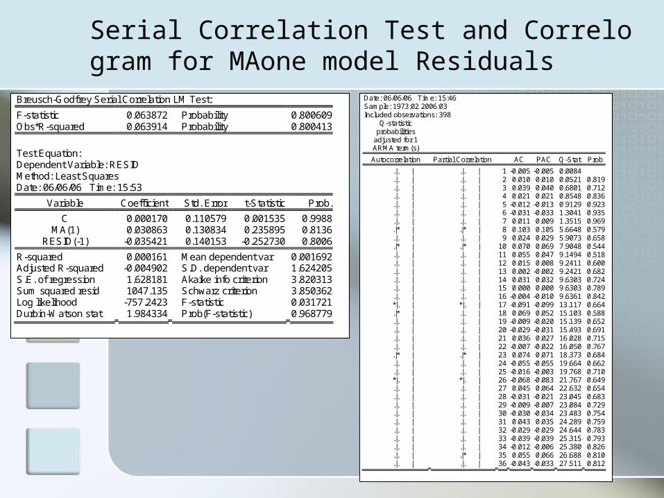
Correlogram and Unit root test for Japan



.|******** .|******** 1 0.993 0.993 396.64 0.000 .|******** .|. | 2 0.986 -0.056 788.37 0.000 .|******** .|. | 3 0.978 -0.028 1174.9 0.000 .|*******| .|. | 4 0.970 -0.027 1556.1 0.000 .|*******| .|. | 5 0.962 -0.028 1931.5 0.000 .|*******| .|. | 6 0.953 -0.011 2301.2 0.000 .|*******| .|. | 7 0.944 0.005 2665.2 0.000 .|*******| .|. | 8 0.936 -0.021 3023.5 0.000 .|*******| .|. | 9 0.926 -0.035 3375.6 0.000 .|*******| *|. | 10 0.916 -0.075 3721.0 0.000 .|*******| .|. | 11 0.906 -0.006 4059.5 0.000 .|*******| *|. | 12 0.894 -0.126 4389.9 0.000 .|*******| .|. | 13 0.882 0.018 4712.5 0.000 .|*******| .|* | 14 0.871 0.067 5027.9 0.000 .|*******| .|. | 15 0.861 0.018 5336.4 0.000 .|*******| .|. | 16 0.850 -0.015 5638.1 0.000 .|****** | .|. | 17 0.839 0.012 5933.0 0.000 .|****** | .|. | 18 0.829 -0.002 6221.4 0.000 .|****** | .|. | 19 0.818 -0.032 6503.1 0.000 .|****** | .|. | 20 0.807 0.038 6778.3 0.000 .|****** | .|. | 21 0.797 0.037 7047.5 0.000 .|****** | .|. | 22 0.788 0.015 7310.9 0.000 .|****** | .|. | 23 0.778 -0.015 7568.5 0.000 .|****** | *|. | 24 0.768 -0.062 7820.0 0.000 .|****** | .|. | 25 0.758 0.016 8065.7 0.000 .|****** | .|. | 26 0.749 0.027 8306.1 0.000 .|****** | .|. | 27 0.739 -0.038 8540.8 0.000 .|****** | .|. | 28 0.729 -0.014 8769.9 0.000 .|****** | .|. | 29 0.719 -0.033 8993.2 0.000 .|***** | .|. | 30 0.708 -0.031 9210.5 0.000 .|***** | .|. | 31 0.697 -0.054 9421.7 0.000 .|***** | .|. | 32 0.685 -0.036 9626.6 0.000 .|***** | .|. | 33 0.674 0.030 9825.4 0.000 .|***** | .|. | 34 0.663 0.016 10018. 0.000 .|***** | .|. | 35 0.652 -0.042 10205. 0.000 .|***** | .|. | 36 0.640 -0.033 10386. 0.000



Augmented Dickey-Fuller Test Equation Dependent Variable: D(JAPAN) Method: Least Squares Date: 06/06/06 Time: 17:52 Sample(adjusted): 1973:01 2006:03 Included observations: 399 after adjusting endpoints


JAPAN(-1) -0.006579 0.003752 -1.753333 0.0803 C 0.674664 0.696158 0.969124 0.3331


First Differencing

-8

-6

-4

-2

0

2

4

6

75 80 85 90 95 00 05

DTWI

0

10

20

30

40

50

60

-6 -4 -2 0 2 4

Series: DTWISample 1973:02 2006:03Observations 398

Mean -0.057839Median 0.065000Maximum 5.460000Minimum -6.900000Std. Dev. 1.723604Skewness -0.310463Kurtosis 3.721134


Correlogram and Unit root test for DJapan



.|** | .|** | 1 0.307 0.307 37.869 0.000 .|. | *|. | 2 0.026 -0.076 38.131 0.000 .|. | .|* | 3 0.053 0.076 39.265 0.000 .|* | .|. | 4 0.079 0.045 41.791 0.000 .|. | .|. | 5 0.020 -0.019 41.946 0.000 .|. | .|. | 6 -0.052 -0.055 43.037 0.000 .|. | .|. | 7 0.013 0.047 43.109 0.000 .|. | .|. | 8 0.061 0.038 44.604 0.000 .|. | .|. | 9 0.051 0.029 45.682 0.000 .|. | .|. | 10 -0.023 -0.044 45.895 0.000 .|* | .|* | 11 0.092 0.123 49.365 0.000 .|. | .|. | 12 0.055 -0.032 50.610 0.000 *|. | *|. | 13 -0.081 -0.095 53.331 0.000 .|. | .|. | 14 -0.022 0.044 53.532 0.000 .|. | .|. | 15 -0.009 -0.035 53.570 0.000 *|. | *|. | 16 -0.091 -0.101 57.054 0.000 *|. | .|. | 17 -0.112 -0.036 62.282 0.000 .|. | .|. | 18 -0.033 0.017 62.745 0.000 .|. | *|. | 19 -0.048 -0.069 63.697 0.000 *|. | .|. | 20 -0.084 -0.053 66.669 0.000 *|. | .|. | 21 -0.095 -0.031 70.445 0.000 .|. | .|. | 22 0.012 0.053 70.506 0.000 .|* | .|* | 23 0.125 0.100 77.121 0.000 .|. | *|. | 24 -0.038 -0.079 77.742 0.000 *|. | .|. | 25 -0.059 0.007 79.249 0.000 .|. | .|. | 26 0.027 0.025 79.563 0.000 .|. | .|. | 27 0.027 0.006 79.868 0.000 .|. | .|. | 28 0.022 0.061 80.069 0.000 .|. | .|. | 29 0.034 0.029 80.555 0.000 .|* | .|. | 30 0.073 0.043 82.866 0.000 .|* | .|. | 31 0.068 0.030 84.886 0.000 *|. | *|. | 32 -0.075 -0.133 87.351 0.000 .|. | .|. | 33 -0.046 0.014 88.272 0.000 .|* | .|. | 34 0.069 0.036 90.344 0.000 .|. | .|. | 35 0.057 0.014 91.751 0.000 .|. | .|. | 36 -0.046 -0.047 92.680 0.000



Augmented Dickey-Fuller Test Equation Dependent Variable: D(DJAPAN) Method: Least Squares Date: 06/06/06 Time: 17:55 Sample(adjusted): 1973:03 2006:03 Included observations: 397 after adjusting endpoints


DJAPAN(-1) -0.692698 0.047161 -14.68789 0.0000 C -0.240079 0.233117 -1.029866 0.3037


Fitting ARMA ModelDependent Variable: DJAPAN Method: Least Squares Date: 06/06/06 Time: 17:19 Sample(adjusted): 1973:02 2006:03 Included observations: 398 after adjusting endpoints Convergence achieved after 6 iterations Backcast: 1971:03 1973:01


C -0.399414 0.350316 -1.140155 0.2549 MA(1) 0.346135 0.045238 7.651430 0.0000

MA(23) 0.185975 0.045967 4.045788 0.0001


Inverted MA Roots .91+.13i .91 -.13i .84+.37i .84 -.37i .71+.59i .71 -.59i .52 -.76i .52+.76i .30 -.87i .30+.87i .05+.92i .05 -.92i -.20+.91i -.20 -.91i -.44+.82i -.44 -.82i -.65+.68i -.65 -.68i -.81+.48i -.81 -.48i -.91+.25i -.91 -.25i -.95

Diagnosis of ARMA model:residuals graph and histogram

-30

-20

-10

0

10

20

-30

-20

-10

0

10

20

75 80 85 90 95 00 05


0

20

40

60

80

100

120

-20 -10 0 10 20




Diagnosis of ARMA model: Correlogram-Qstat of ARMA model & Serial correlation testDate: 06/06/06 Time: 17:58 Sample: 1973:02 2006:03 Included observations: 398




.|. | .|. | 1 0.003 0.003 0.0033 .|. | .|. | 2 0.036 0.036 0.5301 .|. | .|. | 3 0.031 0.031 0.9186 0.338 .|* | .|* | 4 0.069 0.068 2.8575 0.240 .|. | .|. | 5 0.023 0.021 3.0683 0.381 *|. | *|. | 6 -0.058 -0.064 4.4292 0.351 .|. | .|. | 7 0.029 0.024 4.7748 0.444 .|. | .|. | 8 0.015 0.013 4.8674 0.561 .|* | .|* | 9 0.073 0.072 7.0208 0.427 .|. | .|. | 10 -0.038 -0.034 7.6271 0.471 .|* | .|. | 11 0.071 0.065 9.7135 0.374 .|. | .|. | 12 0.043 0.034 10.467 0.400 *|. | *|. | 13 -0.094 -0.106 14.152 0.225 .|. | .|. | 14 0.005 0.002 14.162 0.291 .|. | .|. | 15 0.021 0.028 14.352 0.350 *|. | *|. | 16 -0.072 -0.085 16.519 0.283 *|. | .|. | 17 -0.060 -0.043 18.014 0.262 .|. | .|. | 18 -0.025 -0.018 18.266 0.309 .|. | .|. | 19 -0.033 -0.041 18.731 0.344 *|. | *|. | 20 -0.063 -0.060 20.409 0.310 *|. | .|. | 21 -0.060 -0.042 21.921 0.288 .|. | .|. | 22 -0.012 0.002 21.982 0.341 .|. | .|. | 23 -0.029 -0.036 22.333 0.381 .|. | .|. | 24 0.009 0.033 22.368 0.438 *|. | .|. | 25 -0.060 -0.030 23.916 0.408 .|. | .|. | 26 0.047 0.035 24.872 0.413 .|. | .|. | 27 0.002 0.016 24.873 0.469 .|. | .|. | 28 0.021 0.046 25.055 0.516 .|. | .|. | 29 0.023 0.024 25.281 0.559 .|. | .|. | 30 0.033 0.034 25.738 0.587 .|* | .|* | 31 0.082 0.086 28.651 0.483 *|. | *|. | 32 -0.094 -0.093 32.470 0.346 .|. | *|. | 33 -0.033 -0.065 32.944 0.372 .|. | .|. | 34 0.052 0.060 34.145 0.365 .|. | .|. | 35 0.037 0.020 34.761 0.384 .|. | .|. | 36 -0.012 -0.018 34.819 0.429





C 0.005155 0.350919 0.014691 0.9883 MA(1) 0.104096 0.164247 0.633778 0.5266

MA(23) -0.006979 0.047571 -0.146713 0.8834 RESID(-1) -0.102524 0.173603 -0.590566 0.5552 RESID(-2) 0.072758 0.076570 0.950206 0.3426



0

100

200

300

400

500

600

75 80 85 90 95 00 05

JAPAN_RESIDSQ

0

100

200

300

400

0 50 100 150 200 250 300 350 400 450 500

Series: JAPAN_RESIDSQSample 1973:02 2006:03Observations 398

Mean 20.87996Median 6.665713Maximum 512.0115Minimum 6.83E-05Std. Dev. 47.67450Skewness 5.836261Kurtosis 46.41566


Conditional Heteroscedasticity test: Correlogram of residuals squared and ARCH-testDate: 06/06/06 Time: 18:00 Sample: 1973:02 2006:03 Included observations: 398




.|* | .|* | 1 0.106 0.106 4.4820 .|. | .|. | 2 0.055 0.045 5.7198 .|. | .|. | 3 0.050 0.040 6.7342 0.009 .|* | .|* | 4 0.104 0.093 11.066 0.004 .|. | .|. | 5 0.046 0.023 11.918 0.008 .|* | .|* | 6 0.150 0.136 21.038 0.000 .|* | .|* | 7 0.110 0.077 25.976 0.000 .|* | .|. | 8 0.066 0.030 27.757 0.000 .|. | .|. | 9 0.057 0.030 29.086 0.000 .|* | .|. | 10 0.097 0.059 32.982 0.000 .|. | .|. | 11 0.032 -0.009 33.396 0.000 .|. | .|. | 12 0.012 -0.028 33.453 0.000 .|. | .|. | 13 0.041 0.006 34.162 0.000 .|. | .|. | 14 -0.001 -0.041 34.162 0.001 .|. | .|. | 15 0.062 0.043 35.744 0.001 .|. | .|. | 16 0.041 0.006 36.460 0.001 .|. | .|. | 17 0.040 0.014 37.142 0.001 .|* | .|* | 18 0.101 0.096 41.447 0.000 .|. | .|. | 19 0.045 0.012 42.281 0.001 .|. | .|. | 20 0.001 -0.017 42.281 0.001 .|. | .|. | 21 0.037 0.021 42.850 0.001 .|. | .|. | 22 -0.006 -0.041 42.867 0.002 .|* | .|. | 23 0.067 0.051 44.753 0.002 .|. | .|. | 24 0.030 -0.008 45.126 0.003 .|* | .|* | 25 0.154 0.124 55.304 0.000 .|. | .|. | 26 0.013 -0.024 55.372 0.000 .|. | .|. | 27 0.002 -0.025 55.374 0.000 .|. | .|. | 28 0.008 -0.012 55.399 0.001 .|. | .|. | 29 -0.018 -0.056 55.533 0.001 .|. | .|. | 30 0.026 0.025 55.830 0.001 .|* | .|* | 31 0.155 0.120 66.244 0.000 .|. | .|. | 32 0.011 -0.029 66.294 0.000 .|. | .|. | 33 -0.004 -0.022 66.302 0.000 .|* | .|* | 34 0.146 0.143 75.685 0.000 .|. | .|. | 35 0.005 -0.052 75.696 0.000 .|. | .|. | 36 0.022 0.008 75.907 0.000

ARCH Test:




C 18.24618 2.564280 7.115518 0.0000 RESID^2(-1) 0.105781 0.049259 2.147444 0.0324


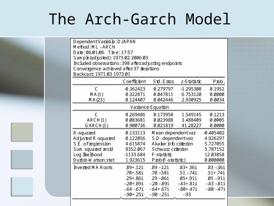
The Arch-Garch ModelDependent Variable: DJAPAN Method: ML - ARCH Date: 06/01/06 Time: 17:57 Sample(adjusted): 1973:02 2006:03 Included observations: 398 after adjusting endpoints Convergence achieved after 37 iterations Backcast: 1971:03 1973:01

Coefficient Std. Error z-Statistic Prob.

C -0.362423 0.279797 -1.295308 0.1952 MA(1) 0.322871 0.047811 6.753120 0.0000

MA(23) 0.124407 0.042446 2.930925 0.0034

Variance Equation

C 0.269486 0.173958 1.549145 0.1213 ARCH(1) 0.083681 0.023988 3.488409 0.0005

GARCH(1) 0.900736 0.021819 41.28227 0.0000


Inverted MA Roots .89+.12i .89 -.12i .83+.36i .83 -.36i .70+.58i .70 -.58i .51 -.74i .51+.74i .29+.86i .29 -.86i .05+.91i .05 -.91i -.20+.89i -.20 -.89i -.43+.81i -.43 -.81i -.64 -.67i -.64+.67i -.80+.47i -.80 -.47i -.90+.25i -.90 -.25i -.93

Diagnosis for ARCH model

0

10

20

30

40

50

60

-5 -4 -3 -2 -1 0 1 2 3

Series: Standardized ResidualsSample 1973:02 2006:03Observations 398







.|. | .|. | 1 -0.005 -0.005 0.0097 *|. | *|. | 2 -0.060 -0.060 1.4627 .|. | .|. | 3 0.011 0.010 1.5087 0.219 .|. | .|. | 4 0.040 0.037 2.1558 0.340 .|. | .|. | 5 -0.014 -0.012 2.2355 0.525 .|. | .|. | 6 0.048 0.053 3.1742 0.529 .|. | .|. | 7 0.021 0.019 3.3473 0.647 .|. | .|. | 8 -0.006 -0.002 3.3640 0.762 .|. | .|. | 9 -0.021 -0.019 3.5507 0.830 .|. | .|. | 10 0.002 -0.004 3.5518 0.895 .|. | .|. | 11 -0.040 -0.043 4.1948 0.898 .|. | .|. | 12 -0.012 -0.014 4.2578 0.935 .|. | .|. | 13 -0.007 -0.013 4.2796 0.961 *|. | *|. | 14 -0.070 -0.072 6.2912 0.901 .|. | .|. | 15 0.004 0.008 6.2989 0.935 .|. | .|. | 16 -0.005 -0.013 6.3106 0.958 .|. | .|. | 17 -0.012 -0.005 6.3664 0.973 .|. | .|. | 18 0.041 0.048 7.0557 0.972 .|. | .|. | 19 -0.004 -0.005 7.0612 0.983 .|. | .|. | 20 -0.036 -0.024 7.5985 0.984 .|. | .|. | 21 -0.003 -0.002 7.6018 0.990 *|. | *|. | 22 -0.059 -0.070 9.0700 0.982 .|. | .|. | 23 0.005 0.003 9.0824 0.989 .|. | .|. | 24 -0.023 -0.034 9.3132 0.992 .|* | .|* | 25 0.087 0.082 12.561 0.961 .|. | .|. | 26 -0.023 -0.019 12.787 0.970 *|. | .|. | 27 -0.063 -0.054 14.494 0.952 .|. | .|. | 28 -0.024 -0.026 14.741 0.962 .|. | *|. | 29 -0.055 -0.068 16.069 0.952 .|. | .|. | 30 -0.011 -0.008 16.118 0.964 .|. | .|. | 31 0.052 0.038 17.310 0.957 .|. | .|. | 32 -0.028 -0.024 17.654 0.964 .|. | .|. | 33 -0.030 -0.021 18.046 0.969 .|. | .|. | 34 0.064 0.064 19.850 0.954 .|. | .|. | 35 -0.002 -0.006 19.851 0.965 .|. | .|. | 36 0.005 0.012 19.860 0.974

Forecasting of Japanobs JAPAN JAPANF DJAPAN DJAPANF UPPERJAPAN LOWERJAPAN

2006:03 117.0700 117.0700 -0.210000 -0.210000 NA NA 2006:04 NA 116.2307 NA -0.839322 121.4682 110.9931 2006:05 NA 116.0185 NA -0.212216 121.5810 110.4559 2006:06 NA 115.7245 NA -0.293949 121.3504 110.0986 2006:07 NA 115.3265 NA -0.398022 121.0140 109.6390 2006:08 NA 114.9079 NA -0.418582 120.6554 109.1604 2006:09 NA 114.0809 NA -0.827038 119.8868 108.2749 2006:10 NA 113.8491 NA -0.231801 119.7120 107.9861 2006:11 NA 113.4137 NA -0.435368 119.3322 107.4952 2006:12 NA 113.3298 NA -0.083903 119.3025 107.3571 2007:01 NA 112.9303 NA -0.399461 118.9559 106.9047 2007:02 NA 112.9127 NA -0.017635 118.9899 106.8355 2007:03 NA 112.3805 NA -0.532196 118.5081 106.2529 2007:04 NA 112.3778 NA -0.002731 118.5545 106.2010 2007:05 NA 112.3372 NA -0.040564 118.5620 106.1124 2007:06 NA 111.8124 NA -0.524801 118.0841 105.5407 2007:07 NA 111.6824 NA -0.130037 118.0000 105.3648 2007:08 NA 111.7323 NA 0.049921 118.0947 105.3699 2007:09 NA 111.7537 NA 0.021362 118.1599 105.3474 2007:10 NA 111.3235 NA -0.430140 117.7726 104.8744 2007:11 NA 110.6369 NA -0.686625 117.1279 104.1459 2007:12 NA 110.6945 NA 0.057561 117.2264 104.1625

Forecast of Japan

-8

-6

-4

-2

0

2

4

6

8

06:04 06:07 06:10 07:01 07:04 07:07 07:10

DJAPANF ± 2 S.E.

6.5

7.0

7.5

8.0

8.5

9.0

9.5

10.0

06:04 06:07 06:10 07:01 07:04 07:07 07:10

Forecast of Variance

50

100

150

200

250

300

350

75 80 85 90 95 00 05

JAPANJAPANF

LOWERJAPANUPPERJAPAN

United Kingdom

Regression on Time For UK

Dependent Variable: UK Method: Least Squares Date: 06/06/06 Time: 18:41 Sample(adjusted): 1973:01 2004:04 Included observations: 376 after adjusting endpoints


TIME 0.000469 3.73E-05 12.59163 0.0000 C 0.491979 0.008859 55.53356 0.0000

R-squared 0.297718 Mean dependent var 0.591223 Adjusted R-squared 0.295840 S.D. dependent var 0.093469 S.E. of regression 0.078434 Akaike info criterion -2.247814 Sum squared resid 2.300807 Schwarz criterion -2.226912 Log likelihood 424.5890 F-statistic 158.5493 Durbin-Watson stat 0.036763 Prob(F-statistic) 0.000000

-0.2

-0.1

0.0

0.1

0.2

0.3

0.4

0.2

0.4

0.6

0.8

1.0

75 80 85 90 95 00


UK Series

0.3

0.4

0.5

0.6

0.7

0.8

0.9

1.0

75 80 85 90 95 00 05

UK

0

10

20

30

40

50

60

0.4 0.5 0.6 0.7 0.8 0.9

Series: UKSample 1973:01 2006:03Observations 399



Correlogram and Unit root test for UK



.|******** .|******** 1 0.982 0.982 387.72 0.000 .|*******| **|. | 2 0.955 -0.264 755.35 0.000 .|*******| .|* | 3 0.929 0.070 1103.8 0.000 .|*******| *|. | 4 0.901 -0.092 1432.3 0.000 .|*******| .|. | 5 0.871 -0.027 1740.2 0.000 .|****** | .|. | 6 0.842 0.018 2028.8 0.000 .|****** | .|. | 7 0.814 0.008 2299.5 0.000 .|****** | .|. | 8 0.788 0.025 2553.8 0.000 .|****** | *|. | 9 0.761 -0.075 2791.5 0.000 .|****** | .|. | 10 0.734 -0.004 3012.8 0.000 .|***** | .|. | 11 0.706 -0.007 3218.6 0.000 .|***** | .|. | 12 0.680 -0.019 3409.5 0.000 .|***** | *|. | 13 0.650 -0.070 3584.9 0.000 .|***** | .|. | 14 0.621 -0.006 3745.1 0.000 .|***** | .|. | 15 0.593 0.033 3891.6 0.000 .|**** | .|. | 16 0.568 0.033 4026.3 0.000 .|**** | .|. | 17 0.543 -0.016 4149.9 0.000 .|**** | .|. | 18 0.519 -0.012 4263.1 0.000 .|**** | *|. | 19 0.493 -0.077 4365.6 0.000 .|**** | .|. | 20 0.466 -0.042 4457.3 0.000 .|*** | .|. | 21 0.439 -0.014 4538.8 0.000 .|*** | *|. | 22 0.409 -0.077 4609.7 0.000 .|*** | *|. | 23 0.376 -0.062 4669.8 0.000 .|*** | *|. | 24 0.342 -0.065 4719.6 0.000 .|** | .|. | 25 0.307 0.002 4760.0 0.000 .|** | .|. | 26 0.273 -0.014 4792.0 0.000 .|** | .|. | 27 0.242 0.040 4817.2 0.000 .|** | .|. | 28 0.212 -0.006 4836.6 0.000 .|* | .|. | 29 0.185 0.043 4851.4 0.000 .|* | .|. | 30 0.161 -0.002 4862.6 0.000 .|* | .|. | 31 0.137 0.005 4870.8 0.000 .|* | .|. | 32 0.115 0.000 4876.6 0.000 .|* | .|. | 33 0.093 -0.005 4880.4 0.000 .|* | .|. | 34 0.072 -0.025 4882.6 0.000 .|. | .|. | 35 0.050 -0.012 4883.7 0.000 .|. | .|. | 36 0.028 -0.049 4884.1 0.000



Augmented Dickey-Fuller Test Equation Dependent Variable: D(UK) Method: Least Squares Date: 06/06/06 Time: 18:49 Sample(adjusted): 1973:03 2006:03 Included observations: 397 after adjusting endpoints


UK(-1) -0.021243 0.007673 -2.768480 0.0059 D(UK(-1)) 0.337711 0.047151 7.162363 0.0000

C 0.012790 0.004575 2.795464 0.0054


First Differencing

-0.12

-0.08

-0.04

0.00

0.04

0.08

75 80 85 90 95 00 05

DUK

0

20

40

60

80

-0.075 -0.050 -0.025 0.000 0.025 0.050

Series: DUKSample 1973:02 2006:03Observations 398



Correlogram and Unit root test for DUK



.|*** | .|*** | 1 0.331 0.331 43.841 0.000 .|. | *|. | 2 -0.026 -0.152 44.108 0.000 .|. | .|* | 3 0.046 0.122 44.979 0.000 .|. | .|. | 4 0.048 -0.019 45.916 0.000 .|. | .|. | 5 -0.018 -0.021 46.044 0.000 .|. | .|. | 6 -0.035 -0.020 46.543 0.000 .|. | .|. | 7 -0.047 -0.042 47.461 0.000 .|. | .|* | 8 0.044 0.086 48.260 0.000 .|. | .|. | 9 0.037 -0.018 48.828 0.000 .|. | .|. | 10 -0.005 0.006 48.838 0.000 .|. | .|. | 11 0.030 0.035 49.214 0.000 .|. | .|. | 12 0.055 0.023 50.476 0.000 .|. | .|. | 13 -0.002 -0.027 50.478 0.000 *|. | *|. | 14 -0.088 -0.085 53.710 0.000 *|. | .|. | 15 -0.107 -0.055 58.438 0.000 .|. | .|. | 16 -0.022 0.023 58.644 0.000 .|. | .|. | 17 -0.006 -0.016 58.659 0.000 .|* | .|* | 18 0.074 0.121 60.923 0.000 .|* | .|. | 19 0.067 -0.004 62.793 0.000 .|. | .|. | 20 0.013 -0.007 62.865 0.000 .|* | .|* | 21 0.087 0.090 66.032 0.000 .|* | .|. | 22 0.100 0.025 70.239 0.000 .|. | .|. | 23 0.064 0.059 71.979 0.000 .|. | *|. | 24 -0.016 -0.067 72.093 0.000 .|. | .|. | 25 -0.034 0.006 72.589 0.000 *|. | *|. | 26 -0.073 -0.082 74.861 0.000 .|. | .|. | 27 -0.053 -0.005 76.056 0.000 *|. | *|. | 28 -0.093 -0.088 79.740 0.000 .|. | .|. | 29 -0.032 0.020 80.195 0.000 .|. | .|. | 30 -0.011 -0.044 80.246 0.000 .|. | .|. | 31 -0.012 0.002 80.312 0.000 .|. | .|. | 32 -0.028 -0.017 80.658 0.000 .|. | .|. | 33 -0.007 0.018 80.681 0.000 .|. | .|. | 34 0.001 -0.003 80.682 0.000 .|. | .|. | 35 0.032 0.051 81.125 0.000 *|. | *|. | 36 -0.073 -0.090 83.485 0.000



Augmented Dickey-Fuller Test Equation Dependent Variable: D(DUK) Method: Least Squares Date: 06/06/06 Time: 18:52 Sample(adjusted): 1973:04 2006:03 Included observations: 396 after adjusting endpoints


DUK(-1) -0.770746 0.057683 -13.36185 0.0000 D(DUK(-1)) 0.152028 0.049862 3.048982 0.0025

C 0.000310 0.000698 0.444899 0.6566

R-squared 0.349742 Mean dependent var -1.48E-05 Adjusted R-squared 0.346433 S.D. dependent var 0.017166 S.E. of regression 0.013878 Akaike info criterion -5.709496 Sum squared resid 0.075690 Schwarz criterion -5.679333 Log likelihood 1133.480 F-statistic 105.6877 Durbin-Watson stat 1.960994 Prob(F-statistic) 0.000000


Dependent Variable: DUK Method: Least Squares Date: 06/06/06 Time: 18:53 Sample(adjusted): 1973:02 2006:03 Included observations: 398 after adjusting endpoints Convergence achieved after 5 iterations Backcast: 1973:01


C 0.000375 0.000978 0.383657 0.7014 MA(1) 0.419083 0.045617 9.186908 0.0000



-0.10

-0.05

0.00

0.05

0.10

-0.10

-0.05

0.00

0.05

0.10

75 80 85 90 95 00 05


0

20

40

60

80

-0.06 -0.04 -0.02 0.00 0.02 0.04


Mean 4.71E-06Median 0.000500Maximum 0.051639Minimum -0.067072Std. Dev. 0.013743Skewness -0.157417Kurtosis 4.987501


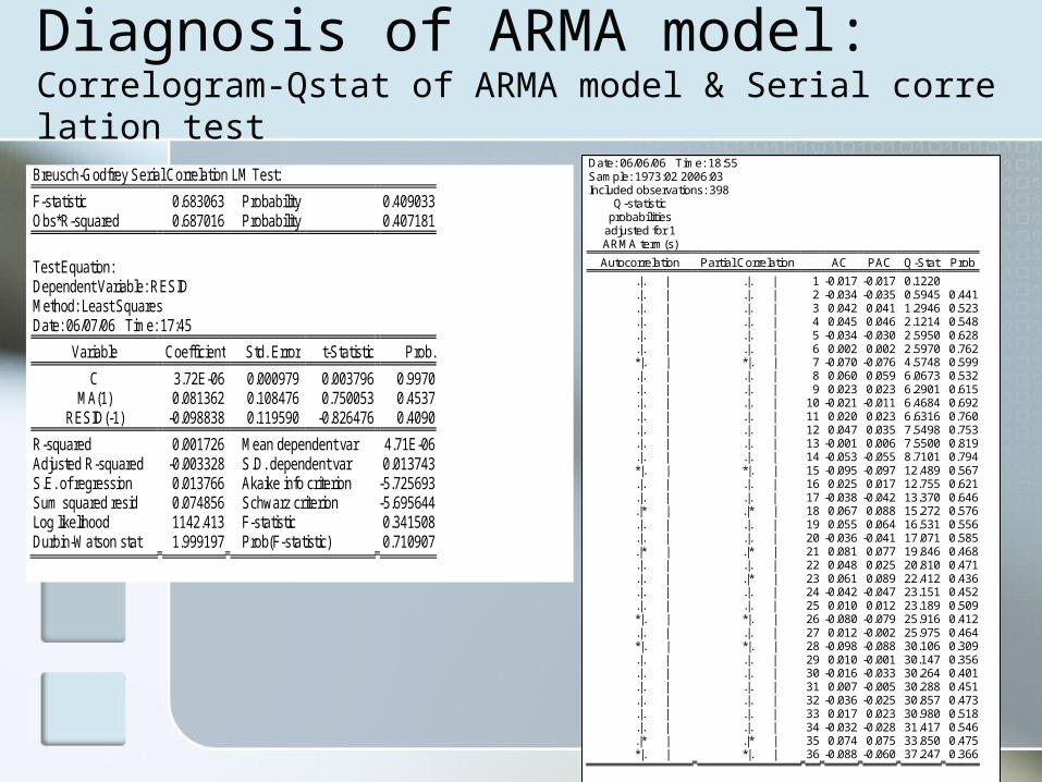
Diagnosis of ARMA model: Correlogram-Qstat of ARMA model & Serial correlation test





C 3.72E-06 0.000979 0.003796 0.9970 MA(1) 0.081362 0.108476 0.750053 0.4537

RESID(-1) -0.098838 0.119590 -0.826476 0.4090

R-squared 0.001726 Mean dependent var 4.71E-06 Adjusted R-squared -0.003328 S.D. dependent var 0.013743 S.E. of regression 0.013766 Akaike info criterion -5.725693 Sum squared resid 0.074856 Schwarz criterion -5.695644 Log likelihood 1142.413 F-statistic 0.341508 Durbin-Watson stat 1.999197 Prob(F-statistic) 0.710907





.|. | .|. | 1 -0.017 -0.017 0.1220 .|. | .|. | 2 -0.034 -0.035 0.5945 0.441 .|. | .|. | 3 0.042 0.041 1.2946 0.523 .|. | .|. | 4 0.045 0.046 2.1214 0.548 .|. | .|. | 5 -0.034 -0.030 2.5950 0.628 .|. | .|. | 6 0.002 0.002 2.5970 0.762 *|. | *|. | 7 -0.070 -0.076 4.5748 0.599 .|. | .|. | 8 0.060 0.059 6.0673 0.532 .|. | .|. | 9 0.023 0.023 6.2901 0.615 .|. | .|. | 10 -0.021 -0.011 6.4684 0.692 .|. | .|. | 11 0.020 0.023 6.6316 0.760 .|. | .|. | 12 0.047 0.035 7.5498 0.753 .|. | .|. | 13 -0.001 0.006 7.5500 0.819 .|. | .|. | 14 -0.053 -0.055 8.7101 0.794 *|. | *|. | 15 -0.095 -0.097 12.489 0.567 .|. | .|. | 16 0.025 0.017 12.755 0.621 .|. | .|. | 17 -0.038 -0.042 13.370 0.646 .|* | .|* | 18 0.067 0.088 15.272 0.576 .|. | .|. | 19 0.055 0.064 16.531 0.556 .|. | .|. | 20 -0.036 -0.041 17.071 0.585 .|* | .|* | 21 0.081 0.077 19.846 0.468 .|. | .|. | 22 0.048 0.025 20.810 0.471 .|. | .|* | 23 0.061 0.089 22.412 0.436 .|. | .|. | 24 -0.042 -0.047 23.151 0.452 .|. | .|. | 25 0.010 0.012 23.189 0.509 *|. | *|. | 26 -0.080 -0.079 25.916 0.412 .|. | .|. | 27 0.012 -0.002 25.975 0.464 *|. | *|. | 28 -0.098 -0.088 30.106 0.309 .|. | .|. | 29 0.010 -0.001 30.147 0.356 .|. | .|. | 30 -0.016 -0.033 30.264 0.401 .|. | .|. | 31 0.007 -0.005 30.288 0.451 .|. | .|. | 32 -0.036 -0.025 30.857 0.473 .|. | .|. | 33 0.017 0.023 30.980 0.518 .|. | .|. | 34 -0.032 -0.028 31.417 0.546 .|* | .|* | 35 0.074 0.075 33.850 0.475 *|. | *|. | 36 -0.088 -0.060 37.247 0.366


0.000

0.001

0.002

0.003

0.004

0.005

75 80 85 90 95 00 05

UK_RESIDSQ

0

100

200

300

400

0.000 0.001 0.002 0.003 0.004

Series: UK_RESIDSQSample 1973:02 2006:03Observations 398

Mean 0.000188Median 6.12E-05Maximum 0.004499Minimum 3.41E-10Std. Dev. 0.000377Skewness 5.743334Kurtosis 52.60938





.|** | .|** | 1 0.217 0.217 18.843 0.000 .|* | .|* | 2 0.143 0.100 27.007 0.000 .|** | .|** | 3 0.323 0.290 69.147 0.000 .|** | .|* | 4 0.235 0.130 91.542 0.000 .|* | .|. | 5 0.084 -0.029 94.413 0.000 .|* | .|. | 6 0.122 0.001 100.50 0.000 .|* | .|* | 7 0.184 0.072 114.23 0.000 .|. | .|. | 8 0.044 -0.046 115.01 0.000 .|. | .|. | 9 0.035 -0.019 115.51 0.000 .|. | .|. | 10 0.042 -0.047 116.25 0.000 .|. | .|. | 11 -0.001 -0.042 116.25 0.000 .|. | .|. | 12 0.038 0.051 116.86 0.000 .|. | .|. | 13 -0.013 -0.032 116.93 0.000 .|. | .|. | 14 -0.036 -0.035 117.46 0.000 .|. | .|. | 15 -0.006 0.000 117.48 0.000 .|. | .|. | 16 -0.028 -0.022 117.82 0.000 .|. | .|. | 17 -0.025 0.018 118.07 0.000 .|. | .|. | 18 0.002 0.031 118.07 0.000 .|. | .|. | 19 0.038 0.051 118.69 0.000 .|* | .|* | 20 0.098 0.129 122.75 0.000 .|. | .|. | 21 0.039 0.014 123.39 0.000 .|. | *|. | 22 -0.006 -0.061 123.40 0.000 .|. | .|. | 23 0.042 -0.019 124.13 0.000 .|. | .|. | 24 0.034 -0.025 124.62 0.000 .|. | .|. | 25 0.045 0.045 125.50 0.000 .|. | .|. | 26 0.014 -0.017 125.58 0.000 .|. | .|. | 27 0.033 -0.014 126.06 0.000 .|. | .|. | 28 0.059 0.041 127.56 0.000 .|. | .|. | 29 0.030 0.020 127.94 0.000 .|. | .|. | 30 0.037 0.021 128.53 0.000 .|* | .|* | 31 0.095 0.073 132.47 0.000 .|. | .|. | 32 0.034 -0.033 132.98 0.000 .|. | .|. | 33 0.005 -0.020 133.00 0.000 .|. | *|. | 34 -0.012 -0.058 133.06 0.000 .|* | .|* | 35 0.083 0.072 136.10 0.000 .|. | .|. | 36 -0.001 -0.006 136.10 0.000

ARCH Test:




C 0.000148 2.07E-05 7.144864 0.0000 RESID^2(-1) 0.216843 0.049118 4.414774 0.0000

R-squared 0.047022 Mean dependent var 0.000189 Adjusted R-squared 0.044610 S.D. dependent var 0.000377 S.E. of regression 0.000369 Akaike info criterion -12.96880 Sum squared resid 5.37E-05 Schwarz criterion -12.94873 Log likelihood 2576.306 F-statistic 19.49023 Durbin-Watson stat 2.043727 Prob(F-statistic) 0.000013

ARCH-GARCH ModelDependent Variable: DUK Method: ML - ARCH Date: 06/01/06 Time: 17:56 Sample(adjusted): 1973:02 2006:03 Included observations: 398 after adjusting endpoints Convergence achieved after 18 iterations Backcast: 1973:01


C 0.000377 0.000854 0.441344 0.6590 MA(1) 0.383377 0.057601 6.655785 0.0000

Variance Equation

C 1.66E-05 7.09E-06 2.335803 0.0195 ARCH(1) 0.163613 0.045272 3.614005 0.0003

GARCH(1) 0.750933 0.065635 11.44097 0.0000







.|. | .|. | 1 -0.009 -0.009 0.0313 .|. | .|. | 2 -0.020 -0.020 0.1896 0.663 .|. | .|. | 3 0.041 0.040 0.8562 0.652 .|. | .|. | 4 -0.010 -0.010 0.8989 0.826 .|. | .|. | 5 0.009 0.011 0.9326 0.920 .|. | .|. | 6 -0.043 -0.045 1.6805 0.891 .|. | .|. | 7 0.045 0.046 2.5197 0.866 .|. | .|. | 8 0.017 0.015 2.6438 0.916 .|. | .|. | 9 0.007 0.013 2.6621 0.954 .|. | .|. | 10 0.012 0.008 2.7178 0.974 .|. | .|. | 11 -0.042 -0.041 3.4492 0.969 .|. | .|. | 12 0.016 0.013 3.5564 0.981 .|. | .|. | 13 -0.009 -0.008 3.5896 0.990 *|. | *|. | 14 -0.068 -0.065 5.4922 0.963 .|. | .|. | 15 -0.024 -0.029 5.7342 0.973 *|. | *|. | 16 -0.072 -0.074 7.8749 0.929 .|. | .|. | 17 -0.040 -0.043 8.5591 0.930 .|. | .|. | 18 0.033 0.035 9.0230 0.940 .|. | .|. | 19 0.049 0.054 10.013 0.931 .|* | .|* | 20 0.120 0.124 16.075 0.652 .|. | .|. | 21 -0.007 0.001 16.098 0.710 .|. | .|. | 22 0.016 0.016 16.201 0.758 .|. | .|. | 23 -0.034 -0.039 16.698 0.780 .|. | .|. | 24 -0.008 0.002 16.725 0.823 .|. | .|. | 25 0.017 0.010 16.850 0.855 .|. | .|. | 26 0.042 0.053 17.606 0.859 .|. | .|. | 27 0.003 -0.016 17.609 0.890 .|. | .|. | 28 0.030 0.022 17.999 0.904 .|. | .|. | 29 -0.018 -0.033 18.142 0.923 .|* | .|* | 30 0.071 0.068 20.305 0.883 .|. | .|. | 31 0.012 0.012 20.368 0.907 .|. | .|. | 32 0.014 0.020 20.451 0.926 .|. | .|. | 33 0.035 0.030 20.972 0.932 .|. | .|. | 34 -0.044 -0.025 21.800 0.932 .|. | .|. | 35 0.034 0.046 22.320 0.938 .|. | .|. | 36 0.007 0.034 22.338 0.952

0

10

20

30

40

50

-3 -2 -1 0 1 2 3


Mean 0.005895Median 0.041618Maximum 3.330211Minimum -3.048453Std. Dev. 1.000509Skewness 0.112877Kurtosis 3.546832


Forecast of UKobs UK UKF DUK DUKF UPPERUK LOWERUK

2006:03 0.565611 0.565611 -0.007718 -0.007718 NA NA 2006:04 NA 0.563229 NA -0.002382 0.583778 0.542680 2006:05 NA 0.563606 NA 0.000377 0.586288 0.540923 2006:06 NA 0.563982 NA 0.000377 0.587360 0.540605 2006:07 NA 0.564359 NA 0.000377 0.588354 0.540364 2006:08 NA 0.564736 NA 0.000377 0.589283 0.540189 2006:09 NA 0.565112 NA 0.000377 0.590153 0.540072 2006:10 NA 0.565489 NA 0.000377 0.590973 0.540005 2006:11 NA 0.565866 NA 0.000377 0.591749 0.539983 2006:12 NA 0.566243 NA 0.000377 0.592485 0.540000 2007:01 NA 0.566619 NA 0.000377 0.593186 0.540053 2007:02 NA 0.566996 NA 0.000377 0.593856 0.540136 2007:03 NA 0.567373 NA 0.000377 0.594498 0.540248 2007:04 NA 0.567750 NA 0.000377 0.595115 0.540384 2007:05 NA 0.568126 NA 0.000377 0.595710 0.540542 2007:06 NA 0.568503 NA 0.000377 0.596285 0.540721 2007:07 NA 0.568880 NA 0.000377 0.596841 0.540918 2007:08 NA 0.569257 NA 0.000377 0.597382 0.541131 2007:09 NA 0.569633 NA 0.000377 0.597907 0.541360 2007:10 NA 0.570010 NA 0.000377 0.598419 0.541601 2007:11 NA 0.570387 NA 0.000377 0.598919 0.541855 2007:12 NA 0.570763 NA 0.000377 0.599408 0.542119

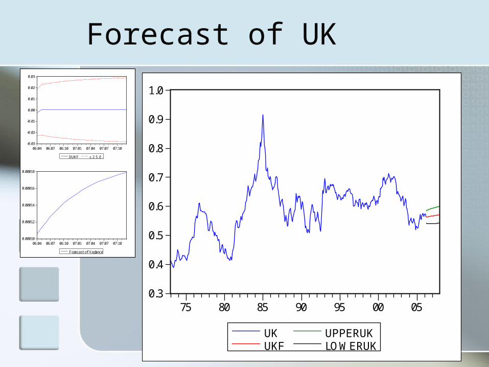
Forecast of UK

-0.03

-0.02

-0.01

0.00

0.01

0.02

0.03

06:04 06:07 06:10 07:01 07:04 07:07 07:10

DUKF ± 2 S.E.

0.00010

0.00012

0.00014

0.00016

0.00018

06:04 06:07 06:10 07:01 07:04 07:07 07:10


0.3

0.4

0.5

0.6

0.7

0.8

0.9

1.0

75 80 85 90 95 00 05

UKUKF

UPPERUKLOWERUK

Canada

Regression on Time For Canada

Dependent Variable: CANADA Method: Least Squares Date: 06/06/06 Time: 18:42 Sample(adjusted): 1973:01 2004:04 Included observations: 376 after adjusting endpoints


TIME 0.001287 4.03E-05 31.91349 0.0000 C 0.995851 0.009587 103.8770 0.0000

R-squared 0.731413 Mean dependent var Adjusted R-squared 0.730695 S.D. dependent var S.E. of regression 0.084877 Akaike info criterion Sum squared resid 2.694313 Schwarz criterion Log likelihood 394.9069 F-statistic Durbin-Watson stat 0.030197 Prob(F-statistic)

-0.3

-0.2

-0.1

0.0

0.1

0.2

0.8

1.0

1.2

1.4

1.6

1.8

75 80 85 90 95 00


Canada Series

0.8

1.0

1.2

1.4

1.6

1.8

75 80 85 90 95 00 05

CANADA

0

10

20

30

40

1.0 1.1 1.2 1.3 1.4 1.5 1.6

Series: CANADASample 1973:01 2006:03Observations 399



Correlogram and Unit root test for Canada



.|******** .|******** 1 0.991 0.991 394.90 0.000 .|******** *|. | 2 0.980 -0.110 782.26 0.000 .|*******| .|. | 3 0.970 0.005 1162.1 0.000 .|*******| .|. | 4 0.959 -0.013 1534.5 0.000 .|*******| .|. | 5 0.947 -0.042 1898.8 0.000 .|*******| .|. | 6 0.936 0.023 2255.5 0.000 .|*******| .|. | 7 0.925 0.007 2604.9 0.000 .|*******| .|. | 8 0.914 -0.006 2947.1 0.000 .|*******| .|. | 9 0.903 -0.046 3281.5 0.000 .|*******| .|. | 10 0.891 -0.031 3607.8 0.000 .|*******| *|. | 11 0.877 -0.083 3925.2 0.000 .|*******| *|. | 12 0.862 -0.071 4232.7 0.000 .|*******| .|. | 13 0.847 -0.047 4529.7 0.000 .|****** | .|. | 14 0.831 0.001 4816.5 0.000 .|****** | .|. | 15 0.815 0.009 5093.4 0.000 .|****** | .|. | 16 0.800 -0.022 5360.5 0.000 .|****** | .|. | 17 0.783 -0.035 5617.5 0.000 .|****** | .|. | 18 0.766 -0.051 5864.2 0.000 .|****** | .|. | 19 0.749 -0.030 6100.4 0.000 .|****** | .|. | 20 0.732 0.034 6326.7 0.000 .|****** | .|. | 21 0.715 0.009 6543.4 0.000 .|***** | .|. | 22 0.699 -0.006 6750.6 0.000 .|***** | .|. | 23 0.683 0.035 6948.8 0.000 .|***** | .|. | 24 0.667 0.034 7138.8 0.000 .|***** | .|. | 25 0.652 -0.014 7320.6 0.000 .|***** | .|. | 26 0.637 -0.011 7494.5 0.000 .|***** | .|. | 27 0.622 0.029 7660.8 0.000 .|***** | *|. | 28 0.606 -0.062 7819.2 0.000 .|**** | .|. | 29 0.590 -0.004 7969.8 0.000 .|**** | .|. | 30 0.574 -0.033 8112.5 0.000 .|**** | .|. | 31 0.557 0.003 8247.6 0.000 .|**** | .|. | 32 0.542 0.034 8375.7 0.000 .|**** | .|. | 33 0.527 -0.036 8497.1 0.000 .|**** | .|. | 34 0.511 -0.047 8611.5 0.000 .|**** | .|. | 35 0.495 -0.016 8719.3 0.000 .|**** | .|. | 36 0.479 0.000 8820.6 0.000

ADF Test Statistic -1.527677 1% Critical Value* 5% Critical Value 10% Critical Value


Augmented Dickey-Fuller Test Equation Dependent Variable: D(CANADA) Method: Least Squares Date: 06/06/06 Time: 18:47 Sample(adjusted): 1973:01 2006:03 Included observations: 399 after adjusting endpoints


CANADA(-1) -0.007286 0.004770 -1.527677 0.1274 C 0.009580 0.006082 1.575282 0.1160

R-squared 0.005844 Mean dependent var Adjusted R-squared 0.003340 S.D. dependent var S.E. of regression 0.015239 Akaike info criterion Sum squared resid 0.092198 Schwarz criterion Log likelihood 1104.212 F-statistic Durbin-Watson stat 1.547542 Prob(F-statistic)

First Differencing

-0.08

-0.06

-0.04

-0.02

0.00

0.02

0.04

0.06

75 80 85 90 95 00 05

DCANADA

0

20

40

60

80

-0.06 -0.04 -0.02 0.00 0.02 0.04

Series: DCANADASample 1973:02 2006:03Observations 398



Correlogram and Unit root test for DCanada



.|** | .|** | 1 0.224 0.224 20.144 0.000 .|. | .|. | 2 0.001 -0.052 20.144 0.000 .|. | .|. | 3 0.024 0.037 20.372 0.000 .|* | .|. | 4 0.070 0.059 22.358 0.000 .|. | .|. | 5 -0.011 -0.042 22.410 0.000 .|. | .|. | 6 -0.029 -0.014 22.743 0.001 .|. | .|. | 7 0.009 0.016 22.774 0.002 .|* | .|* | 8 0.093 0.087 26.270 0.001 .|* | .|. | 9 0.078 0.044 28.743 0.001 .|* | .|* | 10 0.177 0.167 41.571 0.000 .|* | .|* | 11 0.148 0.077 50.568 0.000 .|. | .|. | 12 0.034 -0.019 51.056 0.000 .|. | .|. | 13 -0.043 -0.051 51.833 0.000 .|. | .|. | 14 -0.014 -0.014 51.914 0.000 .|. | .|. | 15 -0.017 -0.023 52.027 0.000 .|. | .|* | 16 0.054 0.076 53.260 0.000 .|* | .|. | 17 0.078 0.065 55.807 0.000 .|* | .|* | 18 0.131 0.089 62.953 0.000 .|. | *|. | 19 0.013 -0.068 63.028 0.000 .|. | .|. | 20 -0.002 -0.039 63.030 0.000 .|. | .|. | 21 0.038 0.002 63.642 0.000 .|. | .|. | 22 -0.020 -0.054 63.817 0.000 .|. | .|. | 23 -0.052 -0.001 64.958 0.000 .|. | .|. | 24 -0.039 -0.010 65.613 0.000 .|. | .|. | 25 -0.005 0.000 65.624 0.000 .|. | *|. | 26 -0.029 -0.071 65.994 0.000 .|* | .|* | 27 0.106 0.104 70.838 0.000 .|. | .|. | 28 0.049 -0.049 71.855 0.000 .|. | .|. | 29 0.061 0.060 73.474 0.000 .|. | .|. | 30 -0.014 -0.018 73.564 0.000 *|. | *|. | 31 -0.075 -0.068 75.991 0.000 .|. | .|* | 32 0.054 0.105 77.264 0.000 .|. | .|. | 33 0.008 -0.022 77.292 0.000 .|. | .|. | 34 -0.046 -0.022 78.208 0.000 .|. | .|. | 35 -0.013 -0.007 78.287 0.000 *|. | *|. | 36 -0.058 -0.083 79.787 0.000



Augmented Dickey-Fuller Test Equation Dependent Variable: D(DCANADA) Method: Least Squares Date: 06/06/06 Time: 18:50 Sample(adjusted): 1973:03 2006:03 Included observations: 397 after adjusting endpoints


DCANADA(-1) -0.775425 0.049082 -15.79869 0.0000 C 0.000280 0.000750 0.373275 0.7091

R-squared 0.387216 Mean dependent var -3.60E-05 Adjusted R-squared 0.385664 S.D. dependent var 0.019049 S.E. of regression 0.014931 Akaike info criterion -5.565764 Sum squared resid 0.088056 Schwarz criterion -5.545694 Log likelihood 1106.804 F-statistic 249.5986 Durbin-Watson stat 1.973862 Prob(F-statistic) 0.000000


Dependent Variable: DCANADA Method: Least Squares Date: 06/06/06 Time: 18:29 Sample(adjusted): 1973:03 2006:03 Included observations: 397 after adjusting endpoints Convergence achieved after 4 iterations Backcast: 1972:05 1973:02


C 0.000326 0.001071 0.303880 0.7614 AR(1) 0.201986 0.049423 4.086916 0.0001

MA(10) 0.155651 0.050180 3.101837 0.0021


Inverted AR Roots .20 Inverted MA Roots .79+.26i .79 -.26i .49+.67i .49 -.67i

.00+.83i -.00 -.83i -.49 -.67i -.49+.67i -.79 -.26i -.79+.26i

-0.10

-0.05

0.00

0.05

-0.10

-0.05

0.00

0.05

75 80 85 90 95 00 05


0

20

40

60

80

-0.06 -0.04 -0.02 0.00 0.02 0.04


Mean 2.39E-06Median 0.000234Maximum 0.043689Minimum -0.073012Std. Dev. 0.014744Skewness -0.319998Kurtosis 4.212402


Diagnosis of ARMA model: Correlogram-Qstat of ARMA model & Serial correlation test





C -5.61E-06 0.001070 -0.005245 0.9958 AR(1) 0.941949 1.210177 0.778357 0.4368

MA(10) 0.004786 0.050232 0.095276 0.9241 RESID(-1) -0.926659 1.208249 -0.766944 0.4436 RESID(-2) -0.259075 0.249798 -1.037141 0.3003

R-squared 0.006369 Mean dependent var 2.39E-06 Adjusted R-squared -0.003770 S.D. dependent var 0.014744 S.E. of regression 0.014772 Akaike info criterion -5.579623 Sum squared resid 0.085542 Schwarz criterion -5.529447 Log likelihood 1112.555 F-statistic 0.628210 Durbin-Watson stat 2.006151 Prob(F-statistic) 0.642632





.|. | .|. | 1 0.012 0.012 0.0593 *|. | *|. | 2 -0.068 -0.068 1.9193 .|. | .|. | 3 0.021 0.023 2.0962 0.148 .|* | .|* | 4 0.084 0.079 4.9097 0.086 .|. | .|. | 5 -0.014 -0.013 4.9852 0.173 .|. | .|. | 6 -0.052 -0.042 6.0993 0.192 .|. | .|. | 7 -0.012 -0.016 6.1554 0.291 .|* | .|* | 8 0.078 0.068 8.6455 0.195 .|. | .|. | 9 0.030 0.031 9.0134 0.252 .|. | .|. | 10 -0.002 0.014 9.0147 0.341 .|* | .|* | 11 0.109 0.112 13.904 0.126 .|. | .|. | 12 0.032 0.015 14.315 0.159 .|. | .|. | 13 -0.050 -0.043 15.356 0.167 .|. | .|. | 14 -0.010 -0.005 15.402 0.220 .|. | .|. | 15 -0.027 -0.046 15.703 0.266 .|. | .|. | 16 0.065 0.064 17.436 0.234 .|. | .|. | 17 0.030 0.039 17.809 0.273 .|* | .|* | 18 0.110 0.128 22.899 0.116 .|. | .|. | 19 -0.023 -0.038 23.117 0.145 .|. | .|. | 20 -0.008 -0.021 23.147 0.185 .|. | .|. | 21 0.048 0.036 24.099 0.192 .|. | *|. | 22 -0.036 -0.063 24.651 0.215 .|. | .|. | 23 -0.033 -0.012 25.118 0.242 .|. | .|. | 24 -0.022 -0.012 25.331 0.281 .|. | .|. | 25 0.015 0.007 25.422 0.329 *|. | *|. | 26 -0.058 -0.070 26.874 0.310 .|* | .|* | 27 0.105 0.102 31.600 0.170 .|. | .|. | 28 0.016 -0.006 31.706 0.203 .|. | .|. | 29 0.055 0.039 33.028 0.196 .|. | .|. | 30 -0.014 -0.004 33.112 0.232 *|. | *|. | 31 -0.100 -0.092 37.475 0.134 .|* | .|* | 32 0.076 0.069 39.968 0.105 .|. | .|. | 33 0.008 0.002 39.998 0.129 .|. | .|. | 34 -0.047 -0.024 40.942 0.134 .|. | .|. | 35 0.000 0.005 40.942 0.161 .|. | *|. | 36 -0.044 -0.086 41.800 0.168


0.000

0.001

0.002

0.003

0.004

0.005

0.006

75 80 85 90 95 00 05

CANADARESSQ

0

50

100

150

200

250

300

0.000 0.001 0.002 0.003 0.004 0.005

Series: CANADARESSQSample 1973:03 2006:03Observations 397

Mean 0.000217Median 7.62E-05Maximum 0.005331Minimum 6.41E-10Std. Dev. 0.000389Skewness 6.704986Kurtosis 78.56282





.|* | .|* | 1 0.145 0.145 8.4655 0.004 .|** | .|* | 2 0.210 0.193 26.145 0.000 .|* | .|. | 3 0.073 0.022 28.312 0.000 .|* | .|* | 4 0.183 0.139 41.748 0.000 .|* | .|* | 5 0.186 0.143 55.722 0.000 .|. | *|. | 6 0.038 -0.060 56.297 0.000 .|. | .|. | 7 0.061 -0.004 57.790 0.000 .|. | .|. | 8 0.060 0.032 59.259 0.000 .|** | .|** | 9 0.251 0.207 85.071 0.000 .|. | *|. | 10 0.023 -0.063 85.293 0.000 .|. | .|. | 11 0.050 -0.030 86.305 0.000 .|* | .|* | 12 0.130 0.136 93.291 0.000 .|* | .|. | 13 0.096 0.002 97.083 0.000 .|* | .|. | 14 0.106 -0.009 101.75 0.000 .|. | .|. | 15 0.002 -0.012 101.75 0.000 .|* | .|. | 16 0.070 0.031 103.76 0.000 .|* | .|* | 17 0.192 0.156 119.21 0.000 .|* | .|* | 18 0.180 0.075 132.71 0.000 .|. | .|. | 19 0.051 -0.030 133.80 0.000 .|* | .|. | 20 0.077 0.036 136.30 0.000 .|. | *|. | 21 0.050 -0.068 137.36 0.000 .|* | .|. | 22 0.105 0.011 142.02 0.000 .|. | .|. | 23 0.060 0.017 143.53 0.000 .|. | .|. | 24 0.043 0.020 144.30 0.000 .|. | .|. | 25 0.016 -0.031 144.41 0.000 .|* | .|. | 26 0.112 0.026 149.76 0.000 .|. | .|. | 27 0.049 -0.010 150.77 0.000 .|. | .|. | 28 0.060 0.035 152.31 0.000 .|. | .|. | 29 0.064 0.002 154.09 0.000 .|* | .|. | 30 0.075 0.024 156.51 0.000 .|* | .|* | 31 0.126 0.069 163.41 0.000 .|. | *|. | 32 -0.015 -0.085 163.51 0.000 .|. | .|. | 33 -0.005 -0.054 163.52 0.000 .|. | .|. | 34 0.007 -0.016 163.54 0.000 .|. | .|. | 35 0.054 -0.028 164.80 0.000 .|. | .|. | 36 0.022 -0.008 165.01 0.000

ARCH Test:




C 0.000151 2.37E-05 6.344117 0.0000 RESID^2(-1) 0.116771 0.049542 2.356986 0.0189 RESID^2(-2) 0.193110 0.049537 3.898308 0.0001

R-squared 0.057532 Mean dependent var 0.000218 Adjusted R-squared 0.052724 S.D. dependent var 0.000390 S.E. of regression 0.000379 Akaike info criterion -12.90827 Sum squared resid 5.64E-05 Schwarz criterion -12.87805 Log likelihood 2552.383 F-statistic 11.96463 Durbin-Watson stat 2.009167 Prob(F-statistic) 0.000009

ARCH-GARCH ModelDependent Variable: DCANADA Method: ML - ARCH Date: 06/01/06 Time: 18:39 Sample(adjusted): 1973:03 2006:03 Included observations: 397 after adjusting endpoints Convergence achieved after 23 iterations Backcast: 1972:05 1973:02


C 0.000738 0.000908 0.812803 0.4163 AR(1) 0.195095 0.049148 3.969498 0.0001

MA(10) 0.166220 0.056212 2.957002 0.0031

Variance Equation

C 2.58E-06 9.39E-07 2.750863 0.0059 ARCH(1) 0.032331 0.017474 1.850206 0.0643

GARCH(1) 0.960044 0.017700 54.23970 0.0000


Inverted AR Roots .20 Inverted MA Roots .79+.26i .79 -.26i .49+.68i .49 -.68i

.00+.84i -.00 -.84i -.49 -.68i -.49+.68i -.79 -.26i -.79+.26i

0

10

20

30

40

50

-4 -3 -2 -1 0 1 2 3


Mean -0.001297Median -0.014917Maximum 3.189884Minimum -4.241014Std. Dev. 0.999969Skewness -0.071529Kurtosis 3.444506






.|. | .|. | 1 0.038 0.038 0.5714 .|* | .|* | 2 0.081 0.079 3.1878 .|. | .|. | 3 -0.023 -0.029 3.3920 0.066 .|. | .|. | 4 0.018 0.013 3.5160 0.172 .|. | .|. | 5 0.008 0.011 3.5389 0.316 .|. | .|. | 6 -0.050 -0.055 4.5627 0.335 .|. | .|. | 7 -0.015 -0.012 4.6540 0.460 *|. | .|. | 8 -0.066 -0.057 6.4216 0.378 .|* | .|* | 9 0.101 0.107 10.622 0.156 .|. | .|. | 10 -0.040 -0.039 11.287 0.186 .|. | .|. | 11 -0.016 -0.031 11.387 0.250 .|. | .|. | 12 -0.007 0.006 11.410 0.327 .|. | .|. | 13 -0.040 -0.044 12.081 0.358 .|. | .|. | 14 -0.035 -0.041 12.597 0.399 .|. | .|. | 15 -0.031 -0.012 12.996 0.448 .|. | .|. | 16 -0.029 -0.027 13.335 0.500 .|* | .|* | 17 0.066 0.084 15.160 0.440 .|. | .|. | 18 0.027 0.009 15.466 0.491 .|. | .|. | 19 -0.018 -0.031 15.606 0.552 .|. | .|. | 20 -0.004 -0.001 15.613 0.620 .|. | .|. | 21 0.004 -0.004 15.619 0.683 .|. | .|. | 22 -0.008 -0.011 15.648 0.738 .|. | .|. | 23 -0.030 -0.022 16.030 0.768 .|. | .|. | 24 -0.014 -0.010 16.117 0.810 .|. | .|. | 25 -0.024 -0.008 16.365 0.839 .|. | .|. | 26 0.031 0.014 16.762 0.859 .|. | .|. | 27 0.001 -0.003 16.763 0.890 .|. | .|. | 28 -0.007 -0.006 16.786 0.915 .|. | .|. | 29 -0.016 -0.021 16.892 0.934 .|. | .|. | 30 0.032 0.034 17.333 0.942 .|. | .|. | 31 0.060 0.064 18.886 0.924 .|. | .|. | 32 -0.045 -0.052 19.781 0.922 *|. | *|. | 33 -0.067 -0.071 21.709 0.892 .|. | .|. | 34 0.008 0.023 21.734 0.914 .|. | .|. | 35 -0.004 -0.013 21.740 0.933 .|. | .|. | 36 -0.017 -0.020 21.872 0.946

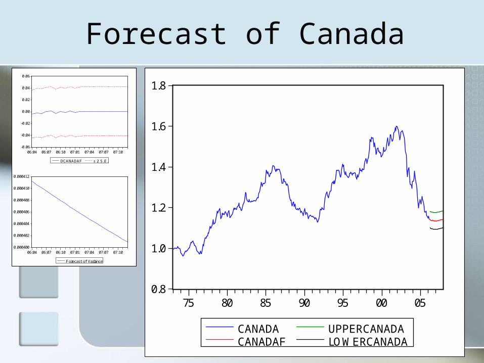
Forecast of Canada obs CANADA CANADAF DCANADA DCANADAF UPPERCANA

DA LOWERCANA

DA 2006:03 1.144100 1.144100 -0.013200 -0.013200 NA NA 2006:04 NA 1.140288 NA -0.003812 1.180844 1.099731 2006:05 NA 1.138555 NA -0.001733 1.179850 1.097261 2006:06 NA 1.136012 NA -0.002544 1.177307 1.094716 2006:07 NA 1.136136 NA 0.000124 1.177405 1.094866 2006:08 NA 1.137336 NA 0.001200 1.178578 1.096094 2006:09 NA 1.134309 NA -0.003026 1.175524 1.093094 2006:10 NA 1.135040 NA 0.000731 1.176228 1.093852 2006:11 NA 1.133637 NA -0.001404 1.174798 1.092475 2006:12 NA 1.134986 NA 0.001349 1.176121 1.093851 2007:01 NA 1.133833 NA -0.001153 1.174941 1.092724 2007:02 NA 1.134202 NA 0.000369 1.175834 1.092570 2007:03 NA 1.134868 NA 0.000666 1.176494 1.093242 2007:04 NA 1.135592 NA 0.000724 1.177193 1.093991 2007:05 NA 1.136327 NA 0.000735 1.177902 1.094752 2007:06 NA 1.137065 NA 0.000738 1.178614 1.095516 2007:07 NA 1.137803 NA 0.000738 1.179326 1.096279 2007:08 NA 1.138541 NA 0.000738 1.180039 1.097043 2007:09 NA 1.139279 NA 0.000738 1.180752 1.097806 2007:10 NA 1.140017 NA 0.000738 1.181465 1.098569 2007:11 NA 1.140755 NA 0.000738 1.182178 1.099332 2007:12 NA 1.141493 NA 0.000738 1.182891 1.100095

Forecast of Canada

-0.06

-0.04

-0.02

0.00

0.02

0.04

0.06

06:04 06:07 06:10 07:01 07:04 07:07 07:10

DCANADAF ± 2 S.E.

0.000400

0.000402

0.000404

0.000406

0.000408

0.000410

0.000412

06:04 06:07 06:10 07:01 07:04 07:07 07:10


0.8

1.0

1.2

1.4

1.6

1.8

75 80 85 90 95 00 05

CANADACANADAF

UPPERCANADALOWERCANADA

Conclusion

Each of the four set shows a similar posture as against time

Foreign exchange rate measures the country’s economic strength and currency purchasing power

U.S. dollar may stay under pressure in the future year, it probably going to be less demand in Asian market, but it should be doing fine in Europe and North America

The End

Documents

Exchange Rate YuYuan Liu Han Yu Yang Dennis Yue Jessica Chen Jo-Yu Mao