Excel: Tutorial Week 3 - University of Calgary in Alberta

10/18/2020

Excel: 1

Excel: Tutorial Week 3

• Lookup tables and lookup functions

• Counting occurrences

• The column chart

• Branching and logic

• Logic and web searches: AND, OR, NOT (subtraction)

• Cell references: more advanced examples, transposing their use

• Finding and fixing errors

Official resource for MS-Office products: https://support.office.com

First Tutorial

10/18/2020

Excel: 2

MS-Excel tutorial notes by James Tam

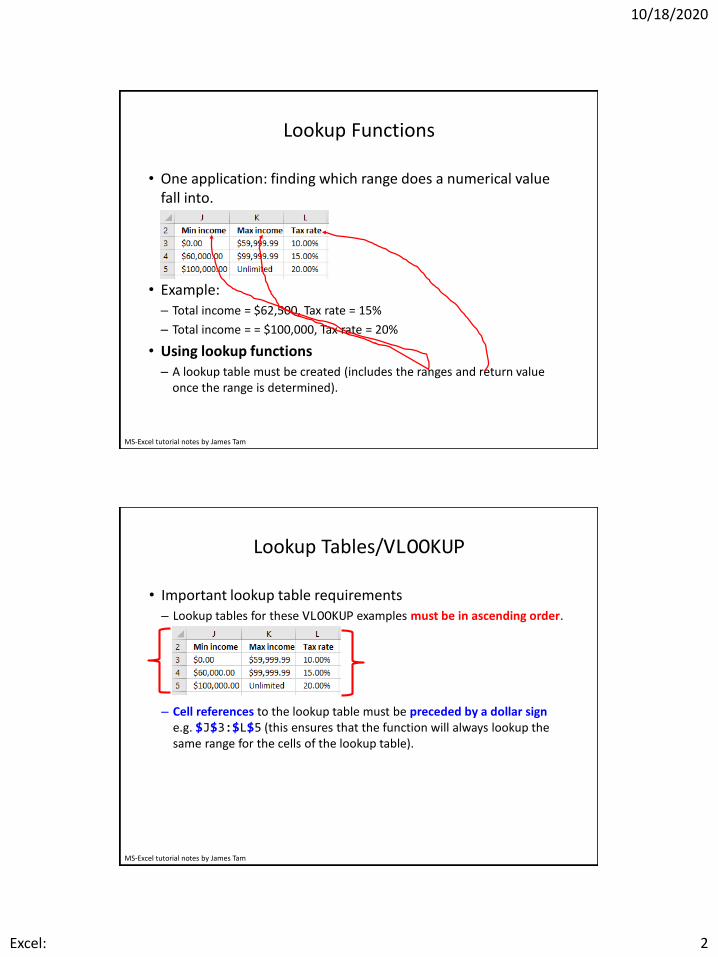
Lookup Functions

• One application: finding which range does a numerical value fall into.

• Example:– Total income = $62,500, Tax rate = 15%

– Total income = = $100,000, Tax rate = 20%

• Using lookup functions– A lookup table must be created (includes the ranges and return value

once the range is determined).


Lookup Tables/VLOOKUP

• Important lookup table requirements– Lookup tables for these VLOOKUP examples must be in ascending order.

– Cell references to the lookup table must be preceded by a dollar sign e.g. $J$3:$L$5 (this ensures that the function will always lookup the same range for the cells of the lookup table).

10/18/2020

Excel: 3


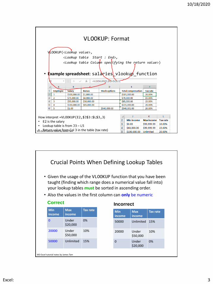
VLOOKUP: Format

VLOOKUP(<Lookup value>,

<Lookup table Start : End>,

<Lookup table Column specifying the return value>)

• Example spreadsheet: salaries_vlookup_function

How interpret =VLOOKUP(E2,$J$3:$L$3,3)• E2 is the salary• Lookup table is from J3 – L5• Return value from Col 3 in the table (tax rate)


Crucial Points When Defining Lookup Tables

• Given the usage of the VLOOKUP function that you have been taught (finding which range does a numerical value fall into) your lookup tables must be sorted in ascending order.

• Also the values in the first column can only be numeric

Min income

Max income

Tax rate

0 Under$20,000

0%

20000 Under$50,000

10%

50000 Unlimited 15%

Correct

Min income

Max income

Tax rate

50000 Unlimited 15%

20000 Under$50,000

10%

0 Under$20,000

0%

Incorrect

10/18/2020

Excel: 4


Types Of Formula Errors In Excel

• Syntax error (occurs when the syntax, or rules, of defining the formula have been violated):– A pre-created Excel formula is incorrectly named or has incorrect

arguments e.g. =AVERIGE(A1:F10), =IF("Hello",C2,A2)

– Excel will provide clues when a syntax error has occurred.

– #NAME? (There is no formula named ‘AVERIGE’)

– #VALUE! (A value or argument has been specified incorrectly)

• Logic error (occurs when the logic, or value produced, by the formula is wrong):– A formula is specified incorrectly e.g. area of a rectangular property is

specified using addition rather than multiplication (=A1+B1)

– Logic errors are more difficult to find and fix.


Finding And Fixing Logic Errors

• Testing the formula is one approach for ‘debugging’/finding & fixing the error/bug (e.g. enter 4 and 3 into Cells A1 and B1respectively and see if the expected value of 12 is returned by the formula– This error is easy to catch, not all logic errors will be this easy.

• That’s why there are bugs in actual commercial programs.

– Two things to look for when debugging logic errors:

1. Check the input data is correct

• E.g. area of circle: A = Π * r2, A = 1.34 * 102 incorrectly uses 1.34 instead of 3.14

2. Check the formula is correctly specified

• E.g. area of a rectangle = width * length, A = w + l incorrectly uses addition instead of multiplication

10/18/2020

Excel: 5


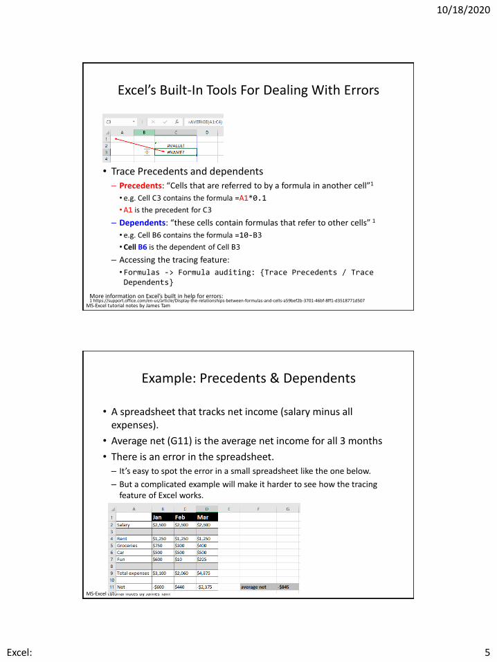
Excel’s Built-In Tools For Dealing With Errors

• Trace Precedents and dependents – Precedents: “Cells that are referred to by a formula in another cell”1

• e.g. Cell C3 contains the formula =A1*0.1

• A1 is the precedent for C3

– Dependents: “these cells contain formulas that refer to other cells” 1

• e.g. Cell B6 contains the formula =10-B3

• Cell B6 is the dependent of Cell B3

– Accessing the tracing feature:

• Formulas -> Formula auditing: {Trace Precedents / Trace Dependents}

More information on Excel’s built in help for errors:1 https://support.office.com/en-us/article/Display-the-relationships-between-formulas-and-cells-a59bef2b-3701-46bf-8ff1-d3518771d507


Example: Precedents & Dependents

• A spreadsheet that tracks net income (salary minus all expenses).

• Average net (G11) is the average net income for all 3 months

• There is an error in the spreadsheet.– It’s easy to spot the error in a small spreadsheet like the one below.

– But a complicated example will make it harder to see how the tracing feature of Excel works.

10/18/2020

Excel: 6


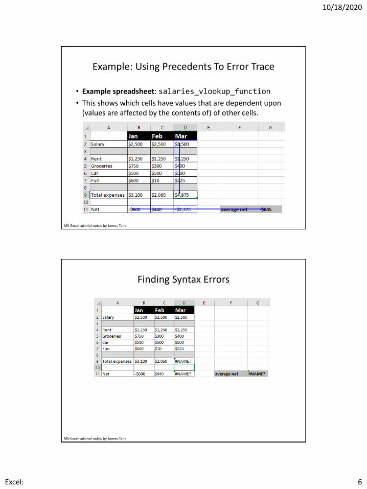
Example: Using Precedents To Error Trace

• Example spreadsheet: salaries_vlookup_function

• This shows which cells have values that are dependent upon (values are affected by the contents of) of other cells.


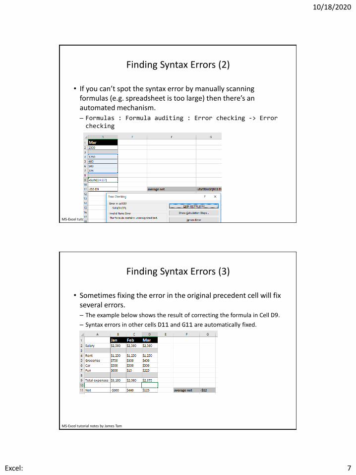
Finding Syntax Errors

10/18/2020

Excel: 7


Finding Syntax Errors (2)

• If you can’t spot the syntax error by manually scanning formulas (e.g. spreadsheet is too large) then there’s an automated mechanism.– Formulas : Formula auditing : Error checking -> Error checking


Finding Syntax Errors (3)

• Sometimes fixing the error in the original precedent cell will fix several errors.– The example below shows the result of correcting the formula in Cell D9.

– Syntax errors in other cells D11 and G11 are automatically fixed.

10/18/2020

Excel: 8


Circular References

• A specific type of error when a cell containing a formula includes that cell in the formula.

• Cell A10 contains the formula: =AVERAGE(A1:A10).


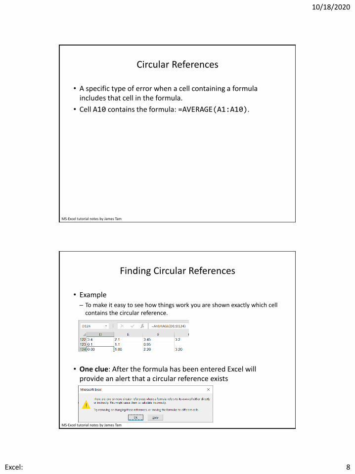
Finding Circular References

• Example– To make it easy to see how things work you are shown exactly which cell

contains the circular reference.

• One clue: After the formula has been entered Excel will provide an alert that a circular reference exists

10/18/2020

Excel: 9


Finding Circular References

• Finding the problem afterward: you can use the built in mechanism for finding circular references:

• Formulas : Calculations : Error Checking -> Circular references


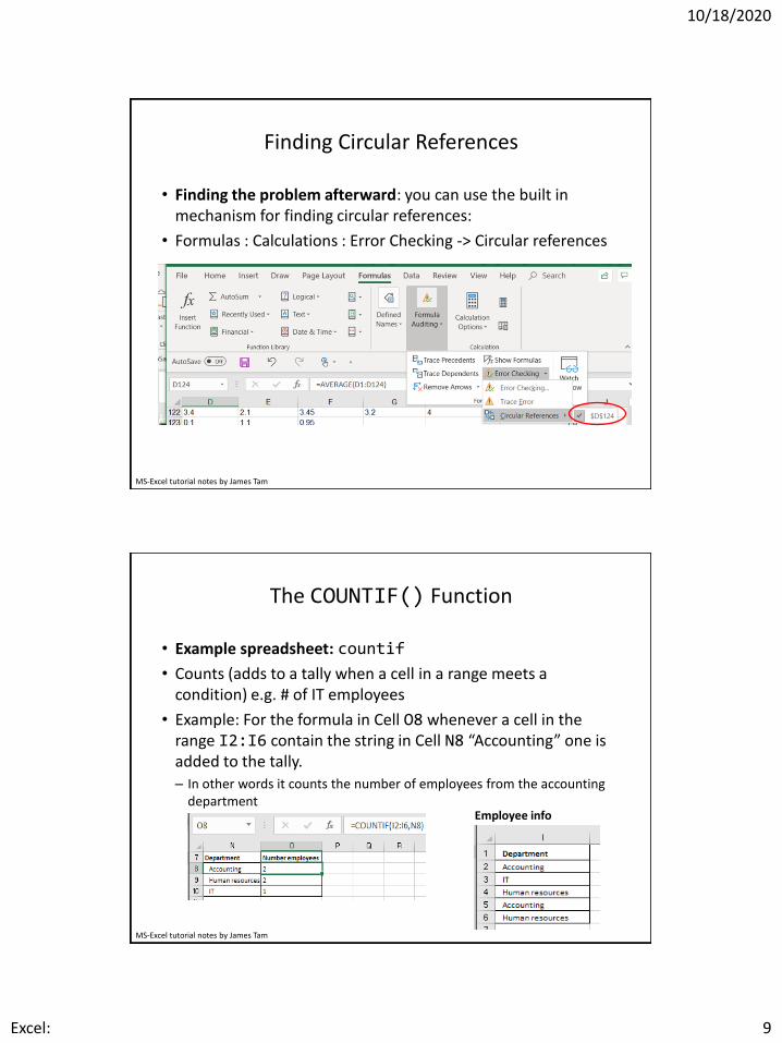
The COUNTIF() Function

• Example spreadsheet: countif

• Counts (adds to a tally when a cell in a range meets a condition) e.g. # of IT employees

• Example: For the formula in Cell O8 whenever a cell in the range I2:I6 contain the string in Cell N8 “Accounting” one is added to the tally.– In other words it counts the number of employees from the accounting

departmentEmployee info

10/18/2020

Excel: 10


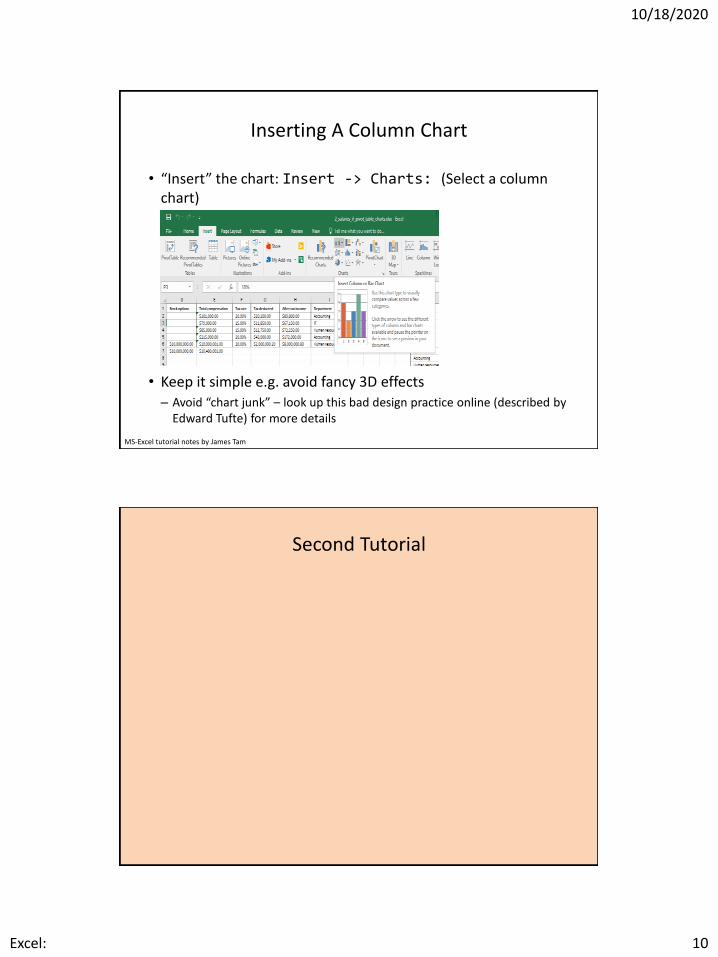
Inserting A Column Chart

• “Insert” the chart: Insert -> Charts: (Select a column chart)

• Keep it simple e.g. avoid fancy 3D effects– Avoid “chart junk” – look up this bad design practice online (described by

Edward Tufte) for more details

Second Tutorial

10/18/2020

Excel: 11


The IF() Function

• It operates in a similar fashion to conditional formatting and the COUNTIF() function: is it true that some condition has been met.

• Unlike the formatting feature and the COUNTIF() function the return value can be specified:– A constant e.g. number, text string, Boolean (12, -12, 1.5, “Pass”, True etc.)…any value that be typed into an Excel cell can be the specified constant.

– A reference to a cell (and that cell can then contain one of the above values).

– An expression that evaluates to any one of the above values e.g. 2*3, “hi”&”there”


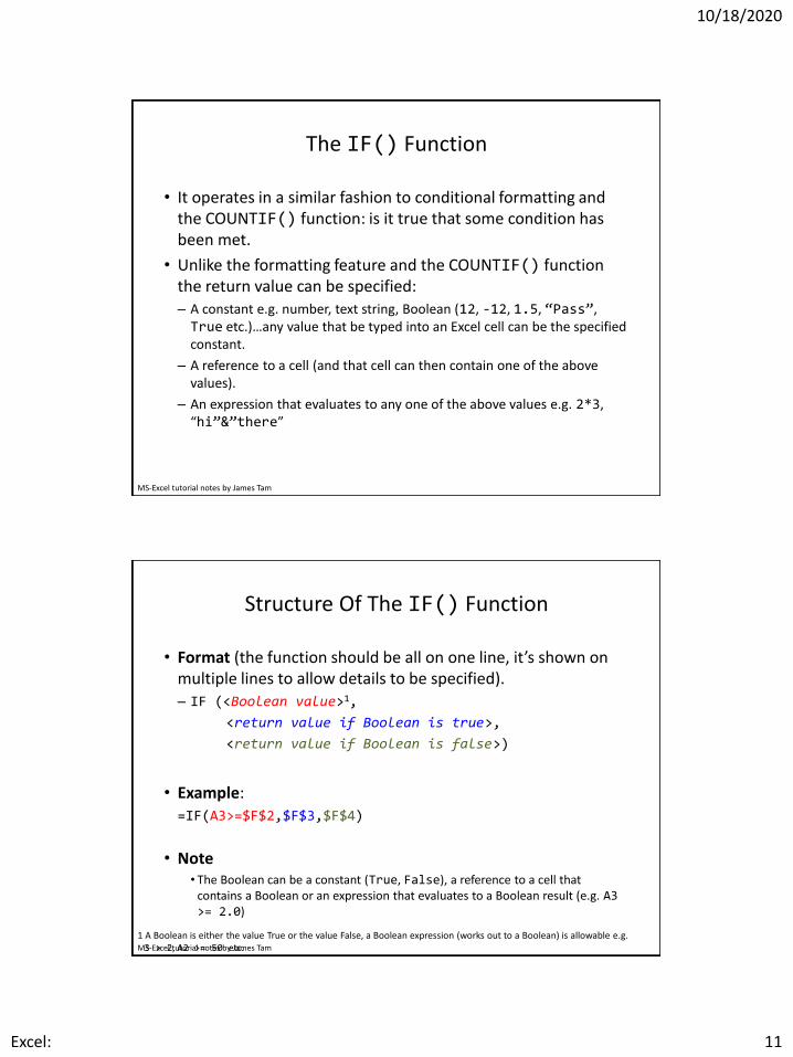
Structure Of The IF() Function

• Format (the function should be all on one line, it’s shown on multiple lines to allow details to be specified).– IF (<Boolean value>1,

<return value if Boolean is true>,

<return value if Boolean is false>)

• Example:=IF(A3>=$F$2,$F$3,$F$4)

• Note• The Boolean can be a constant (True, False), a reference to a cell that

contains a Boolean or an expression that evaluates to a Boolean result (e.g. A3 >= 2.0)

1 A Boolean is either the value True or the value False, a Boolean expression (works out to a Boolean) is allowable e.g. 3 > 2, A2 >= 50 etc.

10/18/2020

Excel: 12


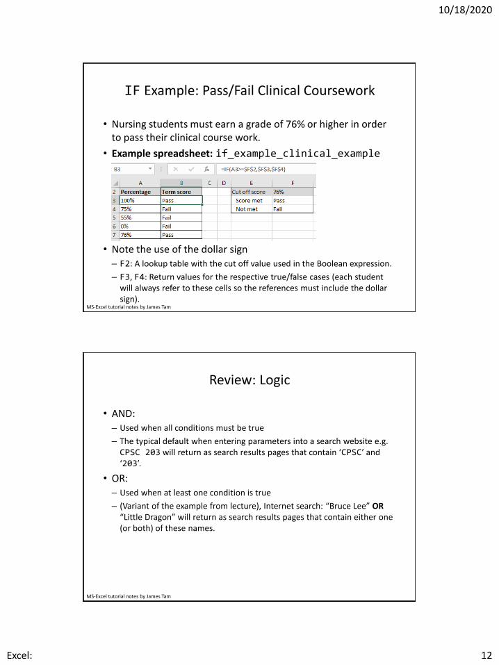
IF Example: Pass/Fail Clinical Coursework

• Nursing students must earn a grade of 76% or higher in order to pass their clinical course work.

• Example spreadsheet: if_example_clinical_example

• Note the use of the dollar sign – F2: A lookup table with the cut off value used in the Boolean expression.

– F3, F4: Return values for the respective true/false cases (each student will always refer to these cells so the references must include the dollar sign).


Review: Logic

• AND:– Used when all conditions must be true

– The typical default when entering parameters into a search website e.g. CPSC 203 will return as search results pages that contain ‘CPSC’ and ‘203’.

• OR:– Used when at least one condition is true

– (Variant of the example from lecture), Internet search: “Bruce Lee” OR“Little Dragon” will return as search results pages that contain either one (or both) of these names.

10/18/2020

Excel: 13


Logical ‘AND’ & Web Searches: Student Exercise

• Search case #1, type the following into a search site:– coronavirus cases

– Note the number of search results

• Search case #2, type the following into a search site:– coronavirus cases Canada

– Note the number of search results (increased or decreased?)


Logical ‘OR’ & Web Searches

• Search case #1, type the following into a search site:– “Calgary headlines" “Edmonton headlines”

– Note the number of search results

• Search case #2, type the following into a search site:– “Calgary headlines" OR “Edmonton headlines” (OR is case sensitive)


• Search case #3, type the following into a search site:– “Calgary headlines" or “Edmonton headlines” (OR is case sensitive)


10/18/2020

Excel: 14


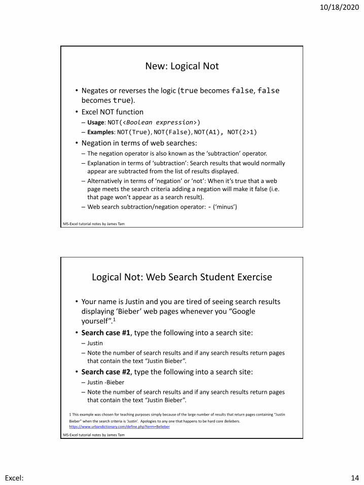
New: Logical Not

• Negates or reverses the logic (true becomes false, falsebecomes true).

• Excel NOT function– Usage: NOT(<Boolean expression>)

– Examples: NOT(True), NOT(False), NOT(A1), NOT(2>1)

• Negation in terms of web searches:– The negation operator is also known as the ‘subtraction’ operator.

– Explanation in terms of ‘subtraction’: Search results that would normally appear are subtracted from the list of results displayed.

– Alternatively in terms of ‘negation’ or ‘not’: When it’s true that a web page meets the search criteria adding a negation will make it false (i.e. that page won’t appear as a search result).

– Web search subtraction/negation operator: - (‘minus’)


Logical Not: Web Search Student Exercise

• Your name is Justin and you are tired of seeing search results displaying ‘Bieber’ web pages whenever you “Google yourself”.1

• Search case #1, type the following into a search site:– Justin

– Note the number of search results and if any search results return pages that contain the text “Justin Bieber”.

• Search case #2, type the following into a search site:– Justin -Bieber

– Note the number of search results and if any search results return pages that contain the text “Justin Bieber”.

1 This example was chosen for teaching purposes simply because of the large number of results that return pages containing “Justin

Bieber” when the search criteria is ‘Justin’. Apologies to any one that happens to be hard core Beliebers.

https://www.urbandictionary.com/define.php?term=Belieber

https://www.urbandictionary.com/define.php?term=Belieber

10/18/2020

Excel: 15


Interested In Advanced Web Searches?

• For more information:– https://pages.cpsc.ucalgary.ca/~tamj/2020/203W/notes/pdf/Internet_se

arching.pdf


Using The Logical Functions (AND, OR) In Excel

• Format:AND(<True or False>,<True or False>...)

OR(<True or False>,<True or False>...)

• Types of inputs:– A constant value (False, True)

– A cell reference (e.g. A2, BB64 etc.)

– An expression that evaluates to True or False result (e.g. 3 > 2, A2 >= 50 etc.)

• Examples:– AND(False,True,False)

– AND(B1,True)

– OR(False,False,True)

• Exercise: what does this function return?– OR(B1>B2,B2>B1)

https://pages.cpsc.ucalgary.ca/~tamj/2020/203W/notes/pdf/Internet_searching.pdf

10/18/2020

Excel: 16


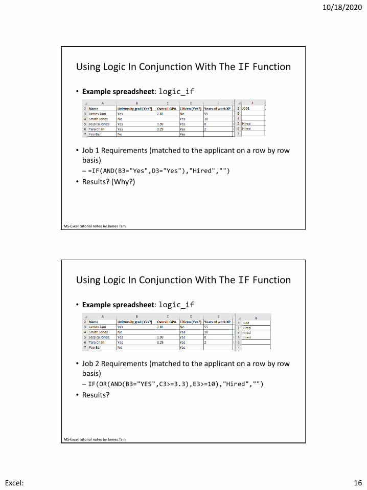
Using Logic In Conjunction With The IF Function

• Example spreadsheet: logic_if

• Job 1 Requirements (matched to the applicant on a row by row basis)– =IF(AND(B3="Yes",D3="Yes"),"Hired","")

• Results? (Why?)


Using Logic In Conjunction With The IF Function

• Example spreadsheet: logic_if

• Job 2 Requirements (matched to the applicant on a row by row basis)– IF(OR(AND(B3="YES",C3>=3.3),E3>=10),"Hired","")

• Results?

10/18/2020

Excel: 17


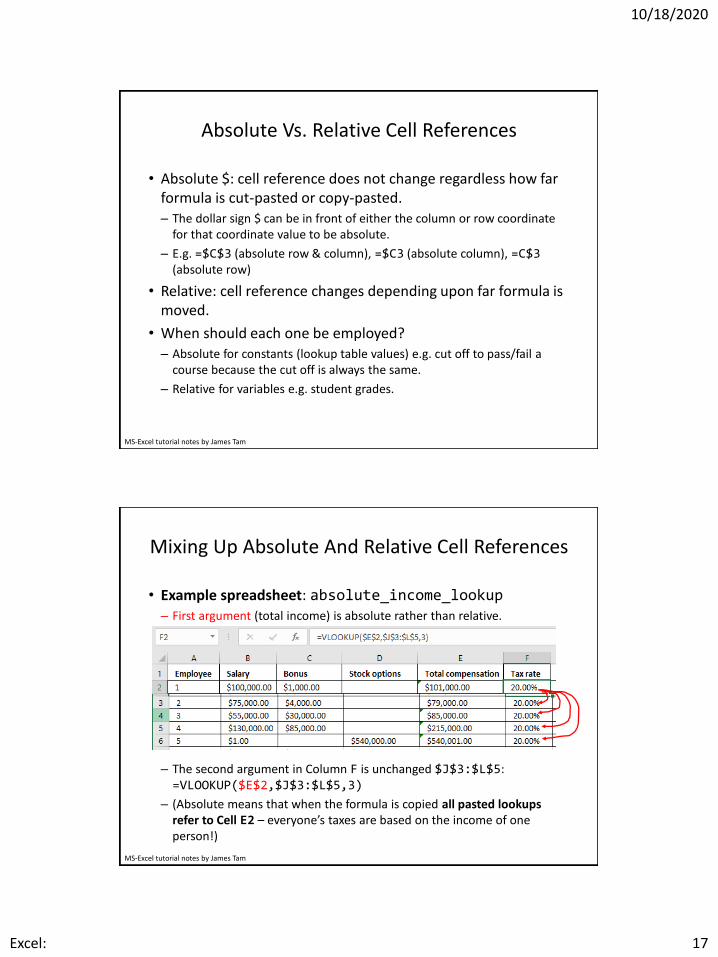
Absolute Vs. Relative Cell References

• Absolute $: cell reference does not change regardless how far formula is cut-pasted or copy-pasted.– The dollar sign $ can be in front of either the column or row coordinate

for that coordinate value to be absolute.

– E.g. =$C$3 (absolute row & column), =$C3 (absolute column), =C$3(absolute row)

• Relative: cell reference changes depending upon far formula is moved.

• When should each one be employed?– Absolute for constants (lookup table values) e.g. cut off to pass/fail a

course because the cut off is always the same.

– Relative for variables e.g. student grades.


Mixing Up Absolute And Relative Cell References

• Example spreadsheet: absolute_income_lookup– First argument (total income) is absolute rather than relative.

– The second argument in Column F is unchanged $J$3:$L$5: =VLOOKUP($E$2,$J$3:$L$5,3)

– (Absolute means that when the formula is copied all pasted lookups refer to Cell E2 – everyone’s taxes are based on the income of one person!)

10/18/2020

Excel: 18


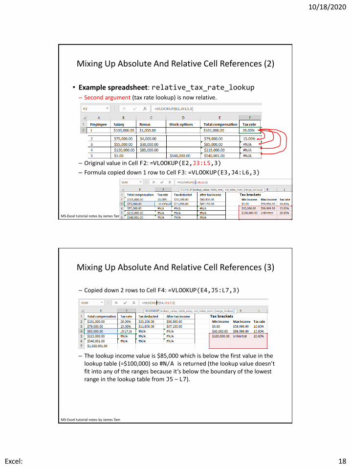
Mixing Up Absolute And Relative Cell References (2)

• Example spreadsheet: relative_tax_rate_lookup– Second argument (tax rate lookup) is now relative.

– Original value in Cell F2: =VLOOKUP(E2,J3:L5,3)

– Formula copied down 1 row to Cell F3: =VLOOKUP(E3,J4:L6,3)


Mixing Up Absolute And Relative Cell References (3)

– Copied down 2 rows to Cell F4: =VLOOKUP(E4,J5:L7,3)

– The lookup income value is $85,000 which is below the first value in the lookup table (=$100,000) so #N/A is returned (the lookup value doesn’t fit into any of the ranges because it’s below the boundary of the lowest range in the lookup table from J5 – L7).

10/18/2020

Excel: 19


Other Excel Resources

• Online training resources created by Microsoft:– Tutorials

• https://support.office.com/en-us/article/excel-for-windows-training-9bc05390-e94c-46af-a5b3-d7c22f6990bb

– A MAC specific resource

• https://support.office.com/en-us/article/excel-2016-for-mac-help-2010f16b-aec0-4da7-b381-9cc1b9b47745

https://support.office.com/en-us/article/excel-for-windows-training-9bc05390-e94c-46af-a5b3-d7c22f6990bb

https://support.office.com/en-us/article/excel-2016-for-mac-help-2010f16b-aec0-4da7-b381-9cc1b9b47745

Documents

Excel: Tutorial Week 3 - University of Calgary in Alberta