IInnttrroodduuccttiioonn ttoo

EExxcceell 22001100

Updated November 2011

Himmelfarb Health Sciences Library The George Washington University Medical Center

2300 Eye Street, NW, Washington, DC 20037 Phone: (202) 994-2850 or Email: library@gwumc.edu

Excel Handout 2

Microsoft Excel is a spreadsheet software program for use in organizing data, performing data calculations, and graphing datasets.

Basics Worksheet Layout Entering Text and Numbers Formatting Text, Numbers, and Cells

Presenting the Information Page Setup Options Printing Options Creating Charts

Using Data Shortcuts AutoFill AutoSum Formulas Fill Right Fill Down Sorting

Excel Handout 3

BASICS Worksheet Layout

Rows and Columns: Each worksheet is composed of rows (numbered) and columns (lettered).

Cells: The intersection of each row and column creates a cell. The cell is identified by its location on the worksheet (i.e. B3). An active cell is outlined in black and the location appears in the Name box (E3 is active in Fig. 1).

Worksheet/Sheets:

Each page of cells is called a worksheet or sheet. Multiple worksheets are available in each Excel file. Click on the Sheet tab to access a new worksheet. The Sheet tabs can be renamed by double-clicking on the current tab name, then typing the desired name.

Formula Bar:

The formula bar displays the contents of an individual cell. The contents may be text, numbers and/or formulas, depending on the cell.

Fig. 1

Entering Text and Numbers Moving the cursor:

You can move the cursor using several options on the keyboard:

Tab key- moves one cell to the right (along the row)

Shift-Tab keys- moves one cell to the left (along the row)

Enter key- moves one cell down (along the column)

Shift-Enter keys- moves one cell up (along the column)

Cursor keys (arrow keys)- moves one cell in direction of arrow on key

Any cell can also be activated by clicking on it using the mouse.

Entering content: Once the cursor is in the appropriate cell, enter the content using the keyboard. Cells will accept text or numbers, as well as equations (see formula section for details). There are a few default settings that become evident once there is content in a cell:

Numbers are right-justified.

Text is left-justified.

Whole numbers will not display zeros after the decimal point (unless the cell has

been specially formatted).

Excel Handout 4

Cutting and Pasting Cells: • To move a filled cell, click on the cell to activate it,

and press Ctrl-X on the keyboard (or go to the Edit menu and select Cut). The activated cell will be encircled by a flashing dotted line (Fig. 2).

• Move the cursor to the desired blank cell and press Ctrl-V (or go to the Edit menu and select Paste).

• To move a group of filled cells, hold down the left mouse button and drag the cursor over the group of cells, selecting all of them. Then complete the cut and paste commands.

Inserting Rows and Columns: To insert a column:

Fig. 2

Click the letter above the column to the left of where you want the new column to show up – this will highlight the entire column, right click your mouse and select insert

To insert a row: Click the number to the left of a row below where you want the new row to show up – this will highlight the entire row, right click your mouse and select insert

Editing Cell Content:

The contents of any cell can be edited at any time. To see the cell’s contents, click on the cell and look in the formula bar. Click with the cursor in the formula bar to add or remove content at that location.

Formatting Text, Numbers, and Cells

Selecting/Moving Rows or Columns: To select an entire row, click on the number of the row in the gray column on the left. To select an entire column, click on the letter of the column in the gray row at the top. To move the entire row or column select entire row, hold down the shift key, click on row/column line and drag it to the desired row/column.

Formatting Text:

Font/Point Size/Bold/Underline- Once the desired cell(s) have been selected, click the appropriate formatting button in the toolbar at the top of the screen (Fig. 3) to alter the appearance of the text in that cell(s).

Subscripts/superscripts- To add subscripts or superscripts to a cell, highlight the letter/number in the formula bar. Under Home Tab, Font Menu, select corner arrow that will open up the Format Cells. Check the box for superscript or subscript as desired.

Fig. 3

Excel Handout 5

Alignment-

• Left/Center/Right: To change the default horizontal alignment of a cell’s contents, select the cell(s) or row(s)/column(s), and click the appropriate alignment button on the tool bar. (Fig. 4)

Fig. 4

Left, Center, Right Alignment

• Top/Center/Bottom: To change the default vertical alignment of a cell’s contents, select the cell(s). Under the Home Tab, Alignment Menu (Fig. 5) choose the desired alignment.

Wrapping text- In some cases, the content in a cell will exceed the amount of space available. If there is extra text, only the beginning of the text will be visible. If a number is too long to fit, the cell will display #####, rather than the number. To fix this problem you could increase the width of the column (see Formatting Cells), or you can format the cell to allow the text to wrap onto a second line within the cell.

• Select the cell(s) that needs to have text on multiple lines. (Entire columns or rows can also be selected.)

• On the Home Tab select “wrap text” button.

Fig. 5

Merging and Centering cells- Sometimes text needs to be centered over multiple columns. Rather than trying to guess which column is the central one and typing the text in that column’s cell, the entire set of cells in that row can be combined.

• Select the cells.

• Click the Merge and Center button on the toolbar. (Fig.5)

• The same process can be done via the Alignment window (Fig. 5 above) by checking the Merge cells box and horizontally centering the text.

Excel Handout 6

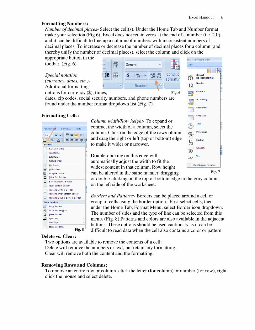
Formatting Numbers: Number of decimal places- Select the cell(s). Under the Home Tab and Number format make your selection (Fig.6). Excel does not retain zeros at the end of a number (i.e. 2.0) and it can be difficult to line up a column of numbers with inconsistent numbers of decimal places. To increase or decrease the number of decimal places for a column (and thereby unify the number of decimal places), select the column and click on the appropriate button in the

toolbar. (Fig. 6)

Special notation

(currency, dates, etc.)-

Additional formatting

options for currency ($), times,

Fig. 6

dates, zip codes, social security numbers, and phone numbers are found under the number format dropdown list (Fig. 7).

Formatting Cells:

Column width/Row height- To expand or contract the width of a column, select the column. Click on the edge of the row/column and drag the right or left (top or bottom) edge to make it wider or narrower.

Double-clicking on this edge will automatically adjust the width to fit the widest content in that column. Row height can be altered in the same manner, dragging

Fig. 7

or double-clicking on the top or bottom edge in the gray column on the left side of the worksheet.

Fig. 8

Delete vs. Clear:

Borders and Patterns- Borders can be placed around a cell or group of cells using the border option. First select cells, then under the Home Tab, Format Menu, select Border icon dropdown. The number of sides and the type of line can be selected from this menu. (Fig. 8) Patterns and colors are also available in the adjacent buttons. These options should be used cautiously as it can be difficult to read data when the cell also contains a color or pattern.

Two options are available to remove the contents of a cell: Delete will remove the numbers or text, but retain any formatting. Clear will remove both the content and the formatting.

Removing Rows and Columns:

To remove an entire row or column, click the letter (for column) or number (for row), right click the mouse and select delete.

Excel Handout 7

USING DATA SHORTCUTS

Autofill A quick shortcut to add a series of text is to use the Autofill function.

• Enter the first term in the series (i.e. January, Monday, First Quarter, etc.)

• Using the mouse, drag the small black square in the lower right corner of the cell across the rows or down the column to fill in the remaining portion of the series.

AutoSum Summing a column or row of numbers can be done easily by clicking the AutoSum button in the toolbar. (Fig. 9)

• Place the cursor in the cell that will contain the total.

• Click the AutoSum button.

Fig. 9

• The cells to be added will be enclosed in a flashing dotted line. Make sure all of the appropriate cells are included. If there are blank cells in the midst of the row or column of numbers, the outline will have to be added manually by dragging the cursor across the desired cells.

• The range of cells can also be double-checked by viewing the formula generated in the original cell. For example, to add the contents of cells B3 through B10, the generated formula should read

• Press Enter to view the total.

=SUM(B3:B10)

Formulas Excel can also perform other types of mathematical calculations including multiplication, division, and subtraction.

• To enter a formula, click in the cell that will hold the results of the equation.

• Press the equal sign to start the formula, then enter the cell names and notations to complete the formula. For example, to subtract the value of B5 from B3, the equation would read

=B3-B5 Note: Use the asterisk (*) for the multiplication symbol, and the forward slash(/) for the division symbol.

An absolute cell reference does not change, even when the formula is copied and pasted elsewhere or when a formula needs an absolute reference. Suppose in C1 you use a formula referencing A1. If you copy the formula to C2 it will reference A2 and likewise if you copy the formula to D1 it will reference B1. By adding $ in front of A and 1 then no matter where the formula is moved/copied to it will reference A1.

=$B$3-B5 Using formula wizard: SUMIF: Adds the cells specified by a given criteria (i.e. =SUMIF(B2:B25,">5")

COUNTIF: Counts the number of cells within a range that meet the given criteria (i.e. =COUNTIF(B2:B25,"Nancy")

AVERAGE: Returns the average of its arguments (=AVERAGE(A2:A6)

STD DEVIATION: Estimates the standard deviation based on a sample (=STDDEV(A2:A6)

If you need more information, go to the Microsoft Excel Help menu and search for “worksheet functions.”

Excel Handout 8

Fill (Right, Down) Once a formula has been created, it can be automatically added to adjacent cells in a row or column (adjusted for the row number or column letter).

• Put the cursor in the cell containing the formula.

• Holding the mouse button down, highlight the adjacent cells that will contain the modified formula.

• Under the Home Tab, Editing Menu, select Fill. From the submenu, select the appropriate direction (i.e. right, down, etc.).

• The formulas will be added to the cells. The formula for each of the adjacent cells can be double-checked by clicking in the cell and viewing the contents in the Formula bar. If there is no data on which to perform the calculation, the cell will contain a zero.

Sorting Once data has been entered, it is possible to sort the information into a different sequence, retaining the link between the label and the numerical information.

• Highlight the rows or columns to be sorted, clicking on the gray row number or column letter to select the entire row/column.

• Under the Home Tab, Editing Menu, select Sort & Filter (Fig. 10)

• Select how the sort should occur (ascending or descending) or you can custom sort and determine which column determines the sorting

method. (Fig.11)

Fig. 10

• Check the appropriate button to indicate whether or not a header row has been included in the highlighted rows of data.

• Click OK to perform the sort.

• Multiple-level sorts can be performed using the addition sorting levels in the window (i.e. Sort sales by month, then by salesperson).

Fig. 11

Excel Handout 9

PRESENTING THE INFORMATION

Page Setup Options Orientation

Excel spreadsheets are often wider than they are long, so many will benefit from changing the orientation of the page from portrait (vertical) to landscape (horizontal).

• Under the Page Layout Tab, Page Setup Menu.

• Click on Orientation to select Landscape orientation. (Fig. 12)

Fit to One Page Spreadsheets

can also be automatically scaled to fit onto one (or more pages). Click on the Page Layout Tab, Scale to Fit Menu and click the drop down menu to 1 page (Fig. 13). Note: The resulting text size may be quite small.

Fig. 12

Fig. 13

Margins

Margins can be altered to provide additional space for data. (Fig. 14) No margin should be smaller than .5 inches in order to avoid cutting off part of the data when printing.

Centering on Page

To center small blocks of data on the page (without altering the margins), click the appropriate box in Page Layout Tab, Page Setup Menu, Margins, Custom Margins, select horizontally or vertically. (Fig. 14)

Fig. 14

Header/Footer Headers and Footers provide a convenient location for small pieces of information. Common elements of these two text areas are page numbers, dates (creation or printing date), times, author name, version number, and/or project name. Standard options and formatting are available under the Insert Tab, Text Menu, and select Header & Footer (Fig. 15).

Fig. 15

Excel Handout 10

Sheet

If a spreadsheet spans multiple pages, it can be helpful to include the row/column containing the headings on each page. To automatically add this option, in the Page Layout Tab, Print Setup Menu, select Print titles, click on the appropriate colored square (rows or columns), then click the gray row number or column letter to add the absolute value to the setup options. (Fig. 16)

Printing Options Print Area

To print only a portion of a spreadsheet, highlight the desired area. Then under the Page Setup Tab, select Print Area Menu, select Set Print Area. When the print command is given, only the highlighted area will print. Choose Clear Print Area to remove a previous setting.

Fig. 16

Gridlines The default Excel setting is printing without visible gridlines between the cells. However, sometimes it is helpful to be able to see the cell divisions. To print the spreadsheet with visible gridlines, go to Page Setup Tab, Sheet Options and click the box for Print under Gridlines. (Fig. 17)

Creating Charts

Fig. 17

Once the data has been entered into the spreadsheet, a graph or chart can be created. The graph can contain portions of the spreadsheet or the entire data set.

• Highlight the data to be graphed.

• Click on the Insert Tab, under Charts Menu to select your preferred chart type.

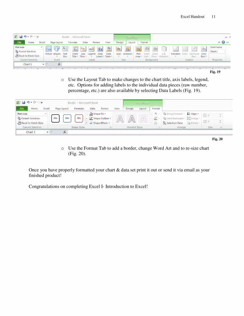
• Under the Chart Tools Tab use the Design, Layout, and Format Tabs to make changes to your graph data.

o Use the Design Tab to change the chart type, color, and to move the chart to

another location or separate tab (Fig. 18).

Fig. 18

Excel Handout 11

Fig. 19

o Use the Layout Tab to make changes to the chart title, axis labels, legend, etc. Options for adding labels to the individual data pieces (raw number, percentage, etc.) are also available by selecting Data Labels (Fig. 19).

o Use the Format Tab to add a border, change Word Art and to re-size chart

(Fig. 20).

Once you have properly formatted your chart & data set print it out or send it via email as your finished product!

Congratulations on completing Excel I- Introduction to Excel!

Fig. 20

Excel Handout 12

Try It!

Scenario: Saving for a house down payment. Need to develop a spreadsheet to track household expenses over the course of a year to figure out how much can be saved each month.

Step One - Data: Rent- 1500 Electric- 70 Water- 15 Telephone- 45 Car Insurance- 100 Cable- 40 Newspaper- 10 Car Payment- 200 Car Repair- 30 Total Expenses- Will Calculate Total Income- 2500

Disposable Income- Will Calculate

Household Budget

Step Two- Formatting & Filling In Data

• Add in Months

• Merge & Center Table Title

• AutoFill numbers across for all months & format number style Step Three- Format Table

• Format Text: Bold Month Names, Right Align, Increase Title Size

• Auto-Fit Column Width

• Add Box Borders to Months & Expenses Step Four- Making Changes

• In April you get a Raise to $2,800.

• In June you cancel the Cable for the rest of the year.

• Calculate Total Expenses & Disposable Income

• Sort Data Alphabetically Step Five- Graph Your Data!

• Create pie chart of January Data

• Change Chart Title to January Expenses

• Move Legend Data to the Left Side Step Six- Print your Results Onto ONE Page

Great Job!! Now you’re ready to take charge of your Excel experience!