Excel 2016 Level 1 – Part II · Excel 2016 Level I, Part 2 Page 6 . Relative versus Absolute Cell Addresses . It is important to understand how Excel identifies cells in formulas

Excel 2016 Level 1 – Part II

Tell Me Assistant New in all Office 2016 applications is the Tell Me Assistant, which is located in the Tell me what you want to do… text box which is located on the top of the ribbon, to the right of the last tab.

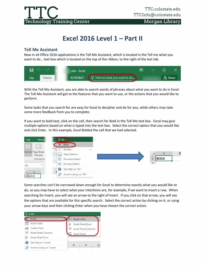
With the Tell Me Assistant, you are able to search words of phrases about what you want to do in Excel. The Tell Me Assistant will get to the features that you want to use, or the actions that you would like to perform. Some tasks that you search for are easy for Excel to decipher and do for you, while others may take some more feedback from you to complete. If you want to bold text, click on the cell, then search for Bold in the Tell Me text box. Excel may give multiple options based on what is typed into the text box. Select the correct option that you would like and click Enter. In this example, Excel Bolded the cell that we had selected.

Some searches can’t be narrowed down enough for Excel to determine exactly what you would like to do, so you may have to select what your intentions are, for example, if we want to Insert a row. When searching for Insert, you will see an arrow to the right of Insert. If you click on that arrow, you will see the options that are available for this specific search. Select the correct action by clicking on it, or using your arrow keys and then clicking Enter when you have chosen the correct action.

© Technology Training Center Colorado State University Excel 2016 Level I, Part 2

Page 2

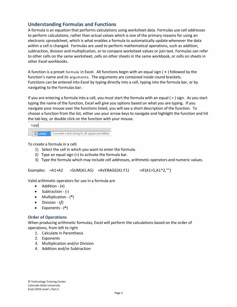
Understanding Formulas and Functions A formula is an equation that performs calculations using worksheet data. Formulas use cell addresses to perform calculations, rather than actual values which is one of the primary reasons for using an electronic spreadsheet, which is what enables a formula to automatically update whenever the data within a cell is changed. Formulas are used to perform mathematical operations, such as addition, subtraction, division and multiplication, or to compare worksheet values or join text. Formulas can refer to other cells on the same worksheet, cells on other sheets in the same workbook, or cells on sheets in other Excel workbooks. A function is a preset formula in Excel. All functions begin with an equal sign ( = ) followed by the function's name and its arguments. The arguments are contained inside round brackets. Functions can be entered into Excel by typing directly into a cell, typing into the formula bar, or by navigating to the Formulas bar. If you are entering a formula into a cell, you must start the formula with an equal ( = ) sign. As you start typing the name of the function, Excel will give you options based on what you are typing. If you navigate your mouse over the functions listed, you will see a short description of the function. To choose a function from the list, either use your arrow keys to navigate and highlight the function and hit the tab key, or double click on the function with your mouse.

To create a formula in a cell; 1) Select the cell in which you want to enter the formula.

2) Type an equal sign (=) to activate the formula bar. 3) Type the formula which may include cell addresses, arithmetic operators and numeric values.

Examples: =A1+A2 =SUM(A1:A5) =AVERAGE(A1:F1) =IF(A1>5,A1*2,””) Valid arithmetic operators for use in a formula are

• Addition - (+) • Subtraction - (-) • Multiplication - (*) • Division - (/) • Exponents - (^)

Order of Operations When producing arithmetic formulas, Excel will perform the calculations based on the order of operations, from left to right

1. Calculate in Parenthesis 2. Exponents 3. Multiplication and/or Division 4. Addition and/or Subtraction


Page 3

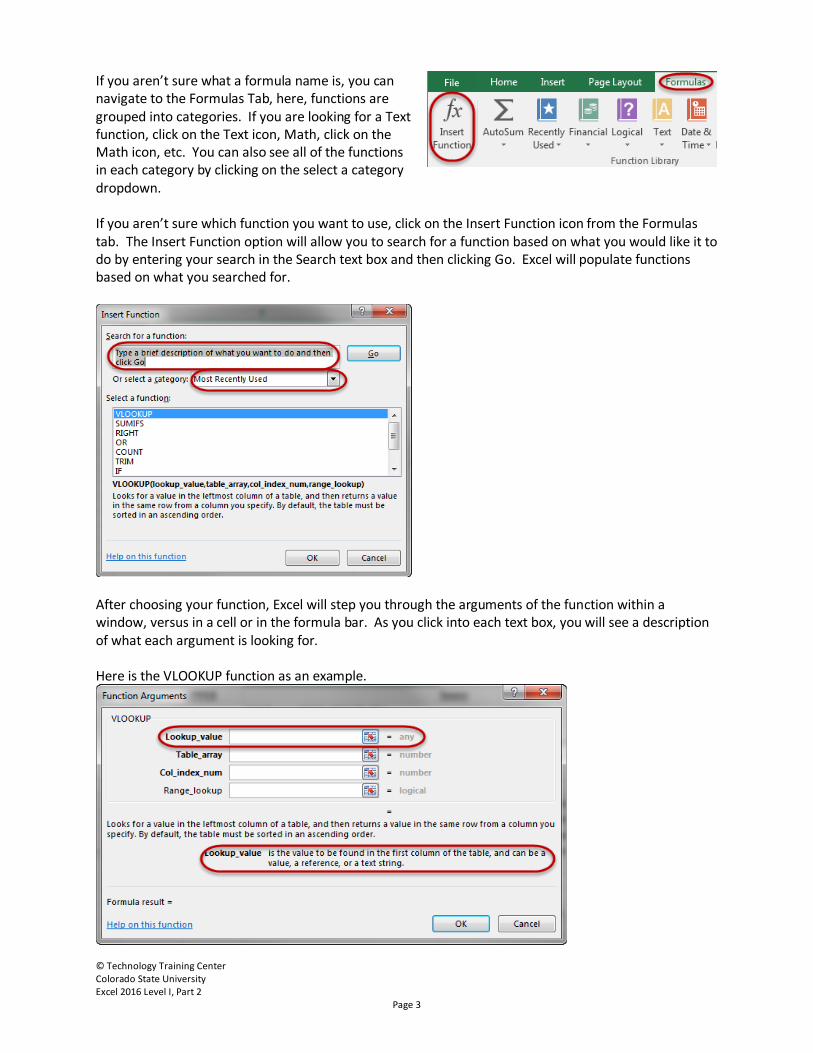
If you aren’t sure what a formula name is, you can navigate to the Formulas Tab, here, functions are grouped into categories. If you are looking for a Text function, click on the Text icon, Math, click on the Math icon, etc. You can also see all of the functions in each category by clicking on the select a category dropdown. If you aren’t sure which function you want to use, click on the Insert Function icon from the Formulas tab. The Insert Function option will allow you to search for a function based on what you would like it to do by entering your search in the Search text box and then clicking Go. Excel will populate functions based on what you searched for.

After choosing your function, Excel will step you through the arguments of the function within a window, versus in a cell or in the formula bar. As you click into each text box, you will see a description of what each argument is looking for. Here is the VLOOKUP function as an example.


Page 4

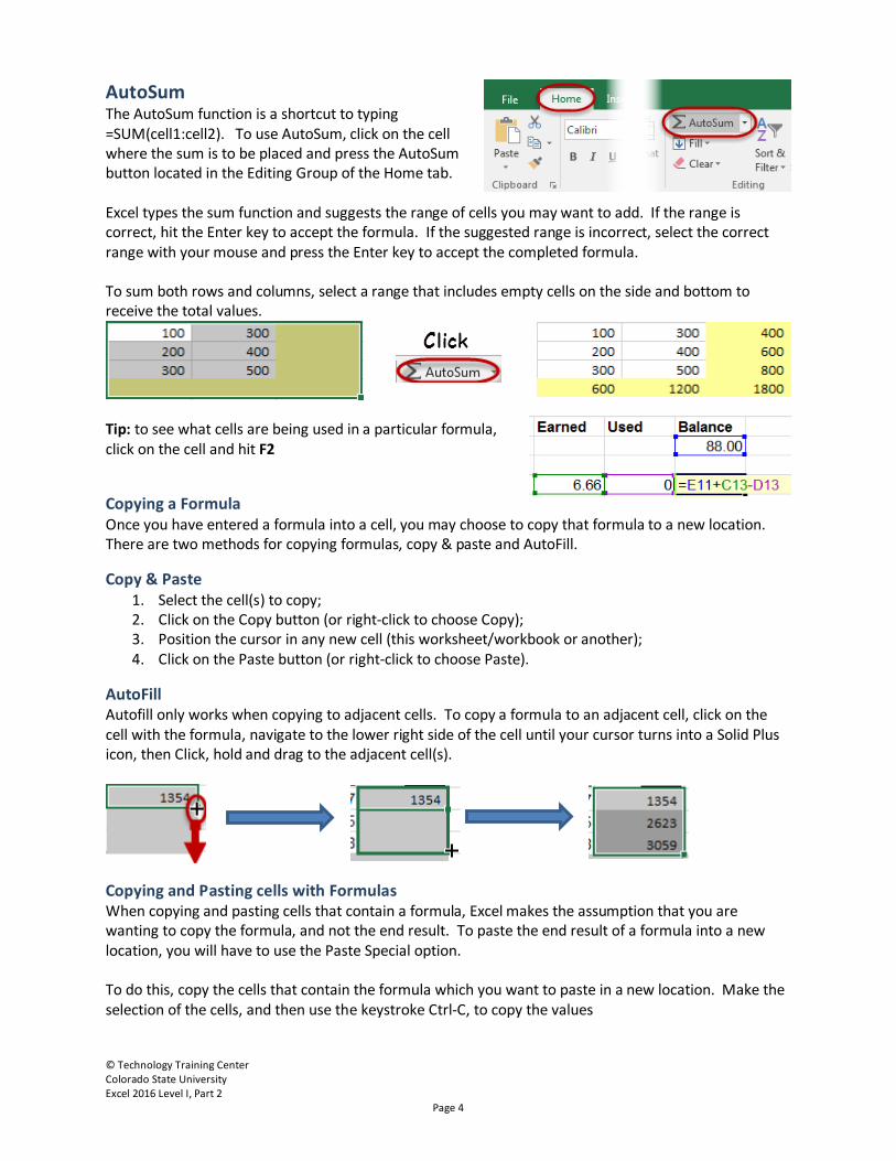
AutoSum The AutoSum function is a shortcut to typing =SUM(cell1:cell2). To use AutoSum, click on the cell where the sum is to be placed and press the AutoSum button located in the Editing Group of the Home tab. Excel types the sum function and suggests the range of cells you may want to add. If the range is correct, hit the Enter key to accept the formula. If the suggested range is incorrect, select the correct range with your mouse and press the Enter key to accept the completed formula. To sum both rows and columns, select a range that includes empty cells on the side and bottom to receive the total values.

Tip: to see what cells are being used in a particular formula, click on the cell and hit F2

Copying a Formula Once you have entered a formula into a cell, you may choose to copy that formula to a new location. There are two methods for copying formulas, copy & paste and AutoFill.

Copy & Paste 1. Select the cell(s) to copy; 2. Click on the Copy button (or right-click to choose Copy); 3. Position the cursor in any new cell (this worksheet/workbook or another); 4. Click on the Paste button (or right-click to choose Paste).

AutoFill Autofill only works when copying to adjacent cells. To copy a formula to an adjacent cell, click on the cell with the formula, navigate to the lower right side of the cell until your cursor turns into a Solid Plus icon, then Click, hold and drag to the adjacent cell(s).

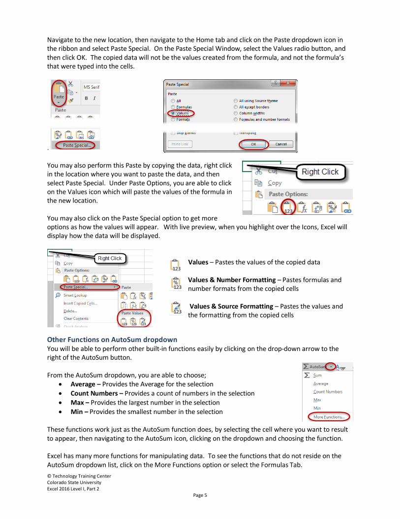
Copying and Pasting cells with Formulas When copying and pasting cells that contain a formula, Excel makes the assumption that you are wanting to copy the formula, and not the end result. To paste the end result of a formula into a new location, you will have to use the Paste Special option. To do this, copy the cells that contain the formula which you want to paste in a new location. Make the selection of the cells, and then use the keystroke Ctrl-C, to copy the values


Page 5

Navigate to the new location, then navigate to the Home tab and click on the Paste dropdown icon in the ribbon and select Paste Special. On the Paste Special Window, select the Values radio button, and then click OK. The copied data will not be the values created from the formula, and not the formula’s that were typed into the cells.

. You may also perform this Paste by copying the data, right click in the location where you want to paste the data, and then select Paste Special. Under Paste Options, you are able to click on the Values icon which will paste the values of the formula in the new location. You may also click on the Paste Special option to get more options as how the values will appear. With live preview, when you highlight over the Icons, Excel will display how the data will be displayed.

Values – Pastes the values of the copied data Values & Number Formatting – Pastes formulas and number formats from the copied cells Values & Source Formatting – Pastes the values and the formatting from the copied cells

Other Functions on AutoSum dropdown You will be able to perform other built-in functions easily by clicking on the drop-down arrow to the right of the AutoSum button. From the AutoSum dropdown, you are able to choose;

• Average – Provides the Average for the selection • Count Numbers – Provides a count of numbers in the selection • Max – Provides the largest number in the selection • Min – Provides the smallest number in the selection

These functions work just as the AutoSum function does, by selecting the cell where you want to result to appear, then navigating to the AutoSum icon, clicking on the dropdown and choosing the function. Excel has many more functions for manipulating data. To see the functions that do not reside on the AutoSum dropdown list, click on the More Functions option or select the Formulas Tab.


Page 6

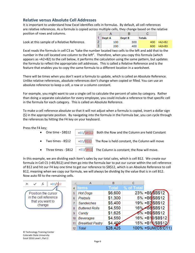
Relative versus Absolute Cell Addresses It is important to understand how Excel identifies cells in formulas. By default, all cell references are relative references. As a formula is copied across multiple cells, they change based on the relative position of rows and columns. Look at this sample of a Relative Reference. Excel reads the formula in cell C3 as “take the number located two cells to the left and add that to the number in the cell located one column to the left”. Therefore, when you copy this formula (which appears as =A2+B2) to the cell below, it performs the calculation using the same pattern, but updates the formula to reflect the appropriate cell addresses. This is called a Relative Reference and is the feature that enables you to copy the same formula to a different location in a worksheet. There will be times when you don’t want a formula to update, which is called an Absolute Reference. Unlike relative references, absolute references don’t change when copied or filled. You can use an absolute reference to keep a cell, a row or a column constant. For example, you might want to use a single cell to calculate the percent of sales by category. Rather than doing a separate calculation for every employee, you could include a reference to that specific cell in the formula for each category. This is called an Absolute Reference. To make a cell reference absolute so that it will not adjust when a formula is copied, insert a dollar sign ($) in the appropriate position. By navigating into the formula in the Formula bar, you can cycle through the references by hitting the F4 key on your keyboard. Press the F4 key;

• One time - $B$12 Both the Row and the Column are held Constant

• Two times - B$12 The Row is held constant, the Column will move

• Three times - $B12 The Column is constant; the Row will move. In this example, we are dividing each item’s sales by our total sales, which is cell B12. We create our formula in Cell C5 (=B5/B12) and then go into the formula bar to put our cursor within the cell reference of B12 and hit our F4 key one time to get our reference to $B$12, which is an Absolute Reference to cell B12, meaning when we copy our formula, we will always be dividing by the value that is in cell B12. Now auto fill to the remaining cells.


Page 7

Sorting When you sort information in a worksheet, you can display the data the way you would like and find specific information quickly. Sorting is done based on columns. You can sort data based on one or more columns of data.

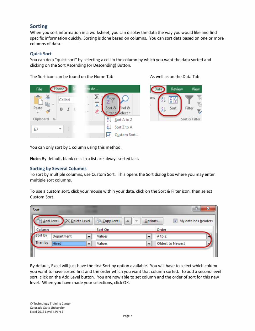
Quick Sort You can do a "quick sort" by selecting a cell in the column by which you want the data sorted and clicking on the Sort Ascending (or Descending) Button. The Sort icon can be found on the Home Tab As well as on the Data Tab

You can only sort by 1 column using this method. Note: By default, blank cells in a list are always sorted last.

Sorting by Several Columns To sort by multiple columns, use Custom Sort. This opens the Sort dialog box where you may enter multiple sort columns. To use a custom sort, click your mouse within your data, click on the Sort & Filter icon, then select Custom Sort.

By default, Excel will just have the first Sort by option available. You will have to select which column you want to have sorted first and the order which you want that column sorted. To add a second level sort, click on the Add Level button. You are now able to set column and the order of sort for this new level. When you have made your selections, click OK.


Page 8

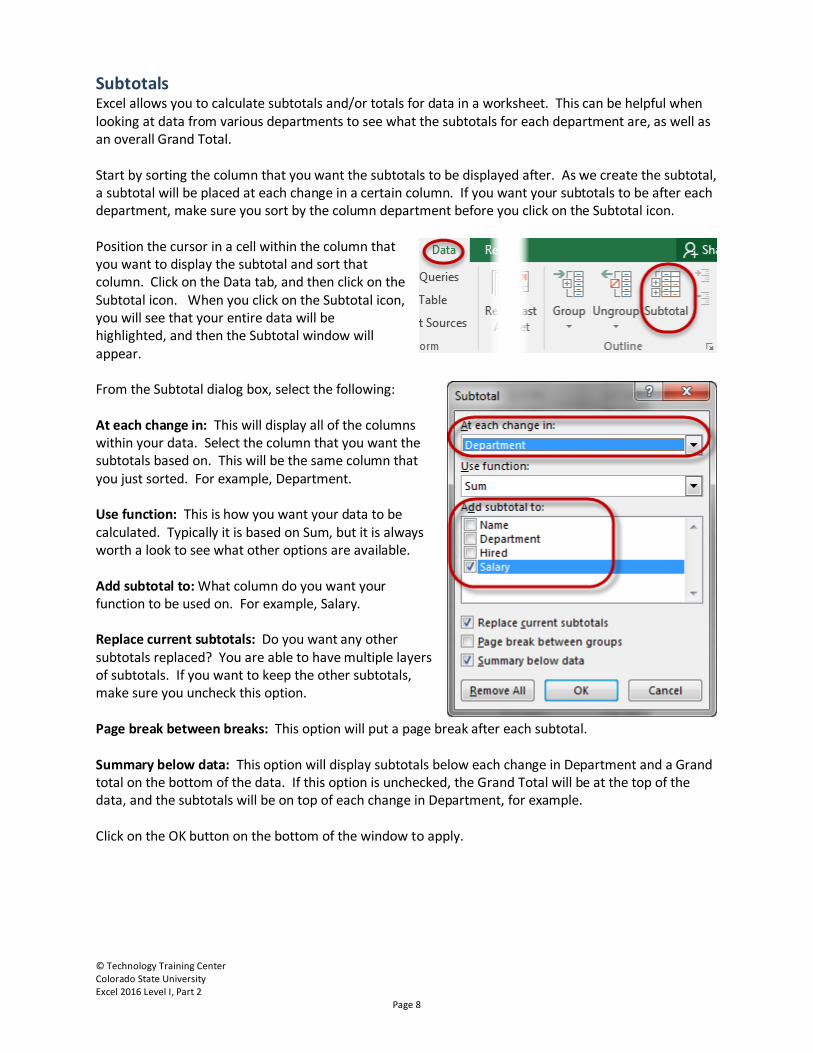
Subtotals Excel allows you to calculate subtotals and/or totals for data in a worksheet. This can be helpful when looking at data from various departments to see what the subtotals for each department are, as well as an overall Grand Total. Start by sorting the column that you want the subtotals to be displayed after. As we create the subtotal, a subtotal will be placed at each change in a certain column. If you want your subtotals to be after each department, make sure you sort by the column department before you click on the Subtotal icon. Position the cursor in a cell within the column that you want to display the subtotal and sort that column. Click on the Data tab, and then click on the Subtotal icon. When you click on the Subtotal icon, you will see that your entire data will be highlighted, and then the Subtotal window will appear. From the Subtotal dialog box, select the following: At each change in: This will display all of the columns within your data. Select the column that you want the subtotals based on. This will be the same column that you just sorted. For example, Department. Use function: This is how you want your data to be calculated. Typically it is based on Sum, but it is always worth a look to see what other options are available. Add subtotal to: What column do you want your function to be used on. For example, Salary. Replace current subtotals: Do you want any other subtotals replaced? You are able to have multiple layers of subtotals. If you want to keep the other subtotals, make sure you uncheck this option. Page break between breaks: This option will put a page break after each subtotal. Summary below data: This option will display subtotals below each change in Department and a Grand total on the bottom of the data. If this option is unchecked, the Grand Total will be at the top of the data, and the subtotals will be on top of each change in Department, for example. Click on the OK button on the bottom of the window to apply.


Page 9

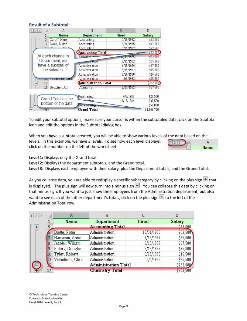
Result of a Subtotal:

To edit your subtotal options, make sure your cursor is within the subtotaled data, click on the Subtotal icon and edit the options in the Subtotal dialog box. When you have a subtotal created, you will be able to show various levels of the data based on the levels. In this example, we have 3 levels. To see how each level displays, click on the number on the left of the worksheet. Level 1: Displays only the Grand total. Level 2: Displays the department subtotals, and the Grand total. Level 3: Displays each employee with their salary, plus the Department totals, and the Grand Total. As you collapse data, you are able to redisplay a specific subcategory by clicking on the plus sign that is displayed. The plus sign will now turn into a minus sign . You can collapse this data by clicking on that minus sign. If you want to just show the employees from the Administration department, but also want to see each of the other department’s totals, click on the plus sign to the left of the Administration Total row.


Page 10

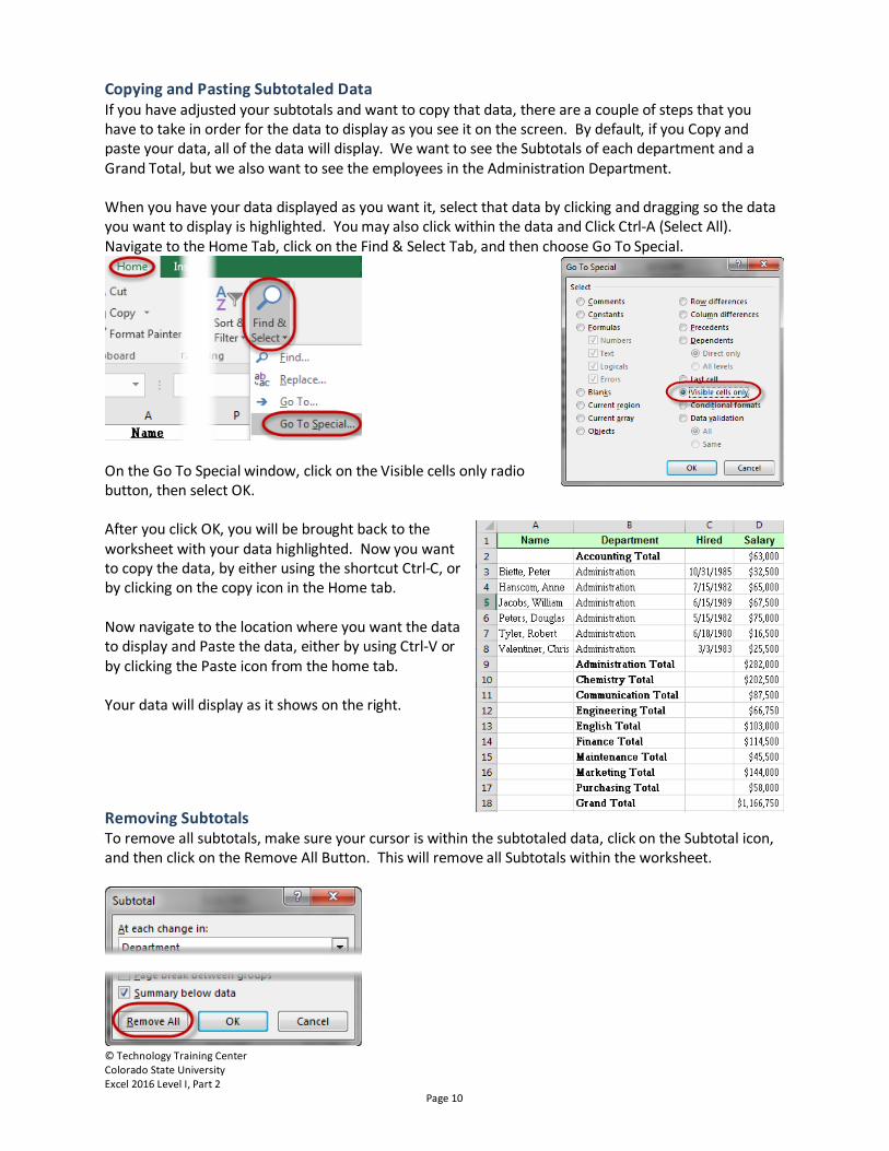
Copying and Pasting Subtotaled Data If you have adjusted your subtotals and want to copy that data, there are a couple of steps that you have to take in order for the data to display as you see it on the screen. By default, if you Copy and paste your data, all of the data will display. We want to see the Subtotals of each department and a Grand Total, but we also want to see the employees in the Administration Department. When you have your data displayed as you want it, select that data by clicking and dragging so the data you want to display is highlighted. You may also click within the data and Click Ctrl-A (Select All). Navigate to the Home Tab, click on the Find & Select Tab, and then choose Go To Special.

On the Go To Special window, click on the Visible cells only radio button, then select OK. After you click OK, you will be brought back to the worksheet with your data highlighted. Now you want to copy the data, by either using the shortcut Ctrl-C, or by clicking on the copy icon in the Home tab. Now navigate to the location where you want the data to display and Paste the data, either by using Ctrl-V or by clicking the Paste icon from the home tab. Your data will display as it shows on the right.

Removing Subtotals To remove all subtotals, make sure your cursor is within the subtotaled data, click on the Subtotal icon, and then click on the Remove All Button. This will remove all Subtotals within the worksheet.


Page 11

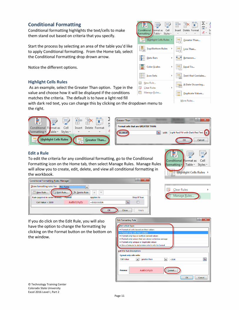
Conditional Formatting Conditional formatting highlights the text/cells to make them stand out based on criteria that you specify. Start the process by selecting an area of the table you’d like to apply Conditional formatting. From the Home tab, select the Conditional Formatting drop drown arrow. Notice the different options.

Highlight Cells Rules As an example, select the Greater Than option. Type in the value and choose how it will be displayed if the conditions matches the criteria. The default is to have a light red fill with dark red text, you can change this by clicking on the dropdown menu to the right.

Edit a Rule To edit the criteria for any conditional formatting, go to the Conditional Formatting icon on the Home tab, then select Manage Rules. Manage Rules will allow you to create, edit, delete, and view all conditional formatting in the workbook.

If you do click on the Edit Rule, you will also have the option to change the formatting by clicking on the Format button on the bottom on the window.


Page 12

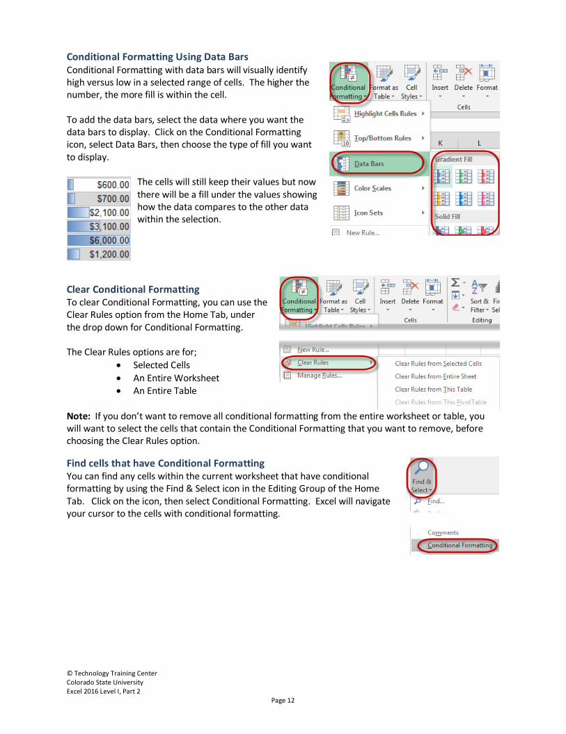
Conditional Formatting Using Data Bars Conditional Formatting with data bars will visually identify high versus low in a selected range of cells. The higher the number, the more fill is within the cell. To add the data bars, select the data where you want the data bars to display. Click on the Conditional Formatting icon, select Data Bars, then choose the type of fill you want to display.

The cells will still keep their values but now there will be a fill under the values showing how the data compares to the other data within the selection.

Clear Conditional Formatting To clear Conditional Formatting, you can use the Clear Rules option from the Home Tab, under the drop down for Conditional Formatting. The Clear Rules options are for;

• Selected Cells • An Entire Worksheet • An Entire Table

Note: If you don’t want to remove all conditional formatting from the entire worksheet or table, you will want to select the cells that contain the Conditional Formatting that you want to remove, before choosing the Clear Rules option.

Find cells that have Conditional Formatting You can find any cells within the current worksheet that have conditional formatting by using the Find & Select icon in the Editing Group of the Home Tab. Click on the icon, then select Conditional Formatting. Excel will navigate your cursor to the cells with conditional formatting.


Page 13

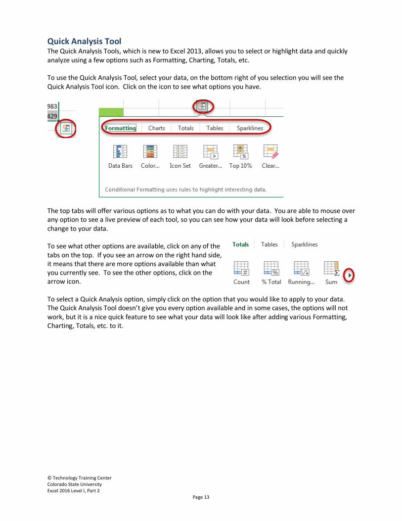
Quick Analysis Tool The Quick Analysis Tools, which is new to Excel 2013, allows you to select or highlight data and quickly analyze using a few options such as Formatting, Charting, Totals, etc. To use the Quick Analysis Tool, select your data, on the bottom right of you selection you will see the Quick Analysis Tool icon. Click on the icon to see what options you have.

The top tabs will offer various options as to what you can do with your data. You are able to mouse over any option to see a live preview of each tool, so you can see how your data will look before selecting a change to your data. To see what other options are available, click on any of the tabs on the top. If you see an arrow on the right hand side, it means that there are more options available than what you currently see. To see the other options, click on the arrow icon. To select a Quick Analysis option, simply click on the option that you would like to apply to your data. The Quick Analysis Tool doesn’t give you every option available and in some cases, the options will not work, but it is a nice quick feature to see what your data will look like after adding various Formatting, Charting, Totals, etc. to it.


Page 14

Converting Text to Columns There will be times when you have data in one column that really should be broken down to two columns. For example, if you have a spreadsheet with the first and last name in one column and you want to divide the data into two columns. Tip: Make sure you have enough blank columns to get your new data placed in. You may have to insert a couple columns in order to make this happen. Select the text to be divided and navigate to the Data tab, Data Tools Group. Select the Text to Columns icon and follow the wizard to divide your data from one column to two. Step 1: Excel will examine the data and determine what type of data you have. Typically this is correct, but always check to make sure your data is either Delimited (has a comma, tab, etc. separating the data) or Fixed width (a specific amount of space separating the text) Click Next Step 2: Choose the separator for the data. In my example, the comma is the separator. As you click through the options, you will see how the data will be effected. You want to have a solid line between the pieces of data that you are trying to separate.


Page 15

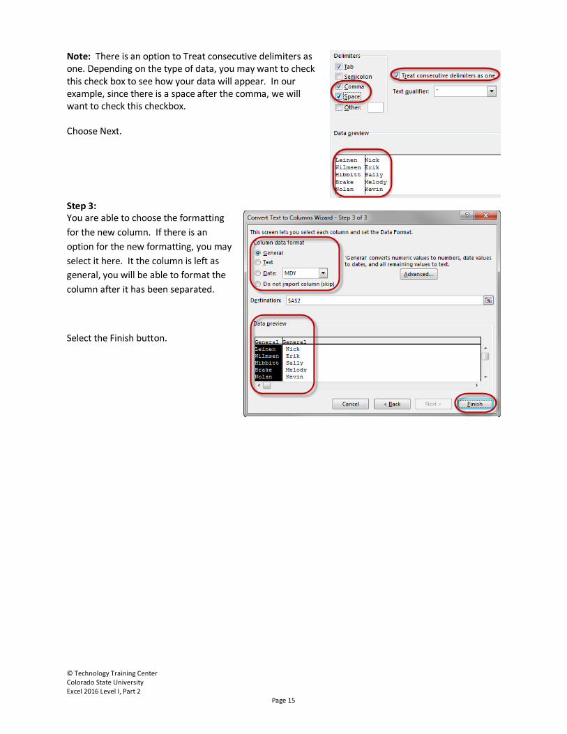
Note: There is an option to Treat consecutive delimiters as one. Depending on the type of data, you may want to check this check box to see how your data will appear. In our example, since there is a space after the comma, we will want to check this checkbox. Choose Next. Step 3: You are able to choose the formatting for the new column. If there is an option for the new formatting, you may select it here. It the column is left as general, you will be able to format the column after it has been separated.

Select the Finish button.


Page 16

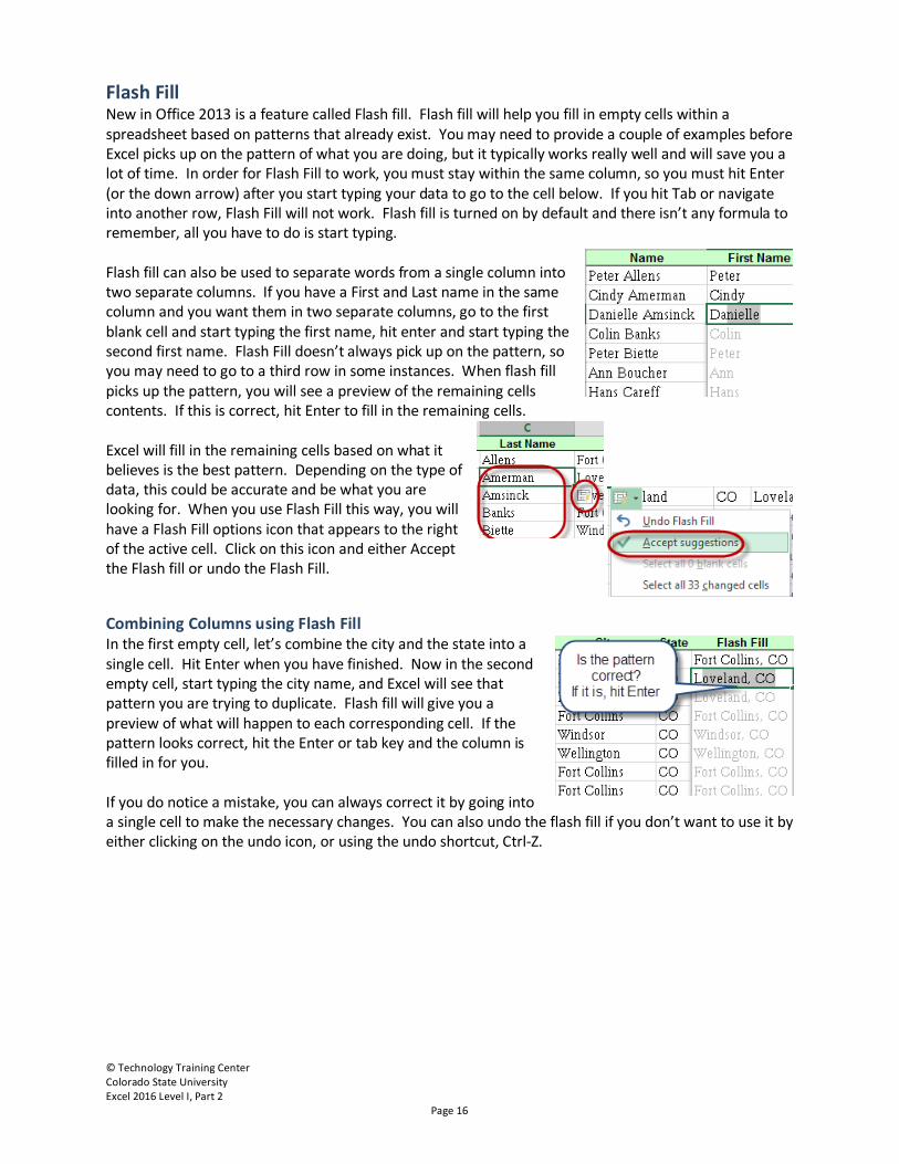
Flash Fill New in Office 2013 is a feature called Flash fill. Flash fill will help you fill in empty cells within a spreadsheet based on patterns that already exist. You may need to provide a couple of examples before Excel picks up on the pattern of what you are doing, but it typically works really well and will save you a lot of time. In order for Flash Fill to work, you must stay within the same column, so you must hit Enter (or the down arrow) after you start typing your data to go to the cell below. If you hit Tab or navigate into another row, Flash Fill will not work. Flash fill is turned on by default and there isn’t any formula to remember, all you have to do is start typing. Flash fill can also be used to separate words from a single column into two separate columns. If you have a First and Last name in the same column and you want them in two separate columns, go to the first blank cell and start typing the first name, hit enter and start typing the second first name. Flash Fill doesn’t always pick up on the pattern, so you may need to go to a third row in some instances. When flash fill picks up the pattern, you will see a preview of the remaining cells contents. If this is correct, hit Enter to fill in the remaining cells. Excel will fill in the remaining cells based on what it believes is the best pattern. Depending on the type of data, this could be accurate and be what you are looking for. When you use Flash Fill this way, you will have a Flash Fill options icon that appears to the right of the active cell. Click on this icon and either Accept the Flash fill or undo the Flash Fill.

Combining Columns using Flash Fill In the first empty cell, let’s combine the city and the state into a single cell. Hit Enter when you have finished. Now in the second empty cell, start typing the city name, and Excel will see that pattern you are trying to duplicate. Flash fill will give you a preview of what will happen to each corresponding cell. If the pattern looks correct, hit the Enter or tab key and the column is filled in for you. If you do notice a mistake, you can always correct it by going into a single cell to make the necessary changes. You can also undo the flash fill if you don’t want to use it by either clicking on the undo icon, or using the undo shortcut, Ctrl-Z.


Page 17

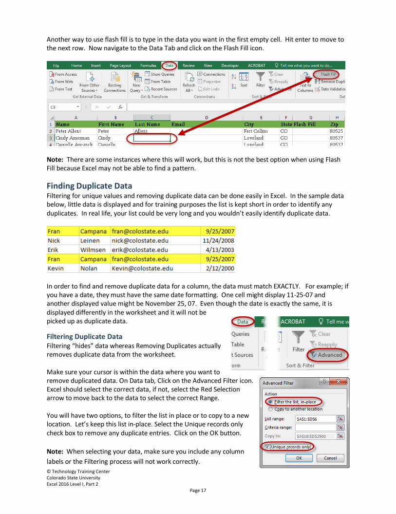
Another way to use flash fill is to type in the data you want in the first empty cell. Hit enter to move to the next row. Now navigate to the Data Tab and click on the Flash Fill icon.

Note: There are some instances where this will work, but this is not the best option when using Flash Fill because Excel may not be able to find a pattern.

Finding Duplicate Data Filtering for unique values and removing duplicate data can be done easily in Excel. In the sample data below, little data is displayed and for training purposes the list is kept short in order to identify any duplicates. In real life, your list could be very long and you wouldn’t easily identify duplicate data.

In order to find and remove duplicate data for a column, the data must match EXACTLY. For example; if you have a date, they must have the same date formatting. One cell might display 11-25-07 and another displayed value might be November 25, 07. Even though the date is exactly the same, it is displayed differently in the worksheet and it will not be picked up as duplicate data.

Filtering Duplicate Data Filtering “hides” data whereas Removing Duplicates actually removes duplicate data from the worksheet. Make sure your cursor is within the data where you want to remove duplicated data. On Data tab, Click on the Advanced Filter icon. Excel should select the correct data, if not, select the Red Selection arrow to move back to the data to select the correct Range. You will have two options, to filter the list in place or to copy to a new location. Let’s keep this list in-place. Select the Unique records only check box to remove any duplicate entries. Click on the OK button. Note: When selecting your data, make sure you include any column labels or the Filtering process will not work correctly.


Page 18

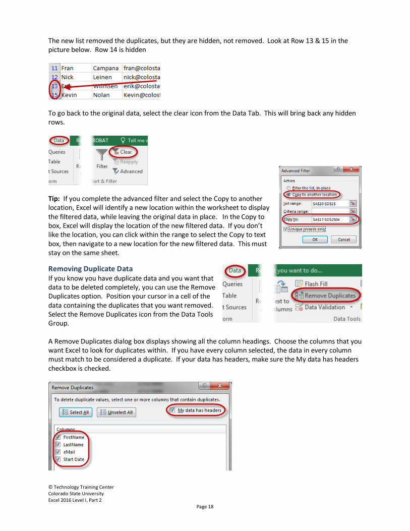
The new list removed the duplicates, but they are hidden, not removed. Look at Row 13 & 15 in the picture below. Row 14 is hidden

To go back to the original data, select the clear icon from the Data Tab. This will bring back any hidden rows.

Tip: If you complete the advanced filter and select the Copy to another location, Excel will identify a new location within the worksheet to display the filtered data, while leaving the original data in place. In the Copy to box, Excel will display the location of the new filtered data. If you don’t like the location, you can click within the range to select the Copy to text box, then navigate to a new location for the new filtered data. This must stay on the same sheet.

Removing Duplicate Data If you know you have duplicate data and you want that data to be deleted completely, you can use the Remove Duplicates option. Position your cursor in a cell of the data containing the duplicates that you want removed. Select the Remove Duplicates icon from the Data Tools Group. A Remove Duplicates dialog box displays showing all the column headings. Choose the columns that you want Excel to look for duplicates within. If you have every column selected, the data in every column must match to be considered a duplicate. If your data has headers, make sure the My data has headers checkbox is checked.


Page 19

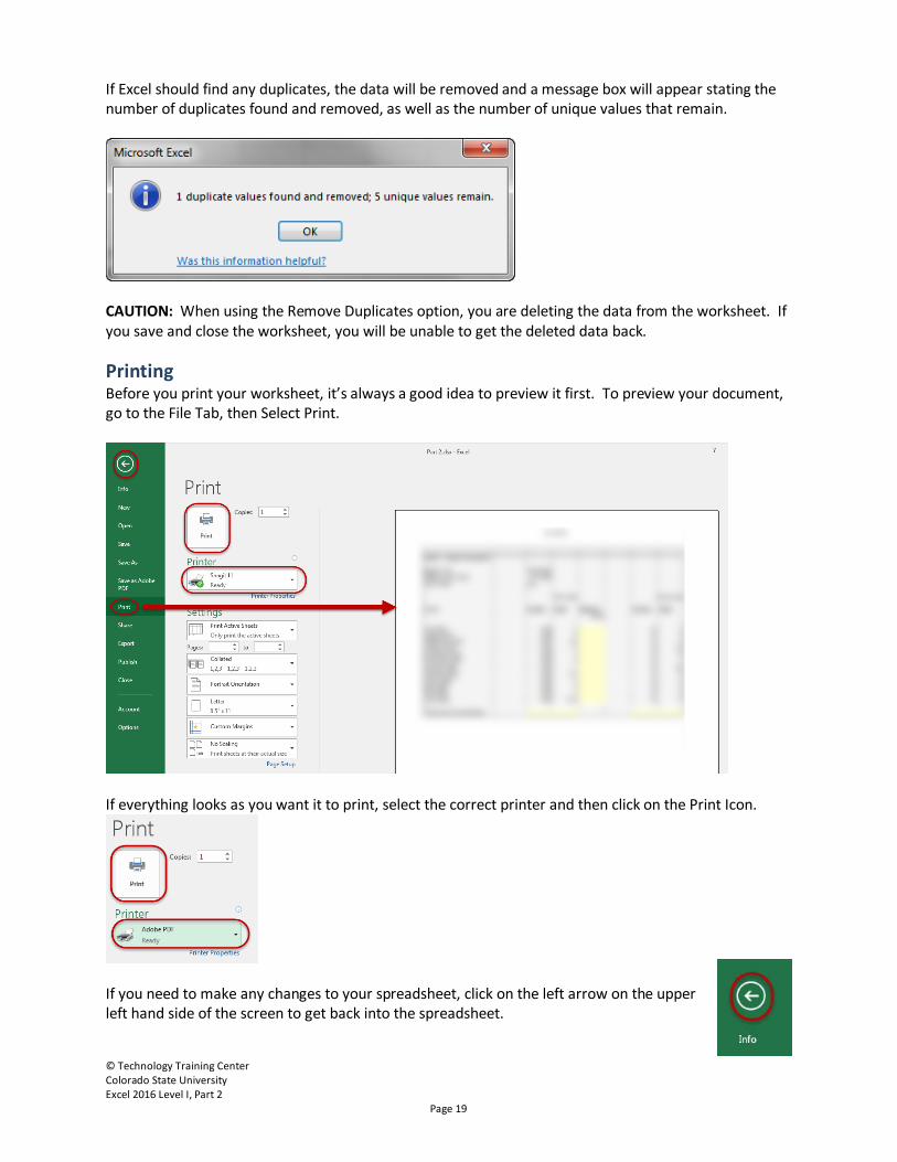
If Excel should find any duplicates, the data will be removed and a message box will appear stating the number of duplicates found and removed, as well as the number of unique values that remain.

CAUTION: When using the Remove Duplicates option, you are deleting the data from the worksheet. If you save and close the worksheet, you will be unable to get the deleted data back.

Printing Before you print your worksheet, it’s always a good idea to preview it first. To preview your document, go to the File Tab, then Select Print.

If everything looks as you want it to print, select the correct printer and then click on the Print Icon.

If you need to make any changes to your spreadsheet, click on the left arrow on the upper left hand side of the screen to get back into the spreadsheet.


Page 20

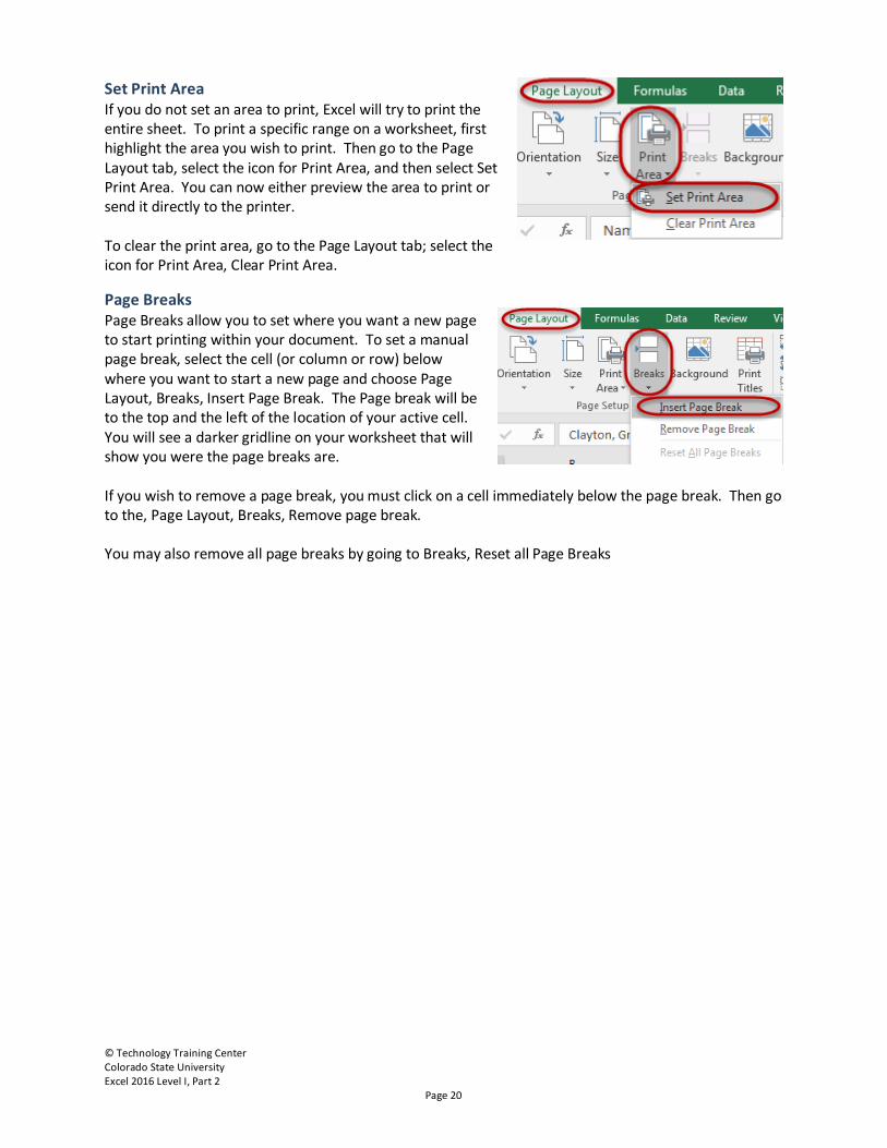
Set Print Area If you do not set an area to print, Excel will try to print the entire sheet. To print a specific range on a worksheet, first highlight the area you wish to print. Then go to the Page Layout tab, select the icon for Print Area, and then select Set Print Area. You can now either preview the area to print or send it directly to the printer. To clear the print area, go to the Page Layout tab; select the icon for Print Area, Clear Print Area.

Page Breaks Page Breaks allow you to set where you want a new page to start printing within your document. To set a manual page break, select the cell (or column or row) below where you want to start a new page and choose Page Layout, Breaks, Insert Page Break. The Page break will be to the top and the left of the location of your active cell. You will see a darker gridline on your worksheet that will show you were the page breaks are. If you wish to remove a page break, you must click on a cell immediately below the page break. Then go to the, Page Layout, Breaks, Remove page break. You may also remove all page breaks by going to Breaks, Reset all Page Breaks


Page 21

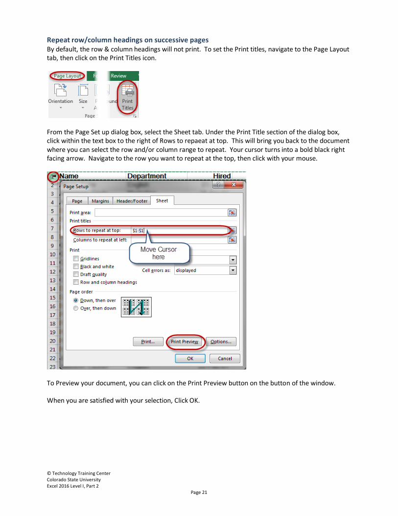
Repeat row/column headings on successive pages By default, the row & column headings will not print. To set the Print titles, navigate to the Page Layout tab, then click on the Print Titles icon.

From the Page Set up dialog box, select the Sheet tab. Under the Print Title section of the dialog box, click within the text box to the right of Rows to repaeat at top. This will bring you back to the document where you can select the row and/or column range to repeat. Your cursor turns into a bold black right facing arrow. Navigate to the row you want to repeat at the top, then click with your mouse.

To Preview your document, you can click on the Print Preview button on the button of the window. When you are satisfied with your selection, Click OK.


Page 22

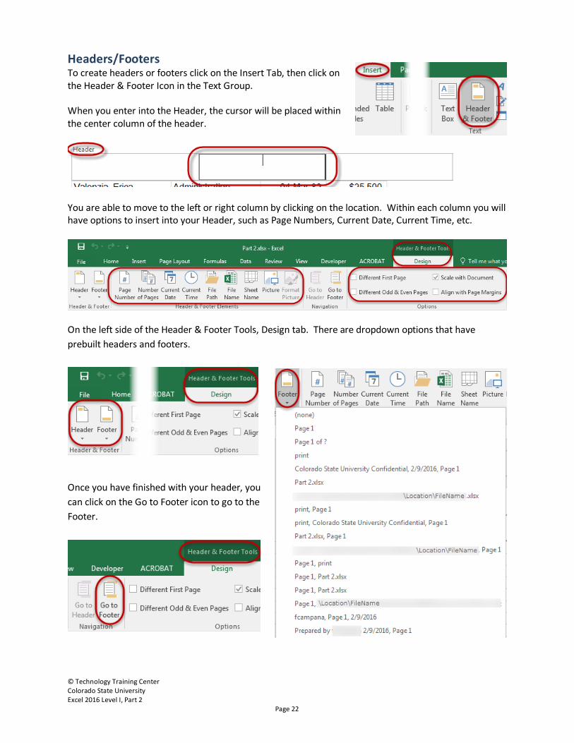
Headers/Footers To create headers or footers click on the Insert Tab, then click on the Header & Footer Icon in the Text Group. When you enter into the Header, the cursor will be placed within the center column of the header.

You are able to move to the left or right column by clicking on the location. Within each column you will have options to insert into your Header, such as Page Numbers, Current Date, Current Time, etc.

On the left side of the Header & Footer Tools, Design tab. There are dropdown options that have prebuilt headers and footers.

Once you have finished with your header, you can click on the Go to Footer icon to go to the Footer.


Page 23

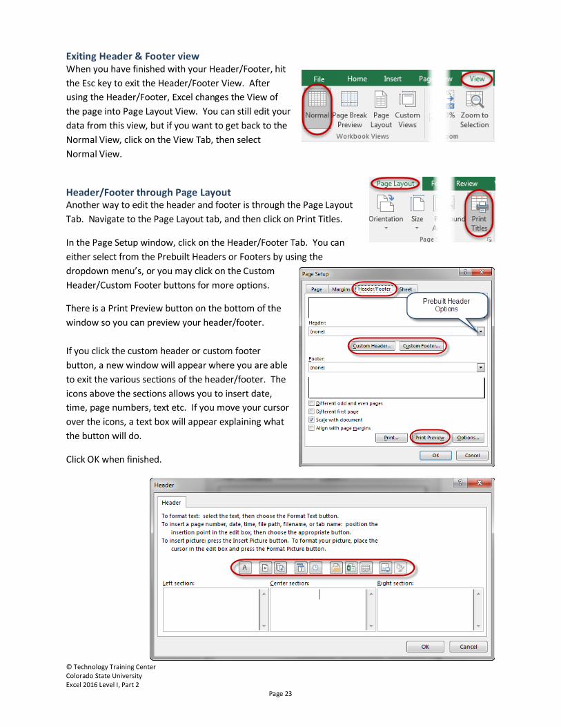
Exiting Header & Footer view When you have finished with your Header/Footer, hit the Esc key to exit the Header/Footer View. After using the Header/Footer, Excel changes the View of the page into Page Layout View. You can still edit your data from this view, but if you want to get back to the Normal View, click on the View Tab, then select Normal View.

Header/Footer through Page Layout Another way to edit the header and footer is through the Page Layout Tab. Navigate to the Page Layout tab, and then click on Print Titles.

In the Page Setup window, click on the Header/Footer Tab. You can either select from the Prebuilt Headers or Footers by using the dropdown menu’s, or you may click on the Custom Header/Custom Footer buttons for more options.

There is a Print Preview button on the bottom of the window so you can preview your header/footer. If you click the custom header or custom footer button, a new window will appear where you are able to exit the various sections of the header/footer. The icons above the sections allows you to insert date, time, page numbers, text etc. If you move your cursor over the icons, a text box will appear explaining what the button will do.

Click OK when finished.

Documents

Excel 2016 Level 1 – Part II · Excel 2016 Level I, Part 2 Page 6 . Relative versus Absolute Cell Addresses . It is important to understand how Excel identifies cells in formulas