More Excel 2007 Formulas - Maxwell School of …More Excel 2007 Formulas Training Session Handout Page 2 Topics came directly from Microsoft Excel Help. Overview A formula is a sequence

More Excel 2007 Formulas Training Session Handout Page 1

Topics came directly from Microsoft Excel Help.

More Excel 2007 Formulas Table of Contents

OVERVIEW ...................................................................................................................................................................... 2 CALCULATION OPERATORS AND PRECEDENCE .............................................................................................. 2

TYPES OF OPERATORS ....................................................................................................................................................... 2

Arithmetic operators .................................................................................................................................................... 2 Comparison operators .................................................................................................................................................. 3 Text concatenation operator ........................................................................................................................................ 3 Reference operators ..................................................................................................................................................... 3

THE ORDER IN WHICH EXCEL PERFORMS OPERATIONS IN FORMULAS ................................................................................ 3

Calculation order ......................................................................................................................................................... 3 Operator precedence .................................................................................................................................................... 3

THE DIFFERENCE BETWEEN ABSOLUTE, RELATIVE AND MIXED REFERENCES .................................. 4 RELATIVE REFERENCES .................................................................................................................................................... 4 ABSOLUTE REFERENCES ................................................................................................................................................... 4 MIXED REFERENCES ......................................................................................................................................................... 4

DEFINE AND USE NAMES IN FORMULAS .............................................................................................................. 5 THE SCOPE OF A NAME ...................................................................................................................................................... 5 DEFINING AND ENTERING NAMES ..................................................................................................................................... 6

LEARN ABOUT SYNTAX RULES FOR NAMES ....................................................................................................................... 6 DEFINE A NAME FOR A CELL OR CELL RANGE ON A WORKSHEET ....................................................................................... 6

DEFINE A NAME BY USING A SELECTION OF CELLS IN THE WORKSHEET ............................................................................ 7 DEFINE A NAME BY USING THE NEW NAME DIALOG BOX.................................................................................................. 7 MANAGE NAMES BY USING THE NAME MANAGER DIALOG BOX ....................................................................................... 7

VIEW NAMES .................................................................................................................................................................... 8

CHANGE A NAME .............................................................................................................................................................. 9 DELETE ONE OR MORE NAMES .......................................................................................................................................... 9

CREATE FORMULAS .................................................................................................................................................... 9 CREATE A SIMPLE FORMULA BY USING CONSTANTS AND CALCULATION OPERATORS ....................................................... 9 CREATE A FORMULA BY USING CELL REFERENCES AND NAMES ........................................................................................ 9

CREATE A FORMULA BY USING A FUNCTION ................................................................................................................... 10 DELETE A FORMULA ....................................................................................................................................................... 10

IF FUNCTION ................................................................................................................................................................ 11 SYNTAX .......................................................................................................................................................................... 11

SUMIF FUNCTION ....................................................................................................................................................... 13 SYNTAX .......................................................................................................................................................................... 13

SUMIFS FUNCTION ..................................................................................................................................................... 15 SYNTAX .......................................................................................................................................................................... 15

VLOOKUP FUNCTION ................................................................................................................................................ 17 SYNTAX .......................................................................................................................................................................... 18

Example 1 .................................................................................................................................................................. 19 Example 2 .................................................................................................................................................................. 20

HLOOKUP FUNCTION ................................................................................................................................................ 21 SYNTAX .......................................................................................................................................................................... 21

Example ..................................................................................................................................................................... 22

AVOID COMMON ERRORS WHEN CREATING FORMULAS ........................................................................... 22



Overview A formula is a sequence of values, cell references, names, functions, or operators in a cell that together

produce a new value. Formulas are equations that perform calculations on values in your worksheet. A

formula always starts with an equal sign (=).

You can create a simple formula by using constants and calculation operators. A constant is a value that is

not calculated. For example, the number 210 and the text "Quarterly Earnings" are constants. An operator is a

sign or symbol that specifies the type of calculation to perform within an expression. There are mathematical,

comparison, logical, and reference operators. An expression, or a value resulting from an expression, is not a

constant.

You can also create a formula by using a function. A function is a prewritten formula that takes a value or

values, performs an operation, and returns a value or values. Use functions to simplify and shorten formulas

on a worksheet, especially those that perform lengthy or complex calculations.

Depending on the type of formula that you create, a formula can contain any or all of the following parts.

Functions: A function starts with an equal sign (=), and you can enter arguments for the function within its

parentheses. Each function has a specific argument syntax.

Cell references: You can refer to data in worksheet cells by including cell references in the formula. For

example, the cell reference A2 returns the value of that cell or uses that value in the calculation.

Constants: You can also enter constants, such as numbers or text values, directly into a formula.

Operators: Operators are the symbols that are used to specify the type of calculation that you want the

formula to perform. For example, the ^ (caret) operator raises a number to a power, and the * (asterisk)

operator multiplies numbers.

To achieve the calculation result that you want, you can use a single function or nested functions that calculate

single or multiple results. You can delete any formula when it's no longer needed.

Calculation operators and precedence Operators specify the type of calculation that you want to perform on the elements of a formula. There is a

default order in which calculations occur, but you can change this order by using parentheses.

Types of operators There are four different types of calculation operators: arithmetic, comparison, text concatenation, and

reference.

Arithmetic operators To perform basic mathematical operations such as addition, subtraction, or multiplication;

combine numbers; and produce numeric results, use the following arithmetic operators.

Arithmetic

operator Meaning Example

Arithmetic

operator Meaning Example

+ (plus sign) Addition 3+3 / (forward slash) Division 3/3

– (minus sign) Subtraction

Negation

3–1

–1

% (percent sign) Percent 20%

* (asterisk) Multiplication 3*3 ^ (caret) Exponentiation 3^2



Comparison operators You can compare two values with the following operators. When two values are compared

by using these operators, the result is a logical value either TRUE or FALSE.

Comparison

operator

Meaning Example Comparison

operator

Meaning Example

= equal sign

Equal to A1=B1 >=

greater than or equal

to sign

Greater than or

equal to

A1>=B1

>

greater than

sign

Greater than A1>B1 <= less than or equal to

sign

Less than or

equal to

A1<=B1

< less than sign

Less than A1<B1 <>

not equal to sign

Not equal to A1<>B1

Text concatenation operator Use the ampersand (&) to join, or concatenate, one or more text strings to produce a single piece of text.

Text operator Meaning Example

& (ampersand) Connects, or concatenates, two values to produce one

continuous text value

("North"&"wind")

Reference operators Combine ranges of cells for calculations with the following operators.

Reference

operator

Meaning Example

: (colon) Range operator, which produces one reference to all the cells

between two references, including the two references

B5:B15

, (comma) Union operator, which combines multiple references into one

reference

SUM(B5:B15,D5:D15)

The order in which Excel performs operations in formulas In some cases, the order in which a calculation is performed can affect the return value of the formula, so it's

important to understand how the order is determined and how you can change the order to obtain desired

results.

Calculation order Formulas calculate values in a specific order. A formula in Excel always begins with an equal sign (=). The

equal sign tells Excel that the succeeding characters constitute a formula. Following the equal sign are the

elements to be calculated (the operands), which are separated by calculation operators. Excel calculates the

formula from left to right, according to a specific order for each operator in the formula.

Operator precedence If you combine several operators in a single formula, Excel performs the operations in the order shown on the

next page. If a formula contains operators with the same precedence — for example, if a formula contains

both a multiplication and division operator — Excel evaluates the operators from left to right.



To keep things simple, the ―Order of Operations‖ in a basic Excel formula is as follows:

1) Parenthesis

2) Exponents

3) Multiplication or Division – if both operators appear in the same formula, Excel evaluates the operators

from left to right.

4) Addition or Subtraction – if both operators appear in the same formula, Excel evaluates the operators

from left to right.

Tip: To recall the order of operations, try remembering:

Please Excuse My Dear Aunt Sally.

To change the order of evaluation, enclose in parentheses the part of the formula to be calculated first.

Example, the following formula produces 11 because Excel calculates multiplication

before addition. The formula multiplies 2 by 3 and then adds 5 to the result. =5+2*3

In contrast, if you use parentheses to change the syntax, Excel adds 5 and 2 together

and then multiplies the result by 3 to produce 21.

=(5+2)*3

The difference between absolute, relative and mixed references

Relative references: A relative cell reference in a formula, such as A1, is based on the relative position

of the cell that contains the formula and the cell the reference refers to. If the position of the cell that contains

the formula changes, the reference is changed. If you copy or fill the formula across rows or down columns,

the reference automatically adjusts. By default, new formulas use relative references. For example, if you

copy or fill a relative reference in cell B2 to cell B3, it automatically adjusts from =A1 to =A2.

Copied formula with

relative reference

Absolute references: An absolute cell reference in a formula, such as $A$1, always refers to a cell in a

specific location. If the position of the cell that contains the formula changes, the absolute reference remains

the same. If you copy or fill the formula across rows or down columns, the absolute reference does not adjust.

By default, new formulas use relative references, and you may need to switch them to absolute references. For

example, if you copy or fill an absolute reference in cell B2 to cell B3, it stays the same in both cells =$A$1.

Copied formula with

absolute reference

Mixed references: A mixed reference has either an absolute column and relative row, or absolute row

and relative column. An absolute column reference takes the form $A1, $B1, and so on. An absolute row

reference takes the form A$1, B$1, and so on. If the position of the cell that contains the formula changes, the

relative reference is changed, and the absolute reference does not change. If you copy or fill the formula

across rows or down columns, the relative reference automatically adjusts, and the absolute reference does not

adjust. For example, if you copy or fill a mixed reference from cell A2 to B3, it adjusts from =A$1 to =B$1.

Copied formula with

mixed reference



Define and use names in formulas By using names (a word or string of characters in Excel that represents a cell, range of cells, formula, or

constant value), you can make your formulas much easier to understand and maintain. You can define a name

for a cell range, function, constant, or table. Once you adopt the practice of using names in your workbook,

you can easily update, audit, and manage these names.

A name is a meaningful shorthand that makes it easier to understand the purpose of a cell reference, constant,

formula, or table, each of which may be difficult to comprehend at first glance. You can create your own

defined name, and Microsoft Office Excel sometimes creates a defined name for you, such as when you set a

print area. The following information shows common examples of names and how they can improve clarity

and understanding.

Example Type Example with no name Example with a name

Reference =SUM(C20:C30) =SUM(FirstQuarterSales)

Constant =PRODUCT(A5,8.3) =PRODUCT(Price,WASalesTax)

Formula =SUM(VLOOKUP(A1,B1:F20,5,FALSE), -G5) =SUM(Inventory_Level,-Order_Amt)

Table C4:G36 =TopSales06

The scope of a name All names have a scope, either to a specific worksheet (also called the local worksheet level) or to the entire

workbook (also called the global workbook level). The scope of a name is the location within which the name

is recognized without qualification. For example:

If you have defined a name, such as Budget_FY09, and its scope is Sheet1, that name, if not qualified, is

recognized only in Sheet1, but not in other sheets without qualification.

To use a local worksheet name in another worksheet, you can qualify it by preceding it with the worksheet

name, as the following example shows:

Sheet1!Budget_FY00

If you have defined a name, such as Sales_Dept_Goals, and its scope is the workbook, that name is

recognized for all worksheets in that workbook, but not for any other workbook.

A name must always be unique within its scope. Excel prevents you from defining a name that is not unique

within its scope. However you can use the same name in different scopes. For example, you can define a

name, such as GrossProfit that is scoped to Sheet1, Sheet2, and Sheet3 in the same workbook. Although each

name is the same, each name is unique within its scope. You might do this to ensure that a formula that uses

the name, GrossProfit, is always referencing the same cells at the local worksheet level.

You can even define the same name, GrossProfit, for the global workbook level, but again the scope is unique.

In this case, however, there can be a name conflict. To resolve this conflict, by default Excel uses the name

that is defined for the worksheet because the local worksheet level takes precedence over the global workbook

level. If you want to override the precedence and you want to use the workbook name, you can disambiguate

the name by prefixing the workbook name as the following example shows:

WorkbookFile!GrossProfit

You can override the local worksheet level for all worksheets in the workbook, with the exception of the first

worksheet, which always uses the local name if there is a name conflict and cannot be overridden.



Defining and entering names You define a name by using the:

Name box on the formula bar: This is best used for creating a workbook level name for a selected range.

Create a name from selection: You can conveniently create names from existing row and column labels

by using a selection of cells in the worksheet.

New Name dialog box: This is best used when you want more flexibility in creating names, such as

specifying a local worksheet level scope or creating a name comment.

Note: By default, names use absolute cell references (In a formula, the exact address of a cell, regardless of

the position of the cell that contains the formula. An absolute cell reference takes the form $A$1.).

You can enter a name by:

Typing : Typing the name, for example, as an argument to a formula.

Using Formula AutoComplete: Use the Formula AutoComplete drop-down list, where valid names are

automatically listed for you.

Selecting from the Use in Formula command: Select a defined name from a list available from the Use

in Formula command in the Defined Names group on the Formulas tab.

Learn about syntax rules for names The following is a list of syntax rules that you need to be aware of when you create and edit names.

Valid characters: The first character of a name must be a letter, an underscore character (_), or a

backslash (\). Remaining characters in the name can be letters, numbers, periods, and underscore

characters.

Note: You cannot use the uppercase and lowercase characters "C", "c", "R", or "r" as a defined name,

because they are all used as a shorthand for selecting a row or column for the currently selected cell when

you enter them in a Name or Go To text box.

Cell references disallowed: Names cannot be the same as a cell reference, such as Z$100 or R1C1.

Spaces are not valid: Spaces are not allowed as part of a name. Use the underscore character (_) and

period (.) as word separators, such as, Sales_Tax or First.Quarter.

Name length: A name can contain up to 255 characters.

Case sensitivity: Names can contain uppercase and lowercase letters. Excel does not distinguish between

uppercase and lowercase characters in names. For example, if you created the name Sales and then create

another name called SALES in the same workbook, Excel prompts you to choose a unique name.

Define a name for a cell or cell range on a worksheet 1) Select the cell, range of cells, or nonadjacent selections that you want to name.

2) Click the Name box at the left end of the formula bar.

3) Type the name that you want to use to refer to your selection.

4) Press ENTER.

a) A name reference is created at the global worksheet level.

Note: You cannot name a cell while you are changing the contents of the cell.



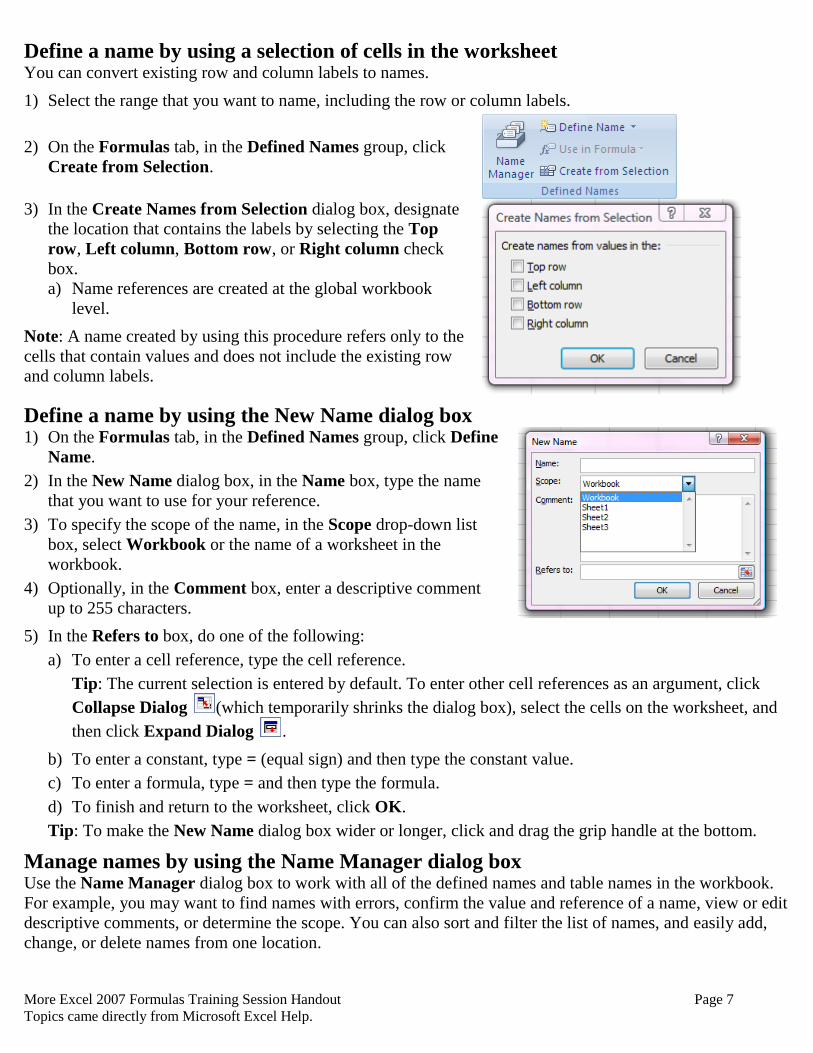
Define a name by using a selection of cells in the worksheet You can convert existing row and column labels to names.

1) Select the range that you want to name, including the row or column labels.

2) On the Formulas tab, in the Defined Names group, click

Create from Selection.

3) In the Create Names from Selection dialog box, designate

the location that contains the labels by selecting the Top

row, Left column, Bottom row, or Right column check

box.

a) Name references are created at the global workbook

level.

Note: A name created by using this procedure refers only to the

cells that contain values and does not include the existing row

and column labels.

Define a name by using the New Name dialog box 1) On the Formulas tab, in the Defined Names group, click Define

Name.

2) In the New Name dialog box, in the Name box, type the name

that you want to use for your reference.

3) To specify the scope of the name, in the Scope drop-down list

box, select Workbook or the name of a worksheet in the

workbook.

4) Optionally, in the Comment box, enter a descriptive comment

up to 255 characters.

5) In the Refers to box, do one of the following:

a) To enter a cell reference, type the cell reference.

Tip: The current selection is entered by default. To enter other cell references as an argument, click

Collapse Dialog (which temporarily shrinks the dialog box), select the cells on the worksheet, and

then click Expand Dialog .

b) To enter a constant, type = (equal sign) and then type the constant value.

c) To enter a formula, type = and then type the formula.

d) To finish and return to the worksheet, click OK.

Tip: To make the New Name dialog box wider or longer, click and drag the grip handle at the bottom.

Manage names by using the Name Manager dialog box Use the Name Manager dialog box to work with all of the defined names and table names in the workbook.

For example, you may want to find names with errors, confirm the value and reference of a name, view or edit

descriptive comments, or determine the scope. You can also sort and filter the list of names, and easily add,

change, or delete names from one location.



To open the Name Manager dialog box, on the Formulas tab, in the Defined Names group, click Name

Manager.

View names The Name Manager dialog box displays the following information about each name in a list box:

This

Column:

Displays:

Icon and

Name

One of the following:

A defined name, which is indicated by a defined name icon.

A table name, which is indicated by a table name icon.

(Tables are not covered in this handout)

Value The current value of the name, such as the results of a formula, a string constant, a cell range,

an error, an array of values, or a placeholder if the formula cannot be evaluated.

Refers To The current reference for the name.

Scope A worksheet name, if the scope is the local worksheet level.

"Workbook", if the scope is the global worksheet level.

Comment Additional information about the name up to 255 characters.



Change a name If you change a defined name or table name, all uses of that name in the workbook are also changed.

1) On the Formulas tab, in the Defined Names group, click Name Manager.

2) In the Name Manager dialog box, click the name that you want to change, and then click Edit.

Tip: You can also double-click the name.

3) In the Edit Name dialog box, in the Name box, type the new name for the reference.

4) In the Refers to box, change the reference , and then click OK.

5) In the Name Manager dialog box, in the Refers to box, change the cell, formula, or constant represented

by the name.

6) To cancel unwanted or accidental changes, click Cancel , or press ESC.

7) To save changes, click Commit , or press ENTER.

Note: The Close button only closes the Name Manager dialog box. It is not required to commit changes

that have already been made.

Delete one or more names 1) On the Formulas tab, in the Defined Names group, click Name Manager.

2) In the Name Manager dialog box, click the name that you want to change.

3) Select one or more names by doing one of the following:

a) To select a name, click it.

b) To select more than one name in a contiguous group, click and drag the names, or press SHIFT and

click the mouse button for each name in the group.

c) To select more than one name in a noncontiguous group, press CTRL and click the mouse button for

each name in the group.

4) Click Delete. (You can also press DELETE on your keyboard.)

5) Click OK to confirm the deletion.

Create Formulas Create a simple formula by using constants and calculation operators 1) Click the cell in which you want to enter the formula.

2) Type = (equal sign).

3) To enter the formula, do one of the following:

a) Type the constants and operators that you want to use in the calculation.

b) Click the cell that contains the value that you want to use in the formula, type the operator that you

want to use, and then click another cell that contains a value.

Tip: You can enter as many constants and operators as you need to achieve the calculation result that

you want.

4) Press ENTER.

Create a formula by using cell references and names The example formulas at the end of this section contain relative references to and names of other cells. The

cell that contains the formula is known as a dependent cell when its value depends on the values in other cells.

For example, cell B2 is a dependent cell if it contains the formula =C2.



1) Click the cell in which you want to enter the formula.

2) In the formula bar , type = (equal sign).

3) Do one of the following:

a) To create a reference: select a cell, a range of cells, a location in another worksheet, or a location in

another workbook.

b) To enter a reference to a named range: press F3, select the name in the Paste name box, and click

OK.

Tip: You can also manually type the defined name.

4) Press ENTER.

Create a formula by using a function 1) Click the cell in which you want to enter the

formula.

2) To start the formula with the function, click Insert

Function button on the formula bar.

a) The Insert Function dialog box opens.

b) You can enter a question that describes what

you want to do in the Search for a function

box (for example, "add numbers" returns the

SUM function), or browse from the categories

in the Or Select a category box.

3) Select the function that you want to use / click

OK.

a) The Function Arguments dialog box opens

4) Enter the arguments.

5) After you complete the formula, press ENTER, or

click OK.

Delete a formula When you delete a formula, the resulting values of the formula is also deleted. However, you can instead

remove the formula only and leave the resulting value of the formula displayed in the cell.

1) To delete formulas along with their resulting values, do the following:

a) Select the cell or range of cells that contains the formula.

b) Press DELETE.

2) To delete formulas without removing their resulting values, do the following:

a) Select the cell or range of cells that contains the formula.

b) On the Home tab, in the Clipboard group, click Copy.

c) On the Home tab, in the Clipboard group, click the arrow below Paste , and then click Paste

Values.



IF function The IF function returns one value if a condition you specify evaluates to TRUE, and another value if that

condition evaluates to FALSE.

For example, the formula =IF(A1>10,"Over 10","10 or less") returns "Over 10" if A1 is greater than 10, and

"10 or less" if A1 is less than or equal to 10.

Syntax

IF(logical_test, value_if_true, [value_if_false])

The IF function syntax has the following arguments:

logical_test: Required. Any value or expression that can be evaluated to TRUE or FALSE.

o For example, A10=100 is a logical expression; if the value in cell A10 is equal to 100, the

expression evaluates to TRUE. Otherwise, the expression evaluates to FALSE.

o This argument can use any comparison calculation operator.

value_if_true: Required. The value that you want to be returned if the logical_test argument evaluates to

TRUE.

o For example, if the value of this argument is the text string "Within budget" and the logical_test

argument evaluates to TRUE, the IF function returns the text "Within budget."

o If logical_test evaluates to TRUE and the value_if_true argument is omitted (that is, there is only a

comma following the logical_test argument), the IF function returns 0 (zero).

o To display the word TRUE, use the logical value TRUE for the value_if_true argument.

value_if_false: Optional. The value that you want to be returned if the logical_test argument evaluates to

FALSE.

o For example, if the value of this argument is the text string "Over budget" and the logical_test

argument evaluates to FALSE, the IF function returns the text "Over budget."

o If logical_test evaluates to FALSE and the value_if_false argument is omitted, (that is, there is no

comma following the value_if_true argument), the IF function returns the logical value FALSE.

o If logical_test evaluates to FALSE and the value of the value_if_false argument is omitted, (that is,

there is a comma following the value_if_true argument, the IF function returns the value 0 (zero).

Up to 64 IF functions can be nested as value_if_true and value_if_false arguments to construct more

elaborate tests.

Example 1

A B

1 Data 2 50 23

Formula Description Result

=IF(A2<=100,"Within budget","Over

budget")

If the number in cell A2 is less than or equal to

100, the formula returns "Within budget."

Otherwise, the function displays "Over budget."

Within

budget

=IF(A2=100,A2+B2,"") If the number in cell A2 is equal to 100, A2 + B2

is calculated and returned. Otherwise, empty text

("") is returned.

Empty

text ("")



Example3

A

1 Score

2 45

3 90

4 78


=IF(A2>89,"A",IF(A2>79,"B",

IF(A2>69,"C",IF(A2>59,"D","F"))))

Assigns a letter grade to the score in cell A2 F

=IF(A3>89,"A",IF(A3>79,"B",

IF(A3>69,"C",IF(A3>59,"D","F"))))

Assigns a letter grade to the score in cell A3 A

=IF(A4>89,"A",IF(A4>79,"B",

IF(A4>69,"C",IF(A4>59,"D","F"))))

Assigns a letter grade to the score in cell A4 C

The preceding example demonstrates how you can nest IF statements. In each formula, the fourth IF

statement is also the value_if_false argument to the third IF statement. Similarly, the third IF statement is the

value_if_false argument to the second IF statement, and the second IF statement is the value_if_false

argument to the first IF statement. For example, if the first logical_test argument (Average>89) evaluates to

TRUE, "A" is returned. If the first logical_test argument evaluates to FALSE, the second IF statement is

evaluated, and so on. You can also use other functions as arguments.

Example 2

A B

1 Actual Expenses Predicted Expenses

2 1500 900

3 500 900

4 500 925


=IF(A2>B2,"Over Budget","OK") Checks whether the expenses in row 2

are over budget

Over Budget

=IF(A3>B3,"Over Budget","OK") Checks whether the expenses in row 3

are over budget

OK



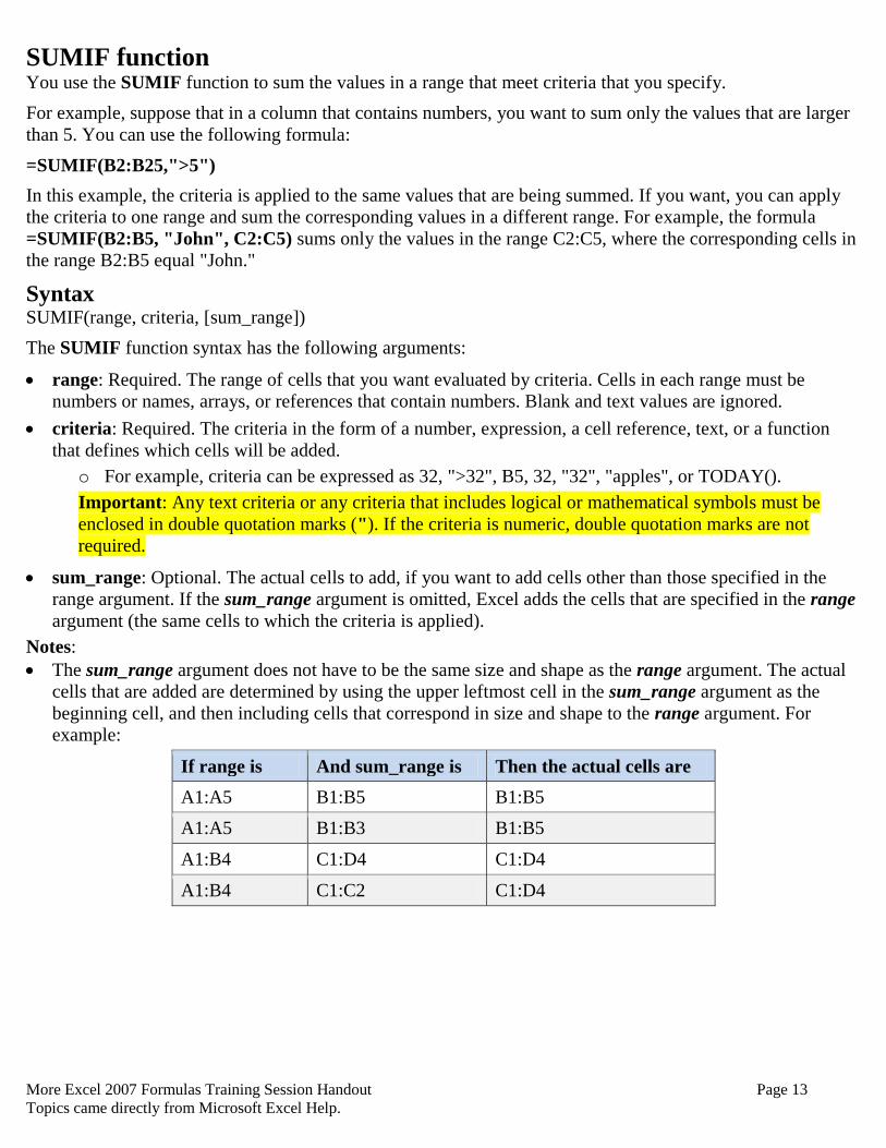
SUMIF function You use the SUMIF function to sum the values in a range that meet criteria that you specify.

For example, suppose that in a column that contains numbers, you want to sum only the values that are larger

than 5. You can use the following formula:

=SUMIF(B2:B25,">5")

In this example, the criteria is applied to the same values that are being summed. If you want, you can apply

the criteria to one range and sum the corresponding values in a different range. For example, the formula

=SUMIF(B2:B5, "John", C2:C5) sums only the values in the range C2:C5, where the corresponding cells in

the range B2:B5 equal "John."

Syntax SUMIF(range, criteria, [sum_range])

The SUMIF function syntax has the following arguments:

range: Required. The range of cells that you want evaluated by criteria. Cells in each range must be

numbers or names, arrays, or references that contain numbers. Blank and text values are ignored.

criteria: Required. The criteria in the form of a number, expression, a cell reference, text, or a function

that defines which cells will be added.

o For example, criteria can be expressed as 32, ">32", B5, 32, "32", "apples", or TODAY().

Important: Any text criteria or any criteria that includes logical or mathematical symbols must be

enclosed in double quotation marks ("). If the criteria is numeric, double quotation marks are not

required.

sum_range: Optional. The actual cells to add, if you want to add cells other than those specified in the

range argument. If the sum_range argument is omitted, Excel adds the cells that are specified in the range

argument (the same cells to which the criteria is applied).

Notes:

The sum_range argument does not have to be the same size and shape as the range argument. The actual

cells that are added are determined by using the upper leftmost cell in the sum_range argument as the

beginning cell, and then including cells that correspond in size and shape to the range argument. For

example:

If range is And sum_range is Then the actual cells are

A1:A5 B1:B5 B1:B5

A1:A5 B1:B3 B1:B5

A1:B4 C1:D4 C1:D4

A1:B4 C1:C2 C1:D4



Example 1

A B C

1 Property Value Commission Data

2 100,000 7,000 250,000

3 200,000 14,000

4 300,000 21,000

5 400,000 28,000


=SUMIF(A2:A5,">160000",B2:B5) Sum of the commissions for

property values over 160,000.

63,000

=SUMIF(A2:A5,">160000") Sum of the property values over

160,000.

900,000

=SUMIF(A2:A5,300000,B2:B5) Sum of the commissions for

property values equal to 300,000.

21,000

=SUMIF(A2:A5,">" & C2,B2:B5) Sum of the commissions for

property values greater than the

value in C2.

49,000

Example 2

A B C

1 Category Food Sales

2 Vegetables Tomatoes 2300

3 Vegetables Celery 5500

4 Fruits Oranges 800

5 Butter 400

6 Vegetables Carrots 4200

7 Fruits Apples 1200


=SUMIF(A2:A7,"Fruits",C2:C7) Sum of the sales of all foods in the "Fruits"

category.

2000

=SUMIF(A2:A7,"Vegetables",C2:C7) Sum of the sales of all foods in the

"Vegetables" category.

12000

=SUMIF(B2:B7,"*es",C2:C7) Sum of the sales of all foods that end in "es"

(Tomatoes, Oranges, and Apples).

4300

=SUMIF(A2:A7,"",C2:C7) Sum of the sales of all foods that do not have a

category specified.

400



SUMIFS function Adds the cells in a range that meet multiple criteria. For example, if you want to sum the numbers in the range

A1:A20 only if the corresponding numbers in B1:B20 are greater than zero (0) and the corresponding

numbers in C1:C20 are less than 10, you can use the following formula:

=SUMIFS(A1:A20, B1:B20, ">0", C1:C20, "<10")

Important: The order of arguments differ between the SUMIFS and SUMIF functions. In particular, the

sum_range argument is the first argument in SUMIFS, but it is the third argument in SUMIF. If you are

copying and editing these similar functions, make sure you put the arguments in the correct order.

Syntax SUMIFS(sum_range, criteria_range1, criteria1, [criteria_range2,criteria2], …)

The SUMIFS function syntax has the following arguments:

sum_range: Required. One or more cells to sum, including numbers or names, ranges, or cell references

that contain numbers. Blank and text values are ignored.

criteria_range1: Required. The first range in which to evaluate the associated criteria.

criteria1: Required. The criteria in the form of a number, expression, cell reference, or text that define

which cells in the criteria_range1 argument will be added.

criteria_range2, criteria2, …:Optional. Additional ranges and their associated criteria. Up to 127

range/criteria pairs are allowed.

Notes:

Each cell in the sum_range argument is summed only if all of the corresponding criteria specified are true

for that cell.

o For example, suppose that a formula contains two criteria_range arguments. If the first cell of

criteria_range1 meets criteria1, and the first cell of criteria_range2 meets critera2, the first cell of

sum_range is added to the sum, and so on, for the remaining cells in the specified ranges.

Cells in the sum_range argument that contain TRUE evaluate to 1; cells in sum_range that contain

FALSE evaluate to 0 (zero).

Unlike the range and criteria arguments in the SUMIF function, in the SUMIFS function, each

criteria_range argument must contain the same number of rows and columns as the sum_range argument.



Example 1

A B C

1 Quantity Sold Product Salesperson

2 5 Apples 1

3 4 Apples 2

4 15 Artichokes 1

5 3 Artichokes 2

6 22 Bananas 1

7 12 Bananas 2

8 10 Carrots 1

9 33 Carrots 2


=SUMIFS(A2:A9, B2:B9, "=A*", C2:C9, 1) Adds the total number of products

sold that begin with "A" and that

were sold by Salesperson 1.

20

=SUMIFS(A2:A9, B2:B9, "<>Bananas", C2:C9, 1) Adds the total number of products

(not including Bananas) sold by

Salesperson 1.

30

Example 2 Adding amounts from bank accounts based on interest paid

A B C D E

1 Totals Account 1 Account 2 Account 3 Account 4

2 Amount in dollars 100 390 8321 500

3 Interest paid (2000) 1% 0.5% 3% 4%

4 Interest paid (2001) 1% 1.3% 2.1% 2%

5 Interest paid (2002) 0.5% 3% 1% 4%


=SUMIFS(B2:E2, B3:E3, ">3%", B4:E4, ">=2%") Total amounts from each bank account

where the interest was greater than 3%

for the year 2000 and greater than or

equal to 2% for the year 2001.

500

=SUMIFS(B2:E2, B5:E5, ">=1%", B5:E5, "<=3%",

B4:E4, ">1%")

Total amounts from each bank account

where the interest was between 1% and

3% for the year 2002 and greater than

1% for the year 2001.

8711



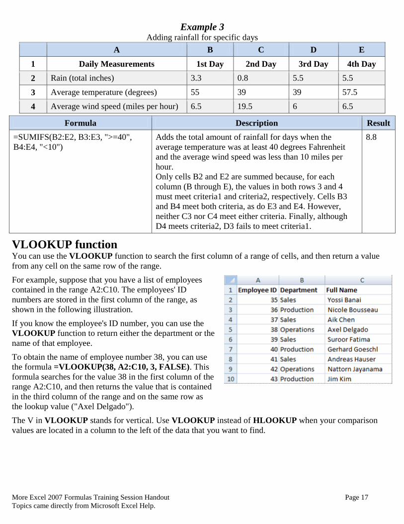
Example 3 Adding rainfall for specific days

A B C D E

1 Daily Measurements 1st Day 2nd Day 3rd Day 4th Day

2 Rain (total inches) 3.3 0.8 5.5 5.5

3 Average temperature (degrees) 55 39 39 57.5

4 Average wind speed (miles per hour) 6.5 19.5 6 6.5


=SUMIFS(B2:E2, B3:E3, ">=40",

B4:E4, "<10")

Adds the total amount of rainfall for days when the

average temperature was at least 40 degrees Fahrenheit

and the average wind speed was less than 10 miles per

hour.

Only cells B2 and E2 are summed because, for each

column (B through E), the values in both rows 3 and 4

must meet criteria1 and criteria2, respectively. Cells B3

and B4 meet both criteria, as do E3 and E4. However,

neither C3 nor C4 meet either criteria. Finally, although

D4 meets criteria2, D3 fails to meet criteria1.

8.8

VLOOKUP function You can use the VLOOKUP function to search the first column of a range of cells, and then return a value

from any cell on the same row of the range.

For example, suppose that you have a list of employees

contained in the range A2:C10. The employees' ID

numbers are stored in the first column of the range, as

shown in the following illustration.

If you know the employee's ID number, you can use the

VLOOKUP function to return either the department or the

name of that employee.

To obtain the name of employee number 38, you can use

the formula =VLOOKUP(38, A2:C10, 3, FALSE). This

formula searches for the value 38 in the first column of the

range A2:C10, and then returns the value that is contained

in the third column of the range and on the same row as

the lookup value ("Axel Delgado").

The V in VLOOKUP stands for vertical. Use VLOOKUP instead of HLOOKUP when your comparison

values are located in a column to the left of the data that you want to find.



Syntax VLOOKUP(lookup_value, table_array, col_index_num, [range_lookup])

The VLOOKUP function syntax has the following arguments:

lookup_value: Required. The value to search in the first column of the table or range.

o The lookup_value argument can be a value or a reference.

o If the value you supply for the lookup_value argument is smaller than the smallest value in the first

column of the table_array argument, VLOOKUP returns the #N/A error value.

table_array: Required. The range of cells that contains the data.

o You can use a reference to a range (for example, A2:D8), or a range name.

o The values in the first column of table_array are the values searched by lookup_value. These

values can be text, numbers, or logical values. Uppercase and lowercase text are equivalent.

col_index_num: Required. The column number in the table_array argument from which the matching

value must be returned.

o A col_index_num argument of 1 returns the value in the first column in table_array; a

col_index_num of 2 returns the value in the second column in table_array, and so on.

o If the col_index_num argument is:

Less than 1, VLOOKUP returns the #VALUE! error value.

Greater than the number of columns in table_array, VLOOKUP returns the #REF! error

value.

range_lookup: Optional. A logical value that specifies whether you want VLOOKUP to find an exact

match or an approximate match:

o If range_lookup is either TRUE or is omitted, an exact or approximate match is returned. If an

exact match is not found, the next largest value that is less than lookup_value is returned.

Important: If range_lookup is either TRUE or is omitted, the values in the first column of

table_array must be placed in ascending sort order; otherwise, VLOOKUP might not return

the correct value.

o If range_lookup is FALSE, the values in the first column of table_array do not need to be sorted.

If the range_lookup argument is FALSE, VLOOKUP will find only an exact match.

If there are two or more values in the first column of table_array that match the

lookup_value, the first value found is used. If an exact match is not found, the error value

#N/A is returned.



Example 1 This example searches the Density column of an atmospheric properties table to

find corresponding values in the Viscosity and Temperature columns.

(The values are for air at 0 degrees Celsius at sea level, or 1 atmosphere.)

A B C

1 Density Viscosity Temperature

2 0.457 3.55 500

3 0.525 3.25 400

4 0.606 2.93 300

5 0.675 2.75 250

6 0.746 2.57 200

7 0.835 2.38 150

8 0.946 2.17 100

9 1.09 1.95 50

10 1.29 1.71 0


=VLOOKUP(1,A2:C10,2) Using an approximate match, searches for the value 1

in column A, finds the largest value less than or equal

to 1 in column A which is 0.946, and then returns the

value from column B in the same row.

2.17

=VLOOKUP(1,A2:C10,3,TRUE) Using an approximate match, searches for the value 1


to 1 in column A, which is 0.946, and then returns the

value from column C in the same row.

100

=VLOOKUP(0.7,A2:C10,3,FALSE) Using an exact match, searches for the value 0.7 in

column A. Because there is no exact match in column

A, an error is returned.

#N/A

=VLOOKUP(0.1,A2:C10,2,TRUE) Using an approximate match, searches for the value 0.1

in column A. Because 0.1 is less than the smallest value

in column A, an error is returned.

#N/A

=VLOOKUP(2,A2:C10,2,TRUE) Using an approximate match, searches for the value 2


to 2 in column A, which is 1.29, and then returns the

value from column B in the same row.

1.71



Example 2 This example searches the Item-ID column of a baby products table and matches values in the Cost and

Markup columns to calculate prices and test conditions.

A B C D

1 Item-ID Item Cost Markup

2 ST-340 Stroller $145.67 30%

3 BI-567 Bib $3.56 40%

4 DI-328 Diapers $21.45 35%

5 WI-989 Wipes $5.12 40%

6 AS-469 Aspirator $2.56 45%


= VLOOKUP("DI-328", A2:D6, 3, FALSE) * (1 +

VLOOKUP("DI-328", A2:D6, 4, FALSE))

Calculates the retail price of diapers

by adding the markup percentage to

the cost.

$28.96

= (VLOOKUP("WI-989", A2:D6, 3, FALSE) * (1 +

VLOOKUP("WI-989", A2:D6, 4, FALSE))) * (1 - 20%)

Calculates the sale price of wipes by

subtracting a specified discount

from the retail price.

$5.73

= IF(VLOOKUP(A2, A2:D6, 3, FALSE) >= 20, "Markup

is " & 100 * VLOOKUP(A2, A2:D6, 4, FALSE) &"%",

"Cost is under $20.00")

If the cost of an item is greater than

or equal to $20.00, displays the

string "Markup is nn%"; otherwise,

displays the string "Cost is under

$20.00".

Markup

is 30%

= IF(VLOOKUP(A3, A2:D6, 3, FALSE) >= 20, "Markup

is: " & 100 * VLOOKUP(A3, A2:D6, 4, FALSE) &"%",

"Cost is $" & VLOOKUP(A3, A2:D6, 3, FALSE))

If the cost of an item is greater than

or equal to $20.00, displays the

string Markup is nn%"; otherwise,

displays the string "Cost is $n.nn".

Cost is

$3.56

Notes:

When searching text values in the first column of table_array, ensure that the data in the first column of

table_array does not contain leading spaces, trailing spaces, inconsistent use of straight ( ' or " ) and curly

( ‗ or ―) quotation marks, or nonprinting characters. In these cases, VLOOKUP might return an incorrect

or unexpected value.

When searching number or date values, ensure that the data in the first column of table_array is not stored

as text values. In this case, VLOOKUP might return an incorrect or unexpected value.

If range_lookup is FALSE and lookup_value is text, you can use the wildcard characters — the question

mark (?) and asterisk (*) — in lookup_value. A question mark matches any single character; an asterisk

matches any sequence of characters. If you want to find an actual question mark or asterisk, type a tilde (~)

preceding the character.



HLOOKUP function Searches for a value in the top row of a table or an array of values, and then returns a value in the same

column from a row you specify in the table or array. Use HLOOKUP when your comparison values are

located in a row across the top of a table of data, and you want to look down a specified number of rows. Use

VLOOKUP when your comparison values are located in a column to the left of the data you want to find.

The H in HLOOKUP stands for "Horizontal."

Syntax HLOOKUP(lookup_value,table_array,row_index_num,range_lookup)

lookup_value is the value to be found in the first row of the table.

o Lookup_value can be a value, a reference, or a text string.

table_array is a table of information in which data is looked up.

o Use a reference to a range or a range name.

o The values in the first row of table_array can be text, numbers, or logical values.

o If range_lookup is TRUE, the values in the first row of table_array must be placed in ascending

order: ...-2, -1, 0, 1, 2,... , A-Z, FALSE, TRUE; otherwise, HLOOKUP may not give the correct

value.

o If range_lookup is FALSE, table_array does not need to be sorted.

o Uppercase and lowercase text are equivalent.

o Sort the values in ascending order, left to right.

row_index_num is the row number in table_array from which the matching value will be returned.

o A row_index_num of 1 returns the first row value in table_array, a row_index_num of 2 returns the

second row value in table_array, and so on.

o If row_index_num is less than 1, HLOOKUP returns the #VALUE! error value; if row_index_num

is greater than the number of rows on table_array, HLOOKUP returns the #REF! error value.

range_lookup is a logical value that specifies whether you want HLOOKUP to find an exact match or an

approximate match.

o If TRUE or omitted, an approximate match is returned. In other words, if an exact match is not

found, the next largest value that is less than lookup_value is returned.

o If FALSE, HLOOKUP will find an exact match. If one is not found, the error value #N/A is

returned.

Notes:

If HLOOKUP can't find lookup_value, and range_lookup is TRUE, it uses the largest value that is less

than lookup_value.

If lookup_value is smaller than the smallest value in the first row of table_array, HLOOKUP returns the

#N/A error value.

If range_lookup is FALSE and lookup_value is text, you can use the wildcard characters, question mark

(?) and asterisk (*), in lookup_value.



Example

A B C

1 Axles Bearings Bolts

2 4 4 9

3 5 7 10

4 6 8 11

Formula Description (Result)

=HLOOKUP("Axles",A1:C4,2,TRUE) Looks up Axles in row 1, and returns the value from

row 2 that's in the same column. (4)

=HLOOKUP("Bearings",A1:C4,3,FALSE) Looks up Bearings in row 1, and returns the value from

row 3 that's in the same column. (7)

=HLOOKUP("B",A1:C4,3,TRUE) Looks up B in row 1, and returns the value from row 3

that's in the same column. Because B is not an exact

match, the next largest value that is less than B is used:

Axles. (5)

=HLOOKUP("Bolts",A1:C4,4) Looks up Bolts in row 1, and returns the value from row

4 that's in the same column. (11)

Avoid common errors when creating formulas The following table summarizes some of the most common errors that you can make when entering a formula

and how to correct those errors:

Make sure that you… More information

Match all open and

close parentheses

Make sure that all parentheses are part of a matching pair. When you create a

formula, Excel displays parentheses in color as they are entered.

Use a colon to indicate a

range

When you refer to a range of cells, use a colon (:) to separate the reference to the

first cell in the range and the reference to the last cell in the range. For example,

A1:A5.

Enter all required

arguments

Some functions have required arguments. Also, make sure that you have not

entered too many arguments.

Nest no more than 64

functions

You can enter, or nest, no more than 64 levels of functions within a function.

Enclose other sheet

names in single

quotation marks

If the formula refers to values or cells on other worksheets or workbooks, and the

name of the other workbook or worksheet contains a nonalphabetical character,

you must enclose its name within single quotation marks ( ' ).

Include the path to

external workbooks

Make sure that each external reference (A reference to a cell or range on a sheet in

another Excel workbook, or a reference to a defined name in another workbook.)

contains a workbook name and the path to the workbook.

Enter numbers without

formatting

Do not format numbers as you enter them in formulas. For example, even if the

value that you want to enter is $1,000, enter 1000 in the formula.

Documents

More Excel 2007 Formulas - Maxwell School of …More Excel 2007 Formulas Training Session Handout Page 2 Topics came directly from Microsoft Excel Help. Overview A formula is a sequence