Embed Size (px)
Citation preview
Exact solutions of semilinear radialSchrodinger equations by group foliation
reduction
Thomas Wolf, Stephen AncoBrock University,
St. Catharines, Ontario, Canada,[email protected], [email protected]
AMMCS 2015, Session SS-RALSMCLWaterloo, 10 June 2015
Outline
Introduction
Group Foliation in 5 Steps
Solving the Group-Resolving System
Solutions for the Nonlinear Heat Equation
The semilinear radial Schrodinger equations
Summary
Interest in Exact Solutions
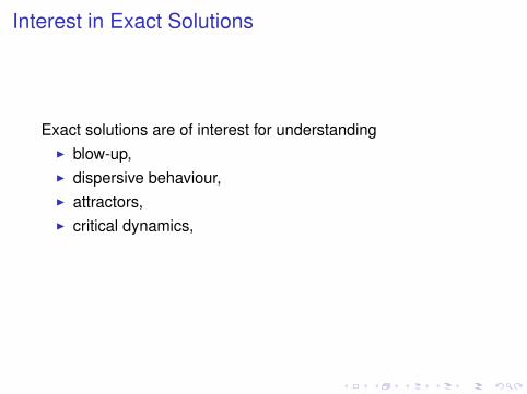
Exact solutions are of interest for understandingI blow-up,
I dispersive behaviour,I attractors,I critical dynamics,
as well as for testing numerical solution methods.

Interest in Exact Solutions
Exact solutions are of interest for understandingI blow-up,I dispersive behaviour,
I attractors,I critical dynamics,
as well as for testing numerical solution methods.

Interest in Exact Solutions
Exact solutions are of interest for understandingI blow-up,I dispersive behaviour,I attractors,
I critical dynamics,as well as for testing numerical solution methods.
Interest in Exact Solutions
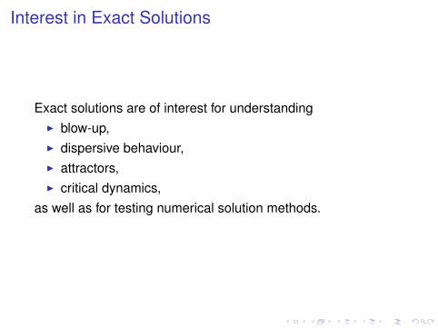
Exact solutions are of interest for understandingI blow-up,I dispersive behaviour,I attractors,I critical dynamics,
as well as for testing numerical solution methods.
Interest in Exact Solutions
Exact solutions are of interest for understandingI blow-up,I dispersive behaviour,I attractors,I critical dynamics,
as well as for testing numerical solution methods.
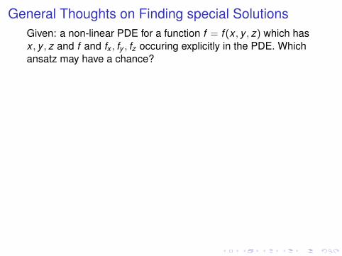
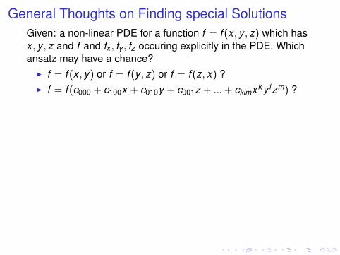
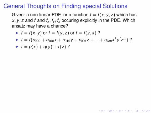
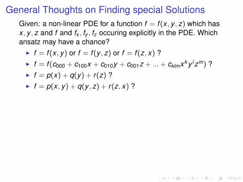
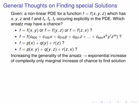
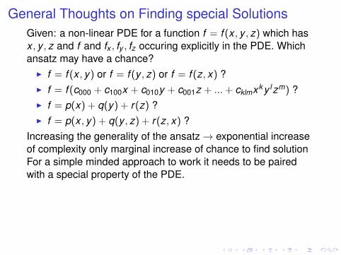
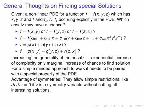
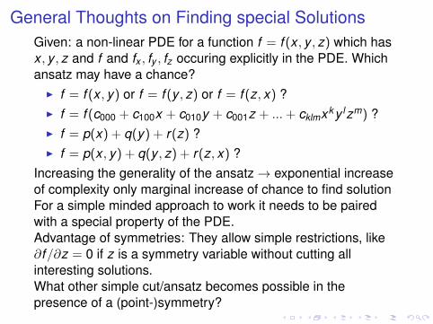
General Thoughts on Finding special SolutionsGiven: a non-linear PDE for a function f = f (x , y , z) which hasx , y , z and f and fx , fy , fz occuring explicitly in the PDE. Whichansatz may have a chance?
I f = f (x , y) or f = f (y , z) or f = f (z, x) ?I f = f (c000 + c100x + c010y + c001z + ...+ cklmxky lzm) ?I f = p(x) + q(y) + r(z) ?I f = p(x , y) + q(y , z) + r(z, x) ?
Increasing the generality of the ansatz→ exponential increaseof complexity only marginal increase of chance to find solutionFor a simple minded approach to work it needs to be pairedwith a special property of the PDE.Advantage of symmetries: They allow simple restrictions, like∂f/∂z = 0 if z is a symmetry variable without cutting allinteresting solutions.What other simple cut/ansatz becomes possible in thepresence of a (point-)symmetry?
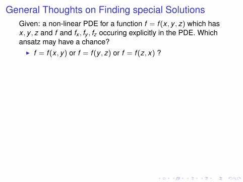
General Thoughts on Finding special SolutionsGiven: a non-linear PDE for a function f = f (x , y , z) which hasx , y , z and f and fx , fy , fz occuring explicitly in the PDE. Whichansatz may have a chance?
I f = f (x , y) or f = f (y , z) or f = f (z, x) ?
I f = f (c000 + c100x + c010y + c001z + ...+ cklmxky lzm) ?I f = p(x) + q(y) + r(z) ?I f = p(x , y) + q(y , z) + r(z, x) ?
Increasing the generality of the ansatz→ exponential increaseof complexity only marginal increase of chance to find solutionFor a simple minded approach to work it needs to be pairedwith a special property of the PDE.Advantage of symmetries: They allow simple restrictions, like∂f/∂z = 0 if z is a symmetry variable without cutting allinteresting solutions.What other simple cut/ansatz becomes possible in thepresence of a (point-)symmetry?
General Thoughts on Finding special SolutionsGiven: a non-linear PDE for a function f = f (x , y , z) which hasx , y , z and f and fx , fy , fz occuring explicitly in the PDE. Whichansatz may have a chance?
I f = f (x , y) or f = f (y , z) or f = f (z, x) ?I f = f (c000 + c100x + c010y + c001z + ...+ cklmxky lzm) ?
I f = p(x) + q(y) + r(z) ?I f = p(x , y) + q(y , z) + r(z, x) ?
Increasing the generality of the ansatz→ exponential increaseof complexity only marginal increase of chance to find solutionFor a simple minded approach to work it needs to be pairedwith a special property of the PDE.Advantage of symmetries: They allow simple restrictions, like∂f/∂z = 0 if z is a symmetry variable without cutting allinteresting solutions.What other simple cut/ansatz becomes possible in thepresence of a (point-)symmetry?
General Thoughts on Finding special SolutionsGiven: a non-linear PDE for a function f = f (x , y , z) which hasx , y , z and f and fx , fy , fz occuring explicitly in the PDE. Whichansatz may have a chance?
I f = f (x , y) or f = f (y , z) or f = f (z, x) ?I f = f (c000 + c100x + c010y + c001z + ...+ cklmxky lzm) ?I f = p(x) + q(y) + r(z) ?
I f = p(x , y) + q(y , z) + r(z, x) ?Increasing the generality of the ansatz→ exponential increaseof complexity only marginal increase of chance to find solutionFor a simple minded approach to work it needs to be pairedwith a special property of the PDE.Advantage of symmetries: They allow simple restrictions, like∂f/∂z = 0 if z is a symmetry variable without cutting allinteresting solutions.What other simple cut/ansatz becomes possible in thepresence of a (point-)symmetry?
General Thoughts on Finding special SolutionsGiven: a non-linear PDE for a function f = f (x , y , z) which hasx , y , z and f and fx , fy , fz occuring explicitly in the PDE. Whichansatz may have a chance?
I f = f (x , y) or f = f (y , z) or f = f (z, x) ?I f = f (c000 + c100x + c010y + c001z + ...+ cklmxky lzm) ?I f = p(x) + q(y) + r(z) ?I f = p(x , y) + q(y , z) + r(z, x) ?
Increasing the generality of the ansatz→ exponential increaseof complexity only marginal increase of chance to find solutionFor a simple minded approach to work it needs to be pairedwith a special property of the PDE.Advantage of symmetries: They allow simple restrictions, like∂f/∂z = 0 if z is a symmetry variable without cutting allinteresting solutions.What other simple cut/ansatz becomes possible in thepresence of a (point-)symmetry?
General Thoughts on Finding special SolutionsGiven: a non-linear PDE for a function f = f (x , y , z) which hasx , y , z and f and fx , fy , fz occuring explicitly in the PDE. Whichansatz may have a chance?
I f = f (x , y) or f = f (y , z) or f = f (z, x) ?I f = f (c000 + c100x + c010y + c001z + ...+ cklmxky lzm) ?I f = p(x) + q(y) + r(z) ?I f = p(x , y) + q(y , z) + r(z, x) ?
Increasing the generality of the ansatz→ exponential increaseof complexity only marginal increase of chance to find solution
For a simple minded approach to work it needs to be pairedwith a special property of the PDE.Advantage of symmetries: They allow simple restrictions, like∂f/∂z = 0 if z is a symmetry variable without cutting allinteresting solutions.What other simple cut/ansatz becomes possible in thepresence of a (point-)symmetry?
General Thoughts on Finding special SolutionsGiven: a non-linear PDE for a function f = f (x , y , z) which hasx , y , z and f and fx , fy , fz occuring explicitly in the PDE. Whichansatz may have a chance?
I f = f (x , y) or f = f (y , z) or f = f (z, x) ?I f = f (c000 + c100x + c010y + c001z + ...+ cklmxky lzm) ?I f = p(x) + q(y) + r(z) ?I f = p(x , y) + q(y , z) + r(z, x) ?
Increasing the generality of the ansatz→ exponential increaseof complexity only marginal increase of chance to find solutionFor a simple minded approach to work it needs to be pairedwith a special property of the PDE.
Advantage of symmetries: They allow simple restrictions, like∂f/∂z = 0 if z is a symmetry variable without cutting allinteresting solutions.What other simple cut/ansatz becomes possible in thepresence of a (point-)symmetry?
General Thoughts on Finding special SolutionsGiven: a non-linear PDE for a function f = f (x , y , z) which hasx , y , z and f and fx , fy , fz occuring explicitly in the PDE. Whichansatz may have a chance?
I f = f (x , y) or f = f (y , z) or f = f (z, x) ?I f = f (c000 + c100x + c010y + c001z + ...+ cklmxky lzm) ?I f = p(x) + q(y) + r(z) ?I f = p(x , y) + q(y , z) + r(z, x) ?
Increasing the generality of the ansatz→ exponential increaseof complexity only marginal increase of chance to find solutionFor a simple minded approach to work it needs to be pairedwith a special property of the PDE.Advantage of symmetries: They allow simple restrictions, like∂f/∂z = 0 if z is a symmetry variable without cutting allinteresting solutions.
What other simple cut/ansatz becomes possible in thepresence of a (point-)symmetry?
General Thoughts on Finding special SolutionsGiven: a non-linear PDE for a function f = f (x , y , z) which hasx , y , z and f and fx , fy , fz occuring explicitly in the PDE. Whichansatz may have a chance?
I f = f (x , y) or f = f (y , z) or f = f (z, x) ?I f = f (c000 + c100x + c010y + c001z + ...+ cklmxky lzm) ?I f = p(x) + q(y) + r(z) ?I f = p(x , y) + q(y , z) + r(z, x) ?
Increasing the generality of the ansatz→ exponential increaseof complexity only marginal increase of chance to find solutionFor a simple minded approach to work it needs to be pairedwith a special property of the PDE.Advantage of symmetries: They allow simple restrictions, like∂f/∂z = 0 if z is a symmetry variable without cutting allinteresting solutions.What other simple cut/ansatz becomes possible in thepresence of a (point-)symmetry?
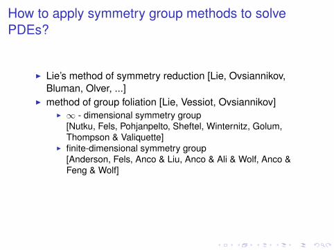
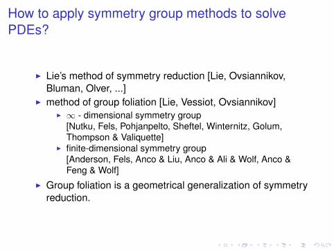
How to apply symmetry group methods to solvePDEs?
I Lie’s method of symmetry reduction [Lie, Ovsiannikov,Bluman, Olver, ...]
I method of group foliation [Lie, Vessiot, Ovsiannikov]I ∞ - dimensional symmetry group
[Nutku, Fels, Pohjanpelto, Sheftel, Winternitz, Golum,Thompson & Valiquette]
I finite-dimensional symmetry group[Anderson, Fels, Anco & Liu, Anco & Ali & Wolf, Anco &Feng & Wolf]
I Group foliation is a geometrical generalization of symmetryreduction.
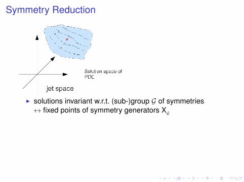
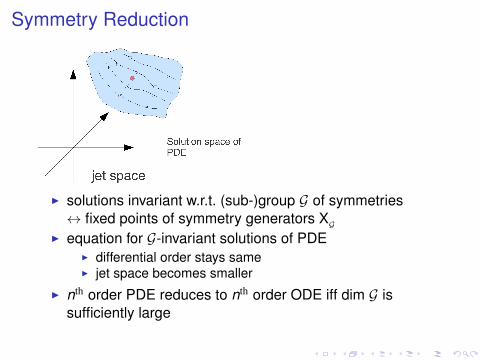
Symmetry Reduction
I solutions invariant w.r.t. (sub-)group G of symmetries↔ fixed points of symmetry generators XG
I equation for G-invariant solutions of PDEI differential order stays sameI jet space becomes smaller
I nth order PDE reduces to nth order ODE iff dim G issufficiently large
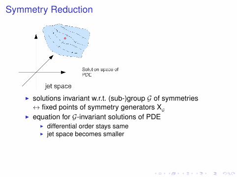
Symmetry Reduction
I solutions invariant w.r.t. (sub-)group G of symmetries↔ fixed points of symmetry generators XG
I equation for G-invariant solutions of PDEI differential order stays sameI jet space becomes smaller
I nth order PDE reduces to nth order ODE iff dim G issufficiently large
Symmetry Reduction
I solutions invariant w.r.t. (sub-)group G of symmetries↔ fixed points of symmetry generators XG
I equation for G-invariant solutions of PDEI differential order stays sameI jet space becomes smaller
I nth order PDE reduces to nth order ODE iff dim G issufficiently large
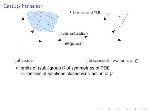
Group Foliation
I orbits of (sub-)group G of symmetries of PDE⇔ families of solutions closed w.r.t. action of G
I equations for G-closed solution familiesI differential order is reducedI size of jet space stays same
I nth order PDE converts into (n− 1)th order system of PDEsI How can one solve the G-invariant system?
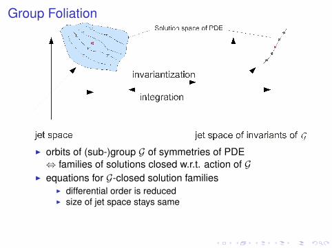
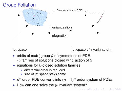
Outline
Introduction
Group Foliation in 5 Steps
Solving the Group-Resolving System
Solutions for the Nonlinear Heat Equation
The semilinear radial Schrodinger equations
Summary
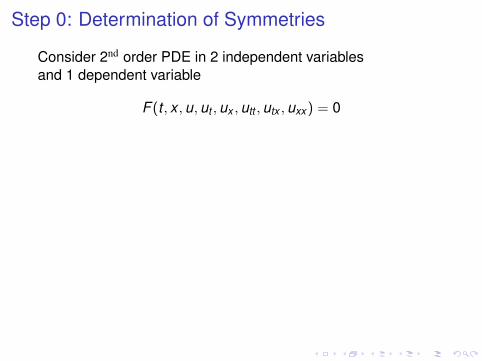
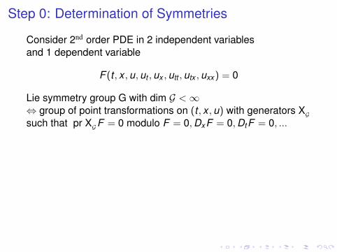
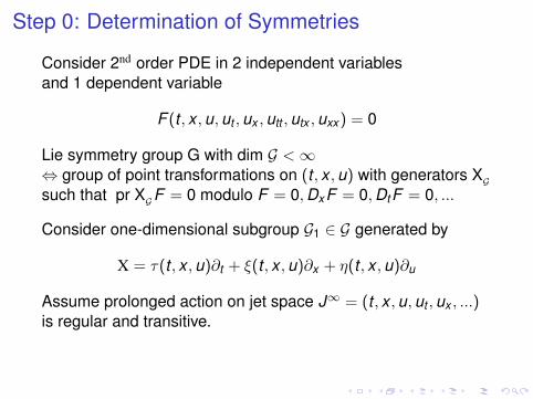
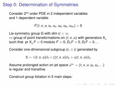
Step 0: Determination of Symmetries
Consider 2nd order PDE in 2 independent variablesand 1 dependent variable
F (t , x ,u,ut ,ux ,utt ,utx ,uxx ) = 0
Lie symmetry group G with dim G <∞⇔ group of point transformations on (t , x ,u) with generators XGsuch that pr XGF = 0 modulo F = 0,DxF = 0,DtF = 0, ...
Consider one-dimensional subgroup G1 ∈ G generated by
X = τ(t , x ,u)∂t + ξ(t , x ,u)∂x + η(t , x ,u)∂u
Assume prolonged action on jet space J∞ = (t , x ,u,ut ,ux , ...)is regular and transitive.
Construct group foliation in 5 main steps:
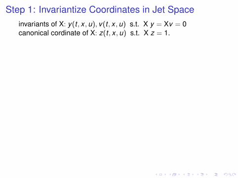
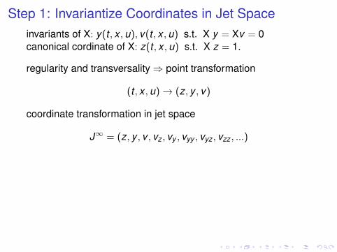
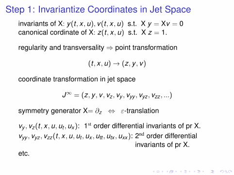
Step 1: Invariantize Coordinates in Jet Spaceinvariants of X: y(t , x ,u), v(t , x ,u) s.t. X y = Xv = 0canonical cordinate of X: z(t , x ,u) s.t. X z = 1.
regularity and transversality⇒ point transformation
(t , x ,u)→ (z, y , v)
coordinate transformation in jet space
J∞ = (z, y , v , vz , vy , vyy , vyz , vzz , ...)
symmetry generator X= ∂z ⇔ ε-translation
vy , vz(t , x ,u,ut ,ux ): 1st order differential invariants of pr X.vyy , vyz , vzz(t , x ,u,ut ,ux ,utt ,utx ,uxx ): 2nd order differential
invariants of pr X.etc.
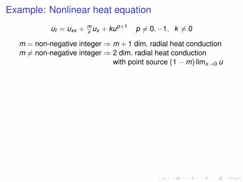
Example: Nonlinear heat equation
ut = uxx + mx ux + kup+1 p 6= 0,−1, k 6= 0
m = non-negative integer⇒ m + 1 dim. radial heat conductionm 6= non-negative integer⇒ 2 dim. radial heat conduction
with point source (1−m) limx→0 u
symmetry group generated byX = ∂t time translationX = ∂x (if m = 0) space translationX = 2t∂t + x∂x − 2
p u∂u scaling
consider scaling symmetry X= 2t∂t + x∂x − 2p u∂u
invariants ζ(t , x ,u) s.t. Xζ = 0 = 2tζt + xζx − 2p uζu
⇒ ζ is function of y = x2
t , v = x2/pu
canonical coordinate z(t , x ,u) s.t. Xz = 1⇒ z = ln x + (function of y , v) = ln x (for simplicity)

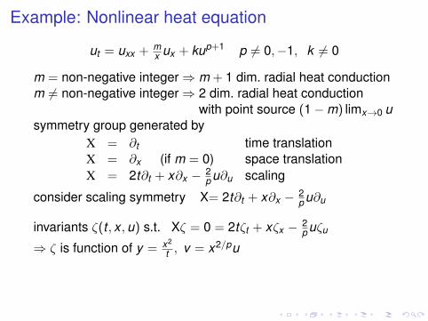
Example: Nonlinear heat equation
ut = uxx + mx ux + kup+1 p 6= 0,−1, k 6= 0
m = non-negative integer⇒ m + 1 dim. radial heat conductionm 6= non-negative integer⇒ 2 dim. radial heat conduction
with point source (1−m) limx→0 usymmetry group generated by
X = ∂t time translationX = ∂x (if m = 0) space translationX = 2t∂t + x∂x − 2
p u∂u scaling
consider scaling symmetry X= 2t∂t + x∂x − 2p u∂u
invariants ζ(t , x ,u) s.t. Xζ = 0 = 2tζt + xζx − 2p uζu
⇒ ζ is function of y = x2
t , v = x2/pu
canonical coordinate z(t , x ,u) s.t. Xz = 1⇒ z = ln x + (function of y , v) = ln x (for simplicity)
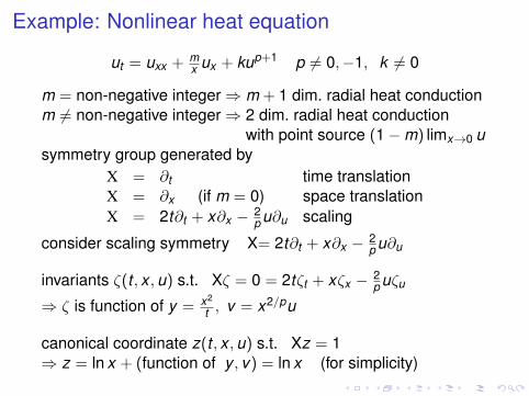
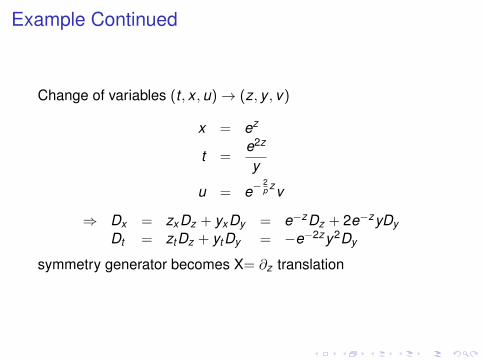
Example Continued
Change of variables (t , x ,u)→ (z, y , v)
x = ez
t =e2z
y
u = e−2p zv
⇒ Dx = zxDz + yxDy = e−zDz + 2e−zyDyDt = ztDz + ytDy = −e−2zy2Dy
symmetry generator becomes X= ∂z translation
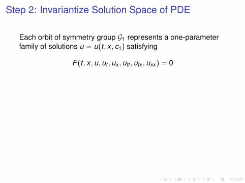
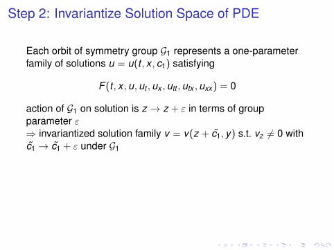
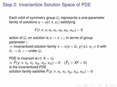
Step 2: Invariantize Solution Space of PDE
Each orbit of symmetry group G1 represents a one-parameterfamily of solutions u = u(t , x , c1) satisfying
F (t , x ,u,ut ,ux ,utt ,utx ,uxx ) = 0
action of G1 on solution is z → z + ε in terms of groupparameter ε⇒ invariantized solution family v = v(z + c1, y) s.t. vz 6= 0 withc1 → c1 + ε under G1
PDE is invariant w.r.t. X = ∂z⇔ F (y , v , vy , vz , vyy , vyz , vzz) = 0 (Fz = XF = 0)is the invariantized PDEsolution family satisfies F (y , v , vy , vz , vyy , vyz , vzz) = 0
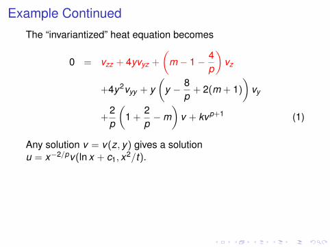
Example Continued
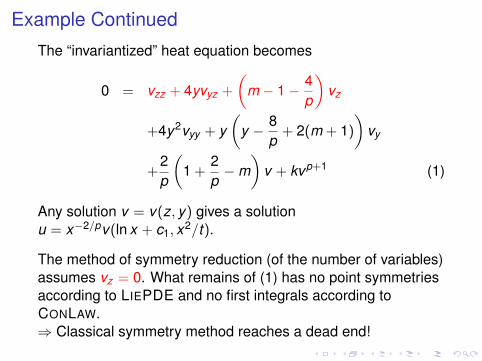
The “invariantized” heat equation becomes
0 = vzz + 4yvyz +
(m − 1− 4
p
)vz
+4y2vyy + y(
y − 8p
+ 2(m + 1)
)vy
+2p
(1 +
2p−m
)v + kvp+1 (1)
Any solution v = v(z, y) gives a solutionu = x−2/pv(ln x + c1, x2/t).
The method of symmetry reduction (of the number of variables)assumes vz = 0. What remains of (1) has no point symmetriesaccording to LIEPDE and no first integrals according toCONLAW.⇒ Classical symmetry method reaches a dead end!
Example Continued
The “invariantized” heat equation becomes
0 = vzz + 4yvyz +
(m − 1− 4
p
)vz
+4y2vyy + y(
y − 8p
+ 2(m + 1)
)vy
+2p
(1 +
2p−m
)v + kvp+1 (1)
Any solution v = v(z, y) gives a solutionu = x−2/pv(ln x + c1, x2/t).
The method of symmetry reduction (of the number of variables)assumes vz = 0. What remains of (1) has no point symmetriesaccording to LIEPDE and no first integrals according toCONLAW.⇒ Classical symmetry method reaches a dead end!
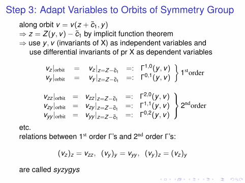
Step 3: Adapt Variables to Orbits of Symmetry Groupalong orbit v = v(z + c1, y)⇒ z = Z (y , v)− c1 by implicit function theorem⇒ use y , v (invariants of X) as independent variables and
use differential invariants of pr X as dependent variables
vz |orbit = vz |z=Z−c1=: Γ1,0(y , v)
vy |orbit = vy |z=Z−c1=: Γ0,1(y , v)
}1storder
vzz |orbit = vzz |z=Z−c1=: Γ2,0(y , v)
vzy |orbit = vzy |z=Z−c1=: Γ1,1(y , v)
vyy |orbit = vyy |z=Z−c1=: Γ0,2(y , v)
2ndorder
etc.relations between 1st order Γ’s and 2nd order Γ’s:
(vz)z = vzz , (vy )y = vyy , (vy )z = (vz)y
are called syzygys
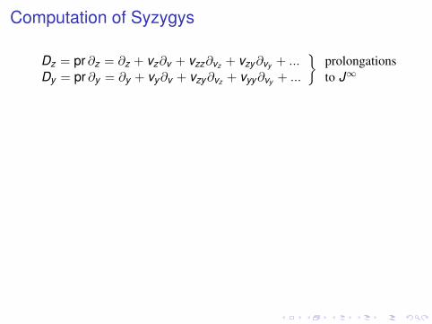
Computation of Syzygys
Dz = pr ∂z = ∂z + vz∂v + vzz∂vz + vzy∂vy + ...Dy = pr ∂y = ∂y + vy∂v + vzy∂vz + vyy∂vy + ...
}prolongationsto J∞
evaluate along orbits of G1
Dz |orbit = 0 + Γ1,0∂v + Γ2,0∂Γ1,0 + Γ1,1∂Γ0,1 + ... ≡ Dz
Dy |orbit = ∂y + Γ0,1∂v + Γ1,1∂Γ1,0 + Γ0,2∂Γ0,1 + ... ≡ Dy
⇒ Γ2,0 = DzΓ1,0 = Γ1,0Γ1,0v
Γ0,2 = Dy Γ0,1 = Γ0,1y + Γ0,1Γ1,0
v
Γ1,1 = DzΓ0,1 = Γ1,0Γ0,1v
= Dy Γ1,0 = Γ1,0y + Γ0,1Γ1,0
v
syzygys
etc.
J∞|orbit = (y , v , Γ1,0, Γ0,1, Γ2,0, Γ1,1, Γ0,2, ...) modulo syzygys
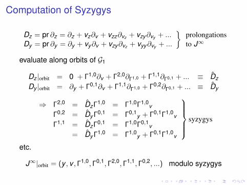
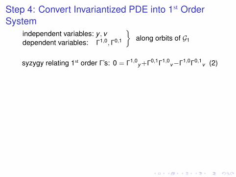
Step 4: Convert Invariantized PDE into 1st OrderSystem
independent variables: y , vdependent variables: Γ1,0, Γ0,1
}along orbits of G1
syzygy relating 1st order Γ’s: 0 = Γ1,0y +Γ0,1Γ1,0
v−Γ1,0Γ0,1v (2)
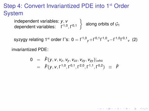
invariantized PDE:
0 = F (y , v , vz , vy , vzz , vzy , vyy )|orbit
= F (y , v , Γ1,0, Γ0,1, Γ2,0, Γ1,1, Γ0,2) ≡ F
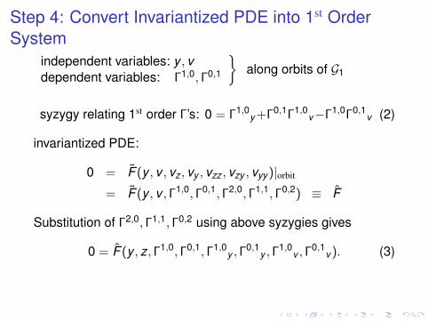
Substitution of Γ2,0, Γ1,1, Γ0,2 using above syzygies gives
0 = F (y , z, Γ1,0, Γ0,1, Γ1,0y , Γ
0,1y , Γ
1,0v , Γ
0,1v ). (3)
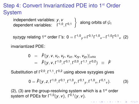
(2), (3) are the group-resolving system which is a 1st ordersystem of PDEs for Γ1,0(y , v), Γ0,1(y , v).
Step 4: Convert Invariantized PDE into 1st OrderSystem
independent variables: y , vdependent variables: Γ1,0, Γ0,1
}along orbits of G1
syzygy relating 1st order Γ’s: 0 = Γ1,0y +Γ0,1Γ1,0
v−Γ1,0Γ0,1v (2)
invariantized PDE:
0 = F (y , v , vz , vy , vzz , vzy , vyy )|orbit
= F (y , v , Γ1,0, Γ0,1, Γ2,0, Γ1,1, Γ0,2) ≡ F
Substitution of Γ2,0, Γ1,1, Γ0,2 using above syzygies gives
0 = F (y , z, Γ1,0, Γ0,1, Γ1,0y , Γ
0,1y , Γ
1,0v , Γ
0,1v ). (3)
(2), (3) are the group-resolving system which is a 1st ordersystem of PDEs for Γ1,0(y , v), Γ0,1(y , v).
Example Continued
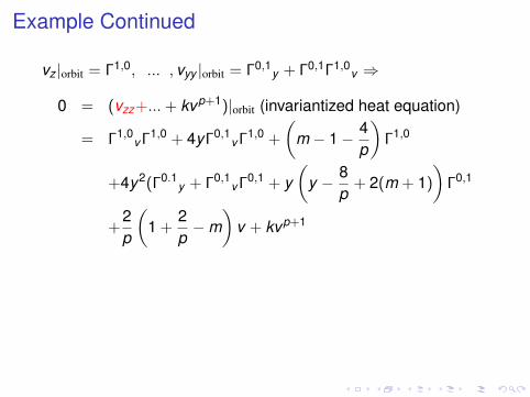
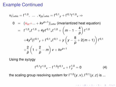
vz |orbit = Γ1,0, ... , vyy |orbit = Γ0,1y + Γ0,1Γ1,0
v ⇒
0 = (vzz+...+ kvp+1)|orbit (invariantized heat equation)
= Γ1,0v Γ1,0 + 4yΓ0,1
v Γ1,0 +
(m − 1− 4
p
)Γ1,0
+4y2(Γ0.1y + Γ0,1
v Γ0,1 + y(
y − 8p
+ 2(m + 1)
)Γ0,1
+2p
(1 +
2p−m
)v + kvp+1
Using the syzygy
Γ0,1Γ1,0v − Γ1,0Γ0,1
v + Γ1,0y = 0 (4)
the scaling group resolving system for Γ1,0(y , v), Γ0,1(y , z) is ...
Example Continued
vz |orbit = Γ1,0, ... , vyy |orbit = Γ0,1y + Γ0,1Γ1,0
v ⇒
0 = (vzz+...+ kvp+1)|orbit (invariantized heat equation)
= Γ1,0v Γ1,0 + 4yΓ0,1
v Γ1,0 +
(m − 1− 4
p
)Γ1,0
+4y2(Γ0.1y + Γ0,1
v Γ0,1 + y(
y − 8p
+ 2(m + 1)
)Γ0,1
+2p
(1 +
2p−m
)v + kvp+1
Using the syzygy
Γ0,1Γ1,0v − Γ1,0Γ0,1
v + Γ1,0y = 0 (4)
the scaling group resolving system for Γ1,0(y , v), Γ0,1(y , z) is ...
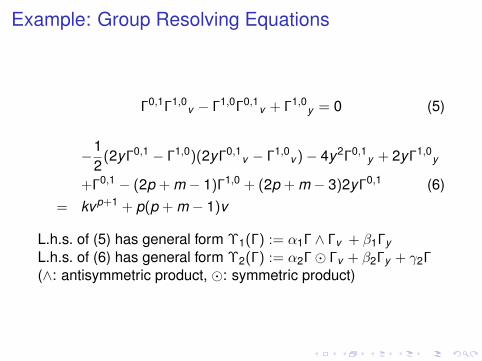
Example: Group Resolving Equations
Γ0,1Γ1,0v − Γ1,0Γ0,1
v + Γ1,0y = 0 (5)
−12
(2yΓ0,1 − Γ1,0)(2yΓ0,1v − Γ1,0
v )− 4y2Γ0,1y + 2yΓ1,0
y
+Γ0,1 − (2p + m − 1)Γ1,0 + (2p + m − 3)2yΓ0,1 (6)= kvp+1 + p(p + m − 1)v
L.h.s. of (5) has general form Υ1(Γ) := α1Γ ∧ Γv + β1ΓyL.h.s. of (6) has general form Υ2(Γ) := α2Γ� Γv + β2Γy + γ2Γ(∧: antisymmetric product, �: symmetric product)
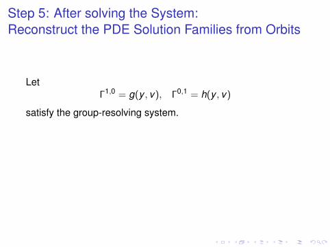
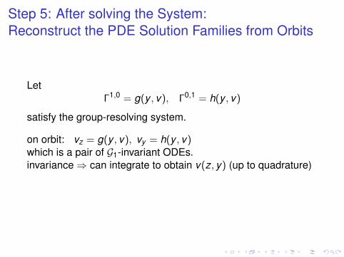
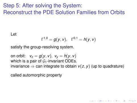
Step 5: After solving the System:Reconstruct the PDE Solution Families from Orbits
LetΓ1,0 = g(y , v), Γ0,1 = h(y , v)
satisfy the group-resolving system.
on orbit: vz = g(y , v), vy = h(y , v)which is a pair of G1-invariant ODEs.invariance⇒ can integrate to obtain v(z, y) (up to quadrature)
called automorphic property
Outline
Introduction
Group Foliation in 5 Steps
Solving the Group-Resolving System
Solutions for the Nonlinear Heat Equation
The semilinear radial Schrodinger equations
Summary
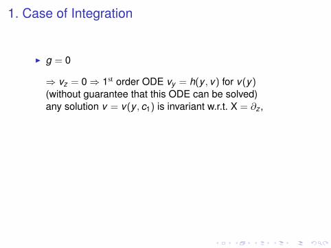
1. Case of Integration
I g = 0
⇒ vz = 0⇒ 1st order ODE vy = h(y , v) for v(y)(without guarantee that this ODE can be solved)any solution v = v(y , c1) is invariant w.r.t. X = ∂z ,
change variables (z, y , v)→ (t , x ,u)
⇒ solution u = u(t , x , c1) invariant w.r.t. G1,
⇒ one-parameter family of fixed points of G1
⇒ this case is equivalent to the symmetry method
2. Case of Integration
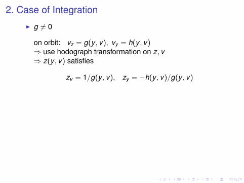
I g 6= 0
on orbit: vz = g(y , v), vy = h(y , v)⇒ use hodograph transformation on z, v⇒ z(y , v) satisfies
zv = 1/g(y , v), zy = −h(y , v)/g(y , v)
solve by line integral formula
z + c1 =
∫1
g(y , v)dv − h(y , v)
g(y , v)dy (path− independent)
⇒ implicit solution v = v(z + c1, y)
change of variables (z, y , v)→ (t , x ,u)⇒ solution u = u(t , x , c1) closed family w.r.t. G1, i.e.one-dimensional orbit of G1
2. Case of Integration
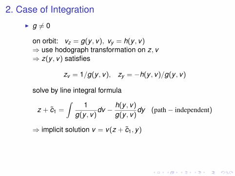
I g 6= 0
on orbit: vz = g(y , v), vy = h(y , v)⇒ use hodograph transformation on z, v⇒ z(y , v) satisfies
zv = 1/g(y , v), zy = −h(y , v)/g(y , v)
solve by line integral formula
z + c1 =
∫1
g(y , v)dv − h(y , v)
g(y , v)dy (path− independent)
⇒ implicit solution v = v(z + c1, y)
change of variables (z, y , v)→ (t , x ,u)⇒ solution u = u(t , x , c1) closed family w.r.t. G1, i.e.one-dimensional orbit of G1
2. Case of Integration
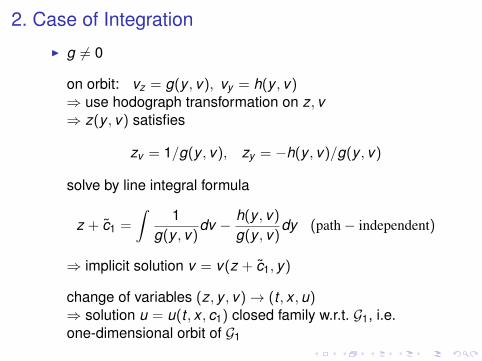
I g 6= 0
on orbit: vz = g(y , v), vy = h(y , v)⇒ use hodograph transformation on z, v⇒ z(y , v) satisfies
zv = 1/g(y , v), zy = −h(y , v)/g(y , v)
solve by line integral formula
z + c1 =
∫1
g(y , v)dv − h(y , v)
g(y , v)dy (path− independent)
⇒ implicit solution v = v(z + c1, y)
change of variables (z, y , v)→ (t , x ,u)⇒ solution u = u(t , x , c1) closed family w.r.t. G1, i.e.one-dimensional orbit of G1
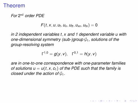
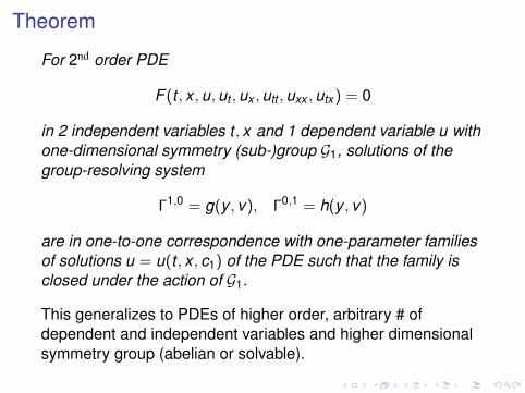
Theorem
For 2nd order PDE
F (t , x ,u,ut ,ux ,utt ,uxx ,utx ) = 0
in 2 independent variables t , x and 1 dependent variable u withone-dimensional symmetry (sub-)group G1, solutions of thegroup-resolving system
Γ1,0 = g(y , v), Γ0,1 = h(y , v)
are in one-to-one correspondence with one-parameter familiesof solutions u = u(t , x , c1) of the PDE such that the family isclosed under the action of G1.
This generalizes to PDEs of higher order, arbitrary # ofdependent and independent variables and higher dimensionalsymmetry group (abelian or solvable).
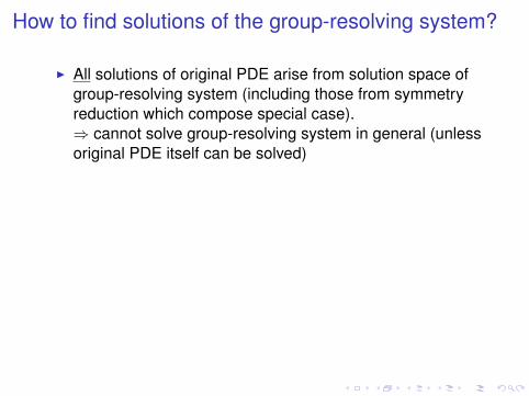
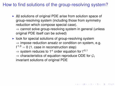
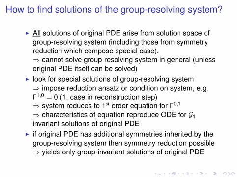
How to find solutions of the group-resolving system?
I All solutions of original PDE arise from solution space ofgroup-resolving system (including those from symmetryreduction which compose special case).⇒ cannot solve group-resolving system in general (unlessoriginal PDE itself can be solved)
I look for special solutions of group-resolving system⇒ impose reduction ansatz or condition on system, e.g.Γ1,0 = 0 (1. case in reconstruction step)⇒ system reduces to 1st order equation for Γ0,1
⇒ characteristics of equation reproduce ODE for G1invariant solutions of original PDE
I if original PDE has additional symmetries inherited by thegroup-resolving system then symmetry reduction possible⇒ yields only group-invariant solutions of original PDE
Reduction Methods for Group-Resolving Systems
I reduction under hidden symmetries
I Bluman’s nonclassical method (invariant surface condition)Clarkson’s direct method and more general functionalseparation methods
I (successfully used by us:)separation ansatz tailored to certain homogeneity featuresof group-resolving system
I yields explicit solutionsI semi-algorithmic⇒ suited to computer algebra (e.g.
Crack/Reduce)I used for group-resolving systems coming from semilinear
PDEs with power nonlinearities
Reduction Methods for Group-Resolving Systems
I reduction under hidden symmetriesI Bluman’s nonclassical method (invariant surface condition)
Clarkson’s direct method and more general functionalseparation methods
I (successfully used by us:)separation ansatz tailored to certain homogeneity featuresof group-resolving system
I yields explicit solutionsI semi-algorithmic⇒ suited to computer algebra (e.g.
Crack/Reduce)I used for group-resolving systems coming from semilinear
PDEs with power nonlinearities
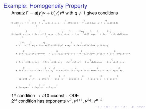
Example: Homogeneity PropertyAnsatz Γ = a(y)v + b(y)vq with q 6= 1 gives conditions
q q q q q0=a10 *v + v *b10 + v *a01*b10*q - v *a01*b10 - v *a10*b01*q + v *a10*b01
y y
2 q p 2 2*q 2 2 2*q0=4*a10 *v *y + 4*v *b10 *v*y - 2*v *k*v - 4*v *b01 *q*y + 4*v *b01*b10*q*y
y y
2*q 2 q 2 q- v *b10 *q - 4*v *a01*b01*(q+1)*v*y + 2*v *a01*b10*(q+1)*v*y
q q q q+ 2*v *a10*b01*q*v*y + 2*v *a10*b01*v*y - v *a10*b10*(q+1)*v + 4*v *b01*m*v*y
q q q q q+ 8*v *b01*p*v*y - 12*v *b01*v*y + 2*v *b01*v - 2*v *b10*m*v - 4*v *b10*p*v
q 2 2 2 2 2 2+ 2*v *b10*v - 4*a01 *v *y + 4*a01*a10*v *y + 4*a01*m*v *y + 8*a01*p*v *y
2 2 2 2 2 2 2- 12*a01*v *y + 2*a01*v - a10 *v - 2*a10*m*v - 4*a10*p*v + 2*a10*v
2 2 2 2+ 2*m*p*v + 2*p *v - 2*p*v
1st condition→ a10 =const + ODE2nd condition has exponents v2, vq+1, v2q, vp+2
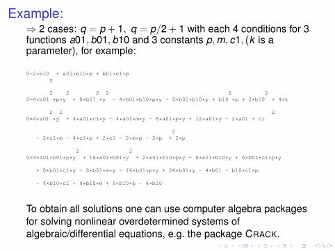
Example:⇒ 2 cases: q = p + 1, q = p/2 + 1 with each 4 conditions for 3functions a01,b01,b10 and 3 constants p,m, c1, (k is aparameter), for example:
0=2*b10 + a01*b10*p + b01*c1*py
2 2 2 2 2 20=4*b01 *p*y + 8*b01 *y - 4*b01*b10*p*y - 8*b01*b10*y + b10 *p + 2*b10 + 4*k
2 2 20=4*a01 *y + 4*a01*c1*y - 4*a01*m*y - 8*a01*p*y + 12*a01*y - 2*a01 + c1
2- 2*c1*m - 4*c1*p + 2*c1 - 2*m*p - 2*p + 2*p
2 20=4*a01*b01*p*y + 16*a01*b01*y + 2*a01*b10*p*y - 8*a01*b10*y + 6*b01*c1*p*y
+ 8*b01*c1*y - 8*b01*m*y - 16*b01*p*y + 24*b01*y - 4*b01 - b10*c1*p
- 4*b10*c1 + 4*b10*m + 8*b10*p - 4*b10
To obtain all solutions one can use computer algebra packagesfor solving nonlinear overdetermined systems ofalgebraic/differential equations, e.g. the package CRACK.
Outline
Introduction
Group Foliation in 5 Steps
Solving the Group-Resolving System
Solutions for the Nonlinear Heat Equation
The semilinear radial Schrodinger equations
Summary
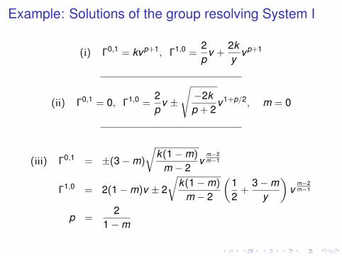
Example: Solutions of the group resolving System I
(i) Γ0,1 = kvp+1, Γ1,0 =2p
v +2ky
vp+1
(ii) Γ0,1 = 0, Γ1,0 =2p
v ±
√−2kp + 2
v1+p/2, m = 0
(iii) Γ0,1 = ±(3−m)
√k(1−m)
m − 2v
m−2m−1
Γ1,0 = 2(1−m)v ± 2
√k(1−m)
m − 2
(12
+3−m
y
)v
m−2m−1
p =2
1−m
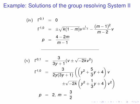
Example: Solutions of the group resolving System II
(iv) Γ0,1 = 0
Γ1,0 = ±√
k(1−m)v1
m−1 − (m − 1)2
m − 2v
p =4− 2mm − 1
(v) Γ0,1 =3
3y + 1(v ±
√−2kv2)
Γ1,0 =3
2y(3y + 1)
((y2 +
53
y + 4)
v
±√−2k
(y2 +
13
y + 4)
v2)
p = 2, m =32
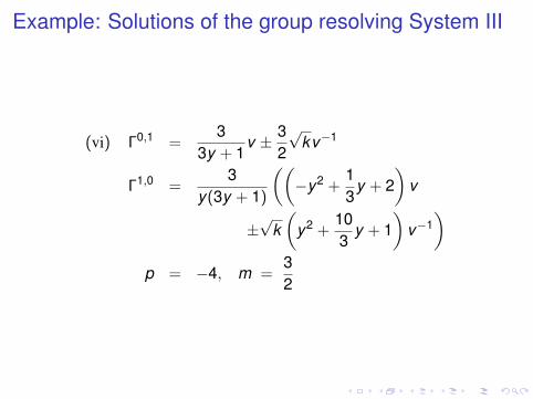
Example: Solutions of the group resolving System III
(vi) Γ0,1 =3
3y + 1v ± 3
2
√kv−1
Γ1,0 =3
y(3y + 1)
((−y2 +
13
y + 2)
v
±√
k(
y2 +103
y + 1)
v−1)
p = −4, m =32
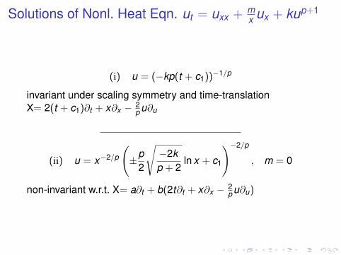
Solutions of Nonl. Heat Eqn. ut = uxx +mx ux + kup+1
(i) u = (−kp(t + c1))−1/p
invariant under scaling symmetry and time-translationX= 2(t + c1)∂t + x∂x − 2
p u∂u
(ii) u = x−2/p
(±p
2
√−2kp + 2
ln x + c1
)−2/p
, m = 0
non-invariant w.r.t. X= a∂t + b(2t∂t + x∂x − 2p u∂u)
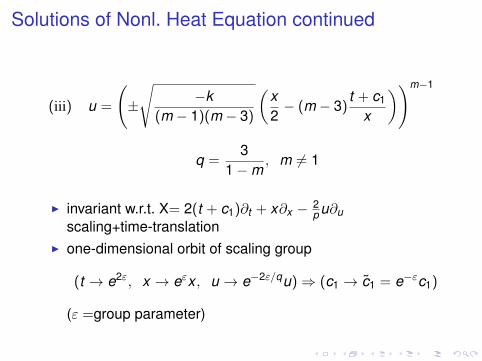
Solutions of Nonl. Heat Equation continued
(iii) u =
(±
√−k
(m − 1)(m − 3)
(x2− (m − 3)
t + c1
x
))m−1
q =3
1−m, m 6= 1
I invariant w.r.t. X= 2(t + c1)∂t + x∂x − 2p u∂u
scaling+time-translationI one-dimensional orbit of scaling group
(t → e2ε, x → eεx , u → e−2ε/qu)⇒ (c1 → c1 = e−εc1)
(ε =group parameter)
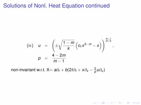
Solutions of Nonl. Heat Equation continued
(iv) u =
(±√
1−mk
(c1x3−m − x
))m−1m−2
,
p =4− 2mm − 1
non-invariant w.r.t. X= a∂t + b(2t∂t + x∂x − 2p u∂u)
Solutions of Nonl. Heat Equation continued
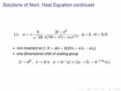
(v) u = ± 5√−2k
3t + x2
x(15t + x2) + c1x1/2 , q = 2, m = 3/2
I non-invariant w.r.t. X = a∂t + b(2t∂t + x∂x − u∂u)
I one-dimensional orbit of scaling group
(t → e2ε, x → eεx , u → e−εu)⇒ (c1 → c1 = e−1/2εc1)
Solutions of Nonl. Heat Equation continued
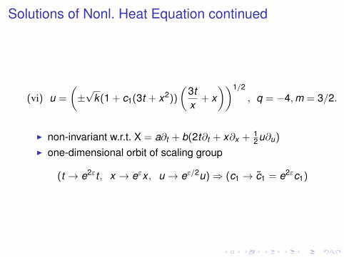
(vi) u =
(±√
k(1 + c1(3t + x2))
(3tx
+ x))1/2
, q = −4,m = 3/2.
I non-invariant w.r.t. X = a∂t + b(2t∂t + x∂x + 12u∂u)
I one-dimensional orbit of scaling group
(t → e2εt , x → eεx , u → eε/2u)⇒ (c1 → c1 = e2εc1)

Outline
Introduction
Group Foliation in 5 Steps
Solving the Group-Resolving System
Solutions for the Nonlinear Heat Equation
The semilinear radial Schrodinger equations
Summary
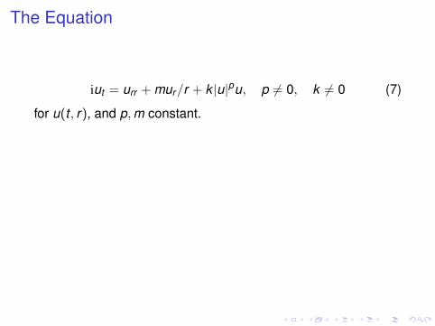
The Equation
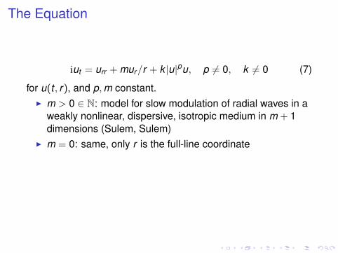
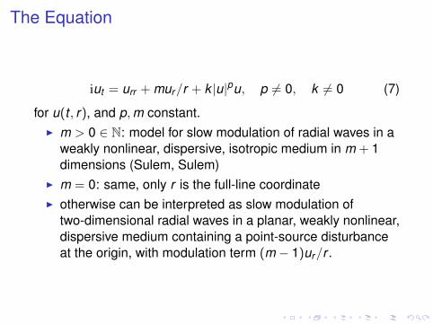
iut = urr + mur/r + k |u|pu, p 6= 0, k 6= 0 (7)
for u(t , r), and p,m constant.
I m > 0 ∈ N: model for slow modulation of radial waves in aweakly nonlinear, dispersive, isotropic medium in m + 1dimensions (Sulem, Sulem)
I m = 0: same, only r is the full-line coordinateI otherwise can be interpreted as slow modulation of
two-dimensional radial waves in a planar, weakly nonlinear,dispersive medium containing a point-source disturbanceat the origin, with modulation term (m − 1)ur/r .
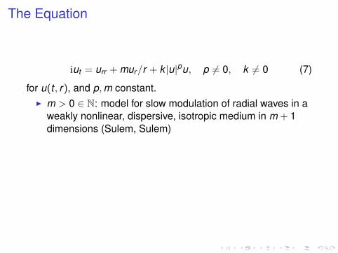
The Equation
iut = urr + mur/r + k |u|pu, p 6= 0, k 6= 0 (7)
for u(t , r), and p,m constant.I m > 0 ∈ N: model for slow modulation of radial waves in a
weakly nonlinear, dispersive, isotropic medium in m + 1dimensions (Sulem, Sulem)
I m = 0: same, only r is the full-line coordinateI otherwise can be interpreted as slow modulation of
two-dimensional radial waves in a planar, weakly nonlinear,dispersive medium containing a point-source disturbanceat the origin, with modulation term (m − 1)ur/r .
The Equation
iut = urr + mur/r + k |u|pu, p 6= 0, k 6= 0 (7)
for u(t , r), and p,m constant.I m > 0 ∈ N: model for slow modulation of radial waves in a
weakly nonlinear, dispersive, isotropic medium in m + 1dimensions (Sulem, Sulem)
I m = 0: same, only r is the full-line coordinate
I otherwise can be interpreted as slow modulation oftwo-dimensional radial waves in a planar, weakly nonlinear,dispersive medium containing a point-source disturbanceat the origin, with modulation term (m − 1)ur/r .
The Equation
iut = urr + mur/r + k |u|pu, p 6= 0, k 6= 0 (7)
for u(t , r), and p,m constant.I m > 0 ∈ N: model for slow modulation of radial waves in a
weakly nonlinear, dispersive, isotropic medium in m + 1dimensions (Sulem, Sulem)
I m = 0: same, only r is the full-line coordinateI otherwise can be interpreted as slow modulation of
two-dimensional radial waves in a planar, weakly nonlinear,dispersive medium containing a point-source disturbanceat the origin, with modulation term (m − 1)ur/r .
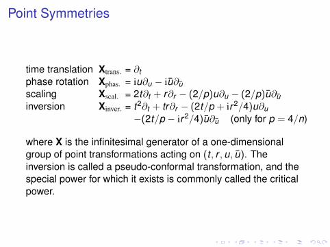
Point Symmetries
time translation Xtrans. = ∂tphase rotation Xphas. = iu∂u − iu∂uscaling Xscal. = 2t∂t + r∂r − (2/p)u∂u − (2/p)u∂uinversion Xinver. = t2∂t + tr∂r − (2t/p + ir2/4)u∂u
−(2t/p − ir2/4)u∂u (only for p = 4/n)
where X is the infinitesimal generator of a one-dimensionalgroup of point transformations acting on (t , r ,u, u). Theinversion is called a pseudo-conformal transformation, and thespecial power for which it exists is commonly called the criticalpower.
Symmetry Groups
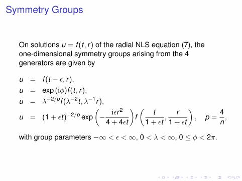
On solutions u = f (t , r) of the radial NLS equation (7), theone-dimensional symmetry groups arising from the 4generators are given by
u = f (t − ε, r),
u = exp (iφ)f (t , r),
u = λ−2/pf (λ−2t , λ−1r),
u = (1 + εt)−2/p exp(− iεr2
4 + 4εt
)f(
t1 + εt
,r
1 + εt
), p =
4n,
with group parameters −∞ < ε <∞, 0 < λ <∞, 0 ≤ φ < 2π.
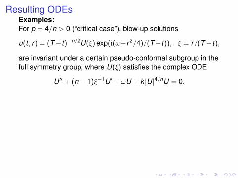
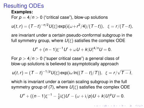
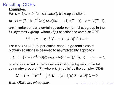
Resulting ODEsExamples:For p = 4/n > 0 (“critical case”), blow-up solutions
u(t , r) = (T−t)−n/2U(ξ) exp(i(ω+r2/4)/(T−t)), ξ = r/(T−t),
are invariant under a certain pseudo-conformal subgroup in thefull symmetry group, where U(ξ) satisfies the complex ODE
U ′′ + (n − 1)ξ−1U ′ + ωU + k |U|4/nU = 0.
For p > 4/n > 0 (“super critical case”) a general class ofblow-up solutions is believed to asymptotically approach
u(t , r) = (T − t)−1/pU(ξ) exp(iω ln((T − t)/T )), ξ = r/√
T − t ,
which is invariant under a certain scaling subgroup in the fullsymmetry group of (7), where U(ξ) satisfies the complex ODE
U ′′ + ((n − 1)ξ−1 − 12 iξ)U ′ − (ω + i/p)U + k |U|pU = 0.
Both ODEs are intractable.
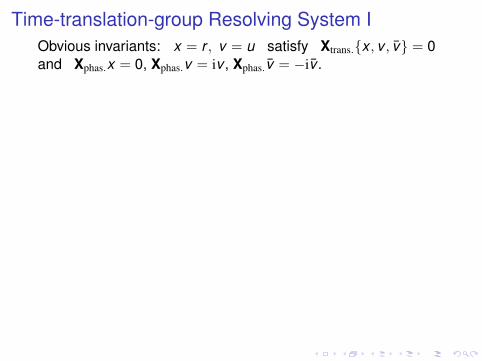
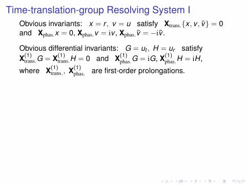
Time-translation-group Resolving System IObvious invariants: x = r , v = u satisfy Xtrans.{x , v , v} = 0and Xphas.x = 0, Xphas.v = iv , Xphas.v = −iv .
Obvious differential invariants: G = ut , H = ur satisfyX(1)
trans.G = X(1)trans.H = 0 and X(1)
phas.G = iG, X(1)phas.H = iH,
where X(1)trans., X(1)
phas. are first-order prolongations.
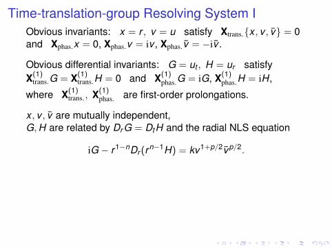
x , v , v are mutually independent,G,H are related by Dr G = DtH and the radial NLS equation
iG − r1−nDr (rn−1H) = kv1+p/2vp/2.
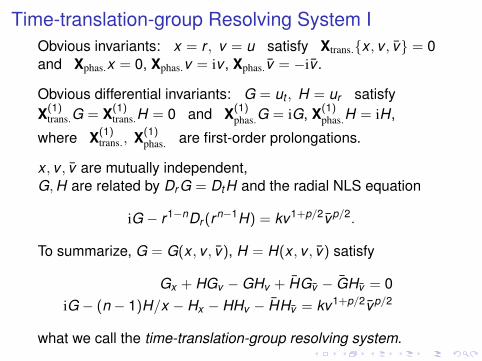
To summarize, G = G(x , v , v), H = H(x , v , v) satisfy
Gx + HGv −GHv + HGv − GHv = 0iG − (n − 1)H/x − Hx − HHv − HHv = kv1+p/2vp/2
what we call the time-translation-group resolving system.
Time-translation-group Resolving System IObvious invariants: x = r , v = u satisfy Xtrans.{x , v , v} = 0and Xphas.x = 0, Xphas.v = iv , Xphas.v = −iv .
Obvious differential invariants: G = ut , H = ur satisfyX(1)
trans.G = X(1)trans.H = 0 and X(1)
phas.G = iG, X(1)phas.H = iH,
where X(1)trans., X(1)
phas. are first-order prolongations.
x , v , v are mutually independent,G,H are related by Dr G = DtH and the radial NLS equation
iG − r1−nDr (rn−1H) = kv1+p/2vp/2.
To summarize, G = G(x , v , v), H = H(x , v , v) satisfy
Gx + HGv −GHv + HGv − GHv = 0iG − (n − 1)H/x − Hx − HHv − HHv = kv1+p/2vp/2
what we call the time-translation-group resolving system.
Time-translation-group Resolving System II
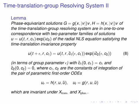
LemmaPhase-equivariant solutions G = g(x , |v |)v ,H = h(x , |v |)v ofthe time-translation-group resolving system are in one-to-onecorrespondence with two-parameter families of solutionsu = u(t , r , c1) exp(ic2) of the radial NLS equation satisfying thetime-translation invariance property
u(t + ε, r , c1) = u(t , r , c1(ε, c1)) exp(ic2(ε, c2)) (8)
(in terms of group parameter ε) with c1(0, c1) = c1 andc2(0, c2) = 0, where c1, c2 are the constants of integration ofthe pair of parametric first-order ODEs
ur = h(r ,u, u), ut = g(r ,u, u)
which are invariant under Xtrans. and Xphas..
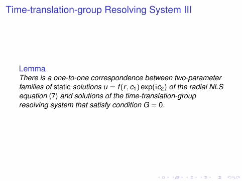
Time-translation-group Resolving System III
LemmaThere is a one-to-one correspondence between two-parameterfamilies of static solutions u = f (r , c1) exp(ic2) of the radial NLSequation (7) and solutions of the time-translation-groupresolving system that satisfy condition G = 0.
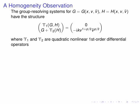
A Homogeneity ObservationThe group-resolving systems for G = G(x , v , v), H = H(x , v , v)have the structure(
Υ1(G,H)G + Υ2(H)
)=
(0
−ikv1+p/2vp/2
)where Υ1 and Υ2 are quadratic nonlinear 1st-order differentialoperators
which obey the homogeneity properties:
Υ1(αv + βvbva, γv + λvbva) = νv + µvbva
Υ2(γv + λvbva) = νv + µvbva + εv2b−1v2a + κva+bva+b−1
with α, β, ε, κ, λ, ν, µ denoting functions only of x .Additionally, these operators have the phase invarianceproperties:
Xphas.Υ1(va+1va, vb+1vb) = iΥ1(va+1va, vb+1vb)
Xphas.Υ2(vb+1vb) = iΥ2(vb+1vb)
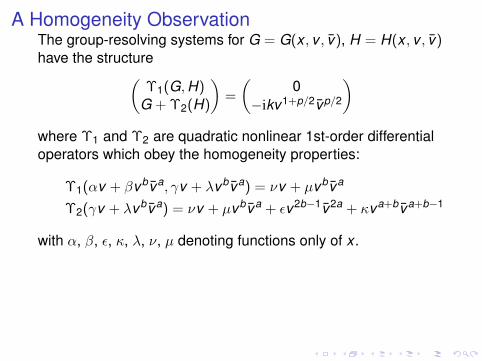
A Homogeneity ObservationThe group-resolving systems for G = G(x , v , v), H = H(x , v , v)have the structure(
Υ1(G,H)G + Υ2(H)
)=
(0
−ikv1+p/2vp/2
)where Υ1 and Υ2 are quadratic nonlinear 1st-order differentialoperators which obey the homogeneity properties:
Υ1(αv + βvbva, γv + λvbva) = νv + µvbva
Υ2(γv + λvbva) = νv + µvbva + εv2b−1v2a + κva+bva+b−1
with α, β, ε, κ, λ, ν, µ denoting functions only of x .
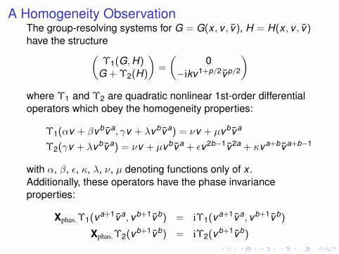
Additionally, these operators have the phase invarianceproperties:
Xphas.Υ1(va+1va, vb+1vb) = iΥ1(va+1va, vb+1vb)
Xphas.Υ2(vb+1vb) = iΥ2(vb+1vb)
A Homogeneity ObservationThe group-resolving systems for G = G(x , v , v), H = H(x , v , v)have the structure(
Υ1(G,H)G + Υ2(H)
)=
(0
−ikv1+p/2vp/2
)where Υ1 and Υ2 are quadratic nonlinear 1st-order differentialoperators which obey the homogeneity properties:
Υ1(αv + βvbva, γv + λvbva) = νv + µvbva
Υ2(γv + λvbva) = νv + µvbva + εv2b−1v2a + κva+bva+b−1
with α, β, ε, κ, λ, ν, µ denoting functions only of x .Additionally, these operators have the phase invarianceproperties:
Xphas.Υ1(va+1va, vb+1vb) = iΥ1(va+1va, vb+1vb)
Xphas.Υ2(vb+1vb) = iΥ2(vb+1vb)
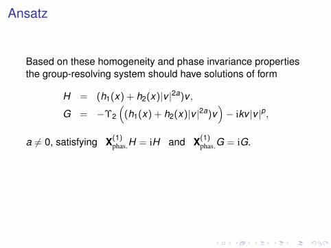
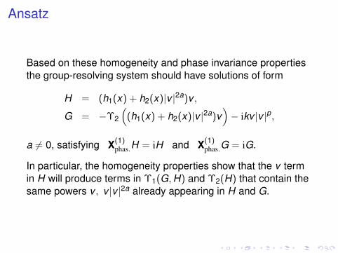
Ansatz
Based on these homogeneity and phase invariance propertiesthe group-resolving system should have solutions of form
H = (h1(x) + h2(x)|v |2a)v ,
G = −Υ2
((h1(x) + h2(x)|v |2a)v
)− ikv |v |p,
a 6= 0, satisfying X(1)phas.H = iH and X(1)
phas.G = iG.
In particular, the homogeneity properties show that the v termin H will produce terms in Υ1(G,H) and Υ2(H) that contain thesame powers v , v |v |2a already appearing in H and G.
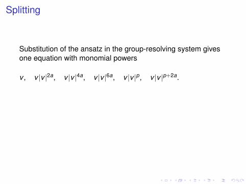
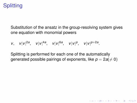
Splitting
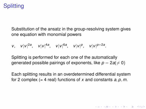
Substitution of the ansatz in the group-resolving system givesone equation with monomial powers
v , v |v |2a, v |v |4a, v |v |6a, v |v |p, v |v |p+2a.
Splitting is performed for each one of the automaticallygenerated possible pairings of exponents, like p = 2a( 6= 0)
Each splitting results in an overdetermined differential systemfor 2 complex (= 4 real) functions of x and constants a,p,m.
Splitting
Substitution of the ansatz in the group-resolving system givesone equation with monomial powers
v , v |v |2a, v |v |4a, v |v |6a, v |v |p, v |v |p+2a.
Splitting is performed for each one of the automaticallygenerated possible pairings of exponents, like p = 2a( 6= 0)
Each splitting results in an overdetermined differential systemfor 2 complex (= 4 real) functions of x and constants a,p,m.
Solution of Overdetermined Systems I
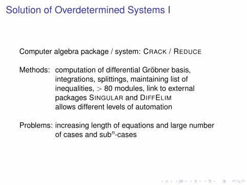
Computer algebra package / system: CRACK / REDUCE
Methods: computation of differential Grobner basis,integrations, splittings, maintaining list ofinequalities, > 80 modules, link to externalpackages SINGULAR and DIFFELIM
allows different levels of automation
Problems: increasing length of equations and large numberof cases and subn-cases
Solution of Overdetermined Systems continued
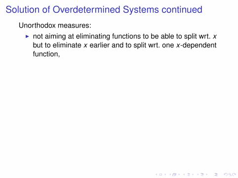
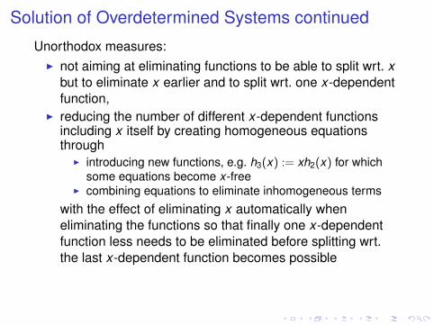
Unorthodox measures:I not aiming at eliminating functions to be able to split wrt. x
but to eliminate x earlier and to split wrt. one x-dependentfunction,
I reducing the number of different x-dependent functionsincluding x itself by creating homogeneous equationsthrough
I introducing new functions, e.g. h3(x) := xh2(x) for whichsome equations become x-free
I combining equations to eliminate inhomogeneous terms
with the effect of eliminating x automatically wheneliminating the functions so that finally one x-dependentfunction less needs to be eliminated before splitting wrt.the last x-dependent function becomes possible
I to work at first only with a subset of equations that arehomogeneous in some sense,
Solution of Overdetermined Systems continued
Unorthodox measures:I not aiming at eliminating functions to be able to split wrt. x
but to eliminate x earlier and to split wrt. one x-dependentfunction,
I reducing the number of different x-dependent functionsincluding x itself by creating homogeneous equationsthrough
I introducing new functions, e.g. h3(x) := xh2(x) for whichsome equations become x-free
I combining equations to eliminate inhomogeneous terms
with the effect of eliminating x automatically wheneliminating the functions so that finally one x-dependentfunction less needs to be eliminated before splitting wrt.the last x-dependent function becomes possible
I to work at first only with a subset of equations that arehomogeneous in some sense,
Solution of Overdetermined Systems continued
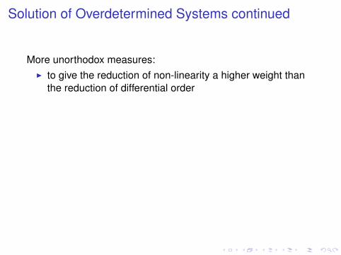
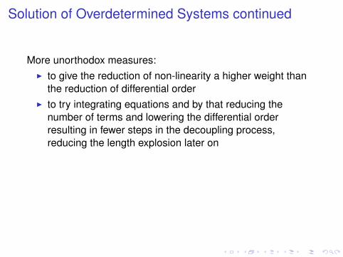
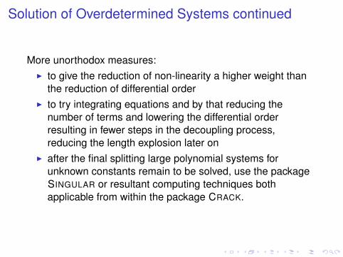
More unorthodox measures:I to give the reduction of non-linearity a higher weight than
the reduction of differential order
I to try integrating equations and by that reducing thenumber of terms and lowering the differential orderresulting in fewer steps in the decoupling process,reducing the length explosion later on
I after the final splitting large polynomial systems forunknown constants remain to be solved, use the packageSINGULAR or resultant computing techniques bothapplicable from within the package CRACK.
Solution of Overdetermined Systems continued
More unorthodox measures:I to give the reduction of non-linearity a higher weight than
the reduction of differential orderI to try integrating equations and by that reducing the
number of terms and lowering the differential orderresulting in fewer steps in the decoupling process,reducing the length explosion later on
I after the final splitting large polynomial systems forunknown constants remain to be solved, use the packageSINGULAR or resultant computing techniques bothapplicable from within the package CRACK.
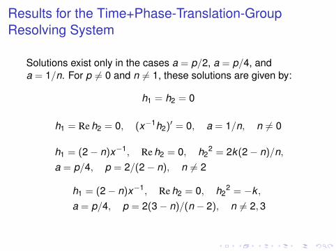
Results for the Time+Phase-Translation-GroupResolving System
Solutions exist only in the cases a = p/2, a = p/4, anda = 1/n. For p 6= 0 and n 6= 1, these solutions are given by:
h1 = h2 = 0
h1 = Re h2 = 0, (x−1h2)′ = 0, a = 1/n, n 6= 0
h1 = (2− n)x−1, Re h2 = 0, h22 = 2k(2− n)/n,
a = p/4, p = 2/(2− n), n 6= 2
h1 = (2− n)x−1, Re h2 = 0, h22 = −k ,
a = p/4, p = 2(3− n)/(n − 2), n 6= 2,3
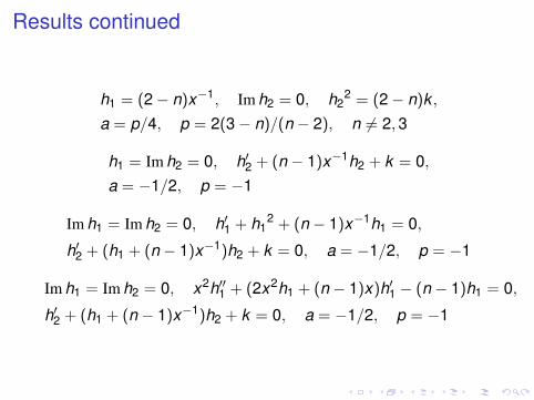
Results continued
h1 = (2− n)x−1, Im h2 = 0, h22 = (2− n)k ,
a = p/4, p = 2(3− n)/(n − 2), n 6= 2,3
h1 = Im h2 = 0, h′2 + (n − 1)x−1h2 + k = 0,a = −1/2, p = −1
Im h1 = Im h2 = 0, h′1 + h12 + (n − 1)x−1h1 = 0,
h′2 + (h1 + (n − 1)x−1)h2 + k = 0, a = −1/2, p = −1
Im h1 = Im h2 = 0, x2h′′1 + (2x2h1 + (n − 1)x)h′1 − (n − 1)h1 = 0,
h′2 + (h1 + (n − 1)x−1)h2 + k = 0, a = −1/2, p = −1
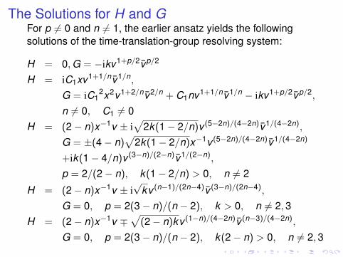
The Solutions for H and GFor p 6= 0 and n 6= 1, the earlier ansatz yields the followingsolutions of the time-translation-group resolving system:
H = 0,G = −ikv1+p/2vp/2
H = iC1xv1+1/nv1/n,
G = iC12x2v1+2/nv2/n + C1nv1+1/nv1/n − ikv1+p/2vp/2,
n 6= 0, C1 6= 0H = (2− n)x−1v ± i
√2k(1− 2/n)v (5−2n)/(4−2n)v1/(4−2n),
G = ±(4− n)√
2k(1− 2/n)x−1v (5−2n)/(4−2n)v1/(4−2n)
+ik(1− 4/n)v (3−n)/(2−n)v1/(2−n),
p = 2/(2− n), k(1− 2/n) > 0, n 6= 2
H = (2− n)x−1v ± i√
kv (n−1)/(2n−4)v (3−n)/(2n−4),
G = 0, p = 2(3− n)/(n − 2), k > 0, n 6= 2,3H = (2− n)x−1v ∓
√(2− n)kv (1−n)/(4−2n)v (n−3)/(4−2n),
G = 0, p = 2(3− n)/(n − 2), k(2− n) > 0, n 6= 2,3
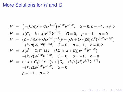
More Solutions for H and G
H =(−(k/n)x + C1x1−n
)v1/2v−1/2, G = 0,p = −1, n 6= 0
H = x(C1 − k ln x)v1/2v−1/2, G = 0, p = −1, n = 0H = (2− n)(x + C1xn−1)−1(v + (C2 + (k/(2n))x2)v1/2v−1/2)
−(k/n)xv1/2v−1/2, G = 0, p = −1, n 6= 0,2H = x(x2 + C1)−1(2v − (kC1 ln x + C2))v1/2v−1/2)
−(k/2)xv1/2v−1/2, G = 0, p = −1, n = 0H = (ln x + C1)−1x−1(v + (C2 + (k/4)x2)v1/2v−1/2)
−(k/2)xv1/2v−1/2, G = 0p = −1, n = 2
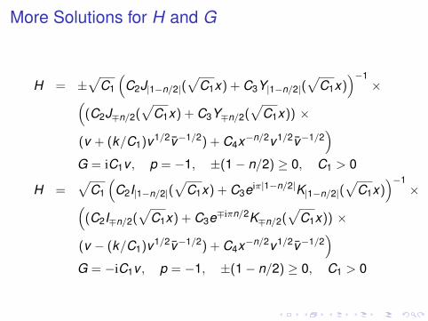
More Solutions for H and G
H = ±√
C1
(C2J|1−n/2|(
√C1x) + C3Y|1−n/2|(
√C1x)
)−1×(
(C2J∓n/2(√
C1x) + C3Y∓n/2(√
C1x)) ×
(v + (k/C1)v1/2v−1/2) + C4x−n/2v1/2v−1/2)
G = iC1v , p = −1, ±(1− n/2) ≥ 0, C1 > 0
H =√
C1
(C2I|1−n/2|(
√C1x) + C3eiπ|1−n/2|K|1−n/2|(
√C1x)
)−1×(
(C2I∓n/2(√
C1x) + C3e∓iπn/2K∓n/2(√
C1x)) ×
(v − (k/C1)v1/2v−1/2) + C4x−n/2v1/2v−1/2)
G = −iC1v , p = −1, ±(1− n/2) ≥ 0, C1 > 0
Solutions of the Radial NLS
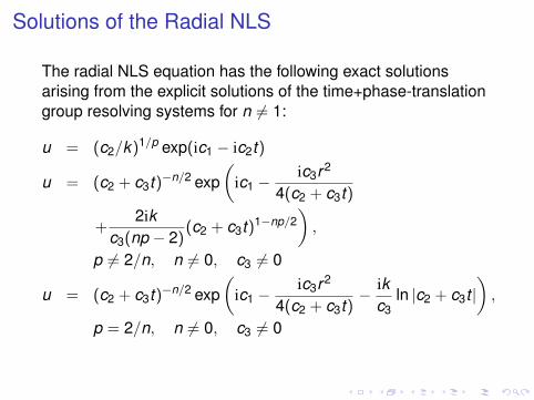
The radial NLS equation has the following exact solutionsarising from the explicit solutions of the time+phase-translationgroup resolving systems for n 6= 1:
u = (c2/k)1/p exp(ic1 − ic2t)
u = (c2 + c3t)−n/2 exp(
ic1 −ic3r2
4(c2 + c3t)
+2ik
c3(np − 2)(c2 + c3t)1−np/2
),
p 6= 2/n, n 6= 0, c3 6= 0
u = (c2 + c3t)−n/2 exp(
ic1 −ic3r2
4(c2 + c3t)− ik
c3ln |c2 + c3t |
),
p = 2/n, n 6= 0, c3 6= 0
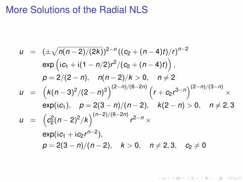
More Solutions of the Radial NLS
u = (±√
n(n − 2)/(2k))2−n ((c2 + (n − 4)t)/r)n−2
exp(
ic1 + i(1− n/2)r2/(c2 + (n − 4)t)),
p = 2/(2− n), n(n − 2)/k > 0, n 6= 2
u =(
k(n − 3)2/(2− n)3)(2−n)/(6−2n) (
r + c2r3−n)(2−n)/(3−n)
×
exp(ic1), p = 2(3− n)/(n − 2), k(2− n) > 0, n 6= 2,3
u =(
c22(n − 2)2/k
)(n−2)/(6−2n)r2−n ×
exp(ic1 + ic2rn−2),
p = 2(3− n)/(n − 2), k > 0, n 6= 2,3, c2 6= 0
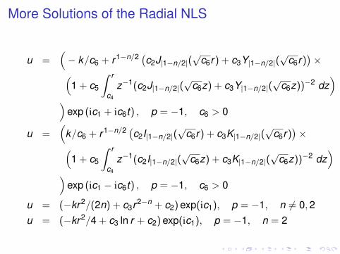
More Solutions of the Radial NLS
u =(− k/c6 + r1−n/2 (c2J|1−n/2|(
√c6r) + c3Y|1−n/2|(
√c6r)
)×(
1 + c5
∫ r
c4
z−1(c2J|1−n/2|(√
c6z) + c3Y|1−n/2|(√
c6z))−2 dz)
)exp (ic1 + ic6t) , p = −1, c6 > 0
u =(
k/c6 + r1−n/2 (c2I|1−n/2|(√
c6r) + c3K|1−n/2|(√
c6r))×(
1 + c5
∫ r
c4
z−1(c2I|1−n/2|(√
c6z) + c3K|1−n/2|(√
c6z))−2 dz)
)exp (ic1 − ic6t) , p = −1, c6 > 0
u = (−kr2/(2n) + c3r2−n + c2) exp(ic1), p = −1, n 6= 0,2u = (−kr2/4 + c3 ln r + c2) exp(ic1), p = −1, n = 2
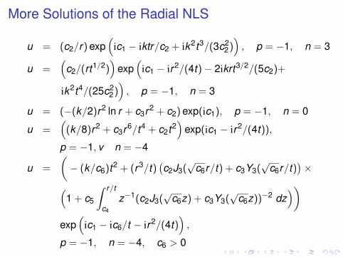
More Solutions of the Radial NLS
u = (c2/r) exp(
ic1 − iktr/c2 + ik2t3/(3c22)), p = −1, n = 3
u =(
c2/(rt1/2))
exp(
ic1 − ir2/(4t)− 2ikrt3/2/(5c2)+
ik2t4/(25c22)), p = −1, n = 3
u = (−(k/2)r2 ln r + c3r2 + c2) exp(ic1), p = −1, n = 0
u =(
(k/8)r2 + c3r6/t4 + c2t2)
exp(ic1 − ir2/(4t)),
p = −1, v n = −4
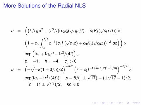
u =
(− (k/c6)t2 + (r3/t)
(c2J3(
√c6r/t) + c3Y3(
√c6r/t)
)×(
1 + c5
∫ r/t
c4
z−1(c2J3(√
c6z) + c3Y3(√
c6z))−2 dz))
exp(
ic1 − ic6/t − ir2/(4t)),
p = −1, n = −4, c6 > 0
More Solutions of the Radial NLS
u =
((k/c6)t2 + (r3/t)(c2I3(
√c6r/t) + c3K3(
√c6r/t))×(
1 + c5
∫ r/t
c4
z−1(c2I3(√
c6z) + c3K3(√
c6z))−2 dz))×
exp(
ic1 + ic6/t − ir2/(4t)),
p = −1, n = −4, c6 > 0
u =(±√−k(1 + 3/n)/2
)−n/2 (r + c2t−1+4/nr2(1−2/n)
)−n/2×
exp(ic1 − ir2/(4t)), p = 8/(1±√
17) = (±√
17− 1)/2,n = (1±
√17)/2, kn < 0
More Solutions of the Radial NLS
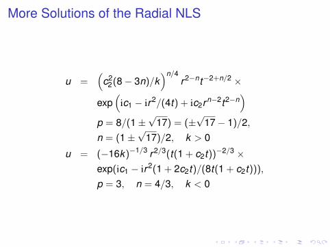
u =(
c22(8− 3n)/k
)n/4r2−nt−2+n/2 ×
exp(
ic1 − ir2/(4t) + ic2rn−2t2−n)
p = 8/(1±√
17) = (±√
17− 1)/2,n = (1±
√17)/2, k > 0
u = (−16k)−1/3 r2/3(t(1 + c2t))−2/3 ×exp(ic1 − ir2(1 + 2c2t)/(8t(1 + c2t))),
p = 3, n = 4/3, k < 0

Outline
Introduction
Group Foliation in 5 Steps
Solving the Group-Resolving System
Solutions for the Nonlinear Heat Equation
The semilinear radial Schrodinger equations
Summary
Summary
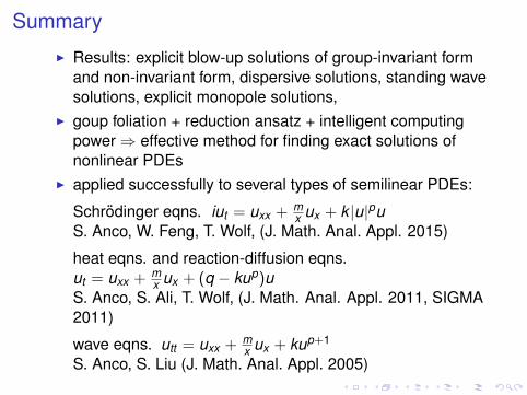
I Results: explicit blow-up solutions of group-invariant formand non-invariant form, dispersive solutions, standing wavesolutions, explicit monopole solutions,
I goup foliation + reduction ansatz + intelligent computingpower⇒ effective method for finding exact solutions ofnonlinear PDEs
I applied successfully to several types of semilinear PDEs:
Schrodinger eqns. iut = uxx + mx ux + k |u|pu
S. Anco, W. Feng, T. Wolf, (J. Math. Anal. Appl. 2015)
heat eqns. and reaction-diffusion eqns.ut = uxx + m
x ux + (q − kup)uS. Anco, S. Ali, T. Wolf, (J. Math. Anal. Appl. 2011, SIGMA2011)
wave eqns. utt = uxx + mx ux + kup+1
S. Anco, S. Liu (J. Math. Anal. Appl. 2005)
Summary
I Results: explicit blow-up solutions of group-invariant formand non-invariant form, dispersive solutions, standing wavesolutions, explicit monopole solutions,
I goup foliation + reduction ansatz + intelligent computingpower⇒ effective method for finding exact solutions ofnonlinear PDEs
I applied successfully to several types of semilinear PDEs:
Schrodinger eqns. iut = uxx + mx ux + k |u|pu
S. Anco, W. Feng, T. Wolf, (J. Math. Anal. Appl. 2015)
heat eqns. and reaction-diffusion eqns.ut = uxx + m
x ux + (q − kup)uS. Anco, S. Ali, T. Wolf, (J. Math. Anal. Appl. 2011, SIGMA2011)
wave eqns. utt = uxx + mx ux + kup+1
S. Anco, S. Liu (J. Math. Anal. Appl. 2005)
Future Work
Application to other types of PDEs, e.g. ≥ 3 independentvariables, quasilinear, derivative nonlinearities, larger numberof symmetries

The End
Thank you!