Embed Size (px)
Citation preview

Journal of Applied Statistical ScienceVolume 16, Number 4, pp. 23–35
ISSN 1067-5817c© 2008 Nova Science Publishers, Inc.
EXACT PROPERTIES OF A NEW TEST AND OTHERTESTS FOR DIFFERENCES BETWEEN SEVERAL
BINOMIAL PROPORTIONS
K. Krishnamoorthy∗Department of Mathematics
University of Louisiana at LafayetteLafayette, LA 70504
Jie Peng†
Department of Finance, Economics and Decision ScienceSt. Ambrose UniversityDavenport, Iowa 52803
Abstract
The problem of testing equality of several binomial proportions is considered. An approxi-mate unconditional test (AU-test) is proposed by extending a method for the two-sample case.Exact binomial distributions are used to evaluate Type I error rates of the usual chi-square test,an exact conditional test, a conditional test based on mid p-value and the AU-test numerically.The AU-test and the conditional test based on mid p-values control the Type I error rates verysatisfactorily even for small samples whereas the exact conditional test is too conservative.The powers of the chi-square test, conditional test based on mid-p value, and the AU-test areevaluated and compared. Power comparison shows that all three tests exhibit similar powerproperties when their sizes are within the nominal level. The AU-test practically behaves likean exact test even for small samples, and can be safely used for applications. The results areillustrated using an example where small proportions are to be compared.
Key Words and Phrases: Conditional exact test; Mid-p value; Parametric bootstrap; Powers; Size
1. Introduction
The problem of testing equality of two proportions is well addressed in the literature. Numerousarticles have been written on this topic proposing several approximate and exact tests. Amongthe available methods, Fisher’s conditional test (conditional on the total number of successes) hasbeen a popular choice because of its simplicity and guarantee that the Type I error rates neverexceed the nominal level. This test, however, is overly conservative when the sample sizes are smalland/or the proportions are at the boundaries. For these reasons, exact unconditional proceduresgained popularity among researchers as they are usually less discrete and more powerful than theconditional test. Barnard (1945, 1947) developed an unconditional test by maximizing the p-valuewith respect to the common unknown parameter under the null hypothesis of equality of proportions.
∗E-mail address: [email protected]; Tel. 337 482 5283; Fax 337 482 5346 (Corresponding Author)†E-mail address: [email protected]

24 K. Krishnamoorthy and Jie Peng
This unconditional test is also subject to criticism because it is computationally very intensive, andis also conservative. Several articles addressed the two-sample problem and extensive comparisonstudies were carried out by many authors. For example, see Upton (1982), Haber (1986), Storer andKim (1990), Berger (1996), Martin and Silva (1994) and Martin et al. (1998, 2002) and Chan andZhang (1999) and the references therein.
The problem of comparing several proportions arises when we have samples from m popula-tions (lots of items, opinions of serval groups of people on a public issue, products from differentsuppliers, etc.), and want to test whether there are significant differences in the proportions for thesepopulations. This problem is also well-known, and has been discussed in many text books (e.g.,Scheaffer and McClave 1994 and Zar 1999). However, unlike the two-sample case, only very lim-ited results are available. Williams (1988) pointed out a practical situation where small proportionsare to be compared, and proposed conditional tests (conditionally given the total number of suc-cesses from all samples) based on several statistics appropriate for different alternative hypothesessuch as p1 ≥ pi, i = 2, ...,m or p1 ≤ p2 ≤ ... ≤ p j ≥ p j+1 ≥ ... ≥ pm ≥ p1 for some j, 1 ≤ j ≤ m.Williams also studied conditional Type I error rates of the proposed tests.
To describe the problem formally, consider m independent binomial random variablesX1, ...,Xm with Xi ∼ binomial(ni, pi), 0 < pi < 1, i = 1, ...,m. Let ki be an observed value of Xi,i = 1, ...,m. The hypotheses of interest are
H0 : p1 = ... = pm vs. Ha : pi 6= p j for some i 6= j. (1)
Kulkarni and Shah (1995) and Krishnamoorthy et al. (2004) considered the above problem whenthe common proportion under H0 is specified. Specifically, Krishnamoorthy et al. proposed asimple exact method for hypothesis testing. If the common proportion is unspecified, then the χ2
approximate test is commonly used. The χ2-test is based on the statistic
Qx =m
∑i=1
ni(p̂xi− p̂x)2
p̂x(1− p̂x), (2)
where p̂xi = Xini
, i = 1, ...,m and p̂x = ∑mi=1 Xi
∑mi=1 ni
. Under H0, Qx follows a χ2m−1 distribution approximately.
Notice that, for the case of m = 2, the statistic Qx is the squared Z-test statistic
p̂x1− p̂x2√p̂x(1− p̂x)
(1n1
+ 1n2
)
for comparing two proportions. For this case, Storer and Kim (1990) showed that the χ2 test is oftenliberal especially when sample sizes are quite different.
In this article, we study unconditional Type I error rates of the usual chi-square test, the con-ditional test, the conditional test based on mid-p value, and a new test. Specifically, the Type Ierror rates and powers are evaluated using the exact binomial distributions not normal or chi-squareapproximations. The new test is obtained by extending an approximate unconditional test (AU-test)first considered in Storer and Kim (1990), later by Krishnamoorthy and Thomson (2002) for thefinite population case and Krishnamoorthy and Thomson (2004) for the Poisson case. Even thoughthere are several alternative tests are available for the two-sample case, not all of them can be easilyextended to the present problem of comparing several proportions, except the AU-test. Storer andKim (1990) and Krishnamoorthy and Thomson (2002, 2004) found that the AU-test performed verysatisfactorily even for small samples. As the AU-test is actually based on an estimated p-value,Krishnamoorthy and Thomson (2002, 2004) referred to it as the E-test.
Exact Properties of a New Test and Other Tests... 25
In view of the above motivation and discussion, this article is organized as follows. In thefollowing section, we outline the χ2-test, the conditional tests and the AU-test. The likelihoodratio test (LRT) for comparing proportions in a multinomial setup (Cai and Krishnamoorthy 2006)exhibited poor size properties and usually inferior to the χ2-test. Our preliminary numerical studiesin the present setup showed the LRT is in general inferior to the χ2-test, and so we will not includethe LRT here for comparisons. An exact method of calculating size and power of a test is givenin Section 3. Using this method, the sizes of the tests are evaluated for m = 3 and 4. Powers arealso evaluated for a few parameter and sample size configurations. The size and power studiesshow that the AU-test followed by the conditional test based on mid-p value are very satisfactoryeven for small samples. The Type I error rates of the AU-test seldom exceed the nominal levelby a negligible amount, and perform almost like an exact test. The results are illustrated using anexample in Section 4. Some concluding remarks are given in Section 5.
2. The Tests
Let (k1, ...,km) be an observed value of (X1, ...,Xm), and Qk be an observed value of Qx
in (2). That is,
Qk =m
∑i=1
ni(p̂ki− p̂k)2
p̂k(1− p̂k), (3)
where p̂ki = kini
, i = 1, ...,m and p̂k = ∑mi=1 ki
∑mi=1 ni
is the pooled estimate of the common unknown propor-tion.
2.1. The χ2-test
For a given level α, the χ2-test rejects the null hypothesis in (1) if Qk is greater than or equal to thecritical value χ2
m−1,α, where χ2a,α denotes the upper α quantile of the χ2
a distribution. Equivalently,it rejects the null hypothesis if P(χ2
m−1 ≥ Qk|H0)≤ α.
2.2. Conditional Tests
An exact conditional test can be developed using the conditional joint distribution of X1, ...,Xm giventhat ∑m
i=1 Xi = x and p1 = ... = pm. This conditional distribution is multivariate hypergeometric withthe probability mass function given by
P
(X1 = x1, ...,Xm = xm
∣∣∣∣m
∑i=1
Xi = x
)=
(n1x1
)(n2x2
) · · ·(nmxm
)(n
x
) , (4)
where n = n1 + ...+nm and x = x1 + ...+ xm.
The C-test
If we use the Qx as a test statistic, then the exact conditional p-value can be computed using theexpression
P
(Qx ≥ Qk
∣∣∣∣m
∑i=1
Xi = x
)=
u1
∑x1=l1
...um−1
∑xm−1=lm−1
(n1x1
)(n2x2
) · · ·(nmxm
)(n
x
) I (Qx ≥ Qk) , (5)

26 K. Krishnamoorthy and Jie Peng
where Qk is an observed value of Qx, I(.) is the indicator function and, for i = 1, ...,m−1,
li = max
{0,x−
i−1
∑j=1
x j−k
∑j=i+1
n j
}, ui = min
{ni,x−
i−1
∑j=1
x j
}(6)
and
um = min
{nm,x−
m−1
∑j=1
x j
}.
Notice that we have used m−1 sums in (5), because x1 + ...+ xm = x. One could use any other teststatistic in place of Qx depending on the alternative hypothesis. As pointed out by Williams (1988),the statistic Qx given in (2) is appropriate for the general alternative hypothesis in (1). We refer tothis test as the C-test.
CM-test
Some authors suggested using mid-p values for hypothesis tests involving discrete distributions.A mid-p value for the above conditional test can be computed as
12
[P
(Qx ≥ Qk
∣∣∣∣m
∑i=1
Xi = x
)+P
(Qx > Qk
∣∣∣∣m
∑i=1
Xi = x
)].
The null hypothesis in (1) will be rejected whenever this mid-p value is less than or equal to thenominal level α. As the conditional tests are usually very conservative, the use of mid-p valueapproach will reduce the conservatism. Williams (1988) preferred the mid-p value approach on thebasis of arguments favoring the use of mid-p values given in Lancaster (1961), Anscombe (1981)and Frank (1986). Furthermore, for the two-sample case, Martin et al. (1998) compared severaltests, and concluded that Fisher’s conditional test based on mid-p value is preferable to others forsimplicity and power.
2.3. The AU-test
If the common proportion under H0 is specified as p0, then the p-value of the statistic Qx can becomputed using the expression
n1
∑x1=0
...nm
∑xm=0
(m
∏i=1
f (xi;ni, p0)
)I (Qx ≥ Qk) , (7)
where
f (x;n, p) =(
nx
)px(1− p)n−x, x = 0,1, . . . ,n, 0 < p < 1,
is the binomial probability mass function. The test based on the p-value in (7) is exact in the sensethat the Type I error rates are always within the nominal level. The common proportion is usuallyunknown, and in this case the unconditional p-value can be obtained as
sup0<p<1
n1
∑x1=0
...nm
∑xm=0
(m
∏i=1
f (xi;ni, p)
)I (Qx ≥ Qk) . (8)

Exact Properties of a New Test and Other Tests... 27
The test based on the above p-value is an exact unconditional test which is an extension of Barnard’sunconditional test for the two-sample case. As pointed out earlier, this test is computationally in-tensive even for m = 2. As an alternative, Storer and Kim (1990) proposed an approximate uncon-ditional test (AU-test) on the basis of the p-value evaluated at the maximum likelihood estimator ofp. That is, p-value is computed as
n1
∑x1=0
...nm
∑xm=0
(m
∏i=1
f (xi;ni, p̂k)
)I (Qx ≥ Qk) , (9)
where p̂k is as defined in (3). As the p-value is evaluated only at p̂k, it is easier to compute thanthe p-value in (8). As the test is based on an estimated p-value, Krishnamoorthy and Thomson(2002,2004) referred to this test as the E-test. This AU-test should be used with the convention ofnot rejecting the null hypothesis in extreme cases where (k1, ...,km) = (0, ...,0) or (n1, ...,nm).
Even though the p-value is calculated only at p̂k, calculation is quite time consuming if m and/orsample sizes are large. An alternative simple approach of computing the p-value in (9) is on the basisof an observation by Krishnamoorthy and Thomson (2002). These authors noted that the AU-test (inthe context of comparing two proportions in finite populations) is essentially equivalent to the onebased on the parametric bootstrap (PB) approach (see Krishnamoorthy and Thomson 2002, Remark2). In other words, the AU-test described above can be regarded as the PB method using exactbinomial distribution rather than simulation. Thus, the p-value in (9) can be computed using the PBapproach given in the following algorithm.
Algorithm 1For a given (n1, ...,nm) and (k1, ...,km):compute the sample proportion p̂ki = ki
ni, i = 1, ...,m and
the pooled sample proportion p̂k = ∑mi=1 ki
∑mi=1 ni
compute the observed statistic Qk = ∑mi=1
ni(p̂ki−p̂k)2
p̂k(1−p̂k)set T = 0For i = 1 to N
generate x j ∼ binomial(n j, p̂k), j = 1, ...,m
compute p̂x j = x jn j
, j = 1, ...,m and p̂x = ∑mj=1 x j
∑mj=1 n j
compute Qx = ∑mj=1
n j(p̂x j−p̂x)2
p̂x(1−p̂x)if Qx ≥ Qk, set T = T +1
(end do loop)TN is the PB p-value that should be close to the one in (9) if N is large enough.
2.4. Comparison of P-values
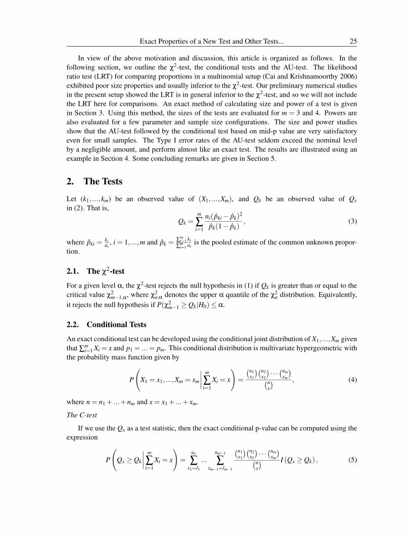
We computed the p-values of all four tests when m = 4 and presented them in Table 1. The values of(n1, ...,n4) and (k1, ...,k4) were chosen arbitrarily. To judge the accuracies of the PB test based onAlgorithm 1, we computed its p-values and presented them in Table 1 along with the exact p-valuesof the AU-test based on (9). We see from Table 1 that these p-values are practically the same for allthe cases considered. Thus, for large m and/or moderate to large sample sizes one can use Algorithm1 to compute the p-value of the AU-test. As expected, the p-values of the C-test are always greaterthan or equal to the corresponding p-values of the CM-test. The p-values of the χ2-test are thesmallest in many cases, especially when the sample sizes are small or the sample sizes are muchdifferent.
28 K. Krishnamoorthy and Jie Peng
Table 1. Comparison of p-values of (a) χ2-test, (b) C-test, (c) CM-test, (d) AU-test (9) and (e)PB Algorithm 1 with N = 100,000 runs
Sample Sizes No. of Successes Observed p-values(n1, ...,n4) (k1, ...,k4) Statistic Qk a b c d e(4, 4, 4, 4) (4, 4, 1, 1) 9.600 .022 .045 .033 .019 .019(5, 9, 3,12) (4, 3, 2, 9) 4.719 .194 .207 .203 .207 .205
(32, 5,10,12) (16, 4, 4, 4) 3.390 .335 .374 .372 .352 .351(10,10,10,10) (9, 5, 5, 9) 7.619 .055 .053 .050 .048 .048(25, 5, 5, 5) (20, 4, 3, 1) 7.619 .055 .056 .049 .052 .052
(13,12,11, 4) (4, 4, 4, 4) 6.744 .081 .085 .085 .079 .078(23, 4, 4, 4) (16, 3, 2, 1) 3.435 .329 .377 .329 .329 .330
(40,40,40,40) (12, 9, 6, 3) 7.385 .061 .065 .061 .061 .062(3, 3, 3, 3) (3, 3, 1, 1) 6.000 .112 .182 .127 .143 .143(5, 5, 5, 5) (5, 2, 1, 1) 8.687 .034 .041 .033 .028 .027
(12,23,45,60) (4, 9,23,36) 4.732 .192 .193 .193 .196 .196(5, 4, 8, 9) (5, 3, 3, 7) 6.375 .095 .097 .092 .091 .091
(32, 4, 4, 4) (16, 4, 3, 3) 4.701 .195 .247 .243 .236 .238
3. Size and Power Studies of the Tests
The exact size or power of the χ2-test can be computed using the expression
n1
∑k1=0
...nm
∑km=0
(m
∏i=1
f (ki;ni, pi)
)I(P(χ2
m−1 ≥ Qk)≤ α). (10)
Notice that the above expression gives Type I error rate when p1 = ... = pm and power otherwise.The exact size and power of the other tests can be computed using the expression
n1
∑k1=0
...nm
∑km=0
(m
∏i=1
f (ki;ni, pi)
)I (p-value≤ α) . (11)
For example, to compute the size or power of the AU-test, use the p-value given in (9).
3.1. Size Properties
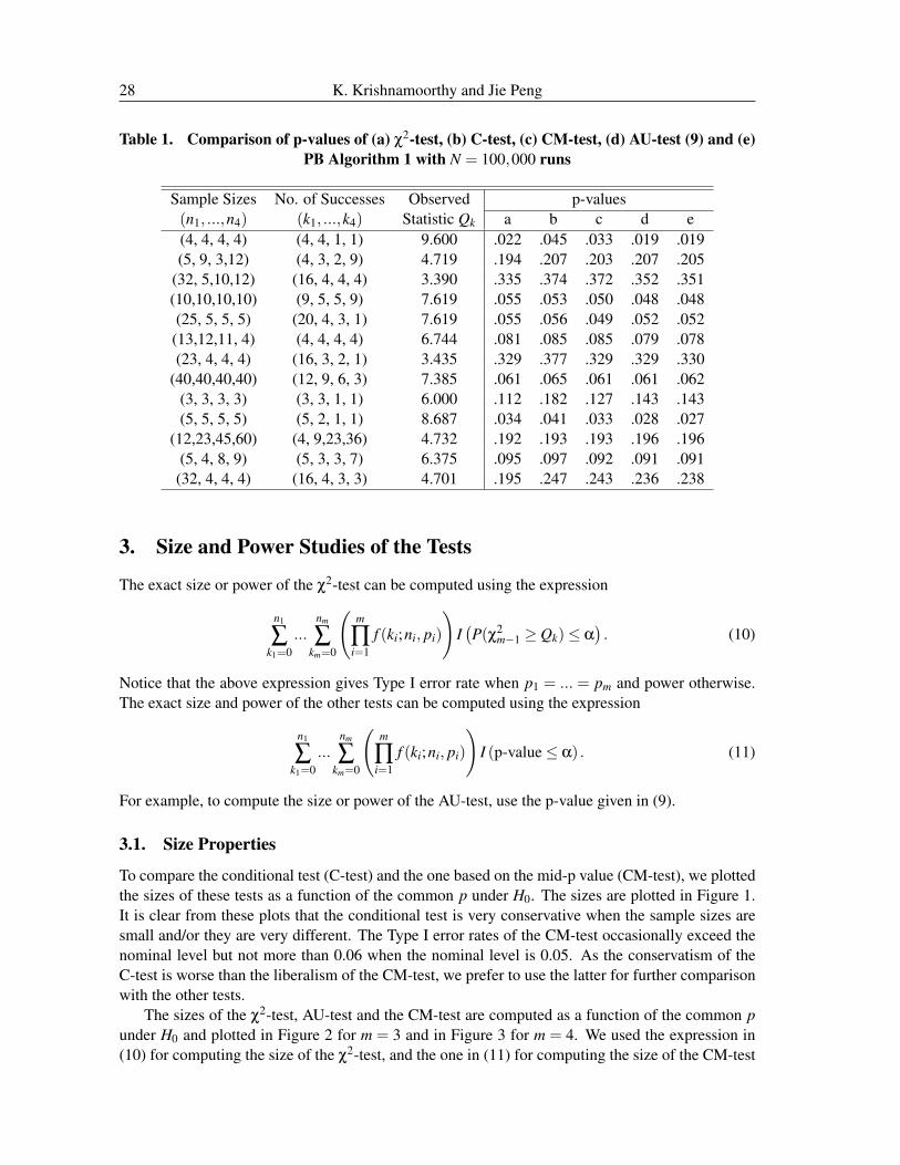
To compare the conditional test (C-test) and the one based on the mid-p value (CM-test), we plottedthe sizes of these tests as a function of the common p under H0. The sizes are plotted in Figure 1.It is clear from these plots that the conditional test is very conservative when the sample sizes aresmall and/or they are very different. The Type I error rates of the CM-test occasionally exceed thenominal level but not more than 0.06 when the nominal level is 0.05. As the conservatism of theC-test is worse than the liberalism of the CM-test, we prefer to use the latter for further comparisonwith the other tests.
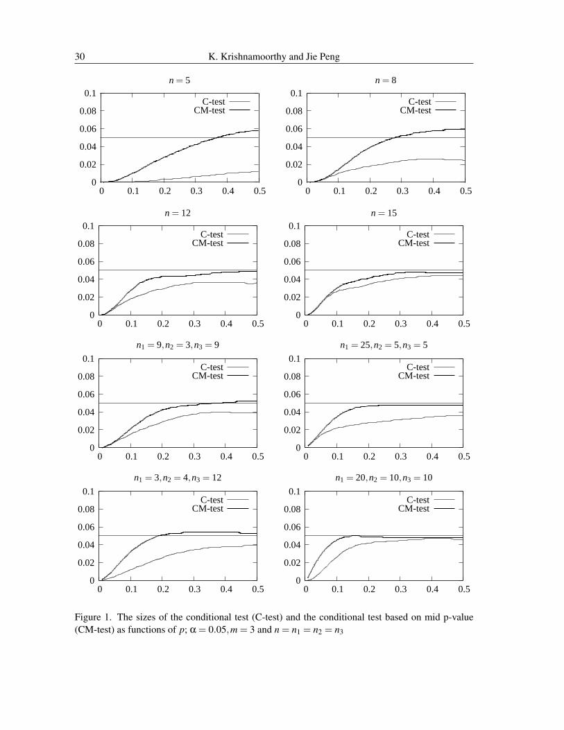
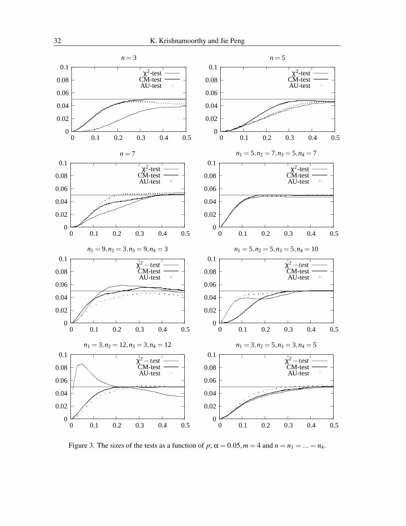
The sizes of the χ2-test, AU-test and the CM-test are computed as a function of the common punder H0 and plotted in Figure 2 for m = 3 and in Figure 3 for m = 4. We used the expression in(10) for computing the size of the χ2-test, and the one in (11) for computing the size of the CM-test

Exact Properties of a New Test and Other Tests... 29
and the AU-test. As we are interested in small-sample properties of the tests, we did not includelarge samples. We observe the following from Figures 2 and 3.
1. The sizes of the χ2-test exceed the nominal level quite often. In particular, when n1 = 25,n2 =5,n = 5, the size of the χ2-test exceeds 0.3 when the nominal level is 0.05. This implies thatthere are situations where the χ2-test could be too liberal. Even though the χ2-test is stillliberal for the case of m = 4 (Figure 3), it exhibits slightly better performance than it did forthe case of m = 3.
2. The CM-test offers improvement over the χ2-test in controlling sizes. This test is slightlyliberal when some sample sizes are very different.
3. It is clear from Figures 2 and 3 that the AU-test controls the Type I error rates very wellregardless of sample sizes except in two cases (Figure 2, n1 = n2 = n3 = 12 and Figure 3,n = 7) where its Type I error rates barely exceed the nominal level.
The χ2-test, in general, performs satisfactorily if sample sizes are not very small and/or drasti-cally different. It appears that the liberalism of the test diminishes with increasing m. The CM-testoffers improvement over the χ2-test, but it is computationally intensive for m ≥ 4 and/or the ob-served number of successes are large. Over all, the AU-test performs very satisfactorily and behavesalmost like an exact test; it can be safely used for applications regardless of sample sizes.
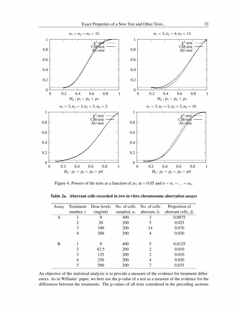
3.2. Power Properties
In general, it is fair to compare two tests with respect to powers only if they are level α tests.Therefore, for power comparison studies we chose the situations where all three tests control theType I error rates within the nominal level. The powers are plotted (alternative hypotheses arespecified below the plots) in Figure 4. It is clear from these plots that only little differences existbetween the powers. No test dominates the others uniformly except in one case where n1 = 5,n2 =5,n3 = 5,n4 = 10; in this exceptional case, we observe from Figure 4 that the sizes of the AU-testand the CM-test are greater than or equal to (but within the nominal level) those of the χ2-test, andas a result, they provide slightly more powers than the χ2-test.
4. An Example
This example is taken from Williams (1988) and the results are outcomes of a chromosome aber-ration assay study to determine whether or not the compound is clastogenic. The purpose of thisstudy is to assess the toxicity of compounds such as drugs, food additives and pesticides. The datafor two assays A and B from Table 1 of Williams (1988) are reproduced here in Table 2a.
30 K. Krishnamoorthy and Jie Peng
0
0.02
0.04
0.06
0.08
0.1
0 0.1 0.2 0.3 0.4 0.5
n = 5
C-testCM-test
0
0.02
0.04
0.06
0.08
0.1
0 0.1 0.2 0.3 0.4 0.5
n = 8
C-testCM-test
0
0.02
0.04
0.06
0.08
0.1
0 0.1 0.2 0.3 0.4 0.5
n = 12
C-testCM-test
0
0.02
0.04
0.06
0.08
0.1
0 0.1 0.2 0.3 0.4 0.5
n = 15
C-testCM-test
0
0.02
0.04
0.06
0.08
0.1
0 0.1 0.2 0.3 0.4 0.5
n1 = 9,n2 = 3,n3 = 9
C-testCM-test
0
0.02
0.04
0.06
0.08
0.1
0 0.1 0.2 0.3 0.4 0.5
n1 = 25,n2 = 5,n3 = 5
C-testCM-test
0
0.02
0.04
0.06
0.08
0.1
0 0.1 0.2 0.3 0.4 0.5
n1 = 3,n2 = 4,n3 = 12
C-testCM-test
0
0.02
0.04
0.06
0.08
0.1
0 0.1 0.2 0.3 0.4 0.5
n1 = 20,n2 = 10,n3 = 10
C-testCM-test
Figure 1. The sizes of the conditional test (C-test) and the conditional test based on mid p-value(CM-test) as functions of p; α = 0.05,m = 3 and n = n1 = n2 = n3
Exact Properties of a New Test and Other Tests... 31
0
0.02
0.04
0.06
0.08
0.1
0 0.1 0.2 0.3 0.4 0.5
n = 5
χ2-testCM-testAU-test
0
0.02
0.04
0.06
0.08
0.1
0 0.1 0.2 0.3 0.4 0.5
n = 8
χ2-testCM-testAU-test
0
0.02
0.04
0.06
0.08
0.1
0 0.1 0.2 0.3 0.4 0.5
n = 12
χ2-testCM-testAU-test
0
0.02
0.04
0.06
0.08
0.1
0 0.1 0.2 0.3 0.4 0.5
n = 15
χ2-testCM-testAU-test
0
0.02
0.04
0.06
0.08
0.1
0 0.1 0.2 0.3 0.4 0.5
n1 = 9,n2 = 3,n3 = 9
χ2-testCM-testAU-test
0
0.05
0.1
0.15
0.2
0.25
0.3
0 0.1 0.2 0.3 0.4 0.5
n1 = 25,n2 = 5,n3 = 5
χ2-testCM-testAU-test
0
0.02
0.04
0.06
0.08
0.1
0 0.1 0.2 0.3 0.4 0.5
n1 = 3,n2 = 4,n3 = 12
χ2-testCM-testAU-test
0
0.02
0.04
0.06
0.08
0.1
0 0.1 0.2 0.3 0.4 0.5
n1 = 20,n2 = 10,n3 = 10
χ2-testCM-testAU-test
Figure 2. The sizes of the tests as functions of p; α = 0.05,m = 3 and n = n1 = n2 = n3.
32 K. Krishnamoorthy and Jie Peng
0
0.02
0.04
0.06
0.08
0.1
0 0.1 0.2 0.3 0.4 0.5
n = 3
χ2-testCM-testAU-test
0
0.02
0.04
0.06
0.08
0.1
0 0.1 0.2 0.3 0.4 0.5
n = 5
χ2-testCM-testAU-test
0
0.02
0.04
0.06
0.08
0.1
0 0.1 0.2 0.3 0.4 0.5
n = 7
χ2-testCM-testAU-test
0
0.02
0.04
0.06
0.08
0.1
0 0.1 0.2 0.3 0.4 0.5
n1 = 5,n2 = 7,n3 = 5,n4 = 7
χ2-testCM-testAU-test
0
0.02
0.04
0.06
0.08
0.1
0 0.1 0.2 0.3 0.4 0.5
n1 = 9,n2 = 3,n3 = 9,n4 = 3
χ2− test
CM-testAU-test
0
0.02
0.04
0.06
0.08
0.1
0 0.1 0.2 0.3 0.4 0.5
n1 = 5,n2 = 5,n3 = 5,n4 = 10
χ2− test
CM-testAU-test
0
0.02
0.04
0.06
0.08
0.1
0 0.1 0.2 0.3 0.4 0.5
n1 = 3,n2 = 12,n3 = 3,n4 = 12
χ2− test
CM-testAU-test
0
0.02
0.04
0.06
0.08
0.1
0 0.1 0.2 0.3 0.4 0.5
n1 = 3,n2 = 5,n3 = 3,n4 = 5
χ2− test
CM-testAU-test
Figure 3. The sizes of the tests as a function of p; α = 0.05,m = 4 and n = n1 = ... = n4.
Exact Properties of a New Test and Other Tests... 33
0
0.2
0.4
0.6
0.8
1
0 0.2 0.4 0.6 0.8 1Ha : p1 = p2 < p3
n1 = n2 = n3 = 15
χ2-testCM-testAU-test
0
0.2
0.4
0.6
0.8
1
0 0.2 0.4 0.6 0.8 1Ha : p1 = p2 < p3
n1 = 3,n2 = 4,n3 = 13
χ2-testCM-testAU-test
0
0.2
0.4
0.6
0.8
1
0 0.2 0.4 0.6 0.8 1Ha : p1 = p2 < p3 = p4
n1 = 5,n2 = 3,n3 = 5,n4 = 3
χ2-testCM-testAU-test
0
0.2
0.4
0.6
0.8
1
0 0.2 0.4 0.6 0.8 1Ha : p1 = p2 < p3 = p4
n1 = 5,n2 = 5,n3 = 5,n4 = 10
χ2-testCM-testAU-test
αFigure 4. Powers of the tests as a function of p3; α = 0.05 and n = n1 = ... = n4.
Table 2a. Aberrant cells recorded in two in vitro chromosome aberration assays
Assay Treatment Dose levels No. of cells No. of cells Proportion ofnumber, i (mg/ml) sampled, ni aberrant, ki aberrant cells, p̂i
A 1 0 400 3 0.00752 20 200 5 0.0253 100 200 14 0.0704 200 200 4 0.020
B 1 0 400 5 0.01252 62.5 200 2 0.0103 125 200 2 0.0104 250 200 4 0.0205 500 200 7 0.035
An objective of the statistical analysis is to provide a measure of the evidence for treatment differ-ences. As in Williams’ paper, we here use the p-value of a test as a measure of the evidence for thedifferences between the treatments. The p-values of all tests considered in the preceding sections
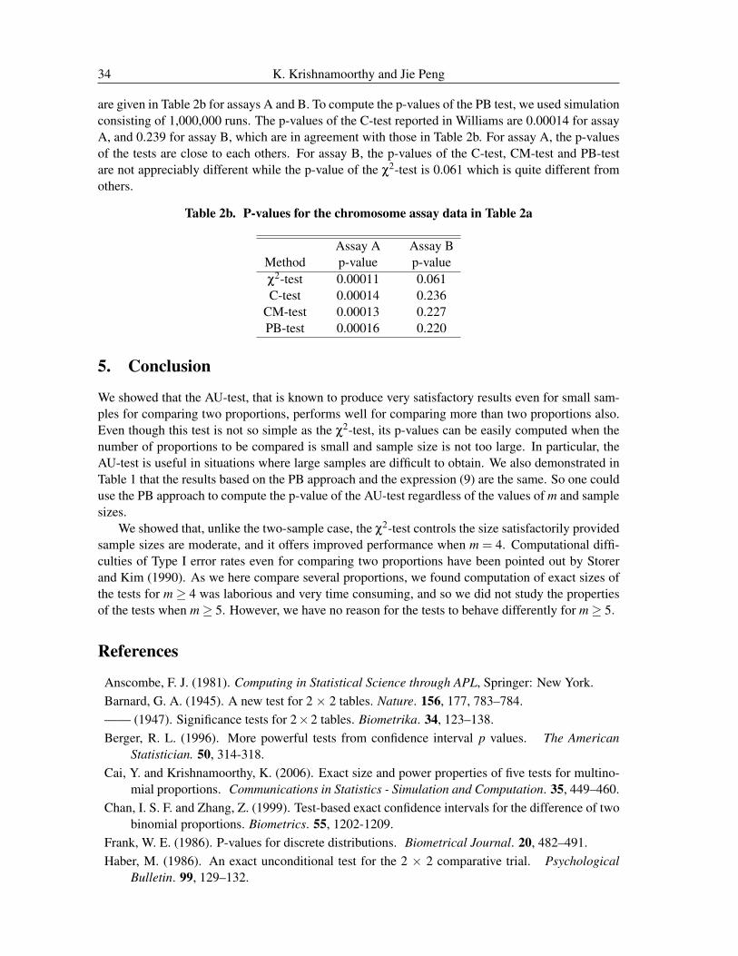
34 K. Krishnamoorthy and Jie Peng
are given in Table 2b for assays A and B. To compute the p-values of the PB test, we used simulationconsisting of 1,000,000 runs. The p-values of the C-test reported in Williams are 0.00014 for assayA, and 0.239 for assay B, which are in agreement with those in Table 2b. For assay A, the p-valuesof the tests are close to each others. For assay B, the p-values of the C-test, CM-test and PB-testare not appreciably different while the p-value of the χ2-test is 0.061 which is quite different fromothers.
Table 2b. P-values for the chromosome assay data in Table 2a
Assay A Assay BMethod p-value p-valueχ2-test 0.00011 0.061C-test 0.00014 0.236
CM-test 0.00013 0.227PB-test 0.00016 0.220
5. Conclusion
We showed that the AU-test, that is known to produce very satisfactory results even for small sam-ples for comparing two proportions, performs well for comparing more than two proportions also.Even though this test is not so simple as the χ2-test, its p-values can be easily computed when thenumber of proportions to be compared is small and sample size is not too large. In particular, theAU-test is useful in situations where large samples are difficult to obtain. We also demonstrated inTable 1 that the results based on the PB approach and the expression (9) are the same. So one coulduse the PB approach to compute the p-value of the AU-test regardless of the values of m and samplesizes.
We showed that, unlike the two-sample case, the χ2-test controls the size satisfactorily providedsample sizes are moderate, and it offers improved performance when m = 4. Computational diffi-culties of Type I error rates even for comparing two proportions have been pointed out by Storerand Kim (1990). As we here compare several proportions, we found computation of exact sizes ofthe tests for m ≥ 4 was laborious and very time consuming, and so we did not study the propertiesof the tests when m≥ 5. However, we have no reason for the tests to behave differently for m≥ 5.
References
Anscombe, F. J. (1981). Computing in Statistical Science through APL, Springer: New York.Barnard, G. A. (1945). A new test for 2 × 2 tables. Nature. 156, 177, 783–784.—— (1947). Significance tests for 2×2 tables. Biometrika. 34, 123–138.Berger, R. L. (1996). More powerful tests from confidence interval p values. The American
Statistician. 50, 314-318.Cai, Y. and Krishnamoorthy, K. (2006). Exact size and power properties of five tests for multino-
mial proportions. Communications in Statistics - Simulation and Computation. 35, 449–460.Chan, I. S. F. and Zhang, Z. (1999). Test-based exact confidence intervals for the difference of two
binomial proportions. Biometrics. 55, 1202-1209.Frank, W. E. (1986). P-values for discrete distributions. Biometrical Journal. 20, 482–491.Haber, M. (1986). An exact unconditional test for the 2 × 2 comparative trial. Psychological
Bulletin. 99, 129–132.
Exact Properties of a New Test and Other Tests... 35
Krishnamoorthy, K. and Thomson, J. (2002). Hypothesis testing about proportions in two finitepopulations. The American Statistician. 56, 215–222.
—————– (2004). A more powerful test for comparing two Poisson means. Journal ofStatistical Planning and Inference. 119, 23–35.
Krishnamoorthy, K., Thomson J. and Cai Y (2004). An exact method for testing equality of severalbinomial proportions to a specified standard. Computational Statistics and Data Analysis.45, 697–707.
Kulkarni, P. M. and Shah, A. K. (1995). Testing the equality of several binomial proportions to aprespecified standard. Statistics & Probability Letters. 25, 213–219.
Lancaster, H. O. (1961). Significance tests in discrete distributions. Journal of the AmericanStatistical Association. 56, 223–234.
Martin, A. A. and Silva, M. A. (1994). Choosing the optimal unconditioned test for comparingtwo independent proportions. Computational Statistics and Data Analysis. 17, 555–574.
Martin, A. A. and Sanchez, Q. M. J. and Silva, M. A. (1998). Fisher’s mid-P-value arrangementin 2×2 comparative trials. Computational statistics and data analysis. 29, 107–113.
————– (2002). Asymptotical tests in 2 × 2 comparative trials (unconditional approach).Computational Statistics and Data Analysis. 40:339–354.
Storer, B. E. and Kim, C. (1990). Exact properties of some exact test statistics comparing twobinomial proportions. Journal of the American Statistical Association. 85, 146–155.
Scheaffer, R. L. and McClave, J. T. (1994). Probability and Statistics for Engineers. DuxburyPress: Pacific Grove, CA.
Upton, G. J. G. (1982). A Comparison of alternative tests for the 2× 2 comparative trial. Journalof the Royal Statistical Society, Ser. A. 145, 86–105.
Williams, D. A. (1988). Test for differences between several small proportions. Applied Statistics.37, 421–434.
Zar, J. H. (1999). Biostatistical Analysis. Prentice Hall: New York.