Ex-Post Costs and RIN Prices Under the Renewable Fuel Standard

Gabriel E. Lade,a,c C.-Y. Cynthia Lin,a,b and Aaron Smitha,*

Department of Agricultural and Resource Economics University of California, Davis

January 30, 2015

Abstract

We critically review the Environmental Protection Agency’s assessment of the costs and benefits of the Renewable Fuel Standard as summarized in its Regulatory Impact Analysis (RIA). We focus particularly on the EPA’s methods used to calculate costs of the policy on the US fuel market. We compare the EPA’s ex ante cost and benefit estimates to measures of ex post costs implied by the price of compliance credits under the policy. Overall, we find that the Agency’s assessment was inadequate. In spite of, or perhaps because of, the detailed and complex analysis underlying the RIA, the EPA overlooked several fundamental factors. We conclude by recommending a simplification of the analysis used in RIAs, as well as recommend the use of ‘stress tests’ in RIAs to ensure that programs like the RFS2 are designed in ways that can manage high compliance cost scenarios.

a Department of Agricultural and Resource Economics, University of California, Davis. b Department of Environmental Science and Policy, University of California, Davis. c Corresponding author: gelade@ucdavis.edu. * We gratefully acknowledge support for this research from Resources for the Future through its Regulatory Policy Initiative grant. Robert Johansson, Richard Morgenstern, Arthur Fraas, Winston Harrington, Randall Lutter, Arik Levinson, participants at the RPI authors meetings, and an anonymous referee provided invaluable comments.

1. Introduction The Renewable Fuel Standard (RFS2) seeks to expand US biofuel consumption to 36 billion gallons (bgals) per year by 2022, which would displace approximately 25% of current fuel demand. The RFS2 was created by the Energy Independence and Security Act (EISA) of 2007, which expanded the original Renewable Fuel Standard passed by Congress two years earlier. The program is administrated by the Environmental Protection Agency (EPA). In February 2010, the EPA released an extensive Regulatory Impact Analysis (RIA) studying the benefits and costs of the policy ex ante. In this paper, we critically review the Agency’s RIA. We pay particular attention to the EPA’s methods used to estimate costs of the policy on the US transportation fuel market, which constitutes the Agency’s largest share of ex ante benefits. We compare the EPA’s estimates to two useful ex post measures implied by the price of RFS2 compliance credits. First, we use the compliance credit prices to quantify the policy-induced transfers from gasoline and diesel producers to biofuel producers. These transfers reveal the incentives for industry participants to lobby for or against the policy and thereby show the potential for such lobbying to derail the policy. Second, we use the credit prices to estimate an upper bound on the increase in wholesale gasoline and diesel prices due to the policy. The second measure provides a direct estimate with which we compare the Agency’s ex ante cost estimates. Overall, we find that the Agency’s RIA overlooked three important factors, which led to an overly optimistic characterization of fuel market impacts of the RFS2. First, the Agency did not consider delays in the development of the advanced biofuel industry. Second, it did not account for delayed investments in alternative fuel vehicles and fueling infrastructure necessary to consume more than 10% ethanol-gasoline blends. Finally, the EPA did not properly characterize the uncertainty inherent in predicting future relative prices of oil and biofuels. The shortcomings of the RIA contributed to the problems currently facing the Agency in implementing the RFS2. As of January 2015, the EPA has failed to finalize the mandate requirements for 2014, and will likely not finalize the 2014 or 2015 mandates until mid-2015. In addition, the Agency has vastly scaled back requirements for cellulosic biofuel since 2010, and has proposed large cuts to the 2014 total biofuel mandate. The proposed cuts were the direct result of high compliance costs arising due to the issues highlighted above. We identify four reasons that the RIA overlooked these factors. First, the Agency relied on a set of large scale engineering and economic models to determine the costs of the policy in the long run only (post 2022). Large-scale models generate numerous statistics and require substantial effort to implement. Such detailed output creates the impression of rigor and precision, when in fact it reflects numerous modeling assumptions made about the relevant economic systems. If these assumptions are incorrect, then the results can be grossly incorrect. Second, the Agency relied on only two counterfactual reference cases and three essentially equivalent control cases to compare the costs and benefits of the policy in 2022, and omitted scenarios with low crude oil and high feedstock prices in its counterfactual cases. The most important factor driving the estimated fuel market costs of the RFS2 is the relative price of crude oil to the price of biofuel feedstocks; however, its importance is obscured in the RIA. By relying on large scale models, the Agency

2

limited its ability to study an adequate number of alternative scenarios to properly characterize the economic uncertainty inherent in predicting future fuel and agricultural market prices. Last, the Agency used average rather than marginal costs to assess fuel market impacts of the RFS2, and omitted scenarios that consider important production, consumption, or distributional capacity constraints that are inherent in energy markets. Fundamental principles of economics dictate that fuel prices are set by marginal costs. In addition, capacity constraints act in a similar manner as high marginal costs. At the time the EPA wrote the RIA, the US fuel market was incapable of consuming more than 10% ethanol-gasoline blends, a constraint known as the blend wall. By failing to account for potential high marginal production costs and the effect of capacity constraints on market outcomes, the EPA overlooked important costs of the policy. The problems highlighted above lead to an incorrect assessment of costs and benefits of the RFS2. Regulatory Impact Analyses were established with the intention of ensuring that agencies fully account for and justify the costs of regulatory or legislative initiatives. The RFS2, however, is in many ways different from historical EPA regulations. Many of the EPA’s past rules have sought to control emissions or effluents in the presence of a known control technology.1 In these scenarios, estimating the costs of a regulation as the difference in capital and fuel expenditures between scenarios with and without the regulation provides a reasonable estimate of the costs of the regulation.2,3 In contrast, the advanced biofuel industry did not exist when the Energy Independence and Security Act was passed in 2007. Moreover, few vehicles on the road were able to use fuels containing high blends of biofuel, and distribution and fueling infrastructure for high biofuel blend fuels were non-existent. As a result, meeting the RFS2 mandates relies on large advances in both scientific knowledge and engineering feats, as well as the uncoordinated investment of millions of economic agents. Because of this, evaluating multiple compliance scenarios as well as “worst case” scenarios that anticipate mid-term compliance problems is essential in properly assessing potential costs of a policy such as the RFS2. In light of our review, we believe current RIAs are not well suited to evaluating policies like the RFS2. Instead, the RFS2 RIA should have used a simpler analysis of fuel and agricultural market impacts. Simpler economic models would have allowed the Agency to conduct more uncertainty analysis. If our suggested practices are adopted in future RIAs, the process could serve an additional role as a venue to ‘stress test’ policies by studying a number of ‘worst-case’ scenarios. Stress tests can be used to study whether regulations are designed to handle a wide range of plausible future outcomes. Over a decade ago, the National Research Council recommended that the EPA move towards a model of presenting

1 For example, under the Clean Air Act Amendments, the EPA established a cap and trade program for SO2 emissions. At the time, the EPA could have achieved the required emission reductions by requiring all major emitters to install “scrubbers,” or technologies that remove SO2 from power plant emissions. Because firms were able to trade compliance credits, using the costs of installing scrubbers in all facilities as an estimate of the total costs of the cap and trade program would have represented a “maximum potential cost” of the regulation to the industry. Ex post, costs were much lower than this maximum potential cost, as the economic incentives created by the cap and trade program resulted in the industry meeting the requirements of the program at much lower costs. 2 As brought up by a number of authors including Ryan (2012), even with more traditional types of regulations, the RIA methods do not consider other costs of the policies such their potential to increase barriers to entry in industries and increase market concentration. 3 In addition, doing so may overstate costs if the regulation provides the regulated industry flexibility in meeting their compliance obligations (Harrington et al., 2000).

3

multiple scenarios in RIAs and highlighting uncertainty inherent in studying the health benefits of rules (NRC, 2002). We call for similar measures in treating economic uncertainty in future RIAs. 2. Background

Passed in December 2007, the Energy Independence and Security Act (EISA) laid a path to reduce greenhouse gas emissions from the transportation sector, increase farm income, and promote energy security. To achieve these goals, EISA sought to decrease US oil imports, increase domestic energy production, and increase the efficiency of the US vehicle fleet. EISA created and expanded several policies, including increasing Corporate Average Fuel Economy standards for new vehicles, creating requirements for federal alternative fueled vehicle acquisitions, establishing more stringent standards for large electric durables, and increasing mandates for biofuel consumption in the US. The expansion of the Renewable Fuel Standard was the most ambitious provision of the law. EISA increased the original Renewable Fuel Standard, established under the Energy Policy Act of 2005, from requiring just over 7 billion gallons (bgals) of biofuel consumption per year by 2012 to 36 bgals per year by 2022. In addition to expanding the overall biofuel mandate, EISA created separate mandates for four biofuel categories:

1. Cellulosic Biofuel – Biofuel produced from the non-edible portion of plants, woods or grasses;

2. Biodiesel – Biofuel most commonly produced from oilseed such as soybean or canola oil; 3. Advanced Biofuel – Biofuel with lifecycle emissions at least 50% below a baseline value set

under EISA, including cellulosic biofuel and biodiesel but excluding ethanol produced from corn starch;

4. Renewable Biofuel – All approved biofuel, including biofuel derived from corn starch. As illustrated in Figure 1, the mandate has a nested structure such that cellulosic biofuel and biodiesel count towards their own respective mandates, the advanced biofuel mandate, and the renewable fuel mandate. Advanced biofuels such as sugarcane ethanol that do not qualify as either cellulosic biofuel or biodiesel count towards both the advanced and overall renewable biofuel mandates. Ethanol derived from corn starch, the largest feedstock for biofuel in the US, can be used only to meet the total biofuel mandate. Thus, the amount of corn ethanol that can be used towards compliance each year is capped by the volume of overall renewable biofuel mandated less the total advanced biofuel mandate. Figure 2 graphs the volumetric requirements for each category specified by EISA.4 Mandates in early years were designed so that they could be met predominantly with corn ethanol. After 2015, however, the amount of corn ethanol that can count towards compliance is capped at 15 bgals. The remaining mandate must be met with advanced biofuel, particularly cellulosic biofuel.

4 Certain biofuels generate more than one RIN per gallon. The relationship between biofuel production and RIN generation is determined by the ‘equivalence value’ (EV) of the biofuel set by the EPA. For example, every gallon of biodiesel and non-ester renewable diesel generates 1.5 RINs, so the EVs for the fuels are 1.5. To avoid confusion, in all figures and discussions in this paper we refer to the number of RINs required for compliance for each mandate category. The volumetric production requirement differs slightly depending on the composition of fuel derived from fuels with higher EV values. This allows us to compare RIN prices across all RIN types directly.

4

Each year the EPA is required to release a Proposed and Final Rule specifying the mandates for the next compliance year. While EISA specified mandates for each category through 2022, the Agency has a certain degree of flexibility in setting each the mandates each year. In particular, the Agency is able to waive or reduce the mandate if it determines that there is either inadequate domestic supply of biofuel or if the mandate would cause harm to the economy or environment (Coppess, 2013). Obligated parties are defined as refiners, blenders and importers of gasoline and diesel. The EPA implements the policy each year by specifying a share standard, or blend requirement, for each of the four biofuel categories. The Agency determines the blend requirement each year by dividing the volumes specified in its Final Rule by projected gasoline and diesel consumption.5 To determine their compliance obligation, obligated parties multiply each category’s blend requirement by the volume of gasoline or diesel they sell for final consumption. This amount is known as the renewable volume obligation (RVO). To create flexibility for obligated parties to comply with the policy, the EPA established a compliance credit trading scheme. Under the RFS2, every gallon of approved biofuel produced or imported in the US generates a credit known as a Renewable Identification Number (RIN). Once the biofuel is sold or blended for final consumption, the RIN is ‘detached’ from the biofuel and can be sold to obligated parties. To maintain compliance with the standard, obligated parties must turn in, or retire, an amount of RINs equal to their RVO. Thus, obligated parties comply with the RFS2 either by producing and blending biofuels themselves, generating their own RINs, or by purchasing RINs from other parties. The RFS2 allows firms to over- or under-comply with the mandates from year to year, but places restrictions on firms’ ability to do so. Specifically, firms can only use RINs from the previous compliance year to meet up to 20% of their RVOs each year. Similarly, the Agency allows firms to “borrow” from future compliance obligations by carrying a RVO deficit from one year to the next; however, firms are only allowed to do so for one year. To date, obligated parties have largely over-complied with their mandate requirements. Lade, Lin and Smith (2015) provide evidence that the 20% banking restriction was likely binding from 2008-2011. The aggregate volume of banked RINs was approximately 2.6 bgals in 2013, representing just over 15% of the 2013 total renewable fuel requirement. In 2014, banked RINs will likely be just under 1.9 bgals (Paulson, 2014). EISA requires the EPA to release a Final Rule for each compliance year by November of the prior year. The EPA is also required to release a Proposed Rule well in advance of the Final Rule to allow for public and stakeholder comment. Since 2013, the EPA has failed to comply with this requirement. The Agency did not release the 2013 Proposed Rule until the end of January 2013, and the Final Rule was not released until August of that year. The EPA released the Proposed Rule for 2014 in November 2013, however, as of January 2015 the Final Rule has yet to be published.

5 The standard for category j is determined by:

𝑆𝑆𝑆𝑆𝐷𝐷𝑗𝑗,𝑡𝑡 =𝑅𝑅𝑅𝑅𝑉𝑉𝑗𝑗,𝑡𝑡 × 𝑀𝑀𝑗𝑗

𝐺𝐺𝑡𝑡𝑝𝑝 + 𝐷𝐷𝑡𝑡

𝑝𝑝 − 𝐸𝐸𝑡𝑡

where 𝑆𝑆𝑆𝑆𝐷𝐷𝑗𝑗,𝑡𝑡 is the share standard for category j in year t, 𝑅𝑅𝑅𝑅𝑉𝑉𝑗𝑗,𝑡𝑡 is the renewable fuel volume of category j fuel specified by EISA, 𝑀𝑀𝑗𝑗 is the renewable fuel multiplier for category j biofuels, 𝐺𝐺𝑡𝑡

𝑝𝑝 and 𝐷𝐷𝑡𝑡𝑝𝑝 are projected gasoline and

diesel production from qualifying sources, and 𝐸𝐸𝑡𝑡 are exempted sources such as fuel produced by small refiners.

5

Figure 3 compares the volumes specified in the EPA’s Final Rules with the volumes specified in EISA.6 Until 2014, the EPA mandates kept pace with the total biofuel mandate from EISA. Due to the delayed commercialization of cellulosic biofuel production, the Agency expanded the advanced biofuel mandate to account for the lack of cellulosic ethanol production. It also shifted biodiesel compliance obligations from 2009 to 2010 due to regulatory delays. In its 2014 Proposed Rule, however, the EPA called for drastic reductions in the overall renewable biofuel mandate. As it currently stands, the proposed 2014 overall mandate is more than 1 bgals less than the 2013 overall standard, and over 3 bgals lower than the requirements under EISA. 2.1. Challenges to Meeting the EISA Targets The RFS2 relies on the expansion of biofuel production capacity, distribution systems, fueling infrastructure, and (in the absence of drop-in biofuels) investments in vehicle technologies that can consume high-blend ethanol fuels.7 The two largest challenges facing the program are the blend wall and the lack of development of cellulosic fuel production at commercial levels. The blend wall refers to the notion that consuming greater than 10% ethanol content at a national level is costly. Oil refiners and blenders do not choose the optimal percentage of ethanol along a continuum. Air quality regulations and the need to coordinate across refiners due to shared pipeline infrastructure mean that ethanol is mostly blended at two levels in the United States: (i) 10% (referred to as E10); and (ii) and 85% (referred to as E85).8 Until 2013, the dominant means of compliance with the RFS2 was to expand E10 blends throughout the US, to the point where very little fuel currently sold in the US is E0 (fuels containing no ethanol). Given the current state of fueling and distributional infrastructure in the US, the most viable options to overcome the blend wall are to expand E85 and biodiesel consumption. The Renewable Fuel Association, the main ethanol industry trade group, estimates that only around 3,250 stations sell E85, representing less than 2% of US gasoline stations.9 In addition, only about 16 million of over 250 million registered passenger vehicles are flex-fuel vehicles (FFVs), or vehicles that are able to use E85. As a result, relatively little E85 is sold in the US today. 10 Increasing E85 consumption could be achieved by

6 The 2014 standards are from the EPA Proposed Rule for 2014. 7 Drop-in biofuels are fuels derived from biomass but have the same hydrocarbon properties of gasoline, diesel or jet fuel. These fuels can be blended directly with fossil fuels with no changes to the properties of the fuel. If developed, engine and distribution compatibility problems would no longer be an issue. While both private and public sectors have attempted to develop viable drop-in fuels, the development of economical and scalable production technologies remains largely elusive. 8 In addition to E10 and E85, in 2011 the EPA granted a partial waiver of Clean Air Act Amendment requirements that allow fuel retailers to sell E15 (15% ethanol), but only to vehicles that are model year 2001 and newer. Due to many factors, little to no E15 has been sold to date in the US and the blend seems unlikely to be expanded. As a result, we do not consider compliance through expanded E15 consumption further here, though future circumstances may increase its use. 9 See http://www.ethanolrfa.org/pages/e-85. 10 The problem is further complicated by the fact that many of the FFVs in the US are located in states with little E85 fueling capacity (Babcock and Poliout, 2013). This due to the fact that FFV adoption to date has largely been driven by incentives set by CAFE standards that inflated the accounting of fuel economy for FFVs rather than by demand for the technology (Sallee and Anderson, 2011).

6

discounting E85 below energy parity costs; however, doing so would require high RIN prices and would be a costly compliance option in the short to medium term (Babcock and Poliout, 2014).11 An alternative to expanding E85 is to increase biodiesel or renewable diesel blending. Both fuels are chemically more similar to diesel fuel than ethanol is to gasoline, so they face fewer blending constraints than ethanol. As of May 2014, the biodiesel industry consisted of just over 100 plants with nameplate production capacity around 2 bgals per year.12 Biodiesel is costly to produce, however, which limits the degree to which the industry can comply with the RFS2 overall mandates by expanding biodiesel production. The second largest challenge to the RFS2 is the lack of development of a cellulosic biofuel industry. As illustrated in Figure 2, EISA envisioned the development of a large advanced fuel industry able to produce large volumes of biofuel from cellulosic feedstocks, especially post 2015. By 2022, EISA mandates for cellulosic biofuel are set at 16 bgals, representing over half of the total biofuel mandate. To date, however, only very small scale commercial cellulosic biofuel production has come online.13 2.2. Relevant Literature Early work by Harry de Gorter and David Just establishes the basic economics of the RFS2 (de Gorter and Just, 2008; de Gorter and Just, 2009). More recent work studies general equilibrium effects of the policy and compares welfare outcomes under the RFS2 with other policies to reduce GHG emissions (Chen et al. 2015; Holland et al. 2015; Rajagopal et al., 2011; Lapan and Moschini, 2012), explores unintended consequences of the policy such as in reducing petroleum costs per vehicle mile traveled (Khanna et al., 2008), and studies efficiency gains from incorporating cost containment provisions into the policy in the face of high marginal compliance costs (Lade and Lin, 2015). Lade, Lin and Smith (2015) provide the first study of RIN market dynamics. The paper develops a dynamic model of an industry complying with the RFS2 over time in order to understand RIN prices. In addition, the authors estimate historical RIN price drivers, test for market efficiency, and analyze the effects of three policy shocks that reduced expected 2014 mandate levels. An important insight from the literature is that the RFS2 is equivalent to a policy that imposes a revenue neutral subsidy for biofuel production funded by a tax on gasoline and diesel sales. The result has parallels with the symmetry between cap-and-trade and tax policies. Lade, Lin and Smith (2015) show that the implicit tax on fossil fuels under the RFS2 equals the RIN price multiplied by the blending requirement for each year,14 and we use the result to generate an ex post measure of costs of the RFS2 in Sections 5.3 and 5.4.

11 A gallon of ethanol contains approximately 70% of the energy as a gallon of gasoline. As a result, FFV drivers get lower mileage for each tank of E85 versus E10. Thus, to account for the loss in energy efficiency, E85 must be priced around 30% lower than gasoline. 12 See http://www.eia.gov/biofuels/biodiesel/production/. 13 In May 2014, the Oil Price Information Service (OPIS) released a report on the state of the cellulosic fuel industry. The report detailed six cellulosic biofuel plants that are expected to produce fuel in 2014; however, little production has been realized due to both technical and financial difficulties ongoing with all plants. 14 Specifically, the implicit tax imposed by the RFS2 on gasoline and diesel is equal to 𝛼𝛼𝑗𝑗 × 𝑝𝑝𝑗𝑗𝑅𝑅𝐼𝐼𝐼𝐼, where 𝛼𝛼𝑗𝑗 is equal to the blending requirement for mandate j and 𝑝𝑝𝑗𝑗𝑅𝑅𝐼𝐼𝐼𝐼 is equal to the RIN price for mandate j.

7

Two additional literatures have emerged studying effects of the RFS2 that are germane to the current study. The first literature studies greenhouse gas (GHG) reductions from the policy, and the second studies the effect of the policy on world grain prices. We briefly survey important articles in both literatures to provide a context and background for each, though we do not provide a comprehensive study of either topic. While most life-cycle assessments of biofuels find moderate GHG reductions from corn-based biofuel, many stakeholders and academics have raised concerns about the effect of the RFS2 on total land use. If total planted acreage expands due to the RFS2, the policy would lead to large GHG releases that would otherwise be sequestered in soils.15 Searchinger et al. (2008) find using the GREET model16 that under certain assumptions about the responsiveness of planted acreage to agricultural price increases, the RFS2 could lead to substantial increases in planted land, resulting in large releases of GHG emissions. The issue remains highly contentious and no consensus has been reached in the literature.17 Many commentators and academics have pointed to increased demand for corn, soybeans, and other agricultural feedstocks for biofuel production as a key contributor to the higher prices and volatility observed in grain markets recently. Since 2005, world grain markets have experienced substantial and sustained price spikes that have had important implications for the food security of the world’s poor and political stability of many developing countries (Wright, 2014). Several studies have estimated the effect of the RFS2 on grain prices. Hausman, Auffhammer, and Berck (2012) find that 27% of the increase in the price of corn from 2006 to 2007 can be attributed to increased demand for biofuels. Carter, Rausser and Smith (2013) estimate that average corn prices were over 30% higher from 2006-2012 than they would have been in the absence of the RFS2. Roberts and Schlenker (2013) aggregate corn, rice, wheat and soybeans into a single index and estimate that this price index would be 20% lower without US ethanol production. In light of these findings, there is justified concern that much of the price increases and volatility observed in grain markets since 2005 is attributable to increased demand for fuel production in the developed world. While RIA’s typically only consider domestic market disturbances, these findings imply significant negative effects on the welfare of the world’s urban poor and corresponding positive effects on the world’s rural poor. 3. Framework for Evaluating Fuel Costs and Welfare of the RFS2 In this section, we present a model of a gasoline industry faced with a biofuel mandate to illustrate the market effects of the RFS2. The model establishes a framework with which we evaluate the EPA’s cost

15 Life-cycle assessments (LCA) attempt to measure the total environmental impacts of a production process from “cradle to grave.” The LCA community attempts to measure the GHG emissions from extraction, production, distribution, and consumption of alternative fuels to compare the environmental impacts from various feedstocks. 16 The GREET model is maintained by Argonne National Laboratory and is a commonly used model to estimate total emission impacts of alternative fuels. 17 See Wang et al. (2012) for a more recent study of lifecycle GHG impacts of ethanol from corn, sugarcane and cellulosic using the GREET model that incorporates emissions from land use change. Witcover et al. (2013) summarize much of the literature on indirect land use change to date and discuss policy options to address the issue.

8

and benefit estimates, and motivates our measures of ex post costs. The model is necessarily simple. For an example of a more complete economic analysis of the welfare effects of the RFS2, see Chen et al. (2014). Our model shows the deadweight loss in the fuel market resulting from the policy. A complete cost-benefit analysis would weigh this deadweight loss against the non-fuel market benefits of the policy. These potential benefits include reduced greenhouse gas emissions, increased energy security, and decreased (or increased) health effects from local pollutants. If the value of the benefits exceeds the deadweight loss in the fuel market, then the welfare gains from the policy are positive. Consider a gasoline and ethanol market in which in the absence of any government policy little biofuel is blended into fuel sold to consumers.18,19 Figures 4(a)-4(c) graph the initial market equilibrium in the ethanol, gasoline, and final blended gasoline markets, respectively. The blended gasoline supply curve, the upward sloping curve in Figure 4(c), is equal to the horizontal sum of the ethanol and gasoline supply curves in Figures 4(a) and 4(b), respectively. Market equilibrium occurs where fuel demand equals the supply of blended gasoline, and the equilibrium volumes of ethanol and gasoline are found by observing the supply of each fuel at the market clearing price. Figures 4(d)-4(f) graph the market equilibrium under a RFS2. The dashed lines represent the supply curves net of the tax or subsidy effect of the RFS2. As discussed in the previous section, a biofuel mandate provides an implicit subsidy for the ethanol, making every gallon cheaper because it generates a RIN that can be sold to producers of gasoline. At the same time, the policy implicitly taxes gasoline as gasoline producers must purchase 𝛼𝛼 RINs for every gallon of gasoline produced, where 𝛼𝛼 is the blend requirement. Thus, the policy induces a transfer between the ethanol and fossil fuel industries, equal to the box defined by A+B in Figure 4(d) and box D+E+F in Figure 4(e). This amount is equal to the value of the gasoline industry’s renewable volume obligation. By definition, a binding ethanol mandate is costly to fuel markets because it requires the market to blend more ethanol than it would in the absence of the policy. This is illustrated by the upward shift in the blended gasoline supply curve in Figure 4(f).20 The resulting equilibrium involves a higher blended fuel price and lower consumption, creating deadweight loss in the market. The deadweight loss represents the economic cost of the policy, and is equal to the decrease in producer surplus to conventional fuel producers (F+G) plus the decrease in consumer surplus to fuel consumers (H+I+J) minus the increase in producer surplus for ethanol producers (A+C). In terms of the labeled areas in Figure 4, the deadweight loss can be expressed as:

𝐷𝐷𝐷𝐷𝐷𝐷 = −(𝐴𝐴 + 𝐶𝐶) + (𝑅𝑅 + 𝐺𝐺) + (𝐻𝐻 + 𝐼𝐼 + 𝐽𝐽)

18 We implicitly assume that biofuel and blended fuel are perfect substitutes in production and consumption. 19 The analysis here can equivalently be applied to the diesel and biodiesel market. 20 A binding renewable fuel mandate may decrease blended fuel prices if the elasticity of renewable fuel is large enough such that the decrease in the supply of gasoline is more than offset by the increase in the supply of ethanol with a RFS2 (de Gorter and Just, 2009; Fischer, 2010). While this situation is theoretically plausible, simulation based studies of the RFS2 have consistently found the policy increases fuel prices using plausible supply elasticity estimates (see e.g., Lade and Lin, 2015; Chen et al., 2014). Nonetheless, the policy would remain costly to fuel markets in this scenario as well, as an overall decrease in fuel prices due to the policy would be associated with its own DWL.

9

The cost-benefit framework presented here excludes spillover effects into other markets. Potential spillovers include distortions to agricultural markets and other fuel markets. For example, an increase in demand for corn from ethanol producers causes farmers to grow corn rather than other crops and it causes corn users to substitute to other commodities. Similarly, a reduction in the quantity of gasoline demanded spills over into other petroleum products such as heating oil and diesel. Spillovers can be incorporated into Figure 4, however, by conceptualizing the supply and demand curves as general equilibrium curves, i.e., curves that do not hold constant the prices in other markets (see Harberger (1964) and Thurman (1991)). Next, we evaluate the EPA’s analysis in light of this modeling framework. 4. The EPA’s Regulatory Impact Analysis

The EPA released its Regulatory Impact Analysis (RIA) in early 2010. The RIA quantifies the costs and benefits of increased production, distribution and consumption of renewable fuels. To do this, the EPA uses two primary reference cases as estimates of how the industry would evolve in the absence of the RFS2:

i. Projections made in the 2007 Annual Energy Outlook (AEO) of gasoline, diesel, and renewable fuel consumption by the Energy Information Administration;

ii. Projections using the renewable fuel volumes mandated under the RFS1. The reference cases are compared to three primary control cases, or outcomes with the RFS2:

i. The renewable fuel schedule specified in EISA; ii. A “low-ethanol” control case assuming the cellulosic biofuel mandate is predominantly met

with cellulosic diesel; iii. A “high-ethanol” control case assuming the cellulosic biofuel mandate is met in full with

cellulosic ethanol. The EPA calculated its cost and benefits of the RFS2 by comparing outcomes under the reference cases to outcomes under the control cases. Most modeling efforts focused on predicting effects of the policy in 2022. In doing so, the EPA assumed all necessary investments in vehicle, production, distribution, and fueling infrastructure were made as needed to meet the requirements of the program. Table 1 summarizes the long run costs and benefits estimated by the RIA. Overall, the EPA finds very large net benefits from the RFS2 in 2022 with estimates ranging from $12.8-$25.97 billion a year. The estimates equal the sum of estimated fuel market benefits, non-market benefits to energy security, health, and GHG emissions attributed to the policy in that year. As can be seen, the benefits to fuel markets attributed to the RFS2 constitute the vast majority of the overall benefits. The fuel market benefits in Table 1 immediately bring to bear an important conceptual flaw of the RIA. Namely, estimating that the RFS2 dramatically reduces fuel market prices is inconsistent with the notion that a binding regulation can only increase total costs in a market. Thus, the EPA’s estimates imply the RFS2 is non-binding on fuel markets in the long run. In the remainder of this section, we describe in more detail the calculations underlying the estimates in Table 1.

10

4.1. Fuel Market Impacts To calculate fuel market impacts in 2022, the EPA used energy demand projections from the 2007 AEO and compared fuel expenditures across the reference and RFS2 control cases holding constant demand for vehicle miles traveled. Thus, the EPA assumed energy demand was perfectly inelastic and would be unaffected by fuel composition or price differences across the various reference and control cases. The Agency disaggregated its fuel market cost calculations by PADD using a refinery model frequently used by the fossil fuel industry to estimate costs of producing gasoline and diesel from various feedstocks.21 To calculate gasoline and diesel prices the Agency used projection of crude oil prices developed for the 2007 AEO. The projections assumed average crude oil prices would be approximately $55/bbl (2007 dollars) in 2022. The EPA used the FASOM model, a dynamic nonlinear programming model of the US agricultural sector, to estimate biofuel input and production costs. Using historical spreads between biofuel, gasoline, and diesel disaggregated by season and PADD and assuming distribution costs for transporting and blending biofuels, the Agency ran their refiner optimization model under each control and RFS2 reference case. Given the price and input-output requirements under each scenario, the model produced detailed tables of refinery inputs and outputs by PADD and season. Using the volumes of the various refining inputs and outputs produced by the refining model runs, the Agency compared fuel expenditures under the references versus control cases. While the Agency used 2007 AEO prices and quantities as inputs to their refining model, they used oil price projections from the 2009 AEO central reference case to calculate wholesale gasoline and retail prices. Figure 5 graphs the change in the EIA’s oil project projections from 2007 to 2009. As can be seen, the central reference case is substantially higher in the 2009 AEO. Using 2009 AEO year-on-year oil price projections and FASOM feedstock projections, the Agency also calculated year-on-year average fuel expenditures impacts, recreated in Table 2. As can be seen, given their price projections, the Agency estimated that fuel expenditures due to the RFS2 would decrease on average in both the gasoline and diesel markets by 2016. Overall, the EPA estimated that gasoline prices will be $0.024/gal lower and diesel prices will be $0.121/gal lower in 2022 under the primary RFS2 control case than the 2007 AEO case. The EPA also calculated net capital cost expenditures under the control and RFS2 reference cases. The estimates include costs of building the necessary biofuel production facilities, building a distribution network for biofuels, the cost of increased FFVs and FFV fueling infrastructure, and savings from decreases in refinery capacity investments. Overall, the EPA estimated a range of $68.5 to $110 billion in capital investments required from 2010-2022 to meet the RFS2 relative to the 2007 AEO, with an estimate of $90.5 billion for the primary control case. Capital investment cost estimates, however, are excluded from the total cost of the policy because the annual cost of capital should be incorporated in to biofuel prices. The Agency also included estimates of energy security benefits of the RFS2. The Agency estimated energy security benefits in two components: (i) avoided macroeconomic dislocation costs associated

21 PADD refers to Petroleum Administration for Defense Districts and are common unit for fossil fuel statistics used by the US government.

11

with oil and renewable fuel price volatility; and (ii) monopsony benefits associated with reduced oil imports. The EPA decomposed the former into ‘aggregate output losses’ or losses in US output due to increased oil prices, and ‘allocative losses’ or losses due to temporary underutilization of capital and labor in the US due to an oil price shock. The Agency assumed the introduction of renewable fuels both reduces the supply elasticity of motor fuels and diversifies the US economy’s fuel portfolio towards volatile sources. Using an assumed elasticity of GDP with respect to oil price shocks, the EPA estimates a dollar per barrel estimate of reduced macroeconomic dislocation costs from the RFS2 control case versus the AEO 2007 reference case. Overall, the EPA estimated energy security benefits in 2022 from the RFS2 at $2.6 billion. 4.2. GHG emission and air quality impacts The EPA has extensive experience estimating air quality and greenhouse gas impacts of policies. Given the specified volumes of various biofuels fuels in the control and references cases, the EPA evaluated the carbon intensity of each fuel production pathway to determine the GHG savings from the RFS2 rule. It similarly studied changes in air pollutants from increased production and combustion of biofuels under the RFS2 reference cases to determine non-GHG emission costs of the policy. To estimate GHG savings, the EPA specified the anticipated feedstocks used for advanced biofuel production as well as the anticipated production technologies that would be used to produce each fuel in 2022 (Table 2.7-1 in the RIA). The GHG savings calculations included changes in carbon dioxide, nitrous oxide, and methane emissions between the control and reference cases.22 The Agency also included emissions due to modest changes in land use for soybean, corn, and sugarcane production. The EPA estimated that the RFS2 would reduce GHG emissions by 130 million metric tons (MMt) per year.23 Based on the estimated reductions, the EPA calculated the net present value (NPV) of the stream of benefits over a 30 year horizon with a 3-5% discount rate for alternative estimates of the social cost of carbon. Overall, the EPA estimated between $0.6 and $12.2 billion in benefits due to the decrease in GHG emissions. The estimate varies based on the alternative assumptions about the social cost of carbon and the discount rate. The EPA used a similar method to calculate non-GHG emission impacts of the RFS2. The estimates included emission impacts from the production, distribution and combustion of fuels in the various fuel compositions. The estimates are complicated by the fact that calculating the costs and benefits of criteria pollutants requires knowing the composition of the various pollutants across space and over time. Overall, the EPA estimated a slight increase in the population-weighted annual ozone and PM2.5, and a slight decrease in other air toxics due to the RFS2. To the extent it could, the EPA attempted to monetize the costs of increased ozone and mortality due to increases in total criteria pollutants.

22 Changes in methane and nitrous oxide emissions are primarily due to differences in the composition of tailpipe emissions between low blend ethanol fuel (E10) and higher blend ethanol fuel (E85). 23 To put the number in perspective, the EPA’s greenhouse gas inventory in 2012 estimated that total US CO2 were approximately 6,526 MMt, with the transportation sector contributing over 1,800 MMt. Thus, the estimated GHG savings in 2022 represents approximately a 7% decrease in GHG emission from the transportation sector due to the RFS2.

12

Overall, the EPA estimated a cost of between $0.63 and $2.2 billion due to increased criteria pollutants from the policy relative to the baseline scenarios.24 4.3. Agricultural Market Impacts The RIA used several large-scale economic and engineering models to estimate the impact of expanded biofuel feedstock production to meet the demands of the RFS2 in 2022 on agricultural markets. These estimates, however, were excluded from the computation of the bottom line impact estimate. The EPA estimated the impacts on both traditional crops and provided detailed estimates of production and distribution costs for advanced biofuels using different feedstocks including wood pulp, switchgrass, and corn stover. The impacts were estimated for both US and international markets, focusing on the effects of the policy on Brazilian sugarcane production. Overall, the EPA estimated an increase of $3.6 billion per year in food expenditure in the US due to the policy, representing an increase of around $10/capita. In addition, the Agency estimated a decrease of around $500 million per year in the value of corn and soybean exports, and an increase in farm income of around $13 billion per year. The results of modest price impacts are driven mainly by assumptions that corn and soybean prices would rise only 8.2% and 10.3% relative to the reference cases. While the EPA discusses the effect of the policy on international commodity markets, it does not include the cost of increased staple food prices on the world’s urban poor in its estimates. 4.4. Evaluation of Estimated Impacts As discussed in Section 3, a complete assessment of fuel market costs would take into consideration price changes due to the policy, the associated deadweight loss to consumers, and the corresponding loss in producer surplus to gasoline producers and the gain in producer surplus to biofuel producers. If the Agency wished only to compare expenditures under the various scenarios, a correct estimate of the change in fuel costs due to the RFS2 would equal the area H+I in Figure 4. While this measure would not be an estimate of the welfare effects of the policy, we agree that comparing expenditures across scenarios is a useful measure of program costs and avoids many necessary assumptions to calculate deadweight losses.25 The Agency’s estimates of fuel expenditures changes, however, were incorrect. Its estimates aggregated capital costs required to produce, distribute and consume biofuel, and estimated changes in expenditures for alternative fuel compositions. This approach produces an estimate of the average cost of supplying fuels; however, economic theory states that prices are set by marginal costs. When the marginal biofuel used to meet the RFS2 mandates is expensive, comparing fuel expenditures using average costs significantly understates the increase in fuel costs to consumers.

24 The estimates represent a lower bound as they do not consider a number of other direct and indirect effects of increased criteria pollutants (a full list of non-monetized effects are listed in Table 5.4-2 in the RIA). Other environmental impacts that were considered by the RIA included the effect of the policy on factors such as visibility, forest health, nitrogen and phosphorous loadings in the Mississippi River, among many others. 25 In addition, given that the RFS2 likely has a very small effect on retail gasoline prices (Knittel and Smith (2014)), the loss in producer surplus to gasoline producers may be quite small and, in particular, smaller than the gain to ethanol producers. Thus, it is likely that A+C>F+G. It follows that a properly estimated increase in fuel costs may overestimate the full deadweight loss of the policy.

13

In addition, despite acknowledging the vast uncertainty in projecting feedstock and oil prices in 2022, the EPA limited itself to the central oil price projections from the 2009 AEO, ignoring the high and low projections from the report (Figure 5). At the time of the writing of the RIA in 2009, world oil markets were coming off of a historical volatile period with WTI prices trading near $140/bbl in the summer of 2008 and bottoming out near $40/bbl in January 2009, demonstrating the unpredictable nature of oil markets. Despite this, the EPA failed to account for this by considering only one price trajectory. 5. Using RIN Prices as Ex Post Cost Estimates In this section, we compare costs of the RFS2 so far to EPA predictions in the RIA. Economic theory suggests that when firms are able to trade compliance credits and markets are robust, an efficient equilibrium will be reached in which marginal compliance costs are equalized across regulated parties (Montgomery, 1972).26 Because firms are allowed to bank and borrow RINs over time, both current and expected future marginal compliance costs affect the demand for RINs (Rubin, 1996; Schennach, 2000; Lade, Lin and Smith, 2015). We take advantage of this feature of credit prices to conceptualize two measures of ex post costs of the RFS2 on the US fuel industry. Specifically, we estimate the value of the transfer from conventional to biofuel producers, and compute an upper bound on the increase in fuel costs.27 Since the program’s inception, a large over-the-counter market for RINs has emerged. The Oil Price Information Service (OPIS) has surveyed obligated parties and RIN traders since 2008 and records daily high, low and average RIN prices. Conversations with regulated parties and active participants in RIN markets confirm OPIS price quotes are used as a reference when determining sale prices. We collected the entire history of conventional ethanol (D6) RINs, advanced biofuel (D5) RINs, and biodiesel (D4) RINs reported by OPIS.28,29 Given that the market for cellulosic biofuel has been essentially nonexistent to date, we do not consider costs of the cellulosic fuel mandate under the RFS2 in this paper. Before moving forward, we must establish what RIN prices reflect. In a static economic model of a competitive industry complying with a RFS, Lade and Lin (2015) show that RIN prices equal the weighted difference between the cost of the marginal (i.e., most expensive) renewable fuel used to meet each mandate and the marginal cost of the cheaper fossil fuel it displaces.30 Because obligated parties are

26 We refer to “robust” credit markets in the sense that there are no transactions costs to trading (Stavins, 1995), no uncertainty regarding the availability of trading partners (Montero, 1997), and no firm is able to exercise market power in the compliance credit market (Hahn, 1984). 27 For an analysis of the effects of the Renewable Fuel Standard on fixed and capital costs, see Yi, Lin and Thome (2015), who develop and estimate a dynamic structural econometric model to analyze the effects of the RFS on the entire cost structure of the ethanol industry, including entry costs, investment costs and exit scrap values. 28 Conventional (D6) RINs count only towards a firm’s overall RVO. Advanced (D5) RINs count both towards a firm’s advanced and total RVO. Biodiesel (D4) RINs count towards the total, advanced, and total RVO. 29 Conventional RINs have been reported by OPIS since April 2008. Biodiesel RINs have been reported since June, 2009, and advanced RINs have been reported since December 2010. 30 Specifically, Lade and Lin (2015) show in a model of a perfectly competitive industry with one fossil fuel 𝑞𝑞𝑐𝑐 and one renewable fuel 𝑞𝑞𝑟𝑟 that RIN prices must satisfy:

𝑝𝑝𝑅𝑅𝐼𝐼𝐼𝐼 =1

1 + 𝛼𝛼 [𝑆𝑆𝑟𝑟(𝑞𝑞𝑟𝑟∗) − 𝑆𝑆𝑐𝑐(𝑞𝑞𝑐𝑐∗)]

14

able to bank RINs, Lade, Lin and Smith (2015) show that prices reflect both current and expected future marginal compliance costs. In particular, they show that RIN prices are a function of: (i) expected future commodity prices and capital costs; and (ii) the expected future stringency of the policy. The finding has important implications for comparing our cost estimates with those produced in the RFS2 RIA. First, the RIA used average costs as the basis for evaluating fuel market impacts; however, the relevant cost depends on the marginal fuel used to meet the RFS2 requirements. Thus, if scenarios arise where average costs of biofuel are low, but the marginal fuel used to meet the RFS2 is high, the EPA’s original estimates will be biased downward. In addition, it may be the case that current marginal costs are low, but expected future marginal costs are high. This will put upward pressure on RIN prices in the current year, again leading to underestimates of the program’s costs. Because RIN prices reflect realized costs to the fossil fuel industry of complying with the RFS2, we use the prices to construct two useful measures. First, in section 5.3 we estimate the value of the transfer induced by the policy between the gasoline and ethanol industries. This value is given by areas D+E+F=A+B in Figure 4. While distributional effects and adjustment costs are not part of a traditional welfare analysis, an analysis that quantifies the magnitude of transfers enables a better understanding of the political environment of the policy. Deadweight loss is notoriously difficult to estimate, even ex post. The potential magnitude of transfers, however, is often easier to measure. Moreover, from a political economy perspective, distributional effects are among the most important factors influencing many policy outcomes.31 In addition, a policy that requires a large redistribution of resources from some agents to others likely entails large adjustment costs. As a result, the costs of a policy are likely positively correlated with the transfers needed to meet a policy’s requirements. Given this as well as the differences in measurability between deadweight loss and transfer estimates, we believe quantifying transfers across industry participants should be an important part of a regulatory impact analysis. As a second measure of the ex post costs of complying with the RFS2, in section 5.4 we estimate the value of the tax on gasoline and diesel wholesale markets. This value corresponds with the implicit tax (𝛼𝛼 𝑝𝑝𝑅𝑅𝐼𝐼𝐼𝐼) on gasoline illustrated in Figure 4(e). While the estimate does not measure the full retail price impact of the policy, it provides a reasonable upper bound estimate of the policy’s costs that relies few assumptions.

where 𝑝𝑝𝑅𝑅𝐼𝐼𝐼𝐼 is the market clearing RIN price, 𝛼𝛼 is the blending requirement, and 𝑆𝑆𝑗𝑗(𝑞𝑞𝑗𝑗∗) is the market supply function for fuel j evaluated at market clearing quantity 𝑞𝑞𝑗𝑗∗. 31 The study of public choice and policy making when gains from a program are concentrated has a long history in the economics literature. Tullock (1957) and Buchanan and Tullock (1962) first suggested that when gains from a policy are highly concentrated relative to its costs, ‘logrolling’ may occur in which politicians or interest groups bargain to support a law in exchange for future legislative support. The notion is similar to Coasian bargaining among policy makers and interest groups (Coase, 1960).

15

6. Results

6.1. Historical RIN prices

Figure 6 graphs historical RIN prices for conventional, advanced and biodiesel RINs.32 Until January 2013, conventional RIN prices remained quite low, trading between $0.05 and $0.10/gal. Prices increased moderately in 2009, when oil prices fell from their previous year high of nearly $140/barrel to a low of around $40/barrel while prices of agricultural commodities remained relatively stable. Overall, RIN prices from 2008-2012 reflected the low compliance costs of meeting the RFS2 when the mandates were below the blend wall. In January 2013 conventional RIN prices increased dramatically. Prices began their rise just before the release of the 2013 Proposed Rule, and continued to climb sharply following its release. In the Rule, the EPA maintained the overall biofuel mandate levels from EISA, pushing the mandate levels very close or even slightly above the blend wall. By maintaining the original volume requirements of EISA, the EPA likely changed expectations in the industry that at the time, according to some accounts, interpreted the delayed release of the rule as a signal the EPA would relax the standard (Thompson et al., 2012). Conventional RIN prices remained high through mid-2013 and continued to rise through July 2013, when they reached a peak of around $1.40/gal. In early August 2013 the EPA released its 2013 Final Rule, maintaining the volumes from the Proposed Rule. In the Rule, however, the Agency suggested it would relax the 2014 standards due to concerns about the blend wall. Immediately following the announcement, prices began as dramatic a fall as their initial rise in January. Prices fell through November 2013, when the EPA released its 2014 Proposed Rule in which it proposed the substantial cuts to the total renewable fuel mandate illustrated in Figure 3. Since July 2013, prices have traded for as low as $0.20/gal, but have gained in recent months, trading between $0.40-$0.50/gal. Biodiesel and advanced RINs have been relatively costly throughout the program’s history. Early biodiesel RINs were reported at prices near conventional ethanol RINs; however, the prices should be interpreted with caution as there was little biodiesel production at the time and many parties were concerned at the time with the sale of fraudulent biodiesel RINs. Since 2011, biodiesel RINs have generally trade above $1.00/gal, reaching nearly $2.00/gal in mid-2011 reflecting the high relative prices of producing biodiesel. Advanced RINs have traded lower than biodiesel RINs but at higher prices than conventional RINs, reflecting a binding advanced ethanol sub-mandate. After the large run-up in prices in January 2013, the prices of all RIN types converged. As discussed in Lade, Lin and Smith (2015), the convergence of the RINs across biofuel type suggests that the industry expectation was for biodiesel to be the marginal fuel pushing the industry beyond the blend wall. Since the release of the 2013 Final Rule and subsequent fall in all RIN prices, biodiesel and advanced RINs have trade at a slight premium to conventional RINs, though they generally have generally remained low.

32 The figure graphs current year RIN prices using vintage prices for the current compliance year. For example, 2010 conventional RIN prices are for 2010 vintage RINs and 2011 prices are for 2011 vintage RINs

16

6.2. A test of market rationality

Using RIN prices as an accurate measure of marginal compliance costs requires a robust market for the credits. Unlike traditional compliance credit markets under cap and trade programs, the EPA is unable to withhold RINs for sale on an auction. Instead, the Agency relies on renewable fuel producers to register their fuel pathway, generate RINs by documenting all qualifying fuel produced and sold in the US, and find trading partners to sell the credits. Given the over-the-counter nature of RIN markets and issues with fraud in the market for biodiesel RINs, several observers have questioned whether RIN markets have been efficient (Moregenson and Gebeloff, 2013).33 To test whether RIN prices have satisfied conditions for a “rational” market in the traditional economic sense of financial markets (e.g., Fama, 1965), Lade, Lin and Smith (2015) develop a test of whether historical RIN price changes were predictable. While only a necessary condition for market rationality, if RIN prices reported by OPIS were predictable using alternative forecast models, there would be strong evidence that either the prices reported by OPIS were not accurate reflections of RIN prices or that the market for RINs has been inefficient. Overall, Lade, Lin and Smith (2015) find that RIN price changes using OPIS daily RIN prices were largely unpredictable, and cannot reject the hypothesis that any of our chosen forecast models outperform the random walk model. The result is encouraging to the extent it illustrates that despite concerns regarding the validity of our data that it appears to satisfy a basic tenant of an economically rational financial market. 6.3. Value of the Renewable Volume Obligation In this section, we quantify the value of the implicit tax from the RFS2 on obligated parties, or equivalently the value of the subsidy provided by the program to the biofuel industry. Specifically, we use monthly gasoline and diesel sales data to estimate the value of the fuel industry’s RVO in each month from 2010 to present.34 Gasoline and diesel sales data are from the Energy Information Administration. The estimated monthly RVO is graphed in Figure 7(a) for July 2010 to present.35 Month to month variation in the RVO reflect cyclical changes in fuel sales in the US, while year to year increases are driven by the increase in the EPA standards. As can be seen in Figure 7(b), the RVO has increased over time, reaching nearly 2 bgals/month in 2013.

33 Several cases of fraud in the biodiesel RIN market occurred from 2009-2012 in which a few small biodiesel producers sold RINs to obligated parties for biodiesel that was never produced. During the period when the bulk of fraudulent RINs were sold, the biodiesel mandate represented a very small share of the overall mandate. For example, in 2011 and 2012 the biodiesel mandate was set at 800 million gallons and 1 billion gallons, respectively. By comparison, total biofuel consumption was set at 12.6 and 13.2 billion gallons in 2011 and 2012. 34 The true RVO includes adjustments reflecting exemptions for small refiners. We ignore the exemptions here as the EPA does not release production data for exempted sources. Our estimates therefore slightly overestimate the obligation in any period. 35 The EPA did not begin reporting RIN generation through the EMTS until July 2010. We report all estimates since this time to remain consistent with data available through the EPA reporting mechanism.

17

Figure 7(b) graphs the value of the monthly RVO since 2010, equal to the monthly RVO multiplied by each respective RIN price. Until 2013, the value of the RVO was relatively modest and never exceeding $400 mil/month. Most of the value of the RVO was driven by high advanced and biodiesel RIN prices, with conventional RINs contributing little to the cost of the program. With the run-up in RIN prices in early 2013, however, the value of the RVO for all mandates increased substantially. In July 2013, the value of the RVO peaked at just over $2 billion dollars per month. After the release of the 2013 Final Rule, however, the value of the RVO decreased sharply, falling to current levels slightly under $1 billion dollars per month. The increase in the RVO’s value in early to mid-2013 represented the necessary increase to overcome the blend wall. After the EPA implied it would likely reduce 2014 obligations, however, the value of the RVO fell dramatically, reflecting the lower expected future transfers needed to maintain compliance with a lower 2014 standard.36 The high RVO values observed since the beginning of 2013 signify large transfers from conventional to biofuel producers. The subsequent wavering of the EPA on the timing and magnitude of its RVO rules likely reflects increased lobbying pressure from the conventional fuel industry as it seeks to reduce its compliance costs. This wavering induces uncertainty about future standards that serves to undermine the statute. 6.4. Effect of the RFS2 on wholesale markets

Several authors have attempted to estimate the effect of increased biofuel blending from the RFS2 on retail fuel prices (Du and Hayes 2009, 2011, 2012; Knittel and Smith, 2014). Theoretically, the effect of the RFS2 on retail fuel prices is ambiguous. The effect depends on the supply response of biofuels to the RFS2 mandates (de Gorter and Just, 2008; Lade and Lin, 2015). Intuitively, if the increase in the supply of biofuels in response to the RFS2 is smaller than the resulting decrease in gasoline and diesel, overall fuel supply will decrease and prices will increase. For the purposes of this paper, rather than estimate the full retail price impact of the RFS2, we take advantage of RIN prices to estimate an upper bound of the policy’s costs on wholesale gasoline and diesel markets. Specifically, we use RIN prices to calculate the value of the implicit tax from each blending requirement on wholesale gasoline and diesel. So long as the marginal biofuel cost is not too high, the estimate provides a reasonable upper bound on the retail price effects of the RFS2.37 Figure 8 graphs our estimates of the implicit tax from each mandate. Until January 2013, the implicit taxes were generally less than $0.01/gal. The increase in RIN prices in 2013 increased the implicit tax from all mandates. The conventional fuel tax increased the most to around $0.12/gal. To put the amount in perspective, current federal excise taxes on gasoline and diesel are $0.184/gal and $0.24/gal, respectively, while total average state and federal gasoline tax liabilities are just under $0.50/gal (American Petroleum Institute, 2015).

36 Lade, Lin and Smith (2015) estimate that the release of the EPA’s 2013 Final Rule decreased the total value of the RVO between $7.4 and $8.4 billion dollars for the 2013 compliance year alone. The estimate represents a lower bound of the effect of the 2014 cuts, and large decreases in the 2013 RVO were also observed following two other ‘policy shocks’ revealing the level of the 2014 mandate cuts. 37 The translation of these wholesale market costs to retail fuel prices remains an open empirical question and an area for future research.

18

Table 3 compares the high, low and average values of our ex post cost estimates in each year to the EPA’s ex ante predictions of average gasoline and diesel market impacts for 2010-2014. Because the advanced biofuel mandate has predominantly been met with imported sugarcane ethanol, we compare the sum of the implicit tax from the conventional and advanced biofuel mandate to compare with the EPA’s gasoline market impacts, and use the implicit biodiesel tax to compare with the EPA’s diesel market impact estimates. As can be seen, our cost measures are similar to the EPA’s assessments for 2010 and 2011. For 2012-2013, the EPA estimated that gasoline and diesel market costs would flatten at $0.005/gal and $0.002/gal, respectively. In contrast, our ex post measures indicate a much costlier policy in 2013 when the industry hit the blend wall. In 2013, the average implicit tax on gasoline wholesale markets was $0.07/gal, with a high of $0.13/gal while the average implicit tax on diesel wholesale markets was $0.008/gal with a high of $0.014/gal. Because our cost estimates provide an upper bound on the retail effect, the two estimates are not directly comparable. Nonetheless, the exercise here illustrates two important points. First, by its nature the RFS2 can only increase costs in fuel markets; if biofuels are less expensive than fossil fuels, then they would be used whether or not there is a mandate. Second, by failing to take into consideration transitional costs such as overcoming the blend wall, the EPA very likely understated fuel market impacts of the RFS2. Had the EPA maintained the EISA volumetric requirements in its 2014 standard, RIN prices would likely have remained high and the policy would have led to a moderate and noticeable increase in gasoline and diesel wholesale costs.38 Overall, our results suggest that the EPA understated the short to medium term costs of the RFS2 on fuel markets. Despite the costly nature of the program, however, the total costs of the program have been at most modest to date. The dramatic run-up in RIN prices in 2013 demonstrated that moving beyond the blend wall would be costly; however, even the highest observed historical RIN prices translate to relatively small fuel price effects. 7. Shortcomings of the RIA Among the fundamental problems that the Agency’s assessment of costs failed to acknowledge, we find three to be the most important. First, the RIA failed to acknowledge transitional costs associated with the RFS2 including the potential for delays in the development of the advanced biofuel industry. Second, it failed to consider scenarios with delays in alternative fuel vehicle and the fueling infrastructure investments necessary to break the blend wall. Last, the RIA did not properly account for the uncertainty in their estimated future oil and biofuel costs. We believe the failure to acknowledge these problems in its original RIA contributed to the problems currently facing the Agency with implementing the RFS2. As of January 2015, the EPA has failed to release the Final Rule for 2014, and there is little guidance as to what the mandates levels will be for 2015 and beyond. In addition, the Agency has vastly scaled back requirements for cellulosic biofuel due both to the lack of emergence of a viable advanced biofuel industry and high costs associated with overcoming the blend wall.

38 Similar conclusions have been reached in a recent report from the nonpartisan Congressional Budget Office (CBO, 2014).

19

We identify several reasons for the lack of foresight in the RIA. First, the Agency relied on a number of large scale engineering and economic models to determine the costs of the policy. We identified over 20 models used in the RIA to calculate fuel, agricultural, greenhouse gas, and health impacts. The reliance of the agency on an industry of large scale models is unfortunate for many reasons. Given a set of inputs, many of the large scale models used in the RIA produce incredibly detailed results, estimating costs to the cent at very spatially disaggregated levels. The outputs of the many models do not properly portray the vast uncertainty in the projected costs and benefits.39 Second, the Agency relied on only two counterfactual reference cases and three essentially equivalent control cases to compare the costs and benefits of the policy in 2022, and it omitted scenarios with low crude oil and high feedstock prices. This limited the Agency’s ability to properly characterize the uncertainty associated with predicting future fuel and agricultural market impacts. In addition, by assuming in all cases that oil prices would remain high relative to biofuel prices, the Agency guaranteed that the policy imposed no costs on fuel markets. The future envisioned by the RIA, however, would necessarily imply the RFS2 would no longer be needed after 2016 when it predicted both gasoline and diesel prices would be lower as a result of cheap biofuel. Third, the Agency focused on average rather than marginal costs when assessing the benefits and costs of increased biofuel consumption. In doing so, the EPA mischaracterized the mechanism through which the policy affects fuel prices. Because market clearing prices for biofuel, oil and RINs are set by marginal prices, ignoring scenarios with high marginal but low average costs necessarily understates the cost of the policy. Last, the Agency omitted scenarios that explicitly consider production, consumption, or distributional capacity constraints inherent in energy markets. The lack of consideration of transitional dynamics of the policy is an especially important omission. The focus on long run outcomes for 2022 and beyond precluded the Agency from studying some of the potentially most costly compliance scenarios. Given our findings, we believe the methods used to conduct RIAs for programs like the RFS2 need reforming, particularly in assessing the long run effects of policies on markets. One alternative to the Agency’s approach to estimating long run fuel market effects would be to characterize ‘break-even’ relationships between biofuel and oil prices.40 Figure 9 provides an example of such an exercise. In Figure 9, we graph the break-even relationship between crude oil and ethanol (Figure 9(a)) and crude oil and biodiesel (Figure 9(b)). To calculate break-even prices, we use the EPA’s estimates of the relationship between crude oil and prices and wholesale gasoline and diesel prices used in the RIA.41 We then assume a break-even relationship between wholesale gasoline (diesel) prices and ethanol (biodiesel) prices.42 Thus, Figure 9 fully represents scenarios in which the mandate would be costly to

39 Another disadvantage of current RIAs and their reliance on large scale modeling is the difficulty for outside observers to fully contest the estimates given the length and complexity of the documents. 40 Wallace Tyner had conducted such a study in 2008, before the publication of the RIA, calculating break-even prices of oil to corn ethanol on an energy basis and with various subsidies for ethanol (Tyner 2008). 41 Specifically, we use 𝑝𝑝𝑔𝑔𝑔𝑔𝑔𝑔 = 27 + 2.65𝑝𝑝𝑐𝑐𝑟𝑟𝑐𝑐𝑐𝑐𝑐𝑐 and 𝑝𝑝𝑐𝑐𝑑𝑑𝑐𝑐𝑔𝑔𝑐𝑐𝑑𝑑 = −11.7 + 3.38 𝑝𝑝𝑐𝑐𝑟𝑟𝑐𝑐𝑐𝑐𝑐𝑐. See Table 4.4-8 on page 815 of the RIA for more details. 42 We assume a break-even relationship of 1.1𝑝𝑝𝑐𝑐𝑡𝑡ℎ = 𝑝𝑝𝑔𝑔𝑔𝑔𝑔𝑔 and 1.1 𝑝𝑝𝑏𝑏𝑑𝑑𝑏𝑏𝑐𝑐𝑑𝑑𝑐𝑐𝑔𝑔𝑐𝑐𝑑𝑑 = 𝑝𝑝𝑐𝑐𝑑𝑑𝑐𝑐𝑔𝑔𝑐𝑐𝑑𝑑. The ethanol relationship is based on work from the DOE that accounts for both the lower energy content of ethanol and its higher octane value (DOE, 2012). For a further discussion on the topic, see Irwin (2014).

20

fuel markets (if ethanol or biodiesel prices are above the break-even line), as well as scenarios in which the mandate would not bind (if ethanol or biodiesel prices are below the break-even line). For comparison, we include the EPA’s price projections for corn and cellulosic ethanol in Figure 9(a) and projections for biodiesel and cellulosic diesel in Figure 9(b) for 2010-2022. As can be seen, the EPA’s benefits calculations were due to the favorable projections that oil prices would increase over the period while biofuel production costs would decrease. By considering only a single trajectory for each fuel, the EPA failed to account for a wide range of potential future outcomes. 7. Conclusions Given the novel nature of the RFS2, the methods used in previous RIAs to assess costs and benefits of the policy were unable to properly characterize many of the most important costs associated with transitioning the fuel industry to a new era of expanded biofuel production. In the end, the EPAs efforts to predict the production costs of a large number of fuel pathways came at the expense of estimating more fundamental factors affecting market outcomes under a RFS2. Overall, their approach led to mischaracterization of the uncertainty surrounding their estimates. In light of our findings, we recommend a simplification of future RIAs, particularly for transformative policies like the RFS2. Meeting the goals of policies such as the RFS2 requires relying on large investments in order for the policy objectives to be met, and therefore involves important transitional costs. As such, we also recommend that RIAs study short to medium term compliance scenarios, as well as explicitly consider ‘worst case’ compliance scenarios in order to anticipate the effects of delays in technological progress or investments on compliance costs. For example, a simpler characterization of biofuel production costs would allow the Agency to construct sample biofuel supply curves for each mandate category. The supply curves could then be used to simulate a number of short to medium term market outcomes under varying assumptions regarding various biofuels’ production capacity and costs. Such an analysis could include modeling ‘worst case’ that consider, for example, scenarios in which blending constraints bind or scenarios with lower than expected advanced biofuel production output. When estimating long run market impacts, relying on exercises such as our own in Figure 9 would better depict potential market outcomes. The EPA could then construct a range of ‘plausible’ price outcomes using long run forecasts of prices, specifying a range of potential market costs rather than relying on a single price trajectory. The range of market costs could then be weighed against the Agency’s assessment of potential benefits of the policy. In addition to better characterizing the economic uncertainty associated with projecting long run market costs, a simpler RIA would allow the analysis to serve an additional role as a venue through which the Agency could anticipate future compliance problems. This would allow agencies to ‘stress test’ policies, ensuring they are designed in ways that can manage adverse compliance scenarios. Last, a simpler RIA would allow the EPA to periodically update its analysis of costs and benefits. For example, the EPA could include in its Proposed Rules an updated assessment of potential costs and benefits of the policy, as well as review ex post compliance costs each year. This could serve as a venue through which the Agency could assess whether the program is keeping pace with its intended goals.

21

References American Petroleum Institute (2015). Gasoline Tax. [Online; accessed January 2015] <http://www.api.org/oil-and-natural-gas-overview/industry-economics/fuel-taxes/gasoline-tax> Anderson, S. and J. Salee (2011). “Using Loopholes to Reveal the Marginal Cost of Regulation: The Case of Fuel-Economy Standards.” American Economic Review 101 (4), pp. 1375-1409. Babcock, B. and S. Pouliot (2013). “Price It and They will Buy: How E85 can Break the Blend Wall.” CARD Policy Brief, 13-PB 11. ------- (2014). “Feasibility and Cost of Increasing US Ethanol Consumption Beyond E10.” CARD Policy Brief 14-PB 17. Buchanan, J. and G. Tullock (1962). The Calculus of Consent. Ann Arbor: University of Michigan Press. Carter, C., G. Rausser, and A. Smith (2013). “The Effect of the US Ethanol Mandate on Corn Prices.” Working Paper. Chen X., H. Huang, M. Khanna, and H. Onal (2014). “Alternative Transportation Fuel Standards: Welfare Effects and Climate Benefits.” Journal of Environmental Economics and Management 67(3), pp. 241-257. Coase, R. (1960). “The Problem of Social Cost.” Journal of Law and Economics. 3, pp. 1-44. Congressional Budget Office (2014). “The Renewable Fuel Standard: Issues for 2014 and Beyond.” [Online; accessed January 2015] <http://www.cbo.gov/publication/45477>. Coppess, J. (2013). “EPA Authority to Reduce the RFS.” farmdoc daily, Department of Agricultural and Consumer Economics, University of Illinois at Urbana-Champaign, November 6, 2013. Crocker, T. (1966). The Structuring of Atmospheric Pollution Control Systems: The Economics of Air Pollution. H. Wolozin. New York, W.W. Norton & Co.: 61-86. Dales, J.H. (1968). Pollution, Property and Prices. Toronto University Press. de Gorter, H. and D. Just (2008). “The Economics of the US Ethanol Import Tariff with a Blend Mandate and Tax Credit.” Journal of Agricultural and Food Industrial Organization, 6. de Gorter, H. and D. Just (2009). “The Economics of a Blend Mandate for Biofuels.” American Journal of Agricultural Economics. 91 (3), pp. 738-750. Du, X. and D. Hayes (2009). “The Impact of Ethanol Production on US and Regional Gasoline Markets.” Energy Policy, 37, pp. 2337-3234. ------- (2011). “The Impact of Ethanol Production on US and Regional Gasoline Markets: An Update to May 2009.” Working Paper 11-WP 523, Center for Agricultural and Rural Development, Iowa State University.

22

------- (2012). “The Impact of Ethanol Production on US and Regional Gasoline Markets: An Update to 2012.” Working Paper 12-WP 528, Center for Agricultural and Rural Development, Iowa State University. Department of Energy (2012). “Department of Energy Analysis in Support of the EPA Evaluation of Waivers of the Renewable Fuel Standard.” EPA-HQ-OAR-2012-0632-2544. Fama, E. (1965). “The Behavior of Stock Market Prices.” Journal of Business, 38. Fischer, C. (2010). “When do Renewable Portfolio Standards Lower Electricity Prices?” The Energy Journal, 31. Hahn, R. (1984). “Market Power and Transferable Property Rights.” The Quarterly Journal of Economics, 99. Hansen, P.R., A. Lunde, and J.M. Nason (2011). “The Model Confidence Set.” Econometrica, 79 (2), pp. 453-497. Harberger, A.C. (1964) “The Measurement of Waste,” American Economic Review, 54:58-76. Harrington, W., R. Morgenstern, and P. Nelson (2000). “On the Accuracy of Regulatory Cost Estimates.” Journal of Policy Analysis and Management, 19 (2), pp. 297-322. Holland, S.P., C.R. Knittel, J.E. Hughes, and N. Parker (2015). “Some Inconvenient Truths About Climate Change Policy: The Distributional Impacts of Transportation Policies,” Review of Economics and Statistics. Forthcoming. Irwin, S. (2014). “Recent Ethanol Blending Margins.” farmdoc daily, Department of Agricultural and Consumer Economics, University of Illinois at Urbana-Champaign, May 23, 2014. Khanna, M., A. Ando, and F. Taheripour (2008). “Welfare Effects and Unintended Consequences of Ethanol Subsidies.” Review of Agricultural Economics, 30 (3), pp. 53-78. Knittel, C. and A. Smith (2014). “Ethanol Production and Gasoline Prices: A Spurious Correlation.” Energy Journal, forthcoming. Lade, G.E. and C.-Y.C. Lin (2015). “Mandating Green: On the Design of Renewable Fuel Policies and Cost Containment Mechanisms.” Working Paper. Lade, G.E., C.-Y.C. Lin, and A. Smith (2015). “Policy Shocks and Market-Based Regulations: Evidence from the Renewable Fuel Standard.” Working Paper. Lapan, H. and G. Moschini (2012). “Second-best Biofuel Policies and the Welfare Effects of Quantity Mandates and Subsidies.” Journal of Environmental Economics and Management. 63, pp. 224-241. Leiby, P. (2008). “Estimating the Energy Security Benefits of Reduced US Oil Imports: Final Report.” ORNL/TM-2007/028, Oak Ridge National Laboratory.

23

McPhail, L., P. Westcott, and H. Lutman (2011). “The Renewable Identification Number System and US Biofuel Mandates.” USDA Economic Research Service Outlook, BIO-03. McPhail, L, and B. Babcock (2012). “Impact of US Biofuel Policy on US Corn and Gasoline Price Variability.” Energy, 37 (1), pp. 505-513. Metcalf, G. (2013). “The Economics of Energy Security.” NBER Working Paper 19729. Montero, J.-P. (1997). “Marketable Pollution Permits with Uncertainty and Transaction Costs.” Resource and Energy Economics, 20, pp. 27-50. Montgomery, W.D. (1972). “Markets in Licenses and Efficient Pollution Control Programs.” Journal of Economic Theory, 5. Morgenson, G. and R. Gebeloff (2013). “Wall Street Exploits Ethanol Credits, and Prices Spike.” The New York Times, September 14, 2013. National Research Council (2002). Estimating the Public Health Benefits of Proposed Air Pollution Regulations. Washington, DC: The National Academies Press. Paulson, N. (2014) "3rd Quarter RIN Update." farmdoc daily (4):238, Department of Agricultural and Consumer Economics, University of Illinois at Urbana-Champaign, December 12, 2014. Pindyck, R. (1993). “The Present Value Model of Rational Commodity Pricing.” The Economic Journal, 103. Rajagopal, D., G. Hochman, and D. Zilberman (2011). “Multi-criteria Comparison of Fuel Policies: Renewable Fuel Standards, Clean Fuel Standards, and Fuel GHG Tax.” Journal of Regulatory Economics, 18 (3), pp. 217-233. Roberts, M. J., and W. Schlenker, 2013, Identifying supply and demand elasticities of agricultural commodities: Implications for the US ethanol mandate, American Economic Review, 103(6): 2265-2295. Ryan, Stephen (2012). “The Costs of Environmental Regulation in a Concentrated Industry.” Econometrica, 80 (3), pp. 1019-1062. Schennach S. (2000). “The Economics of Pollution Permit Banking in the Context of Title IV of the 1990 Clean Air Act Amendments.” Journal of Environmental Economics and Management. 40, pp. 189-210. Searchinger, T., R. Heimlich, R. Houghton, F. Dong, A. Elobeid, J. Fabiosa, S. Tokgoz, D. Hayes, and T.H. Yu (2008). “Use of U.S. Croplands for Biofuels Increases Greenhouse Gases Through Emissions from Land-Use Change,” Science, 319, 1238. Stavins, R. (1995). “Transaction Costs and Tradable Permits.” Journal of Environmental Economics and Management. 29. Thurman, W.N. (1991). “Applied General Equilibrium Welfare Analysis,” American Journal of Agricultural Economics, 73(5), pp. 1508-1516.

24

Tullock, G. (1959). “Problems of Majority Voting.” Journal of Political Economy. 67(6), pp. 571-579. Tyner, W. (2008). “The US Ethanol and Biofuels Boom: Its Origins, Current Status, and Future Prospects,” Bioscience. 58(7), pp. 646-653. Verleger, P. (2013). “Renewable Identification Numbers.” Presentation to the Agricultural Advisory Committee: Commodity Futures Trading Commission. Wang, M., J. Han, J. Dunn, H. Cai and A. Elgowainy (2012). “Well-to-Wheels Energy Use and Greenhouse Gas Emissions of Ethanol from Corn, Sugarcane, and Cellulosic Biomass for US Use.” Environmental Research Letters, 7, pp. 1-13. Witcover, J., S. Yeh and D. Sperling (2013). “Policy Options to Address Global Land Use Change from Biofuels.” Energy Policy, 56, pp. 63-74. Wright, B. (2014). “Global Biofuels: Key to the Puzzle of Grain Market Behavior.” Journal of Economic Perspectives, 28 (1), pp. 73-98. Yi, F., C.-Y.C. Lin and K. Thome (2015). “An Analysis of the Effects of Government Subsidies and the Renewable Fuel Standard on the Fuel Ethanol Industry: A Structural Econometric Model. Working Paper.

25

Tables and Figures

Figure 1 – Nested Mandate Structure. The figure illustrates the nested structure of the RFS2 mandate. Each year, the EPA specifies the four mandates for the next compliance year. The cellulosic biofuel and biodiesel mandates count towards compliance with the advanced biofuel mandate. All three sub-mandates count toward the overall renewable fuel mandate. Ethanol produced from corn-starch is able to meet the total renewable fuel mandate, but does not qualify for the three sub-mandates.

26

Figure 2 – EISA Mandate Volumes. The figure graphs the original volume specifications set by EISA in 2007. To determine each year's standard, the EPA divides the volumetric requirements above by the next year’s projected gasoline and diesel consumption to determine the Renewable Volume Obligation of each firm. Source: EPA

0

5

10

15

20

25

30

35

40Bi

ofue

l Vol

umes

(bill

ion

gallo

ns)

Conventional Biofuel Advanced Biofuel Cellulosic Fuel Biomass-based Diesel

27

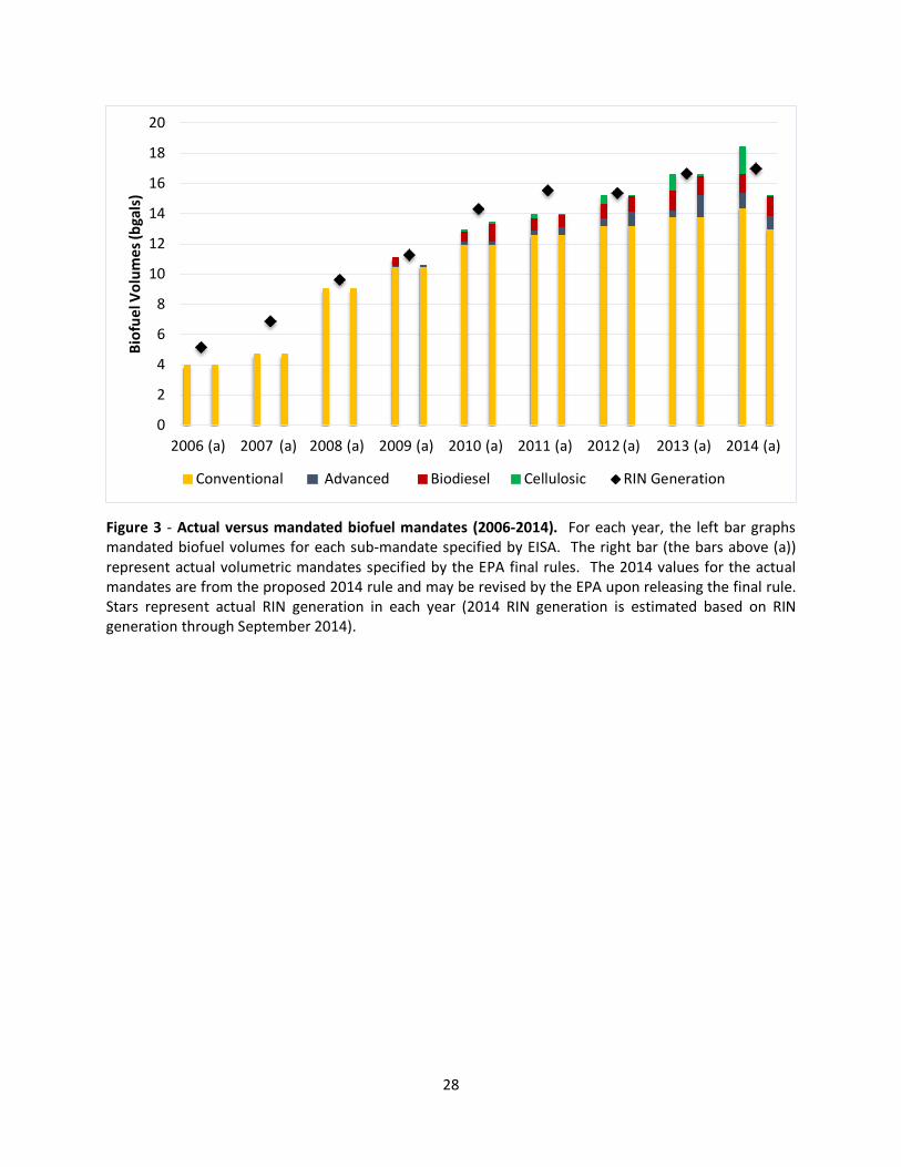
Figure 3 - Actual versus mandated biofuel mandates (2006-2014). For each year, the left bar graphs mandated biofuel volumes for each sub-mandate specified by EISA. The right bar (the bars above (a)) represent actual volumetric mandates specified by the EPA final rules. The 2014 values for the actual mandates are from the proposed 2014 rule and may be revised by the EPA upon releasing the final rule. Stars represent actual RIN generation in each year (2014 RIN generation is estimated based on RIN generation through September 2014).

0

2

4

6

8

10

12

14

16

18

20

2006 (a) 2007 (a) 2008 (a) 2009 (a) 2010 (a) 2011 (a) 2012 (a) 2013 (a) 2014 (a)

Biof

uel V

olum

es (b

gals

)

Conventional Advanced Biodiesel Cellulosic RIN Generation

28

(a) (b) (c)

(d) (e) (f)

29

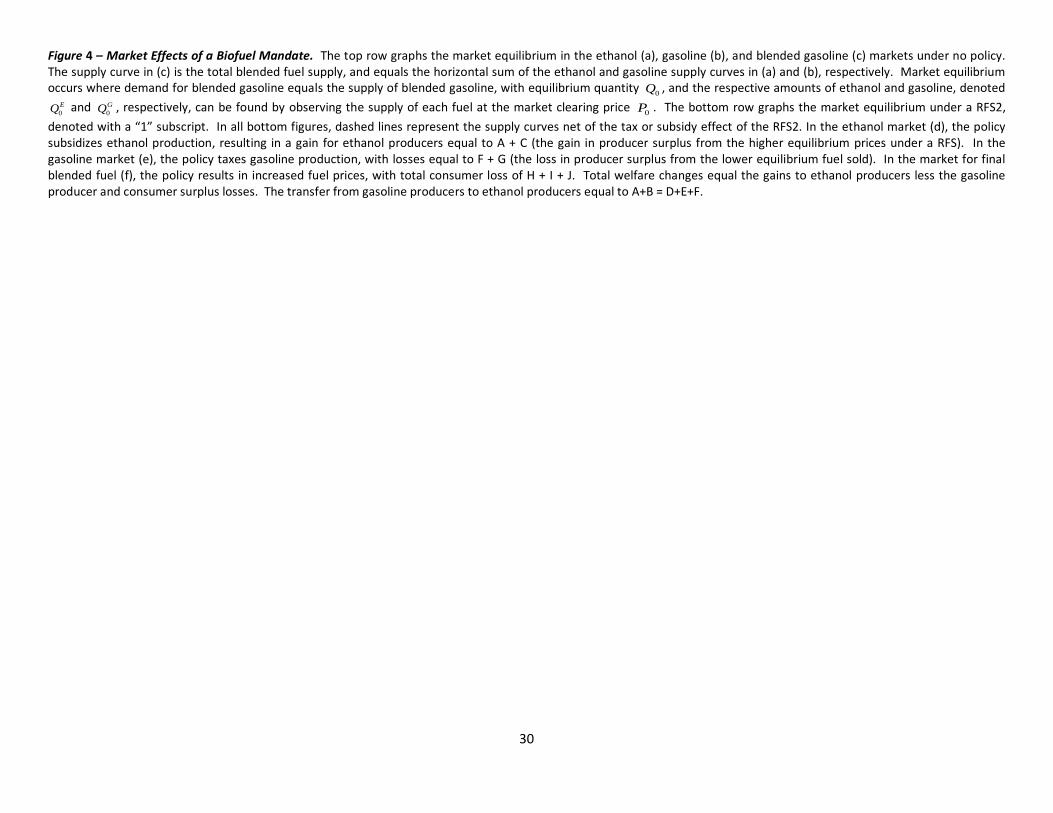
Figure 4 – Market Effects of a Biofuel Mandate. The top row graphs the market equilibrium in the ethanol (a), gasoline (b), and blended gasoline (c) markets under no policy. The supply curve in (c) is the total blended fuel supply, and equals the horizontal sum of the ethanol and gasoline supply curves in (a) and (b), respectively. Market equilibrium occurs where demand for blended gasoline equals the supply of blended gasoline, with equilibrium quantity 0Q , and the respective amounts of ethanol and gasoline, denoted

0EQ and 0

GQ , respectively, can be found by observing the supply of each fuel at the market clearing price 0P . The bottom row graphs the market equilibrium under a RFS2, denoted with a “1” subscript. In all bottom figures, dashed lines represent the supply curves net of the tax or subsidy effect of the RFS2. In the ethanol market (d), the policy subsidizes ethanol production, resulting in a gain for ethanol producers equal to A + C (the gain in producer surplus from the higher equilibrium prices under a RFS). In the gasoline market (e), the policy taxes gasoline production, with losses equal to F + G (the loss in producer surplus from the lower equilibrium fuel sold). In the market for final blended fuel (f), the policy results in increased fuel prices, with total consumer loss of H + I + J. Total welfare changes equal the gains to ethanol producers less the gasoline producer and consumer surplus losses. The transfer from gasoline producers to ethanol producers equal to A+B = D+E+F.

30

2022 Benefits and Costs of RFS2 Relative to 2007 AEO (billion $)

Category Lower Bound Upper Bound Overall Fuel Costs $11.8 $11.8 Energy Security $2.6 $2.6 Monetized Health Impacts ($2.2) ($0.63) Monetized GHG Impacts $0.60 $12.2 Total Yearly Net Calculated Benefits $12.8 $25.97 Other Quantified Costs Total Increase in Capital Costs through 2022 $90.5

$41.5 $3.6 $13

$0.51

Decreased Spending on Oil Imports Increased Farm Gate Food Expenditures Increase in Farm Income Decrease in Corn and Soybean Export Values Table 1 – EPA’s 2022 Cost-Benefit Summary. The table summarizes the net yearly benefits in 2022 of the RFS2 calculated in the EPA’s RIA for the primary RFS2 control case relative to the AEO 2007 reference case. Numbers in parentheses represent costs. The bottom portion of the table characterizes miscellaneous costs and benefits of the RFS2 calculated in the RIA that are not represented in the yearly cost-benefit calculation.

31

Figure 5 – AEO Projected Oil Prices. The figure graphs historical oil prices as well as 2007 and 2009 AEO oil price projects. We include high and low price projects from each AEO. As can be seen, the 2007 reference case is near the 2009 low price scenario, reflecting the large expected increases in 2009 AEO anticipated by the Energy Information Administration.

32

Fuel Costs ($/gal) Change in Average Gas Market Expenditures

($/gal) Year Gasoline Corn Ethanol Cellulosic Ethanol Imported Ethanol 2010 $1.57 $1.60 $2.20 $1.58 $0.003 2011 $1.91 $1.60 $2.03 $1.57 $0.004 2012 $2.18 $1.60 $1.86 $1.56 $0.005 2013 $2.41 $1.59 $1.68 $1.55 $0.005 2014 $2.62 $1.58 $1.51 $1.54 $0.005 2015 $2.83 $1.58 $1.34 $1.53 $0.001 2016 $2.97 $1.57 $1.33 $1.53 -$0.001 2017 $3.08 $1.56 $1.32 $1.52 -$0.007 2018 $3.20 $1.55 $1.31 $1.52 -$0.014 2019 $3.26 $1.54 $1.30 $1.52 -$0.019 2020 $3.30 $1.52 $1.29 $1.51 -$0.020 2021 $3.34 $1.51 $1.28 $1.51 -$0.020 2022 $3.35 $1.50 $1.27 $1.50 -$0.024

(a)

Fuel Costs ($/gal) Change in Average Diesel Market Expenditures

($/gal) Year Diesel Biodiesel Cellulosic Diesel Renewable Diesel 2010 $1.54 $2.61 $2.58 $2.36 $0.013 2011 $1.98 $2.64 $2.56 $2.36 $0.011 2012 $2.32 $2.27 $2.55 $2.36 $0.006 2013 $2.62 $2.27 $2.53 $2.38 $0.002 2014 $2.88 $2.25 $2.51 $2.40 -$0.004 2015 $3.15 $2.26 $2.49 $2.43 -$0.014 2016 $3.33 $2.28 $2.48 $2.45 -$0.024 2017 $3.47 $2.32 $2.46 $2.47 -$0.035 2018 $3.62 $2.34 $2.44 $2.46 -$0.050 2019 $3.69 $2.35 $2.42 $2.45 -$0.063 2020 $3.75 $2.38 $2.41 $2.44 -$0.078 2021 $3.80 $2.41 $2.39 $2.43 -$0.101 2022 $3.83 $2.44 $2.37 $2.42 -$0.120

(b)

Table 2 – EPA’s Fuel Market Impact Estimates. EPA estimated yearly per gallon costs of the RFS2 for gasoline and diesel.

33

Figure 6 – RIN Prices (04/2008-10/2014). The figure graphs monthly RIN prices using the current year RIN price for each type of RIN. Source: OPIS.

34

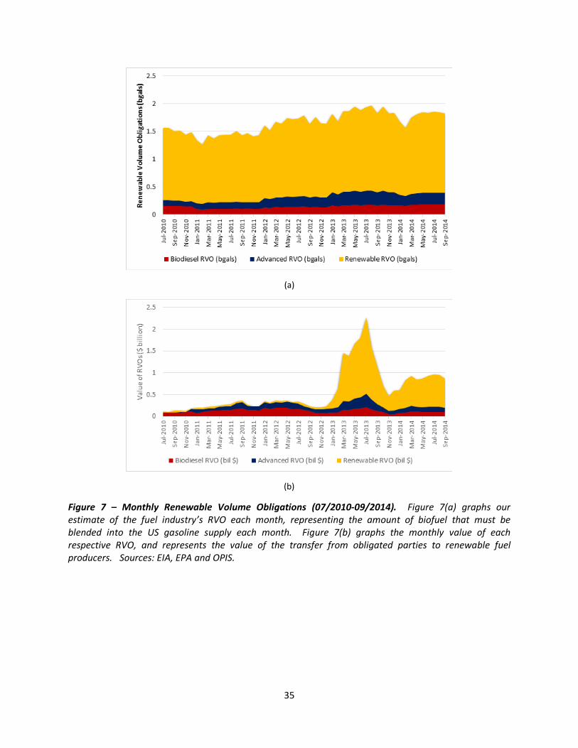
(a)

(b)

Figure 7 – Monthly Renewable Volume Obligations (07/2010-09/2014). Figure 7(a) graphs our estimate of the fuel industry’s RVO each month, representing the amount of biofuel that must be blended into the US gasoline supply each month. Figure 7(b) graphs the monthly value of each respective RVO, and represents the value of the transfer from obligated parties to renewable fuel producers. Sources: EIA, EPA and OPIS.

35

Figure 8 – Implicit value of the tax for each mandate under the RFS2. The values are calculated assuming full pass through of the implicit tax on gasoline and diesel to fuel prices. As shown in Lade, Lin and Smith (2015), the implicit tax is equal to the current year RIN price multiplied by the respective RFS2 standard for the year.

36

Conventional RIN

Tax Advanced RIN Tax Conventional + Advanced RIN Tax

EPA Gasoline Cost Estimates Biodiesel RIN Tax

EPA Diesel Cost Estimates

2010 $0.002 $0.001 $0.003 $0.003

$0.006 $0.013

($0.001, $0.003) ($0.000, $0.004) ($0.001, $0.007) ($0.005, $0.007) 2011 $0.002 $0.006 $0.008

$0.004 $0.009

$0.011 ($0.000, $0.003) ($0.004, $0.009) ($0.004, $0.012) ($0.006, $0.012)

2012 $0.003 $0.007 $0.010 $0.005

$0.010 $0.006

($0.001, $0.005) ($0.005, $0.010) ($0.006, $0.015) ($0.005, $0.014) 2013 $0.058 $0.011 $0.069

$0.005 $0.008

$0.002 ($0.013, $0.113) ($0.005, $0.019) ($0.018, $0.133) ($0.003, $0.014)

2014 $0.043 $0.007 $0.050 $0.005

$0.006 -$0.004

($0.030, $0.048) ($0.006, $0.008) ($0.036, $0.056) ($0.005, $0.008) Table 3- RIN Cost Estimates vs. EPA’s Ex Ante Cost Estimates. The table compares our ex post measure of wholesale gasoline and diesel costs to the EPA’s ex ante estimates of average gasoline and diesel market costs. Low and high prices are reported in parentheses. We assume above that the implicit tax from the conventional and advanced biofuel mandates predominantly affect gasoline markets, while the implicit tax from the biodiesel mandate affects diesel markets.

37

(a)

(b)

Figure 9 – Break-even ethanol and biodiesel prices.

38