Embed Size (px)
Citation preview
Stefano Nichele
Evolvability, Complexity and
Scalability of Cellular Evolutionary
and Developmental Systems
Thesis for the degree of Philosophiae Doctor
Trondheim, June 2014
Norwegian University of Science and Technology Faculty of Information Technology, Mathematics and
Electrical Engineering
Department of Computer and Information Science
NTNU - Trondheim Norwegian University of
Science and Technology
Copyright © 2014 Stefano Nichele
ISBN 978-82-326-0730-3 (printed version)
ISBN 978-82-326-0731-0 (electronic version)
ISSN 1503-8181
Doctoral theses at NTNU, 2015:31
Printed in Norway by NTNU-trykk, Trondheim
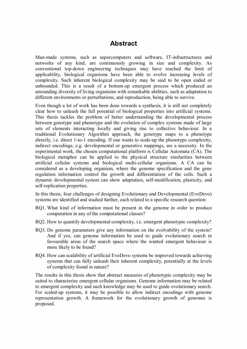
Abstract
Man-made systems, such as supercomputers and software, IT-infrastructures and
networks of any kind, are continuously growing in size and complexity. As
conventional top-down engineering techniques may have reached the limit of
applicability, biological organisms have been able to evolve increasing levels of
complexity. Such inherent biological complexity may be said to be open ended or
unbounded. This is a result of a bottom-up emergent process which produced an
astounding diversity of living organisms with remarkable abilities, such as adaptation to
different environments or perturbations, and reproduction, being able to survive.
Even though a lot of work has been done towards a synthesis, it is still not completely
clear how to unleash the full potential of biological properties into artificial systems.
This thesis tackles the problem of better understanding the developmental process
between genotype and phenotype and the evolution of complex systems made of large
sets of elements interacting locally and giving rise to collective behaviour. In a
traditional Evolutionary Algorithm approach, the genotype maps to a phenotype
directly, i.e. direct 1-to-1 encoding. If one wants to scale-up the phenotype complexity,
indirect encodings, e.g. developmental or generative mappings, are a necessity. In the
experimental work, the chosen computational platform is Cellular Automata (CA). The
biological metaphor can be applied to the physical structure similarities between
artificial cellular systems and biological multi-cellular organisms. A CA can be
considered as a developing organism, where the genome specification and the gene
regulation information control the growth and differentiation of the cells. Such a
dynamic developmental system can show adaptation, self-modification, plasticity, and
self-replication properties.
In this thesis, four challenges of designing Evolutionary and Developmental (EvoDevo)
systems are identified and studied further, each related to a specific research question:
RQ1. What kind of information must be present in the genome in order to produce
computation in any of the computational classes?
RQ2. How to quantify developmental complexity, i.e. emergent phenotypic complexity?
RQ3. Do genome parameters give any information on the evolvability of the system?
And if yes, can genome information be used to guide evolutionary search in
favourable areas of the search space where the wanted emergent behaviour is
more likely to be found?
RQ4. How can scalability of artificial EvoDevo systems be improved towards achieving
systems that can fully unleash their inherent complexity, potentially at the levels
of complexity found in nature?
The results in this thesis show that abstract measures of phenotypic complexity may be
suited to characterize emergent cellular organisms. Genome information may be related
to emergent complexity and such knowledge may be used to guide evolutionary search.
For scaled-up systems, it may be possible to allow indirect encodings with genome
representation growth. A framework for the evolutionary growth of genomes is
proposed.

iv
Preface
This doctoral thesis was submitted to the Norwegian University of Science and
Technology (NTNU) in partial fulfilment of the requirements for the degree of
philosophiae doctor (PhD). This doctoral work has been performed at the Department of
Computer and Information Science, NTNU, Trondheim, under the supervision of
Associate Professor Gunnar Tufte.
This PhD in Information Technology has been financed by the Faculty of Information
Technology, Mathematics and Electrical Engineering, NTNU, Trondheim.

vi
Acknowledgements
I would like to thank my supervisor Associate Professor Gunnar Tufte for his invaluable
support, advice and trust, but most of all for his uniqueness. Thanks for making me
discover this fantastic research world when I was an exchange student, thanks for
helping me as a master’s student, thanks once more for having me as a PhD student. I
cannot imagine a better supervisor.
I extend my gratitude to my co-supervisors Professor Helge Langseth and Adjunct
Associate Professor Jørn Amundsen for valuable feedback and encouragement during
the mid-term evaluation meetings. In addition, I would like to thank my colleagues in
the CARD group and in the entire Department of Computer and Information Science,
for having created such a stimulating and pleasant working environment.
Thanks to all my friends, those who live in Italy, those here in Norway and those all
around the world. Thanks for just being who you are.
All of this would not have been possible without the love of my parents. My deepest
gratitude goes to them, Ambrogina and Doriano, and my grandmother Giovanna.
Finally, thanks Ann-Marie for being the most important person of my life.
Stefano Nichele
June 06, 2014

viii
Contents
Abstract ................................................................................................................. iii
Preface .................................................................................................................... v
Acknowledgements ................................................................................................ vii
Contents ................................................................................................................. ix
List of Figures ........................................................................................................ xi
List of Tables ......................................................................................................... xi
Abbreviations ....................................................................................................... xii
1. Introduction ........................................................................................................ 1
Introduction 1 The Content of the Thesis 2
Research Questions 3 Thesis Outline 4
2. Background ......................................................................................................... 7
Artificial Development 7
Artificial Evolution 8 EvoDevo 9
Cellular Automata 10 Edge of Chaos and Genome Parameters 12
Genotype-to-Phenotype Encodings 14 Complexification 16
3. Research Summary........................................................................................... 19
Research Process 19
How the Ideas Developed 21 Category A 21
Category B 21 Category C 22
Category D 22 Category E 22
4. Research Results Summary .............................................................................. 25
Paper A.1 25
Abstract .......................................................................................................... 25 Roles of the Authors ....................................................................................... 26
Retrospective View ......................................................................................... 26 Paper A.2 26
x Contents
Abstract .......................................................................................................... 26
Roles of the Authors ....................................................................................... 26 Retrospective View ......................................................................................... 27
Paper B.1 27 Abstract .......................................................................................................... 27
Roles of the Authors ....................................................................................... 27 Retrospective View ......................................................................................... 28
Paper C.1 28 Abstract .......................................................................................................... 28
Roles of the Authors ....................................................................................... 28 Retrospective View ......................................................................................... 28
Paper C.2 29 Abstract .......................................................................................................... 29
Roles of the Authors ....................................................................................... 29 Retrospective View ......................................................................................... 30
Paper D.1 30 Abstract .......................................................................................................... 30
Roles of the Authors ....................................................................................... 31 Analysis Summary .......................................................................................... 31
Paper D.2 31 Abstract .......................................................................................................... 31
Roles of the Authors ....................................................................................... 32 Analysis Summary .......................................................................................... 32
Other Publications 33 Paper E.1 ........................................................................................................ 33
Paper E.2 ........................................................................................................ 33 Paper E.3 ........................................................................................................ 33
5. Concluding Remarks and Further Work ........................................................ 35
Conclusion 35
Contributions 36 Further Work 39
Bibliography ......................................................................................................... 41
Appendices ............................................................................................................ 49
Paper A.1 49 Paper A.2 59
Paper B.1 73 Paper C.1 89
Paper C.2 99 Paper D.1 113
Paper D.2 139
List of Figures
Figure 1: Example of development of an Italian Flag organism. .................................... 7
Figure 2: Trajectory and attractors of developmental systems (adapted from [84]). ....... 8
Figure 3: Graphical representation of a standard Genetic Algorithm. ............................. 9
Figure 4: Graphical representation of a Genetic Algorithm with Development. ........... 10
Figure 5: Chris Langton's schematic of rule space structure, with example space-time
behaviours (adapted from [40]). .......................................................................... 12
Figure 6: Location of the Wolfram classes in λ space (adapted from [36]). Class 4 is at a
phase transition between ordered and disordered dynamics.................................. 13
Figure 7: Example of direct mapping between genotype and phenotype. Each
connection between two nodes in the network is represented by a specific gene. . 15
Figure 8: Chronological Structure of Papers and Concepts .......................................... 20
Figure 9: Logical Structure of Papers and Concepts .................................................... 20
List of Tables
Table 1: Paper Categories ........................................................................................... 19
Table 2: Paper Category A .......................................................................................... 21
Table 3: Paper Category B .......................................................................................... 21
Table 4: Paper Category C .......................................................................................... 22
Table 5: Paper Category D .......................................................................................... 22
Table 6: Paper Category E........................................................................................... 23
xii Abbreviations
Abbreviations
AE Artificial Embryogeny
AI Artificial Intelligence
AL Artificial Life
CA Cellular Automaton
CC Cellular Computing
CGP Cartesian Genetic Programming
DS Development Step
EA Evolutionary Algorithm
EC Evolutionary Computation
EHW Evolvable HardWare
EvoDevo Evolutionary and Developmental (Systems)
FPGA Field-Programmable Gate Array
FSM Finite State Machine
GA Genetic Algorithm
GP Genetic Programming
GRN Gene Regulatory Network
IBD Instruction-Based Development
LUA Last Universal Ancestor
LZ77 Lempel-Ziv 1977
NEAT NeuroEvolution of Augmenting Topologies
RBN Random Boolean Network
RNN Recursive Neural Network
RQ Research Question
SMCGP Self-Modifying Cartesian Genetic Programming
Chapter 1 Introduction
"I must not fear. Fear is the mind-killer. Fear is the little-death
that brings total obliteration. I will face my fear. I will permit it
to pass over me and through me. And when it has gone past I will
turn the inner eye to see its path. Where the fear has gone there
will be nothing. Only I will remain."
--- Frank Herbert, Dune - Bene Gesserit Litany Against Fear
Introduction
Humans’ engineering abilities are remarkable. We managed to create a large amount of
artefacts and machines of increasing complexity. Yet, we did not succeed designing and
engineering behaviour and properties that are as complex as they appear in nature.
Biological organisms are an impressive example of very energy efficient massively-
parallel decentralized computation machines that emerge out of self-organization and
adaptation to different environments. Properties that we take for granted in biological
systems, such as reproduction, learning, and growth, are extremely hard to engineer and
design. Having those properties in man-made technology would revolutionize our way
of living and computing.
That is why there is a branch of computer science studies called bio-inspired
computation. Biologically-inspired techniques have been quite popular and (to some
degree) successful in recent years. Nevertheless, the complexity of the tackled problems
is not at the “nature level” of complexity. This is because the underlying mechanisms of
natural processes such as development and evolution are difficult to synthesize [37, 38]
with the same level of detail in computers.
The focus of this work is to better understand the underlying properties of artificial
development and artificial evolution with the goal of reducing the gap between the
natural and the artificial domain. This includes taking inspiration from nature and
biology towards artificial EvoDevo systems [23] that are capable to perform
computation.
The first part is devoted to the study of genome parameters, e.g. some quantification of
genotype properties, and their relation to the developed phenotypes. If the emergent
behaviour can be forecasted from the genotype, it may be possible to use such
information at the design stage of the system. Moreover, if solutions are to be found by
2 Introduction
evolution, such information may help guiding evolution in the vast search space, where
the sought behaviour is more likely to be found. This is related to the second part of the
thesis, which includes studies on evolvability and complexity. The last part of this thesis
tackles the problem of scalability. As in biological systems, genotype-to-phenotype
mapping allows a single cell to develop into a multi-cellular organism like the human
body, which consists of roughly 3.72x10¹³
cells. The “building instructions” included in
the DNA have a much smaller representation, estimated between 22 000 and 25 000
genes [5]. For artificial systems that target the development of phenotypes made of a
vast amount of components, it is not completely understood how to represent the
genotype. It is also not clear which size or which mapping to use, so that evolvability is
not annihilated, complexity is not bounded (open-ended evolution), and the genotype
representation can automatically scale if the phenotypic resources scale-up.
The Content of the Thesis
This thesis is at the intersection of several disciplines and research fields, which may be
grouped under the term “biologically-inspired computation”. That means borrowing
principles for biology and nature with the ultimate goal of building man-made systems
that exhibit behaviour characteristic of natural living systems, e.g. self-organization,
emergence, evolution, development, and ability to perform computation. Consequently,
the following concepts and theories are extensively used:
Evolutionary Design: process of generating designs (in the broader sense, e.g.
evolutionary search, evolutionary optimization, evolutionary artificial life) by
computers [3] by means of Darwinian evolution, i.e. evolution by natural selection;
Morphogenetic Engineering: modelling and implementation of “self-architecturing”
systems [17], inspired by biological morphogenesis and multi-cellular development
[35];
Complex Systems and Complexity Theory: emergence of collective behaviour out
of the local interaction of simple parts [1] and its quantification;
Complexification: incremental evolution of structured phenotypes, starting from
simple genomes, by systematic elaboration over generations by means of gene
addition [69];
Cellular Automata: mathematical and computational models (discrete dynamical
systems) for complex natural systems containing large numbers of simple
components, i.e. cells, which interact locally [81];
Artificial Life: the study of “life-as-it-could-be” [38], in contrast to biology that
studies “life-as-we-know-it”, based on the only kind of life available to study, i.e.
carbon-chain chemistry.

Research Questions 3
Research Questions
The main research question that is addressed in this thesis is:
How to apply artificial evolution and development for the design of cellular
machines that can produce complex computation and modelling?
This includes investigation of the relation between genotype and emergent phenotype in
EvoDevo systems with indirect encodings and how this is related to the complexity of
the mapping. In artificial life systems, a main challenge is how to specify input data, i.e.
system specifications and regulation mechanisms, and how to interpret the emergent
dynamics of the system, i.e. the output. In this context, cellular machines [66] are based
on three main principles: simplicity, vast parallelism, and locality. One example of
cellular computation machine [65] is Cellular Automata (CA).
In answering this main question, other research questions (RQs) have been addressed:
RQ1: What kind of information must be present in the genome in order to produce
computation in any of the computational classes?
In this context, computational classes [81] refer to distinct universality classes which
characterize CA computational behaviour. As such, this research question includes the
investigation of different genome parameters and their ability to forecast the emergent
developmental behaviour of cellular systems. In an EvoDevo system, the dynamics of
the developing organism can be traced down to the information and representation of
the genome and gene regulation. What information must be present? What information
processing capability must be available in the gene regulation? What cellular actions are
required to be expressed as to be able to develop a target organism? If a developmental
process is considered, the amount of regulatory information available to the
developmental process is crucial, e.g. number of cell types, local neighbourhoods, and
cellular actions such as growth, differentiation, and death.
RQ2: How to quantify developmental complexity, i.e. emergent phenotypic
complexity?
Since no universally accepted notion of complexity exists [33], many authors use it
implicitly without specifying which notion of complexity they are using. Yet, without
any common measure of developmental complexity, any significant claim may not be
verifiable. This study focuses on phenotypic complexity measures that take into account
the development process as a whole together with the phenotypic changes that occur,
e.g. trajectory, transient and attractor length. Moreover, this work investigates possible
measures of structural complexity, which take into account different emerging
structures and morphologies, e.g. Kolmogorov-based notions of complexity [41].
RQ3: Do genome parameters give any information on the evolvability of the system?
And if yes, can genome information be used to guide evolutionary search in
4 Introduction
favourable areas of the search space where the wanted emergent behaviour is
more likely to be found?
Evolvability is the ability of a system, e.g. a population of individuals, not only to create
genetic diversity but also to create such genetic variation that is able to adapt and
evolve. This means that it can produce beneficial variants that can be inherited by
natural selection. In an artificial EvoDevo system, evolvability cannot be taken for
granted. It is a property that depends on the chosen genotype representation and relative
genotype-to-phenotype mapping. Therefore this study investigates if genome
parameters can be an indicator of evolvability and whether they can be exploited
towards a balance between robustness and evolvability.
RQ4: How can scalability of artificial EvoDevo systems be improved towards
achieving systems that can fully unleash their inherent complexity, potentially at
the levels of complexity found in nature?
Evolutionary design targets systems of increasing complexity, built out of myriads of
components. Thus, indirect encodings and some kind of generative / developmental
system are often a necessity. Scaling-up the genotypes accordingly to the scaling-up of
phenotypes is an open challenge. For some systems, it would not be possible to fully
specify all the genotype regulations, due to the extremely high cardinality of
combinations. This makes it also infeasible to have a parameterization of the genotype
space for such systems. This study investigates how to fill this scalability gap, taking
inspiration from nature’s way of scaling, e.g. morphogenesis and gene duplication.
The described research questions are in tune with at least three points of the “Open
Problems in Artificial Life” [2]:
Explain how rules and symbols are generated from physical dynamics in living
systems;
Determine what is inevitable in the open-ended evolution in life;
Develop a theory of information processing, information flow, and information
generation for evolving systems.
Thesis Outline
This thesis contains an overview and a collection of papers. The main work and
contributions are in the enclosed papers. The overview of the thesis is organized as
follows:
Chapter 2 – theoretical background and related work. This chapter gives an
overview of the relevant research areas and describes the theoretical background on
which this thesis is based on.
Thesis Outline 5
Chapter 3 – research process with an explanation of how ideas and concepts
developed and their relation to the published work. This chapter describes the
logical and chronological connections to the developed ideas. Papers not included in
this thesis are also described.
Chapter 4 – research results summary. This chapter summarizes the results and
reviews the included papers (for the full papers see Appendices). The core
contribution of this thesis is represented by the described papers. For readability
purposes, the papers are summarized in this chapter.
Chapter 5 – concluding remarks and recommendations for further work. The last
chapter concludes the thesis by reviewing the research questions and given
contributions. It also describes the challenges and potential directions for future
work.
Appendices – collection of papers.

6
Chapter 2 Background
"I see no good reason why the views given in this volume should
shock the religious feelings of any one."
--- Charles Darwin, On the Origin of Species
Artificial Development
Artificial development is inspired by biological development, which is the complex
process that “builds” a multi-cellular organism starting from the “instructions” encoded
in the genome, the DNA. Since the sequencing of the human genome in 2001 [79],
considerable steps have been taken towards a better understanding of biological
morphogenesis. Development has many interesting features that may be convenient in
the artificial domain, such as the ability to shrink the representation of an adult
organism in a genetic plan which consists of a number of genes several orders of
magnitude smaller than the total number of cells in the developed organism [5].
Artificial development uses indirect encoding [68], in contrast to direct encodings where
there is a one-to-one mapping between the genotype and the phenotype. The different
genotype-to-phenotype encodings are explained in the remainder of this chapter.
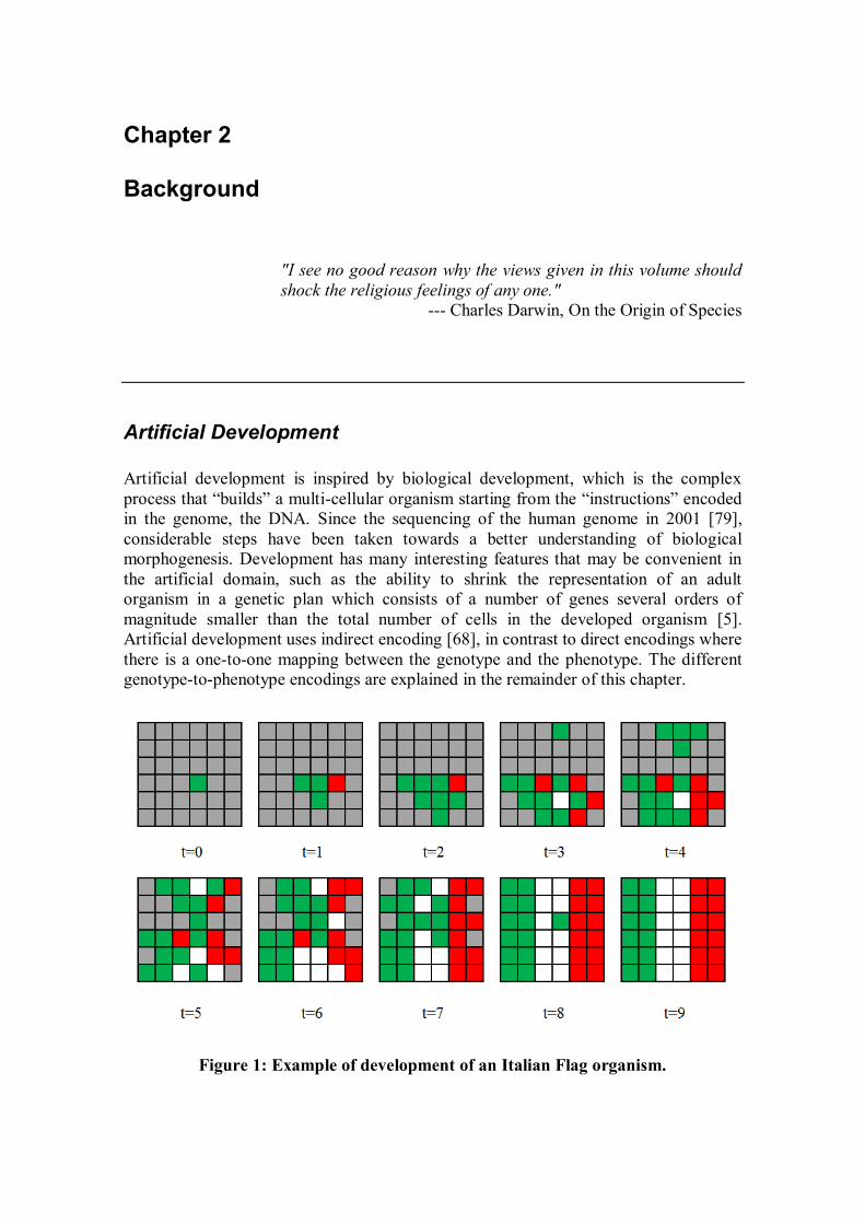
Figure 1: Example of development of an Italian Flag organism.
8 Background
Figure 1 gives an example of the development of an Italian Flag multi-cellular
organism. At time-step 1, only a single green cell, i.e. zygote, is placed in the centre of a
6 by 6 grid with cyclic boundary conditions. At each time-step the cellular world is
updated synchronously by following the developmental plan, i.e. transition table based
on neighbourhood (5 neighbours, von Neumann neighbourhood), which is present in
every cell. At time-step 9 the Italian Flag pattern has emerged out of local interactions
between cells and the structure remains stable afterwards, i.e. point attractor. In such a
system, each cell has no knowledge of the overall state of the system, i.e. there is no
central controller. The computation is purely based on local interactions between cells
based on each cell’s state and the neighbouring cell’s state. Several types of artificial
development exist. These are based on developmental rules [48, 65], generative
grammars [44, 31], or other morphogenetic mechanisms [17]. The actual computation
process is implemented in development steps, where cells can grow, differentiate and
die. More information on the developmental model in Figure 1 is given in [55].
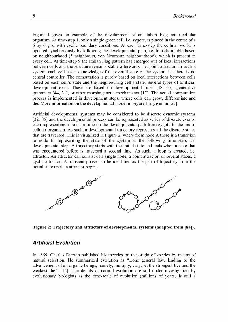
Artificial developmental systems may be considered to be discrete dynamic systems
[32, 85] and the developmental process can be represented as series of discrete events,
each representing a point in time on the developmental path from zygote to the multi-
cellular organism. As such, a developmental trajectory represents all the discrete states
that are traversed. This is visualized in Figure 2, where from node A there is a transition
to node B, representing the state of the system at the following time step, i.e.
developmental step. A trajectory starts with the initial state and ends when a state that
was encountered before is traversed a second time. As such, a loop is created, i.e.
attractor. An attractor can consist of a single node, a point attractor, or several states, a
cyclic attractor. A transient phase can be identified as the part of trajectory from the
initial state until an attractor begins.
Figure 2: Trajectory and attractors of developmental systems (adapted from [84]).
Artificial Evolution
In 1859, Charles Darwin published his theories on the origin of species by means of
natural selection. He summarized evolution as “...one general law, leading to the
advancement of all organic beings, namely, multiply, vary, let the strongest live and the
weakest die.” [12]. The details of natural evolution are still under investigation by
evolutionary biologists as the time-scale of evolution (millions of years) is still a
EvoDevo 9
challenge for direct experimentation. In computer experiments, evolution can be carried
out in a realistic time and the main ideas have been applied successfully in several
disciplines, such as the evolution of robot controllers [58], design of antennas [29], and
many more [47, 20, 25]. In the computer context, evolution is referred to as
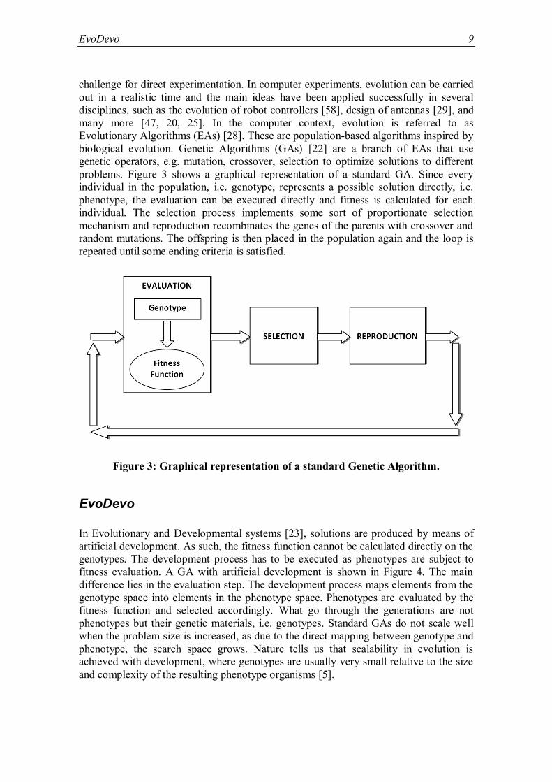
Evolutionary Algorithms (EAs) [28]. These are population-based algorithms inspired by
biological evolution. Genetic Algorithms (GAs) [22] are a branch of EAs that use
genetic operators, e.g. mutation, crossover, selection to optimize solutions to different
problems. Figure 3 shows a graphical representation of a standard GA. Since every
individual in the population, i.e. genotype, represents a possible solution directly, i.e.
phenotype, the evaluation can be executed directly and fitness is calculated for each
individual. The selection process implements some sort of proportionate selection
mechanism and reproduction recombinates the genes of the parents with crossover and
random mutations. The offspring is then placed in the population again and the loop is
repeated until some ending criteria is satisfied.
Figure 3: Graphical representation of a standard Genetic Algorithm.
EvoDevo
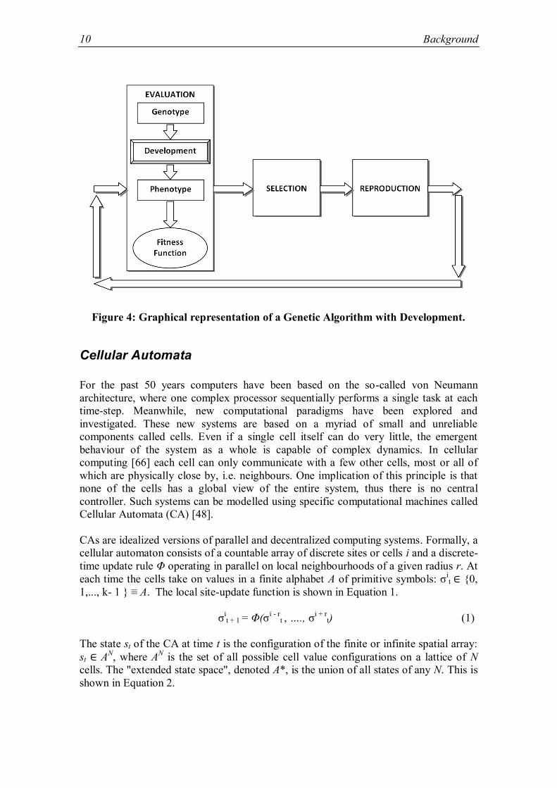
In Evolutionary and Developmental systems [23], solutions are produced by means of
artificial development. As such, the fitness function cannot be calculated directly on the
genotypes. The development process has to be executed as phenotypes are subject to
fitness evaluation. A GA with artificial development is shown in Figure 4. The main
difference lies in the evaluation step. The development process maps elements from the
genotype space into elements in the phenotype space. Phenotypes are evaluated by the
fitness function and selected accordingly. What go through the generations are not
phenotypes but their genetic materials, i.e. genotypes. Standard GAs do not scale well
when the problem size is increased, as due to the direct mapping between genotype and
phenotype, the search space grows. Nature tells us that scalability in evolution is
achieved with development, where genotypes are usually very small relative to the size
and complexity of the resulting phenotype organisms [5].
10 Background
Figure 4: Graphical representation of a Genetic Algorithm with Development.
Cellular Automata
For the past 50 years computers have been based on the so-called von Neumann
architecture, where one complex processor sequentially performs a single task at each
time-step. Meanwhile, new computational paradigms have been explored and
investigated. These new systems are based on a myriad of small and unreliable
components called cells. Even if a single cell itself can do very little, the emergent
behaviour of the system as a whole is capable of complex dynamics. In cellular
computing [66] each cell can only communicate with a few other cells, most or all of
which are physically close by, i.e. neighbours. One implication of this principle is that
none of the cells has a global view of the entire system, thus there is no central
controller. Such systems can be modelled using specific computational machines called
Cellular Automata (CA) [48].
CAs are idealized versions of parallel and decentralized computing systems. Formally, a
cellular automaton consists of a countable array of discrete sites or cells i and a discrete-
time update rule Φ operating in parallel on local neighbourhoods of a given radius r. At
each time the cells take on values in a finite alphabet A of primitive symbols: σit ∈ {0,
1,..., k- 1 } ≡ A. The local site-update function is shown in Equation 1.
σit + 1 = Φ(σ
i - rt , …., σ
i + rt) (1)
The state st of the CA at time t is the configuration of the finite or infinite spatial array:
st ∈ AN, where A
N is the set of all possible cell value configurations on a lattice of N
cells. The "extended state space", denoted A*, is the union of all states of any N. This is
shown in Equation 2.
Cellular Automata 11
A* = UN≥0 AN with A
0 = ∅ (2)
The CA global update rule Φ: AN → A
N applies Φ in parallel to all sites in the lattice: st
= Φ st - 1. For finite N it is also necessary to specify a boundary condition. The boundary
cells are dealt with by having the whole lattice wrap around into a torus, thus boundary
cells are connected to “adjacent" cells on the opposite boundary. The metaphor with
biology can be exploited on CAs because the physical structure is similar to biological
multi-cellular organisms. For this reason, CA can also be used to abstract and simulate a
biological developmental process [18, 61].
John von Neumann [80] studied the first cellular automaton in the 1940s, as an abstract
model of self-reproduction of machines inspired by biology [82]. With the contribution
of Stanislaw Ulam [78], he defined a 29 state 2D CA that was able to self-replicate. In
the 1960s, research on cellular automata was conducted through analysis of variations
produced by a single automaton. For example, between 1960 and 1970, John Conway’s
Game of Life automaton [4] was introduced and studied extensively to understand the
behaviour of specific CA rules capable of complex dynamics. Later in 1980s, Stephen
Wolfram demonstrated that one-dimensional cellular automata could be sufficient to
investigate the totality of behaviour of CA rules. Instead of studying single CA rules, he
grouped rules producing similar behaviour and studied different classes depending on
the emergent patterns [81]. Wolfram identified four different computational classes:
Class 1 - fixed: CA development leads to a homogeneous state. Almost all initial
configurations relax after a transient period to the same fixed configuration. In this
class, the outcome of development is determined with probability 1, independently
on the initial state. The process is not reversible because all previous information is
lost.
Class 2 - cyclic: CA development leads to a set of stable and periodic structures.
Almost all initial configurations relax after a transient period to a fixed point or a
temporarily periodic cycle of configurations, which is dependent on the initial
configuration. Some parts of the initial configuration are filtered out and others are
propagated forever. The process is not reversible because information is partially
lost during development.
Class 3 - chaotic: CA development leads to a chaotic pattern. Almost all initial
configurations relax after a transient period to chaotic behaviour. The development
process is completely reversible since the previous state can be predicted from the
current state, i.e. chaotic behaviour is not random.
Class 4 - complex: CA development leads to complex localized structures,
sometimes long-lived. Information is propagated by the automaton at variable speed.
The process is non-reversible as the current site values could have arisen from more
than one previous configuration. This is the only class that contains non-trivial
automata.
All different cellular automata can be associated with one of the previous classes. In
practice, with finite lattices, there is only a finite number of possible configurations and
all rules lead to periodic behaviour. However, in theory the lattice is supposed to be
12 Background
infinite. The number of possible CA configurations grows exponentially with the
increase of CA size and number of cell types. For example, whilst a 1D CA of size 16
and 2 cell types has 216
(=65536) possible states, a 2 dimensional CA of size 16 by 16
and 3 cell types has 3256
(~1.39x10122
) possible states.
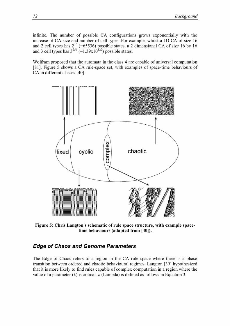
Wolfram proposed that the automata in the class 4 are capable of universal computation
[81]. Figure 5 shows a CA rule-space set, with examples of space-time behaviours of
CA in different classes [40].
Figure 5: Chris Langton's schematic of rule space structure, with example space-
time behaviours (adapted from [40]).
Edge of Chaos and Genome Parameters
The Edge of Chaos refers to a region in the CA rule space where there is a phase
transition between ordered and chaotic behavioural regimes. Langton [39] hypothesized
that it is more likely to find rules capable of complex computation in a region where the
value of a parameter (λ) is critical. λ (Lambda) is defined as follows in Equation 3.
Edge of Chaos and Genome Parameters 13
tot
q1 (3)
A quiescent state q has to be chosen, which is usually the state representing the empty
or dead state. In Equation 3, the ratio (q/tot) represents the fraction of “non-quiescent”
states in the rule-table used for CA development. When λ is equal to zero, all the rules
lead to a quiescent state and when λ is equal to Equation 4, the rule-table is the most
heterogeneous (k represents the number of different possible states of a cell).
k
11 (4)
Traversing λ from 0 to 1-1/k, it is possible to observe all the CA behaviour described by
the Wolfram classes, from ordered behaviour to chaotic behaviour. For certain λ critical
values, the CA tend to show complex and long-lived patterns as in Wolfram’s class 4.
Langton [39] hypothesized that Wolfram’s class 4, the only one with CA capable of
universal computation, is located somewhere around this critical value of λ, at the Edge
of Chaos. It may be said that in such a region the basic conditions to support
computation, i.e. information transmission, storage and modification, are most likely
present [39]. Langton studied entropy as a measure of the information carried by each
cell during the CA development and mutual information between a cell and itself at the
next time step. His research supports the hypothesis that for λ values in the proximity of
phase transitions, it is more likely to have well balanced conditions to support
computation [39]. For example, information storage involves low entropy. On the other
hand, information transmission requires increasing entropy. If a system needs to have
both in order to perform computation, there must be a trade-off as it may happen in the
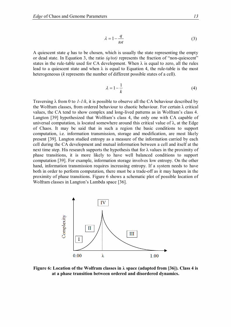
proximity of phase transitions. Figure 6 shows a schematic plot of possible location of
Wolfram classes in Langton’s Lambda space [36].
Figure 6: Location of the Wolfram classes in λ space (adapted from [36]). Class 4 is
at a phase transition between ordered and disordered dynamics.
14 Background
Besides Lambda, other genome parameters have been previously proposed. A
neighbourhood dependent parameter was presented by De Oliveira [14] under the name
Absolute Activity. Li [42] introduced Mean Field Parameters which monitor if the
majority of the regulatory actions follow the “mean” configuration. De Oliveira [14]
presented a very similar parameter called Neighbourhood Dominance. Binder [8, 9]
introduced the Sensitivity parameter which measures the number of changes in the
output of the transition table based on a change in the neighbourhood, one cell at a time,
over all the possible neighbourhoods of the rule being considered. This has also been
studied by De Oliveira [13, 14] under the name of Context Dependence. Wuensche [83]
defined the Z parameter, derived from a pre-image calculation algorithm in the state-
space. Different genome parameters have been shown to have specific abilities to
characterize the CA rule space. However, most of the literature deals with 1-
dimensional two-state CA.
Genotype-to-Phenotype Encodings
In the field of Evolutionary Computation (EC), each problem is represented as a
genotype and a specific fitness function is designed to evaluate qualities of the wanted
solutions. Evolutionary Algorithms (EAs) often use a one-to-one genotype-to-
phenotype mapping, which means that a candidate solution generated by the EA can be
directly mapped to the medium the solution was designed for. As such, each property
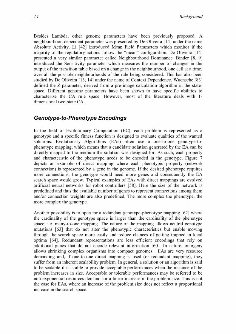
and characteristic of the phenotype needs to be encoded in the genotype. Figure 7
depicts an example of direct mapping where each phenotypic property (network
connection) is represented by a gene in the genome. If the desired phenotype requires
more connections, the genotype would need more genes and consequently the EA
search space would grow. Typical examples of EAs with direct mappings are evolved
artificial neural networks for robot controllers [58]. Here the size of the network is
predefined and thus the available number of genes to represent connections among them
and/or connection weights are also predefined. The more complex the phenotype, the
more complex the genotype.
Another possibility is to open for a redundant genotype-phenotype mapping [62] where
the cardinality of the genotype space is larger than the cardinality of the phenotype
space, i.e. many-to-one mapping. The nature of the mapping allows neutral genotype
mutations [63] that do not alter the phenotypic characteristics but enable moving
through the search space more easily and reduce chances of getting trapped in local
optima [64]. Redundant representations are less efficient encodings that rely on
additional genes that do not encode relevant information [60]. In nature, ontogeny
allows shrinking complex organisms into compact genomes. EAs are very resource
demanding and, if one-to-one direct mapping is used (or redundant mapping), they
suffer from an inherent scalability problem. In general, a solution or an algorithm is said
to be scalable if it is able to provide acceptable performances when the instance of the
problem increases in size. Acceptable or tolerable performances may be referred to be
non-exponential resources demand for a linear increase in the problem size. This is not
the case for EAs, where an increase of the problem size does not reflect a proportional
increase in the search space.
Genotype-to-Phenotype Encodings 15
Figure 7: Example of direct mapping between genotype and phenotype. Each
connection between two nodes in the network is represented by a specific gene.
One solution for the resource-demanding nature of EAs is to take inspiration from
nature and somehow shrink the genotype, i.e. indirect mapping. This reduces the overall
complexity of the genotype (and the search space magnitude) while adding more
complexity to the genotype-to-phenotype mapping and the underlying development
process. Thus the challenges are finding an efficient developmental mechanism and a
suitable indirect representation that is able to exploit such a development process.
Even though developmental systems are widely used [75, 16, 47, 30, 68], the genotype
representation scalability challenge still exists. For several developmental systems it
would not be feasible to represent all the possible regulatory combinations in the
genotype, e.g. complete regulatory information for Tufte’s CA based model [74] would
require the specification of 545 regulatory possibilities, Miller and Banzhaf’s cellular
developmental Cartesian Genetic Programming (CGP) model [47] a total of 7689, von
Neumann’s universal constructor [48] 295 combinations. For many systems, using
fixed-length genotypes, i.e. a subset of all the possible regulatory combinations, is a
necessity. In cellular models the total possible number of regulatory combinations is NK,
where N is the number of possible states each cell can hold and K is the neighbourhood.
Bidlo [7] had an instruction-based cellular model with 4 possible cell states and
neighbourhood of size 5 which used a restricted transition function of only 10 entries,
Tufte [73] had a model with 13 possible cell states and 5 neighbours whether the
available regulatory rule-set was restricted to 64. Tufte and Thomassen [77] investigated
scaling of genomes with fixed-length representation and allowed 4, 5, 6 and 32
regulation rules out of the possible regulatory information based on 3 cell types and 5
neighbours (13 cell types for genome of size 32). In all such cases, the maximum
representation was pre-defined and could not change during evolution. The available
regulatory information was designed a priori by trial and error or by estimation and did
16 Background
not guarantee that a possible solution could be found at all or that the same solutions
could be achieved with a smaller genotype representation. Moreover, the maximum
complexity of the system was predetermined, in the sense that the reachable search
space was shrunk by the chosen representation. If one wanted to scale-up the system by
allowing a larger neighbourhood or more available cell states, the chosen representation
may not be large enough to accommodate solutions anymore.
Complexification
Biological organisms are the best example of scalability, ranging from simple
unicellular to multi-cellular organisms, where trillions of cells develop from a single
cell which holds the complete genome. Roughly 3Gb of information is required to
encode the necessary base pairs for a fully sequenced human genome [79]. Obviously,
the optimization of the genetic plan is the result of evolution by natural selection. The
means of genome optimization are genetic operators, e.g. mutation, crossover. However,
genomes of different species have different lengths. There is scientific evidence that all
species have evolved and diverged from a common ancestor [72] [70], i.e. last universal
ancestor (LUA), which was most likely a unicellular organism that has lived some 3.5
to 3.8 billion years ago [15] [21]. The mechanism of gene duplication [71] played an
important role in genome expansion through evolution. This process allowed the
addition of new genes to offspring genomes. In fact, some parental genes are not only
copied but duplicated more than once. This leads to an offspring with larger genome
than the parents, which allows genetic novelty and potential evolutionary innovation
[59]. When a gene is duplicated, it creates a redundant gene with less selection pressure.
This means that the duplicated gene can undergo mutations without having deleterious
effects and eventually lead to a new functionality which produces an increase in fitness.
The natural and biological process of incremental genome growth and elaboration [46]
is known as complexification. Complexification through gene duplication is a plausible
explanation of how compact, efficient and robust genomes have evolved and solved an
inherent scalability issue, such as the representation of a complex multi-cellular
organism in a simpler and shorter genetic plan, which allows morphogenesis.
Martin [46] investigated the impact of gene duplication in the origin of vertebrates. He
claimed that such a duplication process produced an increased genome complexity
before the origin of fish. Such duplication events happened at relatively high rates.
Moreover, not only beneficial duplications become fixed in the genome but also neutral
duplications with respect to fitness. In some cases, when the original gene faces
negative mutations, the duplicated gene becomes also fixed. Key factors for gene
expansion by gene duplication and optimization are then mutation and fixation. Zhang
[86] studied the process of acquisition of new functions in duplicated genes. He argued
that gene duplication is an extremely important factor for evolution, providing new
genetic material for evolution to exploit by mutation, drift and selection, which leads to
new gene functions or specialization of existing ones. In fact, in the three domains of
life, i.e. bacteria, archaea and eukarya, there is strong evidence that large portions of
genes appeared by gene duplication (data from sequenced genomes). As an example,
around 38% of the Homo Sapiens genome is the result of gene duplication [43] and
Complexification 17
around 1800 duplication events took place since humans diverged from chimpanzees in
roughly 6 million years. This produces evidence that such a mechanism contributes to
plasticity / adaptation to changing environments and speciation, as well as the
emergence of complex regulatory mechanisms in gene regulatory networks.
Yet, the same degree of scalability, evolvability and complexity is not achieved in
evolved artificial developmental systems, partly because of the intricate genotype-to-
phenotype mapping and relative encoding (direct encoding or fixed-length encoding),
that leads to an extremely high dimensionality of the search space. Moreover, with
direct encodings this incremental approach is difficult to achieve because each gene
maps to a specific phenotypic functionality/structure and duplicating it would result in
significant alterations of the phenotype [67]. It may be argued that in order to retain the
advantages of biological complexification, it is necessary to exploit indirect encodings,
where duplication would not have a disruptive effect. Newly added genes, once
incorporated in the genome, would have time to be gradually modified without too
severe consequences on development and eventually being optimized.
An alternative that can scale both genotype and phenotype information is to allow a
variable length genome. If a mechanism of adding genes through gene duplication is
allowed, it is possible to grow the genome size incrementally. This complexification
strategy may help to solve the genotype representation scalability problem. Previous
work done towards achieving genome size expansion includes [11], [27], [34], [45].
Federici and Downing [19] investigated neutral gene duplication in a cellular model
with environmental chemicals. They studied genome scalability with direct encoding
and embryonal stages, using a gene regulatory model based on recursive neural
networks (RNN). Stanley and Miikkulainen [69] introduced NeuroEvolution of
Augmenting topologies (NEAT), a complexification method for the incremental
evolution of neural network architectures. Their main goal was to evolve robot
controllers with direct encodings through gene duplication. They argued that
incremental evolution of complex neural network genomes relies on three main
technical components: meaningful crossover by means of historical markings for gene
alignment, innovation through speciation which enables optimization, start from
minimal genomes and allow incremental increase is size. Research on complexification
of developmental systems with direct encodings may not be conclusive, but the basic
idea regarding incremental evolution of genome representations have the potential for
exploration with indirect encodings [67], where nature-like levels of complexity are
targeted. This would allow starting from simple potential solutions in a low dimensional
space and incrementally increasing the genotype complexity, disregarding how large a
genotype would be to encode a solution.

18
Chapter 3 Research Summary
"It was the best of times, it was the worst of times."
--- Charles Dickens, A Tale of Two Cities
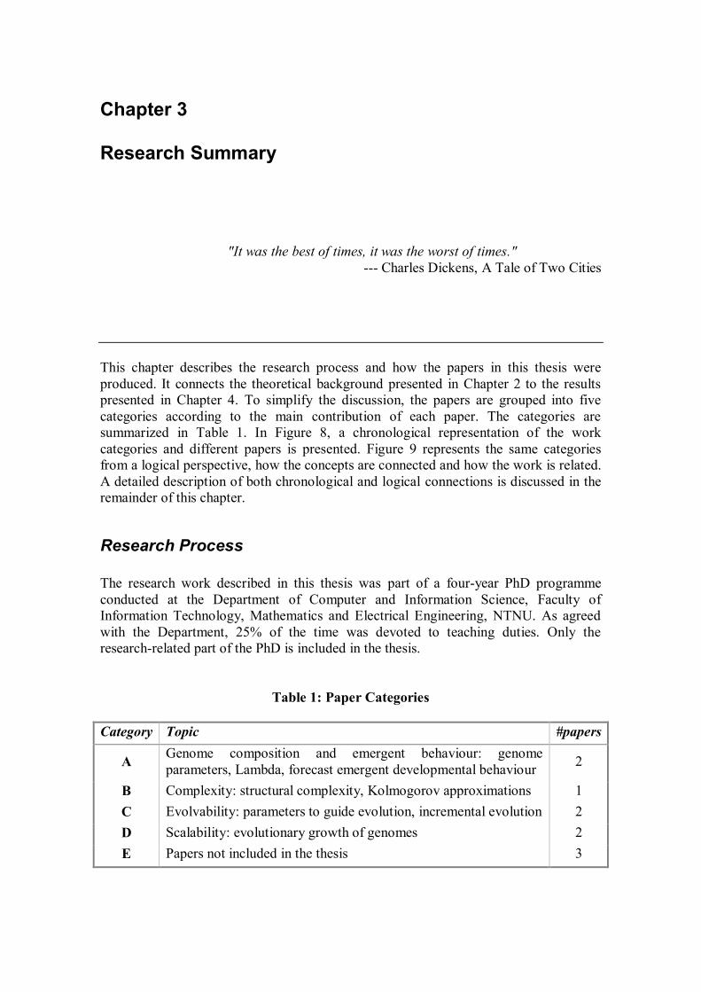
This chapter describes the research process and how the papers in this thesis were
produced. It connects the theoretical background presented in Chapter 2 to the results
presented in Chapter 4. To simplify the discussion, the papers are grouped into five
categories according to the main contribution of each paper. The categories are
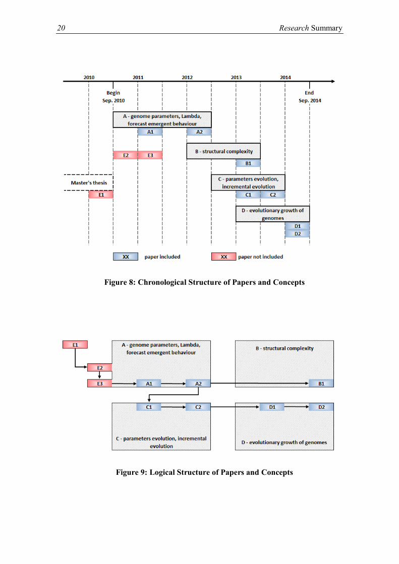
summarized in Table 1. In Figure 8, a chronological representation of the work
categories and different papers is presented. Figure 9 represents the same categories
from a logical perspective, how the concepts are connected and how the work is related.
A detailed description of both chronological and logical connections is discussed in the
remainder of this chapter.
Research Process
The research work described in this thesis was part of a four-year PhD programme
conducted at the Department of Computer and Information Science, Faculty of
Information Technology, Mathematics and Electrical Engineering, NTNU. As agreed
with the Department, 25% of the time was devoted to teaching duties. Only the
research-related part of the PhD is included in the thesis.
Table 1: Paper Categories
Category Topic #papers
A Genome composition and emergent behaviour: genome
parameters, Lambda, forecast emergent developmental behaviour 2
B Complexity: structural complexity, Kolmogorov approximations 1
C Evolvability: parameters to guide evolution, incremental evolution 2
D Scalability: evolutionary growth of genomes 2
E Papers not included in the thesis 3
20 Research Summary
Figure 8: Chronological Structure of Papers and Concepts
Figure 9: Logical Structure of Papers and Concepts
How the Ideas Developed 21
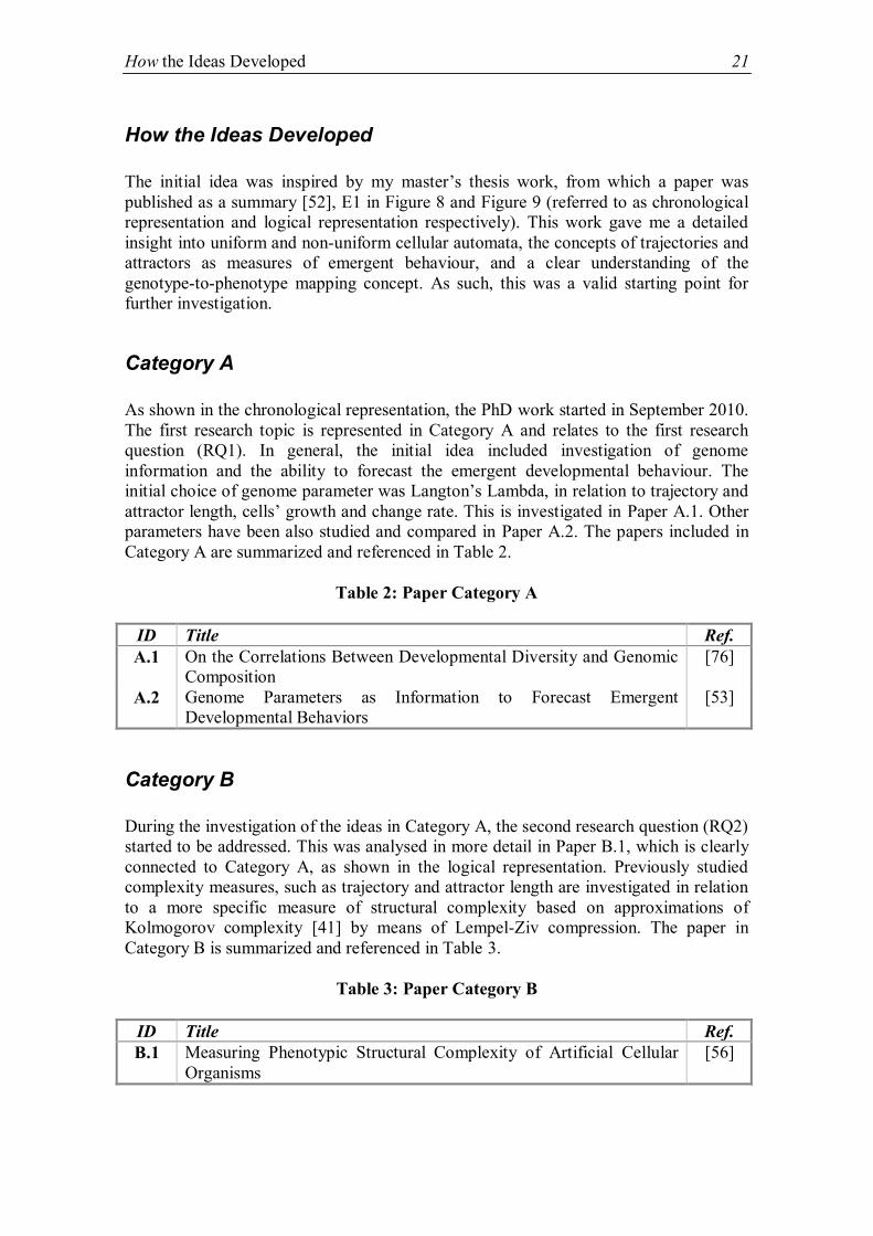
How the Ideas Developed
The initial idea was inspired by my master’s thesis work, from which a paper was
published as a summary [52], E1 in Figure 8 and Figure 9 (referred to as chronological
representation and logical representation respectively). This work gave me a detailed
insight into uniform and non-uniform cellular automata, the concepts of trajectories and
attractors as measures of emergent behaviour, and a clear understanding of the
genotype-to-phenotype mapping concept. As such, this was a valid starting point for
further investigation.
Category A
As shown in the chronological representation, the PhD work started in September 2010.
The first research topic is represented in Category A and relates to the first research
question (RQ1). In general, the initial idea included investigation of genome
information and the ability to forecast the emergent developmental behaviour. The
initial choice of genome parameter was Langton’s Lambda, in relation to trajectory and
attractor length, cells’ growth and change rate. This is investigated in Paper A.1. Other
parameters have been also studied and compared in Paper A.2. The papers included in
Category A are summarized and referenced in Table 2.
Table 2: Paper Category A
ID Title Ref.
A.1 On the Correlations Between Developmental Diversity and Genomic
Composition
[76]
A.2 Genome Parameters as Information to Forecast Emergent
Developmental Behaviors
[53]
Category B
During the investigation of the ideas in Category A, the second research question (RQ2)
started to be addressed. This was analysed in more detail in Paper B.1, which is clearly
connected to Category A, as shown in the logical representation. Previously studied
complexity measures, such as trajectory and attractor length are investigated in relation
to a more specific measure of structural complexity based on approximations of
Kolmogorov complexity [41] by means of Lempel-Ziv compression. The paper in
Category B is summarized and referenced in Table 3.
Table 3: Paper Category B
ID Title Ref.
B.1 Measuring Phenotypic Structural Complexity of Artificial Cellular
Organisms
[56]
22 Research Summary
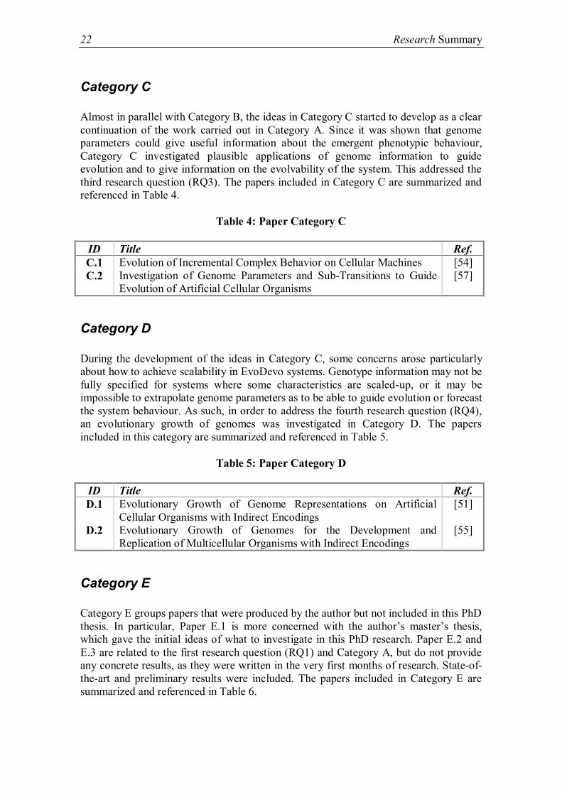
Category C
Almost in parallel with Category B, the ideas in Category C started to develop as a clear
continuation of the work carried out in Category A. Since it was shown that genome
parameters could give useful information about the emergent phenotypic behaviour,
Category C investigated plausible applications of genome information to guide
evolution and to give information on the evolvability of the system. This addressed the
third research question (RQ3). The papers included in Category C are summarized and
referenced in Table 4.
Table 4: Paper Category C
ID Title Ref.
C.1 Evolution of Incremental Complex Behavior on Cellular Machines [54]
C.2 Investigation of Genome Parameters and Sub-Transitions to Guide
Evolution of Artificial Cellular Organisms
[57]
Category D
During the development of the ideas in Category C, some concerns arose particularly
about how to achieve scalability in EvoDevo systems. Genotype information may not be
fully specified for systems where some characteristics are scaled-up, or it may be
impossible to extrapolate genome parameters as to be able to guide evolution or forecast
the system behaviour. As such, in order to address the fourth research question (RQ4),
an evolutionary growth of genomes was investigated in Category D. The papers
included in this category are summarized and referenced in Table 5.
Table 5: Paper Category D
ID Title Ref.
D.1 Evolutionary Growth of Genome Representations on Artificial
Cellular Organisms with Indirect Encodings
[51]
D.2 Evolutionary Growth of Genomes for the Development and
Replication of Multicellular Organisms with Indirect Encodings
[55]
Category E
Category E groups papers that were produced by the author but not included in this PhD
thesis. In particular, Paper E.1 is more concerned with the author’s master’s thesis,
which gave the initial ideas of what to investigate in this PhD research. Paper E.2 and
E.3 are related to the first research question (RQ1) and Category A, but do not provide
any concrete results, as they were written in the very first months of research. State-of-
the-art and preliminary results were included. The papers included in Category E are
summarized and referenced in Table 6.

Category E 23
Table 6: Paper Category E
ID Title Ref.
E.1 Trajectories and Attractors as Specification for the Evolution of
Behavior in Cellular Automata
[52]
E.2 Discrete Dynamics of Cellular Machines: Specification and
Interpretation
[49]
E.3 On the Edge of Chaos and Possible Correlations Between Behavior
and Cellular Regulative Properties
[50]

24
Chapter 4 Research Results Summary
"Second star to the right, and then straight on ‘til morning."
--- J. M. Barrie, Peter Pan
This chapter provides an overview of the papers included in this thesis, where and when
they were published. The included papers are discussed in Sections A.1 through E.3.
Each section contains the abstract of the paper and a description of the main
contribution of the different co-authors. When relevant, the sections also include a
discussion about how the work is seen in retrospective. The new papers D.1 and D.2 are
very recent and do not include a real retrospective view. As such, a paper description
with a state-of-the-art analysis is given. Finally, Section E lists the papers that are not
included in this thesis.
Paper A.1
On the Correlations Between Developmental Diversity and Genomic Composition
G. Tufte and S. Nichele
13th
Annual Genetic and Evolutionary Computation Conference, GECCO
ACM 2011
Abstract
In this work we target to measure genomic properties in EvoDevo systems so as to
predict phenotypic properties related to the emergence of artificial organisms. We
propose a measurement, λd, based on the composition of the genome, which can give
prediction of how the emerging organism will develop. The experimental approach uses
a minimalistic developmental model. The results show that the parameter λd can predict
phenotypic properties. The aim of introducing a parameter like λd is to get more
knowledge on the relation between genomic properties and phenotypic properties of
developing organisms.
26 Research Results Summary
Roles of the Authors
I contributed to the formulation of the initial idea proposed by Tufte. I also ran all the
simulations and proposed the experimental setup, tested the results, and analysed the
data. Tufte contributed through supervision and wrote most of the paper. I wrote parts
of the paper, provided feedback and corrections.
Retrospective View
This paper continued the preliminary work started in [49] on CA of size 3x3 cells. Here
the considered grids are of 4x4 cells and 5x5 cells. Moreover, λd genome parameter is
investigated not only in relation to trajectory and attractor length but also in relation to
internal qualities of the developmental process, i.e. growth and change rate. At this
stage of research, the promising results obtained with Lambda opened several research
directions, which I addressed in the following papers.
Paper A.2
Genome Parameters as Information to Forecast Emergent Developmental
Behaviors
S. Nichele and G. Tufte
11th
International Conference on Unconventional Computation and Natural
Computation, UCNC
Springer 2012
Abstract
In this paper we measure genomic properties in EvoDevo systems, to predict emergent
phenotypic characteristic of artificial organisms. We describe and compare three
parameters calculated out of the composition of the genome, to forecast the emergent
behavior and structural properties of the developed organisms. The parameters are each
calculated by including different genomic information. The genotypic information
explored are: purely regulatory output, regulatory input and relative output considered
independently and an overall parameter calculated out of genetic dependency properties.
The goal of this work is to gain more knowledge on the relation between genotypes and
the behavior of emergent phenotypes. Such knowledge will give information on genetic
composition in relation to artificial developmental organisms, providing guidelines for
construction of EvoDevo systems. A minimalistic developmental system based on
Cellular Automata is chosen in the experimental work.
Roles of the Authors
I had the main idea, ran all the simulations, tested the results, analysed the data and
wrote the paper. Tufte contributed through discussions and corrections of the paper.
Paper B.1 27
Retrospective View
This paper studied different genome parameters and their ability to capture
developmental properties. The identified parameters were different in the way they used
genome information. It would have been advantageous to investigate Cellular Automata
with a larger number of cells. This would have been challenging as very long attractors
may have been found, but it would have been realistic for cells’ growth rate and change
rate. Moreover, at this stage it was not clear how to address situations where the number
of available cell types was scaled-up and thus the CA developmental table would
increase exponentially, making it unrealistic to list all the regulatory combinations. This
would have affected the way parameters are calculated, e.g. with incomplete genotype
information.
Paper B.1
Measuring Phonotypic Structural Complexity of Artificial Cellular Organisms.
Approximation of Kolmogorov Complexity with Lempel-Ziv Compression
S. Nichele and G. Tufte
4th
International Conference on Innovations in Bio-Inspired Computing and
Applications, IBICA
Springer 2013
Abstract
Artificial multi-cellular organisms develop from a single zygote to different structures
and shapes, some simple, some complex. Such phenotypic structural complexity is the
result of morphogenesis, where cells grow and differentiate according to the information
encoded in the genome. In this paper we investigate the structural complexity of
artificial cellular organisms at phenotypic level, in order to understand if genome
information could be used to predict the emergent structural complexity. Our measure
of structural complexity is based on the theory of Kolmogorov complexity and
approximations. We relate the Lambda parameter, with its ability to detect different
behavioral regimes, to the calculated structural complexity. It is shown that the easily
computable Lempel-Ziv complexity approximation has a good ability to discriminate
emergent structural complexity, thus providing a measurement that can be related to a
genome parameter for estimation of the developed organism’s phenotypic complexity.
The experimental model used herein is based on 1D, 2D and 3D Cellular Automata.
Roles of the Authors
I had the main idea, supervised the running of all the simulations, tested the results,
analysed the data and wrote the paper. Tufte contributed through discussions and
corrections of the paper. A master’s student carried out part of the experimental work
under my supervision.
28 Research Results Summary
Retrospective View
The approach of using a compression algorithm as an approximation of Kolmogorov
complexity has been found to be promising. One of most interesting features is the
dimensionality independence, i.e. can be applied to 1D, 2D or 3D CA. One aspect that
has not been covered is the actual complexity of specific developed morphologies or
shapes. Moreover, how to relate such a complexity measure with the development or
self-replication of different structures and complexities, such as those used in Paper D2,
e.g. French Flag or Norwegian Flag.
Paper C.1
Evolution of Incremental Complex Behavior on Cellular Machines
S. Nichele and G. Tufte
12th
European Conference on the Synthesis and Simulation of Living Systems,
ECAL
MIT Press 2013
Abstract
Complex multi-cellular organisms are the result of evolution over billions of years.
Their ability to reproduce and survive through adaptation to selection pressure did not
happen suddenly; it required gradual genome evolution that eventually led to an
increased emergent complexity. In this paper we investigate the emergence of
complexity in cellular machines, using two different evolutionary strategies. The first
approach is a conventional genetic algorithm, where the target is the maximum
complexity. This is compared to an incremental approach, where complexity is
gradually evolved. We show that an incremental methodology could be better suited to
help evolution to discover complex emergent behaviors. We also propose the usage of a
genome parameter to detect the behavioral regime. The parameter may indicate if the
evolving genomes are likely to be able to achieve more complex behaviors, giving
information on the evolvability of the system. The experimental model used herein is
based on 2-dimensional cellular automata. We show that the incremental approach is
promising when evolution targets an increase of complexity.
Roles of the Authors
I had the main idea, ran all the simulations, tested the results, analysed the data and
wrote the paper. Tufte contributed through discussions and corrections of the paper.
Retrospective View
This paper was our first approach to evolving genomes incrementally and use genome
parameters as a measurement of the evolvability of the system. At this stage, it was still
Paper C.2 29
not clear how to evolve variable length genomes, but this work laid the foundation for
further research in Paper D.1. In Paper C.1, the incremental evolution approach was
shown to be better than a traditional GA for the evolution of cellular organisms with
trajectories and attractors of different lengths. It would have been interesting to
investigate the robustness of the evolved solutions. For example, how fragile they are to
external perturbations, both at genotype level, i.e. mutations in the rule table, and at
phenotype level, i.e. perturbation of the system state during development.
Paper C.2
Investigation of Genome Parameters and Sub-Transitions to Guide Evolution of
Artificial Cellular Organisms
S. Nichele, H. Wold and G. Tufte
16th
European Conference on the Applications of Evolutionary Computation,
EvoApplications
Springer 2014
Abstract
Artificial multi-cellular organisms develop from a single zygote to complex
morphologies, following the instructions encoded in their genomes. Small genome
mutations can result in very different developed phenotypes. In this paper we
investigate how to exploit genotype information in order to guide evolution towards
favorable areas of the phenotype solution space, where the sought emergent behavior is
more likely to be found. Lambda genome parameter, with its ability to discriminate
different developmental behaviors, is incorporated into the fitness function and used as
a discriminating factor for genetic distance, to keep resulting phenotype’s
developmental behavior close by and encourage beneficial mutations that yield adaptive
evolution. Genome activation patterns are detected and grouped into genome parameter
sub-transitions. Different sub-transitions are investigated as simple genome parameters,
or composed to integrate several genome properties into a more exhaustive composite
parameter. The experimental model used herein is based on 2-dimensional cellular
automata.
Roles of the Authors
I had the main idea, supervised the development and simulation, checked the data
results, and wrote the paper. Wold carried out most of the experimental work under my
supervision, as part of his master’s thesis. Tufte contributed through discussions and
corrections of the paper.
30 Research Results Summary
Retrospective View
This paper tackled the problem of using genome information to guide evolution. The
chosen genome parameter was Lambda, as it was the one studied in more details in the
previous papers. The chosen measurement of developmental complexity was trajectory
length, as it contained information on both the transient and attractor length. It may
have been more interesting and intuitive to use attractor length as a measure of
developed organisms, as it is more often used in the literature and it was suggested by
some anonymous reviewers of the paper. Moreover, genome parameter sub-transitions
have been shown to be promising in forecasting the emergent behaviour, showing
similar potential to Lambda. In order to have more definitive results on the point, it
would have been interesting if the paper had included a study on the usage of sub-
transitions during evolution, as done in the first part of the paper with Lambda.
Paper D.1
Evolutionary Growth of Genome Representations on Artificial Cellular
Organisms with Indirect Encodings
S. Nichele, A. Giskeødegård and G. Tufte
Artificial Life – Official Journal of the International Society of Artificial Life
MIT Press 2014 – SUBMITTED
Abstract
Evolutionary design targets systems of continuously increasing complexity and size.
Thus, developmental or generative mappings, i.e. indirect encodings, are often a
necessity. “Scaling-up” the complexity of a developed phenotype, and thus the relative
solution space, does not explicitly affect the genotype search space, since each genotype
does not represent a specific phenotype object directly. Phenotype solutions are the
result of an incremental building process. As the phenotype information is not encoded
directly into a low-level genotype, the high-level developing information relies on an
efficient mapping. Varying the amount of genotype information changes the cardinality
of the mapping which, in turn, affects the development process. As such, open questions
are: how much information must be present in the genotype? How to find genotype size
and representation in which a developmental solution of given complexity would fit?
Using the whole set of possible regulatory combinations may be intractable or hardly
evolvable due to the cardinality of the search space. On the other hand, a restricted pool
of genes may not be big enough to encode a solution, i.e. potential solutions may be
excluded due to a reduced solution space, or may need complex heuristics to find out a
realistic size. In nature, the genomes of biological organisms are not fixed in size; they
slowly evolved and acquired new genes by random gene duplications. Newly added
genes that potentially produced an increased fitness were kept and integrated in their
genomes. Such incremental growth of genome information can be beneficial also in the
artificial domain. For an Evolutionary and Developmental (EvoDevo) system with
indirect encoding, we investigate an incremental evolutionary growth of genotype,
Paper D.2 31
without any a priori knowledge on the necessary genotype size. An incremental increase
in the dimensionality of the search space allows evolving increasingly complex
solutions, providing scalability of the state and solution space. The key aspect of
evolutionary genotype growth is the ability to solve difficult problems by starting with
simple solutions in a low dimensional space and incrementally increasing the genotype
complexity, by means of gene duplication. The experiments presented in this paper
show that such an approach evolves scalable genomes, able to adapt genetic information
content whilst compactness and efficiency are retained. The results are consistent when
the target phenotypic complexity, the geometry size and the number of states per site are
scaled-up. An artificial cellular developmental system based on cellular automata (CAs)
is used as a test bed.
Roles of the Authors
I had the main idea, supervised the development and simulation, checked the data
results, and wrote the paper. Giskeødegård carried out most of the experimental work
under my supervision, as part of his master’s thesis. Tufte contributed through
discussions and corrections to the paper.
Analysis Summary
The idea of incremental evolution was tested before but still on fixed genome
representations. This paper introduced a novel complexification method for cellular
systems with indirect encodings. Other complexification methods presented in the
literature have been shown to be promising with direct encodings. The idea of
combining indirect encodings with incremental evolution of genome size provided a
solution to the problem of scaling-up resources in artificial systems. In such case, it
would not be realistic to calculate genome parameters because of the cardinality of the
genotype space or because of incomplete genotype information.
Paper D.2
Evolutionary Growth of Genomes for the Development and Replication of
Multicellular Organisms with Indirect Encodings
S. Nichele and G. Tufte
International Conference on Evolvable Systems, ICES SSCI (Symposium Series
on Computational Intelligence)
IEEE 2014
Abstract
The genomes of biological organisms are not fixed in size. They evolved and diverged
into different species acquiring new genes and thus having different lengths. In a way,
32 Research Results Summary
biological genomes are the result of a self-assembly process where more complex
phenotypes required more intricate and larger genomes to survive. In the artificial
domain, evolutionary and developmental systems have often static size genomes, e.g.
chosen beforehand by the system designer by trial and error or estimated a priori with
complicated heuristics. As such, the maximum evolvable complexity is predetermined,
in contrast to open-ended evolution in nature. In this paper, we argue that artificial
genomes may also grow in size during evolution to produce high-dimensional solutions
incrementally. We propose an evolutionary growth of genome representations for
artificial cellular organisms with indirect encodings that, starting from a single gene,
adds new genes when necessary, thus increasing the number of degrees of freedom and
expanding the available search-space. Cellular automata (CA) are used as test bed for
two different problems: replication and morphogenesis. The chosen CA encodings are a
standard developmental table and an instruction based development. Results show that
the proposed evolutionary growth of genomes’ method is able to produce compact and
effective genomes, without the need of specifying the full set of regulatory
configurations.
Roles of the Authors
I had the main idea, ran all the simulations, tested the results, analysed the data and
wrote the paper. Tufte contributed through discussions and corrections of the paper.
Analysis Summary
This paper provided a practical application of the evolutionary growth of genomes
proposed in Paper D.1. The same methodology was tested with a different indirect
mapping, i.e. instruction-based development. The identified problems were the
development of structures from a single cells and the self-replication. The proposed
approach has been shown to produce solutions to both problems. The evolved solutions
are more compact and optimized than a standard genetic algorithm with fixed size
genomes. Moreover, such a method does not require any a priori knowledge on the
problem complexity. As such, it can be considered a valid alternative to any traditional
fixed size genomes evolutionary algorithm, where there is an indirect mapping between
the genotype and the phenotype.
Other Publications 33
Other Publications
In addition to the above publications, I have also produced the following contributions,
which are not included in the thesis:
Paper E.1
Trajectories and Attractors as Specification for the Evolution of Behavior in
Cellular Automata
S. Nichele and G. Tufte
Congress on Evolutionary Computation, CEC WCCI (World Congress on
Computational Intelligence)
IEEE 2010
Paper E.2
Discrete Dynamics of Cellular Machines: Specification and Interpretation
S. Nichele
13th
Annual Genetic and Evolutionary Computation Conference, GECCO
ACM 2011 (Doctoral Consortium Paper + Poster)
Paper E.3
On the Edge of Chaos and Possible Correlations Between Behavior and Cellular
Regulative Properties
S. Nichele
IDI Doctoral Consortium
NTNU 2011

34
Chapter 5 Concluding Remarks and Further Work
"Omnis cum in tenebris praesertim vita laboret."
"Life is one long struggle in the dark."
--- Lucretius, De Rerum Natura (On the Nature of Things)
In this last chapter, the thesis contributions are summarized and the research questions
raised in the beginning of this research are reviewed, together with some suggestions for
future research directions.
Conclusion
In this thesis, novel bio-inspired techniques have been studied in order to design and
exploit artificial EvoDevo systems. In particular, some of the main challenges have been
identified and investigated with the goal of achieving artificial systems that can show
evolvabilty, emergent complexity and scalability. The chosen test bed platform was
Cellular Automata. CAs have similar properties to biological organisms, where a single
cell, a zygote, develops into a multi-cellular organism by following the instructions
encoded in the genome. Due to indirect genotype-to-phenotype mapping, the first part
of the thesis was devoted to the investigation of genome parameters that could forecast
the emergent developmental phenotypes (Paper A.1. and Paper A.2). As such, Lambda
and other genome parameters were investigated in relation to emergent trajectory
length, attractor length, cells’ growth rate, and cell’s change rate. Interesting genome
parameter properties were found, in particular the potential for exploration of genome
parameters during evolution.
In a parallel task, emergent complexity was studied, both as an abstract measure of
phenotypic complexity, e.g. attractors or trajectories (Paper A.1 and Paper A.2), and as
a measure of structural complexity by means of approximations derived from
Kolmogorov complexity [41] (Paper B.1). Both measures have been found to be
suitable for cellular systems, especially in relation to a genome parameter such as
Lambda.
As genome parameters were shown to be able to characterize the phenotype space based
on genome information, it was decided to use such knowledge to evaluate the overall
36 Concluding Remarks and Further Work
evolvabilty (Paper C.1) and, as a step forward, to guide evolution towards favourable
areas of the parameter space where the sought solution was more likely to be found
(Paper C.2). This method has been suitable when trajectories of different lengths were
to be evolved. Moreover, parameter sub-transitions were identified for such cases where
it would not be possible to use Lambda (or other parameters) because of missing
genome information, i.e. only a set of all the regulatory combination was present, or it
would not be realistic to specify the complete genotype due to the high number of
neighbourhood configurations. Such sub-transitions could be used as simple parameters
or composed together to create custom parameters. In particular, the ratio between death
and growth sub-transitions has been shown to have potential to characterize the
development of cellular organism with trajectories and attractors of different
complexities.
Finally, a strategy to achieve scalability has been investigated for such systems where it
would not be feasible (or it would be not realistic) to exploit genome information due to
scaling-up in the state space (set of all possible combinations of states the system can
show), in the rule space (set of all the permutations of neighbourhood configurations) or
in the search space (set of all genotypes targeted by evolution). The proposed
complexification method for systems with indirect encodings, named evolutionary
growth of genomes has been found to produce compact and effective genomes when
cellular organisms with attractors of different lengths ought to be evolved (Paper D.1).
Such a method has been successfully used in relation with another indirect mapping, i.e.
instruction-based development, for evolving solutions to the replication problem (self-
replication of given structures) and the development problem (development of a given
structure from a zygote). The proposed method was able to evolve solutions starting
from a genome made only of a single gene and incrementally increasing the genome
size by means of gene duplication, followed by genome optimizations (Paper D.2).
As this thesis investigates several aspects of EvoDevo systems such as evolvability,
complexity, and scalability, it can be considered as a pool of ideas and suggestions for
further investigation rather than providing a conclusive final answer. In the next section
the main contributions are described in relation to the initial research questions. The last
section is devoted to further work.
Contributions
Looking back at the main research question in the thesis:
How to apply artificial evolution and development for the design of cellular
machines that can produce complex computation and modelling?
the question was approached through four sub-questions. In this section, the latter are
reviewed and linked together with the main results and contributions presented in the
thesis.
Contributions 37
RQ1. What kind of information must be present in the genome in order to produce
computation in any of the computational classes?
Genome parameters can give a plausible indication of what kind of
information must be present in the genome in order to achieve certain
developmental properties, such as attractor and trajectory length, cells’ growth
and change rate.
Genome parameters do not guarantee that a specific genome would
develop a target phenotype with a sought behaviour (even though it is more
likely); on the other hand, they may guarantee that a specific genome would not
end up in a specific computational class if the parameter value is not within the
wanted range. For example, if a genome’s Lambda value for a 2D CA with three
cell types is 0.66, the emergent behaviour is more likely to be in the “edge of
chaos” but it may end up in the “frozen” region. However, if the Lambda would
be 0.25, it is guaranteed that the emergent behaviour will not be in class IV (of
the Wolfram CA classes).
Genome parameters, such as Lambda, have been shown not to be a
specific case for certain CA settings; they can be generalized for cellular systems
of different dimensionalities, CA grid size and the number of available cell
types.
Genome sub-transitions of different groups can be identified, e.g.
growth, differentiation, death and no-change. As such, sub-transitions could be
used as a single-transition parameter or composed together into a multiple-
transition parameter. In particular, the composite death minus growth transitions
difference has been revealed to be well suited to identify cellular organisms that
develop long trajectories.
RQ2. How to quantify developmental complexity, i.e. emergent phenotypic
complexity?
Even though complexity can be considered at several levels, e.g.
genotype complexity, phenotype complexity, genotype-to-phenotype mapping
complexity, in an EvoDevo system the emergent complexity is a measurement
of phenotypic and developmental properties. As such, the considered
measurements have to quantify cell organization and/or functions that the
organism is able to perform, the developing organism as a whole, and occurring
phenotypic changes in terms of stability and structure.
For a given organism, an initial cell, i.e. zygote, follows a developmental
trajectory and after a transient phase reaches an attractor, i.e. a final stable state
(point attractor) or a self-reorganizing cycle (cyclic attractor). As such, trajectory
length and attractor length have been found to be plausible abstract measures of
complexity, i.e. they do not code for any specific problem or computational task.
Approximations of Kolmogorov complexity based on compression
algorithms, e.g. Lempel-Ziv, may be used to quantify and estimate the emergent
structural complexity. Such measurements have been shown to be consistent
38 Concluding Remarks and Further Work
with other complexity measures such as attractor and trajectory length.
Moreover, they could be related to the information present in the genome, i.e.
genome parameters such as Lambda, and have been shown to be dimensionality
independent.
RQ3. Do genome parameters give any information on the evolvability of the system?
And if yes, can genome information be used to guide evolutionary search in
favourable areas of the search space where the wanted emergent behaviour is
more likely to be found?
Genomes with a given parameter value are likely to evolve to genomes
with similar developmental behaviour, as long as mutation results in an offspring
with similar parameter value. This may give information on the evolvability and
adaptivity of the system. Such ability of adaptive evolution is necessary for a
system to be able to evolve.
Genome parameters, such as Lambda and parameter sub-transitions, may
be used to guide evolution in favourable areas of the search space where the
sought emergent behaviour is more likely to be found. The search space would
be explored in a smoother way, reducing the amount of potentially uninteresting
search space available to evolution.
RQ4. How can scalability of artificial EvoDevo systems be improved towards
achieving systems that can fully unleash their inherent complexity, potentially at
the levels of complexity found in nature?
Complexification in nature provides a scalability strategy for open ended
evolution. A similar strategy has been proposed and tested successfully for
artificial EvoDevo systems. Evolutionary growth of genomes has been shown to
produce compact and effective genomes without the need for fully specifying all
the regulatory combinations or estimating a priori the necessary genome pool
with complex heuristics. Solutions are evolved starting from a low dimensional
search space, e.g. single gene, and incrementally increasing the genotype
complexity when necessary.
Indirect encodings are a necessity when highly complex systems are
targeted, e.g. potentially at levels of complexity found in nature.
Gene duplication is a plausible mechanism for genotype expansion,
which increases the dimensionality of the search space incrementally and allows
genetic novelty and potential evolutionary innovation.
Evolutionary growth of genomes may be applied for different genotype-
to-phenotype mappings. In particular, it has been found to be suitable with
traditional CA transition functions based on neighbourhood configurations and
more intricate encodings, e.g. instruction-based development, for the evolution
of organisms with different attractor lengths and the development and self-
replication of given structures.
Further Work 39
Further Work
While this research work was conducted, several research opportunities for possible
fruitful extensions have been encountered. New questions have emerged and still remain
open for investigation. As such it may be said that this thesis partially answers the initial
theme of applying artificial evolution and development for the design and modelling of
cellular machines that can produce complex computation.
The proposed methods, e.g. genome parameters to guide evolution, and evolutionary
growth of genomes, may not be considered definitive as more investigation is required,
particularly towards systems’ robustness. Evolved solutions may be compared in terms
of how fragile they are to external perturbations, both at genotype level, i.e. mutations
in the rule table, and at phenotype level, i.e. perturbation of the system state during
development.
Another interesting aspect that is worth investigating is the usage of other genome
parameters to guide evolutionary search. These include: Sensitivity [8], Mean field
parameters [42], Z [83], or other sub-transitions (either single transitions or multiple
transitions). The Lambda parameter [39] was used extensively in this thesis but other
parameters were only investigated partially.
The used methods and principles from complex systems theory may be applied to other
domains, such as evolution in materio [24, 10], to investigate materials for favourable
computational properties, i.e. explore measurable local properties such as
neighbourhood information exchange between nano-devices. As a result, that localized
information may be related to global behavioural properties.
On the scalability theme, evolutionary growth of genomes may be expanded further, not
only in terms of increased search space but also in the state space. Essentially let the
growth happen both in terms of genotype size, i.e. number of genes, and states that each
cell can hold, i.e. number of possible states per site. This may help to achieve true
complexification, meaning that the boundaries would not be fixed by the state space,
which is more or less fixed in every artificial system. This may allow systems to evolve
for arbitrary complexity levels and find solutions to arbitrary complex problems [67].
In addition, the employment of evolutionary growth of genomes with instruction-based
development [6] has potential for future investigation. Here, the chosen instruction set
may be optimized and reduced in order to minimize the cardinality of the instruction
space. Another research path would be to test this approach on other interesting
computational tasks besides development and replication, e.g. rotation or mirroring of
given structures.
One of the most exciting yet speculative future directions may be to introduce
instructions that can modify the program itself, as investigated in Self-Modifying
Cartesian Genetic Programming (SMCGP) [26]. This may allow artificial cellular
systems with diversification of cells’ programs, enabling potentially hierarchical
organization and aggregation of cells, similar to biological cells, tissues, organs, and
organisms.
To conclude with a metaphor, the beauty of this research field and the work conducted
in this thesis is exactly its open-endedness: potentially infinite new ideas and open

40
questions for future work, which is just as open-ended as evolution and complexity in
nature.
Bibliography 41
Bibliography
[1] BAR-YAM, Y. Dynamics of Complex Systems. Studies in Nonlinearity. Addison-
Wesley, 1997.
[2] BEDAU, M. A., MCCASKILL, J. S., PACKARD, N. H., RASMUSSEN, S., ADAMI, C.,
GREEN, D. G., IKEGAMI, T., KANEKO, K., AND RAY, T. S. Open problems in
artificial life. Artificial Life 6, 4 (2000), 363–376.
[3] BENTLEY, P., Ed. Evolutionary Design by Computers. Morgan Kaufmann, San
Francisco, 1999.
[4] BERLEKAMP, E., CONWAY, J., AND GUY, R. Winning Ways for your Mathematical
Plays, vol. 2. Academic, 1982.
[5] BIANCONI, E., PIOVESAN, A., FACCHIN, F., BERAUDI, A., CASADEI, R., FRABETTI,
F., VITALE, L., PELLERI, M. C., TASSANI, S., PIVA, F., PEREZ-AMODIO, S.,
STRIPPOLI, P., AND CANAIDER, S. An estimation of the number of cells in the
human body. Annals of Human Biology 0, 0 (2013), 1–9. PMID: 23829164.
[6] BIDLO, M., AND SKARVADA, J. Instruction-based development: From evolution
to generic structures of digital circuits. KES Journal 12, 3 (2008), 221–236.
[7] BIDLO, M., AND VASICEK, Z. Evolution of cellular automata using instruction-
based approach. In Evolutionary Computation (CEC), 2012 IEEE Congress on
(2012), pp. 1–8.
[8] BINDER, P. A phase diagram for elementary cellular automata. Complex Systems
7 (1993), 241–247.
[9] BINDER, P. Parametric ordering of complex systems. Physical Review E 49
(1994), 2023–2025.
[10] BROERSMA, H., GOMEZ, F. J., MILLER, J. F., PETTY, M., AND TUFTE, G. Nascence
project: Nanoscale engineering for novel computation using evolution. IJUC 8,
4 (2012), 313–317.
[11] CLIFF, D., HUSBANDS, P., AND HARVEY, I. Explorations in evolutionary robotics.
Adaptive Behaviour 2, 1 (1993), 73–110.
[12] DARWIN, C. On the Origin of Species by Means of Natural Selection, or the
Preservation of Favored Races in the Struggle for Life. Murray, London, 1859.
42 Bibliography
[13] DE OLIVEIRA, G. M. B., DE OLIVEIRA, P. P. B., AND OMAR, N. Guidelines for
dynamics-based parameterization of one-dimensional cellular automata rule
spaces. Complexity 6, 2 (2000), 63–71.
[14] DE OLIVEIRA, G. M. B., DE OLIVEIRA, P. P. B., AND OMAR, N. Definition and
application of a five-parameter characterization of one-dimensional cellular
automata rule space. Artificial Life 7, 3 (2001), 277–301.
[15] DOOLITTLE, W. F. Uprooting the tree of life. Scientific American, 282 (2000),
90–95.
[16] DOURSAT, R. Organically Grown Architectures: Creating Decentralized,
Autonomous Systems by Embryomorphic Engineering. 2008, pp. 167–199.
[17] DOURSAT, R., SAYAMA, H., AND MICHEL, O. Morphogenetic Engineering:
Toward Programmable Complex Systems. Springer Publishing Company,
Incorporated, 2013.
[18] ERMENTROUT, G. B., AND EDELSTEIN-KESHET, L. Cellular automata approaches
to biological modeling. Journal of theoretical Biology 160, 1 (1993), 97–133.
[19] FEDERICI, D., AND DOWNING, K. Evolution and development of a multicellular
organism: Scalability, resilience, and neutral complexification. Artificial Life 12
(2006), 2006.
[20] FUNES, P. J., AND POLLACK, J. B. Computer evolution of buildable objects. In
Evolutionary Design by Computers, P. J. Bentley, Ed. Morgan Kaufmann, San
Francisco, USA, 1999, ch. 17, pp. 387–403.
[21] GLANSDORFF, N., XU, Y., AND LABEDAN, B. The last universal common
ancestor: emergence, constitution and genetic legacy of an elusive forerunner.
Biology Direct 3, 1 (2008), 1–35.
[22] GOLDBERG, D. E. Genetic Algorithms in Search, Optimization and Machine
Learning. Addison-Wesley Longman Publishing Co., Inc., New York, NY,
USA, 1989.
[23] HALL, B., PEARSON, R., AND MULLER, G. Environment, Development, and
Evolution. Toward a Synthesis. The Vienna Series on Theoretical Biology. MIT
Press, 2004.
[24] HARDING, S., MILLER, J. F., AND RIETMAN, E. A. Evolution in materio:
Exploiting the physics of materials for computation. International Journal of
Unconventional Computing (2008), 155–194.
Bibliography 43
[25] HARDING, S. L., AND MILLER, J. F. Evolution in materio: Evolving logic gates in
liquid crystal. International Journal of Unconventional Computing 3, 4 (2007),
243–257.
[26] HARDING, S. L., MILLER, J. F., AND BANZHAF, W. Self-modifying cartesian
genetic programming. In Proceedings of the 9th Annual Conference on Genetic
and Evolutionary Computation (New York, NY, USA, 2007), GECCO ’07,
ACM, pp. 1021–1028.
[27] HARVEY, I., HUSBANDS, P., AND CLIFF, D. Seeing the light: Artificial evolution,
real vision, 1994.
[28] HOLLAND, J. H. Adaptation in Natural and Artificial Systems. University of
Michigan Press, Ann Arbor, MI, 1975. second edition, 1992.
[29] HORNBY, G., GLOBUS, A., LINDEN, D., AND LOHN, J. Automated antenna design
with evolutionary algorithms. American Institute of Aeronautics and
Astronautics (2006).
[30] HORNBY, G. S. Functional scalability through generative representations: the
evolution of table designs. Environment and Planning B: Planning and Design
31 (2004), 569–587.
[31] HORNBY, G. S., AND POLLACK, J. B. The advantages of generative grammatical
encodings for physical design. In Proceedings of the 2002 Congress on
Evolutionary Computation (2002).
[32] KAUFFMAN, S. A. The Origins of Order: Self-Organization and Selection in
Evolution, 1 ed. Oxford University Press, USA, June 1993.
[33] KOWALIW, T. Measures of complexity for artificial embryogeny. In Proceedings
of the 10th annual conference on Genetic and evolutionary computation (New
York, NY, USA, 2008), GECCO ’08, ACM, pp. 843–850.
[34] KOZA, J. R. Gene duplication to enable genetic programming to concurrently
evolve both the architecture and work-performing steps of a computer program.
In In IJCAI-95 Proceedings of the Fourteenth International Joint Conference on
Artificial Intelligence (1995), Morgan Kaufmann, pp. 734–740.
[35] KUMAR, S., AND BENTLEY, P. J. On Growth, Form and Computers. Academic
Press, 2003.
[36] LANGTON, C. G. Self-reproduction in cellular automata. Physica D 10D, 1-2
(1984), 135–44.
[37] LANGTON, C. G. Studying artificial life with cellular automata. Physica D 22D,
1-3 (1986), 120–49.
44 Bibliography
[38] LANGTON, C. G. Artificial life. In ALIFE, Proceedings of the Interdisciplinary
Workshop on the Synthesis and Simulation of Living Systems (ALIFE ’87), Los
Alamos, NM, USA, September 1987 (1989), C. Langton, Ed., vol. 6 of Santa Fe
Institute Studies in the Sciences of Complexity, Addison-Wesley, pp. 1–48.
[39] LANGTON, C. G. Computation at the edge of chaos: Phase transitions and
emergent computation. Physica D: Nonlinear Phenomena 42, 1-3 (June 1990),
12–37.
[40] LANGTON, C. G. Life at the edge of chaos. Artificial Life II (1991).
[41] LI, M., AND VITÁNYI, P. M. B. An introduction to Kolmogorov complexity and its
applications, Second Edition. Graduate Texts in Computer Science. Springer,
1997.
[42] LI, W. Phenomenology of Nonlocal Cellular Automata. Journal of Statistical
Physics 68, 5 / 6 (1992).
[43] LI, W.-H., GU, Z., WANG, H., AND NUKRUTENKO, A. Evolutionary analyses of
the human genome. Nature, 409 (2001), 847–849.
[44] LINDENMAYER, A. Mathematical models for cellular interaction in development:
Parts i and ii. Journal of Theoretical Biology 18 (1968).
[45] LINDGREN, K., AND JOHANSSON, J. Coevolution of strategies in n-person
prisoner’s dilemma. Evolutionary Dynamics-Exploring the Interplay of Selection
(Jan. 2001).
[46] MARTIN, A. P. Increasing genomic complexity by gene duplication and the
origin of vertebrates. The American Naturalist 154, 2 (1999), pp. 111–128.
[47] MILLER, J. F., AND BANZHAF, W. Evolving the program for a cell: from french
flags to boolean circuits. In On Growth, Form and Computers, S. Kumar and
P. J. Bentley, Eds. Academic Press, October 2003.
[48] NEUMANN, J. V. Theory of Self-Reproducing Automata. University of Illinois
Press, Champaign, IL, USA, 1966.
[49] NICHELE, S. Discrete dynamics of cellular machines: specification and
interpretation. In Proceedings of the 13th annual conference companion on
Genetic and evolutionary computation (2011), ACM, pp. 767–770.
[50] NICHELE, S. On the edge of chaos and possible correlations between behavior
and cellular regulative properties. In IDI Doctoral Consortium (2011).
Bibliography 45
[51] NICHELE, S., GISKEØDEGÅRD, A., AND TUFTE, G. Evolutionary Growth of
Genome Representations on Artificial Cellular Organisms with Indirect
Encodings. SUBMITTED to Artificial Life, MIT Press (2014).
[52] NICHELE, S., AND TUFTE, G. Trajectories and attractors as specification for the
evolution of behaviour in cellular automata. In Evolutionary Computation
(CEC), 2010 IEEE Congress on (2010), IEEE, pp. 1–8.
[53] NICHELE, S., AND TUFTE, G. Genome parameters as information to forecast
emergent developmental behaviors. In Unconventional Computation and
Natural Computation. Springer, 2012, pp. 186–197.
[54] NICHELE, S., AND TUFTE, G. Evolution of incremental complex behavior on
cellular machines. In Advances in Artificial Life, ECAL (2013), vol. 12, pp. 63–
70.
[55] NICHELE, S., AND TUFTE, G. Evolutionary growth of genomes for the
development and replication of multicellular organisms with indirect encodings.
In 2014 IEEE International Conference on Evolvable Systems (ICES) - IEEE
Symposium Series on Computational Intelligence (ICES 2014) conference
proceedings (2014), pp. 141–148.
[56] NICHELE, S., AND TUFTE, G. Measuring phenotypic structural complexity of
artificial cellular organisms. In Innovations in Bio-inspired Computing and
Applications. Springer, 2014, pp. 23–35.
[57] NICHELE, S., WOLD, H. H., AND TUFTE, G. Investigation of genome parameters
and sub-transitions to guide evolution of artificial cellular organisms. In
Applications of Evolutionary Computation, A. I. Esparcia-Alcazar and A. M.
Mora, Eds., Lecture Notes in Computer Science. Springer Berlin Heidelberg,
2014, pp. 113–124.
[58] NOLFI, S., AND FLOREANO, D. Evolutionary Robotics: The
Biology,Intelligence,and Technology. MIT Press, Cambridge, MA, USA, 2000.
[59] OHNO, S. Evolution by Gene Duplication. Allen and Unwin, London, UK, 1970.
[60] ROTHLAUF, F., AND GOLDBERG, D. E. Redundant representations in evolutionary
computation. Evolutionary Computation 11, 4 (2003), 381–415.
[61] SAVILL, N. J., AND HOGEWEG, P. Modelling morphogenesis: from single cells to
crawling slugs. Journal of Theoretical Biology 184, 3 (1997), 229–235.
[62] SHACKLETON, M., SHIPMAN, R., AND EBNER, M. An investigation of redundant
genotype-phenotype mappings and their role in evolutionary search. In
Evolutionary Computation, 2000. Proceedings of the 2000 Congress on (2000),
IEEE, pp. 493–500.
46 Bibliography
[63] SHIPMAN, R. Genetic redundancy: desirable or problematic for evolutionary
adaptation? In Artificial Neural Nets and Genetic Algorithms, 1999. Proceedings
of the International Conference on (1999), Springer-Verlag, pp. 337–344.
[64] SHIPMAN, R., SHACKLETON, M., EBNER, M., AND WATSON, R. Neutral search
spaces for artificial evolution: a lesson from life. In Artificial Life VII,
Proceedings of the Seventh International Conference on Artificial Life (2000),
MIT Press, pp. 162–169.
[65] SIPPER, M. Evolution of Parallel Cellular Machines, The Cellular Programming
Approach, vol. 1194 of Lecture Notes in Computer Science. Springer, 1997.
[66] SIPPER, M. The emergence of cellular computing. IEEE Computer 32, 7 (1999),
18–26.
[67] STANLEY, K. O., AND MIIKKULAINEN, R. Achieving high-level functionality
through evolutionary complexification. In Proceedings of the AAAI-2003 Spring
Symposium on Computational Synthesis (Stanford, CA, 2003), AAAI Press.
[68] STANLEY, K. O., AND MIIKKULAINEN, R. A taxonomy for artificial embryogeny.
Artificial Life 9, 2 (2003), 93–130.
[69] STANLEY, K. O., AND MIIKKULAINEN, R. Competitive coevolution through
evolutionary complexification. Journal of Artificial Intelligence Research 21
(2004), 63–100.
[70] STEEL, M., AND PENNY, D. Origins of life: Common ancestry put to the test.
Nature, 7295 (2010), 168–9.
[71] TAYLOR, J. S., AND RAES, J. Duplication and divergence: The evolution of new
genes and old ideas. Annual Review of Genetics 38, 1 (2004), 615–643. PMID:
15568988.
[72] THEOBALD, D. L. A formal test of the theory of universal common ancestry.
Nature, 7295 (2010), 219–222.
[73] TUFTE, G. Discovery and investigation of inherent scalability in developmental
genomes. In ICES (2008), G. Hornby, L. Sekanina, and P. C. Haddow, Eds.,
vol. 5216 of Lecture Notes in Computer Science, Springer, pp. 189–200.
[74] TUFTE, G. Evolution, development and environment toward adaptation through
phenotypic plasticity and exploitation of external information. In Artificial Life
XI (ALIFE XI) (2008), R. W. M. B. Seth Bullock (Chair), Jason Noble, Ed., MIT
Press.
Bibliography 47
[75] TUFTE, G. Phenotypic, developmental and computational resources: Scaling in
artificial development. In Genetic and Evolutionary Computation (GECCO ,
2008) (2008), ACM.
[76] TUFTE, G., AND NICHELE, S. On the correlations between developmental
diversity and genomic composition. In Proceedings of the 13th annual
conference on Genetic and evolutionary computation (2011), ACM, pp. 1507–
1514.
[77] TUFTE, G., AND THOMASSEN, J. Size matters: Scaling of organism and genomes
for development of emergent structures. In Genetic and Evolutionary
Computation (GECCO) (2006), ACM conference series, ACM.
[78] ULAM, S. Los alamos science vol. 15 special issue. Los Alamos National
Laboratory 1909-1984 (1987).
[79] VENTER, J. C., ADAMS, M. D., MYERS, E. W., LI, P. W., MURAL, R. J., SUTTON,
G. G., SMITH, H. O., YANDELL, M., EVANS, C. A., HOLT, R. A., GOCAYNE, J. D.,
AMANATIDES, P., BALLEW, R. M., HUSON, D. H., WORTMAN, J. R., ZHANG, Q.,
KODIRA, C. D., ZHENG, X. H., CHEN, L., SKUPSKI, M., SUBRAMANIAN, G.,
THOMAS, P. D., ZHANG, J., GABOR MIKLOS, G. L., NELSON, C., BRODER, S.,
CLARK, A. G., NADEAU, J., MCKUSICK, V. A., ZINDER, N., LEVINE, A. J.,
ROBERTS, R. J., SIMON, M., SLAYMAN, C., HUNKAPILLER, M., BOLANOS, R.,
DELCHER, A., DEW, I., FASULO, D., FLANIGAN, M., FLOREA, L., HALPERN, A.,
HANNENHALLI, S., KRAVITZ, S., LEVY, S., MOBARRY, C., REINERT, K.,
REMINGTON, K., ABU-THREIDEH, J., BEASLEY, E., BIDDICK, K., BONAZZI, V.,
BRANDON, R., CARGILL, M., CHANDRAMOULISWARAN, I., CHARLAB, R.,
CHATURVEDI, K., DENG, Z., FRANCESCO, V. D., DUNN, P., EILBECK, K.,
EVANGELISTA, C., GABRIELIAN, A. E., GAN, W., GE, W., GONG, F., GU, Z.,
GUAN, P., HEIMAN, T. J., HIGGINS, M. E., JI, R.-R., KE, Z., KETCHUM, K. A., LAI,
Z., LEI, Y., LI, Z., LI, J., LIANG, Y., LIN, X., LU, F., MERKULOV, G. V., MILSHINA,
N., MOORE, H. M., NAIK, A. K., NARAYAN, V. A., NEELAM, B., NUSSKERN, D.,
RUSCH, D. B., SALZBERG, S., SHAO, W., SHUE, B., SUN, J., WANG, Z. Y., WANG,
A., WANG, X., WANG, J., WEI, M.-H., WIDES, R., XIAO, C., YAN, C., YAO, A.,
YE, J., ZHAN, M., ZHANG, W., ZHANG, H., ZHAO, Q., ZHENG, L., ZHONG, F.,
ZHONG, W., ZHU, S. C., ZHAO, S., GILBERT, D., BAUMHUETER, S., SPIER, G.,
CARTER, C., CRAVCHIK, A., WOODAGE, T., ALI, F., AN, H., AWE, A., BALDWIN,
D., BADEN, H., BARNSTEAD, M., BARROW, I., BEESON, K., BUSAM, D., CARVER,
A., CENTER, A., CHENG, M. L., CURRY, L., DANAHER, S., DAVENPORT, L.,
DESILETS, R., DIETZ, S., DODSON, K., DOUP, L., FERRIERA, S., GARG, N.,
GLUECKSMANN, A., HART, B., HAYNES, J., HAYNES, C., HEINER, C., HLADUN, S.,
HOSTIN, D., HOUCK, J., HOWLAND, T., IBEGWAM, C., JOHNSON, J., KALUSH, F.,
KLINE, L., KODURU, S., LOVE, A., MANN, F., MAY, D., MCCAWLEY, S.,
MCINTOSH, T., MCMULLEN, I., MOY, M., MOY, L., MURPHY, B., NELSON, K.,
PFANNKOCH, C., PRATTS, E., PURI, V., QURESHI, H., REARDON, M., RODRIGUEZ,
R., ROGERS, Y.-H., ROMBLAD, D., RUHFEL, B., SCOTT, R., SITTER, C.,
SMALLWOOD, M., STEWART, E., STRONG, R., SUH, E., THOMAS, R., TINT, N. N.,
48 Bibliography
TSE, S., VECH, C., WANG, G., WETTER, J., WILLIAMS, S., WILLIAMS, M.,
WINDSOR, S., WINN-DEEN, E., WOLFE, K., ZAVERI, J., ZAVERI, K., ABRIL, J. F.,
GUIGÓ, R., CAMPBELL, M. J., SJOLANDER, K. V., KARLAK, B., KEJARIWAL, A.,
MI, H., LAZAREVA, B., HATTON, T., NARECHANIA, A., DIEMER, K.,
MURUGANUJAN, A., GUO, N., SATO, S., BAFNA, V., ISTRAIL, S., LIPPERT, R.,
SCHWARTZ, R., WALENZ, B., YOOSEPH, S., ALLEN, D., BASU, A., BAXENDALE, J.,
BLICK, L., CAMINHA, M., CARNES-STINE, J., CAULK, P., CHIANG, Y.-H., COYNE,
M., DAHLKE, C., MAYS, A. D., DOMBROSKI, M., DONNELLY, M., ELY, D.,
ESPARHAM, S., FOSLER, C., GIRE, H., GLANOWSKI, S., GLASSER, K., GLODEK, A.,
GOROKHOV, M., GRAHAM, K., GROPMAN, B., HARRIS, M., HEIL, J., HENDERSON,
S., HOOVER, J., JENNINGS, D., JORDAN, C., JORDAN, J., KASHA, J., KAGAN, L.,
KRAFT, C., LEVITSKY, A., LEWIS, M., LIU, X., LOPEZ, J., MA, D., MAJOROS, W.,
MCDANIEL, J., MURPHY, S., NEWMAN, M., NGUYEN, T., NGUYEN, N., NODELL,
M., PAN, S., PECK, J., PETERSON, M., ROWE, W., SANDERS, R., SCOTT, J.,
SIMPSON, M., SMITH, T., SPRAGUE, A., STOCKWELL, T., TURNER, R., VENTER, E.,
WANG, M., WEN, M., WU, D., WU, M., XIA, A., ZANDIEH, A., AND ZHU, X. The
sequence of the human genome. Science 291, 5507 (2001), 1304–1351.
[80] VON NEUMANN, J. Theory and organization of complicated automata. in A. W.
Burks, based on transcript of lectures delivered at the University of Illinois in
December 1949 (1966).
[81] WOLFRAM, S. Universality and complexity in cellular automata. Physica D 10
(1984), 1–35.
[82] WOLFRAM, S. A new kind of science, vol. 5. Wolfram Media, Champaign, IL,
USA, 2002.
[83] WUENSCHE, A. Classifying cellular automata automatically; finding gliders,
filtering, and relating space-time patterns, attractor basins, and the z parameter.
Complexity 4 (1998), 47–66.
[84] WUENSCHE, A. Discrete Dynamical Networks and their Attractor Basins.
Complexity International 6 (1998).
[85] WUENSCHE, A., AND LESSER, M. The global dynamics of celullar automata: An
atlas of basin of attraction fields of one-dimensional cellular automata. Journal
of Artificial Societies and Social Simulation 4, 4 (2001).
[86] ZHANG, J. Evolution by gene duplication: an update. Trends in Ecology &
Evolution 18, 6 (June 2003), 292–298.
Appendices
Paper A.1
On the Correlations Between Developmental Diversity
and Genomic Composition
G. Tufte and S. Nichele
13th Annual Genetic and Evolutionary Computation Conference, GECCO 2011
July 12 - 16, 2011
Dublin, Ireland

50
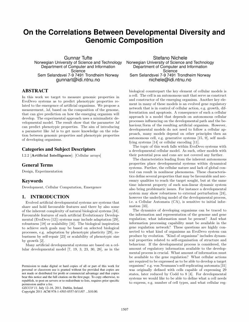
On the Correlations Between Developmental Diversity andGenomic Composition
Gunnar TufteNorwegian University of Science and Technology
Department of Computer and InformationScience
Sem Selandsvei 7-9 7491 Trondheim [email protected]
Stefano NicheleNorwegian University of Science and Technology
Department of Computer and InformationScience
Sem Selandsvei 7-9 7491 Trondheim [email protected]
ABSTRACTIn this work we target to measure genomic properties inEvoDevo systems as to predict phenotypic properties re-lated to the emergence of artificial organisms. We propose ameasurement, λd, based on the composition of the genome,that can give prediction on how the emerging organism willdevelop. The experimental approach uses a minimalistic de-velopmental model. The result show that the parameter λdcan predict phenotypic properties. The aim of introducinga parameter like λd is to get more knowledge on the rela-tion between genomic properties and phenotypic propertiesof developing organisms.
Categories and Subject DescriptorsI.2.2 [Artificial Intelligence]: [Cellular arrays]
General TermsDesign, Experimentation
KeywordsDevelopment, Cellular Computation, Emergence
1. INTRODUCTIONEvolved artificial developmental systems are systems that
share and hold favourable features and there by also someof the inherent complexity of natural biological systems [34].Favourable features of such artificial Evolutionary Develop-mental (EvoDevo [12]) systems may include adaptation [29],robustness [18] or scalability [16]. The biological inspirationto achieve such goals may be based on selected biologicalprocesses, e.g. adaptation by phenotypic plasticity [29], ro-bustness by self-repair [23] or scalability of phenotypic sizeby growth [2].
Many artificial developmental systems are based on a cel-lular developmental model [7, 19, 3, 23, 30, 28], as in the
Permission to make digital or hard copies of all or part of this work forpersonal or classroom use is granted without fee provided that copies arenot made or distributed for profit or commercial advantage and that copiesbear this notice and the full citation on the first page. To copy otherwise, torepublish, to post on servers or to redistribute to lists, requires prior specificpermission and/or a fee.GECCO’11, July 12–16, 2011, Dublin, Ireland.Copyright 2011 ACM 978-1-4503-0557-0/11/07 ...$10.00.
biological counterpart the key element of cellular models isa cell. The cell is an autonomous unit that serve as constructand constructor of the emerging organism. Another key ele-ment in many of these models is an evolved gene regulatorynetwork that is in control of cellular action, e.g. growth, dif-ferentiation and apoptosis. A consequence of such a cellularapproach is a model that depends on autonomous cellularprocesses influencing on the developmental path and the be-haviour/form of the resulting artificial organism. However,developmental models do not need to follow a cellular ap-proach, many models depend on other principles then anautonomous cell, e.g. generative systems [15, 9], self modi-fying systems [14] or cellular encoding [11].
The topic of this work falls within EvoDevo systems witha developmental cellular model. As such, other models withtheir potential pros and cons are not covered any further.
The characteristics leading from the inherent autonomousproperties place developmental systems within dynamicalsystems. Further, the cellular nature and lack of global con-trol can result in nonlinear phenomena. These characteris-tics define several properties that may be favourable and nec-essary qualities to reach the target sought, but at the sametime inherent property of such non-linear dynamic systemalso bring problematic issues. For instance a developmentalsystem may show robustness to external perturbation [24],however the underlying model of the developmental process,i.e. a Cellular Automata (CA), is sensitive to initial infor-mation [33].
The dynamics of developing organisms can be traced tothe information and representation of the genome and generegulation; what information must be present? And whatinformation processing capability must be available in thegene regulation network? These questions are highly con-nected to what kind of organisms an EvoDevo system canproduce by evolution. ”Kind of organisms” includes dynam-ical properties related to self-organisation of structure andbehaviour. If the developmental process is considered, theamount of regulatory information available to the develop-mental process is crucial. What amount of information mustbe available to the gene regulation? What cellular actionsare required to be expressed as to be able to develop a targetorganism? e.g. von Neumann’s self-replicating automata [31]was originally defined with cells capable of expressing 29states, later reduced by Codd to 8 [4]. For developmentalsystems we would like to be able to define what a cell needsto express, e.g. number of cell types, and what cellular reg-
1507
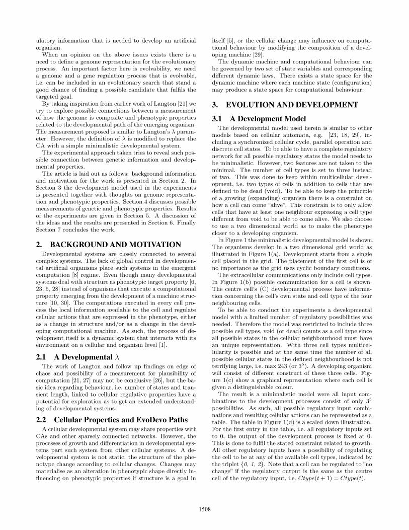
ulatory information that is needed to develop an artificialorganism.
When an opinion on the above issues exists there is aneed to define a genome representation for the evolutionaryprocess. An important factor here is evolvability, we needa genome and a gene regulation process that is evolvable,i.e. can be included in an evolutionary search that stand agood chance of finding a possible candidate that fulfils thetargeted goal.
By taking inspiration from earlier work of Langton [21] wetry to explore possible connections between a measurementof how the genome is composite and phenotypic propertiesrelated to the developmental path of the emerging organism.The measurement proposed is similar to Langton’s λ param-eter. However, the definition of λ is modified to replace theCA with a simple minimalistic developmental system.
The experimental approach taken tries to reveal such pos-sible connection between genetic information and develop-mental properties.
The article is laid out as follows: background informationand motivation for the work is presented in Section 2. InSection 3 the development model used in the experimentsis presented together with thoughts on genome representa-tion and phenotypic properties. Section 4 discusses possiblemeasurements of genetic and phenotypic properties. Resultsof the experiments are given in Section 5. A discussion ofthe ideas and the results are presented in Section 6. FinallySection 7 concludes the work.
2. BACKGROUND AND MOTIVATIONDevelopmental systems are closely connected to several
complex systems. The lack of global control in developmen-tal artificial organisms place such systems in the emergentcomputation [8] regime. Even though many developmentalsystems deal with structure as phenotypic target property [6,23, 5, 28] instead of organisms that execute a computationalproperty emerging from the development of a machine struc-ture [10, 30]. The computations executed in every cell pro-cess the local information available to the cell and regulatecellular actions that are expressed in the phenotype, eitheras a change in structure and/or as a change in the devel-oping computational machine. As such, the process of de-velopment itself is a dynamic system that interacts with itsenvironment on a cellular and organism level [1].
2.1 A Developmental λThe work of Langton and follow up findings on edge of
chaos and possibility of a measurement for plausibility ofcomputation [21, 27] may not be conclusive [26], but the ba-sic idea regarding behaviour, i.e. number of states and tran-sient length, linked to cellular regulative properties have apotential for exploration as to get an extended understand-ing of developmental systems.
2.2 Cellular Properties and EvoDevo PathsA cellular developmental system may share properties with
CAs and other sparsely connected networks. However, theprocesses of growth and differentiation in developmental sys-tems part such system from other cellular systems. A de-velopmental system is not static, the structure of the phe-notype change according to cellular changes. Changes maymaterialise as an alteration in phenotypic shape directly in-fluencing on phenotypic properties if structure is a goal in
itself [5], or the cellular change may influence on computa-tional behaviour by modifying the composition of a devel-oping machine [29].
The dynamic machine and computational behaviour canbe governed by two set of state variables and correspondingdifferent dynamic laws. There exists a state space for thedynamic machine where each machine state (configuration)may produce a state space for computational behaviour.
3. EVOLUTION AND DEVELOPMENT
3.1 A Development ModelThe developmental model used herein is similar to other
models based on cellular automata, e.g. [23, 18, 29], in-cluding a synchronized cellular cycle, parallel operation anddiscrete cell states. To be able to have a complete regulatorynetwork for all possible regulatory states the model needs tobe minimalistic. However, two features are not taken to theminimal. The number of cell types is set to three insteadof two. This was done to keep within multicellular devel-opment, i.e. two types of cells in addition to cells that aredefined to be dead (void). To be able to keep the principleof a growing (expanding) organism there is a constraint onhow a cell can come ”alive”. This constrain is to only allowcells that have at least one neighbour expressing a cell typedifferent from void to be able to come alive. We also chooseto use a two dimensional world as to make the phenotypecloser to a developing organism.
In Figure 1 the minimalistic developmental model is shown.The organisms develop in a two dimensional grid world asillustrated in Figure 1(a). Development starts from a singlecell placed in the grid. The placement of the first cell is ofno importance as the grid uses cyclic boundary conditions.
The extracellular communications only include cell types.In Figure 1(b) possible communication for a cell is shown.The centre cell’s (C) developmental process have informa-tion concerning the cell’s own state and cell type of the fourneighbouring cells.
To be able to conduct the experiments a developmentalmodel with a limited number of regulatory possibilities wasneeded. Therefore the model was restricted to include threepossible cell types, void (or dead) counts as a cell type sinceall possible states in the cellular neighbourhood must havean unique representation. With three cell types multicel-lularity is possible and at the same time the number of allpossible cellular states in the defined neighbourhood is notterrifying large, i.e. max 243 (or 35). A developing organismwill consist of different construct of these three cells. Fig-ure 1(c) show a graphical representation where each cell isgiven a distinguishable colour.
The result is a minimalistic model were all input com-binations to the development processes consist of only 35
possibilities. As such, all possible regulatory input combi-nations and resulting cellular actions can be represented as atable. The table in Figure 1(d) is a scaled down illustration.For the first entry in the table, i.e. all regulatory inputs setto 0, the output of the development process is fixed at 0.This is done to fulfil the stated constraint related to growth.All other regulatory inputs have a possibility of regulatingthe cell to be at any of the available cell types, indicated bythe triplet {0, 1, 2}. Note that a cell can be regulated to ”nochange” if the regulatory output is the same as the centrecell of the regulatory input, i.e. Ctype(t + 1) = Ctype(t).
1508
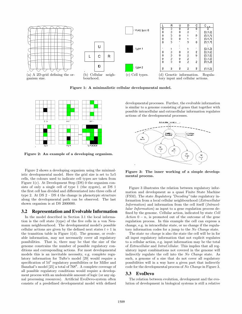
(a) A 2D-grid defining the or-ganism size.
(b) Cellular neigh-bourhood.
(c) Cell types. (d) Genetic information. Regula-tory input and cellular actions.
Figure 1: A minimalistic cellular developmental model.
Figure 2: An example of a developing organism.
Figure 2 shows a developing organism using the minimal-istic developmental model. Here the grid size is set to 5x5cells, the colours used to indicate cell types are taken fromFigure 1(c). At Development Step (DS) 0 the organism con-sists of only a single cell of type 1 (the zygote), at DS 1the first cell has divided and differentiated into three cells oftype 2. At DS 2 – DS 4 the change in phenotypic structurealong the developmental path can be observed. The lastshown organism is at DS 2000000.
3.2 Representation and Evolvable InformationIn the model described in Section 3.1 the local informa-
tion is the cell state (type) of the five cells in a von Neu-mann neighbourhood. The developmental model’s possiblecellular actions are given by the defined next states t + 1 inthe transition table in Figure 1(d). The genome, or evolv-able information, may not necessarily cover all regulatorypossibilities. That is, there may be that the size of thegenome constrains the number of possible regulatory con-ditions and corresponding actions. For most developmentalmodels this is an inevitable necessity, e.g. complete regu-latory information for Tufte’s model [29] would require aspecification of 545 regulatory possibilities or for Miller andBanzhaf’s model [25] a total of 7689. A complete coverage ofall possible regulatory conditions would require a develop-ment process with an undesirable amount of logic (or any sig-nal processing resources). Artificial EvoDevo-system oftenconsists of a predefined developmental model with defined
developmental processes. Further, the evolvable informationis similar to a genome consisting of genes that together withpossible intracellular and extracellular information regulatesactions of the developmental processes.
Figure 3: The inner working of a simple develop-mental process.
Figure 3 illustrates the relation between regulatory infor-mation and development as a quasi Finite State Machine(FSM). The state Regulatory ”Decoding” take regulatory in-formation from a local cellular neighbourhood (ExtracellularInformation) and information from the cell itself (Intracel-lular Information) as input to a gene regulation process de-fined by the genome. Cellular action, indicated by state CellAction 0 − n, is promoted out of the outcome of the generegulation process. In this example the cell can express achange, e.g. in intracellular state, or no change if the regula-tory information codes for a jump to the No Change state.
The state no change is also the state the cell will be in forall input regulatory information that not explicit regulatesto a cellular action, e.g. input information may be the totalof Extracellular and IntraCellular. This implies that all reg-ulatory input combinations not covered in the genome willindirectly regulate the cell into the No Change state. Assuch, a genome of a size that do not cover all regulatorypossibilities will in a way have a given part that indirectlycode for the developmental process of No Change in Figure 3.
3.3 EvoDevoThe relation between evolution, development and the evo-
lution of development in biological systems is still a relative
1509
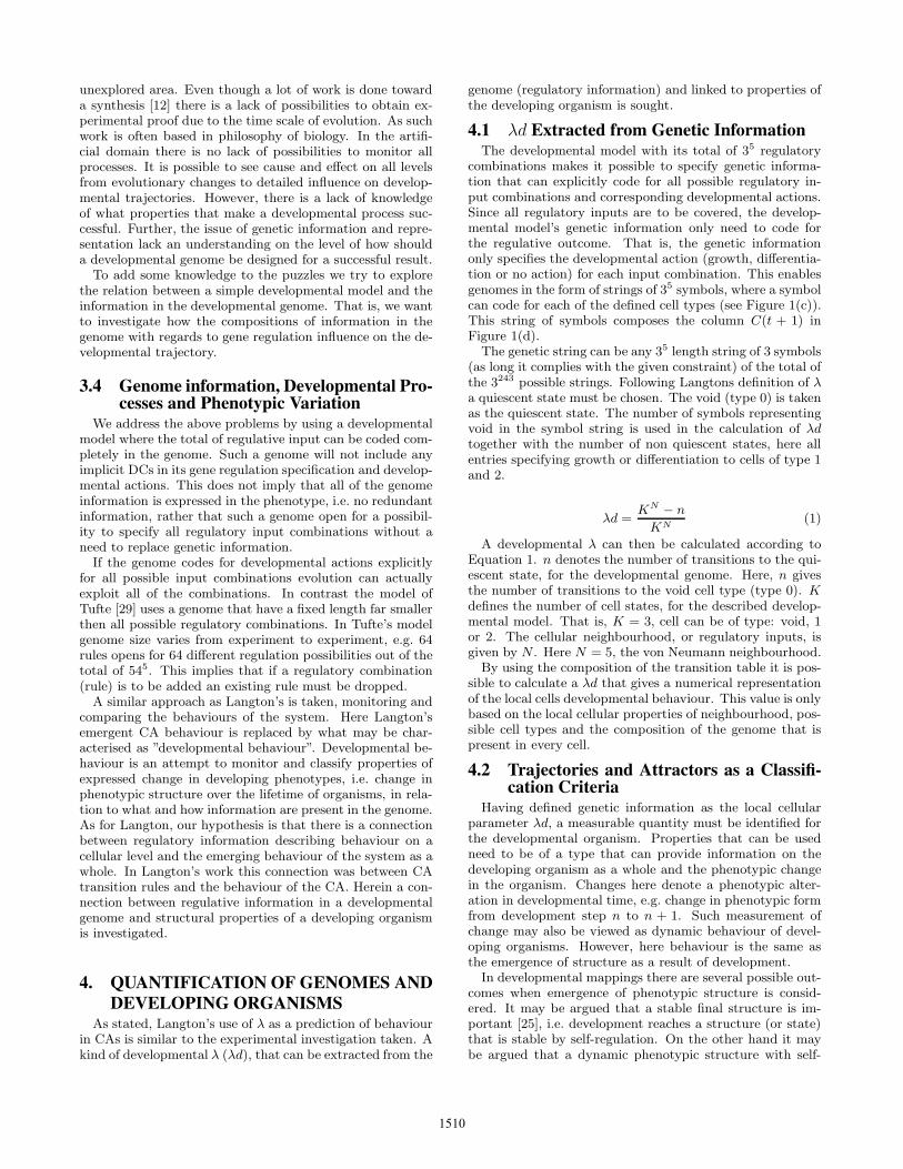
unexplored area. Even though a lot of work is done towarda synthesis [12] there is a lack of possibilities to obtain ex-perimental proof due to the time scale of evolution. As suchwork is often based in philosophy of biology. In the artifi-cial domain there is no lack of possibilities to monitor allprocesses. It is possible to see cause and effect on all levelsfrom evolutionary changes to detailed influence on develop-mental trajectories. However, there is a lack of knowledgeof what properties that make a developmental process suc-cessful. Further, the issue of genetic information and repre-sentation lack an understanding on the level of how shoulda developmental genome be designed for a successful result.
To add some knowledge to the puzzles we try to explorethe relation between a simple developmental model and theinformation in the developmental genome. That is, we wantto investigate how the compositions of information in thegenome with regards to gene regulation influence on the de-velopmental trajectory.
3.4 Genome information, Developmental Pro-cesses and Phenotypic Variation
We address the above problems by using a developmentalmodel where the total of regulative input can be coded com-pletely in the genome. Such a genome will not include anyimplicit DCs in its gene regulation specification and develop-mental actions. This does not imply that all of the genomeinformation is expressed in the phenotype, i.e. no redundantinformation, rather that such a genome open for a possibil-ity to specify all regulatory input combinations without aneed to replace genetic information.
If the genome codes for developmental actions explicitlyfor all possible input combinations evolution can actuallyexploit all of the combinations. In contrast the model ofTufte [29] uses a genome that have a fixed length far smallerthen all possible regulatory combinations. In Tufte’s modelgenome size varies from experiment to experiment, e.g. 64rules opens for 64 different regulation possibilities out of thetotal of 545. This implies that if a regulatory combination(rule) is to be added an existing rule must be dropped.
A similar approach as Langton’s is taken, monitoring andcomparing the behaviours of the system. Here Langton’semergent CA behaviour is replaced by what may be char-acterised as ”developmental behaviour”. Developmental be-haviour is an attempt to monitor and classify properties ofexpressed change in developing phenotypes, i.e. change inphenotypic structure over the lifetime of organisms, in rela-tion to what and how information are present in the genome.As for Langton, our hypothesis is that there is a connectionbetween regulatory information describing behaviour on acellular level and the emerging behaviour of the system as awhole. In Langton’s work this connection was between CAtransition rules and the behaviour of the CA. Herein a con-nection between regulative information in a developmentalgenome and structural properties of a developing organismis investigated.
4. QUANTIFICATION OF GENOMES ANDDEVELOPING ORGANISMS
As stated, Langton’s use of λ as a prediction of behaviourin CAs is similar to the experimental investigation taken. Akind of developmental λ (λd), that can be extracted from the
genome (regulatory information) and linked to properties ofthe developing organism is sought.
4.1 λd Extracted from Genetic InformationThe developmental model with its total of 35 regulatory
combinations makes it possible to specify genetic informa-tion that can explicitly code for all possible regulatory in-put combinations and corresponding developmental actions.Since all regulatory inputs are to be covered, the develop-mental model’s genetic information only need to code forthe regulative outcome. That is, the genetic informationonly specifies the developmental action (growth, differentia-tion or no action) for each input combination. This enablesgenomes in the form of strings of 35 symbols, where a symbolcan code for each of the defined cell types (see Figure 1(c)).This string of symbols composes the column C(t + 1) inFigure 1(d).
The genetic string can be any 35 length string of 3 symbols(as long it complies with the given constraint) of the total ofthe 3243 possible strings. Following Langtons definition of λa quiescent state must be chosen. The void (type 0) is takenas the quiescent state. The number of symbols representingvoid in the symbol string is used in the calculation of λdtogether with the number of non quiescent states, here allentries specifying growth or differentiation to cells of type 1and 2.
λd =KN − n
KN(1)
A developmental λ can then be calculated according toEquation 1. n denotes the number of transitions to the qui-escent state, for the developmental genome. Here, n givesthe number of transitions to the void cell type (type 0). Kdefines the number of cell states, for the described develop-mental model. That is, K = 3, cell can be of type: void, 1or 2. The cellular neighbourhood, or regulatory inputs, isgiven by N . Here N = 5, the von Neumann neighbourhood.
By using the composition of the transition table it is pos-sible to calculate a λd that gives a numerical representationof the local cells developmental behaviour. This value is onlybased on the local cellular properties of neighbourhood, pos-sible cell types and the composition of the genome that ispresent in every cell.
4.2 Trajectories and Attractors as a Classifi-cation Criteria
Having defined genetic information as the local cellularparameter λd, a measurable quantity must be identified forthe developmental organism. Properties that can be usedneed to be of a type that can provide information on thedeveloping organism as a whole and the phenotypic changein the organism. Changes here denote a phenotypic alter-ation in developmental time, e.g. change in phenotypic formfrom development step n to n + 1. Such measurement ofchange may also be viewed as dynamic behaviour of devel-oping organisms. However, here behaviour is the same asthe emergence of structure as a result of development.
In developmental mappings there are several possible out-comes when emergence of phenotypic structure is consid-ered. It may be argued that a stable final structure is im-portant [25], i.e. development reaches a structure (or state)that is stable by self-regulation. On the other hand it maybe argued that a dynamic phenotypic structure with self-
1510
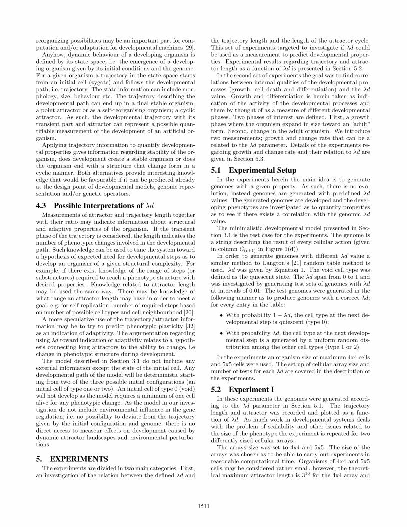
reorganizing possibilities may be an important part for com-putation and/or adaptation for developmental machines [29].
Anyhow, dynamic behaviour of a developing organism isdefined by its state space, i.e. the emergence of a develop-ing organism given by its initial conditions and the genome.For a given organism a trajectory in the state space startsfrom an initial cell (zygote) and follows the developmentalpath, i.e. trajectory. The state information can include mor-phology, size, behaviour etc. The trajectory describing thedevelopmental path can end up in a final stable organism;a point attractor or as a self-reorganising organism; a cyclicattractor. As such, the developmental trajectory with itstransient part and attractor can represent a possible quan-tifiable measurement of the development of an artificial or-ganism.
Applying trajectory information to quantify developmen-tal properties gives information regarding stability of the or-ganism, does development create a stable organism or doesthe organism end with a structure that change form in acyclic manner. Both alternatives provide interesting knowl-edge that would be favourable if it can be predicted alreadyat the design point of developmental models, genome repre-sentation and/or genetic operators.
4.3 Possible Interpretations of λdMeasurements of attractor and trajectory length together
with their ratio may indicate information about structuraland adaptive properties of the organism. If the transientphase of the trajectory is considered, the length indicates thenumber of phenotypic changes involved in the developmentalpath. Such knowledge can be used to tune the system towarda hypothesis of expected need for developmental steps as todevelop an organism of a given structural complexity. Forexample, if there exist knowledge of the range of steps (orsubstructures) required to reach a phenotype structure withdesired properties. Knowledge related to attractor lengthmay be used the same way. There may be knowledge ofwhat range an attractor length may have in order to meet agoal, e.g. for self-replication: number of required steps basedon number of possible cell types and cell neighbourhood [20].
A more speculative use of the trajectory/attractor infor-mation may be to try to predict phenotypic plasticity [32]as an indication of adaptivity. The argumentation regardingusing λd toward indication of adaptivity relates to a hypoth-esis connecting long attractors to the ability to change, i.echange in phenotypic structure during development.
The model described in Section 3.1 do not include anyexternal information except the state of the initial cell. Anydevelopmental path of the model will be deterministic start-ing from two of the three possible initial configurations (aninitial cell of type one or two). An initial cell of type 0 (void)will not develop as the model requires a minimum of one cellalive for any phenotypic change. As the model in our inves-tigation do not include environmental influence in the generegulation, i.e. no possibility to deviate from the trajectorygiven by the initial configuration and genome, there is nodirect access to measeur effects on development caused bydynamic attractor landscapes and environmental perturba-tions.
5. EXPERIMENTSThe experiments are divided in two main categories. First,
an investigation of the relation between the defined λd and
the trajectory length and the length of the attractor cycle.This set of experiments targeted to investigate if λd couldbe used as a measurement to predict developmental proper-ties. Experimental results regarding trajectory and attrac-tor length as a function of λd is presented in Section 5.2.
In the second set of experiments the goal was to find corre-lations between internal qualities of the developmental pro-cesses (growth, cell death and differentiation) and the λdvalue. Growth and differentiation is herein taken as indi-cation of the activity of the developmental processes andthere by thought of as a measure of different developmentalphases. Two phases of interest are defined. First, a growthphase where the organism expand in size toward an ”adult”form. Second, change in the adult organism. We introducetwo measurements; growth and change rate that can be arelated to the λd parameter. Details of the experiments re-garding growth and change rate and their relation to λd aregiven in Section 5.3.
5.1 Experimental SetupIn the experiments herein the main idea is to generate
genomes with a given property. As such, there is no evo-lution, instead genomes are generated with predefined λdvalues. The generated genomes are developed and the devel-oping phenotypes are investigated as to quantify propertiesas to see if there exists a correlation with the genomic λdvalue.
The minimalistic developmental model presented in Sec-tion 3.1 is the test case for the experiments. The genome isa string describing the result of every cellular action (givenin column C(t+1) in Figure 1(d)).
In order to generate genomes with different λd value asimilar method to Langton’s [21] random table method isused. λd was given by Equation 1. The void cell type wasdefined as the quiescent state. The λd span from 0 to 1 andwas investigated by generating test sets of genomes with λdat intervals of 0.01. The test genomes were generated in thefollowing manner as to produce genomes with a correct λd;for every entry in the table:
• With probability 1 − λd, the cell type at the next de-velopmental step is quiescent (type 0);
• With probability λd, the cell type at the next develop-mental step is a generated by a uniform random dis-tribution among the other cell types (type 1 or 2).
In the experiments an organism size of maximum 4x4 cellsand 5x5 cells were used. The set up of cellular array size andnumber of tests for each λd are covered in the description ofthe experiments.
5.2 Experiment IIn these experiments the genomes were generated accord-
ing to the λd parameter in Section 5.1. The trajectorylength and attractor was recorded and plotted as a func-tion of λd. As much work in developmental systems dealswith the problem of scalability and other issues related tothe size of the phenotype the experiment is repeated for twodifferently sized cellular arrays.
The arrays size was set to 4x4 and 5x5. The size of thearrays was chosen as to be able to carry out experiments inreasonable computational time. Organisms of 4x4 and 5x5cells may be considered rather small, however, the theoret-ical maximum attractor length is 316 for the 4x4 array and
1511
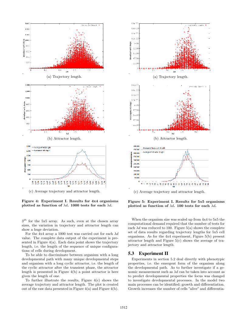
(a) Trajectory length.
(b) Attractor length.
(c) Average trajectory and attractor length.
Figure 4: Experiment I. Results for 4x4 organismsplotted as function of λd. 1000 tests for each λd.
325 for the 5x5 array. As such, even at the chosen arraysizes, the variation in trajectory and attractor length canshow a huge deviation.
For the 4x4 array a 1000 test was carried out for each λdvalue. The complete data output of the experiment is pre-sented in Figure 4(a). Each data point shows the trajectorylength, i.e. the length of the sequence of unique configura-tions of cells during development.
To be able to discriminate between organism with a longdevelopmental path with many unique developmental stepsand organism with a long cyclic attractor, i.e. the length ofthe cyclic attractor after the transient phase, the attractorlength is presented in Figure 4(b) a point attractor is heregiven the length of one.
To further illustrate the results, Figure 4(c) shows theaverage trajectory and attractor length. The plot is createdout of the raw data presented in Figure 4(a) and Figure 4(b).
(a) Trajectory length.
(b) Attractor length.
(c) Average trajectory and attractor length.
Figure 5: Experiment I. Results for 5x5 organismsplotted as function of λd. 100 tests for each λd.
When the organism size was scaled up from 4x4 to 5x5 thecomputational demand required that the number of tests foreach λd was reduced to 100. Figure 5(a) shows the completeset of data results regarding trajectory lengths for 5x5 cellorganisms. As for the 4x4 experiment, Figure 5(b) presentattractor length and Figure 5(c) shows the average of tra-jectory and attractor length.
5.3 Experiment IIExperiments in section 5.2 deal directly with phenotypic
properties, i.e. the emergent form of the organism alongthe developmental path. As to further investigate if a ge-nomic measurement such as λd can be taken into account asto predict developmental properties the focus was changedto investigate developmental processes. In the model twomain processes can be identified; growth and differentiation.Growth increases the number of cells ”alive” and differentia-
1512
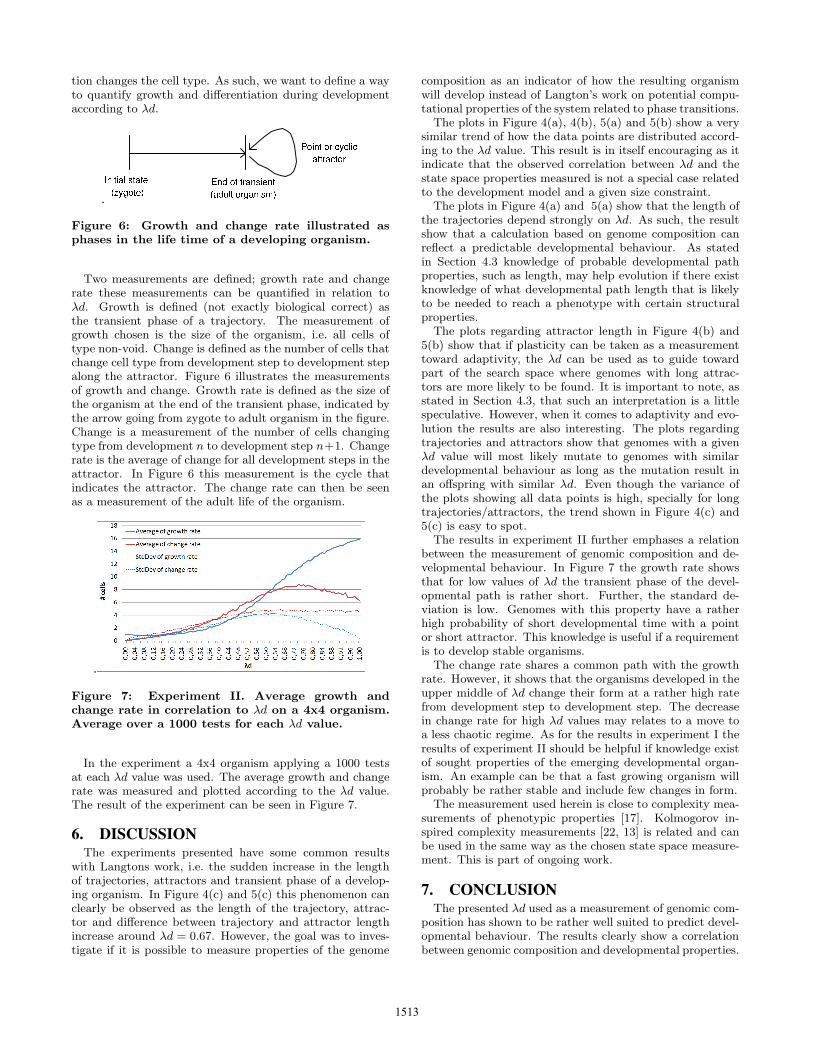
tion changes the cell type. As such, we want to define a wayto quantify growth and differentiation during developmentaccording to λd.
Figure 6: Growth and change rate illustrated asphases in the life time of a developing organism.
Two measurements are defined; growth rate and changerate these measurements can be quantified in relation toλd. Growth is defined (not exactly biological correct) asthe transient phase of a trajectory. The measurement ofgrowth chosen is the size of the organism, i.e. all cells oftype non-void. Change is defined as the number of cells thatchange cell type from development step to development stepalong the attractor. Figure 6 illustrates the measurementsof growth and change. Growth rate is defined as the size ofthe organism at the end of the transient phase, indicated bythe arrow going from zygote to adult organism in the figure.Change is a measurement of the number of cells changingtype from development n to development step n+1. Changerate is the average of change for all development steps in theattractor. In Figure 6 this measurement is the cycle thatindicates the attractor. The change rate can then be seenas a measurement of the adult life of the organism.
Figure 7: Experiment II. Average growth andchange rate in correlation to λd on a 4x4 organism.Average over a 1000 tests for each λd value.
In the experiment a 4x4 organism applying a 1000 testsat each λd value was used. The average growth and changerate was measured and plotted according to the λd value.The result of the experiment can be seen in Figure 7.
6. DISCUSSIONThe experiments presented have some common results
with Langtons work, i.e. the sudden increase in the lengthof trajectories, attractors and transient phase of a develop-ing organism. In Figure 4(c) and 5(c) this phenomenon canclearly be observed as the length of the trajectory, attrac-tor and difference between trajectory and attractor lengthincrease around λd = 0.67. However, the goal was to inves-tigate if it is possible to measure properties of the genome
composition as an indicator of how the resulting organismwill develop instead of Langton’s work on potential compu-tational properties of the system related to phase transitions.
The plots in Figure 4(a), 4(b), 5(a) and 5(b) show a verysimilar trend of how the data points are distributed accord-ing to the λd value. This result is in itself encouraging as itindicate that the observed correlation between λd and thestate space properties measured is not a special case relatedto the development model and a given size constraint.
The plots in Figure 4(a) and 5(a) show that the length ofthe trajectories depend strongly on λd. As such, the resultshow that a calculation based on genome composition canreflect a predictable developmental behaviour. As statedin Section 4.3 knowledge of probable developmental pathproperties, such as length, may help evolution if there existknowledge of what developmental path length that is likelyto be needed to reach a phenotype with certain structuralproperties.
The plots regarding attractor length in Figure 4(b) and5(b) show that if plasticity can be taken as a measurementtoward adaptivity, the λd can be used as to guide towardpart of the search space where genomes with long attrac-tors are more likely to be found. It is important to note, asstated in Section 4.3, that such an interpretation is a littlespeculative. However, when it comes to adaptivity and evo-lution the results are also interesting. The plots regardingtrajectories and attractors show that genomes with a givenλd value will most likely mutate to genomes with similardevelopmental behaviour as long as the mutation result inan offspring with similar λd. Even though the variance ofthe plots showing all data points is high, specially for longtrajectories/attractors, the trend shown in Figure 4(c) and5(c) is easy to spot.
The results in experiment II further emphases a relationbetween the measurement of genomic composition and de-velopmental behaviour. In Figure 7 the growth rate showsthat for low values of λd the transient phase of the devel-opmental path is rather short. Further, the standard de-viation is low. Genomes with this property have a ratherhigh probability of short developmental time with a pointor short attractor. This knowledge is useful if a requirementis to develop stable organisms.
The change rate shares a common path with the growthrate. However, it shows that the organisms developed in theupper middle of λd change their form at a rather high ratefrom development step to development step. The decreasein change rate for high λd values may relates to a move toa less chaotic regime. As for the results in experiment I theresults of experiment II should be helpful if knowledge existof sought properties of the emerging developmental organ-ism. An example can be that a fast growing organism willprobably be rather stable and include few changes in form.
The measurement used herein is close to complexity mea-surements of phenotypic properties [17]. Kolmogorov in-spired complexity measurements [22, 13] is related and canbe used in the same way as the chosen state space measure-ment. This is part of ongoing work.
7. CONCLUSIONThe presented λd used as a measurement of genomic com-
position has shown to be rather well suited to predict devel-opmental behaviour. The results clearly show a correlationbetween genomic composition and developmental properties.
1513
The distribution of developmental behaviour according toλd found can be exploited as to be able to design EvoDevosystems with smoother search space. Further, if there existknowledge of developmental properties related to the de-velopment of form, parameters like λd can be exploited topoint evolution toward parts of the search space where theexistence of sought behaviour is more likely. Another im-portant use of parameters, such as λd, is in the design phaseof EvoDevo systems. If the system is not able to exhibitbehaviour in the different regimes resulting from differentλd values, it is given that the system can not be appliedto problems that most likely require such developmental be-haviour.
8. REFERENCES[1] R. D. Beer. A dynamical systems perspective on
agent-environment interaction. Artificial Intelligence,1–2(72):173–215, 1995.
[2] P. J. Bentley and S. Kumar. Three ways to grow designs: Acomparison of embryogenies for an evolutionary designproblem. In Genetic and Evolutionary ComputationConference (GECCO ’99), pages 35–43, 1999.
[3] J. C. Bongard and R. Pfeifer. Morpho-functional Machines:The New Species (Designing Embodied Intelligence),chapter Evolving complete agents using artificial ontogeny,pages 237–258. Springer-Verlag, 2003.
[4] E. F. Codd. Cellular Automata. Association for computingmachinery, Inc. Monograph series. Academic Press, NewYork, 1968.
[5] S. Cussat-Blanc, H. Luga, and Y. Duthen. From single cellto simple creature morphology and metabolism. InS. Bullock, J. Noble, R. Watson, and M. A. Bedau, editors,Artificial Life XI: Proceedings of the Eleventh InternationalConference on the Simulation and Synthesis of LivingSystems, pages 134–141. MIT Press, Cambridge, MA, 2008.
[6] P. Eggenberger. Evolving morphologies of simulated 3dorganisms based on differential gene expression. In FourthEuropean Conference on Artificial Life, pages 205–213.MIT press, 1997.
[7] K. Fleischer and A. H. Barr. A simulation testbed for thestudy of multicellular development: The multiplemechanisms of morphogenesis. In Artificial Life III, pages389–416. Addison-Wesley, 1993.
[8] S. Forrest. Emergent Computation. MIT Press, 1991.[9] J. Gauci and K. Stanley. Generating large-scale neural
networks through discovering geometric regularities. InGECCO ’07: Proceedings of the 9th annual conference onGenetic and evolutionary computation, pages 997–1004,New York, NY, USA, 2007. ACM.
[10] T. G. W. Gordon. Exploring models of development forevolutionary circuit design. In 2003 Congress onEvolutionary Computation (CEC 2003), pages 2050–2057.IEEE, 2003.
[11] F. Gruau. Cellular encoding of genetic neural networks.Technical report 92-21, Laboratoire de l’Informatique duParallilisme. Ecole Normale Supirieure de Lyon, France,1992.
[12] B. K. Hall, R. D. Pearson, and G. B. Muller. Environment,development, and Evolution Toward a Synthesis. TheVienna Series in Theoretical Biology. MIT-Press, 2004.
[13] S. Harding and W. Banzhaf. Organic Computing, chapterArtificial Development, pages 201 – 220. Springer Verlag,2008.
[14] S. L. Harding, J. F. Miller, and W. Banzhaf. Self-modifyingcartesian genetic programming. In GECCO ’07:Proceedings of the 9th annual conference on Genetic andevolutionary computation, pages 1021–1028, New York,NY, USA, 2007. ACM.
[15] G. S. Hornby and J. B. Pollack. The advantages ofgenerative grammatical encodings for physical design. In
Congress on Evolutionary Computation (CEC 2001).IEEE, 2001.
[16] H. Kitano. Building complex systems using developmentprocess: An engineering approach. In Evolvable Systems:from Biology to Hardware, ICES, Lecture Notes inComputer Science, pages 218–229. Springer, 1998.
[17] T. Kowaliw. Measures of complexity for artificialembryogeny. In GECCO ’08: Proceedings of the 10thannual conference on Genetic and EvolutionaryComputation. ACM, 2008.
[18] T. Kowaliw, P. Grogono, and N. Kharma. Environment asa spatial constraint on the growth of structural form. InGECCO ’07: Proceedings of the 9th annual conference onGenetic and evolutionary computation, pages 1037–1044,New York, NY, USA, 2007. ACM.
[19] S. Kumar and P. J. Bentley. Biologically inspiredevolutionary development. In 5th International Conferenceon Evolvable Systems (ICES03), Lecture Notes inComputer Science, pages 57–68. Springer, 2003.
[20] C. G. Langton. Self-reproduction in cellular automata.Physica D, 10:135–144, 1984.
[21] C. G. Langton. Computation at the edge of chaos: phasetransitions and emergant computation. In S. Forrest, editor,Emergent Computation, pages 12–37. MIT Press, 1991.
[22] P. K. Lehre and P. C. Haddow. Developmental mappingsand phenotypic complexity. In Congress on EvolutionaryComputation(CEC2003), pages 62–68. IEEE, 2003.
[23] J. F. Miller. Evolving developmental programs foradaptation, morphogenesis, and self-repair. In SeventhEuropean Conference on Artificial Life, Lecture Notes inArtificial Intelligence, pages 256–265. Springer, 2003.
[24] J. F. Miller. Evolving a self-repairing, self-regulating, frenchflag organism. In Genetic and Evolutionary Computation(GECCO 2004), Lecture Notes in Computer Science, pages129–139. Springer, 2004.
[25] J. F. Miller and W. Banzhaf. Evolving the program for acell: from french flag to boolean circuits. In S. Kumar andP. J. Bentley, editors, On Growth, Form and Computers,pages 278–301. Elsevier Limited Oxford UK, 2003.
[26] M. Mitchell, P. T. Hraber, and J. P. Crutchfield. revisitingthe egde of chaos: Evolving cellular automata to performcomputations. Complex Systems, 7:89–130, 1993. Santa FeInstitute Working Paper 93-03-014.
[27] N. H. Packard. Dynamic Patterns in Complex Systems,chapter Adaptation Toward the Edge of Chaos, pages293–301. World Scientific, 1988.
[28] T. Steiner, Y. Jin, and B. Sendhoff. A cellular model forthe evolutionary development of lightweight material withan inner structure. In GECCO ’08: Proceedings of the 10thannual conference on Genetic and evolutionarycomputation, pages 851–858, New York, NY, USA, 2008.ACM.
[29] G. Tufte. Evolution, development and environment towardadaptation through phenotypic plasticity and exploitationof external information. In S. Bullock, J. Noble, R. Watson,and M. A. Bedau, editors, Artificial Life XI: Proceedings ofthe Eleventh International Conference on the Simulationand Synthesis of Living Systems, pages 624–631. MITPress, Cambridge, MA, 2008.
[30] G. Tufte and P. C. Haddow. Towards development on asilicon-based cellular computation machine. NaturalComputation, 4(4):387–416, 2005.
[31] J. von Neumann. Theory of Self-Reproducing Automata.University of Illinois Press, Urbana, IL, USA, 1966., 1966.
[32] M. J. West-Eberhard. Developmental Plasticity andEvolution. Oxford University Press, 2003.
[33] S. Wolfram. Universality and complexity in cellularautomata. Physica D, 10(1-2):1–35, 1984.
[34] L. Wolpert. Principles of Development, Second edition.Oxford University Press, 2002.
1514
Paper A.2
Genome Parameters as Information to Forecast
Emergent Developmental Behaviors
S. Nichele and G. Tufte
11th International Conference on Unconventional Computation and Natural
Computation, UCNC 2012
September 3 - 7, 2012
Orleans, France

60
J. Durand-Lose and N. Jonoska (Eds.): UCNC 2012, LNCS 7445, pp. 186–197, 2012. © Springer-Verlag Berlin Heidelberg 2012
Genome Parameters as Information to Forecast Emergent Developmental Behaviors
Stefano Nichele and Gunnar Tufte
Norwegian University of Science and Technology, Department of Computer and Information Science,
Sem Selandsvei 7-9, 7491, Trondheim, Norway {nichele,gunnart}@idi.ntnu.no
Abstract. In this paper we measure genomic properties in EvoDevo systems, to predict emergent phenotypic characteristic of artificial organisms. We describe and compare three parameters calculated out of the composition of the genome, to forecast the emergent behavior and structural properties of the developed or-ganisms. The parameters are each calculated by including different genomic in-formation. The genotypic information explored are: purely regulatory output, regulatory input and relative output considered independently and an overall pa-rameter calculated out of genetic dependency properties. The goal of this work is to gain more knowledge on the relation between genotypes and the behavior of emergent phenotypes. Such knowledge will give information on genetic composition in relation to artificial developmental organisms, providing guide-lines for construction of EvoDevo systems. A minimalistic developmental sys-tem based on Cellular Automata is chosen in the experimental work.
Keywords: Development, Cellular Computation, Emergence, Evolution, Para-meterization of Rule Spaces.
1 Introduction
Artificial developmental systems are systems that can be used to grow artificial or-ganisms, exploiting an indirect genotype to phenotype mapping [9]. Indirect mapping between genotype and phenotype enables two organisms with identical genes to de-velop to diverting phenotypes, caused by factors influencing the development process, e.g. interactions with the environment. Several artificial developmental systems take inspiration from cellular models [12, 19, 24, 27], where the key element is a cell. The way a cell behaves can be represented by gene regulation that encapsulates the rules and actions that a cell may perform, e.g. growth, differentiation, death. The result of such architecture is a system that can show different developmental behaviors from a single cell (zygote) to a multi-cellular organism.
Even if an artificial developmental process itself can be regulated by very simple mechanisms at cellular level, the whole emergent behavior of the system can show complex phenotypes with properties of stability or unpredictable self-reorganization.
Genome Parameters as Information to Forecast Emergent Developmental Behaviors 187
Evolutionary Developmental (EvoDevo) systems [15] have been used in a wide varie-ty of experiments with promising results (e.g. to reach a phenotypic target property [24], to execute a computational property emerging from the development of a ma-chine structure [27] or to develop modular structures [9]), but at the theoretical level the amount of knowledge is limited. This work is focused on the underlying proper-ties of EvoDevo systems and thus does not aim to develop specific organisms with specific properties. Rather, we want to gain more knowledge on the dynamics of de-veloping organisms in relation with the information and representation of the genome and gene regulation.
In this work, the genotypes are represented as a transition rule table, where deve-lopmental actions are defined as function of the neighborhood configuration. In this way, it is possible to analyze the different developmental actions and calculate para-meters obtained from the genome table. We investigate three different genome para-meters. The first one takes inspiration from earlier work of Langton [21], using a developmental λ which is based only on the output of the genomic developmental table. The second parameter is the Majority parameter, a measure of regulatory input and relative output considered independently. This approach is similar to Neighbor-hood Dominance parameter described in [4]. The third is the Sensitivity parameter, an overall measure of the developmental table where table entries are dependent one to another, defined by Binder [1, 2]. Every parameter measures a different feature of the genome information and thus should be able to describe different phenotypic behaviors.
The article is laid out as follows: background information and motivation for the work is given in Section 2. In Section 3 the developmental model used in the experi-ments is described. Section 4 presents the used parameters in details. Section 5 shows the results of the experiments. The discussion of the results is given in Section 6 to-gether with the conclusions.
2 Background and Motivation
Artificial developmental systems fall within the field of complex systems. In complex systems, the focus is on the global behavior rather than on the local behavior of the single parts from which the system is built. The interwoven interaction of the system components, without the action of a global controller, places such systems in the field of emergent computation [13].
A CA can be considered as a developing organism, where the genome specifica-tions and the gene regulation information control the cells’ growth and differentiation. The behavior of the CA is represented by the emergent phenotype, which is subject to size and shape modifications, according to the cellular changes along the develop-mental process. Such dynamic developmental systems can show adaptation, self-modification, plasticity [28] or self-replication [20] properties.
The works of Wolfram [29] and Langton [21] on the computation of cellular ma-chines laid a foundation for further research on the possibility of “measuring” properties of the computation [26] and develop a better understanding of the emergent behavior of
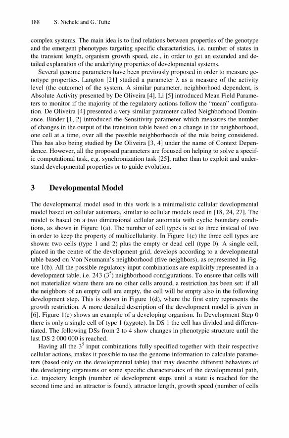
188 S. Nichele and G. Tufte
complex systems. The main idea is to find relations between properties of the genotype and the emergent phenotypes targeting specific characteristics, i.e. number of states in the transient length, organism growth speed, etc., in order to get an extended and de-tailed explanation of the underlying properties of developmental systems.
Several genome parameters have been previously proposed in order to measure ge-notype properties. Langton [21] studied a parameter λ as a measure of the activity level (the outcome) of the system. A similar parameter, neighborhood dependent, is Absolute Activity presented by De Oliveira [4]. Li [5] introduced Mean Field Parame-ters to monitor if the majority of the regulatory actions follow the “mean” configura-tion. De Oliveira [4] presented a very similar parameter called Neighborhood Domin-ance. Binder [1, 2] introduced the Sensitivity parameter which measures the number of changes in the output of the transition table based on a change in the neighborhood, one cell at a time, over all the possible neighborhoods of the rule being considered. This has also being studied by De Oliveira [3, 4] under the name of Context Depen-dence. However, all the proposed parameters are focused on helping to solve a specif-ic computational task, e.g. synchronization task [25], rather than to exploit and under-stand developmental properties or to guide evolution.
3 Developmental Model
The developmental model used in this work is a minimalistic cellular developmental model based on cellular automata, similar to cellular models used in [18, 24, 27]. The model is based on a two dimensional cellular automata with cyclic boundary condi-tions, as shown in Figure 1(a). The number of cell types is set to three instead of two in order to keep the property of multicellularity. In Figure 1(c) the three cell types are shown: two cells (type 1 and 2) plus the empty or dead cell (type 0). A single cell, placed in the centre of the development grid, develops according to a developmental table based on Von Neumann’s neighborhood (five neighbors), as represented in Fig-ure 1(b). All the possible regulatory input combinations are explicitly represented in a development table, i.e. 243 (35) neighborhood configurations. To ensure that cells will not materialize where there are no other cells around, a restriction has been set: if all the neighbors of an empty cell are empty, the cell will be empty also in the following development step. This is shown in Figure 1(d), where the first entry represents the growth restriction. A more detailed description of the development model is given in [6]. Figure 1(e) shows an example of a developing organism. In Development Step 0 there is only a single cell of type 1 (zygote). In DS 1 the cell has divided and differen-tiated. The following DSs from 2 to 4 show changes in phenotypic structure until the last DS 2 000 000 is reached.
Having all the 35 input combinations fully specified together with their respective cellular actions, makes it possible to use the genome information to calculate parame-ters (based only on the developmental table) that may describe different behaviors of the developing organisms or some specific characteristics of the developmental path, i.e. trajectory length (number of development steps until a state is reached for the second time and an attractor is found), attractor length, growth speed (number of cells
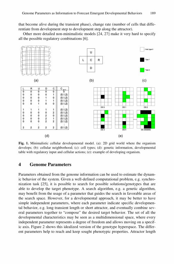
Genome Parameters as Information to Forecast Emergent Developmental Behaviors 189
that become alive during the transient phase), change rate (number of cells that diffe-rentiate from development step to development step along the attractor).
Other more detailed non-minimalistic models [24, 27] make it very hard to specify all the possible regulatory combinations [6].
Fig. 1. Minimalistic cellular developmental model. (a): 2D grid world where the organism develops; (b): cellular neighborhood; (c): cell types; (d): genetic information, developmental table with regulatory input and cellular actions; (e): example of developing organism.
4 Genome Parameters
Parameters obtained from the genome information can be used to estimate the dynam-ic behavior of the system. Given a well-defined computational problem, e.g. synchro-nization task [25], it is possible to search for possible solutions/genotypes that are able to develop the target phenotype. A search algorithm, e.g. a genetic algorithm, may benefit from the usage of a parameter that guides the search in favorable areas of the search space. However, for a developmental approach, it may be better to have simple independent parameters, where each parameter indicate specific developmen-tal behavior, e.g. long transient length or short attractor, and eventually combine sev-eral parameters together to “compose” the desired target behavior. The set of all the developmental characteristics may be seen as a multidimensional space, where every independent parameter represents a degree of freedom and allows moving on a specif-ic axis. Figure 2 shows this idealized version of the genotype hyperspace. The differ-ent parameters help to reach and keep sought phenotypic properties. Attractor length
(a) (b) (c)
(d) (e)
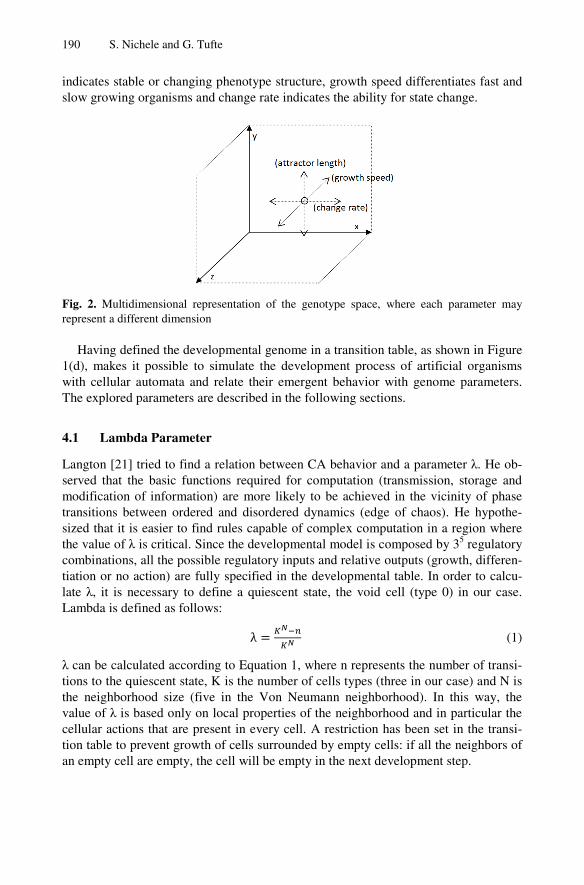
190 S. Nichele and G. Tufte
indicates stable or changing phenotype structure, growth speed differentiates fast and slow growing organisms and change rate indicates the ability for state change.
Fig. 2. Multidimensional representation of the genotype space, where each parameter may represent a different dimension
Having defined the developmental genome in a transition table, as shown in Figure 1(d), makes it possible to simulate the development process of artificial organisms with cellular automata and relate their emergent behavior with genome parameters. The explored parameters are described in the following sections.
4.1 Lambda Parameter
Langton [21] tried to find a relation between CA behavior and a parameter λ. He ob-served that the basic functions required for computation (transmission, storage and modification of information) are more likely to be achieved in the vicinity of phase transitions between ordered and disordered dynamics (edge of chaos). He hypothe-sized that it is easier to find rules capable of complex computation in a region where the value of λ is critical. Since the developmental model is composed by 35 regulatory combinations, all the possible regulatory inputs and relative outputs (growth, differen-tiation or no action) are fully specified in the developmental table. In order to calcu-late λ, it is necessary to define a quiescent state, the void cell (type 0) in our case. Lambda is defined as follows: λ (1)
λ can be calculated according to Equation 1, where n represents the number of transi-tions to the quiescent state, K is the number of cells types (three in our case) and N is the neighborhood size (five in the Von Neumann neighborhood). In this way, the value of λ is based only on local properties of the neighborhood and in particular the cellular actions that are present in every cell. A restriction has been set in the transi-tion table to prevent growth of cells surrounded by empty cells: if all the neighbors of an empty cell are empty, the cell will be empty in the next development step.
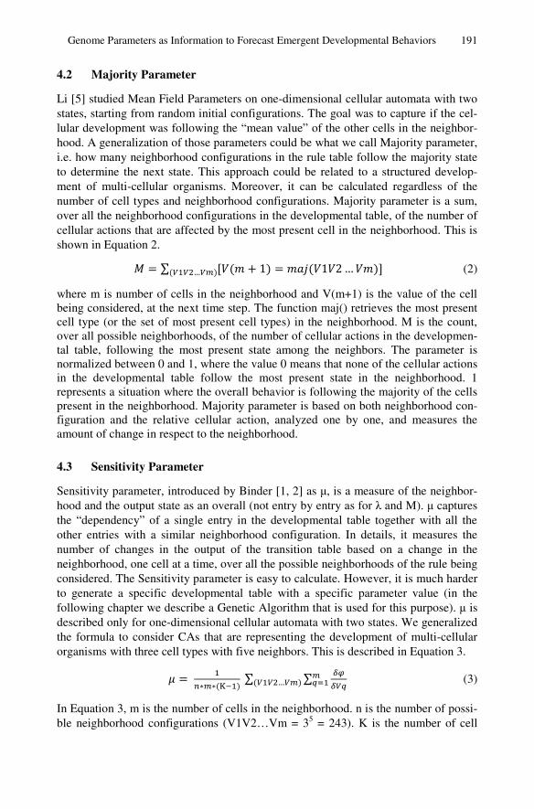
Genome Parameters as Information to Forecast Emergent Developmental Behaviors 191
4.2 Majority Parameter
Li [5] studied Mean Field Parameters on one-dimensional cellular automata with two states, starting from random initial configurations. The goal was to capture if the cel-lular development was following the “mean value” of the other cells in the neighbor-hood. A generalization of those parameters could be what we call Majority parameter, i.e. how many neighborhood configurations in the rule table follow the majority state to determine the next state. This approach could be related to a structured develop-ment of multi-cellular organisms. Moreover, it can be calculated regardless of the number of cell types and neighborhood configurations. Majority parameter is a sum, over all the neighborhood configurations in the developmental table, of the number of cellular actions that are affected by the most present cell in the neighborhood. This is shown in Equation 2. ∑ 1 1 2 …… (2)
where m is number of cells in the neighborhood and V(m+1) is the value of the cell being considered, at the next time step. The function maj() retrieves the most present cell type (or the set of most present cell types) in the neighborhood. M is the count, over all possible neighborhoods, of the number of cellular actions in the developmen-tal table, following the most present state among the neighbors. The parameter is normalized between 0 and 1, where the value 0 means that none of the cellular actions in the developmental table follow the most present state in the neighborhood. 1 represents a situation where the overall behavior is following the majority of the cells present in the neighborhood. Majority parameter is based on both neighborhood con-figuration and the relative cellular action, analyzed one by one, and measures the amount of change in respect to the neighborhood.
4.3 Sensitivity Parameter
Sensitivity parameter, introduced by Binder [1, 2] as μ, is a measure of the neighbor-hood and the output state as an overall (not entry by entry as for λ and M). μ captures the “dependency” of a single entry in the developmental table together with all the other entries with a similar neighborhood configuration. In details, it measures the number of changes in the output of the transition table based on a change in the neighborhood, one cell at a time, over all the possible neighborhoods of the rule being considered. The Sensitivity parameter is easy to calculate. However, it is much harder to generate a specific developmental table with a specific parameter value (in the following chapter we describe a Genetic Algorithm that is used for this purpose). μ is described only for one-dimensional cellular automata with two states. We generalized the formula to consider CAs that are representing the development of multi-cellular organisms with three cell types with five neighbors. This is described in Equation 3. K ∑ ∑… (3)
In Equation 3, m is the number of cells in the neighborhood. n is the number of possi-ble neighborhood configurations (V1V2…Vm = 35 = 243). K is the number of cell
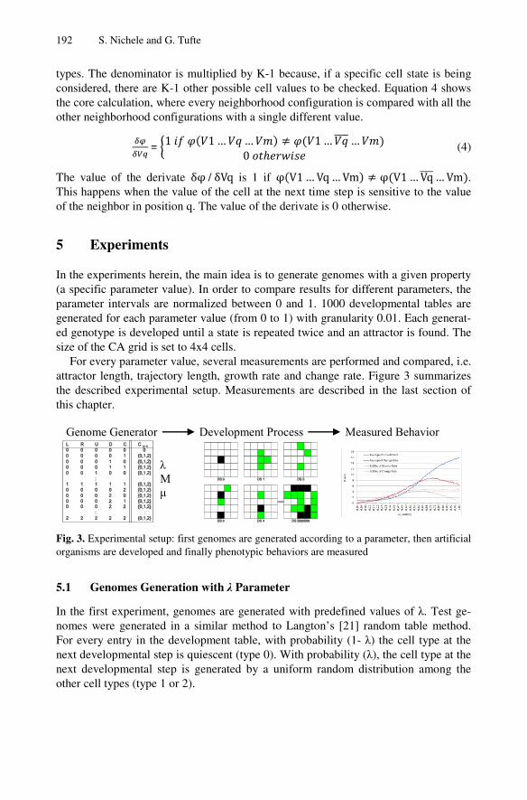
192 S. Nichele and G. Tufte
types. The denominator is multiplied by K-1 because, if a specific cell state is being considered, there are K-1 other possible cell values to be checked. Equation 4 shows the core calculation, where every neighborhood configuration is compared with all the other neighborhood configurations with a single different value. = 1 1 … … 1 … …0 (4)
The value of the derivate δφ / δVq is 1 if φ V1 … Vq … Vm φ V1 … Vq … Vm . This happens when the value of the cell at the next time step is sensitive to the value of the neighbor in position q. The value of the derivate is 0 otherwise.
5 Experiments
In the experiments herein, the main idea is to generate genomes with a given property (a specific parameter value). In order to compare results for different parameters, the parameter intervals are normalized between 0 and 1. 1000 developmental tables are generated for each parameter value (from 0 to 1) with granularity 0.01. Each generat-ed genotype is developed until a state is repeated twice and an attractor is found. The size of the CA grid is set to 4x4 cells.
For every parameter value, several measurements are performed and compared, i.e. attractor length, trajectory length, growth rate and change rate. Figure 3 summarizes the described experimental setup. Measurements are described in the last section of this chapter.
Fig. 3. Experimental setup: first genomes are generated according to a parameter, then artificial organisms are developed and finally phenotypic behaviors are measured
5.1 Genomes Generation with λ Parameter
In the first experiment, genomes are generated with predefined values of λ. Test ge-nomes were generated in a similar method to Langton’s [21] random table method. For every entry in the development table, with probability (1- λ) the cell type at the next developmental step is quiescent (type 0). With probability (λ), the cell type at the next developmental step is generated by a uniform random distribution among the other cell types (type 1 or 2).
Genome Generator Development Process Measured Behavior
λ M μ
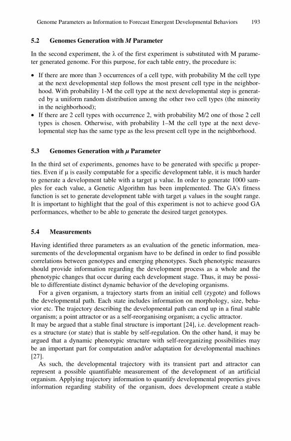
Genome Parameters as Information to Forecast Emergent Developmental Behaviors 193
5.2 Genomes Generation with M Parameter
In the second experiment, the λ of the first experiment is substituted with M parame-ter generated genome. For this purpose, for each table entry, the procedure is:
• If there are more than 3 occurrences of a cell type, with probability M the cell type at the next developmental step follows the most present cell type in the neighbor-hood. With probability 1-M the cell type at the next developmental step is generat-ed by a uniform random distribution among the other two cell types (the minority in the neighborhood);
• If there are 2 cell types with occurrence 2, with probability M/2 one of those 2 cell types is chosen. Otherwise, with probability 1–M the cell type at the next deve-lopmental step has the same type as the less present cell type in the neighborhood.
5.3 Genomes Generation with μ Parameter
In the third set of experiments, genomes have to be generated with specific μ proper-ties. Even if μ is easily computable for a specific development table, it is much harder to generate a development table with a target μ value. In order to generate 1000 sam-ples for each value, a Genetic Algorithm has been implemented. The GA's fitness function is set to generate development table with target μ values in the sought range. It is important to highlight that the goal of this experiment is not to achieve good GA performances, whether to be able to generate the desired target genotypes.
5.4 Measurements
Having identified three parameters as an evaluation of the genetic information, mea-surements of the developmental organism have to be defined in order to find possible correlations between genotypes and emerging phenotypes. Such phenotypic measures should provide information regarding the development process as a whole and the phenotypic changes that occur during each development stage. Thus, it may be possi-ble to differentiate distinct dynamic behavior of the developing organisms.
For a given organism, a trajectory starts from an initial cell (zygote) and follows the developmental path. Each state includes information on morphology, size, beha-vior etc. The trajectory describing the developmental path can end up in a final stable organism; a point attractor or as a self-reorganising organism; a cyclic attractor. It may be argued that a stable final structure is important [24], i.e. development reach-es a structure (or state) that is stable by self-regulation. On the other hand, it may be argued that a dynamic phenotypic structure with self-reorganizing possibilities may be an important part for computation and/or adaptation for developmental machines [27].
As such, the developmental trajectory with its transient part and attractor can represent a possible quantifiable measurement of the development of an artificial organism. Applying trajectory information to quantify developmental properties gives information regarding stability of the organism, does development create a stable
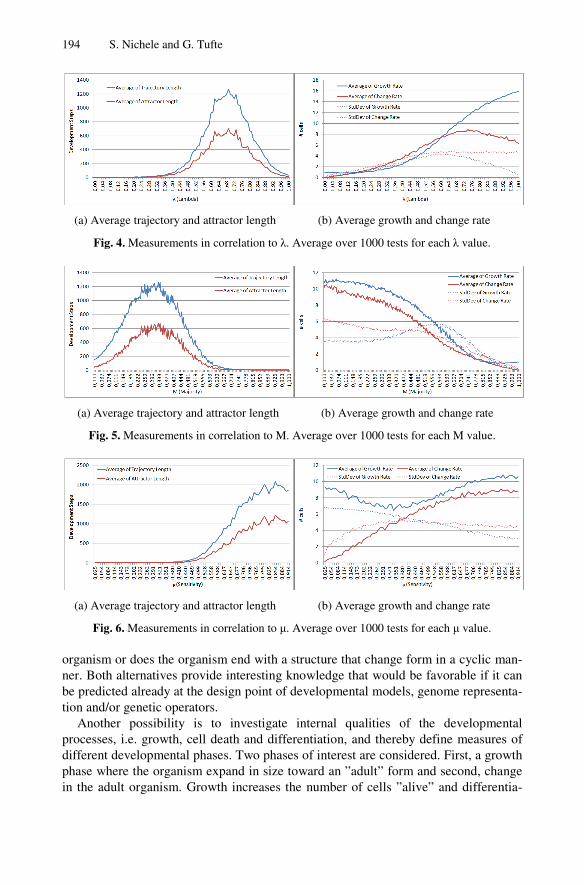
194 S. Nichele and G. Tu
(a) Average trajectory and a
Fig. 4. Measurements in
(a) Average trajectory and a
Fig. 5. Measurements in
(a) Average trajectory and a
Fig. 6. Measurements in
organism or does the organner. Both alternatives provibe predicted already at the dtion and/or genetic operator
Another possibility is processes, i.e. growth, cell different developmental phaphase where the organism ein the adult organism. Gro
ufte
attractor length (b) Average growth and change rate
n correlation to λ. Average over 1000 tests for each λ value.
attractor length (b) Average growth and change rate
correlation to M. Average over 1000 tests for each M value.
attractor length (b) Average growth and change rate
n correlation to μ. Average over 1000 tests for each μ value.
nism end with a structure that change form in a cyclic mide interesting knowledge that would be favorable if it design point of developmental models, genome represenrs. to investigate internal qualities of the developmendeath and differentiation, and thereby define measures
ases. Two phases of interest are considered. First, a growexpand in size toward an ”adult” form and second, chawth increases the number of cells ”alive” and differen
man-can nta-
ntal s of wth
ange ntia-
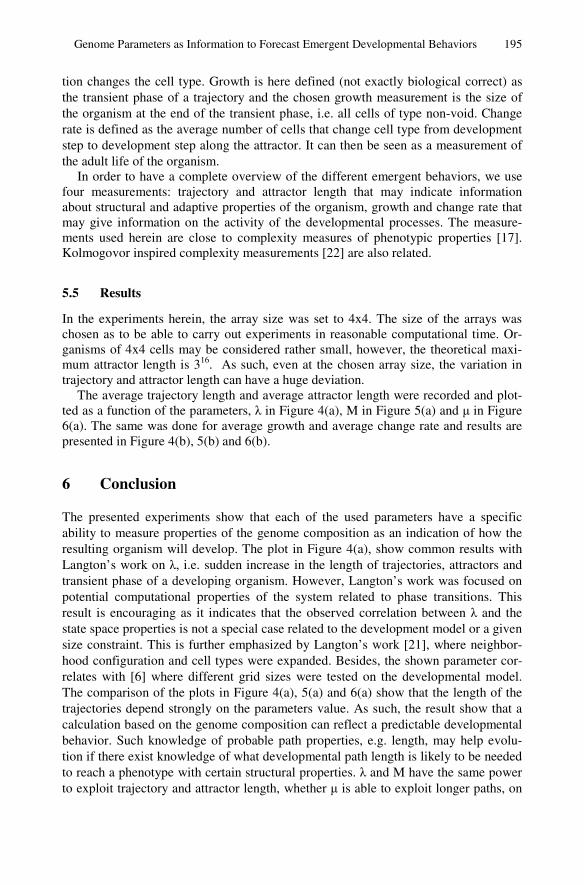
Genome Parameters as Information to Forecast Emergent Developmental Behaviors 195
tion changes the cell type. Growth is here defined (not exactly biological correct) as the transient phase of a trajectory and the chosen growth measurement is the size of the organism at the end of the transient phase, i.e. all cells of type non-void. Change rate is defined as the average number of cells that change cell type from development step to development step along the attractor. It can then be seen as a measurement of the adult life of the organism.
In order to have a complete overview of the different emergent behaviors, we use four measurements: trajectory and attractor length that may indicate information about structural and adaptive properties of the organism, growth and change rate that may give information on the activity of the developmental processes. The measure-ments used herein are close to complexity measures of phenotypic properties [17]. Kolmogovor inspired complexity measurements [22] are also related.
5.5 Results
In the experiments herein, the array size was set to 4x4. The size of the arrays was chosen as to be able to carry out experiments in reasonable computational time. Or-ganisms of 4x4 cells may be considered rather small, however, the theoretical maxi-mum attractor length is 316. As such, even at the chosen array size, the variation in trajectory and attractor length can have a huge deviation.
The average trajectory length and average attractor length were recorded and plot-ted as a function of the parameters, λ in Figure 4(a), M in Figure 5(a) and μ in Figure 6(a). The same was done for average growth and average change rate and results are presented in Figure 4(b), 5(b) and 6(b).
6 Conclusion
The presented experiments show that each of the used parameters have a specific ability to measure properties of the genome composition as an indication of how the resulting organism will develop. The plot in Figure 4(a), show common results with Langton’s work on λ, i.e. sudden increase in the length of trajectories, attractors and transient phase of a developing organism. However, Langton’s work was focused on potential computational properties of the system related to phase transitions. This result is encouraging as it indicates that the observed correlation between λ and the state space properties is not a special case related to the development model or a given size constraint. This is further emphasized by Langton’s work [21], where neighbor-hood configuration and cell types were expanded. Besides, the shown parameter cor-relates with [6] where different grid sizes were tested on the developmental model. The comparison of the plots in Figure 4(a), 5(a) and 6(a) show that the length of the trajectories depend strongly on the parameters value. As such, the result show that a calculation based on the genome composition can reflect a predictable developmental behavior. Such knowledge of probable path properties, e.g. length, may help evolu-tion if there exist knowledge of what developmental path length is likely to be needed to reach a phenotype with certain structural properties. λ and M have the same power to exploit trajectory and attractor length, whether μ is able to exploit longer paths, on
196 S. Nichele and G. Tufte
average. An interpretation of such result is that μ can be used to guide towards part of the search space where genomes with long attractors are more likely to be found.
The results in Figure 4(b), 5(b) and 6(b), further emphases a relation between the measurements of genomic composition and developmental behavior. In Figure 4(b) the growth rate shows that for low values of λ the transient phase of the developmen-tal path is rather short. Genomes with this property have a rather high probability of short developmental time with a point or short attractor. This knowledge is useful if a requirement is to develop stable organisms. Figure 5(b) shows that parameter M has the same ability as λ to represent growth rate of developing organisms but could be better suited to discover organism with higher number of structure and shape changes, especially for low M values. Figure 6(b) show that the usage of μ as measurement of genomic composition could accentuate the possibility to find organisms that develop at a higher rate with low changes in their attractor, thus being quite stable with few changes in form. Again, such knowledge could be helpful at the system design stage if information on the desired target phenotype is known.
Comparing the results in Figure 4, 5 and 6, it is possible to observe that if two or more parameters would be used together, it could be possible to compose develop-mental behaviors that are not achievable with a single parameter, e.g. low λ value to achieve short attractor lengths and low μ value to obtain higher growth rate. In terms of evolvability, it could be possible to add several parameters in the fitness function. However, evolving behaviors instead of looking at the effect would require a different experimental approach than the one used herein.
Moreover, when it comes to adaptivity and evolution, the results herein show that genomes with a given parameter value will most likely mutate to genomes with simi-lar developmental behavior as long as the mutation result in an offspring with similar parameter value. Parameters could then be used to guide evolution towards favorable areas of the solution space and then remain in that area without jumping in a complete different region of the hyperspace where desired developmental behaviors are less likely to be found.
References
1. Binder, P. M.: A Phase Diagram for Elementary Cellular Automata. Complex Systems, 7, 241-247 (1993)
2. Binder, P.M.: Parametric Ordering of Complex Systems. Physical Review E, vol. 49 n. 3, pp. 2023-2025 (1994)
3. De Oliveira, G., De Oliveira, P., Omar, N.: Guidelines for Dynamics-based Parametriza-tion of One-Dimensional Cellular Automata Rule Space. John Wiley & Sons, Inc. Vol. 6, No. 2 Complexity (2001)
4. De Oliveira, G., De Oliveira, P., Omar, N.: Definition and Application of a Five-Parameter Characterization of One-Dimensional Cellular Automata Rule Space. MIT, Artificial Life7: pp. 277-301 (2001)
5. Li, W.: Phenomenology of Nonlocal Cellular Automata. Santa Fe Institute. Journal of Sta-tistical Physics, 68(5-6): 829-882 (1992)
6. Tufte, G., Nichele, S.: On the correlations between developmental diversity and genomic composition. GECCO 2011, ACM, pp. 1507-1514 (2011)
Genome Parameters as Information to Forecast Emergent Developmental Behaviors 197
7. Nichele, S., Tufte, G.: Trajectories and Attractors as Specification for the Evolution of Be-havior in Cellular Automata. IEEE CEC 2010 pp. 4441-4448 (2010)
8. Beer, R.D.: A dynamical systems perspective on agent-environment interaction. Artificial Intelligence, 1–2(72):173–215 (1995)
9. Bentley, P.J., Kumar, S.: Three ways to grow designs: A comparison of embryogenies for an evolutionary design problem. GECCO 1999, pages 35–43 (1999)
10. Cussat-Blanc, S., Luga, H., Duthen, Y.: From single cell to simple creature morphology and metabolism. In S. Bullock, J. Noble, R.Watson, and M. A. Bedau, editors, Artificial Life XI, pages 134–141. MIT Press, Cambridge, MA (2008)
11. Eggenberger, P.: Evolving morphologies of simulated 3d organisms based on differential gene expression. In 4th Artificial Life conference, pages 205–213. MIT press (1997)
12. Fleischer, K., Barr, A.H.: A simulation testbed for the study of multicellular development: The multiple mechanisms of morphogenesis. In 3rd Artificial Life conference, pages 389–416. Addison-Wesley (1993)
13. Forrest, S.: Emergent Computation. MIT Press (1991) 14. Gordon, T.G.W.: Exploring models of development for evolutionary circuit design. IEEE
CEC 2003, pages 2050–2057. IEEE (2003) 15. Hall, B.K., Pearson, R.D., M¨uller, G.B.: Environment, development, and Evolution To-
ward a Synthesis. The Vienna Series in Theoretical Biology. MIT-Press (2004) 16. Kitano, H.: Building complex systems using development process: An engineering ap-
proach. In Evolvable Systems: from Biology to Hardware, ICES, LNCS, pages 218–229. Springer (1998)
17. Kowaliw, T.: Measures of complexity for artificial embryogeny. GECCO 2008. ACM (2008)
18. Kowaliw, T., Grogono, P., Kharma, N.: Environment as a spatial constraint on the growth of structural form. GECCO 2007, pages 1037–1044, New York, NY, USA (2007).
19. Kumar, S., Bentley, P.J.: Biologically inspired evolutionary development. In 5th Interna-tional Conference on Evolvable Systems (ICES03), Lecture Notes in Computer Science, pages 57–68. Springer (2003)
20. Langton, C.G.: Self-reproduction in cellular automata. Physica D, 10:135–144 (1984) 21. Langton, C.G.: Computation at the edge of chaos: phase transitions and emergent compu-
tation. In S. Forrest, editor, Emergent Computation, pages 12–37. MIT Press (1991) 22. Lehre, P.K., Haddow, P.C.: Developmental mappings and phenotypic complexity. In Con-
gress on Evolutionary Computation (CEC2003), pages 62–68. IEEE (2003) 23. Miller, J.F.: Evolving a self-repairing, self-regulating, french flag organism. GECCO 2004,
Lecture Notes in Computer Science, pages 129–139. Springer (2004) 24. Miller, J.F., Banzhaf, W.: Evolving the program for a cell: from french flag to boolean cir-
cuits. In S. Kumar and P. J. Bentley, editors, On Growth, Form and Computers, pages 278–301. Elsevier Limited Oxford UK (2003)
25. Mitchell, M. Hraber, P.T., Crutchfield, J.P.: revisiting the egde of chaos: Evolving cellular automata to perform computations. Complex Systems, 7:89–130. Santa Fe Institute Work-ing Paper 93-03-014 (1993)
26. Packard, N.H.: Dynamic Patterns in Complex Systems, chapter Adaptation Toward the Edge of Chaos, pages 293–301. World Scientific (1988)
27. Tufte, G.: Evolution, development and environment toward adaptation through phenotypic plasticity and exploitation of external information. S. Bullock, J. Noble, R. Watson, and M. A. Bedau, editors, Artificial Life XI, pages 624–631. MIT Press, Cambridge, MA (2008)
28. West-Eberhard, M.J.: Developmental Plasticity and Evolution. Oxford Univ. Press (2003) 29. Wolfram, S: Universality and complexity in CA. Physica D, 10(1-2):1–35 (1984)
Paper B.1
Measuring Phenotypic Structural Complexity
of Artificial Cellular Organisms Approximation of Kolmogorov Complexity with Lempel-Ziv Compression
S. Nichele and G. Tufte
4th
International Conference on Innovations in Bio-Inspired Computing and
Applications, IBICA 2013
August 22 - 24, 2013
Ostrava, Czech Republic

74
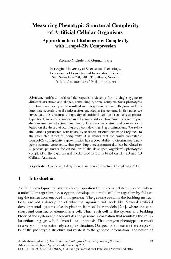
A. Abraham et al. (eds.), Innovations in Bio-inspired Computing and Applications, Advances in Intelligent Systems and Computing 237,
23
DOI: 10.1007/978-3-319-01781-5_3, © Springer International Publishing Switzerland 2014
Measuring Phenotypic Structural Complexity of Artificial Cellular Organisms
Approximation of Kolmogorov Complexity with Lempel-Ziv Compression
Stefano Nichele and Gunnar Tufte
Norwegian University of Science and Technology, Department of Computer and Information Science,
Sem Selandsvei 7-9, 7491, Trondheim, Norway {nichele,gunnart}@idi.ntnu.no
Abstract. Artificial multi-cellular organisms develop from a single zygote to different structures and shapes, some simple, some complex. Such phenotypic structural complexity is the result of morphogenesis, where cells grow and dif-ferentiate according to the information encoded in the genome. In this paper we investigate the structural complexity of artificial cellular organisms at pheno-typic level, in order to understand if genome information could be used to pre-dict the emergent structural complexity. Our measure of structural complexity is based on the theory of Kolmogorov complexity and approximations. We relate the Lambda parameter, with its ability to detect different behavioral regimes, to the calculated structural complexity. It is shown that the easily computable Lempel-Ziv complexity approximation has a good ability to discriminate emer-gent structural complexity, thus providing a measurement that can be related to a genome parameter for estimation of the developed organism’s phenotypic complexity. The experimental model used herein is based on 1D, 2D and 3D Cellular Automata.
Keywords: Developmental Systems, Emergence, Structural Complexity, CAs.
1 Introduction
Artificial developmental systems take inspiration from biological development, where a unicellular organism, i.e. a zygote, develops to a multi-cellular organism by follow-ing the instructions encoded in its genome. The genome contains the building instruc-tions and not a description of what the organism will look like. Several artificial developmental systems take inspiration from cellular models [2-4], where the con-struct and constructor element is a cell. Thus, each cell in the system is a building block of the system and encapsulates the genome information that regulates the cellu-lar actions, e.g. growth, differentiation, apoptosis. The emergent phenotype can result in a very simple or extremely complex structure. Our goal is to measure the complexi-ty of the phenotypic structure and relate it to the genome information. The notion of
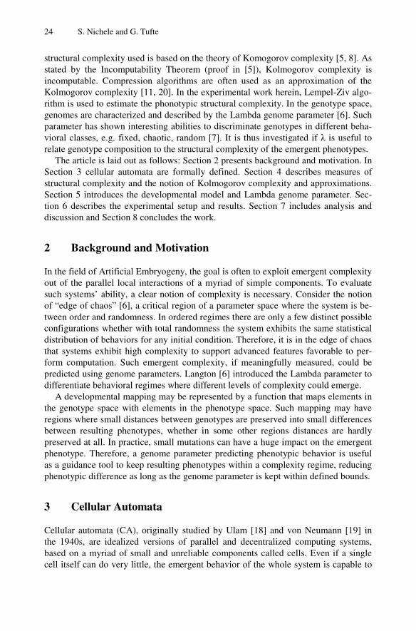
24 S. Nichele and G. Tufte
structural complexity used is based on the theory of Komogorov complexity [5, 8]. As stated by the Incomputability Theorem (proof in [5]), Kolmogorov complexity is incomputable. Compression algorithms are often used as an approximation of the Kolmogorov complexity [11, 20]. In the experimental work herein, Lempel-Ziv algo-rithm is used to estimate the phonotypic structural complexity. In the genotype space, genomes are characterized and described by the Lambda genome parameter [6]. Such parameter has shown interesting abilities to discriminate genotypes in different beha-vioral classes, e.g. fixed, chaotic, random [7]. It is thus investigated if λ is useful to relate genotype composition to the structural complexity of the emergent phenotypes.
The article is laid out as follows: Section 2 presents background and motivation. In Section 3 cellular automata are formally defined. Section 4 describes measures of structural complexity and the notion of Kolmogorov complexity and approximations. Section 5 introduces the developmental model and Lambda genome parameter. Sec-tion 6 describes the experimental setup and results. Section 7 includes analysis and discussion and Section 8 concludes the work.
2 Background and Motivation
In the field of Artificial Embryogeny, the goal is often to exploit emergent complexity out of the parallel local interactions of a myriad of simple components. To evaluate such systems’ ability, a clear notion of complexity is necessary. Consider the notion of “edge of chaos” [6], a critical region of a parameter space where the system is be-tween order and randomness. In ordered regimes there are only a few distinct possible configurations whether with total randomness the system exhibits the same statistical distribution of behaviors for any initial condition. Therefore, it is in the edge of chaos that systems exhibit high complexity to support advanced features favorable to per-form computation. Such emergent complexity, if meaningfully measured, could be predicted using genome parameters. Langton [6] introduced the Lambda parameter to differentiate behavioral regimes where different levels of complexity could emerge.
A developmental mapping may be represented by a function that maps elements in the genotype space with elements in the phenotype space. Such mapping may have regions where small distances between genotypes are preserved into small differences between resulting phenotypes, whether in some other regions distances are hardly preserved at all. In practice, small mutations can have a huge impact on the emergent phenotype. Therefore, a genome parameter predicting phenotypic behavior is useful as a guidance tool to keep resulting phenotypes within a complexity regime, reducing phenotypic difference as long as the genome parameter is kept within defined bounds.
3 Cellular Automata
Cellular automata (CA), originally studied by Ulam [18] and von Neumann [19] in the 1940s, are idealized versions of parallel and decentralized computing systems, based on a myriad of small and unreliable components called cells. Even if a single cell itself can do very little, the emergent behavior of the whole system is capable to
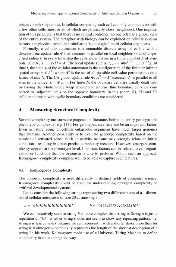
Measuring Phenotypic Structural Complexity of Artificial Cellular Organisms 25
obtain complex dynamics. In cellular computing each cell can only communicate with a few other cells, most or all of which are physically close (neighbors). One implica-tion of this principle is that there is no central controller; no one cell has a global view of the entire system. The metaphor with biology can be exploited on cellular systems because the physical structure is similar to the biological multi-cellular organisms.
Formally, a cellular automaton is a countable discrete array of cells i with a discrete-time update rule Φ that executes in parallel on local neighborhoods of a spe-cified radius r. In every time step the cells allow values in a finite alphabet A of sym-bols: σi
t ∈ {0, 1, ..., k-1} ≡ A. The local update rule is σit + 1 = Φ(σi - r
t , …, σi + rt). At
time t, the state st of the cellular automaton is the configuration of the finite or infinite spatial array: st ∈ AN, where AN is the set of all possible cell value permutations on a lattice of size N. The CA global update rule Φ: AN → AN executes Φ in parallel to all sites in the lattice: st = Φ st - 1. For finite N, the boundary cells are usually dealt with by having the whole lattice wrap around into a torus, thus boundary cells are con-nected to “adjacent" cells on the opposite boundary. In this paper, 1D, 2D and 3D cellular automata with cyclic boundary conditions are considered.
4 Measuring Structural Complexity
Several complexity measures are proposed in literature, both to quantify genotype and phenotype complexity, e.g. [17]. For genotypes, size may not be an important factor. Even in nature, some unicellular eukaryotic organisms have much larger genomes than humans. Another possibility is to evaluate genotype complexity based on the number of activated genes. Such an activity measure may strongly relate on initial conditions, resulting in a non-precise complexity measure. However, emergent com-plexity appears at the phenotype level. Important factors can be related to cell organi-zation or functions that the organism is able to perform. Within such an approach Kolmogorov complexity complies well to be able to capture such features.
4.1 Kolmogorov Complexity
The notion of complexity is used differently in distinct fields of computer science. Kolmogorov complexity could be used for understanding emergent complexity in artificial developmental systems.
Let us consider the following strings representing two different states of a 1 dimen-sional cellular automaton of size 20 at time step t:
a = “01010101010101010101” b = “01234567894978253167”
We can intuitively see that string b is more complex than string a. String a is just a repetition of “01” whether string b does not seem to show any repeating pattern, i.e. string a is less complex because we can represent it with a shorter description than for string b. Kolmogorov complexity represents the length of the shortest description of a string. In his work, Kolmogorov made use of a Universal Turing Machine to define complexity in an unambiguous way.
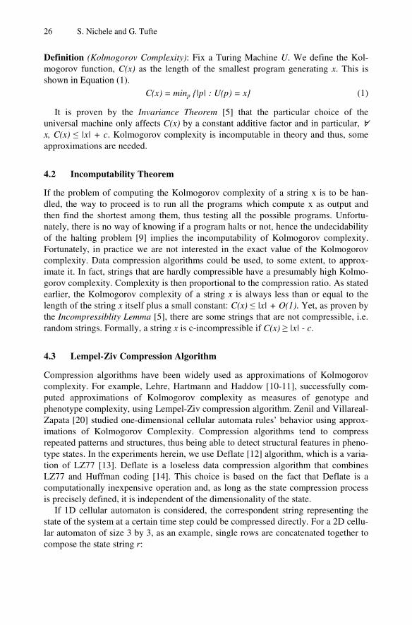
26 S. Nichele and G. Tufte
Definition (Kolmogorov Complexity): Fix a Turing Machine U. We define the Kol-mogorov function, C(x) as the length of the smallest program generating x. This is shown in Equation (1).
C(x) = minp {|p| : U(p) = x} (1)
It is proven by the Invariance Theorem [5] that the particular choice of the universal machine only affects C(x) by a constant additive factor and in particular, ∀ x, C(x) ≤ |x| + c. Kolmogorov complexity is incomputable in theory and thus, some approximations are needed.
4.2 Incomputability Theorem
If the problem of computing the Kolmogorov complexity of a string x is to be han-dled, the way to proceed is to run all the programs which compute x as output and then find the shortest among them, thus testing all the possible programs. Unfortu-nately, there is no way of knowing if a program halts or not, hence the undecidability of the halting problem [9] implies the incomputability of Kolmogorov complexity. Fortunately, in practice we are not interested in the exact value of the Kolmogorov complexity. Data compression algorithms could be used, to some extent, to approx-imate it. In fact, strings that are hardly compressible have a presumably high Kolmo-gorov complexity. Complexity is then proportional to the compression ratio. As stated earlier, the Kolmogorov complexity of a string x is always less than or equal to the length of the string x itself plus a small constant: C(x) ≤ |x| + O(1). Yet, as proven by the Incompressiblity Lemma [5], there are some strings that are not compressible, i.e. random strings. Formally, a string x is c-incompressible if C(x) ≥ |x| - c.
4.3 Lempel-Ziv Compression Algorithm
Compression algorithms have been widely used as approximations of Kolmogorov complexity. For example, Lehre, Hartmann and Haddow [10-11], successfully com-puted approximations of Kolmogorov complexity as measures of genotype and phenotype complexity, using Lempel-Ziv compression algorithm. Zenil and Villareal-Zapata [20] studied one-dimensional cellular automata rules’ behavior using approx-imations of Kolmogorov Complexity. Compression algorithms tend to compress repeated patterns and structures, thus being able to detect structural features in pheno-type states. In the experiments herein, we use Deflate [12] algorithm, which is a varia-tion of LZ77 [13]. Deflate is a loseless data compression algorithm that combines LZ77 and Huffman coding [14]. This choice is based on the fact that Deflate is a computationally inexpensive operation and, as long as the state compression process is precisely defined, it is independent of the dimensionality of the state.
If 1D cellular automaton is considered, the correspondent string representing the state of the system at a certain time step could be compressed directly. For a 2D cellu-lar automaton of size 3 by 3, as an example, single rows are concatenated together to compose the state string r:
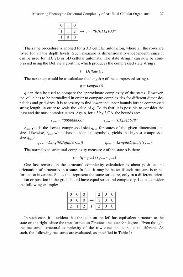
Measuring Phenotypic Structural Complexity of Artificial Cellular Organisms 27
0 1 0
1 1 2 → r = “010112100”
1 0 0
The same procedure is applied for a 3D cellular automaton, where all the rows are
listed for all the depth levels. Such measure is dimensionality-independent, since it can be used for 1D, 2D or 3D cellular automata. The state string r can now be com-pressed using the Deflate algorithm, which produces the compressed state string t.
t = Deflate (r)
The next step would be to calculate the length q of the compressed string t.
q = Length (t)
q can then be used to compare the approximate complexity of the states. However, the value has to be normalized in order to compare complexities for different dimensio-nalities and grid sizes. It is necessary to find lower and upper bounds for the compressed string length, in order to scale the value of q. To do that, it is possible to consider the least and the most complex states. Again, for a 3 by 3 CA, the bounds are:
rmin = ”000000000” rmax = ”012345678”
rmin yields the lowest compressed size qmin for states of the given dimension and size. Likewise, rmax which has no identical symbols, yields the highest compressed size qmax:
qmin = Length(Deflate(rmin)) qmax = Length(Deflate(rmax))
The normalized structural complexity measure c of the state s is then:
c = (q - qmin) / (qmax - qmin)
One last remark on the structural complexity calculation is about position and orientation of structures in a state. In fact, it may be better if such measure is trans-formation invariant. States that represent the same structure, only in a different orien-tation or position in the grid, should have equal structural complexity. Let us consider the following example:
0 0 0 2 0 0
0 0 0 → 1 0 0
2 1 2 T 2 0 0
In such case, it is evident that the state on the left has equivalent structure to the
state on the right, since the transformation T rotates the state 90 degrees. Even though, the measured structural complexity of the row-concatenated-state is different. As such, the following measures are evaluated, as specified in Table 1:
28 S. Nichele and G. Tufte
Table 1. Complexity measures
1 Simple Deflate compression
The CA state is represented as a concatenated string and directly compressed.
2 Average of all
rotations The CA state is rotated in all the possible orientations and the correspondent state strings are compressed. The average is computed.
3 Average of all
translations The CA state is shifted in all the possible positions and the correspondent state strings are compressed. The average is computed.
4 Rotations + translations
Both point 2 and 3. The CA state is rotated in all the possible orientations. Each of them is shifted in all the possible positions and the correspondent state strings are compressed. The overall average is computed.
5 Cellular Developmental Model
The developmental model used in this work is an embryomorphic system [1] based on cellular automata, where the goal is the self-assembly of cells from a single zygote which holds the complete genotype information. A CA can be considered as a devel-oping organism, where the genome specification and the gene regulation information control the cells’ growth, differentiation and apoptosis. The global emergent behavior of the system is then represented by the emerging phenotype, which is subject to size, shape and structure modifications along the developmental process.
The experimental work is conducted on cellular automata with different dimensio-nalities, 1 – 3, and neighborhood configurations, 3 – 7.
All CAs have cyclic boundary conditions. Each cell has 3 possible states (cell type 0: empty/dead cell, cell type 1 and cell type 2). The grid is initialized with a cell of type 1 (zygote) in the middle of the grid and develops according to a genotype based on a cellular developmental table that fully specifies all the possible regulatory input combinations, i.e. all 3n neighborhood configurations are explicitly represented (n represents the neighborhood size). To ensure that cells will not materialize where there are no other cells around, a restriction has been set in the developmental table: if all the neighbors of an empty cell are empty, the cell will be empty also in the follow-ing development step. A more detailed description of the developmental model is given in [15-16].
During the development process, a unicellular organism grows to a multi-cellular organism. Two different life phases are identified: the transient phase and the attrac-tor. The transient phase begins with the initial state of the CA (zygote) and ends when the organism reaches its adult form and an attractor begins. Note that this definition is not biologically correct. The attractor represents the time lapse between two repeti-tions of the same state, i.e. the same state is encountered twice. A complete trajectory is then defined as the sum of transient phase and attractor.
The Lambda Genome Parameter obtained from the genome information can be used to estimate the dynamic behavior of the system and thus can be related to the emergent complexity of the phenotype. Langton [6] studied the parameter λ as a
Measuring Phenotypic Structural Complexity of Artificial Cellular Organisms 29
measure of the activity level of the system. λ has shown to be particularly well suited to discriminate genotypes that will develop phenotypes in different behavioral classes, e.g. fixed, chaotic, random [7]. Lambda is calculated out of the regulative outcome of the developmental table, i.e. the output at time t+1 based on a specific neighborhood configuration at time t. According to Langton’s definition, a quiescent state must be chosen. We choose the empty cell (type 0) as the quiescent state. λ is then calculated according to Equation 2, where n represents the number of transitions to the quiescent state, K is the number of cell types (three in our case) and N is the neighborhood size, as defined in Table 2. λ (2)
Langton observed that the basic functions required for computation (transmission, storage and modification of information) are more likely to be achieved in the vicinity of phase transitions between ordered and disordered dynamics (edge of chaos). He hypothesized that it is easier to find genotypes capable of complex computation in a region where the value of λ is critical.
In the experiments herein, genomes are generated in the whole Lambda spectrum, from 0 to 1, using a similar method to Langton’s random table method [6], i.e. for every entry in the developmental table, with probability (1-λ) the cell type at the next developmental step is quiescent (type 0); with probability (λ), the cell type at the next developmental step is generated by a uniform random distribution among the other cell types (type 1 or 2).
Previous work [16] has shown that Lambda is able to discriminate genotypes that will end up with very long or extremely short trajectories and attractors. In this paper we investigate relationship between λ, as a genotype measurement, and emergent structural complexity of the corresponding phenotypes.
6 Experimental Setup
Two different sets of experiments are conducted. First, the four different complexity measures in Table 1 are tested. 100 developmental tables are generated for each λ value with granularity 0.01. The correspondent genotypes are developed starting from a single cell on different cellular architectures (1, 2 or 3D with 3, 5 or 7 neighbors), as specified in Table 2, experiment 1. The structural complexity is then measured for the whole trajectory and for the attractor.
Plots from Figure 1.1 to 1.7 show the results for each configuration in Table 2 – experiment 1, where the four lines represent the complexity measures in Table 1. The x-axes plots the whole Lambda spectrum whether the y-axes is the measured structur-al complexity.
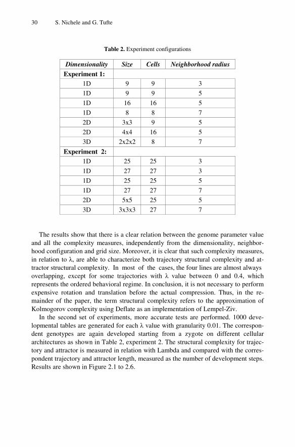
30 S. Nichele and G. Tufte
Table 2. Experiment configurations
Dimensionality Size Cells Neighborhood radius
Experiment 1: 1D 9 9 3
1D 9 9 5
1D 16 16 5
1D 8 8 7
2D 3x3 9 5
2D 4x4 16 5
3D 2x2x2 8 7
Experiment 2: 1D 25 25 3
1D 27 27 3
1D 25 25 5
1D 27 27 7
2D 5x5 25 5
3D 3x3x3 27 7
The results show that there is a clear relation between the genome parameter value
and all the complexity measures, independently from the dimensionality, neighbor-hood configuration and grid size. Moreover, it is clear that such complexity measures, in relation to λ, are able to characterize both trajectory structural complexity and at-tractor structural complexity. In most of the cases, the four lines are almost always overlapping, except for some trajectories with λ value between 0 and 0.4, which represents the ordered behavioral regime. In conclusion, it is not necessary to perform expensive rotation and translation before the actual compression. Thus, in the re-mainder of the paper, the term structural complexity refers to the approximation of Kolmogorov complexity using Deflate as an implementation of Lempel-Ziv.
In the second set of experiments, more accurate tests are performed. 1000 deve-lopmental tables are generated for each λ value with granularity 0.01. The correspon-dent genotypes are again developed starting from a zygote on different cellular architectures as shown in Table 2, experiment 2. The structural complexity for trajec-tory and attractor is measured in relation with Lambda and compared with the corres-pondent trajectory and attractor length, measured as the number of development steps. Results are shown in Figure 2.1 to 2.6.
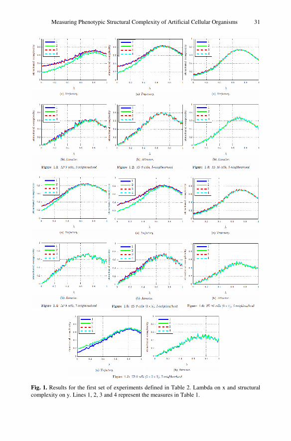
Measuring Phenotypic Structural Complexity of Artificial Cellular Organisms 31
Fig. 1. Results for the first set of experiments defined in Table 2. Lambda on x and structural complexity on y. Lines 1, 2, 3 and 4 represent the measures in Table 1.
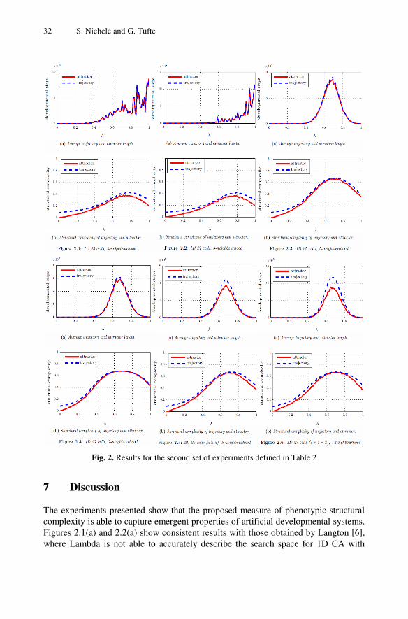
32 S. Nichele and G. Tufte
Fig. 2. Results for the second set of experiments defined in Table 2
7 Discussion
The experiments presented show that the proposed measure of phenotypic structural complexity is able to capture emergent properties of artificial developmental systems. Figures 2.1(a) and 2.2(a) show consistent results with those obtained by Langton [6], where Lambda is not able to accurately describe the search space for 1D CA with
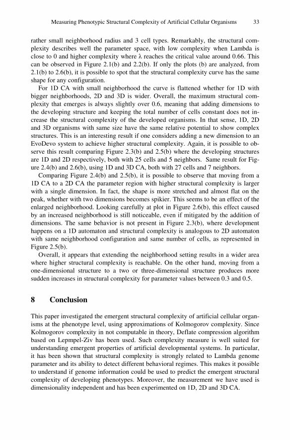
Measuring Phenotypic Structural Complexity of Artificial Cellular Organisms 33
rather small neighborhood radius and 3 cell types. Remarkably, the structural com-plexity describes well the parameter space, with low complexity when Lambda is close to 0 and higher complexity where λ reaches the critical value around 0.66. This can be observed in Figure 2.1(b) and 2.2(b). If only the plots (b) are analyzed, from 2.1(b) to 2.6(b), it is possible to spot that the structural complexity curve has the same shape for any configuration.
For 1D CA with small neighborhood the curve is flattened whether for 1D with bigger neighborhoods, 2D and 3D is wider. Overall, the maximum structural com-plexity that emerges is always slightly over 0.6, meaning that adding dimensions to the developing structure and keeping the total number of cells constant does not in-crease the structural complexity of the developed organisms. In that sense, 1D, 2D and 3D organisms with same size have the same relative potential to show complex structures. This is an interesting result if one considers adding a new dimension to an EvoDevo system to achieve higher structural complexity. Again, it is possible to ob-serve this result comparing Figure 2.3(b) and 2.5(b) where the developing structures are 1D and 2D respectively, both with 25 cells and 5 neighbors. Same result for Fig-ure 2.4(b) and 2.6(b), using 1D and 3D CA, both with 27 cells and 7 neighbors.
Comparing Figure 2.4(b) and 2.5(b), it is possible to observe that moving from a 1D CA to a 2D CA the parameter region with higher structural complexity is larger with a single dimension. In fact, the shape is more stretched and almost flat on the peak, whether with two dimensions becomes spikier. This seems to be an effect of the enlarged neighborhood. Looking carefully at plot in Figure 2.6(b), this effect caused by an increased neighborhood is still noticeable, even if mitigated by the addition of dimensions. The same behavior is not present in Figure 2.3(b), where development happens on a 1D automaton and structural complexity is analogous to 2D automaton with same neighborhood configuration and same number of cells, as represented in Figure 2.5(b).
Overall, it appears that extending the neighborhood setting results in a wider area where higher structural complexity is reachable. On the other hand, moving from a one-dimensional structure to a two or three-dimensional structure produces more sudden increases in structural complexity for parameter values between 0.3 and 0.5.
8 Conclusion
This paper investigated the emergent structural complexity of artificial cellular organ-isms at the phenotype level, using approximations of Kolmogorov complexity. Since Kolmogorov complexity in not computable in theory, Deflate compression algorithm based on Lepmpel-Ziv has been used. Such complexity measure is well suited for understanding emergent properties of artificial developmental systems. In particular, it has been shown that structural complexity is strongly related to Lambda genome parameter and its ability to detect different behavioral regimes. This makes it possible to understand if genome information could be used to predict the emergent structural complexity of developing phenotypes. Moreover, the measurement we have used is dimensionality independent and has been experimented on 1D, 2D and 3D CA.
34 S. Nichele and G. Tufte
Another observed result is that structural complexity has shown to be powerful enough to characterize the parameter space even when the dimensionality, number of states per cell and neighborhood size are rather small. In such cases, it would not be possible to obtain predictions about trajectory and attractor length at the genotype stage, thus being uncertain about the emergent behavioral regime of the system. As a future work, it may be possible to exploit the potential of Lambda genome parameter to guide evolution towards desirable levels of phenotypic structural complexity.
Acknowledgment. Thanks to John Anthony for carrying out part of the experimental work during his master thesis project.
References
1. Doursat, R., Sánchez, C., Dordea, R., Fourquet, D., Kowaliw, T.: Embryomorphic engi-neering: emergent innovation through evolutionary development. In: Doursat, R., Sayama, H., Michel, O. (eds.) Morphogenetic Engineering. UCS Series, pp. 275–311. Springer (2012)
2. Kumar, S., Bentley, P.J.: Biologically inspired evolutionary development. In: Tyrrell, A.M., Haddow, P.C., Torresen, J. (eds.) ICES 2003. LNCS, vol. 2606, pp. 57–68. Springer, Heidelberg (2003)
3. Miller, J.F., Banzhaf, W.: Evolving the program for a cell: from French flag to boolean circuits. In: Kumar, S., Bentley, P.J. (eds.) On Growth, Form and Computers, pp. 278–301. Elsevier Limited, Oxford (2003)
4. Tufte, G.: Evolution, development and environment toward adaptation through phenotypic plasticity and exploitation of external information. In: Bullock, S., Noble, J., Watson, R., Bedau, M.A. (eds.) Artificial Life XI, pp. 624–631. MIT Press, Cambridge (2008)
5. Li, M., Vitanyi, P.M.B.: An introduction to Kolmogorov complexity and its applications, 2nd edn. Springer, New York (1997)
6. Langton, C.G.: Computation at the edge of chaos: phase transitions and emergent compu-tation. In: Forrest, S. (ed.) Emergent Computation, pp. 12–37. MIT Press (1991)
7. Wolfram, S.: Universality and complexity in CA. Physica D 10(1-2), 1–35 (1984) 8. Kolmogorov, A.N.: Three approaches to the quantitative definition of information. Prob-
lems Inform. Transmission 1(1), 1–7 (1965) 9. Turing, A.: On computable numbers, with an application to the Entscheidungsproblem.
Proceedings of the London Mathematical Society, Series 2 42, 230–265 (1936) 10. Hartmann, M., Lehre, P.K., Haddow, P.C.: Evolved digital circuits and genome complexi-
ty. In: NASA/DoD Conference on Evolvable Hardware 2005, pp. 79–86. IEEE Press (2005)
11. Lehre, P.K., Haddow, P.C.: Developmental mappings and phenotypic complexity. In: Pro-ceedings of 2003 IEEE CEC, vol. 1, pp. 62–68. IEEE Press (2003)
12. Deutsch, L.P.: DEFLATE Compressed data format specification version 1.3 (1996) 13. Ziv, J., Lempel, A.: A universal algorithm for sequential data compression. IEEE Transac-
tions on Information Theory 23(3), 337–343 (1977) 14. Huffman, D.A.: A method for the construction of minimum-redundancy codes. Proceed-
ings of the I.R.E., 1098–1102 (1952)
Measuring Phenotypic Structural Complexity of Artificial Cellular Organisms 35
15. Tufte, G., Nichele, S.: On the correlations between developmental diversity and genomic composition. In: 13th Annual Genetic and Evolutionary Computation Conference, GECCO 2011, pp. 1507–1514. ACM (2011)
16. Nichele, S., Tufte, G.: Genome parameters as information to forecast emergent develop-mental behaviors. In: Durand-Lose, J., Jonoska, N. (eds.) UCNC 2012. LNCS, vol. 7445, pp. 186–197. Springer, Heidelberg (2012)
17. Kowaliw, T.: Measures of complexity for artificial embryogeny. In: GECCO 2008, pp. 843–850. ACM (2008)
18. Ulam, S.: Los Alamos National Lab 1909-1984, vol. 15(special issue), pp. 1–318. Los Alamos Science, Los Alamos (1987)
19. von Neumann, J.: Theory and organization of complicated automata. In: Burks, A.W. (ed.), pp. 29–87 (2, part one). Based on transcript of lectures delivered at the University of Illinois (December 1949)
20. Zenil, H., Villareal-Zapata, E.: Asymptotic behaviour and ratios of complexity in cellular automata. arXiv/1304.2816 (2013)

88
Paper C.1
Evolution of Incremental Complex Behavior
on Cellular Machines
S. Nichele and G. Tufte
12th European Conference on the Synthesis and Simulation of Living Systems, ECAL
2013
September 2 - 6, 2013
Taormina, Italy

90
Evolution of Incremental Complex Behavior on Cellular Machines
Stefano Nichele1 and Gunnar Tufte1
1 Norwegian University of Science and Technology, Department of Computer and Information Science, Sem Selandsvei 7-9, 7491, Trondheim, Norway
{nichele, gunnart}@idi.ntnu.no
Abstract Complex multi-cellular organisms are the result of evolution over billions of years. Their ability to reproduce and survive through adaptation to selection pressure did not happen suddenly; it required gradual genome evolution that eventually led to an increased emergent complexity. In this paper we investigate the emergence of complexity in cellular machines, using two different evolutionary strategies. The first approach is a conventional genetic algorithm, where the target is the maximum complexity. This is compared to an incremental approach, where complexity is gradually evolved. We show that an incremental methodology could be better suited to help evolution to discover complex emergent behaviors. We also propose the usage of a genome parameter to detect the behavioral regime. The parameter may indicate if the evolving genomes are likely to be able to achieve more complex behaviors, giving information on the evolvability of the system. The experimental model used herein is based on 2-dimensional cellular automata. We show that the incremental approach is promising when evolution targets an increase of complexity.
Introduction Evolved artificial developmental systems’ remarkable range of products, i.e. biological organisms, with variety in form, function and "complexity", all tailored to fill their niche, is an alluring design concept. Such bio-inspired design methodology can be used for any kind of system to create a variety of artifacts that can handle different problems. However, knowledge and methods to be able to exploit similar core processes [14] for the design of artificial organisms are still subjects of exploration and research.
Evolved artificial developmental systems have shown many favorable features that are borrowed from natural biological systems, such as the main subject here, the ability to evolve inherent complexity as a response to evolutionary pressure [27]. Evolvable, or in particular EvoDevo systems are products of bottom-up processes, in contrast to typical top-down engineering design approaches. A system emerging as a product of a bottom-up process can target system properties out-of-bounds for traditional top-down designed artifacts. Self-organization, self-construction, adaptivity, scalability and robustness are all example of such hard to reach properties. In contrast to the open ended evolution in nature, evolution of artificial EvoDevo systems often includes an expressed goal; fitness is a kind of usability [15] measurement. The target functionality is defined and thus placed within some
complexity measure. Such complexity can be defined at sev-eral levels. The complexity of the machine's composition, i.e. the number of components and connections can be quantified. Another complexity measurement may be functionality in terms of information processing. Quantification of complexity in artifacts and biological organism has no common defined unit of measurement or ratio of comparability. However, intuitively there are differences. Such differences can be related to the composition of artifacts/organisms or as a measure of their functionality. If complexity, for an organism, is a measurement of functional properties within its environmental niche, different levels of behavioral complexity can be said to exist. In this context, high complexity is not a goal in itself; it is merely a product of the species adaptation to be able to reproduce. The genetic information included in the genotype and the developmental processes for any particular specie has evolved and diverged through adaptation from the primordial soup. As such, the behavioral complexity of organisms is a product of the evolved interplay between genetic information and developmental processes. As a step toward more knowledge of underlying processes and finding design methodologies for the exploitation of EvoDevo for artificial systems, we investigate how a gradual change in the complexity requirements, in evolutionary time, influence on EvoDevo system's ability to evolve complexity. Further, a variation of Langton's Lambda parameter [16] is used as an indicator of evolutionary genome adaptation to resulting phenotypic complexity. The taken experimental approach uses a kind of incremental complexity evolution to simulate the process of species adaptation to a changing environment requiring growth of complexity. A 2D cellular developmental model based on Cellular Automata (CA) is used in the experiments, so as to be able to visualize artificial organisms’ development in 2 dimensions. In our incremental evolutionary approach, the evolution process tackles the problem of targeting complexity incrementally. Instead of seeking for maximum complexity in the early generations, the problem is divided in sub-problems. Generations are divided in intervals and in every interval the target complexity demand is increased, keeping the target functionality unvaried, i.e. the class of problems is the same. In such way, it may be possible to evolve favorable genes for intermediate complexity levels, which may be beneficial in order to achieve higher complexity in the long term. Since no universally accepted definition of complexity exists, many authors use it implicitly without specifying which
ECAL - General Track
63 ECAL 2013
notion of complexity they are using. Yet, without any common measure of genotype or phenotype complexity, any significant claim is not verifiable. Genome complexity measures may sometimes be unfitting, since the amount of information encoded in the genome is not directly proportional to the complexity of the emergent organisms. Even in nature, some unicellular eukaryotic organisms have much larger genomes than humans. In addition, there are other factors that impact on the organisms’ complexity during their growth, e.g. the environment. One may argue that complexity of an EvoDevo system may be measured in terms of information contained in a genome, by ranking through a Turing machine, by quantifying the capacity for a genome to exploit a provided area of growth, using approximations of Kolmogorov complexity [5, 6, 9]. The used complexity measure is based on compression of CA behavior in terms of trajectory and attractor lengths, a kind of adaptation of principles from Kolmogorov complexity. The article is laid out as follows: background information and motivation on incremental evolution is presented in Section 2. In Section 3 Lambda genome parameter is introduced and in Section 4 the developmental model used in the experiments is described. Section 5 explains the genetic algorithms used herein. The experimental setup is illustrated in Section 6 and in Section 7 the results of the experiments are presented together with a discussion of the ideas and the results. Finally Section 8 concludes the work.
Incremental Evolution A general evolutionary strategy may be too difficult for the evolution system to discover possible solutions directly. Instead, it is possible to learn complex behaviors incrementally, starting from a simple behavior and gradually making the task more challenging [1]. Incremental evolutionary approaches have been used successfully to evolve complex behaviors step by step. Many studies investigated the training of artificial neural networks with Genetic Algorithms (GAs), in order to evolve robots controller able to perform complex action sequences, e.g. complex light switching behavior [2] or robot duels controllers [3]. This approach has shown interesting results, being able to evolve converged populations to the new task. On the other hand, conventional evolutionary methods may have too high selective pressure in the early stages of the evolution, getting the GA blocked in an unfruitful area of the search space. If the population is first evolved to an easier behavior, it may be possible to discover and access a region of the solution space where even more complex behaviors are more likely to be found. As such, the ultimate complex behavior may be reached incrementally by evolving a sequence of intermediate behaviors with growing complexity:
Behavior 1 B 2 …. B n-1 B n
In this way, genotypes are evolved gradually and the search is driven on solutions that are likely to benefit and retain existing capabilities. Conventional evolution tends to fluctuate between idiosyncratic but still not interesting solutions [12]. Incremental evolution may foster continuing innovation by elaborating on available solutions.
Genome Parameter: λ In our cellular developmental model, we are aiming to target complex phenotypic properties. Attractor length, i.e. development reaches a structure or state that is stable by self-regulation (point attractor) or a dynamic phenotypic structure that is self-reorganizing (cyclic attractor), is the chosen metric. The strategy is therefore to evolve intermediate genotypes that develop and express specific attractor lengths. Every fixed number of generations, we increase the sought attractor length value to increment the complexity demand. In terms of evolvability, since we want to investigate if the evolving genotypes are able to evolve and develop more complex phenotypes, we attempt to measure the behavioral regime using a genome parameter. Parameters obtained from the genome information can be used to estimate the dynamic behavior of the system. In this work, the genotypes are represented as a transition rule table, where developmental actions are defined as a function of the neighborhood configuration (see next chapter for details). In this way, it is possible to analyze the different developmental actions and calculate parameters obtained from the genome table. Several genome parameters have been previously proposed in order to measure genotype properties. Langton [16] studied a parameter λ as a measure of the activity level of the system and its disorder. A similar parameter, neighborhood dependent, is Absolute Activity presented by de Oliveira [20]. Li [21] introduced Mean Field Parameters to monitor if the majority of the regulatory actions follow the “mean” configuration. de Oliveira [20] presented a very similar parameter called Neighborhood Dominance. Binder [22, 23] introduced the Sensitivity parameter which measures the number of changes in the output of the transition table based on a change in the neighborhood, one cell at a time, over all the possible neighborhoods of the rule being considered. This has also being studied by de Oliveira [24, 20] as Context Dependence. Different properties of genome parameters have been investigated in details in [11]. In particular, the λ parameter has shown interesting abilities to discriminate genotypes in different behavioral classes, e.g. fixed, chaotic, random [13]. As such, we monitor the λ value along the evolutionary process. λ is calculated according to Equation 1.
N
N
KnK
(1)
n represents the number of transitions to the quiescent state (i.e. inactive or dead state), K is the number of cells types and N is the neighborhood size (see following section for details).
Cellular Developmental Model The developmental model used in this work is a minimalistic cellular developmental model based on cellular automata, similar to cellular models used in [25, 26, 19]. The system herein is close to the field of Morphogenetic Engineering [7], where the goal is “self-architecturing” systems. In embryomorphic systems [8], the approach is based on embryogenesis: the self-assembly of myriads of cells starting from a single zygote which holds the complete genotype information.
ECAL - General Track
ECAL 2013 64
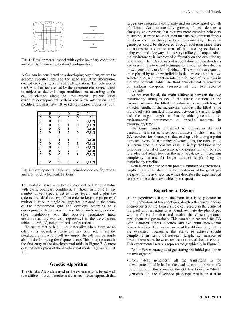
Fig. 1: Developmental model with cyclic boundary conditions and von Neumann neighborhood configuration.
A CA can be considered as a developing organism, where the genome specifications and the gene regulation information control the cells’ growth and differentiation. The behavior of the CA is then represented by the emerging phenotype, which is subject to size and shape modifications, according to the cellular changes along the developmental process. Such dynamic developmental system can show adaptation, self-modification, plasticity [18] or self-replication properties [17].
Fig. 2: Developmental table with neighborhood configurations and relative developmental actions.
The model is based on a two-dimensional cellular automaton with cyclic boundary conditions, as shown in Figure 1. The number of cell types is set to three (type 1 and 2 plus the quiescent or dead cell type 0) in order to keep the property of multicellularity. A single cell (zygote) is placed in the centre of the development grid and develops according to a developmental table based on von Neumann’s neighborhood (five neighbors). All the possible regulatory input combinations are explicitly represented in the development table, i.e. 243 (35) neighborhood configurations. To ensure that cells will not materialize where there are no other cells around, a restriction has been set: if all the neighbors of an empty cell are empty, the cell will be empty also in the following development step. This is represented in the first entry of the developmental table in Figure 2. A more detailed description of the development model is given in [10, 11].
Genetic Algorithm The Genetic Algorithm used in the experiments is tested with two different fitness functions: a classical fitness approach that
targets the maximum complexity and an incremental growth of fitness. An incrementally growing fitness denotes a changing environment that requires more complex behaviors to survive. It must be underlined that the two different fitness functions could in theory perform the same way. The same genotypes could be discovered through evolution since there are no restrictions in the areas of the search space that are being explored. Anyway, this is very unlikely to happen, since the environment is interpreted differently on the evolutionary time scale. The GA consists of a population of ten individuals and uses a roulette wheel technique for proportionate selection of two potentially useful individuals. The worst three elements are replaced by two new individuals that are copies of the two selected ones with mutation rate 0.02 for each of the entries in the developmental table. The third new element is generated by uniform one-point crossover of the two selected individuals. As we mentioned, the main difference between the two evolutionary strategies lies in the fitness function. In the classical scenario, the fittest individual is the one with longest attractor length. In the incremental approach the fittest is the individual with smallest difference between the actual length and the target length in that specific generation, i.e. environmental requirements at specific moments in evolutionary time. The target length is defined as follows: in the first generation it is set as 1, i.e. point attractor. In this phase, the GA searches for phenotypes that end up with a single point attractor. Every fixed number of generations, the target value is incremented by a constant value. It is expected that in the following interval of generations, the population will be able to evolve and adapt towards the new target, i.e. an increasing complexity demand for longer attractor length along the evolutionary timeline. Details on the development process, number of generations, length of the intervals and initial conditions of the genotypes are given in the next section, which describes the experimental setup. Source code is available upon request.
Experimental Setup In the experiments herein, the main idea is to generate an initial population of ten genotypes, develop the corresponding phenotypes (starting from a single cell placed in the centre of the grid) until an attractor is found, evaluate the phenotypes with a fitness function and evolve the chosen genomes throughout the generations. This process is repeated for GA with standard fitness function and GA with incremental fitness function. The performances of the different algorithms are evaluated, measuring the ability to achieve sought complexity in terms of attractor length, i.e. number of development steps between two repetitions of the same state. This experimental setup is represented graphically in Figure 3.
Two different strategies of generating the initial population are investigated:
From “dead genomes”: all the transitions in the developmental table lead to the dead state and the value of λ is uniform. In this scenario, the GA has to evolve “dead” genomes, i.e. the developed phenotype results in a dead
ECAL - General Track
65 ECAL 2013
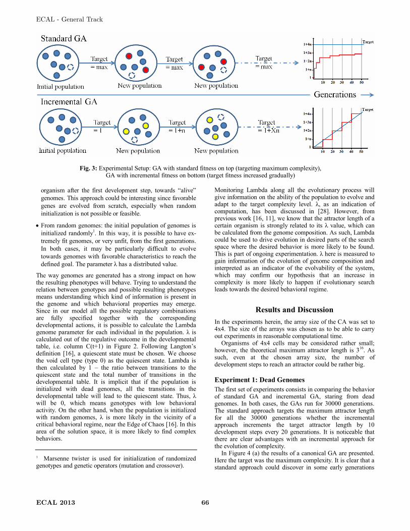
organism after the first development step, towards “alive” genomes. This approach could be interesting since favorable genes are evolved from scratch, especially when random initialization is not possible or feasible.
From random genomes: the initial population of genomes is initialized randomly1. In this way, it is possible to have ex-tremely fit genomes, or very unfit, from the first generations. In both cases, it may be particularly difficult to evolve towards genomes with favorable characteristics to reach the defined goal. The parameter λ has a distributed value.
The way genomes are generated has a strong impact on how the resulting phenotypes will behave. Trying to understand the relation between genotypes and possible resulting phenotypes means understanding which kind of information is present in the genome and which behavioral properties may emerge. Since in our model all the possible regulatory combinations are fully specified together with the corresponding developmental actions, it is possible to calculate the Lambda genome parameter for each individual in the population. λ is calculated out of the regulative outcome in the developmental table, i.e. column C(t+1) in Figure 2. Following Langton’s definition [16], a quiescent state must be chosen. We choose the void cell type (type 0) as the quiescent state. Lambda is then calculated by 1 – the ratio between transitions to the quiescent state and the total number of transitions in the developmental table. It is implicit that if the population is initialized with dead genomes, all the transitions in the developmental table will lead to the quiescent state. Thus, λ will be 0, which means genotypes with low behavioral activity. On the other hand, when the population is initialized with random genomes, λ is more likely in the vicinity of a critical behavioral regime, near the Edge of Chaos [16]. In this area of the solution space, it is more likely to find complex behaviors. 1 Marsenne twister is used for initialization of randomized genotypes and genetic operators (mutation and crossover).
Monitoring Lambda along all the evolutionary process will give information on the ability of the population to evolve and adapt to the target complexity level. λ, as an indication of computation, has been discussed in [28]. However, from previous work [16, 11], we know that the attractor length of a certain organism is strongly related to its λ value, which can be calculated from the genome composition. As such, Lambda could be used to drive evolution in desired parts of the search space where the desired behavior is more likely to be found. This is part of ongoing experimentation. λ here is measured to gain information of the evolution of genome composition and interpreted as an indicator of the evolvability of the system, which may confirm our hypothesis that an increase in complexity is more likely to happen if evolutionary search leads towards the desired behavioral regime.
Results and Discussion In the experiments herein, the array size of the CA was set to 4x4. The size of the arrays was chosen as to be able to carry out experiments in reasonable computational time. Organisms of 4x4 cells may be considered rather small; however, the theoretical maximum attractor length is 316. As such, even at the chosen array size, the number of development steps to reach an attractor could be rather big.
Experiment 1: Dead Genomes The first set of experiments consists in comparing the behavior of standard GA and incremental GA, staring from dead genomes. In both cases, the GAs run for 30000 generations. The standard approach targets the maximum attractor length for all the 30000 generations whether the incremental approach increments the target attractor length by 10 development steps every 20 generations. It is noticeable that there are clear advantages with an incremental approach for the evolution of complexity. In Figure 4 (a) the results of a canonical GA are presented. Here the target was the maximum complexity. It is clear that a standard approach could discover in some early generations
Fig. 3: Experimental Setup: GA with standard fitness on top (targeting maximum complexity), GA with incremental fitness on bottom (target fitness increased gradually)
ECAL - General Track
ECAL 2013 66
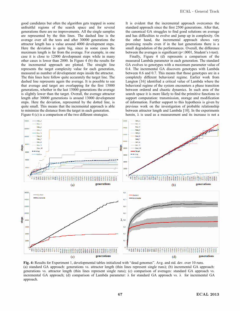
good candidates but often the algorithm gets trapped in some unfruitful regions of the search space and for several generations there are no improvements. All the single samples are represented by the thin lines. The dashed line is the average over all the tests and after 30000 generations the attractor length has a value around 4000 development steps. Here the deviation is quite big, since in some cases the maximum length is far from the average. For example, in one case it is close to 12000 development steps while in many other cases is lower than 2000. In Figure 4 (b) the results for the incremental approach are plotted. The straight line represents the target complexity value for each generation, measured as number of development steps inside the attractor. The thin lines here follow quite accurately the target line. The dashed line represents again the average. It is possible to see that average and target are overlapping for the first 15000 generations, whether in the last 15000 generations the average is slightly lower than the target. Overall, the average attractor length after 30000 generations is around 13000 development steps. Here the deviation, represented by the dotted line, is quite small. This means that the incremental approach is able to minimize the distance from the target in each generation. Figure 4 (c) is a comparison of the two different strategies.
It is evident that the incremental approach overcomes the standard approach since the first 2500 generations. After that, the canonical GA struggles to find good solutions on average and has difficulties to evolve and jump up in complexity. On the other hand, the incremental approach shows very promising results even if in the last generations there is a small degradation of the performances. Overall, the difference between the averages is significant (p<.0001, Student’s t-test). Finally, Figure 4 (d) represents a comparison of the measured Lambda parameter in each generation. The standard GA evolves to genotypes with a maximum parameter value of 0.4. The incremental GA discovers genotypes with Lambda between 0.6 and 0.7. This means that those genotypes are in a completely different behavioral regime. Earlier work from Langton [16] identified a critical value of Lambda where the behavioral regime of the system encounters a phase transition between ordered and chaotic dynamics. In such area of the search space it is more likely to find the primitive functions to support computation: transmission, storage and modification of information. Further support to this hypothesis is given by previous work on the investigation of probable relationship between attractor length and Lambda [10]. In the experiments herein, λ is used as a measurement and its increase is not a
Fig. 4: Results for Experiment 1, developmental tables initialized with “dead genomes”. Avg. and std. dev. over 10 runs. (a) standard GA approach: generations vs. attractor length (thin lines represent single runs); (b) incremental GA approach: generations vs. attractor length (thin lines represent single runs); (c) comparison of averages: standard GA approach vs. incremental GA approach; (d) comparison of Lambda parameter: λ for standard GA approach vs. λ for incremental GA approach.
ECAL - General Track
67 ECAL 2013
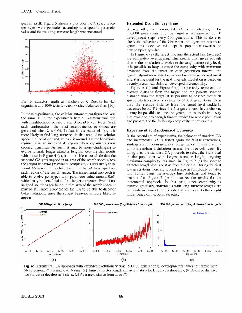
goal in itself. Figure 5 shows a plot over the λ space where genotypes were generated according to a specific parameter value and the resulting attractor length was measured.
Fig. 5: attractor length as function of λ. Results for 4x4 organisms and 1000 tests for each λ value. Adapted from [10]. In those experiments, the cellular automata configuration was the same as in the experiments herein: 2-dimensional grid with neighborhood of size 5 and 3 possible cell types. With such configuration, the most heterogeneous genotypes are generated when λ is 0.66. In fact, in the scattered plot, it is more likely to find long attractors in that area of the solution space. On the other hand, when λ is around 0.4, the behavioral regime is in an intermediate region where organisms show ordered dynamics. As such, it may be more challenging to evolve towards longer attractor lengths. Relating this results with those in Figure 4 (d), it is possible to conclude that the standard GA gets trapped in an area of the search space where the sought behavior (maximum complexity) is less likely to be found. Moreover, it may be difficult for the GA to escape from such region of the search space. The incremental approach is able to evolve genotypes with parameter value around 0,65, which may be beneficial to find longer attractors. Even if not so good solutions are found in that area of the search space, it may be still more probable for the GA to be able to discover better solutions, since the sought behavior is more likely to appear.
Extended Evolutionary Time Subsequently, the incremental GA is executed again for 500.000 generations and the target is incremented by 10 development steps every 500 generations. This is done to check the behavior of the GA when the algorithm has more generations to evolve and adapt the population towards the new complexity value. In Figure 6 (a) the target line and the actual line (average) are completely overlapping. This means that, given enough time to the population to evolve to the sought complexity level, it is possible to keep increase the complexity with minimum deviation from the target. In each generation interval, the genetic algorithm is able to discover favorable genes and use it as a starting point for the next intervals. Evolution is based on already present capabilities, developed incrementally. Figure 6 (b) and Figure 6 (c) respectively represent the average distance from the target and the percent average distance from the target. It is possible to observe that such span predictably increases along the 500000 generations. Even that, the average distance from the target level suddenly decreases below 1% since the first generations. In conclusion, it may be possible to tune the generation intervals in a way that evolution has enough time to evolve the whole population and prepare it to the following complexity improvements.
Experiment 2: Randomized Genomes In the second set of experiments, the behavior of standard GA and incremental GA is tested again for 50000 generations, starting from random genomes, i.e. genomes initialized with a uniform random distribution among the three cell types. By doing that, the standard GA proceeds to select the individual in the population with longest attractor length, targeting maximum complexity. As such, in Figure 7 (a) the average attractor length does not start from the origin. During the first few generations there are several jumps in complexity but after this fruitful stage the average line stabilizes and tends to become flat. Figure 7 (b) summarizes the results for the incremental approach. In this case, since complexity is evolved gradually, individuals with long attractor lengths are left aside in favor of individuals that are closer to the sought initial behavior, i.e. point attractor.
Fig. 6: Incremental GA approach with extended evolutionary time (500000 generations), developmental tables initialized with “dead genomes”, average over 6 runs. (a) Target attractor length and actual attractor length (overlapping); (b) Average distance from target in development steps; (c) Average distance from target %
ECAL - General Track
ECAL 2013 68
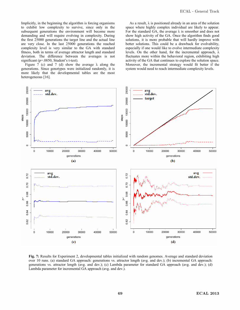
Implicitly, in the beginning the algorithm is forcing organisms to exhibit low complexity to survive, since only in the subsequent generations the environment will become more demanding and will require evolving in complexity. During the first 25000 generations the target line and the actual line are very close. In the last 25000 generations the reached complexity level is very similar to the GA with standard fitness, both in terms of average attractor length and standard deviation. The difference between the averages is not significant (p=.0850, Student’s t-test). Figure 7 (c) and 7 (d) show the average λ along the generations. Since genotypes were initialized randomly, it is more likely that the developmental tables are the most heterogeneous [16].
As a result, λ is positioned already in an area of the solution space where highly complex individual are likely to appear. For the standard GA, the average λ is smoother and does not show high activity of the GA. Once the algorithm finds good solutions, it is more probable that will hardly improve with better solutions. This could be a drawback for evolvability, especially if one would like to evolve intermediate complexity levels. On the other hand, for the incremental approach, λ fluctuates more within the behavioral region, exhibiting high activity of the GA that continues to explore the solution space. Moreover, the incremental strategy would fit better if the system would need to reach intermediate complexity levels.
Fig. 7: Results for Experiment 2, developmental tables initialized with random genomes. Average and standard deviation over 10 runs. (a) standard GA approach: generations vs. attractor length (avg. and dev.); (b) incremental GA approach: generations vs. attractor length (avg. and dev.); (c) Lambda parameter for standard GA approach (avg. and dev.); (d) Lambda parameter for incremental GA approach (avg. and dev.).
ECAL - General Track
69 ECAL 2013
Conclusion The presented experiments investigated the emergence of complexity in cellular machines, using two different evolutionary strategies: a standard approach, where the target was the maximum complexity and an incremental approach, where complexity was gradually evolved. We showed that the incremental approach has clear advantages when evolution targets an increase of complexity, especially when the population’s genome parameter is towards uniform, i.e. intermediate complexity levels in equilibrium with the environmental pressure. Such knowledge is important at the design stage of EvoDevo systems, where developmental actions are not manually programmed but discovered through evolutionary processes.
We also proposed the usage of Lambda genome parameter to detect the behavioral regime. This may be useful to indicate if the evolving genomes are likely to be able to achieve more complex behaviors, giving information on the evolvability of the system. Such ability of adaptive evolution is necessary for a system to be able to evolve complexity. Moreover, when it comes to adaptivity, the results herein show that genomes with a given parameter value will most likely mutate to genomes with similar developmental behavior, as long as the mutation results in an offspring with similar parameter value. Our current work is focused on the usage of genome parameters to guide evolution towards favorable areas of the solution space. Furthermore, genome parameters may help to keep the population closer to the desired developmental behavior and supervising its genetic distance. This is in tune with at least two points of the current challenges in the field of artificial life [4]: “explain how rules and symbols are generated from physical dynamics” and “develop a theory of information processing, information flow and information generation for evolving systems”.
As a future work, it may be possible to compare the robustness of solutions evolved incrementally versus solutions evolved with a standard approach. In particular, how fragile they are to external perturbation, both at genotype level, i.e. mutations in the rule table, and at phenotype level, i.e. perturbation of the system state during development.
References [1] F. Gomez and R. Miikkulainen. Incremental evolution of complex
general behavior. Adaptive Behavior, 5: pages 317-342 (1997). [2] M. Schuster and C. Harman. Incremental evolution of complex light
switching behavior. CS 81 Adaptive Robotics. Swarthmore College (2006).
[3] K. O. Stanley and R. Miikkulainen. Competitive coevolution through evolutionary complexification. Journal of artificial intelligence research, 21: pages 63-100 (2004).
[4] M. Bedau, J. McCaskill, N. Packard, S. Rasmussen, C. Adami, D. Green, T. Ikegami, K. Kaneko and T. Ray. Open problems in artificial life. Artificial Life, 6: pages 363-373 (2000).
[5] T. Kowaliw. Measures of complexity for artificial embryogeny. GECCO 2008, pages 843-850. ACM (2008)
[6] P. K. Lehre and P. C. Haddow. Developmental mappings and phenotypic complexity. In Congress on Evolutionary Computation, CEC2003, pages 62–68. IEEE (2003).
[7] R. Doursat, H. Sayama and O. Michel. Morphogenetic engineering: toward programmable complex systems. Understanding Complex Systems Series, Springer-Verlag (2012).
[8] R. Doursat, C. Sánchez, R. Dordea, D. Fourquet and T. Kowaliw. Embryomorphic engineering: emergent innovation through evolutionary development. In Morphogenetic Engineering: Toward Programmable Complex Systems, R. Doursat, H. Sayama and O. Michel, pages 275-311. "Understanding Complex Systems" Series, Springer-Verlag (2012).
[9] S. Harding and W. Banzhaf. Organic Computing, chapter Artificial Development, pages 201–220. Springer Verlag (2008).
[10] G. Tufte and S. Nichele. On the correlations between developmental diversity and genomic composition. 13th Annual Genetic and Evolutionary Computation Conference, GECCO 2011, pages 1507-1514. ACM (2011).
[11] S. Nichele and G. Tufte. Genome parameters as information to forecast emergent developmental behaviors. 11th International Conference on Unconventional Computation and Natural Computation, UCNC 2012, pages 186-197. Springer (2012).
[12] D. Floreano and S. Nolfi. God save the red queen! Competition in co-evolutionary robotics. Evolutionary computation, 5 (1997).
[13] S. Wolfram. Universality and complexity in CA. Physica D, 10 (1-2): pages 1–35 (1984).
[14] M. Kirschner and J. Gerhart. The plausibility of life: resolving Darwin’s dilemma. Yale University press (2006).
[15] U. Krohs and O. Kroes. Functions in biological and artificial worlds. The Vienna series in theoretical biology. MIT press (2009).
[16] C. G. Langton. Computation at the edge of chaos: phase transitions and emergent computation. In S. Forrest, editor, Emergent Computation, pages 12–37. MIT Press (1991).
[17] C. G. Langton: Self-reproduction in cellular automata. Physica D, 10: pages 135–144 (1984).
[18] M. J. West-Eberhard. Developmental plasticity and evolution. Oxford Univ. Press (2003).
[19] G. Tufte. Evolution, development and environment toward adaptation through phenotypic plasticity and exploitation of external information. S. Bullock, J. Noble, R. Watson, and M. A. Bedau, editors, Artificial Life XI, pages 624–631. MIT Press, Cambridge, MA (2008).
[20] G. de Oliveira, P. de Oliveira and N. Omar. Definition and application of a five-parameter characterization of one-dimensional cellular automata rule space. MIT, Artificial Life7: pages 277-301 (2001).
[21] W. Li. Phenomenology of nonlocal cellular automata. Santa Fe Institute. Journal of Statistical Physics, 68(5-6): pages 829-882 (1992).
[22] P. M. Binder. A phase diagram for elementary cellular automata. Complex Systems, 7, pages 241-247 (1993).
[23] P. M. Binder. Parametric ordering of complex systems. Physical Review E, vol. 49 n. 3, pages 2023-2025 (1994).
[24] G. de Oliveira, P. de Oliveira and N. Omar. Guidelines for dynamics-based parameterization of one-dimensional cellular automata rule space. John Wiley & Sons, Inc. Vol. 6, No. 2 Complexity (2001).
[25] T. Kowaliw, P. Grogono and N. Kharma. Environment as a spatial constraint on the growth of structural form. GECCO 2007, pages 1037–1044, New York, NY, USA (2007).
[26] J. F. Miller and W. Banzhaf. Evolving the program for a cell: from french flag to boolean circuits. In S. Kumar and P. J. Bentley, editors, On Growth, Form and Computers, pages 278–301. Elsevier Limited Oxford UK (2003).
[27] R. Dawkins. The blind watchmaker. Chapter 3: accumulating small changes. Norton & Company Inc. (1986).
[28] M. Mitchell, P. T. Hraber and J. P. Crutchfield. Revisiting the Edge of Chaos: evolving cellular automata to perform computations. Complex Systems 7: pages 89-130 (1993).
ECAL - General Track
ECAL 2013 70
Paper C.2
Investigation of Genome Parameters and Sub-Transitions
to Guide Evolution of Artificial Cellular Organisms
S. Nichele, H. Wold and G. Tufte
16th European Conference on the Applications of Evolutionary Computation,
EvoApplications 2014
April 23 - 25, 2014
Granada, Spain

100
© Springer-Verlag Berlin Heidelberg 2014 A.I. Esparcia-Alcázar et al. (Eds.): EvoApplications 2014, LNCS 8602, pp. 113–124, 2014. DOI: 10.1007/978-3-662-45523-4_10
Investigation of Genome Parameters and Sub-transitions to Guide Evolution of Artificial Cellular Organisms
Stefano Nichele(), Håkon Hjelde Wold, and Gunnar Tufte
Department of Computer and Information Science, Norwegian University of Science and Technology,
Sem Selandsvei 7-9, 7491, Trondheim, Norway {nichele,gunnart}@idi.ntnu.no, [email protected]
Abstract. Artificial multi-cellular organisms develop from a single zygote to complex morphologies, following the instructions encoded in their genomes. Small genome mutations can result in very different developed phenotypes. In this paper we investigate how to exploit genotype information in order to guide evolution towards favorable areas of the phenotype solution space, where the sought emergent behavior is more likely to be found. Lambda genome parame-ter, with its ability to discriminate different developmental behaviors, is incor-porated into the fitness function and used as a discriminating factor for genetic distance, to keep resulting phenotype’s developmental behavior close by and encourage beneficial mutations that yield adaptive evolution. Genome activa-tion patterns are detected and grouped into genome parameter sub-transitions. Different sub-transitions are investigated as simple genome parameters, or composed to integrate several genome properties into a more exhaustive com-posite parameter. The experimental model used herein is based on 2-dimensional cellular automata.
Keywords: Artificial Development · Evolution · Complexity · Emergence · Cellular Automata
1 Introduction
Evolved artificial developmental (EvoDevo) systems have shown many favorable features that are also present in natural biological systems, such as the ability to evolve robust genomes [1]. However, robustness and evolvability may not be always rowing in the same direction. A biological organism may be considered robust if, after genome mutations, it keeps the same ability or functional properties. In contrast, evolvability is a property that promotes genetic variation in order to produce adaptive evolution, being able to evolve through natural selection. One may think that too high robustness would not provide enough genetic diversity whereas too high evolvability would cause more disadvantageous mutations, thus annihilating adaptation. In EvoDevo systems, small changes in the genome often lead to completely different emergent phenotypes. It is particularly difficult to understand which changes will be produced to the developing organism by each genetic operator, e.g. mutation, crosso-ver, and which phenotypic traits will be affected. As such, evolutionary algorithms
114 S. Nichele et al.
spend a relevant amount of time generating low fitness solutions that may not give any genetic contribution to the population and thus being often discarded. We investi-gate if genome information could be used to guide evolution. Our results indicate that genome parameters could predict the developing behavior based on genome composi-tion and thus help to guide evolutionary search in the right area of the search space, where the sought behavior is more likely to be found.
The article is laid out as follows: background information and motivation is pre-sented in Section 2. In Section 3 the developmental model used in the experiments is presented. Section 4 describes Lambda genome parameter, meaning and usage. The experimental setup is illustrated in Section 5. In Section 6 and 7 the results of the experiments are presented together with the discussion. Section 8 concludes the work.
2 Motivation and Background
Artificial developmental systems can be considered as complex systems [2], where there is no central controller and the developed artificial organisms are the result of an emergent process out of the local interactions of simple cells. Many developmental systems target specific phenotypic structures or structural properties [3], whether some others execute a particular computational task that emerges out of the develop-ment of the machine’ structure [4]. Programming an artificial developmental system to produce such emergent computation cannot be done using traditional engineering approaches. One solution could be to exploit nature’s way of tackling problems, namely evolution by natural selection. Evolutionary algorithms have been widely used as population-based metaheuristic optimization algorithms [5]. In general, those evolutionary techniques do not make any assumption about the underlying fitness landscape. An indirect genotype-to-phenotype mapping can result in two very similar genotypes developing into two very different phenotypes. A developmental mapping may be represented by a function that maps elements in the genotype space to ele-ments in the phenotype space. Such spaces may have regions where small distances between genotypes are preserved into small differences between resulting phenotypes, whether in some other regions distances are hardly preserved at all [12]. In practice, small mutation can have a huge impact on the emergent phenotype. This can be problematic if solutions are to be discovered by evolutionary algorithms. Having a genome parameter that may predict the emergent behavior could be useful to reduce phenotypic distance. Such information could contribute to guide evolutionary search throughout the solution space, where the target phenotype may plausibly appear.
3 Evolution and Development
The relation between natural evolution and development in biological systems is still a fairly unexplored area [13]. Investigation of natural evolution makes it hardly possible to obtain experimental proofs due to the time scale of evolution. In evolved artificial systems there is no such problem. It is possible to execute experiments in a reasonable time and investigate different evolutionary factors that may influence on developmental paths. However, there is a lack of knowledge of what kind of information must be
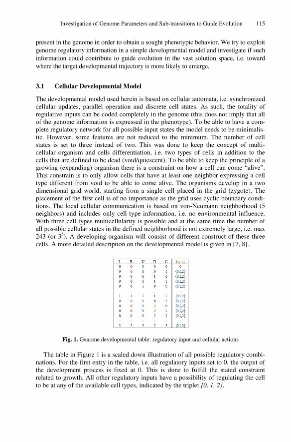
Investigation of Genome Parameters and Sub-transitions to Guide Evolution 115
present in the genome in order to obtain a sought phenotypic behavior. We try to exploit genome regulatory information in a simple developmental model and investigate if such information could contribute to guide evolution in the vast solution space, i.e. toward where the target developmental trajectory is more likely to emerge.
3.1 Cellular Developmental Model
The developmental model used herein is based on cellular automata, i.e. synchronized cellular updates, parallel operation and discrete cell states. As such, the totality of regulative inputs can be coded completely in the genome (this does not imply that all of the genome information is expressed in the phenotype). To be able to have a com-plete regulatory network for all possible input states the model needs to be minimalis-tic. However, some features are not reduced to the minimum. The number of cell states is set to three instead of two. This was done to keep the concept of multi-cellular organism and cells differentiation, i.e. two types of cells in addition to the cells that are defined to be dead (void/quiescent). To be able to keep the principle of a growing (expanding) organism there is a constraint on how a cell can come “alive”. This constrain is to only allow cells that have at least one neighbor expressing a cell type different from void to be able to come alive. The organisms develop in a two dimensional grid world, starting from a single cell placed in the grid (zygote). The placement of the first cell is of no importance as the grid uses cyclic boundary condi-tions. The local cellular communication is based on von-Neumann neighborhood (5 neighbors) and includes only cell type information, i.e. no environmental influence. With three cell types multicellularity is possible and at the same time the number of all possible cellular states in the defined neighborhood is not extremely large, i.e. max 243 (or 35). A developing organism will consist of different construct of these three cells. A more detailed description on the developmental model is given in [7, 8].
Fig. 1. Genome developmental table: regulatory input and cellular actions
The table in Figure 1 is a scaled down illustration of all possible regulatory combi-nations. For the first entry in the table, i.e. all regulatory inputs set to 0, the output of the development process is fixed at 0. This is done to fulfill the stated constraint related to growth. All other regulatory inputs have a possibility of regulating the cell to be at any of the available cell types, indicated by the triplet {0, 1, 2}.
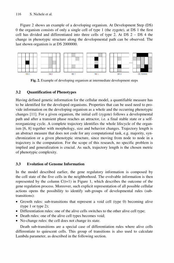
116 S. Nichele et al.
Figure 2 shows an exam0 the organism consists of cell has divided and differchange in phenotypic struclast shown organism is at D
Fig. 2. Example of d
3.2 Quantification of P
Having defined genetic infoto be identified for the devevide information on the devchanges [11]. For a given opath and after a transient preorganizing cycle. A compism [6, 8] together with moan abstract measure that dochronization or a given phtrajectory is the computatioimplied and generalization of phenotypic complexity.
3.3 Evolution of Genom
In the model described ethe cell state of the five celrepresented by the columngene regulation process. Moactions opens the possibiltransitions):
• Growth rules: sub-trans(type 1 or type 2);
• Differentiation rules: one• Death rules: one of the a• No-change rules: the cell
Death sub-transitions ardifferentiate to quiescent cLambda parameter, as descr
mple of a developing organism. At Development Step (Donly a single cell of type 1 (the zygote), at DS 1 the f
rentiated into three cells of type 2. At DS 2 – DS 4 cture along the developmental path can be observed. T
DS 2000000.
developing organism at intermediate development steps
Phenotypes
ormation for the cellular model, a quantifiable measure eloped organisms. Properties that can be used need to pveloping organism as a whole and the occurring phenotyorganism, the initial cell (zygote) follows a developmen
phase reaches an attractor, i.e. a final stable state or a splete trajectory identifies the whole lifecycle of the orgorphology, size and behavior changes. Trajectory lengthoes not code for any computational task, e.g. majority, shenotypic structure, since moving from node to node ion. For the scope of this research, no specific problemis crucial. As such, trajectory length is the chosen me
me Information
arlier, the gene regulatory information is composed lls in the neighborhood. The evolvable information is t
n C(t+1) in Figure 1, which describes the outcome of oreover, such explicit representation of all possible cellulity to identify sub-groups of developmental rules (s
itions that represent a void cell (type 0) becoming al
e of the alive cells switches to the other alive cell type; live cell types becomes void; l does not change its state.
re a special case of differentiation rules where alive ccells. This group of transitions is also used to calcuribed in the following section.
DS) first the
The
has pro-ypic ntal
self-gan-h is
syn-in a m is etric
by then the
ular sub-
live
cells late
Investigation of Genome Parameters and Sub-transitions to Guide Evolution 117
The developmental trajectory from zygote to multi-cellular organism can be repre-sented by the state transition in Figure 2. Such trajectory produces a genome activa-tion pattern at each development step that can be measured in terms of sub-transitions activated in the genome. For example, from DS 0 to DS 1 only one differentiation sub-transition is activated, together with three growth sub-transitions and twenty one no-change sub-transitions. No death sub-transitions are triggered.
4 Lambda Genome Parameter
Parameters obtained from the genome information can be used to estimate the dynamic developmental behavior of the emerging organisms. Langton [6] tried to find a relation between CA behavior and a parameter λ. He observed that the basic functions required for computation (transmission, storage and modification of information) are more likely to be achieved in the vicinity of phase transitions between ordered and disordered dy-namics (edge of chaos). He hypothesized that it is easier to find rules capable of complex computation in a region where the value of λ is critical. Since the developmental model is composed by 35 regulatory combinations, all the possible regulatory inputs and relative outputs (growth, differentiation, death or no action) are fully specified in the develop-mental table. In order to calculate λ, it is necessary to define a quiescent state, the void cell (type 0) in our case. Lambda is defined as follows:
(1)
λ can be calculated according to Equation 1, where n represents the number of transitions to the quiescent (dead) state, K is the number of cells types (three in our case) and N is the neighborhood size (five in the Von Neumann neighborhood). In this way, the value of λ is based only on local properties of the neighborhood and in particular the cellular actions that are present in every cell.
Previous works [6, 7] have shown a clear relation between Lambda parameter and developed organisms’ trajectory length. In particular, it is possible to identify a pa-rameter space interval where organisms are more likely to have long life cycles. As such, Lambda (or other genome parameters) could be used to guide evolution when the target fitness is based on organisms’ developing trajectories, as the work herein.
As shown in Equation 1, Lambda is determined by the ratio of sub-transitions in the developmental table that lead to the quiescent state over the total number of sub-transitions in the regulatory table. As such, λ takes into account only developmental rules that describe a cell death, i.e. one of the alive cell types becomes void. In other words, it does not consider other sub-transition groups (growth, differentiation, no-change). Lambda can be considered a single sub-transition genome parameter.
4.1 Genome Parameter Sub-transitions
Lambda parameter has been shown to be able to differentiate different developmental behaviors (transient, attractor and trajectory length) for boolean CAs [6, 9, 10] and
118 S. Nichele et al.
with organisms with 3 cell types [7, 8]. When the number of possible cell states gets bigger, Lambda may not be able to capture genome properties related to transitions to the chosen quiescent states. This is due to the presence of a growing number of sub-transition classes. Lambda’s meaning would then be loose and be interpreted just as one of the many sub-transition classes in the genome table. On the other hand, there exist many sub-transitions parameters that hold the same parameter distribution as Lambda. Such sub-transition parameters could be then composed to create a custom parameter that captures the same genome properties as Lambda does.
5 Experimental Setup
In the experiment herein the presented developmental model with organism size of 4x4 cells is used. This leads to a theoretical maximum trajectory length and attractor length of 316 development steps.
The genetic algorithm uses a population of 24 genotypes with elitism. The 8 worst individuals are replaced in each generation by newly generated offspring, selected through proportionate selection. Each two selected genotypes undergo one-point uni-form crossover with probability 0.7 and mutation with probability 0.02 per gene. The genotype initial population is initialized with void genomes, i.e. all the transitions in the developmental table lead to the quiescent state. This means that the resulting phe-notypes are the most unfit and difficult to evolve, i.e. dead organisms that end-up in a point attractor after a single development step. This is done to provide an even start-ing point for comparison.
In the standard GA (used as reference), the fitness is proportional to the developed trajectory length (the longer the fitter). In the GA that uses Lambda genome parame-ter contribution in the fitness function, the combined fitness (CFitness) is calculated as follows:
(2)
In Equation 2, the used ratio is 0.2 (1) and HiLambda represents the Lambda value where the longest trajectory length is more likely to be found (0.66 in our model), i.e. critical Lambda [6].
6 Genome Parameter to Guide Evolution
In this first experiment, performances of a conventional genetic algorithm are com-pared to a GA that encapsulates Lambda in the fitness function. The chosen trajectory length targets are set as 1000, 5000, 10000 and 15000 development steps (average over 1000 runs for target 1000, average over 20 runs for the other targets due to runtime). Results are shown in Figures from 3 to 6 respectively. In all the four consid-ered cases, the effect of Lambda in fitness is clearly visible. 1 The ratio that gave best results for GA with λ in fitness from randomized genomes is 0.05.
Otherwise 0.2 is used in all the plotted results.
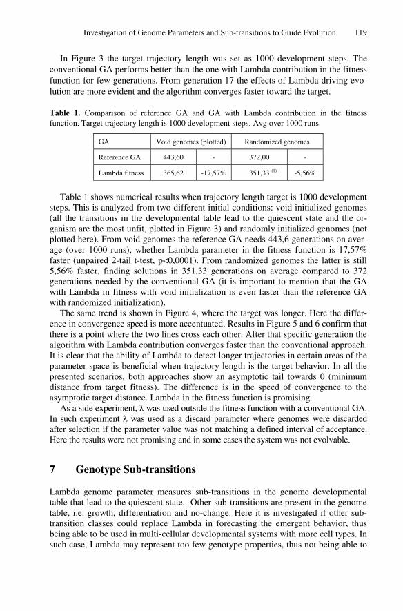
Investigation of Genome Parameters and Sub-transitions to Guide Evolution 119
In Figure 3 the target trajectory length was set as 1000 development steps. The conventional GA performs better than the one with Lambda contribution in the fitness function for few generations. From generation 17 the effects of Lambda driving evo-lution are more evident and the algorithm converges faster toward the target.
Table 1. Comparison of reference GA and GA with Lambda contribution in the fitness function. Target trajectory length is 1000 development steps. Avg over 1000 runs.
GA Void genomes (plotted) Randomized genomes
Reference GA 443,60 - 372,00 -
Lambda fitness 365,62 -17,57% 351,33 (1) -5,56%
Table 1 shows numerical results when trajectory length target is 1000 development
steps. This is analyzed from two different initial conditions: void initialized genomes (all the transitions in the developmental table lead to the quiescent state and the or-ganism are the most unfit, plotted in Figure 3) and randomly initialized genomes (not plotted here). From void genomes the reference GA needs 443,6 generations on aver-age (over 1000 runs), whether Lambda parameter in the fitness function is 17,57% faster (unpaired 2-tail t-test, p<0,0001). From randomized genomes the latter is still 5,56% faster, finding solutions in 351,33 generations on average compared to 372 generations needed by the conventional GA (it is important to mention that the GA with Lambda in fitness with void initialization is even faster than the reference GA with randomized initialization).
The same trend is shown in Figure 4, where the target was longer. Here the differ-ence in convergence speed is more accentuated. Results in Figure 5 and 6 confirm that there is a point where the two lines cross each other. After that specific generation the algorithm with Lambda contribution converges faster than the conventional approach. It is clear that the ability of Lambda to detect longer trajectories in certain areas of the parameter space is beneficial when trajectory length is the target behavior. In all the presented scenarios, both approaches show an asymptotic tail towards 0 (minimum distance from target fitness). The difference is in the speed of convergence to the asymptotic target distance. Lambda in the fitness function is promising.
As a side experiment, λ was used outside the fitness function with a conventional GA. In such experiment λ was used as a discard parameter where genomes were discarded after selection if the parameter value was not matching a defined interval of acceptance. Here the results were not promising and in some cases the system was not evolvable.
7 Genotype Sub-transitions
Lambda genome parameter measures sub-transitions in the genome developmental table that lead to the quiescent state. Other sub-transitions are present in the genome table, i.e. growth, differentiation and no-change. Here it is investigated if other sub-transition classes could replace Lambda in forecasting the emergent behavior, thus being able to be used in multi-cellular developmental systems with more cell types. In such case, Lambda may represent too few genotype properties, thus not being able to
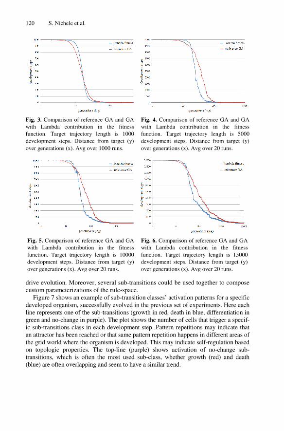
120 S. Nichele et al.
Fig. 3. Comparison of referenwith Lambda contribution function. Target trajectory ldevelopment steps. Distance over generations (x). Avg over
Fig. 5. Comparison of referenwith Lambda contribution function. Target trajectory ldevelopment steps. Distance over generations (x). Avg ove
drive evolution. Moreover, custom parameterizations o
Figure 7 shows an exampdeveloped organism, succesline represents one of the sugreen and no-change in purpic sub-transitions class in eaan attractor has been reachedthe grid world where the orgon topologic properties. Ttransitions, which is often (blue) are often overlapping
nce GA and GA
in the fitness length is 1000 from target (y)
r 1000 runs.
Fig. 4. Comparison of reference GA and with Lambda contribution in the fitnfunction. Target trajectory length is 5development steps. Distance from target over generations (x). Avg over 20 runs.
nce GA and GA
in the fitness ength is 10000 from target (y)
er 20 runs.
Fig. 6. Comparison of reference GA and Gwith Lambda contribution in the fitnfunction. Target trajectory length is 150development steps. Distance from target over generations (x). Avg over 20 runs.
several sub-transitions could be used together to compof the rule-space. ple of sub-transition classes’ activation patterns for a specssfully evolved in the previous set of experiments. Here eub-transitions (growth in red, death in blue, differentiationple). The plot shows the number of cells that trigger a speach development step. Pattern repetitions may indicate d or that same pattern repetition happens in different areaganism is developed. This may indicate self-regulation ba
The top-line (purple) shows activation of no-change sthe most used sub-class, whether growth (red) and deand seem to have a similar trend.
GA
ness 5000
(y)
GA
ness 000 (y)
pose
cific each n in
ecif-that
as of ased sub-eath
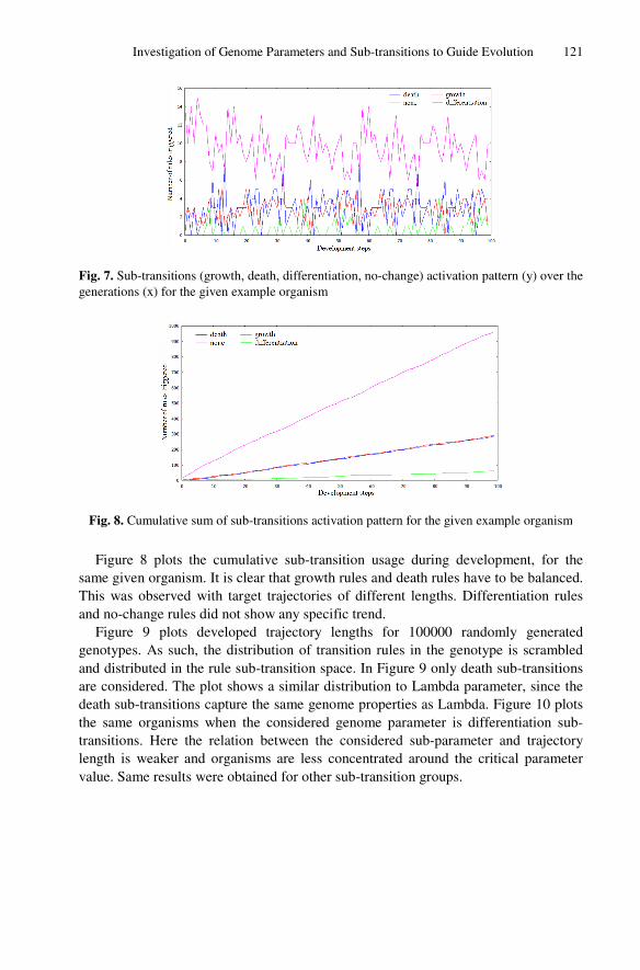
Investigation of Gen
Fig. 7. Sub-transitions (growthgenerations (x) for the given ex
Fig. 8. Cumulative sum of su
Figure 8 plots the cumsame given organism. It is cThis was observed with taand no-change rules did not
Figure 9 plots developgenotypes. As such, the diand distributed in the rule sare considered. The plot shdeath sub-transitions capturthe same organisms when transitions. Here the relatilength is weaker and organvalue. Same results were ob
nome Parameters and Sub-transitions to Guide Evolution
h, death, differentiation, no-change) activation pattern (y) overxample organism
ub-transitions activation pattern for the given example organis
mulative sub-transition usage during development, for clear that growth rules and death rules have to be balanc
arget trajectories of different lengths. Differentiation rut show any specific trend. ped trajectory lengths for 100000 randomly generastribution of transition rules in the genotype is scrambsub-transition space. In Figure 9 only death sub-transitihows a similar distribution to Lambda parameter, since re the same genome properties as Lambda. Figure 10 pthe considered genome parameter is differentiation s
ion between the considered sub-parameter and trajectnisms are less concentrated around the critical paramebtained for other sub-transition groups.
121
r the
sm
the ced. ules
ated bled ions the
plots sub-tory eter
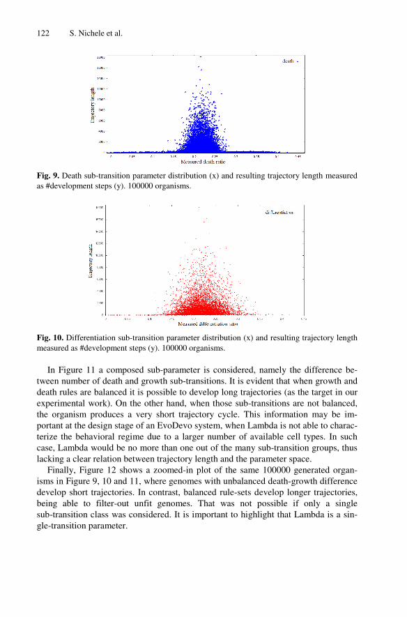
122 S. Nichele et al.
Fig. 9. Death sub-transition paas #development steps (y). 100
Fig. 10. Differentiation sub-trameasured as #development ste
In Figure 11 a composetween number of death anddeath rules are balanced it iexperimental work). On thethe organism produces a vportant at the design stage oterize the behavioral regimcase, Lambda would be no lacking a clear relation betw
Finally, Figure 12 showisms in Figure 9, 10 and 11develop short trajectories. Ibeing able to filter-out usub-transition class was congle-transition parameter.
arameter distribution (x) and resulting trajectory length measu0000 organisms.
ansition parameter distribution (x) and resulting trajectory leneps (y). 100000 organisms.
ed sub-parameter is considered, namely the difference d growth sub-transitions. It is evident that when growth is possible to develop long trajectories (as the target in e other hand, when those sub-transitions are not balancvery short trajectory cycle. This information may be of an EvoDevo system, when Lambda is not able to char
me due to a larger number of available cell types. In smore than one out of the many sub-transition groups, t
ween trajectory length and the parameter space. ws a zoomed-in plot of the same 100000 generated org
, where genomes with unbalanced death-growth differeIn contrast, balanced rule-sets develop longer trajector
unfit genomes. That was not possible if only a sinnsidered. It is important to highlight that Lambda is a
ured
ngth
be-and our
ced, im-rac-uch thus
gan-ence ries, ngle sin-
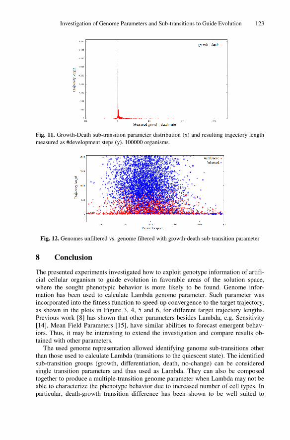
Investigation of Gen
Fig. 11. Growth-Death sub-trameasured as #development ste
Fig. 12. Genomes unfiltered
8 Conclusion
The presented experiments cial cellular organism to gwhere the sought phenotypmation has been used to cincorporated into the fitnessas shown in the plots in FiPrevious work [8] has show[14], Mean Field Parameteiors. Thus, it may be interetained with other parameter
The used genome represthan those used to calculatesub-transition groups (growsingle transition parametertogether to produce a multipable to characterize the pheparticular, death-growth tr
nome Parameters and Sub-transitions to Guide Evolution
ansition parameter distribution (x) and resulting trajectory leneps (y). 100000 organisms.
vs. genome filtered with growth-death sub-transition paramet
investigated how to exploit genotype information of artguide evolution in favorable areas of the solution spapic behavior is more likely to be found. Genome infalculate Lambda genome parameter. Such parameter ws function to speed-up convergence to the target trajectoigure 3, 4, 5 and 6, for different target trajectory lengwn that other parameters besides Lambda, e.g. Sensitiv
ers [15], have similar abilities to forecast emergent behesting to extend the investigation and compare results rs. sentation allowed identifying genome sub-transitions ote Lambda (transitions to the quiescent state). The identifwth, differentiation, death, no-change) can be consides and thus used as Lambda. They can also be compople-transition genome parameter when Lambda may notenotype behavior due to increased number of cell typesansition difference has been shown to be well suited
123
ngth
ter
tifi-ace, for-was ory,
gths. vity hav-ob-
ther fied ered osed t be
s. In d to
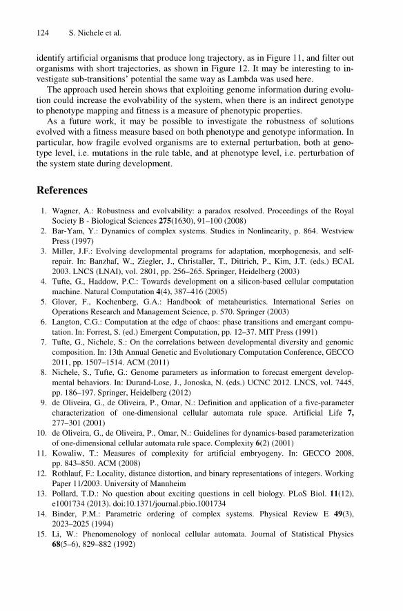
124 S. Nichele et al.
identify artificial organisms that produce long trajectory, as in Figure 11, and filter out organisms with short trajectories, as shown in Figure 12. It may be interesting to in-vestigate sub-transitions’ potential the same way as Lambda was used here.
The approach used herein shows that exploiting genome information during evolu-tion could increase the evolvability of the system, when there is an indirect genotype to phenotype mapping and fitness is a measure of phenotypic properties.
As a future work, it may be possible to investigate the robustness of solutions evolved with a fitness measure based on both phenotype and genotype information. In particular, how fragile evolved organisms are to external perturbation, both at geno-type level, i.e. mutations in the rule table, and at phenotype level, i.e. perturbation of the system state during development.
References
1. Wagner, A.: Robustness and evolvability: a paradox resolved. Proceedings of the Royal Society B - Biological Sciences 275(1630), 91–100 (2008)
2. Bar-Yam, Y.: Dynamics of complex systems. Studies in Nonlinearity, p. 864. Westview Press (1997)
3. Miller, J.F.: Evolving developmental programs for adaptation, morphogenesis, and self-repair. In: Banzhaf, W., Ziegler, J., Christaller, T., Dittrich, P., Kim, J.T. (eds.) ECAL 2003. LNCS (LNAI), vol. 2801, pp. 256–265. Springer, Heidelberg (2003)
4. Tufte, G., Haddow, P.C.: Towards development on a silicon-based cellular computation machine. Natural Computation 4(4), 387–416 (2005)
5. Glover, F., Kochenberg, G.A.: Handbook of metaheuristics. International Series on Operations Research and Management Science, p. 570. Springer (2003)
6. Langton, C.G.: Computation at the edge of chaos: phase transitions and emergant compu-tation. In: Forrest, S. (ed.) Emergent Computation, pp. 12–37. MIT Press (1991)
7. Tufte, G., Nichele, S.: On the correlations between developmental diversity and genomic composition. In: 13th Annual Genetic and Evolutionary Computation Conference, GECCO 2011, pp. 1507–1514. ACM (2011)
8. Nichele, S., Tufte, G.: Genome parameters as information to forecast emergent develop-mental behaviors. In: Durand-Lose, J., Jonoska, N. (eds.) UCNC 2012. LNCS, vol. 7445, pp. 186–197. Springer, Heidelberg (2012)
9. de Oliveira, G., de Oliveira, P., Omar, N.: Definition and application of a five-parameter characterization of one-dimensional cellular automata rule space. Artificial Life 7, 277–301 (2001)
10. de Oliveira, G., de Oliveira, P., Omar, N.: Guidelines for dynamics-based parameterization of one-dimensional cellular automata rule space. Complexity 6(2) (2001)
11. Kowaliw, T.: Measures of complexity for artificial embryogeny. In: GECCO 2008, pp. 843–850. ACM (2008)
12. Rothlauf, F.: Locality, distance distortion, and binary representations of integers. Working Paper 11/2003. University of Mannheim
13. Pollard, T.D.: No question about exciting questions in cell biology. PLoS Biol. 11(12), e1001734 (2013). doi:10.1371/journal.pbio.1001734
14. Binder, P.M.: Parametric ordering of complex systems. Physical Review E 49(3), 2023–2025 (1994)
15. Li, W.: Phenomenology of nonlocal cellular automata. Journal of Statistical Physics 68(5–6), 829–882 (1992)
Paper D.1
Evolutionary Growth of Genome Representations
on Artificial Cellular Organisms with Indirect Encodings
S. Nichele, A. Giskeødegård and G. Tufte
SUBMITTED TO: Artificial Life Journal (MIT Press), Official Journal of the
International Society of Artificial Life

114
Evolutionary Growth of Genome Representations on
Artificial Cellular Organisms with Indirect Encodings
Stefano Nichele *, Andreas Giskeødegård and Gunnar Tufte
Norwegian University of Science and Technology
Department of Computer and Information Science Sem Selandsvei 7-9, 7491, Trondheim, Norway
[email protected], [email protected], [email protected]
* corresponding author
Abstract—Evolutionary design targets systems of continuously increasing complexity and size. Thus,
developmental or generative mappings, i.e. indirect encodings, are often a necessity. “Scaling-up” the complexity of a
developed phenotype, and thus the relative solution space, does not explicitly affect the genotype search space, since
each genotype does not represent a specific phenotype object directly. Phenotype solutions are the result of an
incremental building process. As the phenotype information is not encoded directly into a low-level genotype, the
high-level developing information relies on efficient mapping. Varying the amount of genotype information changes
the cardinality of the mapping which, in turn, affects the development process. This raises several open questions:
How much information must be present in the genotype? How to find the genotype size and representation in which a
developmental solution of given complexity would fit? Using the whole set of possible regulatory combinations may be
intractable or hardly evolvable due to the cardinality of the search space. On the other hand, a restricted pool of genes
may not be large enough to encode a solution, i.e. potential solutions may be excluded due to a reduced solution space,
or may need complex heuristics to find a realistic size. In nature, the genomes of biological organisms are not fixed in
size; they slowly evolve and acquire new genes by random gene duplications. Newly added genes that potentially
produce an increased fitness are kept and integrated in their genomes. Such incremental growth of genome
information can be beneficial also in the artificial domain. For an Evolutionary and Developmental (EvoDevo) system
with indirect encoding, we investigate an incremental evolutionary growth of genotype without any a priori
knowledge on the necessary genotype size. An incremental increase in the dimensionality of the search space allows
increasingly complex solutions to evolve, providing scalability of the state and solution space. The key aspect of
evolutionary genotype growth is the ability to solve difficult problems by starting with simple solutions in a low
dimensional space and incrementally increasing the genotype complexity by means of gene duplication. The
experiments presented in this paper show that such an approach evolves scalable genomes that are able to adapt
genetic information content whilst compactness and efficiency are retained. The results are consistent when the target
phenotypic complexity, the geometry size, and the number of cell states are scaled-up. An artificial cellular developmental system based on cellular automata (CAs) is used as a test-bed.
Keywords—Artificial Development, Evolution, Emergence, Cellular Automata, Complexification.
I. INTRODUCTION
Evolutionary developmental biology (EvoDevo) looks into the interplay between evolution, development, and embryonic. EvoDevo links together evolutionary processes, e.g. mutation and selection, and the processes leading from genotype to phenotype [12]. Artificial Evolutionary and Developmental systems share many principles with their natural counterpart, e.g. embryogenesis, self-organization, plasticity, genotype-to-phenotype mapping, and range from systems that aim to be true to biology [22] to computer models that borrow principles at a high abstraction level [15, 16, 18]. However, there are differences between natural and artificial domain, such as the definition and choice of the right genotype encoding, e.g. size / number of genes, to represent a developing phenotype solution of increasing complexity. One of the means that allowed nature to overcome this scalability problem was the possibility to acquire new genes by random gene additions during evolution [33, 45]. In other words, the genome of biological organisms is not fixed in size; it has evolved in a way that genes that potentially produce an increased fitness, e.g. by interacting with other genes, are more likely to be kept and integrated in the genome; however those that result in decreased fitness are less likely to be inherited by natural selection. In the artificial domain, evolutionary systems often rely on fixed genotypes in terms of representation, size or encoding, thus lack the necessary scalability to unleash their inherent complexity.
In this paper, we argue that an incremental growth of genome size can be beneficial also for artificial systems, providing a strategy to avoid speculating on the proper genotype size beforehand by the system designer. Evolution can be initialized by very simple genomes, e.g. containing only a single gene. Evolution would then be allowed cloning genes and systematically elaborate based on the newly added degrees of freedom. Each genome addition would result in an increased dimensionality of the search space, thus opening the possibility of finding new potential solutions. Evolution would search and optimize candidates in a simple search space and increase it when needed, therefore providing the necessary system scalability.
Natural development exploits compact representations of phenotypes by encoding regulatory information in genomes that, starting from a single cell, i.e. zygote, will develop the desired organism through morphogenesis. For example, an organism like the human body, which consists of roughly 3.72 x 10¹³ cells, has a genome with an estimate of 22000 to 25000 genes [3]. An open question for artificial systems is how to find genotype size and representation in which a potential solution would fit. One possibility is to use a one-to-one mapping between genotype and phenotype, i.e. direct encoding. Unfortunately this does not scale well, especially considering the extremely large amount of entities composing the phenotype. Another possibility is to fix the genome size a priori thus reducing the available search space. The system designer would then make assumptions on the necessary genome pool or use heuristics to estimate it. In such case, evolvability would be predetermined and constrained to the space available to encode solutions. For several artificial systems, such as cellular automata or neural networks, many solutions to the same problem may exist. Thus, it is not trivial to estimate the exact number of necessary genes. One may then decide to use a very large genotype to represent what is likely to be a large enough search space so that a possible solution may be available. Again scalability is an issue here. With a fixed genotype representation, the maximum evolvable complexity is fixed and it does not comply well with open ended evolution problems. Moreover, even if the defined genotype encoding allows possible solutions in the resulting search space, those may be not easily accessible if neutrality is not guaranteed by the chosen genotype-to-phenotype mapping. Neutrality makes it possible to have a many-to-one mapping, where neutral genome mutations have no observable phenotype effects. However, they allow moving in advantageous areas of the search space and reduce the chances of getting trapped in local optima, thus favoring diversity. Neutrality can be achieved by having redundant representations, at a price of less efficient encoding, where the additional genes do not increase the relevant information represented [35].
In the present work, an artificial cellular system based on Cellular Automata (CAs) is used as a test-bed. This model may be placed within abstract computational models of development. Therefore, we do not aim at a truly biological model of development. EvoDevo in our model should be considered as the interplay between genotype and developing organism, and the developmental effects on evolution. CAs share many principles with natural biological systems, where the key element is a cell. The cell is an autonomous unit that serves as construct and constructor for the emerging organism. Every cell contains an evolved transition table that acts as a regulation mechanism and is in charge of controlling cellular actions, e.g. growth, differentiation and apoptosis. Such cellular model depends on autonomous cellular processes influencing the developmental path and the behavior/form of the resulting artificial organism. The dynamics of the developing organism can be traced down to the information and representation of the genome and gene regulation. What information must be present? And what size is required to encode the desired emergent organism? For the described developmental system we would like to be able to incrementally evolve and optimize the regulatory information, i.e. transition table, making it compact and effective. A better knowledge of what creates scalable solutions and scalable systems within the field of cellular EvoDevo will be beneficial for the understanding of large and complex artificial cellular systems with indirect encodings.
The article is structured as follows: Section 2 provides background information and Section 3 gives a motivation for this work. In Section 4 an abstract framework is proposed and in Section 5 scalability issues are investigated. Section 6 presents the cellular developmental model and Section 7 introduces the evolutionary
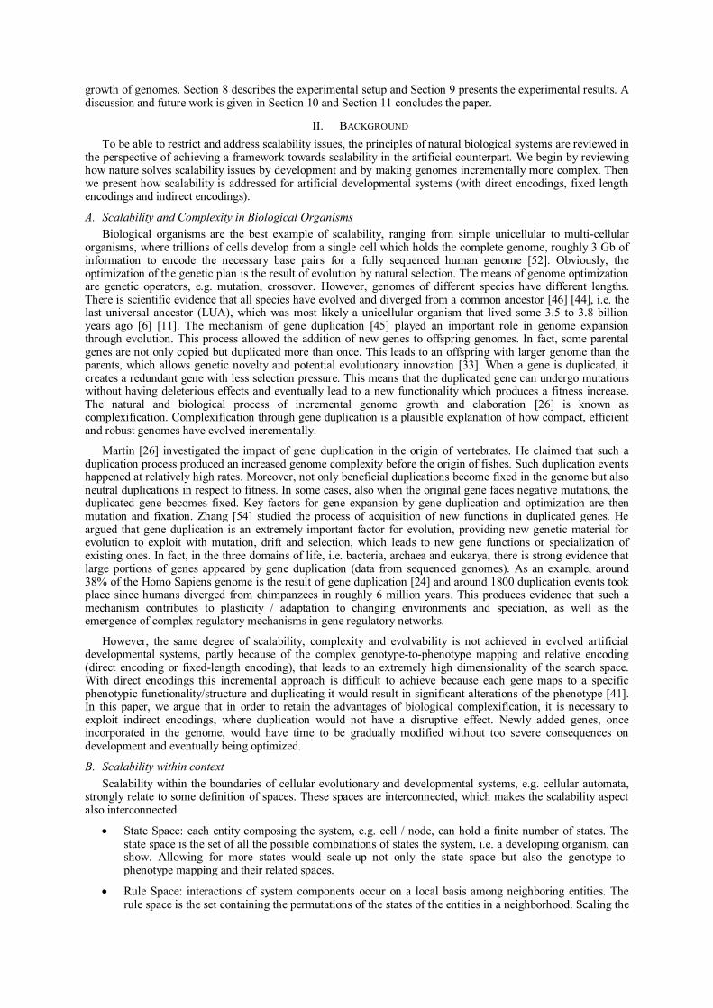
growth of genomes. Section 8 describes the experimental setup and Section 9 presents the experimental results. A discussion and future work is given in Section 10 and Section 11 concludes the paper.
II. BACKGROUND
To be able to restrict and address scalability issues, the principles of natural biological systems are reviewed in the perspective of achieving a framework towards scalability in the artificial counterpart. We begin by reviewing how nature solves scalability issues by development and by making genomes incrementally more complex. Then we present how scalability is addressed for artificial developmental systems (with direct encodings, fixed length encodings and indirect encodings).
A. Scalability and Complexity in Biological Organisms
Biological organisms are the best example of scalability, ranging from simple unicellular to multi-cellular organisms, where trillions of cells develop from a single cell which holds the complete genome, roughly 3 Gb of information to encode the necessary base pairs for a fully sequenced human genome [52]. Obviously, the optimization of the genetic plan is the result of evolution by natural selection. The means of genome optimization are genetic operators, e.g. mutation, crossover. However, genomes of different species have different lengths. There is scientific evidence that all species have evolved and diverged from a common ancestor [46] [44], i.e. the last universal ancestor (LUA), which was most likely a unicellular organism that lived some 3.5 to 3.8 billion years ago [6] [11]. The mechanism of gene duplication [45] played an important role in genome expansion through evolution. This process allowed the addition of new genes to offspring genomes. In fact, some parental genes are not only copied but duplicated more than once. This leads to an offspring with larger genome than the parents, which allows genetic novelty and potential evolutionary innovation [33]. When a gene is duplicated, it creates a redundant gene with less selection pressure. This means that the duplicated gene can undergo mutations without having deleterious effects and eventually lead to a new functionality which produces a fitness increase. The natural and biological process of incremental genome growth and elaboration [26] is known as complexification. Complexification through gene duplication is a plausible explanation of how compact, efficient and robust genomes have evolved incrementally.
Martin [26] investigated the impact of gene duplication in the origin of vertebrates. He claimed that such a duplication process produced an increased genome complexity before the origin of fishes. Such duplication events happened at relatively high rates. Moreover, not only beneficial duplications become fixed in the genome but also neutral duplications in respect to fitness. In some cases, also when the original gene faces negative mutations, the duplicated gene becomes fixed. Key factors for gene expansion by gene duplication and optimization are then mutation and fixation. Zhang [54] studied the process of acquisition of new functions in duplicated genes. He argued that gene duplication is an extremely important factor for evolution, providing new genetic material for evolution to exploit with mutation, drift and selection, which leads to new gene functions or specialization of existing ones. In fact, in the three domains of life, i.e. bacteria, archaea and eukarya, there is strong evidence that large portions of genes appeared by gene duplication (data from sequenced genomes). As an example, around 38% of the Homo Sapiens genome is the result of gene duplication [24] and around 1800 duplication events took place since humans diverged from chimpanzees in roughly 6 million years. This produces evidence that such a mechanism contributes to plasticity / adaptation to changing environments and speciation, as well as the emergence of complex regulatory mechanisms in gene regulatory networks.
However, the same degree of scalability, complexity and evolvability is not achieved in evolved artificial developmental systems, partly because of the complex genotype-to-phenotype mapping and relative encoding (direct encoding or fixed-length encoding), that leads to an extremely high dimensionality of the search space. With direct encodings this incremental approach is difficult to achieve because each gene maps to a specific phenotypic functionality/structure and duplicating it would result in significant alterations of the phenotype [41]. In this paper, we argue that in order to retain the advantages of biological complexification, it is necessary to exploit indirect encodings, where duplication would not have a disruptive effect. Newly added genes, once incorporated in the genome, would have time to be gradually modified without too severe consequences on development and eventually being optimized.
B. Scalability within context
Scalability within the boundaries of cellular evolutionary and developmental systems, e.g. cellular automata, strongly relate to some definition of spaces. These spaces are interconnected, which makes the scalability aspect also interconnected.
State Space: each entity composing the system, e.g. cell / node, can hold a finite number of states. The state space is the set of all the possible combinations of states the system, i.e. a developing organism, can show. Allowing for more states would scale-up not only the state space but also the genotype-to-phenotype mapping and their related spaces.
Rule Space: interactions of system components occur on a local basis among neighboring entities. The rule space is the set containing the permutations of the states of the entities in a neighborhood. Scaling the
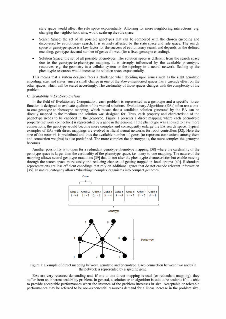
state space would affect the rule space exponentially. Allowing for more neighboring interactions, e.g. changing the neighborhood size, would scale-up the rule space.
Search Space: the set of all possible genotypes that can be composed with the chosen encoding and discovered by evolutionary search. It is strongly affected by the state space and rule space. The search space or genotype space is a key factor for the success of evolutionary search and depends on the defined encoding, genotype size and number of genes allowed (for a fixed genotype encoding).
Solution Space: the set of all possible phenotypes. The solution space is different from the search space due to the genotype-to-phenotype mapping. It is strongly influenced by the available phenotypic resources, e.g. the geometry in a cellular system or the topology in a neural network. Scaling-up the phenotypic resources would increase the solution space exponentially.
This means that a system designer faces a challenge when deciding upon issues such as the right genotype encoding, size, and states, since a small change in one of the above-mentioned spaces has a cascade effect on the other spaces, which will be scaled accordingly. The cardinality of those spaces changes with the complexity of the problem.
C. Scalability in EvoDevo Systems
In the field of Evolutionary Computation, each problem is represented as a genotype and a specific fitness function is designed to evaluate qualities of the wanted solutions. Evolutionary Algorithms (EAs) often use a one-to-one genotype-to-phenotype mapping, which means that a candidate solution generated by the EA can be directly mapped to the medium the solution was designed for. Thus, each property and characteristic of the phenotype needs to be encoded in the genotype. Figure 1 presents a direct mapping where each phenotypic property (network connection) is represented by a gene in the genome. If the phenotype was allowed to have more connections, the genotype would become more complex and consequently enlarge the EA search space. Typical examples of EAs with direct mappings are evolved artificial neural networks for robot controllers [32]. Here the size of the network is predefined and thus the available number of genes (to represent connections among them and connection weights) is also predefined. The more complex the phenotype is, the more complex the genotype becomes.
Another possibility is to open for a redundant genotype-phenotype mapping [38] where the cardinality of the genotype space is larger than the cardinality of the phenotype space, i.e. many-to-one mapping. The nature of the mapping allows neutral genotype mutations [39] that do not alter the phenotypic characteristics but enable moving through the search space more easily and reducing chances of getting trapped in local optima [40]. Redundant representations are less efficient encodings that rely on additional genes that do not encode relevant information [35]. In nature, ontogeny allows “shrinking” complex organisms into compact genomes.
Figure 1: Example of direct mapping between genotype and phenotype. Each connection between two nodes in the network is represented by a specific gene.
EAs are very resource demanding and, if one-to-one direct mapping is used (or redundant mapping), they suffer from an inherent scalability problem. In general, a solution or an algorithm is said to be scalable if it is able to provide acceptable performances when the instance of the problem increases in size. Acceptable or tolerable performances may be referred to be non-exponential resources demand for a linear increase in the problem size.
This is not the case for EAs, where an increase of the problem size does not reflect a proportional increase in the search space. One solution for the resource-demanding trait of EAs is to take inspiration from nature and somehow shrink the genotype, i.e. indirect mapping. This reduces the overall complexity of the genotype (and the search space magnitude) while adding more complexity to the genotype-to-phenotype mapping and the underlying development process. Thus the challenges are finding an efficient developmental mechanism and a suitable indirect representation that is able to exploit such development process.
Even though developmental systems are widely used [49, 7, 27, 14, 42], the genotype representation scalability challenge still exists. For several developmental systems it would not be feasible to fully specify all the possible regulatory combinations in the genotype, e.g. complete regulatory information for Tufte’s CA-based model [48] would require the specification of 545 regulatory possibilities, Miller and Banzhaf’s cellular developmental Cartesian Genetic Programming (CGP) model [27] a total of 7689, von Neumann’s universal constructor [28] 295 combinations. For many systems, using fixed-length genotypes containing only a subset of all the possible regulatory combinations is a necessity. In cellular models the total possible number of regulatory combinations is NK, where N is the number of possible states each cell can hold and K is the neighborhood. Bidlo [4] for his instruction-based cellular model with four possible cell states and neighborhood of size 5 used a restricted transition function of only 10 entries, Tufte [47] had a model with 13 possible cell states and five neighbors whether the available regulatory rule-set was restricted to 64. Tufte and Thomassen [51] investigated scaling of genomes with fixed-length representation and allowed 4, 5, 6 and 32 regulation rules out of the possible regulatory information based on three cell types and five neighbors (13 cell types for genome of size 32). In all such cases, the maximum representation was pre-defined and could not change during evolution. The available regulatory information was designed a priori by trial and error or by estimation and did not guarantee that a possible solution could be found at all or that the same solutions could be achieved with a smaller genotype representation. Nonetheless, the maximum complexity of the system was predetermined, in the sense that the reachable search space was shrunk by the chosen representation. If one wanted to scale up the system by allowing a larger neighborhood or more available cell states, the chosen genotypes may not have been large enough to represent a candidate solution, as the cardinality of the mapping would be changed.
An alternative that can scale both genotype and phenotype information is to open for a variable length genome. An example of variable-length general encoding that can be applied for indirect construction of phenotypes [36] is Genetic Programming [21]. If a mechanism of adding genes through gene duplication is allowed, it is possible to incrementally grow the genome size. This complexification strategy may help to solve the genotype representation scalability problem. Previous work was done towards achieving genome size expansion, for example [5], [13], [20], [25]. Federici and Downing [9] investigated neutral gene duplication in a cellular model with environmental chemicals. They studied genome scalability with direct encoding and embryonal stages, using a gene regulatory model based on recursive neural networks (RNN). Stanley and Miikkulainen [43] introduced NeuroEvolution of Augmenting topologies (NEAT), a complexification method for the incremental evolution of neural network architectures. Their main goal was to evolve robot controllers with direct encodings through gene duplication. They argued that incremental evolution of complex neural network genomes relies on three main technical components: meaningful crossover by means of historical markings for gene alignment, innovation through speciation which enables optimization, start from minimal genomes and allow incremental size increase. Taking inspiration from the presented research on complexification of developmental systems with direct encodings, we investigate the basic idea using indirect encodings [41]. An incremental evolution of genome representations may have the potential for exploration on developmental systems with an indirect genotype-to-phenotype mapping.
III. FRAMEWORK FOR INCREMENTAL EVOLUTION OF GENOME REPRESENTATIONS
This section presents a possible framework for incremental evolution of genome representations on artificial cellular organisms with indirect encodings. Using indirect encodings is a necessity, since for highly complex systems (potentially at biological complexity levels), the search in the space of final solutions would be intractable [41].
Conventional genetic algorithms consist of few steps, which can be summarized as follows:
1. Initialize random population;
2. Compute fitness;
3. Proportionate selection;
4. Crossover and mutation;
5. Generate new population;
6. Jump to step 2 and repeat until the convergence criteria is satisfied.
For embryomorphic systems, the fitness evaluation cannot be performed directly on the individuals in the population, due to the indirect mapping between genotype and phenotype. As such, each genotype is developed starting from a single cell, i.e. zygote, to a multi-cellular organism (phenotype) which is subject to fitness
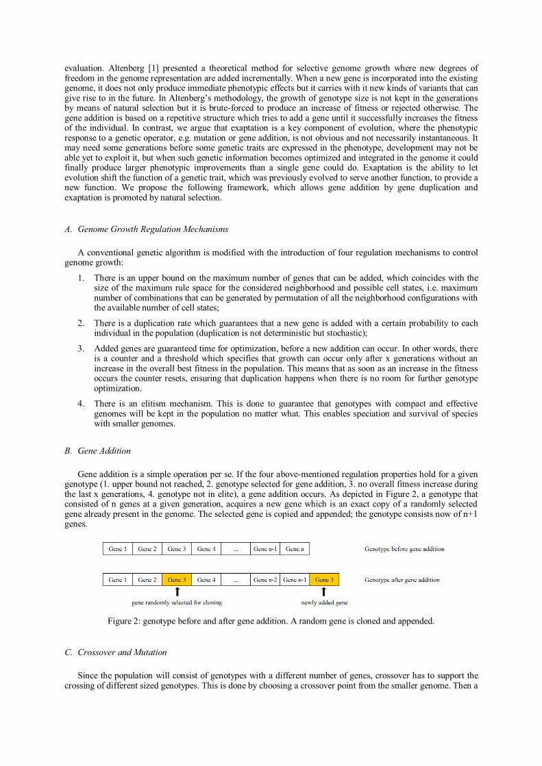
evaluation. Altenberg [1] presented a theoretical method for selective genome growth where new degrees of freedom in the genome representation are added incrementally. When a new gene is incorporated into the existing genome, it does not only produce immediate phenotypic effects but it carries with it new kinds of variants that can give rise to in the future. In Altenberg’s methodology, the growth of genotype size is not kept in the generations by means of natural selection but it is brute-forced to produce an increase of fitness or rejected otherwise. The gene addition is based on a repetitive structure which tries to add a gene until it successfully increases the fitness of the individual. In contrast, we argue that exaptation is a key component of evolution, where the phenotypic response to a genetic operator, e.g. mutation or gene addition, is not obvious and not necessarily instantaneous. It may need some generations before some genetic traits are expressed in the phenotype, development may not be able yet to exploit it, but when such genetic information becomes optimized and integrated in the genome it could finally produce larger phenotypic improvements than a single gene could do. Exaptation is the ability to let evolution shift the function of a genetic trait, which was previously evolved to serve another function, to provide a new function. We propose the following framework, which allows gene addition by gene duplication and exaptation is promoted by natural selection.
A. Genome Growth Regulation Mechanisms
A conventional genetic algorithm is modified with the introduction of four regulation mechanisms to control
genome growth:
1. There is an upper bound on the maximum number of genes that can be added, which coincides with the size of the maximum rule space for the considered neighborhood and possible cell states, i.e. maximum number of combinations that can be generated by permutation of all the neighborhood configurations with the available number of cell states;
2. There is a duplication rate which guarantees that a new gene is added with a certain probability to each individual in the population (duplication is not deterministic but stochastic);
3. Added genes are guaranteed time for optimization, before a new addition can occur. In other words, there is a counter and a threshold which specifies that growth can occur only after x generations without an increase in the overall best fitness in the population. This means that as soon as an increase in the fitness occurs the counter resets, ensuring that duplication happens when there is no room for further genotype optimization.
4. There is an elitism mechanism. This is done to guarantee that genotypes with compact and effective genomes will be kept in the population no matter what. This enables speciation and survival of species with smaller genomes.
B. Gene Addition
Gene addition is a simple operation per se. If the four above-mentioned regulation properties hold for a given genotype (1. upper bound not reached, 2. genotype selected for gene addition, 3. no overall fitness increase during the last x generations, 4. genotype not in elite), a gene addition occurs. As depicted in Figure 2, a genotype that consisted of n genes at a given generation, acquires a new gene which is an exact copy of a randomly selected gene already present in the genome. The selected gene is copied and appended; the genotype consists now of n+1 genes.
Figure 2: genotype before and after gene addition. A random gene is cloned and appended.
C. Crossover and Mutation
Since the population will consist of genotypes with a different number of genes, crossover has to support the crossing of different sized genotypes. This is done by choosing a crossover point from the smaller genome. Then a
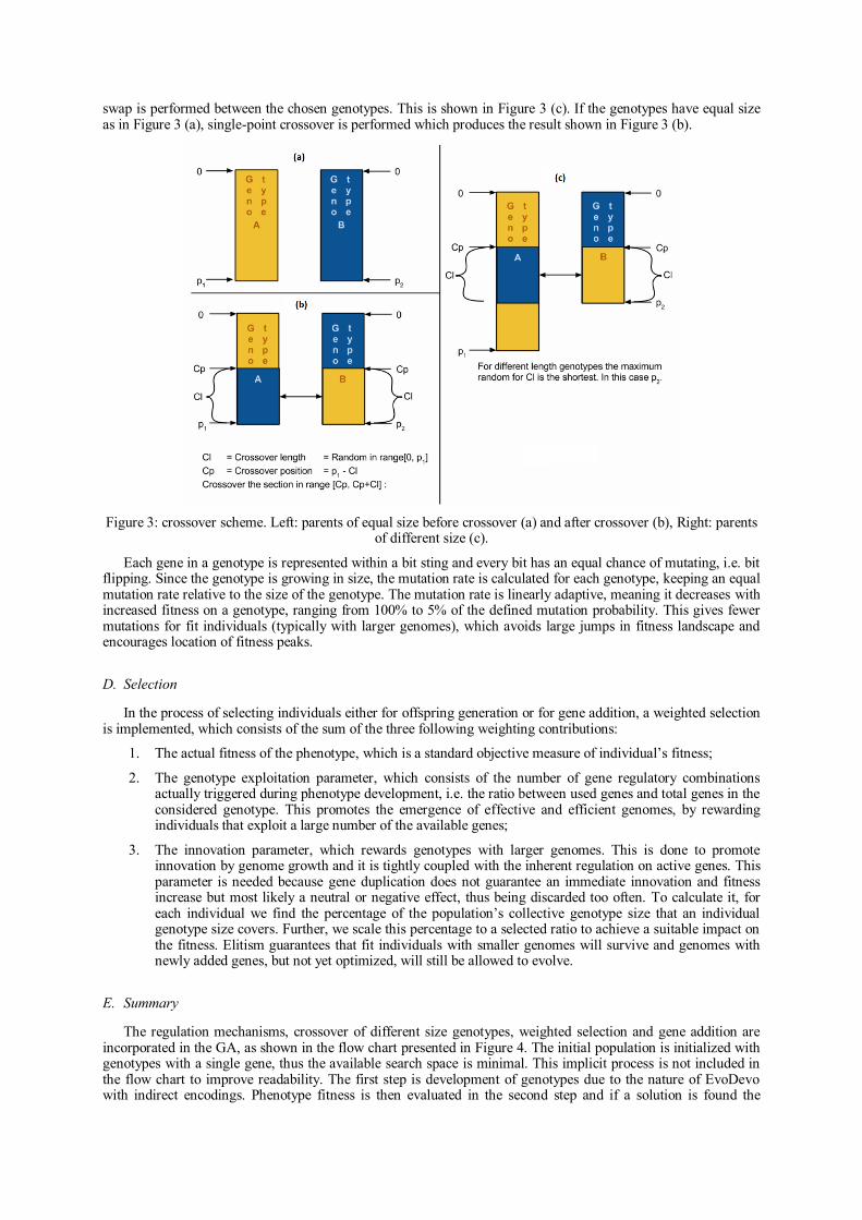
swap is performed between the chosen genotypes. This is shown in Figure 3 (c). If the genotypes have equal size as in Figure 3 (a), single-point crossover is performed which produces the result shown in Figure 3 (b).
Figure 3: crossover scheme. Left: parents of equal size before crossover (a) and after crossover (b), Right: parents of different size (c).
Each gene in a genotype is represented within a bit sting and every bit has an equal chance of mutating, i.e. bit flipping. Since the genotype is growing in size, the mutation rate is calculated for each genotype, keeping an equal mutation rate relative to the size of the genotype. The mutation rate is linearly adaptive, meaning it decreases with increased fitness on a genotype, ranging from 100% to 5% of the defined mutation probability. This gives fewer mutations for fit individuals (typically with larger genomes), which avoids large jumps in fitness landscape and encourages location of fitness peaks.
D. Selection
In the process of selecting individuals either for offspring generation or for gene addition, a weighted selection is implemented, which consists of the sum of the three following weighting contributions:
1. The actual fitness of the phenotype, which is a standard objective measure of individual’s fitness;
2. The genotype exploitation parameter, which consists of the number of gene regulatory combinations actually triggered during phenotype development, i.e. the ratio between used genes and total genes in the considered genotype. This promotes the emergence of effective and efficient genomes, by rewarding individuals that exploit a large number of the available genes;
3. The innovation parameter, which rewards genotypes with larger genomes. This is done to promote innovation by genome growth and it is tightly coupled with the inherent regulation on active genes. This parameter is needed because gene duplication does not guarantee an immediate innovation and fitness increase but most likely a neutral or negative effect, thus being discarded too often. To calculate it, for each individual we find the percentage of the population’s collective genotype size that an individual genotype size covers. Further, we scale this percentage to a selected ratio to achieve a suitable impact on the fitness. Elitism guarantees that fit individuals with smaller genomes will survive and genomes with newly added genes, but not yet optimized, will still be allowed to evolve.
E. Summary
The regulation mechanisms, crossover of different size genotypes, weighted selection and gene addition are incorporated in the GA, as shown in the flow chart presented in Figure 4. The initial population is initialized with genotypes with a single gene, thus the available search space is minimal. This implicit process is not included in the flow chart to improve readability. The first step is development of genotypes due to the nature of EvoDevo with indirect encodings. Phenotype fitness is then evaluated in the second step and if a solution is found the
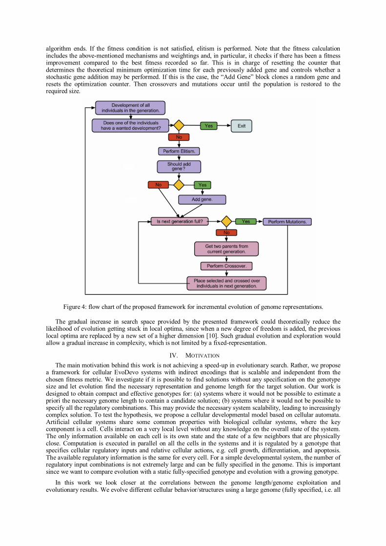
algorithm ends. If the fitness condition is not satisfied, elitism is performed. Note that the fitness calculation includes the above-mentioned mechanisms and weightings and, in particular, it checks if there has been a fitness improvement compared to the best fitness recorded so far. This is in charge of resetting the counter that determines the theoretical minimum optimization time for each previously added gene and controls whether a stochastic gene addition may be performed. If this is the case, the “Add Gene” block clones a random gene and resets the optimization counter. Then crossovers and mutations occur until the population is restored to the required size.
Figure 4: flow chart of the proposed framework for incremental evolution of genome representations.
The gradual increase in search space provided by the presented framework could theoretically reduce the likelihood of evolution getting stuck in local optima, since when a new degree of freedom is added, the previous local optima are replaced by a new set of a higher dimension [10]. Such gradual evolution and exploration would allow a gradual increase in complexity, which is not limited by a fixed-representation.
IV. MOTIVATION
The main motivation behind this work is not achieving a speed-up in evolutionary search. Rather, we propose a framework for cellular EvoDevo systems with indirect encodings that is scalable and independent from the chosen fitness metric. We investigate if it is possible to find solutions without any specification on the genotype size and let evolution find the necessary representation and genome length for the target solution. Our work is designed to obtain compact and effective genotypes for: (a) systems where it would not be possible to estimate a priori the necessary genome length to contain a candidate solution; (b) systems where it would not be possible to specify all the regulatory combinations. This may provide the necessary system scalability, leading to increasingly complex solution. To test the hypothesis, we propose a cellular developmental model based on cellular automata. Artificial cellular systems share some common properties with biological cellular systems, where the key component is a cell. Cells interact on a very local level without any knowledge on the overall state of the system. The only information available on each cell is its own state and the state of a few neighbors that are physically close. Computation is executed in parallel on all the cells in the systems and it is regulated by a genotype that specifies cellular regulatory inputs and relative cellular actions, e.g. cell growth, differentiation, and apoptosis. The available regulatory information is the same for every cell. For a simple developmental system, the number of regulatory input combinations is not extremely large and can be fully specified in the genome. This is important since we want to compare evolution with a static fully-specified genotype and evolution with a growing genotype.
In this work we look closer at the correlations between the genome length/genome exploitation and evolutionary results. We evolve different cellular behavior/structures using a large genome (fully specified, i.e. all
the possible regulatory input combinations), a growing genotype and a small genome (a restricted genome pool out of all the possible regulatory input combinations). By comparing these methods to each other, we can get an understanding of how restrains affect the evolved organism. We consider the genome usage for the evolved solutions on different complexities. Further, we pose some answers to questions such as: Are we going to find that growing a genotype produces compact and effective genotypes? Or will the results be similar to those of an organism evolved with a large genotype? How will this type of evolution scale? Could a cellular EvoDevo-system which evolves organisms with a growing genotype exhibit emergent or implicit behavior not found in organisms evolved with a static large genotype? Will this kind of evolution actually be able to produce results at all?
Once the proposed framework is found to be able to evolve a solution with a minimalistic developmental system, we scale-up the system complexity and available resources. A simple way of making Cellular Systems capable of very complex behavior is to increase the amount of cell states, which in turn increases the regulatory rule space, the evolutionary search space, and the system state space exponentially. If the proposed framework is able to achieve results while changing the number of cell states, it would mean that the framework could support growing evolution in both search and state space, which means it would ideally allow to tackle problems of increasing complexity. The presented experiments are mainly to investigate if the growth evolution function is able to create solutions with more cell states. We also investigate if the growing evolution function is able to find solutions in cellular spaces with different size geometries. By increasing the geometry, the solution space expands considerably, i.e. the number of states the system can exhibit.
V. SCALABILITY
In today’s society, we often use computers to solve very large problems. For instance, extensive problems with a vast amount of variable parameters can be tackled with an EA, but even so it requires much computational power / time and often produces large solutions (solution here refers to the specification of a candidate solution in the genotype). Having a good understanding of scalability can help both the usage of computational power, the size of the solutions, and might even be able to shrink the size of the problem. To increase EA scalability to large problems, development has been widely used, which creates small solutions to problems that normally require larger solutions. This again makes the solutions manageable, making scaling a valuable tool. EvoDevo systems are often applied within the field of cellular development, e.g. CA, which makes cellular systems already a method that scales well [37]. One way in which scalability can be increased is by reducing the state or search space for a wanted solution, which essentially reduces the size of the fitness landscape, making systems scale to solve larger problems. Knowing what makes algorithms create solutions that are scalable in geometry (or resources) can reduce the problem, making the resource consumption manageable. Having a good understanding of scalability gives a better utilization of resources, and makes it possible to create solutions to problems which one normally does not have enough resources to solve, or makes runtimes of currently solvable problems faster. There are of course many other ways to reduce the real runtime of an EA, for instance massively distributed or parallelized algorithms. But these will also benefit from a smaller search space and state space, which can be achieved by scaling in efficiency. By understanding how solutions scale in geometry, it can become possible to evolve small solutions that scale-up to larger geometries with linear increase, or without the loss of functionality.
At the design stage of a cellular EvoDevo system, the choices of the genotype size/encoding, the number of system states and the available resources have an impact on the search space, state space and solution space [2]. In the next sections, all these three relevant scalability aspects are addressed.
A. Scalability in effectiveness (search space)
Effectiveness with regards to an EA is the measure of the amount of genes used in an evolved solution compared to the minimum amount of genes needed for the solution to work. Also, the amount of genes used in an evolved solution compared to the amount of genes available for each individual in a population during evolutionary search. With regards to a cellular system, effectiveness is the measure of used regulatory input combinations, i.e. neighborhood configurations, compared to theoretical maximum regulatory information. This is a key factor for scalability since reducing the genotype size greatly decreases the search space.
In the first set of experiments we fix the target phenotypic complexity/behavior and the CA geometry and evolve solutions with a full genotype, i.e. all the possible regulatory information are fully specified (maximum genome length for the chosen cellular model). The results are compared to solutions obtained with a restricted gene pool where only a limited amount of regulatory combinations can be specified. Finally we evolve solutions with our proposed framework on incremental growth of genome representations, which automatically increases the size of the genotypes. We evaluate the genotypes of the found solutions in terms of compactness, i.e. the size of the whole genotype, and effectiveness, i.e. number of triggered genes during development in contrast to the total available genes in the genotype solutions.
B. Scalability of states (state space)
In the second set of experiments we investigate if the proposed framework is able to evolve solutions when the state space increases. For a cellular system, this means scaling-up the number of available states each cell can
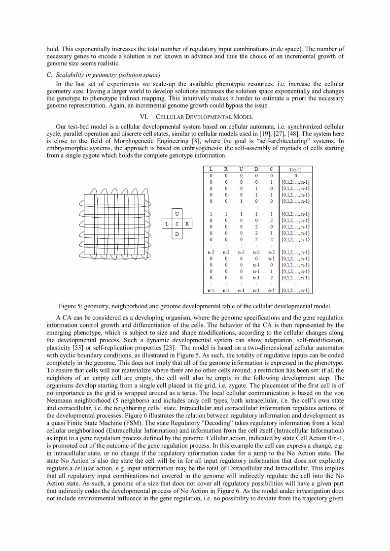
hold. This exponentially increases the total number of regulatory input combinations (rule space). The number of necessary genes to encode a solution is not known in advance and thus the choice of an incremental growth of genome size seems realistic.
C. Scalability in geometry (solution space)
In the last set of experiments we scale-up the available phenotypic resources, i.e. increase the cellular geometry size. Having a larger world to develop solutions increases the solution space exponentially and changes the genotype to phenotype indirect mapping. This intuitively makes it harder to estimate a priori the necessary genome representation. Again, an incremental genome growth could bypass the issue.
VI. CELLULAR DEVELOPMENTAL MODEL
Our test-bed model is a cellular developmental system based on cellular automata, i.e. synchronized cellular cycle, parallel operation and discrete cell states, similar to cellular models used in [19], [27], [48]. The system here is close to the field of Morphogenetic Engineering [8], where the goal is “self-architecturing” systems. In embryomorphic systems, the approach is based on embryogenesis: the self-assembly of myriads of cells starting from a single zygote which holds the complete genotype information.
Figure 5: geometry, neighborhood and genome developmental table of the cellular developmental model.
A CA can be considered as a developing organism, where the genome specifications and the gene regulation information control growth and differentiation of the cells. The behavior of the CA is then represented by the
emerging phenotype, which is subject to size and shape modifications, according to the cellular changes along
the developmental process. Such a dynamic developmental system can show adaptation, self-modification,
plasticity [53] or self-replication properties [23]. The model is based on a two-dimensional cellular automaton
with cyclic boundary conditions, as illustrated in Figure 5. As such, the totality of regulative inputs can be coded
completely in the genome. This does not imply that all of the genome information is expressed in the phenotype.
To ensure that cells will not materialize where there are no other cells around, a restriction has been set: if all the
neighbors of an empty cell are empty, the cell will also be empty in the following development step. The
organisms develop starting from a single cell placed in the grid, i.e. zygote. The placement of the first cell is of
no importance as the grid is wrapped around as a torus. The local cellular communication is based on the von
Neumann neighborhood (5 neighbors) and includes only cell types, both intracellular, i.e. the cell’s own state
and extracellular, i.e. the neighboring cells’ state. Intracellular and extracellular information regulates actions of the developmental processes. Figure 6 illustrates the relation between regulatory information and development as
a quasi Finite State Machine (FSM). The state Regulatory ”Decoding” takes regulatory information from a local
cellular neighborhood (Extracellular Information) and information from the cell itself (Intracellular Information)
as input to a gene regulation process defined by the genome. Cellular action, indicated by state Cell Action 0/n-1,
is promoted out of the outcome of the gene regulation process. In this example the cell can express a change, e.g.
in intracellular state, or no change if the regulatory information codes for a jump to the No Action state. The
state No Action is also the state the cell will be in for all input regulatory information that does not explicitly
regulate a cellular action, e.g. input information may be the total of Extracellular and Intracellular. This implies
that all regulatory input combinations not covered in the genome will indirectly regulate the cell into the No
Action state. As such, a genome of a size that does not cover all regulatory possibilities will have a given part
that indirectly codes the developmental process of No Action in Figure 6. As the model under investigation does not include environmental influence in the gene regulation, i.e. no possibility to deviate from the trajectory given
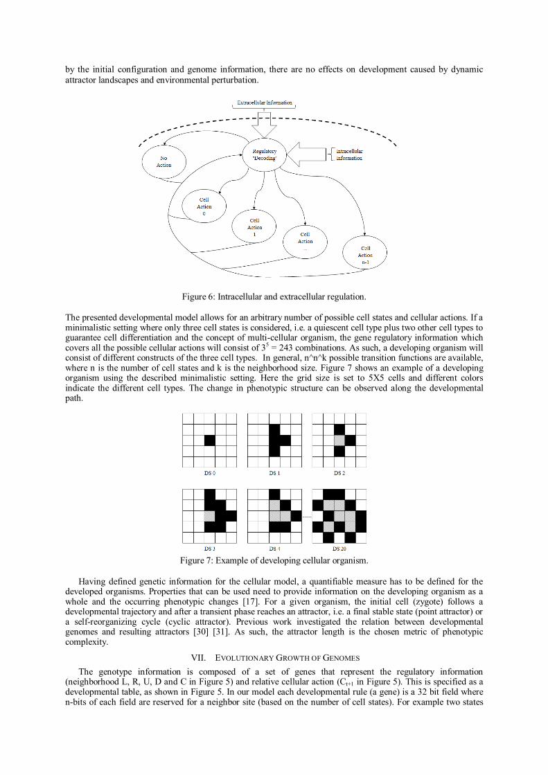
by the initial configuration and genome information, there are no effects on development caused by dynamic
attractor landscapes and environmental perturbation.
Figure 6: Intracellular and extracellular regulation.
The presented developmental model allows for an arbitrary number of possible cell states and cellular actions. If a minimalistic setting where only three cell states is considered, i.e. a quiescent cell type plus two other cell types to guarantee cell differentiation and the concept of multi-cellular organism, the gene regulatory information which covers all the possible cellular actions will consist of 35 = 243 combinations. As such, a developing organism will consist of different constructs of the three cell types. In general, n^n^k possible transition functions are available, where n is the number of cell states and k is the neighborhood size. Figure 7 shows an example of a developing organism using the described minimalistic setting. Here the grid size is set to 5X5 cells and different colors indicate the different cell types. The change in phenotypic structure can be observed along the developmental path.
Figure 7: Example of developing cellular organism.
Having defined genetic information for the cellular model, a quantifiable measure has to be defined for the developed organisms. Properties that can be used need to provide information on the developing organism as a whole and the occurring phenotypic changes [17]. For a given organism, the initial cell (zygote) follows a developmental trajectory and after a transient phase reaches an attractor, i.e. a final stable state (point attractor) or a self-reorganizing cycle (cyclic attractor). Previous work investigated the relation between developmental genomes and resulting attractors [30] [31]. As such, the attractor length is the chosen metric of phenotypic complexity.
VII. EVOLUTIONARY GROWTH OF GENOMES
The genotype information is composed of a set of genes that represent the regulatory information (neighborhood L, R, U, D and C in Figure 5) and relative cellular action (Ct+1 in Figure 5). This is specified as a developmental table, as shown in Figure 5. In our model each developmental rule (a gene) is a 32 bit field where n-bits of each field are reserved for a neighbor site (based on the number of cell states). For example two states
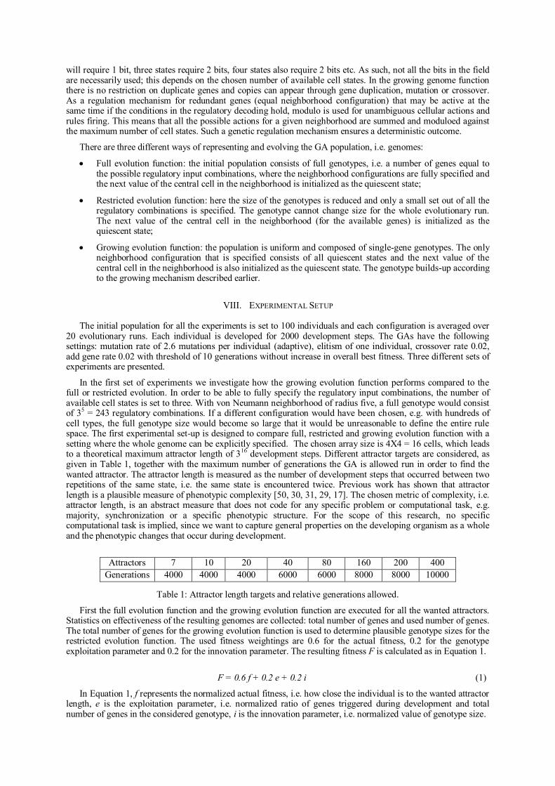
will require 1 bit, three states require 2 bits, four states also require 2 bits etc. As such, not all the bits in the field are necessarily used; this depends on the chosen number of available cell states. In the growing genome function there is no restriction on duplicate genes and copies can appear through gene duplication, mutation or crossover. As a regulation mechanism for redundant genes (equal neighborhood configuration) that may be active at the same time if the conditions in the regulatory decoding hold, modulo is used for unambiguous cellular actions and rules firing. This means that all the possible actions for a given neighborhood are summed and moduloed against the maximum number of cell states. Such a genetic regulation mechanism ensures a deterministic outcome.
There are three different ways of representing and evolving the GA population, i.e. genomes:
Full evolution function: the initial population consists of full genotypes, i.e. a number of genes equal to the possible regulatory input combinations, where the neighborhood configurations are fully specified and the next value of the central cell in the neighborhood is initialized as the quiescent state;
Restricted evolution function: here the size of the genotypes is reduced and only a small set out of all the regulatory combinations is specified. The genotype cannot change size for the whole evolutionary run. The next value of the central cell in the neighborhood (for the available genes) is initialized as the quiescent state;
Growing evolution function: the population is uniform and composed of single-gene genotypes. The only neighborhood configuration that is specified consists of all quiescent states and the next value of the central cell in the neighborhood is also initialized as the quiescent state. The genotype builds-up according to the growing mechanism described earlier.
VIII. EXPERIMENTAL SETUP
The initial population for all the experiments is set to 100 individuals and each configuration is averaged over 20 evolutionary runs. Each individual is developed for 2000 development steps. The GAs have the following settings: mutation rate of 2.6 mutations per individual (adaptive), elitism of one individual, crossover rate 0.02, add gene rate 0.02 with threshold of 10 generations without increase in overall best fitness. Three different sets of experiments are presented.
In the first set of experiments we investigate how the growing evolution function performs compared to the full or restricted evolution. In order to be able to fully specify the regulatory input combinations, the number of available cell states is set to three. With von Neumann neighborhood of radius five, a full genotype would consist of 35 = 243 regulatory combinations. If a different configuration would have been chosen, e.g. with hundreds of cell types, the full genotype size would become so large that it would be unreasonable to define the entire rule space. The first experimental set-up is designed to compare full, restricted and growing evolution function with a setting where the whole genome can be explicitly specified. The chosen array size is 4X4 = 16 cells, which leads to a theoretical maximum attractor length of 316 development steps. Different attractor targets are considered, as given in Table 1, together with the maximum number of generations the GA is allowed run in order to find the wanted attractor. The attractor length is measured as the number of development steps that occurred between two repetitions of the same state, i.e. the same state is encountered twice. Previous work has shown that attractor length is a plausible measure of phenotypic complexity [50, 30, 31, 29, 17]. The chosen metric of complexity, i.e. attractor length, is an abstract measure that does not code for any specific problem or computational task, e.g. majority, synchronization or a specific phenotypic structure. For the scope of this research, no specific computational task is implied, since we want to capture general properties on the developing organism as a whole and the phenotypic changes that occur during development.
Attractors 7 10 20 40 80 160 200 400
Generations 4000 4000 4000 6000 6000 8000 8000 10000
Table 1: Attractor length targets and relative generations allowed.
First the full evolution function and the growing evolution function are executed for all the wanted attractors. Statistics on effectiveness of the resulting genomes are collected: total number of genes and used number of genes. The total number of genes for the growing evolution function is used to determine plausible genotype sizes for the restricted evolution function. The used fitness weightings are 0.6 for the actual fitness, 0.2 for the genotype exploitation parameter and 0.2 for the innovation parameter. The resulting fitness F is calculated as in Equation 1.
F = 0.6 f + 0.2 e + 0.2 i (1)
In Equation 1, f represents the normalized actual fitness, i.e. how close the individual is to the wanted attractor length, e is the exploitation parameter, i.e. normalized ratio of genes triggered during development and total number of genes in the considered genotype, i is the innovation parameter, i.e. normalized value of genotype size.
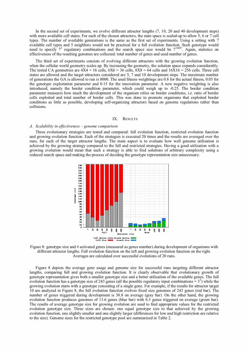
In the second set of experiments, we evolve different attractor lengths (7, 10, 20 and 40 development steps) with more available cell states. For each of the chosen attractors, the state space is scaled-up to allow 5, 6 or 7 cell types. The number of available generations is the same as the first set of experiments. Using a setting with 7 available cell types and 5 neighbors would not be practical for a full evolution function. Such genotype would need to specify 75 regulatory combinations and the search space size would be 716807. Again, statistics on effectiveness of the resulting genomes are collected: total number of genes and used number of genes.
The third set of experiments consists of evolving different attractors with the growing evolution function, when the cellular world geometry scales up. By increasing the geometry, the solution space expands considerably. The tested CA geometries are 4X4 = 16 cells, 6X6 = 36 cells, 8X8 = 64 cells and 16X16 = 256 cells. Three cell states are allowed and the target attractors considered are 5, 7 and 10 development steps. The maximum number of generations the GA is allowed to run is 8000. The used fitness weightings are 0.8 for the actual fitness, 0.05 for the genotype exploitation parameter and 0.15 for the innovation parameter. A new negative weighting is also introduced, namely the border condition parameter, which could weigh up to -0.25. The border condition parameter measures how much the development of the organism relies on border conditions, i.e. ratio of border cells exploited and total number of border cells. This was done to promote organisms that exploited border conditions as little as possible, developing self-organizing attractors based on genome regulations rather than collisions.
IX. RESULTS
A. Scalability in effectiveness – genome comparison
Three evolutionary strategies are tested and compared: full evolution function, restricted evolution function and growing evolution function. Each of the strategies is executed 20 times and the results are averaged over the runs, for each of the target attractor lengths. The main aspect is to evaluate how well genome utilization is achieved by the growing strategy compared to the full and restricted strategies. Having a good utilization with a growing evolution would mean that such a strategy is able to find solutions of arbitrary complexity using a reduced search space and making the process of deciding the genotype representation size unnecessary.
Figure 8: genotype size and # activated genes (measured as genes number) during development of organisms with different attractor lengths. Full evolution function on the left and growing evolution function on the right.
Averages are calculated over successful evolutions of 20 runs.
Figure 8 depicts the average gene usage and genome size for successful runs targeting different attractor lengths, comparing full and growing evolution function. It is clearly observable that evolutionary growth of genotype representation gives both a smaller genotype size and a better utilization of the available genes. The full evolution function has a genotype size of 243 genes (all the possible regulatory input combinations = 35) while the growing evolution starts with a genotype consisting of a single gene. For example, if the results for attractor target 10 are analyzed in Figure 8, the full evolution function evolves fixed size genomes of 243 genes (red bar). The number of genes triggered during development is 38.8 on average (gray bar). On the other hand, the growing evolution function produces genomes of 13.6 genes (blue bar) with 6.3 genes triggered on average (green bar). The results of average genotype size for growing evolution are used to find appropriate values for the restricted evolution genotype size. Three sizes are chosen: one equal genotype size to that achieved by the growing evolution function, one slightly smaller and one slightly larger (differences for low and high restriction are relative to the size). Genome sizes for the restricted genotype pool are summarized in Table 2.
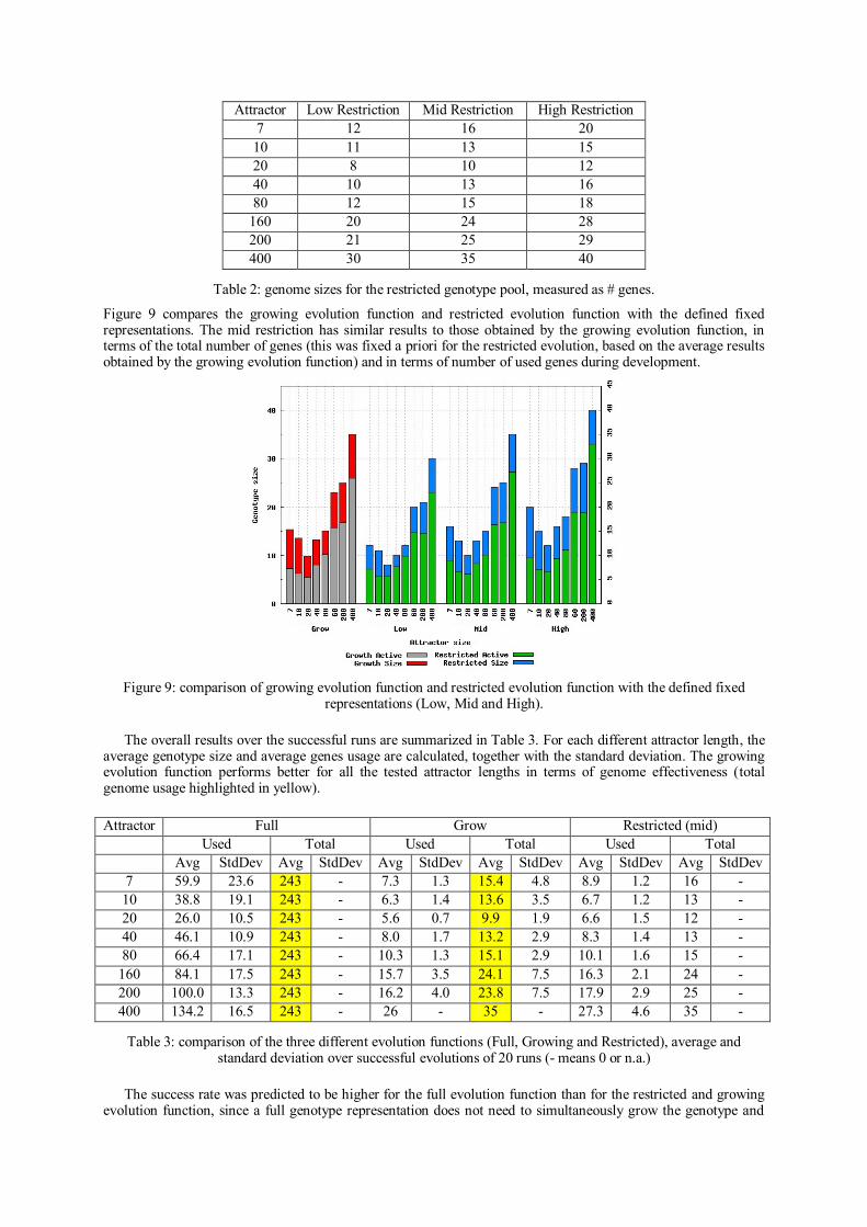
Attractor Low Restriction Mid Restriction High Restriction
7 12 16 20
10 11 13 15
20 8 10 12
40 10 13 16
80 12 15 18
160 20 24 28
200 21 25 29
400 30 35 40
Table 2: genome sizes for the restricted genotype pool, measured as # genes.
Figure 9 compares the growing evolution function and restricted evolution function with the defined fixed representations. The mid restriction has similar results to those obtained by the growing evolution function, in terms of the total number of genes (this was fixed a priori for the restricted evolution, based on the average results obtained by the growing evolution function) and in terms of number of used genes during development.
Figure 9: comparison of growing evolution function and restricted evolution function with the defined fixed representations (Low, Mid and High).
The overall results over the successful runs are summarized in Table 3. For each different attractor length, the average genotype size and average genes usage are calculated, together with the standard deviation. The growing evolution function performs better for all the tested attractor lengths in terms of genome effectiveness (total genome usage highlighted in yellow).
Attractor Full Grow Restricted (mid)
Used Total Used Total Used Total
Avg StdDev Avg StdDev Avg StdDev Avg StdDev Avg StdDev Avg StdDev
7 59.9 23.6 243 - 7.3 1.3 15.4 4.8 8.9 1.2 16 -
10 38.8 19.1 243 - 6.3 1.4 13.6 3.5 6.7 1.2 13 -
20 26.0 10.5 243 - 5.6 0.7 9.9 1.9 6.6 1.5 12 -
40 46.1 10.9 243 - 8.0 1.7 13.2 2.9 8.3 1.4 13 -
80 66.4 17.1 243 - 10.3 1.3 15.1 2.9 10.1 1.6 15 -
160 84.1 17.5 243 - 15.7 3.5 24.1 7.5 16.3 2.1 24 -
200 100.0 13.3 243 - 16.2 4.0 23.8 7.5 17.9 2.9 25 -
400 134.2 16.5 243 - 26 - 35 - 27.3 4.6 35 -
Table 3: comparison of the three different evolution functions (Full, Growing and Restricted), average and standard deviation over successful evolutions of 20 runs (- means 0 or n.a.)
The success rate was predicted to be higher for the full evolution function than for the restricted and growing evolution function, since a full genotype representation does not need to simultaneously grow the genotype and
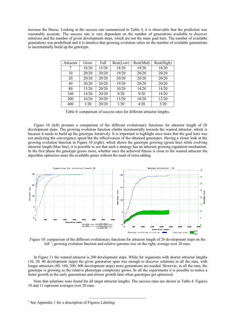
increase the fitness. Looking at the success rate summarized in Table 4, it is observable that the prediction was reasonably accurate. The success rate is very dependent on the number of generations available to discover solutions and the number of given development steps, which are not the main goal here. The number of available generations was predefined and it is intuitive that growing evolution relies on the number of available generations to incrementally build up the genotype.
Attractor Grow Full Rest(Low) Rest(Mid) Rest(High)
7 18/20 15/20 18/20 19/20 18/20
10 20/20 20/20 19/20 20/20 20/20
20 20/20 20/20 20/20 20/20 20/20
40 20/20 20/20 19/20 20/20 20/20
80 15/20 20/20 10/20 14/20 14/20
160 14/20 20/20 9/20 9/20 14/20
200 16/20 20/20 13/20 10/20 12/20
400 1/20 20/20 1/20 4/20 3/20
Table 4: comparison of success rates for different attractor lengths.
Figure 10 (left) presents a comparison of the different evolutionary functions for attractor length of 20 development steps. The growing evolution function climbs incrementally towards the wanted attractor, which is because it needs to build up the genotype iteratively. It is important to highlight once more that the goal here was not analyzing the convergence speed but the effectiveness of the obtained genotypes. Having a closer look at the growing evolution function in Figure 10 (right), which shows the genotype growing (green line) while evolving attractor length (blue line), it is possible to see that such a strategy has an inherent growing regulation mechanism. In the first phase the genotype grows more, whether once the achieved fitness is close to the wanted attractor the algorithm optimizes more the available genes without the need of extra adding.
Figure 10: comparison of the different evolutionary functions for attractor length of 20 development steps on the left 1; growing evolution function and relative genome size on the right; average over 20 runs.
In Figure 11 the wanted attractor is 200 development steps. While for organisms with shorter attractor lengths (10, 20, 40 development steps) the given generation span was enough to discover solutions in all the runs, with longer attractors (80, 160, 200, 400 development steps) more generations are needed. However, in all the runs, the genotype is growing as the relative phenotype complexity grows. In all the experiments it is possible to notice a faster growth in the early generations and slower growth later when genotypes get optimized.
Note that solutions were found for all target attractor lengths. The success rates are shown in Table 4. Figures 10 and 11 represent averages over 20 runs.
1 See Appendix 1 for a description of Figures Labeling
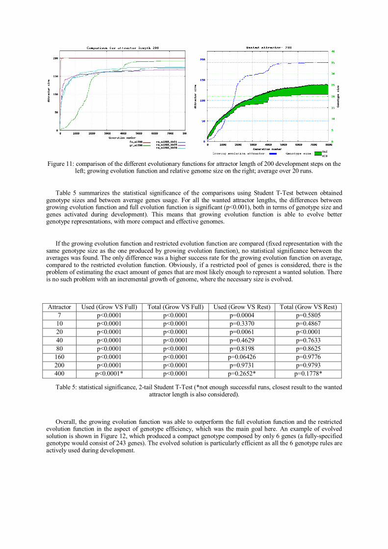
Figure 11: comparison of the different evolutionary functions for attractor length of 200 development steps on the left; growing evolution function and relative genome size on the right; average over 20 runs.
Table 5 summarizes the statistical significance of the comparisons using Student T-Test between obtained genotype sizes and between average genes usage. For all the wanted attractor lengths, the differences between growing evolution function and full evolution function is significant (p<0.001), both in terms of genotype size and genes activated during development). This means that growing evolution function is able to evolve better genotype representations, with more compact and effective genomes.
If the growing evolution function and restricted evolution function are compared (fixed representation with the same genotype size as the one produced by growing evolution function), no statistical significance between the averages was found. The only difference was a higher success rate for the growing evolution function on average, compared to the restricted evolution function. Obviously, if a restricted pool of genes is considered, there is the problem of estimating the exact amount of genes that are most likely enough to represent a wanted solution. There is no such problem with an incremental growth of genome, where the necessary size is evolved.
Attractor Used (Grow VS Full) Total (Grow VS Full) Used (Grow VS Rest) Total (Grow VS Rest)
7 p<0.0001 p<0.0001 p=0.0004 p=0.5805
10 p<0.0001 p<0.0001 p=0.3370 p=0.4867
20 p<0.0001 p<0.0001 p=0.0061 p<0.0001
40 p<0.0001 p<0.0001 p=0.4629 p=0.7633
80 p<0.0001 p<0.0001 p=0.8198 p=0.8625
160 p<0.0001 p<0.0001 p=0.06426 p=0.9776
200 p<0.0001 p<0.0001 p=0.9731 p=0.9793
400 p<0.0001* p<0.0001 p=0.2652* p=0.1778*
Table 5: statistical significance, 2-tail Student T-Test (*not enough successful runs, closest result to the wanted attractor length is also considered).
Overall, the growing evolution function was able to outperform the full evolution function and the restricted evolution function in the aspect of genotype efficiency, which was the main goal here. An example of evolved solution is shown in Figure 12, which produced a compact genotype composed by only 6 genes (a fully-specified genotype would consist of 243 genes). The evolved solution is particularly efficient as all the 6 genotype rules are actively used during development.
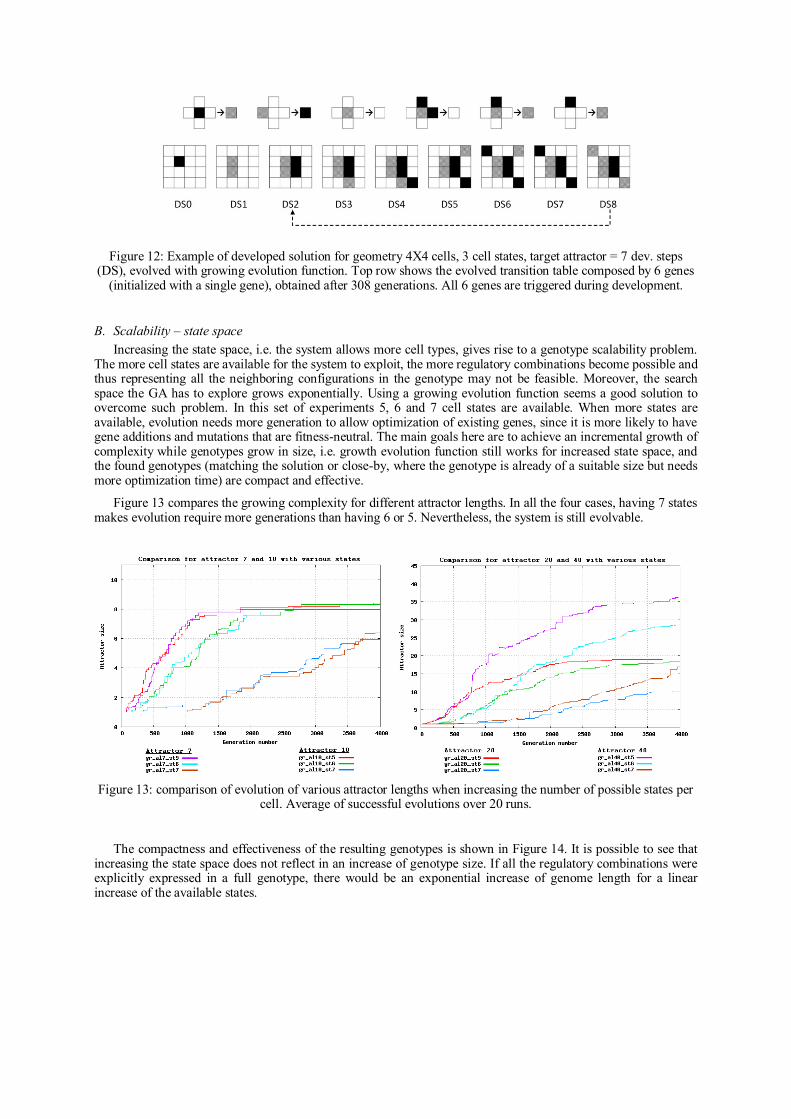
Figure 12: Example of developed solution for geometry 4X4 cells, 3 cell states, target attractor = 7 dev. steps
(DS), evolved with growing evolution function. Top row shows the evolved transition table composed by 6 genes (initialized with a single gene), obtained after 308 generations. All 6 genes are triggered during development.
B. Scalability – state space
Increasing the state space, i.e. the system allows more cell types, gives rise to a genotype scalability problem. The more cell states are available for the system to exploit, the more regulatory combinations become possible and thus representing all the neighboring configurations in the genotype may not be feasible. Moreover, the search space the GA has to explore grows exponentially. Using a growing evolution function seems a good solution to overcome such problem. In this set of experiments 5, 6 and 7 cell states are available. When more states are available, evolution needs more generation to allow optimization of existing genes, since it is more likely to have gene additions and mutations that are fitness-neutral. The main goals here are to achieve an incremental growth of complexity while genotypes grow in size, i.e. growth evolution function still works for increased state space, and the found genotypes (matching the solution or close-by, where the genotype is already of a suitable size but needs more optimization time) are compact and effective.
Figure 13 compares the growing complexity for different attractor lengths. In all the four cases, having 7 states makes evolution require more generations than having 6 or 5. Nevertheless, the system is still evolvable.
Figure 13: comparison of evolution of various attractor lengths when increasing the number of possible states per cell. Average of successful evolutions over 20 runs.
The compactness and effectiveness of the resulting genotypes is shown in Figure 14. It is possible to see that increasing the state space does not reflect in an increase of genotype size. If all the regulatory combinations were explicitly expressed in a full genotype, there would be an exponential increase of genome length for a linear increase of the available states.
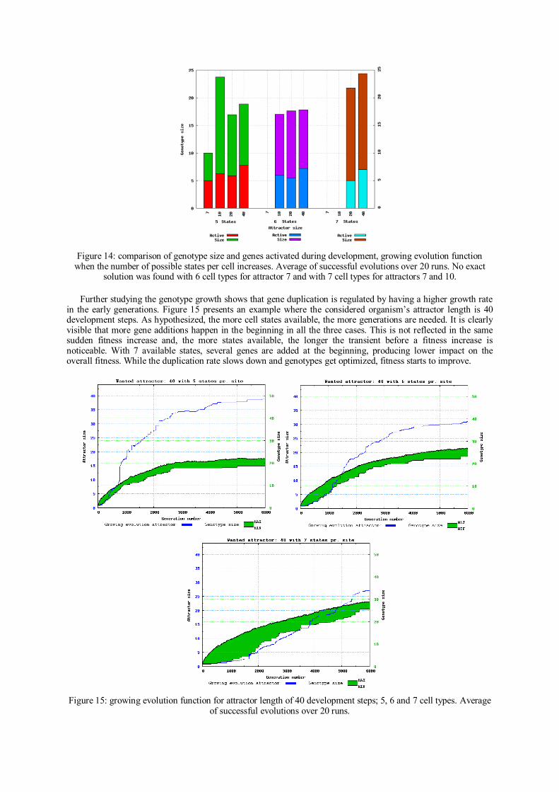
Figure 14: comparison of genotype size and genes activated during development, growing evolution function when the number of possible states per cell increases. Average of successful evolutions over 20 runs. No exact
solution was found with 6 cell types for attractor 7 and with 7 cell types for attractors 7 and 10.
Further studying the genotype growth shows that gene duplication is regulated by having a higher growth rate in the early generations. Figure 15 presents an example where the considered organism’s attractor length is 40 development steps. As hypothesized, the more cell states available, the more generations are needed. It is clearly visible that more gene additions happen in the beginning in all the three cases. This is not reflected in the same sudden fitness increase and, the more states available, the longer the transient before a fitness increase is noticeable. With 7 available states, several genes are added at the beginning, producing lower impact on the overall fitness. While the duplication rate slows down and genotypes get optimized, fitness starts to improve.
Figure 15: growing evolution function for attractor length of 40 development steps; 5, 6 and 7 cell types. Average of successful evolutions over 20 runs.
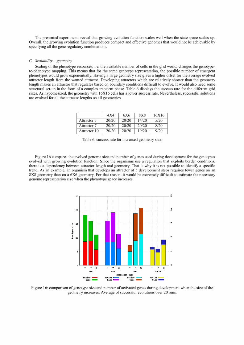
The presented experiments reveal that growing evolution function scales well when the state space scales-up. Overall, the growing evolution function produces compact and effective genomes that would not be achievable by specifying all the gene regulatory combinations.
C. Scalability – geometry
Scaling of the phenotype resources, i.e. the available number of cells in the grid world, changes the genotype-to-phenotype mapping. This means that for the same genotype representation, the possible number of emergent phenotypes would grow exponentially. Having a large geometry size gives a higher offset for the average evolved attractor length from the wanted attractor. Developing attractors which are relatively shorter than the geometry length makes an attractor that regulates based on boundary conditions difficult to evolve. It would also need some structural set-up in the form of a complex transient phase. Table 6 displays the success rate for the different grid sizes. As hypothesized, the geometry with 16X16 cells has a lower success rate. Nevertheless, successful solutions are evolved for all the attractor lengths on all geometries.
4X4 6X6 8X8 16X16
Attractor 5 20/20 20/20 14/20 5/20
Attractor 7 20/20 20/20 20/20 8/20
Attractor 10 20/20 20/20 19/20 9/20
Table 6: success rate for increased geometry size.
Figure 16 compares the evolved genome size and number of genes used during development for the genotypes evolved with growing evolution function. Since the organisms use a regulation that exploits border conditions, there is a dependency between attractor length and geometry. That is why it is not possible to identify a specific trend. As an example, an organism that develops an attractor of 5 development steps requires fewer genes on an 8X8 geometry than on a 6X6 geometry. For that reason, it would be extremely difficult to estimate the necessary genome representation size when the phenotype space increases.
Figure 16: comparison of genotype size and number of activated genes during development when the size of the geometry increases. Average of successful evolutions over 20 runs.
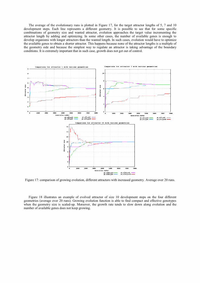
The average of the evolutionary runs is plotted in Figure 17, for the target attractor lengths of 5, 7 and 10 development steps. Each line represents a different geometry. It is possible to see that for some specific combinations of geometry size and wanted attractor, evolution approaches the target value incrementing the attractor length by adding and optimizing. In some other cases, the number of available genes is enough to develop organisms with longer attractors than the wanted length. In such cases, evolution would have to optimize the available genes to obtain a shorter attractor. This happens because none of the attractor lengths is a multiple of the geometry side and because the simplest way to regulate an attractor is taking advantage of the boundary conditions. It is extremely important that in such case, growth does not get out of control.
Figure 17: comparison of growing evolution, different attractors with increased geometry. Average over 20 runs.
Figure 18 illustrates an example of evolved attractor of size 10 development steps on the four different geometries (average over 20 runs). Growing evolution function is able to find compact and effective genotypes when the geometry size is scaled-up. Moreover, the growth rate tends to slow down along evolution and the number of available genes does not keep growing.
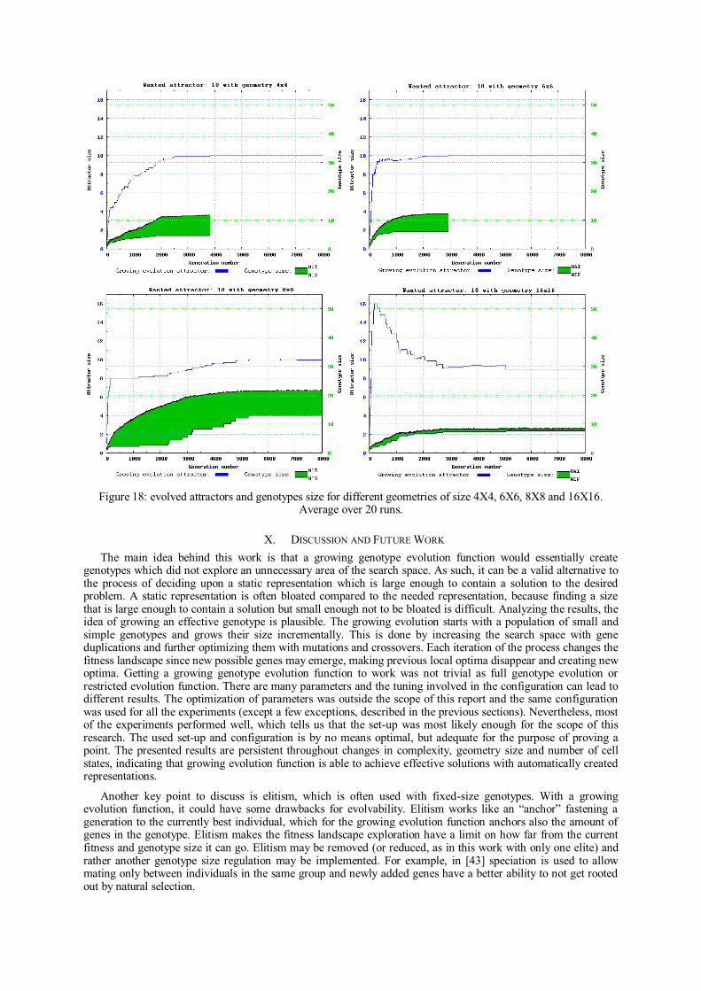
Figure 18: evolved attractors and genotypes size for different geometries of size 4X4, 6X6, 8X8 and 16X16. Average over 20 runs.
X. DISCUSSION AND FUTURE WORK
The main idea behind this work is that a growing genotype evolution function would essentially create genotypes which did not explore an unnecessary area of the search space. As such, it can be a valid alternative to the process of deciding upon a static representation which is large enough to contain a solution to the desired problem. A static representation is often bloated compared to the needed representation, because finding a size that is large enough to contain a solution but small enough not to be bloated is difficult. Analyzing the results, the idea of growing an effective genotype is plausible. The growing evolution starts with a population of small and simple genotypes and grows their size incrementally. This is done by increasing the search space with gene duplications and further optimizing them with mutations and crossovers. Each iteration of the process changes the fitness landscape since new possible genes may emerge, making previous local optima disappear and creating new optima. Getting a growing genotype evolution function to work was not trivial as full genotype evolution or restricted evolution function. There are many parameters and the tuning involved in the configuration can lead to different results. The optimization of parameters was outside the scope of this report and the same configuration was used for all the experiments (except a few exceptions, described in the previous sections). Nevertheless, most of the experiments performed well, which tells us that the set-up was most likely enough for the scope of this research. The used set-up and configuration is by no means optimal, but adequate for the purpose of proving a point. The presented results are persistent throughout changes in complexity, geometry size and number of cell states, indicating that growing evolution function is able to achieve effective solutions with automatically created representations.
Another key point to discuss is elitism, which is often used with fixed-size genotypes. With a growing evolution function, it could have some drawbacks for evolvability. Elitism works like an “anchor” fastening a generation to the currently best individual, which for the growing evolution function anchors also the amount of genes in the genotype. Elitism makes the fitness landscape exploration have a limit on how far from the current fitness and genotype size it can go. Elitism may be removed (or reduced, as in this work with only one elite) and rather another genotype size regulation may be implemented. For example, in [43] speciation is used to allow mating only between individuals in the same group and newly added genes have a better ability to not get rooted out by natural selection.
The solutions found in all the different sets of experiments are successful and the resulting genotypes are more compact and effective. Growing a genotype is a valid alternative to defining a static representation or using a full representation with all the possible regulatory combinations. Comparing the result of the growing evolution function to the restricted evolution function shows that the performances are similar. This means that the growing genomes are reasonably optimized.
An inherent result of the growing evolution function to target organisms that develop an attractor of a specific number of development steps is a rather small transient. This is consistent with other work [34], [4] where there is no instruction sequence or construction arm and the construction of structures is a fission-like process with high parallel processing.
The goal in this work was to evolve organisms which produced attractors of different lengths, instead of simply achieving a given structure. This means that the resulting solutions take advantage of geometry regulation, i.e. actively use the geometry to build structures that achieve the required attractor size. These structures have directional movement, but because of periodic boundary conditions, they cycle around the grid and return to sites that have previously occupied. This way, structures can either move at a certain speed which combined with the geometry results in an appropriate attractor or move and leave behind structures with which it can interact when cycling around the boundary, essentially creating an environment for itself to evolve within. As such, repeating patterns within an attractor may emerge. For larger geometries, having attractors that do not rely on boundary conditions would mean having a larger set of genes regulating a developing mechanism and a stopping mechanism. A kind of location fixed attractor which stays within a fixed geometric space even if the total geometry is limitless is very difficult to achieve. That is why most of the solutions take advantage of geometry regulations.
Evolutionary and Developmental Systems and Artificial Intelligence rely on efficient search of optimized structures, most likely very large structures that suffer from an inherent scalability issue. Evolutionary growth of genome representations is the tool that allows such scaling-up, starting from the very simple and incrementally elaborating. As a consequence, it may be advantageous to explore it in such domains where scalability is a goal.
As future work, it may be interesting to investigate evolutionary growth of genome representations not only in terms of search space but also in the state space. Essentially let the growth happen both in terms of genotype size, i.e. number of genes, and states that each cell can hold, i.e. number of possible cell states. This would achieve true complexification, meaning that the boundaries are not fixed by the state space (which is more or less fixed in every artificial system). This would allow systems to evolve for arbitrary complexity levels and find solutions to arbitrary complex problems.
XI. CONCLUSION
The experiments presented in this paper show that the evolutionary growth of genotype representations for EvoDevo systems with indirect encodings produces compact and effective genomes. This is without the need of fully specifying all the regulatory combinations or estimating a priori the necessary genetic pool with complex heuristics. Three types of scalability issues are discussed. (1) The scalability of the search space: the growing evolution function outperforms restricted evolution and full evolution in terms of genome size and genome exploitation by complexification of simple genotypes with the incremental addition and optimization of new genes. The result is that complexity of achieved solutions grows while evolution progresses. (2) The scalability of the state space: growing evolution function is effective when the number of available cell states is scaled-up and a fully specified genome would not be possible. (3) The scalability of phenotypic resources: developmental systems take advantage of an indirect genotype-to-phenotype mapping and scaling-up the phenotype resources increases the complexity of the mapping. The growing evolution function provides the necessary genotype scalability to elaborate solutions with compact and effective genomes when the grid world where organisms develop is increased in size.
Overall, the key aspect of evolutionary growth of genotype representations is the ability to solve difficult problems by starting with simple solutions in a low dimensional space and incrementally increasing the genotype complexity, disregarding how large a genotype would be to encode a solution. As such, it is a powerful strategy in the field of evolutionary and developmental systems with indirect encodings, where nature-like levels of complexity are targeted.
REFERENCES
[1] L. Altenberg. Genome growth and the evolution of the genotype-phenotype map. In W. Banzhaf and F. H. Eeckman, editors, Evolution
and Biocomputation, volume 899 of Lecture Notes in Computer Science, pages 205–259. Springer, 1995.
[2] W. R. Ashby. An introduction to cybernetics. Chapman & Hall, London, 1956.
[3] E. Bianconi, A. Piovesan, F. Facchin, A. Beraudi, R. Casadei, F. Frabetti, L. Vitale, M. C. Pelleri, S. Tassani, F. Piva, S. Perez-
Amodio, P. Strippoli, and S. Canaider. An estimation of the number of cells in the human body. Annals of Human Biology, 0(0):1–9, 2013. PMID: 23829164.
[4] M. Bidlo and Z. Vasicek. Evolution of cellular automata using instruction-based approach. In Evolutionary Computation (CEC), 2012
IEEE Congress on, pages 1–8, 2012.
[5] D. Cliff, P. Husbands, and I. Harvey. Explorations in evolutionary robotics. Adaptive Behaviour, 2(1):73–110, 1993.
[6] W. F. Doolittle. Uprooting the tree of life. Scientific American, (282):90–95, 2000.
[7] R. Doursat. Organically Grown Architectures: Creating Decentralized, Autonomous Systems by Embryomorphic Engineering. pages
167–199. 2008.
[8] R. Doursat, H. Sayama, and O. Michel. Morphogenetic Engineering: Toward Programmable Complex Systems. Springer Publishing
Company, Incorporated, 2013.
[9] D. Federici and K. Downing. Evolution and development of a multicellular organism: Scalability, resilience, and neutral complexification. Artificial Life, 12:2006, 2006.
[10] A. Giskeødegård. Inkrementell vekst av genomet for evolusjon av genotype representasjoner for kunstige cellulære organismer, 2013.
[11] N. Glansdorff, Y. Xu, and B. Labedan. The last universal common ancestor: emergence, constitution and genetic legacy of an elusive
forerunner. Biology Direct, 3(1):1–35, 2008.
[12] B. K. Hall, R. D. Pearson, and G. B. Müller. Environment, development, and evolution: toward a synthesis. The Vienna Series in Theoretical Biology. MIT Press, 2004.
[13] I. Harvey, P. Husbands, and D. Cliff. Seeing the light: Artificial evolution, real vision, 1994.
[14] G. S. Hornby. Functional scalability through generative representations: the evolution of table designs. Environment and Planning B: Planning and Design, 31:569–587, 2004.
[15] H. Kitano. Designing neural networks using genetic algorithms with graph generation system. Complex Systems, 4:461–476, 1990.
[16] H. Kitano. Building complex systems using developmental process: An engineering approach. In M. Sipper, D. Mange, and A. Perez-
Uribe, editors, Evolvable Systems: From Biology to Hardware, volume 1478 of Lecture Notes in Computer Science, pages 218–229. Springer Berlin Heidelberg, 1998.
[17] T. Kowaliw. Measures of complexity for artificial embryogeny. In Proceedings of the 10th annual conference on Genetic and
evolutionary computation, GECCO ’08, pages 843–850, New York, NY, USA, 2008. ACM.
[18] T. Kowaliw and W. Banzhaf. Augmenting artificial development with local fitness. In IEEE Congress on Evolutionary Computation, pages 316–323. IEEE, 2009.
[19] T. Kowaliw, P. Grogono, and N. Kharma. Environment as a spatial constraint on the growth of structural form. In Proceedings of the
9th annual conference on Genetic and evolutionary computation, GECCO ’07, pages 1037–1044, New York, NY, USA, 2007. ACM.
[20] J. R. Koza. Gene duplication to enable genetic programming to concurrently evolve both the architecture and work-performing steps . .
. In In IJCAI-95 Proceedings of the fourteenth International Joint Conference on Artificial Intelligence, pages 734–740. Morgan Kaufmann, 1995.
[21] J. R. Koza, D. Andre, F. H. Bennett, and M. A. Keane. Genetic Programming III: Darwinian Invention & Problem Solving. Morgan
Kaufmann Publishers Inc., 1999.
[22] S. Kumar and P. J. Bentley. Biologically Inspired Evolutionary Development. Evolvable Systems: From Biology to Hardware, pages 99–106, 2003.
[23] C. G. Langton. Self-reproduction in cellular automata. Physica D, 10D(1-2):135–44, 1984.
[24] W.-H. Li, Z. Gu, H. Wang, and A. Nukrutenko. Evolutionary analyses of the human genome. Nature, (409):847–849, 2001.
[25] K. Lindgren and J. Johansson. Coevolution of strategies in n-person prisoner’s dilemma. Evolutionary Dynamics-Exploring the
Interplay of Selection, Jan. 2001.
[26] A. P. Martin. Increasing genomic complexity by gene duplication and the origin of vertebrates. The American Naturalist, 154(2):pp.
111–128, 1999.
[27] J. F. Miller and W. Banzhaf. Evolving the program for a cell: from french flags to boolean circuits. In S. Kumar and P. J. Bentley, editors, On Growth, Form and Computers. Academic Press, October 2003.
[28] J. V. Neumann. Theory of Self-Reproducing Automata. University of Illinois Press, Champaign, IL, USA, 1966.
[29] S. Nichele and G. Tufte. Trajectories and attractors as specification for the evolution of behaviour in cellular automata. In Evolutionary
Computation (CEC), 2010 IEEE Congress on, pages 1–8. IEEE, 2010.
[30] S. Nichele and G. Tufte. Genome parameters as information to forecast emergent developmental behaviors. In Unconventional Computation and Natural Computation, pages 186–197. Springer, 2012.
[31] S. Nichele and G. Tufte. Evolution of incremental complex behavior on cellular machines. In Advances in Artificial Life, ECAL,
volume 12, pages 63–70, 2013.
[32] S. Nolfi and D. Floreano. Evolutionary Robotics: The Biology,Intelligence,and Technology of Self-Organizing Machines. MIT Press,
Cambridge, MA, USA, 2000.
[33] S. Ohno. Evolution by Gene Duplication. Allen and Unwin, London, UK, 1970.
[34] Z. Pan and J. A. Reggia. Computational discovery of instructionless self-replicating structures in cellular automata. Artificial Life, 16:39–63, 2010.
[35] F. Rothlauf and D. E. Goldberg. Redundant representations in evolutionary computation. Evolutionary Computation, 11(4):381–415,
2003.
[36] L. Sekanina and M. Bidlo. Evolutionary design of arbitrarily large sorting networks using development. Genetic Programming and Evolvable Machines, 6(3):319–347, 2005.
[37] L. Sekanina and M. Bidlo. Evolutionary design of arbitrarily large sorting networks using development. Genetic Programming and
Evolvable Machines, 6(3):319–347, 2005.
[38] M. Shackleton, R. Shipman, and M. Ebner. An investigation of redundant genotype-phenotype mappings and their role in evolutionary
search. In Evolutionary Computation, 2000. Proceedings of the 2000 Congress on, pages 493–500. IEEE, 2000.
[39] R. Shipman. Genetic redundancy: desirable or problematic for evolutionary adaptation? In Artificial Neural Nets and Genetic Algorithms, 1999. Proceedings of the International Conference on, pages 337–344. Springer-Verlag, 1999.
[40] R. Shipman, M. Shackleton, M. Ebner, and R. Watson. Neutral search spaces for artificial evolution: a lesson from life. In Artificial
Life VII, Proceedings of the Seventh International Conference on Artificial Life, pages 162–169. MIT Press, 2000.
[41] K. O. Stanley and R. Miikkulainen. Achieving high-level functionality through evolutionary complexification. In Proceedings of the AAAI-2003 Spring Symposium on Computational Synthesis, Stanford, CA, 2003. AAAI Press.
[42] K. O. Stanley and R. Miikkulainen. A taxonomy for artificial embryogeny. Artificial Life, 9(2):93–130, 2003.
[43] K. O. Stanley and R. Miikkulainen. Competitive coevolution through evolutionary complexification. Journal of Artificial Intelligence
Research, 21:63–100, 2004.
[44] M. Steel and D. Penny. Origins of life: Common ancestry put to the test. Nature, (7295):168–9, 2010.
[45] J. S. Taylor and J. Raes. Duplication and divergence: The evolution of new genes and old ideas. Annual Review of Genetics, 38(1):615–
643, 2004. PMID: 15568988.
[46] D. L. Theobald. A formal test of the theory of universal common ancestry. Nature, (7295):219–222, 2010.
[47] G. Tufte. Discovery and investigation of inherent scalability in developmental genomes. In G. Hornby, L. Sekanina, and P. C. Haddow, editors, ICES, volume 5216 of Lecture Notes in Computer Science, pages 189–200. Springer, 2008.
[48] G. Tufte. Evolution, development and environment toward adaptation through phenotypic plasticity and exploitation of external
information. In R. W. M. B. Seth Bullock (Chair), Jason Noble, editor, Artificial Life XI (ALIFE XI). MIT Press, 2008.
[49] G. Tufte. Phenotypic, developmental and computational resources: Scaling in artificial development. In Genetic and Evolutionary Computation (GECCO , 2008). ACM, 2008.
[50] G. Tufte and S. Nichele. On the correlations between developmental diversity and genomic composition. In Proceedings of the 13th
annual conference on Genetic and evolutionary computation, pages 1507–1514. ACM, 2011.
[51] G. Tufte and J. Thomassen. Size matters: Scaling of organism and genomes for development of emergent structures. In Genetic and
Evolutionary Computation (GECCO), ACM conference series. ACM, 2006.
[52] J. C. Venter, M. D. Adams, E. W. Myers, P. W. Li, R. J. Mural, G. G. Sutton, H. O. Smith, M. Yandell, C. A. Evans, R. A. Holt, J. D. Gocayne, P. Amanatides, R. M. Ballew, D. H. Huson, J. R. Wortman, Q. Zhang, C. D. Kodira, X. H. Zheng, L. Chen, M. Skupski,
G. Subramanian, P. D. Thomas, J. Zhang, G. L. Gabor Miklos, C. Nelson, S. Broder, A. G. Clark, J. Nadeau, V. A. McKusick, N. Zinder, A. J. Levine, R. J. Roberts, M. Simon, C. Slayman, M. Hunkapiller, R. Bolanos, A. Delcher, I. Dew, D. Fasulo, M. Flanigan,
L. Florea, A. Halpern, S. Hannenhalli, S. Kravitz, S. Levy, C. Mobarry, K. Reinert, K. Remington, J. Abu-Threideh, E. Beasley, K. Biddick, V. Bonazzi, R. Brandon, M. Cargill, I. Chandramouliswaran, R. Charlab, K. Chaturvedi, Z. Deng, V. D. Francesco,
P. Dunn, K. Eilbeck, C. Evangelista, A. E. Gabrielian, W. Gan, W. Ge, F. Gong, Z. Gu, P. Guan, T. J. Heiman, M. E. Higgins, R.-R. Ji, Z. Ke, K. A. Ketchum, Z. Lai, Y. Lei, Z. Li, J. Li, Y. Liang, X. Lin, F. Lu, G. V. Merkulov, N. Milshina, H. M. Moore, A. K. Naik,
V. A. Narayan, B. Neelam, D. Nusskern, D. B. Rusch, S. Salzberg, W. Shao, B. Shue, J. Sun, Z. Y. Wang, A. Wang, X. Wang, J. Wang, M.-H. Wei, R. Wides, C. Xiao, C. Yan, A. Yao, J. Ye, M. Zhan, W. Zhang, H. Zhang, Q. Zhao, L. Zheng, F. Zhong,
W. Zhong, S. C. Zhu, S. Zhao, D. Gilbert, S. Baumhueter, G. Spier, C. Carter, A. Cravchik, T. Woodage, F. Ali, H. An, A. Awe, D. Baldwin, H. Baden, M. Barnstead, I. Barrow, K. Beeson, D. Busam, A. Carver, A. Center, M. L. Cheng, L. Curry, S. Danaher,
L. Davenport, R. Desilets, S. Dietz, K. Dodson, L. Doup, S. Ferriera, N. Garg, A. Gluecksmann, B. Hart, J. Haynes, C. Haynes, C. Heiner, S. Hladun, D. Hostin, J. Houck, T. Howland, C. Ibegwam, J. Johnson, F. Kalush, L. Kline, S. Koduru, A. Love, F. Mann,
D. May, S. McCawley, T. McIntosh, I. McMullen, M. Moy, L. Moy, B. Murphy, K. Nelson, C. Pfannkoch, E. Pratts, V. Puri, H. Qureshi, M. Reardon, R. Rodriguez, Y.-H. Rogers, D. Romblad, B. Ruhfel, R. Scott, C. Sitter, M. Smallwood, E. Stewart, R. Strong,
E. Suh, R. Thomas, N. N. Tint, S. Tse, C. Vech, G. Wang, J. Wetter, S. Williams, M. Williams, S. Windsor, E. Winn-Deen, K. Wolfe, J. Zaveri, K. Zaveri, J. F. Abril, R. Guigó, M. J. Campbell, K. V. Sjolander, B. Karlak, A. Kejariwal, H. Mi, B. Lazareva, T. Hatton,
A. Narechania, K. Diemer, A. Muruganujan, N. Guo, S. Sato, V. Bafna, S. Istrail, R. Lippert, R. Schwartz, B. Walenz, S. Yooseph, D. Allen, A. Basu, J. Baxendale, L. Blick, M. Caminha, J. Carnes-Stine, P. Caulk, Y.-H. Chiang, M. Coyne, C. Dahlke, A. D. Mays,
M. Dombroski, M. Donnelly, D. Ely, S. Esparham, C. Fosler, H. Gire, S. Glanowski, K. Glasser, A. Glodek, M. Gorokhov, K. Graham, B. Gropman, M. Harris, J. Heil, S. Henderson, J. Hoover, D. Jennings, C. Jordan, J. Jordan, J. Kasha, L. Kagan, C. Kraft, A. Levitsky,
M. Lewis, X. Liu, J. Lopez, D. Ma, W. Majoros, J. McDaniel, S. Murphy, M. Newman, T. Nguyen, N. Nguyen, M. Nodell, S. Pan, J. Peck, M. Peterson, W. Rowe, R. Sanders, J. Scott, M. Simpson, T. Smith, A. Sprague, T. Stockwell, R. Turner, E. Venter, M. Wang,
M. Wen, D. Wu, M. Wu, A. Xia, A. Zandieh, and X. Zhu. The sequence of the human genome. Science, 291(5507):1304–1351, 2001.
[53] M. J. West-Eberhard. Developmental plasticity and evolution. Oxford University Press, New York, 2003.
[54] J. Zhang. Evolution by gene duplication: an update. Trends in Ecology & Evolution, 18(6):292–298, June 2003.
APPENDIX 1 – FIGURES LABELING
This paragraph describes the labeling template and abbreviations used for the following figures: 10, 11, 13, 15,
and 17.
fu = full evolution function;
gr = growing evolution function; re = restricted evolution function (th = threshold, number of available genes in the fixed restricted
representation).
al = target attractor length
st = number of cell states
gs = geometry size (the size of the CA grid world where organisms are developed, x by x cells)
Example 1:
fu_al200 = Full evolution function, target attractor length of 200 development steps.
Example 2:
re_al20_th10 = Restricted evolution function with maximum 10 genes, target attractor of 20 dev. steps.
Example 3:
Gr_al7_st6 = growing evolution function, target attractor length of 7 dev. steps, 6 possible states per cell.
Example 4:
Gr_al10_gs16 = growing evolution function, target attractor length of 10 dev. steps, cellular automaton
geometry of 16 by 16 cells.
Paper D.2
Evolutionary Growth of Genomes for the Development
and Replication of Multicellular Organisms
with Indirect Encodings
S. Nichele and G. Tufte
International Conference on Evolvable Systems, ICES 2014, part of the IEEE
Symposium Series on Computational Intelligence, SSCI 2014
December 9 - 12, 2014
Orlando, U.S.A.

140
Evolutionary Growth of Genomes for the
Development and Replication of Multicellular
Organisms with Indirect Encoding
Stefano Nichele and Gunnar Tufte
Norwegian University of Science and Technology
Department of Computer and Information Science
Sem Selandsvei 7-9, 7491, Trondheim, Norway
{nichele, gunnart}@idi.ntnu.no
Abstract — The genomes of biological organisms are not fixed
in size. They evolved and diverged into different species
acquiring new genes and thus having different lengths. In a way,
biological genomes are the result of a self-assembly process
where more complex phenotypes could benefit by having larger
genomes in order to survive and adapt. In the artificial domain,
evolutionary and developmental systems often have static size
genomes, e.g. chosen beforehand by the system designer by trial
and error or estimated a priori with complicated heuristics. As
such, the maximum evolvable complexity is predetermined, in
contrast to open-ended evolution in nature. In this paper, we
argue that artificial genomes may also grow in size during
evolution to produce high-dimensional solutions incrementally.
We propose an evolutionary growth of genome representations
for artificial cellular organisms with indirect encodings. Genomes
start with a single gene and acquire new genes when necessary,
thus increasing the degrees of freedom and expanding the
available search-space. Cellular Automata (CA) are used as test
bed for two different problems: replication and morphogenesis.
The chosen CA encodings are a standard developmental table
and an instruction based approach. Results show that the
proposed evolutionary growth of genomes’ method is able to
produce compact and effective genomes, without the need of
specifying the full set of regulatory configurations.
Keywords — Artificial Development, Evolution, Replication,
Complexification, Cellular Automata, Instruction-based Approach.
I. INTRODUCTION
Artificial Evolutionary and Developmental (EvoDevo) systems target principles and properties that are present in natural biological systems, such as embryogenesis, self-organization, plasticity, genotype-to-phenotype mappings, and self-repair. A major challenge for EvoDevo is the development of complex morphologies and structures, potentially at natural levels of complexity [32]. Biological multi-cellular organisms made of trillions of cells grow from a single cell which holds the complete genome [3]. However, organisms of different species have genomes of different lengths. Speciation highly relied on a gene duplication mechanism [18]. In fact, in biological organisms there is a small probability that when a parental gene is copied, more than a copy may arise, i.e. gene duplication. As such, biological evolution is an incremental process that builds up genomes of increasing complexity.
In contrast, artificial systems often rely on direct one-to-one encodings, i.e. genotype-to-phenotype mapping, where the full set of genes is mapped to the phenotype entities directly. This solution has several drawbacks, for instance scaling up the phenotype resources would imply a larger genotype which would result in a larger search space. Another possibility is to open for an indirect encoding, i.e. development or generative mapping. Such mappings are a necessity when then number of phonotype entities is large [33]. However, the scalability of such systems is still an open challenge. In fact, for several developmental systems [20, 37], it would not be possible to represent all the possible regulatory combinations in the genotype. The system designer would need to make assumption or use complex heuristic to find out a reasonable genome size, such that it would be large enough to contain a potential solution [5, 37, 38].
In this paper, we propose a biologically inspired evolutionary growth of genomes with indirect encoding, which does not rely on any a priori knowledge on the problem complexity or required genome size. Genotypes are initialized with a single gene and genotype size is incrementally evolved by means of gene duplications. This would guarantee a low dimensionality of the search space that would, in turn, evolve increasingly complex solutions and add newly created degrees of freedom only when needed. The proposed framework is tested on two different problems: the development of given patterns starting from an initial seed [9] and the replication of cellular structures [15]. Self-replication allows reuse of genetic material, reducing genome size and enabling the production of complex structures.
Related work was done towards achieving genome size expansion [6, 12, 14, 17] with variable length genomes, mostly using direct encodings [10, 34]. Research on complexification with direct encodings may not be conclusive but the idea of incremental evolutionary growth of genomes has a potential for exploration with indirect encodings [32]. With direct encodings, a variable length genome allows to duplicate a gene that is mapped to a single phenotypic entity. This would result in a duplication of the correspondent phenotypic structure itself. Such approach has been shown to be particularly successful when modular structures ought to be evolved [7]. In contrast, with indirect encodings, adding a new gene may have
978-1-4799-4479-8/14/$31.00 ©2014 IEEE 141
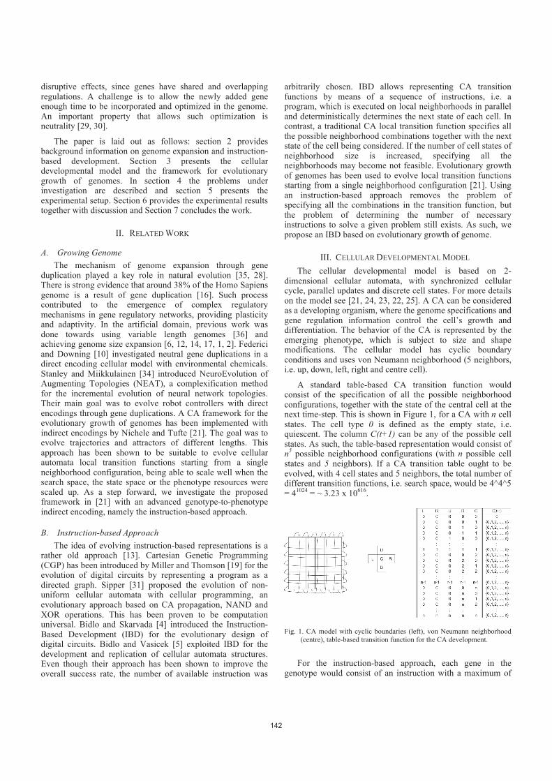
disruptive effects, since genes have shared and overlapping regulations. A challenge is to allow the newly added gene enough time to be incorporated and optimized in the genome. An important property that allows such optimization is neutrality [29, 30].
The paper is laid out as follows: section 2 provides background information on genome expansion and instruction-based development. Section 3 presents the cellular developmental model and the framework for evolutionary growth of genomes. In section 4 the problems under investigation are described and section 5 presents the experimental setup. Section 6 provides the experimental results together with discussion and Section 7 concludes the work.
II. RELATED WORK
A. Growing Genome
The mechanism of genome expansion through gene duplication played a key role in natural evolution [35, 28]. There is strong evidence that around 38% of the Homo Sapiens genome is a result of gene duplication [16]. Such process contributed to the emergence of complex regulatory mechanisms in gene regulatory networks, providing plasticity and adaptivity. In the artificial domain, previous work was done towards using variable length genomes [36] and achieving genome size expansion [6, 12, 14, 17, 1, 2]. Federici and Downing [10] investigated neutral gene duplications in a direct encoding cellular model with environmental chemicals. Stanley and Miikkulainen [34] introduced NeuroEvolution of Augmenting Topologies (NEAT), a complexification method for the incremental evolution of neural network topologies. Their main goal was to evolve robot controllers with direct encodings through gene duplications. A CA framework for the evolutionary growth of genomes has been implemented with indirect encodings by Nichele and Tufte [21]. The goal was to evolve trajectories and attractors of different lengths. This approach has been shown to be suitable to evolve cellular automata local transition functions starting from a single neighborhood configuration, being able to scale well when the search space, the state space or the phenotype resources were scaled up. As a step forward, we investigate the proposed framework in [21] with an advanced genotype-to-phenotype indirect encoding, namely the instruction-based approach.
B. Instruction-based Approach
The idea of evolving instruction-based representations is a rather old approach [13]. Cartesian Genetic Programming (CGP) has been introduced by Miller and Thomson [19] for the evolution of digital circuits by representing a program as a directed graph. Sipper [31] proposed the evolution of non-uniform cellular automata with cellular programming, an evolutionary approach based on CA propagation, NAND and XOR operations. This has been proven to be computation universal. Bidlo and Skarvada [4] introduced the Instruction-Based Development (IBD) for the evolutionary design of digital circuits. Bidlo and Vasicek [5] exploited IBD for the development and replication of cellular automata structures. Even though their approach has been shown to improve the overall success rate, the number of available instruction was
arbitrarily chosen. IBD allows representing CA transition functions by means of a sequence of instructions, i.e. a program, which is executed on local neighborhoods in parallel and deterministically determines the next state of each cell. In contrast, a traditional CA local transition function specifies all the possible neighborhood combinations together with the next state of the cell being considered. If the number of cell states of neighborhood size is increased, specifying all the neighborhoods may become not feasible. Evolutionary growth of genomes has been used to evolve local transition functions starting from a single neighborhood configuration [21]. Using an instruction-based approach removes the problem of specifying all the combinations in the transition function, but the problem of determining the number of necessary instructions to solve a given problem still exists. As such, we propose an IBD based on evolutionary growth of genome.
III. CELLULAR DEVELOPMENTAL MODEL
The cellular developmental model is based on 2-dimensional cellular automata, with synchronized cellular cycle, parallel updates and discrete cell states. For more details on the model see [21, 24, 23, 22, 25]. A CA can be considered as a developing organism, where the genome specifications and gene regulation information control the cell’s growth and differentiation. The behavior of the CA is represented by the emerging phenotype, which is subject to size and shape modifications. The cellular model has cyclic boundary conditions and uses von Neumann neighborhood (5 neighbors, i.e. up, down, left, right and centre cell).
A standard table-based CA transition function would consist of the specification of all the possible neighborhood configurations, together with the state of the central cell at the next time-step. This is shown in Figure 1, for a CA with n cell states. The cell type 0 is defined as the empty state, i.e. quiescent. The column C(t+1) can be any of the possible cell states. As such, the table-based representation would consist of n
5 possible neighborhood configurations (with n possible cell
states and 5 neighbors). If a CA transition table ought to be evolved, with 4 cell states and 5 neighbors, the total number of different transition functions, i.e. search space, would be 4^4^5 = 4
1024 = ~ 3.23 x 10
616.
Fig. 1. CA model with cyclic boundaries (left), von Neumann neighborhood
(centre), table-based transition function for the CA development.
For the instruction-based approach, each gene in the genotype would consist of an instruction with a maximum of
142
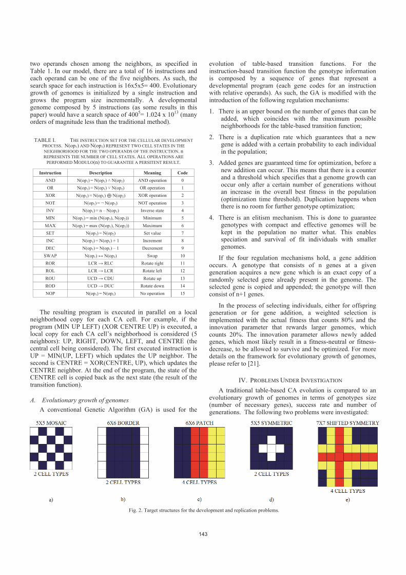
Fig. 2. Target structures for the development and replication problems.
two operands chosen among the neighbors, as specified in Table 1. In our model, there are a total of 16 instructions and each operand can be one of the five neighbors. As such, the search space for each instruction is 16x5x5= 400. Evolutionary growth of genomes is initialized by a single instruction and grows the program size incrementally. A developmental genome composed by 5 instructions (as some results in this paper) would have a search space of 400
5= 1.024 x 10
13 (many
orders of magnitude less than the traditional method).
TABLE I. THE INSTRUCTION SET FOR THE CELLULAR DEVELOPMENT
PROCESS. N(op1) AND N(op2) REPRESENT TWO CELL STATES IN THE
NEIGHBORHOOD FOR THE TWO OPERANDS OF THE INSTRUCTION. n
REPRESENTS THE NUMBER OF CELL STATES. ALL OPERATIONS ARE
PERFORMED MODULO(n) TO GUARANTEE A PERSITENT RESULT.
Instruction Description Meaning Code
AND N(op1) = N(op1) ˄ N(op2) AND operation 0
OR N(op1) = N(op1) ˅ N(op2) OR operation 1
XOR N(op1) = N(op1) ! N(op2) XOR operation 2
NOT N(op1) = ¬ N(op1) NOT operation 3
INV N(op1) = n – N(op1) Inverse state 4
MIN N(op1) = min (N(op1), N(op2)) Minimum 5
MAX N(op1) = max (N(op1), N(op2)) Maximum 6
SET N(op1) = N(op2) Set value 7
INC N(op1) = N(op1) + 1 Increment 8
DEC N(op1) = N(op1) – 1 Decrement 9
SWAP N(op1) ↔ N(op2) Swap 10
ROR LCR → RLC Rotate right 11
ROL LCR → LCR Rotate left 12
ROU UCD → CDU Rotate up 13
ROD UCD → DUC Rotate down 14
NOP N(op1) = N(op1) No operation 15
The resulting program is executed in parallel on a local neighborhood copy for each CA cell. For example, if the program (MIN UP LEFT) (XOR CENTRE UP) is executed, a local copy for each CA cell’s neighborhood is considered (5 neighbors): UP, RIGHT, DOWN, LEFT, and CENTRE (the central cell being considered). The first executed instruction is UP = MIN(UP, LEFT) which updates the UP neighbor. The second is CENTRE = XOR(CENTRE, UP), which updates the CENTRE neighbor. At the end of the program, the state of the CENTRE cell is copied back as the next state (the result of the transition function).
A. Evolutionary growth of genomes
A conventional Genetic Algorithm (GA) is used for the
evolution of table-based transition functions. For the instruction-based transition function the genotype information is composed by a sequence of genes that represent a developmental program (each gene codes for an instruction with relative operands). As such, the GA is modified with the introduction of the following regulation mechanisms:
1. There is an upper bound on the number of genes that can be added, which coincides with the maximum possible neighborhoods for the table-based transition function;
2. There is a duplication rate which guarantees that a new gene is added with a certain probability to each individual in the population;
3. Added genes are guaranteed time for optimization, before a new addition can occur. This means that there is a counter and a threshold which specifies that a genome growth can occur only after a certain number of generations without an increase in the overall best fitness in the population (optimization time threshold). Duplication happens when there is no room for further genotype optimization;
4. There is an elitism mechanism. This is done to guarantee genotypes with compact and effective genomes will be kept in the population no matter what. This enables speciation and survival of fit individuals with smaller genomes.
If the four regulation mechanisms hold, a gene addition occurs. A genotype that consists of n genes at a given generation acquires a new gene which is an exact copy of a randomly selected gene already present in the genome. The selected gene is copied and appended; the genotype will then consist of n+1 genes.
In the process of selecting individuals, either for offspring generation or for gene addition, a weighted selection is implemented with the actual fitness that counts 80% and the innovation parameter that rewards larger genomes, which counts 20%. The innovation parameter allows newly added genes, which most likely result in a fitness-neutral or fitness-decrease, to be allowed to survive and be optimized. For more details on the framework for evolutionary growth of genomes, please refer to [21].
IV. PROBLEMS UNDER INVESTIGATION
A traditional table-based CA evolution is compared to an evolutionary growth of genomes in terms of genotypes size (number of necessary genes), success rate and number of generations. The following two problems were investigated:
143
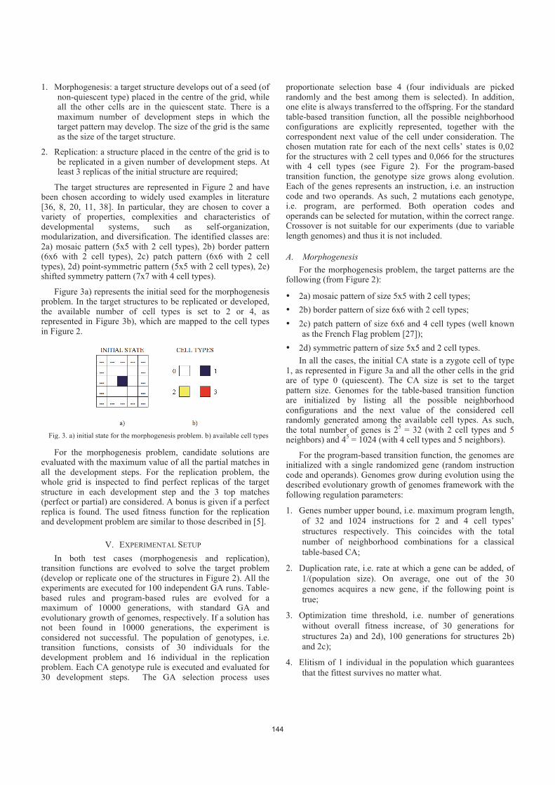
1. Morphogenesis: a target structure develops out of a seed (of non-quiescent type) placed in the centre of the grid, while all the other cells are in the quiescent state. There is a maximum number of development steps in which the target pattern may develop. The size of the grid is the same as the size of the target structure.
2. Replication: a structure placed in the centre of the grid is to be replicated in a given number of development steps. At least 3 replicas of the initial structure are required;
The target structures are represented in Figure 2 and have been chosen according to widely used examples in literature [36, 8, 20, 11, 38]. In particular, they are chosen to cover a variety of properties, complexities and characteristics of developmental systems, such as self-organization, modularization, and diversification. The identified classes are: 2a) mosaic pattern (5x5 with 2 cell types), 2b) border pattern (6x6 with 2 cell types), 2c) patch pattern (6x6 with 2 cell types), 2d) point-symmetric pattern (5x5 with 2 cell types), 2e) shifted symmetry pattern (7x7 with 4 cell types).
Figure 3a) represents the initial seed for the morphogenesis problem. In the target structures to be replicated or developed, the available number of cell types is set to 2 or 4, as represented in Figure 3b), which are mapped to the cell types in Figure 2.
For the morphogenesis problem, candidate solutions are evaluated with the maximum value of all the partial matches in all the development steps. For the replication problem, the whole grid is inspected to find perfect replicas of the target structure in each development step and the 3 top matches (perfect or partial) are considered. A bonus is given if a perfect replica is found. The used fitness function for the replication and development problem are similar to those described in [5].
V. EXPERIMENTAL SETUP
In both test cases (morphogenesis and replication), transition functions are evolved to solve the target problem (develop or replicate one of the structures in Figure 2). All the experiments are executed for 100 independent GA runs. Table-based rules and program-based rules are evolved for a maximum of 10000 generations, with standard GA and evolutionary growth of genomes, respectively. If a solution has not been found in 10000 generations, the experiment is considered not successful. The population of genotypes, i.e. transition functions, consists of 30 individuals for the development problem and 16 individual in the replication problem. Each CA genotype rule is executed and evaluated for 30 development steps. The GA selection process uses
proportionate selection base 4 (four individuals are picked randomly and the best among them is selected). In addition, one elite is always transferred to the offspring. For the standard table-based transition function, all the possible neighborhood configurations are explicitly represented, together with the correspondent next value of the cell under consideration. The chosen mutation rate for each of the next cells’ states is 0,02 for the structures with 2 cell types and 0,066 for the structures with 4 cell types (see Figure 2). For the program-based transition function, the genotype size grows along evolution. Each of the genes represents an instruction, i.e. an instruction code and two operands. As such, 2 mutations each genotype, i.e. program, are performed. Both operation codes and operands can be selected for mutation, within the correct range. Crossover is not suitable for our experiments (due to variable length genomes) and thus it is not included.
A. Morphogenesis
For the morphogenesis problem, the target patterns are the following (from Figure 2):
• 2a) mosaic pattern of size 5x5 with 2 cell types;
• 2b) border pattern of size 6x6 with 2 cell types;
• 2c) patch pattern of size 6x6 and 4 cell types (well known
as the French Flag problem [27]);
• 2d) symmetric pattern of size 5x5 and 2 cell types.
In all the cases, the initial CA state is a zygote cell of type 1, as represented in Figure 3a and all the other cells in the grid are of type 0 (quiescent). The CA size is set to the target pattern size. Genomes for the table-based transition function are initialized by listing all the possible neighborhood configurations and the next value of the considered cell randomly generated among the available cell types. As such, the total number of genes is 2
5 = 32 (with 2 cell types and 5
neighbors) and 45 = 1024 (with 4 cell types and 5 neighbors).
For the program-based transition function, the genomes are initialized with a single randomized gene (random instruction code and operands). Genomes grow during evolution using the described evolutionary growth of genomes framework with the following regulation parameters:
1. Genes number upper bound, i.e. maximum program length,
of 32 and 1024 instructions for 2 and 4 cell types’
structures respectively. This coincides with the total
number of neighborhood combinations for a classical
table-based CA;
2. Duplication rate, i.e. rate at which a gene can be added, of
1/(population size). On average, one out of the 30
genomes acquires a new gene, if the following point is
true;
3. Optimization time threshold, i.e. number of generations
without overall fitness increase, of 30 generations for
structures 2a) and 2d), 100 generations for structures 2b)
and 2c);
4. Elitism of 1 individual in the population which guarantees
that the fittest survives no matter what.
Fig. 3. a) initial state for the morphogenesis problem. b) available cell types
144
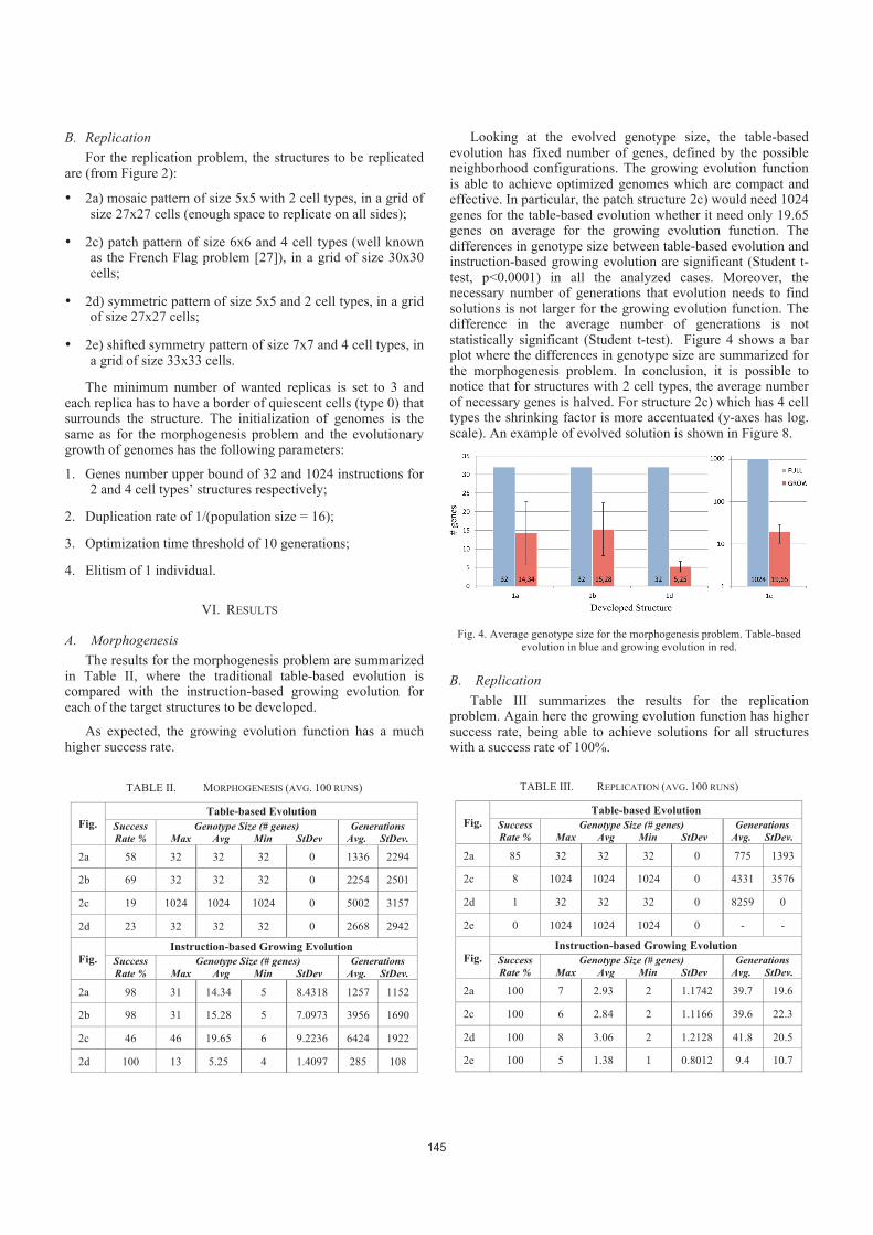
B. Replication
For the replication problem, the structures to be replicated are (from Figure 2):
• 2a) mosaic pattern of size 5x5 with 2 cell types, in a grid of size 27x27 cells (enough space to replicate on all sides);
• 2c) patch pattern of size 6x6 and 4 cell types (well known as the French Flag problem [27]), in a grid of size 30x30 cells;
• 2d) symmetric pattern of size 5x5 and 2 cell types, in a grid of size 27x27 cells;
• 2e) shifted symmetry pattern of size 7x7 and 4 cell types, in a grid of size 33x33 cells.
The minimum number of wanted replicas is set to 3 and each replica has to have a border of quiescent cells (type 0) that surrounds the structure. The initialization of genomes is the same as for the morphogenesis problem and the evolutionary growth of genomes has the following parameters:
1. Genes number upper bound of 32 and 1024 instructions for 2 and 4 cell types’ structures respectively;
2. Duplication rate of 1/(population size = 16);
3. Optimization time threshold of 10 generations;
4. Elitism of 1 individual.
VI. RESULTS
A. Morphogenesis
The results for the morphogenesis problem are summarized in Table II, where the traditional table-based evolution is compared with the instruction-based growing evolution for each of the target structures to be developed.
As expected, the growing evolution function has a much higher success rate.
TABLE II. MORPHOGENESIS (AVG. 100 RUNS)
Fig.
Table-based Evolution
Success
Rate %
Genotype Size (# genes)
Max Avg Min StDev
Generations
Avg. StDev.
2a 58 32 32 32 0 1336 2294
2b 69 32 32 32 0 2254 2501
2c 19 1024 1024 1024 0 5002 3157
2d 23 32 32 32 0 2668 2942
Fig.
Instruction-based Growing Evolution
Success
Rate %
Genotype Size (# genes)
Max Avg Min StDev
Generations
Avg. StDev.
2a 98 31 14.34 5 8.4318 1257 1152
2b 98 31 15.28 5 7.0973 3956 1690
2c 46 46 19.65 6 9.2236 6424 1922
2d 100 13 5.25 4 1.4097 285 108
Looking at the evolved genotype size, the table-based evolution has fixed number of genes, defined by the possible neighborhood configurations. The growing evolution function is able to achieve optimized genomes which are compact and effective. In particular, the patch structure 2c) would need 1024 genes for the table-based evolution whether it need only 19.65 genes on average for the growing evolution function. The differences in genotype size between table-based evolution and instruction-based growing evolution are significant (Student t-test, p<0.0001) in all the analyzed cases. Moreover, the necessary number of generations that evolution needs to find solutions is not larger for the growing evolution function. The difference in the average number of generations is not statistically significant (Student t-test). Figure 4 shows a bar plot where the differences in genotype size are summarized for the morphogenesis problem. In conclusion, it is possible to notice that for structures with 2 cell types, the average number of necessary genes is halved. For structure 2c) which has 4 cell types the shrinking factor is more accentuated (y-axes has log. scale). An example of evolved solution is shown in Figure 8.
Fig. 4. Average genotype size for the morphogenesis problem. Table-based
evolution in blue and growing evolution in red.
B. Replication
Table III summarizes the results for the replication problem. Again here the growing evolution function has higher success rate, being able to achieve solutions for all structures with a success rate of 100%.
TABLE III. REPLICATION (AVG. 100 RUNS)
Fig.
Table-based Evolution
Success
Rate %
Genotype Size (# genes)
Max Avg Min StDev
Generations
Avg. StDev.
2a 85 32 32 32 0 775 1393
2c 8 1024 1024 1024 0 4331 3576
2d 1 32 32 32 0 8259 0
2e 0 1024 1024 1024 0 - -
Fig.
Instruction-based Growing Evolution
Success
Rate %
Genotype Size (# genes)
Max Avg Min StDev
Generations
Avg. StDev.
2a 100 7 2.93 2 1.1742 39.7 19.6
2c 100 6 2.84 2 1.1166 39.6 22.3
2d 100 8 3.06 2 1.2128 41.8 20.5
2e 100 5 1.38 1 0.8012 9.4 10.7
145
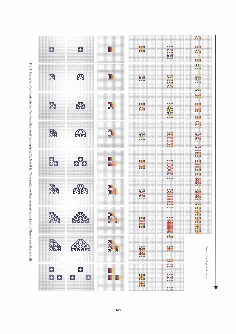
Tim
e, Dev
elop
men
t Step
s
Fig
. 5. E
xam
ples o
f evo
lved
solu
tion
s for th
e replicatio
n o
f the stru
ctures 2
d, 2
c and
2e. T
hree p
erfect replicas are req
uired
and
each o
f them
is a replicato
r itself.
146
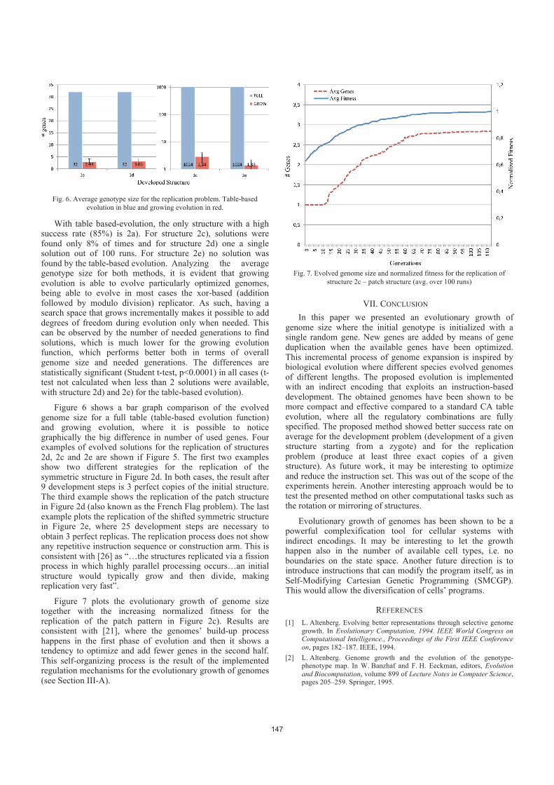
Fig. 6. Average genotype size for the replication problem. Table-based
evolution in blue and growing evolution in red.
With table based-evolution, the only structure with a high success rate (85%) is 2a). For structure 2c), solutions were found only 8% of times and for structure 2d) one a single solution out of 100 runs. For structure 2e) no solution was found by the table-based evolution. Analyzing the average genotype size for both methods, it is evident that growing evolution is able to evolve particularly optimized genomes, being able to evolve in most cases the xor-based (addition followed by modulo division) replicator. As such, having a search space that grows incrementally makes it possible to add degrees of freedom during evolution only when needed. This can be observed by the number of needed generations to find solutions, which is much lower for the growing evolution function, which performs better both in terms of overall genome size and needed generations. The differences are statistically significant (Student t-test, p<0.0001) in all cases (t-test not calculated when less than 2 solutions were available, with structure 2d) and 2e) for the table-based evolution).
Figure 6 shows a bar graph comparison of the evolved genome size for a full table (table-based evolution function) and growing evolution, where it is possible to notice graphically the big difference in number of used genes. Four examples of evolved solutions for the replication of structures 2d, 2c and 2e are shown if Figure 5. The first two examples show two different strategies for the replication of the symmetric structure in Figure 2d. In both cases, the result after 9 development steps is 3 perfect copies of the initial structure. The third example shows the replication of the patch structure in Figure 2d (also known as the French Flag problem). The last example plots the replication of the shifted symmetric structure in Figure 2e, where 25 development steps are necessary to obtain 3 perfect replicas. The replication process does not show any repetitive instruction sequence or construction arm. This is consistent with [26] as “…the structures replicated via a fission process in which highly parallel processing occurs…an initial structure would typically grow and then divide, making replication very fast”.
Figure 7 plots the evolutionary growth of genome size together with the increasing normalized fitness for the replication of the patch pattern in Figure 2c). Results are consistent with [21], where the genomes’ build-up process happens in the first phase of evolution and then it shows a tendency to optimize and add fewer genes in the second half. This self-organizing process is the result of the implemented regulation mechanisms for the evolutionary growth of genomes (see Section III-A).
Fig. 7. Evolved genome size and normalized fitness for the replication of
structure 2c – patch structure (avg. over 100 runs)
VII. CONCLUSION
In this paper we presented an evolutionary growth of genome size where the initial genotype is initialized with a single random gene. New genes are added by means of gene duplication when the available genes have been optimized. This incremental process of genome expansion is inspired by biological evolution where different species evolved genomes of different lengths. The proposed evolution is implemented with an indirect encoding that exploits an instruction-based development. The obtained genomes have been shown to be more compact and effective compared to a standard CA table evolution, where all the regulatory combinations are fully specified. The proposed method showed better success rate on average for the development problem (development of a given structure starting from a zygote) and for the replication problem (produce at least three exact copies of a given structure). As future work, it may be interesting to optimize and reduce the instruction set. This was out of the scope of the experiments herein. Another interesting approach would be to test the presented method on other computational tasks such as the rotation or mirroring of structures.
Evolutionary growth of genomes has been shown to be a powerful complexification tool for cellular systems with indirect encodings. It may be interesting to let the growth happen also in the number of available cell types, i.e. no boundaries on the state space. Another future direction is to introduce instructions that can modify the program itself, as in Self-Modifying Cartesian Genetic Programming (SMCGP). This would allow the diversification of cells’ programs.
REFERENCES
[1] L. Altenberg. Evolving better representations through selective genome
growth. In Evolutionary Computation, 1994. IEEE World Congress on Computational Intelligence., Proceedings of the First IEEE Conference
on, pages 182–187. IEEE, 1994.
[2] L. Altenberg. Genome growth and the evolution of the genotype-phenotype map. In W. Banzhaf and F. H. Eeckman, editors, Evolution
and Biocomputation, volume 899 of Lecture Notes in Computer Science, pages 205–259. Springer, 1995.
147
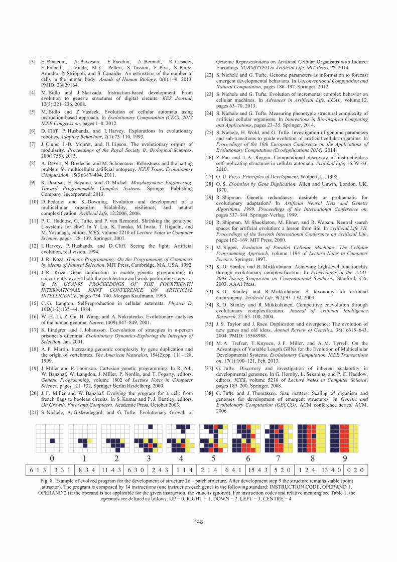
6 1 3 3 3 1 8 3 4 11 4 3 6 3 0 2 4 3 1 1 4 2 1 4 6 4 1 15 4 3 5 2 0 1 2 4 13 4 0 0 2 0
Fig. 8. Example of evolved program for the development of structure 2c – patch structure. After development step 9 the structure remains stable (point
attractor). The program is composed by 14 instructions (one instruction each gene) in the following standard: INSTRUCTION CODE, OPERAND 1,
OPERAND 2 (if the operand is not applicable for the given instruction, the value is ignored). For instruction codes and relative meaning see Table 1, the
operands are defined as follows: UP = 0, RIGHT = 1, DOWN = 2, LEFT = 3, CENTRE = 4.
[3] E. Bianconi, A. Piovesan, F. Facchin, A. Beraudi, R. Casadei,
F. Frabetti, L. Vitale, M. C. Pelleri, S. Tassani, F. Piva, S. Perez-Amodio, P. Strippoli, and S. Canaider. An estimation of the number of
cells in the human body. Annals of Human Biology, 0(0):1–9, 2013. PMID: 23829164.
[4] M. Bidlo and J. Skarvada. Instruction-based development: From evolution to generic structures of digital circuits. KES Journal,
12(3):221–236, 2008.
[5] M. Bidlo and Z. Vasicek. Evolution of cellular automata using instruction-based approach. In Evolutionary Computation (CEC), 2012
IEEE Congress on, pages 1–8, 2012.
[6] D. Cliff, P. Husbands, and I. Harvey. Explorations in evolutionary robotics. Adaptive Behaviour, 2(1):73–110, 1993.
[7] J. Clune, J.-B. Mouret, and H. Lipson. The evolutionary origins of
modularity. Proceedings of the Royal Society B: Biological Sciences, 280(1755), 2013.
[8] A. Devert, N. Bredeche, and M. Schoenauer. Robustness and the halting
problem for multicellular artificial ontogeny. IEEE Trans. Evolutionary Computation, 15(3):387–404, 2011.
[9] R. Doursat, H. Sayama, and O. Michel. Morphogenetic Engineering:
Toward Programmable Complex Systems. Springer Publishing Company, Incorporated, 2013.
[10] D. Federici and K. Downing. Evolution and development of a multicellular organism: Scalability, resilience, and neutral
complexification. Artificial Life, 12:2006, 2006.
[11] P. C. Haddow, G. Tufte, and P. van Remortel. Shrinking the genotype: L-systems for ehw? In Y. Liu, K. Tanaka, M. Iwata, T. Higuchi, and
M. Yasunaga, editors, ICES, volume 2210 of Lecture Notes in Computer Science, pages 128–139. Springer, 2001.
[12] I. Harvey, P. Husbands, and D. Cliff. Seeing the light: Artificial
evolution, real vision, 1994.
[13] J. R. Koza. Genetic Programming: On the Programming of Computers by Means of Natural Selection. MIT Press, Cambridge, MA, USA, 1992.
[14] J. R. Koza. Gene duplication to enable genetic programming to
concurrently evolve both the architecture and work-performing steps . . . In IN IJCAI-95 PROCEEDINGS OF THE FOURTEENTH
INTERNATIONAL JOINT CONFERENCE ON ARTIFICIAL INTELLIGENCE, pages 734–740. Morgan Kaufmann, 1995.
[15] C. G. Langton. Self-reproduction in cellular automata. Physica D,
10D(1-2):135–44, 1984.
[16] W.-H. Li, Z. Gu, H. Wang, and A. Nukrutenko. Evolutionary analyses
of the human genome. Nature, (409):847–849, 2001.
[17] K. Lindgren and J. Johansson. Coevolution of strategies in n-person prisoner’s dilemma. Evolutionary Dynamics-Exploring the Interplay of
Selection, Jan. 2001.
[18] A. P. Martin. Increasing genomic complexity by gene duplication and the origin of vertebrates. The American Naturalist, 154(2):pp. 111–128,
1999.
[19] J. Miller and P. Thomson. Cartesian genetic programming. In R. Poli, W. Banzhaf, W. Langdon, J. Miller, P. Nordin, and T. Fogarty, editors,
Genetic Programming, volume 1802 of Lecture Notes in Computer Science, pages 121–132. Springer Berlin Heidelberg, 2000.
[20] J. F. Miller and W. Banzhaf. Evolving the program for a cell: from
french flags to boolean circuits. In S. Kumar and P. J. Bentley, editors, On Growth, Form and Computers. Academic Press, October 2003.
[21] S. Nichele, A. Giskeødegård, and G. Tufte. Evolutionary Growth of
Genome Representations on Artificial Cellular Organisms with Indirect
Encodings. SUBMITTED to Artificial Life, MIT Press, ??, 2014.
[22] S. Nichele and G. Tufte. Genome parameters as information to forecast
emergent developmental behaviors. In Unconventional Computation and Natural Computation, pages 186–197. Springer, 2012.
[23] S. Nichele and G. Tufte. Evolution of incremental complex behavior on
cellular machines. In Advances in Artificial Life, ECAL, volume 12, pages 63–70, 2013.
[24] S. Nichele and G. Tufte. Measuring phenotypic structural complexity of
artificial cellular organisms. In Innovations in Bio-inspired Computing and Applications, pages 23–35. Springer, 2014.
[25] S. Nichele, H. Wold, and G. Tufte. Investigation of genome parameters
and sub-transitions to guide evolution of artificial cellular organims. In Proceedings of the 16th European Conference on the Applications of
Evolutionary Computation (EvoApplications 2014), 2014.
[26] Z. Pan and J. A. Reggia. Computational discovery of instructionless self-replicating structures in cellular automata. Artificial Life, 16:39–63,
2010.
[27] O. U. Press. Principles of Development. Wolpert, L., 1998.
[28] O. S. Evolution by Gene Duplication. Allen and Unwin, London, UK,
1970.
[29] R. Shipman. Genetic redundancy: desirable or problematic for evolutionary adaptation? In Artificial Neural Nets and Genetic
Algorithms, 1999. Proceedings of the International Conference on, pages 337–344. Springer-Verlag, 1999.
[30] R. Shipman, M. Shackleton, M. Ebner, and R. Watson. Neutral search
spaces for artificial evolution: a lesson from life. In Artificial Life VII, Proceedings of the Seventh International Conference on Artificial Life,
pages 162–169. MIT Press, 2000.
[31] M. Sipper. Evolution of Parallel Cellular Machines, The Cellular Programming Approach, volume 1194 of Lecture Notes in Computer
Science. Springer, 1997.
[32] K. O. Stanley and R. Miikkulainen. Achieving high-level functionality through evolutionary complexification. In Proceedings of the AAAI-
2003 Spring Symposium on Computational Synthesis, Stanford, CA, 2003. AAAI Press.
[33] K. O. Stanley and R. Miikkulainen. A taxonomy for artificial
embryogeny. Artificial Life, 9(2):93–130, 2003.
[34] K. O. Stanley and R. Miikkulainen. Competitive coevolution through
evolutionary complexification. Journal of Artificial Intelligence Research, 21:63–100, 2004.
[35] J. S. Taylor and J. Raes. Duplication and divergence: The evolution of
new genes and old ideas. Annual Review of Genetics, 38(1):615–643, 2004. PMID: 15568988.
[36] M. A. Trefzer, T. Kuyucu, J. F. Miller, and A. M. Tyrrell. On the
Advantages of Variable Length GRNs for the Evolution of Multicellular Developmental Systems. Evolutionary Computation, IEEE Transactions
on, 17(1):100–121, Feb. 2013.
[37] G. Tufte. Discovery and investigation of inherent scalability in developmental genomes. In G. Hornby, L. Sekanina, and P. C. Haddow,
editors, ICES, volume 5216 of Lecture Notes in Computer Science, pages 189–200. Springer, 2008.
[38] G. Tufte and J. Thomassen. Size matters: Scaling of organism and
genomes for development of emergent structures. In Genetic and Evolutionary Computation (GECCO), ACM conference series. ACM,
2006.
148