A NORMATIVE APPROACH TO DESIGNING FOR EVOLVABILITY:

METHODS AND METRICS FOR CONSIDERING EVOLVABILITY IN

SYSTEMS ENGINEERING

by

Daniel O’Brien Fulcoly

B.S. Physics and Mathematics United States Air Force Academy, 2010

Submitted to the Department of Aeronautics and Astronautics in Partial Fulfillment of the Requirements for the Degree of

Master of Science in Aeronautics and Astronautics

at the

Massachusetts Institute of Technology

June 2012

All rights reserved

Signature of Author……………………………………………………………………………………………………...

Department of Aeronautics and Astronautics May 23, 2012

Certified by……………………………………………………………………………………………………………...

Donna H. Rhodes Principal Research Scientist and Senior Lecturer, Engineering Systems

Director, Systems Engineering Advancement Research Initiative Thesis Supervisor

Accepted by…………………………………...…………………………………………………………………………

Adam M. Ross Research Scientist, Engineering Systems

Lead Research Scientist, Systems Engineering Advancement Research Initiative Thesis Co-Advisor

Accepted by…………………………………...…………………………………………………………………………

Daniel E. Hastings Professor of Aeronautics and Astronautics and Engineering Systems

Thesis Reader

Accepted by…………………………………...………………………………………………………………………… Eytan Modiano

Professor of Aeronautics and Astronautics Chair, Committee on Graduate Students

2

The views expressed in this article are those of the author and do not reflect the official policy or position of the United States Air Force, Department of Defense, or the U.S. Government.

3

A NORMATIVE APPROACH TO DESIGNING FOR EVOLVABILITY:

METHODS AND METRICS FOR CONSIDERING EVOLVABILITY IN

SYSTEMS ENGINEERING

by

Daniel O. Fulcoly

Submitted to the Department of Aeronautics and Astronautics on May 24, 2012 in Partial Fulfillment of the Requirements for the Degree of Master of Science in Aeronautics and Astronautics

Abstract As engineering endeavors become larger, more complex, and more expensive, the advantages of evolvable design and redesign grow. Cost and complexity are not the only factors driving the need for evolvability; changes in requirements and context can also lead to the need for redesign. This research looks to characterize evolvability, propose design principles for evolvability, determine the conditions that make designing for evolvability appropriate, and in the case of preplanned generations, determine an appropriate generation length. Evolvability is defined in this research as “the ability of an architecture to be inherited and changed across generations [over time].” This definition is used as a basis for determining a metric for measuring evolvability. The Filtered Outdegree for Evolvability metric was determined to be the most appropriate metric for measuring evolvability. The Epoch Syncopation Framework (ESF) was developed as a way of analyzing point designs, change mechanisms, execution timing, and change strategies. The ESF provides the capability to determine the conditions that make evolvability an appropriate design consideration, as well as use the temporal nature of system changes to decide on an appropriate generation length if preplanned generations are to be utilized. The Expedited Tradespace Approximation Method (ETAM) was developed in response to the heavy reliance of filtered outdegree metric and ESF on tradespace networks. ETAM leverages intelligent subsampling and interpolation methods to generate acceptable data for a large tradespace, using less computational resources than applying a performance model to every design point would normally take. All three methods were applied to case studies to demonstrate their effectiveness. A list of evolvability design principles is proposed informed by literature and findings from case study applications. The contributions of this research will enable future considerations of evolvability in systems engineering. Thesis Supervisor: Donna H. Rhodes Title: Principal Research Scientist and Senior Lecturer, Engineering Systems Co-Advisor and Thesis Reader: Adam M. Ross Title: Research Scientist, Engineering Systems

4

5

Acknowledgements The support I received while pursuing this degree and writing this thesis was invaluable; I could not have done this alone. The first people I need to thank are my family. You all have been an amazing support group throughout the last 24 years (I guess only 19 of them for you, Matt). Dad, you made me who I am today. If it wasn’t for our time testing different woods in the garage as part of the second grade science fair, I don’t think I would be as interested in science as I am today. You were a great soccer coach and introduced me to the world of rugby which has become a huge part of my life (we even got to play together again while I was in Boston!). Mom, you always been there for me. I can remember many a school project where your help and ideas helped direct my sometimes scatterbrained thoughts into work I could be proud of! You have never failed to be an insightful resource when I have questions about literally everything or just want to vent. Matt, our brotherly bond has definitely kept me sane during some of the times here that make me want to go crazy. I’m proud of everything you have done (even if watching our golf score differential grow makes me pretty jealous).

I’d like to thank all my academic mentors and teachers. Whether I was at Matthews, Schimelpfenig, Jasper, Plano Sr., USAFA, or MIT I always had the best to set me up for success. I especially want to thank Dr. Francis Chun at USAFA for showing me the ropes of research and helping me get to MIT. Thank you to SEAri not only for funding my research, but refining my skills as a researcher in a field I initially felt clueless in! To Dr. Donna Rhodes, you were a great help in showing me how to communicate my research both by the example you set and the mentoring you gave. To Dr. Adam Ross, thank you so much for the countless hours you put into helping me along this path. You were always patient and understanding while simultaneously making sure that I was doing research I could be proud of. Our weekly meetings were never boring, and the tangents we went off on sometimes spawned great new research threads (or occasionally just much-needed physicist talk!). Other fellow students were crucial to my success here as well. Matt Fitzgerald, thanks for being helpful when I was slow to pick up on some of the changeability code. Our games of Space Tug Skirmish (to ska background music, of course) were never dull. Nirav Shah, thank you for all the help you provided. You were the resident expert on everything from pottery to biology, and you used your wealth of knowledge to help me do better research (especially on ETAM!).

Finally, I’d like to thank the friends I had here in Boston. Clark and Ben, the times we shared as roommates were amazing. From weeknight activities at Thorndike to Parish excursions to fabulous nights in Boston, we definitely created some great stories together. To the Boston Irish Wolfhounds, thank you for the great rugby experience. You made me feel right at home ever since my first practice, and it was an honor to wear the green and white with you guys all over the country! Last but not least, thank you to the great group of friends known only as the “Broman Empire.” You guys were amazing and made sure there was never a dull weekend. Without the great weekends we shared, my sanity would sure not be intact.

6

7

Biographical Note Daniel Fulcoly holds Bachelor of Science degrees in Mathematics and Physics from the United States Air Force Academy, where he was a distinguished graduate of the Class of 2010. He will graduate from the Massachusetts Institute of Technology in June of 2012 with a Master of Science in Aeronautics and Astronautics. During his time at MIT, he was a research assistant in the Systems Engineering Advancement Research Initiative (SEAri).

Dan was born and raised in Plano, TX, a large suburb north of Dallas. His love for science began in elementary school when he participated in many science fairs and discovered how much there was to learn and how exciting it could be. Another outlet he enjoyed was sports; Dan was an avid soccer, football, and rugby player. Dan was first introduced to service through participation in the Boy Scouts of America. His appreciation for service, along with a never dying desire to become an astronaut, led to Dan joining the United States Air Force Academy (USAFA) in the summer of 2006.

At USAFA, Dan strove to excel in all facets of cadet life. He played for the USAFA rugby team all four years, a team that twice advanced to the sweet 16 at the highest level of college rugby in the USA. He served in many military positions, culminating in commanding a squadron of over 140 cadets and basic cadets during basic cadet training. In the academic realm, Dan pursued two technical majors while broadening his non-technical education through the Academy Scholars Program.

Research was a significant aspect of Dan’s time at USAFA. He began researching in the fields of Space Situational Awareness (SSA) and Non-Resolvable Space Object Identification in the spring of 2009. Over the next year and a half, he presented his research at two conferences, two workshops, and eventually published his work in a peer-reviewed journal. His research not only earned him many distinctions and awards at USAFA, but played a critical role in setting him up for success as a researcher at MIT.

After graduation from MIT, Dan will serve as a physicist in the United States Air Force at Kirtland Air Force Base in New Mexico, where he hopes to return to the field of SSA. Ultimately he would like to become a flight test engineer for the USAF and continue pursuing his dream of being an astronaut.

8

9

Table of Contents

ABSTRACT ................................................................................................................................... 3 

ACKNOWLEDGEMENTS ......................................................................................................... 5 

BIOGRAPHICAL NOTE ............................................................................................................ 7 

TABLE OF CONTENTS ............................................................................................................. 9 

LIST OF FIGURES .................................................................................................................... 13 

LIST OF TABLES ...................................................................................................................... 15 

1  INTRODUCTION............................................................................................................... 17 

1.1  MOTIVATION .................................................................................................................. 17 1.2  RESEARCH SCOPE & METHODOLOGY ............................................................................ 17 

1.2.1  Research Approach and Questions ........................................................................... 17 1.2.2  Related Concepts and Methods ................................................................................. 19 

1.3  OVERVIEW OF THESIS .................................................................................................... 22 

2  DEFINING AND CONSIDERING EVOLVABILITY IN SYSTEMS .......................... 25 

2.1  DEFINING EVOLVABILITY .............................................................................................. 25 2.1.1  Existing Definitions ................................................................................................... 25 2.1.2  Synthesis .................................................................................................................... 28 

2.2  EXISTING DESIGN CONSIDERATIONS .............................................................................. 28 2.2.1  Under What Conditions Should Evolvability be a Design Consideration? .............. 29 2.2.2  What Design Principles Have Been Proposed?........................................................ 29 

2.3  SUMMARY ...................................................................................................................... 30 

3  DEVELOPING AND APPLYING METRICS FOR EVOLVABILITY ....................... 33 

3.1  EVALUATING EXISTING METRICS .................................................................................. 33 3.1.1  Metric Criteria .......................................................................................................... 33 3.1.2  Candidate Metrics ..................................................................................................... 35 

3.1.2.1  Interface Complexity Metric (Holtta-Otto 2005) .............................................. 35 3.1.2.2  Ontological Approach (Rowe and Leaney 1997) ............................................. 36 3.1.2.3  Visibility Matrix (MacCormack et al. 2007) .................................................... 37 3.1.2.4  Filtered Outdegree (Ross et al. 2008b) ............................................................. 39 

3.1.3  Selecting the Metric: Filtered Outdegree for Evolvability ....................................... 40 3.2  APPLICATION TO SPACE TUG ......................................................................................... 40 

3.2.1  Tradespace Definition ............................................................................................... 41 3.2.2  Change Mechanism ................................................................................................... 42 3.2.3  Results: Calculation of Filtered Outdegree .............................................................. 44 

10

3.3  CONCLUSIONS ................................................................................................................ 50 

4  EPOCH SYNCOPATION FRAMEWORK ..................................................................... 51 

4.1  OVERVIEW ..................................................................................................................... 51 4.1.1  Motivation ................................................................................................................. 51 4.1.2  Prior Methods ........................................................................................................... 51 

4.1.2.1  Technology Syncopation Framework (Beesemyer et al. 2011) ........................ 52 4.1.2.2  Time-Expanded Decision Networks (Silver and de Weck 2007) ..................... 54 4.1.2.3  Decision Tree Analysis and Binomial Lattice Models (Cardin 2011) .............. 55 4.1.2.4  ESF Intended Contributions .............................................................................. 57 

4.1.3  ESF Architecture ....................................................................................................... 58 4.2  ESF PROCESS ................................................................................................................. 58 

4.2.1  Inputs......................................................................................................................... 59 4.2.1.1  Epoch Variables and Change Parameters ......................................................... 59 4.2.1.2  Design Transition Matrices ............................................................................... 59 4.2.1.3  Design Set and Initial Design ........................................................................... 59 4.2.1.4  Change Strategies .............................................................................................. 59 

4.2.2  Era Constructor ........................................................................................................ 60 4.2.3  Era Simulation and Outputs...................................................................................... 61 

4.3  APPLICATION TO SPACE TUG ......................................................................................... 62 4.3.1  Epoch Variables ........................................................................................................ 62 4.3.2  Tradespace Definition ............................................................................................... 66 4.3.3  Change Mechanism ................................................................................................... 68 4.3.4  Results: Application of ESF ...................................................................................... 69 

4.3.4.1  Experimental Setup ........................................................................................... 69 4.3.4.2  Outputs .............................................................................................................. 70 

4.3.5  Discussion ................................................................................................................. 72 4.4  ESF LITE ....................................................................................................................... 75 

5  EXPEDITED TRADESPACE APPROXIMATION METHOD (ETAM) .................... 77 

5.1  OVERVIEW ..................................................................................................................... 77 5.1.1  Motivation ................................................................................................................. 77 5.1.2  Overview of ETAM .................................................................................................... 79 5.1.3  Existing Methods ....................................................................................................... 79 

5.2  IMPLEMENTATION .......................................................................................................... 81 5.2.1  Partitioning the enumerated tradespace ................................................................... 82 5.2.2  Selecting the training set (using DOE) ..................................................................... 84 5.2.3  Setting up Kriging and interpolating “missing” points ............................................ 89 5.2.4  How ordinary Kriging works (Chiles & Delfiner 1999) ........................................... 89 5.2.5  Computational implementation (Press et al. 2007) .................................................. 91 

5.3  APPLICATION TO SATELLITE RADAR .............................................................................. 93 

11

5.3.1  Variable Handling .................................................................................................... 93 5.3.2  Results ....................................................................................................................... 93 

5.4  APPLICATION TO SPACE TUG ....................................................................................... 100 5.4.1  Variable Handling .................................................................................................. 100 5.4.2  Results ..................................................................................................................... 103 

5.5  DISCUSSION ................................................................................................................. 109 5.6  CONSIDERATIONS FOR APPLYING ETAM .................................................................... 109 

5.6.1  Limitations .............................................................................................................. 109 5.6.2  Potential Savings .................................................................................................... 110 5.6.3  Potential Costs ........................................................................................................ 111 

6  DISCUSSION .................................................................................................................... 113 

6.1  REVISITING RESEARCH QUESTIONS ............................................................................. 113 6.1.1  Design Principles .................................................................................................... 113 

6.1.1.1  Design Principles from Metrics ...................................................................... 115 6.1.1.2  Design Principles from the ESF ...................................................................... 115 6.1.1.3  Design principles from the proposed evolvability definition ......................... 116 

6.1.2  Enabling Exploration of Large Tradespaces Using ETAM .................................... 116 6.2  LIMITATIONS AND CHALLENGES .................................................................................. 116 

7  CONCLUSIONS ............................................................................................................... 117 

7.1  CONTRIBUTIONS .......................................................................................................... 117 7.2  FUTURE WORK ............................................................................................................ 119 

8  REFERENCES .................................................................................................................. 121 

12

13

List of Figures Figure 1-1. Dual approach to developing evolvability design principles .................................... 18 Figure 1-2. Architecture - Design - System Hierarchy ................................................................. 20 Figure 1-3. Data Flow .................................................................................................................. 22 Figure 1-4. The Anatomy of a Change Option with Path Enabler and Change Mechanism (M1)(Ross and Rhodes 2011)........................................................................................................ 22 Figure 2-1. The Evolution of an Architecture over Time.............................................................. 28 Figure 3-1. Interface Complexity Metric (adapted from Holtta-Otto 2005) ................................ 35 Figure 3-2. Example System Diagram and M1 Matrix (MacCormack et al. 2007) ...................... 37 Figure 3-3. Derivation of Visibility Matrix (adapted from MacCormack et al. 2007) ................. 38 Figure 3-4. Using Transition Rules to Transform a Tradespace into a Tradespace Network (Ross et al. 2008b) .................................................................................................................................. 39 Figure 3-5. Depiction of Redesign Schedule ................................................................................ 43 Figure 3-6. Filtered Outdegree for Evolvability Applied to Space Tug ....................................... 45 Figure 3-7. Filtered Outdegree of a Design for Different Propulsion systems (Transition Cost on x-axis) ............................................................................................................................................ 46 Figure 3-8. Filtered Outdegree of a Design for Different Manipulator Masses .......................... 47 Figure 3-9. DfE Adjusted Filtered Outdegree Comparison for Design 1 (300kg Manipulator, 30kg Fuel, Storable Bipropellant) ................................................................................................ 48 Figure 3-10. DfE Adjusted Filtered Outdegree Comparison for Design 100 (5,000kg Manipulator, 600kg Fuel, Storable Bipropellant) ........................................................................ 48 Figure 3-11. Mean Filtered Outdegree by Design Variable Levels ............................................. 49 Figure 4-1. Net Context Frequency Derived from Epoch Variable Component Frequencies ..... 52 Figure 4-2. Sample TSF Simulation with a 5 Year Generation Length ........................................ 53 Figure 4-3. Costs Corresponding to the TSF Simulation seen in Figure 4-2 ............................... 54 Figure 4-4. Visualization of the TDN (Silver and de Weck 2007) ................................................ 55 Figure 4-5. Example Decision Tree Analysis (Cardin 2011) ....................................................... 56 Figure 4-6. Example Binomial Lattice Model .............................................................................. 57 Figure 4-7. Architecture of the ESF ............................................................................................. 58 Figure 4-8. Mechanics of the Markov Probability Era Constructor ............................................ 61 Figure 4-9. Single Attribute Utility Curves for Manipulator Mass .............................................. 64 Figure 4-10. Single Attribute Utility Curves for Response Time .................................................. 64 Figure 4-11. Single Attribute Utility Curves for Delta V .............................................................. 65 Figure 4-12. Cost-Utility-Schedule Tradespace for All Designs Valid in Mission 8. .................. 68 Figure 4-13. Convergence of ESF Outputs ................................................................................... 70 Figure 4-14. Average Lifecycle Cost vs. Generation Length for Space Tug ................................ 74 Figure 4-15. Average TWAU vs. Generation Length for Space Tug ............................................ 74 Figure 5-1. Tradespace Growth Assuming All Combinations Allowed ........................................ 78 Figure 5-2. Overview of the ETAM ............................................................................................... 79 Figure 5-3. General VisualDOC Structure (Balabanov et al. 2002) ............................................ 81 

14

Figure 5-4. Dependency diagram between Minimum RCS and Krigable Variables for Epoch 1 86 Figure 5-5. Dependency diagram between Number of Boxes and Krigable Variables for Epoch 1....................................................................................................................................................... 86 Figure 5-6. Set relationships for Satellite Radar .......................................................................... 89 Figure 5-7. Correlations of the attributes dependent on >2 Krigable variables ......................... 94 Figure 5-8. Error distributions of the attributes dependent on >2 Krigable variables ............... 95 Figure 5-9. Correlation between Kriged SAU and Actual SAU for Kriged attributes ................. 96 Figure 5-10. Kriged values vs. actual values for number of boxes, zoomed to [0, 1] SAU range from Figure 5-7 ............................................................................................................................. 97 Figure 5-11. SAU curve (normal and log scale) for targets per pass .......................................... 98 Figure 5-12. Correlation between Kriged MAU and Actual MAU for Satellite Radar ................ 99 Figure 5-13. Cost and Delta V Correlations and Error Distributions for 32 Training Points .. 104 Figure 5-14. Spearman Rho Values vs. Training Set Size (as a percent of Krigable subset, N = 96) ............................................................................................................................................... 105 Figure 5-15. Correlation of Kriged vs. Actual Delta V Values for Different Training Set Sizes (Clockwise from top left: 17, 25, 40, 51) .................................................................................... 106 Figure 5-16. Distribution of Errors in Delta V for Different Training Set Sizes (Clockwise from top left: 17, 25, 40, 51) ................................................................................................................ 107 Figure 5-17. Mean and Standard Deviation of Difference between Actual and Kriged Attributes for Space Tug .............................................................................................................................. 108 Figure 5-18. Percent Error in Attributes vs. Size of Training Set .............................................. 109 Figure 5-19. Training set implications stemming from including the points on the surface of an n-dimensional hyper cube (n = 2 shown). This does not consider additional points that would be in the training set as selected by DOE. ....................................................................................... 110 Figure 7-1. Transition Rules Help Form Tradespace Networks Suitable for Applying Filtered Outdegree to................................................................................................................................ 118 Figure 7-2. The Epoch Syncopation Framework ........................................................................ 118 Figure 7-3. The Expedited Tradespace Approximation Method ................................................ 119 

15

List of Tables Table 2-1. Existing Design Principles for Evolvability ................................................................ 31 Table 3-1. Metric Scores for Interface Complexity Metric ........................................................... 36 Table 3-2. Metric Scores for Ontological Approach .................................................................... 37 Table 3-3. Metric Scores for Visibility Matrix .............................................................................. 39 Table 3-4. Metric Scores for Filtered Outdegree ......................................................................... 40 Table 3-5. Overview of Metric Scores .......................................................................................... 40 Table 3-6. Design Variable Levels (modified from McManus and Schuman 2003) ..................... 41 Table 3-7. Propulsion System Values (McManus and Schuman 2003) ........................................ 41 Table 4-1. Inputs for Change Strategies ....................................................................................... 60 Table 4-2. Hypothetical Markov Transition Matrix for Preference Sets (Space Tug "Missions") 63 Table 4-3. SAU Curves and Weights for Space Tug Missions ...................................................... 63 Table 4-4. Markov Transition Matrix for Technology Level ........................................................ 66 Table 4-5. Design Variable Levels (modified from McManus and Schuman 2003) ..................... 66 Table 4-6. Propulsion System Values (McManus and Schuman 2003) ........................................ 66 Table 4-7. Inputs for Change Strategies ....................................................................................... 69 Table 4-8. Inputs for Change Strategies ....................................................................................... 71 Table 4-9. Description of Trials.................................................................................................... 71 Table 4-10. Results of 11 ESF Trials ............................................................................................ 72 Table 4-11. Designs of Interest ..................................................................................................... 73 Table 4-12. Example Application of ESF Lite .............................................................................. 75 Table 5-1. Variable Types (Siegel 1957) ...................................................................................... 82 Table 5-2. Design Variable List for Satellite Radar (Krigable variables are italicized) ............. 83 Table 5-3. Epoch Variable List for Satellite Radar (Krigable variables are italicized) .............. 83 Table 5-4. Box-Benkhen Savings for Three-Level Variables ........................................................ 85 Table 5-5. Binary DMM for Satellite Radar (‘X’ indicated dependence) .................................... 87 Table 5-6. Training Sets for Satellite Radar ................................................................................. 88 Table 5-7. Accuracy of Kriged Variables ..................................................................................... 93 Table 5-8. Spearman's Rank Correlation Coefficients for SAU and MAU Values ..................... 100 Table 5-9. Design Variable Levels (McManus and Schuman 2003, Fulcoly et al. 2012) Krigable Variables are Italicized ............................................................................................................... 101 Table 5-10. Propulsion System Values (McManus and Schuman 2003) .................................... 101 Table 5-11. Binary DMM for Space Tug .................................................................................... 103 Table 5-12. Accuracy of Kriged Variables (32 Training Points) Over 50 Full Executions of ETAM .......................................................................................................................................... 104 Table 5-13. Time Dilation Factor for Different Case Studies .................................................... 111 Table 6-1. Existing Design Principles for Evolvability .............................................................. 114 Table 7-1. Candidate Design Principles for Evolvability ........................................................... 117 

16

17

1 Introduction The early phases of conceptual design require careful consideration as early decisions will have substantial influence on the new system, ultimately enabling or limiting success of the system over time. Looking beyond traditional performance metrics, measuring a system’s “ilities” such as changeability, adaptability, flexibility, and survivability gives stakeholders and decision makers an enhanced basis for differentiating between design alternatives. These different ilities consider aspects of a system that might not be captured by measuring performance in a static environment, such as how its value can change due to changing form (changeability) or how well the system reacts to disturbances in its environment (survivability). Evolvability is a design characteristic that facilitates more manageable transitions between system generations via the modification of an inherited architecture. Epochs are periods of fixed contexts and needs; in the face of changing epochs, systems can be designed to change in response, or remain robust, in order to retain useful functionality to avoid suffering deficiencies and even failure (Ross 2006). Designing an evolvable system may reduce the long term cost of system upgrades or replacements in the presence of epoch shifts over its lifespan.

1.1 Motivation

As engineering endeavors become larger, more complex, and more expensive, the advantages of evolvable design grow. Evolvable design starts from an existing design, rather than a blank slate, and is an increasingly common trend; for example nearly 85% of GE’s products are modifications of previous products (Holtta-Otto 2005). In industries where redesign is the norm, evolvability clearly is a desirable trait. Cost and complexity are not the only factors driving the need for evolvability; changes in requirements and context can also lead to the need for redesign. Suk Suh captures this concept when he explains how “system requirements change over time; consequently, companies need to systematically evolve their products to cope with those changes. Since developing a system from scratch is time consuming and costly, new systems are often created by evolving an existing system” (Suk Suh et al. 2008). As for the prevalence of changing contexts, Kevin Kelly asserts that “instability and imbalance are the norm in today’s economy, and therefore systems optimized to a single design point will not last very long” (Kelly 1998).

1.2 Research Scope & Methodology

1.2.1 Research Approach and Questions

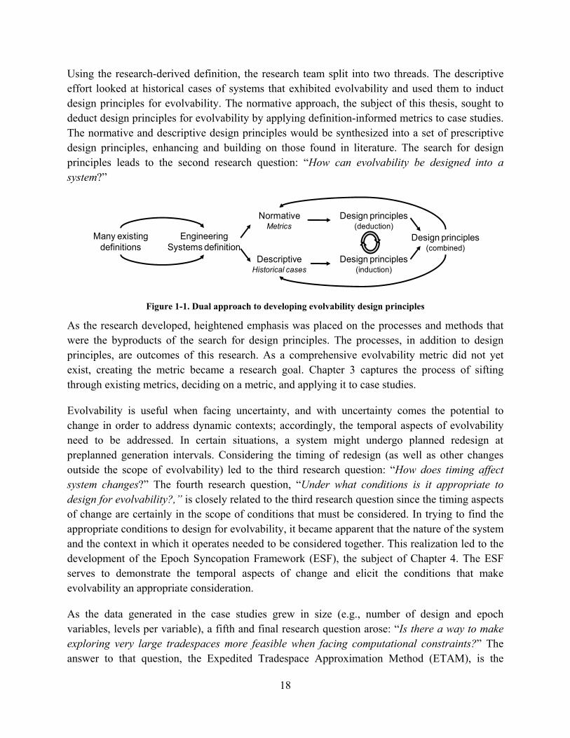
At the onset of this research, this thesis was intended to be a companion thesis to a corresponding descriptive study of evolvability culminating in a set of prescriptive design principles for evolvability. These design principles would ideally shed light on when evolvability should be a consideration and how to make a system evolvable. The beginning of this process, seen in Figure 1-1, was to develop a systems engineering definition for evolvability informed by existing definitions from literature. This represents the first research question: “What is evolvability?”

18

Using the research-derived definition, the research team split into two threads. The descriptive effort looked at historical cases of systems that exhibited evolvability and used them to induct design principles for evolvability. The normative approach, the subject of this thesis, sought to deduct design principles for evolvability by applying definition-informed metrics to case studies. The normative and descriptive design principles would be synthesized into a set of prescriptive design principles, enhancing and building on those found in literature. The search for design principles leads to the second research question: “How can evolvability be designed into a system?”

Figure 1-1. Dual approach to developing evolvability design principles

As the research developed, heightened emphasis was placed on the processes and methods that were the byproducts of the search for design principles. The processes, in addition to design principles, are outcomes of this research. As a comprehensive evolvability metric did not yet exist, creating the metric became a research goal. Chapter 3 captures the process of sifting through existing metrics, deciding on a metric, and applying it to case studies.

Evolvability is useful when facing uncertainty, and with uncertainty comes the potential to change in order to address dynamic contexts; accordingly, the temporal aspects of evolvability need to be addressed. In certain situations, a system might undergo planned redesign at preplanned generation intervals. Considering the timing of redesign (as well as other changes outside the scope of evolvability) led to the third research question: “How does timing affect system changes?” The fourth research question, “Under what conditions is it appropriate to design for evolvability?,” is closely related to the third research question since the timing aspects of change are certainly in the scope of conditions that must be considered. In trying to find the appropriate conditions to design for evolvability, it became apparent that the nature of the system and the context in which it operates needed to be considered together. This realization led to the development of the Epoch Syncopation Framework (ESF), the subject of Chapter 4. The ESF serves to demonstrate the temporal aspects of change and elicit the conditions that make evolvability an appropriate consideration.

As the data generated in the case studies grew in size (e.g., number of design and epoch variables, levels per variable), a fifth and final research question arose: “Is there a way to make exploring very large tradespaces more feasible when facing computational constraints?” The answer to that question, the Expedited Tradespace Approximation Method (ETAM), is the

Engineering Systems definition

Many existing definitions

NormativeMetrics

DescriptiveHistorical cases

Design principles (deduction)

Design principles (induction)

Design principles (combined)

19

subject of Chapter 5. While developed to support the research in this thesis, ETAM is an example of a technique that is not exclusively applicable to evolvability studies, but rather something that should help in any endeavor requiring the exploration of a very large tradespace.

So, to summarize, the research questions addressed in the research and discussed in this thesis are:

1. What is evolvability in the context of systems engineering? 2. How can evolvability be designed into a system? 3. How does timing affect system changes? 4. Under what conditions is it appropriate to design evolvability into a system? 5. Is there a way to make exploring very large tradespaces more feasible when facing computational

constraints?

1.2.2 Related Concepts and Methods

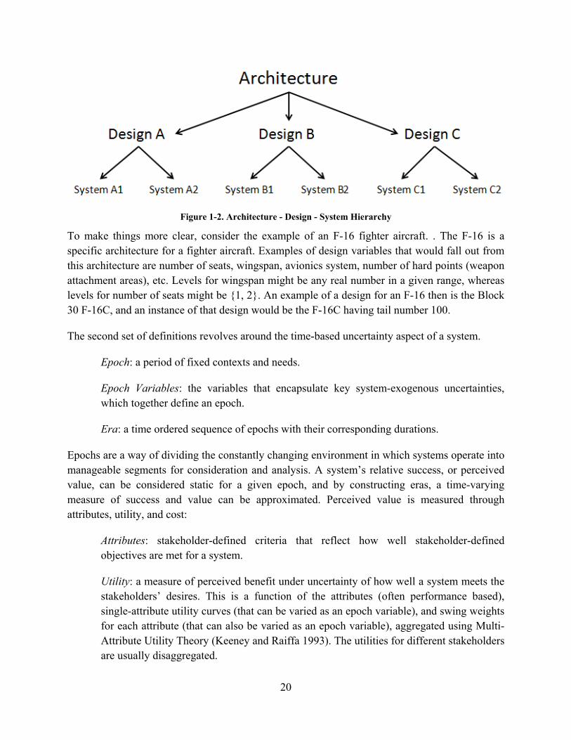
The methods used in this thesis utilize several terms that must be well understood to internalize the concepts being presented (Ross et al. 2008a). The use of these terms allows the different methods (used in chapters 3, 4, and 5) to be explained and examined on a common basis. The first set of definitions revolves around the concept of an architecture – design – system instance hierarchy as seen in Figure 1-2.

Architecture: the mapping of form to function that allows for design variables to be specified. It includes a set of allowable designs.

Design: the collection of particular choices for each design level of each design variable that collectively define a specific design.

Instance: a selected point from a given set. For example, a design is an instance of an architecture and a specific system is an instance of a design.

Design Variables: the variables, which are within the control of the designer, that are needed to specify a design. Ideally design variables drive value metrics of interest to stakeholders.

Levels: allowed values for a design variable or an epoch variable (defined below), to take.

20

Figure 1-2. Architecture - Design - System Hierarchy

To make things more clear, consider the example of an F-16 fighter aircraft. . The F-16 is a specific architecture for a fighter aircraft. Examples of design variables that would fall out from this architecture are number of seats, wingspan, avionics system, number of hard points (weapon attachment areas), etc. Levels for wingspan might be any real number in a given range, whereas levels for number of seats might be {1, 2}. An example of a design for an F-16 then is the Block 30 F-16C, and an instance of that design would be the F-16C having tail number 100.

The second set of definitions revolves around the time-based uncertainty aspect of a system.

Epoch: a period of fixed contexts and needs.

Epoch Variables: the variables that encapsulate key system-exogenous uncertainties, which together define an epoch.

Era: a time ordered sequence of epochs with their corresponding durations.

Epochs are a way of dividing the constantly changing environment in which systems operate into manageable segments for consideration and analysis. A system’s relative success, or perceived value, can be considered static for a given epoch, and by constructing eras, a time-varying measure of success and value can be approximated. Perceived value is measured through attributes, utility, and cost:

Attributes: stakeholder-defined criteria that reflect how well stakeholder-defined objectives are met for a system.

Utility: a measure of perceived benefit under uncertainty of how well a system meets the stakeholders’ desires. This is a function of the attributes (often performance based), single-attribute utility curves (that can be varied as an epoch variable), and swing weights for each attribute (that can also be varied as an epoch variable), aggregated using Multi-Attribute Utility Theory (Keeney and Raiffa 1993). The utilities for different stakeholders are usually disaggregated.

21

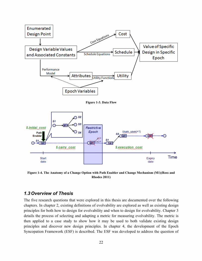
Cost: a measure of resources required to achieve a system, which is usually disaggregated as dollar costs for different stakeholders. Cost can consist of operations cost, acquisition cost, and transition costs. If not specified, cost will only refer to acquisition costs in dollars.

Value: a measure of how well a system meets stakeholder needs, typically a result of balancing benefits, costs, and uncertainty.

Since the definition of utility for a given stakeholder is fixed within an epoch, designs can be assessed on the basis of utility and cost. However, since epochs may change, a system’s design may need to be changed as well in order to deliver acceptable value to stakeholders in a new context. A system may transition to a different design to achieve a new utility via the concepts in the final set of definitions revolving around design change:

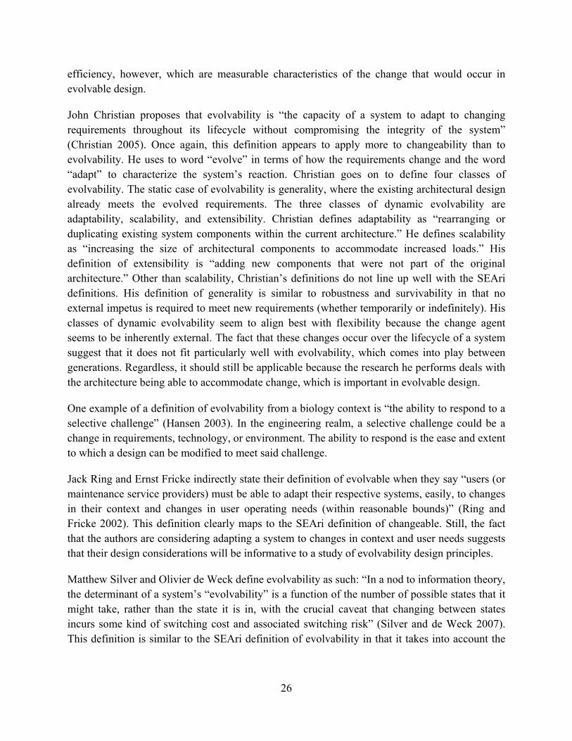
Path Enablers: features included in a design that allow a system to make certain design transitions that may not have been available otherwise (for a given resource threshold). One path enabler could enable multiple different design transitions.

Change Mechanism: the specific way that a design undergoes change to another design, with corresponding change cost and time.

Change Option: the pair of path enabler and change mechanism, which together are means by which a system can change into a different design. Inclusion of the path enabler often entails an upfront cost, but not always (if the path enabler is a latent part of an existing design), and execution of the change mechanism often entails an execution cost.

These last concepts are crucial to measuring and characterizing evolvability, as without change, there is no evolution. Many of the concepts in this section are captured in Figure 1-3, which shows how data flows when these constructs are in use. The anatomy of a change option can be seen in Figure 1-4. The epoch-era construct will be explored more in chapter 4.

22

Figure 1-3. Data Flow

Figure 1-4. The Anatomy of a Change Option with Path Enabler and Change Mechanism (M1)(Ross and Rhodes 2011)

1.3 Overview of Thesis The five research questions that were explored in this thesis are documented over the following chapters. In chapter 2, existing definitions of evolvability are explored as well as existing design principles for both how to design for evolvability and when to design for evolvability. Chapter 3 details the process of selecting and adapting a metric for measuring evolvability. The metric is then applied to a case study to show how it may be used to both validate existing design principles and discover new design principles. In chapter 4, the development of the Epoch Syncopation Framework (ESF) is described. The ESF was developed to address the question of

23

what conditions make designing for evolvability appropriate, keeping in mind the temporal aspects of change. The ESF also addresses how to choose a generation length when preplanned generations will be used. The subsequent application to a case study shows how to use the ESF to determine if evolvability is appropriate and for choosing a generation length when it is appropriate. Chapter 5 explains in detail the motivation for and development of the Expedited Tradespace Approximation Method (ETAM) that aims to use design of experiments and interpolation to generate acceptable tradespace data while saving computational resources. Chapter 6 ties the previous three chapters back to the research questions by means of discussion of results and insights. Conclusions are presented in chapter 7.

24

25

2 Defining and Considering Evolvability in Systems This thesis covers many different topics surrounding evolvability: how to define evolvability, how to design for evolvability, how to measure evolvability, how to choose strategies and make design choices based on the timing of context changes, and how to approximate data in large tradespaces. Each of these topics is related to a specific subset of literature with varying degrees of overlap. For this reason, the literature review has a central component covering defining evolvability and existing design principles as well as distributed components covering the literature related to specific methods (in chapters 3, 4, and 5).

2.1 Defining Evolvability

In engineering literature, the “ility” words are notoriously ill-defined and overlapping. Different research labs and institutions tend to use their own definitions of “ilities” based on their concepts of how they fit into engineering systems. As the number of “ilities” in use increases and as “ility” statements begin to appear in formal requirements, the need for standardized and unambiguous definitions increases1. Some researchers propose reconciling varying definitions through use of a semantic basis that would map characteristics to one or more “-ilities” (Beesemyer et al. 2012).

The definition of evolvability that was used for the purpose of this research is “the ability of an architecture to be inherited and changed across generations [over time].” More about the development of this definition can be seen in chapter 6.1. In much of the literature that was explored, adaptability and flexibility were often defined similarly to evolvability (or evolvability was defined similarly to adaptability and flexibility). The definitions for these terms that were used in the research are based on those used by researchers in the MIT Systems Engineering Advancement Research Initiative (SEAri) group: adaptability is “the ability of a system to be changed by a system-internal change agent with intent” and flexibility is “the ability of a system to be changed by a system external change agent with intent.” All three of these definitions are, in the SEAri context, subsets of changeability: “the ability of a system to alter its form – and consequently possibly its function – at an acceptable level of resource expenditure.” A review of engineering literature concerning any of these “ilities” revealed many different definitions.

2.1.1 Existing Definitions

Daniel Borches and Maarten Bonnema define evolvability as “a system’s ability to adapt to changing requirements throughout its lifespan in a time-efficient and cost-efficient way” (Borches and Bonnema 2009). This definition clearly matches more to changeability and adaptability than to evolvability. This definition focuses on a lifespan of a system and not on the redesign that would occur between generations. The definition does mention time- and cost-

1 Between April 2008 and February 2012, the crowd-sourced list of “ilities” on Wikipedia grew from 61 to 81 (Ross 2012).

26

efficiency, however, which are measurable characteristics of the change that would occur in evolvable design.

John Christian proposes that evolvability is “the capacity of a system to adapt to changing requirements throughout its lifecycle without compromising the integrity of the system” (Christian 2005). Once again, this definition appears to apply more to changeability than to evolvability. He uses to word “evolve” in terms of how the requirements change and the word “adapt” to characterize the system’s reaction. Christian goes on to define four classes of evolvability. The static case of evolvability is generality, where the existing architectural design already meets the evolved requirements. The three classes of dynamic evolvability are adaptability, scalability, and extensibility. Christian defines adaptability as “rearranging or duplicating existing system components within the current architecture.” He defines scalability as “increasing the size of architectural components to accommodate increased loads.” His definition of extensibility is “adding new components that were not part of the original architecture.” Other than scalability, Christian’s definitions do not line up well with the SEAri definitions. His definition of generality is similar to robustness and survivability in that no external impetus is required to meet new requirements (whether temporarily or indefinitely). His classes of dynamic evolvability seem to align best with flexibility because the change agent seems to be inherently external. The fact that these changes occur over the lifecycle of a system suggest that it does not fit particularly well with evolvability, which comes into play between generations. Regardless, it should still be applicable because the research he performs deals with the architecture being able to accommodate change, which is important in evolvable design.

One example of a definition of evolvability from a biology context is “the ability to respond to a selective challenge” (Hansen 2003). In the engineering realm, a selective challenge could be a change in requirements, technology, or environment. The ability to respond is the ease and extent to which a design can be modified to meet said challenge.

Jack Ring and Ernst Fricke indirectly state their definition of evolvable when they say “users (or maintenance service providers) must be able to adapt their respective systems, easily, to changes in their context and changes in user operating needs (within reasonable bounds)” (Ring and Fricke 2002). This definition clearly maps to the SEAri definition of changeable. Still, the fact that the authors are considering adapting a system to changes in context and user needs suggests that their design considerations will be informative to a study of evolvability design principles.

Matthew Silver and Olivier de Weck define evolvability as such: “In a nod to information theory, the determinant of a system’s “evolvability” is a function of the number of possible states that it might take, rather than the state it is in, with the crucial caveat that changing between states incurs some kind of switching cost and associated switching risk” (Silver and de Weck 2007). This definition is similar to the SEAri definition of evolvability in that it takes into account the

27

states reachable through inheritance, since the change paths start at the original design and do not occur in the operations phase.

David Rowe and John Leaney define evolvability as “the ability of a system to adapt to, or cope with change in its requirements, environment and implementation technologies” (Rowe and Leaney 1997). While the word adapt is used in this definition, it does not necessarily map to changeable or adaptable. They do allude to the fact that evolvability increases a system’s lifespan and decreases the maintenance costs, but the framework they introduce later in the paper does not strictly apply to in situ modifications of a system.

Rick Steiner’s definition of system evolution is the best match to the way the SEAri evolvability definition relates to changeability. He contrasts the ideas of maturation and evolution:

Taking a cue from the biological sciences, this paper draws the distinction between 1) change encountered in a single generation of a system (maturation), and 2) change encountered between subsequent generations of a family (or genus) of systems (evolution). Maturation, in this context, refers to the development of a specific system design, from initial context & concept through production & disposal. There may be many individual systems produced as part of the production run, but they are usually all from a single generation of the design. Evolution refers to how the system design changes from one generation of a product design to the next, such as specifying which elements of the design are passed down/reused, and which elements of the design are new to the latest generation. (Steiner 1998, 3).

His concept of maturation maps well to the SEAri definition of changeability.

Most of the definitions previously stated have been easily comparable to either evolvability or adaptability. However, other frameworks exist that focus less on the –ility nature of evolution. For example, rather than seeing evolution as a design evolving, Alan MacCormack et al. (2007) look at a component’s undergoing evolution as a population. The components that last throughout many design changes are “harder to kill” and therefore more evolvable. The authors further break evolution into three aspects, component survival, component maintainability, and component augmentation. Component survival is an indicator of the degree to which components can be removed or substituted over time. Component maintainability is a measure of the stability of legacy components in a design. Component augmentation is a measure of the ease with which new components can be added to a design (MacCormack et al. 2007). While this construct looks at a different issue, their results are still applicable to our evolvability framework. Judging the degree of component augmentation in particular would be useful for identify evolvable designs; being able to easily add new components would certainly make a design evolvable.

Another slightly different use of evolution in engineering systems is the concept of evolutionary acquisition. Nirav Shah cites Lawrence Delaney’s explanation of this concept: “an attempt to deliver core operational capability sooner by dividing a large, single development into many smaller developments or increments” (Shah 2004). While this idea does not directly correlate to designing for evolvability, it represents a scenario where having an evolvable system is

28

beneficial. An evolvable system lends itself to sustaining periodic modifications and improvements.

2.1.2 Synthesis

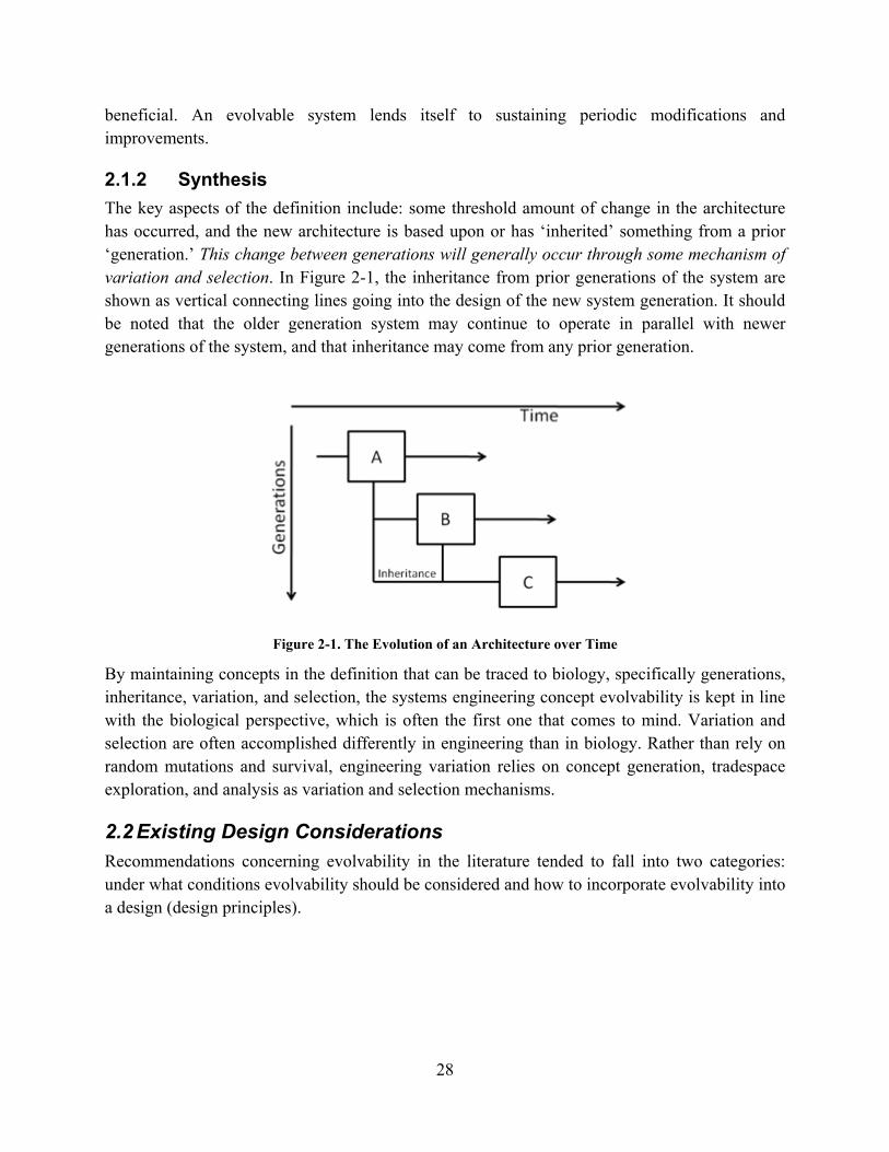
The key aspects of the definition include: some threshold amount of change in the architecture has occurred, and the new architecture is based upon or has ‘inherited’ something from a prior ‘generation.’ This change between generations will generally occur through some mechanism of variation and selection. In Figure 2-1, the inheritance from prior generations of the system are shown as vertical connecting lines going into the design of the new system generation. It should be noted that the older generation system may continue to operate in parallel with newer generations of the system, and that inheritance may come from any prior generation.

Figure 2-1. The Evolution of an Architecture over Time

By maintaining concepts in the definition that can be traced to biology, specifically generations, inheritance, variation, and selection, the systems engineering concept evolvability is kept in line with the biological perspective, which is often the first one that comes to mind. Variation and selection are often accomplished differently in engineering than in biology. Rather than rely on random mutations and survival, engineering variation relies on concept generation, tradespace exploration, and analysis as variation and selection mechanisms.

2.2 Existing Design Considerations Recommendations concerning evolvability in the literature tended to fall into two categories: under what conditions evolvability should be considered and how to incorporate evolvability into a design (design principles).

29

2.2.1 Under What Conditions Should Evolvability be a Design Consideration?

Nam Pyo Suh, in Axiomatic Design, states that “In some industries, products become obsolete so rapidly that the product development cycle – the lead time for product development – must become shorter and shorter to keep up with competition and customer demand” (Suh 1990).

Ernst Fricke and Armin Schulz (2003) apply Steiner’s considerations on when to use enduring architectures to changeability. They assert changeability should be incorporated to an architecture when:

The architecture is used for different products with a common basic set of attributes

The system has a stable core functionality but variability in secondary functions

The system has a long lifecycle with fast cycle times of implemented technologies driving major quality attributes (e.g.., functionality, performance, reliability)

The architecture and system are highly interconnected with other systems sharing their operational context

They assert changeability should not be incorporated for systems that:

are highly expedient, short life systems without needed product variety

are highly precedented in slowly changing markets and no customers need variety

are insensitive to change over time

are developed for ultrahigh performance markets with no performance loss allowable

2.2.2 What Design Principles Have Been Proposed?

Charles Wasson (2006) defines principles as “A guiding thought based on empirical deduction of observed behavior or practices that proves to be true under most conditions over time.” A design principle is a principle that guides the design of a system or architecture in order to promote some quality (e.g. evolvability). In general, the design principles that have been proposed so far in the literature explored by this research as discussed in this section of the thesis apply to both evolvability and adaptability.

A common trend in literature proposing design principles for evolvability is modularity. Katja Holtta-Otto (2005) lists some pros and cons of modularity. Due to the scope of her paper, most of the pros are economic in nature. The cons include the possibility of over-design and inefficient performance. She also explains that modularity can be relatively useless if the interfaces are not properly defined. Thomas Hansen’s paper “Is modularity necessary for evolvability” makes the point that in biology, the number of traits a variation affects is inversely related to its likelihood of being selected (Hansen 2003).

The Fricke and Schulz (2003) paper on designing for changeability proposes many design principles. The first of their principles is integrability, which they assert is key for adaptability

30

and is characterized by compatibility and common interfaces. The other principles are autonomy, scalability, nonhierarchical integration, decentralization, and redundancy (Fricke and Schulz 2003).

In general, most design principles discovered thus far focus on the architecture of the system. Steiner proposes the concept of enduring architectures. His idea is that these architectures are developed differently than single use architectures and will be more capable of adapting and evolving (Steiner 1998).

While Christian’s evolvability design principles are actually more like adaptability design principles, they still have value for this study. His suggestions include: modularity, open standards, standard interfaces, room for growth, open architecture, and interoperability (Christian 2005).

Reconfigurability is a design principle explored extensively by Afreen Siddiqi and Olivier de Weck, who assert reconfigurability aids evolvability through “[enabling the system to change] easily over time by removing, substituting, and adding new elements and functions” (Siddiqi and de Weck 2008). The authors suggest two design principles that lend themselves well to designing for evolvability: using self-similar modules and maximizing information reconfiguration. Self-similarity can enable radical change and utilize the same components to achieve a very different function. Maximizing information reconfiguration is based on the fact that changing an informational structure is almost always less costly than physically reconfiguring a system or redesigning physical components.

Margin is a design principle for evolvability proposed by Matthew Silver and Olivier de Weck (2007). In a system with no margins, each requirement is met exactly or exceeded by some minimum threshold. In redesign, nearly any change (assuming the system has some degree of coupling) could cause multiple requirements to no longer be satisfied. By including margin in a design, there is less likelihood that changes to the design will invalidate performance-related requirements.

Adam Ross proposed the design principle of architecture changeability (Ross 2006). Considering the definition of evolvability being used contains the phrase “ability of an architecture to change,” this makes sense. Architecture changeability promotes evolvability by means of providing reduced cost and options for changes between generations.

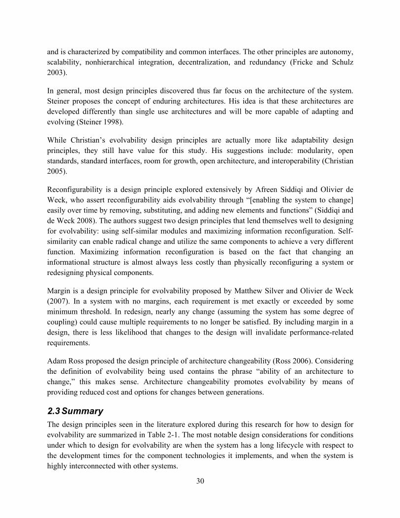
2.3 Summary

The design principles seen in the literature explored during this research for how to design for evolvability are summarized in Table 2-1. The most notable design considerations for conditions under which to design for evolvability are when the system has a long lifecycle with respect to the development times for the component technologies it implements, and when the system is highly interconnected with other systems.

31

Table 2-1. Existing Design Principles for Evolvability

Design Principle Proposed by Modularity Holtta-Otto (2005), Hansen (2003), Christian (2005), Integrability/Common Interfaces Fricke and Schulz (2003), Christian (2005), Holtta-Otto (2005) Interoperability Christian (2005) Scalability Fricke and Schulz (2003) Reconfigurability Siddiqi and de Weck (2008) Margin Christian (2005), Silver and de Weck (2007) Architecture Changeability Ross (2006)

The following chapters will explore methods and metrics that aim to both validate the design principles seen in Table 2-1 and deduct new design principles through application of methods and metrics to case studies.

32

33

3 Developing and Applying Metrics for Evolvability In an ideal world, a system’s evolvability could be measured unambiguously, objectively, and in a repeatable fashion. Given the same information about a set of designs, multiple analysts should be able to reach the same conclusions about the relative evolvability of the set of designs. An evolvability metric is in essence a measure of effectiveness for how well a system can evolve. A measure of effectiveness is “a quantitative expression of how well the operation of a system contributes to the success of the greater system” (Parnell et al. 2008). The “greater system” is the lifecycle of the system, whereas the first reference to “system” in the definition refers to the initial design of the system. How well the system operates is the ease with which the initial design can change its architecture between generations with inheritance. This research seeks to find a suitable metric for evolvability so that such analysis is possible.

3.1 Evaluating Existing Metrics

Since the definitions of evolvability, changeability, flexibility, among others, overlap so often in the literature, the scope of this metric search will expand beyond metrics explicitly for evolvability. One researcher’s evolvability metric might actually measure reconfigurability, while another researcher’s adaptability metric might actually measure evolvability.

3.1.1 Metric Criteria

In order to evaluate the “goodness” of candidate metrics, a set of criteria must be established. Many of the metrics that are examined are characterized by their construct just as much as the actual equation(s) relating to evolvability. Accordingly, the criteria will also evaluate the validity of any associated constructs. A preliminary set of metric criteria is proposed by John Christian (2004) based on the NASA Systems Engineering Handbook and the SMC Systems Engineering Primer and Handbook. Christian proposes that a good metric should:

1. Relate to performance 2. Be simple to state 3. Be complete 4. State any time dependency 5. State any environmental conditions 6. Be quantitative 7. Be easy to measure 8. Help the user identify a system that best meets their objective (in this case: “be

evolvable”) Since the goal is to establish a repeatable metric that leads to valuable insights, the most important considerations from this list are that the metric be quantitative and useful to the user. To be useful to a user, the metric should be relatively easy to implement and exist in a familiar framework. Recall the definition of evolvability being used in this research: “the ability of an

34

architecture to be inherited and changed across generations (over time).” In accordance with the first criterion, “relate to performance”, an evolvability metric must relate to a system’s ability to change its architecture. Ability to change can be viewed as both extent and ease of change. The time-dependency in the case of evolvability is the concept of a generation, which should be considered in a comprehensive evolvability metric. The set of criteria for evaluating evolvability metrics, informed by Christian’s criteria and the definition of evolvability in use, are:

Are time/generations accounted for? o Yes or No

Is the extent of change measured? o None – Extent of change is not considered o Low – Extent of change is measured implicitly o High – The extent of change is explicitly measured

Is the ease of change measured? o None – Ease of change is not considered o Low – Ease of change is measured generally o High - Ease of change is measured for each end state

Is the metric relatively simple to implement? o No – The metric is prohibitively complex and would require extensive work to

implement o Somewhat – The metric is not trivial, but most engineers could apply it given

enough time o Yes – The metric is simple enough that a layperson could apply it and

understand the results with little to no explanation

How accessible is the metric? o New – The metric operates in a new and complex framework not available to

other engineers o Somewhat – The metric operates in a framework that might not be

commonplace, but is understandable and available to other engineers o Very – The metric operates in a framework completely accepted and widely

used by other engineers

These criteria are used to evaluate candidate metrics and inform the choice of the evolvability metrics that will ultimately be tested. Where appropriate, suggestions about how a metric might be modified to better measure evolvability are made. These modifications are considered for the scores that are recorded in the table for each metric.

35

3.1.2 Candidate Metrics

3.1.2.1 Interface Complexity Metric (Holtta-Otto 2005)

The interface complexity metric proposed by Holtta-Otto (2005) was meant to be used to decide where modular boundaries (and therefore interfaces) should be defined in a given system. The metric expresses the relative difficulty of a given change to an interface, measured in percentage of original design effort, as a function of the percent change needed. An example of this relationship is shown in Figure 3-1.

Figure 3-1. Interface Complexity Metric (adapted from Holtta-Otto 2005)

The three parts of the curve, as separated by the two discontinuities on the graph, represent three categories of redesign: (1) where no redesign is required, (2) where redesign is required and some relationship, not necessarily linear, relates the percent change to the redesign effort required, and (3) where the amount of change required is so great that a new module, component, or interface must be acquired or designed. The shortcoming of this metric is that it, as implemented by Holtta-Otto, relies on interviews to develop the relationships. To make this metric more viable, a more robust method of determining these relationships should be developed. Another way to adapt this metric to make it more useful for measuring evolvability would be to use it to measure cost and time required given a specific change in a parameter (as opposed to an interface).

36

Table 3-1. Metric Scores for Interface Complexity Metric

Criteria Score Comments Time/Generations No Potentially captured in “redesign effort” Extent of Change Low In a scalable sense, but only for a single parameter/interface Ease of Change High “Redesign effort” is a measure of ease of change Simple? Somewhat Not complex, but time-intensive by means of interviews Accessible? Somewhat Easy to understand, but not comprehensive of whole system

3.1.2.2 Ontological Approach (Rowe and Leaney 1997)

Rowe and Leaney (1997) propose an ontological framework that fully defines the possible state space, the state functions (Fi), and reference frame of a system. They define a lawful state space as well, which is a subset of the possible state space determined by the laws of physics and other restrictions imposed on the system. Based on this framework, they define the relative change of a system in the ith respect and with respect to α, Vi, to be

i

ii

F

FV

1

These authors propose interpreting the relative rate of change as the sensitivity of an architecture to changes in particular requirements that affect system properties. They also define the relative extent of change of a system in the ith respect, with respect to α over the interval [α1, α2] to be

12

12

1221

)(ln)(ln

1),(

2

1

ii

ii

FF

V

They propose interpreting the relative extent of change as the normalized effort required to perform a given change. Both of these measures would contribute to measuring evolvability; the only drawback to this framework is that it requires the system designer to have a very well-defined and extensive model of the system, including all of its state functions in terms of all system parameters. An improvement on these metrics would be to add a cost function that could be combined, especially with the relative extent of change, to represent the cost of a given change. If the user defines a cost threshold, these metrics could then be used to explore the tradespace to see what subset is reachable with the given resources.

37

Table 3-2. Metric Scores for Ontological Approach

Criteria Score Comments Time/Generations No Not stated Extent of Change High Explicitly measured Ease of Change High Explicitly measured Simple? No Not simple to implement due to the nature of the framework Accessible? Somewhat Requires extensively-defined, but accepted, framework

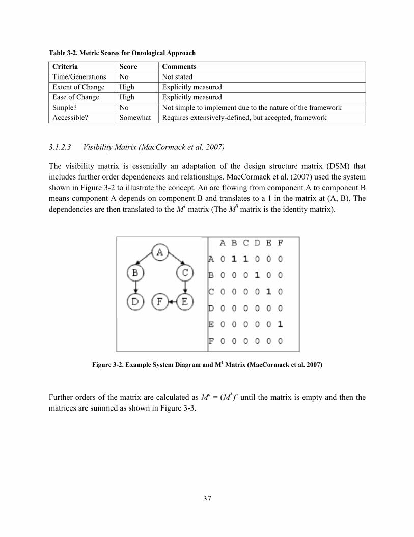
3.1.2.3 Visibility Matrix (MacCormack et al. 2007)

The visibility matrix is essentially an adaptation of the design structure matrix (DSM) that includes further order dependencies and relationships. MacCormack et al. (2007) used the system shown in Figure 3-2 to illustrate the concept. An arc flowing from component A to component B means component A depends on component B and translates to a 1 in the matrix at (A, B). The dependencies are then translated to the M1 matrix (The M0 matrix is the identity matrix).

Figure 3-2. Example System Diagram and M1 Matrix (MacCormack et al. 2007)

Further orders of the matrix are calculated as Mn = (M1)n until the matrix is empty and then the matrices are summed as shown in Figure 3-3.

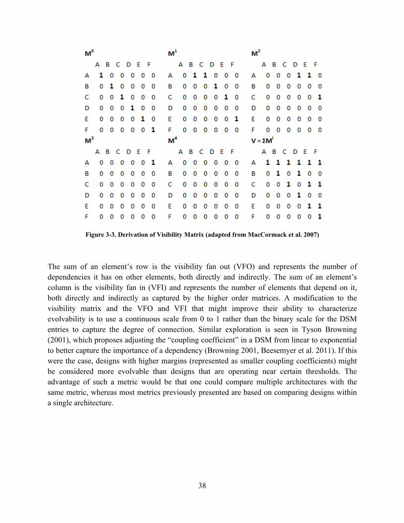
38

Figure 3-3. Derivation of Visibility Matrix (adapted from MacCormack et al. 2007)

The sum of an element’s row is the visibility fan out (VFO) and represents the number of dependencies it has on other elements, both directly and indirectly. The sum of an element’s column is the visibility fan in (VFI) and represents the number of elements that depend on it, both directly and indirectly as captured by the higher order matrices. A modification to the visibility matrix and the VFO and VFI that might improve their ability to characterize evolvability is to use a continuous scale from 0 to 1 rather than the binary scale for the DSM entries to capture the degree of connection. Similar exploration is seen in Tyson Browning (2001), which proposes adjusting the “coupling coefficient” in a DSM from linear to exponential to better capture the importance of a dependency (Browning 2001, Beesemyer et al. 2011). If this were the case, designs with higher margins (represented as smaller coupling coefficients) might be considered more evolvable than designs that are operating near certain thresholds. The advantage of such a metric would be that one could compare multiple architectures with the same metric, whereas most metrics previously presented are based on comparing designs within a single architecture.

39

Table 3-3. Metric Scores for Visibility Matrix

Criteria Score Comments Time/Generations No Not stated Extent of Change None Specific changes are not examined Ease of Change Low VFO and VFI scores map “ease” to amount of propagation Simple? Yes Once the DSM exists, very simple calculation Accessible? Yes DSM is a familiar framework for many engineers

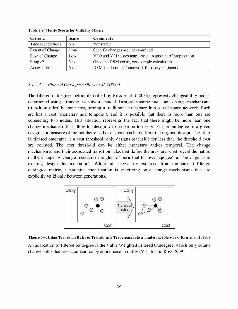
3.1.2.4 Filtered Outdegree (Ross et al. 2008b)

The filtered outdegree metric, described by Ross et al. (2008b) represents changeability and is determined using a tradespace network model. Designs become nodes and change mechanisms (transition rules) become arcs, turning a traditional tradespace into a tradespace network. Each arc has a cost (monetary and temporal), and it is possible that there is more than one arc connecting two nodes. This situation represents the fact that there might be more than one change mechanism that allow for design X to transition to design Y. The outdegree of a given design is a measure of the number of other designs reachable from the original design. The filter in filtered outdegree is a cost threshold; only designs reachable for less than the threshold cost are counted. The cost threshold can be either monetary and/or temporal. The change mechanisms, and their associated transition rules that define the arcs, are what reveal the nature of the change. A change mechanism might be “burn fuel to lower apogee” or “redesign from existing design documentation”. While not necessarily excluded from the current filtered outdegree metric, a potential modification is specifying only change mechanisms that are explicitly valid only between generations.

Figure 3-4. Using Transition Rules to Transform a Tradespace into a Tradespace Network (Ross et al. 2008b)

An adaptation of filtered outdegree is the Value Weighted Filtered Outdegree, which only counts change paths that are accompanied by an increase in utility (Viscito and Ross 2009).

40

Table 3-4. Metric Scores for Filtered Outdegree

Criteria Score Comments Time/Generations Yes Both in arc definition and potentially in transition rule Extent of Change High Specific changes are counted Ease of Change High Ease of change is captured in the threshold filter Simple? Yes The calculations are simple Accessible? Somewhat Design space must be defined using a specific basis

3.1.3 Selecting the Metric: Filtered Outdegree for Evolvability

The overall set of candidate metric scores is captured in Table 3-5. Only one metric, the filtered outdegree, takes time and generations into account at all. Most of the metrics do a good job of evaluating ease of change, but there is more variance in how well they evaluate extent of change. Filtered outdegree and the ontological approach were the only metrics to score a “high” in both extent and ease of change categories. Varying degrees of simplicity and accessibility were seen, with only the visibility matrix scoring highest marks in both categories. Looking back to the two metrics that best evaluated ease and extent of change, only filtered outdegree lacked “no” scores.

Table 3-5. Overview of Metric Scores

Metric Time/Generations Extent Ease Simple? Accessible?

Interface Complexity Metric No Low High Somewhat Somewhat

Ontological Approach No High High No Somewhat

Visibility Matrix No None Low Yes Yes

Filtered Outdegree Yes High High Yes Somewhat

The filtered outdegree metric received top marks in four out of five categories and a medium score in the fifth category. No other metric evaluated came close to this, and thus the filtered outdegree is the metric that is used for measuring evolvability. The metric is modified from its form in Ross et al. (2008) to only include change mechanisms that are in line with the definition of evolvability. The formal definition for the chosen metric is: the filtered outdegree for

evolvability of a design, FOE(< ), is the number of designs reachable for less than threshold

cost using only evolvable transition rules.

3.2 Application to Space Tug The following section explores the application of the selected metric, filtered outdegree for evolvability, to the Space Tug case study. The Space Tug case study contains designs for orbital transfer vehicles that can be used for a variety of on-orbit servicing missions such as observation of (potentially hostile) targets, assisting in orbit changes, and removing debris (McManus and Schuman 2003). This data set has been used for studies in changeability and survivability (Richards 2009, Ross and Hastings 2006). Recent work has added context variables to the

41

existing preference curves used to define the epochs. Applying the metric to case studies has two concurrent purposes: identify evolvable designs and motivate design principles for evolvability. Evolvable designs are identified by their high metric scores, and the commonalities between these designs will inform additional design considerations and insights as to why they are evolvable, ideally leading to design principles.

3.2.1 Tradespace Definition

A tradespace is the collection of enumerated designs that can specify a system. The tradespace is defined by the design variables it contains and the levels each design variable may take. For the Space Tug case study, the design variables originally introduced include manipulator size, propulsion system, and fuel mass (McManus and Schuman 2003). An additional variable, design for evolvability (DfE), was added for the purposes of this research. The DfE variable represents the inclusion of design heuristics that make redesign simpler and is treated as a mass penalty. The ranges of values for the design variables are seen in Table 3-6. The enumerated tradespace based on these variable levels contains 256 designs.

Table 3-6. Design Variable Levels (modified from McManus and Schuman 2003)

Design Variables Levels Architecture Variable?

Manipulator Mass (kg) [300, 1000, 3000, 5000] No Fuel Mass (kg) [30, 100, 300, 600, 1200, 3000, 10000, 30000] No Propulsion System Storable Bipropellant, Cryogenic, Electric, Nuclear Yes DfE (% Mass Penalty) [0, 20] Yes

Table 3-7 shows the intermediate variables associated with each propulsion system that are used in calculating wet and dry mass values. The cost of a design is a function of its dry and wet mass. First, the propulsion system mass (Mp) must be calculated using base mass (mp0), mass fraction (mpf), and the fuel mass (Mf)

fpfpp MmmM 0

Base mass and mass fraction values for a specific propulsion system may be found in Table 3-7.

Table 3-7. Propulsion System Values (McManus and Schuman 2003)

Propulsion System Base Mass (kg) Mass Fraction Storable Bipropellant 0 0.12 Cryogenic 0 0.13 Electric 25 0.25 Nuclear 1000 0.20

Next, the vehicle bus mass (Mb) is calculated using the propulsion system mass, manipulator mass (Mm), and bus mass fraction (mbf)

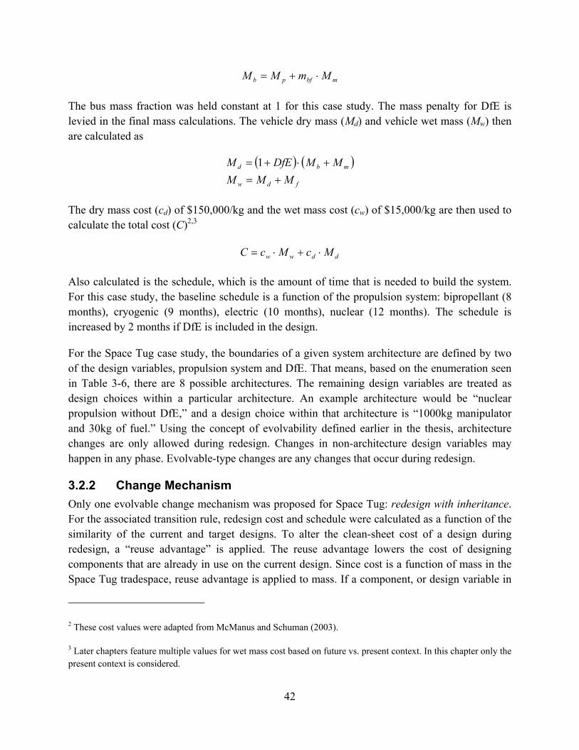
42

mbfpb MmMM

The bus mass fraction was held constant at 1 for this case study. The mass penalty for DfE is levied in the final mass calculations. The vehicle dry mass (Md) and vehicle wet mass (Mw) then are calculated as

fdw

mbd

MMM

MMDfEM

1

The dry mass cost (cd) of $150,000/kg and the wet mass cost (cw) of $15,000/kg are then used to calculate the total cost (C)2,3

ddww McMcC

Also calculated is the schedule, which is the amount of time that is needed to build the system. For this case study, the baseline schedule is a function of the propulsion system: bipropellant (8 months), cryogenic (9 months), electric (10 months), nuclear (12 months). The schedule is increased by 2 months if DfE is included in the design.

For the Space Tug case study, the boundaries of a given system architecture are defined by two of the design variables, propulsion system and DfE. That means, based on the enumeration seen in Table 3-6, there are 8 possible architectures. The remaining design variables are treated as design choices within a particular architecture. An example architecture would be “nuclear propulsion without DfE,” and a design choice within that architecture is “1000kg manipulator and 30kg of fuel.” Using the concept of evolvability defined earlier in the thesis, architecture changes are only allowed during redesign. Changes in non-architecture design variables may happen in any phase. Evolvable-type changes are any changes that occur during redesign.

3.2.2 Change Mechanism

Only one evolvable change mechanism was proposed for Space Tug: redesign with inheritance. For the associated transition rule, redesign cost and schedule were calculated as a function of the similarity of the current and target designs. To alter the clean-sheet cost of a design during redesign, a “reuse advantage” is applied. The reuse advantage lowers the cost of designing components that are already in use on the current design. Since cost is a function of mass in the Space Tug tradespace, reuse advantage is applied to mass. If a component, or design variable in

2 These cost values were adapted from McManus and Schuman (2003).

3 Later chapters feature multiple values for wet mass cost based on future vs. present context. In this chapter only the present context is considered.

43

the context of the Space Tug data set, is changed, the full component mass is used to calculate the cost. If a component does not change, its mass is reduced by the reuse advantage. If DfE is not included in the original design, the reuse advantage is zero. For this case study, if DfE is included, the reuse advantage is 50%.

Redesign schedule (Sij) is a function of the new propulsion system, current DfE level (DfEi), and target DfE level (DfEj). A depiction of what redesign schedule means can be seen in Figure 3-5.

Figure 3-5. Depiction of Redesign Schedule

The baseline schedule (Si) is the same as in the original design, based on propulsion system. If the previous design included DfE, an evolvability advantage (EA) is subtracted from the schedule. [Note all DfE variables are binary for these equations4]

EPDfEEADfESS addediiij **

Where

ijadded DfEDfEDfE 1

4 The DfE variables are binary here for the purposes of the schedule equations only. Since the actual DfE percentage is used in the mass calculations, making the variable binary was not an option. These schedule equations are therefore only valid for the case of two DfE levels. As the number of DfE levels expands beyond two, schedule equations will need to be revisited. Here a DfE mass penalty of 0% corresponds to 0 and 20% corresponds to 1.

44

EA = 3 months

EP = 2 months

In this case study, the evolvability advantage was 3 months, meaning the evolvable redesign process takes 3 months less time than that of a clean-sheet development of the same design. If DfE was not included in the original design but is to be included in the new design, the same 2 month evolvability penalty (EP) is applied. This penalty is not applied for continuing to have DfE (i.e., both the original and new design include DfE).

3.2.3 Results: Calculation of Filtered Outdegree

The first set of plots, seen in Figure 3-6, look at the entire tradespace. Each plot was generated using a different, but constant cost threshold used in the calculation of outdegree (at $300M, $600M, $900M, $1200M, $1500M, and $4000M, respectively). The fact that filtered outdegree as a function of cost is a non-decreasing function is clear; the filtered outdegree for a given design never decreases with an increase in cost. As the cost threshold grows, the filtered outdegree of every design approaches 224. This value is the difference between the size of the full tradespace, 256, and the number of designs that share the same architecture, 32 (including the original design). Notice that the 4-color pattern repeats 4 times as design number increases; each repetition is for a different manipulator mass, increasing from left to right. The 8 points in each color band represent the 8 different fuel levels. The final variable, DfE, is manifested in the two different lines. Since DfE will never make a transition more expensive, the “with DfE” value of filtered outdegree will never be below the corresponding “without DfE” value.

Many observations can be drawn from these graphs. The red and black color bands, (corresponding to nuclear propulsion and electric propulsion, respectively) are never below the blue and green color bands (corresponding to nuclear propulsion and electric propulsion, respectively). This can be attributed to the fact that only nuclear propulsion and electric propulsion systems have base masses associated with them. An example can be used to better understand this behavior. System A and B have the same manipulator size (1000kg), fuel level (600kg), and include DfE. System A has a storable bipropellant propulsion whereas System B has a nuclear propulsion system. The arcs connection System A or System B to any system with cryogenic or electric propulsion will have exactly the same transition cost. The cryogenic and electric component of the filtered outdegree value is identical for System A and System B. The transition from System A to System B, however, is more expensive than from System B to System A. This is due to the fact that the propulsion mass cost is higher for System B due to the 1000kg base mass associated with nuclear propulsion. The A-B transition incurs this cost, whereas the B-A transition only incurs the mass fraction costs.

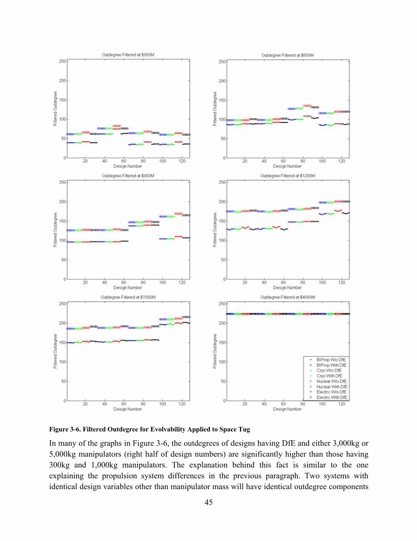
45

Figure 3-6. Filtered Outdegree for Evolvability Applied to Space Tug

In many of the graphs in Figure 3-6, the outdegrees of designs having DfE and either 3,000kg or 5,000kg manipulators (right half of design numbers) are significantly higher than those having 300kg and 1,000kg manipulators. The explanation behind this fact is similar to the one explaining the propulsion system differences in the previous paragraph. Two systems with identical design variables other than manipulator mass will have identical outdegree components

46

to the other two manipulator masses. However, the transition to the larger manipulator mass are more expensive than the transition to the smaller manipulator mass.

Another way to look at the data is to see how a specific architecture variable affects filtered outdegree. Figure 3-7 shows the filtered outdegree distributions for designs 164, 172, 180, and 188 as a function of cost threshold. Each design has a 1,000kg manipulator, 600kg of fuel, and includes DfE. The four curves shown are for the four different propulsion systems. A zoomed in view is shown to give an idea of how close the filtered outdegree values can be for a specific cost; the values are rarely separated by more than 10. The relative closeness of the four curves insinuates that propulsion system does not have a strong influence on filtered outdegree for this set of design variables, meaning DfE is the only architecture variable with an influence on evolvability for the Space Tug case study.

Figure 3-7. Filtered Outdegree of a Design for Different Propulsion systems (Transition Cost on x-axis)

Manipulator mass appears to have a more significant impact on filtered outdegree, as seen in Figure 3-8. This is largely due to the fact that the reuse advantage is only applied to manipulator mass when the original design and transition design have the same size manipulator. The savings from evolvability (DfE) then are proportional to the size of the original manipulator. A design with a 5,000kg manipulator saves $375M using evolvable redesign whereas a design with a

47

300kg manipulator only saves $22.5M. This is an intriguing insight because we see that a non-architecture design variable level can impact the evolvability of the system. This could mean that the level of a design variable can influence the architecture and therefore affect evolvability (e.g. the fuel mass impacts the architecture through the fuel mass fraction equation). While not pictured, analysis showed that fuel mass had very little impact on filtered outdegree. This is due to the order of magnitude difference in wet mass cost and dry mass cost.

Figure 3-8. Filtered Outdegree of a Design for Different Manipulator Masses

An additional way to use filtered outdegree to analyze design alternatives is to compare the filtered outdegree of a design with and without a specific option while accounting for the cost of including that option, heretofore referred to as adjusted filtered outdegree. An example of adjusted filtered outdegree applied to the DfE variable for Space Tug can be seen in Figure 3-9. The cost filter used in calculating the adjusted outdegree for the design including DfE takes into account the cost of including DfE (calculated as Cost[Design X with DfE] – Cost [Design X without DfE]). For Design 1, the DfE cost is approximately $10M. For every cost threshold, the adjusted filtered outdegree of the design with DfE included was higher than the design that did not include DfE. This is not always the case, however. Design 100, seen in Figure 3-10, exhibits a higher adjusted filtered outdegree than its corresponding design with DfE until a cost threshold of $690M. The DfE cost for Design 100 was $166M, which means that FOE

228($690M - $166M = $524M) is approximately equal to FOE

100($690M). A designer or stakeholder can interpret this

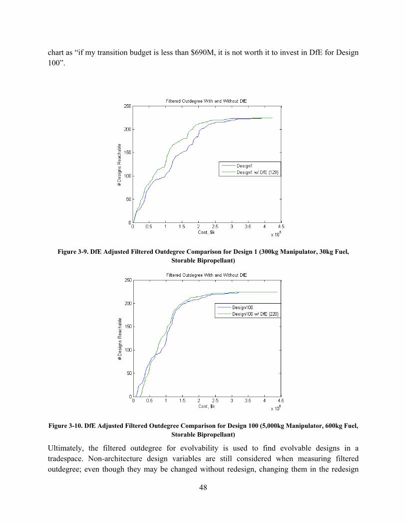
48

chart as “if my transition budget is less than $690M, it is not worth it to invest in DfE for Design 100”.

Figure 3-9. DfE Adjusted Filtered Outdegree Comparison for Design 1 (300kg Manipulator, 30kg Fuel, Storable Bipropellant)

Figure 3-10. DfE Adjusted Filtered Outdegree Comparison for Design 100 (5,000kg Manipulator, 600kg Fuel, Storable Bipropellant)

Ultimately, the filtered outdegree for evolvability is used to find evolvable designs in a tradespace. Non-architecture design variables are still considered when measuring filtered outdegree; even though they may be changed without redesign, changing them in the redesign

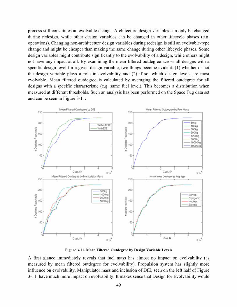
49

process still constitutes an evolvable change. Architecture design variables can only be changed during redesign, while other design variables can be changed in other lifecycle phases (e.g. operations). Changing non-architecture design variables during redesign is still an evolvable-type change and might be cheaper than making the same change during other lifecycle phases. Some design variables might contribute significantly to the evolvability of a design, while others might not have any impact at all. By examining the mean filtered outdegree across all designs with a specific design level for a given design variable, two things become evident: (1) whether or not the design variable plays a role in evolvability and (2) if so, which design levels are most evolvable. Mean filtered outdegree is calculated by averaging the filtered outdegree for all designs with a specific characteristic (e.g. same fuel level). This becomes a distribution when measured at different thresholds. Such an analysis has been performed on the Space Tug data set and can be seen in Figure 3-11.

Figure 3-11. Mean Filtered Outdegree by Design Variable Levels

A first glance immediately reveals that fuel mass has almost no impact on evolvability (as measured by mean filtered outdegree for evolvability). Propulsion system has slightly more influence on evolvability. Manipulator mass and inclusion of DfE, seen on the left half of Figure 3-11, have much more impact on evolvability. It makes sense that Design for Evolvability would

50

increase evolvability; DfE directly impacts transition costs. The reason having a larger manipulator results in a system being more evolvable is not as obvious. It does make sense, however, that making a satellite’s payload smaller should be easier than making it larger. Having the ability to exceed requirements in payload capability is an embodiment of the previously proposed design principle for evolvability, margin. Deliberately oversizing the payload makes it easier to later switch to a smaller payload. For example, assuming a space tug satellite with a 5,000 kg payload has the power and delta V budgets to accomplish its mission, it should also have the budgets to do so with a 300 kg payload. A space tug satellite designed around a 300 kg might not have the power and delta V capabilities to accomplish the mission with a 5,000 kg manipulator.

Several insights have now been taken from the Space Tug case study related to choosing design and architecture variables to influence evolvability. Having DfE is an architecture level choice that can be made to increase evolvability. Having a large manipulator is a design level choice that increases evolvability. Looking to the mechanics of the transition rule, any process or design improvement that increases the reuse advantage or decreases the evolvability mass penalty would have a positive impact on evolvability. Developing new path enablers that make transitions cheaper or faster will also benefit the evolvability of the system. Process improvements that save time in making evolvable changes between generations (such as team continuity, documentation, etc.) will promote evolvability as well.

3.3 Conclusions

The state of evolvability metrics prior to this research was disjointed. By comparing existing metrics against a set of criteria informed by the definition of evolvability used in this research thread, the filtered outdegree for evolvability was selected and modified to best measure evolvability. By establishing a metric for evolvability, design principle investigation is possible for a given case study by means of comparing designs with high evolvability scores. As a result of applying filtered outdegree to the Space Tug case study, margin was identified as a design principle for evolvability, specifically in the payload mass variable.

51

4 Epoch Syncopation Framework

4.1 Overview This section explores the motivation for the Epoch Syncopation Framework, existing methods, and the architecture of the framework.

4.1.1 Motivation

Decisions early in the design process, especially in the conceptual design phase, require careful consideration as they will ultimately enable or limit the success of the system. If a system is not designed to robustly perform across shifting epochs (a period of fixed contexts and expectations), the system can be designed to change in response to these shifts in order to retain useful functionality and avoid suffering deficiencies or even failure. A system can incorporate changeability, the ability to change its form, function, or operations, including evolvability, the ability to change its architecture between generations with inheritance, as ways to dynamically react to changing epochs (Ross and Hastings 2006, Beesemyer, Fulcoly et al. 2011). Changeability looks at all change mechanisms available to a system and how they increase the number of reachable states in the tradespace, or set of designs considered, available to the current design state (Ross 2006). Designing an evolvable system may reduce the long term cost of system upgrades or replacements in the presence of epoch shifts over its lifespan (Beesemyer et al. 2011). Executing change mechanisms, including redesigning a system, can be an expensive process. Additionally, if an epoch shift occurs shortly after or even during the execution of a change mechanism, the change can have less positive, or potentially negative consequences; deliberate and syncopated timing of change mechanism executions can potentially reduce cost and increase the benefit to system stakeholders. Choosing change strategies and time constants based on knowledge of epoch variables can improve the timing of change mechanism executions, similar to the idea of a “battle rhythm” proposed in (Dahmann et al. 2010). The Epoch Syncopation Framework (ESF) is introduced here as a way of analyzing point designs, change mechanisms, execution timing, and change strategies.

4.1.2 Prior Methods

The ESF is not the first method to analyze tradespaces in the context of entire eras (time ordered sequence of epochs). The ESF was derived from an earlier framework, the Technology Syncopation Framework (TSF) created by the same authors (Beesemyer et al. 2011). The TSF was essentially an abstracted version of the ESF, but its abstraction was ultimately its weakness as it did not consider actual design variables and epoch variables. A similar method to the ESF, the Time-Expanded Decision Network (TDN), was developed in (Silver and de Weck 2007). The TDN can be very useful on its own, but the ESF makes some useful improvements to enable the inclusion of more change strategies.

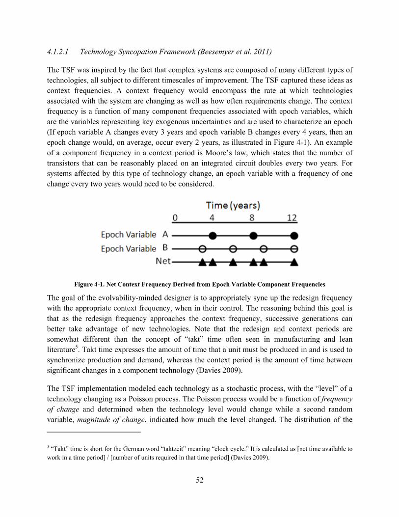
52

4.1.2.1 Technology Syncopation Framework (Beesemyer et al. 2011)

The TSF was inspired by the fact that complex systems are composed of many different types of technologies, all subject to different timescales of improvement. The TSF captured these ideas as context frequencies. A context frequency would encompass the rate at which technologies associated with the system are changing as well as how often requirements change. The context frequency is a function of many component frequencies associated with epoch variables, which are the variables representing key exogenous uncertainties and are used to characterize an epoch (If epoch variable A changes every 3 years and epoch variable B changes every 4 years, then an epoch change would, on average, occur every 2 years, as illustrated in Figure 4-1). An example of a component frequency in a context period is Moore’s law, which states that the number of transistors that can be reasonably placed on an integrated circuit doubles every two years. For systems affected by this type of technology change, an epoch variable with a frequency of one change every two years would need to be considered.

Figure 4-1. Net Context Frequency Derived from Epoch Variable Component Frequencies

The goal of the evolvability-minded designer is to appropriately sync up the redesign frequency with the appropriate context frequency, when in their control. The reasoning behind this goal is that as the redesign frequency approaches the context frequency, successive generations can better take advantage of new technologies. Note that the redesign and context periods are somewhat different than the concept of “takt” time often seen in manufacturing and lean literature5. Takt time expresses the amount of time that a unit must be produced in and is used to synchronize production and demand, whereas the context period is the amount of time between significant changes in a component technology (Davies 2009).

The TSF implementation modeled each technology as a stochastic process, with the “level” of a technology changing as a Poisson process. The Poisson process would be a function of frequency of change and determined when the technology level would change while a second random variable, magnitude of change, indicated how much the level changed. The distribution of the

5 “Takt” time is short for the German word “taktzeit” meaning “clock cycle.” It is calculated as [net time available to work in a time period] / [number of units required in that time period] (Davies 2009).

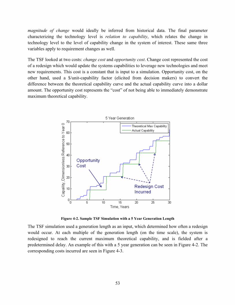
53

magnitude of change would ideally be inferred from historical data. The final parameter characterizing the technology level is relation to capability, which relates the change in technology level to the level of capability change in the system of interest. These same three variables apply to requirement changes as well.

The TSF looked at two costs: change cost and opportunity cost. Change cost represented the cost of a redesign which would update the systems capabilities to leverage new technologies and meet new requirements. This cost is a constant that is input to a simulation. Opportunity cost, on the other hand, used a $/unit-capability factor (elicited from decision makers) to convert the difference between the theoretical capability curve and the actual capability curve into a dollar amount. The opportunity cost represents the “cost” of not being able to immediately demonstrate maximum theoretical capability.

Figure 4-2. Sample TSF Simulation with a 5 Year Generation Length

The TSF simulation used a generation length as an input, which determined how often a redesign would occur. At each multiple of the generation length (on the time scale), the system is redesigned to reach the current maximum theoretical capability, and is fielded after a predetermined delay. An example of this with a 5 year generation can be seen in Figure 4-2. The corresponding costs incurred are seen in Figure 4-3.

54

Figure 4-3. Costs Corresponding to the TSF Simulation seen in Figure 4-2

Ultimately, the TSF was used to explore how generation length could be chosen based on an opportunity cost factor and the change parameters of input technologies and requirements. While the results were limited, there did appear to be a trend that choosing a redesign frequency close to the change frequency of the input technology with the greatest mean magnitude of change resulted in the lowest total cost.

4.1.2.2 Time-Expanded Decision Networks (Silver and de Weck 2007)

The TDN is a method created to “design and analyze flexibility in large-scale complex systems.” The method is divided into five steps: “(1) Design a set of potential system configurations; (2) quantify switching costs to create a “static network” that captures the difficulty of switching among these configurations; (3) create a time-expanded decision network by expanding the static network in time, including chance and decision nodes; (4) evaluate minimum cost paths through the network under plausible operating scenarios; and (5) modify the set of initial design configurations to exploit high-leverage switches and repeat the process to convergence.” Costs in the TDN consist of explicit non-recurring costs, fixed recurring costs, and variable recurring costs. Switching costs are broken into a technical cost and an organizational premium. Technical costs include the cost of retiring the old system and designing the new system. The switching costs are used to generate the static network, with source and sink nodes representing the original fielding and final retirement. The static network becomes a time-expanded network when chance and decision nodes are added. The arcs connecting designs gain a time component in addition to the switching cost already associated with them. The time-expanded network, with chance nodes represented as circles and decision nodes represented as squares, can be seen in Figure 4-4. In

55

creating scenarios to optimize, the authors suggest using geometric Brownian motion to apply multiple combinations of demand scenarios, or simply choosing a few representative cases to test for. The cost of operating in each time period is a function of the demand scenario and the current state of the system. While the optimization records all information about how the system traverses through the time period, the information of most interest is the configurations that were chosen first most often and the switches that were implemented the most. The final step in the process is to use it in a multitude of scenarios in order to identify the point designs and interfaces that can help lower costs. This analysis can also shed light on opportunities to embed real options.

Figure 4-4. Visualization of the TDN (Silver and de Weck 2007)

A significant limitation of the TDN approach is the fact that the TDN only considers uncertainty in demand. While this might be sufficient for some analyses, as the scope of analysis widens it becomes important to analyze the uncertainty of all variables. A second shortcoming of the TDN is the mandatory coupling of uncertainty nodes and decision nodes. Many decisions are in fact reactions to changes in context variables, but excluding the possibility of proactive change behavior is not beneficial for widening the scope of change strategy analysis; a change behavior that was independent of changes in context would not be possible in the TDN approach.

4.1.2.3 Decision Tree Analysis and Binomial Lattice Models (Cardin 2011)

Decision tree analysis and lattice models are techniques for analyzing real options for flexibility in an engineering system. These methods use economic metrics such as net present value (NPV) and uncertainty models to estimate the value of a flexible option. For decision tree analysis, the time-evolution of uncertainty is represented using a decision tree structure. Much like the TDN method, after each uncertainty node (circle nodes in Figure 4-5) a decision node (square nodes in

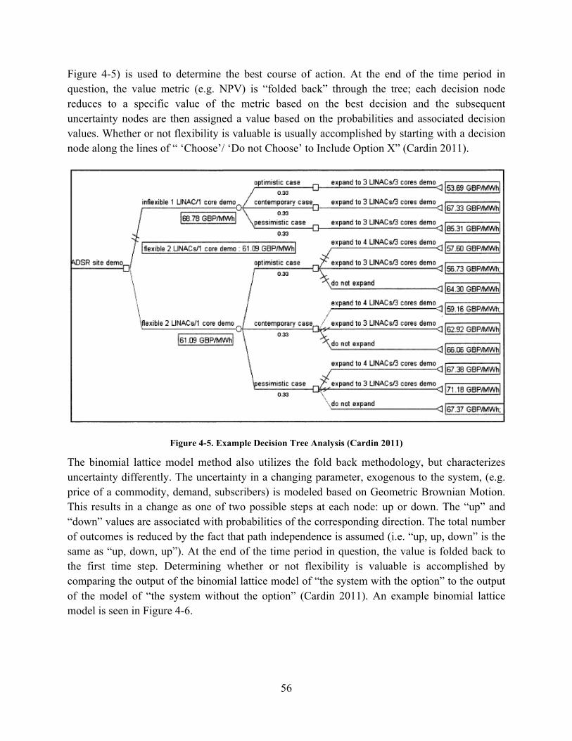
56

Figure 4-5) is used to determine the best course of action. At the end of the time period in question, the value metric (e.g. NPV) is “folded back” through the tree; each decision node reduces to a specific value of the metric based on the best decision and the subsequent uncertainty nodes are then assigned a value based on the probabilities and associated decision values. Whether or not flexibility is valuable is usually accomplished by starting with a decision node along the lines of “ ‘Choose’/ ‘Do not Choose’ to Include Option X” (Cardin 2011).

Figure 4-5. Example Decision Tree Analysis (Cardin 2011)

The binomial lattice model method also utilizes the fold back methodology, but characterizes uncertainty differently. The uncertainty in a changing parameter, exogenous to the system, (e.g. price of a commodity, demand, subscribers) is modeled based on Geometric Brownian Motion. This results in a change as one of two possible steps at each node: up or down. The “up” and “down” values are associated with probabilities of the corresponding direction. The total number of outcomes is reduced by the fact that path independence is assumed (i.e. “up, up, down” is the same as “up, down, up”). At the end of the time period in question, the value is folded back to the first time step. Determining whether or not flexibility is valuable is accomplished by comparing the output of the binomial lattice model of “the system with the option” to the output of the model of “the system without the option” (Cardin 2011). An example binomial lattice model is seen in Figure 4-6.

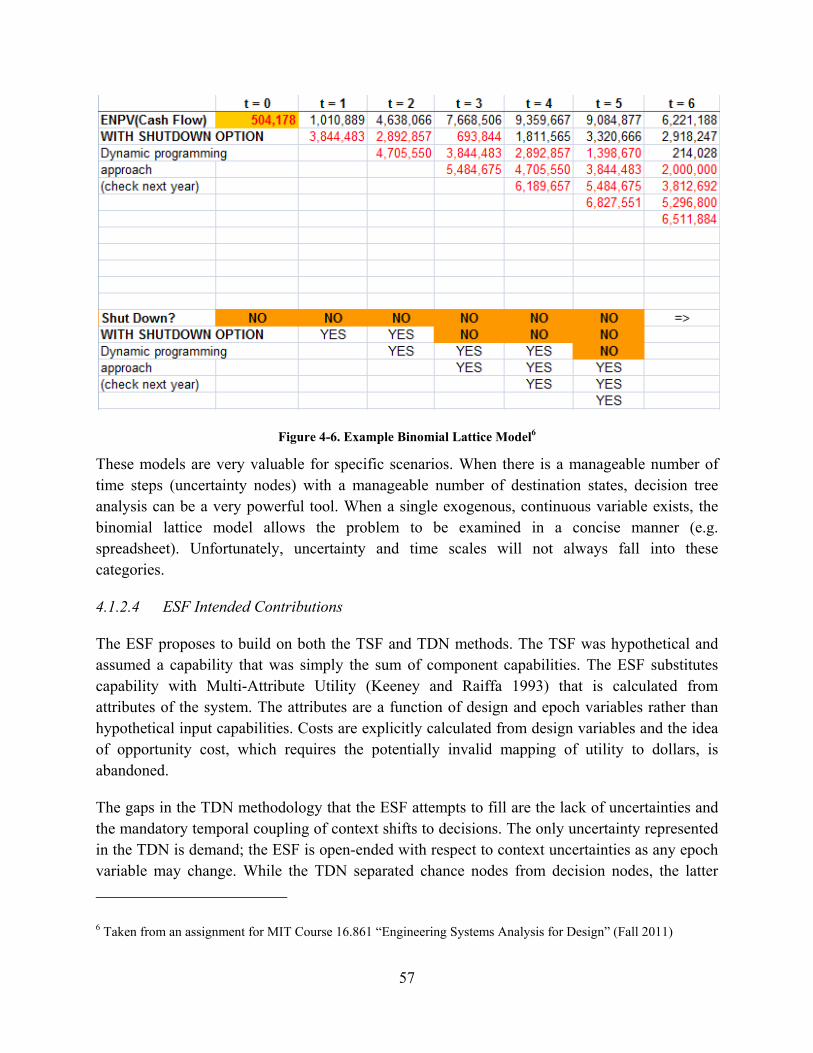
57

Figure 4-6. Example Binomial Lattice Model6

These models are very valuable for specific scenarios. When there is a manageable number of time steps (uncertainty nodes) with a manageable number of destination states, decision tree analysis can be a very powerful tool. When a single exogenous, continuous variable exists, the binomial lattice model allows the problem to be examined in a concise manner (e.g. spreadsheet). Unfortunately, uncertainty and time scales will not always fall into these categories.

4.1.2.4 ESF Intended Contributions

The ESF proposes to build on both the TSF and TDN methods. The TSF was hypothetical and assumed a capability that was simply the sum of component capabilities. The ESF substitutes capability with Multi-Attribute Utility (Keeney and Raiffa 1993) that is calculated from attributes of the system. The attributes are a function of design and epoch variables rather than hypothetical input capabilities. Costs are explicitly calculated from design variables and the idea of opportunity cost, which requires the potentially invalid mapping of utility to dollars, is abandoned.

The gaps in the TDN methodology that the ESF attempts to fill are the lack of uncertainties and the mandatory temporal coupling of context shifts to decisions. The only uncertainty represented in the TDN is demand; the ESF is open-ended with respect to context uncertainties as any epoch variable may change. While the TDN separated chance nodes from decision nodes, the latter

6 Taken from an assignment for MIT Course 16.861 “Engineering Systems Analysis for Design” (Fall 2011)

58

always immediately followed the former. The ESF does not require a decision to change immediately follow a change in context, even though it often will. This change was crucial in order to allow examination of the generational redesign strategy.

While valuable for specific uncertainty scenarios, the ESF aims to be more broadly applicable than decision tree analysis and binomial lattice models. Both methods also had the same shortcoming as the TDN with respect to coupling uncertainty and decision nodes.

4.1.3 ESF Architecture

The computational implementation of the ESF can be seen in Figure 4-7; rectangular text boxes represent objects (vector, matrix, algorithm, etc.) while elliptical text boxes represent processes. The key inputs of the ESF are on the left side of the figure: epoch variables and their change parameters, the set of designs as well as the initial design the system will take on, the transition matrices between the designs for both schedule and cost, and the change strategy that is used. An additional input to the era simulation is the era, which is created stochastically by the era constructor as a function of the epoch variable change parameters. The outputs for the simulation of that era are three time series: design ID, costs incurred, and utility.

Figure 4-7. Architecture of the ESF

4.2 ESF Process The following sections detail each object and process seen in Figure 4-7. The description of input objects explains the way that tradespace data should be organized so that the ESF may be applied. The era constructor and era simulation processes are abstracted so that they might be applied to any case study by any research group hoping to make use of the ESF.

59

4.2.1 Inputs

4.2.1.1 Epoch Variables and Change Parameters

Each epoch variable subject to change should have two change parameters associated with it: an average duration and a Markov probability transition matrix. The ESF, specifically the era constructor, assumes that epoch variables adhere to the Markov property which asserts that the future state depends only on the current state. While other stochastic models could be used, the use of Poisson events and Markov chains allows for the epoch variables to be considered independently and stationary probabilities to be calculated. Additionally, the initial state of each epoch variable should be defined. More discussion of how exactly these parameters are used in the simulation can be found in 4.2.2. The ESF treats the shifting of an epoch variable as a Poisson event, with the Poisson parameter for a given variable set to the average duration of that variable. The Markov probability transition matrix for a given variable should be an n x n matrix, where n is the number of levels for that epoch variable. An entry in row i, column j, represents the probability that the next state will be j given that the current state is i. In accordance with the Law of Total Probability, the values in each row should sum to unity.

4.2.1.2 Design Transition Matrices

These matrices detail whether or not a transition is possible, how much it will cost, and how long given a current design, target design, a change mechanism, and set of epoch variables. The information conveyed in a transition matrix might be “in Epoch 1, it costs $3M for Design 2 to transition to Design 8 using change mechanism 4 and will take 5 months to complete” or “in Epoch 10, Design 3 may not transition to Design 2 using change mechanism 1.” There are two transition matrices (cost and schedule) for each change mechanism and combination of epoch variables that affects transitions.

4.2.1.3 Design Set and Initial Design

The design set contains all the information pertaining to initial cost and schedule as well as attributes for each design. These values can be a function of epoch variables. Note that utility is not contained in the design set, as it is a function of preference set which is an epoch variable. The initial design is the design that will be in design phase at the beginning of the simulation (i.e. the first design to be fielded after the design and build process is complete).

4.2.1.4 Change Strategies

Change strategies are logic statements that determine when a design change will occur, how it will occur (which change mechanism), and to what design the original design will change to (Fitzgerald & Ross 2012). If a stakeholders know how they plan to change, for example if it is an organizational policy, this might be help constant. In other cases, the stakeholders might want to simulate many different change mechanisms are best for them. Each change strategy can have its

60

own inputs as well, as seen in Table 4-1. Three change strategies are examined in this research: (1) always change to the design with the highest utility possible, (2) change only when utility falls below a certain threshold, and (3) change every X years if utility falls below a certain threshold.

Table 4-1. Inputs for Change Strategies

Strategy Name Inputs 1 Always Seek Highest Utility None 2 Exceed Utility Threshold Threshold Percentile 3 Exceed Utility Threshold at

Generation Intervals Threshold Percentile, Generation Length

The first strategy looks at the current utility and the utility of all reachable designs; if a higher utility is reachable, then the least expensive transition to that design is initiated. The second change strategy also begins by looking up the utility of the current design and the utility of all reachable designs. The decision to change or not is based on where the current utility ranks with other reachable utilities. An additional input to this strategy is the threshold percentile. For example, if the threshold percentile is 50, the change criterion is “change design if the current design is below the 50th percentile in utility”. To decide which destination design to pursue, the algorithm finds the least expensive design above the threshold percentile. The third strategy mimics planned redesign. Every X years, the algorithm chooses a design to switch to, based on the current mission. The specific destination design is chosen based on the least expensive design above a threshold utility percentile (similar to strategy two). This strategy can also be looked at across several values for X to see if there is a natural change period which reduces costs while delivering acceptable utility (Fulcoly et al. 2012).

4.2.2 Era Constructor

As eluded to in 4.2.1.1, the ESF uses the Markov probability era constructor proposed in (Fulcoly et al. 2012). The Markov Probability Era Constructor treats shifts in epoch variables as Poisson events. When these shifts occur, a Markov transition matrix is used to determine what the next state will be. This method leverages the Markov property which states that the future state is solely a function of the current state (i.e. the stochastic process has no memory). To set up the era constructor, first the era must be divided into appropriate units of time. For example, an era of a few years might be simulated on a month by month basis. The era constructor then creates a vector, with the same length as the era, of Poisson random variables (using the Poisson parameter input for that epoch variable) for each epoch variable. The Poisson random variables are non-negative integers and each one greater than zero is treated as a shift. When this shift is registered, a random number is pulled from a uniform distribution and compared to the transition matrix to determine what the new state will be. The mechanics of this process are seen in Figure 4-8. This process is repeated for each epoch variable. After the epoch variable vectors are

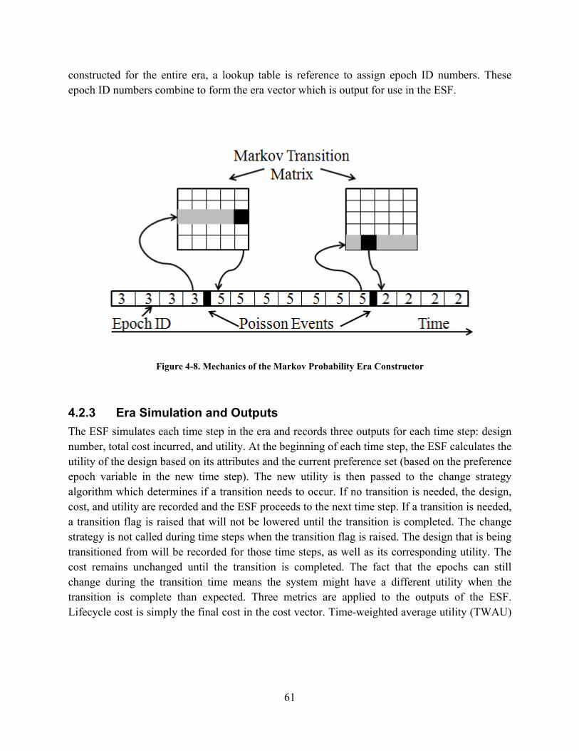
61

constructed for the entire era, a lookup table is reference to assign epoch ID numbers. These epoch ID numbers combine to form the era vector which is output for use in the ESF.

Figure 4-8. Mechanics of the Markov Probability Era Constructor

4.2.3 Era Simulation and Outputs

The ESF simulates each time step in the era and records three outputs for each time step: design number, total cost incurred, and utility. At the beginning of each time step, the ESF calculates the utility of the design based on its attributes and the current preference set (based on the preference epoch variable in the new time step). The new utility is then passed to the change strategy algorithm which determines if a transition needs to occur. If no transition is needed, the design, cost, and utility are recorded and the ESF proceeds to the next time step. If a transition is needed, a transition flag is raised that will not be lowered until the transition is completed. The change strategy is not called during time steps when the transition flag is raised. The design that is being transitioned from will be recorded for those time steps, as well as its corresponding utility. The cost remains unchanged until the transition is completed. The fact that the epochs can still change during the transition time means the system might have a different utility when the transition is complete than expected. Three metrics are applied to the outputs of the ESF. Lifecycle cost is simply the final cost in the cost vector. Time-weighted average utility (TWAU)

62

is used to measure the mean utility across the era7, even as the utility functions change. Time below threshold8 is the amount of time the utility was below some predetermined minimally acceptable value. Note that this threshold is not necessarily the same as the utility threshold in the change strategy.

4.3 Application to Space Tug The Space Tug data set contains designs for orbital transfer vehicles that can be used for a variety of on-orbit servicing missions such as observation of (potentially hostile) targets, assisting in orbit changes, and removing debris (McManus and Schuman 2003). This data set has been used for studies in changeability and survivability (Richards 2009, Ross and Hastings 2006). Recent work has added context variables to the existing preference curves used to define the epochs.

4.3.1 Epoch Variables

The Space Tug data set used for this study uses two epoch variables: mission and technology level (the only context variable). The missions are the preference sets and are composed of three single attribute vs. utility curves as well as weightings for the different attributes. The weighted sum of the single attribute utilities forms the multi-attribute utility, which for the purposes of this section is synonymous with “utility”. For this thesis, a mission describes a potential set of needs and can be thought of as requirements for a specific contract that the system’s performance will be evaluated against. The eight ”missions” considered in this simulation are: (1) baseline, (2) technology demonstration, (3) GEO rescue, (4) deployment assistance, (5) refueling and maintenance, (6) garbage collector, (7) all-purpose military, and (8) satellite saboteur. The transition matrix for preferences can be seen in Table 4-2.

7 While utility functions with different definitions cannot be aggregated, this statistic can be interpreted as “mean fraction of utopia utility satisfied.”

8 The “time above threshold” statistic is often used in survivability literature. Here, time below is used to reflect the fact that the emphasis is on avoiding long periods of dissatisfaction with performance.

63

Table 4-2. Hypothetical Markov Transition Matrix for Preference Sets (Space Tug "Missions")

Mission To 1 To 2 To 3 To 4 To 5 To 6 To 7 To 8 From 1 0.300 0.400 0.050 0.050 0.050 0.050 0.050 0.050 From 2 0.050 0.150 0.133 0.133 0.133 0.133 0.133 0.133 From 3 0.150 0.050 0.500 0.060 0.060 0.060 0.060 0.060 From 4 0.150 0.050 0.060 0.500 0.060 0.060 0.060 0.060 From 5 0.150 0.050 0.060 0.060 0.500 0.060 0.060 0.060 From 6 0.150 0.050 0.060 0.060 0.060 0.500 0.060 0.060 From 7 0.150 0.050 0.038 0.038 0.038 0.038 0.500 0.150 From 8 0.150 0.050 0.038 0.038 0.038 0.038 0.150 0.500

Each mission is composed of three single attribute utility curves (for the three attributes: manipulator mass, delta V, and response time) and corresponding weights. The single attribute utility curves for the three attributes are seen in Figure 4-9, Figure 4-10, and Figure 4-11, respectively. The SAU curves used for each mission set, along with the corresponding weights, are captured in Table 4-3.

Table 4-3. SAU Curves and Weights for Space Tug Missions

Mission Manipulator SAU Curve

Weight Response Time SAU Curve

Weight Delta V SAU Curve

Weight

1 A 0.30 A 0.10 A 0.60 2 B 0.70 A 0.10 A 0.20 3 A 0.20 B 0.20 B 0.60 4 C 0.60 A 0.30 C 0.10 5 D 0.75 A 0.05 D 0.20 6 E 0.20 A 0.05 E 0.75 7 A 0.40 A 0.20 F 0.40 8 F 0.20 B 0.20 A 0.60

64

Figure 4-9. Single Attribute Utility Curves for Manipulator Mass

Figure 4-10. Single Attribute Utility Curves for Response Time

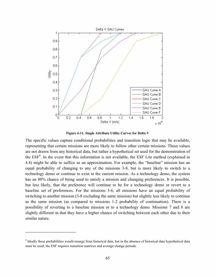
65

Figure 4-11. Single Attribute Utility Curves for Delta V

The specific values capture conditional probabilities and transition logic that may be available, representing that certain missions are more likely to follow other certain missions. These values are not drawn from any historical data, but rather a hypothetical set used for the demonstration of the ESF9. In the event that this information is not available, the ESF Lite method (explained in 4.4) might be able to suffice as an approximation. For example, the “baseline” mission has an equal probability of changing to any of the missions 3-8, but is more likely to switch to a technology demo or continue to exist in the current mission. As a technology demo, the system has an 80% chance of being used to satisfy a mission and changing preferences. It is possible, but less likely, that the preference will continue to be for a technology demo or revert to a baseline set of preferences. For the missions 3-6, all missions have an equal probability of switching to another mission (3-8 excluding the same mission) but slightly less likely to continue as the same mission (as compared to missions 1-2 probability of continuation). There is a possibility of reverting to a baseline mission or to a technology demo. Missions 7 and 8 are slightly different in that they have a higher chance of switching between each other due to their similar nature.

9 Ideally these probabilities would emerge from historical data, but in the absence of historical data hypothetical data must be used; the ESF requires transition matrices and average change periods.

66

Table 4-4. Markov Transition Matrix for Technology Level

Technology Level To 1 To 2 From 1 0 1 From 2 0 1

Technology is either “present level” or “future level” and affects the attribute levels associated with each design variable as well as the cost calculation. The attribute levels are then used to calculate utility. The context variable Markov transition matrix can be seen in Table 4-4. The future state is a sink; once the shift to “future level” technology occurs it cannot revert back to present technology.

4.3.2 Tradespace Definition

For Space Tug, the design variables originally introduced are manipulator size, propulsion system, and fuel mass (McManus and Schuman 2003). An additional variable, design for evolvability (DfE), was added for the purposes of this simulation. The DfE variable represents the inclusion of design heuristics that make redesign simpler and is treated as a mass penalty. The ranges of values for the design variables are seen in Table 4-5.

Table 4-5. Design Variable Levels (modified from McManus and Schuman 2003)

Design Variables Levels Manipulator Mass (kg) [300, 1000, 3000, 5000] Propulsion System Storable BiPropellant, Cryogenic, Electric, Nuclear Fuel Mass (kg) [30, 100, 300, 600, 1200, 3000, 10000, 30000] DfE (% Mass Penalty) [0, 20]

The three attributes calculated were capability, delta V, and response time. Capability is measured as the manipulator mass. Delta V is a function of all masses, specific impulse, and mass fraction. The latter two are properties of the propulsion system in use, as seen in Table 4-6. In cases where two values appear, the latter value is used in the future context. Response time is either fast or slow and is a function solely of the propulsion and is in the ‘Fast?’ column of Table 4-6.

Table 4-6. Propulsion System Values (McManus and Schuman 2003)

Propulsion System Isp (sec) Base Mass (kg) Mass Fraction Fast? Storable Bipropellant 300 0 0.12 Y Cryogenic 450/550 0 0.13 Y Electric 3000 25 0.25/0.3 N Nuclear 1500 1000/600 0.20 Y

The cost of a design is a function of its dry and wet mass. First, the propulsion system mass (Mp) must be calculated using base mass (mp0), mass fraction (mpf), and the fuel mass (Mf)

67

fpfpp MmmM 0

Next, the vehicle bus mass (Mb) is calculated using the propulsion system mass, manipulator mass (Mm), and bus mass fraction (mbf)

mbfpb MmMM

The bus mass fraction was held constant at 1 for this case study. The mass penalty for DfE is levied in the final mass calculations. The vehicle dry mass (Md) and vehicle wet mass (Mw) then are calculated as

fdw

mbd

MMM

MMDfEM

)1(

The dry mass cost (cd) of $150,000/kg and the wet mass cost (cw) of $15,000/kg in the present context ($10,000/kg in the future context) are used to then calculate total cost (C)10

ddww McMcC

Delta V is calculated as

d

wdsp M

MMIv ln

The baseline schedule for this simulation is a function of the propulsion system: bipropellant (8 months), cryogenic (9 months), electric (10 months), nuclear (12 months). The schedule is increased by 2 months if DfE is included in the design11. The schedule is the amount of time needed to design and build a given system. A representative tradespace showing how cost, utility, and schedule vary for different space tug designs is shown in Figure 4-12.

10 These cost values were adapted from McManus and Schuman (2003). The future context wet mass cost was proposed by Matt Fitzgerald.

11 The schedule values are hypothetical and were proposed in Fulcoly et al. (2012) to add a notional temporal aspect to the Space Tug tradespace.

68

Figure 4-12. Cost-Utility-Schedule Tradespace for All Designs Valid in Mission 8.

4.3.3 Change Mechanism

For Space Tug, the only epoch variable that affects transitions is technology level. The cost of transitioning is different in the future technology since some mass fractions and base masses change for the propulsion systems. For this study, the only change mechanism considered is “redesign with inheritance.” Redesign cost and schedule were calculated as a function of the similarity of the current and target designs.

To alter the clean-sheet cost of a design during redesign, a “reuse advantage” is applied. The reuse advantage lowers the cost of designing components that are already in use on the current design. Since cost is a function of mass in the Space Tug tradespace, reuse advantage is applied to mass. If a component, or design variable in the context of the Space Tug data set, is changed, the full component mass is used to calculate the cost. If a component does not change, its mass is reduced by the reuse advantage. If DfE is not included in the original design, the reuse advantage is zero. For this paper, if DfE is included, the reuse advantage is 50%. Identifying an appropriate reuse advantage is the subject of further research.

Redesign schedule (Sij) is a function of the new propulsion system, current DfE level (DfEi), and target DfE level (DfEj). The baseline schedule (Si) is the same as in the original design, based on

69

propulsion system. If the previous design included DfE, an evolvability advantage (EA) is subtracted from the schedule. [Note all DfE variables are binary for these equations12]

EPDfEEADfESS addediiij **

Where

ijadded DfEDfEDfE 1

EA = 3 months

EP = 2 months

In this simulation the evolvability advantage was 3 months, meaning the evolvable redesign process takes 3 months less time than that of a clean-sheet development of the same design. If DfE was not included in the original design but is to be included in the new design, the same 2 month evolvability penalty (EP) is applied. This penalty is not applied for continuing to have DfE (i.e., both the original and new design include DfE).

4.3.4 Results: Application of ESF

4.3.4.1 Experimental Setup

Each trial of the ESF is characterized by the change strategy it uses and any parameters used in that strategy (e.g., Strategy 3 using 5 year redesign cycles and 70th percentile utility threshold). The trial will loop through 1,000 eras, using each design (of the full factorial, 256 design tradespace from Table 4-5) as a starting design in each era. The change strategies are repeated in Table 4-7 for convenience.

Table 4-7. Inputs for Change Strategies

Strategy Name Inputs 1 Always Seek Highest Utility None 2 Exceed Utility Threshold Threshold Percentile 3 Exceed Utility Threshold at

Generation Intervals Threshold Percentile, Generation Length

12 The DfE variables are binary here for the purposes of the schedule equations only. Since the actual DfE percentage is used in the mass calculations, making the variable binary was not an option. These schedule equations are therefore only valid for the case of two DfE levels. As the number of DfE levels expands beyond two, schedule equations will need to be revisited.

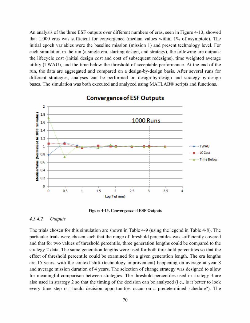
70

An analysis of the three ESF outputs over different numbers of eras, seen in Figure 4-13, showed that 1,000 eras was sufficient for convergence (median values within 1% of asymptote). The initial epoch variables were the baseline mission (mission 1) and present technology level. For each simulation in the run (a single era, starting design, and strategy), the following are outputs: the lifecycle cost (initial design cost and cost of subsequent redesigns), time weighted average utility (TWAU), and the time below the threshold of acceptable performance. At the end of the run, the data are aggregated and compared on a design-by-design basis. After several runs for different strategies, analyses can be performed on design-by-design and strategy-by-design bases. The simulation was both executed and analyzed using MATLAB® scripts and functions.

Figure 4-13. Convergence of ESF Outputs

4.3.4.2 Outputs

The trials chosen for this simulation are shown in Table 4-9 (using the legend in Table 4-8). The particular trials were chosen such that the range of threshold percentiles was sufficiently covered and that for two values of threshold percentile, three generation lengths could be compared to the strategy 2 data. The same generation lengths were used for both threshold percentiles so that the effect of threshold percentile could be examined for a given generation length. The era lengths are 15 years, with the context shift (technology improvement) happening on average at year 8 and average mission duration of 4 years. The selection of change strategy was designed to allow for meaningful comparison between strategies. The threshold percentiles used in strategy 3 are also used in strategy 2 so that the timing of the decision can be analyzed (i.e., is it better to look every time step or should decision opportunities occur on a predetermined schedule?). The

71

choice of redesign periods (2, 4, and 6 years) was based on matching the average mission duration (i.e. 4 years per mission) as well as being shorter and longer.

Table 4-8. Inputs for Change Strategies

Strategy Name Inputs 1 Always Seek Highest Utility None 2 Exceed Utility Threshold Threshold Percentile 3 Exceed Utility Threshold at

Generation Intervals Threshold Percentile, Generation Length

Table 4-9. Description of Trials

Trial Strategy (see Table 4-8) Threshold Percentile Redesign Period (Years) 1 1 - - 2 2 20 - 3 2 40 - 4 2 60 - 5 2 80 - 6 3 40 2 7 3 40 4 8 3 40 6 9 3 80 2 10 3 80 4 11 3 80 6

The results of the 11 trials described in Table 4-9 are listed in Table 4-10. The figures given represent the aggregates over all 256 designs and 1000 eras, the highest/lowest average for a design across the 1000 eras, and the corresponding design. Strategy 3 had the lowest average lifecycle cost ($1.73B), followed by strategy 2 ($1.89B) and strategy 1 ($3.50B). In the strategy 2 trials, average lifecycle cost went down as the threshold percentile decreased. In strategy 3, the cost decreased as the generation length increased. For trials with the same generation length, the trial with the lowest threshold percentile always had a lower lifecycle cost, which is in agreement with the inverse correlation between lifecycle cost and threshold percentile seen in the strategy 2 trials.

The strategy with the lowest average time below acceptability was strategy 1 (13.8 months), followed by strategy 2 (31.2 months) and strategy 3 (38.5 months). In strategy 2, average time below acceptability decreased as the threshold percentile increased. This trend was also seen in the strategy 3 trials with generation length held constant. In strategy 3, the average time below acceptability increased as generation length increased.

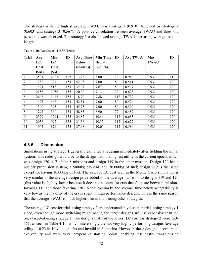
72

The strategy with the highest average TWAU was strategy 1 (0.910), followed by strategy 2 (0.603) and strategy 3 (0.567). A positive correlation between average TWAU and threshold percentile was observed. The strategy 3 trials showed average TWAU increasing with generation length.

Table 4-10. Results of 11 ESF Trials

Trial Avg LC Cost ($M)

Min LC Cost ($M)

ID Avg Time Below (months)

Min Time Below (months)

ID Avg TWAU Max TWAU

ID

1 3501 2403 145 13.76 8.00 72 0.910 0.937 112 2 1282 324 154 52.08 9.00 80 0.511 0.931 120 3 1491 518 154 34.07 9.67 80 0.547 0.931 120 4 2158 1056 155 20.60 9.13 72 0.623 0.931 120 5 2646 1442 153 18.20 9.88 112 0.732 0.931 120 6 1423 466 154 42.81 9.00 80 0.524 0.931 120 7 1340 395 154 45.23 9.00 80 0.500 0.931 120 8 1297 360 154 48.83 8.90 72 0.482 0.931 120 9 2379 1244 153 24.82 10.44 112 0.683 0.931 120 10 2056 992 153 31.56 10.33 112 0.627 0.931 120 11 1902 874 153 37.68 10.01 112 0.584 0.931 120

4.3.5 Discussion

Simulations using strategy 1 generally exhibited a redesign immediately after fielding the initial system. This redesign would be to the design with the highest utility in the current epoch, which was design 120 in 7 of the 8 missions and design 119 in the other mission. Design 120 has a nuclear propulsion system, a 5000kg payload, and 30,000kg of fuel; design 119 is the same except for having 10,000kg of fuel. The average LC cost seen in the Monte Carlo simulation is very similar to the average design price added to the average transition to designs 119 and 120 (this value is slightly lower because it does not account for eras that fluctuate between missions favoring 119 and those favoring 120). Not surprisingly, the average time below acceptability is very low as the majority of the era is spent in high performance designs. This is the same reason that the average TWAU is much higher than in trials using other strategies.

The average LC cost for trials using strategy 2 are understandably less than trials using strategy 1 since, even though more switching might occur, the target designs are less expensive than the ones targeted using strategy 1. The designs that had the lowest LC cost for strategy 2 were 153-155, as seen in Table 4-10, which interestingly are not very highly performing designs (average utility of 0.23 in 10 valid epochs and invalid in 6 epochs). However, these designs incorporated evolvability and were very inexpensive starting points, enabling less costly transitions to

73

appropriate designs. The cost increases as threshold percentile increases since there are more situations where the change decision is triggered. The time below acceptability increased as threshold percentile decreased because the utility of the designs in use were more likely to be close to (just above) the threshold percentiles. The data showed a positive correlation between TWAU and threshold percentile for strategy 2.

Table 4-11. Designs of Interest

Design # DfE Prop Type Fuel Mass (kg) Manipulator Mass (kg)

Category of High Performance

72 0 BiProp 30000 3000 Time Below 80 0 Cryo 30000 3000 Time Below 112 0 Cryo 30000 5000 Time Below, TWAU 120 0 Nuclear 30000 5000 TWAU 145 1 Nuclear 30 300 LC Cost 153 1 Electric 30 300 LC Cost 154 1 Electric 100 300 LC Cost 155 1 Electric 300 300 LC Cost

The average LC cost decreases as generation length increases in strategy 3 because there are fewer opportunities for change costs to be incurred. As in strategy 2, designs 153-155 dominate the lowest LC cost category. The average time below acceptability decreases as generation length increases since it is related to the time between becoming unacceptable and triggering change, which is a function (among other variables) of generations length. Designs 72, 80, and 112, seen in Table 4-11, were the best performers in the time below acceptability criterion for all three strategies. This is due to the fact that they are high performing designs with short schedules; none of them incur a DfE penalty and use the propulsion systems that take the least amount time to build. In the set of trials using a threshold percentile of 40, there was approximately 5% decrease in TWAU with each 2 years of generation length added. In the trials using 80 as a threshold there was approximately 5% decrease in TWAU with each 2 years of generation length added. Design 120, seen in Table 4-11, tended to dominate the TWAU column due to having the best performance in 7 of the 8 missions.

In general, there was not an obvious choice for generation length that emerged. Figure 4-14 and Figure 4-15 show how increasing generation length has positive cost implications and negative utility implications, whereas decreasing generation length has opposite effects. A tradeoff between the two effects, influenced by the stakeholder’s relative concerns about cost and utility, will lead to the “sweet spot” for a given scenario. The inclusion of DfE was beneficial for designs that did not have a high or acceptable utility in a majority of different epochs since they often needed to go through multiple transitions. In the event that a design has very high utility in all or most epochs, DfE can be safely excluded since the chance of needing to make a transition is low.

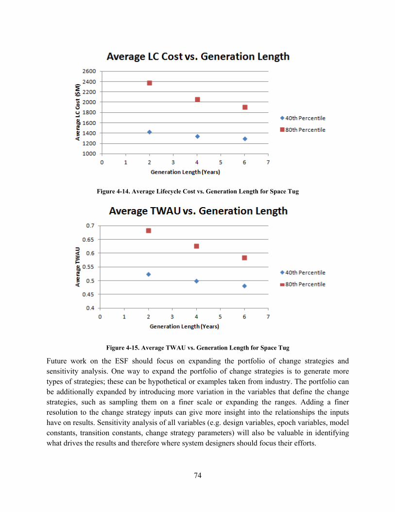
74

Figure 4-14. Average Lifecycle Cost vs. Generation Length for Space Tug

Figure 4-15. Average TWAU vs. Generation Length for Space Tug

Future work on the ESF should focus on expanding the portfolio of change strategies and sensitivity analysis. One way to expand the portfolio of change strategies is to generate more types of strategies; these can be hypothetical or examples taken from industry. The portfolio can be additionally expanded by introducing more variation in the variables that define the change strategies, such as sampling them on a finer scale or expanding the ranges. Adding a finer resolution to the change strategy inputs can give more insight into the relationships the inputs have on results. Sensitivity analysis of all variables (e.g. design variables, epoch variables, model constants, transition constants, change strategy parameters) will also be valuable in identifying what drives the results and therefore where system designers should focus their efforts.

75

4.4 ESF Lite

The ESF requires a significant amount of information about the uncertainty in epoch variables before it can be implemented. A “back of the envelope” method, heretofore referred to as ESF Lite, for applying the concepts of the ESF has been hypothesized, but not tested. This method only answers the question of “what should the generation length be for this architecture?”, but does not require as much information about the epoch variables (e.g. transition matrices). A matrix is generated with the epoch variables on one dimension and system components on the other dimension. A zero or one is placed in each cell. An entry of one corresponds to “this component would potentially need to change to maintain attribute levels given a significant change in this epoch variable.” “Significant” is defined by the stakeholders (e.g. 10% change in value). The sum of the cells is calculated for each epoch variable, and the average change period (defined as the average amount of time between “significant” changes) for the epoch variable with the highest sum should be the generation length. A demonstrative example of how the ESF Lite would be applied is shown below and in Table 4-12.

System X has 5 components (design variables) that will be denoted as C.1 through C.5. There are 4 epoch variables that can potentially change during an era, denoted as E.1 through E.4.

Table 4-12. Example Application of ESF Lite

Design Variables Row Sum

Average Change Period C.1 C.2 C.3 C.4 C.5

Epo

ch

Var

iabl

es E.1 1 1 0 0 1 3 4 years

E.2 0 0 1 0 0 1 1 year E.3 1 0 0 1 0 2 2 years E.4 0 1 0 0 0 1 1 year

Epoch variable E.1 is identified as having the highest sum. Accordingly, system X should have a generation length of 4 years to best syncopate with changes in its environment. The ESF Lite method has not yet been formally applied or tested and should be the topic of future research. Possible modifications to the ESF light include: differentiating between architecture and non-architecture variables, using weighted values rather than binary values in the matrix to show strength of relationship, and taking cost into account.

76

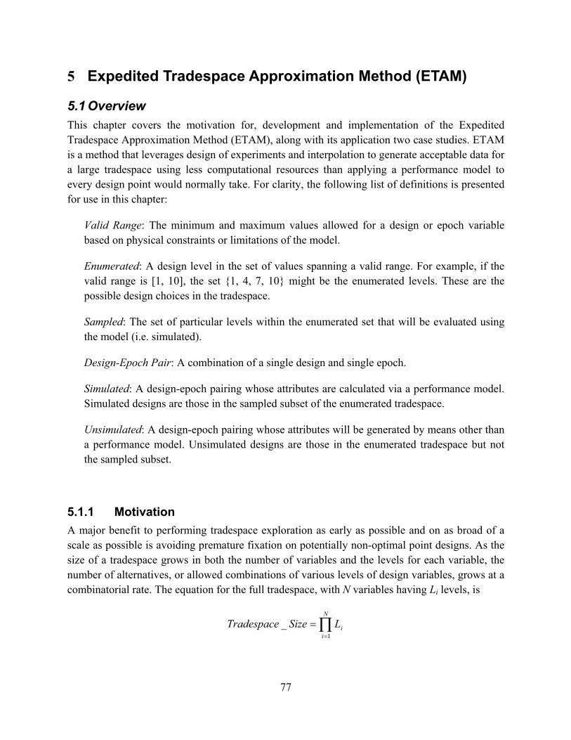
77

5 Expedited Tradespace Approximation Method (ETAM)

5.1 Overview This chapter covers the motivation for, development and implementation of the Expedited Tradespace Approximation Method (ETAM), along with its application two case studies. ETAM is a method that leverages design of experiments and interpolation to generate acceptable data for a large tradespace using less computational resources than applying a performance model to every design point would normally take. For clarity, the following list of definitions is presented for use in this chapter:

Valid Range: The minimum and maximum values allowed for a design or epoch variable based on physical constraints or limitations of the model.

Enumerated: A design level in the set of values spanning a valid range. For example, if the valid range is [1, 10], the set {1, 4, 7, 10} might be the enumerated levels. These are the possible design choices in the tradespace.

Sampled: The set of particular levels within the enumerated set that will be evaluated using the model (i.e. simulated).

Design-Epoch Pair: A combination of a single design and single epoch.

Simulated: A design-epoch pairing whose attributes are calculated via a performance model. Simulated designs are those in the sampled subset of the enumerated tradespace.

Unsimulated: A design-epoch pairing whose attributes will be generated by means other than a performance model. Unsimulated designs are those in the enumerated tradespace but not the sampled subset.

5.1.1 Motivation

A major benefit to performing tradespace exploration as early as possible and on as broad of a scale as possible is avoiding premature fixation on potentially non-optimal point designs. As the size of a tradespace grows in both the number of variables and the levels for each variable, the number of alternatives, or allowed combinations of various levels of design variables, grows at a combinatorial rate. The equation for the full tradespace, with N variables having Li levels, is

N

iiLSizeTradespace

1

_

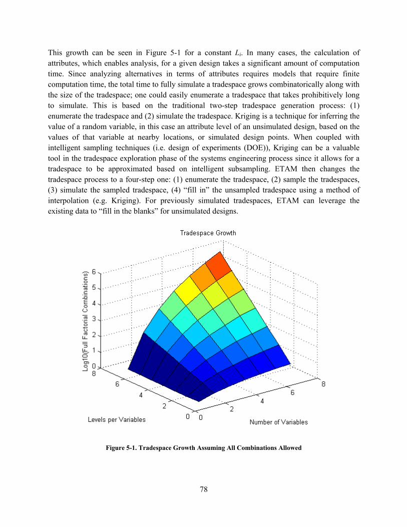
78

This growth can be seen in Figure 5-1 for a constant Li. In many cases, the calculation of attributes, which enables analysis, for a given design takes a significant amount of computation time. Since analyzing alternatives in terms of attributes requires models that require finite computation time, the total time to fully simulate a tradespace grows combinatorically along with the size of the tradespace; one could easily enumerate a tradespace that takes prohibitively long to simulate. This is based on the traditional two-step tradespace generation process: (1) enumerate the tradespace and (2) simulate the tradespace. Kriging is a technique for inferring the value of a random variable, in this case an attribute level of an unsimulated design, based on the values of that variable at nearby locations, or simulated design points. When coupled with intelligent sampling techniques (i.e. design of experiments (DOE)), Kriging can be a valuable tool in the tradespace exploration phase of the systems engineering process since it allows for a tradespace to be approximated based on intelligent subsampling. ETAM then changes the tradespace process to a four-step one: (1) enumerate the tradespace, (2) sample the tradespaces, (3) simulate the sampled tradespace, (4) “fill in” the unsampled tradespace using a method of interpolation (e.g. Kriging). For previously simulated tradespaces, ETAM can leverage the existing data to “fill in the blanks” for unsimulated designs.

Figure 5-1. Tradespace Growth Assuming All Combinations Allowed

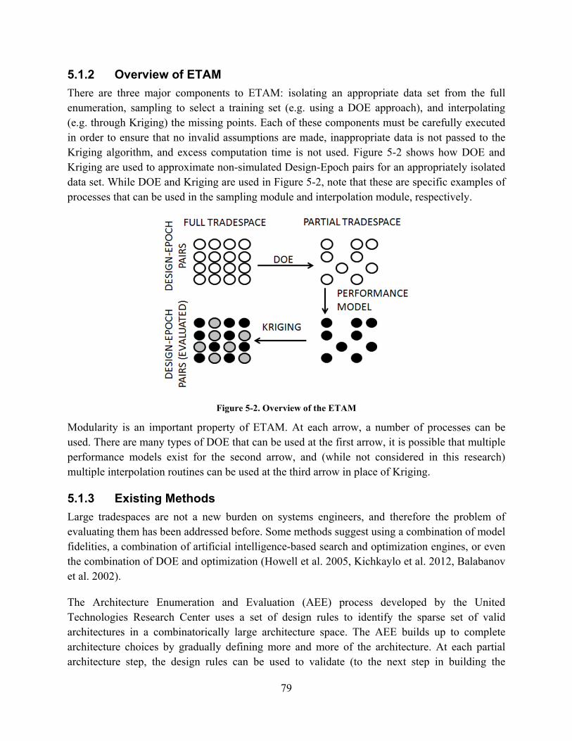
79

5.1.2 Overview of ETAM

There are three major components to ETAM: isolating an appropriate data set from the full enumeration, sampling to select a training set (e.g. using a DOE approach), and interpolating (e.g. through Kriging) the missing points. Each of these components must be carefully executed in order to ensure that no invalid assumptions are made, inappropriate data is not passed to the Kriging algorithm, and excess computation time is not used. Figure 5-2 shows how DOE and Kriging are used to approximate non-simulated Design-Epoch pairs for an appropriately isolated data set. While DOE and Kriging are used in Figure 5-2, note that these are specific examples of processes that can be used in the sampling module and interpolation module, respectively.

Figure 5-2. Overview of the ETAM

Modularity is an important property of ETAM. At each arrow, a number of processes can be used. There are many types of DOE that can be used at the first arrow, it is possible that multiple performance models exist for the second arrow, and (while not considered in this research) multiple interpolation routines can be used at the third arrow in place of Kriging.

5.1.3 Existing Methods

Large tradespaces are not a new burden on systems engineers, and therefore the problem of evaluating them has been addressed before. Some methods suggest using a combination of model fidelities, a combination of artificial intelligence-based search and optimization engines, or even the combination of DOE and optimization (Howell et al. 2005, Kichkaylo et al. 2012, Balabanov et al. 2002).

The Architecture Enumeration and Evaluation (AEE) process developed by the United Technologies Research Center uses a set of design rules to identify the sparse set of valid architectures in a combinatorically large architecture space. The AEE builds up to complete architecture choices by gradually defining more and more of the architecture. At each partial architecture step, the design rules can be used to validate (to the next step in building the

80

architecture) or eliminate an entire subtree of architectures. This process ensures that each architecture is considered while not actually having to physically evaluate every architecture in the search for all feasible choices (Murray et al. 2011). This method is very effective when design rules are known a priori, but ETAM serves to populate a set of designs separate from any value statement. ETAM and AEE could work effectively together, with AEE filtering which designs are valid and handing the valid designs over to ETAM for evaluation.

The method proposed in (Howell et al. 2005) calls for the use of a lower fidelity model to examine a full-factorial tradespace and then use of a higher fidelity model to evaluate areas of interest identified by the first model. The authors propose that their method is a “versatile modeling framework which (1) allows a rapid assessment of the broader architectural tradespace, (2) evaluates high-level metrics for comparing competing architectures, (3) models “second-order” couplings between design parameters, and (4) identifies favorable classes of architectures.” While this method has value when multiple models of varying fidelity are available, ETAM seeks to save computational time in the presence of a single model.

The System Platform for Integrated Design in Real-Time (SPIDR) analyzes large tradespaces by combining artificial intelligence-based search and an optimization engine (Kichkaylo et al. 2012). SPIDR is a “constraint-based design synthesis engine” that does not require a utility function or collapsing multiple performance dimensions. For a set of design variables, architecture rules, mission requirements, and optimization metrics, SPIDR returns a “best” design. A single answer such as a “best” design is not always as valuable as having a tradespace to explore in search of many answers. ETAM, unlike SPIDR, does not seek to provide a solution, only to populate a tradespace with approximated attribute values. SPIDR combines exploration and optimization, whereas ETAM serves only to aid in exploration.

The Applied Research Laboratory (ARL) at Penn State developed a method called the ARL tradespace visualizer (ATSV) that provides a multitude of tools for visualizing, navigating, and evaluating complex tradespaces. One of the tools in ATSV involves choosing an “attractor” in the tradespace to simulate new designs “nearby.” The ATSV engine uses a differential evolution (DE) algorithm and a response surface model (when quicker than querying the full model) to populate points near the attractor with improving fitness (Normalized Euclidian distance from the attractor). Alternatively, the attractor can be replaced with a preference function to use with DE to find points of increasing preference (Stump et al. 2009). The ATSV provides value in a different way than ETAM, specifically in that it combines fitness with the tradespace population problem. ETAM does not seek to include a fitness function. Much of ASTV’s value is derived from its excellent visualization ability, a function that ETAM does not include.

VisualDOC is a commercially available tool that, similar to SPIDR, couples exploration, analysis, and optimization (Balabanov et al. 2002). Another focus of VisualDOC is a user

81

interface that allows a user without knowledge of DOE or optimization to still leverage those concepts when exploring a tradespace.

Figure 5-3. General VisualDOC Structure (Balabanov et al. 2002)

The high-level model of VisualDOC can be seen in Figure 5-3. An aspect of VisualDOC that ETAM hopes to emulate is the high degree of modularity13. VisalDOC’s modularity could potentially lead to a specific instance of it representing ETAM, but at this time Kriging is not one of the interpolation models available. A long-term goal for ETAM is to have “plug’n’play” modularity with respect to the type of DOE used and the type of interpolation.

Exploring these existing methods reveals that there are many valuable methods for aiding tradespace exploration already in use. This does not mean that ETAM was created in vain; ETAM still plays a unique role. Unlike many of the methods explored, ETAM decouples the processes of tradespace generation and tradespace exploration. Methods like VisualDOC, ATSV, and SPIDR are built around the idea of optimization; the “best” design is often an output. On the other hand, ETAM is a front end to exploration that creates data that might not have been otherwise available, leaving the specific method of analysis up to the analyst.

5.2 Implementation ETAM can be described as a process with 3 steps:

1. Partition the enumerated design-epoch tradespace into appropriate sets for interpolation 2. Select an appropriate training set for each of the isolated data sets 3. Interpolate the remainder of the isolated data sets

13 While in theory VisualDOC could adopt Kriging as one of its methods, at this time the documentation does not list it as a method in use.

82

The Satellite Radar case study is be used to help illustrate the first two steps for clarity. The Satellite Radar case study contains 8 design variables and 6 epoch variables that specify a constellation of ground-observing radar satellites.

5.2.1 Partitioning the enumerated tradespace

The dependent variables of interest in tradespace exploration are attributes and cost. These attributes are a function of design variables and epoch variables, the independent variables of tradespace exploration. Variables come in several types: ratio, ordinal, interval, and nominal. These types, seen in Table 5-1, are classified as either Krigable or Non-Krigable depending on whether or not an interpolation scheme such as Kriging can be used to approximate attributes for differing levels of a variable of that type. Since the difference between independent variables is considered in Kriging, only interval and ratio variables are considered Krigable.

Table 5-1. Variable Types (Siegel 1957)

Variable Type

Explanation Example Classification

Ratio The difference between two values is meaningful and there is a definition of zero.

Temperature (K or R), Power, Length, Time

Krigable

Interval The difference between two values is meaningful.

Temperature (F or C), Krigable

Ordinal Order matters but not the difference between values.

Technology Readiness Level (TRL)

Non-Krigable

Nominal Mutually exclusive, but not necessarily ordered (i.e. categorical).

Binary Variables (On/Off), ID #s

Non-Krigable

The first step of ETAM, accordingly, is to segregate the design and epoch variables into Krigable and non-Krigable variables. This has been done for the Satellite Radar tradespace in Table 5-2. While all the epoch variables in this case happen to be non-Krigable, it is important to note that this will not always be the case. Any variables that are not inputs to the performance model should not be considered in ETAM, regardless of the variable type. Including such variables as non-Krigable will unnecessarily increase computation time. Including such variables as Krigable will pass non-unique points to the Kriging routine, detracting from the quality of the fit.

83

Table 5-2. Design Variable List for Satellite Radar (Krigable variables are italicized)

Design Variable Scale Type

Valid Range Enumerated Levels # Levels

Altitude Ratio 800 – 1500 [km] 800, 1200, 1500 [km] 3

Constellation Configuration Nominal 1 – 8 [int] 8 walker IDs 8

Antenna Area Ratio 10 – 100 [m2] 10, 40, 100 [m2] 3

Peak Transmit Power Ratio 1.5 – 20 [kW] 1.5, 10, 20 [kW] 3

Radar Bandwidth Ratio 0.5 – 2 [GHz] 0.5, 1, 2 [GHz] 3

Communication Downlink Nominal Relay or Direct Downlink

Relay, Direct Downlink

2

Tactical Communication Nominal Able or Not Able Able, Not Able 2

Maneuver Capability Ordinal 1 – 4 [x base fuel] 1x, 2x, 4x Base Fuel 3

Table 5-3. Epoch Variable List for Satellite Radar (Krigable variables are italicized)

Epoch Variable Scale Type

Valid Range Enumerated Levels # Levels

Available Radar Technology Ordinal 9 – 3 [TRL] Mature, Medium, Advanced

3

Communications Infrastructure

Nominal 0 – 2 [int] AFSCN, WGS + AFSCN, Third

3

Target Set Nominal 1 – 60 [int] Lookup Table of 9 Regions and Ops Plans

9

Collaborative AISR Assets Nominal Available or Not Available

Available, Not Available

2

Threat Environment Nominal No Jamming or Hostile Jamming

No Jamming, Hostile Jamming

2

Mission Priorities Nominal SAR <GMTI, SAR=GMTI, SAR<GMTI

SAR < GMTI, SAR = GMTI, SAR < GMTI

3

Once the variable space has been appropriately segregated, statistics about how many times the Kriging routine (second and third steps of ETAM) will be run can be calculated. For each

84

attribute, the Kriging routine will need to be run for each combination of non-Krigable variables. For Satellite Radar, this is the product of the number of levels for all the non-Krigable epoch variables and design variables: 93,312 (1.2% of the full factorial design-epoch space). Taking into account that there are 12 attributes in the case study, this means the interpolation routine will actually be run 1,119,744 times.

5.2.2 Selecting the training set (using DOE)

Once an appropriate data set (heretofore referred to as the Krigable subset) has been isolated for Kriging, the data set must be partitioned into a training set and Kriging set. The training set is the set of points whose attributes will be fully simulated and used to create the Kriging matrix, the matrix that is used in the interpolation of unsimulated points. The Kriging set is the set difference between the Krigable subset and the training set. The design and epoch variables of each point in the Kriging set will be used in conjunction with the Kriging matrix to interpolate the corresponding attributes. Using DOE to differentiate between the training set and the Kriging set allows for the intelligent sampling of the Krigable subset.

Remembering the way the Krigable subset was selected, we know that all designs in the set have the same levels for all non-Krigable variables (thus varying only along the Krigable variables). Assuming there are N Krigable variables each having Ln levels, the size of the Krigable subset will be

N

iiLS

1

The Krigable subset S will be partitioned into a training set, T, and a Kriging set, K. Only the T (<S) points in the training set, selected by DOE, will need to be simulated, leaving K = S – T points to be interpolated by the Kriging routine. The particular method of DOE will determine which points in S will be in T. The method of DOE used for Satellite Radar was a Box-Benkhen experimental design (Box & Benkhen 1960)14. Box-Benkhen designs use three levels for each factor. If a Krigable variable has an odd number of levels, the end points and center point of that factor are the three levels. If a Krigable variable has an even number of levels there are three options: (1) create an additional point in the design space, (2) treat it as a non-Krigable variable, or (3) use a different type of DOE. Furthermore, a Box-Benkhen design is only valid for >2 factors. Table 5-4 shows the savings for different numbers of Krigable variables. For simplicity in calculating S, T, and K, Table 5-4 considers all Krigable variables to have only three levels.

14 Box-Benkhen designs are not the only experimental designs that can be used. The Box-Benkhen design was applicable for Satellite Radar because of its 3-level nature. Other designs, such as D-optimal designs, can be used in more general cases.

85

Table 5-4. Box-Benkhen Savings for Three-Level Variables

# Krigable Variables (i) Points in S (Si) Points in T (Ti) Points in K (Ki) Savings (K/S) 3 27 13 14 52% 4 81 25 56 69% 5 243 41 202 83% 6 729 49 680 93% 7 2187 57 2130 97%

Depending on how much the designer knows about the model and the relationships between Krigable variables and attributes, further savings might be possible. If a Krigable variable has no impact on an attribute the Kriging routine will receive 2 identical attribute values, one for each value of the non-impacting Krigable variable, for each combination of Krigable variables (excluding the non-impacting variable). These identical points are bad for two reasons: (1) it worsens the accuracy of the Kriging interpolation while (2) increasing the computation time on the order of (Ti – Ti-1)

2. For this reason, it is beneficial to make a binary domain mapping matrix (DMM) (Danilovic & Browning 2007) that identifies which Krigable variables affect which attributes. The binary DMM for Satellite Radar is shown in Table 5-5. Interestingly enough, none of the 12 attributes are a function of all four Krigable variables15. An example of an attribute that is a function only of one variable is shown in Figure 5-4 and one that is a function of three variables is shown in Figure 5-5.

15 It is important to note that the only design variables being considered here are the Krigable variables. Any of the 12 attributes might additionally be a function of the non-Krigable variables.

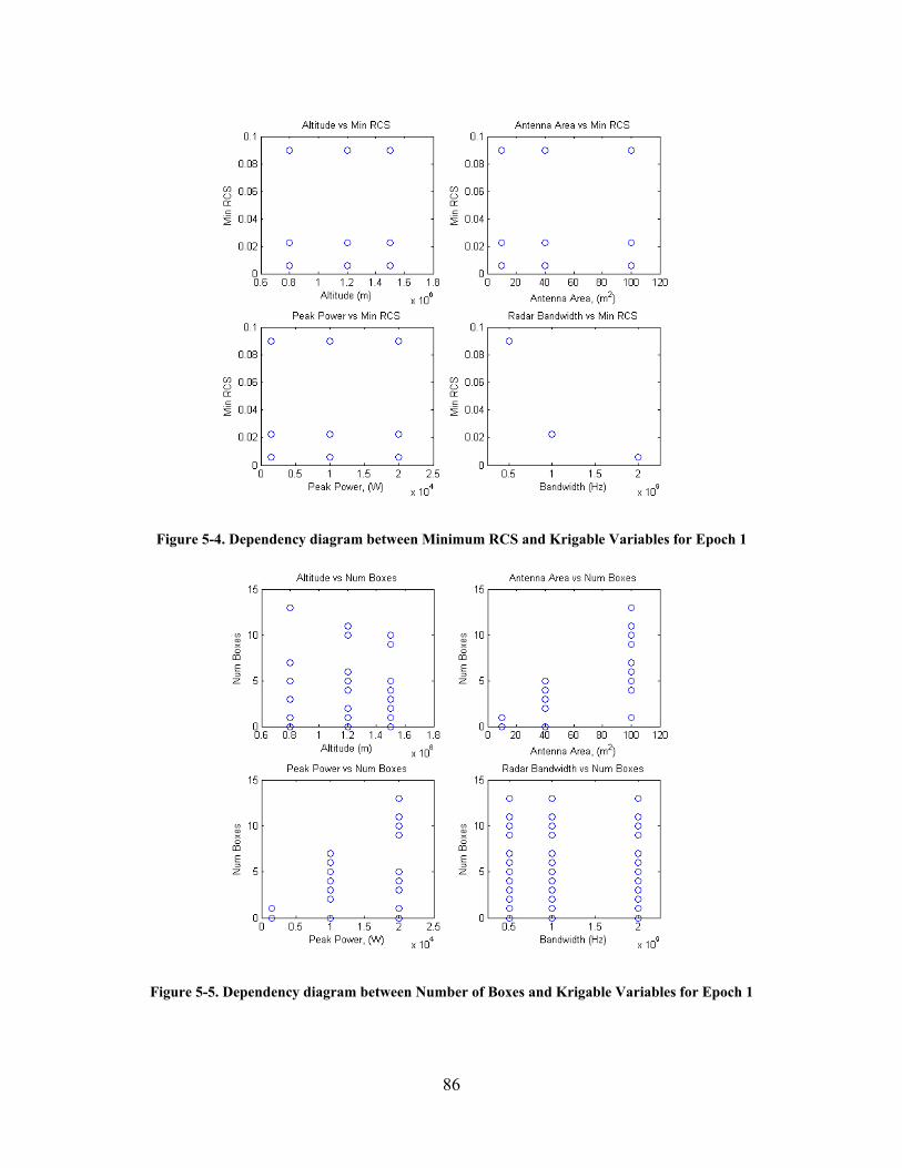
86

Figure 5-4. Dependency diagram between Minimum RCS and Krigable Variables for Epoch 1

Figure 5-5. Dependency diagram between Number of Boxes and Krigable Variables for Epoch 1

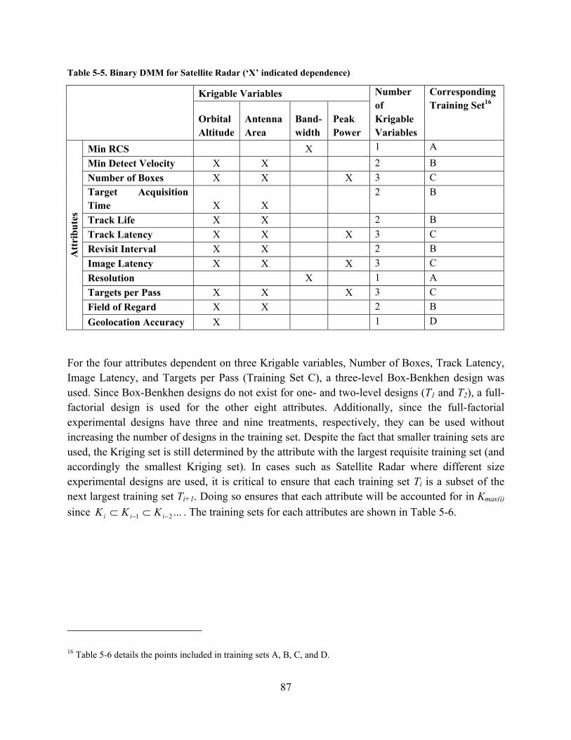
87

Table 5-5. Binary DMM for Satellite Radar (‘X’ indicated dependence)

Krigable Variables Number of Krigable Variables

Corresponding Training Set16

Orbital Altitude

Antenna Area

Band-width

Peak Power

Att

rib

ute

s

Min RCS X 1 A

Min Detect Velocity X X 2 B

Number of Boxes X X X 3 C

Target Acquisition Time X X

2 B

Track Life X X 2 B

Track Latency X X X 3 C

Revisit Interval X X 2 B

Image Latency X X X 3 C

Resolution X 1 A

Targets per Pass X X X 3 C

Field of Regard X X 2 B

Geolocation Accuracy X 1 D

For the four attributes dependent on three Krigable variables, Number of Boxes, Track Latency, Image Latency, and Targets per Pass (Training Set C), a three-level Box-Benkhen design was used. Since Box-Benkhen designs do not exist for one- and two-level designs (T1 and T2), a full-factorial design is used for the other eight attributes. Additionally, since the full-factorial experimental designs have three and nine treatments, respectively, they can be used without increasing the number of designs in the training set. Despite the fact that smaller training sets are used, the Kriging set is still determined by the attribute with the largest requisite training set (and accordingly the smallest Kriging set). In cases such as Satellite Radar where different size experimental designs are used, it is critical to ensure that each training set Ti is a subset of the next largest training set Ti+1. Doing so ensures that each attribute will be accounted for in Kmax(i)

since ...21 iii KKK . The training sets for each attributes are shown in Table 5-6.

16 Table 5-6 details the points included in training sets A, B, C, and D.

88

Table 5-6. Training Sets for Satellite Radar

Point ID

Krigable Variable Level Index (1, 2, or 3) Training Set Membership (from Table 5-5)

Orbital Altitude

Antenna Area

Bandwidth Peak Power

A (T1) B (T2) C (T3) D (T1)

1 1 1 1 2 X X X X

2 1 3 1 2 X X

3 3 1 3 2 X X X X

4 3 3 1 2 X X

5 1 2 1 1 X X

6 1 2 1 3 X

7 3 2 1 1 X X

8 3 2 1 3 X

9 2 1 2 1 X X X X

10 2 1 1 3 X

11 2 3 1 1 X

12 2 3 1 3 X X

13 2 2 1 2 X X

As seen in Table 5-6, training set C is T3, training set B is T2, and both training sets A and D are T1. Note that training set A only needed to contain one point with each level for bandwidth and training set D only needed to contain one point with each level for orbital altitude. Since the attributes these training sets are being used for are a function of only one of the Krigable variables, it is not necessary to hold the other Krigable variables constant. A single three point

set was sufficient for satisfying both training sets A and D. The table clearly shows 321 TTT .

The Kriging set then is K3, or all designs (of a 4-factor, 3-level full factorial design) not seen in Table 5-6.

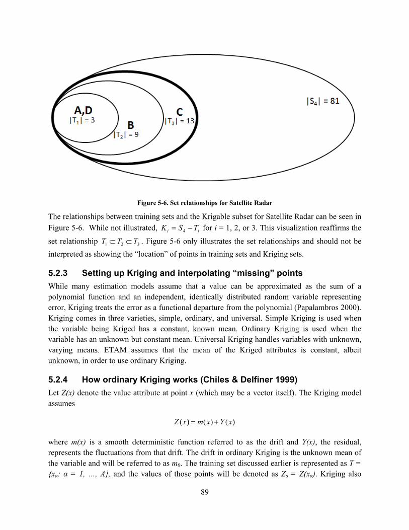
89

Figure 5-6. Set relationships for Satellite Radar

The relationships between training sets and the Krigable subset for Satellite Radar can be seen in

Figure 5-6. While not illustrated, ii TSK 4 for i = 1, 2, or 3. This visualization reaffirms the

set relationship 321 TTT . Figure 5-6 only illustrates the set relationships and should not be

interpreted as showing the “location” of points in training sets and Kriging sets.

5.2.3 Setting up Kriging and interpolating “missing” points

While many estimation models assume that a value can be approximated as the sum of a polynomial function and an independent, identically distributed random variable representing error, Kriging treats the error as a functional departure from the polynomial (Papalambros 2000). Kriging comes in three varieties, simple, ordinary, and universal. Simple Kriging is used when the variable being Kriged has a constant, known mean. Ordinary Kriging is used when the variable has an unknown but constant mean. Universal Kriging handles variables with unknown, varying means. ETAM assumes that the mean of the Kriged attributes is constant, albeit unknown, in order to use ordinary Kriging.

5.2.4 How ordinary Kriging works (Chiles & Delfiner 1999)

Let Z(x) denote the value attribute at point x (which may be a vector itself). The Kriging model assumes

)()()( xYxmxZ

where m(x) is a smooth deterministic function referred to as the drift and Y(x), the residual, represents the fluctuations from that drift. The drift in ordinary Kriging is the unknown mean of the variable and will be referred to as m0. The training set discussed earlier is represented as T = {xα: α = 1, …, A}, and the values of those points will be denoted as Zα = Z(xα). Kriging also

90

requires a measure of spatial dependence, or variogram, between the points in the training set and the points to be interpolated. The use of the variogram represents treating the drift as systematic (based on location), rather than random, as Y(x) was. The variogram evaluated for any two points xα and xβ will be denoted as σαβ = σ (xα, xβ). The point being estimated will be referred to as x0 and its estimated value Z* takes the form

A

xxZxxZ1

0000 )()()()(*

or, in its shorter form:

0* ZZ

Each λα represents a weight that is a function of the location x0 and λ0 is a constant based on x0. These weights are what Kriging seeks to find. The goal is find an estimate for Z* that minimizes the mean squared error (MSE):

2002

0 )*()*()*( ZZEZZVarZZE

The bias (rightmost term of the above equation) can be expanded using the expression for Z* and the mean m0 to obtain

00

0000

1

)*(

m

mmZZE

Setting Equation 5 equal to zero leaves us with the condition

00 1 m

Without knowledge of m0, the only guaranteed solution is when λ0 = 0, leaving us with the condition:

1

This is the first of the conditions that needs to be met. The remaining degrees of freedom (λα) are handled my minimizing the variance, which can be expanded to:

91

0000 2)*(

ZZVar

The variance can be minimized by choosing the λ that set the partial derivative of the variance with respect to λα equal to zero:

0

0

00

2

20

2)*(

ZZVar

We are now left with A +1 equations and can solve for the A remaining weights (λα and λ0 = 0 from the earlier assumption).

1

,...,12 0

A

Keep in mind that the variogram between each point xα in the training set and the point to be interpolated (x0) is represented as σα0 while the variogram between two points xα and xβ is σαβ.

5.2.5 Computational implementation (Press et al. 2007)

The first step in the computational implementation of Kriging is to prepare the 1 x Ti vector of simulated attribute values (ZT) in a training set as well as the i x Ti matrix of Krigable variable values (XT). The value i is the number of Krigable variables that affect the attribute being Kriged. A default β value of 1.5 was used based on a recommendation in Press et al. (2007). The Kriging routine takes in ZT, XT, β, and an indicator that signals whether or not a logarithmic transform will be used. The first step in the routine is to take the base-10 logarithm of the values in ZT if the variable is flagged for the transform. Next, the function linearly maps the values in ZT to [0, 1] for simplicity. This new matrix will be referred to as ZT0 and is calculated as:

)min()max(

)min(0

TT

TTT ZZ

ZZZ

The same process is used to transform XT into XT0. Next, the variogram is calculated. The variogram used in this implementation is a power law model because of its ability to generate good results while remaining computationally simple (Chiles & Delfiner 1999, Press et al. 2007)

rrv )(

92

Notice that the residual (the object of Kriging) is a stationary random process, hence the variogram is a function only of r = ||xj - xk|| and not explicitly of any input x value. Since ordinary Kriging assumes the attribute has a constant mean, the variogram satisfies the following condition:

2

)()()(2 kj xyxyErv

Since β and the x values in the training set have been specified, the routine must only calculate α (note that this is not the same α used in the derivation of Kriging) such that the variogram satisfies the above condition.

Ti

j

Ti

kjk

Ti

j

Ti

kjkjk

d

hd

1 1

2

1 1

2**5.0

where djk is the Cartesian distance between the jth and kth x vectors and hjk is the Cartesian distance between the corresponding y values. In the event that α equals zero, it is set to a default value of 0.5. Now the variogram is ready for use. From here the routine applies the variogram to the Cartesian distances between each set of x values (djk), giving us the Ti x Ti matrix D = {v(djk)}. The matrix D is then padded with ones on the bottom and the right to account for the fact that the weights must sum to unity, and the Kriging vector K is the solution to:

K

1

1DY*

000

T

Solving this equation is trivial through the use of the Mathworks’ MATLAB™ left matrix division command17. The first Ti elements of K are the λα discussed in the derivation and the last point is the estimate of the mean, m0. The next step is interpolation, and now we must introduce one more input: the x values of the target point, X*. The interpolator first maps X* linearly onto [0, 1] with the same transform used to map XT to XT0, resulting in X0*. The variogram is then applied to the Cartesian distances between each point in the training set and the target point to get D* = {v(d*j)}. The scaled estimate of the attribute at X*, y0*, is calculated as:

KD *1**0 y

The final calculation is to return the value to the original range

17 MATLAB Version 7.12.0.635 (R2011a). The Mathworks Inc. 2011

93

)min()min()max(** *0 TTTyy YYY

and, if necessary, take 10 to the power of y* if a logarithmic transformation was originally used.

5.3 Application to Satellite Radar

5.3.1 Variable Handling

Recall that the variable handling and DOE setup for Satellite Radar were handled in Sections 5.2.1 and 5.2.2. to help demonstrate the method. None of the six epoch variables were Krigable and of the eight design variables, only four were Krigable: Altitude, Peak Transmit Power, Bandwidth, and Antenna Area. Of the 12 attributes, only four were a function of more than two of the Krigable variables: Number of Boxes, Tracking Latency, Image Latency, and Targets per Pass. Because the Box-Benkhen experimental design was not valid for attributes that were a function of one or two Krigable variables, those attributes could be estimated with 100% accuracy from a lookup table created with designs contained in the training set. Each Krigable set contained 81 points and each training set was 13 points.

5.3.2 Results

The entire Satellite Radar tradespace, including 7776 unique designs and 864 unique epochs (108 of the 972 were invalid), was fully simulated for previous trade studies. In this study, the tradespace was subjected to the ETAM to make comparisons of both accuracy and computational time between the two methods (ETAM and full factorial simulation). In cases where the ETAM method called for a design to be simulated, the attributes for the given design-epoch pairing were retrieved from existing data. After the remainder of the attribute values in the tradespace were populated using Kriging, the results were compared to the original study.

Table 5-7. Accuracy of Kriged Variables

Attribute Mean (Training Set Points) E[|Difference|] Std[|Difference|] Average Error

Num Boxes 12.674 2.574 6.666 n/a Track Latency 52.545 2.935 7.599 2.81%

Image Latency 393.059 9.386 16.218 2.01%

Targets per Pass 23676.942 2548.697 9748.730 31.51%

The Kriging results of non-simulated points only are seen in Table 5-7. The mean attribute vales for the training set points are given to put the expected value and standard deviation of the differences into context. For the eight attributes not seen in Table 5-7 Kriging was 100% accurate. This accuracy is due to the fact that each of these attributes is a function of less than three Krigable variables, as seen in Table 5-5. Recall that for attributes dependent on less than three Krigable variables, a full-factorial training set of either three or nine points is used. The

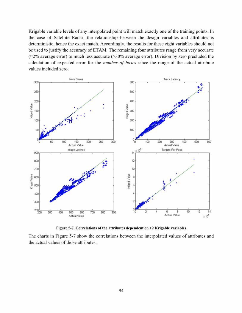
94

Krigable variable levels of any interpolated point will match exactly one of the training points. In the case of Satellite Radar, the relationship between the design variables and attributes is deterministic, hence the exact match. Accordingly, the results for these eight variables should not be used to justify the accuracy of ETAM. The remaining four attributes range from very accurate (≈2% average error) to much less accurate (>30% average error). Division by zero precluded the calculation of expected error for the number of boxes since the range of the actual attribute values included zero.

Figure 5-7. Correlations of the attributes dependent on >2 Krigable variables

The charts in Figure 5-7 show the correlations between the interpolated values of attributes and the actual values of those attributes.

95

Figure 5-8. Error distributions of the attributes dependent on >2 Krigable variables

Figure 5-8 shows the corresponding error distributions. For some attributes, the error seems to be distributed evenly about the actual value. For others, such as number of boxes (top-left), the error seems to be more systematic. For number of boxes, the Kriged values tend to be higher than the actual value for low actual values. For higher actual values, the Kriged value tends to underestimate the actual value. This due to the fact that there are very few (relative to the all the designs) values for the number of boxes attribute above 100 boxes. If the training set for that specific Krigable subset only captured one high value, an instance where the actual value should be high will always be underestimated; even though the design-epoch vector of the point to be interpolated might be closest to the high value point’s design-epoch vector, the value will be discounted by the surrounding points of lesser values (discounted by distance). This pattern does not carry over to the targets per pass attribute, as seen by the overestimates for higher (and less frequent) values in the lower right figure. Here the large scattering about the actual value is due to the small Kriging errors being propagated through the logarithmic transformation.

In many tradespace studies, multi-attribute utility (MAU) is used to evaluate design options (Keeney and Raiffa 1993). For this study, MAU value is calculated as a weighted sum, according

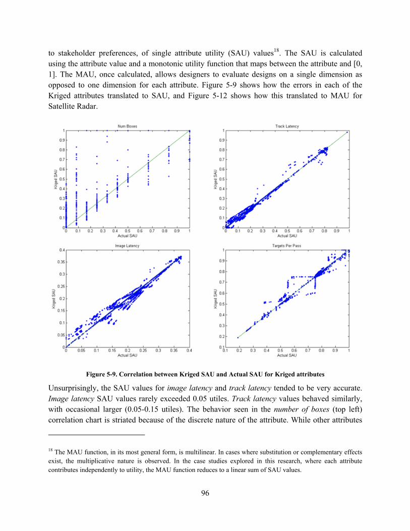
96

to stakeholder preferences, of single attribute utility (SAU) values18. The SAU is calculated using the attribute value and a monotonic utility function that maps between the attribute and [0, 1]. The MAU, once calculated, allows designers to evaluate designs on a single dimension as opposed to one dimension for each attribute. Figure 5-9 shows how the errors in each of the Kriged attributes translated to SAU, and Figure 5-12 shows how this translated to MAU for Satellite Radar.

Figure 5-9. Correlation between Kriged SAU and Actual SAU for Kriged attributes

Unsurprisingly, the SAU values for image latency and track latency tended to be very accurate. Image latency SAU values rarely exceeded 0.05 utiles. Track latency values behaved similarly, with occasional larger (0.05-0.15 utiles). The behavior seen in the number of boxes (top left) correlation chart is striated because of the discrete nature of the attribute. While other attributes

18 The MAU function, in its most general form, is multilinear. In cases where substitution or complementary effects exist, the multiplicative nature is observed. In the case studies explored in this research, where each attribute contributes independently to utility, the MAU function reduces to a linear sum of SAU values.

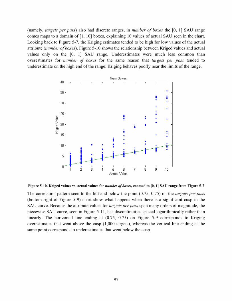
97

(namely, targets per pass) also had discrete ranges, in number of boxes the [0, 1] SAU range comes maps to a domain of [1, 10] boxes, explaining 10 values of actual SAU seen in the chart. Looking back to Figure 5-7, the Kriging estimates tended to be high for low values of the actual attribute (number of boxes). Figure 5-10 shows the relationship between Kriged values and actual values only on the [0, 1] SAU range. Underestimates were much less common than overestimates for number of boxes for the same reason that targets per pass tended to underestimate on the high end of the range: Kriging behaves poorly near the limits of the range.

Figure 5-10. Kriged values vs. actual values for number of boxes, zoomed to [0, 1] SAU range from Figure 5-7

The correlation pattern seen to the left and below the point (0.75, 0.75) on the targets per pass (bottom right of Figure 5-9) chart show what happens when there is a significant cusp in the SAU curve. Because the attribute values for targets per pass span many orders of magnitude, the piecewise SAU curve, seen in Figure 5-11, has discontinuities spaced logarithmically rather than linearly. The horizontal line ending at (0.75, 0.75) on Figure 5-9 corresponds to Kriging overestimates that went above the cusp (1,000 targets), whereas the vertical line ending at the same point corresponds to underestimates that went below the cusp.

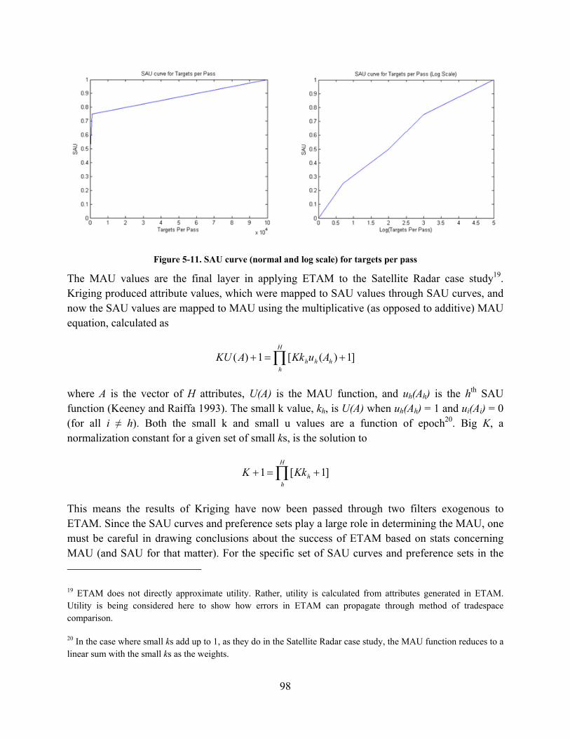
98

Figure 5-11. SAU curve (normal and log scale) for targets per pass

The MAU values are the final layer in applying ETAM to the Satellite Radar case study19. Kriging produced attribute values, which were mapped to SAU values through SAU curves, and now the SAU values are mapped to MAU using the multiplicative (as opposed to additive) MAU equation, calculated as

]1)([1)( h

H

hhh AuKkAKU

where A is the vector of H attributes, U(A) is the MAU function, and uh(Ah) is the hth SAU function (Keeney and Raiffa 1993). The small k value, kh, is U(A) when uh(Ah) = 1 and ui(Ai) = 0 (for all i ≠ h). Both the small k and small u values are a function of epoch20. Big K, a normalization constant for a given set of small ks, is the solution to

]1[1

H

hhKkK

This means the results of Kriging have now been passed through two filters exogenous to ETAM. Since the SAU curves and preference sets play a large role in determining the MAU, one must be careful in drawing conclusions about the success of ETAM based on stats concerning MAU (and SAU for that matter). For the specific set of SAU curves and preference sets in the

19 ETAM does not directly approximate utility. Rather, utility is calculated from attributes generated in ETAM. Utility is being considered here to show how errors in ETAM can propagate through method of tradespace comparison.

20 In the case where small ks add up to 1, as they do in the Satellite Radar case study, the MAU function reduces to a linear sum with the small ks as the weights.

99

each epoch, Figure 5-12 shows how the Kriged MAU values corresponded to actual MAU values for Satellite Radar. One of the main reasons Kriging overestimated MAU more than it underestimated MAU was the fact that number of boxes was heavily overestimated and happened to be one of the highest weighted attributes (highest small k).

Figure 5-12. Correlation between Kriged MAU and Actual MAU for Satellite Radar

As mentioned above, analysis of SAU and MAU data must be done carefully to account for the fact that SAU curves and MAU preference sets have an impact. Statistics like percent error and average error can be misleading. For example, a 3% error for an actual MAU of 0.1 is much different than a 3% error when the actual MAU is 1. Similarly, an error of 0.01 utiles might mean less near the middle of the utility range whereas if it saturates a MAU to 1 it means much more. While percent error and average error might be misleading statistics for SAU and MAU data, a metric that looks only at ordering is more appropriate. The Spearman’s rank correlation coefficient (Spaulding 2003) was used to characterize the accuracy of DOE-Kriging on the individual SAU values and MAU. The Spearman’s rank correlation coefficient measures the correlation between the ranks of a value in two different sets, in this case a design’s actual MAU/SAU value and its Kriged MAU/SAU value. For each epoch, a Spearman’s coefficient was calculated for the four Kriged attributes’ SAU values as well as the MAU. The values were then averaged over all epochs and can be seen in Table 5-8. Little variance was seen in Spearman coefficients across epochs. The insight gained from the relatively high Spearman’s coefficients is that little accuracy is lost with respect to relative performance (a Spearman’s coefficient of 1 implies rank is completely preserved). The significance of this test was very strong due to the extremely large sample size.

100

Table 5-8. Spearman's Rank Correlation Coefficients for SAU and MAU Values

Value SAU(Number of Boxes)

SAU(Track Latency)

SAU(Image Latency)

SAU(Targets per Pass)

MAU

Spearman’s Coefficient

0.8705 0.9959 0.9574 0.9738 0.9720

5.4 Application to Space Tug

The Space Tug data set contains designs for orbital transfer vehicles that can be used for a variety of on-orbit servicing missions such as observation of (potentially hostile) targets, assisting in orbit changes, and removing debris (McManus and Schuman 2003). This data set has been used for studies in changeability and survivability (Richards 2009, Ross and Hastings 2006). Recent work has added context variables to the existing preference curves used to define the epochs.

5.4.1 Variable Handling

For Space Tug, the design variables originally introduced are manipulator size, propulsion system, and fuel mass. An additional variable, design for evolvability (DfE), was added for the purposes of this simulation. The DfE variable represents the inclusion of design heuristics that make redesign simpler and is treated as a mass penalty. The ranges of values for the design variables are seen in Figure 5-10. All of the design variables except for propulsion system will be considered Krigable variables. The product of the levels of all Krigable variables for Space Tug is 96.

101

Table 5-9. Design Variable Levels (McManus and Schuman 2003, Fulcoly et al. 2012) Krigable Variables are Italicized

Design Variable Scale Type

Valid Range Enumerated Levels # Levels

Manipulator Mass Ratio 300 – 5000 [kg] 300, 1000, 3000, 5000 [kg]

4

Propulsion System Nominal 1 – 4 [int] Storable BiPropellant, Cryogenic, Electric, Nuclear

4

Fuel Mass Ratio 300 – 30000 [kg] 30, 100, 300, 600, 1200, 3000, 10000, 30000 [kg]

8

DfE Mass Penalty Ratio 0 – 20 [%] 0, 10, 20 [%] 3

Only one of the Space Tug epoch variables, technology level, will be used for testing ETAM. Technology is either “present level” or “future level” and affects the attribute levels associated with each design variable as well as the cost calculation. The attribute levels are then used to calculate utility. Since technology level is a nominal variable, it will be treated as non-Krigable.

The three attributes originally calculated were capability, delta V, and response time. Capability is measured as the manipulator mass. Delta V is a function of all masses, specific impulse, and mass fraction. The latter two are properties of the propulsion system in use, as seen in Table 5-10. In cases where two values appear, the latter value is used in the future context. Response time is either fast or slow and is a function solely of the propulsion and is in the ‘Fast?’ column of Table 5-10.

Table 5-10. Propulsion System Values (McManus and Schuman 2003)

Propulsion System Isp (sec) Base Mass (kg) Mass Fraction Fast? Storable Bipropellant 300 0 0.12 Y Cryo 450/550 0 0.13 Y Electric 3000 25 0.25/0.3 N Nuclear 1500 1000/600 0.20 Y

The cost of a design is a function of its dry and wet mass. First, the propulsion system mass (Mp) must be calculated using base mass (mp0), mass fraction (mpf), and the fuel mass (Mf)

fpfpp MmmM 0

102

Next, the vehicle bus mass (Mb) is calculated using the propulsion system mass, manipulator mass (Mm), and bus mass fraction (mbf)

mbfpb MmMM

The bus mass fraction was held constant at 1 for this case study. The mass penalty for DfE is levied in the final mass calculations. The vehicle dry mass (Md) and vehicle wet mass (Mw) then are calculated as

fdw

mbd

MMM

MMDfEM

)1(

The dry mass cost (cd) of $150,000/kg and the wet mass cost (cw) of $15,000/kg in the present context ($10,000/kg in the future context) is used to calculate cost (C)21,22

ddww McMcC

Delta V is calculated as

d

wdsp M

MMIv ln

Because response time is a function of only a non-Krigable variable, it will not be considered in this application of ETAM. Using the attribute functions, the binary DMM can be created. The Binary DMM, shown in Table 5-11 reveals that both attributes are a function of each of the Krigable variables, therefore only one training set will need to be used.

21 These cost values were adapted from McManus and Schuman (2003). The future context wet mass cost was proposed by MIT student Matt Fitzgerald.

22 The cost model for Space Tug was readily available, unlike Satellite Radar, hence it being considered an attribute in the former but not the latter.

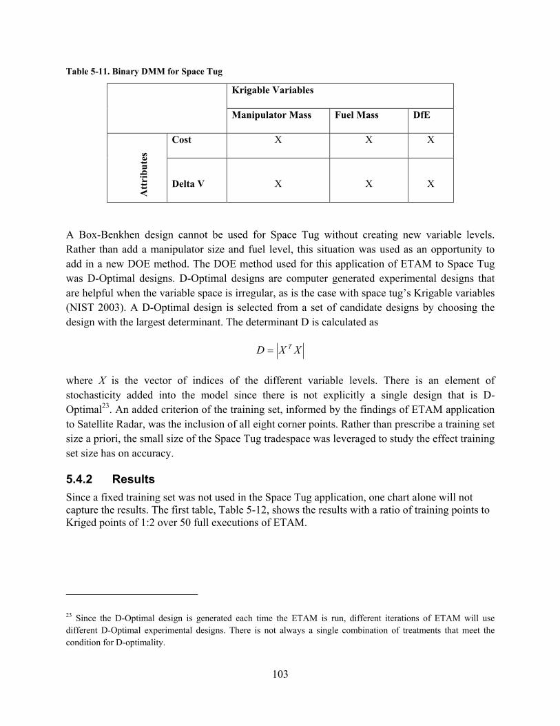
103

Table 5-11. Binary DMM for Space Tug

Krigable Variables

Manipulator Mass Fuel Mass DfE

Att

rib

ute

s Cost X X X

Delta V X X X

A Box-Benkhen design cannot be used for Space Tug without creating new variable levels. Rather than add a manipulator size and fuel level, this situation was used as an opportunity to add in a new DOE method. The DOE method used for this application of ETAM to Space Tug was D-Optimal designs. D-Optimal designs are computer generated experimental designs that are helpful when the variable space is irregular, as is the case with space tug’s Krigable variables (NIST 2003). A D-Optimal design is selected from a set of candidate designs by choosing the design with the largest determinant. The determinant D is calculated as

XXD T

where X is the vector of indices of the different variable levels. There is an element of stochasticity added into the model since there is not explicitly a single design that is D-Optimal23. An added criterion of the training set, informed by the findings of ETAM application to Satellite Radar, was the inclusion of all eight corner points. Rather than prescribe a training set size a priori, the small size of the Space Tug tradespace was leveraged to study the effect training set size has on accuracy.

5.4.2 Results

Since a fixed training set was not used in the Space Tug application, one chart alone will not capture the results. The first table, Table 5-12, shows the results with a ratio of training points to Kriged points of 1:2 over 50 full executions of ETAM.

23 Since the D-Optimal design is generated each time the ETAM is run, different iterations of ETAM will use different D-Optimal experimental designs. There is not always a single combination of treatments that meet the condition for D-optimality.

104

Table 5-12. Accuracy of Kriged Variables (32 Training Points) Over 50 Full Executions of ETAM

Attribute Mean (Training Set Points) E[|Difference|] Std[|Difference|]

Average Error

Spearman Rho

Cost $976,640,000 $3,722,500 $5,368,500 0.55% 0.9999

Delta V 5.2437 km/s 0.898 km/s 1.6964 km/s 0.29% 0.9617

A first order examination shows that ETAM was accurate within a percent for both cost and delta V. The Spearman rho values, which represent the rank correlation coefficient, reveal that order is very well preserved in cost and less so in delta V. This relationship, for a single execution of ETAM, can be seen in Figure 5-13.

Figure 5-13. Cost and Delta V Correlations and Error Distributions for 32 Training Points

The Spearman rho for cost is nearly one, and tended to be so for any number of training points. The Spearman rho values for delta V, on the other hand, were much more sensitive to the size of the training set, as seen in Figure 5-14.

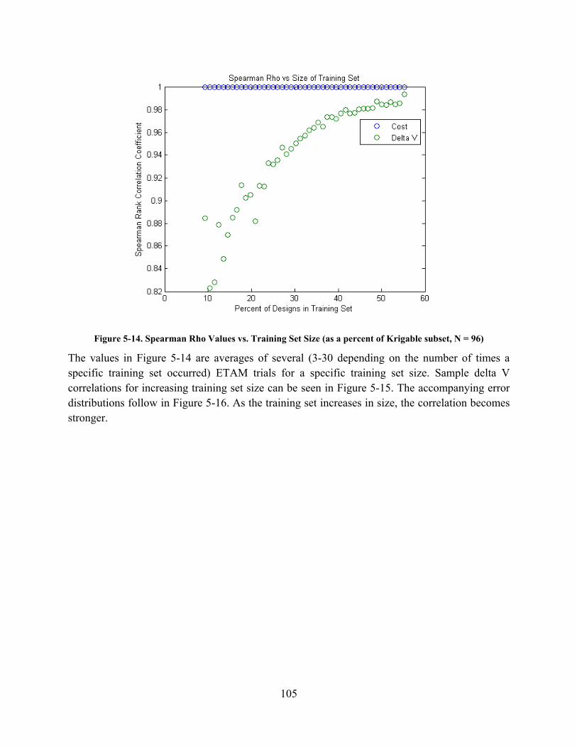
105

Figure 5-14. Spearman Rho Values vs. Training Set Size (as a percent of Krigable subset, N = 96)

The values in Figure 5-14 are averages of several (3-30 depending on the number of times a specific training set occurred) ETAM trials for a specific training set size. Sample delta V correlations for increasing training set size can be seen in Figure 5-15. The accompanying error distributions follow in Figure 5-16. As the training set increases in size, the correlation becomes stronger.

106

Figure 5-15. Correlation of Kriged vs. Actual Delta V Values for Different Training Set Sizes (Clockwise from top left: 17, 25, 40, 51)

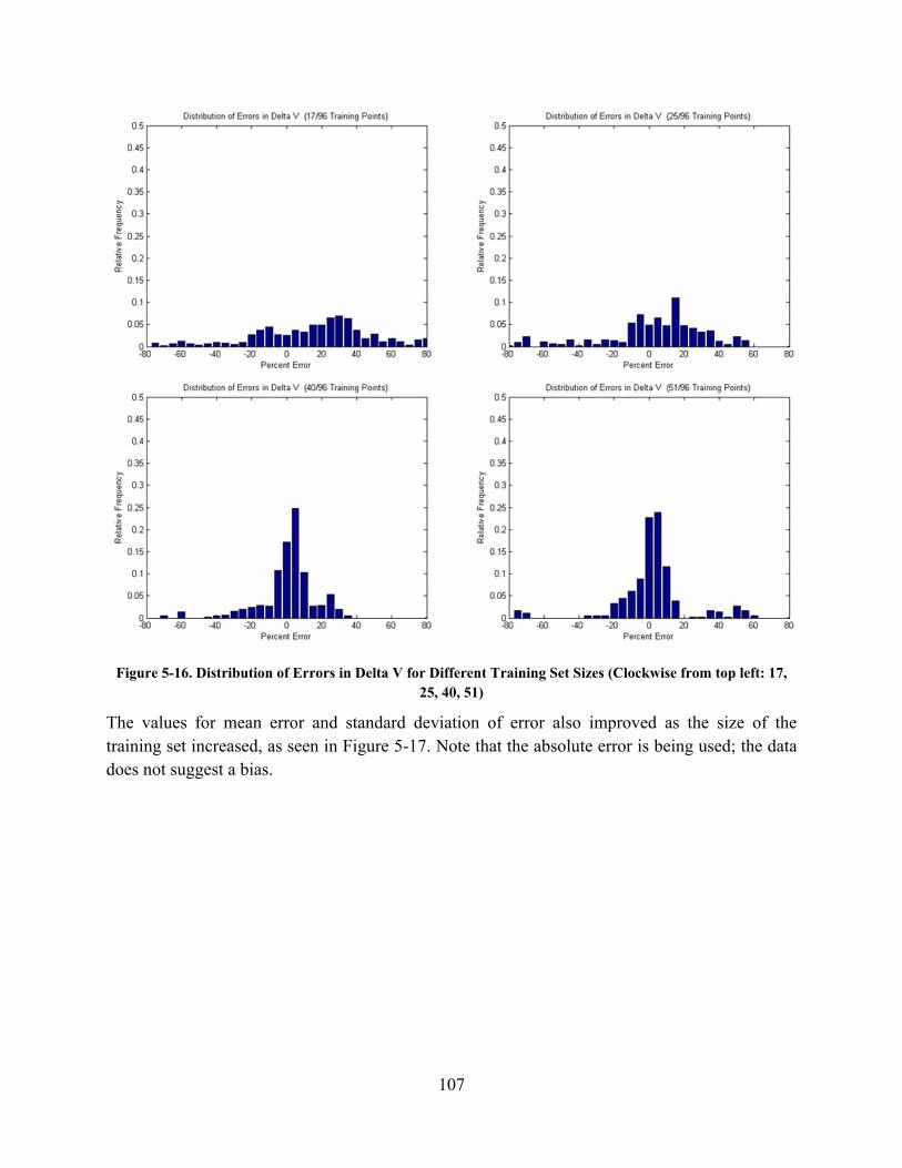
107

Figure 5-16. Distribution of Errors in Delta V for Different Training Set Sizes (Clockwise from top left: 17, 25, 40, 51)

The values for mean error and standard deviation of error also improved as the size of the training set increased, as seen in Figure 5-17. Note that the absolute error is being used; the data does not suggest a bias.

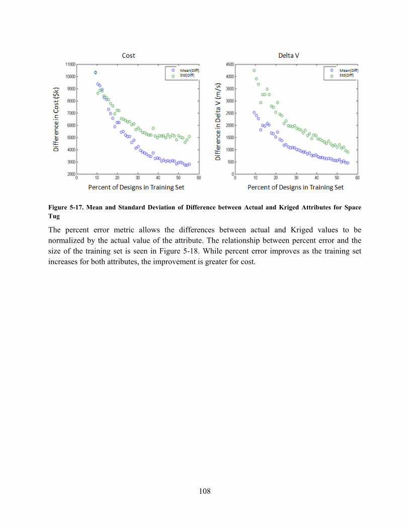
108

Figure 5-17. Mean and Standard Deviation of Difference between Actual and Kriged Attributes for Space Tug

The percent error metric allows the differences between actual and Kriged values to be normalized by the actual value of the attribute. The relationship between percent error and the size of the training set is seen in Figure 5-18. While percent error improves as the training set increases for both attributes, the improvement is greater for cost.

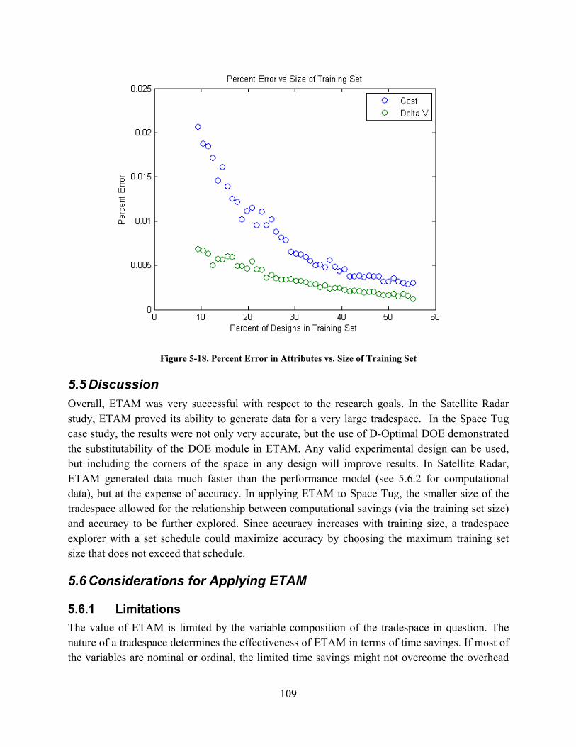
109

Figure 5-18. Percent Error in Attributes vs. Size of Training Set

5.5 Discussion Overall, ETAM was very successful with respect to the research goals. In the Satellite Radar study, ETAM proved its ability to generate data for a very large tradespace. In the Space Tug case study, the results were not only very accurate, but the use of D-Optimal DOE demonstrated the substitutability of the DOE module in ETAM. Any valid experimental design can be used, but including the corners of the space in any design will improve results. In Satellite Radar, ETAM generated data much faster than the performance model (see 5.6.2 for computational data), but at the expense of accuracy. In applying ETAM to Space Tug, the smaller size of the tradespace allowed for the relationship between computational savings (via the training set size) and accuracy to be further explored. Since accuracy increases with training size, a tradespace explorer with a set schedule could maximize accuracy by choosing the maximum training set size that does not exceed that schedule.

5.6 Considerations for Applying ETAM

5.6.1 Limitations

The value of ETAM is limited by the variable composition of the tradespace in question. The nature of a tradespace determines the effectiveness of ETAM in terms of time savings. If most of the variables are nominal or ordinal, the limited time savings might not overcome the overhead

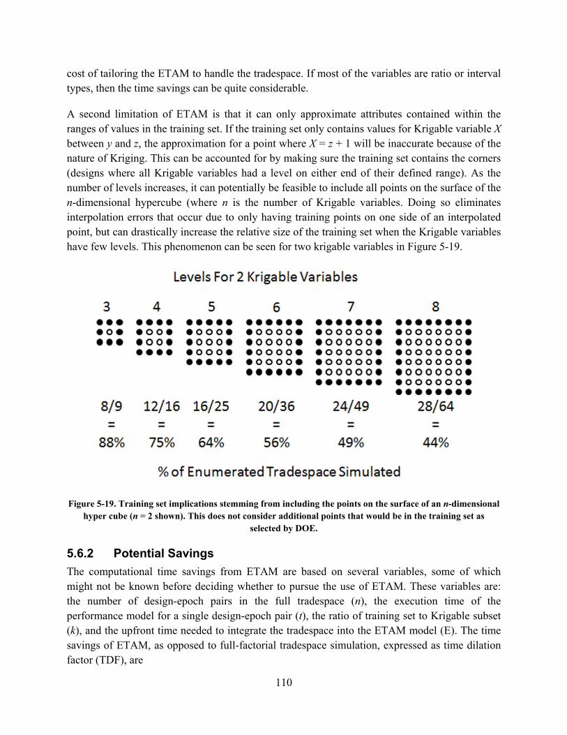
110

cost of tailoring the ETAM to handle the tradespace. If most of the variables are ratio or interval types, then the time savings can be quite considerable.

A second limitation of ETAM is that it can only approximate attributes contained within the ranges of values in the training set. If the training set only contains values for Krigable variable X between y and z, the approximation for a point where X = z + 1 will be inaccurate because of the nature of Kriging. This can be accounted for by making sure the training set contains the corners (designs where all Krigable variables had a level on either end of their defined range). As the number of levels increases, it can potentially be feasible to include all points on the surface of the n-dimensional hypercube (where n is the number of Krigable variables. Doing so eliminates interpolation errors that occur due to only having training points on one side of an interpolated point, but can drastically increase the relative size of the training set when the Krigable variables have few levels. This phenomenon can be seen for two krigable variables in Figure 5-19.

Figure 5-19. Training set implications stemming from including the points on the surface of an n-dimensional hyper cube (n = 2 shown). This does not consider additional points that would be in the training set as

selected by DOE.

5.6.2 Potential Savings

The computational time savings from ETAM are based on several variables, some of which might not be known before deciding whether to pursue the use of ETAM. These variables are: the number of design-epoch pairs in the full tradespace (n), the execution time of the performance model for a single design-epoch pair (t), the ratio of training set to Krigable subset (k), and the upfront time needed to integrate the tradespace into the ETAM model (E). The time savings of ETAM, as opposed to full-factorial tradespace simulation, expressed as time dilation factor (TDF), are

111

100

tn

tnkETDF

A TDF of 100% means using ETAM takes the same amount of time as simulating the full tradespace. A TDF below 100% means time was saved by using ETAM and a TDF greater than 100% means ETAM takes longer than simulating the full tradespace would have taken. As the time needed to simulate the full tradespace becomes much greater than the anticipated ETAM setup time (nt >> E), the TDF approaches 100*k. When E ≈ nt, the TDF is approximately -100*(1+k). When E >> nt, the TDF approaches 100*(E/nt). As a general rule, ETAM should only be used if nt >> E.

Table 5-13. Time Dilation Factor for Different Case Studies24

Case Study E k n t Time Dilation Factor Satellite Radar 8 hours 13/81 6,718,464 ≈26s 16.07% Space Tug 2 hours 32/96 384 0.0015s 1,250,000%

The advantage from ETAM in each case study can be seen in Table 5-13. The very poor time dilation factor for the Space Tug case study is expected since the full tradespace was very small and the performance model was very simple; Space Tug was used to demonstrate the accuracy of ETAM and not to showcase its effectiveness in saving time.

5.6.3 Potential Costs

The computational savings of ETAM must be weighed against the costs incurred in accuracy. ETAM displayed varying levels of accuracy for the four Kriged attributes in Satellite Radar (as seen in Table 5-7, Figure 5-7, Figure 5-8, and Table 5-8) when only simulating 16% of the enumerated tradespace. For the Space Tug case study, it was clearly demonstrated that the accuracy increases with the percent of designs simulated (as seen in Figure 5-14, Figure 5-15’ Figure 5-16, Figure 5-17, and Figure 5-18). Ultimately, it is up to the tradespace explorer to determine the amount of potential accuracy they are willing to sacrifice for computational savings. At this point there is no way to approximate accuracy losses, but application to further case studies might lead towards more insights concerning such losses.

24 The t value for Satellite Radar was estimated based on anecdotal evidence from the original simulation operators based on the following values: 23,778 designs, 972 epochs, ≈10 days to simulate.

112

113

6 Discussion

6.1 Revisiting Research Questions Recall the five research questions proposed in chapter 1:

1. What is evolvability in the context of systems engineering? 2. How can evolvability be designed into a system? 3. How does timing affect system changes? 4. Under what conditions is it appropriate to design evolvability into a system? 5. Is there a way to make exploring very large tradespaces more feasible when facing computational

constraints?

Evolvability was defined in chapter 2.1 to be “the ability of an architecture to be inherited and changed across generations [over time].” The definition itself “evolved” several times over the course of research contributing to this thesis. As the research team gained more experience working in the systems engineering field and explored more literature, the definition tended to change in order to better relate to existing concepts of evolvability and better capture the SEAri concept of evolvability25. One of the first evolvability definitions proposed in this research was “The ability to change the state of a family of systems in a realizable subset of a possible parameter space through some regulated process of variation and selection across generations.” The motivation for a definition of this type was to maintain relation to the biological concept of evolution, what comes to mind for most people when evolvability is mentioned. This can be seen in the definition when variation and selection are mentioned. Variation in engineering was concept generation, early trade studies, etc. whereas selection was picking the most “fit” design through some method of analysis. The two biological concepts that are maintained in the current definition of evolvability are generations and inheritance (variation and selection are no longer explicitly mentioned, although as stated before they are implicitly present in the way redesign often occurs). It was discovered that the first definition was too specific and difficult to apply.

The second, third, and fourth research questions both relate to design principles. The insights gained with respect to these questions are seen in 6.1.1. The fifth research question was addressed by ETAM and is discussed in 6.1.2.

6.1.1 Design Principles

Recall from chapter 2.2.2 that several design principles were found in existing evolvability, changeability, and flexibility literature. These design principles can be seen in Table 6-1. Unfortunately there was no explicit effort in this research to test each design principle in this list;

25 Evolvability was not the subject of significant research in SEAri prior to the beginning of this research. As such, the concept of evolvability as it related to other ilities changed and matured during the course of this research.

114

to do so would require a case study that explicitly or implicitly includes each one of them. When a case study does include one or more of these design principles, inferences can be made about the value of that design principle. Future work should address this approach.

Table 6-1. Existing Design Principles for Evolvability

Design Principle Proposed by Modularity Holtta-Otto (2005), Hansen (2003), Christian (2005), Integrability/Common Interfaces Fricke and Schulz (2003), Christian (2005), Holtta-Otto (2005) Interoperability Christian (2005) Scalability Fricke and Schulz (2003) Reconfigurability Siddiqi and de Weck (2008) Margin Christian (2005), Silver and de Weck (2007) Architecture Changeability Ross (2006)

Modularity is seen in a considerable number of papers in the systems engineering literature as a design principle for many ilities. It was realized, however, that modularity in all aspects of a system might not be necessary or even beneficial. Only a certain degree of modularity might be needed. For example, if a system has components A, B, C, and D, but technology and requirements concerning A and B are constant and show no signs of changing, leaving A and B coupled will not hinder evolution. The concept of only using modularity in certain components or subsystems is called targeted modularity. Another design principle that was proposed during informal discussions with members of the systems engineering community was proper documentation26. When the redesign team is composed of different members than the original design team, sometimes documentation is all that exists for them to work from (especially if they do not have access to former team members). By capturing as much information as possible in documentation, even if takes more time and is more expensive, the evolvable redesign process might be less difficult and provide a positive return on the extra resources spent on documentation.

In addition to design principles for including evolvability, some literature included considerations for when including evolvability in a system is appropriate. Nam Pyo Suh (1990) suggests that a long product development cycle (with respect to changing epoch variables like demand) might lead to a system being obsolete. Fricke and Schulz (2003) explain how a system should have evolvability27 when the system has a long lifecycle with respect to the cycle times of

26 These discussions occurred at the 2012 Conference for Systems Engineering Research (CSER) at St. Louis, MO in March 2012.

27 The authors use “changeability” in their work, but their changeability is considered “evolvability” in this discussion based on their definitions.

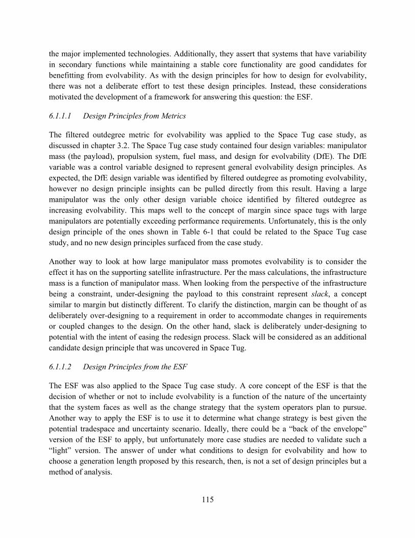
115

the major implemented technologies. Additionally, they assert that systems that have variability in secondary functions while maintaining a stable core functionality are good candidates for benefitting from evolvability. As with the design principles for how to design for evolvability, there was not a deliberate effort to test these design principles. Instead, these considerations motivated the development of a framework for answering this question: the ESF.

6.1.1.1 Design Principles from Metrics

The filtered outdegree metric for evolvability was applied to the Space Tug case study, as discussed in chapter 3.2. The Space Tug case study contained four design variables: manipulator mass (the payload), propulsion system, fuel mass, and design for evolvability (DfE). The DfE variable was a control variable designed to represent general evolvability design principles. As expected, the DfE design variable was identified by filtered outdegree as promoting evolvability, however no design principle insights can be pulled directly from this result. Having a large manipulator was the only other design variable choice identified by filtered outdegree as increasing evolvability. This maps well to the concept of margin since space tugs with large manipulators are potentially exceeding performance requirements. Unfortunately, this is the only design principle of the ones shown in Table 6-1 that could be related to the Space Tug case study, and no new design principles surfaced from the case study.

Another way to look at how large manipulator mass promotes evolvability is to consider the effect it has on the supporting satellite infrastructure. Per the mass calculations, the infrastructure mass is a function of manipulator mass. When looking from the perspective of the infrastructure being a constraint, under-designing the payload to this constraint represent slack, a concept similar to margin but distinctly different. To clarify the distinction, margin can be thought of as deliberately over-designing to a requirement in order to accommodate changes in requirements or coupled changes to the design. On the other hand, slack is deliberately under-designing to potential with the intent of easing the redesign process. Slack will be considered as an additional candidate design principle that was uncovered in Space Tug.

6.1.1.2 Design Principles from the ESF

The ESF was also applied to the Space Tug case study. A core concept of the ESF is that the decision of whether or not to include evolvability is a function of the nature of the uncertainty that the system faces as well as the change strategy that the system operators plan to pursue. Another way to apply the ESF is to use it to determine what change strategy is best given the potential tradespace and uncertainty scenario. Ideally, there could be a “back of the envelope” version of the ESF to apply, but unfortunately more case studies are needed to validate such a “light” version. The answer of under what conditions to design for evolvability and how to choose a generation length proposed by this research, then, is not a set of design principles but a method of analysis.

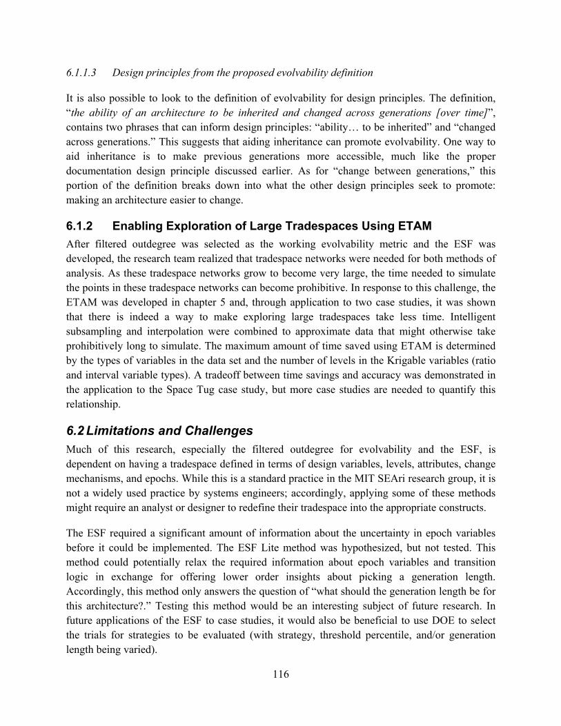
116

6.1.1.3 Design principles from the proposed evolvability definition

It is also possible to look to the definition of evolvability for design principles. The definition, “the ability of an architecture to be inherited and changed across generations [over time]”, contains two phrases that can inform design principles: “ability… to be inherited” and “changed across generations.” This suggests that aiding inheritance can promote evolvability. One way to aid inheritance is to make previous generations more accessible, much like the proper documentation design principle discussed earlier. As for “change between generations,” this portion of the definition breaks down into what the other design principles seek to promote: making an architecture easier to change.

6.1.2 Enabling Exploration of Large Tradespaces Using ETAM

After filtered outdegree was selected as the working evolvability metric and the ESF was developed, the research team realized that tradespace networks were needed for both methods of analysis. As these tradespace networks grow to become very large, the time needed to simulate the points in these tradespace networks can become prohibitive. In response to this challenge, the ETAM was developed in chapter 5 and, through application to two case studies, it was shown that there is indeed a way to make exploring large tradespaces take less time. Intelligent subsampling and interpolation were combined to approximate data that might otherwise take prohibitively long to simulate. The maximum amount of time saved using ETAM is determined by the types of variables in the data set and the number of levels in the Krigable variables (ratio and interval variable types). A tradeoff between time savings and accuracy was demonstrated in the application to the Space Tug case study, but more case studies are needed to quantify this relationship.

6.2 Limitations and Challenges Much of this research, especially the filtered outdegree for evolvability and the ESF, is dependent on having a tradespace defined in terms of design variables, levels, attributes, change mechanisms, and epochs. While this is a standard practice in the MIT SEAri research group, it is not a widely used practice by systems engineers; accordingly, applying some of these methods might require an analyst or designer to redefine their tradespace into the appropriate constructs.

The ESF required a significant amount of information about the uncertainty in epoch variables before it could be implemented. The ESF Lite method was hypothesized, but not tested. This method could potentially relax the required information about epoch variables and transition logic in exchange for offering lower order insights about picking a generation length. Accordingly, this method only answers the question of “what should the generation length be for this architecture?.” Testing this method would be an interesting subject of future research. In future applications of the ESF to case studies, it would also be beneficial to use DOE to select the trials for strategies to be evaluated (with strategy, threshold percentile, and/or generation length being varied).

117

7 Conclusions This research explored many methods surrounding the topic of evolvability in systems engineering. In the process of searching for a normative set of evolvability design principles, evolvability was defined, existing design principles were examined, a metric for evolvability was derived from a set of candidate metrics, a method for examining the temporal aspects of changes over a system lifecycle was developed and demonstrated, and a method was developed for approximating large tradespaces to expand the set of case studies that can be examined using evolvability metrics and the ESF. Over the course of the research, the emphasis shifted from extracting general design principles to developing methods to enable the extraction of design principles. The design principles that were identified, either from existing literature or new research, are seen in Table 7-1

Table 7-1. Candidate Design Principles for Evolvability

Design Principle Proposed by Comments Targeted Modularity Holtta-Otto (2005), Hansen (2003),

Christian (2005), Fulcoly (2012) Originally modularity, targeted modularity proposed in this thesis

Integrability/Common Interfaces

Fricke and Schulz (2003), Christian (2005), Holtta-Otto (2005)

Interoperability Christian (2005) Scalability Fricke and Schulz (2003) Reconfigurability Siddiqi and de Weck (2008) Margin Christian (2005), Silver and de

Weck (2007), Fulcoly (2012) Identified in application of filtered outdegree to Space Tug case study

Architecture Changeability Ross (2006) Proper Documentation Fulcoly (2012) Proposed in this thesis Slack Fulcoly (2012) Proposed in this thesis 

7.1 Contributions

There are three main contributions of this research to the field of systems engineering: the filtered outdegree as a preferred metric for measuring evolvability, the Epoch Syncopation Framework (ESF) as a method for analyzing both how timing affects system changes and under what conditions it is appropriate to design for evolvability, and the Expedited Tradespace Approximation Method (ETAM) as an enabler for studying evolvability by making very large tradespaces accessible for analysis.

The filtered outdegree for evolvability metric treats a tradespace as a network of design points connected by arcs representing evolvable change mechanisms associated with a change cost and schedule impact, as seen in Figure 7-1. The number of designs reachable by arcs below a certain resource threshold from a given design is the filtered outdegree for that design. This metric is

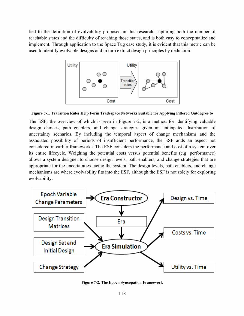
118

tied to the definition of evolvability proposed in this research, capturing both the number of reachable states and the difficulty of reaching those states, and is both easy to conceptualize and implement. Through application to the Space Tug case study, it is evident that this metric can be used to identify evolvable designs and in turn extract design principles by deduction.

Figure 7-1. Transition Rules Help Form Tradespace Networks Suitable for Applying Filtered Outdegree to

The ESF, the overview of which is seen in Figure 7-2, is a method for identifying valuable design choices, path enablers, and change strategies given an anticipated distribution of uncertainty scenarios. By including the temporal aspect of change mechanisms and the associated possibility of periods of insufficient performance, the ESF adds an aspect not considered in earlier frameworks. The ESF considers the performance and cost of a system over its entire lifecycle. Weighing the potential costs versus potential benefits (e.g. performance) allows a system designer to choose design levels, path enablers, and change strategies that are appropriate for the uncertainties facing the system. The design levels, path enablers, and change mechanisms are where evolvability fits into the ESF, although the ESF is not solely for exploring evolvability.

Figure 7-2. The Epoch Syncopation Framework

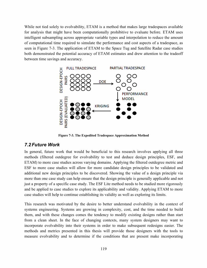
119

While not tied solely to evolvability, ETAM is a method that makes large tradespaces available for analysis that might have been computationally prohibitive to evaluate before. ETAM uses intelligent subsampling across appropriate variable types and interpolation to reduce the amount of computational time required to simulate the performance and cost aspects of a tradespace, as seen in Figure 7-3. The application of ETAM to the Space Tug and Satellite Radar case studies both demonstrated the potential accuracy of ETAM estimates and drew attention to the tradeoff between time savings and accuracy.

Figure 7-3. The Expedited Tradespace Approximation Method

7.2 Future Work In general, future work that would be beneficial to this research involves applying all three methods (filtered outdegree for evolvability to test and deduce design principles, ESF, and ETAM) to more case studies across varying domains. Applying the filtered outdegree metric and ESF to more case studies will allow for more candidate design principles to be validated and additional new design principles to be discovered. Showing the value of a design principle via more than one case study can help ensure that the design principle is generally applicable and not just a property of a specific case study. The ESF Lite method needs to be studied more rigorously and be applied to case studies to explore its applicability and validity. Applying ETAM to more case studies will help to continue establishing its validity as well as exploring its limits.

This research was motivated by the desire to better understand evolvability in the context of systems engineering. Systems are growing in complexity, cost, and the time needed to build them, and with these changes comes the tendency to modify existing designs rather than start from a clean sheet. In the face of changing contexts, many system designers may want to incorporate evolvability into their systems in order to make subsequent redesigns easier. The methods and metrics presented in this thesis will provide those designers with the tools to measure evolvability and to determine if the conditions that are present make incorporating

120

evolvability appropriate. The methods and metrics can also help determine if preplanned generations should be used (including what the generation length should be) in addition to providing a means with which to discover and test design principles for evolvability. Finally, in the event that the tradespace in question is very large, ETAM gives designers the ability to consider more of the tradespace within the computational resources available to them.

121

8 References

Balabanov, V.O., Charpentier, C., Ghosh, D., Quin, G., Vanderplaats, G.N., “VisualDOC: A Software System for General-Purpose Integration and Design Optimization,” 9th AIAA/ISSMO Symposium on Multidisciplinary Analysis and Optimization, Atlanta, GA, Sept. 2002.

Beesemyer J.C., Fulcoly D.O., Rhodes D.H., Ross A.M., “Developing methods to design for evolvability: research approach and preliminary design principles,” proceedings of the 9th Conference on Systems Engineering Research, Los Angeles, CA, April 2011.

Beesemyer, J.C., Ross, A.M., and Rhodes, D.H., "Empirical Examples of System Changes to Frame Links between Design Decisions and Ilities," 10th Conference on Systems Engineering Research, St. Louis, MO, March 2012.

Borches, P.D., and Bonnema, G.M., “Coping with System Evolution-Experiences in Reverse Architecting as a Means to Ease the Evolution of Complex Systems,” 19th International Symposium of Systems Engineering, Singapore, July 2009.

Box, G.E.P., and Benkhen, D. W., “Some New Three Level Designs for the Study of Quantitative Variables”. Technometrics, Vol. 2, 1960, pp. 455-475.

Browning, T.R., “Applying the Design Structure Matrix to System Decomposition and Integration Problems: A Review and New Directions,” IEEE Transactions on Engineering Management, 2001:48(3):292-306.

Cardin, M.A., Quantitative performance-based evaluation of a procedure for flexible design concept generation, Doctor of Philosophy Dissertation, Engineering Systems Division, MIT, June 2011.

Chiles, J.P., and Delfiner, P., Geostatistics: Modeling Spatial Uncertainty, Wiley Interscience, New York, 1999, pp. 150-192.

Christian III, J.A., “A Quantitative Approach to Assessing System Evolvability,” Systems Engineering. 2004;(770):1-16.

Christian III, J.A., and Olds, J.R., “A Quantitative Methodology for Identifying Evolvable Space Systems,” AIAA Space Exploration Conference, Orlando, FL, February 2005.

Dahmann, J., Rebovich, G., Lane, J.A., and Lowry, R., “System engineering artifacts for SoS,” Systems Conference, 2010 4th Annual IEEE, IEEE, 2010, p. 13–17.

Davies, S., “A matter of takt – [manufacturing takt time],” Engineering & Technology, Vol. 4(9), 2009, pp. 62-65.

Fitzgerald, M.E., and Ross, A.M., “Mitigating Contextual Uncertainties with Valuable Changeability Analysis in the Multi-Epoch Domain,” 6th Annual IEEE Systems Conference, Vancouver, Canada, March 2012.

Fulcoly, D.O., Ross, A.M., Rhodes, D.H., “Evaluating system change options and timing using the epoch syncopation framework,” proceedings of the 10th Conference on Systems Engineering Research, St. Louis, MO, March 2012.

122

Hansen, T.F., “Is modularity necessary for evolvability? Remarks on the relationship between pleiotropy and evolvability.” Bio Systems, Vol. 69(2-3), 2003.

Holtta-Otto K., “Modular product platform design”, Espoo: Helsinki University of Technology, 2005.

Howell, D., Uebelhart, S.A., Angeli, G., Miller, D.W., “Large Tradespace Analysis Using Parametric Integrated Models of Extremely Large Ground-based Telescopes,” 6th World Congress on Structural and Multidisciplinary Optimization, Rio de Janeiro, Brazil, June 2005.

Keeney, R. L., and Raiffa, H. Decisions with Multiple Objectives—Preferences and Value Tradeoffs, Cambridge University Press, Cambridge, 1993, pp. 288-291.

Kelly, K., New Rules for the New Economy, Viking Penguin, New York, 1998. Kichkaylo, T., Hoag, L., Lennon, E., Roesler, G., “Highly Efficient Exploration of Large Design

Spaces: Fractionated Satellites as an Example of Adaptable Systems,” proceedings of the 10th Conference on Systems Engineering Research, St. Louis, MO, March 2012.

MacCormack, A. Rusnak, J. and Baldwin, C.Y. “The impact of component modularity on design evolution: Evidence from the software industry.” Working Paper, papers.ssrn.com, 2007.

McManus H., Schuman T., “Understanding the Orbital Transfer Vehicle Trade Space,” proceedings of AIAA Space 2003, Long Beach, CA, Sept. 2003.

Murray, B.T. et al., “META II: Complex Systems Design and Analysis,” United Technologies Research Center, August 2011.

NIST/SEMATECH e-Handbook of Statistical Methods, http://www.itl.nist.gov/div898/handbook/, 2003, accessed 30 March 2012.

Papalambros, P. Y., and Wilde, D. J., Principles of Optimal Design, 2nd ed., Cambridge University Press, Cambridge, 2000, pp. 54-57.

Parnell, G.S., Driscoll, P.J., and Henderson, D.L., Decision Making in Systems Engineering and Management, Wiley & Sons, Hoboken, N.J., 2008, p. 81.

Press, W.H., Teukolsky, S.A, Vetterling, W.T., and Flannery, B.P., Numerical Recipes: The Art of Scientific Computing, 3rd ed., Cambridge University Press, Cambridge, 2007, pp. 135-147

Richards M.G., Multi-attribute tradespace exploration for survivability, Doctor of Philosophy Dissertation, Engineering Systems Division, MIT, 2009.

Ring, J. and Fricke, E., “Rapid evolution of all your systems-problem or opportunity?,” Digital Avionics System Conference Bellevue, WA, November 1998.

Ross, A.M., Beesemyer, J.C., and Rhodes, D.H., "A Prescriptive Semantic Basis for System Lifecycle Properties," SEAri Working Paper WP-2011-2-1, 2011, http://seari.mit.edu/papers.php.

Ross A.M., Hastings D.E., "Assessing Changeability in Aerospace Systems Architecting and Design Using Dynamic Multi-Attribute Tradespace Exploration," AIAA Space 2006, San Jose, CA, September 2006.

123

Ross, A.M., McManus, H.L., Long, A., Richards, M.G., Rhodes, D.H., and Hastings, D.E., "Responsive Systems Comparison Method: Case Study in Assessing Future Designs in the Presence of Change," AIAA Space 2008, San Diego, CA, September 2008a.

Ross A.M., Rhodes D. H., and Hastings D. E., “Defining changeability: Reconciling flexibility, adaptability, scalability, modifiability, and robustness for maintaining system lifecycle value,” Systems Engineering, vol. 11, no. 3, pp. 246–262, 2008b.

Ross A.M., Rhodes D.H., "Using Natural Value-centric Time Scales for Conceptualizing System Timelines through Epoch-Era Analysis," INCOSE International Symposium 2008, Utrecht, the Netherlands, June 2008c.

Ross A.M., Rhodes D.H., "Anatomy of a Change Option: Mechanisms and Enablers,” SEAri Working Paper WP-2011-1-2, 2011, http://seari.mit.edu/papers.php.

Ross A.M., Managing Unarticulated Value: Changeability in Multi-Attribute Tradespace Exploration, Doctor of Philosophy Dissertation, Engineering Systems Division, MIT, June 2006.

Rowe, D., and Leaney, J., “Evaluating evolvability of computer based systems architectures-an ontological approach,” International Conference and Workshop on Engineering of Computer-Based Systems, Monterey, CA, March 1997.

Shah, N.B., Modularity as an Enabler for Evolutionary Acquisition, Master of Science Thesis, Aeronautics and Astronautics, MIT, June 2004.

Siddiqi, A., and de Weck, O., “Modeling Methods and Conceptual Design principles for Reconfigurable Systems.” Journal of Mechanical Design, Vol. 130(10), 2008.

Siegel, S. “Nonparametric Statistics”. The American Statistician. Vol. 11(3), 1957, pp. 13-19. Silver, M.R., de Weck O.L., “Time-expanded decision networks: a framework for designing

evolvable complex systems,” Systems Engineering, vol. 10, no. 2, pp. 167-186, 2007. Spaulding, T.J., Tools for Evolutionary Acquisition: A Study of Multi-Attribute Tradespace

Exploration (MATE) Applied to the Space Based Radar (SBR), Master of Science Thesis, Aeronautics and Astronautics, MIT, June. 2003.

Steiner, R., “System architectures and evolvability: Definitions and perspective,” 8th Annual International Symposium INCOSE, Vancouver, BC, 1998.

Stump, G. et al., “Visual Steering Commands for Trade Space Exploration: User-Guided Sampling with Example,” Journal of Computer and Information Science in Engineering, Vol. 9(4), December 2009.

Suh, N.P., Axiomatic Design: The Principles of Design, Oxford University Press, 1990. Suk Su, E., Furst, M.R., Mihalyov, K.J., and de Weck, O.L., “Technology Infusion: An

Assessment Framework and Case Study,” International Design Engineering, New York, 2008.

Viscito, L., and Ross, A.M., “Quantifying Flexibility in Tradespace Exploration: Value Weighted Filtered Outdegree,” AIAA Space 2009, 2009, pp. 1-9.

Wasson, C. S., Systems Analysis, Design, and Development: Concepts, Principles, and Practices, John Wiley & Sons, 2006.

124