JOHN L. MacARTHUR, CHARLES C. KILGUS, CHARLES A. TWIGG, and PETER V. K. BROWN

EVOLUTION OF THE SATELLITE RADAR ALTIMETER

The radar altimeters flown on Geos-3 (1975), Seasat-l (1978), and Geosat-l (1985) have amply demon­strated the benefits of high-precision measurements of ocean-surface topography, both to geodesy and to oceanography. Two new altimetry missions are planned: the joint NASA/Centre National d'Etudes Spatiales TOPEx/Poseidon mission, to be launched in 1992, and the Navy's Special Purpose Inexpensive Satellite altimeter mission, to be launched in 1990. Although both instruments draw heavily on previous designs and in-flight experience, the mission requirements have led to two very different instruments. These requirements will be discussed, and the resulting designs will be contrasted with their immediate predecessor, Geosat.

INTRODUCTION The Navy Geosat radar altimeter satellite completed 50

cycles over its 17 -day exact repeat orbit on 8 March 1989. The data set has allowed the Navy to map fronts and eddies in support of submarine operations, has enabled NOAA to map the tropical Pacific Ocean (including the generation and propagation of the 1986 EI Nino), and has advanced the state of knowledge of ocean circu­lation. 1,2

The Geosat altimeter, a 165-W, 207-lb, Ku-band ra­dar launched in 1985, measures sea-surface topography with a precision of 3.5 cm. The altimeter is a linear descendant of the NASA Seasat altimeter launched in 1978 (5-cm precision) and the NASA Geos-3 altimeter launched in 1975 (20-cm precision). A division in this lineage has now occurred, however, and the two al­timeters under development for future missions are very different instruments. The Navy, seeking a cost-effective way to maintain altimeter monitoring of the ocean, has sponsored development of a low-power, lightweight, nonredundant instrument (69 W, 95 lb) with Geosat per­formance that is compatible with a radar altimeter Light­sat. And NASA, seeking to measure long-wavelength ocean-circulation topography, is developing a long-life, completely redundant, dual-frequency altimeter (234 W, 450 lb) that provides 2-cm measurement performance despite ionospheric propagation error. To understand this divergence, we must consider the time and space scales of the ocean topography that drive the measure­ment requirements of the altimeters and understand the baseline instrument, the Geosat radar altimeter.

TOPOGRAPHY OF THE MEAN CIRCULATION AND MESOSCALE FEATURES

In 1912, John Elliott Pillsbury published schematic maps of the mean circulation of the oceans. 3 Many centuries of ship navigation data had determined the large subtropical gyres that span the entire east-west dimension of each ocean basin in both the Northern and Southern hemispheres.

fohns Hopkins APL Technical Digest, Volume 10, Number 4 (1989)

The North Atlantic gyre is typical: a large oceanic high-pressure system, rotating clockwise, with a surface elevation that extends a meter or more above the equi­potential surface. 4 At the southern edge of the gyre, the North Equatorial Current crosses the Atlantic from Afri­ca to the Caribbean (Fig. 1). The tropical water is car­ried north along the western boundary of the basin to make up the familiar Gulf Stream off the eastern coast of the United States. To balance the overall vorticity in the gyre, this "Western Boundary Current" is narrow and intense, with flows that reach 3 m/s.4 Near Cape Hatteras, it becomes unstable, with motion character­ized by meanders and the production of warm- and cold­core eddies. The path can become even more contort­ed, forming elongated loops near the New England Sea­mount chain. The flow then turns seaward, becoming the North Atlantic Current as it crosses the ocean in an

60

Q)

-g 45

~ .c t o Z 30

15

// /

--~ ~

------~~~ ---~--____ ..J / ~ __ ~ _ fll

---. --- ----,,"-~ OL-~-----L----L---~~~~-----=~~~

90 75 60 45 30 15 West longitude (deg)

Figure 1. Mean surface-flow streamlines of an idealized sub­tropical gyre. (Reproduced, with permission, from Apel, J. R., PrinCiples of Ocean Physics, International Geophysics Se­ries, Vol. 38. ©Academic Press, 1987.)

405

MacArthur et al.

easterly direction. The return flow along the eastern boundary is diffuse, splitting into the Norwegian Cur­rent to the north and the Canary Current to the south to complete the circuit. The time required for a typical water parcel to circulate around the entire gyre is esti­mated to be on the order of five years. Changes in the mean flow occur over periods of months and spatial scales of hundreds of kilometers. 4

Hydrodynamic effects cause a change in mean sea lev­el across the gyre that is proportional to the flow. At 35 oN latitude, mean sea level increases on the order of 1 m in 100 km at the "north wall" of the intense Gulf Stream flow. The height then decreases across the 5000-km-wide gyre at a rate on the order of a few cen­timeters in 100 km.

An understanding of this relatively stately, basinwide mean circulation is important to ocean science and to studies of global climate. The NASA Ocean Topography Experiment (TOPEX) mission was created primarily to monitor the multiyear changes in the mean circulation. The TOPEX altimeter is required to measure the sea­surface topography signature across the entire gyre and to allow the flow to be computed.

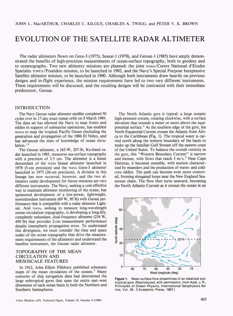
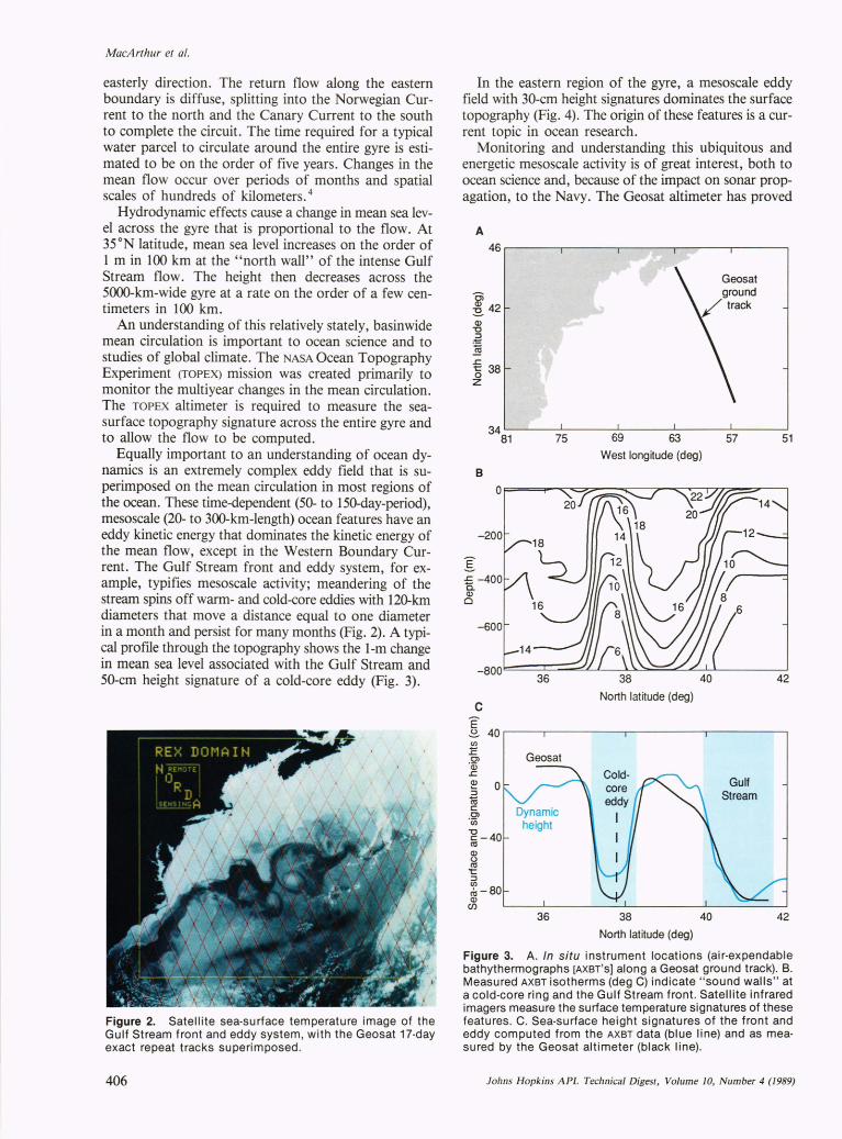
Equally important to an understanding of ocean dy­namics is an extremely complex eddy field that is su­perimposed on the mean circulation in most regions of the ocean. These time-dependent (50- to 150-day-period), mesoscale (20- to 300-km-Iength) ocean features have an eddy kinetic energy that dominates the kinetic energy of the mean flow, except in the Western Boundary Cur­rent. The Gulf Stream front and eddy system, for ex­ample, typifies mesoscale activity; meandering of the stream spins off warm- and cold-core eddies with 120-km diameters that move a distance equal to one diameter in a month and persist for many months (Fig. 2). A typi­cal proflle through the topography shows the I-m change in mean sea level associated with the Gulf Stream and 50-cm height signature of a cold-core eddy (Fig. 3).

Figure 2. Satellite sea-surface temperature image of the Gulf Stream front and eddy system, with the Geosat 17-day exact repeat tracks superimposed.

406

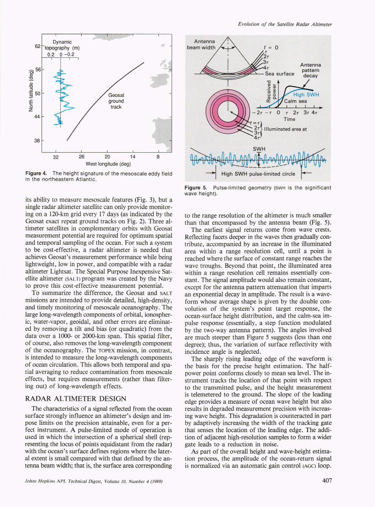
In the eastern region of the gyre, a mesoscale eddy field with 30-cm height signatures dominates the surface topography (Fig. 4). The origin of these features is a cur­rent topic in ocean research.

Monitoring and understanding this ubiquitous and energetic mesoscale activity is of great interest, both to ocean science and, because of the impact on sonar prop­agation, to the Navy. The Geosat altimeter has proved

A 46.------.------.------.--~--._----_.

~ 42 Q) "0 .a N .J::

"§ 38 z

34~~--~------~----~------~----~

81 75 69 63 57 51

B

I a -400 Q)

o

C

E ~ 40 IJ)

E OJ 'm .J:: Q) 0 ::; Ci5 c OJ ·in

"g-40 ~ Q) <.) ~ 't: :::J IJ)

cO- 8O Q)

(f)

West longitude (deg)

36 38 40

North latitude (deg)

Geosat

36 38 40

North latitude (deg)

Gulf Stream

42

42

Figure 3. A. In situ instrument locations (air-expendable bathythermographs [AXBT'S] along a Geosat ground track). B. Measured AXBT isotherms (deg C) indicate "sound walls" at a cold-core ring and the Gulf Stream front. Satellite infrared imagers measure the surface temperature signatures of these features. C. Sea-surface height signatures of the front and eddy computed from the AXBT data (blue line) and as mea­sured by the Geosat altimeter (black line).

fohns Hopkins APL Technical Digest, Volume 10, Number 4 (1989)

Dynamic 62 topography (m)

-56 Ol CD ~ CD "0 ::J

:§ 50 .c 1:: o Z

44

38

0.2 0 -0.2

32 26 20 14 8 West longitude (deg)

Figure 4. The height signature of the mesoscale eddy field in the northeastern Atlantic.

its ability to measure mesoscale features (Fig. 3), but a single radar altimeter satellite can only provide monitor­ing on a 120-km grid every 17 days (as indicated by the Geosat exact repeat ground tracks on Fig. 2). Three al­timeter satellites in complementary orbits with Geosat measurement potential are required for optimum spatial and temporal sampling of the ocean. For such a system to be cost-effective, a radar altimeter is needed that achieves Geosat's measurement performance while being lightweight, low in power, and compatible with a radar altimeter Lightsat. The Special Purpose Inexpensive Sat­ellite altimeter (SALT) program was created by the Navy to prove this cost-effective measurement potential.

To summarize the difference, the Geosat and SALT

missions are intended to provide detailed, high-density, and timely monitoring of mesoscale oceanography. The large long-wavelength components of orbital, ionospher­ic, water-vapor, geoidal, and other errors are eliminat­ed by removing a tilt and bias (or quadratic) from the data over a 1000- or 2000-km span. This spatial filter, of course, also removes the long-wavelength component of the oceanography. The TOPEX mission, in contrast, is intended to measure the long-wavelength components of ocean circulation. This allows both temporal and spa­tial averaging to reduce contamination from mesoscale effects, but requires measurements (rather than filter­ing out) of long-wavelength effects.

RADAR ALTIMETER DESIGN The characteristics of a signal reflected from the ocean

surface strongly influence an altimeter's design and im­pose limits on the precision attainable, even for a per­fect instrument. A pulse-limited mode of operation is used in which the intersection of a spherical shell (rep­resenting the locus of points equidistant from the radar) with the ocean's surface defines regions where the later­al extent is small compared with that defined by the an­tenna beam width; that is, the surface area corresponding

fohns Hopkins APL Technical Digest, Volume 10, Number 4 (1989)

Evolution oj the Satellite Radar Altimeter

t = 0

Antenna pattern decay

- 2r - r 0 r 2r 3r 4r

t=r} Time 2r Illuminated area at 3r 4r

Figure 5. Pulse·limited geometry (SWH is the significant wave height).

to the range resolution of the altimeter is much smaller than that encompassed by the antenna beam (Fig. 5).

The earliest signal returns come from wave crests. Reflecting facets deeper in the waves then gradually con­tribute, accompanied by an increase in the illuminated area within a range resolution cell, until a point is reached where the surface of constant range reaches the wave troughs. Beyond that point, the illuminated area within a range resolution cell remains essentially con­stant. The signal amplitude would also remain constant, except for the antenna pattern attenuation that imparts an exponential decay in amplitude. The result is a wave­form whose average shape is given by the double con­volution of the system's point target response, the ocean-surface height distribution, and the calm-sea im­pulse response (essentially, a step function modulated by the two-way antenna pattern). The angles involved are much steeper than Figure 5 suggests (less than one degree); thus, the variation of surface reflectivity with incidence angle is neglected.

The sharply rising leading edge of the waveform is the basis for the precise height estimation. The half­power point conforms closely to mean sea level. The in­strument tracks the location of that point with respect to the transmitted pulse, and the height measurement is telemetered to the ground. The slope of the leading edge provides a measure of ocean wave height but also results in degraded measurement precision with increas­ing wave height. This degradation is counteracted in part by adaptively increasing the width of the tracking gate that senses the location of the leading edge. The addi­tion of adjacent high-resolution samples to form a wider gate leads to a reduction in noise.

As part of the overall height and wave-height estima­tion process, the amplitude of the ocean-return signal is normalized via an automatic gain control (AGC) loop.

407

MacArthur et al.

Properly calibrated, the AGe setting is a measure of the backscatter coefficient at the surface that, in turn, de­pends on wind speed.

In summary, the altimeter provides three basic mea­surements with precisions specified as follows:

1. Height: less than 3.5 cm for 2-m significant wave height (SWH) (less than 2 cm, including ionospheric cor­rection for TOPEX).

2. Significant wave height: 100/0 of the SWH or 0.5 m, whichever is greater.

3. Wind speed: 1.8 mls over the range of 1 to 18 m/s.

GEOSAT ALTIMETER IMPLEMENTATION The altimeter functions as a 13.5-GHz nadir-looking

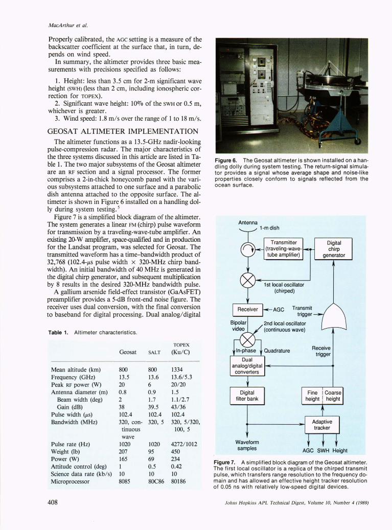
pulse-compression radar. The major characteristics of the three systems discussed in this article are listed in Ta­ble 1. The two major subsystems of the Geosat altimeter are an RF section and a signal processor. The former comprises a 2-in-thick honeycomb panel with the vari­ous subsystems attached to one surface and a parabolic dish antenna attached to the opposite surface. The al­timeter is shown in Figure 6 installed on a handling dol­ly during system testing. 5

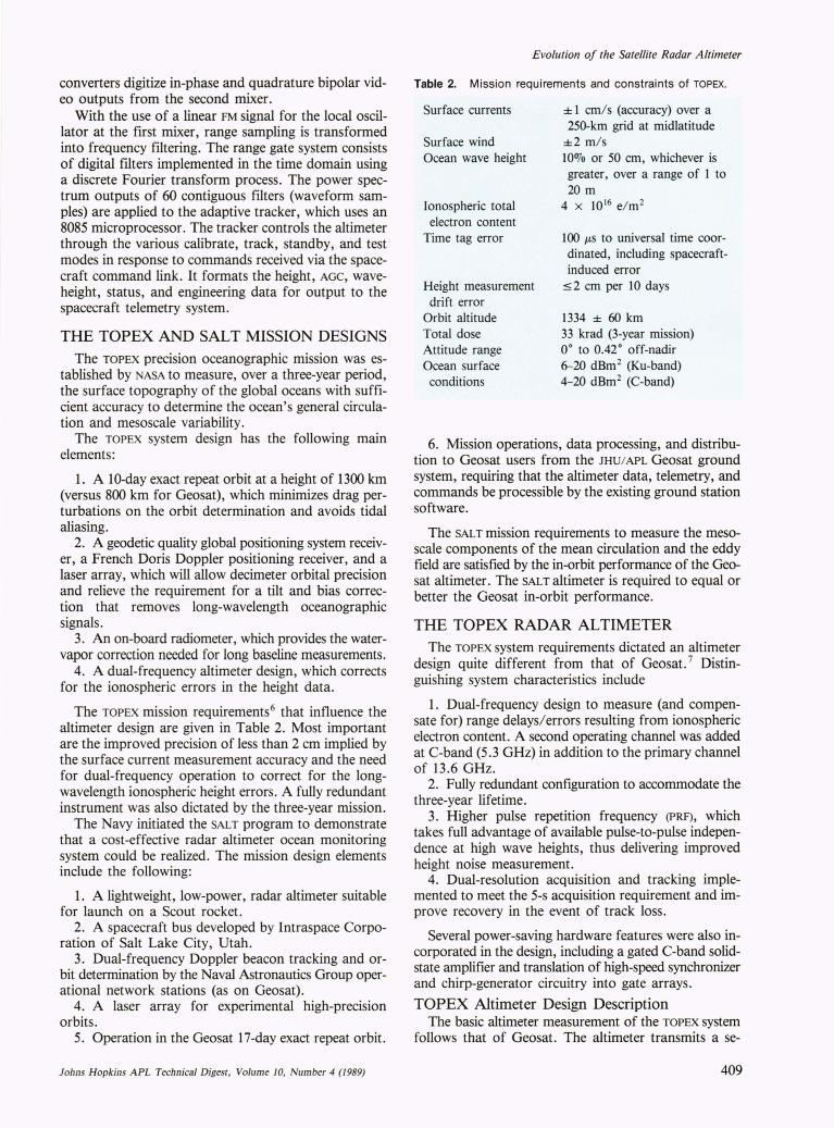
Figure 7 is a simplified block diagram of the altimeter. The system generates a linear FM (chirp) pulse waveform for transmission by a traveling-wave-tube amplifier. An existing ~ W amplifier, space-qualified and in production for the Landsat program, was selected for Geosat. The transmitted waveform has a time-bandwidth product of 32,768 (l02.4-J.ts pulse width x 320-MHz chirp band­width). An initial bandwidth of 40 MHz is generated in the digital chirp generator, and subsequent multiplication by 8 results in the desired 320-MHz bandwidth pulse.

A gallium arsenide field-effect transistor (GaAsFET) preamplifier provides a 5-dB front-end noise figure. The receiver uses dual conversion, with the final conversion to baseband for digital processing. Dual analogi digital

Table 1. Alt imeter characteristics.

Geosat

Mean altitude (km) 800 Frequency (GHz) 13.5 Peak RF power (W) 20 Antenna diameter (m) 0.8

Beam width (deg) 2 Gain (dB) 38

Pulse width CJ.ts) 102.4 Bandwidth (MHz) 320, con-

tinuous wave

Pulse rate (Hz) 1020 Weight (lb) 207 Power (W) 165 Attitude control (deg) 1 Science data rate (kb/s) 10 Microprocessor 8085

408

SALT

800 13.6 6 0.9 1.7 39.5 102.4 320,5

1020 95 69 0.5 10 8OC86

TOPE X

(Ku/e)

1334 13.6/ 5.3 20/20 1.5 1.112.7 43/36 102.4 320, 5/ 320,

100, 5

4272/1012 450 234 0.42 10 80186

Figure 6. The Geosat altimeter is shown installed on a han­dling dolly during system testing. The return-signal simula­tor provides a signal whose average shape and noise-like properties closely conform to signals reflected from the ocean surface.

Antenna

Dual

1-m dish

Transmitter (traveling-wave­tube amplifier)

1 st local oscillator (chirped)

AGC Transmit trigger

2nd local oscillator (continuous wave)

Digital chirp

generator

Receive trigger

analOg/digital ~--------..... converters

Waveform samples AGC SWH Height

Figure 7. A simplified block diagram of the Geosat altimeter. The first local oscillator is a replica of the chirped transmit pulse, which transfers range resolution to the frequency do­main and has allowed an effective height tracker resolution of 0.05 ns with relatively low-speed digital devices.

fohns Hopkins APL Technical Digest, Volume 10, Number 4 (1989)

converters digitize in-phase and quadrature bipolar vid­eo outputs from the second mixer.

With the use of a linear FM signal for the local oscil­lator at the first mixer, range sampling is transformed into frequency filtering. The range gate system consists of digital filters implemented in the time domain using a discrete Fourier transform process. The power spec­trum outputs of 60 contiguous filters (waveform sam­ples) are applied to the adaptive tracker, which uses an 8085 microprocessor. The tracker controls the altimeter through the various calibrate, track, standby, and test modes in response to commands received via the space­craft command link. It formats the height, AGe, wave­height, status, and engineering data for output to the spacecraft telemetry system.

THE TOPEX AND SALT MISSION DESIGNS The TOPEX precision oceanographic mission was es­

tablished by NASA to measure, over a three-year period, the surface topography of the global oceans with suffi­cient accuracy to determine the ocean's general circula­tion and mesoscale variability.

The TOPEX system design has the following main elements:

1. A 10-day exact repeat orbit at a height of 1300 km (versus 800 km for Geosat), which minimizes drag per­turbations on the orbit determination and avoids tidal aliasing.

2. A geodetic quality global positioning system receiv­er, a French Doris Doppler positioning receiver, and a laser array, which will allow decimeter orbital precision and relieve the requirement for a tilt and bias correc­t~on that removes long-wavelength oceanographic SIgnals.

3. An on-board radiometer, which provides the water­vapor correction needed for long baseline measurements.

4. A dual-frequency altimeter design, which corrects for the ionospheric errors in the height data.

The TOPEX mission requirements6 that influence the altimeter design are given in Table 2. Most important are the improved precision of less than 2 cm implied by the surface current measurement accuracy and the need for dual-frequency operation to correct for the long­wavelength ionospheric height errors. A fully redundant instrument was also dictated by the three-year mission.

The Navy initiated the SALT program to demonstrate that a cost-effective radar altimeter ocean monitoring system could be realized. The mission design elements include the following:

1. A lightweight, low-power, radar altimeter suitable for launch on a Scout rocket.

~. A spacecraft bus developed by Intraspace Corpo­ratIOn of Salt Lake City, Utah.

3. Dual-frequency Doppler beacon tracking and or­bit determination by the Naval Astronautics Group oper­ational network stations (as on Geosat).

4. A laser array for experimental high-precision orbits.

5. Operation in the Geosat 17 -day exact repeat orbit.

Johns Hopkins APL Technical Digest, Volume 10, Number 4 (1989)

Evolution of the Satellite Radar Altimeter

Table 2. Mission requirements and constraints of TOPEX.

Surface currents

Surface wind Ocean wave height

Ionospheric total electron content

Time tag error

Height measurement drift error

Orbit altitude Total dose Attitude range Ocean surface conditions

± 1 cmls (accuracy) over a 250-km grid at midlatitude

±2 mls 10070 or 50 cm, whichever is greater, over a range of 1 to 20 m

4 x 10 16 e/ m2

100 J.Ls to universal time coor­dinated, including spacecraft­induced error ~2 cm per 10 days

1334 ± 60 km 33 krad (3-year mission) 0 0 to 0.42 0 off-nadir 6-20 dBm 2 (Ku-band) 4-20 dBm2 (C-band)

6. Mission operations, data processing, and distribu­tion to Geosat users from the JHU/ APL Geosat ground system, requiring that the altimeter data, telemetry, and commands be processible by the existing ground station software.

The SALT mission requirements to measure the meso­scale components of the mean circulation and the eddy field are satisfied by the in-orbit performance of the Geo­sat altimeter. The SALT altimeter is required to equal or better the Geosat in-orbit performance.

THE TOPEX RADAR ALTIMETER The TOPEX system requirements dictated an altimeter

design quite different from that of Geosat. 7 Distin­guishing system characteristics include

1. Dual-frequency design to measure (and compen­sate for) range delays/errors resulting from ionospheric electron content. A second operating channel was added at C-band (5.3 GHz) in addition to the primary channel of 13.6 GHz.

2. Fully redundant configuration to accommodate the three-year lifetime.

3. Higher pulse repetition frequency (PRF), which takes full advantage of available pulse-to-pulse indepen­dence at high wave heights, thus delivering improved height noise measurement.

4. Dual-resolution acquisition and tracking imple­mented to meet the 5-s acquisition requirement and im­prove recovery in the event of track loss.

Several power-saving hardware features were also in­corporated in the design, including a gated C-band solid­state amplifier and translation of high-speed synchronizer and chirp-generator circuitry into gate arrays.

TOPEX Altimeter Design Description The basic altimeter measurement of the TOPEX system

follows that of Geosat. The altimeter transmits a se-

409

MacArthur et al.

quence of linear FM (chirped) pulses to the ocean sur­face. Returned signals reflected from the ocean surface are received by the altimeter's antenna and are then pro­cessed and analyzed to determine time of arrival, details of signal strength, and waveform signature. Series of suc­cessive returns are averaged to yield smoothed data along the satellite subtrack. Additional data processing is per­formed to calculate wave height, spacecraft altitude, al­titude rate, received signal strength, and waveform

Ku-band MTU

Signal processors ~ __ ~

C-band MTU

Chirp generator

samples. A summary of the altimeter's engineering char­acteristics is given in Table 1.

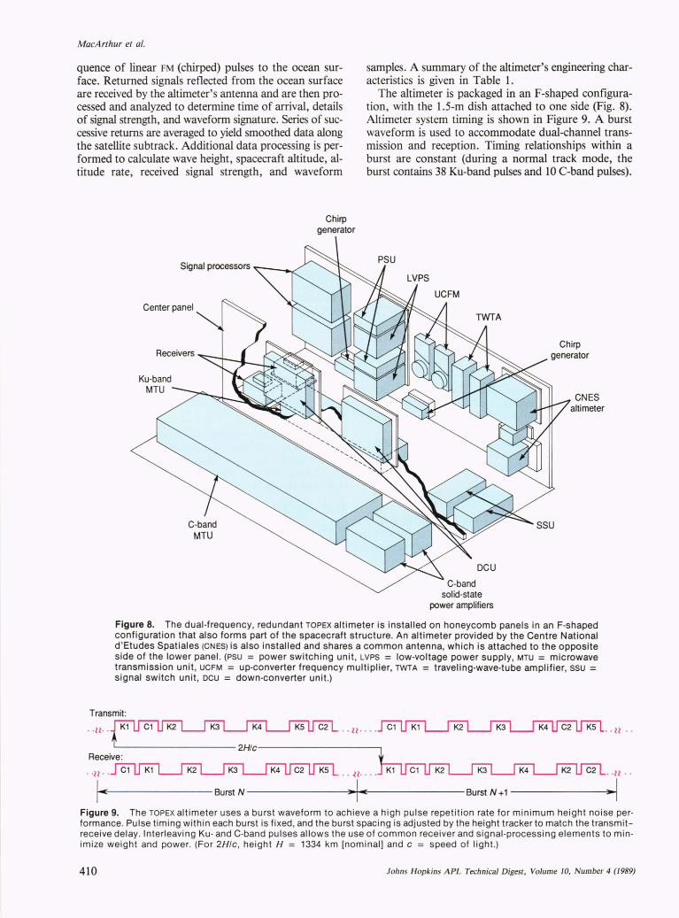
The altimeter is packaged in an F-shaped configura­tion, with the I.S-m dish attached to one side (Fig. 8). Altimeter system timing is shown in Figure 9. A burst waveform is used to accommodate dual-channel trans­mission and reception. Timing relationships within a burst are constant (during a normal track mode, the burst contains 38 Ku-band pulses and 10 C-band pulses).

UCFM

solid-state power amplifiers

Chirp generator

CNES altimeter

Figure 8. The dual-frequency, redundant TOPEX altimeter is installed on honeycomb panels in an F-shaped configuration that also forms part of the spacecraft structure. An altimeter provided by the Centre National d'Etudes Spatiales (CNES) is also installed and shares a common antenna, which is attached to the opposite side of the lower panel. (psu = power switching unit, LVPS = low-voltage power supply, MTU = microwave transmission unit, UCFM = up·converter frequency multiplier, TWTA = traveling-wave-tube amplifier, ssu = signal switch unit, DCU = down·converter unit.)

Transmit:

·· n · . · n ····

~----------------------------------2H/c-------------------.

Receive:

. ' il .. C1 . .. . n . . . . ·il ..

"""I -EE--------- Burst N ----------------~ .. ~lf.oooEE_------------- Burst N + 1 --------------~>-~I Figure 9. The TOPEX altimeter uses a burst waveform to achieve a high pulse repetition rate for minimum height noise per­formance. Pulse timing within each burst is fixed, and the burst spacing is adjusted by the height tracker to match the transmit­receive delay. Interleaving Ku- and C-band pulses allows the use of common receiver and signal-processing elements to min­imize weight and power. (For 2Hlc, height H = 1334 km [nominal] and c = speed of light.)

410 Johns Hopkins APL Technical Digest, Volume 10, Number 4 (1989)

The time interval between the end of the burst and the beginning of the next burst varies to accommodate the range measurement, however. Thus, the average PRF is variable, but the instantaneous (pulse-to-pulse) PRF is fixed.

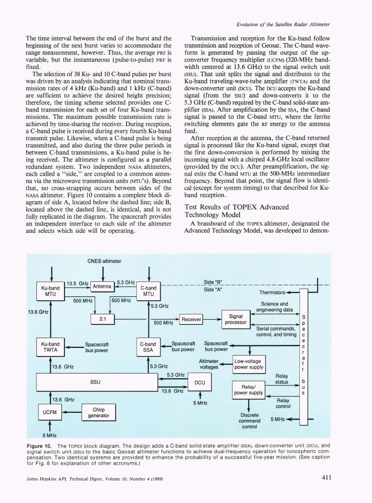
The selection of 38 Ku- and 10 C-band pulses per burst was driven by an analysis indicating that nominal trans­mission rates of 4 kHz (Ku-band) and 1 kHz (C-band) are sufficient to achieve the desired height precision; therefore, the timing scheme selected provides one C­band transmission for each set of four Ku-band trans­missions . The maximum possible transmission rate is achieved by time-sharing the receiver. During reception, a C-band pulse is received during every fourth Ku-band transmit pulse. Likewise, when a C-band pulse is being transmitted, and also during the three pulse periods in between C-band transmissions, a Ku-band pulse is be­ing received. The altimeter is configured as a parallel redundant system. Two independent NASA altimeters, each called a "side," are coupled to a common anten­na via the microwave transmission units (MTU'S). Beyond that, no cross-strapping occurs between sides of the NASA altimeter. Figure 10 contains a complete block di­agram of side A, located below the dashed line; side B, located above the dashed line, is identical, and is not fully replicated in the diagram. The spacecraft provides an independent interface to each side of the altimeter and selects which side will be operating.

CNES altimeter

Evolution of the Satellite Radar A ltimeter

Transmission and reception for the Ku-band follow transmission and reception of Geosat. The C-band wave­form is generated by passing the output of the up­converter frequency multiplier (UCFM) (320-MHz band­width centered at 13.6 GHz) to the signal switch unit (SSU). That unit splits the signal and distributes to the Ku-band traveling-wave-tube amplifier (TWTA) and the down-converter unit (OCU). The ocu accepts the Ku-band signal (from the ssu) and down-converts it to the 5.3 GHz (C-band) required by the C-band solid-state am­plifier (SSA). After amplification by the SSA, the C-band signal is passed to the C-band MTU, where the ferrite switching elements gate the RF energy to the antenna feed.

After reception at the antenna, the C-band returned signal is processed like the Ku-band signal, except that the first down-conversion is performed by mixing the incoming signal with a chirped 4.8-GHz local oscillator (provided by the DCU). After preamplification, the sig­nal exits the C-band MTU at the 500-MHz intermediate frequency. Beyond that point, the signal flow is identi­cal (except for system timing) to that described for Ku­band reception.

Test Results of TOPEX Advanced Technology Model

A brassboard of the TOPEX altimeter, designated the Advanced Technology Model, was developed to demon-

r---L--. _______ ...§~e~B~ ______________ _ Ku-band

MTU

13.6 GHz

Ku-band TWTA

5MHz

.... __ Spacecraft bus power

..... ---; C-band MTU

5.3 GHz

500 MHz

Side "A" Thermistors

Science and engineering data

Signal S processor p

Serial commands, a control, and timing c

Spacecraft e

bus power c r

Low-voltage a

power supply f

Relay status b

Relay/ u power supply s

5MHz Relay control

Discrete command 5MHz

control

Figure 10. The TOPEX block diagram. The design adds a C-band solid-state amplifier (SSA), down-converter un it (DCU), and signal switch unit (SSU) to the basic Geosat altimeter functions to achieve dual-frequency operation for ionospheric com­pensation. Two identical systems are provided to enhance the probability of a successful five-year miss ion . (See capt ion for Fig. 8 for explanation of other acronyms.)

Johns Hopkins A PL Technical Digest, Volume 10, N umber 4 (1989) 411

MacArthur et al.

strate the feasibility of achieving 2-cm measurement pre­cision despite ionospheric propagation errors. Tests were performed by using a specialized test and simulation sys­tem called the Radar Altimeter System Evaluator, which simulated the dual-frequency returns from the ocean af­ter transmission through the ionosphere. 8 Performance results demonstrated that the required dual-frequency combined height precision was satisfied by the altimeter design (Table 3).

THE SALT RADAR ALTIMETER The SALT will perform the same functions as the

Geosat-l altimeter in a unit that uses half the power and weighs half as much. Incorporation of a signal processor of light weight (compared with Geosat-l) and use of a solid-state transmitter result in the substantial weight and power reductions needed for the mission. These critical advances in subsystem technology are described by Per­schy et al. and von Mehlem and Wallis elsewhere in this issue.

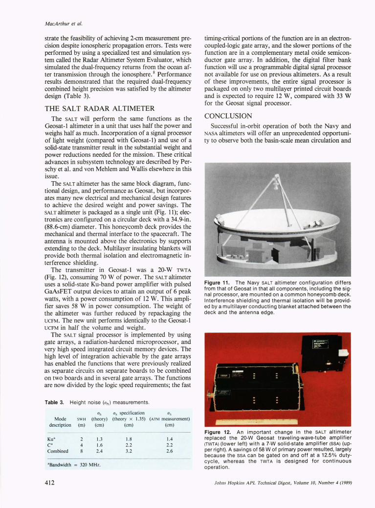
The SALT altimeter has the same block diagram, func­tional design, and performance as Geosat, but incorpor­ates many new electrical and mechanical design features to achieve the desired weight and power savings. The SALT altimeter is packaged as a single unit (Fig. 11); elec­tronics are configured on a circular deck with a 34.9-in. (88.6-cm) diameter. This honeycomb deck provides the mechanical and thermal interface to the spacecraft. The antenna is mounted above the electronics by supports extending to the deck. Multilayer insulating blankets will provide both thermal isolation and electromagnetic in­terference shielding.

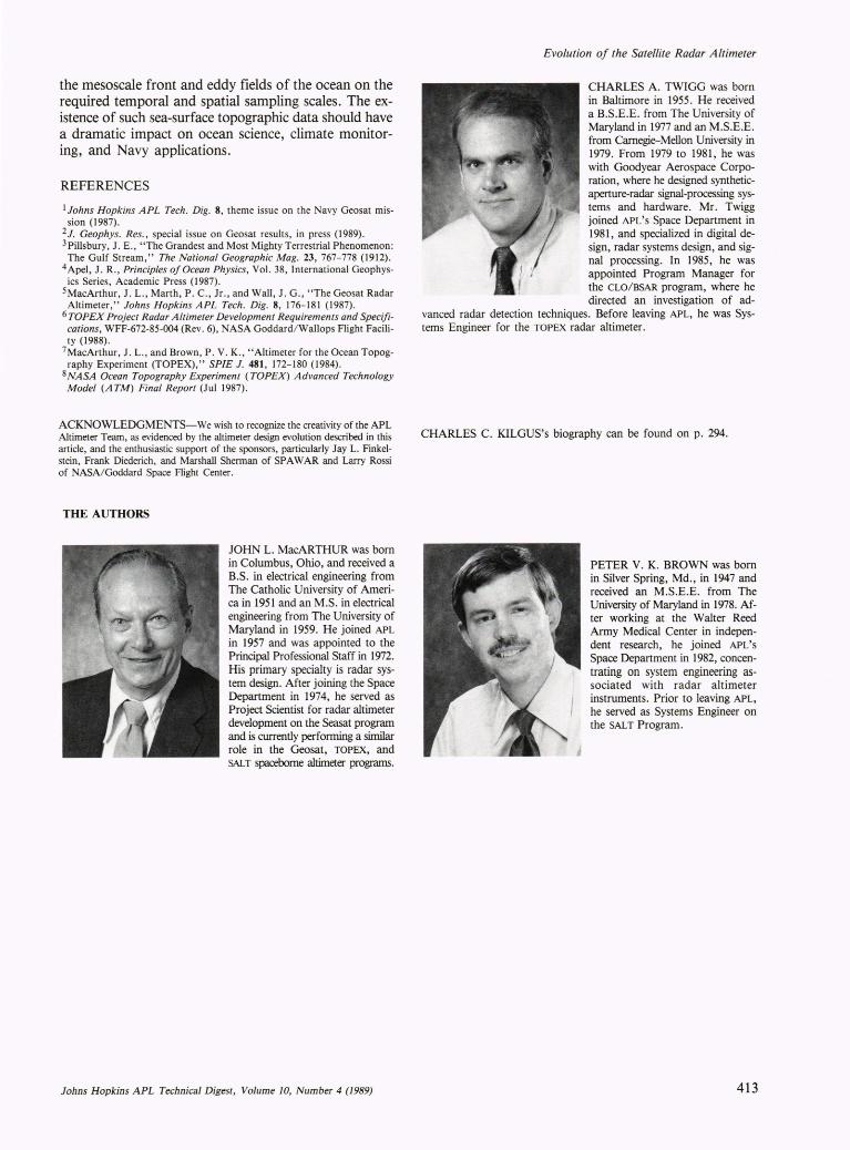
The transmitter in Geosat-l was a 20-W TWTA

(Fig. 12), consuming 70 W of power. The SALT altimeter uses a solid-state Ku-band power amplifier with pulsed GaAsFET output devices to attain an output of 6 peak watts, with a power consumption of 12 W. This ampli­fier saves 58 W in power consumption. The weight of the altimeter was further reduced by repackaging the UCFM. The new unit performs identically to the Geosat-l UCFM in half the volume and weight.

The SALT signal processor is implemented by using gate arrays, a radiation-hardened microprocessor, and very high speed integrated circuit memory devices. The high level of integration achievable by the gate arrays has enabled the functions that were previously realized as separate circuits on separate boards to be combined on two boards and in several gate arrays. The functions are now divided by the logic speed requirements; the fast

Table 3. Height noise (Uh) measurements.

Uh Uh specification Uh

Mode SWH (theory) (theory x 1.35) (A TM measurement) description (m) (cm) (cm) (cm)

Ku 3

C3

Combined

2 4 8

1.3 1.6 2.4

3Bandwidth = 320 MHz.

412

1.8 2.2 3.2

1.4 2.2 2.6

timing-critical portions of the function are in an electron­coupled-logic gate array, and the slower portions of the function are in a complementary metal oxide semicon­ductor gate array. In addition, the digital filter bank function will use a programmable digital signal processor not available for use on previous altimeters. As a result of these improvements, the entire signal processor is packaged on only two multilayer printed circuit boards and is expected to require 12 W, compared with 33 W for the Geosat signal processor.

CONCLUSION Successful in-orbit operation of both the Navy and

NASA altimeters will offer an unprecedented opportuni­ty to observe both the basin-scale mean circulation and

Figure 11. The Navy SALT altimeter configuration differs from that of Geosat in that all components, including the sig­nal processor, are mounted on a common honeycomb deck. Interference shielding and thermal isolation will be provid­ed by a mult ilayer conducting blanket attached between the deck and the antenna edge.

Figure 12. An important change in the SALT altimeter replaced the 20-W Geosat traveling-wave-tube amplifier (TWTA) (lower left) with a 7-W solid-state amplifier (SSA) (up­per right). A savings of 58 W of primary power resulted, largely because the SSA can be gated on and off at a 12.5% duty­cycle, whereas the TWTA is designed for continuous operation.

Johns Hopkins A PL Technical Digest, Volume 10, Number 4 (1989)

the mesoscale front and eddy fields of the ocean on the required temporal and spatial sampling scales. The ex­istence of such sea-surface topographic data should have a dramatic impact on ocean science, climate monitor­ing, and Navy applications.

REFERENCES

I Johns Hopkins APL Tech . Dig. 8, theme issue on the Navy Geosat mis­sion (1987) .

2J. Geophys. Res. , special issue on Geosat results, in press (1989). 3Pillsbury, J . E., " The Grandest and Most Mighty Terrestrial Phenomenon: The Gulf Stream ," The Nalional Geographic Mag. 23,767-778 (1912) .

4Apel, J. R. , Principles of Ocean Physics, Vol. 38, International Geophys­ics Series, Academic Press (1987).

5MacArthur, 1. L., Marth, P . c., Jr., and Wall , J . G., "The Geosat Radar Altimeter," Johns Hopkins APL Tech . Dig. 8, 176-181 (1987) .

6 TOPEX Project Radar Altimeter Development Requirements and Specifi­cations, WFF-672-85-004 (Rev. 6), NASA Goddard/ Wallops Flight Facili­ty (1988).

7MacArthur , J . L. , and Brown, P. V. K., " Altimeter for the Ocean Topog­raphy Experiment (TOPEX), " SPIE J. 481, 172- 180 (1984) .

8 NASA Ocean Topography Experiment (TOPEX) A dvanced Technology Model (ATM) Final Report (Jul 1987).

ACKNOWLEDGMENTS- We wish to recognize the creativity of the APL Altimeter Team, as evidenced by the altimeter design evolution described in this article, and the enthusiastic support of the sponsors, particularly Jay L. Finkel­stein, Frank Diederich, and Marshall Sherman of SPA W AR and Larry Rossi of NASA/ Goddard Space Flight Center.

THE AUTHORS

JOHN L. MacARTHUR was born in Columbus, Ohio, and received a B.S. in electrical engineering from The Catholic University of Ameri­ca in 1951 and an M.S . in electrical engineering from The University of Maryland in 1959. He joined APL in 1957 and was appointed to the Principal Professional Staff in 1972. His primary specialty is radar sys­tem design. After joining the Space Department in 1974, he served as Project Scientist for radar altimeter development on the Seasat program and is currently performing a similar role in the Geosat, TOPEX, and SALT spacebome altimeter programs.

Johns Hopkins APL Technical Digest, Volume 10, Number 4 (1989)

Evolution oj the Satellite Radar Altimeter

CHARLES A. TWIGG was born in Baltimore in 1955. He received a B.S.E.E. from The University of Maryland in 1977 and an M.S.E.E. from Carnegie-Mellon University in 1979. From 1979 to 1981, he was with Goodyear Aerospace Corpo­ration, where he designed synthetic­aperture-radar signal-processing sys­tems and hardware. Mr. Twigg joined APL'S Space Department in 1981, and specialized in digital de­sign, radar systems design, and sig­nal processing. In 1985, he was appointed Program Manager for the CLO/ BSAR program, where he directed an investigation of ad­

vanced radar detection techniques. Before leaving APL, he was Sys­tems Engineer for the TOPEX radar altimeter.

CHARLES C . KILGUS's biography can be found on p. 294.

PETER V. K. BROWN was born in Silver Spring, Md., in 1947 and received an M.S .E.E. from The University of Maryland in 1978. Af­ter working at the Walter Reed Army Medical Center in indepen­dent research, he joined APL's Space Department in 1982, concen­trating on system engineering as­sociated with radar altimeter instruments. Prior to leaving APL, he served as Systems Engineer on the SALT Program.

413