Embed Size (px)
Citation preview
A&A 451, 319–330 (2006)DOI: 10.1051/0004-6361:20054171c© ESO 2006
Astronomy&
Astrophysics
Evolution of magnetic fields and energeticsof flares in active region 8210
S. Régnier1 , and R. C. Canfield2
1 ESA Research and Scientific Support Department, SCI-SH, Keplerlaan 1, 2201 AZ Noordwijk, The Netherlandse-mail: [email protected]
2 Montana State University, Physics Dept., 264 EPS Building, Bozeman, MT 59717, USA
Received 7 September 2005 / Accepted 30 January 2006
ABSTRACT
To better understand eruptive events in the solar corona, we combine sequences of multi-wavelength observations and modelling of the coronalmagnetic field of NOAA AR 8210, a highly flare-productive active region. From the photosphere to the corona, the observations give us infor-mation about the motion of magnetic elements (photospheric magnetograms), the location of flares (e.g., Hα, EUV or soft X-ray brightenings),and the type of events (Hα blueshift events). Assuming that the evolution of the coronal magnetic field above an active region can be describedby successive equilibria, we follow in time the magnetic changes of the 3D nonlinear force-free (nlff) fields reconstructed from a time series ofphotospheric vector magnetograms. We apply this method to AR 8210 observed on May 1, 1998 between 17:00 UT and 21:40 UT. We identifytwo types of horizontal photospheric motions that can drive an eruption: a clockwise rotation of the sunspot, and a fast motion of an emergingpolarity. The reconstructed nlff coronal fields give us a scenario of the confined flares observed in AR 8210: the slow sunspot rotation enablesthe occurence of flare by a reconnection process close to a separatrix surface whereas the fast motion is associated with small-scale recon-nections but no detectable flaring activity. We also study the injection rates of magnetic energy, Poynting flux and relative magnetic helicitythrough the photosphere and into the corona. The injection of magnetic energy by transverse photospheric motions is found to be correlatedwith the storage of energy in the corona and then the release by flaring activity. The magnetic helicity derived from the magnetic field and thevector potential of the nlff configuration is computed in the coronal volume. The magnetic helicity evolution shows that AR 8210 is dominatedby the mutual helicity between the closed and potential fields and not by the self helicity of the closed field which characterizes the twist ofconfined flux bundles. We conclude that for AR 8210 the complex topology is a more important factor than the twist in the eruption process.
Key words. Sun: magnetic fields – Sun: flares – Sun: corona – Sun: evolution
1. Introduction
The structure of the Sun’s corona is dominated by its magneticfield. To understand eruptive events (flares, coronal mass ejec-tions (CMEs) or filament eruptions), we need to know the evo-lution of the 3D magnetic configuration (geometry and topol-ogy) of the corona. In this study, we combine observations ofthe solar atmosphere at various heights with models of the coro-nal magnetic field to determine the sources of flaring activityand the time changes of an active region before and after aflare. We focus our study on a five-hour period which is par-ticularly interesting because (i) it precedes a major flare/CMEevent and (ii) it is well observed with vector magnetograms.
Most flare models (see review by Priest & Forbes 2002;Lin et al. 2003) involve magnetic reconnection processes to ex-plain the rapid conversion of magnetic energy into kinetic en-ergy and thermal energy (hard X-ray sources, soft X-ray flux,
Now at St Andrews University, School of Mathematics, NorthHaugh, St Andrews, Fife KY16 9SS, UK.
brightening in hot EUV lines or in Hα). In the classicalCSHKP model (Carmichael 1964; Sturrock 1968; Hirayama1974; Kopp & Pneuman 1976), the reconnection process oc-curs at the location of an X point in 2D, or at the location of anull point or a separator field line in 3D. In 3D topology (seePriest & Forbes 2000), the reconnection processes involved inflares do not occur only in the vicinity of a null point but canalso be associated with other topological elements (e.g., fansurfaces, spine field lines). The study of the topology of coro-nal magnetic fields should help us to answer important ques-tions for the energetics of flares, including (i) how is magneticenergy stored before the eruption? (ii) Is the stored magneticenergy enough to power a flare or a CME? Question (i) can betackled by following the time evolution of the magnetic energyinjected through the photosphere, and the free magnetic energyavailable in the corona. To answer question (ii), we need tounderstand the temporal and spatial relationship between ob-served brightenings and magnetic field changes in the corona.
Article published by EDP Sciences and available at http://www.edpsciences.org/aa or http://dx.doi.org/10.1051/0004-6361:20054171
320 S. Régnier and R. C. Canfield: AR 8210 evolution
Table 1. Photospheric, chromospheric and coronal observations of AR 8210 on May 1, 1998. ∆x is the pixel size, ∆t is the time between twoconsecutive observations.
Instrument Wavelength Obs. time ∆x ∆t
SOHO/MDI Ni I at 676.8 nm 17:00–23:00 1.′′98 1 min
MSO/IVM FeI at 630.25 nm 17:07–21:40 1.′′1 3 min
NSO/BBSO Hα at 656.3 nm 17:00–21:08 1′′ 1 min
MSO/MCCD ” 17:00–22:00 2.′′4 15 s
SOHO/EIT Fe XII at 19.5 nm 17:00–23:00 2.′′46 15 min
Yohkoh/SXT Soft X-rays 17:16–22:16 4.′′9 and 9.′′8 ∼8 min
The injection of magnetic energy into the corona throughthe photosphere is considered to be associated with thehorizontal displacement of magnetic features on the photo-sphere: emergence (Schmieder et al. 1997; Ishii et al. 1998;Kusano et al. 2002; Nindos & Zhang 2002) and cancellation(Livi et al. 1989; Fletcher et al. 2001) of magnetic flux, rotationof sunspots (Kucera 1982; Lin & Chen 1989; Nightingale et al.2002), and moving magnetic features (Zhang & Wang 2001;Moon et al. 2002). The velocity fields can be detrmined usingthe white light images (Nightingale et al. 2002) or by estimat-ing the small displacements from a Local Correlation Tracking(LCT) technique (November & Simon 1988). Recently sev-eral more powerful techniques have been developed to retrievethe full photospheric velocity field from vector magnetograms(Welsch et al. 2004; Longcope 2004; Georgoulis & LaBonte2006).
In our study, the coronal magnetic field is assumed to bein a force-free equilibrium state at the time of observation.Therefore if the photospheric distribution of vertical electriccurrent density is known in addition to the vertical magneticfield (Sakurai 1982), the nonlinear force-free field (nlff) can beextrapolated in the corona (e.g., Mikic & McClymont 1994;Amari et al. 1997; Wheatland et al. 2000; Yan & Sakurai 2000;Wiegelmann 2004). Inside nlffmagnetic configurations, a morerealistic distribution of twist and shear can be considered incomparison to other assumptions commonly used to extrap-olate the coronal magnetic field (potential, linear force-freefields). These nlff extrapolation methods were applied to solaractive regions using one snapshot of the magnetic field (e.g.,Yan & Wang 1995; Régnier et al. 2002; Bleybel et al. 2002;Régnier & Amari 2004). Here we propose to study the timeevolution of an active region considering that it can be de-scribed by succesive nonlinear force-free equilibria. This as-sumption is justified by considering that the evolution of theactive region is sufficiently slow which means that the pho-tospheric velocities of the footpoints are small compared tocharacteristic speeds in the corona, such as the Alfvén velocity(Antiochos 1987).
Using the above methods to estimate the velocity fields onthe photosphere and the 3D coronal magnetic field, we can es-timate the rate of magnetic energy injected into the corona byphotospheric motions and where this energy is deposited or re-leased in the corona. We can also derive the magnetic helicityand its evolution to understand the effects of reconnection onthe connectivity of field lines. In this work, we have selected
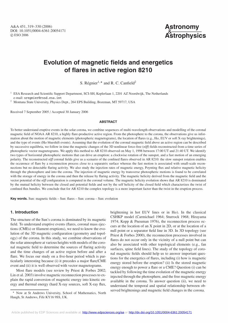
Fig. 1. X-ray flux measured by GOES-8 in the wavelength range0.05−0.4 nm. Gray areas are the flaring periods. The rise (resp. de-cay) phase of flares are the dark (resp. light) gray areas as defined inSect. 3.1.
the active region 8210 (AR 8210) observed on May 1, 1998between 17:00 UT and 21:40 UT for which we have a goodset of data covering the photosphere, the chromosphere andthe corona as well as a high-cadence vector magnetic fieldobservations of good quality. AR 8210 is a well studied ac-tive region for its flaring activity on May 1st and May 2nd(Thompson et al. 2000; Warmuth et al. 2000; Pohjolainen et al.2001; Sterling & Moore 2001a,b; Xia et al. 2001; Sterling et al.2001; Wang et al. 2002). We focus our attention on the timeperiod shown in Fig. 1 by the evolution of the X-ray flux. Wefirst give an overview of the AR 8210 data (see Sect. 2) weuse to analyse the precursors or signatures of flaring activity(Sect. 3): X-ray flux, Hα blueshift events (BSEs), photosphericvelocity fields. In Sect. 4, we describe how to determine andanalyse the 3D magnetic field of AR 8210. We then give a sce-nario of the magnetic field evolution during the flaring period(Sect. 5). The magnetic energy and helicity budgets are derivedin Sects. 6 and 7. In Sect. 8, we discuss the implications ofthose processes for flaring activity and solar eruptions.
2. Data
In Table 1, we summarize the observations on May 1, 1998we are using in this study. Between 17:00 UT and 23:00 UT,we have photospheric line-of-sight and vector magnetograms,
S. Régnier and R. C. Canfield: AR 8210 evolution 321
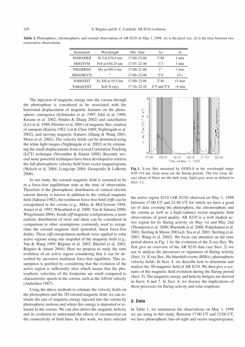
Fig. 2. Images of AR8210: magnetic field (top left), Hα (top right), FeXII at 19.5 nm (bottom left) and soft X-ray (bottom right) images. Welabel characteristic polarities on the SOHO/MDI magnetogram (see Sect. 2.1). The strength of Bz ranges from −2500 G to 1400 G. We labelthe flare sites (A, B, F) as described in Sect. 3.2. Line segments in lower figures roughly indicate the position of the separatrix surfaces that wededuce directly from the EUV and soft X-ray observations.
chromospheric images and spectra, and coronal images. Thosedata guide the analysis presented in later sections.
2.1. Photospheric magnetic field
SOHO/MDI (Michelson Doppler Imager, Scherrer et al. 1995)measures the line-of-sight magnetic field strength deducedfrom the Zeeman splitting of the Ni I 676.8 nm line. During theperiod of observation, we have 1 min cadence full-disc magne-tograms which allow us to study the dynamics of photosphericmagnetic features. The measurement uncertainty is ∼20 G. InFig. 2 top left, we have the distribution of the longitudinalmagnetic field at 20:10 UT in a field-of-view of 600′′ × 600′′.Basically AR 8210 is a sunspot complex of negative polarity
(polarity N1) surrounded by positive polarities (P1–4).AR 8210 also includes parasitic polarities such as N2, whichis a new emerged and moving negative polarity.
IVM at MSO (Imaging Vector Magnetograph/Mees SolarObservatory, Mickey et al. 1996) is a vector magnetographmeasuring the full Stokes profiles of the Fe I 630.25 nm line.The four Stokes parameters, I = (I,Q,U,V), are measuredinside a field-of-view of 256 × 256 pixels with a pixel sizeof 1.1′′ square. The vector magnetograms are built with a seriesof 30 polarisation images obtained over 3 min (Mickey et al.1996). To increase the signal-to-noise ratio and to suppress theeffects of photospheric oscillations, we average the Stokes pro-files over 15 min. In the reduction process, we take into accountthe cross-talk between the I and V profiles as well as scattered
322 S. Régnier and R. C. Canfield: AR 8210 evolution
Fig. 3. Unsigned magnetic flux for the IVM time series and the asso-ciated errors (unit of 1022 G cm2). Gray areas are the flaring periods asdefined in Fig. 1.
light using daily off-limb measurements. A detailed reductionscheme is given by LaBonte et al. (1999). To infer the mag-netic field, the inversion code follows the radiative transfer ofline profiles as in Landolfi & Degl’innocenti (1982) based onUnno (1956) equations and including magneto-optical effects.We then obtain the magnetic field: Blos along the line-of-sight,Btrans and χ the strength and the azimuthal angle of the trans-verse components (in the plane perpendicular to the line-of-sight). We perform the transformation into the disc-center heli-ographic system of coordinates and resolve the 180 ambiguityexisting on the transverse field following Canfield et al. (1993).The resulting magnetic field in a Cartesian frame is (Bx, By, Bz).
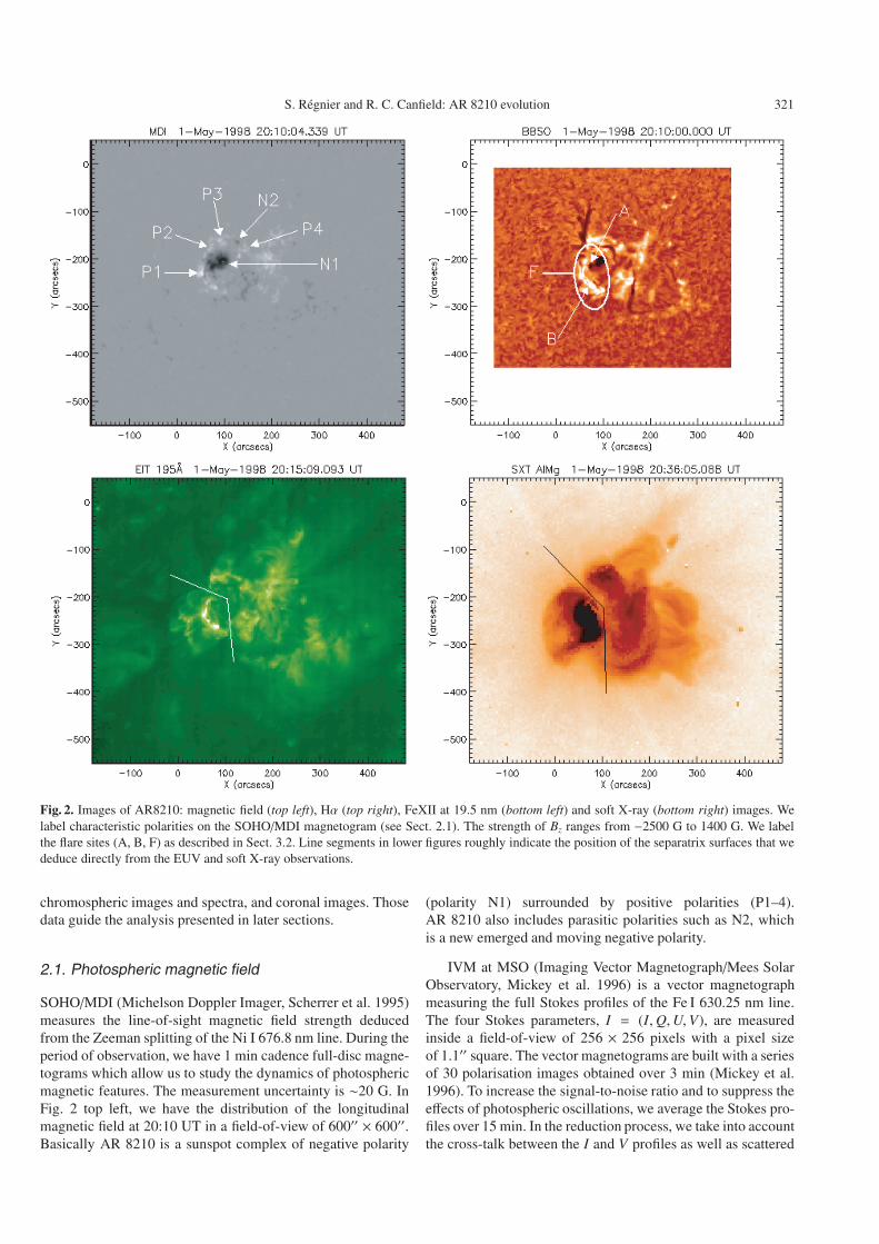
We have performed an analysis of the noise level for thevertical and the transverse components of the magnetic fieldon each of the 15 averaged magnetograms. We proceed as fol-lows: for the vertical magnetic field we plot the distributionwhich can be fitted with a Gaussian profile, for the transversefield we fit the distribution with a χ2 distribution. In both cases,the estimated error is defined as the 3σ value associated withthe width (σ) of the fitted distribution (see Leka & Skumanich1999; Leka 1999). In Fig. 3, we plot the time evolution of thephotospheric unsigned magnetic flux as well as the associatederrors (from the 3σ errors on the Bz component) to show thequality of the data. The estimated formal errors on Bz rangebetween 25 and 50 G. We observe that the variation of themagnetic flux does not exceed 10% and the errors are of 2%of the total flux. The estimated errors on the transverse com-ponents range between 40 and 90 G. By averaging the vectormagnetograms over 15 min, we reduce significantly the noise.For a single magnetogram, the formal errors are ∼150 G orgreater (see e.g. Leka & Skumanich 1999). The net magneticflux which characterizes the imbalance of positive and negativeflux is less than 15% for the IVM data, with an excess of nega-tive flux. For the computation of the nonlinear force-free equi-libria we do not take into account pixels below the estimatederrors on the vertical and transverse components. Therefore thearea that we consider for the computation is different from onetime to another. In Fig. 4, we plot Bz in the IVM field-of-view(background image) for AR 8210 as well as the black contour
Fig. 4. Areas inside the black contour for which the vertical compo-nent and the transverse components are above the thresholds [Bz, Bt]:at 17:13 UT (left) with a threshold of [25 G, 46 G], at 18:01 UT (cen-ter) with a threshold of [30 G, 90 G], and at 21:29 UT (right) with athreshold of [55 G, 75 G].
representating the area of pixels used for the computationfor 3 examples: typical thresholds (left), large threshold valuein the transverse components (center) and large threshold valuein the vertical component (right). As shown in Fig. 4, the areaof valid pixels is enclosed in the black contour and the variationof area from one time to another is not significant.
2.2. Chromospheric data
We use a time series of Big Bear Solar Observatory Hα imagesto observe the reponse of the chromosphere to flaring activi-ties of AR 8210 and its surroundings. Each image observed ev-ery 1 min has a field-of-view of ∼7′ ×7′ with a pixel size of 1′′.In Fig. 2 top right observed on may 1, 1998 at 20:10 UT, weobserved strong absorption features such as the sunspot and fil-aments in the neighborhood of the active region, and bright re-gions (plages) associated with weak magnetic field areas of theactive region.In this Hα image, we label the flare sites: A (Eastpart of the sunspot), B (South-East positive polarity) and F(large area including A and B). The flare sites are identifiedby strong intensity enhancement in the BBSO images and/orby emission profiles as observed in the MCCD data.
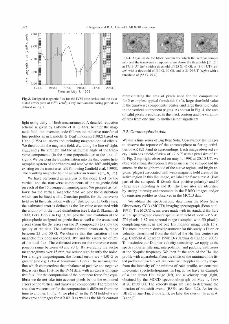
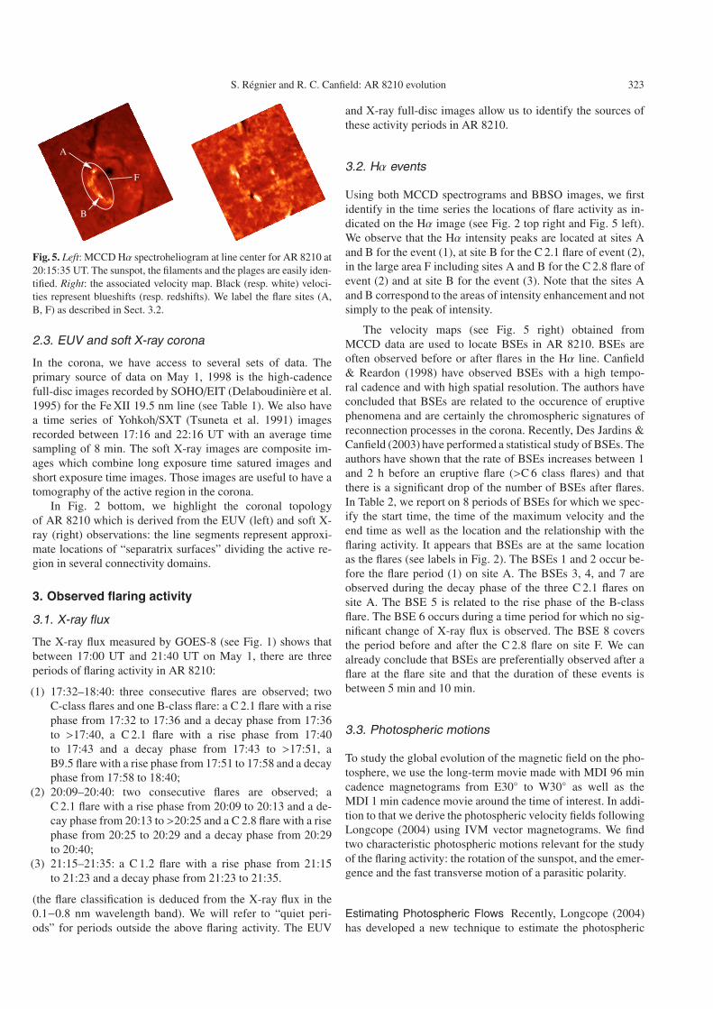
We obtain Hα spectroscopic data from the Mees SolarObservatory CCD (MCCD) imaging spectrograph (Penn et al.1991). The MCCD scans were made with its standard Hα flaresetup: spectrograph camera spatial scan field of view ∼3′ × 4′,2.′′4 pixels, 1.87 nm spectral range (sampled with 50 pixels),completing one scan and one Hα monitor image each 15 s.The most important derived parameter for this study is Dopplervelocity, determined from the shift of the Hα line center (seee.g. Canfield & Reardon 1998; Des Jardins & Canfield 2003).To maximize our Doppler-velocity sensitivity, we apply to thespectra Fourier filtering, interpolation, and padding with zerosat the Nyquist frequency. We then fit the core of the Hα lineprofile with a parabola. From the shifts of the minima of the fit-ted profiles of each pixel, we construct Doppler velocity maps;from the intensity of the minima of each profile, we constructline-center spectroheliograms. In Fig. 5, we have an exampleof a line center Hα image (left) and a velocity map (right)obtained by the MCCD spectroheliograph on May 1, 1998at 20:15:35 UT. The velocity maps are used to determine thelocation of blueshift events (BSEs, see Sect. 3.2). As for theBBSO image (Fig. 2 top right), we label the sites of flares as A,B and F.
S. Régnier and R. C. Canfield: AR 8210 evolution 323
A
B
F
Fig. 5. Left: MCCD Hα spectroheliogram at line center for AR 8210 at20:15:35 UT. The sunspot, the filaments and the plages are easily iden-tified. Right: the associated velocity map. Black (resp. white) veloci-ties represent blueshifts (resp. redshifts). We label the flare sites (A,B, F) as described in Sect. 3.2.
2.3. EUV and soft X-ray corona
In the corona, we have access to several sets of data. Theprimary source of data on May 1, 1998 is the high-cadencefull-disc images recorded by SOHO/EIT (Delaboudinière et al.1995) for the Fe XII 19.5 nm line (see Table 1). We also havea time series of Yohkoh/SXT (Tsuneta et al. 1991) imagesrecorded between 17:16 and 22:16 UT with an average timesampling of 8 min. The soft X-ray images are composite im-ages which combine long exposure time satured images andshort exposure time images. Those images are useful to have atomography of the active region in the corona.
In Fig. 2 bottom, we highlight the coronal topologyof AR 8210 which is derived from the EUV (left) and soft X-ray (right) observations: the line segments represent approxi-mate locations of “separatrix surfaces” dividing the active re-gion in several connectivity domains.
3. Observed flaring activity
3.1. X-ray flux
The X-ray flux measured by GOES-8 (see Fig. 1) shows thatbetween 17:00 UT and 21:40 UT on May 1, there are threeperiods of flaring activity in AR 8210:
(1) 17:32–18:40: three consecutive flares are observed; twoC-class flares and one B-class flare: a C 2.1 flare with a risephase from 17:32 to 17:36 and a decay phase from 17:36to >17:40, a C 2.1 flare with a rise phase from 17:40to 17:43 and a decay phase from 17:43 to >17:51, aB9.5 flare with a rise phase from 17:51 to 17:58 and a decayphase from 17:58 to 18:40;
(2) 20:09–20:40: two consecutive flares are observed; aC 2.1 flare with a rise phase from 20:09 to 20:13 and a de-cay phase from 20:13 to >20:25 and a C 2.8 flare with a risephase from 20:25 to 20:29 and a decay phase from 20:29to 20:40;
(3) 21:15–21:35: a C 1.2 flare with a rise phase from 21:15to 21:23 and a decay phase from 21:23 to 21:35.
(the flare classification is deduced from the X-ray flux in the0.1−0.8 nm wavelength band). We will refer to “quiet peri-ods” for periods outside the above flaring activity. The EUV
and X-ray full-disc images allow us to identify the sources ofthese activity periods in AR 8210.
3.2. Hα events
Using both MCCD spectrograms and BBSO images, we firstidentify in the time series the locations of flare activity as in-dicated on the Hα image (see Fig. 2 top right and Fig. 5 left).We observe that the Hα intensity peaks are located at sites Aand B for the event (1), at site B for the C 2.1 flare of event (2),in the large area F including sites A and B for the C 2.8 flare ofevent (2) and at site B for the event (3). Note that the sites Aand B correspond to the areas of intensity enhancement and notsimply to the peak of intensity.
The velocity maps (see Fig. 5 right) obtained fromMCCD data are used to locate BSEs in AR 8210. BSEs areoften observed before or after flares in the Hα line. Canfield& Reardon (1998) have observed BSEs with a high tempo-ral cadence and with high spatial resolution. The authors haveconcluded that BSEs are related to the occurence of eruptivephenomena and are certainly the chromospheric signatures ofreconnection processes in the corona. Recently, Des Jardins &Canfield (2003) have performed a statistical study of BSEs. Theauthors have shown that the rate of BSEs increases between 1and 2 h before an eruptive flare (>C 6 class flares) and thatthere is a significant drop of the number of BSEs after flares.In Table 2, we report on 8 periods of BSEs for which we spec-ify the start time, the time of the maximum velocity and theend time as well as the location and the relationship with theflaring activity. It appears that BSEs are at the same locationas the flares (see labels in Fig. 2). The BSEs 1 and 2 occur be-fore the flare period (1) on site A. The BSEs 3, 4, and 7 areobserved during the decay phase of the three C 2.1 flares onsite A. The BSE 5 is related to the rise phase of the B-classflare. The BSE 6 occurs during a time period for which no sig-nificant change of X-ray flux is observed. The BSE 8 coversthe period before and after the C 2.8 flare on site F. We canalready conclude that BSEs are preferentially observed after aflare at the flare site and that the duration of these events isbetween 5 min and 10 min.
3.3. Photospheric motions
To study the global evolution of the magnetic field on the pho-tosphere, we use the long-term movie made with MDI 96 mincadence magnetograms from E30 to W30 as well as theMDI 1 min cadence movie around the time of interest. In addi-tion to that we derive the photospheric velocity fields followingLongcope (2004) using IVM vector magnetograms. We findtwo characteristic photospheric motions relevant for the studyof the flaring activity: the rotation of the sunspot, and the emer-gence and the fast transverse motion of a parasitic polarity.
Estimating Photospheric Flows Recently, Longcope (2004)has developed a new technique to estimate the photospheric
324 S. Régnier and R. C. Canfield: AR 8210 evolution
Table 2. List of blueshift events (BSE) observed in AR 8210 from MCCD Hα observations. The flare locations (A, B and F) are describedin Fig. 5.
BSE Start Maximum End Loc. Comments
1 17:07:27 17:09:02 17:10:53 A before event (1)
2 17:18:46 17:19:48 17:21:54 " before event (1)
3 17:35:54 17:38:32 17:40:54 " decay phase of C 2.1 at 17:31
4 17:44:04 17:46:58 17:49:20 " decay phase of C 2.1 at 17:38
5 17:49:20 17:53:49 17:56:43 B impulsive phase of B9.5
6 19:30:10 19:33:51 19:37:32 "
7 20:11:18 20:16:50 20:17:50 " decay phase of C 2.1 at 20:10
8 ∼20:28 ∼20:38 F C 2.8 flare
velocity flow. The minimum energy fit (MEF) method is basedon the vertical component of the ideal induction equation:
∇t · (vzBt − Bzut) =∂Bz
∂t· (1)
To solve this equation, the knowledge of the full photosphericmagnetic vector provided by vector magnetograph such as IVMis needed. By minimizing a functional which resembles the ki-netic energy, the vertical flow field is first derived and then thetransverse velocity field on the photosphere. Longcope (2004)has tested the consistency of this technique with theoreticalcases and also with solar observations. We apply this methodto follow the displacement of magnetic structures in AR 8210,labeled in Fig. 2 top left.
Rotation of Sunspot From the long-term evolution ofAR 8210, we note that the main negative polarity (N1) is slowlyrotating clockwise about its center. The effects of this rotationare most important in the South-East part of AR 8210 where apositive polarity (P1) is moving counter-clockwise around N1.These photospheric motions tend to increase the shear betweenthe sunspot and the positive polarity. The transverse motionsdue to the sunspot rotation are not detected because the uncer-tainty of their measurement (at ∼15 min time intervals) is large(the rotation of the sunspot is just few degrees per hour, see e.g.Brown et al. 2003).
Emerging Flux An other interesting photospheric motion isthe emergence of a parasitic polarity (N2) associated with hightransverse velocity field toward the South-West. We measure atransverse velocity of ∼0.7 km s−1. The increase of magneticflux is estimated to be ∼33% in 4 h. The emergence of flux isa precursor of eruption in active region. Therefore we need tostudy the time evolution of this polarity to understand the dis-turbances created by its emergence inside a pre-existing mag-netic configuration. Note that to compute the magnetic fluxassociated with the polarity N2, we have extracted a squareof 30 × 30 pixels of the cross-correlated time series of vectormagnetograms only including negative values of Bz from N2.
In AR 8210, we have observed numerous flares, blueshiftevents associated with reconnection, and photospheric mo-tions. In the following, we combine those three signatures of
eruptions and the time evolution of the nonlinear force-freemagnetic configurations to give a scenario of the flare process.
4. 3D coronal magnetic configurations
4.1. Electric current density and α distribution
From the three components of the photospheric magnetic field(Bx,phot, By,phot, Bz,phot), we can derive the distribution of theelectric current density, Jz,phot and the distribution of the force-free function, αphot as follows:
Jz,phot =1µ0
(∂By,phot
∂x− ∂Bx,phot
∂y
)(2)
and
αphot =µ0 Jz,phot
Bz,phot
=1
Bz,phot
(∂By,phot
∂x− ∂Bx,phot
∂y
)· (3)
We first analyse the distributions of αphot which is computedfor the magnetic field strength over the thresholds defined inSect. 2.1. We study the time evolution of the mean α value aswell as the width of the distribution at 3σ between 17:00 UTand 21:40 UT (see Sect. 2.1) computed following Leka &Skumanich (1999). We note that the mean values of α are pos-itive and less than 10−2 Mm−1. The α value is almost constantduring the time evolution. The dispersion is between −7× 10⁻²
and 7 × 10⁻² Mm−1. According to Régnier (2001) and Régnier& Amari (2004), α often ranges between −1 and +1 Mm−1
with α values of ±0.1 Mm−1 for twisted flux tubes. Thereforethe α value and its dispersion indicate that there is only a smallamount of twist in AR 8210.
In order to describe the coronal field as a nonlinear force-free equilibrium, there are several requirements on the prop-erties of the current density distribution, Jz,phot. The electriccurrent should be balanced: the total electric current should bezero. The positive currents from one polarity should be equal tothe negative currents in the opposite polarity. These propertiescan be written as follows:∫Σ+
Jz,phot dS =∫Σ−
Jz,phot dS , (4)
S. Régnier and R. C. Canfield: AR 8210 evolution 325
and∫Σ+
|J±z,phot| dS =∫Σ−|J∓z,phot| dS , (5)
and consequently,∫Σ±
Jz,phot dS = 0 (6)
where Σ+ (resp. Σ−) is where Bz,phot > 0 (resp. Bz,phot < 0)and J±z,phot is only considered where Jz,phot is positive or negativerespectively.
As an example, we study the distributions for the IVM vec-tor magnetogram at 17:13 UT. The thresholds on the magneticfield components are 25 G for Bz and 46 G for Bt. The ratio ofthe area of strong field region to the area of weak field region isabout 1.2. The electric current imbalance (from Eq. (4)) is 8%and from Eq. (5) the electric current imbalance is 30%.
The imbalance of electric current is plausibly due to thefact that the current in the strong-field regions is detected be-cause the observed fields there exceed the threshold requiredfor Jz calculations while that in weak-field regions is not de-tected. Note that the imbalance is negative, as one would ex-pect, since Jz is mostly negative in the sunspot N1 where thefield strength is high and then Jz well estimated.
4.2. nlff reconstruction
To determine the structure of the coronal field we use thenonlinear force-free approximation based on a vector poten-tial Grad-Rubin (1958) method by using the XTRAPOL code(Amari et al. 1997, 1999). The nlff field in the corona is thengoverned by the following equations:
∇ ∧ B = αB, (7)
B · ∇α = 0, (8)
∇ · B = 0, (9)
where B is the magnetic field vector in the domain Ω abovethe photosphere, δΩ, and α is a function of space defined as theratio of the vertical current density, Jz and the vertical magneticfield component, Bz (see Eq. (3)). From Eq. (8), α is constantalong a field line. In terms of the magnetic field B, the Grad-Rubin iterative scheme can be written as follows:
B(n) · ∇α(n) = 0 in Ω, (10)
α(n) |δΩ± = h, (11)
where δΩ± is defined as the domain on the photosphere forwhich Bz is positive (+) or negative (−) and,
∇ ∧ B(n+1) = α(n)B(n) in Ω, (12)
∇ · B(n+1) = 0 in Ω, (13)
B(n+1)z |δΩ = g, (14)
lim|r|→∞
|B| = 0. (15)
The boundary conditions on the photosphere are given by thedistribution, g of Bz on δΩ (see Eq. (14)) and by the distribu-tion h of α on δΩ for a given polarity (see Eq. (11)). We alsoimpose that
Bn = 0 on Σ − δΩ (16)
where Σ is the surface of the computational box, n refers to thenormal component to the surface. These conditions mean thatno field line can enter or leave to computational box, or in otherwords that the studied active region is magnetically isolated.
Practically, the boundary conditions on the photosphereare: the observed vertical component of the magnetic field,Bz,phot in the disc-center heliographic system of coordinatesallowing the computation in cartesian coordinates, and theαphot distribution given by Eq. (3) in a chosen polarity (we havechosen the negative polarity which represents the sunspot N1of the active region). In order to ensure that the entire ac-tive region is included in the field-of-view, we have createdcomposite vector magnetograms by combining IVM magne-tograms (strong-field regions) and MDI magnetograms (sur-rounding weak-field regions). We then compute the nonlinearforce-free field for the time series of composite magnetogramsusing a cross-correlation technique between each magnetogramand a non-uniform grid which reduces the computational time.Those properties insure that we reconstruct the same volume ofthe corona. Therefore we can study the time evolution of rele-vant quantities as the magnetic energy or the relative magnetichelicity.
4.3. Basic topology
An interesting property of a magnetic configuration is given byits skeleton. The skeleton (Priest & Forbes 2000) correspondsto all topological elements inside a 3D magnetic field includ-ing null points, spine field lines, separatrix surfaces and sepa-rators. To analyse the evolution of AR 8210, we determine var-ious topological elements. First we find the null points on thephotosphere by determining where the magnetic field vanishesand corresponds to a local minima and for which the transversecomponents vanish. Around the null point, the magnetic fieldhas three eigenvalues, λi(i = 1, 2, 3), that sum to zero to satisfyEq. (9). An eigenvector is associated with each eigenvalue (notnecessarily three perpendicular vectors). If one eigenvalue ispositive (resp. negative) and the two others are negative (resp.positive), the spine is the isolated field line directed away from(resp. toward) the null and the separatrix surface consists offield lines radiating toward (resp. away from) the null. The sep-aratrix surfaces give us the definition of the different connec-tivity domains that comprise AR 8210.
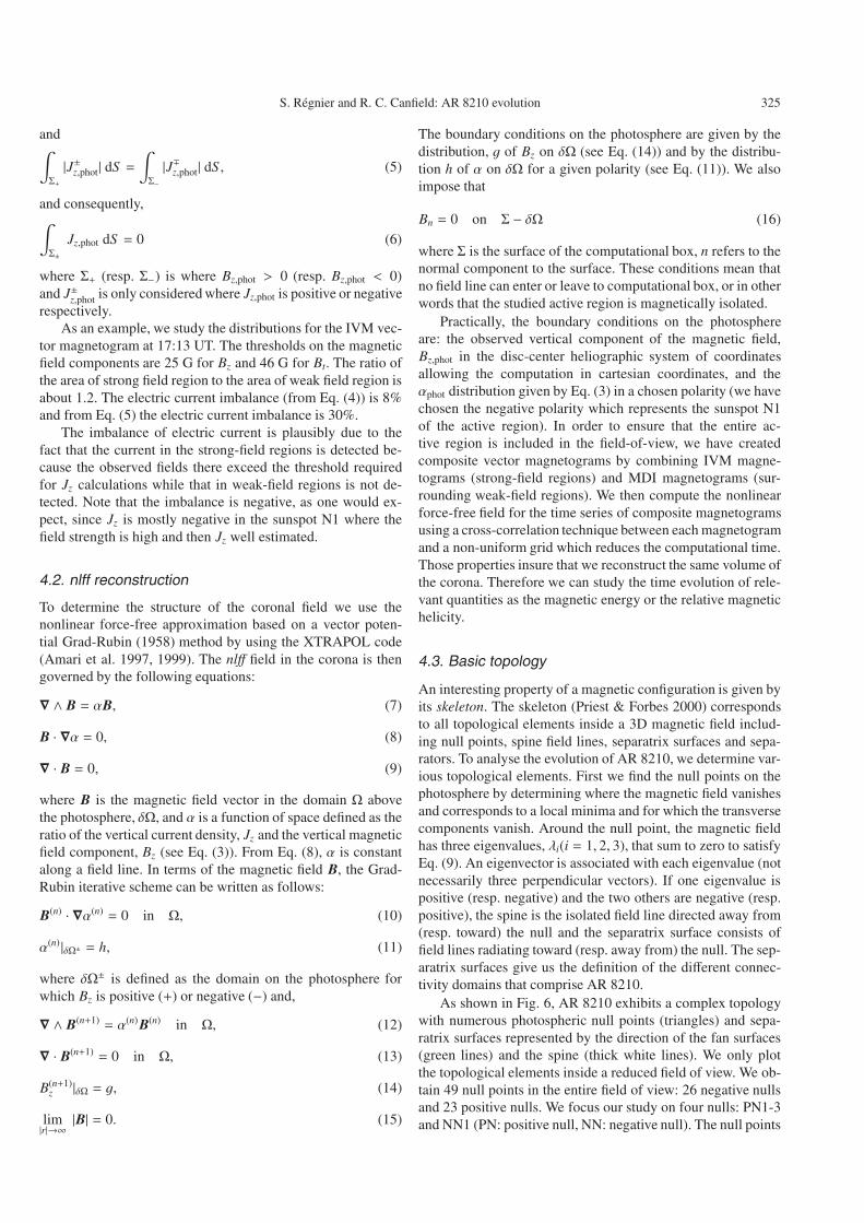
As shown in Fig. 6, AR 8210 exhibits a complex topologywith numerous photospheric null points (triangles) and sepa-ratrix surfaces represented by the direction of the fan surfaces(green lines) and the spine (thick white lines). We only plotthe topological elements inside a reduced field of view. We ob-tain 49 null points in the entire field of view: 26 negative nullsand 23 positive nulls. We focus our study on four nulls: PN1-3and NN1 (PN: positive null, NN: negative null). The null points
326 S. Régnier and R. C. Canfield: AR 8210 evolution
PN1–3 and their associated separatrix surface will be investi-gated in the next section. NN1 has a spine field line connectedwith surrounding negative polarities. The separatrix surface isin the same direction as the South separatrix surface shown onEUV and soft X-ray images (Fig. 2 bottom). The topology doesnot change dramatically during the evolution of AR 8210 (dur-ing the studied time period).
5. Flares, photospheric motions and magneticreconnection
5.1. 3D magnetic evolution associated with precursors
We now analyse the coronal magnetic changes during this timeperiod for the emerging, moving magnetic feature, and the ro-tating sunspot (see Sect. 3.3). We describe small reconnectionprocesses associated with photospheric motions. By “small”reconnections we mean reconnection processes which do notmodify the configuration of the entire active region, but forwhich the connectivity of field lines is modified locally.
5.1.1. Emerging flux
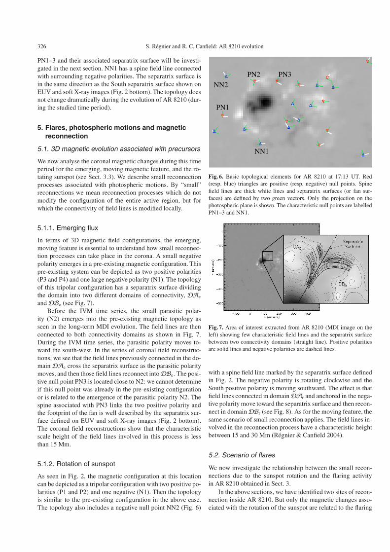
In terms of 3D magnetic field configurations, the emerging,moving feature is essential to understand how small reconnec-tion processes can take place in the corona. A small negativepolarity emerges in a pre-existing magnetic configuration. Thispre-existing system can be depicted as two positive polarities(P3 and P4) and one large negative polarity (N1). The topologyof this tripolar configuration has a separatrix surface dividingthe domain into two different domains of connectivity, DAe
andDBe (see Fig. 7).Before the IVM time series, the small parasitic polar-
ity (N2) emerges into the pre-existing magnetic topology asseen in the long-term MDI evolution. The field lines are thenconnected to both connectivity domains as shown in Fig. 7.During the IVM time series, the parasitic polarity moves to-ward the south-west. In the series of coronal field reconstruc-tions, we see that the field lines previously connected in the do-main DAe cross the separatrix surface as the parasitic polaritymoves, and then those field lines reconnect intoDBe. The posi-tive null point PN3 is located close to N2: we cannot determineif this null point was already in the pre-existing configurationor is related to the emergence of the parasitic polarity N2. Thespine associated with PN3 links the two positive polarity andthe footprint of the fan is well described by the separatrix sur-face defined on EUV and soft X-ray images (Fig. 2 bottom).The coronal field reconstructions show that the characteristicscale height of the field lines involved in this process is lessthan 15 Mm.
5.1.2. Rotation of sunspot
As seen in Fig. 2, the magnetic configuration at this locationcan be depicted as a tripolar configuration with two positive po-larities (P1 and P2) and one negative (N1). Then the topologyis similar to the pre-existing configuration in the above case.The topology also includes a negative null point NN2 (Fig. 6)
NN1
PN1
PN2 PN3
NN2
Fig. 6. Basic topological elements for AR 8210 at 17:13 UT. Red(resp. blue) triangles are positive (resp. negative) null points. Spinefield lines are thick white lines and separatrix surfaces (or fan sur-faces) are defined by two green vectors. Only the projection on thephotospheric plane is shown. The characteristic null points are labelledPN1–3 and NN1.
Fig. 7. Area of interest extracted from AR 8210 (MDI image on theleft) showing few characteristic field lines and the separatrix surfacebetween two connectivity domains (straight line). Positive polaritiesare solid lines and negative polarities are dashed lines.
with a spine field line marked by the separatrix surface definedin Fig. 2. The negative polarity is rotating clockwise and theSouth positive polarity is moving southward. The effect is thatfield lines connected in domainDAr and anchored in the nega-tive polarity move toward the separatrix surface and then recon-nect in domainDBr (see Fig. 8). As for the moving feature, thesame scenario of small reconnection applies. The field lines in-volved in the reconnection process have a characteristic heightbetween 15 and 30 Mm (Régnier & Canfield 2004).
5.2. Scenario of flares
We now investigate the relationship between the small recon-nections due to the sunspot rotation and the flaring activityin AR 8210 obtained in Sect. 3.
In the above sections, we have identified two sites of recon-nection inside AR 8210. But only the magnetic changes asso-ciated with the rotation of the sunspot are related to the flaring
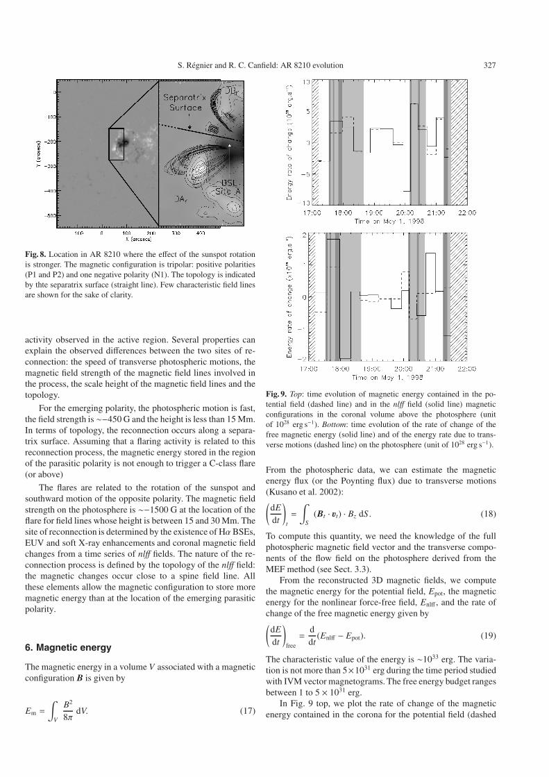
S. Régnier and R. C. Canfield: AR 8210 evolution 327
Fig. 8. Location in AR 8210 where the effect of the sunspot rotationis stronger. The magnetic configuration is tripolar: positive polarities(P1 and P2) and one negative polarity (N1). The topology is indicatedby thte separatrix surface (straight line). Few characteristic field linesare shown for the sake of clarity.
activity observed in the active region. Several properties canexplain the observed differences between the two sites of re-connection: the speed of transverse photospheric motions, themagnetic field strength of the magnetic field lines involved inthe process, the scale height of the magnetic field lines and thetopology.
For the emerging polarity, the photospheric motion is fast,the field strength is ∼−450 G and the height is less than 15 Mm.In terms of topology, the reconnection occurs along a separa-trix surface. Assuming that a flaring activity is related to thisreconnection process, the magnetic energy stored in the regionof the parasitic polarity is not enough to trigger a C-class flare(or above)
The flares are related to the rotation of the sunspot andsouthward motion of the opposite polarity. The magnetic fieldstrength on the photosphere is ∼−1500 G at the location of theflare for field lines whose height is between 15 and 30 Mm. Thesite of reconnection is determined by the existence of HαBSEs,EUV and soft X-ray enhancements and coronal magnetic fieldchanges from a time series of nlff fields. The nature of the re-connection process is defined by the topology of the nlff field:the magnetic changes occur close to a spine field line. Allthese elements allow the magnetic configuration to store moremagnetic energy than at the location of the emerging parasiticpolarity.
6. Magnetic energy
The magnetic energy in a volume V associated with a magneticconfiguration B is given by
Em =
∫V
B2
8πdV. (17)
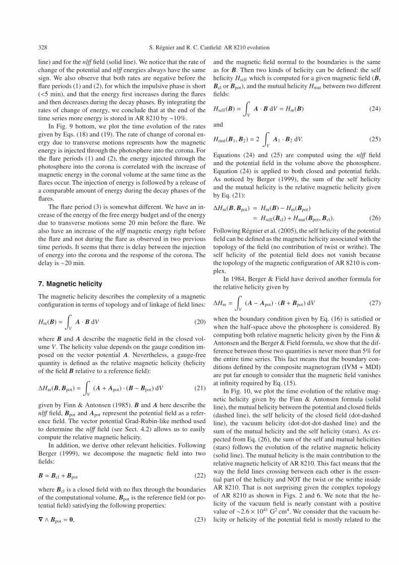
Fig. 9. Top: time evolution of magnetic energy contained in the po-tential field (dashed line) and in the nlff field (solid line) magneticconfigurations in the coronal volume above the photosphere (unitof 1028 erg s−1). Bottom: time evolution of the rate of change of thefree magnetic energy (solid line) and of the energy rate due to trans-verse motions (dashed line) on the photosphere (unit of 1028 erg s−1).
From the photospheric data, we can estimate the magneticenergy flux (or the Poynting flux) due to transverse motions(Kusano et al. 2002):(dEdt
)t
=
∫S
(Bt · ut) · Bz dS . (18)
To compute this quantity, we need the knowledge of the fullphotospheric magnetic field vector and the transverse compo-nents of the flow field on the photosphere derived from theMEF method (see Sect. 3.3).
From the reconstructed 3D magnetic fields, we computethe magnetic energy for the potential field, Epot, the magneticenergy for the nonlinear force-free field, Enlff , and the rate ofchange of the free magnetic energy given by(dEdt
)free
=ddt
(Enlff − Epot). (19)
The characteristic value of the energy is ∼1033 erg. The varia-tion is not more than 5×1031 erg during the time period studiedwith IVM vector magnetograms. The free energy budget rangesbetween 1 to 5 × 1031 erg.
In Fig. 9 top, we plot the rate of change of the magneticenergy contained in the corona for the potential field (dashed
328 S. Régnier and R. C. Canfield: AR 8210 evolution
line) and for the nlff field (solid line). We notice that the rate ofchange of the potential and nlff energies always have the samesign. We also observe that both rates are negative before theflare periods (1) and (2), for which the impulsive phase is short(<5 min), and that the energy first increases during the flaresand then decreases during the decay phases. By integrating therates of change of energy, we conclude that at the end of thetime series more energy is stored in AR 8210 by ∼10%.
In Fig. 9 bottom, we plot the time evolution of the ratesgiven by Eqs. (18) and (19). The rate of change of coronal en-ergy due to transverse motions represents how the magneticenergy is injected through the photosphere into the corona. Forthe flare periods (1) and (2), the energy injected through thephotosphere into the corona is correlated with the increase ofmagnetic energy in the coronal volume at the same time as theflares occur. The injection of energy is followed by a release ofa comparable amount of energy during the decay phases of theflares.
The flare period (3) is somewhat different. We have an in-crease of the energy of the free energy budget and of the energydue to transverse motions some 20 min before the flare. Wealso have an increase of the nlff magnetic energy right beforethe flare and not during the flare as observed in two previoustime periods. It seems that there is delay between the injectionof energy into the corona and the response of the corona. Thedelay is ∼20 min.
7. Magnetic helicity
The magnetic helicity describes the complexity of a magneticconfiguration in terms of topology and of linkage of field lines:
Hm(B) =∫
VA · B dV (20)
where B and A describe the magnetic field in the closed vol-ume V . The helicity value depends on the gauge condition im-posed on the vector potential A. Nevertheless, a gauge-freequantity is defined as the relative magnetic helicity (helicityof the field B relative to a reference field):
∆Hm(B, Bpot) =∫
V(A + Apot) · (B − Bpot) dV (21)
given by Finn & Antonsen (1985). B and A here describe thenlff field, Bpot and Apot represent the potential field as a refer-ence field. The vector potential Grad-Rubin-like method usedto determine the nlff field (see Sect. 4.2) allows us to easilycompute the relative magnetic helicity.
In addition, we derive other relevant helicities. FollowingBerger (1999), we decompose the magnetic field into twofields:
B = Bcl + Bpot (22)
where Bcl is a closed field with no flux through the boundariesof the computational volume, Bpot is the reference field (or po-tential field) satisfying the following properties:
∇ ∧ Bpot = 0, (23)
and the magnetic field normal to the boundaries is the sameas for B. Then two kinds of helicity can be defined: the selfhelicity Hself which is computed for a given magnetic field (B,Bcl or Bpot), and the mutual helicity Hmut between two differentfields:
Hself(B) =∫
VA · B dV = Hm(B) (24)
and
Hmut(B1, B2) = 2∫
VA1 · B2 dV. (25)
Equations (24) and (25) are computed using the nlff fieldand the potential field in the volume above the photosphere.Equation (24) is applied to both closed and potential fields.As noticed by Berger (1999), the sum of the self helicityand the mutual helicity is the relative magnetic helicity givenby Eq. (21):
∆Hm(B, Bpot) = Hm(B) − Hm(Bpot)
= Hself(Bcl) + Hmut(Bpot, Bcl). (26)
Following Régnier et al. (2005), the self helicity of the potentialfield can be defined as the magnetic helicity associated with thetopology of the field (no contribution of twist or writhe). Theself helicity of the potential field does not vanish becausethe topology of the magnetic configuration of AR 8210 is com-plex.
In 1984, Berger & Field have derived another formula forthe relative helicity given by
∆Hm =
∫V
(A − Apot) · (B + Bpot) dV (27)
when the boundary condition given by Eq. (16) is satisfied orwhen the half-space above the photosphere is considered. Bycomputing both relative magnetic helicity given by the Finn &Antonsen and the Berger & Field formula, we show that the dif-ference between those two quantities is never more than 5% forthe entire time series. This fact means that the boundary con-ditions defined by the composite magnetogram (IVM + MDI)are put far enough to consider that the magnetic field vanishesat infinity required by Eq. (15).
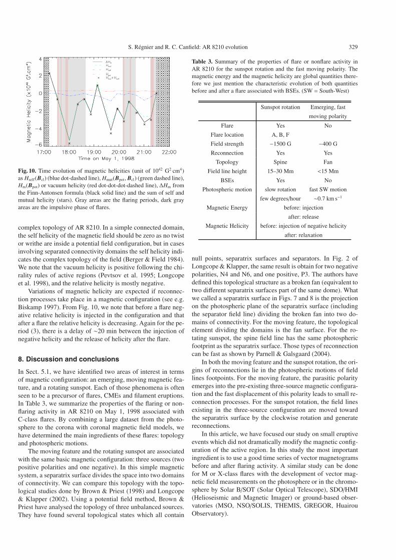
In Fig. 10, we plot the time evolution of the relative mag-netic helicity given by the Finn & Antonsen formula (solidline), the mutual helicity between the potential and closed fields(dashed line), the self helicity of the closed field (dot-dashedline), the vacuum helicity (dot-dot-dot-dashed line) and thesum of the mutual helicity and the self helicity (stars). As ex-pected from Eq. (26), the sum of the self and mutual helicities(stars) follows the evolution of the relative magnetic helicity(solid line). The mutual helicity is the main contribution to therelative magnetic helicity of AR 8210. This fact means that theway the field lines crossing between each other is the essen-tial part of the helicity and NOT the twist or the writhe insideAR 8210. That is not surprising given the complex topologyof AR 8210 as shown in Figs. 2 and 6. We note that the he-licity of the vacuum field is nearly constant with a positivevalue of ∼2.6 × 1041 G2 cm4. We consider that the vacuum he-licity or helicity of the potential field is mostly related to the
S. Régnier and R. C. Canfield: AR 8210 evolution 329
Fig. 10. Time evolution of magnetic helicities (unit of 1042 G2 cm4)as Hself (Bcl) (blue dot-dashed line), Hmut(Bpot, Bcl) (green dashed line),Hm(Bpot) or vacuum helicity (red dot-dot-dot-dashed line), ∆Hm fromthe Finn-Antonsen formula (black solid line) and the sum of self andmutual helicity (stars). Gray areas are the flaring periods, dark grayareas are the impulsive phase of flares.
complex topology of AR 8210. In a simple connected domain,the self helicity of the magnetic field should be zero as no twistor writhe are inside a potential field configuration, but in casesinvolving separated connectivity domains the self helicity indi-cates the complex topology of the field (Berger & Field 1984).We note that the vacuum helicity is positive following the chi-rality rules of active regions (Pevtsov et al. 1995; Longcopeet al. 1998), and the relative helicity is mostly negative.
Variations of magnetic helicity are expected if reconnec-tion processes take place in a magnetic configuration (see e.g.Biskamp 1997). From Fig. 10, we note that before a flare neg-ative relative helicity is injected in the configuration and thatafter a flare the relative helicity is decreasing. Again for the pe-riod (3), there is a delay of ∼20 min between the injection ofnegative helicity and the release of helicity after the flare.
8. Discussion and conclusions
In Sect. 5.1, we have identified two areas of interest in termsof magnetic configuration: an emerging, moving magnetic fea-ture, and a rotating sunspot. Each of those phenomena is oftenseen to be a precursor of flares, CMEs and filament eruptions.In Table 3, we summarize the properties of the flaring or non-flaring activity in AR 8210 on May 1, 1998 associated withC-class flares. By combining a large dataset from the photo-sphere to the corona with coronal magnetic field models, wehave determined the main ingredients of these flares: topologyand photospheric motions.
The moving feature and the rotating sunspot are associatedwith the same basic magnetic configuration: three sources (twopositive polarities and one negative). In this simple magneticsystem, a separatrix surface divides the space into two domainsof connectivity. We can compare this topology with the topo-logical studies done by Brown & Priest (1998) and Longcope& Klapper (2002). Using a potential field method, Brown &Priest have analysed the topology of three unbalanced sources.They have found several topological states which all contain
Table 3. Summary of the properties of flare or nonflare activity inAR 8210 for the sunspot rotation and the fast moving polarity. Themagnetic energy and the magnetic helicity are global quantities there-fore we just mention the characteristic evolution of both quantitiesbefore and after a flare associated with BSEs. (SW = South-West)
Sunspot rotation Emerging, fast
moving polarity
Flare Yes No
Flare location A, B, F
Field strength −1500 G −400 G
Reconnection Yes Yes
Topology Spine Fan
Field line height 15–30 Mm <15 Mm
BSEs Yes No
Photospheric motion slow rotation fast SW motion
few degrees/hour ∼0.7 km s−1
Magnetic Energy before: injection
after: release
Magnetic Helicity before: injection of negative helicity
after: relaxation
null points, separatrix surfaces and separators. In Fig. 2 ofLongcope & Klapper, the same result is obtain for two negativepolarities, N4 and N6, and one positive, P3. The authors havedefined this topological structure as a broken fan (equivalent totwo different separatrix surfaces part of the same dome). Whatwe called a separatrix surface in Figs. 7 and 8 is the projectionon the photospheric plane of the separatrix surface (includingthe separator field line) dividing the broken fan into two do-mains of connectivity. For the moving feature, the topologicalelement dividing the domains is the fan surface. For the ro-tating sunspot, the spine field line has the same photosphericfootprint as the separatrix surface. Those types of reconnectioncan be fast as shown by Parnell & Galsgaard (2004).
In both the moving feature and the sunspot rotation, the ori-gins of reconnections lie in the photospheric motions of fieldlines footpoints. For the moving feature, the parasitic polarityemerges into the pre-existing three-source magnetic configura-tion and the fast displacement of this polarity leads to small re-connection processes. For the sunspot rotation, the field linesexisting in the three-source configuration are moved towardthe separatrix surface by the clockwise rotation and generatereconnections.
In this article, we have focused our study on small eruptiveevents which did not dramatically modify the magnetic config-uration of the active region. In this study the most importantingredient is to use a good time series of vector magnetogramsbefore and after flaring activity. A similar study can be donefor M or X-class flares with the development of vector mag-netic field measurements on the photosphere or in the chromo-sphere by Solar B/SOT (Solar Optical Telescope), SDO/HMI(Helioseismic and Magnetic Imager) or ground-based obser-vatories (MSO, NSO/SOLIS, THEMIS, GREGOR, HuairouObservatory).
330 S. Régnier and R. C. Canfield: AR 8210 evolution
Acknowledgements. The authors would like to thank M. Berger,G. Fisher, Y. Li, D. Longcope and D. McKenzie for fruitful discus-sions and comment as well as Mees Solar Observatory observers whohave provided us the IVM observations. S.R. research is funded bythe European Commission’s Human Potential Programme through theEuropean Solar Magnetism Network. S.R. and RCC research has beensupported by AFOSR under a DoD MURI grant “Understanding SolarEruptions and Their Interplanetary Consequences”.
References
Amari, T., Aly, J. J., Luciani, J. F., Boulmezaoud, T. Z., & Mikic, Z.1997, Sol. Phys., 174, 129
Amari, T., Boulmezaoud, T. Z., & Mikic, Z. 1999, A&A, 350, 1051Antiochos, S. K. 1987, ApJ, 312, 886Berger, M. A. 1999, in Magnetic Helicity in Space and Laboratory
Plasmas, ed. M. R. Brown, R. C. Canfield, & A. A. Pevtsov, 1Berger, M. A., & Field, G. B. 1984, J. Fluid Mechanics, 147, 133Biskamp, D. 1997, Nonlinear Magnetohydrodynamics (Cambridge
University Press)Bleybel, A., Amari, T., van Driel-Gesztelyi, L., & Leka, K. D. 2002,
A&A, 395, 685Brown, D. S., & Priest, E. R. 1998, in Three-Dimensional Structure of
Solar Active Regions, ASP Conf. Ser., 155, 90Brown, D. S., Nightingale, R. W., Alexander, D., et al. 2003, Sol.
Phys., 216, 79Canfield, R. C., & Reardon, K. P. 1998, Sol. Phys., 182, 145Canfield, R. C., de La Beaujardière, J.-F., Fan, Y., et al. 1993, ApJ,
411, 362Carmichael, H. 1964, in AAS–NASA Symp. on Physics of Solar
Flares, 451Delaboudinière, J.-P., Artzner, G. E., Brunaud, J., et al. 1995, Sol.
Phys., 162, 291Des Jardins, A. C., & Canfield, R. C. 2003, ApJ, 598, 678Finn, J. M., & Antonsen, T. M. 1985, Comments Plasma Phys.
Controlled Fusion, 9, 111Fletcher, L., Metcalf, T. R., Alexander, D., Brown, D. S., & Ryder,
L. A. 2001, ApJ, 554, 451Georgoulis, M. K., & LaBonte, B. J. 2006, ApJ, 636, 475Grad, H., & Rubin, H. 1958, in Proc. 2nd Int. Conf. on Peaceful Uses
of Atomic Energy, Geneva, United Nations, 31, 190Hirayama, T. 1974, Sol. Phys., 34, 323Ishii, T. T., Kurokawa, H., & Takeuchi, T. T. 1998, ApJ, 499, 898Kopp, R. A., & Pneuman, G. W. 1976, Sol. Phys., 50, 85Kusano, K., Maeshiro, T., Yokoyama, T., & Sakurai, T. 2002, ApJ,
577, 501Kucera, A. 1982, Bull. Astron. Inst. Czechosl., 33, 345LaBonte, B. J., Mickey, D. L., & Leka, K. D. 1999, Sol. Phys., 189, 1Landolfi, M., & Degl’innocenti, E. L. 1982, Sol. Phys., 78, 355Leka, K. D. 1999, Sol. Phys., 188, 21Leka, K. D., & Skumanich, A. 1999, Sol. Phys., 188, 3Lin, J., Soon, W., & Baliunas, S. L. 2003, New Astron. Rev., 47, 53Lin, Y., & Chen, J. 1989, Chinese J. Space Sci., 9, 206Livi, S. H. B., Martin, S., Wang, H., & Ai, G. 1989, Sol. Phys., 121,
197Longcope, D. W. 2004, ApJ, 612, 1181
Longcope, D. W., & Klapper, I. 2002, ApJ, 579, 468Longcope, D. W., Fisher, G. H., & Pevtsov, A. A. 1998, ApJ, 507, 417Mickey, D. L., Canfield, R. C., Labonte, B. J., et al. 1996, Sol. Phys.,
168, 229Mikic, Z., & McClymont, A. N. 1994, in Solar Active Region
Evolution: Comparing Models with Observations, ASP Conf. Ser.,68, 225
Moon, Y.-J., Chae, J., Wang, H., Choe, G. S., & Park, Y. D. 2002, ApJ,580, 528
Nightingale, R. W., Brown, D. S., Metcalf, T. R., et al. 2002, in Multi-Wavelength Observations of Coronal Structure and Dynamics, 149
Nindos, A., & Zhang, H. 2002, ApJ, 573, L133November, L. J., & Simon, G. W. 1988, ApJ, 333, 427Parnell, C. E., & Galsgaard, K. 2004, A&A, 428, 595Penn, M. J., Mickey, D. L., Canfield, R. C., & Labonte, B. J. 1991,
Sol. Phys., 135, 163Pevtsov, A. A., Canfield, R. C., & Metcalf, T. R. 1995, ApJ, 440, L109Pohjolainen, S., Maia, D., Pick, M., et al. 2001, ApJ, 556, 421Priest, E., & Forbes, T. 2000, Magnetic reconnection: MHD theory
and applicationsPriest, E. R., & Forbes, T. G. 2002, A&A Rev., 10, 313Régnier, S. 2001, Ph.D. ThesisRégnier, S., & Amari, T. 2004, A&A, 425, 345Régnier, S., & Canfield, R. C. 2004, in ESA SP-575: SOHO 15
Coronal Heating, 255Régnier, S., Amari, T., & Kersalé, E. 2002, A&A, 392, 1119Régnier, S., Amari, T., & Canfield, R. C. 2005, A&A, 442, 345Sakurai, T. 1982, Sol. Phys., 76, 301Scherrer, P. H., Bogart, R. S., Bush, R. I., et al. 1995, Sol. Phys., 162,
129Schmieder, B., Aulanier, G., Démoulin, P., et al. 1997, A&A, 325,
1213Sterling, A. C., & Moore, R. L. 2001a, ApJ, 560, 1045Sterling, A. C., & Moore, R. L. 2001b, J. Geophys. Res., 106, 25227Sterling, A. C., Moore, R. L., Qiu, J., & Wang, H. 2001, ApJ, 561,
1116Sturrock, P. A. 1968, in Structure and Development of Solar Active
Regions, IAU Symp., 35, 471Thompson, B. J., Cliver, E. W., Nitta, N., Delannée, C., &
Delaboudinière, J.-P. 2000, Geophys. Res. Lett., 27, 1431Tsuneta, S., Acton, L., Bruner, M., et al. 1991, Sol. Phys., 136, 37Unno, W. 1956, PASJ, 8, 108Wang, T., Yan, Y., Wang, J., Kurokawa, H., & Shibata, K. 2002, ApJ,
572, 580Warmuth, A., Hanslmeier, A., Messerotti, M., et al. 2000, Sol. Phys.,
194, 103Welsch, B. T., Fisher, G. H., Abbett, W. P., & Régnier, S. 2004, ApJ,
610, 1148Wheatland, M. S., Sturrock, P. A., & Roumeliotis, G. 2000, ApJ, 540,
1150Wiegelmann, T. 2004, Sol. Phys., 219, 87Xia, Z. G., Wang, M., Zhang, B. R., & Yan, Y. H. 2001, Acta
Astronomica Sinica, 42, 357Yan, Y., & Sakurai, T. 2000, Sol. Phys., 195, 89Yan, Y., & Wang, J. 1995, A&A, 298, 277Zhang, J., & Wang, J. 2001, ApJ, 554, 474