ESPEvolution in Simulated Populations

A Monte Carlo simulation-based program to evaluate theoretical population genetic trajectories

and test hypotheses using parametric bootstrapping

HTTP://WWW.BIO.SDSU.EDU/PUB/ANDY/ESP.HTML

Andrew J. BohonakSan Diego State University

George K. RoderickUniversity of California, Berkeley

Citation:Bohonak, A. J., N. Davies, F. X. Villablanca, and G. K. Roderick.2001. Invasion genetics of New World medflies: testingalternative colonization scenarios. Biological Invasions 3: 103-111.

v. 1.16 16 April 2003

ESP Manual

2

IntroductionAs with other biological disciplines, hypothesis testing in molecular ecology and

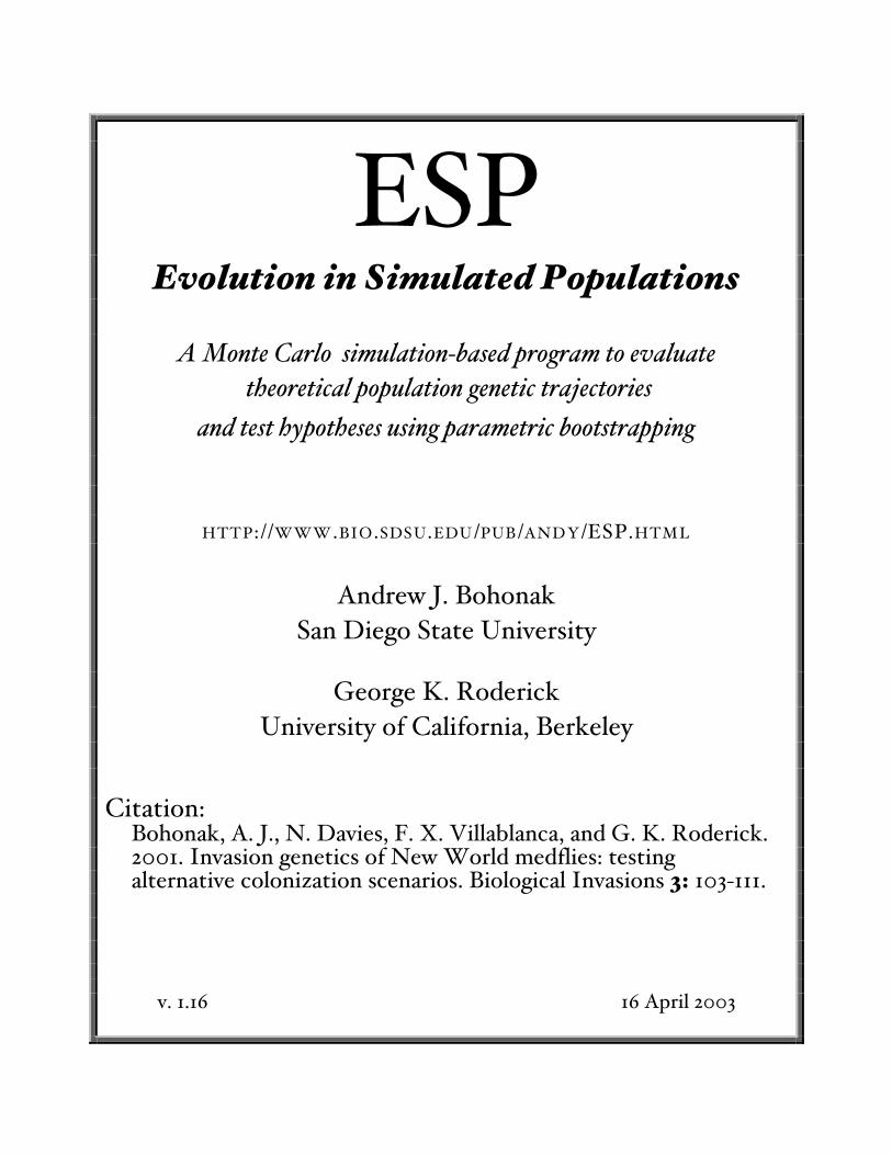
population genetics requires two primary decisions. First, complex, multivariate data setsneed to be reduced to simpler summary statistics or analytic frameworks. Second, nullhypotheses must be evaluated using theoretical expectations that account for appropriatesources of variation. Traditionally, stochastic and/or sampling variation (sensu Slatkin andArter 1991) have been considered when constructing population genetic null models.However, initial state variation can be as important as stochastic and sampling variationwhen 1) the hypothesis is designed to infer process, rather than simply describe pattern and2) the populations are not at an equilibrium between drift, mutation and gene flow (seeFigure 1). For example, suppose that very low values of heterozygosity are found in aparticular population. In order to generate a null distribution for a founding event by ncolonists, one must consider the among-population variation that results from randomsamples of 2n genes from the ancestral pool (e.g., Hairston et al. 1999, Bohonak et al. inpress). Initial state variation also consists of differences among population sets that havebeen randomly founded by the same process.

Over time, the influence of these founder effects decays, initial state variationbecomes less important, and eventually the level of population differentiation reaches abalance between migration, mutation and random genetic drift. Natural selection will alsobe important for traits not evolving under neutrality. Because of these complexities,interpretations of population differentiation are context-dependent and usually open todebate. It is often difficult to determine whether populations are old enough to havereached a drift-gene flow-mutation equilibrium, and if they are not at equilibrium, multiplecolonization scenarios may be consistent with the observed patterns. For very youngpopulations (e.g., invading species) unambiguous interpretations can particularly difficult.

{

Populationparameter

(e.g., F , H )ST e

T i m e

} stochastic variation,parametric variation

Initial state variation

estimation

frequency distribution

} statistical variation

Figure 1. Four sources of variation for population genetic statistics. Each line represents one group of populations;the three solid lines all begin with the same initial state.

ESP Manual

3

General coverage of these topics can be found in Hartl and Clark (1997), and in numerousreviews (e.g., Slatkin 1985, Avise 1994, Roderick 1996, Bohonak 1999).

With these motivations, we have written ESP in order to provide a framework forevaluating population differentiation over time while accommodating stochastic variation,statistical variation and variation in initial state. ESP provides a general, Monte Carlo-based algorithm to generate null distributions via parametric bootstrapping. The programhas, in our view, at least four uses:

1. To evaluate the likelihood of particular values for population parameters such as rate ofgene flow and effective population size.

2. To evaluate the likelihood of particular colonization scenarios.

3. To provide guidance when designing a sampling regime and choosing molecular markers.

4. To provide a teaching tool that illustrates how gene genealogies evolve over time in thecontext of drift, gene flow and mutation.

Style conventionsThroughout this manual, references to other sections of the manual appear in a

larger font (e.g., Parameters and Settings), variables and statistics appear in italics (e.g.,FST), program options and screen output appear in bold Monaco (e.g., # populations),and examples of ESP outfiles are represented in small Geneva (e.g., Alleles saved by ESP v0.7).

Getting startedHardware

ESP for Power Macintosh requires from 10 MB to more than 50 MB of RAM,depending on simulation size (see Performance below). For large simulations, a G3 or G4processor is suggested. Extensive testing as been conducted using Systems 8.5 through 9.1on G3 (including iMacs) and G4 processors, although the application may also run well onother operating system versions.

Software installationInstallation of ESP only requires downloading and expanding the SEA (self

expanding archive) available on the ESP web site. If the default RAM requirements are

ESP Manual

4

inappropriate for a particular set of simulations, they can be changed manually within theMacintosh finder (through the Get Info->Memory menu). Unfortunately, large simulationswill dominate processing power, so that users will find it easiest not to run ESP in thebackground.

OperationThere are essentially four phases to population genetic analyses with ESP.

1. First, customize population parameters and output analyses from the opening screen.2. Second, start ESP by entering <y>.3. Summary statistics from one or more Monte Carlo simulations appear on the screen as

the populations interact and evolve over time. More extensive output is saved as a tab-formatted text file in the ESP folder.

4. ESP outfiles can be easily viewed and manipulated in a spreadsheet such as MicrosoftExcel. The outfiles are column-formatted in a manner that makes graphing the resultsrelatively straightforward. The screen output buffer may also be sent directly to aprinter.

5. When quitting ESP. the user is prompted to "save before quitting". This will save thescreen buffer, which is usually not necessary, because outfiles are saved after eachMonte Carlo simulation by default.

Additional options are described below.

Program overviewESP utilizes Monte Carlo simulations to simulate the evolutionary process, and

calculates summary statistics which incorporate initial state variation, stochastic variationand statistical variation (described in Bohonak and Roderick, submitted). ESP keeps track ofeach allele's* genealogical relationship to other alleles and an array of its frequency in eachpopulation. Migration, mutation and reproduction are simulated as simple Poissonprocesses, assuming that mating is random and that each individual contributes a largenumber of gametes to the gamete pool (the standard Wright-Fisher model). Mutation istreated as an infinite-allele model, and as a result, sequence convergence and saturation arenot considered (i.e., the relationships among alleles are always known). Stepwise mutations(for microsatellites) are not currently incorporated.

Gene flow follows a simple island model. Under some conditions (low migrationrates, very young and/or very large populations), founder effects will dominate patterns of

* For clarity, allele is used throughout this manual to identify unique genes in the gene pool. In contrast,haplotype will be used generically to refer to all members of the gene pool, whether or not they areunique. Thus, a haplotype might consist of a 1000 bp length of DNA or a "1 bp" allozyme locus. Thenumber of haplotypes in a diploid gene pool is twice the effective population size.

ESP Manual

5

differentiation, and few qualitative differences might be expected between island andspatially explicit models of migration. Future versions of the program will incorporateadditional migration patterns.

A wide variety of initial conditions are permitted. Populations can be foundedthrough an algorithm that approximates the desired initial value of FST, or through a flexibleGeneral Colonization Algorithm (GCA). The GCA permits populations to be randomlyfounded from randomly generated or empirical data sets in numerous ways.

Confidence intervals can be generated across multiple replicates for one or morepoints in time, and for one or more summary statistics. These confidence intervals can becompared to empirical data to test hypotheses via 'parametric bootstrapping'.

The program’s accuracy and robustness have been tested by extensively varyingparameters such as sequence length, mutation rate, number and size of populations,migration rate and initial population structure. Rates of divergence and equilibrium valuesfor population differentiation generally agree with theoretical expectations (e.g.,Cockerham and Weir 1987, Slatkin 1994, Hartl and Clark 1997). Algorithms for calculatingθ and ΦS T have been verified by comparisons with output from Schneider et al.’s (1998)Arlequin and Miller's (1998) TFPGA.

Critiques, suggestions, commentary and bug reports are welcomed. Sende m a i l t o <bohonak@sciences.sdsu.edu> and include the version number anderror number (if applicable). Updates will be made available periodically at<http://www.bio.sdsu.edu/pub/andy/ESP.html>.

Parameters and settingsUser-defined

Upon launching the program, the values of approximately 20 parameters and settingsare displayed. ESP utilizes a preferences file that is placed in the program folder, so thatthese settings are retained after the program is quit. If the preferences file is absent, theprogram will revert to defaults and create a new preferences file.

g # generations Zero to 4 million.

? print every 50 gens How often summary statistics will be calculated and printed

n 2 x population size The population size in haplotypes. (For a diploid organism, this willbe equivalent to 2Ne). Limitations are outlined in Parameter limitsbelow.

ESP Manual

6

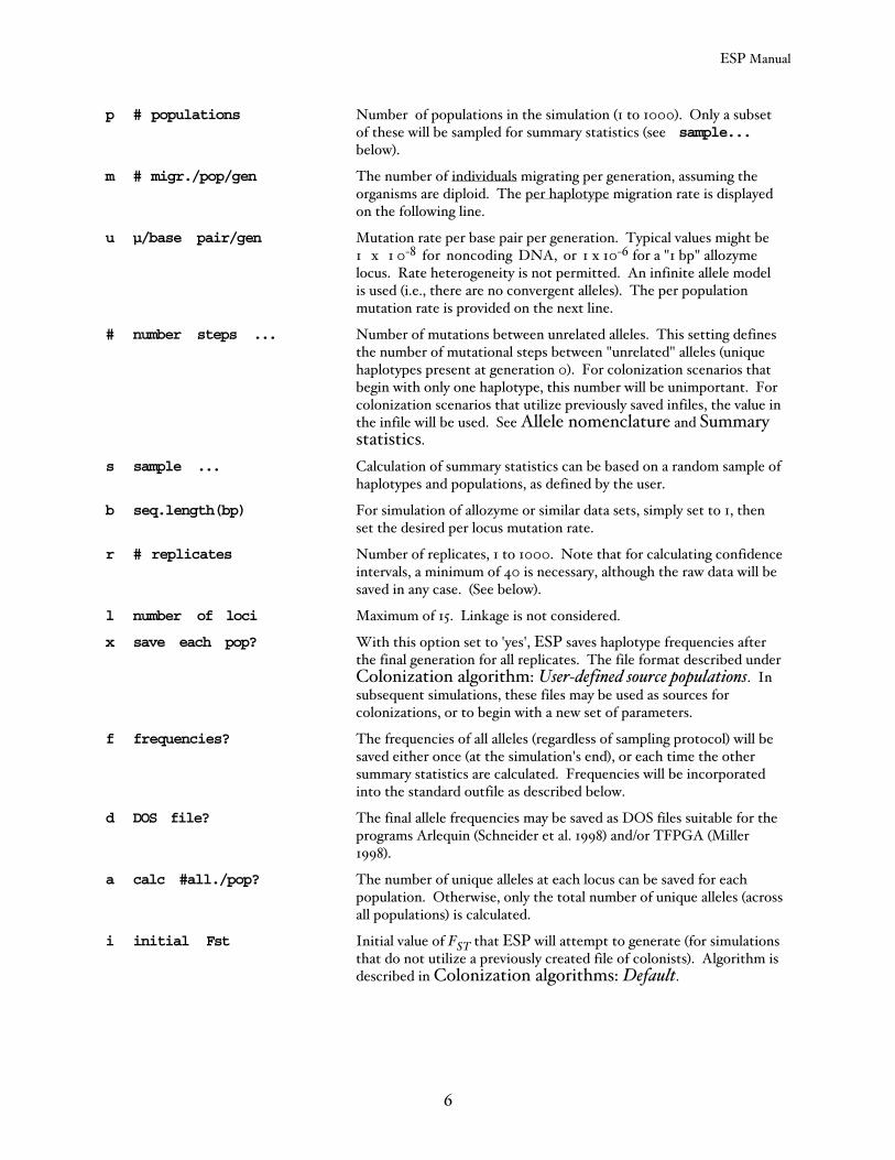
p # populations Number of populations in the simulation (1 to 1000). Only a subsetof these will be sampled for summary statistics (see sample...below).

m # migr./pop/gen The number of individuals migrating per generation, assuming theorganisms are diploid. The per haplotype migration rate is displayedon the following line.

u µ/base pair/gen Mutation rate per base pair per generation. Typical values might be1 x 1 0-8 for noncoding DNA, or 1 x 10-6 for a "1 bp" allozymelocus. Rate heterogeneity is not permitted. An infinite allele modelis used (i.e., there are no convergent alleles). The per populationmutation rate is provided on the next line.

# number steps ... Number of mutations between unrelated alleles. This setting definesthe number of mutational steps between "unrelated" alleles (uniquehaplotypes present at generation 0). For colonization scenarios thatbegin with only one haplotype, this number will be unimportant. Forcolonization scenarios that utilize previously saved infiles, the value inthe infile will be used. See Allele nomenclature and Summarystatistics.

s sample ... Calculation of summary statistics can be based on a random sample ofhaplotypes and populations, as defined by the user.

b seq.length(bp) For simulation of allozyme or similar data sets, simply set to 1, thenset the desired per locus mutation rate.

r # replicates Number of replicates, 1 to 1000. Note that for calculating confidenceintervals, a minimum of 40 is necessary, although the raw data will besaved in any case. (See below).

l number of loci Maximum of 15. Linkage is not considered.

x save each pop? With this option set to 'yes', ESP saves haplotype frequencies afterthe final generation for all replicates. The file format described underColonization algorithm: User-defined source populations. Insubsequent simulations, these files may be used as sources forcolonizations, or to begin with a new set of parameters.

f frequencies? The frequencies of all alleles (regardless of sampling protocol) will besaved either once (at the simulation's end), or each time the othersummary statistics are calculated. Frequencies will be incorporatedinto the standard outfile as described below.

d DOS file? The final allele frequencies may be saved as DOS files suitable for theprograms Arlequin (Schneider et al. 1998) and/or TFPGA (Miller1998).

a calc #all./pop? The number of unique alleles at each locus can be saved for eachpopulation. Otherwise, only the total number of unique alleles (acrossall populations) is calculated.

i initial Fst Initial value of FST that ESP will attempt to generate (for simulationsthat do not utilize a previously created file of colonists). Algorithm isdescribed in Colonization algorithms: Default.

ESP Manual

7

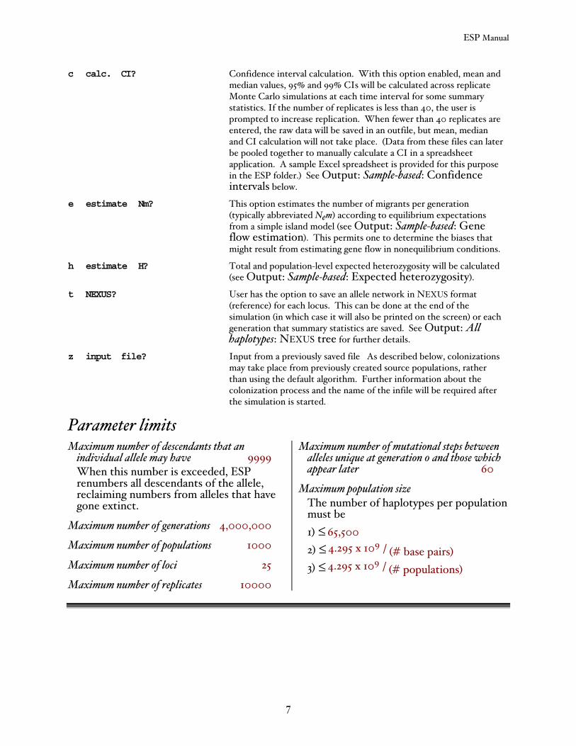
c calc. CI? Confidence interval calculation. With this option enabled, mean andmedian values, 95% and 99% CIs will be calculated across replicateMonte Carlo simulations at each time interval for some summarystatistics. If the number of replicates is less than 40, the user isprompted to increase replication. When fewer than 40 replicates areentered, the raw data will be saved in an outfile, but mean, medianand CI calculation will not take place. (Data from these files can laterbe pooled together to manually calculate a CI in a spreadsheetapplication. A sample Excel spreadsheet is provided for this purposein the ESP folder.) See Output: Sample-based: Confidenceintervals below.

e estimate Nm? This option estimates the number of migrants per generation(typically abbreviated Nem) according to equilibrium expectationsfrom a simple island model (see Output: Sample-based: Geneflow estimation). This permits one to determine the biases thatmight result from estimating gene flow in nonequilibrium conditions.

h estimate H? Total and population-level expected heterozygosity will be calculated(see Output: Sample-based: Expected heterozygosity).

t NEXUS? User has the option to save an allele network in NEXUS format(reference) for each locus. This can be done at the end of thesimulation (in which case it will also be printed on the screen) or eachgeneration that summary statistics are saved. See Output: Allhaplotypes: NEXUS tree for further details.

z input file? Input from a previously saved file As described below, colonizationsmay take place from previously created source populations, ratherthan using the default algorithm. Further information about thecolonization process and the name of the infile will be required afterthe simulation is started.

Parameter limitsMaximum number of descendants that an

individual allele may have 9999When this number is exceeded, ESPrenumbers all descendants of the allele,reclaiming numbers from alleles that havegone extinct.

Maximum number of generations 4,000,000Maximum number of populations 1000Maximum number of loci 25Maximum number of replicates 10000

Maximum number of mutational steps betweenalleles unique at generation 0 and those whichappear later 60

Maximum population sizeThe number of haplotypes per populationmust be1) ≤ 65,5002) ≤ 4.295 x 109 / (# base pairs)3) ≤ 4.295 x 109 / (# populations)

ESP Manual

8

Colonization algorithmsThe manner in which populations are founded in nature will dramatically affect their

initial levels of divergence; similarly, the choice of initial conditions in an ESP simulationcan dramatically affect its outcome. One of ESP's primary uses is to quantify the persistenteffects of bottlenecks and founder effects on population differentiation. As a result,populations can be colonized in a wide variety of ways.

DefaultWhen input file? is turned off, initial values of FST are approximated by the

following algorithms. Define P to be the number of populations in the simulation, 2Ne tobe the effective population size in haplotypes and F0 to be the target value for FST atgeneration 0:

F0 = 0: When initial Fst is set to zero, the user will be prompted for an initialnumber of alleles at each locus, and then for their initial frequencies. Allpopulations begin with this same configuration.

F0 = 1: Each population begins with a single, unique allele.

0 < F0 < 1: At generation 0, P haplotypes are temporarily created for each locus; each is afixed number of mutational steps apart (see Parameters and Settings: User-defined: number steps…). One of these alleles is chosen randomly, and 2Ne*F0haplotypes in population 1 are assigned this allele's identity. This process isrepeated until all 2Ne haplotypes are assigned to population 1. Allele identitiesare assigned to each remaining population in the same manner. (Algorithmderived from discussion in Wade and McCauley 1988). Unused haplotypes arethen eliminated before the simulation continues.

This algorithm provides an acceptable approximation when 2Ne and P are large. Formore control over the colonization process, create user-defined source populationsmanually, or with prior simulations.

"ESP freqs" infilesWhen input file? is turned on, ESP samples external files in order to found new

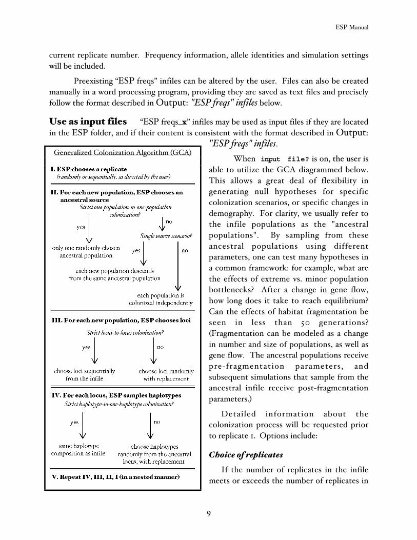
populations at generation 0. These infiles may be created from an ESP simulation, ormanually. ESP's Generalized Colonization Algorithm (GCA) can then be used to simulatecolonization events of almost any type (see diagram below).

Creating infiles With the save each pop? setting activated, a file will be createdfor all of the replicates in a particular run. Files will be named “ESP freqs_x”, where x is the

ESP Manual

9

current replicate number. Frequency information, allele identities and simulation settingswill be included.

Preexisting “ESP freqs” infiles can be altered by the user. Files can also be createdmanually in a word processing program, providing they are saved as text files and preciselyfollow the format described in Output: "ESP freqs" infiles below.

Use as input files “ESP freqs_x” infiles may be used as input files if they are locatedin the ESP folder, and if their content is consistent with the format described in Output:

"ESP freqs" infiles.When input file? is on, the user is

able to utilize the GCA diagrammed below.This allows a great deal of flexibility ingenerating null hypotheses for specificcolonization scenarios, or specific changes indemography. For clarity, we usually refer tothe infile populations as the "ancestralpopulations". By sampling from theseancestral populations using differentparameters, one can test many hypotheses ina common framework: for example, what arethe effects of extreme vs. minor populationbottlenecks? After a change in gene flow,how long does it take to reach equilibrium?Can the effects of habitat fragmentation beseen in less than 50 generations?(Fragmentation can be modeled as a changein number and size of populations, as well asgene flow. The ancestral populations receivepre-fragmentation parameters, andsubsequent simulations that sample from theancestral infile receive post-fragmentationparameters.)

Detailed information about thecolonization process will be requested priorto replicate 1. Options include:

Choice of replicatesIf the number of replicates in the infile

meets or exceeds the number of replicates in

Generalized Colonization Algorithm (GCA)

ESP Manual

10

the current run, the ancestral replicates can be used sequentially, or sampled randomlywith replacement.

The random replicate option is automatically used when there is only one replicatein the current run, or the number of replicates in the infile is less than the number ofreplicates in the current run.

Choice of lociIf the number of loci in the infile equals the number of loci in the current run, the

loci can be used sequentially in a strict ancestral locus-t0-new locus fashion. Otherwise,the new loci are sampled randomly with replacement from the infile.

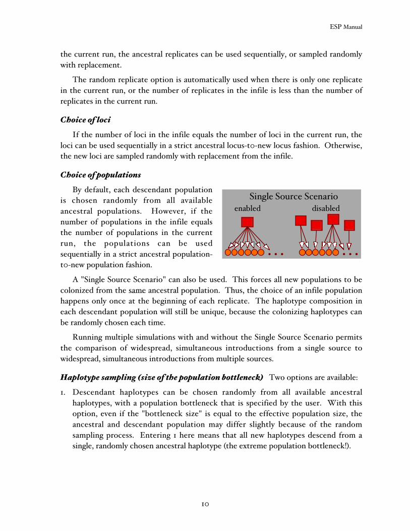
Choice of populationsBy default, each descendant population

is chosen randomly from all availableancestral populations. However, if thenumber of populations in the infile equalsthe number of populations in the currentrun, the populations can be usedsequentially in a strict ancestral population-t0-new population fashion.

A "Single Source Scenario" can also be used. This forces all new populations to becolonized from the same ancestral population. Thus, the choice of an infile populationhappens only once at the beginning of each replicate. The haplotype composition ineach descendant population will still be unique, because the colonizing haplotypes canbe randomly chosen each time.

Running multiple simulations with and without the Single Source Scenario permitsthe comparison of widespread, simultaneous introductions from a single source towidespread, simultaneous introductions from multiple sources.

Haplotype sampling (size of the population bottleneck) Two options are available:

1. Descendant haplotypes can be chosen randomly from all available ancestralhaplotypes, with a population bottleneck that is specified by the user. With thisoption, even if the "bottleneck size" is equal to the effective population size, theancestral and descendant population may differ slightly because of the randomsampling process. Entering 1 here means that all new haplotypes descend from asingle, randomly chosen ancestral haplotype (the extreme population bottleneck!).

Single Source Scenarioenabled

. . .

disabled

. . .

ESP Manual

11

2 . Colonizations can occur in a strict one-ancestral-haplotype to one-descendant-haplotype fashion. For this option, the population size of the infile must equal thepopulation size of the current simulation.

Allele nomenclatureBy default, ESP names alleles in a genealogically informative manner. Unique alleles

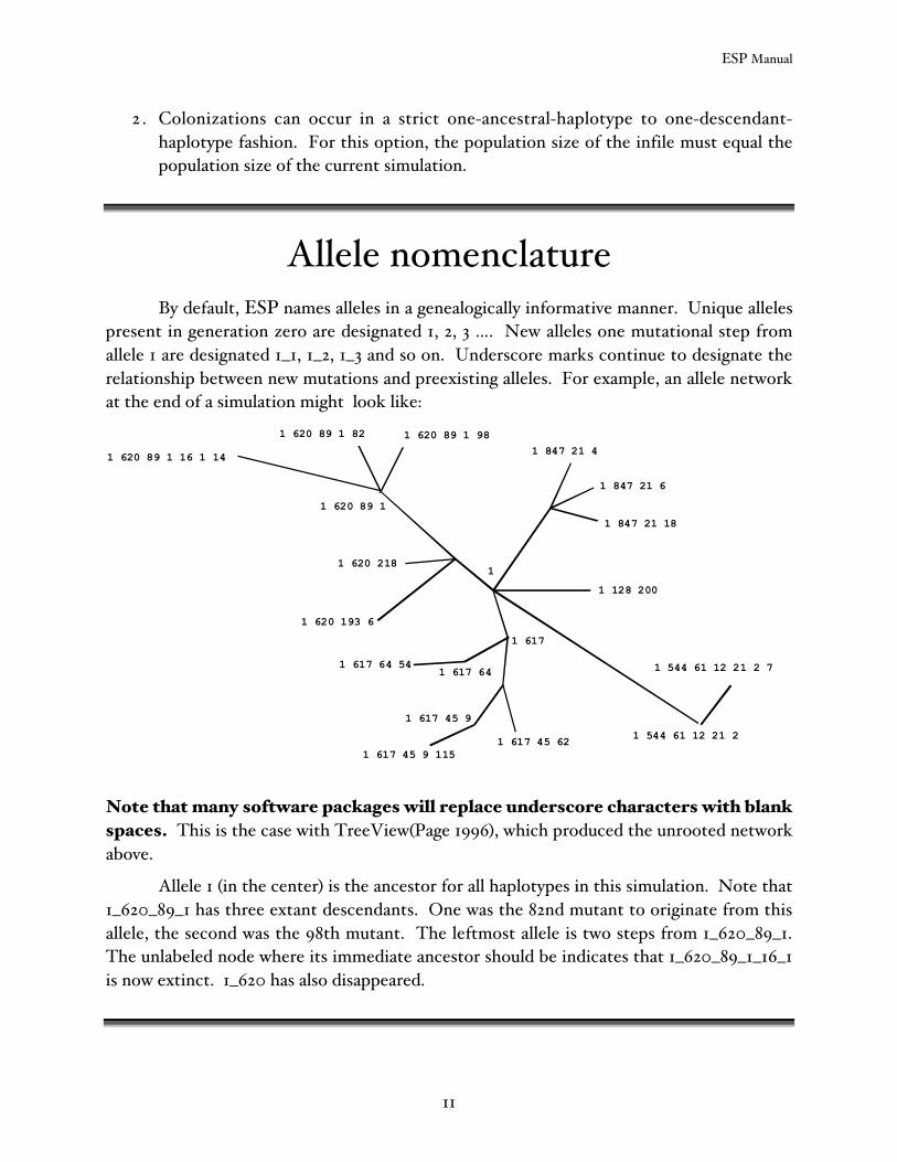
present in generation zero are designated 1, 2, 3 …. New alleles one mutational step fromallele 1 are designated 1_1, 1_2, 1_3 and so on. Underscore marks continue to designate therelationship between new mutations and preexisting alleles. For example, an allele networkat the end of a simulation might look like:

1 128 200

1 544 61 12 21 2

1 544 61 12 21 2 7

1 617

1 617 45 62

1 617 45 9

1 617 45 9 115

1 617 641 617 64 54

1 620 193 6

1 620 218

1 620 89 1

1 620 89 1 16 1 14

1 620 89 1 82 1 620 89 1 981 847 21 4

1 847 21 6

1 847 21 18

1

Note that many software packages will replace underscore characters with blankspaces. This is the case with TreeView(Page 1996), which produced the unrooted networkabove.

Allele 1 (in the center) is the ancestor for all haplotypes in this simulation. Note that1_620_89_1 has three extant descendants. One was the 82nd mutant to originate from thisallele, the second was the 98th mutant. The leftmost allele is two steps from 1_620_89_1.The unlabeled node where its immediate ancestor should be indicates that 1_620_89_1_16_1is now extinct. 1_620 has also disappeared.

ESP Manual

12

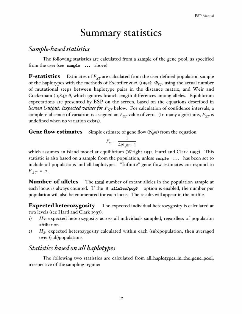
Summary statisticsSample-based statistics

The following statistics are calculated from a sample of the gene pool, as specifiedfrom the user (see sample ... above).

F-statistics Estimates of FST are calculated from the user-defined population sampleof the haplotypes with the methods of Excoffier et al. (1992): ΦST, using the actual numberof mutational steps between haplotype pairs in the distance matrix, and Weir andCockerham (1984): θ, which ignores branch length differences among alleles. Equilibriumexpectations are presented by ESP on the screen, based on the equations described inScreen Output: Expected values for FST below. For calculation of confidence intervals, acomplete absence of variation is assigned an FST value of zero. (In many algorithms, FST isundefined when no variation exists).

Gene flow estimates Simple estimate of gene flow (Nem) from the equation

F

N mSTe

=+

14 1

which assumes an island model at equilibrium (Wright 1931, Hartl and Clark 1997). Thisstatistic is also based on a sample from the population, unless sample ... has been set toinclude all populations and all haplotypes. "Infinite" gene flow estimates correspond toF S T = 0 .

Number of alleles The total number of extant alleles in the population sample ateach locus is always counted. If the # alleles/pop? option is enabled, the number perpopulation will also be enumerated for each locus. The results will appear in the outfile.

Expected heterozygosity The expected individual heterozygosity is calculated attwo levels (see Hartl and Clark 1997):1) HT: expected heterozygosity across all individuals sampled, regardless of population

affiliation.2) HS: expected heterozygosity calculated within each (sub)population, then averaged

over (sub)populations.

Statistics based on all haplotypesThe following two statistics are calculated from all haplotypes in the gene pool,

irrespective of the sampling regime:

ESP Manual

13

Allele frequencies When the frequencies? option is toggled, the frequencies ofeach allele will be calculated either each time summary statistics are generated, or only atthe end of the simulation. These frequencies are always based on the entire gene pool, andappear in the outfile.

NEXUS tree With the NEXUS tree? option enabled, ESP will generate NEXUS code(Maddison et al. 1997) so that a picture of the allele network may be generated in programssuch as TreeView (Page 1996). Note that this will consist of all haplotypes in all populationsat each locus. Also note that population-specific trees will not be generated and thatTreeView has a maximum of 500 alleles. The NEXUS code will appear on the screen, and ina text-only outfile.

If desired, ESP will use sequential labels in this code (1,2,3 …) rather thangenealogically informative labels. This may be desired if allele names become excessivelylong. Correct NEXUS code will result in either case.

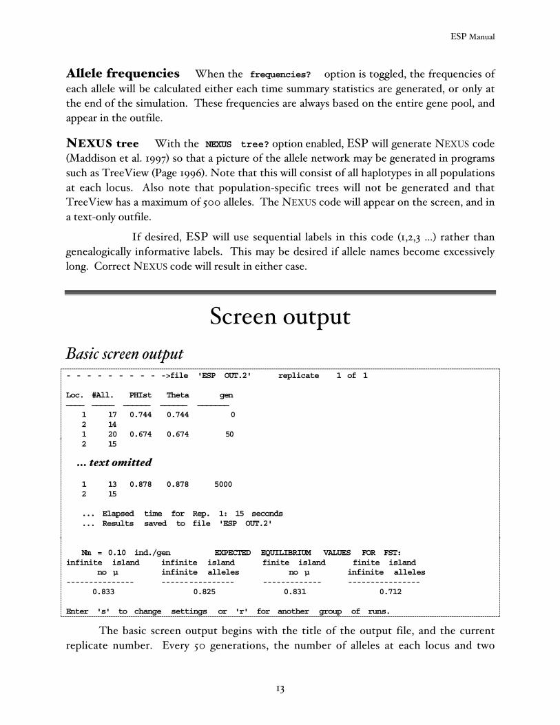
Screen outputBasic screen output- - - - - - - - - ->file 'ESP OUT.2' replicate 1 of 1

Loc. #All. PHIst Theta gen———— ————— —————— —————— ——————— 1 17 0.744 0.744 0 2 14 1 20 0.674 0.674 50 2 15

… text omitted 1 13 0.878 0.878 5000 2 15

... Elapsed time for Rep. 1: 15 seconds ... Results saved to file 'ESP OUT.2'

Nm = 0.10 ind./gen EXPECTED EQUILIBRIUM VALUES FOR FST:infinite island infinite island finite island finite island no µ infinite alleles no µ infinite alleles--------------- ---------------- ------------- ---------------- 0.833 0.825 0.831 0.712

Enter 's' to change settings or 'r' for another group of runs.

The basic screen output begins with the title of the output file, and the currentreplicate number. Every 50 generations, the number of alleles at each locus and two

ESP Manual

14

estimates of FST are calculated from the user-defined sample size. (Note that colonizationoccurs at generation 0, and that the statistics calculated at generation 0 come before anygene flow, drift or mutation). After the final generation, the elapsed time is provided, andESP verifies that the outfile has been written. The amount of gene flow (# migratinghaplotypes per generation) is printed, followed by four equilibrium expectations for FST (seeExpected values for FST). ESP prompts the user to continue.

The screen output buffer may be printed or saved as a text file. However, the outfilesaved by ESP provides more information. Outfiles can also be more easily input into aspreadsheet program than copied screen text, because they are tab-delimited, rather thanfixed width.

Optional settingsScreen output will also contain estimates of Nem if estimate Nm? is enabled, and

expected heterozygosity (total and (sub)population) if estimate H? is enabled. (Allelefrequencies and the number of alleles per population will appear in the outfile if theappropriate settings are enabled, but are not printed on the screen), If NEXUS tree? isturned on, NEXUS code will appear at the conclusion of the simulation for each locus (seeNEXUS above). If additional DOS outfiles are created, a notification will appear on thescreen.

If the GCA is used to begin the simulation and random population sampling ischosen, screen output will reflect which populations are being sampled. This list will notappear in the outfile, although a summary of the available infiles will.

ESP Manual

15

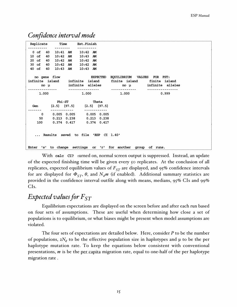
Confidence interval mode Replicate Time Est.Finish---------- -------- ---------- 0 of 40 10:41 AM 10:42 AM 10 of 40 10:42 AM 10:43 AM 20 of 40 10:42 AM 10:42 AM 30 of 40 10:42 AM 10:42 AM 40 of 40 10:43 AM 10:43 AM

no gene flow EXPECTED EQUILIBRIUM VALUES FOR FST:infinite island infinite island finite island finite island no µ infinite alleles no µ infinite alleles--------------- ---------------- ------------- ---------------- 1.000 1.000 1.000 0.999

Phi-ST Theta Gen [2.5] [97.5] [2.5] [97.5]------- ------------ ------------ 0 0.005 0.005 0.005 0.005 50 0.213 0.238 0.213 0.238 100 0.374 0.417 0.374 0.417

... Results saved to file 'ESP CI 1.40'

Enter 's' to change settings or 'r' for another group of runs.

With calc CI? turned on, normal screen output is suppressed. Instead, an updateof the expected finishing time will be given every 50 replicates. At the conclusion of allreplicates, expected equilibrium values of FST are displayed, and 95% confidence intervalsfor are displayed for ΦST, θ , and N em (if enabled). Additional summary statistics areprovided in the confidence interval outfile along with means, medians, 95% CIs and 99%CIs.

Expected values for FSTEquilibrium expectations are displayed on the screen before and after each run based

on four sets of assumptions. These are useful when determining how close a set ofpopulations is to equilibrium, or what biases might be present when model assumptions areviolated.

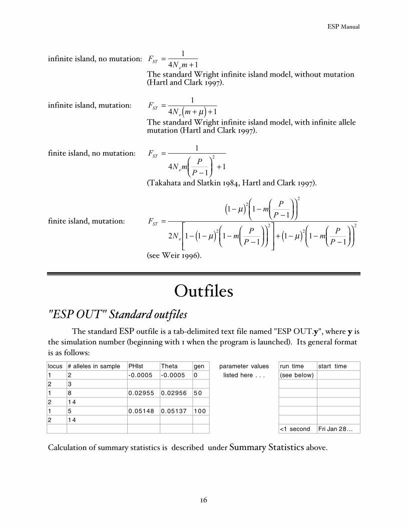
The four sets of expectations are detailed below. Here, consider P to be the numberof populations, 2Ne to be the effective population size in haplotypes and µ to be the perhaplotype mutation rate. To keep the equations below consistent with conventionalpresentations, m is be the per capita migration rate, equal to one-half of the per haplotypemigration rate .

ESP Manual

16

infinite island, no mutation: F

N mSTe

=+

14 1

The standard Wright infinite island model, without mutation(Hartl and Clark 1997).

infinite island, mutation: F

N mSTe

=+( ) +1

4 1µThe standard Wright infinite island model, with infinite allelemutation (Hartl and Clark 1997).

finite island, no mutation:

F

N mP

P

ST

e

=

−

+

1

41

12

(Takahata and Slatkin 1984, Hartl and Clark 1997).

finite island, mutation:

F

mP

P

N mP

Pm

PP

ST

e

=−( ) −

−

− −( ) −−

+ −( ) −−

1 11

2 1 1 11

1 11

22

22

22

µ

µ µ

(see Weir 1996).

Outfiles"ESP OUT" Standard outfiles

The standard ESP outfile is a tab-delimited text file named "ESP OUT.y", where y isthe simulation number (beginning with 1 when the program is launched). Its general formatis as follows:locus # alleles in sample PHIst Theta gen parameter values run time start time

1 2 -0.0005 -0.0005 0 listed here . . . (see below)

2 3

1 8 0.02955 0.02956 5 0

2 1 4

1 5 0.05148 0.05137 100

2 1 4

<1 second Fri Jan 28…

Calculation of summary statistics is described under Summary Statistics above.

ESP Manual

17

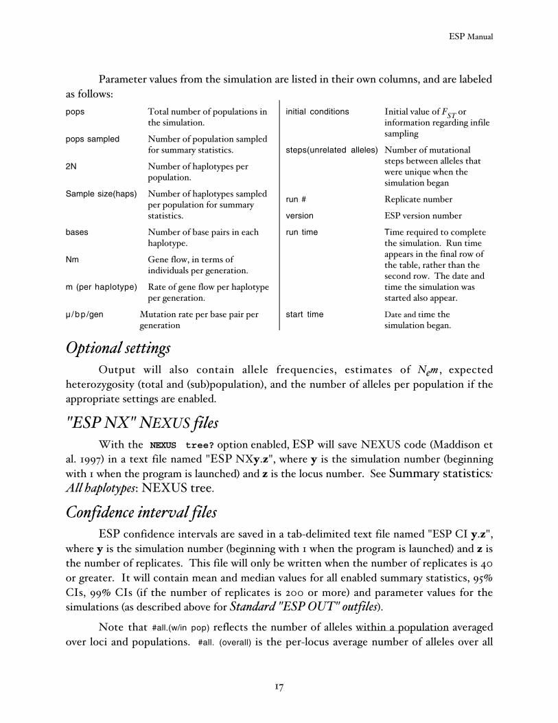
Parameter values from the simulation are listed in their own columns, and are labeledas follows:pops Total number of populations in

the simulation.

pops sampled Number of population sampledfor summary statistics.

2N Number of haplotypes perpopulation.

Sample size(haps) Number of haplotypes sampledper population for summarystatistics.

bases Number of base pairs in eachhaplotype.

Nm Gene flow, in terms ofindividuals per generation.

m (per haplotype) Rate of gene flow per haplotypeper generation.

µ /bp /gen Mutation rate per base pair pergeneration

initial conditions Initial value of FST orinformation regarding infilesampling

steps(unrelated alleles) Number of mutationalsteps between alleles thatwere unique when thesimulation began

run # Replicate number

version ESP version number

run time Time required to completethe simulation. Run timeappears in the final row ofthe table, rather than thesecond row. The date andtime the simulation wasstarted also appear.

start time Date and time thesimulation began.

Optional settingsOutput will also contain allele frequencies, estimates of Nem , expected

heterozygosity (total and (sub)population), and the number of alleles per population if theappropriate settings are enabled.

"ESP NX" NEXUS filesWith the NEXUS tree? option enabled, ESP will save NEXUS code (Maddison et

al. 1997) in a text file named "ESP NXy.z", where y is the simulation number (beginningwith 1 when the program is launched) and z is the locus number. See Summary statistics:All haplotypes: NEXUS tree.

Confidence interval filesESP confidence intervals are saved in a tab-delimited text file named "ESP CI y.z",

where y is the simulation number (beginning with 1 when the program is launched) and z isthe number of replicates. This file will only be written when the number of replicates is 40or greater. It will contain mean and median values for all enabled summary statistics, 95%CIs, 99% CIs (if the number of replicates is 200 or more) and parameter values for thesimulations (as described above for Standard "ESP OUT" outfiles).

Note that #all.(w/in pop) reflects the number of alleles within a population averagedover loci and populations. #all. (overall) is the per-locus average number of alleles over all

ESP Manual

18

populations. For example, three populations with fixed differences might have one alleleeach (within population) but there would be three alleles (overall) at that locus.

"ESP CI data" filesIn the event that a set of confidence interval simulations is prematurely terminated,

some of the replicates can be recovered. Every 50 replicates, ESP saves all of the datacollected to that point in time in a file labeled "ESP CI data.z", where z is the number ofthe current replicate. (Each CI data file is a superset of the file preceding it).

To calculate confidence intervals other than those provided, or to pool data fromdifferent CI data files, the raw data can be imported into a spreadsheet application andsorted. A sample spreadsheet for Microsoft Excel is provided in the ESP folder.

When the gene flow estimation option is on, infinite gene flow (corresponding toFST = 0) is coded in the ESP CI data files as -99.

"arleq" and "TFPGA" DOS outfilesDOS outfiles for the programs Arlequin (Schneider et al. 1998) and TFPGA (Miller

1998) are formatted according to the documentation that accompanies those programs.The replicate number appears in the file name, and some information on simulationparameters appears in the remarks section of each file.

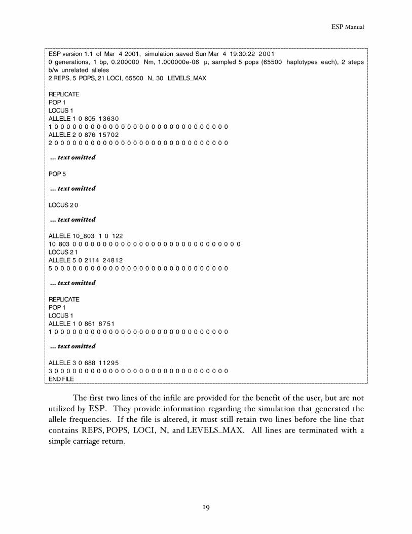
"ESP freqs" infilesESP infiles are text-only files named “ESP freqs_x”, where x represents the replicate.

In order to sample from these infiles for colonization/fragmentation scenarios, they mustremain in the same folder as the application. The file format is follows on the next page:

ESP Manual

19

ESP version 1.1 of Mar 4 2001, simulation saved Sun Mar 4 19:30:22 20010 generations, 1 bp, 0.200000 Nm, 1.000000e-06 µ, sampled 5 pops (65500 haplotypes each), 2 stepsb/w unrelated alleles2 REPS, 5 POPS, 21 LOCI, 65500 N, 30 LEVELS_MAX

REPLICATEPOP 1LOCUS 1ALLELE 1 0 805 136301 0 0 0 0 0 0 0 0 0 0 0 0 0 0 0 0 0 0 0 0 0 0 0 0 0 0 0 0 0ALLELE 2 0 876 157022 0 0 0 0 0 0 0 0 0 0 0 0 0 0 0 0 0 0 0 0 0 0 0 0 0 0 0 0 0

… text omitted

POP 5

… text omitted

LOCUS 2 0

… text omitted

ALLELE 10_803 1 0 12210 803 0 0 0 0 0 0 0 0 0 0 0 0 0 0 0 0 0 0 0 0 0 0 0 0 0 0 0 0LOCUS 2 1ALLELE 5 0 2114 248125 0 0 0 0 0 0 0 0 0 0 0 0 0 0 0 0 0 0 0 0 0 0 0 0 0 0 0 0 0

… text omitted

REPLICATEPOP 1LOCUS 1ALLELE 1 0 861 87511 0 0 0 0 0 0 0 0 0 0 0 0 0 0 0 0 0 0 0 0 0 0 0 0 0 0 0 0 0

… text omitted

ALLELE 3 0 688 112953 0 0 0 0 0 0 0 0 0 0 0 0 0 0 0 0 0 0 0 0 0 0 0 0 0 0 0 0 0END FILE

The first two lines of the infile are provided for the benefit of the user, but are notutilized by ESP. They provide information regarding the simulation that generated theallele frequencies. If the file is altered, it must still retain two lines before the line thatcontains REPS, POPS, LOCI, N, and LEVELS_MAX. All lines are terminated with asimple carriage return.

ESP Manual

20

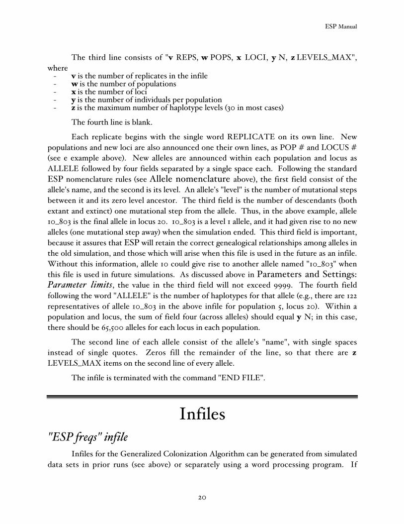
The third line consists of "v REPS, w POPS, x LOCI, y N, z LEVELS_MAX",where

- v is the number of replicates in the infile- w is the number of populations- x is the number of loci- y is the number of individuals per population- z is the maximum number of haplotype levels (30 in most cases)

The fourth line is blank.

Each replicate begins with the single word REPLICATE on its own line. Newpopulations and new loci are also announced one their own lines, as POP # and LOCUS #(see e example above). New alleles are announced within each population and locus asALLELE followed by four fields separated by a single space each. Following the standardESP nomenclature rules (see Allele nomenclature above), the first field consist of theallele's name, and the second is its level. An allele's "level" is the number of mutational stepsbetween it and its zero level ancestor. The third field is the number of descendants (bothextant and extinct) one mutational step from the allele. Thus, in the above example, allele10_803 is the final allele in locus 20. 10_803 is a level 1 allele, and it had given rise to no newalleles (one mutational step away) when the simulation ended. This third field is important,because it assures that ESP will retain the correct genealogical relationships among alleles inthe old simulation, and those which will arise when this file is used in the future as an infile.Without this information, allele 10 could give rise to another allele named "10_803" whenthis file is used in future simulations. As discussed above in Parameters and Settings:Parameter limits, the value in the third field will not exceed 9999. The fourth fieldfollowing the word "ALLELE" is the number of haplotypes for that allele (e.g., there are 122representatives of allele 10_803 in the above infile for population 5, locus 20). Within apopulation and locus, the sum of field four (across alleles) should equal y N; in this case,there should be 65,500 alleles for each locus in each population.

The second line of each allele consist of the allele's "name", with single spacesinstead of single quotes. Zeros fill the remainder of the line, so that there are zLEVELS_MAX items on the second line of every allele.

The infile is terminated with the command "END FILE".

Infiles"ESP freqs" infile

Infiles for the Generalized Colonization Algorithm can be generated from simulateddata sets in prior runs (see above) or separately using a word processing program. If

ESP Manual

21

generated by the user, the infiles must be saved as “text only”, named “ESP freqs_x”, wherex is a number, and be in the same folder as the application. The file format must follow thatdescribed in the preceeding section, except that alleles can be given any names. (However,ESP will ignore the user-specified name, and designate alleles according to thenomenclature described under Allele Nomenclature.)

PerformanceESP simulates the evolution of gene genealogies relatively quickly, but (in its current

implementation) is very poor at sharing processor time. Response to mouse clicks may beextremely slow while ESP is active. When running large simulations for considerable lengthsof time, we find it easiest to quit all other applications prior to running ESP, and simplyabandon the computer until the program has finished. Under confidence interval mode, aprojecting finishing time will be indicated on the screen.

To stop ESP in the middle of a simulation or set of simulations, forced quits areusually necessary (i.e., command-period or option-control-escape). In preliminary trials,ESP generally responds well to forced quits unless the system is sleeping. File sharing withcomputers running ESP seems to operate satisfactorily.

ESP Manual

22

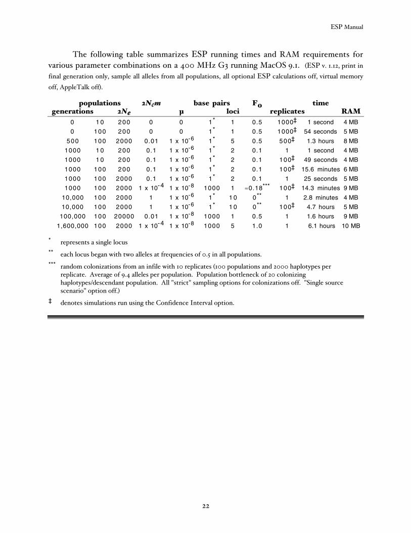
The following table summarizes ESP running times and RAM requirements forvarious parameter combinations on a 400 MHz G3 running MacOS 9.1. (ESP v. 1.12, print infinal generation only, sample all alleles from all populations, all optional ESP calculations off, virtual memoryoff, AppleTalk off).

populations 2Nem base pairs F0 timegenerations 2Ne µ loci replicates RAM

0 1 0 200 0 0 1* 1 0.5 1000‡ 1 second 4 MB

0 100 200 0 0 1* 1 0.5 1000‡ 54 seconds 5 MB

500 100 2000 0.01 1 x 10-6 1* 5 0.5 500‡ 1.3 hours 8 MB

1000 1 0 200 0.1 1 x 10-6 1* 2 0.1 1 1 second 4 MB

1000 1 0 200 0.1 1 x 10-6 1* 2 0.1 100‡ 49 seconds 4 MB

1000 100 200 0.1 1 x 10-6 1* 2 0.1 100‡ 15.6 minutes 6 MB

1000 100 2000 0.1 1 x 10-6 1* 2 0.1 1 25 seconds 5 MB

1000 100 2000 1 x 10-4 1 x 10-8 1000 1 ≈0.18*** 100‡ 14.3 minutes 9 MB

10,000 100 2000 1 1 x 10-6 1* 1 0 0** 1 2.8 minutes 4 MB

10,000 100 2000 1 1 x 10-6 1* 1 0 0** 100‡ 4.7 hours 5 MB

100,000 100 20000 0.01 1 x 10-8 1000 1 0.5 1 1.6 hours 9 MB

1,600,000 100 2000 1 x 10-4 1 x 10-8 1000 5 1.0 1 6.1 hours 10 MB

* represents a single locus** each locus began with two alleles at frequencies of 0.5 in all populations.*** random colonizations from an infile with 10 replicates (100 populations and 2000 haplotypes per

replicate. Average of 9.4 alleles per population. Population bottleneck of 20 colonizinghaplotypes/descendant population. All "strict" sampling options for colonizations off. "Single sourcescenario" option off.)

‡ denotes simulations run using the Confidence Interval option.

ESP Manual

23

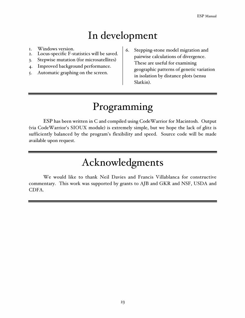
In development1. Windows version.2. Locus-specific F-statistics will be saved.3. Stepwise mutation (for microsatellites)4. Improved background performance.5. Automatic graphing on the screen.

6. Stepping-stone model migration andpairwise calculations of divergence.These are useful for examininggeographic patterns of genetic variationin isolation by distance plots (sensuSlatkin).

ProgrammingESP has been written in C and compiled using CodeWarrior for Macintosh. Output

(via CodeWarrior's SIOUX module) is extremely simple, but we hope the lack of glitz issufficiently balanced by the program's flexibility and speed. Source code will be madeavailable upon request.

AcknowledgmentsWe would like to thank Neil Davies and Francis Villablanca for constructive

commentary. This work was supported by grants to AJB and GKR and NSF, USDA andCDFA.

ESP Manual

24

Literature citedAvise, J. C. 1994. Molecular markers, natural history and evolution. Chapman and Hall,

New York, USA.

Bohonak, A. J. 1999. Dispersal, gene flow and population structure. Quarterly Review ofBiology 74: 21-45.

Bohonak, A. J., N. Davies, F. X. Villablanca, and G. K. Roderick. in press. Invasion geneticsof New World medflies: testing alternative colonization scenarios. BiologicalInvasions.

Cockerham, C. C., and B. S. Weir. 1987. Correlations, descent measures: drift withmigration and mutation. Proceedings of the National Academy of Sciences of theUnited States of America 84: 8512-8514.

Excoffier, L., P. E. Smouse, and J. M. Quattro. 1992. Analysis of molecular variance inferredfrom metric distances among DNA haplotypes: application to human mitochondrialDNA restriction data. Genetics 131: 479-491.

Hairston, N. G., Jr., L. J. Perry, A. J. Bohonak, M. Q. Fellows, C. M. Kearns, and D. R.Engstrom. 1999. Population biology of a failed invasion: paleolimnology of Daphniaexilis in upstate New York. Limnology and Oceanography 44: 477-486.

Hartl, D. L., and A. G. Clark. 1997. Principles of population genetics. 3rd edition. SinauerAssociates, Sunderland, MA, USA.

Maddison, D. R., D. L. Swofford, and W. P. Maddison. 1997. NEXUS: an extensible fileformat for systematic information. Systematic Biology 46: 590-621.

Miller, M. P. 1998. TFPGA: Tools for population genetic analyses for Windows. ArizonaState University, USA.

Page, R. D. M. 1996. TREEVIEW: An application to display phylogenetic trees on personalcomputers for Computer Applications in the Biosciences 12: 357-358., Macintosh.

Roderick, G. K. 1996. Geographic structure of insect populations: gene flow,phylogeography, and their uses. Annual Review of Entomology 41: 325-352.

Schneider, S., J.-M. Kueffer, D. Roessli, and L. Excoffier. 1998. Arlequin: a software forpopulation genetic data analysis for Windows. Geneva, Switzerland.

Slatkin, M. 1985. Gene flow in natural populations. Annual Review of Ecology andSystematics 16: 393-430.

Slatkin, M. 1994. Gene flow and population structure. Pages 3-17 in L. A. Real, editorEcological genetics. Princeton University Press, Princeton, NJ.

ESP Manual

25

Slatkin, M., and H. E. Arter. 1991. Spatial autocorrelation methods in population genetics.American Naturalist 138: 499-517.

Takahata, N., and M. Slatkin. 1984. Mitochondrial gene flow. Proceedings of the NationalAcademy of Sciences of the United States of America 81: 1764-7.

Wade, M. J., and D. E. McCauley. 1988. Extinction and recolonization: their effects on thegenetic differentiation of local populations. Evolution 42: 995-1005.

Weir, B. S. 1996. Intraspecific differentiation. Pages 385-405 in D. M. Hillis, C. Moritz andB. K. Mable, editors. Molecular systematics. Sinauer Associates, Sunderland, MA.

Weir, B. S., and C. C. Cockerham. 1984. Estimating F statistics for the analysis ofpopulation structure. Evolution 38: 1358-1370.

Wright, S. 1931. Evolution in Mendelian populations. Genetics 16: 97-159.