Everything for Filament Winding

Official Training Manual for McClean Anderson’s Composite Software Suite

Composite Designer – Pattern Entry Omniwind – Machine Operation

Contact Information: McClean Anderson 300 Ross Avenue Schofield, WI 54476-0020 USA

Phone: +1 (715) 355-3006 Fax: +1 (715) 359-0900

On the Web: www.mccleananderson.comEmail: sales@mccleananderson.com © 2004 McClean Anderson Inc., All Rights Reserved. All information contained in this document is believed accurate at the time of printing. All trademarks belong to their respective owners. Important note: this manual contains confidential technical information on McClean Anderson software and control systems and is only intended for use by McClean Anderson customers for the operation of our machines. Disclosure of this information to third parties is prohibited without express written consent from McClean Anderson.

Table of Contents 1. What is Filament Winding? .............................................................................................. 1 2. Some Filament Winding Basics........................................................................................ 3 3. Composite Designer Overview......................................................................................... 6 4. Installing and Starting-up Composite Designer................................................................ 8

4.1. Installation with hardware based protection key ...................................................... 8 4.2. Installation with software based protection key........................................................ 8 4.3. Additional configuration........................................................................................... 9

5. Introduction to Composite Designer Interface................................................................ 10 5.1. Toolbar Reference................................................................................................... 11 5.2. File Extension Reference ........................................................................................ 12

6. Helical Winds.................................................................................................................. 13 6.1. Defining the helical wind parameters ..................................................................... 13 6.2. Wind Pattern Selection ........................................................................................... 16

7. Circumferential Winds.................................................................................................... 20 8. Bottle Winds ................................................................................................................... 22

8.1. Defining the bottle wind parameters....................................................................... 22 8.2. Wind Pattern Selection ........................................................................................... 26

9. Zero Degree Winds ......................................................................................................... 30 10. Non-linear Winds........................................................................................................ 32

10.1. Mandrel Editing .................................................................................................. 35 10.2. Path selection ...................................................................................................... 37

11. Visual Rendering ........................................................................................................ 41 12. Motion Generation ...................................................................................................... 44

12.1. Machine Offsets – setting key reference locations ............................................. 45 12.2. Motion Generation Options – selecting axis behavior........................................ 46 12.3. Segment Flags – for file chaining ....................................................................... 47 12.4. Motion Generation Information – for tooling clearance..................................... 47 12.5. Machine Velocities – establishing the rate envelope.......................................... 49

13. Motion Editing ............................................................................................................ 52 13.1. Overview of motion generation process ............................................................. 52 13.2. Motion Editing, first steps................................................................................... 53 13.3. Additional Viewing and Editing Commands...................................................... 58 13.4. Direct Motion Generation ................................................................................... 63 13.5. Motion Table Editing.......................................................................................... 63 13.6. Spreadsheet Table Functionality......................................................................... 66 13.7. Inserting motion via the table ............................................................................. 68 13.8. Merging Motion Files and Manual Chaining...................................................... 70

14. Motion Filtering.......................................................................................................... 73 14.1. Initial Filter Parameter Entry .............................................................................. 73 14.2. Additional Filter Parameters ............................................................................... 78 14.3. Advanced Filter Parameters................................................................................ 80 14.4. Using Excel® to Graph and Compare Filtered Motion ...................................... 84 14.5. Chain File Filtering Issues .................................................................................. 86 14.6. Some Tips on Motion Smoothing ....................................................................... 87

15. Chain / Transition Files............................................................................................... 89

15.1. Transition Motion Files....................................................................................... 90 15.2. Transition Path Files ........................................................................................... 91 15.3. Do Not Transition option.................................................................................... 92 15.4. Chain File Tips and Troubleshooting ................................................................. 93

16. Auxiliary Output Files ................................................................................................ 94 16.1. Digital Auxiliary Outputs ................................................................................... 95 16.2. Analog Auxiliary Outputs................................................................................... 97 16.3. Use of Timers...................................................................................................... 98 16.4. Final notes on auxiliary outputs.......................................................................... 99

17. Omniwind ................................................................................................................. 101 17.1. Installation issues, startup, user accounts ......................................................... 101 17.2. Software/User Interface Overview ................................................................... 104 17.3. Initial Machine Motion ..................................................................................... 108 17.4. Loading and Executing Files ............................................................................ 111 17.5. Manual Operation/Jogging and Manual Offset................................................. 113 17.6. Use of Offsets ................................................................................................... 114 17.7. Shutting Down .................................................................................................. 115 17.8. Light Tower ...................................................................................................... 116 17.9. Additional Programming Features / Configuration .......................................... 116 17.10. Interfacing to Tensioner and Dr. Blade............................................................. 120 17.11. Troubleshooting ................................................................................................ 122 17.12. Advanced Troubleshooting............................................................................... 123

18. Digital Tensioning .................................................................................................... 129 18.1. Safety ................................................................................................................ 129 18.2. Tensioner Overview.......................................................................................... 130 18.3. Basic Tensioner Operation................................................................................ 132 18.4. Advanced Tensioner Controls........................................................................... 134 18.5. Automated Operation with Omniwind.............................................................. 136 18.6. Troubleshooting ................................................................................................ 137 18.7. Tensioner Command Table............................................................................... 139

19. Digital Dr. Blade....................................................................................................... 142 19.1. Basic Operation................................................................................................. 142 19.2. Dr. Blade Command List .................................................................................. 144 19.3. Gain Adjustment ............................................................................................... 144 19.4. Automated Operation with Omniwind.............................................................. 144 19.5. Trouble Shooting .............................................................................................. 145

20. Coordinator Software................................................................................................ 146 A. Verifying Part Coverage and Pattern Closure............................................................... 151

1. What is Filament Winding?

While the typical attendee of this course is already familiar with the concept of filament winding, a basic overview of the process can help to clarify the steps needed to take a product from conception to a fully functional parts program. In filament winding, a machine, rather like a lathe, spins a mandrel. In synchronization with this, the machine moves one or more additional axes in order to wind a composite material such as a fiberglass, carbon fiber, or Kevlar over the surface of this mandrel in a very precise, controlled manner. The material can be dry wound, a prepreg or run through a resin bath for wet winding applications. Once the desired number of layers have been laid on the mandrel, the part is cured and depending on the process, the mandrel either becomes part of the final product (such as plastic water tanks) or is removed – generally using force or by chemical or physical destruction of the mandrel. Unlike typical machining (e.g. milling, lathing…), the motion of the machine itself does not directly correspond e

gta IdbAm

Figure 1 – a filament wound bottl

to part being produced. Instead, a fiber payout system

guides the fiber while moving at some clearance from the mandrel surface. Tension in the system naturally causes the fiber to assume a tangential path from a contact point on the surface of the part to a contact point in the payout system. When this tension is exactly along the current position and orientation of the fiber at the surface of the part (i.e. longitudinal or fiber-axial force), then the machine is performing a

eodesic wind. Imagine putting a string on the surface of a globe – if the string is pulled ight, the tension will also cause it to follow this same geodesic path – it is the shortest path cross the surface of a convex curve.

n real filament winding, the desired fiber weave is rarely geodesic, so the path must be eflected from a pure geodesic one. These lateral forces require some degree of friction etween the fiber and the surface of the mandrel or part, otherwise the fiber will slip. lternatively, additional devices such as pin-rings can be mounted on the surface of the andrel to assist with fiber-guidance and control slippage. This is one of the key issues to be

considered when creating a filament wound part – in essence can this part be filament wound?

1

That question does not have a simple answer – although there are many practical experiences which show that fairly complex parts can be successfully wound. In addition to the mandrel surface, the designer should also consider the effects of wind angle and resulting pattern when considering if a part can be wound. In general, parts / patterns with the following traits are easily wound:

- Symmetrical about an axis of rotation (which would become the mandrel axis). In many cases, asymmetrical parts can also be wound, although they may require significantly more complex programming.

- Convex surface curvature (note that only the curvature seen by the fiber is relevant, a curve which is concave when examined from a particular fiber angle may disappear or become convex at a different angle). Fibers will naturally bridge concave curves.

- No abrupt changes in angle – these tend to lead towards fiber slippages – an alternative is to use pin-rings.

The vast majority of filament wound parts are variations of cylinders, domes, and cones, and occasionally other 3-D projections of simple 2-D surfaces such as squares or other polygons. In some cases, more complex, asymmetrical 2-D surfaces are projected along a 3rd axis and wound such as helicopter blades. Finally, with very sophisticated control, non-axisymmetric parts can also be wound such as elbows and T-junctions, although at present, Composite Designer does not support such designs.

2

2. Some Filament Winding Basics In this course, we will cover the capabilities of Composite Designer for generating a wide variety of parts programs. To begin, here is a picture showing the basic components of a filament winder in operation.

Figure 2 – Picture of filament winder in operation. The large yellow cabinet is a tensioning system which moves in tandem with the carriage.

The machine and mandrel are fairly obvious components. On the left side is the operator panel. Behind the machine is a fiber tensioning system or simply a tensioner. For less demanding applications, various friction-based systems (possibly as simple as winding the fiber through multiple eyelets) are used instead to increase tension. In general, multiple fiber tows will be fed off of fiber creels, flow through various guides, through a resin dispenser (if wet-winding; generally a resin bath or drum), and out of a payout system (generally one or more fiber combs and a D-ring or rollers) onto the mandrel itself. This group of fibers together forms one fiber bandwidth. Note that effective bandwidth often varies from the sum of the nominal fiber bandwidths, and that this further varies depending on the fiber payout system, the fiber angle and the radius of curvature of the mandrel (the lower the angle and the smaller the part radius, the smaller the effective bandwidth as the fibers tend to bunch up). Often, the designer will need to actually measure the resulting bandwidth and use this in a further design iteration when generating a parts program – particularly if it is critical for a pattern to “close”. A “closed” pattern will completely cover a mandrel, leaving no gaps between fibers. The machine operator may also

3

adjust aspects of the payout system such as the placement and routing of fibers through fiber combs.

Figure 3 – Simple representation of fiber bandwidth

Figure 4 – Definition of fiber bandwidth on surface of mandrel

Already “fiber angle” has been mentioned several times – this is the angle between the fiber’s orientation at the surface of the mandrel and an intersecting surface line that is parallel to the mandrel’s axis of rotation. By this convention, a “low-angle wind” is one which approaches the mandrel axis (if the mandrel were a globe, a zero-angle wind would be from pole-to-pole – parallel to lines of longitude – and is therefore also called a polar wind). A “high-angle wind” is one which approaches the perpendicular of the mandrel axis and winds the mandrel like a spool (returning to the globe example, a 90-deg angle wind would be like wrapping around the equator, or parallel to lines of latitude). Figure 6 makes this point.

4

Figure 5 – Definition of fiber angle

Figure 6 – examples of high- and low-angle winds. The high-angle wind is on the left.

The basic design parameters of bandwidth and fiber angle will appear again and again when generating a filament wound part.

5

3. Composite Designer Overview When generating Composite Designer part programs, users tend to follow the same basic sequence of steps:

Step 1: Select appropriate mandrel geometry. At present, Composite Designer supports the following geometry types: A circumferential wind is a near-90-deg wind where for every revolution of the mandrel, the carriage advances along the mandrel axis by one bandwidth, essentially wrapping the mandrel. In a helical wind, the carriage moves at a much higher rate, with controlled acceleration, deceleration, and fixed velocity sections to obtain various helical patterns on the surface of the mandrel. The helical and circumferential winds are commonly used for pipes/cylinders and other 3-D projections of 2-D surfaces. In a bottle wind, a dome is added to both ends of the mandrel and the axes combine to form much more complex motion as the fiber is laid at a particular angle over the cylindrical bottle section and then changes into an appropriate near-geodesic path over the domes. A non-linear wind allows for a much greater degree of flexibility by allowing the designer to specify essentially any longitudinal mandrel profile, which is then revolved around the mandrel’s axis to form the 3-D mandrel (i.e. it specifies radius against position along mandrel axis). Furthermore, the designer can specify different wind angles at different positions along the axis. Of course, as has been mentioned, not all profiles and fiber angles are well suited to being wound. A chain-wind is formed by combining any of the above winds into a single motion program – this is useful to increase machine productivity and in many cases, to provide a smooth fiber path to transition from one segment to the next. A zero-degree wind is somewhat unique in that it directly specifies machine motion rather than part geometry. It is used for specialized applications in which a true-zero degree fiber angle is required.

Step 2: Enter basic part information. This will vary from part geometry to part geometry and is covered in the subsequent sections. This also includes basic wind parameters such as bandwidth and fiber angle.

Step 3: Use this information to generate a fiber path. Once Composite Designer is given all the necessary information, it will use this to generate a listing of paths that correspond to the given inputs. These paths will vary by minor differences in the input parameters, which will result in different wind patterns and other physical wind characteristics. The user can study and sort these various possible paths and select the path he/she feels will best match the design at hand. In some cases, the user will need to iterate this and try the following steps several times to establish a stable or more optimal path.

6

Step 4: Examine the resulting path. Composite Designer includes powerful 3-D parts rendering to assist the user in visualizing the final part.

Step 5: Enter machine motion parameters. Here the user will establish the desired clearances the machine should maintain from the surface of the part, along with determining various types of envelopes to control machine motion.

Steps 6 and 7: Examine and tweak the resulting motion. Particularly with complex parts such as bottles, the resulting motion may require some user-assisted post-processing to improve machine performance and smooth any spikes in machine motion. Execute the program. In some cases, this may be done prior to any motion post-processing since the user may first wish to establish if a particular path is stable. As mentioned above, the user may need to perform a few design iterations between steps 3 and 7 (and possibly 2). Also, generating chain files is a somewhat more complex sequence of events involving generating and testing individual segments and then combining these and performing some additional tweaking. Once these steps have been completed, the designer should have a viable parts program, which is well suited to generating the desired component. As the designer gains experience, the process will become more rapid and he/she will gain insight into critical design parameters and often be able to quickly form judgments ranging from determining if a part is well suited to filament winding, to selecting the appropriate wind parameters. In the subsequent sections, we will cover the generation of each category of Composite Designer parts programs. A few formatting notes of this manual:

- Filename extensions are shown in italics: mct, hlx, etc. - Menu navigation is shown in Arial with menu layers indicated by a vertical bar:

File | Open… indicates the user should use the mouse to click on the File menu heading and then the Open… submenu heading.

7

4. Installing and Starting-up Composite Designer For regular users, starting up Composite Designer (from here on labeled CD) is as simple as clicking on its icon. However, first time users and those in special circumstances need to be aware of program installation and configuration.

4.1. Installation with hardware based protection key The latest version of CD uses a hardware based software protection key to prevent unauthorized program distribution (also known as a “dongle”). Two different key versions are available – one for the printer/parallel port (which includes a “pass through” port for printing), and one for the USB port. They implement the same function and are interchangeable. Installing the software requires the user to log into the given computer with administrator privileges (for network operating systems such as Windows ® NT, 2000, or XP). Make sure that no hardware key is installed. Then use a program like Windows Explorer to navigate to the appropriate installation program (generally the file path is something like: “\\Composite Designer X.X\Disk1\Setup.exe” – where \\ is the location/letter of the drive and X.X is the current version number). The setup program is very similar to most Windows® installation software. Note that the installation package will install both Composite Designer and the drivers for the hardware key (from Rainbow® technologies). When upgrading, it is recommended that both Composite Designer and the hardware key drivers be uninstalled before upgrading to the newer version (using the standard Windows uninstall methods). Before running the software for the first time, remember to plug in the hardware key.

4.2. Installation with software based protection key Earlier versions of CD use a software based protection key. Installation is similar to the method described above (again, the installation should be done via an administrator account). During installation, the user will be requested to enter a machine number – this should have the format: X###### - there X is a letter, typically J for job number, and # is a numeral. The first 4 digits of this number are the machine’s serial number while the last 2 digits are used to describe the current software version (e.g. J123412 would be machine #1234 with software version 1.2). The actual number entered – particularly the version number – is not absolutely critical, although it will assist McClean Anderson staff when registering the software. When CD is run for the first time, a registration screen appears asking the user to enter a software registration key. Users should contact McClean Anderson to obtain this key. Note that the software should also be run with administrator privileges when entering this software key as well. Once the software is unlocked, any user of the PC can run it. As with the hardware key version, users are requested to uninstall previous versions before installing newer ones.

8

4.3. Additional configuration Before CD can generate machine motion programs, it needs to obtain the parameters of the machine that will execute the program. These are stored in .mct files. Each machine built is given a specific mct file, which is given the name of the machine’s serial number (e.g. “j1234.mct”). When executing CD for the first time, or in a facility which has different types of McClean Anderson winders, users need to select the machine for which they wish to produce motion. This choice remains until a new mct file is selected. To select an mct file, use the menu entry: Options | Current MCT File… This will bring the user to a file dialog box where they can select an appropriate mct file.

9

5. Introduction to Composite Designer Interface Composite Designer (CD) has a user interface, which should be familiar to users of Windows applications. Program control is provided through a set of menus and quick access to specific tasks is achieved through use of a toolbar and, in some cases, keyboard commands. Figure 7 is a picture of CD displaying various aspects of parts programming.

Figure 7 - Typical Composite Designer Screen. At top, the menu bar and tool bar are visible. In the main window, the following windows related to a particular bottle wind are shown clockwise from top left: Winding parameter dialog box, Motion graph, Wind pattern selection dialog, and 3-D rendering of wound bottle.

These individual windows will be covered in subsequent sections. The menus and toolbars are largely fixed, although items become enabled and disabled based on the active window. Some buttons, such as file access, are generally available while some are specific to various portions of the editing process. The following reference of toolbar functions is taken from the CD help file and can be referred back to when covering other portions of this training. It is followed by a reference of the various file extensions (suffixes) generated and used by CD.

10

5.1. Toolbar Reference The Toolbar is a row of buttons at the top of the main window that represent Composite Designer application commands. Clicking one of the buttons is a quick alternative to choosing a command from the menu. Buttons on the toolbar activate and deactivate according to the state of the application. The toolbar itself may be moved with the mouse and left as a floating palette, or docked to any edge of the main window. Button Action Menu Equivalent

Create a new wind module File | New

Locate and open a wind module File | Open

Save the current wind module File | Save

Cut selected text to clipboard

Copy selected text or current view to Clipboard

Paste text from Clipboard

Reject current edit operation Calculate | Discard New Dataset

Accept current edit operation Calculate | Accept New Dataset

Terminate the current fiber rendering

View | Stop Fiber Plot

Enable mouse pointer to select zoom range

View | Zoom Menu | Zoom Window

Show previous zoom window View | Zoom Menu | Zoom Previous

Show full dataset View | Zoom Menu | Zoom All

Scroll zoomed window left 10% View | Zoom Menu | Scroll Left

Scroll zoomed window right 10% View | Zoom Menu | Scroll Right

Set mouse pointer to insert data points

Calculate | Insert Points

Delete selected dataset range Calculate | Add Points

Display help file contents Help | Contents

Table 1 – description of toolbar buttons

11

5.2. File Extension Reference Composite Designer generates and uses quite a few different files. This is a brief synopsis of each file extension: Extension Description

.ang an angle definition file, used to establish fiber angle and/or wind start and end points for non-linear winds

.aux an auxiliary output file, used to control Omniwind in tandem with a motion file to define conditions for controlling auxiliary outputs

.bld a compiled Dr. Blade control file – generated by Coordinator .btl a bottle wind parameter file .chn a chained motion file, consisting of more than one segment (i.e. several

.mmt files chained together to allow the machine operator to lay down multiple layers in a single sequence)

.cir a circumferential wind parameter file

.cts a chained segment file used by the older Compositrak series machines .ctw a chain transition wind used to chain multiple parameter files together to

produce a chained path-based or motion-based compound motion file .gen a general wind parameter file, used to store the parameters of a non-

linear wind .hlx a helical wind parameter file .mct a machine configuration file. mct files are provided by McClean Anderson

for each built machine and used by CD to obtain information on the machine to be controlled

.mdf a mandrel definition file, generated any time a fiber path is created; describes the geometry of the given mandrel; useful as a starting point for non-linear winds

.mfp motion filter parameters – keeps track of filtering parameters corresponding to current motion file

.mmt a simple machine motion file, consisting of only one segment .pth a path file; essentially a list of sequential coordinates describing a single

circuit of fiber path across the surface of a mandrel; used when generating motion and for 3D rendering purposes

.seg a segment motion file used by the Compositrak series machines; not specifically covered in this guide.

.ten a compiled digital tensioner control file – generated by Coordinator

.tre a raw text tensioner or Dr. Blade control file – generated by Coordinator .zro a zero degree wind parameter file

Table 2 – listing of file extensions used and/or created by Composite Designer

Note: parameter files (e.g. hlx) contain the initial parameters entered by the user but no solution information such as a fiber path, mandrel definition, or machine motion, hence they are very compact.

12

6. Helical Winds In this section, we will cover the first steps of generating a helical part – one of the most common types of filament windings. Subsequent sections will cover the steps for generating other part shapes as well as motion generation and machine control. Once Composite Designer (CD) is opened and properly initialized as described in previous sections, the user can begin parts entry.

6.1. Defining the helical wind parameters To begin programming a new part, simply select the File | New menu option (or the toolbar button). This brings up a pop-up menu allowing the user to decide which type of file they wish to create. We will select Helical Wind from the pop-up menu. This brings up the following dialog box:

Figure 8 - Helical wind parameter dialog box.

This dialog box allows the user to specify the various relevant parameters for the wind. Each parameter is covered in turn in the following paragraphs. The first two parameters (Fiber Start Position and Fiber End Position) describe the location at which the Helical fiber path begins and ends. Note - these locations are relative to the Mandrel Origin, are not bandwidth compensated (i.e. they describe the fiber center line), and may be located at any position along the mandrel. Figure 9 shows these key mandrel locations. Also, the wind may begin at either end of the mandrel. If the fiber start position has a larger value than fiber end, then the wind would begin at the far side of the mandrel, away from the headstock. However, the recommended way to reverse the wind is during path selection (after pressing the Calculate button – see page 19).

13

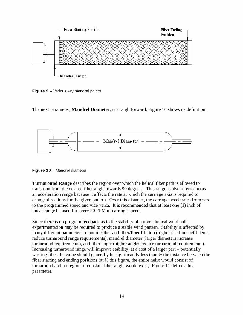
Figure 9 – Various key mandrel points

The next parameter, Mandrel Diameter, is straightforward. Figure 10 shows its definition.

Figure 10 – Mandrel diameter

Turnaround Range describes the region over which the helical fiber path is allowed to transition from the desired fiber angle towards 90 degrees. This range is also referred to as an acceleration range because it affects the rate at which the carriage axis is required to change directions for the given pattern. Over this distance, the carriage accelerates from zero to the programmed speed and vice versa. It is recommended that at least one (1) inch of linear range be used for every 20 FPM of carriage speed. Since there is no program feedback as to the stability of a given helical wind path, experimentation may be required to produce a stable wind pattern. Stability is affected by many different parameters: mandrel/fiber and fiber/fiber friction (higher friction coefficients reduce turnaround range requirements), mandrel diameter (larger diameters increase turnaround requirements), and fiber angle (higher angles reduce turnaround requirements). Increasing turnaround range will improve stability, at a cost of a larger part – potentially wasting fiber. Its value should generally be significantly less than ½ the distance between the fiber starting and ending positions (at ½ this figure, the entire helix would consist of turnaround and no region of constant fiber angle would exist). Figure 11 defines this parameter.

14

Figure 11 – shows the definition of turnaround range on a typical helical mandrel.

The next parameters to be specified are Fiber Angle and Fiber Bandwidth. These parameters were defined in section 2. In general, the larger the bandwidth, the faster the part is completed (fewer strokes are required). Fiber angle is one of the critical design parameters of any composite part. Unlike metals and other homogenous substances, the characteristics of composite materials are not the same in all orientations – generally, they exhibit much higher strengths in the directions of fibers. Hence a high-pressure cylinder would generally want a high-angle wind since this effectively aligns the fibers against pressure forces, while a structural post would typically be at a much lower angle for effective strength against bending. These basic concepts only scratch the surface of composite engineering. A detailed analysis on how to select wind angles and similar parameters is far beyond the scope of this booklet. The reader is advised to consult composite literature1. End Dwell describes the number of degrees of mandrel rotation while the carriage waits at the end of a stroke. In a single stroke, the carriage accelerates to attain the selected fiber angle, maintains constant velocity while depositing fiber at the selected angle, decelerates to zero velocity, and then maintains constant position while the mandrel continues to rotate through this end dwell parameter, before starting the return trip to the opposite end of the part. In many respects, end dwell complements turnaround range – they both affect how stable a path is likely to be. It also affects the precise length of the part. This has to do with the approximation made on helical winds. The following aside is not critical to making parts programs or understanding CD, but it offers some insight into the differences between fiber path and machine motion: (also see chapter on chain winds as there are some minor differences in motion calculation between simple helixes and chained helixes).

Unless the user is chaining several helixes together, the actual motion executed in a helical wind is an approximation of the true helix. In many cases, the difference is unlikely to be noticed, although for particularly low wind angles with little end dwell, the user may note that the resulting part is slightly shorter than anticipated. This has to do with the translation between fiber path and machine motion. On a simple helix, the carriage actually follows the motion as described above (accelerate,

1 For a much more thorough discussion of filament winding, see “Filament Winding Composite Structure Fabrication” by S.T. Peters, W.D. Humphrey, and R.F. Floral. Published by SAMPE Publications. Currently in its second edition.

15

constant velocity, decelerate, dwell), but this motion is not entirely accurate in terms of guiding the fiber at the correct tangential. The correct motion would have the carriage overshoot both ends of the part and then retract in order to ensure that the wind successfully reaches the end points. Imagine if the turnaround range were set very small – essentially zero - and the wind angle were low. When the carriage reached its end of travel, the fiber angle would still be at this low angle and would gradually approach 90deg. as the machine moves through this end dwell. If the end dwell is set too short, then the fiber will not actually reach the end point before the carriage reverses direction, yielding a shorter than anticipated part. When CD chains several helical segments together, it no longer attempts to apply this simplification, hence the resulting motion is technically more accurate, but also less smooth.

Note that in an actual wind, fiber angle, fiber bandwidth, and particularly end dwell are all adjusted from their entered values to obtain a fiber path solution which will generate a particular wind pattern and, once the machine has completed a full cycle, places the payout eye in the exact same position as at program start. The final number to be entered is the Path Threshold parameter. This parameter establishes how often the software generates path coordinates. CD will calculate a path point for this increment of mandrel rotation. This can become quite obvious when generating a 3D rendering of the part. Because of the simplification mentioned in the aside above, this parameter is irrelevant in terms of generating machine motion for simple files, but it is used when chaining files together (where the simplification is not applied). For beginning users, this parameter rarely requires adjustment on helical winds (a default value of 5 degrees is generally acceptable, with values as high as 30degrees still reasonable). Finally, at the bottom of the dialog box is a check-box which allows the user to switch between metric and standard units of measurement. When the users checks this box, all linear measurements are taken in mm, otherwise they are in inches. Note that checking the box does not rescale any numbers to reflect the switch to metric/standard units. Also, in both measurement systems, angles are given in degrees. At this point, the user has completed the initial entry of wind parameters and he/she may press the calculate button in the dialog box.

6.2. Wind Pattern Selection Assuming the exact parameters shown in the previous section were entered, once the user pressed the Calculate button, the following path selection dialog box would appear:

16

Figure 12 – Wind Pattern Selection dialog box

In this case, the user is presented with the first 9 of 18 possible winds (the total number is displayed on the first line of the dialog box). The scrollbar is used to display the rest. By default, the display is sorted by Natural Path Deviation (which is proportional to the deviation from the desired angle). By using the “Sort” button at the bottom of the box, the user can choose a different sort criterion, which is quite useful in cases which generate large numbers of entries. The other entries at the top of the screen indicate mandrel rotation for a complete circuit (distance covered in the time it takes the carriage to traverse from start to end and back to the start again) and also the mandrel rotation in the turnaround range (while the carriage decelerates, dwells, and accelerates in the opposite direction). These data values are only generated for the first path shown. The user may now select which wind pattern they wish to convert into motion. They may use the 3D rendering functions to assist with this selection (see chapter 11). Going through the columns one by one: Circuits/Coverage indicates the number of carriage circuits (from starting point to end point and back again) needed to close the pattern. Recall that a closed pattern is when the fiber covers the entire surface of the mandrel (and requires that the entered bandwidth match the actual bandwidth). In almost all cases, the software will generate solutions which differ by 1 circuit count and which adjust the calculated bandwidth to be slightly higher and lower than the entered bandwidth.

17

Pattern indicates the type of pattern the user will obtain. Larger numbers indicate a tighter weave (which also tends to lead to a greater buildup of thickness and hence voids in the composite structure), while low numbers have less fiber interweaving. This number can be established by examining a mandrel. Beginning at the corner of a diamond pattern and following a circumferential route around the mandrel, count the number of diamonds that appear on the surface of the part. Figure 13 shows a 2-pattern weave:

Figure 13 – shows a 2-pattern weave – each diamond occupies 180deg. of mandrel revolution and a second diamond would appear on the side facing away from the observer.

Pattern is again an important parameter for a filament wound part, involving various tradeoffs in the final product. Precise pattern selection is beyond the scope of this document. Pattern Type: Lead/Lag – patterns have two possible ways to build up on the mandrel. After the machine completes the pattern number of circuits (e.g. after 3 cycles on a 3-pattern wind), the next circuit will place fiber directly next to the original circuit. Leading or lagging describes on which side of the original fiber later circuits will be placed. On a lead pattern, newer circuits are placed ahead of older ones in the direction of rotation (i.e. they come into view first as the mandrel rotates). On lagging patterns, they are placed behind older ones. Figure 14 describes this effect. Lead/lag selection may have some effect on path stability.

18

Figure 14 – shows the difference between fiber build-up with a leading and a lagging pattern.

Natural Path Deviation: This column indicates a relative deviation between the natural, or base fiber path and the adjusted fiber path required for this pattern. In essence, this number represents the degree to which the user specified entries were adjusted in order to obtain a pattern which closes properly. Besides selecting a particular path, the user can also decide it the wind should start on the left (headstock) or right side of the mandrel. Clicking the option “Start on Right End of Mandrel” will reverse the normal path (and motion) of the wind. This is often useful when winding multiple programs (or a chain file), one of which is a circumferential wind. Circumferential winds with an odd number of layers leave the carriage at the opposite end of the machine. Once the user has selected an appropriate pattern, he/she may click “OK” and a new dialog box will appear requesting the user to save the file (clicking “Cancel” will return the user to the previous, parameter-entry dialog box). Helix files are saved with the extension .hlx. A path file (.pth) and a mandrel definition file (.mdf) with the same name are also saved (see section 5.2). To complete the process of generating a helical part, the user would now typically render the generated path (turn to chapter 11), generate motion (chapter 12), evaluate and edit motion (chapter 13), and finally execute the program on the machine using Omniwind (chapter 17). The following chapters cover the basics of each different part geometry.

19

7. Circumferential Winds This chapter covers what are probably the simplest types of wind – the circumferential wrap or “hoop wind”. This wind largely consists of the mandrel rotating at a fairly high speed while the carriage moves over by one bandwidth for each mandrel revolution. Many concepts are identical to the helical wind. To begin, the user can click on the new part toolbar button:

and select Circumferential Wind from the pop-up menu. This brings up the following dialog box:

Figure 15 – The circumferential wind dialog box.

Going through the parameters one by one: Fiber Starting Position (Z1) establishes the carriage location where the machine will begin the program. The Dwell column establishes how many degrees the mandrel should rotate before the carriage begins to move. Generally, for a complete wrap this would be set to 360. Fiber Ending Position (Z2) establishes the carriage location where the machine will begin the program. Again, the user can enter a dwell. Mandrel Diameter and Fiber Bandwidth are fairly self-explanatory. Also, the mandrel figures from chapter 6 should clarify and bandwidth was defined in section 2 (see page 3). Coverage Strokes is unique to circumferential winds. Unlike other winds, circumferential motion is defined as strokes rather than circuits. A stroke is a single motion of the carriage towards either the headstock or the tailstock. If an even number of strokes is defined, the result is cyclic. With odd numbers, the machine (i.e. the carriage) ends up at a different location at the end of the wind. This can be useful for moving the machine a certain distance between layers (often with the bandwidth set very large). More detailed information about the stroke/circuit differences is available in section 13.5. Metric Units (mm) – if checked, all linear dimensions are considered to be millimeters. A few things to note: the wind can start at either end of the mandrel (i.e. if Z1 is greater than Z2, the wind will start near the tailstock and move towards the headstock). Also, the resulting motion is based on the fiber centerline and not bandwidth compensated, meaning the final wrap will be approximately 1 fiber bandwidth wider than entered. Finally, the given dwells

20

are applied at the end of every stroke. For example, if the user has the starting (Z1)-dwell set to 360 and the ending (Z2)-dwell set to 180, and the number of strokes is 2, then the machine will dwell 360, move from Z1 to Z2, dwell 180 then dwell 360, move from Z2 to Z1, dwell 180, and then stop. If other dwell characteristics are desired, these could be generated via chaining circ winds together. Once the parameters have been entered, the user can press Calculate to continue the process. With circumferential winds, there is only one solution to the entered parameters, so no additional user selection is required. The computer simply states that the path has been generated and then asks the user for a filename. The computer will now generate the circumferential wind file (.cir), a path file (.pth), and a mandrel definition file (.mdf – see section 5.2). At this point, the user can render the part to examine the wind (see chapter 11) and then proceed to generate machine motion (chapter 12).

21

8. Bottle Winds While simpler machines do a fair job at winding helixes and hoops, the use of multi-axis machines and sophisticated controls becomes very noticeable when generating bottle winds and other complex parts. They provide for excellent fiber control around the poles of the bottle, making program generation much easier and often greatly improving fiber stability.

8.1. Defining the bottle wind parameters The first step for generating a bottle wind is to begin a new part (via File | New or the toolbar button). This brings up another menu where the user can select Bottle Wind. This brings up the following dialog box:

Figure 16 – the bottle wind dialog box

The Bottle Wind module handles two types of bottle dome shapes, Ellipsoidal and Isotensoid. Both bottles have a cylindrical section and domes on both ends. The ellipsoidal dome, when cut along the mandrel axis, has an elliptical shape for its domes while the isotensoid dome consists of two 90-degree circular arc segments and a flat end to connect the two. Figure 17 shows examples of the two bottle shapes. In general, ellipsoidal shapes tend to generate better machine motion because they have fewer discontinuities. Often, bottles with an isotensoid shape are more easily wound using an ellipsoidal approximation (this is discussed in greater detail below). The dialog box has four tabs along the bottom of the parameters. In addition to the two shapes already discussed, the user can also select planar winds for each shape. With planar winds, the machine will try to wind from pole to pole and the fiber angle is automatically adjusted to near zero.

22

Figure 17 – Shows the difference isotensoid bottle shape (top) and ellipsoidal bottle shape (bottom). This particular ellipsoidal bottle has a width greater than ½ its diameter, giving a “pointy”, bullet-like dome.

The following covers the various parameters which determine the bottle wind: Mandrel Diameter – is fairly self-explanatory. Figure 18 gives a visual definition. Cylinder Length – this is the length of the cylindrical section of the bottle (not including the dome ends. Figure 18 gives a visual definition.

Figure 18 – Definition of Cylinder Length and Mandrel Diameter

For ellipsoidal bottles, the next two parameters are Left- and Right Dome Width. Together with the mandrel diameter, these determine the shape of the ellipse. Figure 19 gives a visual definition of the left (headstock side) dome width. If the dome width is set to the mandrel

23

radius (i.e. ½ of Mandrel Diameter), then the domes become spherical. Smaller values give flat domes while larger values give pointy ones.

Figure 19 – definition of Left Dome Width and Right Dome Width. These only apply to ellipsoidal bottles.

For isotensoid bottles, Left- and Right Dome Polar Opening replace dome width. These define the diameter of the flat ends of the isotensoid shape. Figure 20 gives a visual definition. As the polar opening approaches zero, the end becomes spherical; as it approaches the mandrel diameter, the end becomes cylindrical.

Figure 20 – definition of the Left Polar Diameter and Right Polar Diameter. These only apply to isotensoid bottles.

The Dome Evaluation Points parameter establishes how many sample points are taken to describe the profile of the dome on both ends of the mandrel. This affects how accurately the part will be calculated in software and the accuracy of path and consequently the rendered part and motion. In general, a value around 50 will produce good results and does not require further adjustment. Common to most dialog boxes, the user can select the measurement system. If the Metric (mm) box is checked, linear units are in millimeters. Otherwise they are in inches.

24

Fiber Angle and Fiber Bandwidth are common to almost all winds and have already been described in some detail. See pages 3 - 5 for more details and figures. The Left- and Right Polar Opening (Dia.) parameters define the desired opening in the fibers at the ends of the part. Figure 21 gives a visual definition. This parameter usually requires some adjustment to achieve a stable (i.e. small dome slip factor) wind. The appropriate value will first depend on the physical layout of the mandrel (e.g. the machine obviously can’t wind through any shaft protruding from the ends). Beyond this, the user may need to decide on the appropriate trade-offs between polar opening, fiber angle, and fiber stability. The user can obtain an approximate measure of path stability by examining the dome slip factors during path selection. If the left and right openings are significantly different in size, this can pose a problem to stability. In such cases, the user may wish to examine a non-linear wind (see chapter 10, especially page 39), which allows for a gradual change in fiber angle along the cylinder. The following section also covers topics of path stability in greater detail. Note: this parameter takes fiber bandwidth into account (i.e. it is not based on the fiber center line), so the desired opening value should be used.

Figure 21 – shows the definition of the Left Polar Opening and Right Polar Opening parameters. The figure on the left has less than 180 degrees of rotation as can be seen by comparing fiber entry and exit points across the pole. Depending on various external factors, this path may exhibit a tendency to fall off the part. The right dome has the opposite problem – over 180 degrees of rotation with a tendency to wrap around the pole. This shows the problems with having significantly different polar openings on the same bottle.

25

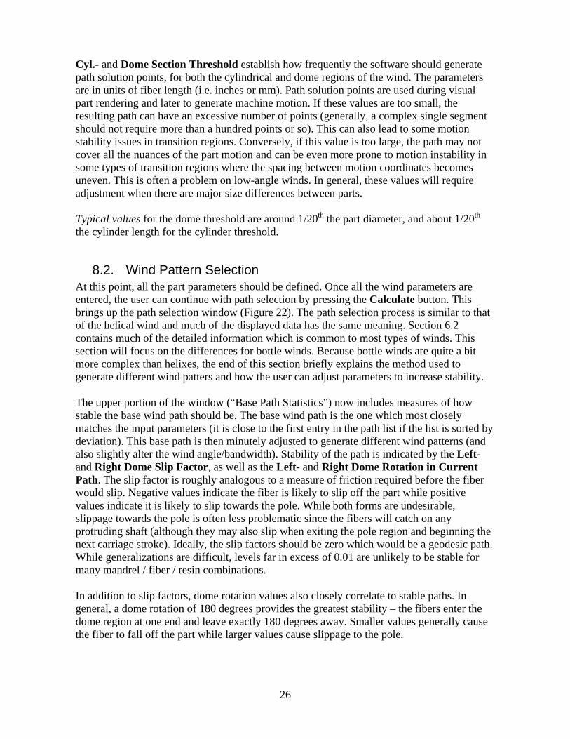
Cyl.- and Dome Section Threshold establish how frequently the software should generate path solution points, for both the cylindrical and dome regions of the wind. The parameters are in units of fiber length (i.e. inches or mm). Path solution points are used during visual part rendering and later to generate machine motion. If these values are too small, the resulting path can have an excessive number of points (generally, a complex single segment should not require more than a hundred points or so). This can also lead to some motion stability issues in transition regions. Conversely, if this value is too large, the path may not cover all the nuances of the part motion and can be even more prone to motion instability in some types of transition regions where the spacing between motion coordinates becomes uneven. This is often a problem on low-angle winds. In general, these values will require adjustment when there are major size differences between parts. Typical values for the dome threshold are around 1/20th the part diameter, and about 1/20th the cylinder length for the cylinder threshold.

8.2. Wind Pattern Selection At this point, all the part parameters should be defined. Once all the wind parameters are entered, the user can continue with path selection by pressing the Calculate button. This brings up the path selection window (Figure 22). The path selection process is similar to that of the helical wind and much of the displayed data has the same meaning. Section 6.2 contains much of the detailed information which is common to most types of winds. This section will focus on the differences for bottle winds. Because bottle winds are quite a bit more complex than helixes, the end of this section briefly explains the method used to generate different wind patters and how the user can adjust parameters to increase stability. The upper portion of the window (“Base Path Statistics”) now includes measures of how stable the base wind path should be. The base wind path is the one which most closely matches the input parameters (it is close to the first entry in the path list if the list is sorted by deviation). This base path is then minutely adjusted to generate different wind patterns (and also slightly alter the wind angle/bandwidth). Stability of the path is indicated by the Left- and Right Dome Slip Factor, as well as the Left- and Right Dome Rotation in Current Path. The slip factor is roughly analogous to a measure of friction required before the fiber would slip. Negative values indicate the fiber is likely to slip off the part while positive values indicate it is likely to slip towards the pole. While both forms are undesirable, slippage towards the pole is often less problematic since the fibers will catch on any protruding shaft (although they may also slip when exiting the pole region and beginning the next carriage stroke). Ideally, the slip factors should be zero which would be a geodesic path. While generalizations are difficult, levels far in excess of 0.01 are unlikely to be stable for many mandrel / fiber / resin combinations. In addition to slip factors, dome rotation values also closely correlate to stable paths. In general, a dome rotation of 180 degrees provides the greatest stability – the fibers enter the dome region at one end and leave exactly 180 degrees away. Smaller values generally cause the fiber to fall off the part while larger values cause slippage to the pole.

26

The remaining entry displayed at the top of the screen is Mandrel Rotation in Current Path. This is the mandrel distance covered during a complete circuit – including the cylindrical portion of the wind and the rotation in both domes. As with the helical wind, many different wind permutations are displayed below the base path. In this example, 9 of 58 generated winds are displayed and the scrollbar is used to display the rest. The same sorting criteria used for helical paths may be used for bottles.

Figure 22 - Wind Pattern Selection dialog box for bottles

The user may now select which wind pattern they wish to convert into motion by selecting a line in the path list box and clicking OK (or double-clicking on a line). 3-D part rendering can assist with this process (see chapter 11). The individual columns of the path selection list are all very similar to the parameters generated for helical winds (see pages 17 - 19). Looking at each in turn: Circuits/Coverage indicates the number of carriage circuits (from starting point to end point and back again) needed to close the pattern. Pattern indicates the type of pattern the user will obtain. Larger numbers indicate a tighter weave. The same method as with the helix can be used to determine a bottle’s pattern number. With the bottle, an alternate method is to count the number of points on the star-like patterns which form at the poles. Figure 21 shows a 7-pattern weave.

27

Pattern Type: Lead/Lag – Leading or lagging describes on which side of the original fiber later circuits will be placed. On a lead pattern, newer circuits are placed ahead of older ones in the direction of rotation (i.e. they come into view first as the mandrel rotates). Natural Path Deviation: This column indicates a relative deviation between the natural, or base fiber path and the adjusted fiber path required for this pattern. In essence, this number represents the degree to which the user specified entries were adjusted in order to obtain a pattern which closes properly. As with the helix, the user can also decide it the wind should start on the left (headstock) or right side of the mandrel by clicking the option “Start on Right End of Mandrel”. The key part of the dialog box is the list-box containing an assortment of fiber paths which generate various wind patterns. To generate these permutations, the software increases mandrel rotation during both the cylindrical and dome portions of the wind. If the results are sorted by deviation, this trend becomes clear. While increases in dome rotation can help to stabilize a path with insufficient dome rotation, the resulting path across the dome requires greater levels of curvature, which also leads to slippage. There is no one solution to path stability issues. The user may wish to consider the following: If the fiber slips off the part – dome rotation is likely to be too low. Possible

improvements include: increasing the wind angle of the part reducing the polar opening (if this isn’t possible,

the user may consider reducing the opening and later rescaling crossfeed motion to avoid striking the mandrel – see page 60)

trying a lower than desired wind angle and then navigating through the generated paths to find a solution close to the desired wind angle with greater dome rotation

If the fiber slips toward the pole – dome rotation is likely too high. Possible

improvements include: decreasing the wind angle of the part increasing the polar opening (crossfeed

rescaling can also be tried here to later reduce the opening – see page 60, use caution when moving crossfeed closer to part)

If bottle ends have different slippage – typically a result of significantly different polar

openings and difficult to solve. Some possibilities include:

28

adjusting parameters as described above to

roughly balance over- and under-rotation (over-rotation is usually less problematic)

using a varying wind angle on the cylindrical section via non-linear winds to improve the entry angle into the dome (see page 39)

Finally, if other solutions fail, the user may consider mechanical fiber stabilization via the use of guides such as pin-rings. Their use is beyond the scope of this document. Even where they are incorporated, the user will often still want to attain the most stable wind pattern because this often improves the fiber’s behavior through the guides. This can reduce effects such as pin shadowing (where fibers tend to “bunch up” while crossing the pins and then require a significant distance before spreading out again). Once the user has selected an appropriate pattern, he/she may click “OK” and a new dialog box will appear requesting the user to save the file (clicking “Cancel” will return the user to the previous, parameter-entry dialog box). Bottle files are saved with the extension .btl. A path file (.pth) and a mandrel definition file (.mdf) with the same name are also saved (see section 5.2). To complete the process of generating a bottle, the user would follow the typical process of rendering the path (turn to chapter 11), generating motion (chapter 12), evaluating and editing motion (chapter 13), and finally executing the program on the machine using Omniwind (chapter 17).

29

9. Zero Degree Winds Zero degree winds are somewhat unique compared to the other modules in Composite Designer. Rather than specify parameters which describe the part and fiber path, the user directly specifies the motion which will generate the part. As with the other types of wind, the first step in generating a zero degree wind is to click on the New command (File | New or ), then select Zero Degree Wind from the pop-up menu. This brings up the following parameter entry window:

Figure 23 – Zero Degree Wind dialog box

The various portions of this window describe the discrete motion steps required to generate a zero degree wind. The motion consists of the following actions, with corresponding window entries placed in bold: The cycle begins with the carriage moved to its Start Position, the crossfeed plunged in by its Plunge Distance, Eye-rotation at either + or – 90degrees (depending on whether or not the carriage’s start position is greater than its end position – if greater, then eye-rotation starts at –90), and the mandrel starts at its Start Position (deg). The first motion is to retract the crossfeed. It will retract its Plunge Distance over the course of its Plunge Time (i.e. a complete plunge and retract cycle takes double the plunge time). Once the crossfeed is withdrawn, the carriage will begin its stroke – achieving its target Velocity (in Units/sec - either inches or mm) over the course of its Acceleration Range – a measure of distance (again inch or mm). It will then coast at target Velocity until it is within an Acceleration Range of its End Position. Finally, it will decelerate over this range and come to rest at its End Position.

30

Now the crossfeed will plunge in the length of its Plunge Distance over the course of its Plunge Time. Once the crossfeed has completed this move, the mandrel and eye-rotation will simultaneously begin to rotate – the mandrel will accelerate to its target Velocity (in degrees/sec), then coast at its target Velocity until it is within an Acceleration Range of its Index value. Finally, the mandrel will again come to a rest. Over this same time period, the eye rotation will move by 180 degrees to face in the opposite direction. At this point, the machine has completed half of a circuit and the same motion is repeated (with appropriate axes / positions inverted) to return the machine to its starting location. This entire process is repeated Carriage Strokes number of times. Some issues to consider – the two acceleration ranges must be short enough to complete within the allotted distance (half of Index for the mandrel, half the difference between Start and End position for the carriage). The user may wish to consider the resulting acceleration – (which would be target velocity squared divided by twice the acceleration range). If acceleration levels are too high, the user should reduce the target velocity or increase the acceleration range (for the crossfeed, the plunge time would be increased, eye-rotation acceleration levels are rarely a problem – eye rotation is tied to the mandrel). As with other types of winds, the actual starting locations for the carriage and crossfeed are influenced by the parameters entered on the motion generation dialog box (see chapter 12). The crossfeed location is the tooling offset and constant eye position entered during motion generation minus the Plunge Distance (remember the crossfeed starts off plunged in). The Diameter value is not directly used, but the software will warn the user if the crossfeed is plunging in beyond the part’s diameter. Of course, this is often the case on a zero-degree wind, so it need not be a major concern. Generally, the user will set the constant eye position value to be greater than the radius of the mandrel, then set the plunge distance such that the payout-eye has sufficient clearance from any mandrel shaft, and set the carriage distance (via start and end points) so that the payout system has adequate side clearance on both ends of the mandrel. When the user is satisfied with the part parameters, he/she can click on Calculate to continue the process. The zero degree wind is unique in that it does not generate a fiber path, but directly generates motion based on user parameters. Often, this has little affect on the user, but it is a concern when trying to chain multiple layers together (a zero degree wind cannot be chained via path files to layers – for more see section 15.2). It also implies that the user cannot generate a 3D part rendering. Beyond these limitations, the part generation process proceeds normally – after pressing calculate, the software will ask the user if they wish to generate motion. If the user clicks yes, the software will ask for a filename for the wind. It will then generate a .zro file and proceed to display the generate motion dialog. The user would generate motion (see chapter 12), verify / edit motion (generally not an issue for zero degree winds, see chapter 13), and then execute motion (see chapter 17).

31

10. Non-linear Winds While the wind categories introduced so far cover the vast majority of filament wound parts, Composite Designer (CD) includes a module for generating highly complex winds called non-linear winds. Before proceeding, the user may wish to verify that their part is truly unsuited to other types of winds – often a particular part can be successfully wound using a mandrel model which does not truly represent the part. For example, people have often resorted to using helical winds to generate bottles on old, 2-axis winders. While non-linear winds are quite powerful, the resulting motion often requires some degree of post-process (motion) editing. Unlike other winds, the first step when generating a non-linear wind is usually not to start a new wind (e.g. File | New, then select Non-Linear Wind), although this can be done. Often the user will start with an existing mandrel and proceed to modify this. For example, the user may wish to start with a bottle profile and add some modifications to it. To do this, click on File | Open... or the toolbar button . This will bring up the open file dialog box. To load the file, the user should first click on the drop-down list-box at the bottom of the dialog entitled “Files of type:”. At this point, a number of CD-file types will be listed. The user should select “Non-Linear Wind (*.mdf)”. When loading a mandrel profile for the first time, the user will typically get a warning message that an associated angle file and general data file were not found – this is normal. Also, if loading an .mdf file, it is a good idea to immediately save this file under a different name, or the original file group (e.g. a bottle) will be partially overwritten. An alternative is to generate a part profile using Auto-CAD®, or a similar package capable of generating .dxf files. Such files should remove all extraneous data and lines and simply consist of the relevant mandrel profile. Also, the part should consist of discrete line segments rather than polylines. To load such a file, the user first creates a new, non-linear wind program (File | New | Non-Linear Wind), and then edits the mandrel table (Edit Mandrel Options | Edit Mandrel Table… - Note: editing the mandrel table is covered later.). At this point, the relevant .dxf file is imported via the Mandrel Table Options | Import Mandrel File command. This brings up a file-load dialog box where the user may select from one of several file formats including .dxf (by clicking on the drop-down list-box next to the label “Files of type”). At this point, the user may load the relevant mandrel profile. To see a graphic representation of the mandrel, close the mandrel table and accept the newly entered mandrel data. In a similar manner, the user can import the mandrel using other file formats including Excel® 4.0 and also export the mandrel into several formats. Once the user has loaded a mandrel (or started a new file), the non-linear parameter window should appear (Figure 24). This window is rather unique in that it has a small, graphical representation of the mandrel’s profile. In this particular figure, it is a profile of a small bottle/pressure vessel. Generally, the first step is to edit the mandrel shape to obtain a reasonable approximation of the actual mandrel (assuming that the mandrel is not already the correct shape – quite a few non-linear winds are actually wound on standard mandrels in

32

order to obtain some of the flexibility they offer such as varying fiber angles). CD has two options for editing mandrels – graphically or through the mandrel table. In either case, the user will need to make use of the table for entering fiber angle or start/stop data. These topics are covered in the following sections. Turning to the remaining parameters in the window: at the bottom of the window, the user can select one of three different types of winds:

- Helical winds - similar to a bottle wind or helical wind, depending on mandrel shape - Circumferential winds - similar to a hoop wind on a cylinder - Planar winds - which attempt a near zero-degree wind from end to end (pole to pole)

Figure 24 – the Non-Linear Wind parameter entry window

The remaining parameters will vary depending on which type of wind is chosen. These are: Bandwidth – the total width of the fibers being laid on the mandrel (see page 3 for definition). It is used for all wind types. Z-Axis Location for Coverage – non-linear winds can have varying radii and fiber angles. Because of this, the software can generally only provide full fiber coverage at a particular radius and fiber angle (see Appendix A for a method on calculating fiber angles). This parameter specifies the location along the mandrel axis (Z-axis) at which the software should generate full coverage. At larger diameters and smaller angles, there will be gapping. This option is not available for circumferential winds (which cover everywhere).

33

Cyl. and Dome Section Threshold – this establishes how frequently, in inches or mm of fiber path, the path software should generate a path solution point while in the cylindrical and dome sections of the wind. For more information, see page 26. Reasonable values are usually around 1/20th of the relevant part dimension (diameter or length). Cyl. Section Threshold is used for all wind types, while the Dome Threshold is not used for circumferential winds (which don’t have turnaround regions). The definition of the dome / cylindrical section is given below. Left and Right Polar Opening – this establishes the fiber opening diameter at the left (headstock) or right end of the part (see page 25 for more information). This option is only available when generating a helical or planar wind. Circ. Start and End Dwell – these determine how many degrees the mandrel should rotate at the start and end of a circumferential wind, before carriage motion commences. This option is only available when generating a circumferential wind. Because the user directly specifies angles for helical, non-linear winds, this can lead to some confusion about the exact definition of openings and thresholds. Actual entry of angle data is covered in subsequent sections, but the start and end of winds can be specified in one of two ways:

- The user can enter 90 degrees in the angle column of the mandrel data to mark the start and end points of the wind. Between these points, the user must enter at least 2 additional angle values. In this case, the polar opening values are ignored and the software only uses the angle data to establish the start and end of the wind; also, the wind will not have any polar region – the path generation algorithm will only use the cylinder threshold value.

- Alternatively, the user can enter the desired polar opening. The software will then automatically interpolate a 90-degree point into the mandrel table (no entry is actually made, it simply determines where the mandrel diameter first reaches the given left opening, and last reaches the right opening). The user must then add supplemental angle data in the angle column of the mandrel. At least two additional angles must be entered in the angle column, between the resulting start and end points. In this case, the dome threshold value is applied to the region between the polar openings and the closest angle entry. The cylinder threshold value will apply to the rest of the mandrel (between the outermost angle entries).

For planar winds, the software always uses the polar openings to establish the start and end of the wind. However, the user must still enter at least two angle values that lie within the region to be wound. Their actual value is ignored (although typically 90 is used), but their table location is used to determine the transition between the dome and cylinder threshold region. For a bottle, it would typically be placed at the transition point. For other shapes, the selection may be less obvious, but it should be thought of as marking a boundary. If it is set too close to the polar opening this can result in poor motion.

34

As with other sections, the software can be told to use Metric Units (mm) by clicking on the corresponding checkbox. While many of these parameters are similar to other types of wind programs, the remaining steps are unique to non-linear winds: editing the mandrel and angle data. These are done through a graphical and a spreadsheet interface.

10.1. Mandrel Editing Much of the critical data for the non-linear wind is contained within a table defining mandrel shape and fiber angle. The shape of the mandrel can be edited either graphically or via a spreadsheet, while the fiber angle can only be edited through the spreadsheet. In general, both of these interfaces are very similar to the interfaces used for motion editing and are covered in greater depth in that context. Here, only the specifics for generating non-linear winds are presented. For more information on the graphical interface, refer to sections 13.2 to 13.4. For more on the spreadsheet interface, see sections 13.5and 13.6. In general, the spreadsheet is used more often for mandrel editing due to the coarse nature of the graphical interface. To graphically edit the mandrel, the user clicks on the item Edit Mandrel Options | Edit Mandrel Graphic. This opens a screen with several lines on it – the mandrel’s outline, its slope (1st derivative of its outline), and its curvature (2nd derivative). This screen is very similar to the screens used for motion editing. A slightly reduced set of commands is available for graphically editing mandrels. In brief, the graphical editing screen gives the user access to various commands – via the toolbar, the menu, and by right clicking the mouse. These include functions to zoom in to a region of the mandrel, to delete mandrel coordinates, to smooth regions of the mandrel and perform other mathematical operations on the mandrel, and to directly add additional mandrel coordinates (by drawing them). Again, many of the actual commands are the same as for motion editing and covered in that section. Some important limitations for mandrel editing include:

- the mandrel is always linearly interpolated, functions to use other interpolation schemes are disabled

- some minor features such as crosshairs and the Draw Data Directly command have not been ported. To manually draw mandrel points, the Edit | Insert Points command (or toolbar button) can be used.

When using the graphical interface, the current location of the cursor is displayed in the lower right corner of the window, with the Z and R axes corresponding to X and Y. Note that the axes do not use the same scale values – they are automatically adjusted so that the mandrel uses the full area – unfortunately this can distort the mandrel shape somewhat. The mandrel data can be accessed in spreadsheet format by clicking on Edit Mandrel Options | Edit Mandrel Table… While the editor is the same as for motion data, the spreadsheet columns (and their meanings) are completely different.

35

The mandrel table has three columns – Axial (Z), Radial (R), and Angle (øº). The axial value is measured along the axis of mandrel rotation, while the radial value gives the mandrel’s radius at the particular axial point. Together, the two describe the mandrel profile via linear interpolation. The mandrel should begin and end with a radius of zero (very abrupt changes are acceptable – e.g. a radius of 0 to start and 10 inches after 0.0001inches down the axis). The first empty axial and radial columns signal the end of the part. The region beyond this may be used as a scratchpad for spreadsheet calculations (if needed). The angle column describes the target fiber angle at various locations along the part. Appropriate values depend on the type of wind and also on the desired fiber path. For near-geodesic winds (i.e. the most stable fiber path), the angle should match the radius based on the relationship:

R sin ø=c Where R and ø are the radius and fiber angle at a given location and c is a constant which is fixed given a user supplied radius and angle. For example, if at a particular part location, the user would like an angle of 30 degrees at a radius of 5 inches, then c is 2.5. If the radius changes to 3 inches, then maintaining the same constant yields a target angle of 56.4degrees. Note that the minimum radius for this wind would be 2.5 inches (at this point the angle is 90 degrees). Also note that stable paths tend to work against even fiber thickness. For stability, fiber angle decreases as the radius grows while for even fiber thickness, the angle would need to increase. For helical winds, the user can mark the start and end of the wind by placing a 90 in the angle column. Alternatively, the start and end of the wind can be established by setting the polar openings in the main parameter window (Figure 24). In both cases, the user must enter at least two additional angles between these extremities. The fiber path is calculated by gradually varying the fiber angle so that it reaches 90 degrees at the ends of the dome (or in the turnaround region), and attains the specified angle(s) at the given entry locations. If uniform fiber coverage is a large concern (i.e. no gaps or significant overlap), appendix 19 offers some advice; although in practical terms, obtaining uniform coverage is generally a challenge. For planar winds, the angle column is largely irrelevant. However, the user must place at least two values in it – these must lie between the points which correspond to the polar opening entries (the radius values at the entry rows should exceed half the corresponding pole diameter). The software uses them to establish the boundary between the dome and cylindrical portions of the wind. The angle values themselves are ignored (the planar wind always attempts to generate angles near zero). For circumferential winds, the user needs to enter two values in the angle column signaling the start and end of the wrap. The values themselves are irrelevant (generally, the recommended values are 1 for the starting point and 2 for the ending point). The fiber path

36

will begin at the smaller of these values (so to start winding closer to the tailstock, place the larger value first in the table). As with the motion table, the mandrel table can be exported into Excel 4 format, allowing the user access to a far more powerful spreadsheet and also the storage of formulas and data beyond that used for the wind. Once the user has completed data entry, they can close the mandrel table. A dialog box will prompt the user to accept any changes. If the user is satisfied with the general mandrel and wind parameters, he/she can generate the fiber path by pressing the “Calculate” button. If a circumferential wind is being generated, then no path selection is possible, the user simply enters the number of strokes and the relevant path file is generated.

10.2. Path selection For planar and helical winds, after clicking on the “Calculate” button, the user is presented with the familiar wind path selection dialog box. This window (Figure 25) is very similar to the selection window for bottle winds (Figure 22). It gives the user various pieces of information about the base wind path and allows them to choose from one of many different permutations of this path. Many of the statistics are common to other winds. The upper portion of the window (“Base Path Statistics”) indicates the number of paths generated and gives measures of how stable the base wind path is. The base wind path is the one which most closely matches the input parameters (it is close to the first entry in the path list if the list is sorted by deviation). Stability of the path is indicated by various criteria which depend on the type of wind. For planar winds, the window shows the total mandrel rotation in a complete fiber circuit and mandrel rotation on each end of the part (left- and right-dome rotation). Generally, a mandrel rotation of 180 degrees at each end is desirable, although the wide variety of mandrel shapes for non-linear winds makes generalization difficult. For helical winds, the statistics displayed depend on whether or not the user has manually defined the 90-degree turnaround location in the mandrel table. If so, then the wind is considered a standard helical, the polar openings are ignored, and the software calculates the following:

- Max Slip Factor – a measure of the greatest lateral force the fiber experiences in the base path. This can be thought of as corresponding to some level of friction required for fiber stability. Levels close to zero are desirable. While generalizations are difficult, levels far in excess of 0.01 are unlikely to be stable for many mandrel / fiber / resin combinations.

37

- Slip Factor Location – indicates the Z-axis location of maximum slip. The user may

wish to examine a 3-D rendering of the part to get a feel for where slippage is occurring and may wish to adjust fiber angle entries to reduce levels.

- Mandrel Rotation in Current Path – indicates total mandrel rotation for a single circuit

- Left and Right Turnaround Rotation – indicates mandrel rotation at the ends of the part. Values near 180 degrees are desirable, although this general rule-of-thumb may not hold for some oddly shaped mandrels.

If the user does not specify 90-degree fiber angles in the mandrel table, then the software uses the polar opening values to establish turnaround location and the wind is considered bottle-like. In this case, following statistics are calculated:

- Left and Right Dome Slip Factor – these are an indication of maximum lateral force on the fiber while in the dome regions (between the polar opening and the nearest angle entry in the mandrel table). A value of zero is ideal. Negative values indicate a tendency for the fiber to slip off the part, while positive values indicate a tendency to slip towards the pole.

- Center Region Max. Slip Factor – the same parameter for the region between the domes. Positive and negative values now indicate a tendency to slip towards the left or right when looking along a length of fiber.

- Center Region Max. Slip Factor Location – indicates the Z-axis location of maximum slip. The user may wish to examine a 3-D rendering of the part to get a feel for where slippage is occurring and may wish to adjust fiber angle entries to reduce levels.

- Mandrel Rotation in Current Path – indicates total mandrel rotation during a single circuit of the wind.

- Left and Right Dome Rotation in Current Path – indicates mandrel rotation at the ends of the part (between the polar opening and the first angle entry). Values near 180 degrees tend to be most stable, while those below cause the fiber to slip off the part and those above then to slip towards the pole. However, due to the wide variety of possible mandrel shapes, this generalization may not hold for non-linear winds.

As with the helical and bottle winds (sections 6.2 and 8.2), many different wind permutations are displayed below the base path. In this example, 9 of 64 generated winds are displayed and the scrollbar is used to display the rest. The same sorting criteria used for helical and bottle paths may be used for non-linear winds.

38

Figure 25 – the wind pattern selection dialog box for a helical non-linear wind

The columns displayed for each different wind path are identical to the bottle wind, and the user will typically adapt the same criteria for selecting a particular wind and modifying wind parameters to improve their characteristics. For more on the various column headings and suggestions for improving a wind, see pages 27 - 29. In addition to the general methods for improving bottle winds, non-linear winds give the user new opportunities to tailor wind patterns for difficult-to-wind parts using wind-angle adjustments. For example, if a particular bottle shaped part requires a large polar opening on one end and a small one on the other, it may be quite difficult to obtain a near-geodesic path. However, with non-linear winds, the user can set a low-wind angle near the small opening dome and a high-angle near the large opening. This allows the fiber entry angle near the domes to more closely match the desired polar openings and get reasonably close to a 180-degree, geodesic path. This angle transition region need not encompass the entire cylinder – the bulk of the cylindrical section might be set to a particular, desired angle, and then as the wind approaches the domes, the angle gradually changes to the dome entry angle. Of course, varying the fiber angle can have significant impact on the structural properties of the part. To complete the process of generating the non-linear wind, the user would follow the typical process of rendering the path (turn to chapter 11), generating motion (chapter 12), evaluating and editing motion (chapter 13), and finally executing the program on the machine using Omniwind (chapter 17). Note: the user may wish to immediately save the newly created file. In many cases, the non-linear wind was not created from “scratch” and the user will not be prompted to save the

39

work before generating a path (which would then overwrite any path previously generated for this mandrel). It is often safer to save the parameters immediately rather than completing the rest of the steps and waiting to be prompted when closing the file or exiting CD. As mentioned earlier, in addition to the standard path and motion files, CD will generate three files related to the non-linear wind: the .mdf file describing the mandrel shape (this is not unique to non-linear winds, but for other winds the shape is fixed by the parameters entered), the .ang file describing the fiber angles at different mandrel locations, and the .gen file describing the supplemental parameters of the non-linear wind.

40

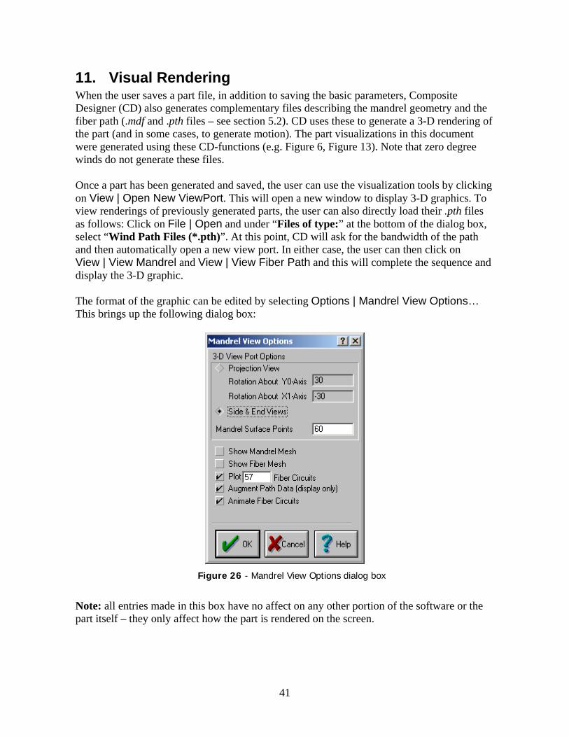
11. Visual Rendering When the user saves a part file, in addition to saving the basic parameters, Composite Designer (CD) also generates complementary files describing the mandrel geometry and the fiber path (.mdf and .pth files – see section 5.2). CD uses these to generate a 3-D rendering of the part (and in some cases, to generate motion). The part visualizations in this document were generated using these CD-functions (e.g. Figure 6, Figure 13). Note that zero degree winds do not generate these files. Once a part has been generated and saved, the user can use the visualization tools by clicking on View | Open New ViewPort. This will open a new window to display 3-D graphics. To view renderings of previously generated parts, the user can also directly load their .pth files as follows: Click on File | Open and under “Files of type:” at the bottom of the dialog box, select “Wind Path Files (*.pth)”. At this point, CD will ask for the bandwidth of the path and then automatically open a new view port. In either case, the user can then click on View | View Mandrel and View | View Fiber Path and this will complete the sequence and display the 3-D graphic. The format of the graphic can be edited by selecting Options | Mandrel View Options… This brings up the following dialog box:

Figure 26 - Mandrel View Options dialog box

Note: all entries made in this box have no affect on any other portion of the software or the part itself – they only affect how the part is rendered on the screen.

41

The top of the dialog box – “3-D View Port Options” – allows the user to select between two types of views – a diagonal 3-D projection view and a 3-face orthographic projection showing the length and both ends of the part (this tends to be useful for evaluating bottle and non-linear dome winds). Figure 27 below shows examples of both views. With the diagonal projection, the user may enter 2 angles to rotate the part in space and view it from different points. The 3-D part model is calculated by taking a 2-D part outline and revolving it. The next entry – “Mandrel Surface Points” – determines how many sample points the software should make during this revolution. The larger the number, the more circular the part cross-section becomes (e.g. a value of 4 would yield a square mandrel). Generally, the user can leave the original default of 60 unless their computer is particularly slow.

Figure 27 – shows two different projections of the same bottle. On the left are “Side & End Views” while the right is a “Projection View”. On the right, the computer is also displaying the mandrel mesh and fiber mesh, and the user is only plotting 15 fiber circuits.

The remainder of the box controls various view port settings – the first 2 checkboxes (“Show Mandrel Mesh” and “Show Fiber Mesh”) allow the user to turn on the meshes used to render the mandrel and fiber path. The next box (“Plot ___ Fiber Circuits”) allows the user to control how many passes of fiber are rendered. If left unchecked, the computer will display a default number (if the user opened the view port by loading a .pth file, then a single circuit will be displayed, otherwise it will be a complete layer). If the user checks this box, the software will plot the entered number of circuits. The fiber rendering algorithms use the fiber path points calculated during wind path generation. They then use straight lines to connect these (linear interpolation). In some cases, particularly with circumferential winds, there are significant gaps between points. This leads to coarse, blocky interpolation. Selecting “Augment Path Data (display only)” will generate many intermediate points using smooth interpolation methods. In many cases, the resulting display is more accurate. However, if the display is blocky on bottle or non-linear winds, this usually indicates too few path points – it is a better idea to use smaller dome / cylinder threshold values.

42

The “Animate Fiber Circuits” checkbox allows the user to determine if the computer should animate the rendering sequence. If unchecked, the program calculates the entire picture internally and then displays it all at once. If checked, the fiber path is drawn as it is calculated (this is not slower, so generally this box is left checked). At present, there is no provision for slowing down the rendering process. If the user wishes to use the 3-D graphic in a different software package, he/she may select View | Copy Current View. This will place a bitmap copy of the graphic on the clipboard. From there, the user may open most graphics packages (e.g. Microsoft® Paint) and utilize their paste command to import the graphic. Note: if user is editing multiple parts at once, clicking on View | Open New ViewPort generates a view port for the part which is currently being edited (i.e. the part with the active / highlighted window).

43

12. Motion Generation Once the user is satisfied with a wind path and pattern, a motion file can be generated. This is the file which will execute on the winder. For Omniwind these are .mmt or .chn files – where .chn is a chained motion file of multiple layers. For older, Compositrak systems, a .seg file is generated. There are two paths to generate motion – the user can either continue the process of entering part data, choosing a fiber path, rendering the fiber path, and then generating motion. Alternatively, the user can load and render an existing .pth file and directly generate motion from it (note that the motion generated may not be the same – see aside on page 15). If generating motion from a path file, the user must note how many circuits are required to form a complete layer – this information is not contained in the path file. Once the software is ready to calculate motion (an appropriate path has been generated) the user can simply click on Calculate | Machine Motion… to start the process. This brings up the following dialog box:

Figure 28 – The motion generation dialog box

44

One common selector box is the “Metric Units” switch near the bottom left of the screen. Check this box when using metric units. The following sections cover the entries within the box.

12.1. Machine Offsets – setting key reference locations The first heading is “Machine Offsets”. Here, the user must input the data needed for Omniwind to establish the location of the part and compensate for any tooling. This consists of two parameters: Mandrel Origin / Pattern Offset – this defines a basic mandrel parameter – the distance between the face of the mandrel or headstock chuck (or mounting flange) and the start of the mandrel part, as used for fiber path calculation. Figure 29 shows this definition. For a helical wind, the center of fiber bandwidth at the left end of the part would be located at:

Zoff + Z1

units from the zero-point of the mandrel (the chuck surface or mounting flange), where Zoff is the “Mandrel Origin/Pattern Offset” and Z1 is the “Fiber Start Position (Z1)” from the helix parameter entry window. Note that the actual, left-most fiber point would be a half-bandwidth further left (subject to the approximation described in section 6.1 under “end dwell”).

Figure 29 – definition of Mandrel Origin/Pattern Offset

45

The second parameter in this section is Payout Eye Tooling Offset. This parameter allows CD to adjust for any tooling attached to the payout system. Figure 30 shows this definition.

Figure 30 – definition of Payout Eye Tooling Offset

12.2. Motion Generation Options – selecting axis behavior The next section in the motion dialog box is Motion Generation Options. Here the user can establish which axes are enabled and set fixed positions for any disabled, but present, axes. CD supports motion in up to 6 axes, although few machines actually incorporate all axes. All machines incorporate at least 2 axes – the mandrel and the carriage. Depending on machine configuration, one or more of the fields in this box may be disabled. In the example above ( Figure 28), only 3 axes are present: mandrel, carriage, and crossfeed. The user may disable the crossfeed by clicking on the check-box next to “Enable Crossfeed Axis Motion”. In this case, actual crossfeed location is entered at “Constant Eye Position” under “Motion Generation Information” (other clearance options are disabled – see below). In a similar manner, the user may disable the remaining axes by unchecking the boxes next to “Enable Rotating Eye Motion”, “Enable Eye Yaw Motion”, and “Enable Elevation Motion”. On disabled axes, the user would enter a fixed position which that axis would assume during the wind. Under Eye Yaw, the user may select two different criteria for motion generation – either tangential to the fiber line between the payout eye and the fiber’s point of contact with the part, or normal to surface of the mandrel (aligned to a normal line connecting the mandrel’s surface and the payout eye). Fiber tangent motion is likely to generate more stable fiber control in the payout system, while normal to mandrel surface can maintain large payout systems closer to the mandrel system. The next flag in this section allow the user to reverse the mandrel’s direction. Normally, the mandrel rotates in a counter-clockwise direction when looking from the part towards the chuck. Checking “Invert Mandrel Rotation” would make the mandrel rotate clockwise.

46

Finally, the user may select “Compositrak output”. In this case, CD will generate a .seg file, suitable for conversion to a .pgm file for execution on an older Compositrak machine. Compositrak operation is not covered in this manual.

12.3. Segment Flags – for file chaining The next section of the box is titled Segment Flags. These are important during chain file generation and are normally set during chain file path and motion generation. For more information see section 15.1.

12.4. Motion Generation Information – for tooling clearance In the Motion Generation Information section, the user may alter the number of circuits to be executed and establish machine clearances during program execution. The first box allows the user to modify the number of circuits to be executed. In general, this would be modified to a multiple of the original number in order to place multiple, identical layers on top of each other. For example, if the box displays a value of 59, then entering 118 would cause the machine to place 2 layers on top of each other. Other than generating multiple layers, altering this number is not an effective way to alter fiber coverage on the part (e.g. entering 30 instead of 59 to obtain ½ coverage), because the resulting pattern would be very irregular and incomplete. To generate an even pattern which has gaps between fiber bands, the user would modify the bandwidth parameter to be larger than the actual bandwidth and execute the full program (i.e. leave the number of circuits unchanged, or perhaps enter a multiple of the number to increase the number of layers). Similarly, entering a smaller than actual bandwidth would generate significant overlaps in the final product. Unlike machining, the payout system of a filament winder should never touch the part. Therefore, the user must enter clearances indicating the distance to maintain between the fiber payout point and the surface of the part. The fiber payout point is generally defined as lying on the axis of eye rotation (for winders without eye rotation, it would lie inline with the crossfeed, perpendicular to the carriage axis) at the point at which the fiber leaves the tooling. In some simple cases, such as helical winds, clearances may be fairly tight. But often, particularly with complex parts involving multiple axes of motion, some level of clearance is very important to avoid having part of the winder or tooling strike the mandrel. At present, there are three different clearance methods available:

- Constant Mandrel Clearance – here, machine motion is scaled such that the fiber payout point is forced to lie on a curve which consists of the points closest to the part that maintain both the side and top clearance entered by the user. Side clearance is clearance in the carriage’s direction of travel. Top clearance is in the crossfeed’s direction of travel. For top clearance, the user should enter the desired clearance between the tip of the tooling / fiber payout point and the surface of the mandrel. For side clearance, the user should enter half the width of the payout tooling plus any desired clearance.

47

Figure 31 – shows how constant eye position is defined. This is primarily used for simple parts such as helixes. It effectively disables the crossfeed.

- Constant Clearance II – this case is similar to the first, except the user only enters

one value which describes a clearance distance along a normal to the surface of the mandrel. In general, Constant Mandrel Clearance (above) produces better results by allowing tighter control along both axes.

- Constant Eye Position – in this case, the crossfeed is effectively disabled (if

crossfeed is explicitly disabled as described earlier, then this is the only available option). Here, the user fixes the crossfeed at a given distance from the axis of mandrel rotation. In general, this value would be the maximum radius of the mandrel plus any additional desired clearance. This is the only option available for helix and circumferential winds. If Constant Eye Position is selected, the user can also enable Crossfeed Diameter Compensation. In this case, the crossfeed is gradually withdrawn to compensate for fiber buildup on the part. If selected, another dialog box will appear once the user clicks on “Done”, requesting information in terms of fiber build-up (i.e. crossfeed retraction) per layer.

48

Figure 32 – shows how top and side clearances are combined to establish the possible locations of the payout eye when using Constant Mandrel Clearance. Note that side clearance is defined from the center of the eye and must include at least ½ the width of the payout tooling.

12.5. Machine Velocities – establishing the rate envelope The final section of the dialog box, “Machine Velocities”, is concerned with basic motion constraints. The first selection the user makes is the type of motion rate envelope to use. The first of the three possible rate envelopes is based on having the mandrel operate at a constant speed. If this option is selected, then the user can only enter a target mandrel velocity – all other entries are grayed out. These axes will then run as fast as needed such that the mandrel can maintain a constant speed. When the program is later run using Omniwind, a feed-rate of 100% will correspond to the mandrel speed shown here. The second possible rate envelope is “Maximum Axis Speed”. Here, CD will evaluate the

CAUTIO

N: When using a constant mandrel speed rate envelope, no speed limits are enforced on the remaining axes. Caution is advised when executing a program based on constant mandrel speed – particularly with large mandrels and high target speeds. With some parts (particularly low-angle winds), execution at too high a feed rate will cause the slaved axes to lose synchronization (due to axis saturation). If the resulting position error exceeds an internal bound, the machine will execute an emergency stop. For this reason, other rate envelopes, particularly “Maximum Axis Speed”, are recommended. Other means of obtaining constant mandrel speed are described below.

49

speed of each axis during the wind and actual program execution speed at each point in time will be determined by whichever axis has the most restrictive limit.

As an example, assume a top mandrel speed of 150 rpm and a top carriage speed of 200fpm (feet per minute). If a particular portion of the wind would require the carriage to run at 250fpm to keep up with the mandrel, then all motion in that region would be slowed down to run at 80% of maximum, bringing the carriage back down to 200fpm and the mandrel to 120rpm.

One way to avoid the issue described in the caution note above and still obtain constant mandrel speed is to use “Maximum Axis Speed” as a basis for motion and to set each axis to its top speed. Then examine the resulting motion and establish the lowest speed of the rate envelope (see section 13.2 for information on viewing and editing motion and the rate envelope). This rate envelope represents a proportion of mandrel top speed.

For example, if mandrel top speed were 150rpm and a particular program had its lowest rate envelope reading at 45%, then the user would go back through the same motion generation process, again selecting “Maximum Axis Speed”, and enter a maximum speed for the mandrel of 67.5 rpm (45% of 150). The other axes would remain unchanged. The resulting motion should have a constant rate envelope indicating constant mandrel speed.

The final rate envelope is “Constant Fiber Speed”. Here the user can enter both maximum axis velocities and a target fiber speed. The software will then use approximation (based on the fiber path – which also forms the basis of part visualization) to calculate the length of fiber corresponding to each portion of machine motion. The rate at which this fiber segment is added becomes an additional, “virtual axis”. The software then begins with a wind based on constant mandrel speed. It then uses this fiber-based “virtual axis” to determine the proper machine rate envelope (i.e. mandrel speed) for each portion of the wind in order to obtain the given constant fiber speed. Finally, the software will run another check – to determine if at any time any axis is violating its speed limit. If so, the entire rate envelope is rescaled by a factor of the worst violation found. The resulting motion will obtain constant fiber speed, but depending on any final adjustment, the actual fiber speed may be less than the entered value (the actual, obtained fiber speed can be determined from the Wind Statistics dialog box, Figure 33).

As an example, assume a maximum mandrel speed of 150rpm, a maximum carriage speed of 100fpm, and a target fiber speed of 150fpm. The software would calculate an appropriate rate envelope to obtain 150fpm of fiber speed. During final evaluation, the software determines that for a particular portion of the wind, the mandrel would need to run at 200 rpm, while in a different portion, the carriage would need to run at 140fpm. No other violations are determined. The worst violation would be the carriage at 140/100 or 140% overspeed. The mandrel violation is 200/150 or 133% overspeed. Therefore, the entire rate envelope is rescaled by 100/140 or 71% resulting in an

50

average fiber speed of 107fpm. The user could determine the result from the Wind Statistics message box (see below).

Once the user has completed all entries (remembering to select Metric Units if necessary), pressing Done will bring the user to the “Motion Filter Parameters” dialog box. Here the user can enter various motion constraints to make the machine operate more smoothly (and generally faster). Motion filtering is covered in chapter 14. Once completed, a message box will inform the user that filtered motion was generated and a second box will give some basic feedback on the wind characteristics.

Figure 33 – Wind statistics feedback dialog box.

One important note on this dialog box – the data is shown at a feed rate of 50%, so if the machine were run at 100%, the fiber speed would be doubled and the wind time cut in half.

51

13. Motion Editing Once the user has generated the motion to build a part, this motion can be opened in Composite Designer (CD) for further evaluation and editing. In general, simple parts such as helixes and circumferential winds do not present many problems in terms of their motion (although smooth machine motion does not guarantee a stable fiber path – some design iterations may be needed to generate appropriate values for things like turnaround range). With more complex parts such as bottles and especially non-linear winds, the resulting motion may have some abrupt sections and these may require some additional editing before execution. At the very least, the user should open up the .mmt file to do a quick “reality check” before executing the part on a machine. This chapter covers the many means CD offers for motion editing. The most recent release of CD also includes automated motion filtering algorithms, which can greatly reduce or eliminate the need to manually edit complex motion files. Filtering is covered in the next chapter.

Caution: Filament winding is a complex process. While automated software tools often

generate files which will properly execute with little or no editing, machine operatorsare cautioned to use extreme care whenever executing a particular program for the first time. Programmers and operators should also visually inspect each program’s trajectory before it is run to make sure there are no obvious problems. This is even more critical whenever running manually edited motion files since clearances may have inadvertently been reduced and/or entire segments of motion added.

13.1. Overview of motion generation process Before getting into the details of editing motion, a brief word on how motion is constructed in CD. This is to assist the reader with understanding some of the intricacies of motion editing. CD uses two separate processes for generating motion – for some special cases such as helical winds and circumferential winds, motion is directly generated to match the parameters entered during part creation. For example, the carriage axis motion on a helix is as follows:

- The carriage begins at one end of the part - It accelerates at the appropriate rate to reach the fixed speed required to generate the

desired angle at a particular mandrel speed – this acceleration rate is set by the required speed and the turnaround range

- It then coasts at this fixed speed to the end of the constant fiber angle section - It decelerates back to a stop over the given turnaround range - It dwells for the necessary amount of time / mandrel degrees - Finally, it repeats the steps above while heading in the opposite direction

This would complete one circuit.

52

The second approach is to begin with the fiber path and use various mathematic transformations to establish the correct location of the various machine axes corresponding to each point in the fiber path. Then the software connects these machine coordinates to generate a complete motion trajectory. All bottles, non-linear winds, and path based chain winds are generated in this manner. As was mentioned before – all motion is tied to the mandrel, which represents a “master timekeeper”. The mandrel operates at a constant rate and all other machine axis coordinates are calculated to correspond to given positions of the mandrel axis. This becomes apparent when editing the motion file – the mandrel axis is generally a straight line which starts at 0 degrees and ends at however many degrees are required for one complete motion circuit. Note that it is possible to edit and alter the mandrel’s motion. In order to do this, the software uses an additional axis called the “Virtual Mandrel” or VM. Before editing, the VM directly corresponds to the mandrel motion. In the various motion editing screens, the horizontal (x) axis corresponds to the VM while the vertical axis (y) corresponds to the axis being edited. If the mandrel axis is altered, it no longer corresponds directly to the VM, but is mapped to it, just like the other axes. In effect, the VM axis corresponds to time – with one modification: the rate envelope. The rate envelope is used to globally scale the machine’s velocity across all axes. This rate envelope was introduced in order to enforce various limits on machine motion (for example when generating constant fiber speed or maximum axis speed programs).

For example, if a machine has a top mandrel speed of 150rpm, the rate envelope is a flat 100%, and the mandrel has not yet been edited (i.e. it simply corresponds to the VM), then the mandrel will run at a constant 150rpm – and the other axes will track the mandrel as needed. If the rate envelope drops to 50% at some point in the circuit, then all axes would effectively run at 50% during that section - the mandrel would drop to 75rpm.

Finally, when running the program on Omniwind, all motion is once again scaled by the operator through use of the increase and decrease buttons (see section 17.4).

13.2. Motion Editing, first steps To begin the editing process, the user first opens the motion file in question – File | Open (note that motion files are the default files on display). Figure 34 shows a typical screen – the carriage motion of a particular file. The screen has 3 sections which share a common x-axis representing the virtual mandrel (VM) location. The y-axis varies by section – for the top region it displays plots axis location, the mid-region displays velocity, and the bottom region displays acceleration. A small window also appears which displays the value at the current pointer location. Note that velocity and acceleration are calculated against the VM (e.g. velocity units are inches or mm per radian of VM motion). In general, the magnitude of

53

velocity and acceleration is of limited value – the screen is meant to be a graphical representation and allows the user to quickly evaluate potential problem regions. Probably the first command of interest is the use of the Edit Axis Motion menu header. From this header, the user can select which axis to display. Up to 6 axes plus the rate envelope are available (depending on machine configuration). Each axis uses the same basic format as the figure below except for the rate envelope, which does not have velocity or acceleration vectors. Displaying the rate envelope will also quickly calculate and display the current wind time of the program at a 50% machine rate. One point to note – the screens are automatically scaled so that each chart line uses up its portion of the graph. This scaling takes place each time the user switches axes and also when data points are edited. Clicking on Edit Axis Motion | Enable Auto Scale will cause any screen update to automatically rescale for the displayed data. The remaining commands under this heading will be covered later.

Figure 34 – shows a typical motion editing window (note that the graphics have been inverted for better printing – original colors are green lines on a black background). This graph shows the carriage motion which for bottle similar to Figure 27 (with a lower wind angle).

At this point, various tools exist to assist the user with editing the given file – many of these are accessible through the toolbar at the top of the screen or by using the right mouse button. Once the user has quickly scanned each axis, a typical procedure would be to check for any

54

acceleration spikes. Figure 34 shows 2 clear acceleration spikes. These would be candidates for removal. Generally, the first step is to zoom in on the problem region. To do this, the user clicks on the zoom toolbar button: This will add a small magnifying glass to the cursor. The next step is to drag a box around a region of the graph for closer inspection (press and hold the left button in one corner of the region, then drag the mouse to move the pointer to the opposite corner of the region). As soon as the left button is let go, CD will zoom in on the target region. Note: to zoom in more than once requires multiple clicks on the zoom toolbar button – the default mode of the cursor is to select points. To select a point or points, the user once again drags a box around the region to be selected. If the user is not happy with the selected groups, he/she can hold down the left Shift key and press the right mouse button to release the selected points and try again. The left-shift, right mouse button combination will cancel out of any current editing mode.

Figure 35 – shows the various steps used to reduce an acceleration spike. Top left shows original motion with 2 high-acceleration regions and a box around zoom region. Top right shows zoomed region with box around points to be smoothed. Bottom left shows original with smooth motion overlaid (green line). Note about 50% reduction in acceleration peak. Bottom right shows selection of point at peak acceleration – to be deleted. Note use of crosshair to assist with selection of point.

55

Quite a few means are available for tweaking motion in a particular region. One easy method is to use the built-in smooth function. To do this, the user selects a group of points around the region of interest (roughly symmetrical around the peak acceleration point). For smoothing to work, it requires a minimum number of points – the actual number depends on the setting of the Bézier Smoothing Factor (see page 62) and varies between 9 and 20 (low factors generally require fewer points). Once a region is selected, the user right-clicks, then selects Edit Range | Smooth Range. A smoothing function is then applied to the given points. Whenever motion is edited, the new data appears as a purple, superimposed graph (note the colors are reversed in the screen-shots for this manual). If the new data appears acceptable, clicking on the accept new dataset toolbar button will finalize the change. Alternatively, the discard new dataset button will revert to the previous data.

Caution: In general, editing and smoothing (and later filtering) can work quite well to improve machine motion, although some caution is in order whenever trajectory points are modified. The user should understand what the motion graphs represent and the implications of any position changes – in particular, how changes to the crossfeed and carriage affect machine to part clearances.

For bottle-like parts, typical motion consists of the carriage moving back and forth across the length of the part and decelerating at the ends where the crossfeed plunges in. In such a case, increasing large position values and decreasing small ones will increase part clearance because the carriage have more overshoot at the ends of part.

Similarly, for the crossfeed, typical bottle motion is a constant position over the length of the part and plunging in at the ends. In this case, all reductions in crossfeed’s position value will bring the crossfeed closer to the mandrel.

In many cases, smoothing rounds off corners which tends to reduce clearances, so the user is advised to evaluate the amount of position change when performing any edit. One reasonable idea is to give the machine more clearance than is necessary during motion generation. Once motion is smooth and there is still excessive clearance, then entire axes can be rescaled to reduce clearances at the ends (see page 60).

While these guidelines apply to bottle-like parts, they cannot be generalized to arbitrary, non-linear winds. The user should try to picture how the motion graphs translate to motion on the machine and whether a particular edit will increase or decrease clearance.

While smoothing was able to reduce the acceleration spike, in some cases, the simplest method is to simply delete one or more key points. The best way to accomplish this is to zoom in quite closely on the set of points near the acceleration peak. Next, turn on the cursor

56

crosshair (to do this, right click on the mouse and select “Toggle Crosshair”) – this tends to assist in selecting the correct point. In this way, the user can align a particular coordinate (denoted by small “x” in the position window) with the acceleration spike. Once this point has been selected, pressing the delete key or clicking on the delete button will remove the point and show the resulting data. In the example (Figure 35), removing the data point at the acceleration spike, together with smoothing, reduced the acceleration spike by about 75% without introducing significant errors (Figure 36).

Figure 36 – shows motion after the edits from the previous graph are completed. Note that the left (edited) acceleration spike is now much smaller than the right one – peak values have been reduced by about 75%.

An even simpler method to smooth out spikes is to select the entire trajectory (right click and select Edit Mode Options | Select All). Now perform smoothing operations again. Generally the resulting data shows a marked reduction in acceleration values (but again, caution is advised due to clearance issues). For this example, executing a smoothing operation on the complete axis reduced acceleration spikes by over 90% but introduced some significant position errors (Figure 37). These are probably the most common editing steps for smoothing motion. One important note is that smoothing the rate envelope is just as important as editing any particular axis since it causes accelerations on all axes. Unfortunately, in many cases the rate envelope is

57

rather noisy. It can be smoothed in similar manner, but some caution is in order. In general, reducing the rate envelope at any one point doesn’t present any issues, but increasing it may cause one or more axes to exceed their rated limit if the machine executes the part at 100%. One approach is to smooth the entire envelope and try the resulting motion at a low machine feed rate - gradually increasing the speed and checking if any axis appears to approaching its limit (this can be done by examining Omniwind’s screen).

Figure 37 – shows effect of selecting entire curve and applying filtering. Note the lack of spikes on the green acceleration line – values were reduced by over 90%.

13.3. Additional Viewing and Editing Commands Beyond simple point deletion and smoothing, there are quite a few tools available for motion editing. Most of these are accessible via the pop-up menu (clicking the right mouse button), via the toolbar, and via the main menu. Before much motion editing can take place, a range of motion coordinates needs to be selected. This was briefly covered in the previous section. The basic concept is common to most Windows graphics software – the user clicks and holds the left mouse button while dragging a box around the points to be selected. Note that selection only works in the position portion of the window (the top graph).

58

To select the entire graph (or an entire segment of a multi-segment chain file), use the Edit Mode Options | Select All pop-up menu item. This will select all points visible on the screen (the entire program for a single segment, non-zoomed display). On multi-segment files, all visible points of the segment with the greatest proportion displayed on the screen will be the one selected – to select all points of a particular segment, use the zoom functions covered below and ensure that the entire segment to be selected is displayed. Range selection is the default behavior for the mouse pointer while editing the motion file (other behavior is indicated by a different pointer). To cancel a selection (or the current mouse pointer mode), hold the left shift key and press the right mouse button. Finally, after any editing is complete, the screen displays the original, green motion graphs together with purple lines representing new motion. At this point, the user can accept the changes by one of the following: selecting the menu item Calculate | Accept New Dataset, via the toolbar button, or via the Edit Mode Options | Accept Results? pop-up menu item. Similarly, to reject the edit and revert to the original dataset, select Calculate | Discard New Dataset, press the toolbar button, or select the Edit Mode Options | Discard Results? pop-up menu item. In both cases, a pop-up window appears to verify the selection. Another important editing function is to get the display to show the relevant region of a given trajectory. While some commands edit the entire trajectory, often the user is only concerned with editing a particular range. To assist with this, there are various zoom commands which are accessible via the toolbar and via the View | Zoom Menu submenu. The zoom function – or Zoom Window command – places the cursor into zoom mode where the user can drag a rectangle across a range of points to indicate the region to zoom into. Note: after zooming, the cursor reverts to point selection mode; multiple zooms require multiple clicks on the zoom window button. Zoom Previous or will revert to the previous zoom window, i.e. if the user zooms into a region, then zooms again and decides the second zoom was too much, this command will revert to the first zoomed region (rather than forcing the user to revert to the full dataset and start over). Zoom All or will show the complete data set again (no zoom). Scroll Left or will shift the window to the left (earlier in time) by 10% of the window at its current zoom level. Scroll Right or will shift the window to the right by 10%. Often, during machine testing of a wind pattern, it becomes necessary to do some minor tweaking. For example, the clearance might be slightly inadequate – particularly once several layers of fiber have been laid down. The Transform Dataset menu heading on the pop-up menu contains various tools to adjust an entire axis (Figure 38 shows examples of these commands):

- The axis can be mirrored – this results in mirroring the data horizontally (inverting the time axis). Mirroring is useful for certain types of unusual fiber payout configurations, although in many cases, the same results can be obtained through some combination of inverting the mandrel rotation, inverting the eye rotation, and/or

59

starting the layer on the right side of the mandrel. Be very cautious when mirroring – especially on the crossfeed and carriage – they generally need to be mirrored together.

- The axis can be offset – which moves all axis positions in a particular direction. Clicking this menu item generates another dialog box allowing the user to enter the offset for the axis being edited. Offsetting is useful if the motion is essentially correct but the mandrel location is slightly different than was first entered. For example the tooling might have changed or the start of the mandrel might vary for some reason. In cases where significant editing has already taken place, it is usually faster to add an offset to the necessary axes rather than generating motion again with different clearances. Offsetting the machine can also be performed in Omniwind – but by using the Offset Dataset menu item, the change can be made permanent. Offsetting follows the conventional axis definitions used throughout CD and Omniwind (e.g. positive value for carriage offset would cause the program to move closer to the tailstock).

- The axis can be rescaled – which allows the user to set different end points for the axis and the resulting motion will be linearly interpolated to lie between the new end points. This allows the user to rescale, offset, and vertically mirror (by reversing maximum and minimum values) the data in one step. This is often handy when trying to tweak clearances or, in some cases, “fool” CD. Vertical mirroring can invert motion on most axes (do not use on the crossfeed – and as usual with such major edits, use caution and ensure consistency between axes. Use of other inverting options during path and motion generation is recommended instead). For example, if the user is trying to obtain a particularly low wind angle on a bottle but the mandrel has a large shaft – this would prevent the user from entering a small polar opening. In some cases, it may be possible to work around this problem by generating motion assuming the small polar opening. If this motion were run, the crossfeed would strike the mandrel, but rescaling the crossfeed’s motion – by leaving its maximum value unchanged and increasing its minimum value – can generate sufficient clearance. In many cases, the resulting path is unlikely to be stable, although pin-rings, or in some cases the mandrel shaft, can help prevent excessive slippage.

- The axis can be converted to a second order polynomial (or “functional” motion – i.e. each region of motion has a fixed acceleration rate). This command will attempt to determine a reasonable second order approximation to any given trajectory; however it is usually of limited value. For zero-degree, circumferential, and helical winds, CD normally uses functional motion, but for various reasons, this might have been changed to cubic or linear interpolation. If the user wishes to restore functional motion to a particular wind, this should be done directly via the motion table and not through the use of this command (see section 13.5).

60

Figure 38 – Examples of the Transform Dataset commands on the carriage axis for a bottle wind: original motion in purple, new in green. Upper left: mirroring the axis – note the alteration is horizontal (time-based) not vertical (position-based), in some cases these produce the same result but generally they don’t. Upper right: Offsetting the axis – for this carriage axis view, all motion has been moved towards the tailstock (up on the screen). Bottom: rescaling the axis – new motion is inside of old motion – the carriage won’t travel as far on either extreme.

The Edit Range pop-up submenu includes various functions for editing a range (a selection) of points (Figure 39 shows examples of these commands). Remember that selecting a range is as simple as dragging a box around the points. The individual commands:

- The points can be deleted (also accessible via the delete key, the toolbar button, or the Calculate | Delete Range command on the main menu). This simply deletes the points, maintaining whichever interpolation was in use for the axis. It is often useful for reducing a high-acceleration point or small region.

- The range can be smoothed (see section 13.2 above more a more detailed description of this)

- The range can be interpolated – via linear or cubic interpolation. In both cases, the software will replace the points between the start and end points with a new number of points defined under Edit Range | Set Parameters (see below). With cubic

61

interpolation, the new points follow the original contour (useful for reducing the number of points) while with linear interpolation, they form a straight line between the first and last selected points.

Figure 39 – Examples of various Edit Range commands – note: the purple line is before and the green is after the edit. Top left: deleting the range (note how cubic interpolation between remaining points smoothes motion); top right: smoothing the range produces tighter motion but still reduces acceleration, bottom left: cubic interpolation follows the contour even tighter but can still generate some smoothing by reducing the number of points; bottom right: linear interpolation produces an abrupt change in velocity to generate a line connecting the endpoints.

The final option on the Edit Range submenu is Set Parameters. This command brings up a dialog box allowing the user to edit various parameters for other functions on the submenu. The topmost parameter, Bézier smoothing factor, affects the smoothing algorithm. This algorithm requires various internal parameters and this number selects one of nine different parameter sets. In general, larger numbers generate a greater smoothing effect and use a larger dataset when averaging. The rest of the box deals with linear and cubic interpolation. The use of Thresholding is not recommended. With Uniform Calculation Intervals, the user selects how many evenly time-spaced points the interpolation functions should generate – note: this many points will be generated for the entire selected range regardless of its size – this can be useful for

62

generating more or less data points on any given dataset. The final selection establishes the end-point criteria for the spline curves. Generally Parabolic is used except when editing an entire trajectory at once, then Circuit is used.

13.4. Direct Motion Generation So far this chapter has focused on various tools available to view and alter the existing motion profile. It is also possible to directly edit the data, either by drawing points with the mouse, or by editing the motion tables (see following section). Here we will deal with using the mouse to draw data. There are two options for this – one is the Draw Data Directly command on the pop-up menu, the other is via Calculate | Insert Points (equivalent to the

toolbar button). Before starting, the user should select an appropriate zoom level to ensure that the newly entered points will not introduce significant position error. Draw Data Directly is probably the easier and more powerful point entry tool. When selected, the user is first warned of the danger of direct data entry. At this point the mouse changes to a pencil and the user can simply add points by positioning the mouse and clicking the button. The resulting motion will erase any existing points in the same region as those entered. Caution: On multi-segment parts, use care at segment boundaries – the current function does not enforce boundary conditions (if a particular segment is periodic – i.e. it has more than one circuit – then all axes except the mandrel must begin and end at the same location). The Insert Points command is similar, except that existing data points are not removed – old and new points are both combined to form the new motion – in many cases resulting in wild oscillations. Generally, the user would manually delete any offending points later. This mode is handy where the user specifically wants to add points. It does not pose any issue at segment boundaries since it doesn’t delete any points.

13.5. Motion Table Editing An alternate method to edit motion is via the motion table. This gives the user very precise access to the motion of all axes at once. Note: only one form of entry is available at a time – if the motion table is open, the user is unable to do any editing of the graphs. To display the motion table, click on Edit Axis Motion | Motion Table. The table is arranged as a spreadsheet with 10 columns, which are covered in the following text. Segment Info: this contains basic information about each segment (on chain files, each segment, including transitions, will have an entry in this column). This column has the following format: Seg. #X, "NAME", Circuits=Y / Strokes=Y where X is a sequential segment number (note: this is not user adjustable – even if altered, CD will auto-number the segments when the table is closed). NAME is the segment’s name, up to 20 characters. NAME is used at various locations including the operator’s display when running the part. “Circuits” or “Strokes” indicates how to interpret the number Y, which is a number indicating how many times to execute the segment. It is important in determining if a

63

segment requires alignment of its start and end points (i.e. whether all axes, except the mandrel, must return to their starting locations to begin the next circuit). Most types of winds generate Circuits. If Y is one then the circuit only executes once so start and end points no longer need to align. Strokes are slightly more complex – they are only used for circumferential winds and count a single motion of the carriage either towards the headstock or the tailstock. If Y is one, the segment executes once leaving the machine at a different position. If Y is an even number, the entire segment executes Y/2 times. If Y is 2 then start and end points need not align, otherwise they must. If Y is odd and greater than 2 then operation depends on whether or not the program is in a chain file. For single segments, operation will stop ½-way through the final pass, otherwise the program will automatically generate 2 chained circumferential windings, the first having an even number of strokes and the second having a single stroke. This permits proper alignment between segments. Note: at all segment boundaries, the end point of the first segment is the starting point of the second segment. Also, at these critical points, all remaining columns must contain data for all defined axes. Flags: these define machine behavior in this segment and also establish which type of interpolation to use for each axis. Following format is used: [SegFlag…], Mandrel=IF, Carriage=IF, [Elevation=IF], [Crossfeed=IF], [Eye Yaw=IF], [Eye Rotation=IF] where [] indicates optional entries, SegFlag… indicates one or more of the possible segment flags. These are:

- OffMand – mandrel offset, allow the mandrel to continue from segment to segment without returning to zero location.

- Hold – automatically hold the machine at the segment boundary. - AutoFP – only for use on transition segments – this will automatically stop the

machine, perform a Find Path for the next segment, and start up again (depending on whether the Hold flag is also set). The transition segment is essentially ignored.

Generally, for a multi-segment file with smooth transitions, only OffMand would be set for each segment (but not necessarily the first segment). Note that these flags can also be set via a more user-friendly method when creating the chain file (see section 15.1). The remaining column entries are interpolation for each existing axis. The axis names are exactly as they are shown above, while IF is one of the following interpolation flag options:

- Cubic – uses cubic spline interpolation, generally the most common format for motion of any complexity.

- Functional – uses functional, second order, constant acceleration interpolation. This is the most common format for simple motion files (helixes, circumferential, and zero-degree winds) which are already based on functional motion. It will not produce reasonable motion for complex, path-based motion.

64

- RFunctional – relative functional – also uses second order, but relative rather than

absolute position information. This segment is not periodic and continues relative to its starting position. Very rarely used (never automatically generated).

- Linear – use linear, constant velocity, interpolation. This is generally only of use for files with a very large number of points such that velocity changes between sample points are minimal, otherwise the machine will experience very large accelerations.

For the most part, the user is unlikely to change any interpolation flags. In some cases, motion which had functional interpolation might have accidentally been switched to cubic. This column allows the user to restore the original setting (and use different settings in different segments). Indp. (ds) contains relative time entries expressed in seconds. Relative (or incremental) time is used to ease insertion of new data. Actual program execution time is established via this column, modified by a linearly interpolated rate envelope, see below, and further affected by the execution rate set by the machine operator control. This column is somewhat difficult to directly edit. It is often easier to use graphical functions to insert new motion points on the axis of interest and the use the table to enter exact positions for those points. However, if the user needs to add fiber length at a particular location (i.e. additional mandrel rotation), then this usually requires new entries (or similar calculations) to be made in this column. For more on altering this column / inserting additional mandrel rotation, see section 13.7. Note that unlike the axis columns, each row of the time column requires an entry – this is fairly intuitive, since the software needs to know the time for each machine coordinate. Also, this column is used by the software to determine the end of the program – which is the first blank entry. The next columns (Mandrel (dø), Carriage, Crossfeed, Eye Rot., Eye Yaw, and Elevation) indicate the machine coordinates at any given time point. The mandrel, similar to time, uses relative (or incremental) coordinates to make editing and inserting new points easier. The remaining axes use absolute coordinates since their motion is bounded and cyclical. The units are degrees for rotary axes and either inches or millimeters for linear axes (to switch systems, select Edit Mode Options | Display Metric Units from the pop-up menu on the motion graphs). The user can navigate through the spreadsheet, searching for a particular region of the wind, and then directly modify the contents of these columns. As with all motion editing, caution is advised. Also, while the mandrel can also be directly edited, this process is more complex than for the other axes. Changing mandrel entries directly affects the fiber length of the part and can have a significant affect on the pattern and fiber stability. This issue is covered further in section 13.7. Individual position cells can be left empty. Only the first row in each segment and the final row of the entire program requires entries for each present axis (as well as the rate envelope). The software will automatically apply the given interpolation method to generate intermediate points where these are left empty.

65

The final column is the Rate Envelope. The rate envelope scales the time (Indp. (ds)) column. For example, if the rate envelope is at 20% and a time-column entry is 0.4, then the motion from the previous row to the given row would take 2 seconds (if the machine is running at 100%). The rate envelope itself is linearly interpolated from one entry to the next – gradually accelerating or decelerating all axes along the way.

13.6. Spreadsheet Table Functionality The motion table window is actually a type of stripped-down spreadsheet and offers many spreadsheet-like editing functions. In addition, whenever the table is open, several additional menu functions become available. This section covers these features. For the most part, editing features are fairly similar to most Windows spreadsheets: To move around the file, use standard mouse or keyboard control. Click on a cell or using the keyboard to move to the cell selects that cell. To replace the contents of the cell, simply start typing. Pressing the Enter key accepts the current edit, while the Esc key discards it (use caution with the Esc key – if no cell is selected, it will discard all edits and return to the graphical motion window!). Note: when closing the table window, the user is given an additional opportunity to accept or reject all changes. To edit (without replacing) the contents of a cell, double-click on it. At this point, common Windows keyboard editing commands can be used (e.g. Ctrl-C to copy a block). To quickly move around the file with the keyboard, the user can use the Control and arrow keys – these will either skip over neighboring empty cells to the next occupied cell, or skip over neighboring occupied cells to the last one. For example, positioning the cursor in the first row and column and pressing Control + Down Arrow will place the cursor in the first row of the second segment (also, Control + Page Up / Down will move the screen over to the left and right, but this is of limited use since the sheet only has 10 columns). To replace the contents of a cell, select the cell with the mouse or cursor, To delete a cell, select the cell with the mouse and press the delete key and select “All” in the dialog box which appears (generally, this can be done quickly by just pressing the Enter key). Multiple cells can be deleted in the same way. There are various options for selecting multiple cells – the user can drag the mouse to form a box, hold the Control key down and press the left mouse button in each cell, or hold the Shift key down and use the cursor keys (or the mouse) to select a rectangular block. Finally, the user can click on a particular row or column heading to select the entire row/column, or in the top left corner square to select the entire spreadsheet. Moving, copying, and repeating cells is also accomplished with the mouse. To move a cell or group of cells, first use the mouse or keyboard to define a block (only a single block may be used, not multiple selections via holding down the Control key). Now place the mouse at the boundary of a selected block – the pointer should change from a “+” to a typical arrow-pointer. At this point, hold down the left button and move the mouse the desired number of

66

cells – the outline of the selected block will move to the new location. Finally, when the button is released the cells are moved. Any newly exposed cells are cleared. To copy the cells, the procedure is the same, except the user should also hold the Control key during the move operation (note that copying does not work well if the new location overlaps the original location). Finally, to repeat the cell, first select the cell(s) to be repeated. Next, move the mouse pointer over the small “+” in the lower right corner of the block (the pointer also changes to a small “+”) and drag the block in the direction to be repeated - either vertically or horizontally, but not both in a single operation. If the block contains formulas, these are transposed as described next. The spreadsheet also supports common formula evaluations. Formulas can be used in any cell – when the data is converted back into motion format, the formulas are evaluated. In addition, any cells beyond the first empty time (Ind. (ds)) entry can be used as a “scratchpad” (keep in mind that formulas are lost when closing the table view, see exporting and importing below). The spreadsheet follows typical spreadsheet conventions:

- an equals sign begins a formula - column letters and row numbers indicate cells - functions and standard computer math notation are used calculate values - colon notation indicates a range of cells - e.g. sum(a1:b4) would sum the 8 cells from

column 1 row 1 to column 2 row 4 As an example, if a cell contained the following formula:

=C20*4+SQRT(D4)/2 and the cell at column 3 in row 20 (or C20) contained 5, and the cell at column 4 row 4 (D4) contained 16, then this cell would evaluate to:

=5*4+SQRT(16)/2 and display 22 after the user pressed Enter. When cells are copied or repeated (but not when moved), they are transposed. This means that their cell references are modified by the number of cells moved. For example, if the formula above were copied one column to the right and one row down it would become:

=D21*4+SQRT(E5)/2 This is useful when doing calculations on blocks of values. To prevent transposition, place a dollar sign in front of the column and/or row which should remain fixed (e.g. $C4 would have a fixed column and transposable row). The following is a list of all available spreadsheet formula functions:

67

List of Spreadsheet Commands ABS ACOS ACOSH ADDRESS AND ASIN ASINH ATAN ATAN2 ATANH AVERAGE CALL CEILING CHAR CHOOSE CLEAN CODE COLUMN COLUMNS COS COSH COUNT COUNTA DATEVALUE DAY DB DDB DOLLAR ERROR.TYPE EVEN EXACT EXP FACT FALSE FIND FIXED FLOOR FV HLOOKUP HOUR IF INDEX INDIRECT INT IPMT IRR ISBLANK ISERR ISERROR ISLOGICAL ISNA ISNONTEXT ISNUMBER ISREF ISTEXT LEFT LEN LN LOG LOG10 LOOKUP LOWER MATCH MAX MID MIN MINUTE MIRR MOD MONTH N NA NOT NOW NPER NPV ODD OFFSET OR PI PMT PPMT PRODUCT PROPER PV RAND RATE REPLACE REPT RIGHT ROUND ROW ROWS SEARCH SECOND SIGN SIN SINH SLN SQRT STDEV STDEVP SUBSTITUTE SUM SUMSQ SYD T TAN TANH TEXT TIME TIMEVALUE TODAY TRIM TRUE TRUNC TYPE UPPER VALUE VAR VARP VDB VLOOKUP WEEKDAY YEAR This section is only intended as a brief overview of spreadsheet functionality. These features are primarily incorporated to allow quick, simple motion editing and basic formula entry. Note: keep in mind that the various CD file formats are all value based – any spreadsheet formulas will be lost when the file is saved. To allow the user to track formulas and also provide an interface to a far more powerful spreadsheet, tables can be exported and imported in Excel® 4.0 format. This is accomplished via the Axis Motion Table menu header and the items Import Excel 4 File and Export as Excel 4 File. Once the file is in Excel format, the user can make use of the wide assortment of features available in Excel. Keep in mind that the file must also be saved in version 4.0 format so that CD can import it again. Two additional, advanced editing functions are covered in the following sections – directly inserting motion into the table, and merging separate motion files. Once all modifications are complete, closing the table window will ask the user if they wish to apply the changes. Afterwards, checking the resulting motion graphs and further graphical editing can help to smoothly transition to any altered motion.

13.7. Inserting motion via the table This section describes how to modify a motion table file to add fiber length. Note that doing this will significantly alter program behavior, but it can be quite useful to generate specific

68

winds. Examples include hoops or other recurring patterns within a more complex wind such as a bottle, or local fiber build-ups at fixed carriage locations. These are often difficult or tedious to automatically generate and properly chain. Editing the motion file should always be done with care. It should generally be the last step in a programming process because if motion needs to be regenerated later, all editing is usually lost and needs to be repeated. Finally, if the resulting file (or segment) is still expected to form a closed pattern, then any inserted mandrel length needs to be chosen with care. Ensuring a particular pattern with pattern closure requires some detailed analysis of the mandrel’s motion (see appendix 19), but one simple case always maintains the original pattern: adding any number of complete hoops (360 degrees). Before starting to edit the program, it is helpful to have plenty of entries in the mandrel column. If the file was generated via motion filtering, then this is already the case. Otherwise, the user can generate mandrel entries by using linear interpolation on the mandrel axis (see page 61). Ideally, the table will have sequential mandrel entries on both sides of the insertion point (Figure 40).

Figure 40 – a motion table which is well suited for inserting additional mandrel rotation

The first step is calculating the mandrel’s speed (in degrees per second). To do this, divide the change in mandrel angle (entries in the Mandrel (dø) column) by the change in time (the Indp. (ds) column). Note – these are both incremental measures. For example, if the mandrel has no entry in the previous 3 rows, the user would need to the sum the Independent entries in these rows plus the row containing mandrel data and divide by this value (the spreadsheet functions described above can assist with this step). With this information, the user can now insert some motion. It is often easiest to insert a few rows (as described above, page 66), although existing entries can also be altered to achieve the same effect. When inserting rows, simply enter mandrel values which sum to the desired additional rotation (e.g. 4 entries of 360 would add 4 hoops). In the Indp. (ds) column, enter the duration of each motion – generally keeping with the current speed, although gradual accelerations or decelerations are also possible. Using the example figure, the mandrel is rotating 44.9 degrees every 0.0648 seconds or 692.5 degrees/sec. So if the user wished to enter 4 new rows of 360 degrees each, the independent time column would contain 0.5199 seconds for each mandrel entry. This would maintain the same constant speed. If altering

69

existing segments, the user should add any changes to the current entries in those segments – e.g. the mandrel entries in the figure would change from 44.9 degrees to 404.9 degrees and the time entries from 0.0648 to 0.5847. Finally, once the mandrel motion has been inserted, all editing functions can be used to further refine, insert, smooth, and otherwise alter the remaining (and even the mandrel) axis to obtain the desired result. As is always the case, the machine operator should be very cautious when executing any program for the first time, particularly edited ones.

13.8. Merging Motion Files and Manual Chaining If the user needs more direct control to chain separate files together, they can directly insert entire segments into the motion table and manually join these. Note that the user is also responsible for setting appropriate transition flags and ensuring that motion transitions are sufficiently smooth. Some examples might include inserting a single-pass fraction of a particular wind to move the machine into a specified location before commencing with another segment, or a means to mix and match winds generated via different methods (At present, the chain wind module doesn’t support mixing path and motion based transitions – meaning zero degree winds cannot be chained by path). Obviously, the normal caveats apply – always use extreme caution and very slow machine execution rates when running any manually edited files for the first time. Also, review the resulting motion graphically to do a quick sanity check. We now assume the user wants to insert a particular motion file at a given location. If that location is the end of the file, they can simply insert the new file – otherwise they first need to ensure that there is sufficient room for insertion (existing entries are not automatically moved – they are overwritten). To see how many rows are required, they could open up that motion file and inspect its motion table. Moving part of the spreadsheet is covered above (see page 66). To break up the existing file, the user should select the block beginning with the first row after the segment boundary entry (i.e. after a row which has data in the Segment Info column – unless the user wants to insert at the start of the file before initial motion: then move the entire program down). From there to the end of the file, all rows need to be moved down a sufficient amount (usually a little more than the number of entries to be inserted). If the new file already matches the existing file (for example, it might be a copy of an already existing segment), then it can be inserted directly at the end of the previous segment. Otherwise the user should probably consider including a few additional rows for transition motion. Once the insertion location is clear, the user would position the cursor in the first column (“Segment Info”) of the appropriate row and select the menu item Axis Motion Table | Insert Motion File. The new file should now appear at the given location. If transition motion is required, the previous section gives some basic pointers for generating it. The user would typically insert a considerable length of fiber (i.e. mandrel rotations) while

70

manually inserting reasonably smooth transitions on the other axes from the end point of one segment to the start of the next – gradually adjusting carriage and eye-rotation speed to form a (hopefully) stable transition (note this motion can later be tweaked and smoothed using the graphical interface). Keep in mind that unless both the position and velocity match at segment boundaries, the machine is going to try to “jump” from one state to the next. Also, for cyclic segments (any segment with a stroke count > 2 or a circuit count >1), segment start and end points must match. To avoid this, the user will usually need to copy a particular segment and alter its circuit count to 1 so that it can become non-cyclic. Finally, when generating transitions consider mandrel shape and the potential for striking the surface, particularly the machine location defined by carriage and crossfeed values. Once the transition is done, the user may proceed with combining the endpoint of the previous segment with the new motion (or if motion was inserted at the very start of the program, the same process takes place at the end of the inserted block). Figure 41 shows what a segment boundary between the existing end of file and a freshly inserted segment (motion file) might look like. Note how all axes except the mandrel (and time/independent) are aligned. This is as it should be. To complete the transition, lines 41 and 42 must be combined – remember that the last line of a segment is also the first line of the next segment. If the new file was inserted between existing segments, then line 41 would also have Segment Info and Flags entries. These would first be moved into the last row of the freshly inserted segment(s). Next, the Segment Info and Flags entries from row 42 must be moved to row 41.

Figure 41 – shows a motion table with a freshly inserted file at line 42, the previous end of file. This requires manual editing to tie the end and start points together.

The remaining axes on row 41 are now valid – they are either the same as their counterparts on 42, or they are incremental values (for time and mandrel) which are not used on the first line of a program. Now row 42 can be removed by moving all remaining rows in the program up by one (starting with row 43). Important: except for the very first line in a program, no time (Indp. (ds)) column entry should be zero! This will generate an error. Finally, if there are additional segments after the inserted motion, the process is repeated at the end of the inserted segment. This would complete appending a matched motion file to the end of an existing file. Figure 42 shows the result after the insertion is completed. The user does not need to worry about updating the segment number, but should consider setting appropriate segment and interpolation flags.

71

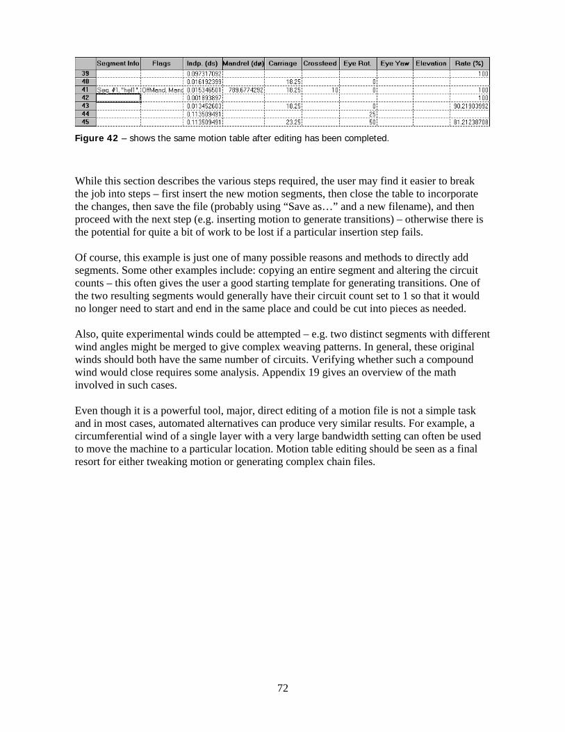
Figure 42 – shows the same motion table after editing has been completed.

While this section describes the various steps required, the user may find it easier to break the job into steps – first insert the new motion segments, then close the table to incorporate the changes, then save the file (probably using “Save as…” and a new filename), and then proceed with the next step (e.g. inserting motion to generate transitions) – otherwise there is the potential for quite a bit of work to be lost if a particular insertion step fails. Of course, this example is just one of many possible reasons and methods to directly add segments. Some other examples include: copying an entire segment and altering the circuit counts – this often gives the user a good starting template for generating transitions. One of the two resulting segments would generally have their circuit count set to 1 so that it would no longer need to start and end in the same place and could be cut into pieces as needed. Also, quite experimental winds could be attempted – e.g. two distinct segments with different wind angles might be merged to give complex weaving patterns. In general, these original winds should both have the same number of circuits. Verifying whether such a compound wind would close requires some analysis. Appendix 19 gives an overview of the math involved in such cases. Even though it is a powerful tool, major, direct editing of a motion file is not a simple task and in most cases, automated alternatives can produce very similar results. For example, a circumferential wind of a single layer with a very large bandwidth setting can often be used to move the machine to a particular location. Motion table editing should be seen as a final resort for either tweaking motion or generating complex chain files.

72

14. Motion Filtering Motion filtering is a recent addition to the Composite Designer (CD) software package. In many cases, it provides a powerful mathematical tool to automatically smooth out motion files allowing the user to reduce noise and vibration and increase throughput on complex parts. The Motion Filter Parameter dialog box provides the user with many parameters to tweak and smooth generated motion. The box is opened any time an Omniwind motion file (.chn or .mmt) is generated. This includes whenever the user selects Calculate | Machine Motion..., and when .seg files are saved as .mmt files. To skip the filtering step, click Cancel. If a motion file is edited and resaved, the user may re-apply filtering. In this case, the filter motion box will only appear the first time this edited motion is resaved – to filter any arbitrary motion file, simply load it for editing and resave it. The initial, displayed filter parameters are either the machine defaults, or the most recent parameters used to generate this motion file (if they exist). Only the available machine axes are enabled. Upon completion, filter parameters are saved in an .mfp file, while the filtered motion file has the same name as the unfiltered file with the letters "flt" appended. For example, a project called "bottle" would generate the files: "bottle.mmt" - unfiltered motion, "bottleflt.mmt" - filtered motion, and "bottle.mfp" - motion filter parameters (in addition to other file types).

14.1. Initial Filter Parameter Entry Figure 43 shows the initial dialog box. The initial parameters are fairly straightforward - allowing the user to set maximum velocity, acceleration, and position error levels, and also select a unit system (Metric - if checked, else Standard). Note that filter parameters apply to all motion currently under calculation - in the case of a chain file this means all segments receive the same parameters. The following topics cover the individual entries in the dialog box: Velocity Limit and Allowable Overspeed Factor – here the user enters the maximum allowable speed for a given axis. In general, the user is likely to adjust only the mandrel's velocity limit according to the radius of the mandrel. Based on the resulting filtered motion, other axes may be adjusted down or up to improve the result. Filtering will ensure that that no axis' speed exceeds this limit times the allowable overspeed factor. This overspeed factor is used during acceleration filtering to correct position errors - axes may momentarily exceed their speed limit during such corrections, up to the overspeed factor. To enforce a hard limit, reduce the axes' limit by dividing by the overspeed factor (e.g. if a hard limit of 150rpm is desired and overspeed is set to 110%, then set the axis' limit to 150 / 1.1 or 136.36rpm). The overspeed factor itself does not normally require adjustment.

73

The motion graph shows the actual peak speed attained (at a 100% feed rate).

Figure 43 – the Motion Filter Parameter dialog box; initial, unexpanded state

Motion will follow a path in which one axis is at its velocity bound at any given time and other axes' velocities are scaled accordingly. Currently, the filtering algorithms do not have provisions for constant fiber speed or constant mandrel velocity, although a master axis (e.g. constant mandrel velocity) can be simulated by setting the desired axis' speed limit sufficiently low and the remaining axes' speed (and possibly acceleration) limits extremely high. This effectively slaves all axes to the axis with the low speed limit.

Caution: the code does not enforce any limits on the user's entries - users should verify that a given motion is feasible and safe by studying the motion graph. Users should check the graph to ensure that the peak velocity on each axis does not exceed the factory specified velocity limit for that axis by more than a few percent. Specifically, if an axis exceeds the velocity range of the drive circuitry, then excessive position error may result if the program is run near 100% (the drive will saturate). See section 14.4 for more information on the motion graph.

Acceleration Limit – here the user can enter acceleration limits for each axis. In most cases, the user would adjust the mandrel's acceleration level to reflect the size of the mandrel (more importantly, its rotational inertia). If machine errors occur during program execution or machine vibration is excessive, reducing this parameter will help. The carriage axis is also a good target for reduced vibrations. Finally, reducing acceleration limits can act as a rather limited, low-pass filter if a given axis’ trajectory is particularly noisy. Depending on the generated motion, acceleration limits may also be raised, particularly on low-mass axes such as eye rotation and yaw. Ideally, machine defaults are based on continuous motor torque and

74

drive settings. However, some configuration files are known to have excessively high or low values. The following can serve as a rough guideline:

Axis Light Load Medium Load Heavy Load

Mandrel 150 rad/sec/sec 50-100 rad/sec/sec 10-20 rad/sec/sec* Carriage 100 inch/sec/sec

2.5 m/s2100 inch/sec/sec 2.5 m/s2

50 inch/sec/sec 1.25 m/s2

Elevation 50 inch/sec/sec 1.25 m/s2

50 inch/sec/sec 1.25 m/s2

30 inch/sec/sec 0.75 m/s2

Crossfeed 150 inch/sec/sec 3.75 m/s2

100 inch/sec/sec 2.5 m/s2

100 inch/sec/sec 2.5 m/s2

Eye Yaw 200 rad/sec/sec 200 rad/sec/sec 200 rad/sec/sec Eye Rotation 250 rad/sec/sec 250 rad/sec/sec 250 rad/sec/sec

Table 3 – Approximate acceleration values for different scenarios. The scenarios are based on overall machine and mandrel size and should be adjusted for additional loads on individual axes (particularly the carriage). * - For heavy / high rotational inertia mandrels, use of constant mandrel speed is recommended

Using these levels as baselines, the user may then raise or lower the entries based on machine behavior. Unlike velocity, acceleration limits are applied to each axis individually and do not generally affect other axes (an exception is at the segment boundaries of chain files). Such multi-axis enforcement is more complex and the resulting motion can be undesirable. Instead, during acceleration reduction, local position errors are permitted. After a local acceleration region has been filtered, the resulting position errors are then filtered out by applying low-level maneuvers at the start and end of the region (these in turn can introduce small overspeed conditions). Position Error Limit – this limit is the tolerable path deviation from an ideal fiber pay-out motion path. This error is required for acceleration filtering to operate well. Very low settings can result in very slow machine operation because upon exceeding a position error limit the approximation method will lower an axis' speed limit until acceleration and position errors are within bounds. In general, raising acceleration limits will reduce position errors - since this allows the axis to better track the original trajectory (but then the point of filtering is to reduce such high level maneuvers). Unlike typical machining, filament winding is more tolerant of position errors. On stable paths, fibers typically move small amounts on any path which is not truly geodesic. Furthermore, the smoothness of the motion is also important since large accelerations can cause vibration of the fiber. Users may wish to experiment with various levels of position error limits to evaluate tradeoffs in terms of part throughput and ultimate fiber path accuracy. Note that position errors are not random errors. Examining the motion graph will show how and where these errors occur - they are introduced in regions where axes experience high

75

acceleration levels. The lowered, filtered acceleration causes position error during the maneuver and also generates residual position error at the end-points. The filtering algorithm adjusts the start and end point of this maneuver to minimize this residual error and applies low-level maneuvers to eliminate them. While paths with significant position error often still generate stable fiber paths which are nearly identical to the original fiber path, users must be cautious in setting limits and evaluating the results.

Caution: position error represents a path deviation. Excessive position error - particularly on the carriage and crossfeed axes - can generate a motion file in which the payout system can strike the mandrel or other tooling. To avoid problems, users should first examine the actual generated path and check the magnitude and location of the position error. When running any program for the first time, operators should use a minimal feed rate, especially any time the crossfeed is active (e.g. the ends of bottles) and be prepared to stop the machine.

Using a bottle wind as an example, if a crossfeed begins to plunge-in slightly earlier, it may cause the payout system to strike the mandrel. To compensate the user can do some combination of the following:

- reduce the tolerable error on the offending axes (which tends to slow down the program)

- when generating motion, increase the eye side clearance, eye top clearance, and/or payout eye tooling offset

- consider using the Min. Internal Err. option (see page 78) Some final notes on position errors:

- Position errors are non-cumulative - cycles on all axes still close properly and without any steps in velocity or acceleration. This also applies to segment boundaries on chained files.

- Users may note a constant position error on the mandrel in the filtered motion graph. This is due to the mandrel's unique property which forces the mandrel to start at a particular angle. If an acceleration is adjusted which wraps around from one cycle to the next, then a position error is introduced at the start of the segment. The entire trajectory is then shifted so it begins and ends at the correct mandrel angle. Note that in almost all cases, this constant error is safely ignored.

Figure 44 shows how acceleration filtering operates and introduces position errors. This is a fragment of a motion graph. The light blue line shows the original velocity profile. It experiences a high-level acceleration at around 1.4 seconds (the brown line). Filtering causes the maneuver to start earlier and at a lower acceleration level (the purple line). The yellow line shows the resulting velocity profile. The algorithm attempts to minimize the resulting position error (blue-green line indicates magnitude) at the maneuver end-points. On this

76

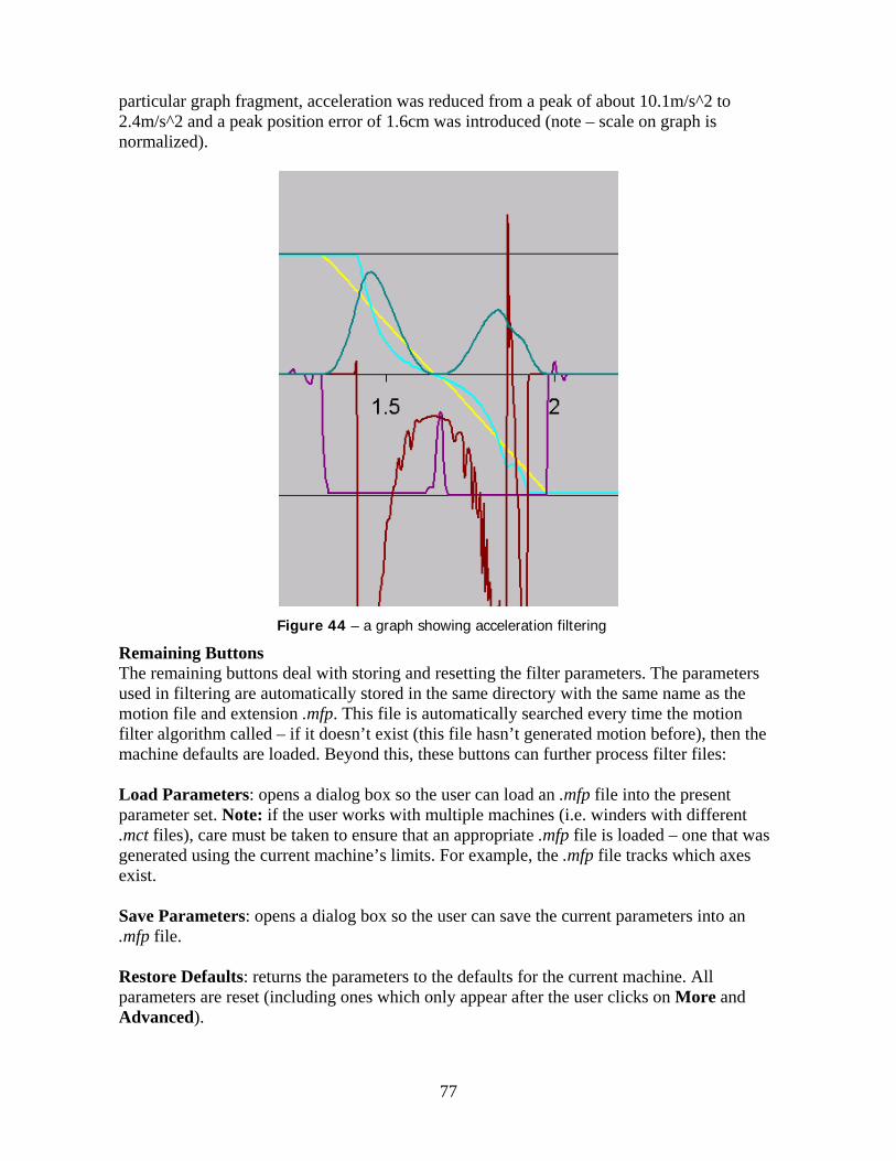
particular graph fragment, acceleration was reduced from a peak of about 10.1m/s^2 to 2.4m/s^2 and a peak position error of 1.6cm was introduced (note – scale on graph is normalized).

Figure 44 – a graph showing acceleration filtering

Remaining Buttons The remaining buttons deal with storing and resetting the filter parameters. The parameters used in filtering are automatically stored in the same directory with the same name as the motion file and extension .mfp. This file is automatically searched every time the motion filter algorithm called – if it doesn’t exist (this file hasn’t generated motion before), then the machine defaults are loaded. Beyond this, these buttons can further process filter files: Load Parameters: opens a dialog box so the user can load an .mfp file into the present parameter set. Note: if the user works with multiple machines (i.e. winders with different .mct files), care must be taken to ensure that an appropriate .mfp file is loaded – one that was generated using the current machine’s limits. For example, the .mfp file tracks which axes exist. Save Parameters: opens a dialog box so the user can save the current parameters into an .mfp file. Restore Defaults: returns the parameters to the defaults for the current machine. All parameters are reset (including ones which only appear after the user clicks on More and Advanced).

77

The final button is titled “More>>>” and expands the dialog box to introduce additional options.

14.2. Additional Filter Parameters After clicking the More button, an expanded list of filter settings is displayed (Figure 45). These are less frequently required, but can be used to tweak filtering characteristics in some cases. Only the “Reduce Mandrel Velocity Spike” option is selected by default. In general, these options may not be appropriate for all axes – the recommended use for each option is highlighted with a rectangle. The following topics cover the options in sequence.

Figure 45 – Motion Filter Parameter dialog box showing additional settings (after clicking on More>>>)

Lower Acc. – this first set of checkboxes allows the user to turn on an additional approximation algorithm which will attempt to further reduce the acceleration limit on a given axis until it either reaches 1/8 of its original level or the position error becomes excessive (a binary approximation algorithm is used). This can be very useful on the mandrel and carriage axis since these tend to have the greatest affect on machine vibration. If a motion profile consists of brief spikes in velocity, then this option is very effective, while it tends to have no affect on an axis which is already operating near its acceleration and velocity bounds over much of the trajectory. In such cases, if vibration is still excessive, the user should reduce an axis’ acceleration limit (which will reduce the axis’ velocity limit until a compliant trajectory is found). Min. Internal Err. – the second set of checkboxes applies a different criteria during position error compensation stage of the acceleration filtering algorithm. Normally, the algorithm attempts to minimize the end-point errors introduced during acceleration filtering – these are the errors which must then be removed through further maneuvering. The algorithm does not evaluate the error levels encountered within the filtered (i.e. constant acceleration) region. If this box is checked, after establishing the filtered region, the algorithm will also determine

78

the minimum and maximum position error encountered and adjust the start and end position to minimize these. In general, this will result in additional position error compensation maneuvers because the end-point errors will increase. However, for some maneuvers, this trade-off can be useful. This is especially the case on the carriage (and sometimes the cross-feed) axis if these are generating peak position errors at the ends of a bottle (which often tend to reduce clearance) – setting this box can reduce the peak errors which can yield additional surface clearance. The following graphs show such an example:

Figure 46 – shows two motion graphs indicating the effect of minimizing the internal position error of a high-acceleration region (Min. Internal Err. is turned on for the right graph)

The first graph shows a normal motion fragment, while in the second graph internal position error minimization it is turned on. The pink line represents the original position information while the purple line is the filtered position information. The blue-green line represents position error. As is clearly visible, the pink and purple lines cross each other more often when internal error minimization is turned on. Also, more residual error is introduced, so the axis is in error for a longer time, although this residual error is still quite small. However, the axis as a whole experiences significant improvement in peak position error. In this fragment, peak error is reduced from about 1.61cm to 1.16cm (note: the blue-green line is normalized and cannot be directly compared) – and for this particular trajectory as a whole, peak error was reduced from 1.92cm to 1.16cm and the crossfeed axis experienced a similar improvement from 0.68cm peak error to 0.36cm. When applied to an appropriate trajectory, this algorithm tends to increase velocity and position overshoot at the end of the axis’ travel – in the example case, the position went from 0.08cm undershoot to 0.96cm overshoot and velocity went from 1.8% overspeed to 3.8% overspeed (in both cases, some overspeed was needed to eliminate position error, although neither case came close to the 10% default margin).

79

Soft Vel. Enforce – Velocity enforcement takes place across all axes simultaneously – the violating axis causes the remaining axes to slow down. In this way, no position error is introduced. However, such enforcement can introduce significant acceleration spikes and velocity reductions on the other axes. In a few limited cases, it may be desirable to disconnect the axes during speed enforcement – for example, at the ends of a bottle, the payout eye must do a rapid rotation of up to 180 degrees while the other axes experience little motion. Depending on the payout system, there may be a significant level of error tolerance in this motion. Turning Soft Vel. Enforce on will allow the given axis to attempt to correct for speed violations without slowing down the other axes. In general, this introduces significant position error, and is not appropriate for the major axes. However, if significant, momentary misalignment of the payout system (i.e. eye rotation / eye yaw) does not adversely affect fiber path stability or cause problems in the payout system, it can improve program throughput on some files. It is best suited to files where motion nearly stops while the payout system rotates. If turned on, the user may select which portion of the overall position error may be “used up” during velocity enforcement (as opposed to acceleration enforcement). This value is unlikely to require adjustment. If velocity enforcement introduces a greater error, then the method fails and the axis reverts to “normal” velocity enforcement (i.e. across all axes). Reduce Mandrel Velocity Spike – Some mandrels (typically bottle winds) have a tendency to introduce velocity spikes on the mandrel axis due to rapid changes on the other axes. Such spikes do not significantly improve the program throughput and can be a source of significant machine vibration. Setting this option on will cause the software to reduce the velocity limit of the mandrel by a certain factor (based on the entry in: % velocity step) and check to see how much this extends a program’s execution time. If the change is minimal (based on the entry in: less than % acceptable growth per), then the procedure continues until the growth in time is too large. This is the only algorithm which is turned on by default. It rarely needs to be turned off unless there is some compelling reason to squeeze every last fraction of a second out of execution time.

14.3. Advanced Filter Parameters The dialog box (Figure 45) adds one button called Advanced. Clicking on this brings up the final group of parameters for motion filtering. These options adjust various parameters which affect the internal operation of the filtering algorithms. They generally do not require user adjustment, although they may improve performance in some cases. They fall into two categories – the first three parameters affect the oversampling algorithm while the next seven affect the acceleration filtering algorithm. Of these, the user will probably find the first set more useful. Some caution is advised when adjusting these parameters. If any set of parameters cause problems, click on “Restore Defaults” to return to a stable state.

80

The first three parameters establish how the oversampling algorithm operates. The first step in filtering is to oversample the original trajectory. This gives filtering finer control and is especially important for simple paths such as helixes where the original trajectory consists of very few points. The parameters are as follows: Max Evaluation Pts - this establishes the maximum number of trajectory evaluation points to use when filtering. Most modern computers can handle quite a large number of points for calculation, however, there are limits to how many points can be processed by Omniwind or Compositrak – see note below. On simpler files, this threshold is rarely reached, although with large files (and especially chained files), it can begin to lower the oversampling factor. Note that regardless of the number, the oversampling algorithm will never eliminate original points. In other cases, it will reduce the oversampling factor such that:

Original Points * Oversampling Factor < Maximum Evaluation Points

Oversample Factor - the original number of trajectory points is multiplied by this factor and new points are generated at equal intervals between the original points. If the trajectory has 3 points at t=1, 2, and 4 seconds and the oversample factor is set to 4, then the resulting trajectory will have points at: 1, 1.25, 1.5, 1.75, 2, 2.5, 3, 3.5, and 4. Information for these new points is interpolated from the original data. The default value is 10, which is reasonable in many cases. If a trajectory has a very limited number of points and the resulting filtered trajectory shows significant overshoot at transitions, then raising this value may improve results. Lowering this value will improve execution speed. Finally, if a trajectory is noisy (the acceleration axis has regions with very frequent and abrupt changes in acceleration which looks like noise on an oscilloscope) then this value should be set to 1 – oversampling will often generate even wilder oscillations in such cases. Pruning min dt - after filtering is complete, the algorithm will prune oversampled points. Points closer than this threshold (in seconds) are pruned (deleted) such that the final set of points will have an average separation of this value. Original points are never pruned. Setting this value very low (e.g. 0.0001) will effectively turn off pruning. A note on file sizes: Omniwind has a limited storage capacity for coordinates. The oversample factor greatly influences how many points are in the final file. Due to the integral nature of the oversample factor and pruning (see below) the final number of points in the filtered .mmt file is generally less than the number entered at Max Evaluation Pts. The actual number of points in the file can be determined from the motion graph. On a 4-axis machine, Omniwind can process about 1,400 coordinates per file. Omniwind will warn the operator that a motion file is too large. If so, the user may adjust the values in this dialog box, or if the original data was already too large, the user may need to reduce the path thresholds which generated the original data: “Cyl. Section Threshold” and “Dome Section Threshold” are used for bottle winds and non-linear winds, and “Path File Threshold” for helixes.

81

The final seven parameters control how the acceleration filtering algorithm works. The algorithm consists of two parts – first scanning the trajectory for larger trends and evaluating and adjusting these. Then rescanning both these regions and the entire trajectory with a small window, looking for local acceleration violations. The first part scans for acceleration regions based on moving pointers along the trajectory and checking if certain conditions are met. The pointers track points of minimum and maximum velocity for a particular acceleration region. As long as a set of conditions is met, one pointer is dragged along until a threshold condition is met. If this threshold is not attained and the general trajectory trend changes (e.g. acceleration changes to deceleration), then the pointers are reset and the process continues. Once this threshold is attained, a region is considered to exist – it will continue to grow until another set of terminating conditions is met. Once all regions are established, the region with the greatest velocity change is checked for acceleration violation. If found, the region will continue to grow until its starting and ending velocities divided by its duration is below the acceleration threshold – then a straight-line acceleration is applied between these points. The growth of the region is set-up to minimize error at its endpoints (unless the “Min. Internal Err.” checkbox for the given axis is set), and a compensating maneuver at low acceleration and velocity levels is superimposed to eliminate this residual error.

The second type of scan passes a window over the trajectory. The algorithm verifies that the acceleration within this window is below the given threshold. If so, the window continues moving the length of the trajectory. Otherwise, the local region is adjusted in a similar manner as described above. The following parameters affect this process:

82

Minimum Traject. dv - establishes the minimum change in speed (dv) over an entire trajectory before any acceleration enforcement occurs. This value is given as a factor of the axis’ speed limit. The value prevents trajectories with zero or near-zero speed change from causing problems during enforcement due to floating point issues. Trajectories with such minimal dv’s on a particular axis often require no filtering, even if they have significant acceleration due to noise. The default setting of 0.02 rarely requires adjustment, although if a particular trajectory has little dv but unacceptable noise, the value can be adjusted downward which may trigger acceleration enforcement. dv Threshold - establishes the threshold at which an acceleration trend is established. This is given as a factor of the total velocity change in the trajectory (i.e. maximum minus minimum speed). An acceleration/deceleration trend must cover at least this magnitude velocity change before being considered a region. dv Turnaround - once a region is established, this value affects determines one of the two terminating criteria. If acceleration changes polarity and the change in velocity exceeds this magnitude (defined as a factor of the total velocity change in the trajectory), then the region is fixed at its current start and end points. Accel Hysteresis – This parameter has two functions – before a region is established, it establishes a minimum acceleration rate between start and end points. If this rate isn’t met, the region collapses. Once the region is established, its function is reversed – this minimum acceleration rate must be met between end point and the new evaluation point, otherwise the region won’t grow. It is defined as a factor of the axis’ acceleration limit. Min Shoulder – This parameter establishes the second condition for terminating an acceleration region – the width of its shoulder: if a velocity plateaus (i.e. it cannot grow due to the hysteresis defined above), and this plateau exceeds the duration of the region times this factor, then the region is fixed. For example, if an acceleration region has a duration of 0.3 seconds and Min Shoulder is 0.2, then the region would be fixed if its shoulder exceeds 0.06 seconds (assuming the turnaround condition didn’t kick in prior to this). Local dv Threshold – the equivalent to dv Threshold for the windowing acceleration algorithm. This combined with the acceleration limit determines the minimum width (in seconds) of the scanning window. This scanning window then slides along the trajectory and if the average acceleration within any given scan exceeds the limit, then the region is again expanded and acceleration reduced in the same manner as described in the introduction above. In general, dv Threshold, dv Turnaround, Accel Hysteresis, and Local dv Threshold are adjusted in tandem, because they closely interact. Reducing them all makes the acceleration filtering algorithm more sensitive to minor velocity changes, while large values require larger changes before filtering kicks in (which can be more effective at establishing trends on noisy trajectories – in some cases, it can be better to use large values for all of these except Local dv Threshold which is left small to filter noise).

83

Accel Region Growth – Acceleration regions grow in order to reduce the acceleration level within them. Once this level is acceptable, this parameter establishes if they can grow further in order to reduce residual error (the remaining position error at the endpoints). The algorithm will check the resulting residual error if the region grows at either extremity by one sample. If this error is less than the current residual error, growth continues until the duration of these added segments exceeds this factor of the initial region’s duration. For example, if an acceleration region requires 0.5 seconds to obtain an acceptable acceleration level, and Accel Region Growth is set to 0.2, then it may grow up to 0.1sec more as long as such growth continues to reduce residual position error (note that this does not ensure that peak position error within the region is also minimized – the affect on it is indeterminate).

14.4. Using Excel® to Graph and Compare Filtered Motion The filter algorithms include code to support detailed graphing in MS-Excel®. After filtering is complete, the code generates a text file called “finalstg.txt” (final stage) together with the motion (.mmt) and filter parameter files (.mfp). These are all placed in the same directory. This file contains time, original position, and filtered position, velocity, and acceleration information for each axis. A Visual Basic® script has been written (in Office 2000®) which takes this data and automatically generates appropriate graphs for each axis. This is stored in a file called: “GraphMotion.xls” which is kept in the Composite Designer directory (e.g. “c:\Program Files\Composite Designer”). Here is an example graph:

Figure 47 – Shows a typical motion graph detailing the effects of the most recently run motion filtering operation

84

The graph is useful for both understanding the operation of the filtering algorithms and to analyze actual machine motion in physical units – for example, to verify velocity and acceleration limits and, in particular, to establish the size and location of position errors. The legend for each axis also indicates the total number of points (shown on same line as position error) which is useful for evaluating file size with respect to Omniwind. In typical use, the user may alter a few filter parameters and simply re-execute the macro in Excel to see the changes (note: the original graphs will be replaced, except for any user-modifications to the graph’s format). To store a particular graph, use “Save As…” rather than Save. GraphMotion.xls is write-protected to prevent the original spreadsheet contents from being accidentally overwritten. If the file ever damaged, users can obtain the original file off the Composite Designer CD. To use this functionality, the user should open “GraphMotion.xls”. Depending on security settings, the user may need to enable macros to use the script. Once open, click on the menu heading: Tools | Macro | Macro… In the dialog box which appears, click on the macro “ProcessFile”. To study position error in detail, the user may wish to execute the macro: “ShowPosition” – which removes all series except for position and position error (note – to restore the original graphs, the user must re-execute “ProcessFile”). The macro will now ask for the required data file (finalstg.txt). This allows the user to use different directories and also store multiple text files (which are relatively compact, compared to the large files generated once graphing is complete). The macro will then analyze the given data and extrapolate information about machine motion prior to acceleration filtering. The resulting graph will display position, velocity, and acceleration for both the pre- and post- acceleration filtering (unfortunately, plotting data prior to velocity enforcement would result in different time values). The graph also displays the magnitude of the position error at any given point. The graph is normalized such that filtered motion parameters occur between –1 and 1 (the corresponding values are shown in the legend). The same scale is applied to pre-filtered motion – which has little affect except for acceleration. The user can still use all Excel capabilities to further adjust the graph – such as turning off individual lines or adjusting axis scales – or generate new graphs (by studying the format of the graphed data itself. The standard graphs plot data from columns M through T). A few notes: in general, a graph should never have position error or velocity levels which exceed the entered limits. In some cases, acceleration values may still experience very brief spikes – although these should occur over minimal changes in velocity (often where data points are extremely close together and a minor change in velocity occurs). The graph will, of course, show the peak value, although the user should focus on the sustained peak acceleration. The user should verify that there is no significant change in velocity occurring at the acceleration spike. Adjusting the advanced filter setting Local dv Threshold can reduce this effect.

85

Also, the motion shown in the graph may not fully agree with motion displayed in Composite Designer due to differences in the use of approximating splines. This will appear in Composite Designer in the form of some position oscillation before any major change in velocity and is dependent on the distance between samples. In general, machine motion will follow the profile displayed in Excel, unless the user does some subsequent editing of the data in Composite Designer and saves this new motion.

14.5. Chain File Filtering Issues The filtering algorithms are usually capable of smoothing chained files as well as individual segments. Generating feasible motion in these cases is more challenging. At segment boundaries, position and velocity values must align to both the next segment and to the start of the present segment (if the segment is periodic – generally the case except for single pass circumferential winds). To achieve this, both the transition-path generating code and the filtering code inserts copies of current segments in order to establish a transition region which does not need to meet the same criteria of periodic continuity. Note that the algorithm keeps track of the total number of cycles of a periodic segment and adjusts this number as required if a segment is copied. From the user’s perspective, the steps for generating smooth motion are nearly the same. At present, there is only one set of filtering parameters (they cannot be varied from segment to segment). There are no special considerations for any particular settings. Filtering algorithms are first applied to each segment in the chain, and then additional filtering occurs at segment boundaries. In this way, one segment does not have a significant impact on the next (e.g. the approximation algorithms may lower the velocity limit for a particular axis in a particular segment if no solution is immediately found – but this would not affect the velocity limit on that axis in neighboring segments). In most cases, the user is likely to generate motion based on a transition path. In other words, Composite Designer will calculate a fiber path which connects the end points of the chained segments and use this to generated the required motion. In this case, the user should build the chain file by inserting the original .mmt files, not any filtered files. For example, to chain two segments built using the names BottleHelix and BottleCirc, the user should chain together “BottleHelix.mmt” and “BottleCirc.mmt”, not “BottleHelixflt.mmt”… This is because the path files (.pth) are stored under the original file name and these are used to generate actual motion, the data in the .mmt files is mostly ignored. Once the user generates motion, two files are generated – the original motion file with the user’s given name (e.g. “BottleChain.chn”), and a filtered file with “flt” appended to the filename (“BottleChainflt.chn”). If transition sections are based on motion rather than path, then it is not critical to use the original (unfiltered) .mmt files, although this is still the recommended method (it only applies filtering once to the final file; multiple filtering levels generates cumulative position error which would be difficult to evaluate).

86

14.6. Some Tips on Motion Smoothing Motion smoothing / filtering often produces reasonable results, even with a fairly fixed set of parameters. If a particular machine is largely used to make similar parts, it may be advantageous to save a motion filter parameter file in a fixed location and then load the file whenever starting a new project (rather than reverting to the machine defaults). The filtering algorithms do have some limitations – a primary one is that they only generate files which are equivalent to a maximum axis rate envelope (i.e. no constant mandrel speed or constant fiber speed). There are also a few geometries for which the current approximation algorithms have difficulties – generally low-angle bottle winds. In some cases, the resulting motion is excessively slow in the dome region. The user may wish to directly edit the rate envelope in the dome region to reduce wind times. Another issue is that the algorithms do not currently carry out true “filtering” (e.g. low-pass). If a particular motion file is noisy but without excessive acceleration levels, then the output file can also be noisy. If the resulting motion is unacceptable, the entire axis can be selected and smoothed. See page 56. A nice benefit to simplify further manual editing is that all output files have a fixed rate envelope. The following tips may be of assistance when generating motion and smoothing it: Issue: After filtering, motion is still too abrupt. Consider: Lowering the acceleration of the offending axis. This has a tendency to increase program run-time. Also consider use of the Lower Acc. option for that axis (see page 78). Issue: Motion profile has some irregular or unexpected portions. Consider: this can have several causes. Because of the mathematical transformation involved in converting a fiber path to a machine motion trajectory, some points in a program can require the machine to move a great deal while the fiber’s point of contact remains nearly stationary, while in other cases, many fiber path points resolve to the same machine coordinate. Because of this, regions of the motion file have very few points while other regions have many points at nearly the same location. This is particularly the case in programs with low fiber angles and also during fiber rotation at the end of a bottle. The user may try to use a smaller value for the path thresholds during generation of the original file to increase the number of samples – the relevant parameter depends on the fiber geometry – “Cyl. Section Threshold” and “Dome Section Threshold” are used for bottle winds and non-linear winds, and “Path File Threshold” for helixes. The issue above can cause some irregular motion due to spline approximations. The software uses cubic splines to interpolate motion between points. In regions where the distance between samples changes abruptly, the spline can oscillate. These are visible when the user loads an .mmt file into CD – look for regions of oscillations which don’t follow the motion points. Figure 48 shows an example.

87

Figure 48 – shows how spline curves can introduce oscillations

Here the pink line is displayed by Composite Designer while the blue dotted line is the motion which might be expected. When this data is then fed to the filter, the oversampling algorithm will add points which follow these oscillations. In such cases, setting the oversampling factor to 1 (turning it off) will often help. Issue: Crossfeed motion is irregular on a chain file Consider: The different files in the chain file have different mandrel geometries – in particular, the mandrel radius changes between files. Ensure that all files use the same mandrel geometry.

88

15. Chain / Transition Files The final wind program module in Composite Designer (CD) is the chain/transition wind. These winds allow users to connect several files together and execute them in sequence. In addition, transition motion can be automatically generated to assist with the generation of smooth and stable motion from the end of one file to the start of the next. As with all wind files, the first step is to create a new program via the File | New | Chain/Transition Wind command. This brings up a window (Figure 49) allowing the user to enter a list of files to be chained together.

Figure 49 – the Chain / Transition entry window

To add a file to this list, the user first right-clicks the mouse over the bulls-eye target. This brings up a sub-menu which has entries to Insert and Delete Segments. Clicking on insert brings up an open-file dialog box where the user can select an .mmt file (or Compositrak-based .seg file) to be inserted (note that existing chain files cannot themselves be chained). To continue adding files, first left-click on the file to be deleted or on the file in front of the insertion point (or the bulls-eye if inserting a new first file). This is required to select the insertion point. Then right-click and use the Insert Segment command, etc. To delete a file, again, first left-click on the file and the right-click and select the Delete Segment command. In this way, a complex chain file can be generated fairly rapidly. One important concept in chaining files together is the transition segment. Between each segment, Composite Designer will automatically generate transition motion. The user can select one of three possibilities via the Output Options portion of the window (the fourth

89

option – Build CTS File Directly deals with Compositrak controls). The following sections deal with these in sequence.

15.1. Transition Motion Files If this option is selected, Composite Designer will generate motion which connects the final state of one segment with the starting state of the next segment by directly extrapolating a trajectory based on various acceleration and velocity limited criteria (i.e. connect the velocities and positions of all axes). The intermediate path is not based on any consideration of either mandrel shape or fiber stability. This process tends to work well for connecting relatively short gaps in fairly similar winds. If this method is selected, the user would enter four parameters in the lower window portion as follows: Transition Evaluation Points – this parameter is fairly clear. The user enters a whole number and the software will extrapolate this many points in each transition region to be calculated. Transition Region Rate – this applies a limit similar to a wind angle to the transition region – defined as limiting the carriage speed vs. mandrel speed (i.e. number of carriage position units per revolution of the mandrel). Payout Eye Tooling Offset – here the user can add an additional fixed offset to the crossfeed. This might be used if the designer believes clearance in the transition region to be inadequate (since transition motion does not consider actual mandrel shape, only smooth machine motion). Note that this offset is applied to the entire file, so it may cause problems in terms of path stability on some shapes. Transition Motion Tolerance – this is a type of unit-less “smoothing” factor. The closer to zero, the more abrupt the motion in the transition region. High values allow acceleration to take place over the entire maneuver. Typical values are between 1 and 100.

Figure 50 – the Chain/Transition dialog box allowing user to set segment flags

90

Once the user has inserted all the files to be chained and set all the necessary parameters, he/she can click on the Calculate button. The user is prompted to enter a filename. Next, a dialog box appears (Figure 50) allowing the user to select the number of circuits in the wind and also set the flags for each segment boundary (these flags apply to the start of the segment). Note: this dialog box appears for all types of chained motion files. The following flags can be set:

- Auto Find Path – only available on transition segments – this will automatically stop the machine, perform a Find Path for the next segment, and start up again (unless the Hold flag is also set). The motion in the transition segment is essentially ignored.

- Auto Hold – automatically holds the machine at the segment boundary. The user will need to release the hold condition to continue.

- Mandrel Offset – when set the mandrel will not move to the zero degree location at the beginning of the segment. If set in the first segment of the chain, then the mandrel will not rotate forward to the next zero location during the initial find path. Between segments, if not set then the machine will stop and the mandrel will rotate forward. For this reason, it is a good idea to set this flag in all segments, especially after the first.

In general, if the user wants a file which will execute non-stop from start to finish, they should make sure that Auto Find Path and Auto Hold are cleared in all segments and the Mandrel Offset is set in every segment (it can be cleared in the first segment). In addition to segment flags, this dialog box is also used to override the current entries for number of circuits in a given segment and also the names of each segment. Doubling the number of circuits effectively doubles the number of layers a particular segment will generate. The segment comment is the name which appears in Omniwind while executing the part. All of these entries can also be set later when editing motion (see section 13.5). If the user is satisfied with these entries, he/she can press OK and motion is generated. As with other types of wind, a dialog box appears allowing the user to filter the resulting motion (see chapter 14). This may or may not be necessary if the underlying files were already fairly smooth – the user can examine the resulting motion and decide. Transition Motion Files can combine any type of wind, although they tend to work best on winds which already mesh well (i.e. no major change in fiber angle, end points already closely aligned). In some cases, they are the only option – e.g. when chaining zero degree winds. They directly incorporate their component motion files, meaning any already edited motion is left unchanged.

15.2. Transition Path Files This is the other major transition option, and also the typically more complex and powerful one. In this case, CD ignores the data contained in the motion files to be chained. Instead, it goes and fetches path file data from .pth files with the same name and uses these as the basis

91

for generating the chain file. It uses this path data to build a model of the mandrel, and, in turn, uses both of these to generate a transition fiber path which connects the end of one program to the start of the next. Finally, it takes this resulting fiber path and generates machine motion, in a similar manner to how motion is generated for bottle and non-linear winds (but differently from circumferential and helical winds). In general, transition path files have a much better chance at combining diverse segments with stable transition regions – going from a low-angle bottle wind to a final outer hoop wind is relatively straightforward. Because it works with path files and generates a transition path, this option requires that the .mmt files to be chained are accompanied with .pth files of the same name. This implies that even if the user is generating filtered motion, instead of chaining the filtered motion files, he/she should chain the original files (without the appended “flt”). Filtering can then be applied to the resulting motion. It also implies that transition path files cannot be used for zero-degree winds because these directly generate motion without creating an intermediate fiber path. Two parameters are set for this type of chain wind:

Transition Region Threshold – this should set how frequently (in terms of linear fiber path) the software generates points in the transition region, although it is not fully implemented at present. The user may need to try a few values for the software to accept the wind parameters. Transition Region Rate – this applies a limit similar to a wind angle to the transition region – defined as limiting the carriage speed vs. mandrel speed (i.e. number of carriage position units per revolution of the mandrel).

Once the user has entered all the files to be chained and set the above parameters, clicking on Calculate will generate the new path and display the chain/transition feedback dialog box (see previous section for information about its contents). One difference, if an intermediate file includes a bottle or non-linear wind, the user will receive some information about slip factors in the transition regions. Values near zero are more stable. The user may wish to adjust the transition region rate to improve stability. Once the user is satisfied with the settings in this box, he/she clicks ok and is prompted to enter a filename. At this point, a new path has been generated, meaning the user can generate 3-D views of the part (see chapter 11). Finally, when satisfied, the user would click on Calculate | Machine Motion. This brings up the standard motion generation dialog (see chapter 12).

15.3. Do Not Transition option As a final option, the user can have the software simply chain files together with no calculated, intermediate motion. The process is similar to that for Transition Motion Files (see section 15.1) except no parameters are entered on the first screen. This motion option is typically used in the following two cases: either the existing motion matches up extremely well (e.g. various helical winds with only an angle variation) or the operator intends to stop

92

the machine between layers, tie off the fiber, and do a find path. In the latter case, the utility of the chain file is primarily simplifying the execution of multiple layers. If the layers mesh well, the user could use similar segment flag settings as with other chain-wind types (i.e. only set the Mandrel Offset flag). Otherwise, flags should be set such that the machine holds at the end of each layer. Even though no motion is implied, due to software constraints, there will actually be a miniscule motion segment inserted (of about two degrees of mandrel rotation). This can cause a need for motion editing if an axis other than the mandrel is moving during the transition.

15.4. Chain File Tips and Troubleshooting When generating path-based chain files, it is important to use “equivalent” mandrels for each segment. This is because the software uses path file coordinates to reconstruct a composite mandrel shape of all the different layers. For example, even slight differences in part diameter can result in highly erratic crossfeed behavior because the mandrel surface will consist of tightly spaced points with varying diameters resulting in a very jagged part surface. Some tips for obtaining a consistent mandrel are:

- Always use the exact same bottle specifications for different layers (i.e. use the same bottle shape type, the same diameter, cylinder length, same dome width, etc.). The same applies to non-linear winds.

- To overlap a circumferential wind on a non-linear wind, use the circumferential option of the non-linear wind.

- To overlap a circumferential wind on a bottle, set the start and end coordinates appropriately. For example, if a ellipsoidal bottle has a left and right dome width of 5 inches and a cylinder length of 20 inches, the circumferential wind’s start and end coordinates need to lie within 5 and 25 inches.

This restriction only applies to path-based chain winds. The other modules do not attempt to reconstruct the mandrel shape. If a particular segment / layer is to be repeated several times in sequence, it is usually a better idea to modify the number of circuits instead. This avoids generating so many transition regions and simplifies and additional editing. It also reduces the final file size (which can give Omniwind more room for other tasks or adding more layers to the wind). Setting the number of circuits per segment is discussed in section 15.1. When connecting highly dissimilar segments, it is usually better to have their motion start at opposite ends of the part. For example, when chaining a low-angle bottle wind to a circumferential wrap, the user would typically start (and end) the bottle winds at one side of the mandrel and then begin the circumferential wind at the other. This makes it easier for the software to find a reasonably stable path. This left-right setting is typically made when selecting a path or when entering part parameters. See the individual chapters of the wind-types in question for more information. In rare cases, the opposite case may work better (i.e. both segments ending on the same end of the mandrel) so the user may want to experiment with these settings.

93

16. Auxiliary Output Files So far this book has focused on the various modules and methods to take a part design from concept to motion file. In addition to coordinating motion to generate a part, Composite Designer and Omniwind support additional external controls. This auxiliary output module allows the user to specify logical conditions which trigger voltage signals to other devices. Auxiliary output control is encoded in an .aux file. Whenever Omniwind loads a motion file, it searches for a similarly named file with the .aux extension and automatically executes the two in tandem. The first step in creating an .aux file is the command File | New (or the toolbar button ) and then Auxiliary Output Files. This brings up the following window:

Figure 51 – the auxiliary output condition entry window

The window is divided into several regions. At the top is a list-box which allows the user to enter various conditions which should trigger a particular event. Below this are buttons which define the polarity of the output and the Boolean operator (AND or OR) to use when combining the conditions defined above. The center of the window consists of a large set of

94

buttons allowing the user to select a particular output and timer condition. The lower window region allows the user to set a starting value for the current countdown timer. Finally, the user can select metric units by checking the box at the bottom of the window.

16.1. Digital Auxiliary Outputs If the user only needs fairly simple trigger conditions, the first step is to click on the auxiliary output button to be edited. At this point, the user may select default behavior for the output by clicking on the appropriate selectors just under the list-box. The Default State is the output state when the auxiliary output’s condition evaluates to false. On implies voltage is present at the output (typically +24VDC). When the condition evaluates true, the output state is the inverse of the default. The Error State is the output’s state whenever the control is in E-stop. This overrides all other conditions. The final selector, Boolean Operator, establishes how the conditional statements are combined – either via AND or OR. All statements are combined with the same operator. Even though more complex combinations are not available, by selecting conditions and default states appropriately, and by the use of Boolean math, fairly complex conditions can be generated. The user could now enter logical conditions in the top window. The Auxiliary Output Menu | Add Condition… menu command is used to do this. It brings up the Add Auxiliary Output Condition dialog box (Figure 52). Here, the user can specify a particular condition which should form part of the logical statement which triggers the output.

Figure 52 – the dialog for adding a condition to an auxiliary output

A single condition consists of a data source (the quantity to be measured), selected via the drop-down list-box at the top of the screen, and two values defining the range over which the quantity evaluates to true. One important note about ranges: they always define a closed region. As such, their starting and ending values are essentially interchangeable. For example, if a particular axis has a position condition with a starting value of 30 inches and ending value of 20, the condition will evaluate to true as the machine moves from 19.9 inches to 20.1.

95

The following sources are available for measurement: Axis position – allows the user to enter a position range for any available axis. When the axis falls within this range, the condition evaluates to true. The range will depend on the axis and unit system. For the rotary axes (mandrel, eye-rotation, and eye-yaw), the units are in degrees. The mandrel is a somewhat special case since it continuously rotates in one direction. For auxiliary output purposes, it is absolutely referenced to the axis’ home position and its value will rollover to lie within 0 and 360. For linear axes, the units are in inches or mm and are based on the coordinate system as displayed to the operator of Omniwind (see chapter 17, especially page 116). Circuit number – within each segment of a particular program, this condition will evaluate to true if the winder is currently executing a circuit within the entered range. The range includes the start and end circuits, so a start value of 3 and end value of 6 would evaluate to true over a range of 4 circuits. In a chained, multi-segment program, this condition can evaluate to true within each segment (if that segment includes circuits within the specified range). With chain programs, see the note in the box below. Segment number – for multi-segment programs, this condition will evaluate to true if the currently executed segment is in the specified range. As with circuit number, the range includes both start and end segments. See note below.

Note: When using segment and circuit based conditions with any chained motion file, the user should first examine the motion file to determine the appropriate circuit and/or segment number. This is because the chain module and the filter module can generate new segments and make single-circuit copies of individual segments in order to smoothly link motion at segment boundaries. This affects both the total number of segments and the number of circuits within a segment. To verify these numbers, the user would open up the motion file and examine its motion table (with the line-graph display, very short segments may not be visible). The first column shows the segment name and number and the number of circuits within the segment. For more on motion table editing and navigation see sections 13.5 and 13.6.

Process time – this is the time that a particular part program has been executing in seconds. Execution time does not include time spent: in hold, during find-path, while jogging an axis, or while the machine is enabled but not actually running the program. It includes time executing at a zero or negative rate. Process time is real time; it is not scaled by the current execution rate. Process time is reset when a program is loaded and also when a program is run to completion and then run again without reloading. Axis velocity – allows the user to enter a velocity range for any available axis. The range will depend on the axis and unit system. For the rotary axes (mandrel, eye-rotation, and eye-yaw), the units are in rpm. For linear axes, the units are ft. / min or m/s. They are based on actual velocity of the axes during the wind as displayed to the machine operator, not the value programmed into the wind (i.e. they incorporate how fast the program is executing). They also incorporate polarity, so a range of 1 to 2 m/s would register as true on the carriage if the

96

machine were in that speed range and heading towards the tailstock, while a range from -0.05 to +0.05 would register as true while the axis is stopped or near a stop. Timer – allows the user to add a condition based on if a particular countdown timer is within a certain range. See below for more information on timers. In some cases, a user may wish to create a more complex condition. This can be accomplished by repeatedly adding output conditions. The entire group of conditions can be combined using a logical AND (i.e. all conditions must be true for the result to be true), or a logical OR (i.e. one or more conditions must be true for the result to be true). At present, condition statements cannot be directly edited, only added or deleted.

16.2. Analog Auxiliary Outputs In addition to digital auxiliary outputs, some machines offer up to eight analog outputs as well. These are configured in a similar manner to the digital outputs just discussed. All conditions and ranges have the same meaning. Rather than simply evaluating true or false, each condition includes an output value – entered under Magnitude in the Add Auxiliary Output Condition dialog box (Figure 52). If a particular condition triggers the output, then the voltage is typically in the range of +/-10V corresponding to magnitude entries of 100% and –100% (although this may vary with any custom analog output circuitry). The actual state (i.e. voltage) of the analog output depends on various factors, due to the possibility of different magnitude entries for different conditions. One thing to bear in mind is that condition lists are evaluated sequentially from top to bottom in the same order as they appear on the entry screen. If the machine is in E-stop, and the Error State of the output is set to On, then the output maintains its most recent setting. If the Error State is off, then the output is turned off (0V). If the machine is not in E-stop, then the Default State setting becomes relevant. It must be set to off; otherwise the output is set to 0V (0%). If the machine is not in E-stop and the Default State is off, then analog conditions are evaluated. The output state depends on the Boolean Operator used. If the operator is AND, then all conditions must evaluate to true and the output will assume the magnitude of the final entry in the condition list. Otherwise the output will be 0V. If the operator is OR, then the output is set to the magnitude of the final condition which evaluates to true. For example, given the following machine state and condition list:

97

State:

Mandrel is at 39rpm and 150 degrees and process time is at 74.500seconds.

Conditions (in sequence) for Analog Output 1:

Mandrel velocity between +10 and +50 rpm, magnitude: 50% Mandrel position between 0 and 180 degrees, magnitude –50% Process time between 70.000 and 74.125seconds, magnitude: -100%

Boolean Operator: OR

In this case, the output will be at –50% (typically –5V) and is established as follows: Condition 1 evaluates true, output is tentatively set to +50%. Condition 2 also evaluates true, output tentatively –50%. Condition 3 evaluates false. Since there are no more conditions, the output is the last accepted value of –50%. If no condition is true, then the output is set to 0%. A simple way to alter this would be to set the first condition to a statement which would always evaluate true (e.g. process time between 0 and a 10,000,000 seconds) and set the magnitude of this entry to the desired “default” output value. While the user can use AND blocks to establish fairly complex conditions for a particular output magnitude, the use of OR blocks is often much more flexible for analog outputs. It allows the same output to assume many different output levels corresponding to different machine conditions.

16.3. Use of Timers A different type of “output” is a program timer. It does not generate a physical output. Instead, it generates an internal logical state which can be used by the condition lists of other outputs (including other timers). For the most part, the timer output can be thought of as another measurable quantity that is triggered in a similar manner to a digital auxiliary output. The user can set error (E-stop) and default state, a Boolean operator, and a list of conditions which are evaluated to control the timer. While other outputs always reflect the state of their condition list, a timer output is triggered when its condition list evaluation state changes from false to true. At this point, the countdown timer will load the value recorded in the Timer Output Setting box (see Figure 51). The timer will now start to count down. If the counter reaches zero, it stops. If the underlying evaluation state remains true or switches to false or remains false, these all have no effect – the timer will continue to count down to zero and then wait. However, if the underlying state switches again from false to true, then the timer is reloaded with its starting value, even if a previous countdown did not complete. For example, if a timer has a condition list as follows:

Mandrel position: range 0 to 180 degrees

98

and:

Timer Output Setting: 5.100 seconds then every time the mandrel moves from 359.9 to 0.0 degrees (or from 180.1 to 180.0 if moving backwards), the output condition will trigger true and the counter is loaded with 5.1 seconds and will start to count down. Now if auxiliary output 1 has the condition:

Timer 1: range 0.100 and 5.100 seconds Then it will evaluate true whenever the timer is counting down (except for the last 0.1 seconds). In practical terms, if the mandrel is moving forwards, auxiliary output 1 will go to true every time the mandrel hits the zero position. If the mandrel is spinning fast enough to complete a revolution in under 5 seconds (12rpm), then auxiliary output one will always be true. A few final notes: after entering a value in Timer Output Setting box, be sure to press the Set button, otherwise the value is ignored. Also, timers continue to evaluate in all conditions, even if the machine is stopped.

16.4. Final notes on auxiliary outputs While this chapter has covered the steps involved with generating auxiliary output programs, there are various aspects of computer operation and program structure that can affect the operation of the outputs. From power up until a motion file with auxiliary outputs is loaded, analog and digital outputs are set to 0V•. After Omniwind exits, analog outputs may maintain their previous state, although this depends on any external circuitry. If a motion file without auxiliary outputs is loaded, the outputs retain their last state. Once a file with auxiliary outputs is loaded, auxiliary output conditions are evaluated during each update cycle of Omniwind’s motion control board – about 1,000 times per second. If the machine is in E-stop, then all outputs have their E-stop condition. Otherwise, all conditions are evaluated regardless of current operating state. This implies that conditions, timers, etc. are checked and updated while the machine is idle, while the operator is jogging the machine, during a find-path maneuver, and, of course, while the machine is winding a part. Auxiliary output programs are executed by the motion control card within the embedded PC which runs Omniwind. Like Omniwind, their execution is independent of Windows. However, they do share memory space with the program being executed, so with complex parts and complex condition lists, it is possible to run out of memory. Omniwind will warn

• Behavior may be different for versions of Omniwind prior to 3.0. In all cases, if output condition is important before or after executing the motion file, the user may wish to verify machine behavior.

99

when this is the case. In general, the user is likely to return to edit the motion file to reduce the total number of motion program coordinates to free up memory for auxiliary outputs. Finally, while auxiliary outputs are evaluated on every update cycle of the motion card, they are not intended to be used for high precision requirements. In particular, some conditions may be prone to noise – especially axis velocity. This is due to the fact that axis speeds are rarely 100% constant. As an axis accelerates past a threshold value, the resulting, calculated velocity will often oscillate between true and false states depending on the discretely measured distance covered over the course of one cycle.

100

18. Digital Tensioning Some McClean Anderson winders include an optional, digital fiber tensioning system. This gives the designer / operator excellent control of fiber tension during a wind. Digital tensioners also provide great flexibility through features such as remote programmability via off-line software as well as from the operator console of Omniwind (see chapter 20 and section 17.10). They also offer unlimited fiber take-up capability. Tensioner operation is described in this chapter. One note: the terms “motor” and “tensioner” are used interchangeably to designate an individual tensioning unit within a tensioning system.

18.1. Safety Safety is a primary concern in the design, manufacture, sale, and use of McClean Anderson winders and digital tensioning systems. We would like to remind users of basic safety rules using a tensioning system. Tight, moving fiber poses a significant hazard to machine operators and bystanders and failure to follow these guidelines can result in serious injury or death. IT IS ESSENTIAL that everyone involved in the operation, and maintenance, of this equipment is aware, concerned, prudent, and properly trained in safety. Following these safety rules, as well as others identified in the owner's manual and in product safety signs, will help minimize the possibility of accidents and increase productivity:

• Before operating a tensioning system, an operator must read and understand all of the information in the owner's manual and the safety signs attached to the product.

• Wear appropriate safety gear for the task at hand – including: gloves (for fiber and

resin protection), safety eyewear, and possibly respiratory protection.

• Be sure the emergency stop button on the tensioning unit is pressed whenever changing or getting close to the fiber path or spools.

• Always check surroundings before turning on the tensioning system. Verify that there

is no one working around the creel or in the fiber path.

• To change a fiber spool during a wind, follow these steps (refer to Figure 64 through Figure 66 for machine photos): 1) Turn individual tensioner enable switches off and place the tensioner and winder

into E-stop by pressing the appropriate buttons (the winder can recover from this without losing position)

2) Put on appropriate gloves before handling the fiber. 3) Open the creel door and turn off the air switch on the spool to be changed 4) Replace the spool making sure that fiber pays out on the correct side

129

5) Thread the fiber correctly over the load cell and the remaining distance to

complete any splice – try to avoid letting the fiber get too loose (the tensioner motor/spool can be backed up by hand after the splice is done and before restarting the machine)

6) Turn the air back on and close the creel door 7) Enable the tensioner system and turn the individual tensioners back on; resuming

the wind typically requires clearing E-stop (pulling out the button and pressing “Reset”), then performing a Find Path, and finally using Enable and Inc to resume winder motion

Warning: changing an individual fiber spool without putting the tensioner into E-stop (i.e. maintaining tension on the remaining spools) is hazardous and not recommended.

• Do not operate tensioner when fiber redirect pulleys are loose, worn or sticking.

• Never touch the load cell or manually move the spool when the tensioner is on

• Do not bend or put a heavy load on the air-chuck assembly.

• Do not directly wrap the air-chuck with fiber, it could cut or damage the air-chuck

• Never inflate an air-chuck without a spool – this can damage or rupture the bladder

• Use extra caution when winding with carbon fiber, which is very conductive. It is

critical that the creel doors remain closed while winding it. Failure to do so could cause electrical system short or failure of surrounding equipment. All electrical systems surrounding the tensioning system must be sealed.

18.2. Tensioner Overview Figure 64 shows a tensioner control panel with the various components labeled. Once power is applied and the tensioner computer system completes its boot-up sequence, a cursor will appear on each keypad / display unit. An individual tensioning computer can operate up to 8 tensioning motors.

Note: the remainder of this chapter assumes only a single tensioner computer, although the same procedures apply regardless of the number of tensioners. However, each tensioner computer is a separate entity and functions largely independently of the others. For example, in Figure 64 the user could only modify parameters for tensioners 1-8 – the leftmost eight – by using the left computer. Any editing changes which affect all tensioners would only affect tensioners 1-8. The main E-stop and enable buttons apply to all tensioners and when using external control (through Omniwind), the use of multiple tensioner computers is largely transparent.

130

From the user’s perspective, the tensioner computer consists of an integrated keypad and display. Here the user can set tension levels and also configure various control parameters. A few notes on using the keyboard (Figure 66 provides a reference): In this manual, keystrokes are denoted by Bold Arial writing. The SHIFT key alternates between the upper and lower legend on each key. The current shift-state is indicated by the cursor. If it is a flashing block (symbolized by in the text), then the upper (blue) keys are being accessed; if no cursor is displayed (symbolized by in the text) then the lower (white) keys are being accessed. Note: some machines may display a flashing underline when accessing the lower character set. Also, the ENTER key is at the lower position. To correct a typing error, use the left arrow key to delete the mistyped character just like the Backspace key on a PC keyboard. Press ENTER to accept an input. If the user presses multiple keys which are not valid for the current query (for example, a character when asked for a numeric entry), the terminal will beep to warn of the error. There are two ways to cancel an input – either press the ESC key or allow the computer to timeout and automatically cancel after 10 seconds. However, for some critical operations like calibration, the second method is disabled.

Figure 64 – a tensioner control panel with various components labeled. Note how this particular machine has 16-units on two separate tensioner computers (each computer handles up to 8)

131

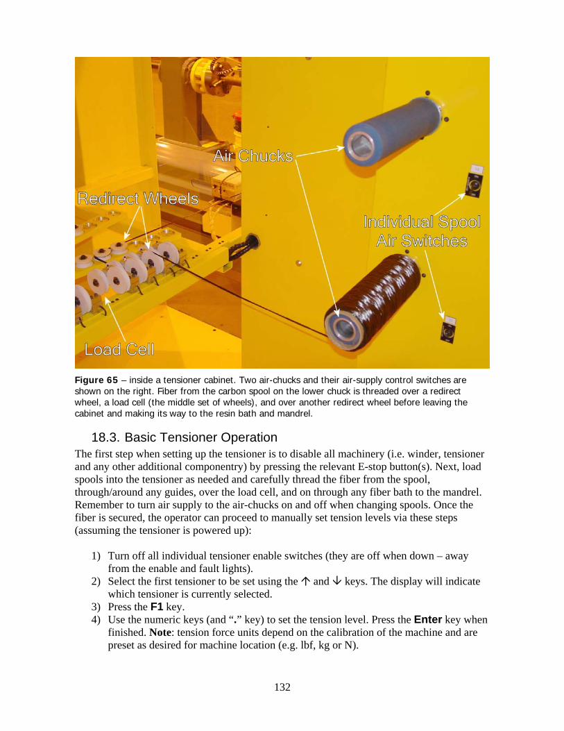
Figure 65 – inside a tensioner cabinet. Two air-chucks and their air-supply control switches are shown on the right. Fiber from the carbon spool on the lower chuck is threaded over a redirect wheel, a load cell (the middle set of wheels), and over another redirect wheel before leaving the cabinet and making its way to the resin bath and mandrel.

18.3. Basic Tensioner Operation The first step when setting up the tensioner is to disable all machinery (i.e. winder, tensioner and any other additional componentry) by pressing the relevant E-stop button(s). Next, load spools into the tensioner as needed and carefully thread the fiber from the spool, through/around any guides, over the load cell, and on through any fiber bath to the mandrel. Remember to turn air supply to the air-chucks on and off when changing spools. Once the fiber is secured, the operator can proceed to manually set tension levels via these steps (assuming the tensioner is powered up):

1) Turn off all individual tensioner enable switches (they are off when down – away from the enable and fault lights).

2) Select the first tensioner to be set using the and keys. The display will indicate which tensioner is currently selected.

3) Press the F1 key. 4) Use the numeric keys (and “.” key) to set the tension level. Press the Enter key when

finished. Note: tension force units depend on the calibration of the machine and are preset as desired for machine location (e.g. lbf, kg or N).

132

5) Repeat steps 2 – 4 for each tensioner to be used. 6) When all tensions are set, press the main enable button (the green button above the

red e-stop button). 7) Finally, turn on the individual tensioners enable switches of the tensioners which

were set in the previous steps. The operator should notice the tautness in the lines as each tensioner comes up.

Note: leaving the individual tensioners switches enabled and using the main enable switch to turn on all tensioners at once is not recommended. It generates more abrupt motion and has greater potential for operator error. Once the drives have been enabled, the operator may use the individual enable switches to remove tension from an individual tensioner. Cycling these switches on and off can also be used to clear a tensioner fault (but this method is not recommended when replacing a fiber spool or splicing a broken fiber).

Figure 66 – close-up of the tensioner keypad/display and individual tensioner enable switches across the top with their enable (green) and fault (red) lights. In the picture, all enable switches are off: down, away from the lights.

Pressing the E-stop button (see Figure 64) will remove power from all drives in an emergency. Note that the motors do not incorporate any brakes and will drift to a stop (assuming the mandrel has stopped). To recover, we suggest first disabling all individual tensioners, then pressing the main, green enable button, and finally enabling the individual tensioners.

133

Pressing F2 will cause the computer to start displaying the current tension of the currently selected tensioner/motor. The value will be displayed for 100 times, then it will automatically stop.

18.4. Advanced Tensioner Controls The final section of this chapter (18.7) is a table providing a detailed list of all the tensioner keypad commands. Before attempting any advanced operation, be sure to read all the notes in this section. In general:

- Be aware of the current cursor shift-state: flashing for upper (blue) keys or (no display) for lower (white) keys. In the table, each key is preceded by one of the above symbols to remind you. After the first command key, the machine will generally switch shift mode as appropriate to assist with entry.

- The table indicates the sequence of commands to enter to complete the given

procedure. The software may not always indicate an error input (e.g. if password entry fails, the software will display the string “<DONE>”). If the command prompts do not appear to follow the sequence, then the sequence has probably failed, generally due to an invalid input. To restart a sequence, try pressing ESC a few times and then press the or key which will display a message about the currently selected tensioner. Then restart the sequence.

- The software generally displays a confirmation message once a procedure has

completed. Password – all operations which permanently record data on the tensioner require entry of a password. The factory default password is: 1234 (number keys are shift insensitive). Be careful when changing the password. If the password is lost, contact McClean Anderson service for information on restoring it. Calibration – The load cells can be recalibrated to compensate for drift over time or to alter unit systems (see note below on unit systems). IMPORTANT NOTE: remove power to the drives by pressing the E-Stop button and turning off the tensioner enable switches (Figure 64) before calibrating! The tensioning system itself is essentially unitless – units are established based on the number the user enters to represent the force applied to the system. Note that “set tension” commands are based on this calibration setting – so if the system is calibrated in lbf, then commands issued via the tensioner control keypad or Omniwind would generate a tension in lbf). For example, assume the user applies a force corresponding to a 5lb weight along the fiber path. The following calibration entries correspond to different units of force:

5 – the system is calibrated in lbf 2.268 – the system would be calibrated in kgf (where 1kgf = 2.205lbf) 22.25 – the system would be calibrated in Newtons (where 9.81N = 1kgf)

134

Important Note: in the present generation of code, a calibration setting in lbf is strongly recommended due to internally applied limits to protect the load cell from tension overload. On standard, 10lbf tensioners, the range of allowable tension units is from 0 to 12 (the user should only set up to 10lbs, the additional margin is for dynamic response) – if the device sustains tension above 12units, it will error out and disable the unit (and put the winder in Hold). Calibration in kgf would allow an overload condition and prevent the safety measure from engaging. This is because the safety feature doesn’t apply until 12kg, which is beyond the load cell’s range – it will saturate before reaching 12 units so the machine will never fault out. A setting in Newtons would not allow full use of the available tension range, causing a fault once the device reaches 12N (and also preventing the user from entering larger values). This should be remedied in a later firmware release which will incorporate additional unit information. To calibrate the tensioner, the first step is to obtain a means of generating a calibrating force. This can simply be a known weight. To improve accuracy, select a weight at the upper end of the tensioner’s range (10lb. for standard machines). Begin at the spool end: fix the fiber by tying it around the spool. Then thread the fiber through the tensioner rollers and load cell as it would be routed during operation (it is important that the fiber enter and exit the roller on the load-cell in the same manner as during operation because this will affect the measured value). Finally, redirect the fiber path so that it becomes vertical. Depending on the layout of the tensioning system, this might be possible by using rollers which are already part of the system – such as rollers on other tensioners. The path should be kept as low-friction as possible (e.g. use low-friction rollers, not a rounded bar to redirect the fiber path) to improve calibration accuracy. Finally, affix the known weight to the end of the fiber. Note that the procedure requires two readings – an unloaded and a loaded cell. The software provides sufficient time and keystroke sequences for a single operator to load and unload the cell at the appropriate times, although the procedure is easier with two operators. The individual command sequences are covered in the table (see section 18.7). Command F5 initiates the calibration sequence. During the sequence, the operator is instructed to unload the tensioner (remove the weight). The device will then take measurements and produce a D0[#] calibration value (where # is the number of the tensioner being calibrated). The operator is then instructed to load the tensioner (apply the weight) and another series of measurements is carried out. This time the tensioner will display two additional calibration values D1[#] and C[#]. The operator may record D0[#] and C[#] for later manual entry if desired. The new calibration values are put to immediate use once the machine is enabled (of course this requires the operator to first remove the calibration equipment and rethread fiber for normal use). These values are lost when the machine is shut down, which is useful if the operator is concerned about their validity. To make the new calibration values permanent, a save calibration command sequence is executed (K command), which records current calibration settings on all tensioner units. The user can also enter previously recorded calibration values manually using the E command (these would also need to be saved to make them permanent).

135

Kp and Ki gain adjustment – The user can alter the gains to fine-tune the performance of the tensioner. The proportional (Kp) and integral (Ki) controller gains are available. These gains may be increased by trial and error to achieve a faster response. One approach is to start with Kp and Ki set to zero. Then bring Kp up to achieve reasonable motion performance, and finally increase Ki gradually (order of 0.01) until a satisfactory response is obtained. Performance can be checked by doing an actual test wind. If either gain is set too high, the system may become unstable and oscillate. Pressing F3 will display the current values of Kp and Ki for each tensioner. These can be used as a reference for tuning. Ki will affect the tension ramp-up time and Kp will affect the instantaneous response of the tensioner. When increasing Ki to reduce the tension ramp-up time, consider decreasing Kp first to avoid an unstable condition. As a rule, tuning a control system requires patience and experience. Sometimes, when the range of tension values, fiber type, or type of winding programs change, the controller gains may require adjustment as well. Tensioner fault levels – the tensioner software uses two methods to detect fiber breakage and throw a fault:

- The first is a low-tension threshold. That means if the tension feedback from the sensor stays below the set threshold value for longer than the adjustable time-out interval, then it will error out. Note: this value is entered in seconds, but when the operator saves the fault threshold settings, the software will display the time-out interval in terms of sample counts. For example, if the sampling frequency is set to 1,000 Hz then a value of 500 would correspond to 0.5seconds. So once the computer sees load-cell values below the threshold for more than 0.5 seconds, the given tensioner would fault-out.

- The second method is the tension-drop criteria. This performs a sample-by-sample evaluation of the load-cell checking for major, near-instantaneous changes in the load, likely to signal a disruption in the fiber. This is set via a fixed factor. For example, if the factor were 0.8, then if any sample were less than 80% of its predecessor, the tensioner would fault-out. In practice, the low-frequency mechanical characteristics of the system tend to limit the practicality of this method.

Increasing the low-tension threshold level, decreasing the time-out interval value, and increasing the tension-drop factor all work towards faster and more frequent tensioner faults. Decreasing the time-out interval value by itself can speed up how quickly the tensioner is able to detect a break which can be quite valuable at limiting the amount of fiber take-up and subsequent rethreading/clean-up.

18.5. Automated Operation with Omniwind Connecting a tensioning system to an Omniwind control greatly enhances its capabilities. Omniwind is able to both directly control tension settings on the tensioners, and to also gather telemetry data from the tensioners and record these to a log file. Furthermore, tension levels can also be directly incorporated into wind programs through use of Coordinator

136

software. For more information on these topics see section 17.10 on Omniwind and chapter 20 on Coordinator. One important note: the tensioning control system is non-hierarchical – requests are executed in sequence. For example, if a particular wind program sets tension levels on a repeating basis and the operator manually sets different levels at the tensioner, those manual levels will be used until the next time the wind-program triggers the condition and generates a new request. When using wind-program based control (via Coordinator), the Omniwind dialog box control (Figure 62) is disabled for any unit which is controlled in the wind program. Control is always available via the tensioning computer/keypad.

18.6. Troubleshooting Problem: The tensioner computer locks up. Solution: This may be caused by corrupted control file settings (e.g. a zero for an error out interval which generates a divide by zero exception). Contact McClean Anderson to resolve this problem. Problem: Violent motion Solution: This may be caused by incorrect calibration settings which causes the tensioner to misinterpret the sensor’s feed back signals. Another possibility is that the Kp and Ki gain values are either too high or the files containing these values have become corrupted. Try to recalibrate the tensioner(s) in question and/or adjust the gains. If these steps fail, please contact McClean Anderson service. Problem: Slow ramp-up speed to new tension setting Solution: This may indicate that Ki is too small. Try decreasing Kp first and then increasing Ki gradually.

Problem: Tensioner faults-out, a red light appears above its enable switch, Omniwind behaves erratically Solution: in general, this is a fairly normal occurrence due to the fiber spool running out. In such a case, a new spool must be loaded (see instructions for this in section 18.3). Note that in most tensioning systems, the fault condition is linked to Omniwind’s Hold pushbutton so that when a fault occurs, the machine automatically stops. If the operator is unaware of this, this can cause some confusion because Omniwind will no longer wind but many other functions will continue to work. If the fault is not caused by the end-of-spool condition, this may be a sign that the fiber break sensing algorithms have overly sensitive settings. First, manually remove any slack in the problem tow by rewinding the spool / motor (remembering the safety guidelines about first putting the tensioner in EStop). Then restart the system & problem tow. If this is successful, try to proceed with the wind at gradually higher speeds. If the problem resurfaces, consider adjusting the tensioner fault levels and/or increasing the controller gains to improve performance (see section 18.4 for more details on both). Problem: Fiber has excessive vibration

137

Solution: In some cases, a particular wind and machine orientation may generate high fiber acceleration rates which are challenging to track. As a first step, the operator may simply try a higher tension. If that is unacceptable or does not improve the situation, the system may require higher gain settings. See section 18.4 for more details.

138

18.7. Tensioner Command Table Remember and indicate shift key state ( for upper, “blue” keys, - no display - for lower, “white” keys)

Key Function Steps Notes Change current tensioner Press Up arrow key Lowers current tensioner number, stops at the first tensioner

Change current tensioner Press Down arrow key Increases current tensioner number, stops at the last tensioner F1 Set tension 1. Select motor (via , )

2. Press F1 3. Input tension value

Select motor via , before pressing F1. See commands above and section 18.3.

F2 Display measured tension value

Press F2 The value will be displayed for 100 times in the format: “Motor #: Tension”

F3 Display gains Kp and Ki for each tensioner

1. Press F3 2. Press Enter to display values for each tensioner in sequence

F4 Set gains Kp and Ki for one tensioner

1. Press Y to confirm 2. Input tensioner number 3. Input Kp 4. Input Ki 5. Press Y to make setting global – see *

Any input error will cancel the operation. New values take effect but are not saved to a file (see instructions for D below). * - When finished, if all individual tensioners are currently disabled, computer will ask if new gains should apply to all tensioners - enter Y if this is desired.

F5 Do load-cell calibration for one tensioner

1. Turn off all tensioners 2. Press F5 3. Press Y to confirm 4. Press Y again after prompt 5. Input tensioner number 6. Remove any load from the tensioner 7. Press S 8. Record D0[#] value for future reference if desired (# is tensioner number) 9. Press any key 10. Apply a known force to the load-cell (e.g. hanging a weight or pulling fiber with a precision tension gauge) 11. Input known tension applied to be calibrated 12. Press S 13. Record C value for future reference if desired 14. Press any key to complete sequence

Keep all tensioners off during calibration sequence. D0[#] and C are calibration values. Record these for future reference if desired. During calibration the computer will sample the load cell 500 times for the zero and the maximum force settings and average the results. The data will take affect immediately, but will not be stored unless a save command is executed (see instructions for K). If you feel the calibration is incorrect, turn off the power for 5 minutes and then back on. The control will revert to the last saved values. To manually enter the load cell calibration values (D0[#] & C), see instructions for E.

139

Key Function Steps Notes A Change Password 1. Press A

2. Press Y to confirm 3. Type in current password 4. Type in new password 5. Press Y to confirm and save password

Passwords are always 4 characters. New password is permanently saved (i.e. no separate save sequence necessary).

B Change basic control settings for tensioner

1. Press B 2. Press Y to confirm 3. Input password 4. Input sampling frequency 5. Input tension ramping up time 6. Input delay value for telemetry display 7. Press Y to save changes to file

Max sampling frequency is 1.5 KHz. We recommend 1KHz. This value does not need to be changed. If all inputs are valid, then the new settings will be saved to a file immediately. Tension ramping time is used to pull the fiber tight at startup. Recommended value is 12 seconds. Telemetry delay value determines how quickly F2 command displays load-cell readings. A value of 5000 is recommended. The larger the count, the longer the delay between measurement updates.

L Change error thresholds for Fiber breakage

1. Press L 2. Press Y to confirm 3. Input tensioner number 4. Input time-out interval (in seconds) 5. Input low tension error threshold (% of set tension) 6. Press Y to make setting global – see *

These values are used to check for tensioner faults (e.g. fiber breakage). If tension levels drop to less than the entered fraction of target settings for longer than the time-out interval, the tensioner will fault. * - When finished, if all individual tensioners are currently disabled, computer will ask if values should apply to all tensioners - enter Y if this is desired.

M Save error thresholds for all tensioners

1. Press M 2. Press Y to confirm 3. Input password 4. Press Enter to display values for each tensioner in sequence 5. Press Y to save the values to file

The computer allows the user to verify each time-out delay and error threshold value before committing them. When displaying the time-out delay, the value is shown in sample intervals (i.e. 1000 = 1second at typical sampling frequency of 1kHz).

D Save gain values for all tensioners

1. Press D 2. Press Y to confirm 3. Input password 4. Press Enter to display values for each tensioner in sequence 5. Press Y to save the values to file

The computer allows the user to verify each Kp (proportional) and Ki (integral) gain value before committing (or discarding) them.

E Input calibration data for one tensioner

1. Press E 2. Input tensioner number 3. Input D0[#] value recorded for this tensioner 4. Input C value recorded for this tensioner

See instructions on F5 above for information on calibrating the load-cells and generating appropriate calibration data. New values take effect immediately but are not saved to a file (see instructions for K).

140

Key Function Steps Notes K Save calibration data for

all tensioners 1. Press K 2. Press Y to confirm 3. Enter password 4. Press Enter to scroll through calibration data 5. Press Y to save the values to file

The computer allows the user to verify calibration values for each tensioner load cell before committing (or discarding) them. A confirmation message is displayed upon sequence completion.

U Set tension for all tensioners at once

1. Press U (for Universal) 2. Input tension value for all tensioners

( Input sample interval tension drop for fiber breakage detection

1. Press ( 2. Press Y to confirm 3. Input tensioner number 4. Input tension drop percentage threshold (Pdrop) 5. Press Y to make setting global – see *

Pdrop is evaluated against the current sampled tension value divided by the previous sampled tension value and must be set between 0 and 1. So 0.5 will trigger a fault if the measured tension drops by 50% between two samples. * - When finished, if all individual tensioners are currently disabled, computer will ask if values should apply to all tensioners - enter Y if this is desired.

) Save Pdrop variables for all tensioners

1. Press ) 2. Press Y to confirm 3. Enter password 4. Press Enter to display values for each tensioner in sequence 5. Press Y to save the values to file

The computer allows the user to verify Pdrop values for each tensioner before committing (or discarding) them.

N Input start-up, fault evaluation delay value

1. Press N 2. Press Y to confirm 3. Input tensioner number 4. Input delay value (seconds) 5. Press Y to make setting global – see *

This timeout value applies when the tensioner is turned ON at the toggle switch. The low-tension fault check (see commands L and M) is not carried out over this initial delay to allow the tensioners to remove any slack in the system. * - When finished, if all individual tensioners are currently disabled, computer will ask if values should apply to all tensioners - enter Y if this is desired.

O Save the error checking delay times

1. Press O 2. Press Y to confirm 3. Enter password 2. Press Enter to display values for each tensioner in sequence 3. Press Y to save the values to file

The computer allows the user to verify Pdrop values for each tensioner before committing (or discarding) them.

, Toggle Backlight of LCD Press “,” (comma key) Does not apply to VFD-type displays (Vacuum Fluorescent Display – these have a bright, greenish-blue readout).

141

A. Verifying Part Coverage and Pattern Closure This appendix gives a brief mathematical overview on how to verify that a particular program covers the mandrel and generates a closed pattern. In general, the winding software takes care of these issues automatically. However, advanced users who directly edit the motion table may use this as a reference when creating specialized winds. For purposes of this manual, full part coverage implies a mandrel will be fully covered in fiber, assuming that its pattern also closes. A closed pattern implies that the fiber is evenly distributed around the mandrel (e.g. there are no filled in areas with large gaps between them). Note that in reality, full coverage actually implies two layers of fiber at each location – one running at the positive fiber angle and the other running at the negative one. A quick estimate of the critical angle for coverage is the arccosine of the fiber bandwidth multiplied by the number of circuits and divided by the circumference of the part.

For example, a 6 inch diameter part with a 1 inch bandwidth and 7 circuits for coverage would yield 1 inch times 7 circuits divided by six and then divided by pi resulting in 0.37136. The arccosine of this is 68.2 degrees – angles higher than this would begin to overlap, lower angles would gap.

When using the software to generate a part, the process is somewhat reversed – the user specifies diameter, bandwidth, and angle and the software establishes how many circuits are required (note: the solution winds will have two different number of circuits – one rounding up and one rounding down). A similar method is useful for estimating wind angles for constant coverage on non-linear winds. In this case, given some initial target angle (t) at a particular radius (r1), the appropriate angle (b) at a different radius (r2) would be determined by taking the ratio of r1 over r2, dividing this by the cosine of t, and taking the arccosine of the result. If this is impossible (trying to take an arc-cosine of a value greater than 1), the resulting angle is zero and there will still be overlap. Note that in practical terms this is useful for parts with a limited change in diameter – for very large differences, the resulting angles tend to vary to such a degree that the resulting structural changes and fiber instability make this attempt at constant coverage everywhere of limited use. Also note that obtaining constant coverage runs counter to the goal of obtaining a stable fiber path (for constant coverage, as the diameter grows, the fiber angle increases, while for a stable path, as the diameter grows the fiber angle decreases). To determine if a particular wind closes, the first step is to sum the angle column for a circuit. The SUM() spreadsheet function works well for this (remember that the first delta mandrel line of any particular segment belongs to the previous segment). The resulting number should then be multiplied by the number of circuits. This should yield a whole number which is divisible by 360 (the first test). This number should then be divided by 360 and then by the number of circuits. We are interested in the remainder (or modulus) of this second division. To obtain the remainder, drop the whole number portion and multiply the

151

fraction by the number of circuits. We now need to compare this remainder with the number of circuits. If these numbers have a common divisor (i.e. they both can be evenly divided by the same number other than one), then the pattern will not properly close, otherwise it will. If the remainder is zero, the pattern will also fail to close. The resulting wind pattern can be determined by the modulus and the number of circuits. Unfortunately, a detailed description of how to obtain the pattern type from this data is beyond the scope of this manual. As an example:

A particular wind requires 789.6774292 degrees per circuit. The wind also requires 31 circuits to complete. So, the first step is to multiply 789.677 by 31 giving 24480. Dividing by 360 gives 68 (evenly). 68 divided by 31 is 2.193548387. Subtracting 2 and then multiplying by 31 gives a modulus of 6, so our two numbers are 6 and 31. The divisors of 6 are 2 and 3 while 31 in a prime number. Since there are no common divisors, this wind pattern closes. The pattern would generally be described as a 5 lead pattern (after 5 circuits, the mandrel is located at 5*6/31, or 30/31, of a revolution from its start, or one bandwidth before – leading – the initial band).

As an example of failure and correction:

A particular segment has 895 degrees of mandrel rotation and a target of 24 circuits to complete the pattern. The first step is to multiply 895 by 24 giving 21480. This is not divisible by 360 – the division result would be 59.6667.

The first correction is to add (or subtract) enough motion per circuit to attain a pattern divisible by 360. If we take the division result and increase (or decrease) it to the next whole number, and multiply this by 360, we obtain a target angle for the complete segment. Dividing this by the number of circuits gives us the target rotation per circuit – the original motion needs to be adjusted to this value. This could be obtained via scaling, direct insertion of motion, etc.

In the example, we would try for 60 rotations or 21600 degrees. Dividing this by 24 gives 900 degrees per circuit, or an additional 5 degrees of motion required. Continuing with the evaluation, our complete wind is 21600. Dividing by 360 gives 60 rotations. 60 divided by 24 is 2.5. Subtracting the 2 and multiplying by 24 yields 12. Our critical numbers are 12 and 24. These obviously have many common divisors (2, 3, 4, 6, and 12) so our wind pattern would not complete (after 2 circuits, the pattern would overlap itself – we would move the mandrel 1800 degrees and be back at the starting point). Again, we need to increase (or decrease) the wind by enough degrees to properly close.

To increase (or decrease) a wind by an appropriate amount, the increment (decrement) is 360 divided by the number of circuits.

152

In the example, the increment would be 360 divided by 24 or 15 degrees. We could try for 885 or 915 degrees. Using 885 (closer to the starting value), we would obtain a total mandrel motion of 885 times 24 or 21240. Divided by 360 yields 59. 59 divided by 24 yields 2.458333. Subtracting 2 then multiplying by 24 yields 11. 11 and 24 have no common divisors (had we added 15 degrees per circuit, the result would have been 24 and 13 – which also closes – the increment/decrement generally solves the problem). The resulting part would have an 11-lag pattern.

These are the types of calculations done automatically in Composite Designer. However, if the user is experimenting with sophisticated, direct editing of machine motion, then they need to be aware of these concepts to assist with appropriate motion generation.

153