Evaluationoftheseismicperformanceofacode-conforming reinforced …bechtel.colorado.edu/~porterka/Goulet-et-al-2007-PEER... · · 2008-10-17Evaluationoftheseismicperformanceofacode-conforming

EARTHQUAKE ENGINEERING AND STRUCTURAL DYNAMICSEarthquake Engng Struct. Dyn. 2007; 36:1973–1997Published online 15 June 2007 in Wiley InterScience (www.interscience.wiley.com). DOI: 10.1002/eqe.694

Evaluation of the seismic performance of a code-conformingreinforced-concrete frame building—from seismic hazard to

collapse safety and economic losses

Christine A. Goulet1,∗,†, Curt B. Haselton2, Judith Mitrani-Reiser3, James L. Beck3,Gregory G. Deierlein2, Keith A. Porter3 and Jonathan P. Stewart1

1Department of Civil and Environmental Engineering, UCLA, Los Angeles, CA 90095, U.S.A.2Department of Civil and Environmental Engineering, Stanford University, Stanford, CA 94305, U.S.A.

3Division of Engineering and Applied Science, Caltech, Pasadena, CA 91125, U.S.A.

SUMMARY

A state-of-the-art seismic performance assessment is illustrated through application to a reinforced-concrete moment-frame building designed per current (2003) building code provisions. Performance isquantified in terms of economic losses and collapse safety. The assessment includes site-specific seismichazard analyses, nonlinear dynamic structural response simulations to collapse, damage analyses, and lossestimation. When selecting ground motion records for nonlinear dynamic analyses that are consistent witha target hazard level expressed in terms of a response spectral value at the building’s fundamental period, itis important to consider the response spectral shape, especially when considering higher hazard levels. Thiswas done through the parameter commonly denoted by �. Neglecting these effects during record selectionis shown to lead to a factor of 5–10 overestimation of mean annual collapse rate. Structural responsesimulations, which properly account for uncertainties in ground motions and structural modelling, indicatea 2–7% probability of collapse for buildings subjected to motions scaled to a hazard level equivalentto a 2% probability of exceedance in 50 years. The probabilities of component damage and the meansand coefficients of variation of the repair costs are calculated using fragility functions and repair-costprobability distributions. The calculated expected annual losses for various building design variants rangefrom 0.6 to 1.1% of the replacement value, where the smaller losses are for above-code design variants andthe larger losses are for buildings designed with minimum-code compliance. Sensitivity studies highlightthe impact of key modelling assumptions on the accurate calculation of damage and the associated repaircosts. Copyright q 2007 John Wiley & Sons, Ltd.

Received 31 August 2006; Revised 31 January 2007; Accepted 22 March 2007

KEY WORDS: seismic; performance; assessment; building; epsilon; collapse; losses

∗Correspondence to: Christine A. Goulet, Department of Civil and Environmental Engineering, UCLA, Los Angeles,CA 90095, U.S.A.

†E-mail: [email protected]

Contract/grant sponsor: Earthquake Engineering Research Centers Program of the National Science Foundation;contract/grant number: EEC-9701568Contract/grant sponsor: National Sciences and Engineering Research Council of CanadaContract/grant sponsor: le Fonds quebecois de la recherche sur la nature et les technologies

Copyright q 2007 John Wiley & Sons, Ltd.

1974 C. A. GOULET ET AL.

1. INTRODUCTION

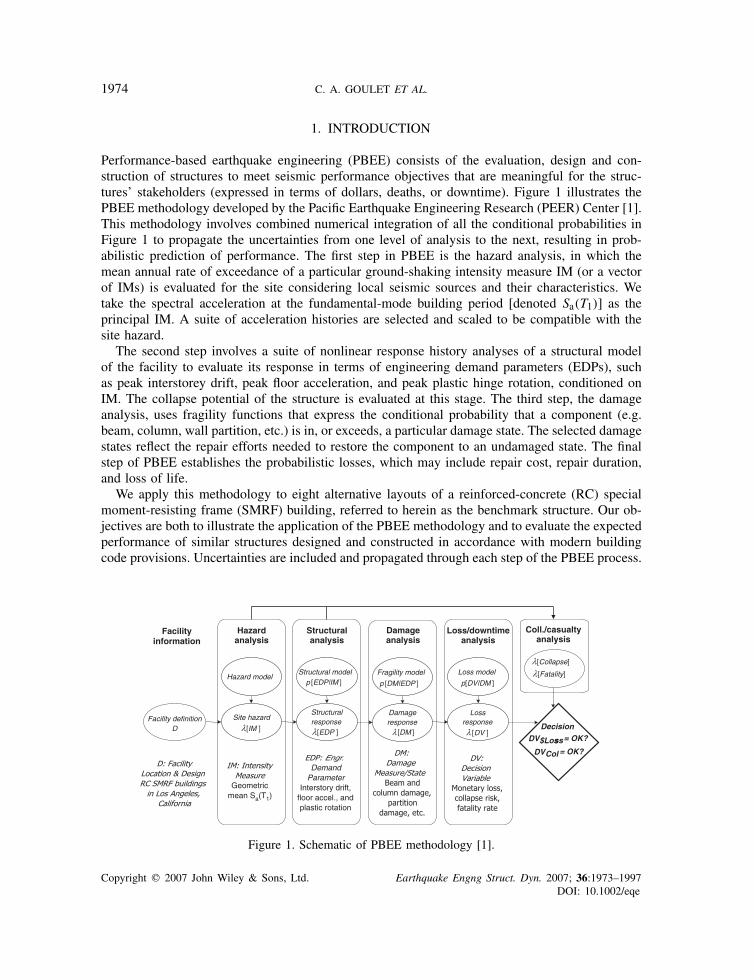
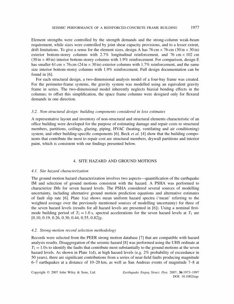
Performance-based earthquake engineering (PBEE) consists of the evaluation, design and con-struction of structures to meet seismic performance objectives that are meaningful for the struc-tures’ stakeholders (expressed in terms of dollars, deaths, or downtime). Figure 1 illustrates thePBEE methodology developed by the Pacific Earthquake Engineering Research (PEER) Center [1].This methodology involves combined numerical integration of all the conditional probabilities inFigure 1 to propagate the uncertainties from one level of analysis to the next, resulting in prob-abilistic prediction of performance. The first step in PBEE is the hazard analysis, in which themean annual rate of exceedance of a particular ground-shaking intensity measure IM (or a vectorof IMs) is evaluated for the site considering local seismic sources and their characteristics. Wetake the spectral acceleration at the fundamental-mode building period [denoted Sa(T1)] as theprincipal IM. A suite of acceleration histories are selected and scaled to be compatible with thesite hazard.

The second step involves a suite of nonlinear response history analyses of a structural modelof the facility to evaluate its response in terms of engineering demand parameters (EDPs), suchas peak interstorey drift, peak floor acceleration, and peak plastic hinge rotation, conditioned onIM. The collapse potential of the structure is evaluated at this stage. The third step, the damageanalysis, uses fragility functions that express the conditional probability that a component (e.g.beam, column, wall partition, etc.) is in, or exceeds, a particular damage state. The selected damagestates reflect the repair efforts needed to restore the component to an undamaged state. The finalstep of PBEE establishes the probabilistic losses, which may include repair cost, repair duration,and loss of life.

We apply this methodology to eight alternative layouts of a reinforced-concrete (RC) specialmoment-resisting frame (SMRF) building, referred to herein as the benchmark structure. Our ob-jectives are both to illustrate the application of the PBEE methodology and to evaluate the expectedperformance of similar structures designed and constructed in accordance with modern buildingcode provisions. Uncertainties are included and propagated through each step of the PBEE process.

Hazard model

Site hazard

[IM ]

IM: Intensity

Measure

Geometricmean Sa(T1)

Hazardanalysis

Facility definitionD

Structuralanalysis

Structural modelp [EDP|IM ]

Structuralresponse

[EDP ]

Damageanalysis

Fragility model

p [DM|EDP ]

Damageresponse

Loss/downtimeanalysis

Loss model

p[DV|DM ]

Lossresponse

[DV ]

Coll./casualtyanalysis

[Collapse]

EDP: Engr.Demand

ParameterInterstory drift,

floor accel., andplastic rotation

DM:

Damage

Measure/State

Beam and

column damage,

partition

damage, etc.

DV:

Decision

Variable

Monetary loss,

collapse risk,

fatality rate

Decision

DV$Losss= OK?

DVCol = OK?

D: Facility

Location & Design

RC SMRF buildings

in Los Angeles,

California

Facilityinformation

[Fatality]

[DM ]

Figure 1. Schematic of PBEE methodology [1].

Copyright q 2007 John Wiley & Sons, Ltd. Earthquake Engng Struct. Dyn. 2007; 36:1973–1997DOI: 10.1002/eqe

SEISMIC PERFORMANCE OF A REINFORCED-CONCRETE FRAME BUILDING 1975

Uncertainty in the factors affecting ground motions is accounted for through probabilistic seismichazard analysis (PSHA). EDP distributions evaluated from the structural response simulationsreflect record-to-record variability, that is, the uncertainty remaining only when the shaking intensityis known. Structural modelling uncertainties are not included in the damage and repair-cost analysesfor the non-collapse cases, but they are included for collapse predictions, where they are shownto have a significant effect. The damage and loss analyses treat all the uncertainties in DM givenEDP, and DV given DM.

2. SITE SELECTION AND DESCRIPTION

The benchmark structure is located on deep sediment near the centre of the Los Angeles basin,at 33.996◦N, 118.162◦W, south of downtown Los Angeles. The site is within 20 km of sevenknown faults, but no single major fault produces near-fault motions that dominate the site hazard.High-quality geotechnical data are available for this site from the ROSRINE program [2] accordingto which the upper 30m consist of sands and silts with traces of clay and cobbles with an averageshear wave velocity Vs−30 = 285 m/s (NEHRP soil category D).

3. BENCHMARK BUILDING DESIGN

3.1. Structural design

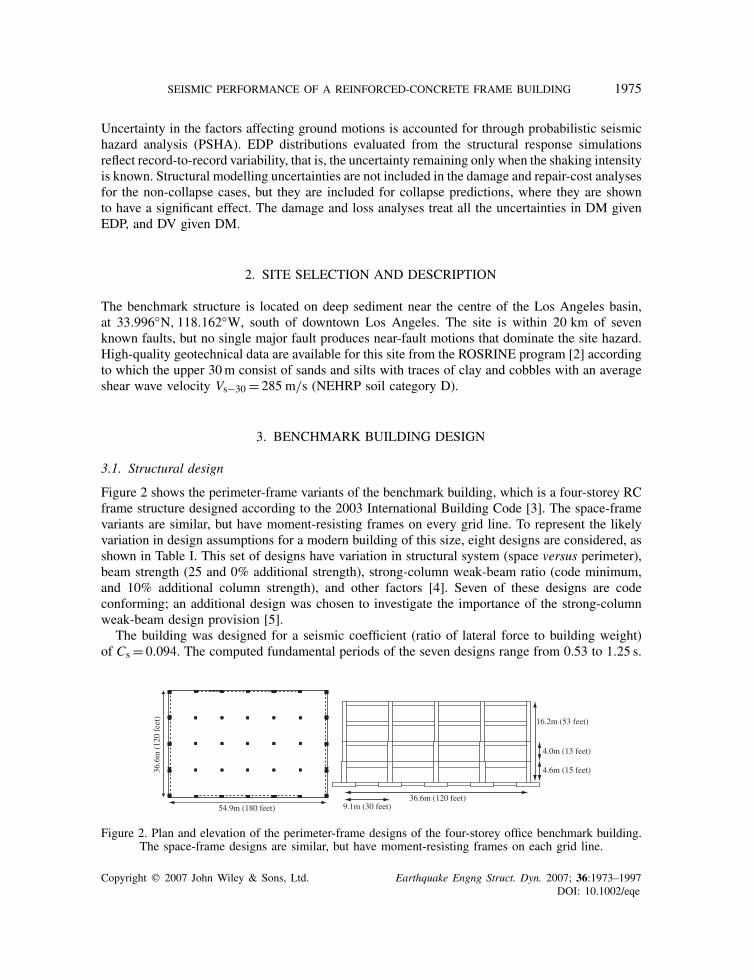
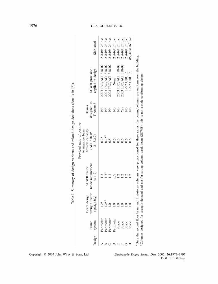
Figure 2 shows the perimeter-frame variants of the benchmark building, which is a four-storey RCframe structure designed according to the 2003 International Building Code [3]. The space-framevariants are similar, but have moment-resisting frames on every grid line. To represent the likelyvariation in design assumptions for a modern building of this size, eight designs are considered, asshown in Table I. This set of designs have variation in structural system (space versus perimeter),beam strength (25 and 0% additional strength), strong-column weak-beam ratio (code minimum,and 10% additional column strength), and other factors [4]. Seven of these designs are codeconforming; an additional design was chosen to investigate the importance of the strong-columnweak-beam design provision [5].

The building was designed for a seismic coefficient (ratio of lateral force to building weight)of Cs = 0.094. The computed fundamental periods of the seven designs range from 0.53 to 1.25 s.

54.9m (180 feet)

36.6

m (

120

feet

)

36.6m (120 feet)9.1m (30 feet)

4.6m (15 feet)

4.0m (13 feet)

16.2m (53 feet)

Figure 2. Plan and elevation of the perimeter-frame designs of the four-storey office benchmark building.The space-frame designs are similar, but have moment-resisting frames on each grid line.



TableI.Su

mmaryof

design

variants

andrelateddesign

decisions(details

in[6]

).

Provided

ratio

ofpo

sitiv

eto

negativ

ebeam

Beam

design

SCWB

factor

flexu

ralcapacity

Beams

Fram

estreng

thfactor

(cod

erequ

irem

ent

(ACI31

8-05

design

edas

SCWB

provision

Design

system

( �Mn/Mu)

is1.2)

21.3.2.2)

T-beam

s?appliedin

design

Slab

steel

APerimeter

1.25

1.3

0.75

No

2003

IBC

/ACI31

8-02

2#4@

12′′o.c.

BPerimeter

1.25

∗1.3∗

0.75

∗No

2003

IBC

/ACI31

8-02

2#4@

12′′o.c.

CPerimeter

1.0

1.2

0.5

No

2003

IBC

/ACI31

8-02

2#4@

12′′o.c.

DPerimeter

1.0

n/a

0.5

No

Non

e†2#4@

12′′o.c.

ESp

ace

1.0

1.2

0.5

No

2003

IBC

/ACI31

8-02

2#4@

12′′o.c.

FSp

ace

1.0

1.2

0.5

Yes

2003

IBC

/ACI31

8-02

2#4@

12′′o.c.

GSp

ace

1.0

1.2

0.5

No

1997

UBC

[5]2#4@

12′′o.c.

HSp

ace

1.0

1.2

0.5

No

1997

UBC

[5]#5,#6@

16′′o.c.

∗ Onlythesecond

floor

beam

andfirst-storeycolumns

wereprop

ortio

nedfortheseratio

s;thebeam

s/columns

areun

iform

over

thebuild

ing.

† Colum

nsdesign

edforstreng

thdemandandno

tforstrong

-colum

nweak-beam

(SCWB);this

isno

tacode-con

form

ingdesign

.



Element strengths were controlled by the strength demands and the strong-column weak-beamrequirement, while sizes were controlled by joint shear capacity provisions, and to a lesser extent,drift limitations. To give a sense for the element sizes, design A has 76 cm× 76 cm (30 in× 30 in)exterior bottom-storey columns with 2.7% longitudinal reinforcement, and 76 cm× 102 cm(30 in× 40 in) interior bottom-storey columns with 1.9% reinforcement. For comparison, design Ehas smaller 61cm× 76cm (24 in× 30 in) exterior columns with 1.7% reinforcement, and the samesize interior bottom-storey columns with 1.9% reinforcement. Full design documentation can befound in [6].

For each structural design, a two-dimensional analysis model of a four-bay frame was created.For the perimeter-frame systems, the gravity system was modelled using an equivalent gravityframe in series. The two-dimensional model inherently neglects biaxial bending effects in thecolumns; to offset this simplification, the space frame columns were designed only for flexuraldemands in one direction.

3.2. Non-structural design: building components considered in loss estimates

A representative layout and inventory of non-structural and structural elements characteristic of anoffice building were developed for the purpose of estimating damage and repair costs to structuralmembers, partitions, ceilings, glazing, piping, HVAC (heating, ventilating and air conditioning)system, and other building-specific components [6]. Beck et al. [4] show that the building compo-nents that contribute the most to repair cost are structural members, drywall partitions and interiorpaint, which is consistent with our findings presented below.

4. SITE HAZARD AND GROUND MOTIONS

4.1. Site hazard characterization

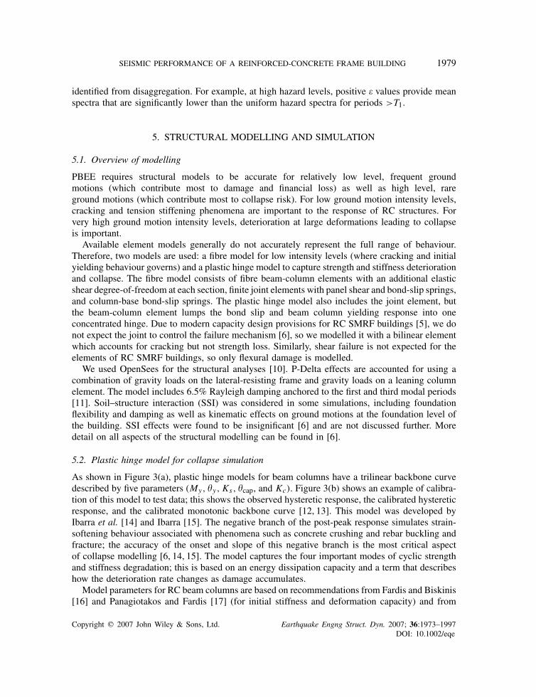
The ground motion hazard characterization involves two aspects—quantification of the earthquakeIM and selection of ground motions consistent with the hazard. A PSHA was performed tocharacterize IMs for seven hazard levels. The PSHA considered several sources of modellinguncertainty, including alternative ground motion prediction equations and alternative estimatesof fault slip rate [6]. Plate 1(a) shows mean uniform hazard spectra (‘mean’ referring to theweighted average over the previously mentioned sources of modelling uncertainty) for three ofthe seven hazard levels (results for all hazard levels are presented in [6]). Using a nominal first-mode building period of T1 = 1.0 s, spectral accelerations for the seven hazard levels at T1 are[0.10, 0.19, 0.26, 0.30, 0.44, 0.55, 0.82]g.

4.2. Strong-motion record selection methodology

Records were selected from the PEER strong motion database [7] that are compatible with hazardanalysis results. Disaggregation of the seismic hazard [8] was performed using the UHS ordinate atT1 = 1.0s to identify the faults that contribute most substantially to the ground motions at the sevenhazard levels. As shown in Plate 1(d), at high hazard levels (e.g. 2% probability of exceedance in50 years), there are significant contributions from a series of near-field faults producing magnitude6–7 earthquakes at a distance of 10–20 km, as well as San Andreas events of magnitude 7–8 at



distance 50–60km. At lower hazard levels, many magnitude and distance bins contribute similarlyto the estimated ground motion (Plate 1(b) and (c)).

In addition to magnitude and distance, the disaggregation was performed on � (‘epsilon’),which is a period-dependent quantity that measures the normalized offset of spectral accelera-tion at a given period [(Sa)] from the median that is expected from ground motion predictionequations

�= ln(Sa) − �Sa

�Sa(1)

where �Sa and �Sa are predicted values of the median and standard deviation (in lognormal units)of Sa from these predictions. Baker and Cornell [9] have shown that � is a predictor of spectralshape that can significantly affect nonlinear structural response among ground motion records withthe same Sa(T1) value. These dependencies occur because � correlates with spectral shape, withhigh positive �(T1) correlating with a peak in the acceleration spectrum at T1. When scaling theground motions to a target Sa(T1) value, an earthquake that has a peak in the acceleration spectrumat T1 is less damaging to a ductile building because of the reduction of spectral acceleration thatoccurs as period elongates past the peak.

At high hazard levels (Plate 1(d)), the disaggregation results reveal large positive epsilon values(�>1) for both the near-field, low-magnitude events and the far-field San Andreas events. Thisoccurs because the return period of the earthquakes on those sources is much lower than thereturn period of the ground motion. Hence, large � (i.e. a rare ground motion realization) is neededto produce the large ground motion associated with these high hazard levels. For relatively lowhazard levels (Plate 1(b)), nearby sources with higher magnitudes are characterized by relativelylow, often negative, � values. This occurs because large magnitude earthquakes on nearby faultsare likely to exceed a low ground motion level (i.e. the median from these sources exceeds theground motion level), thus producing negative �.

While the disaggregation results in Plate 1 strictly apply for a spectral period of 1s, very similarresults are obtained for the range of first-mode periods for the benchmark building design variants(with periods between 0.53 and 1.25 s). For example, at the 10% in 50 years hazard level, themean � values go from 1.2, 1.3 and 1.4 for the 0.5, 1 and 1.25 s periods, respectively, whereas themagnitude–distance distributions are negligibly affected. These variations are sufficiently smallthat they do not affect record selection.

For each of the seven hazard levels, independent suites of acceleration histories were selectedto represent the site hazard. The records populating each of these seven suites were selected to beconsistent with several aspects of the site hazard. First, records were sought that were compatiblewith the magnitude, distance, and epsilon disaggregation. All selected records were from deepsoil sites. For sources at close distance (<35 km), records with appropriate rupture directivityconditions were selected to be consistent with disaggregation results (details in [6]). Records wereselected based on the geometric mean of the two horizontal components, which is consistent withthe ground motion prediction equations used in PSHA. Accordingly, each record pair provides twohorizontal acceleration histories for use in structural simulations. All the selected records withina suite for a given hazard level were scaled such that their geometric mean matched the hazard-specific target {Sa(T1)}target. The average spectra of the selected records after scaling is shown inPlate 1(a) along with the uniform hazard spectra. For a given hazard level, the two spectra matchat T1 = 1.0 s, but deviate at other periods due to the spectral shape inherent to the scenario event



identified from disaggregation. For example, at high hazard levels, positive � values provide meanspectra that are significantly lower than the uniform hazard spectra for periods >T1.

5. STRUCTURAL MODELLING AND SIMULATION

5.1. Overview of modelling

PBEE requires structural models to be accurate for relatively low level, frequent groundmotions (which contribute most to damage and financial loss) as well as high level, rareground motions (which contribute most to collapse risk). For low ground motion intensity levels,cracking and tension stiffening phenomena are important to the response of RC structures. Forvery high ground motion intensity levels, deterioration at large deformations leading to collapseis important.

Available element models generally do not accurately represent the full range of behaviour.Therefore, two models are used: a fibre model for low intensity levels (where cracking and initialyielding behaviour governs) and a plastic hinge model to capture strength and stiffness deteriorationand collapse. The fibre model consists of fibre beam-column elements with an additional elasticshear degree-of-freedom at each section, finite joint elements with panel shear and bond-slip springs,and column-base bond-slip springs. The plastic hinge model also includes the joint element, butthe beam-column element lumps the bond slip and beam column yielding response into oneconcentrated hinge. Due to modern capacity design provisions for RC SMRF buildings [5], we donot expect the joint to control the failure mechanism [6], so we modelled it with a bilinear elementwhich accounts for cracking but not strength loss. Similarly, shear failure is not expected for theelements of RC SMRF buildings, so only flexural damage is modelled.

We used OpenSees for the structural analyses [10]. P-Delta effects are accounted for using acombination of gravity loads on the lateral-resisting frame and gravity loads on a leaning columnelement. The model includes 6.5% Rayleigh damping anchored to the first and third modal periods[11]. Soil–structure interaction (SSI) was considered in some simulations, including foundationflexibility and damping as well as kinematic effects on ground motions at the foundation level ofthe building. SSI effects were found to be insignificant [6] and are not discussed further. Moredetail on all aspects of the structural modelling can be found in [6].

5.2. Plastic hinge model for collapse simulation

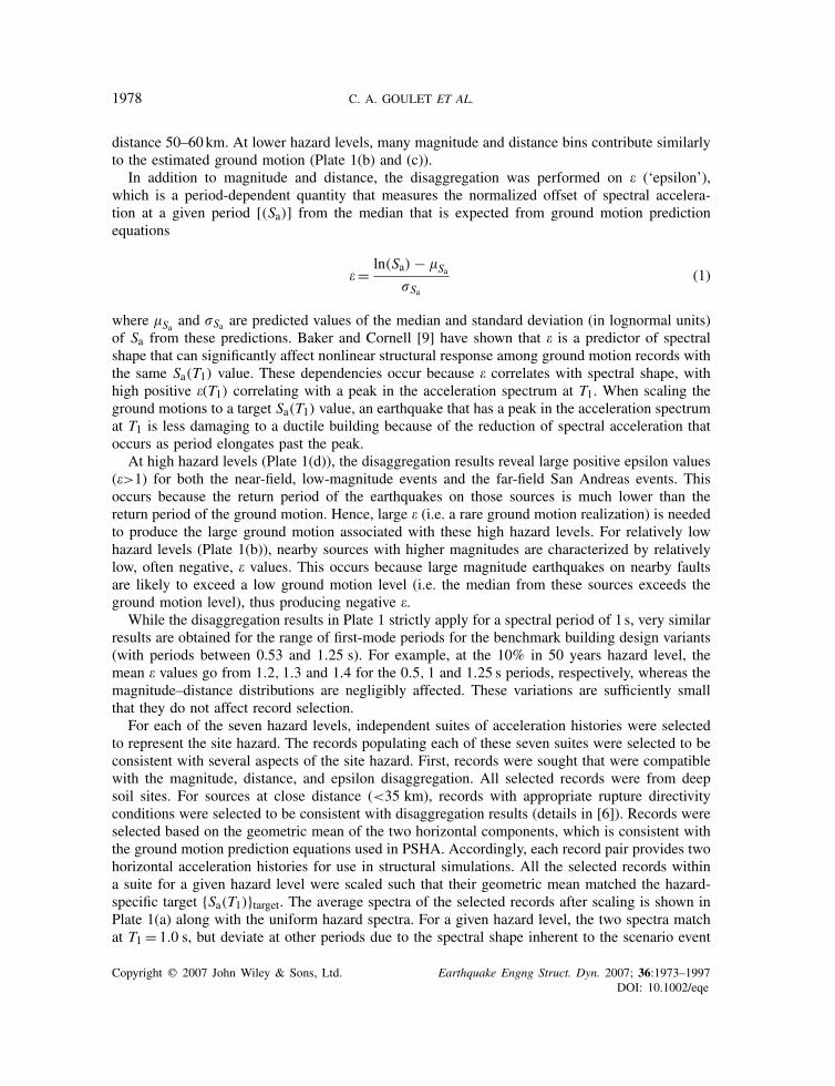
As shown in Figure 3(a), plastic hinge models for beam columns have a trilinear backbone curvedescribed by five parameters (My, �y, Ks, �cap, and Kc). Figure 3(b) shows an example of calibra-tion of this model to test data; this shows the observed hysteretic response, the calibrated hystereticresponse, and the calibrated monotonic backbone curve [12, 13]. This model was developed byIbarra et al. [14] and Ibarra [15]. The negative branch of the post-peak response simulates strain-softening behaviour associated with phenomena such as concrete crushing and rebar buckling andfracture; the accuracy of the onset and slope of this negative branch is the most critical aspectof collapse modelling [6, 14, 15]. The model captures the four important modes of cyclic strengthand stiffness degradation; this is based on an energy dissipation capacity and a term that describeshow the deterioration rate changes as damage accumulates.

Model parameters for RC beam columns are based on recommendations from Fardis and Biskinis[16] and Panagiotakos and Fardis [17] (for initial stiffness and deformation capacity) and from



0.02 0.04 0.06 0.08 0.1

0

100

−100

−200

−300−0.1 −0.08 −0.06 −0.04 −0.02 0

200

300

Shea

r Fo

rce

(kN

)

Column Drift (displacement/height)

Experimental ResultsModel Prediction

0

0.2

0.4

0.6

0.8

1

1.2

1.4

0 0.01 0.02 0.03 0.04 0.05 0.06 0.07 0.08

Chord Rotation (radians)

Nor

mal

ized

Mom

ent (

M/M

y) Kc

cappl

Ks

My

u,monopl

Ke

u,mono

20%str.loss

Mc

1

1

1

capy

(a)

(b)

Figure 3. Illustration of spring model with degradation: (a) monotonic backbone curve and(b) observed and calibrated responses for experimental test by Saatcioglu and Grira, specimenBG-6 [12], solid black line is calibrated monotonic backbone. Calibration completed as part

of the benchmark study [6] and a more extensive calibration study [13].

our own calibrations to test data using the PEER structural performance database [6, 18] whichwas developed by Berry and Eberhard. The modelling parameters are briefly summarized here,but [13] includes the most updated and complete element modelling recommendations.

Typical mean capping rotations are �plcap = 0.05 radians for columns and �plcap = 0.07 radiansfor slender beams, with a coefficient of variation of 0.60. These relatively large plastic rotationcapacities result from low axial loads, closely spaced stirrups providing shear reinforcement andconfinement, and bond-slip deformations.

Initial stiffness of plastic hinges (Ke) is defined using both the secant stiffness through the yieldpoint (i.e. Ke taken as Kyld) and the secant stiffness through 40% of the yield moment (i.e. Ke taken



as Kstf). Stiffness values Kyld and Kstf are estimated using both predictions from Panagiotakos andFardis [17] and calibrations from the PEER database [6, 13, 18]. For example, Panagiotakosand Fardis [17] predict an average Kyld of 0.2EIg for low levels of axial load. Our calibra-tions show that Kstf is about twice Kyld, and the mean inelastic hardening and softening slopesof Ks/Kyld ≈ 4% and Kc/Kyld ≈ − 8%, respectively. Our calibrations also provided guidance forcyclic deterioration parameters [6, 13].

5.3. Static pushover analysis

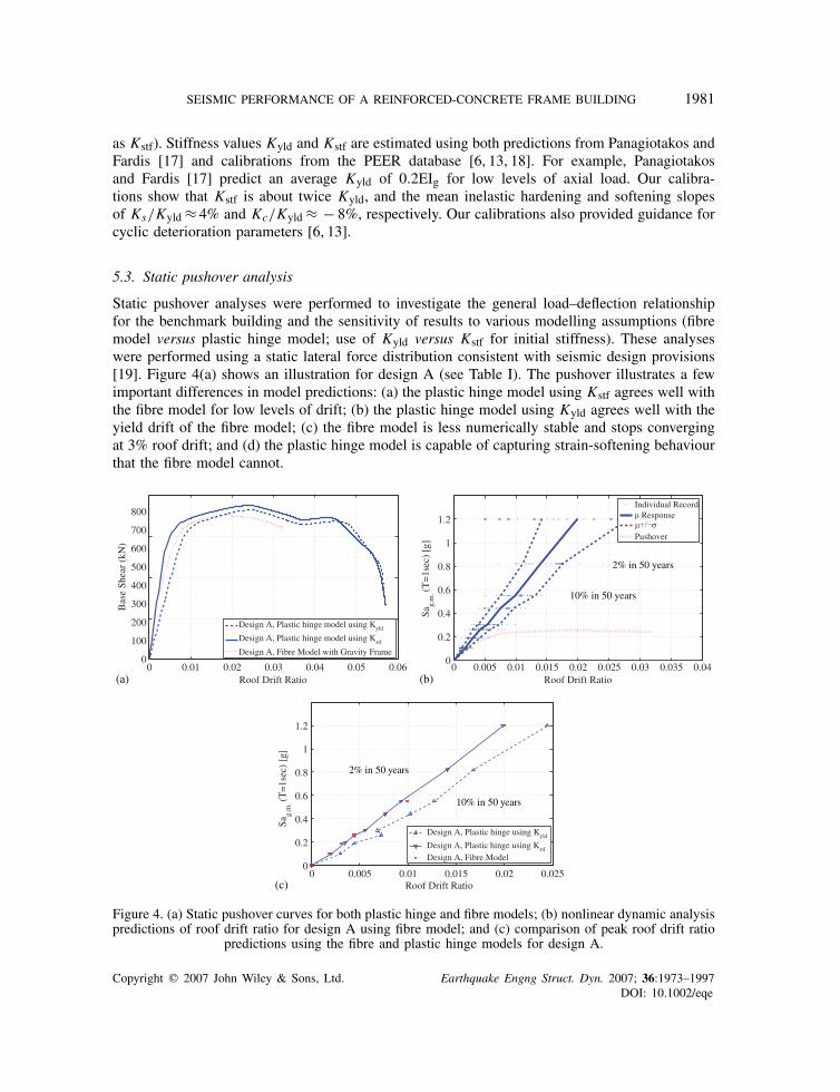
Static pushover analyses were performed to investigate the general load–deflection relationshipfor the benchmark building and the sensitivity of results to various modelling assumptions (fibremodel versus plastic hinge model; use of Kyld versus Kstf for initial stiffness). These analyseswere performed using a static lateral force distribution consistent with seismic design provisions[19]. Figure 4(a) shows an illustration for design A (see Table I). The pushover illustrates a fewimportant differences in model predictions: (a) the plastic hinge model using Kstf agrees well withthe fibre model for low levels of drift; (b) the plastic hinge model using Kyld agrees well with theyield drift of the fibre model; (c) the fibre model is less numerically stable and stops convergingat 3% roof drift; and (d) the plastic hinge model is capable of capturing strain-softening behaviourthat the fibre model cannot.

0 0.005 0.01 0.015 0.02 0.025 0.03 0.035 0.040

0.2

0.4

0.6

0.8

1

1.2

Sag.

m. (T

=1s

ec)

[g]

Roof Drift Ratio0 0.01 0.02 0.03 0.04 0.05 0.06

Roof Drift Ratio

0

100

200

300

400

500

600

700

800

Bas

e Sh

ear

(kN

)

0 0.005 0.01 0.015 0.02 0.0250

0.2

0.4

0.6

0.8

1

1.2

Sag.

m. (T

=1s

ec)

[g]

Roof Drift Ratio

Individual Record

Pushover

Response

10% in 50 years

2% in 50 years

10% in 50 years

2% in 50 years

(a)

(c)

(b)

Figure 4. (a) Static pushover curves for both plastic hinge and fibre models; (b) nonlinear dynamic analysispredictions of roof drift ratio for design A using fibre model; and (c) comparison of peak roof drift ratio

predictions using the fibre and plastic hinge models for design A.


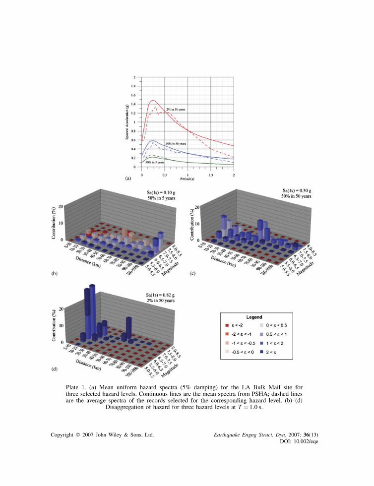
Plate 1. (a) Mean uniform hazard spectra (5% damping) for the LA Bulk Mail site forthree selected hazard levels. Continuous lines are the mean spectra from PSHA; dashed linesare the average spectra of the records selected for the corresponding hazard level. (b)–(d)

Disaggregation of hazard for three hazard levels at T = 1.0 s.

Copyright q 2007 John Wiley & Sons, Ltd. Earthquake Engng Struct. Dyn. 2007; 36(13)DOI: 10.002/eqe


5.4. Nonlinear dynamic analysis—pre-collapse response

Nonlinear dynamic analyses were performed for the benchmark building designs using groundmotion suites for each of the seven selected intensity levels (three are shown in Plate 1(a)), withan additional intensity level of 1.5 of the 2%-in-50-year ground motion. Figure 4(b) shows resultsfor the fibre model while Figure 4(c) compares the fibre model to the plastic hinge model with thetwo definitions of effective initial stiffness. The static pushover, converted to equivalent spectralacceleration, is also shown for reference [20].

The results in Figure 4(b) and (c) show the roof drift ratio plotted as a function of geometricmean Sa(T1). The small dots represent the responses from each ground motion component; and thesolid and dashed lines represent the mean and mean ± 1 standard deviation (assuming a lognormaldistribution) responses. Figure 4(b) shows that mean roof drift ratios are 1.0 and 1.4% for the10%- and the 2%-in-50-year ground motion levels, respectively.

This figure also shows that the mean dynamic analysis results obey the equal displacementrule‡ up to the 2% roof drift-level demands, corresponding to shaking 1.5 times larger than the2%-in-50-year level.

Figure 4(c) compares the mean roof drifts predicted using the fibre and plastic hinge modelswith the two treatments of initial stiffness. The results show that the plastic hinge model can predictroof drifts consistent with the fibre model only when the larger effective initial stiffness (Kstf)is used. The lower stiffness (Kyld) results in an increase of roof drift by 20–25%, which affectsmonetary loss predictions, as shown below. The larger initial stiffness definition (Kstf) should beused in the plastic hinge model for the drift predictions to be consistent with those of the fibremodel.

5.5. Nonlinear dynamic analysis—collapse simulation

To investigate sidesway collapse, incremental dynamic analyses (IDA) [21] were performed forthe benchmark designs. IDA involves increased amplitude scaling of individual ground motionrecords to estimate both: (a) the relationship between IM (in this case Sa(T1 = 1.0 s)) and EDP;and (b) the IM level that causes sidesway collapse; this study uses IDA only for predicting thiscollapse IM level. With the goal to evaluate collapse performance, the IDA was performed usingthe 34 records chosen for the 2%-in-50-year level. Collapse behaviour at ground motion levelsstronger than the 2%-in-50-year level can only be simulated using IDA, because we lack recordsfor these less-frequent ground motions.

For the IDA simulations, sidesway collapse is defined as the point of dynamic instability wheninterstorey drift increases without bound. Figure 5(a) shows IDA results from all 68 ground motioncomponents (34 records with two components each), while Figure 5(b) shows the results obtainedusing only the horizontal component of each record pair that first causes collapse; results in thesefigures are for design A. The governing component results from the two-dimensional analyses(Figure 5(b)) are considered reflective of the building collapse behaviour, assuming that the actual(three-dimensional) building will collapse in the more critical of two orthogonal directions when

‡ The equal displacement rule says that the displacement of the nonlinear structure is equal to that of a linear elasticstructure subjected to the same ground motion. This rule typically holds for structures that maintain a positivepost-yield stiffness and do not have a short period.



0 0.05 0.1 0.150

1

2

3

4

5

6Sa

g.m

.(T=

1.0s

)[g]

0

1

2

3

4

5

6

Sag.

m.(T

=1.

0s)[

g]

Maximum Interstorey Drift Ratio0 0.05 0.1 0.15

Maximum Interstorey Drift Ratio

0 0.5 1 1.5 2 2.5 3 3.5 4 4.5 50

0.1

0.2

0.3

0.4

0.5

0.6

0.7

0.8

0.9

1

P[co

llaps

e]

0 1 2 3 4 50

0.1

0.2

0.3

0.4

0.5

0.6

0.7

0.8

0.9

1

Sag.m.(T=1.0s) [g]

P[co

llaps

e]

2% in 50 year Sa = 0.82g

Sag.m.(T=1.0s) [g]

(a) (b)

(c) (d)

Figure 5. Incremental dynamic analysis for design A, using: (a) both horizontal components of groundmotion; (b) the horizontal component that first causes collapse; (c) effect of epsilon (spectral shape) on

collapse capacity; and (d) collapse CDFs including and excluding modelling uncertainty.

subjected to the three-dimensional earthquake ground motion.§ Comparison of Figure 5(a) and (b)shows a 30% lower median collapse capacity (Sacol), and a 20% lower dispersion (�LN,RTR), whenonly the more critical horizontal ground motion component is used.

5.5.1. Effects of spectral shape (epsilon). The results shown in Figure 5(a) and (b) are for theground motion suite developed above for the 2%-in-50-year ground motion level, in which � isaccounted for during the selection process; this is termed ‘Set One’ and the mean value of �(1 s)is 1.4 for this data set. We also selected an alternative ground motion record set and performedadditional analyses to investigate the effect of � on the predicted collapse capacity; this ‘Set Two’was selected without regard to � and has a mean �(1 s) = 0.4.

The collapse Sa(T1) capacities from Figure 5(b) are plotted as a cumulative distribution function(CDF) in Figure 5(c) (Set One). Superimposed in Figure 5(c) are similar collapse capacities from

§This approximate method considers only the differences between the two horizontal components of ground motion,not three-dimensional structural interactions (for the buildings considered in this study, three-dimensional effectsshould not be significant for perimeter frames, but would be significant for space frame designs).



an IDA using ground motions with lower � (Set Two). Figure 5(c) shows that a change fromSet One to Set Two decreases the expected (median) collapse capacity by 20%, meaning that ifone ignores epsilon, one would underestimate collapse capacity. A similar comparison using bothhorizontal components of ground motion on the benchmark structure instead shows a 40% shiftin the median.

Two recent studies provide a comparison to the results shown here. Zareian [22] found thata change from �= 0 to +2.0 caused an approximate 50–70% increase in the expected collapsecapacity. Haselton and Baker [23] found that a change consistent with Set One versus Set Twocauses a 50% shift in median collapse capacity. Results from both of the above studies arecomparable with the 40% median shift found in this study.

This shift in the collapse capacity CDF profoundly affects the mean rate of collapse, whichdepends on the position of the collapse CDF with respect to the hazard curve. For this buildingwhere the extreme tail of the hazard curve dominates the collapse rate, a 20% increase in themedian collapse capacity causes the mean annual frequency of collapse to decrease by a factorof 5–7 [24]. Similarly, a 40% increase in capacity would decrease the mean annual frequency ofcollapse by a factor of around 10. These results demonstrate the importance of ground motionacceleration history selection criteria in accurately predicting building collapse capacity.

5.5.2. Effects of structural modelling uncertainties. The collapse capacity CDF using Set Oneground motions is re-plotted as the solid line in Figure 5(d), where the data points and fitted CDFare for analyses that only reflect the record-to-record variability. The variability in collapse capacityarising from uncertain structural properties was also investigated, and this section explains howwe developed the dashed CDF in Figure 5(d).

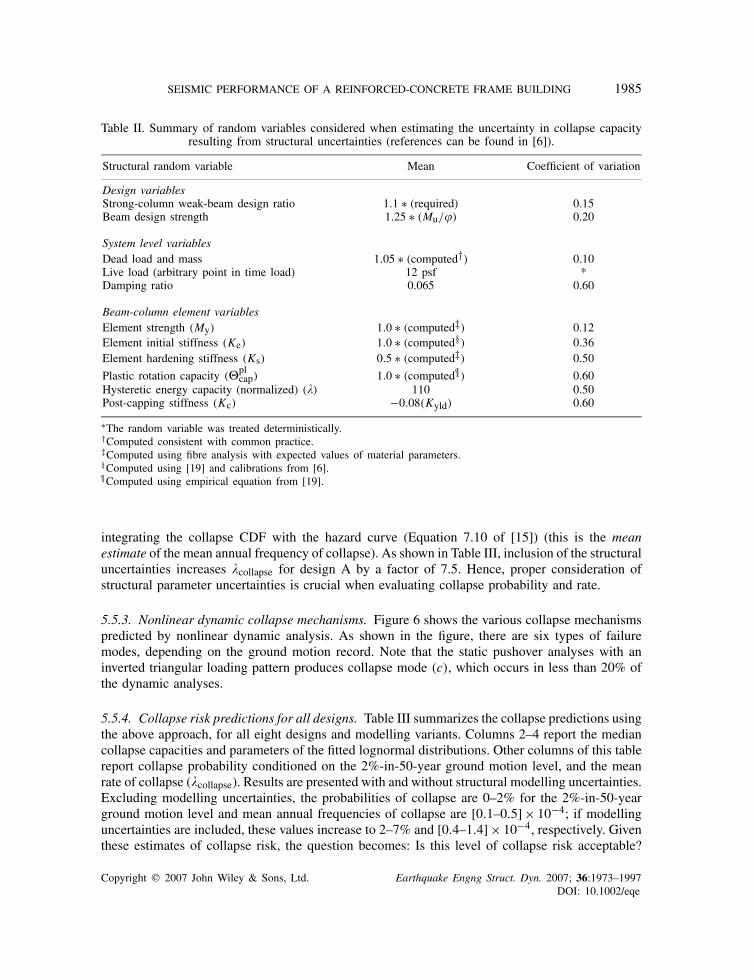
Table II summarizes the structural parameters for which uncertainties were considered in thedynamic response analyses. Many of these parameters were previously defined in Figure 3(a).Table II shows that variations in some of the parameters are large (e.g. the coefficient of variationin the plastic rotation capacity and degradation parameters is on the order of 0.5–0.6). The first-order second-moment method [25] was used to propagate these structural uncertainties and toestimate the resulting uncertainty in collapse capacity. Correlations between the uncertain structuralparameters were considered and found to be important. Using reasonable correlation assumptions,the uncertainty in collapse capacity is a standard deviation of 0.5, in natural log units. Thisrather large value reflects the large variation in some of the underlying modelling parametersthat significantly affect the collapse simulation (Table II). The primary factors that drive the 0.5value is the uncertainty in element plastic rotation capacity and the correlations among modellingparameters for a given element as well as element-to-element correlations in properties [6].

To incorporate the effects of structural uncertainties, we use the mean estimate method, incontrast to an estimate at a given level of prediction confidence, which effectively combines bothrecord-to-record and structural variability into a single aggregate value. This results in a total logstandard deviation of 0.58; this is indicated by the dashed line in Figure 5(d). We offer this valuecautiously, since it is based on a first-order approximation and only design A. We believe thatfurther study is required to confirm or improve our estimate.

Even though the mean estimate method does not result in a shift in the median collapse point,the increased variation has a significant effect on collapse probabilities in the lower tail of thedistribution. For example, at the 2%-in-50-year ground motion level, the probability of collapseis 0–2% with only record-to-record variability and 2–7% when structural modelling uncertaintiesare also included. We also compute a mean annual frequency of collapse (�collapse) by numerically



Table II. Summary of random variables considered when estimating the uncertainty in collapse capacityresulting from structural uncertainties (references can be found in [6]).

Structural random variable Mean Coefficient of variation

Design variablesStrong-column weak-beam design ratio 1.1 ∗ (required) 0.15Beam design strength 1.25 ∗ (Mu/�) 0.20

System level variablesDead load and mass 1.05 ∗ (computed†) 0.10Live load (arbitrary point in time load) 12 psf *Damping ratio 0.065 0.60

Beam-column element variablesElement strength (My) 1.0 ∗ (computed‡) 0.12Element initial stiffness (Ke) 1.0 ∗ (computed§ ) 0.36Element hardening stiffness (Ks) 0.5 ∗ (computed‡) 0.50

Plastic rotation capacity (�plcap) 1.0 ∗ (computed¶ ) 0.60

Hysteretic energy capacity (normalized) (�) 110 0.50Post-capping stiffness (Kc) −0.08(Kyld) 0.60

∗The random variable was treated deterministically.†Computed consistent with common practice.‡Computed using fibre analysis with expected values of material parameters.§Computed using [19] and calibrations from [6].¶Computed using empirical equation from [19].

integrating the collapse CDF with the hazard curve (Equation 7.10 of [15]) (this is the meanestimate of the mean annual frequency of collapse). As shown in Table III, inclusion of the structuraluncertainties increases �collapse for design A by a factor of 7.5. Hence, proper consideration ofstructural parameter uncertainties is crucial when evaluating collapse probability and rate.

5.5.3. Nonlinear dynamic collapse mechanisms. Figure 6 shows the various collapse mechanismspredicted by nonlinear dynamic analysis. As shown in the figure, there are six types of failuremodes, depending on the ground motion record. Note that the static pushover analyses with aninverted triangular loading pattern produces collapse mode (c), which occurs in less than 20% ofthe dynamic analyses.

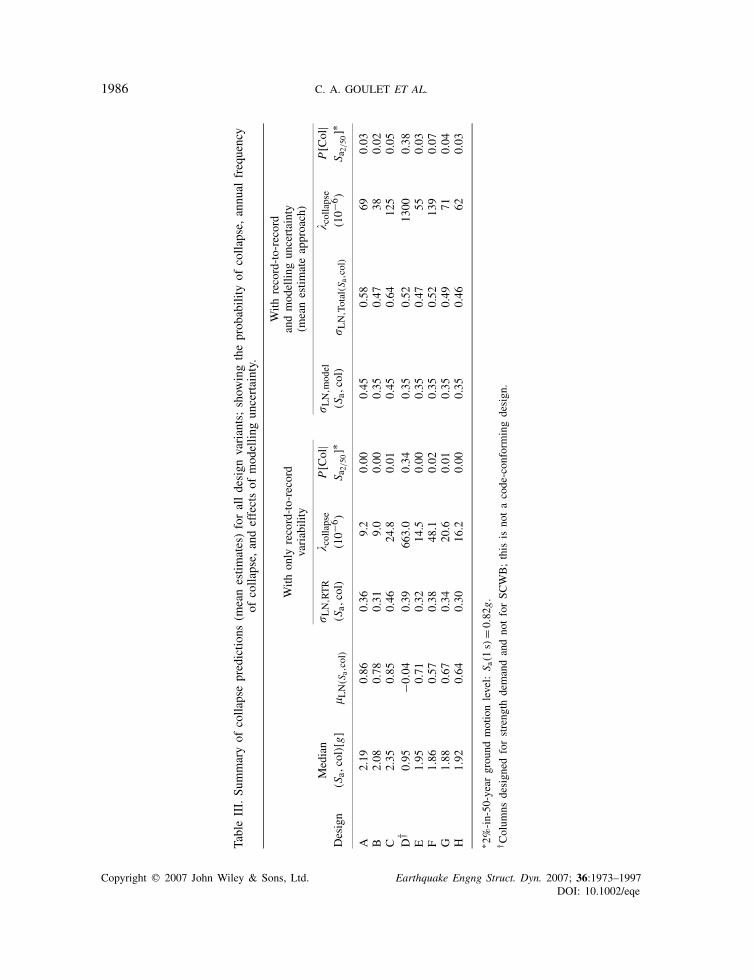
5.5.4. Collapse risk predictions for all designs. Table III summarizes the collapse predictions usingthe above approach, for all eight designs and modelling variants. Columns 2–4 report the mediancollapse capacities and parameters of the fitted lognormal distributions. Other columns of this tablereport collapse probability conditioned on the 2%-in-50-year ground motion level, and the meanrate of collapse (�collapse). Results are presented with and without structural modelling uncertainties.Excluding modelling uncertainties, the probabilities of collapse are 0–2% for the 2%-in-50-yearground motion level and mean annual frequencies of collapse are [0.1–0.5]× 10−4; if modellinguncertainties are included, these values increase to 2–7% and [0.4–1.4] × 10−4, respectively. Giventhese estimates of collapse risk, the question becomes: Is this level of collapse risk acceptable?



TableIII.Su

mmaryof

collapsepredictio

ns(m

eanestim

ates)foralldesign

variants;show

ingtheprobability

ofcollapse,

annual

frequency

ofcollapse,

andeffectsof

modellin

guncertainty.

With

record-to-record

With

only

record-to-record

andmod

ellin

gun

certainty

variability

(meanestim

ateapproach)

Median

� LN

,RTR

� collapse

P[C

ol|

� LN

,mod

el� c

ollapse

P[C

ol|

Design

(Sa,col)[g]

� LN

(Sa,col)

(Sa,col)

(10−

6)

S a2/50

]∗(S

a,col)

� LN

,Total

(Sa,col)

(10−

6)

S a2/50

]∗

A2.19

0.86

0.36

9.2

0.00

0.45

0.58

690.03

B2.08

0.78

0.31

9.0

0.00

0.35

0.47

380.02

C2.35

0.85

0.46

24.8

0.01

0.45

0.64

125

0.05

D†

0.95

−0.04

0.39

663.0

0.34

0.35

0.52

1300

0.38

E1.95

0.71

0.32

14.5

0.00

0.35

0.47

550.03

F1.86

0.57

0.38

48.1

0.02

0.35

0.52

139

0.07

G1.88

0.67

0.34

20.6

0.01

0.35

0.49

710.04

H1.92

0.64

0.30

16.2

0.00

0.35

0.46

620.03

∗ 2%-in-50

-yeargrou

ndmotionlevel:S a

(1s)

=0.82

g.† C

olum

nsdesign

edforstreng

thdemandandno

tforSC

WB;this

isno

tacode-con

form

ingdesign

.



(a) 40% of collapses (b) 27% of collapses

(c) 17% of collapses (d) 12% of collapses

(e) 5% of collapses (f) 2% of collapses

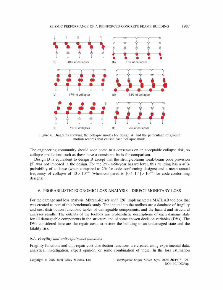
Figure 6. Diagrams showing the collapse modes for design A, and the percentage of groundmotion records that caused each collapse mode.

The engineering community should soon come to a consensus on an acceptable collapse risk, socollapse predictions such as these have a consistent basis for comparison.

Design D is equivalent to design B except that the strong-column weak-beam code provision[5] was not imposed in the design. For the 2%-in-50-year hazard level, this building has a 40%probability of collapse (when compared to 2% for code-conforming designs) and a mean annualfrequency of collapse of 13× 10−4 (when compared to [0.4–1.4]× 10−4 for code-conformingdesigns).

6. PROBABILISTIC ECONOMIC LOSS ANALYSIS—DIRECT MONETARY LOSS

For the damage and loss analysis, Mitrani-Reiser et al. [26] implemented a MATLAB toolbox thatwas created as part of this benchmark study. The inputs into the toolbox are a database of fragilityand cost distribution functions, tables of damageable components, and the hazard and structuralanalyses results. The outputs of the toolbox are probabilistic descriptions of each damage statefor all damageable components in the structure and of some chosen decision variables (DVs). TheDVs considered here are the repair costs to restore the building to an undamaged state and thefatality risk.

6.1. Fragility and unit-repair-cost functions

Fragility functions and unit-repair-cost distribution functions are created using experimental data,analytical investigation, expert opinion, or some combination of these. In the loss estimation



Table IV. Summary of assembly fragility and cost distribution parameters.

Fragility parameters Repair-cost parameters

Assembly description Unit EDP Damage state xm � xm($) �

Ductile CIP RC beams ea DDI Light 0.08 1.36 8000 0.42Ductile CIP RC beams ea DDI Moderate 0.31 0.89 22 500 0.40Ductile CIP RC beams ea DDI Severe 0.71 0.80 34 300 0.37Ductile CIP RC beams ea DDI Collapse 1.28 0.74 34 300 0.37Ductile CIP RC columns ea DDI Light 0.08 1.36 8000 0.42Ductile CIP RC columns ea DDI Moderate 0.31 0.89 22 500 0.40Ductile CIP RC columns ea DDI Severe 0.71 0.80 34 300 0.37Ductile CIP RC columns ea DDI Collapse 1.28 0.74 34 300 0.37Column–slab ea IDR Light cracking 0.0030 0.40 35 0.20connectionsColumn–slab ea IDR Severe cracking 0.0100 0.30 435 0.20connectionsColumn–slab ea IDR Punching 0.0145 0.60 3273 0.20connections shear failureDrywall partition 64 ft2 IDR Visible 0.0039 0.17 88 0.20Drywall partition 64 ft2 IDR Significant 0.0085 0.23 525 0.20Drywall finish 64 ft2 IDR Visible 0.0039 0.17 88 0.20Drywall finish 64 ft2 IDR Significant 0.0085 0.23 253 0.20Exterior glazing pane IDR Crack 0.040 0.36 439 0.26Exterior glazing pane IDR Fallout 0.046 0.33 439 0.26Acoustical ceiling ft2 PDA Collapse 92/(l + w) 0.81 2.21 ∗ A 0.50Automatic sprinklers 12 ft PDA Fracture 32 1.4 900 0.50

DDI, deformation damage index portion of the Park-Ang damage index; IDR, interstorey drift ratio; PDA, peakdiaphragm acceleration; l, room length; w, room width; A, room area.

literature, lognormal distributions are commonly used to quantify the uncertainty in the unit repaircosts and fragility corresponding to the various damage states for each damageable structuraland non-structural assembly [4, 27, 28]. Therefore, the median capacity and logarithmic standarddeviations of capacity (defined in terms of the EDP value that causes an assembly to reach orexceed a given damage state) are used to create the fragility functions, and then to estimate damage.The corresponding medians and logarithmic standard deviations of associated unit repair costs foreach damage state of an assembly are used to define the unit-repair-cost distribution functions forthe loss assessment. Existing and new fragility functions and unit-repair-cost functions that areused in this study are summarized in Table IV, where xm and � denote the median and logarithmicstandard deviation, respectively. This table lists the structural and non-structural components ofthe benchmark building and the EDPs used the damage analysis; additional information for eachof these components is available in [6].

6.2. Damage analysis

The structural analysis results are combined with the damageable component fragility func-tions, using the law of total probability, to compute the probability of reaching or exceedingdamage state j for a component of type i , conditioned on the structure not collapsing (NC)



.1 .19 .26 .3 .44 .55 .82 1.20

0.5

1

1.5

Spectral Acceleration (g)

Mea

n R

epai

r C

ost (

$M)

BeamsColumnsPartitionsPaintGlazingCol-Slab JointsSprinklersCeiling

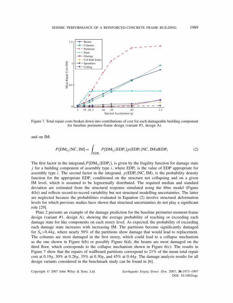
Figure 7. Total repair costs broken down into contributions of cost for each damageable building componentfor baseline perimeter-frame design (variant #1, design A).

and on IM:

P[DMi j |NC, IM] =∫EDPi

P[DMi j |EDPi ]p(EDPi |NC, IM)dEDPi (2)

The first factor in the integrand,P[DMi j |EDPi ], is given by the fragility function for damage statej for a building component of assembly type i , where EDPi is the value of EDP appropriate forassembly type i . The second factor in the integrand, p(EDPi |NC, IM), is the probability densityfunction for the appropriate EDP, conditioned on the structure not collapsing and on a givenIM level, which is assumed to be lognormally distributed. The required median and standarddeviation are estimated from the structural response simulated using the fibre model (Figure4(b)) and reflects record-to-record variability but not structural modelling uncertainties. The latterare neglected because the probabilities evaluated in Equation (2) involve structural deformationlevels for which previous studies have shown that structural uncertainties do not play a significantrole [29].

Plate 2 presents an example of the damage prediction for the baseline perimeter-moment-framedesign (variant #1, design A), showing the average probability of reaching or exceeding eachdamage state for like components on each storey level. As expected, the probability of exceedingeach damage state increases with increasing IM. The partitions become significantly damagedfor Sa>0.44g, where nearly 50% of the partitions show damage that would lead to replacement.The columns are most damaged in the first storey, which could lead to a collapse mechanismas the one shown in Figure 6(b) or possibly Figure 6(d); the beams are most damaged on thethird floor, which corresponds to the collapse mechanism shown in Figure 6(c). The results inFigure 7 show that the repairs of wallboard partitions correspond to 21% of the mean total repaircost at 0.19g, 30% at 0.26g, 35% at 0.30g, and 45% at 0.44g. The damage analysis results for alldesign variants considered in the benchmark study can be found in [6].


none light moderate severe collapse none visible signif.

Columns Beams Partitions Story

1

2

3

4


Ave

rage

Pro

babi

lity

.1 .19 .26 .3 .44 .55 .82 1.20

0.5

1

.1 .19 .26 .3 .44 .55 .82 1.20

0.5

1

.1 .19 .26 .3 .44 .55 .82 1.20

0.5

1

.1 .19 .26 .3 .44 .55 .82 1.20

0.5

1

.1 .19 .26 .3 .44 .55 .82 1.20

0.5

1

.1 .19 .26 .3 .44 .55 .82 1.20

0.5

1

.1 .19 .26 .3 .44 .55 .82 1.20

0.5

1

.1 .19 .26 .3 .44 .55 .82 1.20

0.5

1

.1 .19 .26 .3 .44 .55 .82 1.20

0.5

1

.1 .19 .26 .3 .44 .55 .82 1.20

0.5

1.1 .19 .26 .3 .44 .55 .82 1.2

0

0.5

1

.1 .19 .26 .3 .44 .55 .82 1.20

0.5

1

Plate 2. Average probabilities of damage per storey level for baselineperimeter-frame design (variant #1, design A).

Copyright q 2007 John Wiley & Sons, Ltd. Earthquake Engng Struct. Dyn. 2007; 36(13)DOI: 10.002/eqe


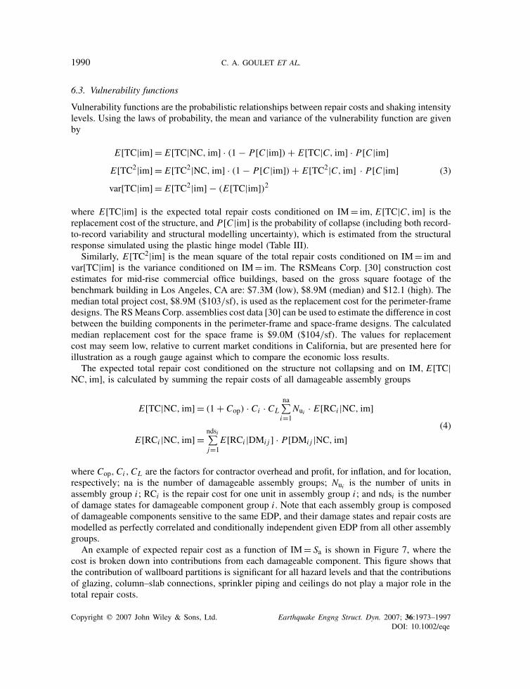
6.3. Vulnerability functions

Vulnerability functions are the probabilistic relationships between repair costs and shaking intensitylevels. Using the laws of probability, the mean and variance of the vulnerability function are givenby

E[TC|im] = E[TC|NC, im] · (1 − P[C |im]) + E[TC|C, im] · P[C |im]E[TC2|im] = E[TC2|NC, im] · (1 − P[C |im]) + E[TC2|C, im] · P[C |im]var[TC|im] = E[TC2|im] − (E[TC|im])2

(3)

where E[TC|im] is the expected total repair costs conditioned on IM= im, E[TC|C, im] is thereplacement cost of the structure, and P[C |im] is the probability of collapse (including both record-to-record variability and structural modelling uncertainty), which is estimated from the structuralresponse simulated using the plastic hinge model (Table III).

Similarly, E[TC2|im] is the mean square of the total repair costs conditioned on IM= im andvar[TC|im] is the variance conditioned on IM= im. The RSMeans Corp. [30] construction costestimates for mid-rise commercial office buildings, based on the gross square footage of thebenchmark building in Los Angeles, CA are: $7.3M (low), $8.9M (median) and $12.1 (high). Themedian total project cost, $8.9M ($103/sf), is used as the replacement cost for the perimeter-framedesigns. The RSMeans Corp. assemblies cost data [30] can be used to estimate the difference in costbetween the building components in the perimeter-frame and space-frame designs. The calculatedmedian replacement cost for the space frame is $9.0M ($104/sf). The values for replacementcost may seem low, relative to current market conditions in California, but are presented here forillustration as a rough gauge against which to compare the economic loss results.

The expected total repair cost conditioned on the structure not collapsing and on IM, E[TC|NC, im], is calculated by summing the repair costs of all damageable assembly groups

E[TC|NC, im] = (1 + Cop) · Ci · CL

na∑i=1

Nui · E[RCi |NC, im]

E[RCi |NC, im] =ndsi∑j=1

E[RCi |DMi j ] · P[DMi j |NC, im](4)

where Cop,Ci ,CL are the factors for contractor overhead and profit, for inflation, and for location,respectively; na is the number of damageable assembly groups; Nui is the number of units inassembly group i ; RCi is the repair cost for one unit in assembly group i ; and ndsi is the numberof damage states for damageable component group i . Note that each assembly group is composedof damageable components sensitive to the same EDP, and their damage states and repair costs aremodelled as perfectly correlated and conditionally independent given EDP from all other assemblygroups.

An example of expected repair cost as a function of IM= Sa is shown in Figure 7, where thecost is broken down into contributions from each damageable component. This figure shows thatthe contribution of wallboard partitions is significant for all hazard levels and that the contributionsof glazing, column–slab connections, sprinkler piping and ceilings do not play a major role in thetotal repair costs.



.1 .19 .3 .44 .55 .82 1.20

1

2

3

4

5

6

7


Mea

n R

epai

r C

ost (

$M)

Design A, Fibre Model of Perimeter FrameDesign E, Fibre Model of Space Frame

10% in 50 yrs 2% in 50 yrs

.26

0

1

2

3

4

5

6


Mea

n R

epai

r C

ost (

$M)

0

0.1

0.2

0.3

0.4

0.5

0.6

Mea

n D

amag

e Fa

ctor

Design A, Fibre Model with Gravity FrameDesign A, Plastic Hinge Model using Kyld

Design A, Plastic Hinge Model using Kstf

10% in 50 yrs 2% in 50 yrs

.1 .19 .3 .44 .55 .82 1.2.26

(a)

(b)

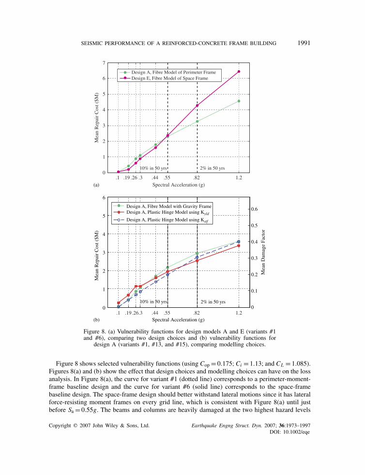
Figure 8. (a) Vulnerability functions for design models A and E (variants #1and #6), comparing two design choices and (b) vulnerability functions for

design A (variants #1, #13, and #15), comparing modelling choices.

Figure 8 shows selected vulnerability functions (using Cop = 0.175;Ci = 1.13; and CL = 1.085).Figures 8(a) and (b) show the effect that design choices and modelling choices can have on the lossanalysis. In Figure 8(a), the curve for variant #1 (dotted line) corresponds to a perimeter-moment-frame baseline design and the curve for variant #6 (solid line) corresponds to the space-framebaseline design. The space-frame design should better withstand lateral motions since it has lateralforce-resisting moment frames on every grid line, which is consistent with Figure 8(a) until justbefore Sa = 0.55g. The beams and columns are heavily damaged at the two highest hazard levels



for simulation (Sa = 0.82 and 1.2g) and because there are more of them to repair in the space-framedesign than in the perimeter-frame design, their contributions to the total repair cost dominate thecontributions of the other damageable components. In fact, the contribution to mean total repaircost from the beams surpasses that of the partitions in the space-frame design at all levels of Sa,which does not occur in any of the perimeter-frame variants.

In Figure 8(b), the curve for variant #13 (solid line) corresponds to the baseline perimeter-moment-frame design using a plastic hinge model with initial stiffness defined as the secantstiffness through the yield point (Kyld); the curve for variant #15 (dashed line) corresponds to asimilar design except that the initial stiffness is defined as the secant stiffness corresponding to40% of the yield moment (Kstf); variant #1 (dotted line) is given again in this plot to comparethe baseline fibre model with these plastic hinge models. Note that the fibre model results areconsistent with the ones from the plastic hinge model using Kstf until Sa = 0.19g, where the twocurves diverge and the mean total repair costs become greater than for the fibre model for allvalues of Sa>0.19g. This is consistent with the behaviour shown in the static pushover curvesof Figure 4(a). A summary of the variants considered in this study is shown in Table V and thecorresponding means and coefficients of variation of the total repair costs are given for each levelof Sa.

6.4. Expected annual loss

The expected annual loss (EAL) is a valuable result for property stakeholders, which accounts forthe frequency and severity of various seismic events. EAL is calculated as the product of the meantotal rate of occurrence of events of interest and the mean loss conditional on an event of interestoccurring [25, 31], which may be expressed as

EAL= 0

∫ ∞

im0

E[TC|im]p(im|IM�im0)dim (5)

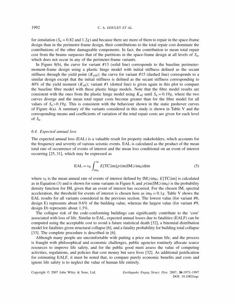
where 0 is the mean annual rate of events of interest defined by IM�im0; E[TC|im] is calculatedas in Equation (3) and is shown for some variants in Figure 8; and p(im|IM�im0) is the probabilitydensity function for IM, given that an event of interest has occurred. For the chosen IM, spectralacceleration, the threshold for events of interest is chosen here as im0 = 0.1g. Table V shows theEAL results for all variants considered in the previous section. The lowest value (for variant #6,design E) represents about 0.6% of the building value, whereas the largest value (for variant #9,design D) represents about 1.3%.

The collapse risk of the code-conforming buildings can significantly contribute to the ‘cost’associated with loss of life. Similar to EAL, expected annual losses due to fatalities (EALF) can becomputed using the acceptable cost to avoid a future statistical death [32], a binomial distributionmodel for fatalities given structural collapse [6], and a fatality probability for building total collapse[33]. The complete procedure is described in [6].

Although many people are uncomfortable with putting a price on human life, and the processis fraught with philosophical and economic challenges, public agencies routinely allocate scarceresources to improve life safety, and for the public good must assess the value of competingactivities, regulations, and policies that cost money but save lives [32]. As additional justificationfor estimating EALF, it must be noted that, to compare purely economic benefits and costs andignore life safety is to neglect the value of human life entirely.



Table V. Design variant descriptions and corresponding EAL results.

Variant number, design andmodel description Sa(T1) 0.1 0.19 0.26 0.3 0.44 0.55 0.82 1.2 EAL ($)

VID #1 (design A): perimeter frame,designed with expected overstrength;fibre model, concrete tensile strengthmodelled, gravity frame included

Mean 0.06 0.43 0.90 1.12 1.78 2.30 3.27 4.55 66 460COV 0.52 0.17 0.15 0.16 0.20 0.24 0.33 0.36

VID #2 (design C): same as design A,but designed with uniform beams andcolumns over height; modelled sameas VID #1

Mean 0.04 0.35 0.64 0.80 1.47 1.90 2.91 4.24 51 807COV 0.62 0.18 0.16 0.17 0.21 0.27 0.42 0.46

VID #3 (design B): same as design A,but designed with bare code-minimumstrengths; modelled same as VID #1

Mean 0.10 0.71 1.34 1.44 2.08 2.54 3.42 4.38 95 530COV 0.37 0.13 0.12 0.12 0.11 0.13 0.23 0.35

VID #6 (design E): baseline spaceframe; fibre model, concrete tensilestrength modelled

Mean 0.06 0.22 0.61 0.87 1.60 2.36 4.28 6.42 49 296COV 0.51 0.25 0.15 0.14 0.16 0.17 0.20 0.16

VID #9 (design D): same as design C,but no SCWB provision enforced (notcode conforming); modelled same asVID #1

Mean 0.13 0.80 1.51 1.64 2.62 3.40 5.31 7.17 112 810COV 0.36 0.33 0.40 0.51 0.64 0.66 0.53 0.34

VID #11 (design A): same as designA; modelled same as VID #1, butconcrete tensile strength and stiffnessnot modelled

Mean 0.12 0.70 1.19 1.34 2.00 2.46 3.26 4.71 92 596COV 0.35 0.13 0.13 0.14 0.18 0.22 0.33 0.34

VID #12 (design A): same as designA; modelled same as VID #1, butgravity frame not modelled

Mean 0.06 0.52 1.09 1.25 1.90 2.35 3.22 4.38 75 943COV 0.49 0.15 0.14 0.15 0.19 0.23 0.34 0.39

VID #13 (design A): same as designA; plastic hinge model with secantstiffness through yield (Kyld)

Mean 0.26 0.69 1.19 1.19 1.69 2.06 2.74 3.72 96 153COV 0.17 0.15 0.15 0.16 0.22 0.28 0.44 0.49

VID #14 (design A): same as designA; plastic hinge model, with secantstiffness through 60% of yield

Mean 0.12 0.63 1.07 1.13 1.68 2.10 3.02 4.40 82 307COV 0.29 0.15 0.15 0.17 0.21 0.27 0.37 0.38

VID #15 (design A): same as designA; plastic hinge model with secantstiffness through 40% of yield (Kstf)

Mean 0.03 0.42 0.72 0.91 1.48 1.91 3.10 4.49 57 237COV 0.75 0.17 0.17 0.19 0.25 0.30 0.36 0.37

Mean, mean total repair cost for Sa(g) in $M; COV, coefficient of variation of repair cost for Sa(g).

The expected annual number of fatalities for designs A, B, D, and E ranges between 0.001and 0.004 (EALF= $4300–$14 300, respectively), including IMs extrapolated up to Sa = 4g.The expected annual number of fatalities increases drastically to 0.05 for design D (consistentwith 0.06 reported for a post-Northridge steel moment-resisting frame building [34, 35]), which



does not include the SCWB provision. These values of EALF are expected to be conservative(meaning high) because of the various assumptions made, such as full occupancy around the clockand that all collapses are total (rather than some partial).

7. CONCLUSIONS

We have implemented a PBEE methodology to predict seismic performance of a four-storeyRC SMRF benchmark building that is designed according to the 2003 IBC [3]. Performance isquantified in terms of structural and non-structural damage, repair costs, collapse statistics, andlosses due to fatalities. Several design alternatives for the benchmark building are considered alongwith several structural modelling alternatives for a given design.

Accounting for uncertainties in both structural modelling and record-to-record variability, col-lapse probabilities lie in the range 2–7% for earthquake ground motions with a 2% probability ofexceedance in 50 years. Combining the ground motion hazard with the collapse predictions, wefind mean frequencies of collapse of [0.4–1.4]× 10−4 for the various benchmark building designs.

Figure C1-23 from the FEMA 223 document [35] suggests that these computed collapse prob-abilities are high, compared with previous estimates on the order of 0.2–0.5% for a buildingsubjected to 2%-in-50-year ground motions. The topic of acceptable collapse risk is worthy ofsubstantial further study.

In the process of developing the above findings related to collapse, a number of importantconsiderations were revealed that are likely transferable to other buildings:

• For rare ground motions, it is critical to select ground motion records in consideration ofspectral shape. Here, this was done using parameter � from the PSHA. If � had been neglectedin our simulations, the median predicted collapse capacities would be reduced by 20–40%,which in turn increases the mean annual rate of collapse by a factor of 5–10.

• Realistic estimates of plastic rotation capacity are essential for accurate collapse predictions.Recent research and new model calibrations conducted as part of this study reveal muchlarger rotation capacities, on the order of 0.06 radians for a conforming RC element, than aregenerally assumed in modern practice (see Section 5.2).

• Collapse probability is highly sensitive to structural modelling uncertainties. The introductionof structural modelling uncertainty increased estimated collapse rates by approximately afactor of 4–8. We believe, therefore, that further study of this issue is critical.

• Different collapse mechanisms occur for different ground motions, and the mechanism pre-dicted by nonlinear static pushover analysis was not the predominant collapse mechanismobserved in the time-series response analyses.

• As expected, the structural design that did not enforce the strong-column weak-beam provisioncollapsed at lower hazard levels than the code-conforming designs. The collapse probability atthe 2%-in-50-year ground motion was 38%, when compared to 2–7% for the seven conformingdesigns. The mean annual frequency of collapse is 13× 10−4 and the mean annual numberof fatalities is 0.05, when compared to [0.4–1.4]× 10−4 and to 0.001–0.004, respectively, forthe seven conforming designs.

The potential for financial loss is considerable. Loss modelling considering the moment-framebeams and columns, the column–slab connections, the wallboard partitions, the acoustical ceiling,the sprinkler piping, the exterior glazing, and the interior paint, indicates that mean annual losses



from earthquakes are likely in the range of $52 000–$95 000 for the various code-conformingbenchmark building designs, or roughly 1% of the replacement cost of the building. Some importantlessons learned from these simulations that may be transferable to other projects include thefollowing:

• Economic losses are dominated by the expected costs of repairing the wallboard partitions,the structural members and painting the interior, in this order of importance (see Figure 7).

• Expected annual loss (EAL) estimates are highly sensitive to the manner of estimating the ini-tial stiffness of the structural elements. The EAL for the baseline perimeter-frame model usingthe fibre model is $66 500 (0.75% of replacement cost); the EAL for the same designusing the plastic hinge model with secant stiffness through yield (Kyld) is $96 200 (1.1%of replacement cost); the EAL using a secant stiffness through 60 and 40% of yield (Kstf)is $82 300, and $57 200, (0.9, and 0.6% of replacement cost), respectively. If a plastic hingeapproach is used to model the structural behaviour, the initial stiffness of the hinge elementshould be calibrated to test data and chosen carefully (similar to Kstf) to better model thebuilding stiffness under frequent ground motions.

• Losses are sensitive to other modelling choices. If the tensile strength of the concrete isignored by assuming all pre-cracked concrete (variant #11) (this changes the initial stiffnessof the element model), there is an increase of almost 40% in EAL. If the gravity frame isignored in the structural model (variant #12), thus neglecting the contribution of its strengthand stiffness, there is an increase of almost 15% in EAL.

• Variant #2 (design C), a more conservative design than variant #1 (design A) because it usesthe same beams and columns throughout the building, produces an EAL that is 22% smaller(Table V). Variant #3 (design B), a code-minimum design, produces an EAL that is 44%larger (Table V).

• The strong-column weak-beam provisions are ignored for variant #9 (design D), whichdrastically increases the EAL of the baseline model (variant #1, design A) by 70%.

• Although the mean repair costs are much higher for the space-frame designs than for theperimeter-frame designs at the two highest levels of Sa (see Figure 8(a)), the EAL and theexpected annual loss from fatalities (EALF) for the space-frame design is 25 and 33% lessthan the perimeter-frame design, respectively. This is because the mean repair costs are lowerfor the more frequent events and because the space-frame design has less risk of collapse.These reductions in EAL and EALF can be used to allow stakeholders to make trade-offsbetween the extra up-front cost (approximately $100 000) for the space-frame design [6].

ACKNOWLEDGEMENTS

This work was supported primarily by the Earthquake Engineering Research Centers Program of theNational Science Foundation, under award number EEC-9701568 through the Pacific EarthquakeEngineering Research Center (PEER). Any opinions, findings, and conclusions or recommendations ex-pressed in this material are those of the authors and do not necessarily reflect those of the National ScienceFoundation. Supplementary funding was also provided to Christine Goulet from the National Sciences andEngineering Research Council of Canada and from le Fonds quebecois de la recherche sur la nature etles technologies. The primary lead institutions for the seismic hazard analysis, the structural analysis,and the damage and loss analysis, in this PEER project are, respectively, the University of California atLos Angeles (J. Stewart (P.I.) and C. Goulet), Stanford University (G. Deierlein (P.I.) and C. Haselton)and the California Institute of Technology (J. Beck (P.I.), J. Mitrani-Reiser and K. Porter). The authors



would also like to acknowledge the valuable input from Professors Helmut Krawinkler, Allin Cornell,Eduardo Miranda, Ertugrul Taciroglu and Jack Baker; architect and professional cost estimator, Gee Heck-sher; graduate student Abbie Liel; and undergraduate interns Sarah Taylor Lange and Vivian Gonzales atStanford and Caltech, respectively.

REFERENCES

1. Porter KA. An overview of PEER’s performance-based earthquake engineering methodology. Proceedings ofNinth International Conference on Applications of Statistics and Probability in Civil Engineering, San Francisco,CA, 2003.

2. ROSRINE. Resolution of Site Response Issues from the Northridge Earthquake. Website by Earthquake HazardMitigation Program & Caltrans. http://gees.usc.edu/ROSRINE/ (last accessed January 2007), 2007.

3. ICC. 2003 International Building Code. International Code Council: Falls Church, VA, 2003.4. Beck JL, Porter KA, Shaikhutdinov R, Au SK, Mizukoshi K, Miyamura M, Ishida H, Moroi T, Tsukada Y,

Masuda M. Impact of seismic risk on lifetime property values. Report CKIV-03, Consortium of Universities forResearch in Earthquake Engineering, Richmond, CA, 2002.

5. ACI. Building Code Requirements for Structural Concrete (ACI 318-02) and Commentary (ACI 318R-02).American Concrete Institute: Farmington Hills, MI, 2002.

6. Haselton CB, Goulet C, Mitrani-Reiser J, Beck J, Deierlein GG, Porter KA, Stewart JP, Taciroglu E. An assessmentto benchmark the seismic performance of a code-conforming reinforced-concrete moment-frame building. PEERReport 2007, University of California, Berkeley, CA, 2007.

7. PEER. Pacific Earthquake Engineering Research Center: PEER Strong Motion Database. University of California:Berkeley, CA, http://peer.berkeley.edu/smcat/ (last accessed January 2007), 2007.

8. Bazzurro P, Cornell AC. Disaggregation of seismic hazard. Bulletin of the Seismological Society of America1999; 89(2):501–520.

9. Baker JW, Cornell CA. A vector-valued ground motion intensity measure consisting of spectral acceleration andepsilon. Earthquake Engineering and Structural Dynamics 2005; 34(10):1193–1217.

10. OpenSees. Open System for Earthquake Engineering Simulation. Pacific Earthquake Engineering Research Center,University of California: Berkeley, CA. http://opensees.berkeley.edu/ (last accessed January 2007), 2007.

11. Miranda E. Personal communication regarding damping in buildings, 2005.12. Saatcioglu M, Grira M. Confinement of reinforced concrete columns with welded reinforcement grids. ACI

Structural Journal 1999; 96(1):29–39.13. Haselton CB. Assessing seismic collapse safety of modern reinforced concrete frame buildings. Ph.D. Dissertation,

Department of Civil and Environmental Engineering, Stanford University, Palo Alto, CA, 2006.14. Ibarra LF, Medina RA, Krawinkler H. Hysteretic models that incorporate strength and stiffness deterioration.

Earthquake Engineering and Structural Dynamics 2005; 34:1489–1511.15. Ibarra L. Global collapse of frame structures under seismic excitations. Ph.D. Dissertation, Department of Civil

and Environmental Engineering, Stanford University, Palo Alto, CA, 2003.16. Fardis MN, Biskinis DE. Deformation capacity of RC members, as controlled by flexure or shear. Otani

Symposium, Tokyo, Japan, 8–9 September 2003; 511–530.17. Panagiotakos TB, Fardis MN. Deformations of reinforced concrete at yielding and ultimate. ACI Structural

Journal 2001; 98(2):135–147.18. PEER. Pacific Earthquake Engineering Research Center: Structural Performance Database. University of

California: Berkeley, CA, 2005. Available at http://nisee.berkeley.edu/spd/ and http://maximus.ce.washington.edu/∼peera1/ (last accessed January 2007), 2007.

19. ASCE. ASCE-7-02: Minimum Design Loads for Buildings and Other Structures. American Society of CivilEngineers: Reston, VA, 2002.

20. ATC-40. Seismic evaluation and retrofit of concrete buildings. Report No. SSC 96-01, Seismic Safety Commission,Applied Technology Council Project 40, Redwood City, CA, 1996.

21. Vamvatsikos D, Cornell CA. Incremental dynamic analysis. Earthquake Engineering and Structural Dynamics2002; 31(3):491–514.

22. Zareian F. Simplified performance-based earthquake engineering. Ph.D. Dissertation, Department of Civil andEnvironmental Engineering, Stanford University, Palo Alto, CA, 2006.



23. Haselton CB, Baker JW. Ground motion intensity measures for collapse capacity prediction: choice of optimalspectral period and effect of spectral shape. Eighth National Conference on Earthquake Engineering, SanFrancisco, CA, 18–22 April 2006.

24. Goulet C, Haselton C, Mitrani-Reiser J, Stewart JP, Taciroglu E, Deierlein G. Evaluation of the seismic performanceof a code-conforming reinforced-concrete frame building—Part I: Ground motion selection and structural collapsesimulation. Proceedings of the Eighth U.S. National Conference on Earthquake Engineering, San Francisco, CA,2006.

25. Baker JW, Cornell CA. Uncertainty specification and propagation for loss estimation using FOSM methods.Proceedings of the Ninth International Conference on Applications of Statistics and Probability in Civil Engineering(ICASP9), San Francisco, CA, 2003.

26. Mitrani-Reiser J, Haselton C, Goulet C, Porter K, Beck J, Deierlein G. Evaluation of the seismic performanceof a code-conforming reinforced-concrete frame building—Part II: Loss estimation. Proceedings of the EighthU.S. National Conference on Earthquake Engineering, San Francisco, CA, 2006.

27. Porter KA. Assembly-based vulnerability of buildings and its uses in seismic performance evaluation and risk-management decision-making. Ph.D. Dissertation, Stanford University, Stanford, CA. ProQuest Co.: Ann Arbor,MI, 2000.

28. Aslani H, Miranda E. Component-level and system-level sensitivity study for earthquake loss estimation.Proceedings of the Thirteenth World Conference on Earthquake Engineering, Vancouver, BC, Canada, 2004.

29. Porter KA, Beck JL, Shaikhutdinov RV. Sensitivity of building loss estimates to major uncertain variables.Earthquake Spectra 2002; 18(4):719–743.

30. RSMeans Corp. Means Construction Cost Data. RS Means Co.: Kingston, MA, 2001.31. Porter KA, Beck JL, Shaikhutdinov RV, Au SK, Mizukoshi K, Miyamura M, Ishida H, Moroi T, Tsukada Y,

Masuda M. Effect of seismic risk on lifetime property value. Earthquake Spectra 2004; 20(4):1211–1237.32. FHWA. Motor vehicle accident costs. Technical Advisory #7570.2. Federal Highway Administration U.S.

Department of Transportation, Washington, DC, 1994.33. Shoaf K, Seligson H, Ramirez M, Kano M. Fatality model for non-ductile concrete frame structures developed

from Golcuk Population Survey data. PEER Report 2006, University of California, Berkeley, CA, 2003.34. FEMA. FEMA 222: NEHRP Recommended Provisions for the Development of Regulations for New Buildings

and NEHRP Maps, Part 1, 1991 Edition. Federal Emergency Management Agency: Washington, DC, 1992.35. FEMA. FEMA 223: NEHRP Recommended Provisions for the Development of Regulations for New Buildings,

Part 2, Commentary, 1991. Federal Emergency Management Agency: Washington, DC, 1992.


Documents

Evaluationoftheseismicperformanceofacode-conforming reinforced …bechtel.colorado.edu/~porterka/Goulet-et-al-2007-PEER... · · 2008-10-17Evaluationoftheseismicperformanceofacode-conforming