Embed Size (px)
Citation preview

Evaluation Report: E 1937 X 12
Published by: Evaluation International, December 2012
Index classification: 2.1
THERMOWELL VALIDATION TESTS VortexWell
Manufacturer: Okazaki, Japan
INTERNATIONAL INSTRUMENT USERS’ ASSOCIATIONS EI-WIB-EXERA (EWE)

CIRCULATION
This report has been produced for the in-house use of EI, WIB and EXERA (EWE) members. The
contents of the report must not be divulged by them to persons not employed by EWE member
companies without the express consent of the issuing organisation.
The manufacturer of the equipment has the right to reproduce and use this report for
commercial or promotional purposes, under the proviso that for such purpose it shall only be
used unabridged and in its entirety. The copyright of this report will at all times remain with the
sponsoring organisation.
ABOUT EWE (EI, WIB and EXERA)
EI, WIB and EXERA (EWE) are international instrument users' associations who collaborate in the
sponsoring, planning and organisation of instrument evaluation programs. They have the long term
objective of encouraging improvements in the design, construction, performance and reliability of
instrumentation and related equipment.
The evaluation of the selected instruments is undertaken by approved, independent and impartial
laboratories with respect to the manufacturers' performance specifications and to relevant
International and National standards.
Each evaluation report describes the assessment of the instrument concerned and the results of the
testing. No approval or certification is intended or given. It is left to the reader to determine whether
the instrument is suitable for its intended application. Reports are circulated throughout the entire
membership of the EWE Associations.
EI - Evaluation International, The International Instrument Users' Association
East Malling Enterprise Centre
New Road, East Malling, Kent ME19 6BJ
United Kingdom
WIB - International Instrument Users' Association
Prinsessegracht 26, 2514 AP, The Hague
The Netherlands
EXERA - Association des Exploitants d'Equipements de Mesure, de Régulation et d'Automatisme
4 Cité d'Hauteville, 75010 Paris France

TUV SUD NEL East Kilbride
GLASGOW G75 0QF UK
Tel: +44 (0)1355 220222 Fax +44(0)1355 272999
www.NEL.com
THERMOWELL VALIDATION TESTS
A Report for
Evaluation International East Malling Enterprise Centre
New Rd East Malling
Kent ME19 6BJ
For Michael Valente
Managing Director
Date: 8 May 2012
Prepared by:
Approved by:
W K Lee
Fraser McQuilken

International Instrument Users' Associations - EWE
Membership List - January 2012
Acquacampania FORTUM Värme AB Stockholm (SIP)
Petro SA
Adisseo GDF Suez Pidab AB Göteborg (SIP)
Aeroport de Paris Göteborg Energi AB Göteborg (SIP)
Polimeri Europa
Agence de L'Eau Artois Picardie Health & Safety Executive Preem AB Preemraff Göteborg (SIP)
Air Liquide Heineken SCS Preem AB Preemraff Lysekil (SIP)
Air Liquide Italie INEOS RATP
Akzo Nobel Pulp and Paper Chemicals AB Bohus (SIP)
INERIS Renault SA
Akzo Nobel Surface Chemistry AB Stenungsund (SIP)
INRS RHODIA
Akzo Nobel T&E Intertek Polychemlab Rolls-Royce Submarines
ARAMCO Overseas Company BV IRA SABIC
AREVA KEMA Nederland BV SANOFI PASTEUR
Arkema KOCKUMS AB Mamö (SIP) Sellafield Ltd
AWE Kuwait Petroleum Europoort BV Shell Global Solutions International BV
Axens Laborelec, GDF Suez ShinEtsu-PVC BV
BAE Systems Lanxess Siciliacque
BIS Production Partner AB Stenungsund (SIP)
LKAB Kiruna (SIP) SIP Standardiserad Instrumentprovning
BP PLC LNE Smurfit Kappa Group
BP Refinery Rotterdam BV Lubrizol France SNCF
CETIAT Lulea Tekniska Universitet Luleå (SIP)
Solar Turbines Inc
Chiyoda Corporation Lyondell Basell Solvay SA
C&TSi BV M+W Process Automation cvba Sorical
DCNS Magnox Ltd SP Veriges Tekniska Forskningsinstitut Borås (SIP)
DGA Metropolitana Milanese Suez Environnement
DOW Benelux Momentive Specialty Chemicals BV
Total
DSM BV MSD Total Technologie SA
Du Pont de Nemours BV Nantes Metropole – Direction de l’Eau
Università di Genova
EADS/AIRBUS Nederlands Meetinstituut-NMi Urenco ChemPlants Ltd
EdeA NEL Vattenfall Service Nordic AB Stenungsund (SIP)
EDF NPL Management Ltd Véolia eau
EDF Energy Nuclear Generation Ltd
OCI-Nitrogen Waternet
ENEL Generazione OKG /EON AB Oskarshamn (SIP) Westinghouse Atom AB Västerås (SIP)
ESSO NL Perstorp Oxo AB Stenungsund (SIP)
Wintershall Noordzee BV
ExxonMobil Chemicals Holland BV

CONTENTS Page No SUMMARY……………………………………………………………………… .... 1
1 INTRODUCTION…………………………………………………………………... 3
1.1 Scope ............................................................................................................. 4
1.2 Objective ....................................................................................................... 4
1.3 Methodology ................................................................................................... 4
2 TEST SETUP ................................................................................................ 5
2.1 Set Up for Testing Thermowells ..................................................................... 5
2.2 Strain Gauging .............................................................................................. 6
2.3 Initial Verification Tests ................................................................................. 7
2.4 Manufacturer’s Comments and Test House’s responses............................... 8
3 FINITE ELEMENT MODELS .......................................................................... 9
3.1 Generation of FE Models and Meshes ........................................................... 9
3.2 Mechanical Properties of Thermowells .......................................................... 10
3.3 Boundary Condition and Application of Loads ............................................... 10
3.4 Validation of FE Models ................................................................................. 11
4 RESULTS ....................................................................................................... 12
4.1 Test Results ................................................................................................... 12
4.2 FE Results ...................................................................................................... 15
4.3 Discussion ...................................................................................................... 20
5 CONCLUSIONS AND RECOMMENDATIONS ............................................. 21
REFERENCES .............................................................................................. 22
APPENDIX I: Manufacturer’s QA Statement (not submitted by Manufacturer)
APPENDIX II: Test Conditions and Data Acquisition Log .............................. 23
APPENDIX III: Prediction of Shedding Frequency ......................................... 25
APPENDIX IV: Prediction of National Frequency using Closed Form Equation 26
APPENDIX V: Thermowell CFD - Force experienced by each thermowell ... 27
APPENDIX VI: Manufacturer’s Data Sheets AX1922, pps 1 & 2 .................. 28

Page 1 of 29 E1937X12
Thermowell Validation Tests - VortexWell Manufactured by Okazaki, Japan
Evaluated by TUV SUD NEL, Glagow, UK Author: W K Lee TUV SUD NEL reference: Project No: EVI003 - Report No: 2012/194 (Revised)
Evaluation International Project No: 139 Report No: E 1937 X 12 Index classification 2.1 Publication date: December 2012
SUMMARY
Up to now, if a thermowell failed the ASME Performance Test Code (PTC 19.3, 2004), the manufacturer has been left with several options: either to shorten the thermowell immersion, or to increase the diameter of the thermowell, neither of which is often very practical or cost effective for the user. The only other option used by the majority of thermowell suppliers is to incorporate a velocity collar on the thermowell in order to move the point of vibration or resonance.
Okazaki has developed a unique design of thermowell, the VortexWell®, which does not require a velocity collar and is cost effective for the end user in terms of purchase, installation and maintenance costs (whole lifecycle costs). VortexWell® incorporates an innovative helical strake design, very similar to the helical strakes seen on car aerials and cooling towers. By using the latest CFD software to visualise the flow behaviour, Okazaki was able accurately to compare a standard tapered thermowell and its new VortexWell®. In the analyses, the standard tapered thermowell showed classic shedding behaviour as expected, whereas the VortexWell® demonstrated no signs of regular flow behaviour. The VortexWell® helical strake design disturbed the flow sufficiently to interrupt the regular formation of vortices. Whilst a small vortex was observed in the wake of the VortexWell® this was a localised stagnation point and did not shed.
In 2011 Evaluation International contacted NEL Ltd to discuss a series of laboratory tests and analyses to evaluate the resilience of two types of thermowell, namely standard thermowell and Okazaki VortexWell, to be operated in the oil and gas flow facilities. The initial proposal (NEL-7794) was established in 2011, but the work scope was subsequently revised and agreed on 1st March 2012 prior to the start of this project. Consequently, the laboratory tests were commissioned, refined and conducted in NEL’s oil flow facility in East Kilbride, Glasgow.
In parallel with the laboratory tests, both finite element (FE) and closed form techniques were employed to verify test results. Having obtained the test and analytical data, a comparative study was also instituted to evaluate the dynamic performance and mechanical strength of the designated thermowells. Apparently, the test results indicate that the VortexWell has significantly outperformed the standard thermowell. However, care must be exercised when interpreting the test data summarised in the report, as the standard thermowell was installed 10 diameters downstream of the VortexWell. As such, the performance of the standard thermowell might be distorted by the wake of the VortexWell because both thermowells exhibited more or less the same excitation frequencies, although the excitation magnitudes of the standard thermowell were observed to be much higher.

Page 2 of 29 E1937X12
During the data analysis phase of this study, it was observed from the strain data that the standard thermowell experienced some phase changes and, in some cases, it reached a 180º phase change. This indicated that the standard thermowell was excited and operated within the range of first natural frequency. This phenomenon was also predicted by both FE and closed form modal analyses. Indeed, a much higher excitation magnitude of the standard thermowell was noted throughout the laboratory tests.
To objectively verify and hence confirm the findings, it is recommended that:
1. a computational fluid dynamic simulation (CFD) be undertaken to investigate if unsteady flows and installation effects could affect the dynamic performance and hence induce higher loading magnitude over the two thermowells;
2. further laboratory tests be carried out to individually and independently test the
VortexWell and standard thermowell on NEL’s flow process line;
3. an experimental modal analysis be carried out to verify if natural frequencies of these two thermowells could be influenced by installation effects and unsteady flows.

Page 3 of 29 E1937X12
1 INTRODUCTION
A thermowell is an intrusive metallic housing inserted into a pipeline or a vessel so as to enable operation of a thermometer or thermocouple for the purpose of measuring the temperature of the flow or content. A thermowell is designed to provide a pressure / temperature / structural boundary without introducing unacceptable measurement uncertainties and time lags [1]. In 2011, NEL was contracted by this client to commission an experimental and analytical investigation to assess and compare the resilience (i.e. dynamic performance and mechanical strength of the structural boundary) of two types of thermowell, namely the standard and Okazaki VortexWell. Figures 1 & 2 present the dimensions, tapering and spiraling features on the specimens supplied by the client.
Figure 1 Dimensions of Standard Thermowell
Figure 2 Dimensions of VortexWell In parallel with laboratory tests at NEL’s flow facilities, analyses were also conducted in April 2012. This report which forms the deliverable of the project, outlines the methodology, laboratory tests and desk top analyses adopted to derive results, discussions, conclusions and recommendations.
14.02
1
27
.78
2
8.1
300 17.09
1.56
17.06
50
73.04
20.76
6.5
6
18.13
1
27
.78
2
8.5
300
1.86
50
17.12
20.76
161
16.8
14.24
15.96
15.86
73.04
…. 6.5 Equally spaced
triple helix

Page 4 of 29 E1937X12
1.1 Scope By agreement with Evaluation International, the following activities were contracted and undertaken:
To each designated thermowell body single element strain gauges were bonded at three locations along the outer body, Figure 6;
The strain-gauged thermowells were inserted in a pipe section supplied by the client and installed in a 6 inch diameter flow process line at NEL;
The two strain-gauged thermowells were subjected to a series of flow tests as summarised in the methodology section and Appendix A of this report;
Modal and stress analyses w based upon the strain data obtained from the laboratory tests were undertaken using a computational software suite entitled SolidWorks / CosmoWorks Professional;
A report summarising the work, its findings and any recommendations would be provided and would constitute the deliverable for this project.
1.2 Objective The object of this work was to obtain information on the possible effects of vortex shedding upon the dynamic performance and mechanical strength of a standard tapered thermowell and an Okazaki VortexWell. Fundamentally, this study compares both excitation frequencies and stresses imposed upon the structural boundaries of the designated thermowells under a set of predetermined laboratory test conditions. 1.3 Methodology To undertake this programme, two thermowells supplied to NEL by the client were instrumented using single element strain gauges positioned in the same locations, Figure 6. Each strain gauged thermowell was individually inserted into a pipe section which was then installed in a 6 inch diameter oil flow process line of NEL’s flow facility. To minimise flow interactions between the two thermowells, they were separated by a distance of around 10 pipe diameters in the process line. For the laboratory tests, 30 test points were generated from each individual specimen. At each test point, the flow rate was maintained for a minimum of 5 minutes with the frequencies and strains recorded from each thermowell. The test parameters of flow rate, fluid density, fluid viscosity, Reynolds numbers, frequencies and strain measurements were tabulated for each of the tests. The test parameters and conditions are summarised in Appendix A, Tables A1 to A3 of this report. In conjunction with the test work, desk top modal and stress analyses which based upon the strain data obtained from the laboratory tests were conducted using SolidWorks and CosmoWorks Professional. The measured and predicted stress levels were then compared to determine if there was an improvement of dynamic performance and level of stress of the VortexWell over the standard thermowell. Lastly, technical issues concerning the techniques employed and findings were discussed and recommendations were made on completion of this programme.

Page 5 of 29 E1937X12
2 TEST SETUP A schematic of NEL’s oil calibration flow line is shown in Figure 3. As can be seen, the working fluid was re-circulated around the test facility using two variable speed pumps and maintained within a large supply tank. In addition, two reference meters were fitted downstream of the pumps providing live data for monitoring the flow conditions of the facility.
Figure 3 Recirculation Test Setup 2.1 Set Up for Testing Thermowells Also shown in Figure 4 is a photograph of the test assemblies installed in the oil calibration flow line with a separation of 10 pipe diameters between the strain gauged thermowells. The flow rate was determined from pre-calibrated reference flowmeters, which could be operated singly, or in parallel, to cover the required range of flow rate.
Figure 4 Test Layout
VortexWell
Standard Well
~10 D
Oil Flow Direction

Page 6 of 29 E1937X12
2.2 Strain Gauging Three single element strain gauges were bonded on each thermowell outer shell. Figures 5 shows the three strain gauges bonded on the VortexWell. For the purpose of comparing dynamic performance and mechanical strength, the three strain gauge locations were chosen to be bonded on three different locations which were identical for each thermowell.
Figure 5 Single Element Strain Gauges bonded on the VortexWell A schematic of the thermowell strain gauge locations and the designations for identifying strain gauge channels is shown in Figure 6.
Figure 6 Schematic Diagram of Strain Gauges positioned on Each Thermowell Please note that T1, T2, T3, …V3 are numbers for distinguishing strain gauge locations and TW1, Tw2, TW3,…VW3 are designations of strain gauge channels.
30mm
70mm
110mm
30
70
110
Key: TW = standard Thermowell VW = VortexWell Dimensions in mm
Location
T3 / V3
T2 / V2
T1 / V1
TW3 / VW3
TW2 / VW2
TW1 / VW1
Channel designation
for strain gauges

Page 7 of 29 E1937X12
2.3 Initial Verification Tests To confirm that the bonded strain gauges could be accurately operated throughout the laboratory tests, all gauges have were tested using a calibrated strain gauge tester. Prior to the laboratory tests in the 6” flow process line, the strain gauges installed on the thermowells were independently validated by using a 1kg static load test as shown in Figure 7. The strain measurements were then validated using CosmoWorks simulations and MathCad calculations based upon closed form cantilever formula. The initial verification results were compared and are presented inTable 1 below.
Figure 7 Preliminary Strain Measurement for Validating FE Meshes
TABLE 1
STRESSES AND STRAINS OBTAINED FROM 1KG STATIC LOAD TEST (Standard Thermowell & VortexWell)
Location
ID
CosmoWorks Simulation
MathCad Verification
Stress N/mm2
Micro Strain
Stress N/mm2
Micro Strain
Standard Thermowell
T1 5.40 25.7 5.02 23.9
T2 6.03 28.7 6.07 28.9
T3 6.70 31.9 7.19 34.3
VortexWell
V1 5.43 25.8 4.92 23.5
V2 5.94 28.3 5.96 28.4
V3 6.32 30.1 7.09 33.8

Page 8 of 29 E1937X12
2.4 Manufacturer’s Comments and Test House’s responses Note – the TUV-NEL responses are given in red 2.4.1 Velocity of Oil The offer letter says "Max Velocity : 11M/sec". However, the actual flow was only up to 5.36M/sec. Because of this, neither VortexWell nor standard thermowell reached its resonance zone. Test House Response: Unfortunately, due to strain gauge failure the test was stopped before maximum velocity could be achieved. 2.4.2 Direction of strain gauge Although the locations of strain gauges are clearly mentioned in the report, it does not say if they are parallel or perpendicular to the flow direction. Guessing from the test result, they were facing to the flow, which means they were only checking in-line oscillation. In hindsight, the strain gauges should have been bonded to the stem X and Y directions in order to observe both in-line and transverse forces. Test House Response: The strain gauges were perpendicular to the flow direction in accordance with discussions between NEL and Okazaki. We accept that possibly the strain gauges should have been bonded to the stem X and Y directions in order to observe both in-line and transverse forces. 2.4.3 Locations of two thermowells It was wrong to place these two thermowells in line. We notice that TUV kept a sufficient distance (approx 10D) between the two thermowells which appears to be a standard practice in terms of fluid dynamics. Having said that, each thermowell should have been tested one at a time. There is one important thing to confirm. ASME PTC19.3-2010 recommends fs/fn should be less than 0.4 under a certain condition. This is because the in-line forces get highest around 0.5, according to ASME PTC19.3-2010. According to the test report on pages 12 and 13, the stress and strain level suddenly gets high at 3.22m/sec (According to Kazaoka san's calc, fn/fs is 0.338) and gets higher at 4.28m/sec (fs/fn 0.443). Based on this result, ASME PTC19.3-2010 could be wrong since the in-line forces got highest around fn/fs 0.4, not fn/fs 0.5. Test House Response: TUV-NEL has now included additional CFD work (Appendix 4) undertaken to verify no vortex influence from the upstream Thermowell was experienced.

Page 9 of 29 E1937X12
3 FINITE ELEMENT (FE) MODELS The FE models of the two thermowells were developed using the dimensions taken from the specimens supplied to NEL by the client. These models were developed for predicting natural frequencies, mode shapes, principle stresses, Von Mises stresses and factor of safety of the designated thermowell designs. Alternatively, one can use classical elastic-plastic theories for determining the stresses over the structural boundaries of the thermowells and the techniques were reported in Reference [1]. 3.1 Generation of FE Models and Meshes Figures 8 and 9 respectively illustrate the CAD models and FE meshes of the designated thermowells generated using SolidWorks and CosmoWorks professional.
Figure 8 SolidWorks Models of Thermowells
Figure 9 FE Meshes of Two Designated Thermowells
(a) Standard Thermowell
(b) VortexWell
(a) FE Meshes of Standard Thermowell
(b) FE Meshes of VortexWell

Page 10 of 29 E1937X12
3.2 Mechanical Properties of Thermowells In order to simulate the mechanical strengths and dynamic performance, the mechanical properties of materials for the two thermowells, as agreed, were assumed to be homogenous plain carbon steel, which was selected from the CosmosWorks’ material library, Table 2.
TABLE 2
MECHANICAL PROPERTIES OF MATERIAL
Symbol & Unit Quantity
Young’s Modulus E (N/mm2) 210e3
Poisson’s Ratio 0.28
Ultimate Strength UTS (N/mm2) 399.8
Density (kg/m3) 7800
Yield Strength yld (N/mm2) 220.6
3.3 Boundary Condition and Load Simulation As can be observed, the boundary condition chosen for the FE models simulated, as close as possible, the test configuration and dynamic behaviour of the two thermowells. Figure 10 shows the boundary condition and load applied to the standard thermowell model. These conditions have been applied to both modal and stress analyses throughout this study.
Figure 10 Load and Boundary Condition As illustrated in Figure 10, end loads applied to the two FE models were chosen to simulate the fundamental deformation of a cantilever beam under the influences of the dynamic excitation as observed during laboratory tests.
Fixed surface
End load

Page 11 of 29 E1937X12
3.4 Validation of FE Models Instead of undertaking a series of convergent exercises to establish representative computational mesh sizes for FEA iterations during solution runs, the mesh sizes selected for the FE models validated against strain readings measured via the 1kg static load tests as presented in Figure 7. Good agreements between the strain data, MathCad calculations and FE predictions were achieved prior to the commission of any solution runs for simulating stress contours induced over the two thermowells operating under the test conditions. Figures 10 & 11 show the resultant stress contours mapped over the two thermowells.
Figure 11 Stress Contour over Standard Thermowell
Figure 12 Stress Contour over VortexWell Note that 1e+006 N/m2 = 1 N/mm2.

Page 12 of 29 E1937X12
4 RESULTS This section presents results obtained from laboratory tests and FE simulations. It should be noted that the agreed test conditions are presented in Appendix A of this report. The tests were carried out at a nominal fluid temperature varying between 19.96ºC and 23.302 ºC. As such the fluid density and viscosity varied slightly throughout the tests (Appendix A Table A1). 4.1 Test Results The strains and corresponding stresses obtained from the laboratory tests are summarised in Table 3 through Table 7. For the purpose of reporting, the stresses and strains are summarised and presented in terms of their maximum and minimum values.
TABLE 3
MAXIMUM AND MINIMUM STRESS AND STRAIN LEVELS (Fluid Velocity = 1.07 m/s)
Strain Gauge
Channel Maximum Level Minimum Level
Micro-strain Stress (N/mm2) Micro-strain Stress (N/mm
2)
TW1 10.9 2.3 6.6 1.4
TW2 14.6 3.1 9.0 1.9
TW3 11.2 2.3 5.2 1.1
VW1 11.0 2.3 4.7 1.0
VW2 14.4 3.0 5.6 1.2
VW3 3.9 0.8 -4.3 -0.9
TABLE 4
MAXIMUM AND MININUM STRESS AND STRAIN LEVELS
(Fluid Velocity = 2.14 m/s)
Strain Gauge Channel
Maximum Level Minimum Level
Micro-strain Stress (N/mm2) Micro-strain Stress (N/mm
2)
TW1 18.7 3.9 11.9 2.5
TW2 22.9 4.8 15.4 3.2
TW3 22.4 4.7 12.6 2.6
VW1 20.0 4.2 15.3 3.2
VW2 22.9 4.8 15.8 3.3
VW3 12.4 2.6 5.2 1.1
TABLE 5
MAXIMUM AND MININUM STRESS AND STRAIN LEVELS
(Fluid Velocity = 3.22 m/s)
Strain Gauge Channel
Maximum Level Minimum Level
Micro-strain Stress (N/mm2) Micro-strain Stress (N/mm
2)
TW1 223.1 46.86 -219.2 -46.04
TW2 333.5 70.03 -230.5 -48.40
TW3 378.4 79.47 -294.9 -61.93
VW1 13.7 2.87 -0.5 -0.10
VW2 28.3 5.95 9.8 2.05
VW3 22.0 4.61 2.4 0.51

Page 13 of 29 E1937X12
TABLE 6
MAXIMUM AND MININUM STRESS AND STRAIN LEVELS (Fluid Velocity = 4.28 m/s)
Strain Gauge
Channel Maximum Level Minimum Level
Micro-strain Stress (N/mm2) Micro-strain Stress (N/mm
2)
TW1 371.6 79.03 -337.4 -70.85
TW2 521.5 109.51 -380.9 -79.98
TW3 601.1 126.23 -413.6 -99.16
VW1 34.7 4.00 11.7 2.46
VW2 54.2 7.28 25.4 5.33
VW3 54.2 11.38 22.5 4.72
TABLE 7
MAXIMUM AND MININUM STRESS AND STRAIN LEVELS (Fluid Velocity = 5.36 m/s)
Strain Gauge
Channel Maximum Level Minimum Level
Micro-strain Stress (N/mm2) Micro-strain Stress (N/mm
2)
TW1 292.0 61.3 -206.1 -43.3
TW2 Failed Failed Failed Failed
TW3 473.6 99.5 -261.7 -55.0
VW1 58.1 12.2 32.7 6.9
VW2 83.5 17.5 53.2 11.2
VW3 92.3 19.4 57.1 12.0
Table 8 presents the excitation frequencies derived from the strain data. Each level was an average of 10 consecutive and complete strain cycles induced over the thermowell bodies. Please note that the strain data included only frequency contents falling within the range of fundamental natural frequency of the designated thermowells. To validate their dynamic performance in terms of natural frequencies and mode shapes, FE modal analyses were employed. Please also note that the natural frequencies presented in Reference [2] were lower than those predicted in the study. This was mainly because the masses and dimensions of the thermowells presented in Reference [2] were greater than those specimens supplied to NEL for this study.
TABLE 8
EXCITATION FREQUENCIES DERIVED FROM CYCLIC STRAINS
Fluid Velocity (m/s) 1.07 2.14 3.22 4.28 5.36
Std Thermowell Frequency (Hz)
Indeterminate 142.85 ~142.86 ~144.93 ~147.06
VortexWell Frequency (Hz)
~136.99 142.85
~142.85 ~144.93 ~147.06
Figures 13 & 14 show the cyclic variation of strains acquired from locations T1, T2 and T3 as well as V1, V2 and V3 over a fixed period of time in seconds. This data was obtained from strain gauges operating at the fluid velocity of 3.22 m/s and 4.28 m/s. As analysed and observed, the stain data recorded within this flow range were considered to be the most

Page 14 of 29 E1937X12
reliable because strains running outside this range were largely influenced by either transient noise or heavy structural vibrations.
Figure 13 Cyclic Strain v Time (fluid velocity = 3.22 m/s)
Figure 14 Cyclic Strain v Time (fluid velocity = 4.28 m/s)

Page 15 of 29 E1937X12
4.2 FE Results A series of FE simulations covering modal and static stress analyses was also conducted under this project. This sub-section summarises the FE results obtained by running CosmoWorks Professional for the study. (a) Modal Analysis In order to predict the dynamic loads and hence stresses imposed on the two thermowell bodies due to excitations observed throughout the laboratory tests, a modal analysis was undertaken to predict the mode shapes and natural frequencies of the two thermowells. Figure 15 shows the first fundamental mode shapes and the corresponding natural frequencies relating to these two thermowells.
Figure 15 First and Second Mode Shapes of Two Thermowells Table 9 lists the first five natural frequencies and corresponding modes obtained from CosmoWorks Professional against those derived from MathCad calculations based upon closed form cantilever equation (Appendix C, equation 4).
TABLE 9
NATURAL FREQUENCIES OF THERMOWELLS
Standard Well (FE Prediction)
VortexWell (FE Prediction)
Cylindrical Well (MathCad Solution)
Mode Shape Frequency Hz
1 (x direction) 161.9 154.9 136.3
2 (z direction) 161.9 155.1 136.3
3 (x direction) 876.2 880.1 852.0
4 (z direction) 876.9 881.5 852.0
5 2315.7 2342.9 2389.0
(a) Mode shapes 1 and 2 at 162 Hz
(b) Mode shapes 1 and 2 at 155 Hz

Page 16 of 29 E1937X12
(b) Stress Analysis To predict the stresses induced over the designated thermowell structures, the pressure loads on the thermowell structures were also included in the calculation, although pressure loads were measured to be relatively low in comparison with the excitation forces induced on the thermowell structures. Indeed the total mechanical load imposed on the thermowell bodies was derived from the maximum strains obtained from the laboratory tests. These loads were subsequently applied to the FE models for the purpose of predicting the mechanical stresses induced on the thermowells. Table 10 lists the mechanical (dynamic) loads derived from maximum strains measured from the two thermowells during the laboratory tests.
TABLE 10
DYNAMIC LOADS DERIVED FROM MAXIMUM STRAINS
Standard Thermowell VortexWell
Max. Strain (micro-strain) 601.1 57.1
Max. Dynamic Load (N) 171.92 16.57
Figures 16, 17, 18 & 19 show the maximum stress contours mapped over both thermowell bodies under the influence of maximum dynamic loads.
Figure 16 Contour of Principal Stress 1 over Standard Thermowell Body

Page 17 of 29 E1937X12
Figure 17 Contour Von of Mises Stress over Standard Thermowell Body
Figure 18 Contour of Principal Stress 1 over VortexWell Body

Page 18 of 29 E1937X12
Figure 19 Contour of Von Mises Stress over VortexWell Body Figures 20 & 21 compare the minimum factors of safety (FOS) between the two thermowells.
Figure 20 Contour of Factor of Safety over Standard Thermowell Body (Mininum FOS = 1.8)

Page 19 of 29 E1937X12
Figure 21 Contour of Factor of Safety over VortexWell Body (Minimum FOS = 19)
It should be noted from the coloured scale bars that 1x10⁶ N/m2 is equivalent to 1 N/mm2, 1x10⁷ N/m2 is equivalent to 10 N/mm2 and 1x10⁸ N/m2 is equivalent to 100 N/mm2 respectively. It should also be noted from the FOS plots (Figure 18 vs Figure 21) that the VortexWell appears to significantly outperform the standard thermowell. Nonetheless, care must be taken in interpreting these results as the standard thermowell was positioned approximately 10 diameters downstream of the VortexWell. The installation effects would likely impact on the dynamic and structural performance of the standard thermowell. (c) Prediction of Shedding Frequency The shedding frequencies [3] induced by a smooth cylinder over a variety of flow regimes and Reynolds numbers can be predicted using equations 2 and 3 (Appendix B). The results which are relevant to this laboratory study are presented in Table 11 below.
TABLE 11
SHEDDING FREQUENCIES OF CYLINDICAL BODY
Fluid velocity (m/s)
Shedding Frequency (Hz)
1.07 ~ 13 – 15
2.14 ~ 27 – 29
3.22 ~ 40 – 44
4.28 ~ 54 – 58
5.36 ~ 68 – 71
As can be seen from the above table, the predicted shedding frequencies of a cylindrical thermowell are much lower than those structural excitation frequencies of the two designated thermowells as observed throughout the tests (see Tables 8 and 9).
Page 20 of 29 E1937X12
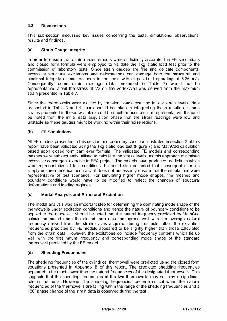
4.3 Discussions This sub-section discusses key issues concerning the tests, simulations, observations, results and findings. (a) Strain Gauge Integrity In order to ensure that strain measurements were sufficiently accurate, the FE simulations and closed form formula were employed to validate the 1kg static load test prior to the commission of laboratory tests. Since strain gauges are fine and delicate components, excessive structural excitations and deformations can damage both the structural and electrical integrity as can be seen in the tests with oil-gas fluid operating at 5.36 m/s. Consequently, some strain readings (data presented in Table 7) would not be representative, albeit the stress at V3 on the VortexWell was derived from the maximum strain presented in Table 7. Since the thermowells were excited by transient loads resulting in low strain levels (data presented in Table 3 and 4), care should be taken in interpreting these results as some strains presented in these two tables could be neither accurate nor representative. It should be noted from the initial data acquisition phase that the strain readings were low and unstable as these gauges might be working within their noise regions. (b) FE Simulations All FE models presented in this section and boundary condition illustrated in section 3 of this report have been validated using the 1kg static load test (Figure 7) and MathCad calculation based upon closed form cantilever formula. The validated FE models and corresponding meshes were subsequently utilised to calculate the stress levels, as this approach minimised excessive convergent exercise in FEA project. The models have produced predictions which were representative of test conditions. It should also be noted that convergent exercise simply ensure numerical accuracy, it does not necessarily ensure that the simulations were representative of test scenarios. For simulating higher mode shapes, the meshes and boundary conditions would have to be modified to reflect the changes of structural deformations and loading regimes. (c) Modal Analysis and Structural Excitation The modal analysis was an important step for determining the dominating mode shape of the thermowells under excitation conditions and hence the nature of boundary conditions to be applied to the models. It should be noted that the natural frequency predicted by MathCad calculation based upon the closed form equation agreed well with the average natural frequency derived from the strain cycles acquired during the tests, albeit the excitation frequencies predicted by FE models appeared to be slightly higher than those calculated from the strain data. However, the excitations do include frequency contents which tie up well with the first natural frequency and corresponding mode shape of the standard thermowell predicted by the FE model. (d) Shedding Frequencies The shedding frequencies of the cylindrical thermowell were predicted using the closed form equations presented in Appendix B of this report. The predicted shedding frequencies appeared to be much lower than the natural frequencies of the designated thermowells. This suggests that the shedding frequencies of the two thermowells may not play a significant role in the tests. However, the shedding frequencies become critical when the natural frequencies of the thermowells are falling within the range of the shedding frequencies and a 180˚ phase change of the strain data is observed during the test.

Page 21 of 29 E1937X12
(e) Preliminary Findings In comparing the FOS contours (Figures 20 and 21), it should be noted that the VortexWell has significantly outperformed the standard thermowell in terms of dynamic performance and mechanical strength. Notwithstanding, due diligence should be exercised in interpreting these analytical results as the standard thermowell was operating behind the wake of the VortexWell. Indeed, the standard thermowell was undergoing some phase changes and in some cases it exhibited a sign of significant dynamic amplification. This indicated that the standard thermowell would be operating within the range of its first natural frequency. It should also be noted that high dynamic amplifications resulting from excitation frequencies would also shorten the fatigue and service life of thermowells. 5 CONCLUSIONS AND RECOMMENDATIONS The results of the work programme have been analysed and presented in this report showing dynamic performance and mechanical strengths of the two designated thermowells. A comparison of dynamic performance and mechanical stresses indicates that the VortexWell has significantly outperformed the standard thermowell in this project.
To verify and hence confirm the findings, it is recommended that:
1. a CFD simulation study be undertaken to verify if unsteady flows and installation effects could affect the dynamic performance and hence impose higher loading magnitude over the two thermowells;
2. further laboratory tests be carried out to individually and independently test the
VortexWell and standard thermowell at NEL’s flow process line;
3. an experimental modal analysis be carried out to verify the natural frequencies of these two thermowells which might be influenced by installation effects and unsteady flows.

Page 22 of 29 E1937X12
REFERENCES
1 Brock J.E., ‘Stress Analysis of Thermowells’ National Technical Information Service, U.S. Department of Commerce, 11 November 1974.
2 Oakes T., ‘Computational Fluid Dynamics Modelling’, CDS Cygnet Development
Services Ltd, Okazaki Report_V3_TO_ApRE_1_300608. 30/06/2008.
3 Murdock J.W., ‘Power Test Code: Thermometer Wells’, Journal Engineering for Power,
1959.
4 Measurement of fluid flow by means of pressure differential devices inserted in circular cross-section conduits running full – Part 1: General principles and requirements. BS EN ISO 5167 – 1:2003, pp 3.
5 Massey, B.S. Mechanics of fluids, 3rd Edition, pp 300.
6 Roark, R.J., and Young, W.C. Formulas for Stress and Strain, Fifth Edition, pp 576.

Page 23 of 29 E1937X12
APPENDIX II
Test Conditions and Data Acquisition Log
TABLE A1
SUMMARY OF TEST PARAMETERS
TABLE A2
FLUID VELOCITIES, FLOW RATES AND REYNOLDS NUMBERS
Fluid velocity – m/s 1.07 2.14 3.22 4.28 5.82
Flow rate – l/s 20 40 60 80 100
Reynolds No. of thermowells 2.65x10³
5.31x10³
8.02x10³
1.07x10⁴
1.35x10⁴
Reynolds No. of 6” sch. 40, process line
2.63x10⁴
5.27x10⁴
7.95x10⁴
1.06x10⁵
1.33x10⁵
The Reynolds number [4] for the 6” process line is given by:
VDD Re (1)
where: ReD is the Reynolds number of the process line; V is the fluid velocity; D is the inner diameter of the pipe section;
is the kinematic viscosity.
Ave.
Temperature
Ave. Absolute
Presssure
Fluid
Density
Fluid Kin.
Viscosity
Fluid Dyn.
Viscosity
Ref. Volume
Flow Rate
°C Pa kg/m³ m²/s Pa.s m³/s
04/04/12 11:44 19.960 247690 820.741 6.2675E-06 5.1440E-03 0.01981
04/04/12 11:52 19.994 251606 820.720 6.2617E-06 5.1391E-03 0.04000
04/04/12 12:01 20.120 259679 820.638 6.2405E-06 5.1212E-03 0.05961
04/04/12 12:11 20.143 259454 820.623 6.2368E-06 5.1181E-03 0.05964
04/04/12 12:18 20.271 271368 820.543 6.2154E-06 5.1000E-03 0.07970
04/04/12 13:54 20.401 275048 820.456 6.1937E-06 5.0817E-03 0.09959
04/04/12 14:46 23.302 319249 818.498 5.7303E-06 4.6902E-03 0.19154
Collection
Date & TimePressure
Page 24 of 29 E1937X12
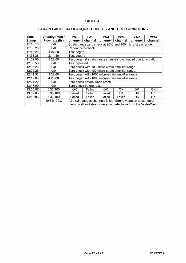
TABLE A3
STRAIN GAUGE DATA ACQUISITION LOG AND TEST CONDITIONS
Time Stamp
Velocity (m/s) / Flow rate (l/s)
TW1 channel
TW2 channel
TW3 channel
VW1 channel
VW2 channel
VW3 channel
11:18:10 0/0 Strain gauge zero check at 20C and 100 micro-strain range.
11:36:26 0/0 Repeat zero check.
11:43:21 1.07/20 Test began.
11:53:38 2.14/40 Test began.
11:02:05 3.22/60 Test began & strain gauge channels overloaded due to vibration.
12:03:58 0/0 Test repeated.
12:08:26 0/0 Zero check with 100 micro-strain amplifier range.
12:09:25 0/0 Zero check with 100 micro-strain amplifier range.
12:11:52 3.22/60 Test began with 1000 micro-strain amplifier range.
12:19:00 4.28/80 Test began with 1000 micro-strain amplifier range.
12:24:22 0/0 Zero check before lunch break.
13:47:09 0/0 Zero check before restart.
13:55:07 5.36/100 OK Failed OK OK OK OK
13:59:03 5.36/100 Failed Failed Failed OK OK OK
14:18:06 5.36/100 Failed Failed Failed Failed OK OK
10.31/192.3 All strain gauges channels failed. Strong vibration at standard thermowell and strains were not detectable from the VortexWell.

Page 25 of 29 E1937X12
APPENDIX III
Prediction of Shedding Frequency The shedding frequency generated by a smooth cylinder is given by:
d
VStf (2)
Alternatively, the empirical formula [5] for calculating the shedding frequency of a cylinder is given by:
)Re
7.191(198.0
d
Vf (3)
where: f is the shedding frequency in Hz; St is Strouhal number; V is flow velocity; d is the diameter of the cylinder;
is kinematic viscosity of the fluid; Re is Reynolds number of the cylinder. Equation 2 is generally valid for the range 250 < Re < 2 x 10⁵. Figure A1 below represents the experimental relationship between Strouhal number and the Reynolds number of the cylinder utilised for the test.
V
fdSt
VdRe
Figure B1 Strouhal Number vs. Reynolds Number
(Experimental Data for Cylinder)

Page 26 of 29 E1937X12
APPENDIX IV
Prediction of Natural Frequency using Closed Form Equations The natural Frequencies of a cylindrical cantilever [6] can be approximated by using the closed form equation illustrated below.
42 Wl
gEI
Knn
(4)
where:
n is the natural frequency of the cantilever beam;
E is the young modulus of the beam; W is the uniformly distributed load along the beam; l is the length of the beam; Kn is a beam constant.
TABLE C1
FUNDAMENTAL MODES AND Kn
Mode number Kn Nodal position/l
1 3.52 0
2 22.00 0, 0.783
3 61.70 0, 0.504, 0.868
4 121.00 0, 0.358, 0.644, 0.905
5 200.00 0, 0.279, 0.500, 0.723, 0.926

Page 27 of 29 E1937X12
APENDIX V
Thermowell CFD
Vorticity Magnitude (1/s)
Turbulence Kinetic Energy (m2/s2)
Velocity Magnitude (m/s)
-600
-400
-200
0
200
400
600
5.4 5.45 5.5 5.55 5.6 5.65
Lift
co
effi
cien
t -
C L
Time (s)
Upstream Thermowell
Downstream Thermowell
Force experienced by each thermowell varying with time

APPENDIX VI

APPENDIX VI