Embed Size (px)
Citation preview

ORNL/TM-2013/430
Evaluation of Ultrasonic Techniques on Concrete Structures
September 2013
Prepared by
Dwight Clayton – ORNL Cyrus Smith – ORNL Christopher C. Ferraro – Lynch and Ferraro Engineering, Inc. Jordan Nelson – Lynch and Ferraro Engineering, Inc. Lev Khazanovich – University of Minnesota Kyle Hoegh – University of Minnesota Satish Chintakunta – Engineering & Software Consultants Inc. John Popovics – University of Illinois – Urbana-Champaign Hajin Choi – University of Illinois – Urbana-Champaign Suyun Ham – University of Illinois – Urbana-Champaign

DOCUMENT AVAILABILITY
Reports produced after January 1, 1996, are generally available free via US Department of Energy (DOE) SciTech Connect. Website http://www.osti.gov/scitech/ Reports produced before January 1, 1996, may be purchased by members of the public from the following source: National Technical Information Service 5285 Port Royal Road Springfield, VA 22161 Telephone 703-605-6000 (1-800-553-6847) TDD 703-487-4639 Fax 703-605-6900 E-mail [email protected] Website http://www.ntis.gov/support/ordernowabout.htm Reports are available to DOE employees, DOE contractors, Energy Technology Data Exchange representatives, and International Nuclear Information System representatives from the following source: Office of Scientific and Technical Information PO Box 62 Oak Ridge, TN 37831 Telephone 865-576-8401 Fax 865-576-5728 E-mail [email protected] Website http://www.osti.gov/contact.html
This report was prepared as an account of work sponsored by an agency of the United States Government. Neither the United States Government nor any agency thereof, nor any of their employees, makes any warranty, express or implied, or assumes any legal liability or responsibility for the accuracy, completeness, or usefulness of any information, apparatus, product, or process disclosed, or represents that its use would not infringe privately owned rights. Reference herein to any specific commercial product, process, or service by trade name, trademark, manufacturer, or otherwise, does not necessarily constitute or imply its endorsement, recommendation, or favoring by the United States Government or any agency thereof. The views and opinions of authors expressed herein do not necessarily state or reflect those of the United States Government or any agency thereof.

ORNL/TM-2013/430
Measurement Science and Systems Engineering Division
EVALUATION OF ULTRASONIC TECHNIQUES ON CONCRETE
STRUCTURES
Dwight Clayton
Cyrus Smith
Chris Ferraro
Jordan Nelson
Lev Khazanovich
Kyle Hoegh
Satish Chintakunta
John Popovics
Hajin Choi
Suyun Ham
Date Published: September 2013
Prepared by
OAK RIDGE NATIONAL LABORATORY
Oak Ridge, Tennessee 37831-6283
managed by
UT-BATTELLE, LLC
for the
U.S. DEPARTMENT OF ENERGY
under contract DE-AC05-00OR22725


iii
CONTENTS
Page
LIST OF FIGURES ...................................................................................................................................... v
LIST OF TABLES ....................................................................................................................................... ix
ACKNOWLEDGEMENTS ......................................................................................................................... xi
EXECUTIVE SUMMARY ....................................................................................................................... xiii
1. INTRODUCTION ................................................................................................................................ 1
2. FY 2013 CONCRETE NDE ACTIVITIES .......................................................................................... 3
3. OVERVIEW ......................................................................................................................................... 5
4. DESCRIPTION OF NDE EVALUATION BLOCKS .......................................................................... 7
4.1 OVERVIEW ............................................................................................................................... 7
4.2 REBAR DETECTION BLOCK – SPECIMEN 2 ....................................................................... 8
4.3 VOID AND FLAW DETECTION BLOCK – SPECIMEN 6 .................................................. 12
4.3.1 Overview ...................................................................................................................... 12
4.3.2 Formwork Construction ............................................................................................... 17
4.3.3 Concrete Placement ..................................................................................................... 19
5. EXPERIMENTAL SETUP AND EQUIPMENT ............................................................................... 23
5.1 OVERVIEW OF EXPERIMENTAL SETUP .......................................................................... 23
5.2 MIRA EQUIPMENT SETUP AND MEASUREMENT TECHNIQUES ................................ 24
5.2.1 Technical Description of the MIRA Equipment .......................................................... 24
5.2.2 MIRA Measurement Technique................................................................................... 28
5.3 ANTARES EQUIPMENT SETUP AND MEASUREMENT TECHNIQUES ........................ 31
5.3.1 ANTARES Overview .................................................................................................. 31
5.3.2 NDE Instruments Used by ANTARES ........................................................................ 32
5.3.3 Applications for Structures and Materials ................................................................... 33
5.3.4 Continued Research ..................................................................................................... 34
5.4 AIR-COUPLED AND SEMI-COUPLED ULTRASONIC EQUIPMENT SETUP AND
MEASUREMENT TECHNIQUES .......................................................................................... 34
5.4.1 Air-Coupled Impact Echo ............................................................................................ 34
5.4.2 Air-Coupled Ultrasonic Surface Wave ........................................................................ 35
5.4.3 Semi-Coupled Ultrasonic Tomography ....................................................................... 36
6. SIGNAL INTERPRETATION/RESULT ........................................................................................... 39
6.1 MIRA VERSION 1 – UNIVERSITY OF MINNESOTA ........................................................ 39
6.1.1 MIRA Version 1 Analysis of Specimen 6 ................................................................... 39
6.1.2 MIRA Version 1 Analysis of Specimen 2 ................................................................... 51
6.2 MIRA VERSION 2 – ENGINEERING & SOFTWARE CONSULTANTS, INC. .................. 55
6.2.1 Concrete Specimen 6 Horizontal Scan ......................................................................... 56
6.2.2 Concrete Specimen 6 Vertical Scan ............................................................................. 56
6.2.3 Concrete Specimen 2 Horizontal Scan ......................................................................... 58
6.2.4 Concrete Specimen 2 Vertical Scan ............................................................................. 61
6.3 GROUND PENETRATING RADAR (GPR) – LYNCH & FERRARO
ENGINEERING, INC. .............................................................................................................. 63
6.3.1 Concrete Specimen 2 ................................................................................................... 63
6.3.2 Concrete Specimen 6 ................................................................................................... 66
iv
6.4 SHEAR WAVE ULTRASOUND DATA – LYNCH & FERRARO ENGINEERING,
INC. ........................................................................................................................................... 67
6.4.1 Concrete Specimen 2 ................................................................................................... 67
6.4.2 Concrete Specimen 6 ................................................................................................... 68
6.5 AIR-COUPLED AND SEMI-COUPLED ULTRASONIC – UNIVERSITY OF
ILLINOIS AT URBANA-CHAMPAIGN ................................................................................ 72
6.5.1 Air-Coupled Impact Echo ............................................................................................ 72
6.5.2 Air-Coupled Ultrasonic Surface Wave ........................................................................ 73
6.5.3 Semi-Coupled Ultrasonic Tomography ....................................................................... 75
7. CONCLUSIONS ................................................................................................................................ 79
7.1 MIRA VERSION 1 – UNIVERSITY OF MINNESOTA ........................................................ 79
7.2 MIRA VERSION 2 – ENGINEERING & SOFTWARE CONSULTANTS, INC. .................. 79
7.3 ULTRASONIC LINEAR ARRAY AND GROUND-PENETRAING RADAR –
LYNCH & FERRARO ENGINEERING, INC. (LFE) ............................................................. 80
7.4 AIR-COUPLED AND SEMI-COUPLED ULTRASONIC – UNIVERSITY OF
ILLINOIS AT URBANA-CHAMPAIGN ................................................................................ 80
7.5 CONSOLIDATED AND OVERALL CONCLUSIONS .......................................................... 81
8. REFERENCES ................................................................................................................................... 83
APPENDIX A. INTERPRETATION AND ANALYSIS OF ULTRASONIC LINEAR ARRAY
SIGNALS.......................................................................................................................................... A-1
APPENDIX B. INTERPRETING ANTARES DATA FILES ................................................................. B-1

v
LIST OF FIGURES
Figure Page
1. Six key R&D projects identified by workshop participants. ................................................................ 3 2. Four milestones of planned FY 2013 concrete NDE activities. ............................................................ 3 3. Four concrete test specimens. ............................................................................................................... 7 4. Orientation and relative location of rebar mats in the rebar detection block [3]. ................................. 8 5. Rebar locations in the A-side (top) and B-side (bottom) of the rebar detection block [3]. ................... 9 6. 3D rendering of the void and flaw detection block ............................................................................. 12 7. Void and flaw detection Detail Sheet 1. ............................................................................................. 13 8. Void and flaw detection Detail Sheet 2. ............................................................................................. 14 9. Void and flaw detection Detail Sheet 3. ............................................................................................. 15 10. Void and flaw detection Detail Sheet 4. ............................................................................................. 16 11. Pervious concrete prisms suspended for the ANTARES void and flaw detection block. .................. 17 12. Three rebar pieces including the two moving specimens in void and flaw detection block. .............. 18 13. Consolidating the specimen with an internal vibrator. ....................................................................... 19 14. Installing the surface level pervious concrete prism. .......................................................................... 20 15. Installing wet-sieved concrete into the surface to realistically simulate poor consolidation. ............. 20 16. ANTARES void and flaw detection block in scanner frame with surface defects visible. ................. 21 17. 4 in. × 4 in. grid pattern on wall surface of Specimen 2 used to position MIRA devices................... 23 18. Defects built into the back side of Specimen 6 ................................................................................... 24 19. Ultrasonic linear array device with illustration ................................................................................... 25 20. Example of impulse time history from a transducer pair .................................................................... 26 21. (a) Front view of MIRA Tomographer; (b) side view of MIRA......................................................... 26 22. Multiple ray paths involved during a test with MIRA. ....................................................................... 27 23. Schematic of MIRA device positioning and mark on the MIRA device to aid in positioning. .......... 28 24. Horizontal scanning procedure. .......................................................................................................... 29 25. Sets and positions used in the horizontal scanning procedure. ........................................................... 30 26. Vertical scanning procedure. .............................................................................................................. 30 27. Sets and positions used in the vertical scanning procedure. ............................................................... 31 28. ANTARES scanner system with a concrete specimen and representative analysis images. .............. 32 29. Various instruments installed on the ANTARES system. .................................................................. 33 30. Illustration of equipment used for air-coupled impact-echo tests. ...................................................... 35 31. Illustration of air-coupled ultrasonic surface wave method ................................................................ 36 32. Illustration of ultrasonic tomography equipment. ............................................................................... 37 33. Illustration of ultrasonic scanning procedure ...................................................................................... 37 34. Schematic of concrete specimen 6. ..................................................................................................... 40 35. Example SAFT-FW scan along with automated layer boundary detection results............................. 41 36. Schematic of wall specimen 6 and MIRA reconstructions ................................................................. 42 37. SAFT 3D reconstruction of reinforcements. ....................................................................................... 42 38. Schematic of concrete specimen 6 and MIRA reconstructions .......................................................... 43 39. Schematic of concrete specimen 6 reconstructions, including locations with gaps at back wall........ 44 40. SAFT panoramic reconstruction in the vertical direction ................................................................... 45 41. SAFT Panoramic reconstruction with a zoomed portion. ................................................................... 45 42. SAFT 3D reconstruction of Specimen 6 ............................................................................................. 46 43. SAFT 3D reconstruction showing shadowing below the top vertical half of R1. .............................. 46 44. Schematic of wall Specimen 6 and MIRA reconstruction. ................................................................. 47 45. Schematic of concrete specimen 6 and individual SAFT-IA reconstructions .................................... 48 46. Use of SAFT-Panoramic and relative reflectivity measures to identify a vertical crack. ................... 49

vi
47. CR2 detection using SAFT Panoramic and relative reflectivity signal interpretation. ....................... 50 48. Specimen 2 dimensions and orientation. ............................................................................................ 51 49. Example portion of Specimen 2 showing various sized reinforcements. ........................................... 52 50. A 3D reconstruction showing the various sized reinforcements. ........................................................ 53 51. SAFT 3D view of the reinforcement relative reflections in relation to the interface. ......................... 54 52. Detection below heavy reinforcement. ............................................................................................... 55 53. (a) Front view of concrete specimen 6; (b) 3D rendering showing the three large rebar
elements running vertically through the middle of the concrete specimen and the
honeycomb on the left side of the concrete specimen (as seen from the front view). ............. 56 54. (a) Front view of specimen 6; (b) top view of specimen 6; (c) 3D rendering shows the
honeycomb, cracks, and the large flaw around rebar 1. .......................................................... 57 55. (a) Stitched B-scan from vertical scan of specimen 6 showing honeycombs and cracks; (b)
stitched B-scan from vertical scan of specimen 6 showing embedded flaw around the
length of rebar 1. ..................................................................................................................... 58 56. (a) Top view of specimen 2; (b) 3D rendering showing the rebar running vertically in the
specimen. ................................................................................................................................. 59 57. (a) Top view of concrete specimen 2; (b) 3D rendering showing the overlying sections of rebar
running vertically in the concrete specimen. ........................................................................... 60 58. (a) Top view of specimen 2; (b) 3D rendering showing the overlying sections of rebar running
vertically in the specimen (c). ................................................................................................. 61 59. (a) Side view of specimen 2; (b) 3D rendering shows the rebar running horizontally in the
concrete specimen close to the top of the slab. ....................................................................... 62 60. (a) Side view of specimen 2; (b) 3D rendering shows the rebar running horizontally in the
concrete specimen close to the bottom of the slab. ................................................................. 63 61. C-scan image of x-oriented GPR scans of rebar detection block side A ............................................ 64 62. C-scan image of y-oriented GPR scans of rebar detection block side A ............................................ 65 63. C-scan image of GPR scan of void and flaw detection block ............................................................. 66 64. GPR line scan showing a weak reflection of the leftmost rebar due to delamination......................... 66 65. C-scan image of ultrasound scan of detection block side A with Hilbert visualization...................... 67 66. Tomographic image of the xz plane of rebar block ............................................................................. 68 67. Initial ultrasound data processing for the void and flaw detection block. .......................................... 69 68. Ultrasound C-scan image with no secondary processing at a depth of 90 mm. .................................. 70 69. Ultrasound C-scan image at a depth of 120 mm ................................................................................. 71 70. Hilbert transform C-scan ultrasound image at 120 mm depth. ........................................................... 71 71. Ultrasound C-scan “shadow” image of the back wall of the void and flaw detection block. ............. 72 72. Impact-echo peak frequency (Hz) scan image for Specimens 2 and 6. .............................................. 73 73. Ultrasonic surface wave amplitude scan image (volts) for Specimens 2 and 6. ................................. 74 74. Ultrasonic surface wave arrival time scan image (seconds) for Specimens 2 and 6. .......................... 74 75. Ultrasonic surface wave arrival time plots using image transparency for Specimen 6 ....................... 75 76. Ultrasonic velocity tomograph slice data for Specimen 6. ................................................................. 76 77. Illustration of procedure to remove ray density artifact indications from thresholded binary
image plots of tomographic data. ............................................................................................ 77 78. Thresholded (25%) binary image plots of tomographic data set for Specimen 6 after removal
of ray path artifacts .................................................................................................................. 77 79. Representation of potential contributing point sources at a constant time (Roundtrip) from the
emitting/receiving transducer according to the fundamental expression. ................................. 4 80. Linear array representation. .................................................................................................................. 5 81. Schematic of the CRCP subsurface at the example scan location. ....................................................... 6 82. Example emitting-receiving pairs from an ultrasonic linear array scan. .............................................. 7 83. Example SAFT reconstruction with the apodization factor equal to (a) 1 and (b). .............................. 8 84. Determination of the direct arrival peak using the instantaneous amplitude envelope. ...................... 10

vii
85. SAFT reconstruction and example column data. ................................................................................ 11 86. SAFT-IA reconstruction and example column data. .......................................................................... 12 87. Forensic verification of the focused reinforcement location within the SAFT-IA B-scan. ................ 12 88. SAFT-IA B-scans from the cored location ......................................................................................... 13 89. Schematic representation of the process of creating SAFT-3D reconstructions. ................................ 14 90. SAFT 3D reconstruction using the SAFT-IA B-scan reconstructions shown in Fig. 88. ................... 14 91. Example set of nine overlapping SAFT-IA B-scans used to create a SAFT panoramic. ................... 16 92. Five SAFT-Pan examples at a PCC joint. ........................................................................................... 17 93. Progression in identifying the centroid of reflections caused by round inclusions. ............................ 18 94. SAFT-Pan reconstruction with imprecise step size input. .................................................................. 20 95. Determination of overlapping regions between the reconstructions ................................................... 21 96. Similarity of overlapping region curves used for placement of SAFT-IA reconstructions. .............. 23 97. Reconstruction of nine overlapping scans over three dowels ............................................................. 24


ix
LIST OF TABLES
Table Page
1 X-oriented rebar locations by bar index [3] ....................................................................................... 10 2 Y-oriented rebar locations by bar index [3] ......................................................................................... 11 3 Feature in Specimen 6 as detected by MIRA ...................................................................................... 39


xi
ACKNOWLEDGEMENTS
The authors at Oak Ridge National Laboratory would like to express our appreciation to our co-authors
and colleagues: Dr. Shane Boone of the Federal Highway Administration’s NDE Validation Center at the
Turner-Fairbank Highway Research Center; the Florida Department of Transportation’s NDE Validation
Facility; Dr. Chris Ferraro and Jordan Nelson of the Department of Civil and Coastal Engineering,
University of Florida – Gainesville; Dr. Lev Khazanovich and Dr. Kyle Hoegh of the Civil Engineering
Department at the University of Minnesota; Satish Chintakunta of Engineering & Software Consultants,
Inc.; and Dr. John Popovics, Hajin Choi, and Suyun Ham of the Civil Engineering Department at the
University of Illinois at Urbana-Champaign.


xiii
EXECUTIVE SUMMARY
Materials issues are a key concern for the existing nuclear reactor fleet as material degradation can
increase maintenance, downtime, and risk. Extending reactor life to 60 years and beyond will likely
increase the reactor’s susceptibility to, and the severity of known forms of degradation. Additionally, new
mechanisms of materials degradation are also possible. The purpose of the U.S. Department of Energy
Office of Nuclear Energy’s Light Water Reactor Sustainability (LWRS) program is to develop
technologies and other solutions that can improve the reliability, sustain the safety, and extend the
operating lifetimes of nuclear power plants (NPPs) beyond 60 years.
A multitude of concrete-based structures are typically part of a light water reactor (LWR) plant,
functioning as the foundation, support, shielding, and containment. Concrete has been used in NPP
construction because of its inexpensiveness, its structural strength, and its ability to shield radiation.
Examples of concrete structures important to LWR safety include the containment building, the spent fuel
pool, and cooling towers. Such use has made its long-term performance crucial for the safe operation of
commercial NPPs.
In concrete structures, age-related degradation may affect engineering properties, structural
resistance/capacity, failure mode, and location of failure initiation, which in turn may affect the ability of
a structure to withstand challenges in service. To ensure the safe operation of NPPs, it is essential that the
effects of potential degradation of the plant structures, as well as systems and components, be assessed
and managed during both the current operating license period as well as subsequent license renewal
periods. In contrast to many mechanical and electrical components, replacing many concrete structures is
impractical. Therefore it is necessary that safety issues related to plant aging and continued service of the
concrete structures be resolved through sound scientific and engineering understanding.
Unlike most metallic materials, reinforced concrete is a nonhomogeneous material; a composite with a
low density matrix, reinforced concrete is a mixture of cement, sand, aggregate and water, and with a high
density reinforcement (typically 5% in NPP containment structures) consisting of steel rebar or tendons.
Plants have been typically built with local cement and aggregate fulfilling the design specifications
regarding strength, workability, and durability, but as a consequence, each plant’s concrete composition is
unique and complex. In addition, NPP concrete structures are often inaccessible, containing large volumes
and massively thick concrete structures that are exposed to different environments (moisture,
temperature) and a diversity of degradation mechanisms (high temperatures, radiation exposure, chemical
reactions) at different plant sites, all of which adds to the complexity of determining the integrity/quality
of the concrete.
The ORNL Concrete NDE efforts are directed toward addressing gaps between available techniques and
the technology needed to perform the measurements identified during the LWRS Nondestructive
Evaluation Workshop held on July 31, 2012, on the current NPP fleet [1]. Several important themes are
the focus of our work:
1. Need to survey available samples
Comparative testing on the various NDE concrete measurement techniques will require concrete
samples with known material properties, voids, internal microstructure flaws, and reinforcement
locations. These samples can be artificially created under laboratory conditions where the various
properties can be controlled. In addition, concrete samples that have been removed from the field and
exposed to known degradation mechanisms (different levels of radiation, temperature, chemical
reaction) provide the most realistic concrete aging specimens.

xiv
2. Techniques to perform volumetric imaging on thick reinforced concrete sections
A technique or a combination of techniques that could reliably and quickly generate an image of the
volume of thick concrete structures will significantly enhance the interpretability of the outcome of
the various NDE measurement methodologies and is greatly desired.
3. Determination of physical and chemical properties as a function of depth
Knowledge of the physical and chemical properties of a concrete structure, especially as a function of
depth, will provide highly relevant information on its structural integrity.
4. Techniques to examine interfaces between concrete and other materials
In some cases, the structural concrete to be inspected is covered by a steel liner. Presently there are no
techniques for inspecting concrete through steel.
5. Development of acceptance criteria – model and validation
Through modeling and validation, an acceptance criterion needs to be developed to determine that a
concrete structure is “good enough.” For each NDE concrete measurement metric (void size, crack
size, reinforcement degradation, physical properties), an upper and lower acceptance boundary needs
to be determined.
6. Need for automated scanning system for any of the NDE concrete measurement systems
Due to the massively large concrete areas to be surveyed, an automated scanning system for any NDE
concrete measurements is greatly desired.
This report is focused on the ORNL efforts toward item #2, techniques to perform volumetric imaging on
thick reinforced concrete sections. ORNL comparatively evaluated a number of ultrasonic techniques on
concrete, using some concrete specimens that had previously been identified in the ORNL report
Summary of Large Concrete Samples, ORNL-TM-2013/223 [2]. Since no concrete specimens truly
representative of the reinforced concrete sections found in NPPs were identified in this report, it was
decided to utilize two 6.5 ft × 5.0 ft × 10 in. concrete test specimens from the Florida Department of
Transportation’s (FDOT’s) NDE Validation Facility in Gainesville, Florida:
1. a rebar detection block (Specimen 2), which is a specimen with various placements of rebar but
without any known flaws, and
2. a void and flaw detection block (Specimen 6), which is an unreinforced specimen with simulated
cracking and nonconsolidation flaws.
ORNL chose to evaluate seven different ultrasonic techniques:
1. Ultrasonic linear array device (Germann Instruments MIRA Tomographer Version 1)
2. Ultrasonic linear array device (Germann Instruments MIRA Tomographer Version 2)
3. Shear wave ultrasonic array (Germann Instruments EyeCon)
4. Ground-penetrating radar (GPR) (GSSI SIR3000 with 2.6 GHz antenna)
5. Air-coupled impact-echo
6. Air-coupled ultrasonic surface wave
7. Semi-coupled ultrasonic
ORNL invited four different organizations to participate in the testing:
1. University of Minnesota – Civil Engineering Department, which utilized the Germann Instruments
MIRA Tomographer Version 1
xv
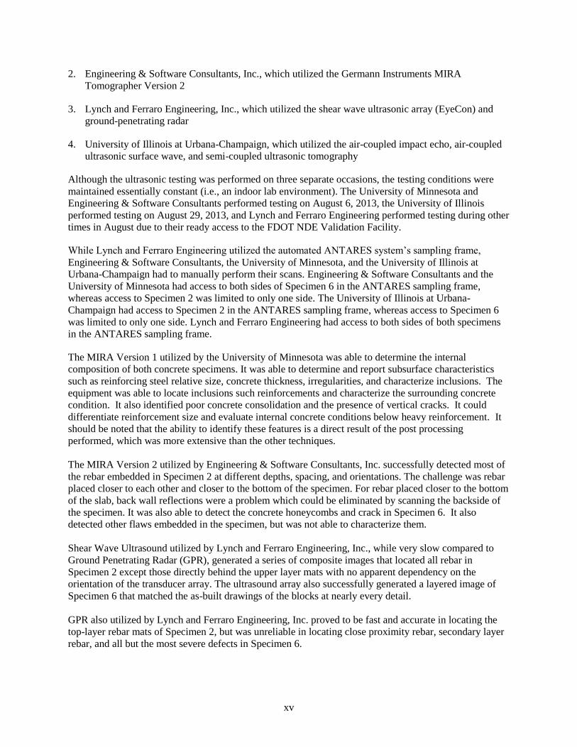
2. Engineering & Software Consultants, Inc., which utilized the Germann Instruments MIRA
Tomographer Version 2
3. Lynch and Ferraro Engineering, Inc., which utilized the shear wave ultrasonic array (EyeCon) and
ground-penetrating radar
4. University of Illinois at Urbana-Champaign, which utilized the air-coupled impact echo, air-coupled
ultrasonic surface wave, and semi-coupled ultrasonic tomography
Although the ultrasonic testing was performed on three separate occasions, the testing conditions were
maintained essentially constant (i.e., an indoor lab environment). The University of Minnesota and
Engineering & Software Consultants performed testing on August 6, 2013, the University of Illinois
performed testing on August 29, 2013, and Lynch and Ferraro Engineering performed testing during other
times in August due to their ready access to the FDOT NDE Validation Facility.
While Lynch and Ferraro Engineering utilized the automated ANTARES system’s sampling frame,
Engineering & Software Consultants, the University of Minnesota, and the University of Illinois at
Urbana-Champaign had to manually perform their scans. Engineering & Software Consultants and the
University of Minnesota had access to both sides of Specimen 6 in the ANTARES sampling frame,
whereas access to Specimen 2 was limited to only one side. The University of Illinois at Urbana-
Champaign had access to Specimen 2 in the ANTARES sampling frame, whereas access to Specimen 6
was limited to only one side. Lynch and Ferraro Engineering had access to both sides of both specimens
in the ANTARES sampling frame.
The MIRA Version 1 utilized by the University of Minnesota was able to determine the internal
composition of both concrete specimens. It was able to determine and report subsurface characteristics
such as reinforcing steel relative size, concrete thickness, irregularities, and characterize inclusions. The
equipment was able to locate inclusions such reinforcements and characterize the surrounding concrete
condition. It also identified poor concrete consolidation and the presence of vertical cracks. It could
differentiate reinforcement size and evaluate internal concrete conditions below heavy reinforcement. It
should be noted that the ability to identify these features is a direct result of the post processing
performed, which was more extensive than the other techniques.
The MIRA Version 2 utilized by Engineering & Software Consultants, Inc. successfully detected most of
the rebar embedded in Specimen 2 at different depths, spacing, and orientations. The challenge was rebar
placed closer to each other and closer to the bottom of the specimen. For rebar placed closer to the bottom
of the slab, back wall reflections were a problem which could be eliminated by scanning the backside of
the specimen. It was also able to detect the concrete honeycombs and crack in Specimen 6. It also
detected other flaws embedded in the specimen, but was not able to characterize them.
Shear Wave Ultrasound utilized by Lynch and Ferraro Engineering, Inc., while very slow compared to
Ground Penetrating Radar (GPR), generated a series of composite images that located all rebar in
Specimen 2 except those directly behind the upper layer mats with no apparent dependency on the
orientation of the transducer array. The ultrasound array also successfully generated a layered image of
Specimen 6 that matched the as-built drawings of the blocks at nearly every detail.
GPR also utilized by Lynch and Ferraro Engineering, Inc. proved to be fast and accurate in locating the
top-layer rebar mats of Specimen 2, but was unreliable in locating close proximity rebar, secondary layer
rebar, and all but the most severe defects in Specimen 6.

xvi
Air-Coupled Impact Echo and Ultrasonic Surface Wave imaging tests utilized by the University of Illinois
at Urbana-Champaign were carried out on both samples. Semi-Coupled Ultrasonic Through Thickness
Tomography also utilized by the University of Illinois was carried out on only Specimen 6. As expected
based on the physics of these techniques, none of these Nondestructive Evaluation (NDE) test methods
were able to detect the presence of well-bonded embedded steel bar in either specimen. However, each of
the tests did reveal the presence of the embedded voided sections in Specimen 6, and the Semi-Coupled
Ultrasonic Through Thickness Tomography appeared to indicate locations of unbonded steel bar. By
analyzing the results of all test methods together, the locations of the defected regions within Specimen 6
could be ascertained with reasonable accuracy.
Overall, all seven of these techniques performed well on the two selected test specimens even though
each method has some limitations and shortcomings. Each technique has situations where it performs
very well and other situations where it is somewhat lacking in performance. While the individual merits
or shortcomings of each technique could be discussed, that is not the goal of this research. The goal is to
provide a baseline performance indication of each technique. It is clear from these results that
improvements in volumetric imaging can be made through research in advanced processing techniques
and that some or all of these techniques should be tested using a thick concrete specimen representative of
NPP structures. Of course, the ultimate solution to volumetric imaging of a thick concrete section might
be a fusion of data from various technologies.

1
1. INTRODUCTION
A multitude of concrete-based structures are typically part of a light water reactor (LWR) plant,
functioning as foundation, support, shielding, and containment. Concrete has been used in the
construction of nuclear power plants (NPPs) because of its inexpensiveness, its structural strength, and its
ability to shield radiation. Examples of concrete structures important to LWR safety include the
containment building, the spent fuel pool, and cooling towers. Such use has made its long-term
performance crucial for the safe operation of commercial NPPs.
Extending reactor life to 60 years and beyond will likely increase the reactor’s susceptibility to, and the
severity of known forms of degradation. Additionally, new mechanisms of materials degradation are also
possible. Unlike most metallic materials, reinforced concrete is a nonhomogeneous material; a composite
with a low-density matrix, reinforced concrete is a mixture of cement, sand, aggregate, and water, and
with a high-density reinforcement (typically 5% in NPP containment structures) consisting of steel rebar
or tendons. Plants have been typically built with local cement and aggregate fulfilling the design
specification regarding strength, workability, and durability; as a consequence, each plant’s concrete
composition is unique and complex. NPP concrete structures are also often inaccessible and contain large
volumes of massively thick concrete. These structures are exposed to different environments (moisture,
temperature) and a diversity of degradation mechanisms (high temperatures, radiation exposure, and
chemical reactions) at different plant sites, all of which add to the complexity of determining the
integrity/quality of the concrete.
With respect to the concrete structures in NPPs, age-related degradation may affect engineering
properties, structural resistance/capacity, failure mode, and locations of failure initiation that in turn may
affect the ability of a structure to withstand challenges in service. In contrast to many mechanical and
electrical components, replacement of many concrete structures is currently considered impractical.
Therefore, it is necessary that safety issues related to concrete structures and plant aging are resolved
through sound scientific and engineering understanding.
To assist in the identification and evaluation of the needed research and development (R&D), a Light
Water Reactor Sustainability (LWRS) Concrete Nondestructive Evaluation (NDE) workshop was held at
Oak Ridge National Laboratory (ORNL) on July 31, 2012, to address gaps between available concrete
NDE techniques and the technology needed to make quantitative measurements to determine the
durability and performance of concrete structures in our current NPP fleet. Expert participants were
identified from a variety of disciplines as well as an assortment of institutions. The represented
institutions included the Electrical Power Research Institute (EPRI), the US Nuclear Regulatory
Commission (NRC), Electricité de France, the Swiss Association for Technical Inspection, Department of
Energy (DOE) National Laboratories, various universities, and industry representatives.
While the workshop participants identified many potential and worthwhile R&D projects related to
concrete NDE, six key technology gaps were identified as being the highest priority [1]:
1. Need to survey available specimens
Comparative testing on the various NDE concrete measurement techniques will require concrete
specimens with known material properties, voids, internal microstructure flaws, and reinforcement
locations. These specimens can be artificially created under laboratory conditions where the various
properties can be controlled. In addition, concrete specimens that have been removed from the field
and exposed to known degradation mechanisms (different levels of radiation, temperature, chemical
reaction) provide the most realistic concrete aging specimens.

2
2. Techniques to perform volumetric imaging on thick reinforced concrete sections
A technique or a combination of techniques that could reliably and quickly generate an image of the
volume of thick concrete structures will significantly enhance the interpretability of the outcome of
the various NDE measurement methodologies and is greatly desired.
3. Determination of physical and chemical properties as a function of depth
Knowledge of the physical and chemical properties of a concrete structure, especially as a function of
depth, will provide highly relevant information on its structural integrity.
4. Techniques to examine interfaces between concrete and other materials
In some cases, the structural concrete to be inspected is covered by a steel liner. Presently there are no
techniques for inspecting concrete through steel.
5. Development of acceptance criteria – model and validation
Through modeling and validation, an acceptance criterion needs to be developed to determine that a
concrete structure is “good enough.” For each NDE concrete measurement metric (void size, crack
size, reinforcement degradation, physical properties), an upper and lower acceptance boundary needs
to be determined.
6. Need for automated scanning system for any concrete NDE measurement system
Due to the massively large concrete areas to be surveyed, an automated scanning system for any NDE
concrete measurements is greatly desired.
These six key R&D projects were further prioritized and arranged on the basis of the maturity of the
technology required to resolve the gap, the expected impact/importance, and likelihood of completing the
projects within a meaningful timeframe. Availability of funding and resources was not used as a
consideration for determining relative priority.

3
2. FY 2013 CONCRETE NDE ACTIVITIES
As shown in Fig. 1, two projects were selected as the highest priority with proposed starts in FY 2013:
(1) survey of available specimens and (2) volumetric imaging of thick sections. While the proposed
schedule in Fig. 2 assumed slightly over $1 million in FY 2013 for these two tasks, significantly less
funding is actually available. The original tasks associated with these projects have been rescoped and
manipulated; that is, some tasks were shifted to later years to accommodate current funding levels while
still making progress toward the goals identified by the workshop participants. Specifically, the
volumetric imaging of thick sections was limited in scope to investigating primarily ultrasonic methods in
FY 2013. The planned R&D activities for FY 2013 are illustrated in Fig. 2.
Fig. 1. Six key R&D projects identified by workshop participants.
Fig. 2. Four milestones of planned FY 2013 concrete NDE activities.
This ORNL technical memorandum represents the deliverable associated with ID #14, “ORNL Technical
Report on Results of Ultrasonic Techniques.”


5
3. OVERVIEW
ORNL comparatively evaluated a number of ultrasonic techniques on concrete, using some concrete
specimens previously identified in the ORNL report Summary of Large Concrete Samples,
ORNL/TM-2013/223 [2]. Since no concrete specimens identified in this report are truly representative of
the reinforced concrete sections found in NPPs, it was decided to utilize two 6.5 ft × 5.0 ft × 10 in.
concrete test specimens from the Florida Department of Transportation’s (FDOT’s) NDE Validation
Facility in Gainesville, Florida:
(1) the rebar detection block (Specimen 2), which is a specimen with various placements of rebar but
without any known flaws, and
(2) the void and flaw detection block (Specimen 6), which is an unreinforced specimen with simulated
cracking and nonconsolidation flaws.
ORNL chose to evaluate a variety of ultrasonic instrumentation:
1. Ultrasonic linear array device (Germann Instruments MIRA Tomographer Version 1) – The MIRA
Tomographer is an instrument for creating a three-dimensional (3D) representation of internal defects
that may be present in a concrete element. It is based on the ultrasonic pitch–catch method and uses
an antenna composed of an array of dry point contact (DPC) transducers that emit shear waves into
the concrete. The 4 × 10 transducer array is under computer control, and the recorded data are stored
in real time. In non-real time, a computer takes the raw data and creates a 3D image of the reflecting
interfaces within the concrete element.
2. Ultrasonic linear array device (Germann Instruments MIRA Tomographer Version 2) – The MIRA
Tomographer is a state-of-the-art instrument for creating a 3D representation of internal defects that
may be present in a concrete element. It is based on the ultrasonic pitch–catch method and uses an
antenna composed of a 4 × 12 array of DPC transducers that emit shear waves into the concrete. The
transducer array is under computer control, and the recorded data are transferred wirelessly to a host
computer in real time. The computer takes the raw data and creates a 3D image of the reflecting
interfaces with the element for immediate display.
3. Shear wave ultrasonic array (Germann Instruments EyeCon) – EyeConTM
is a portable hand-held
instrument for flaw detection and thickness measurements. It is based on the ultrasonic pitch–catch
method and uses an antenna composed of a 4 × 6 array of DPC transducers that emit shear waves into
the concrete. Test results can be displayed as individual A-scans (reflection amplitude versus time or
depth) or a B-scan (cross section of the test object along a scan line).
4. Ground-penetrating radar (GPR) (GSSI SIR3000 with 2.6 GHz antenna) – GPR uses radar pulses in
the microwave band to image below the surface of a variety of media. It uses reflected signals from
subsurface structures to image, for example, embedded objects, changes in material, voids, and
cracks. The depth of GPR is limited by the electrical conductivity of the material, the transmitted
center frequency, and the radiationed power. Usually, GPR antennas are in contact with the material
for the strongest signal strength.
5. Air-coupled impact-echo – The impact-echo method is a local vibration technique and is able to
obtain information on the depth of the internal reflecting interface. A short duration stress pulse is
introduced into the material to set up a local resonance. When the P-wave reaches the back side of the
material, it is reflected and travels back to the surface where the impact was generated. A sensitive
6
transducer next to the impact point picks up the multiple arrivals of the P-wave from which the
thickness of the material or depth of flaw is calculated.
6. Air-coupled ultrasonic surface wave – Air-coupled ultrasonic testing is a noncontact technique for
nondestructive testing. This technique has been shown to be efficient for the testing of large areas.
The large difference between the impedances of air and the material tends to reduce the efficiency of
the transmitter and receiver, thus hampering the effectiveness of the technique. Development of an
air-couple ultrasonic testing technique is an “up-and-coming” technology.
7. Semi-coupled ultrasonic tomography – In semi-coupled ultrasonic tomography, an electrostatic air-
coupled transducer emits an ultrasonic pulse. The emitted wave pulse is directed at the concrete
surface normal to the surface, initiating a P-wave that propagates into the thickness of the specimen.
The propagating P-wave pulse is detected by an array of accelerometers. The time signal is analyzed
to determine a P-wave arrival time, which is then utilized to form a tomographic P-wave velocity
reconstruction.
ORNL invited four organizations to participate in the testing:
1. University of Minnesota – Civil Engineering Department, which utilized the Germann Instruments
MIRATM
Tomographer Version 1
2. Engineering & Software Consultants, Inc., which utilized the Germann Instruments MIRA
Tomographer Version 2
3. Lynch and Ferraro Engineering, Inc., which utilized the shear wave ultrasonic array (EyeCon) and
ground-penetrating radar, and the Automated Nondestructive Testing for Applied Research and
Evaluation of Structures (ANTARES).
4. University of Illinois at Urbana-Champaign, which utilized the air-coupled impact echo, air-coupled
ultrasonic surface wave, and semi-coupled ultrasonic tomography
Lynch and Ferraro Engineering, Inc., along with the FDOT NDE Validation Facility, provided the two
concrete specimens.
This report describes in Section 4 the details of the construction and makeup of the two concrete
specimens used for testing. Section 5 describes the equipment utilized by each of the four organizations in
their testing. Section 6 presents the results of the ultrasonic testing from each organization, and Section 7
presents the conclusions of the testing.

7
4. DESCRIPTION OF NDE EVALUATION BLOCKS
4.1 OVERVIEW
Lynch and Ferraro Engineering, Inc., along with the FDOT NDE Validation Facility, fabricated six
unique validation blocks for possible use in evaluating the capabilities of instruments for reinforcing steel
detection, elastic property estimation, post-tensioning duct investigation, internal void detection, and
surface flaw evaluation. The six validation blocks, four of which are shown in Fig. 3, are
1. control block (monolithic concrete),
2. rebar detection block,
3. internal post-tensioning (PT) duct block (galvanized steel ducts),
4. slab thickness block,
5. asymmetric internal PT duct block (polypropylene ducts), and
6. void and flaw detection block.
Fig. 3. Four concrete test specimens. Clockwise from top left: rebar detection, steel post tensioning duct
evaluation, polypropylene post tensioning duct evaluation, and slab thickness evaluation blocks in varying
stages of design and construction.

8
From these six specimens, ORNL choose Specimen 2 and Specimen 6 for use in this evaluation since
Specimen 2 was the most heavily reinforced with rebar and Specimen 6 represented several visible and
hidden “defects” typical of aging concrete structures.
4.2 REBAR DETECTION BLOCK – SPECIMEN 2
The rebar detection block was designed to evaluate the effectiveness of NDE instruments in locating rebar
of various diameters, varying depths, and differing proximities to each other. The overall complexity of
the rebar mats makes the design of the block difficult to visualize, but the rebar mats can be described as
two separate layers with each layer having an x-axis and y-axis oriented group of individual bars as shown
in Fig. 4 and Fig. 5 along with Table 1and Table 2.
Fig. 4. Orientation and relative location of rebar mats in the rebar detection block [3].

9
Fig. 5. Rebar locations in the A-side (top) and B-side (bottom) of the rebar detection block [3].

10
Table 1. X-oriented rebar locations by bar index [3]
11
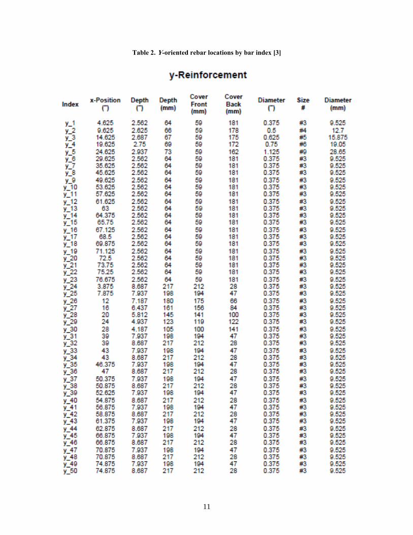
Table 2. Y-oriented rebar locations by bar index [3]
12
4.3 VOID AND FLAW DETECTION BLOCK – SPECIMEN 6
4.3.1 Overview
One of the most common applications for NDE methods in the construction industry is in evaluating the
quality of consolidation in a completed concrete structure. Movement of rebar after initial set, over/under
vibration, mix segregation, and development of bleed water pockets can all lead to entrapped voids within
a concrete structure and compromise its structural integrity. For these reasons, a NDE evaluation block
was fabricated that contains forced honeycombing, delamination, and entrapped air around rebar, and
simulated cracking.
The void and flaw detection block (Specimen 6) was designed to fit in the FDOT NDE Validation
Facility’s standard reusable horizontal block mold. The block contains three pieces of #6 rebar; one with
plastic tubing affixed to simulate entrapped air, one that was moved horizontally in the mold (x-axis) after
initial set of the concrete, and one that was moved vertically in the mold (z-axis) after initial set. The three
rebar lengths are located in the middle third of the block, while on both ends forced honeycombing and
cracking were put in place. On one end section of the block, three prisms of pervious concrete were
suspended along the central plane of the block. The other end has an additional prism of pervious concrete
placed at surface level during concrete placement along with two simulated angled cracks. A schematic of
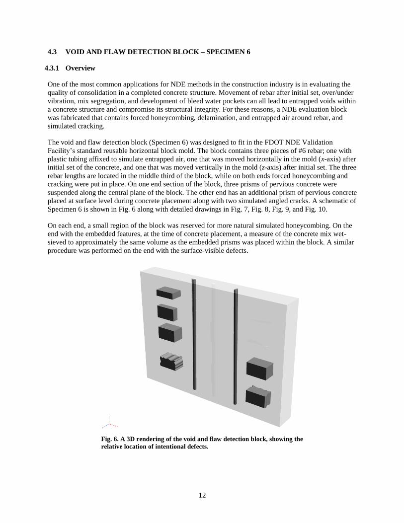
Specimen 6 is shown in Fig. 6 along with detailed drawings in Fig. 7, Fig. 8, Fig. 9, and Fig. 10.
On each end, a small region of the block was reserved for more natural simulated honeycombing. On the
end with the embedded features, at the time of concrete placement, a measure of the concrete mix wet-
sieved to approximately the same volume as the embedded prisms was placed within the block. A similar
procedure was performed on the end with the surface-visible defects.
Fig. 6. A 3D rendering of the void and flaw detection block, showing the
relative location of intentional defects.

13
Fig. 7. Void and flaw detection Detail Sheet 1.

14
Fig. 8. Void and flaw detection Detail Sheet 2.

15
Fig. 9. Void and flaw detection Detail Sheet 3.

16
Fig. 10. Void and flaw detection Detail Sheet 4.

17
4.3.2 Formwork Construction
The first phase of fabricating the void and flaw detection block involved fabricating the prisms of
pervious concrete used to simulate internal and surface level honeycombing, a common symptom of poor
consolidation practices. The prismatic, artificial shape was chosen since its location and volume could be
well defined and documented before NDE analyses were performed.
Two prisms measuring 152 × 152 × 254 mm (6 × 6 × 10 in.) and two prisms measuring 76 × 152 ×
254 mm (3 × 6 × 10 in.) were fabricated by compacting a pervious concrete mixture into a standard
concrete beam specimen mold. The pervious concrete mixture was fabricated in the laboratory following
the mix design submitted to the local concrete plant for delivery; however, the fine aggregate and a
portion of the cement were removed from the mix to reduce the overall paste quantity and approximate a
poorly consolidated region of the delivered mix.
Once the pervious prisms set, they were demolded and saw-cut to length with a wet diamond saw. The
prisms to be installed within the finished block were suspended from fiberglass rods designed to support
the prisms’ weight during formwork construction but, more importantly, designed to hold the prisms
down against buoyant force and laterally in place during concrete placement as shown in Fig. 11. The
fiberglass rods were chosen to be small enough and similar enough in density so as not to appear on
ultrasound scans and were nonmetallic so as not to reflect radar waves.
Fig. 11. Pervious concrete prisms suspended along the middle plane of the formwork for
the ANTARES void and flaw detection block.
The remaining pervious concrete prism was set aside until the date of fabrication, along with two
triangular plates that would be used to form the surface-visible simulated cracks on the other end of the
block.
18
Each triangular plate was used to form a 254 mm (10 in.) long crack of linearly varying depth from 0 to
76.2 mm (3 in.). The plates were set into a small slot cut into a piece of lumber and epoxied in place to
make installation and removal easier.
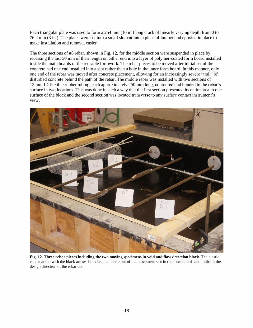
The three sections of #6 rebar, shown in Fig. 12, for the middle section were suspended in place by
recessing the last 50 mm of their length on either end into a layer of polymer-coated form board installed
inside the main boards of the reusable formwork. The rebar pieces to be moved after initial set of the
concrete had one end installed into a slot rather than a hole in the inner form board. In this manner, only
one end of the rebar was moved after concrete placement, allowing for an increasingly severe “trail” of
disturbed concrete behind the path of the rebar. The middle rebar was installed with two sections of
12 mm ID flexible rubber tubing, each approximately 250 mm long, contoured and bonded to the rebar’s
surface in two locations. This was done in such a way that the first section presented its entire area to one
surface of the block and the second section was located transverse to any surface contact instrument’s
view.
Fig. 12. Three rebar pieces including the two moving specimens in void and flaw detection block. The plastic
caps marked with the black arrows both keep concrete out of the movement slot in the form boards and indicate the
design direction of the rebar end.
19
4.3.3 Concrete Placement
After the formwork was completed, concrete was ordered from a local ready-mix plant. The mix was
designed for structural strength, with an approximate compressive strength of 4000 psi, but included
enough retarding admixture to allow enough working time to install the surface defects. Concrete was
carefully placed around the embedded pervious concrete prisms and, once level with the top of the large
prism, a volume of concrete equal to the large prism was wet-sieved through a No. 4 sieve and placed by
hand immediately below the fabricated pervious concrete prisms. This area represented a more realistic
but more geometrically difficult-to-define area of internal honeycombing. A similar procedure was
performed with the surface-visible defects during their installation.
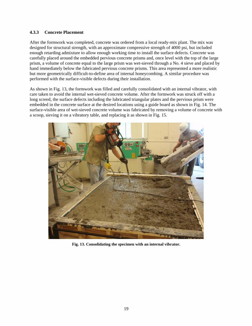
As shown in Fig. 13, the formwork was filled and carefully consolidated with an internal vibrator, with
care taken to avoid the internal wet-sieved concrete volume. After the formwork was struck off with a
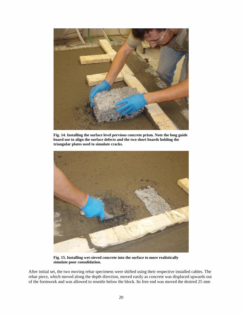
long screed, the surface defects including the lubricated triangular plates and the pervious prism were
embedded in the concrete surface at the desired locations using a guide board as shown in Fig. 14. The
surface-visible area of wet-sieved concrete volume was fabricated by removing a volume of concrete with
a scoop, sieving it on a vibratory table, and replacing it as shown in Fig. 15.
Fig. 13. Consolidating the specimen with an internal vibrator.
20
Fig. 14. Installing the surface level pervious concrete prism. Note the long guide
board use to align the surface defects and the two short boards holding the
triangular plates used to simulate cracks.
Fig. 15. Installing wet-sieved concrete into the surface to more realistically
simulate poor consolidation.
After initial set, the two moving rebar specimens were shifted using their respective installed cables. The
rebar piece, which moved along the depth direction, moved easily as concrete was displaced upwards out
of the formwork and was allowed to resettle below the block. Its free end was moved the desired 25 mm
21
per design. The laterally moving rebar specimen had a more complicated cable system guided through a
lubricated tube into the formwork itself. This system failed to move the rebar as desired, and it was
confirmed after measurement that this rebar piece moved only 8 mm.
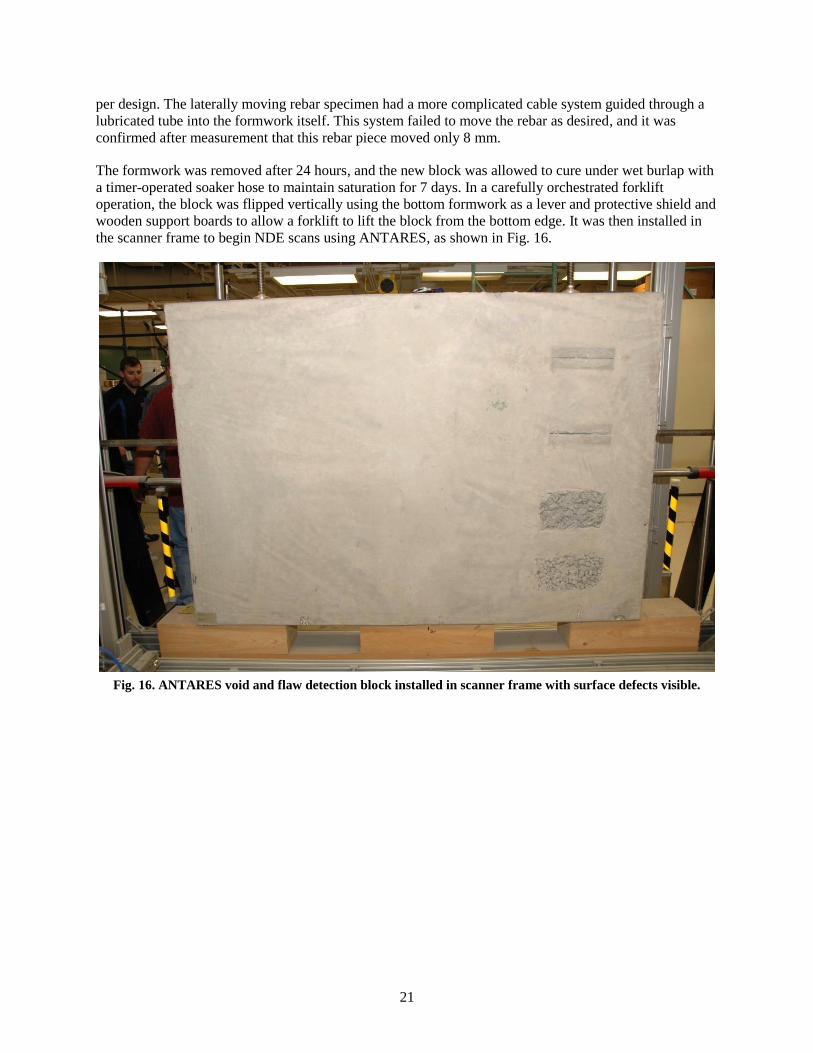
The formwork was removed after 24 hours, and the new block was allowed to cure under wet burlap with
a timer-operated soaker hose to maintain saturation for 7 days. In a carefully orchestrated forklift
operation, the block was flipped vertically using the bottom formwork as a lever and protective shield and
wooden support boards to allow a forklift to lift the block from the bottom edge. It was then installed in
the scanner frame to begin NDE scans using ANTARES, as shown in Fig. 16.
Fig. 16. ANTARES void and flaw detection block installed in scanner frame with surface defects visible.


23
5. EXPERIMENTAL SETUP AND EQUIPMENT
5.1 OVERVIEW OF EXPERIMENTAL SETUP
Although the ultrasonic testing was performed on three separate occasions, the testing conditions were
maintained essentially constant, i.e. an indoor lab environment. The University of Minnesota and
Engineering & Software Consultants performed testing on August 6, 2013. The University of Illinois
performed testing on August 29, 2013, and Lynch and Ferraro Engineering performed testing during other
times in August 2013 since they have ready access to the FDOT NDE Validation Facility.
While Lynch and Ferraro Engineering utilized the automated ANTARES system’s sampling frame,
Engineering & Software Consultants and the University of Minnesota manually performed their scans. The
University of Illinois at Urbana-Champaign utilized a portable scanning frame fabricated at their facility.
Engineering & Software Consultants and the University of Minnesota had access to both sides of Specimen 6
in the ANTARES sampling frame, whereas access to Specimen 2 was limited to only one side. The University
of Illinois at Urbana-Champaign had access to Specimen 2 in the ANTARES sampling frame, providing
access to both sides. While the University of Illinois at Urbana-Champaign had access to both sides of
Specimen 6, access to one side of Specimen 6 was constrained. Lynch and Ferraro Engineering had access to
both sides of both specimens in the ANTARES sampling frame.
For everyone except Lynch and Ferraro, the testing was only conducted on one side of the specimen to
simulate realistic conditions for typical testing arrangements. To allow for comparison of the MIRA
results with other techniques and as-designed internal conditions, a 4 in. × 4in. grid was marked on the
specimen, as shown in Fig. 17. It can be observed in Fig. 18 that the visible defects for Specimen 6 were
all placed on one side of the wall; this side is referred to as the “back wall.” Testing was conducted on the
wall face without defects at the surface (the front side) to determine if the internal inclusions and defects
can be detected without access through the wall. The poor consolidation and cracks that can be observed
on the back side of Specimen 6 are referred to as PC1, PC2, CR1, and CR2, respectively (see Fig. 18).
Fig. 17. A 4 in. × 4 in. grid pattern marked on the wall surface of
Specimen 2 used to position the MIRA devices for Engineering &
Software Consultants and the University of Minnesota.
56”
0”
80”0” Horizontal Position
Ver
tica
l Po
siti
on

24
Fig. 18. Defects built into the back side of Specimen 6 such as cracks
and areas of improperly consolidated concrete.
5.2 MIRA EQUIPMENT SETUP AND MEASUREMENT TECHNIQUES
5.2.1 Technical Description of the MIRA Equipment
The ultrasonic linear array device, MIRA, is an emerging technology for nondestructive diagnostics of the
as-built condition of reinforced concrete structures, especially when specific signal processing and
analysis procedures are developed for the application of interest. This technology is based on the “pitch–
catch” method of sending and receiving shear wave impulses at the surface, requiring only one-sided
access.
Two different versions of the MIRA equipment were used to make the ultrasonic measurements on the
test specimens: (1) MIRA Version 1, used by the University of Minnesota, and (2) MIRA Version 2, used
by Engineering & Software Consultants. The two versions differ in the number of transducer elements
that are used; Version 1 has 40 transducers arranged in a 4 × 10 array, and Version 2 has 48 transducers
arranged in a 4 × 12 array. Additionally, Version 1 software requires that the raw data be collected by the
MIRA and then transferred to an off-board computer for processing, while Version 2 has a self-contained
computer that performs the processing and displays a visual result in near-real time.
Improvements in transducer coupling technology have increased productivity by eliminating the need for
application of a coupling agent to transfer the vibration to the concrete. The DPC transducers have been
developed to transmit and receive shear wave impulses, which allows for measurement pairs with
multiple angles of transmission and reception at reduced transducer spacing for high precision shear wave
impulse measurements and eliminates the need for a manual mechanical impact. The redundancy and
spatial diversity of the measurements provides an opportunity to use the Kirchoff migration-based
focusing to create cross sections of the subsurface structure that correlate to the physical location of the
internal concrete structure. MIRA Version 1consists of a linear array composed of 40 ultrasonic sending
and receiving transducers arranged in 10 channels of four transducers, as can be observed in Fig. 19.
56”
0”
0”80” Horizontal Position
Ver
tica
l Po
siti
on
PC1
PC2
CR1
CR2
25
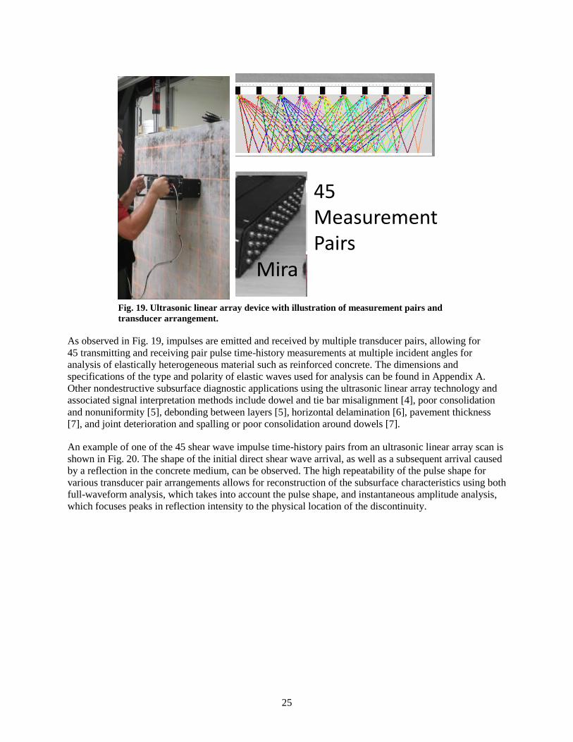
Fig. 19. Ultrasonic linear array device with illustration of measurement pairs and
transducer arrangement.
As observed in Fig. 19, impulses are emitted and received by multiple transducer pairs, allowing for
45 transmitting and receiving pair pulse time-history measurements at multiple incident angles for
analysis of elastically heterogeneous material such as reinforced concrete. The dimensions and
specifications of the type and polarity of elastic waves used for analysis can be found in Appendix A.
Other nondestructive subsurface diagnostic applications using the ultrasonic linear array technology and
associated signal interpretation methods include dowel and tie bar misalignment [4], poor consolidation
and nonuniformity [5], debonding between layers [5], horizontal delamination [6], pavement thickness
[7], and joint deterioration and spalling or poor consolidation around dowels [7].
An example of one of the 45 shear wave impulse time-history pairs from an ultrasonic linear array scan is
shown in Fig. 20. The shape of the initial direct shear wave arrival, as well as a subsequent arrival caused
by a reflection in the concrete medium, can be observed. The high repeatability of the pulse shape for
various transducer pair arrangements allows for reconstruction of the subsurface characteristics using both
full-waveform analysis, which takes into account the pulse shape, and instantaneous amplitude analysis,
which focuses peaks in reflection intensity to the physical location of the discontinuity.
Mira 55 pairs per measurement
1 pair per measurement
Impact Echo
45 Measurement Pairs
Mira 55 pairs per measurement
1 pair per measurement
Impact Echo

26
Fig. 20. Example of impulse time history from a transducer pair
from emitting channel 4 to receiving channel 9 (200 mm spacing).
5.2.1.1 Description of MIRA device
The MIRA Tomographer is intended for inspection of plain concrete and reinforced concrete structural
elements for the purpose of locating voids, foreign inclusions, reinforcement, delaminations, cracks, and
other anomalies with acoustical properties that are different from the surrounding concrete. The device is
designed for the inspection of concrete elements with access to only one side. It can also be used to
measure member thickness.
The MIRA Tomographer is in the form of a prismatic box with two handles [Fig. 21(a)]. The box consists
of an array of shear-wave transducers [Fig. 21(b)], a computer to control the antenna and analyze the
acquired data, a bright LCD display, and keypads for making menu selections. Each handle includes a
“trigger” button to initiate data acquisition at a test location.
Fig. 21. (a) Front view of MIRA Tomographer; (b) side view of MIRA.
-60
-40
-20
0
20
40
60
0 100 200 300 400 500 600
Inte
nsi
ty,
dB
Time, us
200 mm Spacing
4to9
Reflected Pulse
Direct Arrival Pulses
Direct Arrival Pulses
(a)
(b)
27
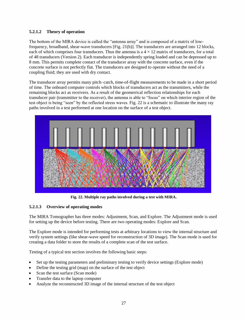
5.2.1.2 Theory of operation
The bottom of the MIRA device is called the “antenna array” and is composed of a matrix of low-
frequency, broadband, shear-wave transducers [Fig. 21(b)]. The transducers are arranged into 12 blocks,
each of which comprises four transducers. Thus the antenna is a 4 × 12 matrix of transducers, for a total
of 48 transducers (Version 2). Each transducer is independently spring loaded and can be depressed up to
8 mm. This permits complete contact of the transducer array with the concrete surface, even if the
concrete surface is not perfectly flat. The transducers are designed to operate without the need of a
coupling fluid; they are used with dry contact.
The transducer array permits many pitch–catch, time-of-flight measurements to be made in a short period
of time. The onboard computer controls which blocks of transducers act as the transmitters, while the
remaining blocks act as receivers. As a result of the geometrical reflection relationships for each
transducer pair (transmitter to the receiver), the antenna is able to “focus” on which interior region of the
test object is being “seen” by the reflected stress waves. Fig. 22 is a schematic to illustrate the many ray
paths involved in a test performed at one location on the surface of a test object.
Fig. 22. Multiple ray paths involved during a test with MIRA.
5.2.1.3 Overview of operating modes
The MIRA Tomographer has three modes: Adjustment, Scan, and Explore. The Adjustment mode is used
for setting up the device before testing. There are two operating modes: Explore and Scan.
The Explore mode is intended for performing tests at arbitrary locations to view the internal structure and
verify system settings (like shear-wave speed for reconstruction of 3D image). The Scan mode is used for
creating a data folder to store the results of a complete scan of the test surface.
Testing of a typical test section involves the following basic steps:
Set up the testing parameters and preliminary testing to verify device settings (Explore mode)
Define the testing grid (map) on the surface of the test object
Scan the test surface (Scan mode)
Transfer data to the laptop computer
Analyze the reconstructed 3D image of the internal structure of the test object
28
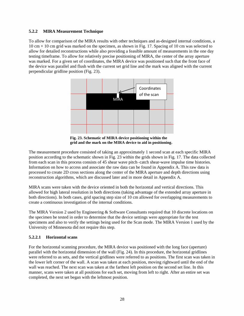
5.2.2 MIRA Measurement Technique
To allow for comparison of the MIRA results with other techniques and as-designed internal conditions, a
10 cm × 10 cm grid was marked on the specimen, as shown in Fig. 17. Spacing of 10 cm was selected to
allow for detailed reconstructions while also providing a feasible amount of measurements in the one day
testing timeframe. To allow for relatively precise positioning of MIRA, the center of the array aperture
was marked. For a given set of coordinates, the MIRA device was positioned such that the front face of
the device was parallel and flush with the current set grid line and the mark was aligned with the current
perpendicular gridline position (Fig. 23).
Fig. 23. Schematic of MIRA device positioning within the
grid and the mark on the MIRA device to aid in positioning.
The measurement procedure consisted of taking an approximately 1 second scan at each specific MIRA
position according to the schematic shown in Fig. 23 within the grids shown in Fig. 17. The data collected
from each scan in this process consists of 45 shear wave pitch–catch shear-wave impulse time histories.
Information on how to access and associate the raw data can be found in Appendix A. This raw data is
processed to create 2D cross sections along the center of the MIRA aperture and depth directions using
reconstruction algorithms, which are discussed later and in more detail in Appendix A.
MIRA scans were taken with the device oriented in both the horizontal and vertical directions. This
allowed for high lateral resolution in both directions (taking advantage of the extended array aperture in
both directions). In both cases, grid spacing step size of 10 cm allowed for overlapping measurements to
create a continuous investigation of the internal conditions.
The MIRA Version 2 used by Engineering & Software Consultants required that 10 discrete locations on
the specimen be tested in order to determine that the device settings were appropriate for the test
specimens and also to verify the settings being used for the Scan mode. The MIRA Version 1 used by the
University of Minnesota did not require this step.
5.2.2.1 Horizontal scans
For the horizontal scanning procedure, the MIRA device was positioned with the long face (aperture)
parallel with the horizontal dimension of the wall (Fig. 24). In this procedure, the horizontal gridlines
were referred to as sets, and the vertical gridlines were referred to as positions. The first scan was taken in
the lower left corner of the wall. A scan was taken at each position, moving rightward until the end of the
wall was reached. The next scan was taken at the farthest left position on the second set line. In this
manner, scans were taken at all positions for each set, moving from left to right. After an entire set was
completed, the next set began with the leftmost position.
MIRA
Coordinates
of the scan

29
Fig. 24. Horizontal scanning procedure.
A total of 14 sets and 17 positions were used in the horizontal scanning procedure (Fig. 25). While
Specimen 6 dimensions are used for illustration purposes, the same procedure was used for Specimen 2
although the dimensions of the slab were slightly different. When taking the first and last scans for each
set line, the device was placed so that all of the array sensors were in contact with the specimen. The
bottom and top scans were taken with additional room from the edge to minimize structural noise from
the specimen boundary. Therefore, the first position line considered was centered at the 20.32 cm
position, and the rightmost scan was centered at the 1.83 m position. The distance from the center of the
device to the outer edge of the array allowed for the 17 positions to cover the entire width of the
specimen. The sets (denoted by red arrows) correspond to the cross sections covered by the extended
reconstructions (SAFT-Panoramic), which is introduced later and detailed in Appendix A.
5.2.2.2 Vertical scans
For the vertical scanning procedure, the MIRA device was positioned with the array aperture parallel with
the vertical dimension of the wall (Fig. 26). In this procedure, the vertical gridlines were referred to as
sets, and the horizontal gridlines were referred to as positions (note that this is the opposite naming
convention as used in the horizontal scanning procedure). The first scan was taken in the lower right
corner of the wall with the front of the device facing toward the left side of the slab. A scan was taken at
each position, moving upwards until the top of the wall was reached. The next scan was taken at the
bottommost position on the second set line, 10 cm to the left of the first set line. In this manner, scans
were taken at all positions for each set, moving from bottom to top. After an entire set was completed, the
next set began with the bottom position.
A total of 20 sets and 11 positions were used in the horizontal scanning procedure (Fig. 27). Similar to the
horizontal scanning procedure, the first and last scans for each set line were centered 20 cm from the
edge. Therefore, the 11 positions covered the entire vertical span of the specimens. The sets (denoted by
red arrows) correspond to the cross sections covered by the extended reconstructions (SAFT-Panoramic).

30
Fig. 25. Sets and positions used in the horizontal scanning procedure.
Fig. 26. Vertical scanning procedure.
Specimen #7: Horizontal
Set 1
Set 2
Set 3
Set 4
Set 5
Set 6
Set 7
Set 8
Set 9
Set 10
Set 11
Set 12
Set 13
Set 14
4 in.
8 in.
12 in.
16 in.
20 in.
24 in.
28 in.
32 in.
36 in.
40 in.
44 in.
48 in.
52 in.
56 in.
8 in. 16 in. 24 in. 32 in. 40 in. 48 in. 56 in. 64 in. 72 in. 80 in.
Pos 1 Pos 5 Pos 9 Pos 13 Pos 17

31
Fig. 27. Sets and positions used in the vertical scanning procedure.
5.2.2.3 MIRA Version 1 reconstruction
The measurement procedure allowed for analysis using various reconstruction methods designed to focus
peaks in the reflected impulses to the locations of changes in acoustic impedance within the specimen.
Details on how to create the reconstructions from the individual shear wave impulse time histories can be
found in Appendix A.
The following analyses were conducted with reference to additional details in Appendix A.
Full waveform reconstructions (SAFT-FW) – see Section A.1 of Appendix A
Instantaneous amplitude reconstructions (SAFT-IA B-scans) – see Section A.3
3D reconstructions (SAFT-3D) – see Section A.4
Extended virtual array (SAFT-Panoramic) – see Section A.5
Automated detection of concrete thickness (direct reflection automation) – see Section A.7
5.3 ANTARES EQUIPMENT SETUP AND MEASUREMENT TECHNIQUES
5.3.1 ANTARES Overview
ANTARES is a comprehensive hardware, software, and support package designed to robotically perform
high resolution NDE on concrete structures, and to impartially evaluate NDE instruments for
effectiveness in analyzing structural properties and defects of interest to the FDOT.
ANTARES was born out of a postdoctoral research project by Dr. Daniel Algernon, who serves as a
special consultant to ongoing FDOT research efforts. The original automated NDE system was designed
to validate NDE instruments used in the State of Florida in a manner that all but eliminated human error
from the data collection process. The ANTARES system expands this system with new instruments,
enhanced flexibility, improved interfaces, simplified operation, and greater capability for field
deployment to collect real-world structural NDE data.
Specimen #7: Vertical
Pos 1
Pos 2
Pos 3
Pos 4
Pos 5
Pos 6
Pos 7
Pos 8
Pos 9
Pos 10
Pos 11
4 in.
8 in.
12 in.
16 in.
20 in.
24 in.
28 in.
32 in.
36 in.
40 in.
44 in.
48 in.
52 in.
56 in.
8 in. 16 in. 24 in. 32 in. 40 in. 48 in. 56 in. 64 in. 72 in. 80 in.Set 20 Set 15 Set 10 Set 5 Set 1
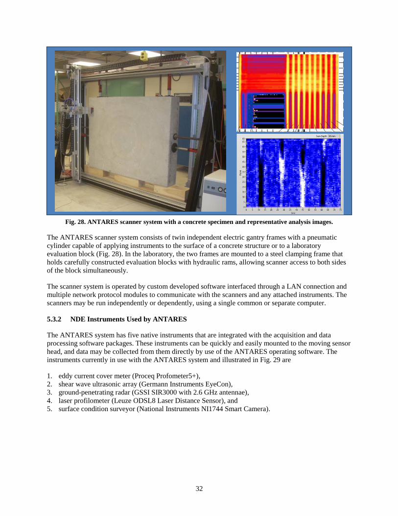
32
Fig. 28. ANTARES scanner system with a concrete specimen and representative analysis images.
The ANTARES scanner system consists of twin independent electric gantry frames with a pneumatic
cylinder capable of applying instruments to the surface of a concrete structure or to a laboratory
evaluation block (Fig. 28). In the laboratory, the two frames are mounted to a steel clamping frame that
holds carefully constructed evaluation blocks with hydraulic rams, allowing scanner access to both sides
of the block simultaneously.
The scanner system is operated by custom developed software interfaced through a LAN connection and
multiple network protocol modules to communicate with the scanners and any attached instruments. The
scanners may be run independently or dependently, using a single common or separate computer.
5.3.2 NDE Instruments Used by ANTARES
The ANTARES system has five native instruments that are integrated with the acquisition and data
processing software packages. These instruments can be quickly and easily mounted to the moving sensor
head, and data may be collected from them directly by use of the ANTARES operating software. The
instruments currently in use with the ANTARES system and illustrated in Fig. 29 are
1. eddy current cover meter (Proceq Profometer5+),
2. shear wave ultrasonic array (Germann Instruments EyeCon),
3. ground-penetrating radar (GSSI SIR3000 with 2.6 GHz antennae),
4. laser profilometer (Leuze ODSL8 Laser Distance Sensor), and
5. surface condition surveyor (National Instruments NI1744 Smart Camera).

33
Fig. 29. Various instruments installed on the ANTARES system.
A unique feature of the ANTARES system is the ability to use nonnative instruments operated in
“parallel.” In parallel operation mode, the ANTARES operating software moves the scanner systems in
accordance with the user-defined testing grid. The parallel instrument is mounted to the sensor head using
a standardized aluminum bracket and collects data independently of the scanner system. With the
ANTARES post processing software, almost any data collected by a parallel instrument can be opened,
processed, and meshed to the grid file outputted by the ANTARES operating software.
5.3.3 Applications for Structures and Materials
5.3.3.1 Laboratory
The ANTARES system retains the original purpose and functionality of the automated NDE program for
validation of field-deployable NDE instruments. By incorporating the parallel operation mode, this
application as an FDOT Structural NDE Validation Facility is easier than ever before. Instrument
manufacturers and NDE testing firms can have their instruments and techniques impartially judged by a
system that removes human error from the placement and location process and evaluates NDE
effectiveness on a wide variety of simulated defects, structural features, and known material properties.
Instruments can be validated using the most impartial system available operated by an equally impartial
government agency.
[1] [2]
[3]
[4] [5]

34
5.3.3.2 Field
The ANTARES program shows great potential for field use as a tool for both quality control and forensic
applications. Treated strictly as an automated data collection tool, this system offers a rapid and
repeatable method available for collecting large numbers of data points in extremely dense grids. Most
importantly, the automated method of data collection reduces the potential for operator error and produces
data that is dense, detailed, repeatable, and defensible.
The ANTARES system can be mounted in any orientation using concrete anchors and special brackets.
The system can be deployed on structural elements in use or immediately after production for quality
control applications. Additionally, the use of the Surface Condition Surveyor instrument allows intelligent
orientation of the scanner system, using specially designed aluminum placards affixed to the specimen to
be scanned. The placards are printed with an origin graphic and spatial calibration grid that is used with
vision processing algorithms to provide the post processing software with a spatial transformation matrix
used to overlay scans taken at different times and different orientations with extremely high repeatability.
5.3.4 Continued Research
As such a unique, versatile, and accessible system, the ANTARES system promises massive potential for
continued research into NDE. The ANTARES software is developed from scratch in National Instruments
LabVIEW, and the source code is available for future researchers for expansion and modification.
Evaluation block molds, interfacing protocols for new instruments, designs for mounting hardware, etc.
are all retained by Lynch & Ferraro Engineering, Inc. (LFE) for use by future research efforts into
automated NDE. Some potential research efforts include, but are not limited to,
Incorporation of new instruments with minimal development time
Probability of Detection (POD) studies with unprecedented speed and accuracy
Applications for precast/pre-stress industries (rapid quality control)
Incorporation of deep flaw detection for mass, nuclear applications
Further refinement of vision-based data acquisition for quantification of surface damage, irregularity
5.4 AIR-COUPLED AND SEMI-COUPLED ULTRASONIC EQUIPMENT SETUP AND
MEASUREMENT TECHNIQUES
5.4.1 Air-Coupled Impact Echo
Air-coupled impact echo tests were carried out using conventional testing equipment, as shown in Fig. 30.
An impact event was applied to the surface of the concrete slab at a point using a steel ball impactor with
a diameter of 12 mm. The resulting vibration response was monitored nearby using an air-coupled sensor
(dynamic microphone) [8]. The air-coupled sensor measures air pressure resulting from the dynamic
response, where each event is represented by a time signal with 5 ms duration. The data were collected
using a 16 bit digitizer at a sampling rate of 1 MS/s. The digitized data were stored and processed on a
computer (Fig. 30). Each time, the signal is mapped to the frequency domain (amplitude spectrum) using
a Fast Fourier Transform algorithm with a spectral line spacing of 200 Hz. Impact-echo data were
collected along a 10 cm and 5cm square grid across the front face of Specimens 2 and 6, respectively. It
took approximately 120 minutes to scan the entire face of each specimen.

35
Fig. 30. Illustration of equipment used for air-coupled impact-echo tests.
(Note: Tests carried out with slabs oriented vertically.)
5.4.2 Air-Coupled Ultrasonic Surface Wave
The ultrasonic surface wave tests were carried out using specially designed testing equipment, which is
shown in Fig. 31. The hardware was designed and fabricated from components by the investigators. An
electrostatic air-coupled transducer emits an ultrasonic pulse with a center frequency of 60 kHz. The
emitted wave pulse is directed at the concrete surface at the critical angle (approximately 8 degrees from
vertical), initiating a surface wave that propagates along the surface. The propagating surface wave causes
surface motion in the solid that “leaks” energy into the air, which is detected by a linear array of four
MEMs microphone sensors spaced at 1 cm. The sensing and receiving transducers are positioned 80 mm
above the surface. The received time signals were averaged 100 times, and then digitized using a 32-bit
digitizer at a sampling rate of 2 MS/s. The digitized data were stored and processed on a computer.
Ultrasonic surface wave data were collected along a 5.08 cm square grid across the front face of the
specimen. Because the size of the testing array is larger than the scan grid, there is approximately 3 cm
overlap in the projections of the test configuration footprint on the surface. It took 384 minutes to scan the
entire face of each specimen, including the time needed to set up and move the scanning frame between
tests. The digitized time signal data were analyzed to determine an arrival time and first peak amplitude of
each averaged signal, as shown in Fig. 31; note that each testing position produces four time signals, sent
by the sending transducer and received by each sensor in the array. For each received signal, arrival time
and signal amplitude of the surface wave pulse were measured. Arrival time was indicated by the first
leading edge arrival of the pulse. The pulse arrival time was automatically determined for each signal
using a statistics-based criterion, which calculates reasonable threshold value based on the character of
the noise region before P-wave arrival within each time signal [9]. This computation was carried out
using a Matlab routine designed by the investigators. The amplitude was defined as the amplitude of the
first positive peak in the pulse after the defined pulse arrival time; this value was also determined
automatically for each signal. The automatic signal arrival time and amplitude estimations were carried
out using a Matlab software routine.
DAQ equipment
Air-coupled sensor(dynamic microphone)
Hardened steel ball impactor
Data acquisition system

36
Fig. 31. Illustration of air-coupled ultrasonic surface wave method: bottom-side view of sending and receiving
transducer set (left); view of data acquisition equipment and sensor net mounted in scanning frame for tests
(center); illustration of signal data collection analysis (right).
It should be noted that surface waves propagate along the surface of the concrete and do not extend
deeply into the depth of concrete. As a rule of thumb, surface waves interrogate and interact with the solid
to a depth of approximately one wavelength. In this case, the wave pulse has a center frequency of
60 kHz, so the expected interrogation depth is approximately 6 to7 cm. Surface waves cannot interrogate
deeply into the structure and only provide near-surface results.
5.4.3 Semi-Coupled Ultrasonic Tomography
The through-thickness ultrasonic tomography tests were carried out using specially designed testing
equipment, shown in Fig. 32. An electrostatic air-coupled transducer emits an ultrasonic pulse having a
center frequency of 50 kHz. The emitted wave pulse is directed at the concrete surface normal to the
surface, initiating a compressional wave (P-wave) that propagates into the thickness of the specimen. A
second nearby electrostatic transducer sends and receives a separate ultrasonic pulse which reflects from
the top surface of the sample in order to accurately determine the transmitting sensor height above the
surface. An accurate estimate of sensor height is needed to compute the travel time of the through-
thickness pulse in the material. The propagating P-wave pulse is detected by an array of eight
accelerometers, which are directly attached on the back side (opposing) of the sample. The accelerometers
have nominal sensitivity of 10 mV/g with a height and width of 10.9 mm and 7.6 mm, respectively. The
accelerometers are positioned in two parallel rows of four sensors each, with 10.16 cm spacing between
sensors within one row and 20.32 cm spacing between rows. The eight accelerometers define a 45.72 cm
× 20.32 cm scan zone sub-block volume within the total volume of the test sample, as illustrated in Fig.
33. Within each scan zone sub-block, data are collected to reconstruct five different tomographic slice
images within the block. To construct these five slice images, one of the accelerometer line sets must be
moved once, and the sending transducer scan repeated. The sending transducers are positioned
approximately 7.5 cm above the surface. The received time signals from each accelerometer were
averaged 30 times, and then digitized using a 32-bit digitizer at a sampling rate of 2 MS/s. The digitized
data were stored and processed on a personal computer. The ultrasonic sending transducer was moved in
1.72 cm increments across the front face of the sample in three separate horizontal scans separated by
10.16 cm vertical spacing within each scan sub-block zone. It took 15 minutes to collect data for each
scan zone sub-block. It took 400 minutes to scan the entire sample, which is made up of 24 scan zone sub-
blocks, including the time needed to set up and move the scanning frame and re-mount the accelerometer
sets between tests. The digitized time signal data were analyzed to determine a P-wave arrival time for
each averaged time signal. The P-wave arrival time was automatically determined for each signal using a
Arrival Time of 1st peak
R1
…..
R2 R3
1st peak
R4
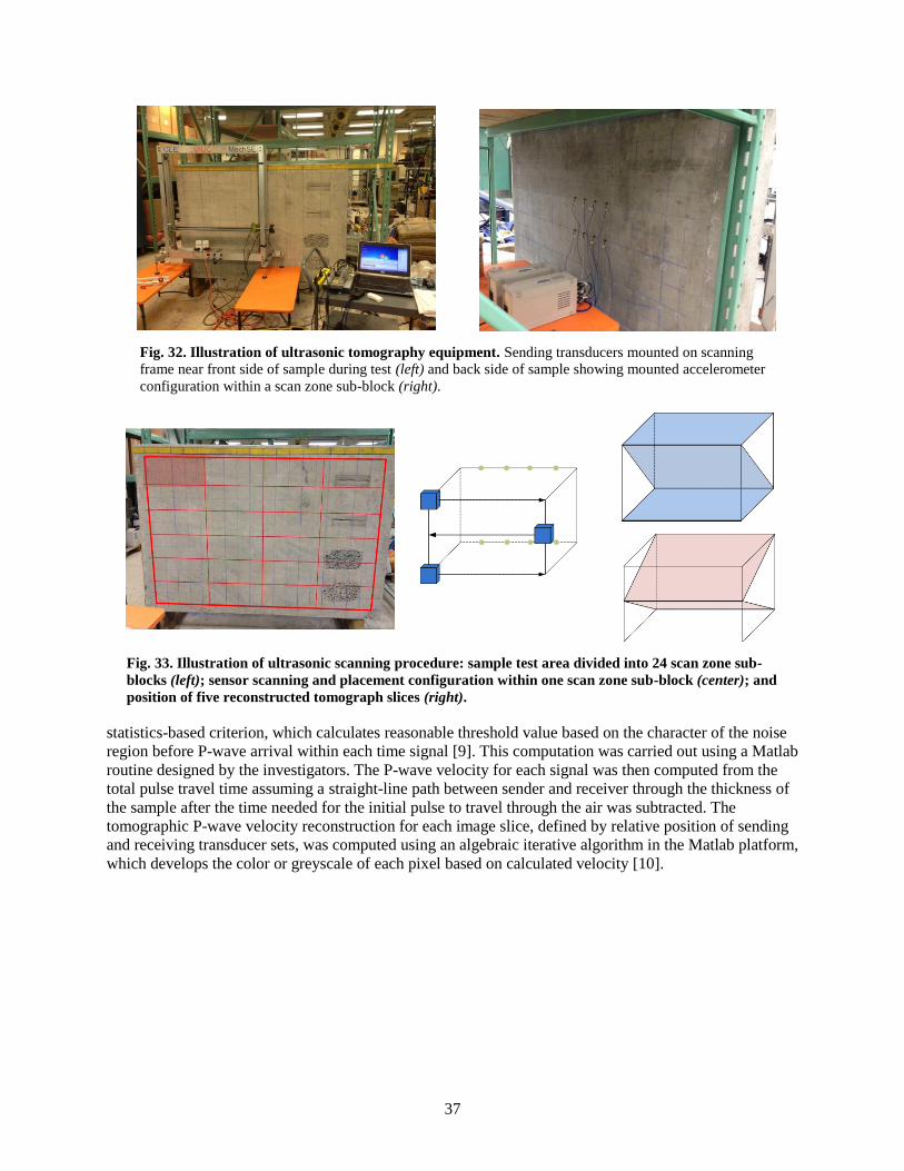
37
Fig. 32. Illustration of ultrasonic tomography equipment. Sending transducers mounted on scanning
frame near front side of sample during test (left) and back side of sample showing mounted accelerometer
configuration within a scan zone sub-block (right).
Fig. 33. Illustration of ultrasonic scanning procedure: sample test area divided into 24 scan zone sub-
blocks (left); sensor scanning and placement configuration within one scan zone sub-block (center); and
position of five reconstructed tomograph slices (right).
statistics-based criterion, which calculates reasonable threshold value based on the character of the noise
region before P-wave arrival within each time signal [9]. This computation was carried out using a Matlab
routine designed by the investigators. The P-wave velocity for each signal was then computed from the
total pulse travel time assuming a straight-line path between sender and receiver through the thickness of
the sample after the time needed for the initial pulse to travel through the air was subtracted. The
tomographic P-wave velocity reconstruction for each image slice, defined by relative position of sending
and receiving transducer sets, was computed using an algebraic iterative algorithm in the Matlab platform,
which develops the color or greyscale of each pixel based on calculated velocity [10].


39
6. SIGNAL INTERPRETATION/RESULT
6.1 MIRA VERSION 1 – UNIVERSITY OF MINNESOTA
MIRA was used to scan two concrete specimens following the grid pattern described in the methods
section. The procedures referenced in the analysis section and detailed in appendix A were used to
transform the raw MIRA data into reconstructions of the specimen internal components. Some example
characteristics of interest from initial analysis of these specimens are given in this section.
6.1.1 MIRA Version 1 Analysis of Specimen 6
Table 3 shows the features in the wall detected by interpreting the ultrasonic reconstruction and in some
cases (such as the consolidation and cracks) by visual survey of Specimen 6. The features were all
detected from the interpretation of the various reconstruction types from the analysis section.
Table 3. Feature in Specimen 6 as detected by MIRA
Feature Horizontal Location Vertical Location
Reinforcement #1 (R1) ~27 in. From 0 in. to 80 in. (entire span)
Reinforcement #2 (R2) ~40 in. From 0 in. to 80 in. (entire span)
Reinforcement #3 (R3) ~53 in. From 0 in. to 80 in. (entire span)
Poorly Consolidated Concrete (PC1) From 8 in. to 18 in. From 9 in. to 15 in.
Poorly Consolidated Concrete (PC2) From 8 in. to 18 in. From 20 in. to 26 in.
Crack #1 (CR1) From 8 in. to 18 in. ~34 in.
Crack #2 (CR2) From 8 in. to 18 in. ~46 in.
Each SAFT-Panoramic reconstruction created from MIRA data corresponds to one row on the grid shown
in Fig. 34. There were three inclusion reflections, consistent with characteristics of reinforcements with
various degrees of surrounding concrete conditions, and will be referred to as reinforcements 1 through 3
herein (R1,R2,R3). The poor consolidation and cracks that can be observed on the back side of Specimen
6 are referred to as PC1, PC2, CR1, and CR2, respectively (see Fig. 32). In each of the reconstructions,
the cross section is a slice through the thickness of the wall with the 0 in. at the top representing the front
face of the wall, where the MIRA device was placed during testing. When imaging the entire depth the
high relative reflectivity locations at approximately 10 in. are caused by the interface between the back
face of the concrete specimen and air. This reflection is referred to as the “back wall” herein. Examples of
reconstructions and signal interpretations used to detect some of the internal characteristics of the wall are
presented below.
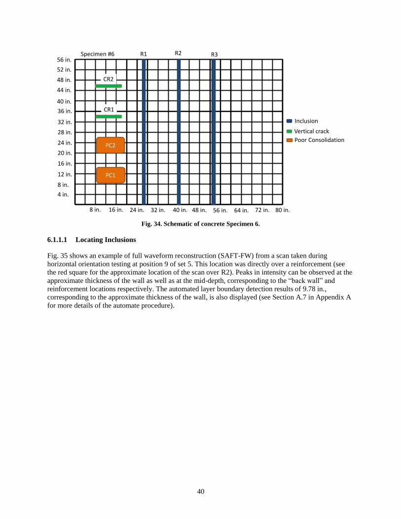
40
Fig. 34. Schematic of concrete Specimen 6.
6.1.1.1 Locating Inclusions
Fig. 35 shows an example of full waveform reconstruction (SAFT-FW) from a scan taken during
horizontal orientation testing at position 9 of set 5. This location was directly over a reinforcement (see
the red square for the approximate location of the scan over R2). Peaks in intensity can be observed at the
approximate thickness of the wall as well as at the mid-depth, corresponding to the “back wall” and
reinforcement locations respectively. The automated layer boundary detection results of 9.78 in.,
corresponding to the approximate thickness of the wall, is also displayed (see Section A.7 in Appendix A
for more details of the automate procedure).
Specimen #6
4 in.
8 in.
12 in.
16 in.
20 in.
24 in.
28 in.
32 in.
36 in.
40 in.
44 in.
48 in.
52 in.
56 in.
8 in. 16 in. 24 in. 32 in. 40 in. 48 in. 56 in. 64 in. 72 in. 80 in.
Inclusion
Vertical crack
Poor ConsolidationPC2
PC1
R1 R2 R3
CR1
CR2

41
Fig. 35. Example SAFT-FW scan along with automated layer boundary detection results.
A combination of the overlapping scan procedure and extended virtual array reconstruction procedure,
SAFT-Panoramic or SAFT-Epan (detailed in Sections A.5. and A.9., respectively) allows for a
continuous reconstruction of the entire span of the specimen. Fig. 36 shows an illustration of the SAFT-
Panoramic results created from horizontal scanning procedure set 5 measurements, which spans the
horizontal components of the specimen, including three reinforcements. The location of the SAFT-
Panoramic reconstruction is denoted by the translucent red box. It can be observed from Fig. 36(a) that, in
addition to the deeper continuous back wall reflection, there are three circular higher relative reflectivity
locations, corresponding to the reinforcement locations. A zoomed and higher threshold view of the
reinforcements can be observed in Fig. 36(c) and outlined in red in Fig. 36(a). These three inclusions
located at approximately mid-depth of the specimen are consistent with what should be expected from a
grouted reinforcement at horizontal locations of approximately 27 in., 40 in., and 53 in.
Inclusion Reflection
Backwall Reflection
Specimen #7
4 in.
8 in.
12 in.
16 in.
20 in.
24 in.
28 in.
32 in.
36 in.
40 in.
44 in.
48 in.
52 in.
56 in.
8 in. 16 in. 24 in. 32 in. 40 in. 48 in. 56 in. 64 in. 72 in. 80 in.
Inclusion
Vertical crack
Poor ConsolidationPC2
PC1
TD1 TD2 TD3
CR1
CR2

42
Fig. 36. Schematic of wall specimen 6 and MIRA reconstructions at the location specified in the schematic
showing reinforcements.
By extending the reconstruction in both the horizontal and vertical directions, further information about
the internal components of the concrete structure can be obtained. Fig. 37 shows the SAFT-3D
reconstruction of the specimen, where it can be observed that the three reinforcements extend the entire
span of the specimen.
Fig. 37. SAFT 3D reconstruction of reinforcements.
6.1.1.2 Characterizing inclusions
In addition to locating inclusions such as reinforcements, the characteristics of the inclusion can also be
evaluated. The leftmost reinforcement (R1) provides a good example of changing characteristics of an
internal component of the concrete structure. Fig. 38(a) shows the same SAFT-Panoramic reconstruction
Specimen #1
4 in.
8 in.
12 in.
16 in.
20 in.
24 in.
28 in.
32 in.
36 in.
40 in.
44 in.
48 in.
52 in.
56 in.
8 in. 16 in. 24 in. 32 in. 40 in. 48 in. 56 in. 64 in. 72 in. 80 in.
Inclusion
Vertical crack
Poor Consolidation
Inclusions
Zoomed in View
(a)
(b)(c)
R1R2
R3

43
along with three additional zoomed in vertical locations along R1 [Fig. 38 (c)]. The locations along R1
are denoted by translucent purple squares at vertical locations 20 in., 32 in., and 40 in., and labeled I1, I2,
and I3, respectively. It can be observed that the size and intensity of the reflectivity along R1 is increasing
as the vertical location increases. This is the type of trend you should expect from a fully bonded sound
surrounding concrete condition which is transitioning to an inclusion condition with damage in the
surrounding concrete. This is due to the increase in dimensions of the reflecting interface for the
ungrouted condition as well as the higher change in acoustic impedance and subsequent reflection
coefficient, caused by transitioning from concrete to air versus concrete to steel. When conducting this
type of analysis it is important to account for variability in amplitude due to the contact conditions. In this
study, normalizing to the direct shear wave arrival was conducted to address this issue.
Fig. 38. Schematic of concrete specimen 6 and MIRA reconstructions at the locations specified in the
schematic showing reinforcements.
The changing characteristics of the inclusion can also be inferred by evaluating the back wall condition
along R1. Fig. 39(a) shows the same SAFT-Panoramic reconstruction along with three additional zoomed
in vertical locations along R1 [Fig. 39(b)]. The locations along R1 are denoted by translucent purple
squares at vertical locations 20 in., 32 in., and 40 in., and labeled I1, I2, and I3, respectively. By zooming
in on the deeper portion of the scans, it can be observed that there is a gap in the back wall reflection at
the higher vertical locations. Of course, the back wall of the concrete specimen does not have a gap at
these locations, suggesting that there is an obstacle blocking shear wave propagation from a significant
portion of the transducer pair measurements. A properly grouted reinforcement should not block enough
energy to cause this discontinuity or “shadowing” of the back wall reflection.
Leftmost Inclusion
Set 5
Set 8
Set 10
20 in.
32 in.
40 in.
(I1)
Vertical Dimension
(I2)
(I3)
in.
Vertical Set
Specimen #1
4 in.
8 in.
12 in.
16 in.
20 in.
24 in.
28 in.
32 in.
36 in.
40 in.
44 in.
48 in.
52 in.
56 in.
8 in. 16 in. 24 in. 32 in. 40 in. 48 in. 56 in. 64 in. 72 in. 80 in.
Inclusion
Vertical crack
Poor Consolidation
I3
I2
I1
(a)
(b)
(c)

44
Fig. 39. Schematic of concrete Specimen 6 reconstructions, including some locations with gaps at the
back wall indicating shadowing.
A combination of the overlapping scans in the vertical direction can also be used to create continuous
reconstructions of the entire vertical span of the specimen. Fig. 40 shows an illustration of the SAFT-
Panoramic results created from the vertical scanning procedure above R1. The translucent red box
denotes the location of the SAFT-Panoramic reconstruction. It can be observed from Fig. 40(a) that, in
addition to the back wall, reflection reduces and disappears starting at about the mid-height portion of the
specimen. Fig. 41(c) shows a zoomed in portion of the same vertical SAFT-panoramic location at the
depth of R1. It can be observed that there is an increase in relative reflectivity consistent with the results
shown in Fig. 41.
Leftmost Inclusion
Set 5
Set 8
Set 10
20 in.
32 in.
40 in.
(I1)
Vertical Dimension
(I2)
(I3)
in.
Vertical Set
Specimen #1
4 in.
8 in.
12 in.
16 in.
20 in.
24 in.
28 in.
32 in.
36 in.
40 in.
44 in.
48 in.
52 in.
56 in.
8 in. 16 in. 24 in. 32 in. 40 in. 48 in. 56 in. 64 in. 72 in. 80 in.
Inclusion
Vertical crack
Poor Consolidation
I3
I2
I1
Gap
(a)
(b)
(c)

45
Fig. 40. SAFT panoramic reconstruction in the vertical direction showing shadowing
at the higher vertical locations along R1.
Fig. 41. SAFT Panoramic reconstruction with a zoomed in portion showing the increase in relative
reflectivity towards the higher vertical location.
Full ShadowingDecreasing Backwall
Specimen #1
4 in.
8 in.
12 in.
16 in.
20 in.
24 in.
28 in.
32 in.
36 in.
40 in.
44 in.
48 in.
52 in.
56 in.
8 in. 16 in. 24 in. 32 in. 40 in. 48 in. 56 in. 64 in. 72 in. 80 in.
Inclusion
Vertical crack
Poor Consolidation
Specimen #1
4 in.
8 in.
12 in.
16 in.
20 in.
24 in.
28 in.
32 in.
36 in.
40 in.
44 in.
48 in.
52 in.
56 in.
8 in. 16 in. 24 in. 32 in. 40 in. 48 in. 56 in. 64 in. 72 in. 80 in.
Inclusion
Vertical crack
Poor Consolidation
Moderate relative reflectivity
Increased reflectivity
Inclusion Depth ~5 in.
(a)
(b)
(c)

46
A “bird’s eye” view of the SAFT 3D reconstruction is also useful in identifying the change in
characteristics of inclusion R1 at increase vertical locations as well as in comparison to the other
inclusions. In Fig. 42 it can be observed that the relative reflectivity at the top vertical half of R1 is larger
than all other inclusion locations. In Fig. 43 a different angle view of the SAFT 3D reconstruction shows
a portion of the back wall that is shadowed below the inclusion. This corresponds to the blocked shear
wave locations identified in the horizontal SAFT-Panoramic in Fig. 39 and the vertical SAFT-Panoramic
in Fig. 41.
Fig. 42. SAFT 3D reconstruction of Specimen 6 showing increased reflectivity of the top vertical half of R1.
Fig. 43. SAFT 3D reconstruction showing shadowing below the top vertical half of R1.
High reflectivity portion of R1
Shadowing
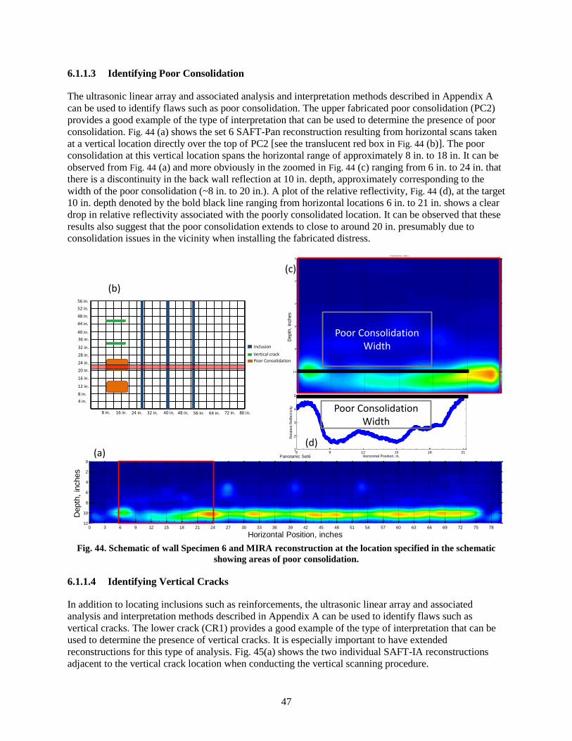
47
6.1.1.3 Identifying Poor Consolidation
The ultrasonic linear array and associated analysis and interpretation methods described in Appendix A
can be used to identify flaws such as poor consolidation. The upper fabricated poor consolidation (PC2)
provides a good example of the type of interpretation that can be used to determine the presence of poor
consolidation. Fig. 44 (a) shows the set 6 SAFT-Pan reconstruction resulting from horizontal scans taken
at a vertical location directly over the top of PC2 [see the translucent red box in Fig. 44 (b)]. The poor
consolidation at this vertical location spans the horizontal range of approximately 8 in. to 18 in. It can be
observed from Fig. 44 (a) and more obviously in the zoomed in Fig. 44 (c) ranging from 6 in. to 24 in. that
there is a discontinuity in the back wall reflection at 10 in. depth, approximately corresponding to the
width of the poor consolidation (~8 in. to 20 in.). A plot of the relative reflectivity, Fig. 44 (d), at the target
10 in. depth denoted by the bold black line ranging from horizontal locations 6 in. to 21 in. shows a clear
drop in relative reflectivity associated with the poorly consolidated location. It can be observed that these
results also suggest that the poor consolidation extends to close to around 20 in. presumably due to
consolidation issues in the vicinity when installing the fabricated distress.
Fig. 44. Schematic of wall Specimen 6 and MIRA reconstruction at the location specified in the schematic
showing areas of poor consolidation.
6.1.1.4 Identifying Vertical Cracks
In addition to locating inclusions such as reinforcements, the ultrasonic linear array and associated
analysis and interpretation methods described in Appendix A can be used to identify flaws such as
vertical cracks. The lower crack (CR1) provides a good example of the type of interpretation that can be
used to determine the presence of vertical cracks. It is especially important to have extended
reconstructions for this type of analysis. Fig. 45(a) shows the two individual SAFT-IA reconstructions
adjacent to the vertical crack location when conducting the vertical scanning procedure.
Panoramic Set6
Horizontal Position, inches
Depth
, in
ches
0 3 6 9 12 15 18 21 24 27 30 33 36 39 42 45 48 51 54 57 60 63 66 69 72 75 78
0
2
4
6
8
10
12
Panoramic Set6
Horizontal Position, inches
Depth
, in
ches
6 3 6 9 12 15 18
0
2
4
6
8
10
12
4 in.
8 in.
12 in.
16 in.
20 in.
24 in.
28 in.
32 in.
36 in.
40 in.
44 in.
48 in.
52 in.
56 in.
8 in. 16 in. 24 in. 32 in. 40 in. 48 in. 56 in. 64 in. 72 in. 80 in.
Inclusion
Vertical crack
Poor Consolidation
Poor Consolidation Width
(c)
(b)
(a) 6 9 12 15 18 211
2
3
4
5
Horizontal Position, in.
Re
lative
Re
fle
ctivity
(d)
Poor Consolidation Width

48
There is no clear indication of any discontinuity when looking at each individual scan. Contributing to the
difficulty in interpretation, the crack happened to be located at the outside portion of each scan making
the difference between shadowing and limited aperture difficult to resolve from one another.
Fig. 45. Schematic of concrete Specimen 6 and individual SAFT-IA
reconstructions at the CR1 location during vertical scanning.
shows the type of reconstructions and interpretation that can be used to significantly improve the clarity
and reliability of the analysis. Fig. 46(c) shows the SAFT Panoramic reconstruction corresponding to the
location shown by the translucent red box in Fig. 46(d) and Fig. 46(e). It can be observed that there is a
slight discontinuity in the back wall reflection at the crack location which becomes clearer when looking
at the zoomed in portion (outlined in the black box and shown in Fig. 46(b). Fig. 46(e) shows the
normalized relative reflectivity values along the black line portion of the box in Fig. 46(c) and Fig. 46(b).
In this case the dip in relative reflectivity is obvious at the location of the vertical crack.
Specimen #1
4 in.
8 in.
12 in.
16 in.
20 in.
24 in.
28 in.
32 in.
36 in.
40 in.
44 in.
48 in.
52 in.
56 in.
8 in. 16 in. 24 in. 32 in. 40 in. 48 in. 56 in. 64 in. 72 in. 80 in.
Inclusion
Vertical crack
Poor Consolidation
(a)
(b)
(c)

49
This highlights the importance of using the quantitative reconstruction matrix values rather than the
visual representations, which can be misleading or mask the characteristics of interest. Fig. 47 shows the
same type of analysis for CR2. The shadowing effect of this crack was more pronounced in the SAFT-
Panoramic reconstruction, although the relative reflectivity plot still assists in localizing the location of
the vertical crack.
Fig. 46. Use of SAFT-Panoramic and relative reflectivity measures to
identify a vertical crack.
0 20 40 60 80 100 120 140 160 1803.8
4
4.2
4.4
4.6
4.8
5
5.2
5.4
5.6
5.8
20 40 60 80 100 120 140 160
1
2
3
4
5
6
7
8
9
10
11
Rel
ativ
e R
efle
ctiv
ity
(a)
(b)
(c)
(d)
Specimen #1
4 in.
8 in.
12 in.
16 in.
20 in.
24 in.
28 in.
32 in.
36 in.
40 in.
44 in.
48 in.
52 in.
56 in.
8 in. 16 in. 24 in. 32 in. 40 in. 48 in. 56 in. 64 in. 72 in. 80 in.
Inclusion
Vertical crack
Poor Consolidation
(e)
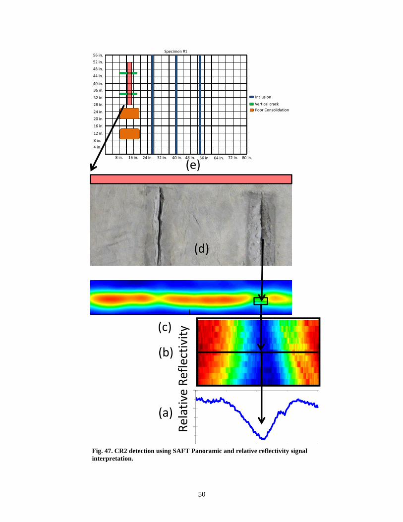
50
Fig. 47. CR2 detection using SAFT Panoramic and relative reflectivity signal
interpretation.
0 50 100 150 200 2502.5
3
3.5
4
4.5
5
5.5
10 20 30 40 50 60 70 80 90 100
1
2
3
4
5
6
7
8
9
10
11
Rel
ativ
e R
efle
ctiv
ity
(a)
(b)
(c)
(d)
Specimen #1
4 in.
8 in.
12 in.
16 in.
20 in.
24 in.
28 in.
32 in.
36 in.
40 in.
44 in.
48 in.
52 in.
56 in.
8 in. 16 in. 24 in. 32 in. 40 in. 48 in. 56 in. 64 in. 72 in. 80 in.
Inclusion
Vertical crack
Poor Consolidation
(e)
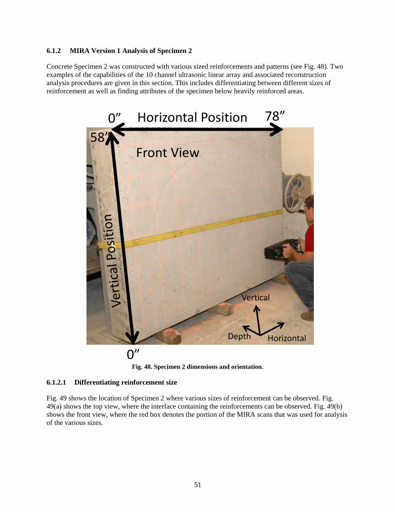
51
6.1.2 MIRA Version 1 Analysis of Specimen 2
Concrete Specimen 2 was constructed with various sized reinforcements and patterns (see Fig. 48). Two
examples of the capabilities of the 10 channel ultrasonic linear array and associated reconstruction
analysis procedures are given in this section. This includes differentiating between different sizes of
reinforcement as well as finding attributes of the specimen below heavily reinforced areas.
Fig. 48. Specimen 2 dimensions and orientation.
6.1.2.1 Differentiating reinforcement size
Fig. 49 shows the location of Specimen 2 where various sizes of reinforcement can be observed. Fig.
49(a) shows the top view, where the interface containing the reinforcements can be observed. Fig. 49(b)
shows the front view, where the red box denotes the portion of the MIRA scans that was used for analysis
of the various sizes.
Front View
Vertical
HorizontalDepth
58”
0”
78”0” Horizontal Position
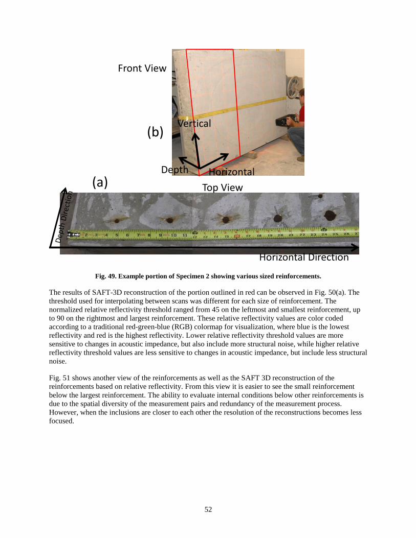
52
Fig. 49. Example portion of Specimen 2 showing various sized reinforcements.
The results of SAFT-3D reconstruction of the portion outlined in red can be observed in Fig. 50(a). The
threshold used for interpolating between scans was different for each size of reinforcement. The
normalized relative reflectivity threshold ranged from 45 on the leftmost and smallest reinforcement, up
to 90 on the rightmost and largest reinforcement. These relative reflectivity values are color coded
according to a traditional red-green-blue (RGB) colormap for visualization, where blue is the lowest
reflectivity and red is the highest reflectivity. Lower relative reflectivity threshold values are more
sensitive to changes in acoustic impedance, but also include more structural noise, while higher relative
reflectivity threshold values are less sensitive to changes in acoustic impedance, but include less structural
noise.
Fig. 51 shows another view of the reinforcements as well as the SAFT 3D reconstruction of the
reinforcements based on relative reflectivity. From this view it is easier to see the small reinforcement
below the largest reinforcement. The ability to evaluate internal conditions below other reinforcements is
due to the spatial diversity of the measurement pairs and redundancy of the measurement process.
However, when the inclusions are closer to each other the resolution of the reconstructions becomes less
focused.
Front View
Top View
Vertical
HorizontalDepth
Horizontal Direction
(b)
(a)

53
Fig. 50. A 3D reconstruction showing the various sized reinforcements.
Front View
Vertical
HorizontalDepth
Horizontal
Dep
th
(b)
(a)
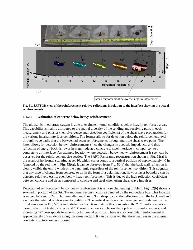
54
Fig. 51. SAFT 3D view of the reinforcement relative reflections in relation to the interface showing the actual
reinforcements.
6.1.2.2 Evaluation of concrete below heavy reinforcement
The ultrasonic linear array system is able to evaluate internal conditions below heavily reinforced areas.
This capability is mainly attributed to the spatial diversity of the sending and receiving pairs in each
measurement and physics (i.e., divergence and reflection coefficients) of the shear wave propagation for
the various internal interface conditions. The former allows for detection below the reinforcement level
through wave paths that are between adjacent reinforcements through multiple shear wave paths. The
latter allows for detection below reinforcements since the changes in acoustic impedance, and thus
reflection of energy back, is lower in magnitude at a concrete to steel interface in comparison to a
concrete to air interface. An example location where detection below heavy reinforcement is seen can be
observed for the reinforcement size section. The SAFT-Panoramic reconstruction shown in Fig. 52(a) is
the result of horizontal scanning at set 10, which corresponds to a vertical position of approximately 40 in
(denoted by the red line in Fig. 52(c)). It can be observed from Fig. 52(a) that the back wall reflection is
clearly visible the entire width of the panoramic regardless of the reinforcement condition. This suggests
that any type of change from concrete to air in the form of a delamination, flaw, or layer boundary can be
detected relatively easily, even below heavy reinforcement. This is due to the high reflection coefficient
between concrete and air as compared to concrete and steel when using shear wave impulses.
Detection of reinforcement below heavy reinforcement is a more challenging problem. Fig. 52(b) shows a
zoomed in portion of the SAFT-Panoramic reconstruction as denoted by the red outline box. This location
is ranged by 2 in. to 24 in. horizontally, and 0 in to 9 in. deep to crop the reflection from the back wall and
evaluate the internal reinforcement conditions. The vertical reinforcement arrangement is shown from a
top down view in Fig. 52(d) and labeled with a T# and B#. In this convention the “T” reinforcements are
close to the front testing surface and “B” reinforcements are below the top layer of reinforcements, and
increasing “#” corresponds to increasing horizontal position. There is also horizontal reinforcement at
approximately 8.5 in. depth along this cross section. It can be observed that these features in the internal
concrete structure are less focused.
Dep
th D
irec
tio
n
Dep
th, i
n.50
90
Small reinforcement below the larger reinforcement
(b)
(a)
T1T2 T3 T4 T5
B6
T1T2 T3 T4
T5
B6

55
However, there are slight increases in reflectivity in the general locations. For instance, while the
horizontal reinforcement extends throughout the width, there are slight circular oblong features at the
vertical reinforcements in the vicinity (B2, B3 and B4). B1, B5, and B6 are lower in magnitude, but give a
slight increase in reflectivity at the general location.
Fig. 52. Detection below heavy reinforcement.
6.2 MIRA VERSION 2 – ENGINEERING & SOFTWARE CONSULTANTS, INC.
The MIRA Version 2 system includes a laptop computer with software for 3D image visualization of the
B-scans acquired in the Scan mode. The software is known as IDealviewer.
IDealviewer takes the B-scans and “stitches” them together by using a signal processing technique known
as Synthetic Aperture Focusing Technique (SAFT) to reconstruct the internal structure of the concrete
specimen. This section describes the results obtained using a technique called Maximum Intensity
Projection (MIP).
MIP is a volume rendering technique that uses the ray casting technique to project the volume elements
with maximum intensity onto a viewing plane. MIP is ideal for putting out the high amplitude reflections
in the dataset, which in the present case is the most appropriate technique.
Panoramic Set10
Horizontal Position, inches
Depth
, in
ches
2 6 10 14 18 22
0
2
4
6
8
B1 B2B3
B4 B5B6T1 T2 T3 T4
B1 B2 B3B4
B5
B6
T1T2 T3 T4
Dep
th D
irec
tio
nD
epth
, in
.
Front View
Vertical
HorizontalDepth
58”
0”
78”0” Horizontal Position
(a)
(b)
(c) (d)
Horizontal reinforcement

56
6.2.1 Concrete Specimen 6 Horizontal Scan
Fig. 53(b) shows the MIP rendering of B-scans obtained from moving the MIRA horizontally along
concrete Specimen 6. For relevance, only 25.4 cm of the dataset is projected. It clearly shows the
response from three large rebar elements running vertically through the middle of the specimen. MIP also
does a good job of showing responses from honeycombing and cracking.
Fig. 53. (a) Front view of concrete Specimen 6; (b) 3D rendering showing the three large rebar elements
running vertically through the middle of the concrete specimen and the honeycomb on the left side of the
concrete specimen (as seen from the front view).
6.2.2 Concrete Specimen 6 Vertical Scan
Fig. 54(c) shows the MIP rendering of B-scans obtained from moving the MIRA vertically along concrete
Specimen 6. For relevance, only 25.4 cm of the dataset is projected. It clearly shows the response from
the flaw around the length of rebar 1. Response from honeycomb and cracks can also be seen; however,
the response from cracks is not very strong.

57
Fig. 54. (a) Front view of concrete Specimen 6; (b) top view of concrete Specimen 6; (c) 3D rendering shows
the honeycomb, cracks, and the large flaw around rebar 1.
Fig. 55(a) and Fig. 55(b) are stitched B-scans. These scans show the cross-sectional details of the flaws
obtained at the respective locations. Fig. 55(a) shows the response from honeycomb at the two locations;
however, the response from cracking is not very strong. Fig. 55(b) shows the response from the flaw
around the length of rebar 1.
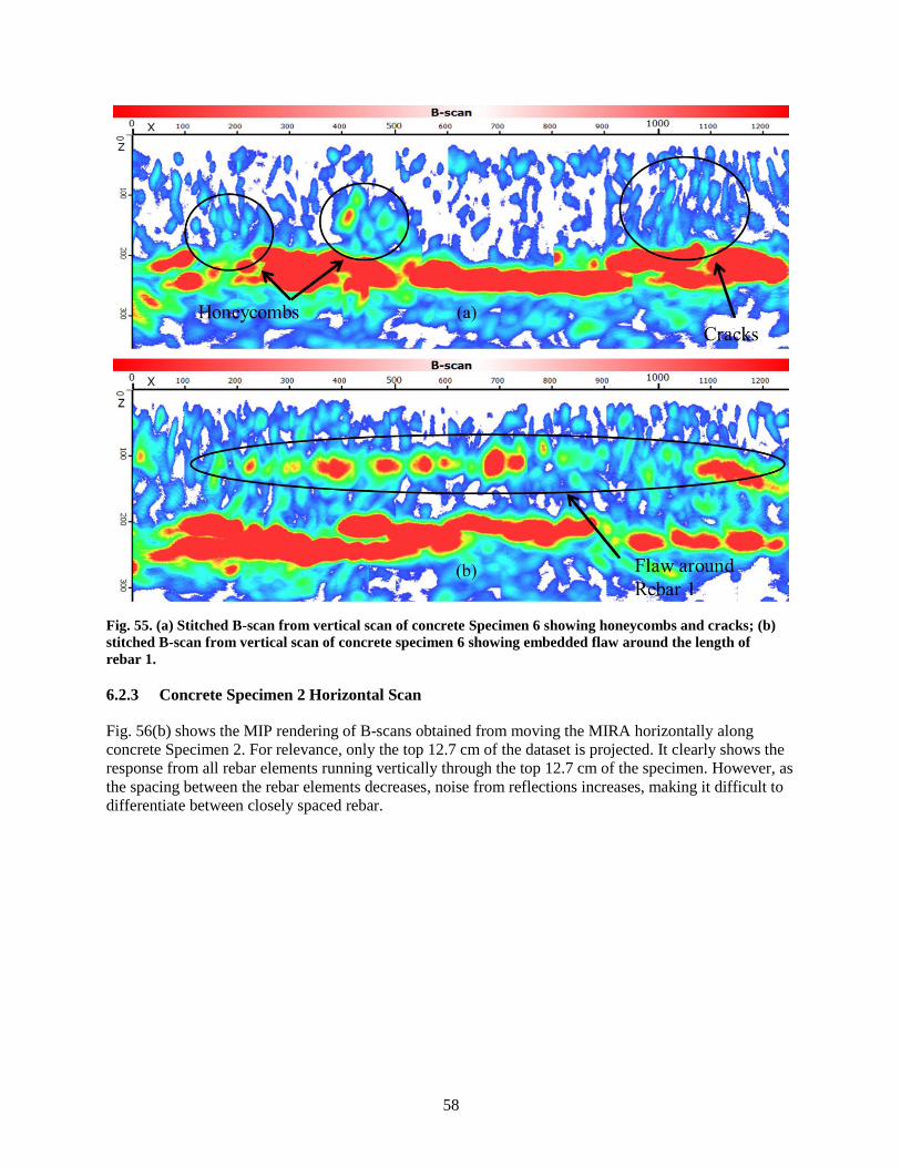
58
Fig. 55. (a) Stitched B-scan from vertical scan of concrete Specimen 6 showing honeycombs and cracks; (b)
stitched B-scan from vertical scan of concrete specimen 6 showing embedded flaw around the length of
rebar 1.
6.2.3 Concrete Specimen 2 Horizontal Scan
Fig. 56(b) shows the MIP rendering of B-scans obtained from moving the MIRA horizontally along
concrete Specimen 2. For relevance, only the top 12.7 cm of the dataset is projected. It clearly shows the
response from all rebar elements running vertically through the top 12.7 cm of the specimen. However, as
the spacing between the rebar elements decreases, noise from reflections increases, making it difficult to
differentiate between closely spaced rebar.
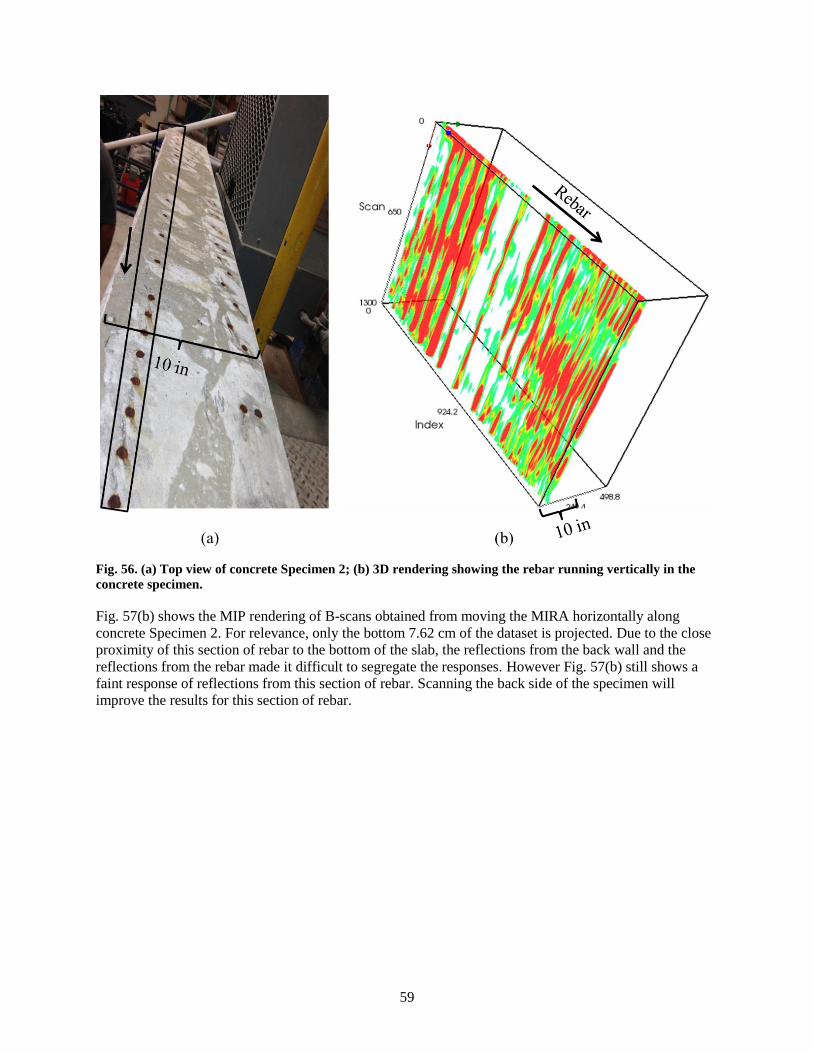
59
Fig. 56. (a) Top view of concrete Specimen 2; (b) 3D rendering showing the rebar running vertically in the
concrete specimen.
Fig. 57(b) shows the MIP rendering of B-scans obtained from moving the MIRA horizontally along
concrete Specimen 2. For relevance, only the bottom 7.62 cm of the dataset is projected. Due to the close
proximity of this section of rebar to the bottom of the slab, the reflections from the back wall and the
reflections from the rebar made it difficult to segregate the responses. However Fig. 57(b) still shows a
faint response of reflections from this section of rebar. Scanning the back side of the specimen will
improve the results for this section of rebar.
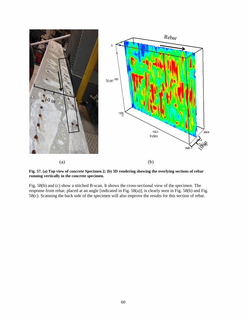
60
Fig. 57. (a) Top view of concrete Specimen 2; (b) 3D rendering showing the overlying sections of rebar
running vertically in the concrete specimen.
Fig. 58(b) and (c) show a stitched B-scan. It shows the cross-sectional view of the specimen. The
response from rebar, placed at an angle [indicated in Fig. 58(a)], is clearly seen in Fig. 58(b) and Fig.
58(c). Scanning the back side of the specimen will also improve the results for this section of rebar.

61
Fig. 58. (a) Top view of concrete Specimen 2; (b) 3D rendering showing the overlying sections of rebar
running vertically in the concrete specimen (c).
6.2.4 Concrete Specimen 2 Vertical Scan
Fig. 59(b) shows the MIP rendering of B-scans obtained from moving the MIRA vertically along concrete
Specimen 2. For relevance, only the top 12.7 cm of the dataset is projected. It clearly shows the response
from all rebar running horizontally through the top 12.7 cm of the specimen. However, as the spacing
between the rebar decreases, noise from reflections increases.

62
Fig. 59. (a) Side view of concrete Specimen 2; (b) 3D rendering shows the rebar running horizontally in the
concrete specimen close to the top of the slab.
Fig. 60(b) shows the MIP rendering of B-scans obtained from moving the MIRA vertically along concrete
Specimen 2. For relevance, only the bottom 7.62 cm of the dataset is projected. Due to the close
proximity of this section of rebar to the bottom of the slab, the reflections from the back wall and the
reflections from the rebar have become difficult to segregate. However, Fig. 60(b) still shows a faint
response of reflections from this section of rebar. Scanning the back side of the specimen will improve the
results for this section of rebar.
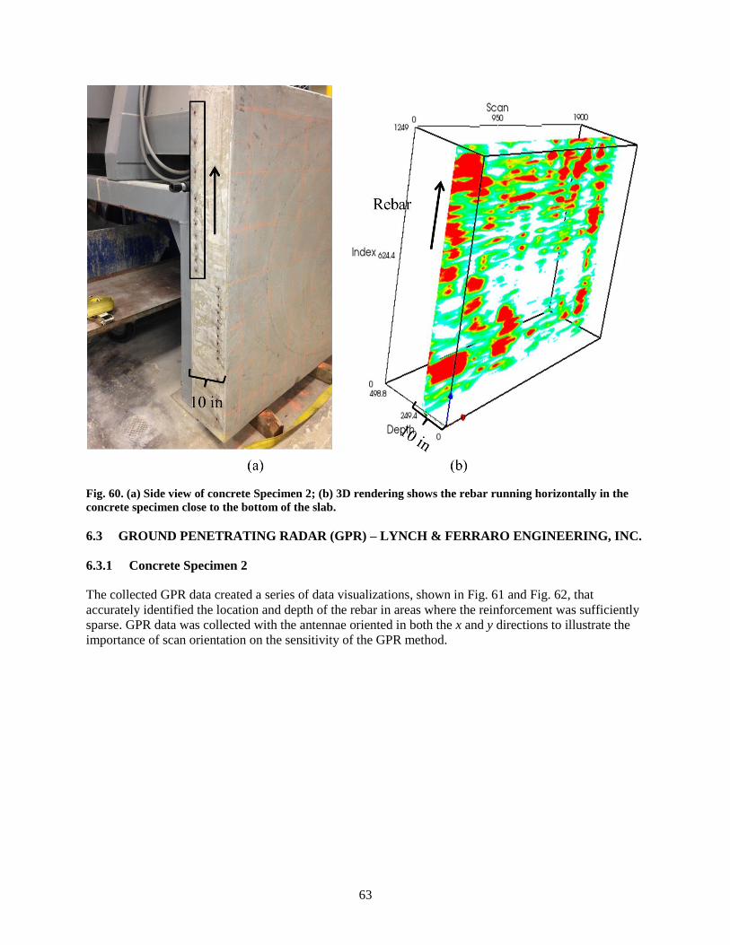
63
Fig. 60. (a) Side view of concrete Specimen 2; (b) 3D rendering shows the rebar running horizontally in the
concrete specimen close to the bottom of the slab.
6.3 GROUND PENETRATING RADAR (GPR) – LYNCH & FERRARO ENGINEERING, INC.
6.3.1 Concrete Specimen 2
The collected GPR data created a series of data visualizations, shown in Fig. 61 and Fig. 62, that
accurately identified the location and depth of the rebar in areas where the reinforcement was sufficiently
sparse. GPR data was collected with the antennae oriented in both the x and y directions to illustrate the
importance of scan orientation on the sensitivity of the GPR method.
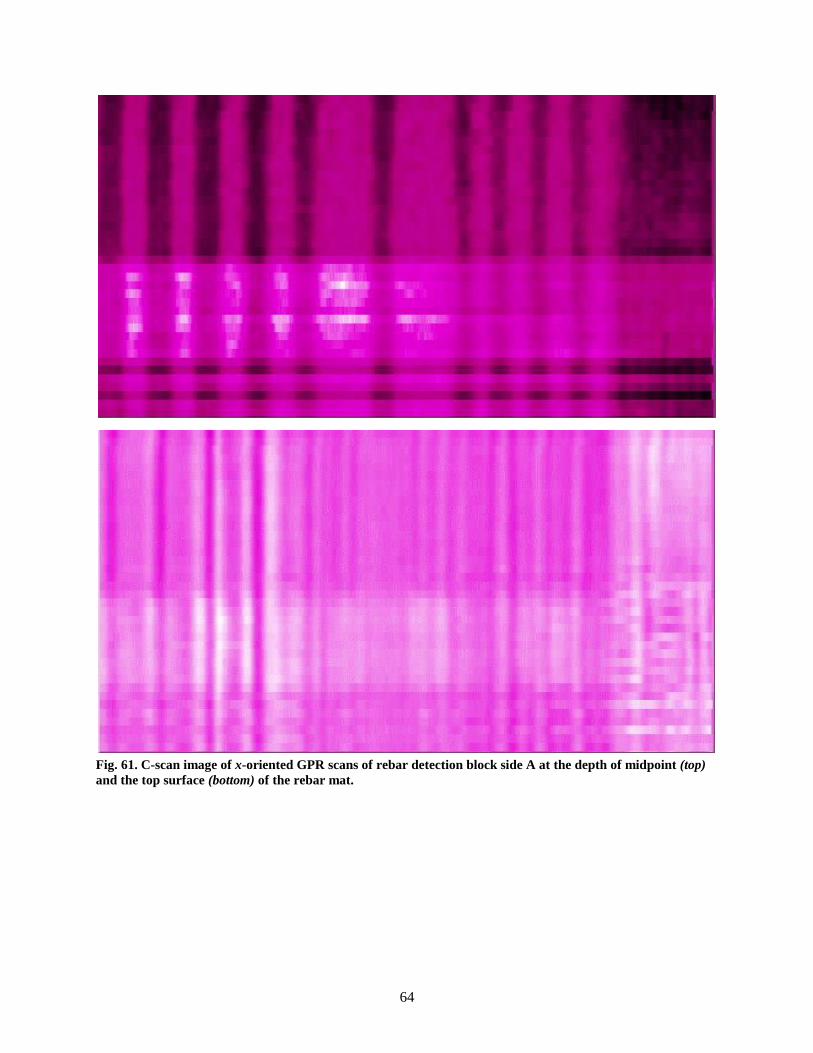
64
Fig. 61. C-scan image of x-oriented GPR scans of rebar detection block side A at the depth of midpoint (top)
and the top surface (bottom) of the rebar mat.

65
Fig. 62. C-scan image of y-oriented GPR scans of rebar detection block side A at the depth of midpoint (top)
and the top surface (bottom) of the top rebar mat.

66
6.3.2 Concrete Specimen 6
As expected, GPR scans of the void and flaw detection block revealed that radar is a generally ineffective
method for detecting all but the most severe internal air voids and defects. GPR quickly and accurately
located the three reinforcing bars in the void and flaw detection block, as shown in Fig. 63, and showed
clearly that one of the bars was badly out of place. GPR also identified the two most severe intentional
honeycomb defects embedded in the specimen as well as the artifacts from moving one of the three rebar
elements, though these indications are quite subtle as shown in Fig. 64.
Fig. 63. C-scan image of GPR scan of void and flaw detection block identifying the
three rebar elements and two locations of wave scattering due to internal
honeycombing. The leftmost rebar was pulled out-of-plane; an effect that is very apparent in
this image.
Fig. 64. GPR line scan showing a weak reflection of the leftmost rebar due to
delamination.

67
6.4 SHEAR WAVE ULTRASOUND DATA – LYNCH & FERRARO ENGINEERING, INC.
6.4.1 Concrete Specimen 2
While shear wave ultrasound is not traditionally used to locate reinforcing steel, the ANTARES system
produces sufficiently dense data to create detailed data visualization to make up for the poor sensitivity of
ultrasound to steel as shown in Fig. 65.
Fig. 65. C-scan image of ultrasound scan of rebar detection block side A with Hilbert transform visualization.
Shear wave ultrasound data is particularly dense and complex, and quite difficult to visualize using 2D
images. The ANTARES processing software was designed to visualize all data sets produced by the
ANTARES system but was developed primarily around shear wave ultrasound data. The software allows
the user to easily move through the depth of the C-scan image to better visualize the ways in which the
reflections of the ultrasound wave change and to more easily identify flaws and internal features. The
software allows precise location of defects in three dimensions using plot cursors as shown in Fig. 66 and
other features far beyond the data plots provided in this report. The images in this report are merely
intended as a visual representation of the scan results.

68
Fig. 66. Tomographic image of the xz plane of rebar block showing the two rebar layers as well as the section
of varying depth reinforcing steel. Here the cursor is used to identify the location of a particular bar in three
dimensions.
6.4.2 Concrete Specimen 6
In processing the ultrasound *.ANTDAT file, it was observed that that ultrasound reliably detected all of
the most severe defects. These defects were visible on the filter settings display shown in Fig. 67, which
only displays the depth of maximum reflection and is therefore usually unreliable at displaying all objects
of interest within a specimen.
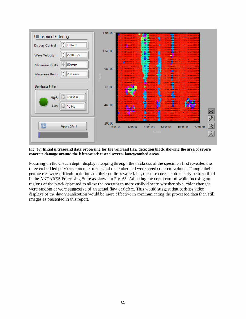
69
Fig. 67. Initial ultrasound data processing for the void and flaw detection block showing the area of severe
concrete damage around the leftmost rebar and several honeycombed areas.
Focusing on the C-scan depth display, stepping through the thickness of the specimen first revealed the
three embedded pervious concrete prisms and the embedded wet-sieved concrete volume. Though their
geometries were difficult to define and their outlines were faint, these features could clearly be identified
in the ANTARES Processing Suite as shown in Fig. 68. Adjusting the depth control while focusing on
regions of the block appeared to allow the operator to more easily discern whether pixel color changes
were random or were suggestive of an actual flaw or defect. This would suggest that perhaps video
displays of the data visualization would be more effective in communicating the processed data than still
images as presented in this report.
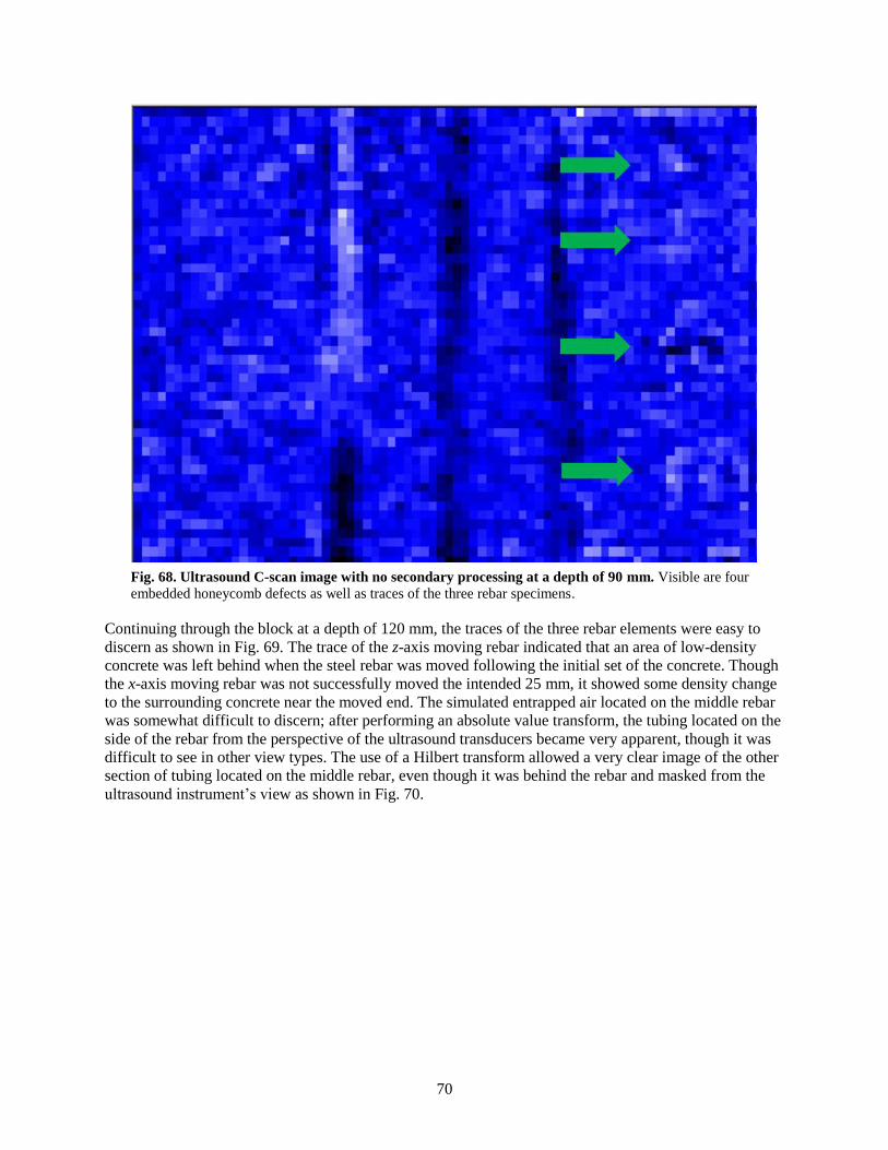
70
Fig. 68. Ultrasound C-scan image with no secondary processing at a depth of 90 mm. Visible are four
embedded honeycomb defects as well as traces of the three rebar specimens.
Continuing through the block at a depth of 120 mm, the traces of the three rebar elements were easy to
discern as shown in Fig. 69. The trace of the z-axis moving rebar indicated that an area of low-density
concrete was left behind when the steel rebar was moved following the initial set of the concrete. Though
the x-axis moving rebar was not successfully moved the intended 25 mm, it showed some density change
to the surrounding concrete near the moved end. The simulated entrapped air located on the middle rebar
was somewhat difficult to discern; after performing an absolute value transform, the tubing located on the
side of the rebar from the perspective of the ultrasound transducers became very apparent, though it was
difficult to see in other view types. The use of a Hilbert transform allowed a very clear image of the other
section of tubing located on the middle rebar, even though it was behind the rebar and masked from the
ultrasound instrument’s view as shown in Fig. 70.

71
Fig. 69. Ultrasound C-scan image at a depth of 120 mm showing damage from
depth-moving rebar (1), lack of rebar reflection due to earlier reflection from
simulated entrapped air (2), and minor concrete disturbance due to length-
moving rebar (3).
Fig. 70. Hilbert transform C-scan ultrasound image at 120 mm depth. Note visibility
of surface-visible pervious prism (left), rebar traces including the masked simulated
delamination (middle), and faint outline of embedded simulated honeycombing
(right).
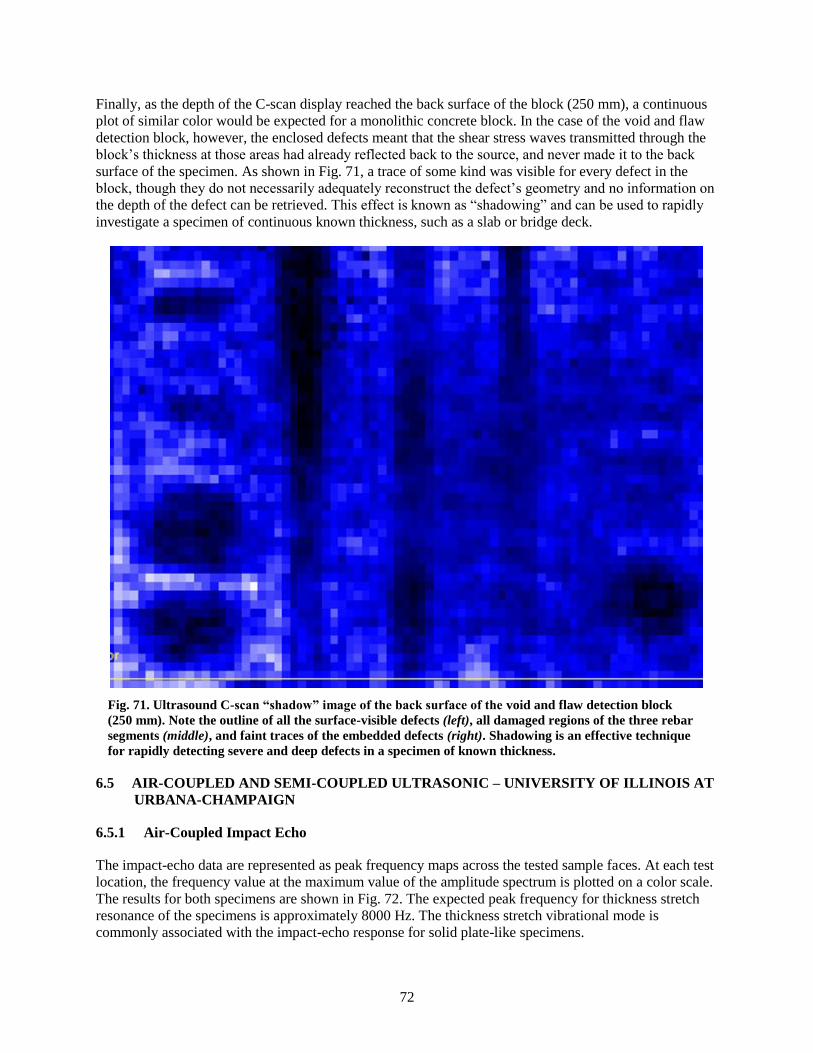
72
Finally, as the depth of the C-scan display reached the back surface of the block (250 mm), a continuous
plot of similar color would be expected for a monolithic concrete block. In the case of the void and flaw
detection block, however, the enclosed defects meant that the shear stress waves transmitted through the
block’s thickness at those areas had already reflected back to the source, and never made it to the back
surface of the specimen. As shown in Fig. 71, a trace of some kind was visible for every defect in the
block, though they do not necessarily adequately reconstruct the defect’s geometry and no information on
the depth of the defect can be retrieved. This effect is known as “shadowing” and can be used to rapidly
investigate a specimen of continuous known thickness, such as a slab or bridge deck.
Fig. 71. Ultrasound C-scan “shadow” image of the back surface of the void and flaw detection block
(250 mm). Note the outline of all the surface-visible defects (left), all damaged regions of the three rebar
segments (middle), and faint traces of the embedded defects (right). Shadowing is an effective technique
for rapidly detecting severe and deep defects in a specimen of known thickness.
6.5 AIR-COUPLED AND SEMI-COUPLED ULTRASONIC – UNIVERSITY OF ILLINOIS AT
URBANA-CHAMPAIGN
6.5.1 Air-Coupled Impact Echo
The impact-echo data are represented as peak frequency maps across the tested sample faces. At each test
location, the frequency value at the maximum value of the amplitude spectrum is plotted on a color scale.
The results for both specimens are shown in Fig. 72. The expected peak frequency for thickness stretch
resonance of the specimens is approximately 8000 Hz. The thickness stretch vibrational mode is
commonly associated with the impact-echo response for solid plate-like specimens.
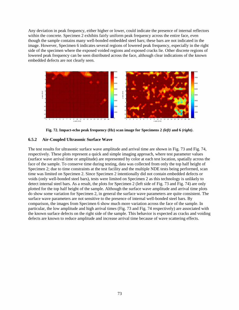
73
Any deviation in peak frequency, either higher or lower, could indicate the presence of internal reflectors
within the concrete. Specimen 2 exhibits fairly uniform peak frequency across the entire face, even
though the sample contains many well-bonded embedded steel bars; these bars are not indicated in the
image. However, Specimen 6 indicates several regions of lowered peak frequency, especially in the right
side of the specimen where the exposed voided regions and exposed cracks lie. Other discrete regions of
lowered peak frequency can be seen distributed across the face, although clear indications of the known
embedded defects are not clearly seen.
Fig. 72. Impact-echo peak frequency (Hz) scan image for Specimens 2 (left) and 6 (right).
6.5.2 Air-Coupled Ultrasonic Surface Wave
The test results for ultrasonic surface wave amplitude and arrival time are shown in Fig. 73 and Fig. 74,
respectively. These plots represent a quick and simple imaging approach, where test parameter values
(surface wave arrival time or amplitude) are represented by color at each test location, spatially across the
face of the sample. To conserve time during testing, data was collected from only the top half height of
Specimen 2; due to time constraints at the test facility and the multiple NDE tests being performed, scan
time was limited on Specimen 2. Since Specimen 2 intentionally did not contain embedded defects or
voids (only well-bonded steel bars), tests were limited on Specimen 2 as this technology is unlikely to
detect internal steel bars. As a result, the plots for Specimen 2 (left side of Fig. 73 and Fig. 74) are only
plotted for the top half height of the sample. Although the surface wave amplitude and arrival time plots
do show some variation for Specimen 2, in general the surface wave parameters are quite consistent. The
surface wave parameters are not sensitive to the presence of internal well-bonded steel bars. By
comparison, the images from Specimen 6 show much more variation across the face of the sample. In
particular, the low amplitude and high arrival times (Fig. 73 and Fig. 74 respectively) are associated with
the known surface defects on the right side of the sample. This behavior is expected as cracks and voiding
defects are known to reduce amplitude and increase arrival time because of wave scattering effects.
x axis (4 in)
y a
xis
(4 in)
1 2 3 4 5 6 7 8 9 10 11 12 13 14 15 16 17 18 19
1
2
3
4
5
6
7
8
9
10
11
12
13 0
1000
2000
3000
4000
5000
6000
7000
8000
x axis (4 in)y a
xis
(4 in)
1 2 3 4 5 6 7 8 9 10 11 12 13 14 15 16 17 18 19
1
2
3
4
5
6
7
8
9
10
11
12
13 0
1000
2000
3000
4000
5000
6000
7000
8000

74
Fig. 73. Ultrasonic surface wave amplitude scan image (volts) for Specimens 2 (left) and 6 (right).
Fig. 74. Ultrasonic surface wave arrival time scan image (seconds) for Specimens 2 (left) and 6 (right).
Note that the surface wave arrival time plot images show good distinction of the individual regions of
defects on the right side of Fig. 74. This is not unexpected because these exposed defects are at the
surface, and intense interaction with the surface waves will occur. The unbonded steel bars in the center
of the sample are not well identified by the surface wave parameters, possibly because the bars are deep
from the surface, outside of the range of the single wavelength depth. However, some high arrival time
indications on the left side of the sample are observed, which are likely associated with the embedded
voided blocks there.
The image on the left side of Fig. 75 is built up of the same dataset as that presented on the right side of
Fig. 74, the only difference being the incorporation of image transparency in the plot. In Fig. 75, the data
in the plots are presented such that the value of time delay is tied to transparency. Higher surface wave
arrival time is associated with increasing opacity (and thus decreasing transparency); the transparency
relation is implemented using the “decrease” option within the “alphamap” function in Matlab in both
plots in Fig. 75. For all plots the “decrease” value is set to 0.4. In the stacked plot in Fig. 75 (right), each
of the signals obtained from the four receiving array sensors are stacked on top of each other in the
vertical sense in the plot. The data in each of the stacked layers are normalized such that the maximum is
always 1.
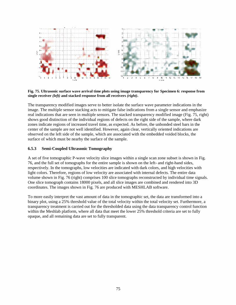
75
Fig. 75. Ultrasonic surface wave arrival time plots using image transparency for Specimen 6: response from
single receiver (left) and stacked response from all receivers (right).
The transparency modified images serve to better isolate the surface wave parameter indications in the
image. The multiple sensor stacking acts to mitigate false indications from a single sensor and emphasize
real indications that are seen in multiple sensors. The stacked transparency modified image (Fig. 75, right)
shows good distinction of the individual regions of defects on the right side of the sample, where dark
zones indicate regions of increased travel time, as expected. As before, the unbonded steel bars in the
center of the sample are not well identified. However, again clear, vertically oriented indications are
observed on the left side of the sample, which are associated with the embedded voided blocks, the
surface of which must be nearby the surface of the sample.
6.5.3 Semi-Coupled Ultrasonic Tomography
A set of five tomographic P-wave velocity slice images within a single scan zone subset is shown in Fig.
76, and the full set of tomographs for the entire sample is shown on the left- and right-hand sides,
respectively. In the tomographs, low velocities are indicated with dark colors, and high velocities with
light colors. Therefore, regions of low velocity are associated with internal defects. The entire data
volume shown in Fig. 76 (right) comprises 100 slice tomographs reconstructed by individual time signals.
One slice tomograph contains 18000 pixels, and all slice images are combined and rendered into 3D
coordinates. The images shown in Fig. 76 are produced with MESHLAB software.
To more easily interpret the vast amount of data in the tomographic set, the data are transformed into a
binary plot, using a 25% threshold value of the total velocity within the total velocity set. Furthermore, a
transparency treatment is carried out for the thresholded data using the data transparency control function
within the Meshlab platform, where all data that meet the lower 25% threshold criteria are set to fully
opaque, and all remaining data are set to fully transparent.
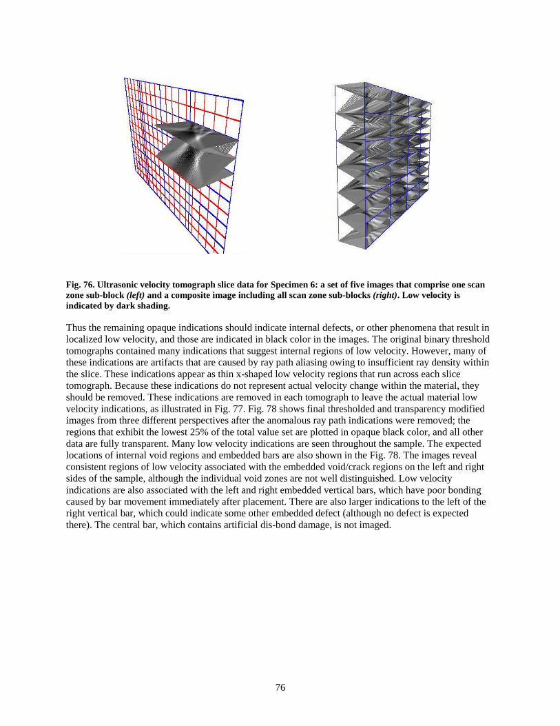
76
Fig. 76. Ultrasonic velocity tomograph slice data for Specimen 6: a set of five images that comprise one scan
zone sub-block (left) and a composite image including all scan zone sub-blocks (right). Low velocity is
indicated by dark shading.
Thus the remaining opaque indications should indicate internal defects, or other phenomena that result in
localized low velocity, and those are indicated in black color in the images. The original binary threshold
tomographs contained many indications that suggest internal regions of low velocity. However, many of
these indications are artifacts that are caused by ray path aliasing owing to insufficient ray density within
the slice. These indications appear as thin x-shaped low velocity regions that run across each slice
tomograph. Because these indications do not represent actual velocity change within the material, they
should be removed. These indications are removed in each tomograph to leave the actual material low
velocity indications, as illustrated in Fig. 77. Fig. 78 shows final thresholded and transparency modified
images from three different perspectives after the anomalous ray path indications were removed; the
regions that exhibit the lowest 25% of the total value set are plotted in opaque black color, and all other
data are fully transparent. Many low velocity indications are seen throughout the sample. The expected
locations of internal void regions and embedded bars are also shown in the Fig. 78. The images reveal
consistent regions of low velocity associated with the embedded void/crack regions on the left and right
sides of the sample, although the individual void zones are not well distinguished. Low velocity
indications are also associated with the left and right embedded vertical bars, which have poor bonding
caused by bar movement immediately after placement. There are also larger indications to the left of the
right vertical bar, which could indicate some other embedded defect (although no defect is expected
there). The central bar, which contains artificial dis-bond damage, is not imaged.

77
Fig. 77. Illustration of procedure to remove ray density artifact indications from thresholded (25%) binary
image plots of tomographic data.
Fig. 78. Thresholded (25%) binary image plots of tomographic data set shown in Fig. 76 for Specimen 6 after
removal of ray path artifacts: top (above left) and front (below left) perspectives with embedded defect
features indicated (below right) and isometric view of the same data.
After erasing ray path artifacts
Before erasing x-shape
1. Original 25% thresholded image
3. Retained indications
2. Artifacts owing to ray path and ray density
Before erasing ray path artifacts

79
7. CONCLUSIONS
7.1 MIRA VERSION 1 – UNIVERSITY OF MINNESOTA
The ultrasonic linear array device, along with processing, analysis, and interpretation conducted by the
University of Minnesota, was shown to be proficient with respect to determining the internal composition
of two concrete specimens fabricated at a Florida Department of Transportation facility (i.e., Specimen 2,
a rebar detection block, and Specimen 6, a void and flaw detection block). Using ultrasonic reconstruction
methods based on Kirchoff migration techniques and associated quantitative measurements, subsurface
characteristics such as reinforcing steel relative size, concrete thickness, irregularities, and inclusion
characterization were determined and reported. These findings were based on the results of an
overlapping grid scanning procedure conducted on two reinforced concrete specimens to simulate realistic
conditions for testing of reinforced concrete containment structures. The testing procedure allowed for
evaluation of extended virtual array reconstructions; overlapping scans were fused to obtain a
tomographic cross section of the structure along both horizontal and vertical dimensions (SAFT-
Panoramic). Interpolation between parallel cross-sectional reconstructions was also conducted to create
three-dimensional reconstructions (SAFT-3D) of the internal characteristics. The use of this technology
for nondestructive evaluation of reinforced concrete containment structures showed promise: examples
include the interpretations for locating inclusions such as reinforcements and for characterizing the
surrounding concrete condition; the identification of poor consolidation and vertical cracks in the
concrete; the differentiation of reinforcement size; and the evaluation of internal concrete conditions
below heavy reinforcement by taking advantage of the spatial diversity of the array system.
While many internal attributes were successfully identified for the specimens tested in this study,
additional verification for different conditions, such as thicker specimens with greater reinforcement
density, should be conducted. While precise results could be achieved when tailoring the testing and
reconstruction procedures to the conditions of this study, the methods should be further refined to address
the conditions of reinforced concrete containment structures. Based on the results of using quantitative
measures for specific internal characteristics such as poor consolidation, future efforts should be focused
on creating quantitative measures rather than relying on qualitative evaluation whenever feasible.
7.2 MIRA VERSION 2 – ENGINEERING & SOFTWARE CONSULTANTS, INC.
MIRA Tomographer, with ultrasonic low frequency technology, was evaluated for its ability to detect
flaws of different kinds (honeycombs, cracks) embedded in thick concrete and also to detect rebar
embedded in concrete at different depths, spacings, and orientations. A two scan approach that included
scanning the specimens vertically and horizontally helped to detect all the embedded objects without any
polarity issues.
MIRA Tomographer successfully detected most of the rebar embedded in Specimen 2 at different
depths, spacings, and orientations. The challenge was with the rebar placed closer together and closer
to the bottom of the slab. As the spacing of the rebar decreased, the noise from the reflections
increased. A smaller horizontal step (<4 in. is currently used) will improve the results. For rebar
placed closer to the bottom of the slab, back wall reflections were a problem. Scanning the back side
of the specimen would eliminate such a problem.
MIRA Tomographer was successfully used to detect the honeycombs and cracks in Specimen 6.
MIRA Tomographer also detected other flaws embedded in Specimen 6 but was not able to
characterize them.

80
7.3 ULTRASONIC LINEAR ARRAY AND GROUND-PENETRAING RADAR –
LYNCH & FERRARO ENGINEERING, INC. (LFE)
Through this series of automated NDE investigations, LFE demonstrated the effectiveness of the
ANTARES system in locating reinforcement, honeycombing, and internal flaws in structural concrete.
The system maximizes its sensitivity through its ability to utilize a variety of NDE techniques and
produce highly dense, repeatable automated scanning grids. It is recommended that the integrated
instruments be further developed to maximize the ANTARES system’s potential to locate deeper, more
difficult-to-find defects for applications such as nuclear containment structures and other massive
structures. The work done in developing the ANTARES system to this point has allowed a significant
amount of versatility to accept new instruments, minimizing the time and effort required for further
development of this sort.
Ground-penetrating radar proved to be fast and accurate in locating the top-layer rebar mats of
Specimen 2, but GPR was unreliable in locating close proximity rebar, secondary layer rebar, and all but
the most severe defects in Specimen 6.
Shear wave ultrasound, while very slow compared to GPR, generated a series of composite images that
located all rebar elements in Specimen 2 except those directly behind the upper layer mats with no
apparent dependency on the orientation of the transducer array. The ultrasound array also successfully
generated a layered image of Specimen 6 that matched the as-built drawings of the blocks at nearly every
detail.
7.4 AIR-COUPLED AND SEMI-COUPLED ULTRASONIC – UNIVERSITY OF ILLINOIS AT
URBANA-CHAMPAIGN
Although the air-coupled impact-echo method is robust and relatively fast to carry out, the peak frequency
image results to do not consistently reveal the presence and location the well-bonded bars in Specimen 2
and the defects in bars and voided regions in Specimen 6. It can be concluded that this method is not
effective for detecting the types of defects and characteristics provided by these concrete specimens. It is
noted that this method is effective for other types of defects, such as shallow and broad delaminations.
The ultrasonic surface wave methods applied here are only able to characterize the layer region near the
surface, to a depth of approximately 5 to 7.5 cm. The method cannot characterize deeper sections.
However, the method was able to identify suspected regions of defects that lie near the surface, such as
the voided concrete blocks. The deeper defects, for example, the poorly bonded steel bars, were not
detected. The arrival time surface wave signal parameter appears to be more effective in detecting and
distinguishing the size of the regions of defects than the surface wave amplitude parameter. Furthermore,
the stacked plot with transparency control provided improved characterization of suspected defect regions
with reduced image artifacts, and this is proposed as the best imaging approach for surface wave data: the
indications seen in this image match well with the expected locations of the voided region, although the
individual voided block are not distinguished in the image.
The semi-coupled through-thickness ultrasonic tomographic method appears to give the best performance
in terms of identifying internal void areas and unbonded embedded bar, when the data are presented in a
thresholded binary image with transparency control. One drawback for this method is the need to correct
the images for ray path artifacts, which can be tedious. Another drawback of the method is the data
collection process, which can be time consuming and labor intensive. However, it can be argued that the
advantages outweigh the drawbacks, as this method is the only one that can penetrate thick structures and
provide good sensitivity to defects and reasonable estimation of location and size. The method was not
able to detect the presence of well-bonded rebar.

81
Finally, it should be noted that the combination of distinct methods, for example, surface wave and
through-thickness tomography, work well to build confidence in the results.
7.5 CONSOLIDATED AND OVERALL CONCLUSIONS
All seven of the nondestructive evaluation techniques that were evaluated performed well on both of the
selected test specimens. Each technique has situations where it performs very well and other situations
where it is somewhat lacking in performance. While the individual merits or shortcoming of each
technique could be discussed, that is not the goal of this research. The goal is to provide a baseline
performance indication of each technique so that better signal processing techniques may be developed to
improve the performance of NDE on thick concrete structures. By taking the data from these tests and
researching advanced signal processing techniques, it is believed that some or all of these techniques can
be made applicable to thick, heavily reinforced concrete structures such as those located in commercial
NPPs. This research into advanced signal processing techniques is expected to continue into FY2014.
While these specimens were the most representative of NPP concrete structures readily available, it is
acknowledged that these specimens are not as representative as they could be since these specimens were
only approximately 10 inches thick. Clearly performing similar tests on thicker specimens would be of
interest to the LWRS NDE program. It is anticipated that a design for one or more thick, heavily
reinforced concrete specimens with flaws and anomalies similar to those of the selected specimens for use
in NDE technique evaluation will be initiated in FY2014.


83
8. REFERENCES
[1] D. A. Clayton and M. S. Hileman, Light Water Reactor Sustainability Non-Destructive Evaluation
for Concrete Research and Development Roadmap, ORNL/TM-2012/360, Oak Ridge National
Laboratory, 2012.
[2] D. A. Clayton and C. M. Smith, Summary of Large Concrete Samples, ORNL/TM-2013/223, Oak
Ridge National Laboratory, 2013.
[3] D. Algernon, D. Hiltunen, and C. Ferraro, "Validation of Nondestructive Testing Equipmnet for
Concrete," University of Florida Department of Civil and Coastal Engineering, 2010.
[4] K. Hoegh, L. Khazanovich, and H. T. Yu, "Ultrasonice Tomography for Evaluation of Concrete
Pavements," Transportation Resarch Record: Journal of the Transportation Research Board, vol.
2232, pp. 85–94, 2011.
[5] K. Hoegh, L. Khazanovich, K. R. Maser, and N. Tran, "Evaluation of Ultrasonice Technique for
Detecting Delamination in Asphalt Pavements," in Transportation Research Board 91st Annual
Meeting, McLean, 2012a.
[6] K. Hoegh, L. Khazanovich, and T. Yu, "Concrete Pavement Joint Diagnostics Using Ultrasonic
Tomography," in Transportation Research Board 91st Annual Meeting, 2012.
[7] K. Hoegh and L. Khazanovich, "Correlation Analysis of 2D Tomographic images for Flaw
Detection in Pavement," ASTM International Journal of Testing and Evaluation, vol. 40, no. 2,
March 2012.
[8] T. Oh, J. Popovics, S. Ham, and S. Shin, "Improved Interpretation of Vibation Responses from
Concrete Delamination Defects Using Air-Coupled Impact Resonance Tests," J. Eng. Mech., vol.
139, pp. 315–324, 2013.
[9] D. King, "Collapse Dynamics of Ultrasound Contrast Agent Microbubbles," University of Illinois
at Urbana-Champaign, 2012.
[10] K. Hall, "Air-coupled Ultrasonic Tomographic Imaging of Concrete Elements," University of
Illinois at Urbana-Champaign, 2011.
[11] S. L. Hahn, Hilbert Transforms in Signal Processing, Boston: Artech House, 1996.
[12] N. E. Huang and N. O. Attoh-Okine, The Hilbert-Huang Transform in Engineering, CRC, 2005.
[13] F. R. Kschischang, The Hilbert Transform, University of Toronto, 2006.
[14] G. Todoran, R. Holonec, and C. Iakab, Discrete Hilbert Transform. Numeric Algorithms., 2008.
[15] L. Marple, Jr., "Computing the Discrete-time 'Analytic' Signal via FFT," IEEE Transactions on
Signal Processing, vol. 47, pp. 2600–2603, 1999.
[16] B. Gold, A. V. Oppenheim, and C. M. Rader, "Theory and Implementation of the Discrete Hilbert
Transform," in Proceedings of the Symposium on Computer Processing in Communications, New
York, 1970.
[17] A. V. Oppenheim, R. W. Schafer, and J. R. Buck, Discrete-time Signal Processing, Englewood
Cliffs, NJ: Prentice Hall, 1989.
[18] F. Schubert and B. Koehler, "Three-Dimensional Time Domain Modeling of Ultrasonic Wave
Propagation in Concrete in Explicit Consideration of Aggregates and Porosity," Journal of
Computational Acoustics, pp. 1543–1560, 2001.
[19] Federal Highway Administration NDE Validation Center, "Non-Destructive Inspection Protocol for
Reinforced Concrete Highway Barriers and Bridge Railings," McLean, VA, 2013.
[20] Florida Department of Transportation Research Center and University of Florida Department of
Civil and Coastal Engineering, "Validation of Nondestructive Testing Equipment for Concrete -
Final Report," Gainesville, FL, 2011.
[21] K. Hoegh, T. Yu, and L. Khazanovich, "Magnetic imaging tools scanner (MIT Scan-2) application
in Notrh America: five years later," in 9th International Conference on Concrete Pavements, 2008.


APPENDIX A. INTERPRETATION AND ANALYSIS OF ULTRASONIC
LINEAR ARRAY SIGNALS


A-3
APPENDIX A. INTERPRETATION AND ANALYSIS OF ULTRASONIC LINEAR ARRAY
SIGNALS
This appendix describes the development of various reconstruction procedures for interpretation of the
ultrasonic linear array signals. In addition, several application specific automation procedures were
developed to increase productivity and accuracy in interpretation of a large number of reconstructions.
A.1 RECONSTRUCTION
Typical synthetic aperture radar (SAR) and synthetic aperture focusing technique (SAFT) formulations
are applied for interpretation of multiple signals with sending and receiving transducers at the same
location. These formulations need to be generalized for interpretation of signals with sending and
receiving transducers located at different locations for application with MIRA. In this case a signal sent
from one location but received at various locations along the surface should be accounted for in this
formulation.
Similar to the formulation for point source emission and reception at a single location, the region of
interest (ROI) below the testing aperture can be treated as a collection of point targets. The fundamental
expression for SAR is generalized for each emitting and receiving transducer pair positioned at and
,
respectively, and can be represented as shown in equation [A.1]:
(
) ∫ ∫ ( ) ( (
))
[A.1]
where (
) is the received impulse due to emitted impulse ( (
)); ( ) is the
reflectivity function of the ROI; and are the horizontal and vertical positions in the ROI, respectively;
and is defined by the following relationship:
(√ ( )
√ ( ) ) [A.2]
The impulse response received at the surface as a function of time, (
), is a combination of
reflections from each position below the measurement as defined by the reflectivity function, ( ). This function depends on the reflection coefficient of each of the potential point targets in the ROI which
is a function of changes in modulus and density. Since the reflection coefficients are determined by
changes in acoustic impedance characteristics and thus contain the information about material changes in
stiffness or density, this is the information of interest when creating the reconstruction images. Fig. 79
shows a representation of potential contributing point sources for a single intensity value within
( ) according to the fundamental SAR equation.

A-4
Fig. 79. Representation of potential contributing point sources at a constant time (Roundtrip) from the
emitting/receiving transducer according to the fundamental expression.
A.2 SAFT B-SCAN
The synthetic aperture focusing technique can be used for the ultrasonic linear array used in this study in a
similar manner to that described for single sending and receiving pairs. To allow for integration over the
various transducer locations, ∫ ∫
, the impulses received at the surface versus time can be
expressed in terms of distances. This can be accomplished by assuming a constant shear wave velocity,
, determined from equation A.1. If the signals are emitted within interval [
] and
received within interval [
], the reconstructed image at each point ( ) can be obtained by
integrating over all possible transducer pair (impulse emit and receive) locations:
( ) ∫ ∫ (
) (
(√ (
) √ ( ) ))
[A.3]
where (
) is the apodization factor that is typically a function of the distance traveled, incident
angle, and/or divergence of the reflection point location with respect to the emitted/received signal.
The measured signals for the setup in this study have transducer locations at spacing
. Fig. 80 shows an example linear array setup with being the leftmost transducer. For the
ultrasonic linear array used in this study, the leftmost emitting transducer is located at the leftmost
transducer location,
, leftmost receiving transducer is located adjacent to the leftmost emitting
transducer
, rightmost receiving transducer is located at the rightmost transducer
location
, and rightmost emitting transducer is located adjacent to the rightmost receiving
transducer location
.
Region of Interest (ROI)
x
z

A-5
Fig. 80. Linear array representation.
After applying the shift factor to account for system delay the reconstructed image is obtained at discrete
points by summing over all possible transducer pair locations using the following relationship for the
ultrasonic linear array:
∑ ∑ ( ) ( )
[A.4]
where
( ) (
(√
( ) √
( ) )) [A.5]
where is the image reflectivity assigned to each position within the ROI, is the number of
transducer locations, and are the indexes for the emitting and receiving transducers, and and are
the indexes for the horizontal and vertical positions of the ROI.
If the ROI has W indexes in the horizontal direction and D indexes in the vertical direction, the following
matrix formalization can be used to represent SAFT reconstructed image, [ ]:
[A.6]
Target (
…. ….
…. …. …. ….
…. …. …. ….
…. …. …. …. ….
…. ….
=

A-6
The apodization factor accounts for incident angle and other traits of the signal and tested medium. For
the ultrasonic linear array used in this study for testing of concrete, the apodization factor given in
equation A.7 was used:
(
) ( ) (
). [A.7]
Where
( )
√( )
( )
√( )
An example of typical data from the ultrasonic linear array on a reinforced concrete pavement (CRCP) is
given herein. Fig. 81 shows a schematic of the CRCP structure at the example scan location. It can be
observed that there is a set of three longitudinal reinforcements represented by black circles in the
schematic within the ROI where the measurement was taken.
Fig. 81. Schematic of the CRCP subsurface at the example scan location.
Fig. 82 shows three example impulse responses, ( ) ( ) ( ) of the total 45 emitting and
receiving pairs comprising the example scan. It can be observed that there are peaks in amplitude at
certain locations within the time histories in addition to the direct arrival positions. While these spikes in
amplitude are associated with reflectivity within the ROI, such as reinforcements and layer boundaries,
the location of the cause of these reflections are difficult to interpret.
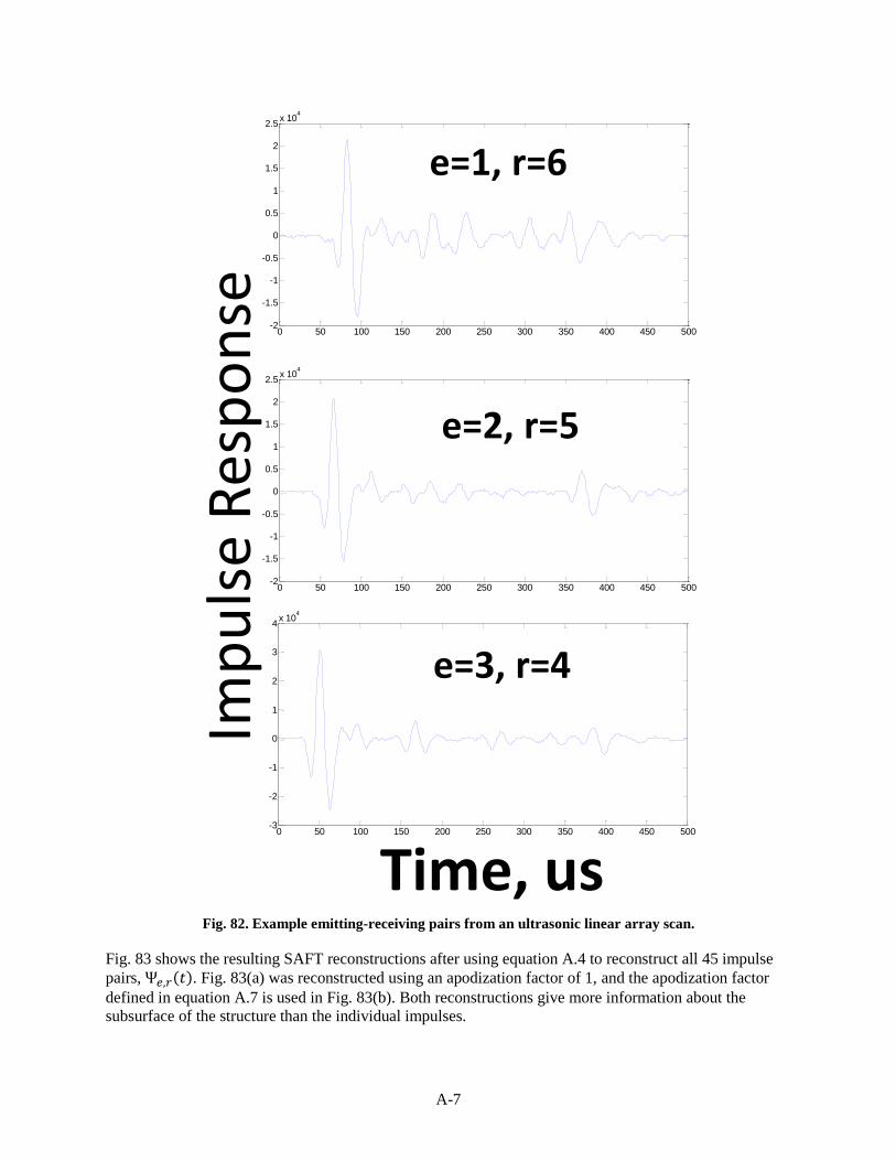
A-7
Fig. 82. Example emitting-receiving pairs from an ultrasonic linear array scan.
Fig. 83 shows the resulting SAFT reconstructions after using equation A.4 to reconstruct all 45 impulse
pairs, ( ). Fig. 83(a) was reconstructed using an apodization factor of 1, and the apodization factor
defined in equation A.7 is used in Fig. 83(b). Both reconstructions give more information about the
subsurface of the structure than the individual impulses.
0 50 100 150 200 250 300 350 400 450 500-2
-1.5
-1
-0.5
0
0.5
1
1.5
2
2.5x 10
4
e=1, r=6
0 50 100 150 200 250 300 350 400 450 500-2
-1.5
-1
-0.5
0
0.5
1
1.5
2
2.5x 10
4
e=2, r=5
0 50 100 150 200 250 300 350 400 450 500-3
-2
-1
0
1
2
3
4x 10
4
e=3, r=4
Imp
uls
e R
esp
on
se
Time, us

A-8
The high reflectivity locations in the SAFT reconstructions indicate the location of changes in acoustic
impedance such as the reinforcements and the layer boundary. It can also be observed that the structural
noise observed in Fig. 83 (a) in the sound concrete portions is not present in Fig. 83(b). This illustrates
that the use of the apodization factor defined in equation A.7 improves the focusing capabilities of the
SAFT reconstruction and eliminates some of the structural noise such as direct arrival intensities that do
not represent the reflectivity of the ROI.
Fig. 83. Example SAFT reconstruction with the apodization factor equal to (a) 1 and (b) defined by equation
A.7.
2009-09-2910
20
pos17
Transverse Width, inches
Depth
, in
ches
5 10 16
0
7
13
20
(a)
(b)

A-9
A.3 INSTANTANEOUS AMPLITUDE SAFT B-SCAN (SAFT-IA)
In most cases, the reconstruction analysis for concrete pavement applications is concentrated on
identifying the source of the changes in acoustic impedance in the subsurface. Further focusing of the
reconstruction can be achieved by analyzing changes in instantaneous amplitude within the ROI. The
Hilbert transform is useful in calculating instantaneous attributes of a time series, especially the amplitude
and frequency [11] [12] [13] [14] [15] [16] [17]. The Hilbert transform, ( ), of a given function, ( ), is
defined by the following equation:
( )
∫
( )
[A. ]
where is the principal value of the singular integral in equation A.8.
And the complex analytic signal, ( ), is given by:
( ) ( ) ( ) [A. ]
Since the reconstruction analysis in this study is based on focusing high reflectivity (changes in acoustic
impedance) within the ROI with high magnitude pulse amplitudes, calculation of instantaneous
amplitudes during the SAFT analysis can give higher resolution reconstructions. Since the Hilbert
Transform envelope will be used during the reconstruction process, a slight change in the determination
of the shift factor must be applied. Equation A.10 is used to calculate the instantaneous amplitude of each
individual transducer pair impulse time history.
( ) √( ( ))
(
∫
( )
)
[A. ]
where ( ) defines the instantaneous amplitude envelope of time history pair, ( ), and is the
principal value of the singular integral in equation A.10.
Use of the instantaneous amplitude, ( ), permits a modification of equation 2.15, which was based on
the raw impulse time-history signal. The instantaneous amplitude-based shift factor, , for each
signal is given in equation A.11:
∑ ∑
[A. ]
where is the time of flight to the maximum instantaneous amplitude of each
. Fig. 84 shows
the same example transducer pair impulse response, , and corresponding instantaneous amplitude
envelope, , illustrating the process of obtaining
(bottom).

A-10
Fig. 84. Determination of the direct arrival peak using the instantaneous amplitude
envelope.
The full-waveform impulse responses are corrected by setting for each sending and
receiving pair before it is applied to the SAFT-IA B-scan reconstruction.
Similarly, for the ultrasonic linear array SAFT reconstructions based on the Hilbert transform, we are
interested focusing the instantaneous amplitude within the ROI to changes in acoustic impedance.
Therefore, the Hilbert transform is performed for each horizontal coordinate SAFT reconstruction in a
similar manner to equation A.10 as follows:
( ) √( ( )) (
∫
( )
) [A.12]
where ( ) defines the instantaneous amplitude-based SAFT reconstruction and is the principal
value of the singular integral in equation A.12. If the ROI is represented by a set of points located
in columns, equally spaced in the horizontal direction, and rows equally spaced in the vertical
direction, the following matrix formalization can be used to represent SAFT-IA reconstructed
image,[ ]
:
0 50 100 150 200 250 300 350 400 450 500-2
-1.5
-1
-0.5
0
0.5
1
1.5
2
2.5x 10
4
0 50 100 150 200 250 300 350 400 450 5000
0.5
1
1.5
2
2.5x 10
4
Imp
uls
e R
esp
on
seIn
stan
tan
eo
us
Am
plit
ud
e
Time, us
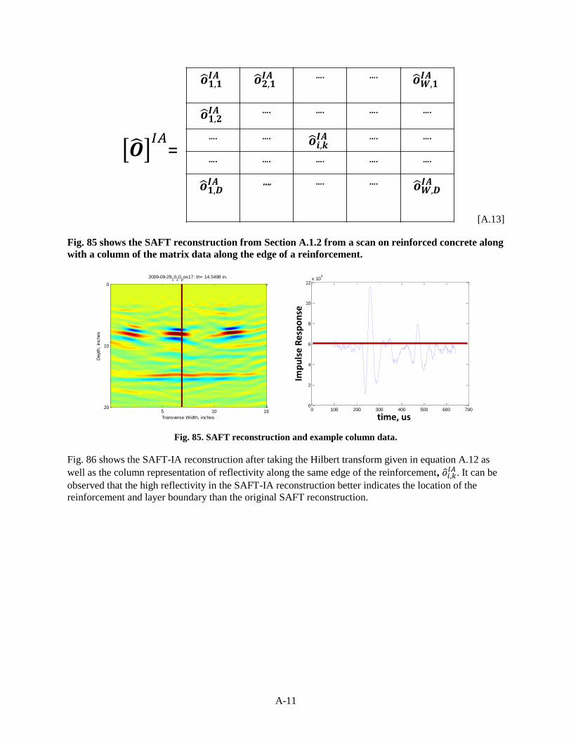
A-11
[A.13]
Fig. 85 shows the SAFT reconstruction from Section A.1.2 from a scan on reinforced concrete along
with a column of the matrix data along the edge of a reinforcement.
Fig. 85. SAFT reconstruction and example column data.
Fig. 86 shows the SAFT-IA reconstruction after taking the Hilbert transform given in equation A.12 as
well as the column representation of reflectivity along the same edge of the reinforcement, . It can be
observed that the high reflectivity in the SAFT-IA reconstruction better indicates the location of the
reinforcement and layer boundary than the original SAFT reconstruction.
…. ….
…. …. …. ….
…. …. …. ….
…. …. …. …. ….
…. ….
=
0 100 200 300 400 500 600 7000
2
4
6
8
10
12x 10
42009-09-2910
20
pos17: th= 14.5498 in.
Transverse Width, inches
Depth
, in
ches
5 10 16
0
10
20
time, us
Imp
uls
e R
esp
on
se

A-12
Fig. 86. SAFT-IA reconstruction and example column data.
Furthermore, the use of the Matlabtm
two dimensional smoothing function (‘disk’ filtering) allows for
additional elimination of structural noise in the reconstruction. Fig. 87 illustrates the resulting filtered
SAFT-IA B-scan of the forensic verification of the reinforcement location. It can be observed that the
depth of the reinforcement corresponds to the higher instantaneous amplitude region within the SAFT-IA
B-scan reconstruction.
Fig. 87. Forensic verification of the focused reinforcement location within the SAFT-IA B-scan.
0 100 200 300 400 500 600 7000
1
2
3
4
5
6x 10
42009-09-2910
20
pos17: th= 15.0389 in.
Transverse Width, inches
Depth
, in
ches
5 10 16
0
10
20
time, us
Inst
anta
neo
us
Am
plit
ud
e
2009-09-2910
20
pos17
Transverse Width, inches
Depth, in
ches
5 10 16
0
7
13
20
Cored Reinforcement Position

A-13
A.4 SAFT-3D
Three-dimensional reconstruction of subsurface characteristics can simplify interpretation of multiple
ultrasonic array scans. SAFT 3-dimensional reconstructions (SAFT-3D) can be achieved using various
interpolation and filtering techniques. Fig. 88 shows the SAFT-IA B-scan from Fig. 87 as well as ten
additional measurements at 50 mm step sizes in the longitudinal direction.
Fig. 88. SAFT-IA B-scans from the cored location as well as 10 subsequent scans in the
longitudinal direction.
These scans were used to create the remaining length of the cored reinforcement as well as the
reinforcement to the right of the cored reinforcement in a three-dimensional reconstruction (SAFT-3D).
Fig. 89 shows a schematic of the SAFT-3D reconstruction process where scans are taken in step sizes in
the longitudinal direction and interpolation techniques are used to create the continuous 3D image of the
ROI. The process of creating the SAFT-3D reconstruction included selecting an optimal threshold, using
the same ‘disk’ filtering function for each SAFT-IA B-scan, a MATLABTM
3D matrix smoothing function

A-14
(‘smooth3’), and a MATLABTM
interpolation function (‘isosurface’) within the volume of the
reconstruction.
Fig. 89. Schematic representation of the process of creating SAFT-3D reconstructions.
The SAFT-3D reconstruction of 300 mm of depth within the concrete layer of a 500 mm longitudinal
(850 mm to 1350 mm) by 400 mm transverse location is given in Fig. 90. The reinforcement on the left
side at 850 mm in the longitudinal direction corresponds to the cored location. This type of SAFT 3D
reconstruction can be useful for getting relational information about the high intensity reflections to
determine if the reflection is caused by an as designed inclusion or damaged concrete.
Fig. 90. SAFT 3D reconstruction using the SAFT-IA B-scan
reconstructions shown in Fig. 88.
Transverse direction
Dep
th d
irec
tio
n
Longitudinal Reinforcement
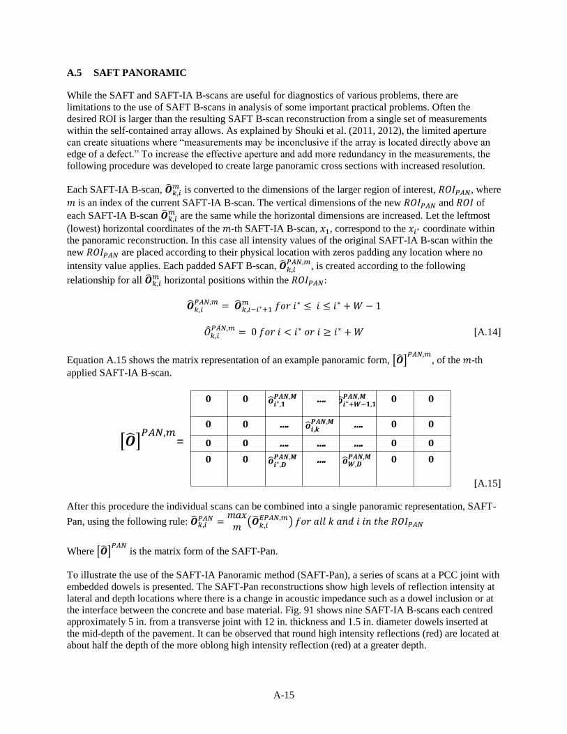
A-15
A.5 SAFT PANORAMIC
While the SAFT and SAFT-IA B-scans are useful for diagnostics of various problems, there are
limitations to the use of SAFT B-scans in analysis of some important practical problems. Often the
desired ROI is larger than the resulting SAFT B-scan reconstruction from a single set of measurements
within the self-contained array allows. As explained by Shouki et al. (2011, 2012), the limited aperture
can create situations where “measurements may be inconclusive if the array is located directly above an
edge of a defect.” To increase the effective aperture and add more redundancy in the measurements, the
following procedure was developed to create large panoramic cross sections with increased resolution.
Each SAFT-IA B-scan, is converted to the dimensions of the larger region of interest, , where
is an index of the current SAFT-IA B-scan. The vertical dimensions of the new and of
each SAFT-IA B-scan are the same while the horizontal dimensions are increased. Let the leftmost
(lowest) horizontal coordinates of the -th SAFT-IA B-scan, , correspond to the coordinate within
the panoramic reconstruction. In this case all intensity values of the original SAFT-IA B-scan within the
new are placed according to their physical location with zeros padding any location where no
intensity value applies. Each padded SAFT B-scan,
, is created according to the following
relationship for all horizontal positions within the
[A.14]
Equation A.15 shows the matrix representation of an example panoramic form, [ ]
, of the -th
applied SAFT-IA B-scan.
[A.15]
After this procedure the individual scans can be combined into a single panoramic representation, SAFT-
Pan, using the following rule:
( )
Where [ ]
is the matrix form of the SAFT-Pan.
To illustrate the use of the SAFT-IA Panoramic method (SAFT-Pan), a series of scans at a PCC joint with
embedded dowels is presented. The SAFT-Pan reconstructions show high levels of reflection intensity at
lateral and depth locations where there is a change in acoustic impedance such as a dowel inclusion or at
the interface between the concrete and base material. Fig. 91 shows nine SAFT-IA B-scans each centred
approximately 5 in. from a transverse joint with 12 in. thickness and 1.5 in. diameter dowels inserted at
the mid-depth of the pavement. It can be observed that round high intensity reflections (red) are located at
about half the depth of the more oblong high intensity reflection (red) at a greater depth.
=
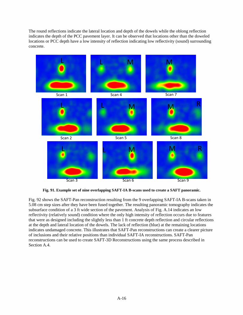
A-16
The round reflections indicate the lateral location and depth of the dowels while the oblong reflection
indicates the depth of the PCC pavement layer. It can be observed that locations other than the doweled
locations or PCC depth have a low intensity of reflection indicating low reflectivity (sound) surrounding
concrete.
Fig. 91. Example set of nine overlapping SAFT-IA B-scans used to create a SAFT panoramic.
Fig. 92 shows the SAFT-Pan reconstruction resulting from the 9 overlapping SAFT-IA B-scans taken in
5.08 cm step sizes after they have been fused together. The resulting panoramic tomography indicates the
subsurface condition of a 3 ft wide section of the pavement. Analysis of Fig. A.14 indicates an low
reflectivity (relatively sound) condition where the only high intensity of reflection occurs due to features
that were as designed including the slightly less than 1 ft concrete depth reflection and circular reflections
at the depth and lateral location of the dowels. The lack of reflection (blue) at the remaining locations
indicates undamaged concrete. This illustrates that SAFT-Pan reconstructions can create a clearer picture
of inclusions and their relative positions than individual SAFT-IA reconstructions. SAFT-Pan
reconstructions can be used to create SAFT-3D Reconstructions using the same process described in
Section A.4.
L M R
L
L
L
L
L M
M
M
M
M
R
Scan 1
Scan 2
Scan 4 Scan 7
Scan 8Scan 5
Scan 9Scan 3 Scan 6
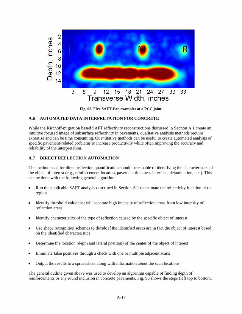
A-17
Fig. 92. Five SAFT-Pan examples at a PCC joint.
A.6 AUTOMATED DATA INTERPRETATION FOR CONCRETE
While the Kirchoff-migration based SAFT reflectivity reconstructions discussed in Section A.1 create an
intuitive focused image of subsurface reflectivity in pavements, qualitative analysis methods require
expertise and can be time consuming. Quantitative methods can be useful to create automated analysis of
specific pavement-related problems to increase productivity while often improving the accuracy and
reliability of the interpretation.
A.7 DIRECT REFLECTION AUTOMATION
The method used for direct reflection quantification should be capable of identifying the characteristics of
the object of interest (e.g., reinforcement location, pavement thickness interface, delamination, etc.). This
can be done with the following general algorithm:
Run the applicable SAFT analysis described in Section A.1 to estimate the reflectivity function of the
region
Identify threshold value that will separate high intensity of reflection areas from low intensity of
reflection areas
Identify characteristics of the type of reflection caused by the specific object of interest
Use shape recognition schemes to decide if the identified areas are in fact the object of interest based
on the identified characteristics
Determine the location (depth and lateral position) of the center of the object of interest
Eliminate false positives through a check with one or multiple adjacent scans
Output the results to a spreadsheet along with information about the scan locations
The general outline given above was used to develop an algorithm capable of finding depth of
reinforcements or any round inclusion in concrete pavements. Fig. 93 shows the steps (left top to bottom,
L M R
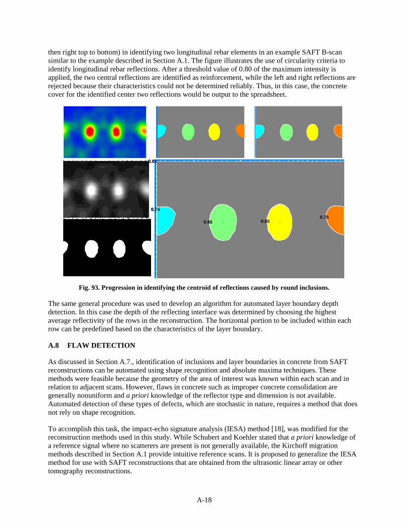
A-18
then right top to bottom) in identifying two longitudinal rebar elements in an example SAFT B-scan
similar to the example described in Section A.1. The figure illustrates the use of circularity criteria to
identify longitudinal rebar reflections. After a threshold value of 0.80 of the maximum intensity is
applied, the two central reflections are identified as reinforcement, while the left and right reflections are
rejected because their characteristics could not be determined reliably. Thus, in this case, the concrete
cover for the identified center two reflections would be output to the spreadsheet.
Fig. 93. Progression in identifying the centroid of reflections caused by round inclusions.
The same general procedure was used to develop an algorithm for automated layer boundary depth
detection. In this case the depth of the reflecting interface was determined by choosing the highest
average reflectivity of the rows in the reconstruction. The horizontal portion to be included within each
row can be predefined based on the characteristics of the layer boundary.
A.8 FLAW DETECTION
As discussed in Section A.7., identification of inclusions and layer boundaries in concrete from SAFT
reconstructions can be automated using shape recognition and absolute maxima techniques. These
methods were feasible because the geometry of the area of interest was known within each scan and in
relation to adjacent scans. However, flaws in concrete such as improper concrete consolidation are
generally nonuniform and a priori knowledge of the reflector type and dimension is not available.
Automated detection of these types of defects, which are stochastic in nature, requires a method that does
not rely on shape recognition.
To accomplish this task, the impact-echo signature analysis (IESA) method [18], was modified for the
reconstruction methods used in this study. While Schubert and Koehler stated that a priori knowledge of
a reference signal where no scatterers are present is not generally available, the Kirchoff migration
methods described in Section A.1 provide intuitive reference scans. It is proposed to generalize the IESA
method for use with SAFT reconstructions that are obtained from the ultrasonic linear array or other
tomography reconstructions.
0.01
0.84
0.80 0.85
0.01
0.74
0.86 0.850.75
0.01
0.74
0.86 0.850.75

A-19
This can be accomplished by generalizing the IESA into a two dimensional ultrasonic tomography
signature analysis method (2D-UTSA or UTSA). Pearson’s correlation coefficient is adapted for
comparison of reconstructed intensity matrices as follows using the SAFT-IA B-scan variables introduced
in Section A.1.2:
[[ ] [ ] ]
√ [[ ] ] [[ ] ]
∑ ∑ (
)(
)
∑ ∑ (
)
∑ ∑ (
)
[A.16]
where [ ]
and [ ]
are the matrices of reflection intensity for the reference SAFT-IA B-scan and
m-th SAFT-IA B-scan, respectively;
and are the single intensity values of the reference signal
and m-th reconstruction, respectively, with depth below the measurement location increasing with and
the location along the horizontal direction of the scan increasing with ;
and are the mean
intensities of the reference scan and m-th scan, respectively; and are the number of width and depth
intensity values in the depth and device aperture direction, respectively; and is Pearson’s
correlation coefficient, which measures the strength of the linear dependence between [ ]
and
[ ]
.
Thus, if a SAFT-IA B-scan taken on relatively sound concrete with similar structural geometry is used as
the reference scan, flawed concrete locations can be identified. On the extremes, a value of 0 would
indicate no correlation and a value of 1 would indicate that the two SAFT-IA B-scans are related
linearly. Therefore, a higher would indicate that the m-th SAFF-IA B-scan was taken on sound
concrete, and a significant decrease in the correlation coefficient would indicate nonuniform SAFT-IA B-
scans, or flawed concrete, especially if observed in a group of adjacent scans. This type of analysis will be
referred to as the 2D-UTSA method.
In addition to making the method applicable for the type of data gathered by the study, the use of the
expanded Pearson’s correlation for 2D comparison improves the method by correcting the issues of the
IESA technique in selecting the reference signal. As explained in Section A.1.2 the SAFT-IA
reconstruction creates a relatively intuitive reconstructed image of the ROI reflectivity function.
Therefore, selection of a damage free reference scans is possible based on past experience with signal
interpretation of SAFT reconstructions [4] [7] [6] and the misinterpretations associated with the IESA
method can be mitigated. When necessary, coring should be conducted to verify that the reference scan is
indeed damage free.
Furthermore, subsurface damage in concrete is generally entropic in that there is little variation between
SAFT-IA B-scans of concrete in relatively good condition at different locations if the same instrument
settings are used, while there is a significant variation between scans where flaws are present at different
locations. Therefore, sound concrete will have similar levels of correlation with the reference SAFT-IA
B-scan, whereas the correlation of scans with flaws at different locations will fluctuate. Therefore, a
procedure where the reference scan is taken as the average of all of the SAFT-IA B-scans in the set is
introduced. It is expected that sound concrete may not necessarily have as high of a correlation with the
generated reference scan as is the case for a manually selected reference scan. However, if a significant
portion of measurements are made on sound concrete, the sound concrete locations should result in
similar correlation values, while unsound concrete will result in lower values due to the randomness of
flaws. Thus, decreases are still present in the correlogram even when the reference scan includes
contributions from the flawed concrete locations. This method is not overly sensitive to selection of the
reference scan, and can be generally applied to locate areas of flawed concrete.
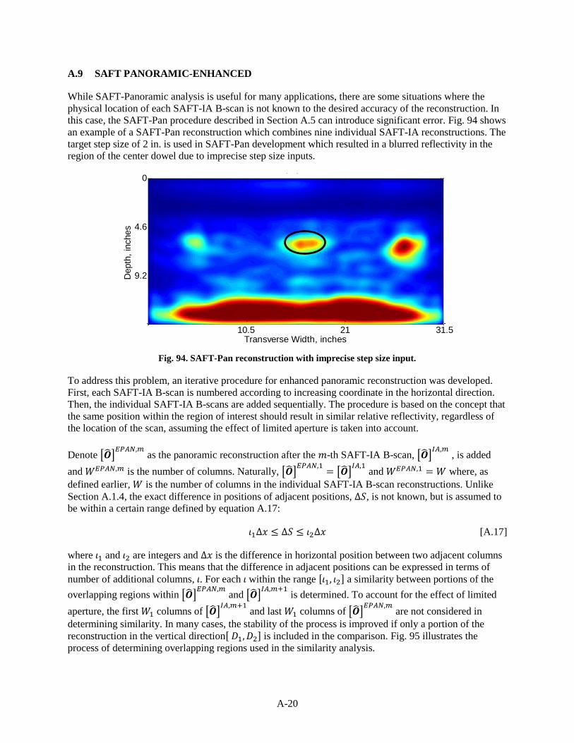
A-20
A.9 SAFT PANORAMIC-ENHANCED
While SAFT-Panoramic analysis is useful for many applications, there are some situations where the
physical location of each SAFT-IA B-scan is not known to the desired accuracy of the reconstruction. In
this case, the SAFT-Pan procedure described in Section A.5 can introduce significant error. Fig. 94 shows
an example of a SAFT-Pan reconstruction which combines nine individual SAFT-IA reconstructions. The
target step size of 2 in. is used in SAFT-Pan development which resulted in a blurred reflectivity in the
region of the center dowel due to imprecise step size inputs.
Fig. 94. SAFT-Pan reconstruction with imprecise step size input.
To address this problem, an iterative procedure for enhanced panoramic reconstruction was developed.
First, each SAFT-IA B-scan is numbered according to increasing coordinate in the horizontal direction.
Then, the individual SAFT-IA B-scans are added sequentially. The procedure is based on the concept that
the same position within the region of interest should result in similar relative reflectivity, regardless of
the location of the scan, assuming the effect of limited aperture is taken into account.
Denote [ ]
as the panoramic reconstruction after the -th SAFT-IA B-scan, [ ]
, is added
and is the number of columns. Naturally, [ ]
[ ]
and where, as
defined earlier, is the number of columns in the individual SAFT-IA B-scan reconstructions. Unlike
Section A.1.4, the exact difference in positions of adjacent positions, , is not known, but is assumed to
be within a certain range defined by equation A.17:
[A.17]
where and are integers and is the difference in horizontal position between two adjacent columns
in the reconstruction. This means that the difference in adjacent positions can be expressed in terms of
number of additional columns, . For each within the range [ ] a similarity between portions of the
overlapping regions within [ ]
and [ ]
is determined. To account for the effect of limited
aperture, the first columns of [ ]
and last columns of [ ]
are not considered in
determining similarity. In many cases, the stability of the process is improved if only a portion of the
reconstruction in the vertical direction[ ] is included in the comparison. Fig. 95 illustrates the
process of determining overlapping regions used in the similarity analysis.
pos9pan
Transverse Width, inches
Depth
, in
ches
10.5 21 31.5
0
4.6
9.2
pos9pan
Transverse Width, inches
Depth
, in
ches
9.2 18.5 27.7
0
4.6
9.2

A-21
Fig. 95. Determination of overlapping regions between the reconstructions and determination of the next
panoramic reconstruction
The degree of similarity of the overlapping regions, ( ), is determined based on Pearson’s Correlation as
follows:
( ) ∑ ∑ (
)(
)
∑ ∑ (
)
∑ ∑ (
)
[A.18]
where
∑ ∑
( )( )
∑ ∑
( )( )
The that results in the maximum value of function ( ) on the interval [ ] is denoted as the optimal
shift factor, . Then the next SAFT-EPAN reconstruction, [ ]
, is defined as follows:

A-22
[A.19]
(
)
for
and
for ,
where is the width of the new SAFT-EPAN as defined:
.
Each subsequent SAFT panoramic reconstruction, [ ]
, is obtained from addition of [ ]
and the next SAFT-IA B-scan, [ ]
. The additional number of columns in the new reconstruction,
, is determined by comparing the similarity between portions of the overlapping regions within
[ ]
and [ ]
. The additional columns, , are chosen from within the range of potential shift
factors [ ].
Fig. 96 illustrates the similarity of overlapping scans as a function of possible shift factors, ( ), used for
fusing of the nine scans from this example. The plot is given on an x-axis scale where columns are
converted to inches and the target shift factor of 2 in. is marked by the black vertical line. The column
range, [ ] used for determination of the optimal shift factor, , is equivalent to a range of 1.4 in. to 2.6
in. It can be observed that the optimal step sizes, as determined by the resulting in the peak of the ( ) curves, are significantly different than the target shift factor at various locations. Smaller than target shift
factors, , were used for placement of SAFT-IA scans, [ ]
, while larger than target shift
factors, , were used for placement of SAFT-IA scans, [ ]
into each iterative
formulation of the SAFT-Epan, [ ]
.

A-23
Fig. 96. Similarity of overlapping region curves used for placement of SAFT-IA
reconstructions into the SAFT-EPan reconstruction.
Fig. 97 shows the (a) original SAFT-Pan reconstruction and (b) SAFT-EPan reconstruction both obtained
from the same nine individual SAFT-IA scans in this example. It can be observed that the blurry oblong
reflection at the center dowel in the SAFT-Pan is a more focused circular reflection when using the
SAFT-EPan reconstruction. Correcting for some of the uncertainty in the measurement process by placing
the scans based on similarity of overlapping regions allows for a more focused reconstruction that is
consistent with the reflectivity in the region.
m=2
m=3
m=4
m=5
m=6
m=7
m=8
m=9
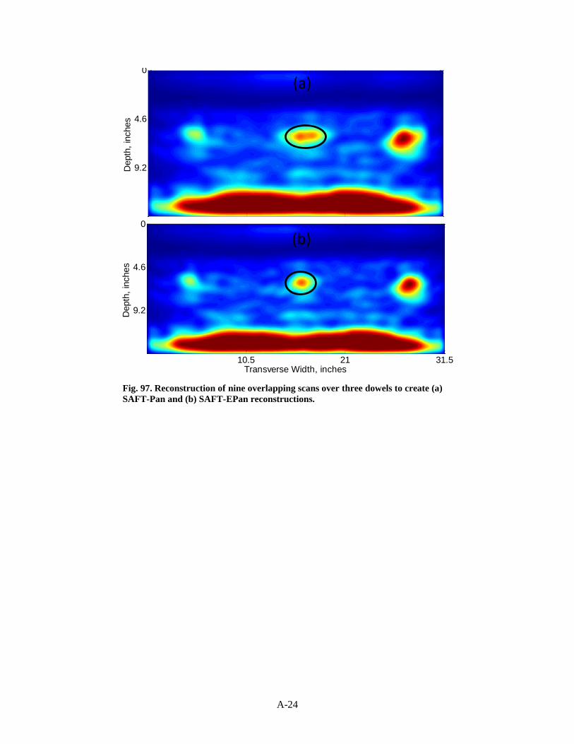
A-24
Fig. 97. Reconstruction of nine overlapping scans over three dowels to create (a)
SAFT-Pan and (b) SAFT-EPan reconstructions.
pos9pan
Transverse Width, inches
Depth
, in
ches
10.5 21 31.5
0
4.6
9.2
pos9pan
Transverse Width, inches
Depth
, in
ches
9.2 18.5 27.7
0
4.6
9.2
(b)
(a)

APPENDIX B. INTERPRETING ANTARES DATA FILES


B-3
APPENDIX B. INTERPRETING ANTARES DATA FILES
ANTARES Data Files (*.ANTDAT) are an ASCII text file type designed as a universal data file for data
produced by the native ANTARES NDE instruments. The files are tab-delimited and may be opened in
almost any data manipulation program including MATLAB and Microsoft Excel.
An *.ANTDAT file opened in Microsoft Excel will take on the following appearance
The header file indicates the program version, instrument, and time of file creation (start of ANTARES
scan). The grid settings table includes the origin information, line orientation, point and line spacings and
counts that will allow the user to recreate the grid if desired.
ANTARES grids begin at the given origin expressed in millimeters X and Y. The first point of the first
line is the origin itself. The first line will be oriented in either the X or Y direction as given, and will
consist of the number of points given by point count at a distance between points in millimeters given by
point spacing. The next line will be the number given by line spacing millimeters apart from the previous
until the total number of lines given by line count is achieved.
ANTARES SVW Data File
Program Version 1.0b
Instrument: Ultrasound (GI EyeCON)
Date/Time of creation: 6/10/2013 11:26
Grid Settings
Origin X 160
Origin Y 200
Line Orientation Y
Point Spacing 25
Line Spacing 25
Point Count 50
Line Count 77
Instrument Data
Time S-Coord X S-Coord Y I-Coord X I-Coord Y A-Scan
6/10/2013 11:26 160 200 268 249 1507328
6/10/2013 11:26 160 225 268 274 2097152
6/10/2013 11:26 160 250 268 299 1703936
B-4
The instrument data table consists of a number of rows equal to the total number of points taken during
the ANTARES scan. Each point is marked with a timestamp, X and Y coordinates of the scanner in
millimeters given by the “S-Coord” columns, and X and Y coordinates of the instrument as determined
from the mounted instrument head’s offset from the scanner coordinate system given by the “I-Coord”
columns. Finally, the A-Scan column indicates the data returned from the instrument itself. For single
point instruments such as the covermeter or laser profilometer, the A-Scan for each data point will be a
single cell under the A-Scan column. For the shear wave ultrasound instrument, the A-Scan is 2048
integer data points pertaining to a waveform and correspondingly occupy a range of 2048 cells populated
horizontally from the A-Scan column. For parallel instruments such as the GPR system, the A-Scan
column is blank as the data is stored locally on the instrument
Instrument A-Scan Data Type
Covermeter Cover in mm, 0 digits of precision
Laser Profilometer Distance in mm, 1 digit of precision
Ultrasound 2048 point 32 bit integer waveform
SCS Binary image string
GPR/Parallel Instrument Blank
Since each data point is furnished with its own coordinate, the data can be plotted directly from the
instrument data table in any suitable 2D intensity plot or 3D scatter plot where applicable.
Ultrasound waveform data is indexed in microseconds (μs), meaning each element in the 2048 element
array corresponds to intensity registered at a 1 μs delay from the previous element. It is advisable to store
Ultrasound waveform data as a 3D matrix using the grid settings to scale the axes on a 2D intensity plot
and index the third matrix dimension to produce a “fly-through” C-scan image similar to that produced by
the ANTARES Processing Software. Using this methodology, other dimensions of the 3D matrix can be
indexed to produce tomographic views of any desired orientation.