Evaluation of the Flow Quality in the MTL Wind-Tunnel Bj ...oso/papers/MTL_techrep.pdf · Evaluation of the Flow Quality in the MTL Wind-Tunnel by Bj orn Lindgren & Arne V. Johansson

Evaluation of the Flow Quality

in the MTL Wind-Tunnel

by

Bjorn Lindgren & Arne V. Johansson

Department of Mechanics

October 2002Technical Reports from

Royal Institute of TechnologyDepartment of Mechanics

SE-100 44 Stockholm, Sweden

Typsatt i AMS-LATEX med Osos rapport-stil.

c© Bjorn Lindgren & Arne V. Johansson 2002

Universitetsservice US AB, Stockholm 2002

ii

Contents

1. Introduction 1

2. Experimental setup 7

3. Results 12

4. Concluding remarks 29

5. Acknowledgment 30

References 30

Appendix 33

iii

iv

Evaluation of the flow quality in the MTL

wind-tunnel

By Bjorn Lindgren and Arne V. Johansson

Dept. of Mechanics, KTH, SE-100 44 Stockholm, Sweden

Technical report. TRITA-MEK 2002:13

The flow characteristics of the MTL wind-tunnel at the Department of Mechan-ics, KTH, have been evaluated 10 years after its completion. The wind-tunnelis of closed circuit type with a 7 m long test section that has a cross section areaof 1.2× 0.8 m2. The contraction ratio is 9 and the maximum speed is approx-imately 70 m/s. The experiments performed included measurements of totalpressure variation, temperature variation, flow angle variation and turbulenceintensity variation. The measurements were carried out in the test section overa cross flow measurement area of 0.9× 0.5 m2 located 0.4 m downstream theinlet. The temperature variation in time was also measured at the center of themeasurement area. The experiments were performed at three different wind-tunnel speeds, 10, 25 and 40 m/s. The present results confirm that the highflow quality of the MTL wind-tunnel. The flow quality measurements carriedout soon after the completion of the tunnel are here repeated and extended.For instance, at 25 m/s the streamwise turbulence intensity is less than 0.025%and both the cross flow turbulence intensities are less than 0.035% at the samespeed. The total pressure variation is less than ±0.06% and the temperaturevariation is less than ±0.05 ◦C.

1. Introduction

The Minimum Turbulence Level or Marten Theodore Landahl (MTL), wind-tunnel, named after its late initiator, was designed in the mid 80s to suitexperiments in basic transition and turbulence research. The wind-tunnel thatwas completed in 1991 has now been in operation for 10 years and it was decidedto re-confirm the early flow quality measurements and to extend them with theaid of the accurate and automated traversing equipment now in use. The Frenchcompany Sessia was contracted for the wind-tunnel construction, although theresponsibility for the aerodynamic design remained with the Department ofMechanics. The primary aim of the early tunnel calibration study was toperform experiments that could confirm that the design requirements in thecontract were fulfilled. The main results were reported in Johansson (1992).

1

2 B. Lindgren and A. V. Johansson

12

2

3

3 3

3

2

2

4

5

67

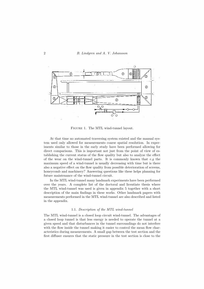
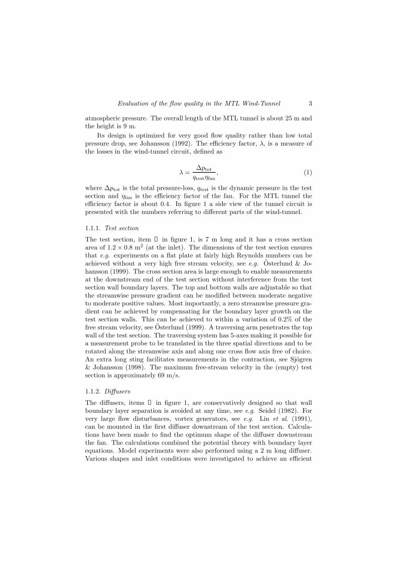
Figure 1. The MTL wind-tunnel layout.

At that time no automated traversing system existed and the manual sys-tem used only allowed for measurements coarse spatial resolution. In exper-iments similar to those in the early study have been performed allowing fordirect comparisons. This is important not just from the point of view of es-tablishing the current status of the flow quality but also to analyze the effectof the wear on the wind-tunnel parts. It is commonly known that e.g themaximum speed of a wind-tunnel is usually decreasing with time but is therealso a negative effect on the flow quality from possible deterioration of screens,honeycomb and machinery? Answering questions like these helps planning forfuture maintenance of the wind-tunnel circuit.

In the MTL wind-tunnel many landmark experiments have been performedover the years. A complete list of the doctoral and licentiate thesis wherethe MTL wind-tunnel was used is given in appendix 5 together with a shortdescription of the main findings in these works. Other landmark papers withmeasurements performed in the MTL wind-tunnel are also described and listedin the appendix.

1.1. Description of the MTL wind-tunnel

The MTL wind-tunnel is a closed loop circuit wind-tunnel. The advantages ofa closed loop tunnel is that less energy is needed to operate the tunnel at agiven speed and that disturbances in the tunnel surroundings do not interferewith the flow inside the tunnel making it easier to control the mean flow char-acteristics during measurements. A small gap between the test section and thefirst diffuser ensures that the static pressure in the test section is close to the

Evaluation of the flow quality in the MTL Wind-Tunnel 3

atmospheric pressure. The overall length of the MTL tunnel is about 25 m andthe height is 9 m.

Its design is optimized for very good flow quality rather than low totalpressure drop, see Johansson (1992). The efficiency factor, λ, is a measure ofthe losses in the wind-tunnel circuit, defined as

λ =∆ptot

qtestηfan

, (1)

where ∆ptot is the total pressure-loss, qtest is the dynamic pressure in the testsection and ηfan is the efficiency factor of the fan. For the MTL tunnel theefficiency factor is about 0.4. In figure 1 a side view of the tunnel circuit ispresented with the numbers referring to different parts of the wind-tunnel.

1.1.1. Test section

The test section, item ➀ in figure 1, is 7 m long and it has a cross sectionarea of 1.2× 0.8 m2 (at the inlet). The dimensions of the test section ensuresthat e.g. experiments on a flat plate at fairly high Reynolds numbers can beachieved without a very high free stream velocity, see e.g. Osterlund & Jo-hansson (1999). The cross section area is large enough to enable measurementsat the downstream end of the test section without interference from the testsection wall boundary layers. The top and bottom walls are adjustable so thatthe streamwise pressure gradient can be modified between moderate negativeto moderate positive values. Most importantly, a zero streamwise pressure gra-dient can be achieved by compensating for the boundary layer growth on thetest section walls. This can be achieved to within a variation of 0.2% of thefree stream velocity, see Osterlund (1999). A traversing arm penetrates the topwall of the test section. The traversing system has 5-axes making it possible fora measurement probe to be translated in the three spatial directions and to berotated along the streamwise axis and along one cross flow axis free of choice.An extra long sting facilitates measurements in the contraction, see Sjogren& Johansson (1998). The maximum free-stream velocity in the (empty) testsection is approximately 69 m/s.

1.1.2. Diffusers

The diffusers, items ➁ in figure 1, are conservatively designed so that wallboundary layer separation is avoided at any time, see e.g. Seidel (1982). Forvery large flow disturbances, vortex generators, see e.g. Lin et al. (1991),can be mounted in the first diffuser downstream of the test section. Calcula-tions have been made to find the optimum shape of the diffuser downstreamthe fan. The calculations combined the potential theory with boundary layerequations. Model experiments were also performed using a 2 m long diffuser.Various shapes and inlet conditions were investigated to achieve an efficient


diffuser without wall boundary layer separation. The conservative design ofthe diffusers leads to a longer wind-tunnel return circuit and is one contribut-ing factor to the relatively large total pressure-loss in this wind-tunnel circuitcompared to wind-tunnels used for commercial testing.

1.1.3. Corners

One wind tunnel part that could cause flow disturbances, and especially noiseis the corner, item ➂ in figure 1. The corner, which turns the flow 90◦, areequipped with a cascade of airfoils, here called guide-vanes. If the guide-vanesare not properly designed they could be exposed to large boundary layer sepa-rations leading to poor flow uniformity, large turbulence levels as well as hightotal pressure-loss. In the design of the MTL tunnel, special care was givento this detail with experiments and calculations performed by Sahlin & Jo-hansson (1991). In addition to the published results for profiles with turbulentboundary layers, a very efficient guide-vane with laminar boundary layers and atwo-dimensional total guide-vane pressure-loss coefficient as low as 0.036, mea-sured at the first corner downstream the test section, was designed for use inthe MTL-tunnel. Despite the very low pressure-loss the guide-vanes allows formoderate (±2◦) changes in angle of attack without separating. It is importantto design a guide-vane that will perform well under adverse flow conditionsespecially in the first corner where measurement equipment may disturb theflow substantially.

1.1.4. Driving unit

Item ➃ in figure 1 is the fan and motor. The fan used in the MTL tunnel isof axial type with 12 blades and the motor mounted directly onto the fan axis.The motor is of DC current type and it is enclosed in a cylinder with the samediameter as the fan hub for reasons of improved aerodynamics. It is cooledseparately by a fan outside the tunnel circuit and cooling air is supplied to theenclosed cylinder through elliptical pipes. This means that the heat generatedby losses in the motor does not need to be removed by the wind-tunnel heatexchanger. The power of the motor is 85 kW and the speed of the fan iscontrolled by a thyristor control unit.

In-front of and behind the fan there are silencers with central bodies tominimize noise disturbances from the fan. The upstream central body has thediameter of the fan hub and an ellipsoidal shaped nose cone. The central bodyof the downstream silencer is shaped as a cone with the base diameter equal-ing the upstream central body diameter. The upstream silencer also convertsthe tunnel circuit cross section from square to circular and the downstream si-lencer converts the cross section from circular to octagonal shape, which is theshape of the following diffuser, see figure 1. The walls of the silencers and theircentral bodies are made of perforated plates with a thick sound absorbing ma-terial (long fibered glass-wool covered by a woven glass-fiber material) for good


efficiency. The wind-tunnel parts located between the first and forth cornershave sound insulated walls, resulting in a very quiet wind-tunnel. Measure-ment of the noise level inside the test section was performed and are reportedin Johansson (1992).

1.1.5. Heat exchanger

The tunnel circuit heat exchanger, item ➄ in figure 1, is located at the lowerpart of the wind-tunnel just in-front of the third corner counting from the testsection in the downstream direction. This positioning of the heat exchanger isconservative in some sense of ensuring that the temperature variation in thetest section cross section is small. A small drawback of this positioning is thatthe cross section area is slightly higher here than in the stagnation chamber,see 1.1.6, leading to a small increase in local pressure drop.

The tubes of the heat exchanger are of elliptical cross section shape whichdecreases the local pressure drop slightly compared to standard circular pipes.Cooling flanges are mounted onto the pipes to increase the cooling area of theheat exchanger. Extra turbulence generators can also be added to the coolingflanges to enhance the heat transfer, but such items are not used here becauseof the very high pressure drop and the increase of the turbulence level causedby these turbulence generators.

The water flowing through the heat exchanger has a high and constantflow rate. It is cooled through an additional heat exchanger by water from anexternal, in-house, cooling system. A valve regulates the flow rate in the exter-nal system thereby controlling the temperature of the water passing throughthe wind-tunnel heat exchanger. This valve is regulated by a commercial PIDregulator.

The temperature in the wind-tunnel test section is measured by a PT-100sensor and is used as input into the PID regulator. The set, (chosen), wind-tunnel temperature is entered manually from the regulator front panel.

1.1.6. Stagnation chamber

The stagnation chamber, or settling chamber as it is often called, item ➅ infigure 1, has the largest cross section area, and thereby also the lowest flowvelocity, in the wind tunnel circuit. This is where items used for flow qualityimprovements are located such as screens and honeycomb. Sometimes the heatexchanger is also located here, see e.g. Seidel (1982), to minimize the localpressure-drop. This positioning was here rejected because of the ambition toachieve a high degree of temperature uniformity in the test section.

The MTL stagnation chamber consists of three different parts, the honey-comb, the screens and the relaxation duct, in that order of location relative tothe flow direction.


The purpose of the honeycomb is to break up large eddies into smaller onesand, more importantly, to rectify the flow coming from the fourth corner. Ascreen also rectifies the flow to some extent but the honeycomb is more efficientin this respect and it has a lower cost in pressure drop. The ratio between thelength, (in the streamwise direction), and the cell diameter of the honeycombis the most important parameter influencing the degree of flow rectification,see e.g. Lumley (1964); Loehrke & Nagib (1976); Scheiman & Brooks (1981).The honeycomb is 100 mm long and the cell diameter is about 10 mm in theMTL tunnel.

The screens on the other hand are more efficient than the honeycomb inreducing the turbulence by breaking down larger eddies into smaller ones with asize of the mesh width, see e.g. Laws & Livesey (1978) and Groth & Johansson(1988). The screens are also very effective in reducing mean flow variationsover the cross section area. This ability is related to the solidity, i.e. the ratioof blockage generated by the screen wire front area, and the pressure dropcoefficient of the screens, see Taylor & Batchelor (1949). It has been found thata combination of screens with decreasing mesh sizes in the downstream directionis very efficient in reducing mean flow variations, see e.g. Groth & Johansson(1988). The distance between the screens has to be more than about 30 meshsizes to let the screen wire induced turbulence die out sufficiently before it hitsthe next screen. The porosity of the screens must also be larger than about55% to avoid a phenomenon called jet collapse, see Baines & Peterson (1951).Jet collapse leads to a strong mean flow variation and must be avoided. In theMTL tunnel there are 5 screens with decreasing mesh size in the streamwisedirection between 3.1 mm and 0.75 mm. These values were chosen carefullyafter a study made by Groth & Johansson (1988) for maximum screen efficiency.

The effect of turbulence reduction of the screens is much larger in thestreamwise component than in the cross stream components of the flow. Thisis especially true for under-critical screens where up to 90% of the reductionis in the streamwise component, see Groth & Johansson (1988); Tan-Atichatet al. (1982). This means that the flow is very non-isotropic just downstreamof the screens making it important to allow the flow to relax towards a stateof isotropy before it enters the contraction where it again will be subjectedto high strains. This is achieved at the downstream end of the non-divergingstagnation chamber. The length of this section is 750 mm in the MTL tunnel,which is a long enough distance for the flow to reach an approximately isotropicstate.

1.1.7. Contraction

The final part in the wind-tunnel return circuit is the contraction, item ➆ infigure 1. It transform the wind-tunnel cross section area back to that of the testsection. The contraction also reduces the relative mean flow velocity variationand turbulence intensity. These reductions are much larger in the streamwise


direction than in the cross stream directions. They are also highly dependent onthe contraction ratio with increased reduction for increasing contraction ratio,see e.g. Johansson & Alfredsson (1988). The contraction ratio in the MTLtunnel is 9, i.e. the area ratio between the stagnation chamber and test sectioncross section areas. This value is rather high compared to most other wind-tunnels but there are occasional examples of even higher contraction ratios.The drawback of a high contraction ratio is the relative increase in tunnelreturn circuit length, highly non-isotropic flow in the test section inlet and anincreased risk for separating boundary layers on the contraction walls.

The shape of the contraction has to be designed very carefully to avoid wallboundary layer separation. A contraction can be divided into one upstreamconcave part and one downstream convex part. Separation can occur in boththese parts. A boundary layer separation is induced by a positive pressuregradient along the contraction wall and is caused by the curvature of the wall.It is present even though the mean flow in general is accelerating due to thedecrease in cross section area. Positive pressure gradients are found both in theconcave part close to the inflection point, where the shape of the walls becomeconvex, and at the downstream end of the convex part. A separation occurringin the concave part is very difficult to eliminate once the contraction is builtwhich means that it has to be avoided already at the design stage. A separationbubble in the convex part, however, can be eliminated by tripping the laminarboundary layer achieving transition to a turbulent boundary layer that is moreresistant to separation. This kind of boundary layer tripping is implementedin the MTL tunnel using V-shaped dymo-tape as roughness elements.

The shape of the contraction used in the MTL wind-tunnel was optimizedusing flow calculations. These calculations were based on a combination ofpotential theory and boundary layer equations. They were performed using acode that was provided by Downie et al. (1984). The aim was to minimize thecontraction length keeping a wall pressure gradient distribution without riskfor wall boundary layer separation. For further information on optimization ofthree dimensional wind-tunnel contractions see e.g. Borger (1976); Mikhail &Rainbird (1978).

The final shape chosen for the MTL-tunnel can be expressed as a combina-tion of sinus-hyperbolic functions where the concave part covers the first 70%of the contraction length and the convex part the remaining 30%.

2. Experimental setup

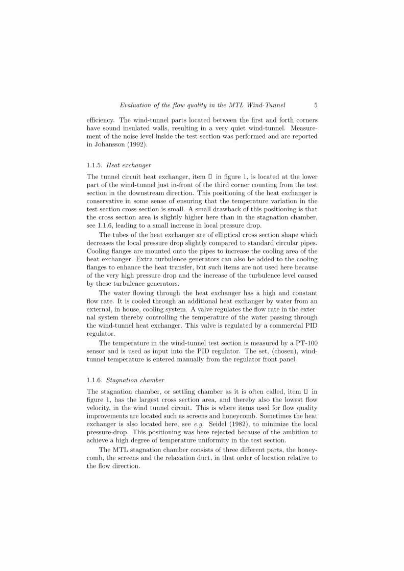
The present measurements were performed in a cross section of the test sectionat a position 400 mm downstream the test section entry. The area covered bythe measurement probes was 900 × 500 mm2 and located around the center,see figure 2. This area is here referred to as the measurement region. The arearatio between the measurement region and the test section is 0.47, thus almosthalf the total area is covered in the experiments. The reason for excluding the


Figure 2. The cross section of the test section. The hatchedarea is the area covered in the measurements.

150 mm wide rim closest to the walls is that the flow is here disturbed by thetunnel circuit walls and it is usually not included when figures of wind-tunnelflow qualities are compared. The velocity variation is stronger in the rim thanin the core region (measurement region). Therefore most experiments occurringin the MTL tunnel are performed in the core region. Also by excluding the rimthe calibration range of the probes can be minimized increasing the resolutionof the measurements in the core region. The measurements were performed atthree different test section free stream velocities covering a large part of thewind-tunnel velocity range. The three velocities are 10 m/s, 25 m/s, and 40m/s. These velocities were chosen because they are representative for manyof the experiments performed so far in the MTL tunnel. 10 m/s is a typicalvelocity for experiments on transition phenomena, 25 m/s is a typical velocityfor medium Reynolds number experiments and 40 m/s is a typical velocityfor higher Reynolds number experiments. The fan blade angles are not easilychanged and they are positioned for maximum performance at around 25 m/s.Therefore we expect the results of these measurements to be most favourableat 25 m/s free-stream velocity.

The traversing system used is a 5-axes system, see section 1.1.4. Thissystem can traverse a probe in the streamwise and cross stream directions. Itcan rotate the probe around its own axis and it can also change the angle ofattack. The last feature makes it possible to calibrate a cross wire probe ora flow angle probe without removing them from the test section, making thecalibration more accurate. The traversing system and the wind-tunnel velocityare controlled from a computer.


2.1. Measurement instrumentation

For the hot-wire measurements we used a two-channel anemometer, (AN-1003),from AA Labs (Israel). For further amplification of the hot-wire signal a stereoamplifier, (AX-490), from Yamaha was used. This amplifier was also used tofilter the signal, removing contributions from noise at very high frequencies.The signal was then sampled into a computer by a 12 bit AD board.

The measurement of the dynamic pressure was achieved through a differ-ential pressure transducer, (FCO510) from Furness Control, (Great Britain).The absolute accuracy of the pressure transducer is 0.25% of full scale, (±2000Pa). The sampled data are transfered to the measurement computer throughthe serial bus.

The temperatures were measured using Pt-100 sensors. The absolute ac-curacy of these sensors is in the order of 0.056 ◦C per ◦C. A 6 digit accuratemultimeter (HP-34401A) from Hewlett Packard with a built in 4-wire compen-sation resistance meter was used to measure the probe resistance. The 4-wirecompensation eliminates any contribution from the inherent resistance in theconnecting cables. The measured data was then transferred to the measurementcomputer through GPIB communication and then converted into temperaturesusing the following equation

Rt = R0

(

1 + AT + BT 2)

, (2)

where Rt is the probe resistance, R0 is the resistance at 0◦C, T is the temper-ature and A and B are constants.

2.2. Probe calibrations

The probes used were single- and cross- hot-wire probes and a flow angle probe.Calibrations of the hot-wire probes were performed immediately before everynew measurement. The flow angle probe was calibrated using several runs toverify the calibration accuracy.

2.2.1. Single-wire probe calibration

The exclusion of the near wall region allows the velocity range over which thecalibration is made to be very small. This means that the calibration can bemade with high accurately. The error in streamwise velocity for the single-wirecalibrations was less than ±0.05%. The single wire was calibrated in the freestream using King’s law

U0 =

(

E2 −A

B

)1

n

(3)


9.2 9.4 9.6 9.8 10 10.2 10.4 10.6 10.82.125

2.13

2.135

2.14

2.145

2.15

2.155

2.16

2.165

2.17

U0 (m/s)

E (V )

Figure 3. A typical calibration of a single-wire. The circlesare measured points and the solid line is the King’s law derivedby a least square fit to the measured points.

where U0 is the free-stream velocity, A, B and n are constants to be determinedand E is the voltage output from the anemometer. The mean velocity, U0, wasdetermined through the relationship

ptot − p =1

2ρU2

0 (4)

using a Prandtl tube to measure the dynamic pressure. The density and viscos-ity of the air could be determined accurately by measuring the static pressureand the temperature. In equation 4, ptot is the total pressure, p is the staticpressure and ρ is the air density. A typical single-wire calibration curve is seenin figure 3.

2.2.2. Cross-wire probe calibration

Calibrating the cross-wire probe includes variations both in the velocity andprobe angle of attack. A surface is then fitted to the measured data pointsusing a fifth order polynomial. The use of a polynomial that lacks any relevantphysical information makes it extra important not to allow any data pointsoutside the calibration range during measurements. This may lead to stronglyerroneous results.

The streamwise and cross stream velocities were determined by the equa-tions


U = U0 cosα, (5)

V = U0 sin α, (6)

where U and V are the streamwise and cross stream velocity components re-spectively and α is the probe angle of attack. Two help variables, x and yrepresenting the streamwise and the cross stream velocity components, are cal-culated from the wire voltages E1 and E2 as follows

x = E1 + E2, (7)

y = E1 −E2, (8)

These variables are then used to construct two two-dimensional fifth orderpolynomials, here denoted by M and N , for the two variables, U and tan α.By solving the following equations in a least square sense

MA = U, (9)

NB = tan α, (10)

the coefficients in the vectors A and B can be determined. These coefficients arethen stored and used later in the experiments to determine the instantaneousvelocities, u and v.

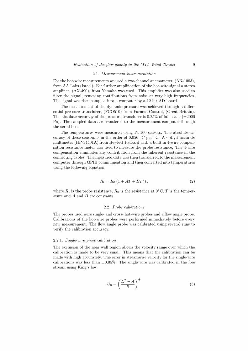
In figure 4 the results from a typical cross-wire calibration is shown. Thearea inside the solid lines is the calibration area where all measurement pointsmust lie. The error of the cross-wire calibration was less than ±0.05% for thestreamwise, U , component and the cross stream components V and W .

2.2.3. Flow angle probe calibration

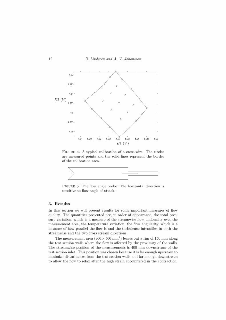
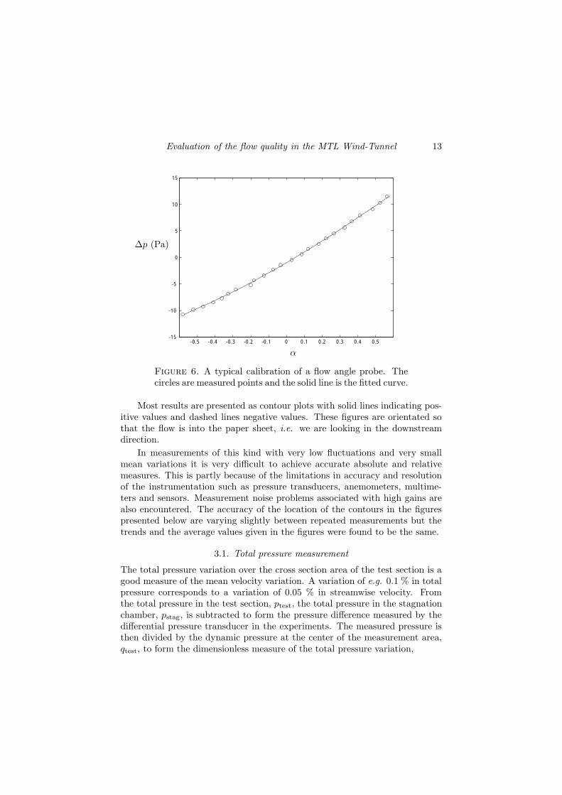
The flow angle probe was calibrated by altering the probe angle of attack inthe center of the measurement area. The shape of the probe makes it verysensitive to flow angle variations. There are two pressure holes, one on eachside of the probe close the bottom of the V-shaped cut, see figure 5. When thestagnation point at the bottom of the V cut moves towards one side a pressuredifference can be measured between the holes. The inclined edges of the V cutaccentuates this pressure difference. The pressure difference is measured fordifferent angles of attack and a least square fit of a third order polynomial isthen made to the measured data points. In figure 6 a typical calibration of aflow angle probe is shown. The error in the flow angle calibrations is less than±0.02◦.


4.61 4.615 4.62 4.625 4.63 4.635 4.64 4.645 4.65

4.79

4.795

4.8

4.805

4.81

4.815

4.82

E1 (V )

E2 (V )

Figure 4. A typical calibration of a cross-wire. The circlesare measured points and the solid lines represent the borderof the calibration area.

Figure 5. The flow angle probe. The horizontal direction issensitive to flow angle of attack.

3. Results

In this section we will present results for some important measures of flowquality. The quantities presented are, in order of appearance, the total pres-sure variation, which is a measure of the streamwise flow uniformity over themeasurement area, the temperature variation, the flow angularity, which is ameasure of how parallel the flow is and the turbulence intensities in both thestreamwise and the two cross stream directions.

The measurement area (900× 500 mm2) leaves out a rim of 150 mm alongthe test section walls where the flow is affected by the proximity of the walls.The streamwise position of the measurements is 400 mm downstream of thetest section inlet. This position was chosen because it is far enough upstream tominimize disturbances from the test section walls and far enough downstreamto allow the flow to relax after the high strain encountered in the contraction.


-0.5 -0.4 -0.3 -0.2 -0.1 0 0.1 0.2 0.3 0.4 0.5-15

-10

-5

0

5

10

15

α

∆p (Pa)

Figure 6. A typical calibration of a flow angle probe. Thecircles are measured points and the solid line is the fitted curve.

Most results are presented as contour plots with solid lines indicating pos-itive values and dashed lines negative values. These figures are orientated sothat the flow is into the paper sheet, i.e. we are looking in the downstreamdirection.

In measurements of this kind with very low fluctuations and very smallmean variations it is very difficult to achieve accurate absolute and relativemeasures. This is partly because of the limitations in accuracy and resolutionof the instrumentation such as pressure transducers, anemometers, multime-ters and sensors. Measurement noise problems associated with high gains arealso encountered. The accuracy of the location of the contours in the figurespresented below are varying slightly between repeated measurements but thetrends and the average values given in the figures were found to be the same.

3.1. Total pressure measurement

The total pressure variation over the cross section area of the test section is agood measure of the mean velocity variation. A variation of e.g. 0.1 % in totalpressure corresponds to a variation of 0.05 % in streamwise velocity. Fromthe total pressure in the test section, ptest, the total pressure in the stagnationchamber, pstag, is subtracted to form the pressure difference measured by thedifferential pressure transducer in the experiments. The measured pressure isthen divided by the dynamic pressure at the center of the measurement area,qtest, to form the dimensionless measure of the total pressure variation,


∆ptest(y, z)

qtest

=ptest(y, z)− pstag

qtest

(11)

where y and z are the vertical and horizontal directions.

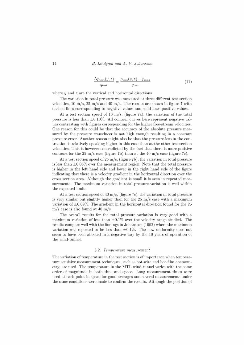
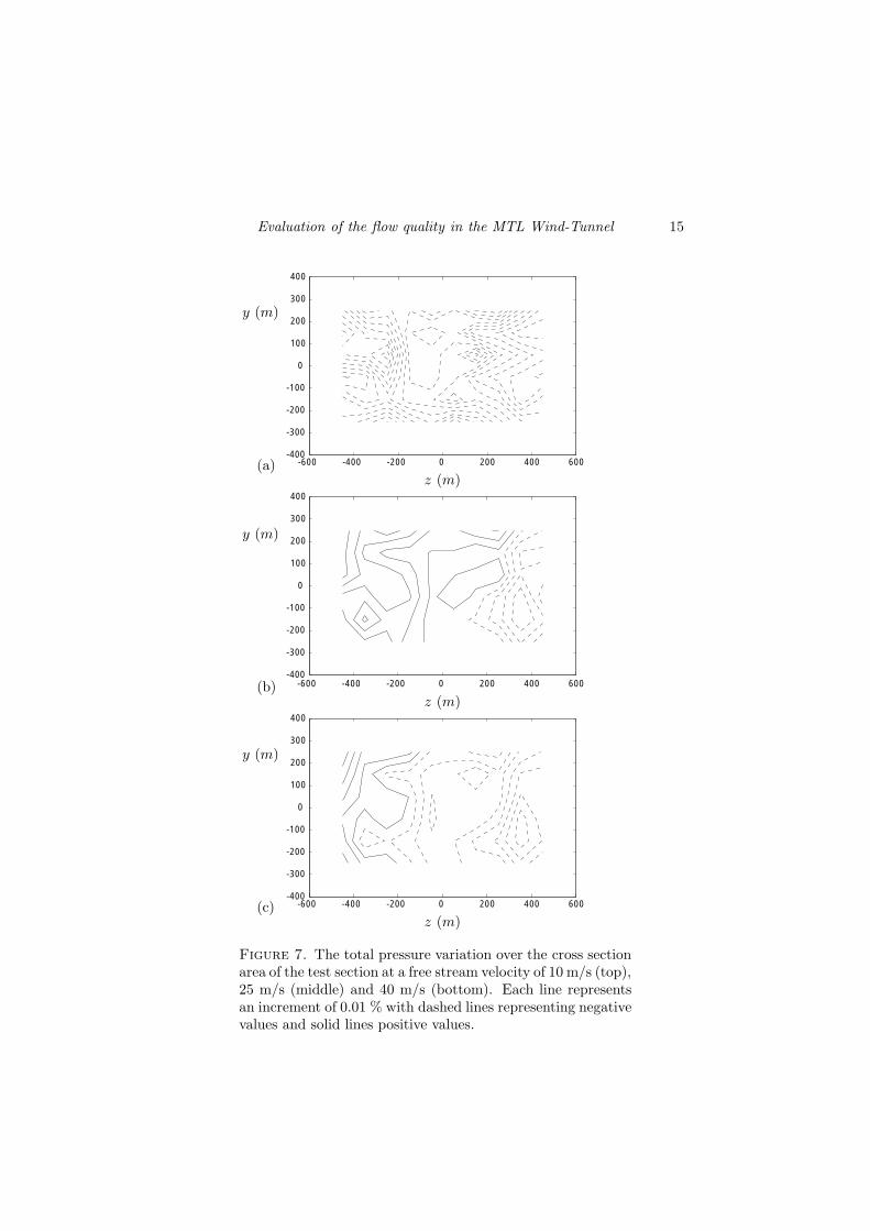
The variation in total pressure was measured at three different test sectionvelocities, 10 m/s, 25 m/s and 40 m/s. The results are shown in figure 7 withdashed lines corresponding to negative values and solid lines positive values.

At a test section speed of 10 m/s, (figure 7a), the variation of the totalpressure is less than ±0.10%. All contour curves here represent negative val-ues contrasting with figures corresponding for the higher free-stream velocities.One reason for this could be that the accuracy of the absolute pressure mea-sured by the pressure transducer is not high enough resulting in a constantpressure error. Another reason might also be that the pressure-loss in the con-traction is relatively speaking higher in this case than at the other test sectionvelocities. This is however contradicted by the fact that there is more positivecontours for the 25 m/s case (figure 7b) than at the 40 m/s case (figure 7c).

At a test section speed of 25 m/s, (figure 7b), the variation in total pressureis less than ±0.06% over the measurement region. Note that the total pressureis higher in the left hand side and lower in the right hand side of the figureindicating that there is a velocity gradient in the horizontal direction over thecross section area. Although the gradient is small it is seen in repeated mea-surements. The maximum variation in total pressure variation is well withinthe expected limits.

At a test section speed of 40 m/s, (figure 7c), the variation in total pressureis very similar but slightly higher than for the 25 m/s case with a maximumvariation of ±0.09%. The gradient in the horizontal direction found for the 25m/s case is also found at 40 m/s.

The overall results for the total pressure variation is very good with amaximum variation of less than ±0.1% over the velocity range studied. Theresults compare well with the findings in Johansson (1992) where the maximumvariation was reported to be less than ±0.1%. The flow uniformity does notseem to have been affected in a negative way by the 10 years of operation ofthe wind-tunnel.

3.2. Temperature measurement

The variation of temperature in the test section is of importance when tempera-ture sensitive measurement techniques, such as hot-wire and hot-film anemom-etry, are used. The temperature in the MTL wind-tunnel varies with the sameorder of magnitude in both time and space. Long measurement times wereused at each point in space for good averages and several measurements underthe same conditions were made to confirm the results. Although the position of


-600 -400 -200 0 200 400 600-400

-300

-200

-100

0

100

200

300

400

z (m)

y (m)

(a)

-600 -400 -200 0 200 400 600-400

-300

-200

-100

0

100

200

300

400

z (m)

y (m)

(b)

-600 -400 -200 0 200 400 600-400

-300

-200

-100

0

100

200

300

400

z (m)

y (m)

(c)

Figure 7. The total pressure variation over the cross sectionarea of the test section at a free stream velocity of 10 m/s (top),25 m/s (middle) and 40 m/s (bottom). Each line representsan increment of 0.01 % with dashed lines representing negativevalues and solid lines positive values.


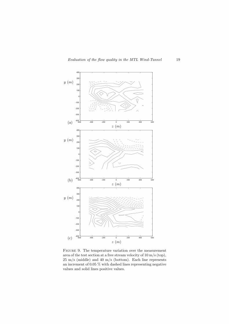
each curve in the contour plots in figure 9 varies slightly between the measure-ments the trends are always similar confirming repeatability. The temperaturecontours presented in figure 9 are calculated as the temperature deviation fromthe mid-range value normalized by the mean temperature (in ◦C), i.e.

∆T =T (y, z)− 1

2(Tmax(y, z) + Tmin(y, z))

T (y, z), (12)

where T is the temperature and y and z is the vertical and horizontal coor-dinates. The mid-range value is subtracted to give a clearer picture of thetemperature variation in the figure. The mean temperature in the measure-ments is about 20 ◦C.

The temperature variation over the measurement area in the test sectionwas measured at 10 m/s, 25 m/s and 40 m/s. The flow direction in the contourplots in figure 9 is into the paper sheet.

At 10 m/s the variation in temperature was less than ±0.2 % or ±0.04 ◦C,see figure 9a. This is a very small difference with the maximum temperaturepeak at about z = −250 mm and y = 50. This peak is also found at the othertwo tunnel speeds at a similar position. As was the case for the total pressuremeasurements the variation of the temperature over the cross section area atthis low velocity differs from the higher velocity cases. The trend in figure 9was confirmed by repeated measurements.

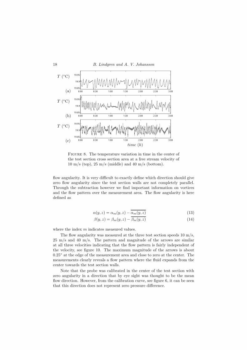
The variation in time is for the same test section velocity ±0.04 ◦C, seefigure 8a. This variation is of the same magnitude as the variation over thecross section area. The variation in time has a typical period of 300 s some-times interrupted by longer periods of more constant temperature. A hot-wiresampling time seldom exceeds 30 s which is one tenth of a period. A measure-ment can therefore occur at any time in the period. A hot-wire usually has atemperature of almost two hundred degrees making the errors small even be-tween samples taken at times coinciding with the high and low extreme pointsin the temperature oscillation.

At a test section speed of 25 m/s the temperature variation in space overthe measurement area was ±0.25 %, or ±0.05 ◦C see figure 9b. Here we find thepeak also present in the 10 m/s case at z = −350 mm and y = 50. Furthermore,it can be seen that the upper right corner is cooler than the lower left corner.A possible reason could be that the cooling water enters in the top right cornerand at the middle right side and that it exits at the lower right corner and themiddle right side.

The variation in time over a period of 3 hours was ±0.05 ◦C, see figure 8b,which is slightly higher than at the test section velocity of 10 m/s. The highertemperature at the beginning in figure 8b is ignored because it is remains fromthe settling time of the cooling system. The period of the fluctuation is about170 s which is almost half the period found at 10 m/s.


At the highest test section speed of 40 m/s the variation in space increasedfurther to a value of ±0.35 %, see figure 9c, or ±0.07 ◦C. The pattern ofvariation is very similar to the one found at 25 m/s and the peak at z = −350mm and y = 50 is still present.

The variation in time was about ±0.05 ◦C which is slightly higher thanfor the 25 m/s case, see figure 8c. The fluctuation period is here also 170 s.Overall the similarity between the 25 m/s and the 40 m/s cases are strong. Onedifference however is the increasing amplitude in the short time fluctuationsseen as a thickening of the line with increasing speed in figure 8. This is causedby the slow response time of the cooling system and it is the result of too longpiping between the heat exchangers and the constant flow rate of the coolingwater.

Comparing with the first study by Johansson (1992), that found a temper-ature variation of ±0.2 ◦C, the variation has improved mainly due to a bettersystem regulator. It is important to notice that the regulator, in this case, wasnot calibrated for each speed separately. This means that it probably is possi-ble to get a slightly steadier temperature in time than what is presented here.However, the process of finding the best calibration constants for the regulatoris rather time consuming. Therefore we did not do it here making our resultsa better representation for the temperature variations found in a typical MTLwind-tunnel experiment.

The settling time for the temperature, i.e. the time it takes to reach thedesired temperature in the test section with minimum fluctuations in time froma new start of the wind-tunnel is fairly long. E.g. at a test section velocity of25 m/s it takes approximately 30 minutes to stabilize the temperature. Thereason for these long settling times is the simple type of regulator used at themoment in the tunnel, (PID) and the long piping between the regulator valveand the heat exchanger. There have been a discussion of improving this systemin the future. A software based regulator with increased input information andimproved piping is used in a newly built wind-tunnel at the department, seeLindgren & Johansson (2002), and it has the potential to shorten the settlingtime and decrease the temperature variation from the values found here in theMTL wind-tunnel.

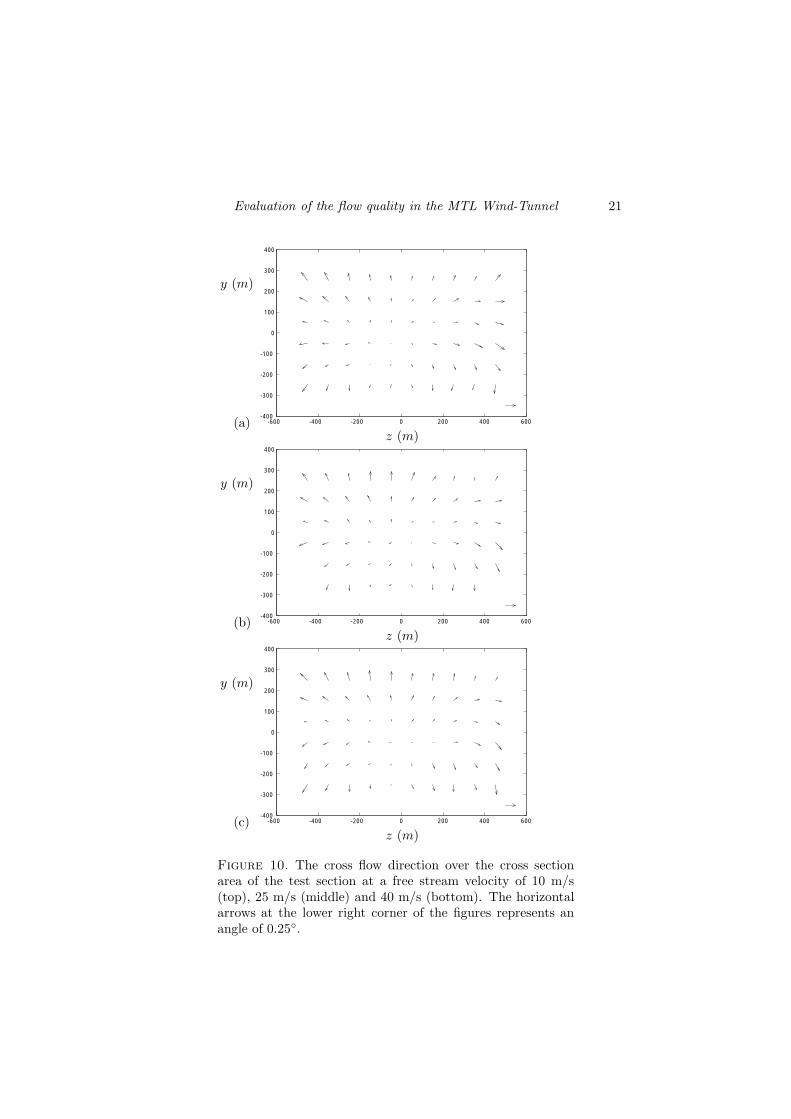
3.3. Flow angularity measurement

The flow angularity is a measure of the straightness of the flow i.e. the ratiobetween the two cross flow velocities and the streamwise velocity. The flowangle is calculated by measuring the pressure difference of two symmetricallyplaced holes on a special probe, see section 2.2.3. By rotating the probe 90◦

both cross stream components, α in the vertical direction and β in the hori-zontal direction, could be measured at the same position. The mean flow anglewas then subtracted from the measured values giving a relative measure of the


0:00 0:30 1:00 1:30 2:00 2:30 3:0019.85

19.9

19.95

0:00 0:30 1:00 1:30 2:00 2:30 3:0019.85

19.9

19.95

0:00 0:30 1:00 1:30 2:00 2:30 3:0019.85

19.9

19.95

time (h)

T (◦C)

(c)

T (◦C)

(b)

T (◦C)

(a)

Figure 8. The temperature variation in time in the center ofthe test section cross section area at a free stream velocity of10 m/s (top), 25 m/s (middle) and 40 m/s (bottom).

flow angularity. It is very difficult to exactly define which direction should givezero flow angularity since the test section walls are not completely parallel.Through the subtraction however we find important information on vorticesand the flow pattern over the measurement area. The flow angularity is heredefined as

α(y, z) = αm(y, z)− αm(y, z) (13)

β(y, z) = βm(y, z)− βm(y, z) (14)

where the index m indicates measured values.

The flow angularity was measured at the three test section speeds 10 m/s,25 m/s and 40 m/s. The pattern and magnitude of the arrows are similarat all three velocities indicating that the flow pattern is fairly independent ofthe velocity, see figure 10. The maximum magnitude of the arrows is about0.25◦ at the edge of the measurement area and close to zero at the center. Themeasurements clearly reveals a flow pattern where the fluid expands from thecenter towards the test section walls.

Note that the probe was calibrated in the center of the test section withzero angularity in a direction that by eye sight was thought to be the meanflow direction. However, from the calibration curve, see figure 6, it can be seenthat this direction does not represent zero pressure difference.


-600 -400 -200 0 200 400 600-400

-300

-200

-100

0

100

200

300

400

z (m)

y (m)

(a)

-600 -400 -200 0 200 400 600-400

-300

-200

-100

0

100

200

300

400

z (m)

y (m)

(b)

-600 -400 -200 0 200 400 600-400

-300

-200

-100

0

100

200

300

400

z (m)

y (m)

(c)

Figure 9. The temperature variation over the measurementarea of the test section at a free stream velocity of 10 m/s (top),25 m/s (middle) and 40 m/s (bottom). Each line representsan increment of 0.05 % with dashed lines representing negativevalues and solid lines positive values.


There are several possible reasons for this result. First there is an actualexpansion of the width of the test section, equal to 5 mm in 500 mm lengthor 0.06◦, at the streamwise position where the measurements were performed.However this is partly compensated for by the boundary layer growth whichis between 1.4 mm and 1.8 mm on each wall in the velocity range used here.There is also a slight variation in the height of the test section since the upperand lower walls are adjustable to compensate for wall boundary layer growthmaking it difficult to position them absolutely parallel. The slit in the roof,allowing the traversing sword to enter the test section, is not sealed allowingair to exit the test section due to the positive pressure encountered over theslit.

Johansson (1992) encountered flow angularities well below 0.1◦. This valueis much lower than the ones found in this study. The main reason for the largeincrease in flow angularity is probably that the slit in the Johansson (1992)study was completely sealed. During our measurements we opted for an openslit since this is the case for most experiments taking place in the MTL wind-tunnel. The rather large expansion of the width of the test section, 5 mm fromthe inlet to the measurement position, has not been reported earlier and it willalso contribute to an outwards directed flow. This expansion could be causedby swelling of the plywood test section walls as wood is a material that easilychanges shape and size with e.g. moisture and temperature.

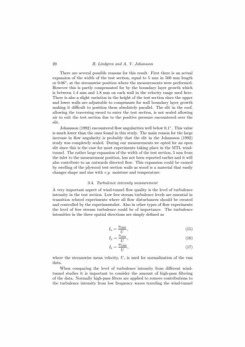
3.4. Turbulence intensity measurement

A very important aspect of wind-tunnel flow quality is the level of turbulenceintensity in the test section. Low free stream turbulence levels are essential intransition related experiments where all flow disturbances should be createdand controlled by the experimentalist. Also in other types of flow experimentsthe level of free stream turbulence could be of importance. The turbulenceintensities in the three spatial directions are simply defined as

Ix =urms

U, (15)

Iy =vrms

U, (16)

Iz =wrms

U, (17)

where the streamwise mean velocity, U , is used for normalization of the rmsdata.

When comparing the level of turbulence intensity from different wind-tunnel studies it is important to consider the amount of high-pass filteringof the data. Normally high-pass filters are applied to remove contributions tothe turbulence intensity from low frequency waves traveling the wind-tunnel


-600 -400 -200 0 200 400 600-400

-300

-200

-100

0

100

200

300

400

z (m)

y (m)

(a)

-600 -400 -200 0 200 400 600-400

-300

-200

-100

0

100

200

300

400

z (m)

y (m)

(b)

-600 -400 -200 0 200 400 600-400

-300

-200

-100

0

100

200

300

400

z (m)

y (m)

(c)

Figure 10. The cross flow direction over the cross sectionarea of the test section at a free stream velocity of 10 m/s(top), 25 m/s (middle) and 40 m/s (bottom). The horizontalarrows at the lower right corner of the figures represents anangle of 0.25◦.


circuit. The cut-off frequency is always chosen in a somewhat arbitrary man-ner. In this case we wanted all disturbances with wave lengths fitting in the testsection cross section area to be conserved. Allowing for some margin we chosethe wave length as the sum of the two test section side lengths, i.e. the cut-offwave length was chosen to be 2.0 m. A large part of the fluctuating energy isfound at low frequencies which means that the filter can easily reduce the rmsvalue by 50%. In this section the results will be provided for both unfilteredand high-pass filtered data. to simplify comparisons with results from otherwind-tunnels and to visualize the impact of the filtering.

The cut-off frequency, fc, is calculated from the free stream mean velocity,U and the cut-off wave length, λc as follows

fc =U

λc. (18)

The rms values are calculated by summation of the square of the absolutevalue of the Fourier coefficients from the time signal. The high-pass filtering isapplied by summing only over the frequencies above the cut-off frequency. Therms values for the three velocity components thus read

urms =

2

N/2∑

k=Nc

|Xi|2

1

2

, (19)

vrms =

2

N/2∑

k=Nc

|Yi|2

1

2

, (20)

wrms =

2

N/2∑

k=Nc

|Zi|2

1

2

, (21)

where X , Y and Z are the Fourier coefficients corresponding to the velocitytime signals u(x, y; t)−U(x, y), v(x, y; t)−V (x, y) and w(x, y; t)−W (x, y). N isthe total number of samples and Nc is the summation index, k, correspondingto the frequency fc.

The turbulence intensities were measured at the three different wind-tunnelspeeds, 10 m/s, 25 m/s and 35 m/s. Note the change in velocity from 40 m/s to35 m/s for the highest test section speed case compared to the previous resultspresented in this section. The reason for this is the influence from vibrationsand acoustic noise from the probe holder devices at high speeds. The flowdisturbances are very small and have much of their energy at low frequencies,typical also of vibrating stings, making it increasingly important to avoid thesevibrations. The high-pass filtering could help removing vibrations. However,


there is no guarantee that these measurements are fully free from unwanteddisturbances.

In the earlier study by Johansson (1992), measurements up to 60 m/s wereobtained using another more rigid traversing arm. The increased flexibility andmaneuverability of the traversing arm has here been exchanged with a lowermaximum test section speed. The cut-off wave length in the Johansson (1992)study was 2.5 m which is slightly different from the one used in this study. Thiswill have some effect on the results in the streamwise direction and less in theother two directions.

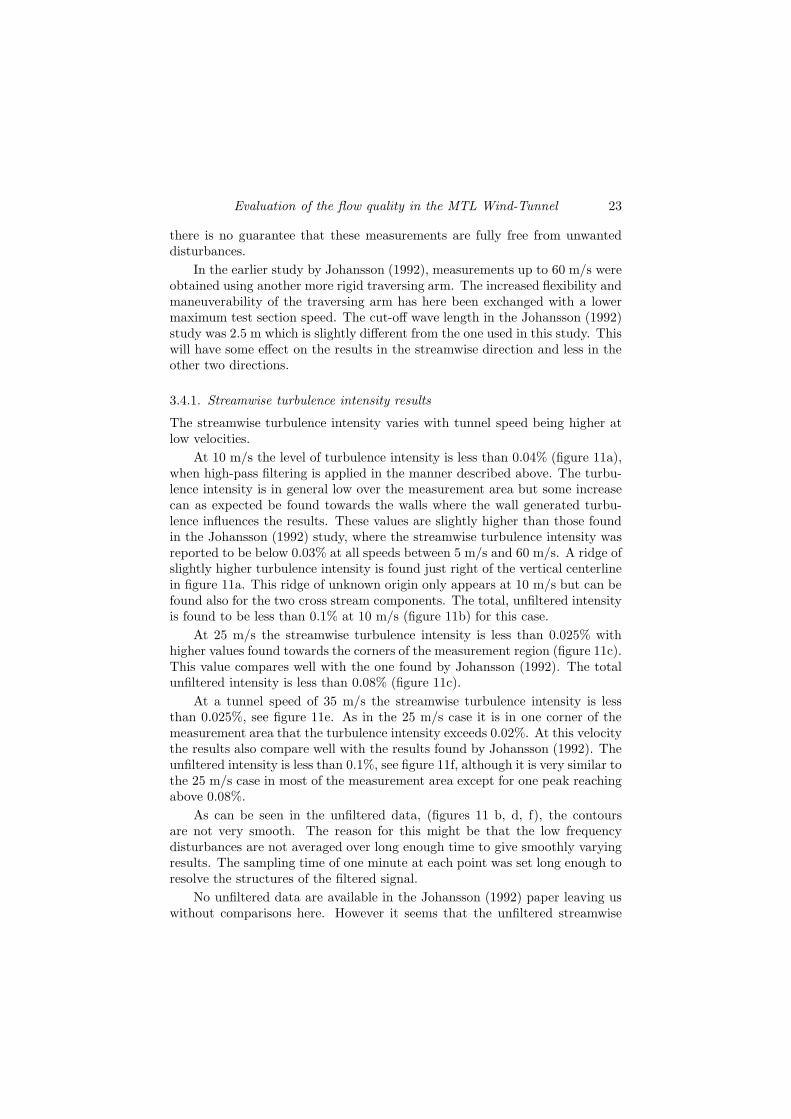
3.4.1. Streamwise turbulence intensity results

The streamwise turbulence intensity varies with tunnel speed being higher atlow velocities.

At 10 m/s the level of turbulence intensity is less than 0.04% (figure 11a),when high-pass filtering is applied in the manner described above. The turbu-lence intensity is in general low over the measurement area but some increasecan as expected be found towards the walls where the wall generated turbu-lence influences the results. These values are slightly higher than those foundin the Johansson (1992) study, where the streamwise turbulence intensity wasreported to be below 0.03% at all speeds between 5 m/s and 60 m/s. A ridge ofslightly higher turbulence intensity is found just right of the vertical centerlinein figure 11a. This ridge of unknown origin only appears at 10 m/s but can befound also for the two cross stream components. The total, unfiltered intensityis found to be less than 0.1% at 10 m/s (figure 11b) for this case.

At 25 m/s the streamwise turbulence intensity is less than 0.025% withhigher values found towards the corners of the measurement region (figure 11c).This value compares well with the one found by Johansson (1992). The totalunfiltered intensity is less than 0.08% (figure 11c).

At a tunnel speed of 35 m/s the streamwise turbulence intensity is lessthan 0.025%, see figure 11e. As in the 25 m/s case it is in one corner of themeasurement area that the turbulence intensity exceeds 0.02%. At this velocitythe results also compare well with the results found by Johansson (1992). Theunfiltered intensity is less than 0.1%, see figure 11f, although it is very similar tothe 25 m/s case in most of the measurement area except for one peak reachingabove 0.08%.

As can be seen in the unfiltered data, (figures 11 b, d, f), the contoursare not very smooth. The reason for this might be that the low frequencydisturbances are not averaged over long enough time to give smoothly varyingresults. The sampling time of one minute at each point was set long enough toresolve the structures of the filtered signal.

No unfiltered data are available in the Johansson (1992) paper leaving uswithout comparisons here. However it seems that the unfiltered streamwise


turbulence intensity has increased somewhat over the years. This can be theresult of dirt accumulation in honeycomb, screens and heat exchanger. Partlydue to the increase in the usage of smoke recently for LDV, PIV and visual-ization measurements and to changes in fan blade angles for high pressure-lossexperiments. After these measurements were completed it was found that therewas an error in the manufacturing of the fan bearings leading to their destruc-tion. The bearings have now been changed making the fan run more smoothly.A thorough cleaning of the tunnel and tuning of the fan blade angles wouldprobably improve the unfiltered turbulence intensity results.

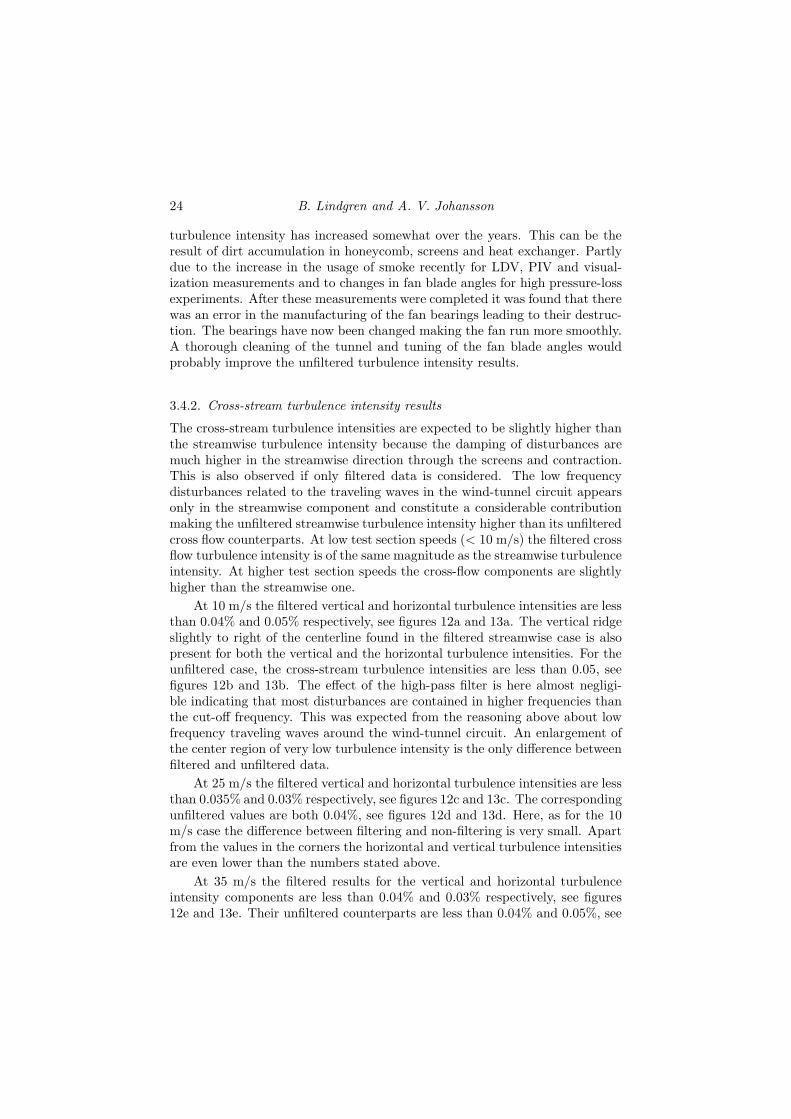
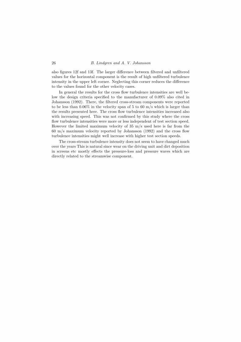
3.4.2. Cross-stream turbulence intensity results

The cross-stream turbulence intensities are expected to be slightly higher thanthe streamwise turbulence intensity because the damping of disturbances aremuch higher in the streamwise direction through the screens and contraction.This is also observed if only filtered data is considered. The low frequencydisturbances related to the traveling waves in the wind-tunnel circuit appearsonly in the streamwise component and constitute a considerable contributionmaking the unfiltered streamwise turbulence intensity higher than its unfilteredcross flow counterparts. At low test section speeds (< 10 m/s) the filtered crossflow turbulence intensity is of the same magnitude as the streamwise turbulenceintensity. At higher test section speeds the cross-flow components are slightlyhigher than the streamwise one.

At 10 m/s the filtered vertical and horizontal turbulence intensities are lessthan 0.04% and 0.05% respectively, see figures 12a and 13a. The vertical ridgeslightly to right of the centerline found in the filtered streamwise case is alsopresent for both the vertical and the horizontal turbulence intensities. For theunfiltered case, the cross-stream turbulence intensities are less than 0.05, seefigures 12b and 13b. The effect of the high-pass filter is here almost negligi-ble indicating that most disturbances are contained in higher frequencies thanthe cut-off frequency. This was expected from the reasoning above about lowfrequency traveling waves around the wind-tunnel circuit. An enlargement ofthe center region of very low turbulence intensity is the only difference betweenfiltered and unfiltered data.

At 25 m/s the filtered vertical and horizontal turbulence intensities are lessthan 0.035% and 0.03% respectively, see figures 12c and 13c. The correspondingunfiltered values are both 0.04%, see figures 12d and 13d. Here, as for the 10m/s case the difference between filtering and non-filtering is very small. Apartfrom the values in the corners the horizontal and vertical turbulence intensitiesare even lower than the numbers stated above.

At 35 m/s the filtered results for the vertical and horizontal turbulenceintensity components are less than 0.04% and 0.03% respectively, see figures12e and 13e. Their unfiltered counterparts are less than 0.04% and 0.05%, see


-400 -300 -200 -100 0 100 200 300 400

-200

-100

0

100

200

0.03

0.02

0.02 0.02

0.03

-400 -300 -200 -100 0 100 200 300 400

-200

-100

0

100

200

0.08

0.060.08 0.06 0.04

0.06

0.08

0.06

0.040.08

0.06

z (m)

y (m)

(a) z (m)

y (m)

(b)

-400 -300 -200 -100 0 100 200 300 400

-200

-100

0

100

2000.02

0.015

0.015

0.015

0.015

-400 -300 -200 -100 0 100 200 300 400

-200

-100

0

100

200

0.06

0.06

0.06

0.06

0.06 0.06

0.06 0.04

0.06

0.04

0.06

0.06

0.04

0.04

z (m)

y (m)

(c) z (m)

y (m)

(d)

-400 -300 -200 -100 0 100 200 300 400

-200

-100

0

100

200 0.02

0.015

0.015

0.02

-400 -300 -200 -100 0 100 200 300 400

-200

-100

0

100

200

0.06

0.02 0.04

0.06

0.04

0.04

0.04

0.04

0.06

0.04

0.06

0.08

0.04

z (m)

y (m)

(e) z (m)

y (m)

(f)

Figure 11. The streamwise turbulence intensity variation in% over the cross section area of the test section at a free streamvelocity of 10 m/s (top), 25 m/s (middle) and 35 m/s (bottom).The left column represents the high pass filtered data withU/fc = 2.0 m and the right column represents unfiltered data.


also figures 12f and 13f. The larger difference between filtered and unfilteredvalues for the horizontal component is the result of high unfiltered turbulenceintensity in the upper left corner. Neglecting this corner reduces the differenceto the values found for the other velocity cases.

In general the results for the cross flow turbulence intensities are well be-low the design criteria specified to the manufacturer of 0.09% also cited inJohansson (1992). There, the filtered cross-stream components were reportedto be less than 0.06% in the velocity span of 5 to 60 m/s which is larger thanthe results presented here. The cross flow turbulence intensities increased alsowith increasing speed. This was not confirmed by this study where the crossflow turbulence intensities were more or less independent of test section speed.However the limited maximum velocity of 35 m/s used here is far from the60 m/s maximum velocity reported by Johansson (1992) and the cross flowturbulence intensities might well increase with higher test section speeds.

The cross-stream turbulence intensity does not seem to have changed muchover the years This is natural since wear on the driving unit and dirt depositionin screens etc mostly effects the pressure-loss and pressure waves which aredirectly related to the streamwise component.


-400 -300 -200 -100 0 100 200 300 400

-200

-100

0

100

200

0.02

0.01

0.02

0.02

0.030.02

-400 -300 -200 -100 0 100 200 300 400

-200

-100

0

100

200

0.02

0.03 0.020.03

0.03

0.04

0.04

z (m)

y (m)

(a) z (m)

y (m)

(b)

-400 -300 -200 -100 0 100 200 300 400

-200

-100

0

100

2000.02

0.025

0.03 0.03

0.025

-400 -300 -200 -100 0 100 200 300 400

-200

-100

0

100

200 0.03

0.02

0.03

0.030.03

z (m)

y (m)

(c) z (m)

y (m)

(d)

-400 -300 -200 -100 0 100 200 300 400

-200

-100

0

100

2000.035

0.03

0.025

0.035

-400 -300 -200 -100 0 100 200 300 400

-200

-100

0

100

200

0.03

0.04 0.04

0.03

0.03

z (m)

y (m)

(e) z (m)

y (m)

(f)

Figure 12. The vertical cross stream turbulence intensityvariation over the cross section area of the test section at afree stream velocity of 10 m/s (top), 25 m/s (middle) and 35m/s (bottom). The left column represents the high pass fil-tered data with U/fc = 2.0 m and the right column representsunfiltered data.


-400 -300 -200 -100 0 100 200 300 400

-200

-100

0

100

200

0.01

0.01

0.02

0.02

0.02

0.02

0.03

0.04

-400 -300 -200 -100 0 100 200 300 400

-200

-100

0

100

200

0.02

0.03

0.02

0.030.04

0.03

0.04

z (m)

y (m)

(a) z (m)

y (m)

(b)

-400 -300 -200 -100 0 100 200 300 400

-200

-100

0

100

200 0.02

0.02

0.0150.020.025

-400 -300 -200 -100 0 100 200 300 400

-200

-100

0

100

200

0.02

0.02

0.03

0.03

0.03

z (m)

y (m)

(c) z (m)

y (m)

(d)

-400 -300 -200 -100 0 100 200 300 400

-200

-100

0

100

2000.025

0.025

0.02

0.02

0.02

0.02 0.02

0.02

0.02

0.02

0.025

0.025

0.025

0.02

-400 -300 -200 -100 0 100 200 300 400

-200

-100

0

100

200 0.030.03

0.04

0.03

z (m)

y (m)

(e) z (m)

y (m)

(f)

Figure 13. The horizontal cross stream turbulence intensityvariation over the cross section area of the test section at afree stream velocity of 10 m/s (top), 25 m/s (middle) and 35m/s (bottom). The left column represents the high pass fil-tered data with U/fc = 2.0 m and the right column representsunfiltered data.


4. Concluding remarks

The flow quality in the MTL wind-tunnel at the Department of Mechanics,KTH has been investigated. It was also studied in connection with the con-struction of the wind-tunnel. The results from these early measurements arereported in Johansson (1992). The reason for performing new measurementswere both to improve the documentation of the flow quality and to investigatehow the flow quality has changed after 10 years of extensive use of the facility.In the new experiments the same quantities as in the early experiment havebeen measured except for static pressure variations over the test section mea-surement area. It was measured in the early experiment but left out here dueto the high difficulty in achieving results not influenced by changes in dynamicpressure.

The total pressure variation over the test section cross section area is lessthan ±0.06% at a test section speed of 25 m/s and slightly larger at 10 m/s and40 m/s. These results are well in line with those found earlier by Johansson(1992) that reported a total pressure variation of less than ±0.1% over a testsection velocity range of 5 to 60 m/s. The variation in total pressure variationhas not been severely effected by time.

The temperature variation over the measurement area was found to beless than ±0.05 ◦C, (at 25 m/s), which is substantially smaller than the initialfindings by Johansson (1992) of ±0.2 ◦C, due to a better control of the coolingsystem.

The temporal variation of the temperature is less than ±0.04◦C at a testsection speed of 10 m/s and ±0.05◦C at test section speeds of 25 m/s and40 m/s. The temperature variation in time is thus similar to the variation inspace.

The flow angularity was measured over the measurement area using a spe-cial probe that is very sensitive to a change in position of the stagnation point.The results show a maximum deviation of 0.25◦ at the edges of the measure-ment area at all test section velocities. The flow is directed outwards towardsthe test section walls around the measurement area edge. The reason for thisoutwards directed flow is an increase in the cross section area of the test sectionin the vicinity of the downstream measurement position, partly compensatedfor by boundary layer growth, and the unsealed slit in the upper wall allowingair to flow out from the test section where the static pressure is slightly largerthan the atmospheric pressure outside. A comparison with the earlier measure-ments by Johansson (1992) shows that the flow angle variation observed in thepresent investigation is substantially larger, partly because of the introductionof the traversing system. The maximum flow angularity was in the early studybelow 0.1◦.

The turbulence intensity has been measured in the streamwise and thevertical and horizontal cross-stream directions. At a test section velocity of 25


m/s the streamwise turbulence intensity was found to be less than 0.025% andthe vertical and horizontal cross-stream turbulence intensity components wasless than 0.035% and 0.03% respectively. Here, the data was high-pass filteredremoving structures with wave lengths longer than 2.0 m. At the other speedsinvestigated (10 and 35 m/s) the intensities were found to be somewhat higher.

These results compares well with those found by Johansson (1992) and theyare within the original design criteria. The unfiltered streamwise turbulenceintensity is higher than what was expected but it can probably be loweredby adjusting the fan blade angles and cleaning the wind-tunnel screens, guidevanes and heat exchanger.

In general the MTL wind-tunnel still has an overall flow quality to welljustify the name, Minimum Turbulence Level. Some deterioration has beennoticed mainly in flow angularity and unfiltered turbulence levels. These prob-lems are though thought to be of such nature that a minor overhaul could wellbe enough to restore the initial performance. The general flow quality indi-cates a good potential for the MTL wind-tunnel to be a high-quality tool intransition and turbulence research also for the coming ten years. The increaseduse of optical measurement methods, such as LDV and PIV requiring seeding,implies an increased need for regular cleaning of the interior of the tunnel.

5. Acknowledgment

The authors would like to thank Valeria Duranona from the Technical Uni-versity of Uruguay, Montevideo, Uruguay, for assistance in some of the mea-surements. Further thanks goes to Ulf Landen for his aid in manufacturingthe measurement equipment. Henrik Alfredsson is greatfully acknowledged formany comments on the manuscript and for sharing the main responsibility ofthe planning and design of the MTL wind-tunnel with the second author. Fi-nally financial support from the Swedish Research Council for the first authoris greatfully acknowledged.

References

Baines, W. & Peterson, E. 1951 An investigation of flow through screens. Trans.

ASME 73, 467–480.

Boiko, A. V., Westin, K. J. A., Klingmann, B. G. B., Kozlov, V. V. &

Alfredsson, P. H. 1994 Experiments in a boundary layer subjected to free-stream turbulence. part 2. the role of TS-waves in the transition process. J. Fluid

Mech 281, 219–245.

Borger, G. G. 1976 The optimization of wind tunnel contractions for the subsonicrange. Tech. Rep. TTF 16899. NASA.


Downie, J. H., Jordinson, R. & Barnes, F. H. 1984 On the design of three-dimensional wind tunnel contractions. J. Royal Aeronautical Society pp. 287–295.

Elofsson, P. A. & Alfredsson, P. H. 1998 An experimental study of obliquetransition in plane poiseuille flow. J. Fluid Mech 358, 177–202.

Groth, J. & Johansson, A. V. 1988 Turbulence reduction by screens. J. Fluid

Mech 197, 139–155.

Haggmark, C. P., Bakchinov, A. A. & Alfredsson, P. H. 2000 Experiments ona two-dimensional laminar separation bubble. Phil. Trans. R. Soc. Lond. A 28.

Johansson, A. V. 1992 A low speed wind-tunnel with extreme flow quality-designand tests. Proc. the 18:th ICAS Congress pp. 1603–1611.

Johansson, A. V. & Alfredsson, P. H. 1988 Experimentella metoder i

stromningsmekaniken. Department of Mechanics, Royal Institute of Technology.

Laws, E. & Livesey, J. 1978 Flow through screens. Ann rev Fluid Mech. 10, 247–266.

Lin, J. C., Selby, G. V. & Howard, F. G. 1991 Exploratory study of vortex-generating devices for turbulent flow separation control. In 29th AIAA Aerospace

Sciences Meeting, Reno, Nevada. AIAA paper 91-0042.

Lindgren, B. & Johansson, A. V. 2002 Design and calibration of a low-speed wind-tunnel with expanding corners. TRITA-MEK 2002:14. Department of Mechanics,KTH.

Loehrke, R. I. & Nagib, H. M. 1976 Control of free-stream turbulence by meansof honeycombs: A balence between suppression and generation. J. Fluids Engi-

neering pp. 342–353.

Lumley, J. L. 1964 Passage of turbulent stream through honeycombs of large length-to-diameter ratio. Trans. ASME, J. Basic Engineering 86, 218–220.

Matsubara, M. & Alfredsson, P. H. 2001 Disturbance growth in boundary layerssubjected to free stream turbulence. J. Fluid Mech. 430, 149–168.

Mikhail, M. N. & Rainbird, W. J. 1978 Optimum design of wind tunnel contrac-tions, paper 78-819. In AIAA 10th Aerodynamic Testing Conference.

Osterlund, J. M. 1999 Experimental studies of zero pressure-gradient turbulentboundary-layer flow. PhD thesis, Department of Mechanics, Royal Institute ofTechnology, Stockholm.

Osterlund, J. M. & Johansson, A. V. 1999 Turbulent boundary layer experi-ments in the MTL wind-tunnel. TRITA-MEK 1999:16. Department of Mechan-ics, KTH.

Osterlund, J. M., Johansson, A. V., Nagib, H. M. & Hites, M. H. 2000 A noteon the overlap region in turbulent boundary layers. Phys. Fluids 12, 1–4.

Sahlin, A. & Johansson, A. V. 1991 Design of guide vanes for minimizing thepressure loss in sharp bends. Phys. Fluids A 3, 1934–1940.

Scheiman, J. & Brooks, J. D. 1981 Comparison of experimental and theoreticalturbulence reduction from screens, honeycomb and honeycomb-screen combina-tions. JAS 18, 638–643.

Seidel, M. 1982 Construction 1976-1980. design, manufacturing, calibration of the


German-Dutch wind tunnel (DNW). Tech. Rep.. Duits-Nederlandese Windtun-nel (DNW).

Sjogren, T. & Johansson, A. V. 1998 Measurement and modelling of homogeneousaxisymmetric turbulence. J. Fluid Mech 374, 59–90.

Tan-Atichat, J., Nagib, H. M. & Loehrke, R. I. 1982 Interaction of free-streamturbulence with screens and grids: a balance between tubulence scales. J. Fluid

Mech. 114, 501–528.

Taylor, G. & Batchelor, G. K. 1949 The effect of wire gauze on small disturbancesin a uniform stream. Quart. J. Mech. and App. Math. 2, part 1,1.

Westin, K. J. A., Boiko, A. V., Klingmann, B. G. B., Kozlov, V. V. &

Alfredsson, P. H. 1994 Experiments in a boundary layer subjected to free-stream turbulence. Part 1. Boundary layer structure and receptivity. J. Fluid

Mech 281, 193–218.

Wikstrom, P. M., Hallback, M. & Johansson, A. V. 1998 Measurements andheat-flux transport modelling in a heated cylinder wake. Int. J. Heat and Fluid

Flow 19, 556–562.


Appendix

Here follows a list of the Doctoral and Licentiate theses so far produced at theDepartment of Mechanics, KTH, where experiments performed in the MTLwind-tunnel are included. There is also a list of selected papers, not includedin a thesis, based on experiments in the MTL tunnel.

Doctoral theses in chronological order

1. JOHAN GROTH, On the modeling of homogeneous turbulence, 1991,ISRN KTH/MEK/TR–91/00–SE.Groth’s thesis includes work on screen turbulence which was used indetermining the size and number of screens to have in the MTL wind-tunnel. These results are also published in Groth & Johansson (1988).

2. TORBJORN SJOGREN, Development and calibration of turbulencemodels through experiment and computation, 1997,ISRN KTH/MEK/TR–97/05–SE.Torbjorn Sjogren performed the first experiment where the pressure-strain rate term in (statistically) axisymmetric turbulence was directlymeasured. These results are also presented in Sjogren & Johansson(1998).

3. JOHAN WESTIN, Laminar turbulent boundary layer transition influ-enced by free stream turbulence, 1997,ISRN KTH/MEK/TR–97/10–SE.Results concerning non-parallel effects on boundary-layer stability werefound and these results are reported in Westin et al. (1994) and Boikoet al. (1994).

4. PER ELOFSSON, Experiments on oblique transition in wall boundedshear flows, 1998, ISRN KTH/MEK/TR–98/05–SE.Per Elofsson made investigations of the role of oblique transition inPoiseuille and Blasius flows which are reported in Elofsson & Alfredsson(1998).

5. PETRA WIKSTROM, Measurements, direct numerical simulation andmodeling of passive scalar transport in turbulent flows, 1998,ISRN KTH/MEK/TR–98/11–SE.Experiments on passive scalars (temperature) in a cylinder wake wereperformed. Special care was taken to measure the Reynolds fluxes. Seealso Wikstrom et al. (1998).

6. JENS OSTERLUND, Experimental studies of zero pressure-gradientturbulent boundary layer flow, 1999, ISRN KTH/MEK/TR–99/16–SE.

Jens Osterlund established the log-law for z.p.g. turbulent boundarylayer flow and determined new values for the Karman and additive con-stants. These findings are reported in Osterlund et al. (2000).


7. CARL HAGGMARK, Investigations of disturbances developing in alaminar separation bubble flow, 2000,ISRN KTH/MEK/TR–00/03–SE.Investigations were made on highly instable high frequency two-dimensionalwaves in a laminar separation bubble, see Haggmark et al. (2000).

Licentiate theses in chronological order

1. KRISTIAN ANGELE, PIV measurements in a separating turbulentAPG boundary layer, 2000, ISRN KTH/MEK/TR–00/15–SE.This work focuses on scaling and structures of in a turbulent separationbubble.

2. JENS FRANSSON, Investigations of the asymptotic suction boundarylayer, 2001, ISRN KTH/MEK/TR–01/11–SE.This work is mainly focused on the study of the asymptotic suctionboundary layer.

Selected papers in chronological order

Other papers, not included in a thesis from the Department of Mechanics,involving measurements in the MTL wind-tunnel are listed below.

1. Sahlin & Johansson (1991)Alexander Sahlin was part of the MTL aerodynamic design team. Amongother things he developed the guide-vanes used in the present tunnel.He was also heavily involved in the calibration of the wind-tunnel.

2. Matsubara & Alfredsson (2001)Matsubara has made experiments on instabilities and their growth inlaminar boundary layers. Some of which are reported in the above citedpaper.

Ongoing theses/post doc work

There are still work in process in the MTL wind-tunnel that will be publishedin the future. In the list below, the people currently involved in measurementsin the MTL wind-tunnel, are listed in alphabetical order.

1. Kristian Angele, (Dr. thesis work)Title: Turbulent flow separation.

2. Jens H. M. Fransson, (Dr. thesis work)Title: Investigations of the asymptotic suction boundary layer.

3. Bjorn Lindgren, (Dr. thesis work)Title: Flow facility design and experimental studies of wall boundedturbulent shear-flows

4. Fredrik Lundell, (Dr. thesis work)Title: An experimental study of by-pass transition and its control.


5. Davide Medici, (Dr. thesis work)Title: Non-axisymmetric wakes and the possibility to optimize the poweroutput of wind-turbine farms.

6. Shuya Yoshioka, (Post. Doc. work)Title: Boundary layer suction for reduction of friction drag.

Documents

Evaluation of the Flow Quality in the MTL Wind-Tunnel Bj ...oso/papers/MTL_techrep.pdf · Evaluation of the Flow Quality in the MTL Wind-Tunnel by Bj orn Lindgren & Arne V. Johansson