Embed Size (px)
Citation preview
HAL Id: hal-01863448https://hal.archives-ouvertes.fr/hal-01863448
Preprint submitted on 28 Aug 2018
HAL is a multi-disciplinary open accessarchive for the deposit and dissemination of sci-entific research documents, whether they are pub-lished or not. The documents may come fromteaching and research institutions in France orabroad, or from public or private research centers.
L’archive ouverte pluridisciplinaire HAL, estdestinée au dépôt et à la diffusion de documentsscientifiques de niveau recherche, publiés ou non,émanant des établissements d’enseignement et derecherche français ou étrangers, des laboratoirespublics ou privés.
Evaluation of the Fair Credit Risk Premium inCommercial Lending
Sofiane Aboura, Emmanuel Lépinette
To cite this version:Sofiane Aboura, Emmanuel Lépinette. Evaluation of the Fair Credit Risk Premium in CommercialLending. 2018. hal-01863448
Evaluation of the Fair Credit RiskPremium in Commercial Lending
Sofiane Aboura,1 Emmanuel Lepinette2,3
1Universite de Paris XIII, Sorbonne Paris Cite, 93430 Villetaneuse, France.Email: [email protected]
2 Ceremade, PSL National Research, UMR CNRS 7534, Place du Marechal De LattreDe Tassigny, 75775 Paris cedex 16, France.
Email: [email protected]
3Gosaef, Faculte des Sciences de Tunis, 2092 Manar II-Tunis, Tunisia.
Abstract: We consider the problem of characterizing and computingthe fair credit risk premium that a firm should pay when borrowingmoney from a bank. Using a risk-neutral approach, we show that thereis a unique credit risk premium for a commercial loan depending on thefirm’s strategy such that the expected discounted value of the bank’spayoff coincides with the loan’s par value. We then propose a numericalprocedure to estimate the premium.
Keywords and phrases: Corporate Loans, Credit Risk, InvestmentDecisions, Portfolio Choice, Contingent Pricing2000 MSC: 60G44, G11-G13, G32-G33.
1
/ 2
1. Introduction
This paper discusses the pricing of corporate loans in the case where the riskpremium is explicitly related to the firm’s investment strategy.
A corporate loan is seen as a bilateral financial agreement issued, in theform of periodic payments, by a bank for its corporate non-financial firms.The main difference between loans and bonds is that banks are senior tobondholders in bankruptcy (Schwert, 2018). Loans are typically unsecured,which places the bank on equal level with unsecured bondholders, althoughit is unusual for a firm to default on an unsecured loan1. Of course, a firmcan also borrow money by issuing unsecured corporate bonds in the loanmarket. To that end, Santos (2011) finds that after the sub-prime crisis,banks increased the interest rates on their loans to bank-dependent borrow-ers by more than they did on their loans to borrowers that have access tothe bond market. This result is also confirmed by Schwert (2018) who showsthat firms are willing to pay a higher cost to borrow from a bank due tothe bank specialness. In clear, it seems there exists a preference for banksdespite a relatively higher cost. The overall cost for a loan can be seen as thebasis point spread over the money market rate (the main reference rate forcorporate loans is Libor) plus the annual fees over the life of the loan.
The pricing of loan contracts has attracted considerable research interest2.The pricing structure can depend on the type of loans (Credit Lines versusTerm Loans) as explained by Berg et al. (2017)3 as some loan contracts are setwith repayment on maturity (zero-coupon plan), while others are designed
1Schwert (2018) gives the example of the average recovery rate for loans that is 80%whereas it is 40% for bonds, which implies that loan credit spreads should be smallerthan bond credit spreads. From these aggregated statistics, he argues that the Duffie andSingleton (1999) model predicts that bond spreads should be approximately three timesas large as loan spreads. More precisely, when the firm is close to default, bond spreadsare significantly higher than loan spreads, but when it is far from default, the loan andbond spreads are similar.
2See Papin (2013)’s doctoral dissertation for an interesting discussion on that topic.3In term loans, firms receive generally the full loan amount upfront and repay the loan
at maturity, 5-8 years after loan origination, while other term loans are amortized untilmaturity. Credit lines are more frequent and more complex as they provide contingentliquidity, i.e. they do not draw down the committed loan amount, but keep the credit lineas an insurance. The pricing structure of credit lines is more complex as it consists ofvarious fees in addition to the loan spread.
/ 3
with amortization plans (periodical payments plan).
An important problem with loan pricing comes from the assessment ofthe default probability. Credit risk is generally calculated implicitly from theprice of loans, as it includes the investors expectation about future possiblelosses. But in practice, this information is provided by credit-rating agen-cies that compute long-term historical default rates for various horizons oftime. These corporate credit ratings reduce the gap in terms of informa-tion asymmetry between lenders and borrowers to find an equilibrium price(Blochlinger, 2018). The corresponding credit scoring is an important in-strument in setting an appropriate default premium when determining therate of interest charged to the borrower company with a past credit history.Hence, the loan spreads reflect the ex-ante credit risk as they are stronglycorrelated with probabilities of borrower default and capture the loan’s creditrisk smoothed through the cycle (Lee, Liu and Stebunovs, 2017). However,the credit rating does not incorporate the forward looking market consensusof the default risk and overall, it seems that past corporate bond spreadsappear to have poor predictive power over default rates (Giesecke, Longstaff,Schaefer, and Strebulaev, 2011).A related prominent problem with loan contracts is the determination of thefair risk premium that reflects the level of risk of the borrower’s project. Eachrisky loan carries a risk premium for which the current price is the expectedvalue of the pay-off discounted at the risk-free interest rate augmented bya risk premium. Loan risk premiums correspond to the loan rates less therisk-free rates and lower risk premiums arise when they carry lower losses dueto default. In case of high risk profile for the borrowing firm, the bank canlimit its exposure by requiring the riskier borrowers to select only short-termloans or imposing a collateral asset for hedging purpose. Interestingly, Allen,Scott and Vasso (2016) explain that in fact lenders offer a menu of contractterms such that applicants with higher-quality projects choose secured debtwith lower risk premiums, while applicants with lower-quality projects self-select into unsecured debt with higher risk premiums. The valuation problembecomes relying on the firm’s investment strategy given the relation betweenthe quality of a project and the associated risk premium.
To that end, the present paper considers credit risk from the perspective of abank willing to lend money according to the strategy of a non-financial firm.The very question is how large the minimum credit interest rate the bank re-

/ 4
quires should be for it to compensate for the risk not to be reimbursed giventhe firm’s strategy? This paper considers the realistic case where the bankhas to fix the fair risk premium depending on the firm’s strategy expressedin terms of quality of investment and level of consumption.
The article is organized as follows. Section 2 displays the literature review.Section 3 outlines the model. In Section 4, the main results are presentedwith their mathematical proofs. Section 5 concludes.
2. Review of literature
In financial theory, credit risk is defined as the case where the asset valueends up below the level of debts driving the firm to be insolvent. The fun-damental contribution of the Merton (1974)’s structural model is that firm’risky debt can be viewed as a pseudo-bond equal to a portfolio composedof a risk-free debt minus a short put option on the value of the firm’ assets.Structural models jointly capture the capital structure along with the evolu-tion of firm asset value (Lee, Liu and Stebunovs, 2017). The structural modelgives rational restrictions on the pricing of corporate debt and equity claimson a levered firm through classical option pricing theory (Black and Scholes,1973; Merton, 1973) and classical corporate finance theory (Modigliani andMiller, 1958). This derivatives-based approach gives rational for pricing loansunder a risk-neutral framework.
Important extensions of the Merton (1974)’s structural model has been doneso far (Geske, 1977; Ingersoll, 1977) and particularly for credit risk becauseMerton model credit spreads are too low regarding what market prices. Theliterature refers to this phenomenon as the ”credit spread puzzle” to explainwhy actual credit spreads are well above the theoretical spreads predicted bythe debt valuation models begining from the seminal Merton (1974) model.
There is an extensive theoretical literature examining this credit spreadpuzzle through the pricing of bonds in the presence of credit risk. Among themain pieces of work, study of the effects of safety covenants giving the bond-holders the right to bankrupt and restrictions on the financing of interestand dividend payments (Black and Cox, 1976); pricing of contingent claimson the term structure of interest rates (Ho and Lee, 1986; Heath, Jarrow,Morton, 1992); derivation of solution for risky debts for finite maturity and

/ 5
stochastic risk-free interest rate (Longstaff and Schwartz, 1992); connectionof debt value to firm risk, taxes, bankruptcy cost and bond covenants (Le-land, 1994); valuation of risky corporate debt that incorporates both defaultand interest rate risk (Longstaff and Schwartz, 1995); pricing of derivativessecurities involving credit risk (Jarrow and Turbull, 1995); optimal default(Leland and Toft, 1996); pricing of interest-rate swap yields with a standardterm structure model incorporating default risk (Duffie and Singleton, 1997);agency costs (Leland, 1998); asymmetric information and uncertainty (Duffieand Lando, 2001); relation between risk premium in corporate bond pricesand firms’ investment and financing policies (Kuehn and Schmid, 2014); com-plex debt structures with multiple bonds and various covenants (Liu, Dai andWang, 2016); idiosyncratic asset uncertainty measure as the residual volatil-ity from a market model on equity (Culp, Nozawa and Veronesi, 2018).
However, Collin-Dufresne, Goldstein, and Martin (2001) find that creditspreads are driven by factors difficult to explain by standard credit mod-els, which has been confirmed by Giesecke, Longstaff, Schaefer, and Strebu-laev (2011) who study corporate bond default rates using an extensive dataset (1866-2008). In fact, several assumptions behind these structural modelstend to deviate the results from real world observations (Liu, Dai and Wang,2016). For instance, the structural models tend to simplify the capital struc-ture to build mathematical models that are tractable but fail to capture thecomplexity of debt structure (Eom, Helwege and Huang, 2004). In addition,structural models have difficulty in simultaneously explaining both the de-fault probabilities and true credit spreads particularly for investment-gradebonds (Huang and Huang, 2012).
This paper adds to the broad literature on structural models of firm by de-riving the fair value of the credit risk premium as being explicitly related tothe firm’s strategy. The novelty is to define the firm’s strategy as a combi-nation of the investment strategy (portfolio of risky assets) along with thefinancial policy (deleveraging ratio) and the dividend policy (pay-out ratio).Whatsoever, this fair pricing relies on the ability of the bank to share thesame level of information with the borrowing non-financial firm.
/ 6
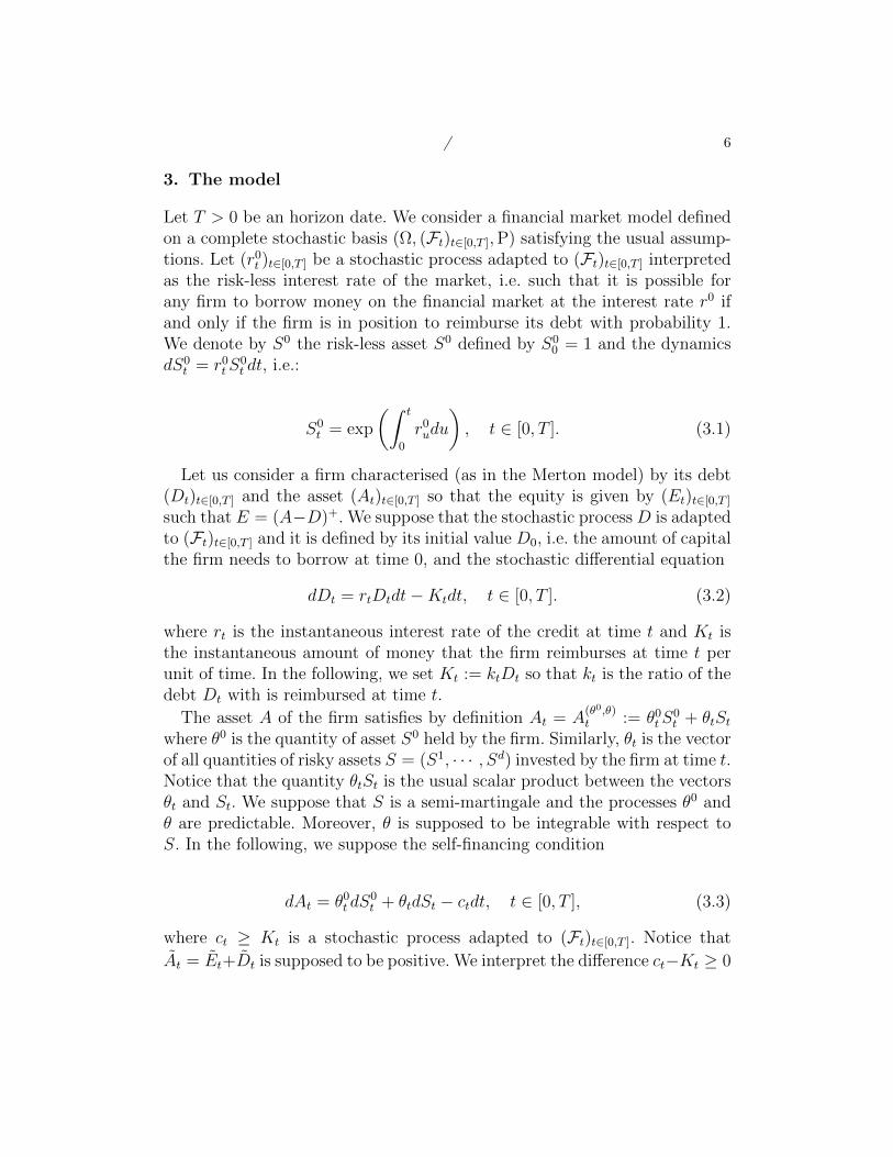
3. The model
Let T > 0 be an horizon date. We consider a financial market model definedon a complete stochastic basis (Ω, (Ft)t∈[0,T ],P) satisfying the usual assump-tions. Let (r0t )t∈[0,T ] be a stochastic process adapted to (Ft)t∈[0,T ] interpretedas the risk-less interest rate of the market, i.e. such that it is possible forany firm to borrow money on the financial market at the interest rate r0 ifand only if the firm is in position to reimburse its debt with probability 1.We denote by S0 the risk-less asset S0 defined by S0
0 = 1 and the dynamicsdS0
t = r0tS0t dt, i.e.:
S0t = exp
(∫ t
0
r0udu
), t ∈ [0, T ]. (3.1)
Let us consider a firm characterised (as in the Merton model) by its debt(Dt)t∈[0,T ] and the asset (At)t∈[0,T ] so that the equity is given by (Et)t∈[0,T ]such that E = (A−D)+. We suppose that the stochastic process D is adaptedto (Ft)t∈[0,T ] and it is defined by its initial value D0, i.e. the amount of capitalthe firm needs to borrow at time 0, and the stochastic differential equation
dDt = rtDtdt−Ktdt, t ∈ [0, T ]. (3.2)
where rt is the instantaneous interest rate of the credit at time t and Kt isthe instantaneous amount of money that the firm reimburses at time t perunit of time. In the following, we set Kt := ktDt so that kt is the ratio of thedebt Dt with is reimbursed at time t.
The asset A of the firm satisfies by definition At = A(θ0,θ)t := θ0tS
0t + θtSt
where θ0 is the quantity of asset S0 held by the firm. Similarly, θt is the vectorof all quantities of risky assets S = (S1, · · · , Sd) invested by the firm at time t.Notice that the quantity θtSt is the usual scalar product between the vectorsθt and St. We suppose that S is a semi-martingale and the processes θ0 andθ are predictable. Moreover, θ is supposed to be integrable with respect toS. In the following, we suppose the self-financing condition
dAt = θ0t dS0t + θtdSt − ctdt, t ∈ [0, T ], (3.3)
where ct ≥ Kt is a stochastic process adapted to (Ft)t∈[0,T ]. Notice that
At = Et+Dt is supposed to be positive. We interpret the difference ct−Kt ≥ 0
/ 7
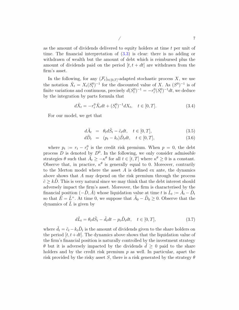
as the amount of dividends delivered to equity holders at time t per unit oftime. The financial interpretation of (3.3) is clear: there is no adding orwithdrawn of wealth but the amount of debt which is reimbursed plus theamount of dividends paid on the period [t, t + dt] are withdrawn from thefirm’s asset.
In the following, for any (Ft)t∈[0,T ]-adapted stochastic process X, we use
the notation Xt = Xt(S0t )−1 for the discounted value of X. As (S0)−1 is of
finite variations and continuous, precisely d(S0t )−1 = −r0t (S0
t )−1dt, we deduce
by the integration by parts formula that
dXt = −r0t Xtdt+ (S0t )−1dXt, t ∈ [0, T ]. (3.4)
For our model, we get that
dAt = θtdSt − ctdt, t ∈ [0, T ], (3.5)
dDt = (pt − kt)Dtdt, t ∈ [0, T ], (3.6)
where pt := rt − r0t is the credit risk premium. When p = 0, the debtprocess D is denoted by D0. In the following, we only consider admissiblestrategies θ such that At ≥ −κθ for all t ∈ [t, T ] where κθ ≥ 0 is a constant.Observe that, in practice, κθ is generally equal to 0. Moreover, contrarilyto the Merton model where the asset A is defined ex ante, the dynamicsabove shows that A may depend on the risk premium through the processc ≥ kD. This is very natural since we may think that the debt interest shouldadversely impact the firm’s asset. Moreover, the firm is characterised by thefinancial position (−D, A) whose liquidation value at time t is Lt := At− Dt
so that E = L+. At time 0, we suppose that A0 − D0 ≥ 0. Observe that thedynamics of L is given by
dLt = θtdSt − dtdt− ptDtdt, t ∈ [0, T ], (3.7)
where dt = ct−ktDt is the amount of dividends given to the share holders onthe period [t, t+dt]. The dynamics above shows that the liquidation value ofthe firm’s financial position is naturally controlled by the investment strategyθ but it is adversely impacted by the dividends d ≥ 0 paid to the shareholders and by the credit risk premium p as well. In particular, apart therisk provided by the risky asset S, there is a risk generated by the strategy θ
/ 8
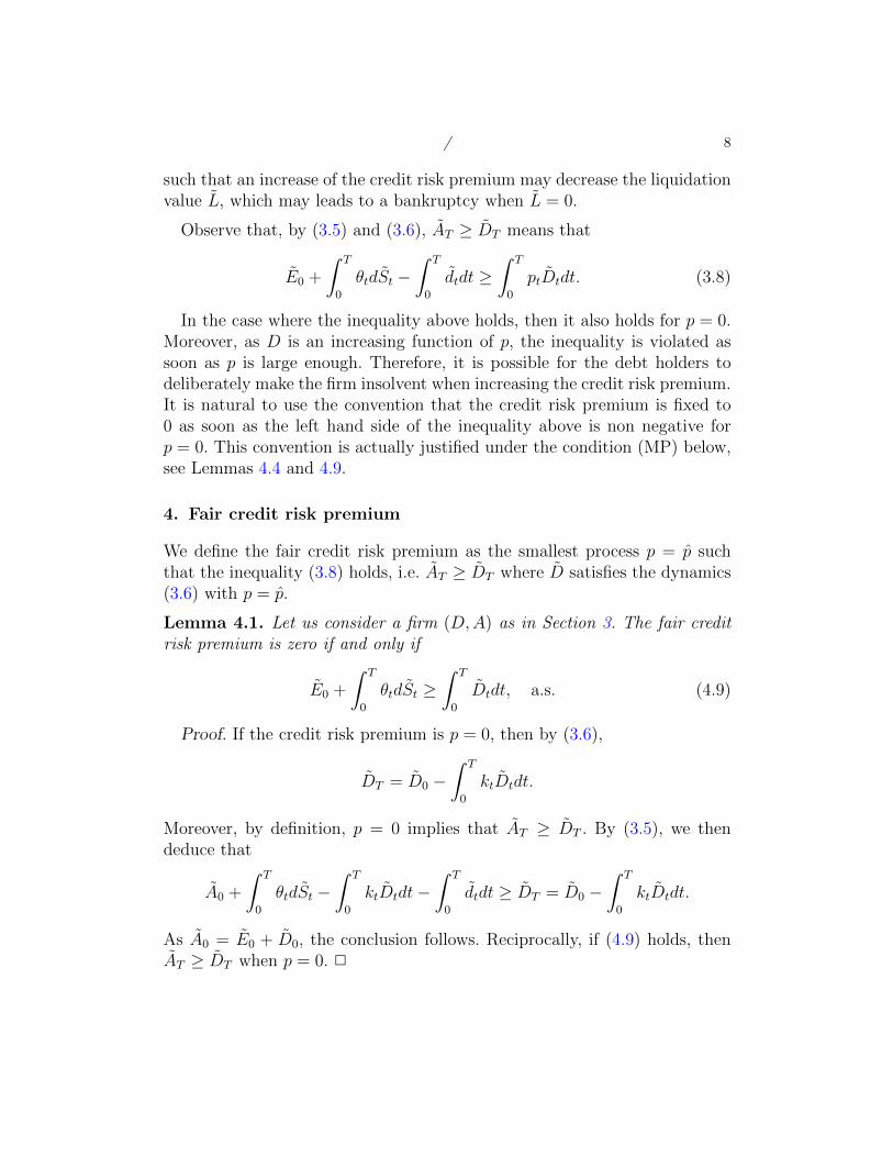
such that an increase of the credit risk premium may decrease the liquidationvalue L, which may leads to a bankruptcy when L = 0.
Observe that, by (3.5) and (3.6), AT ≥ DT means that
E0 +
∫ T
0
θtdSt −∫ T
0
dtdt ≥∫ T
0
ptDtdt. (3.8)
In the case where the inequality above holds, then it also holds for p = 0.Moreover, as D is an increasing function of p, the inequality is violated assoon as p is large enough. Therefore, it is possible for the debt holders todeliberately make the firm insolvent when increasing the credit risk premium.It is natural to use the convention that the credit risk premium is fixed to0 as soon as the left hand side of the inequality above is non negative forp = 0. This convention is actually justified under the condition (MP) below,see Lemmas 4.4 and 4.9.
4. Fair credit risk premium
We define the fair credit risk premium as the smallest process p = p suchthat the inequality (3.8) holds, i.e. AT ≥ DT where D satisfies the dynamics(3.6) with p = p.
Lemma 4.1. Let us consider a firm (D,A) as in Section 3. The fair creditrisk premium is zero if and only if
E0 +
∫ T
0
θtdSt ≥∫ T
0
Dtdt, a.s. (4.9)
Proof. If the credit risk premium is p = 0, then by (3.6),
DT = D0 −∫ T
0
ktDtdt.
Moreover, by definition, p = 0 implies that AT ≥ DT . By (3.5), we thendeduce that
A0 +
∫ T
0
θtdSt −∫ T
0
ktDtdt−∫ T
0
dtdt ≥ DT = D0 −∫ T
0
ktDtdt.
As A0 = E0 + D0, the conclusion follows. Reciprocally, if (4.9) holds, thenAT ≥ DT when p = 0. 2
/ 9
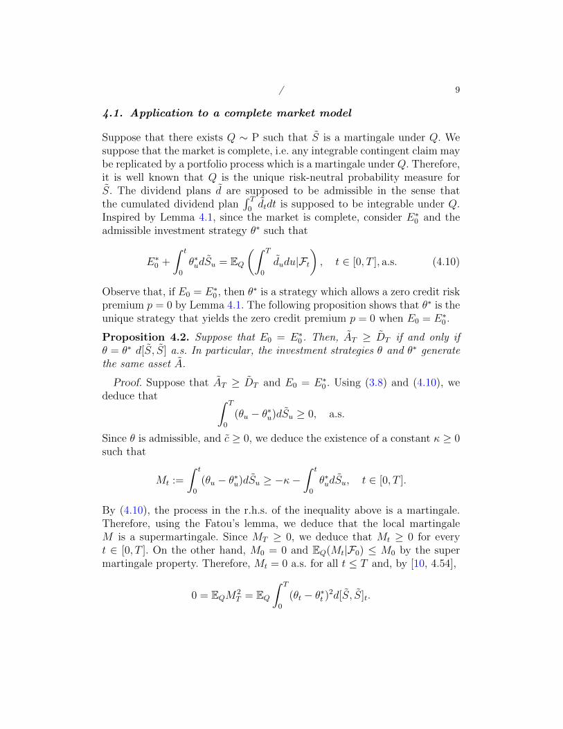
4.1. Application to a complete market model
Suppose that there exists Q ∼ P such that S is a martingale under Q. Wesuppose that the market is complete, i.e. any integrable contingent claim maybe replicated by a portfolio process which is a martingale under Q. Therefore,it is well known that Q is the unique risk-neutral probability measure forS. The dividend plans d are supposed to be admissible in the sense thatthe cumulated dividend plan
∫ T0dtdt is supposed to be integrable under Q.
Inspired by Lemma 4.1, since the market is complete, consider E∗0 and theadmissible investment strategy θ∗ such that
E∗0 +
∫ t
0
θ∗udSu = EQ(∫ T
0
dudu|Ft), t ∈ [0, T ], a.s. (4.10)
Observe that, if E0 = E∗0 , then θ∗ is a strategy which allows a zero credit riskpremium p = 0 by Lemma 4.1. The following proposition shows that θ∗ is theunique strategy that yields the zero credit premium p = 0 when E0 = E∗0 .
Proposition 4.2. Suppose that E0 = E∗0 . Then, AT ≥ DT if and only ifθ = θ∗ d[S, S] a.s. In particular, the investment strategies θ and θ∗ generatethe same asset A.
Proof. Suppose that AT ≥ DT and E0 = E∗0 . Using (3.8) and (4.10), wededuce that ∫ T
0
(θu − θ∗u)dSu ≥ 0, a.s.
Since θ is admissible, and c ≥ 0, we deduce the existence of a constant κ ≥ 0such that
Mt :=
∫ t
0
(θu − θ∗u)dSu ≥ −κ−∫ t
0
θ∗udSu, t ∈ [0, T ].
By (4.10), the process in the r.h.s. of the inequality above is a martingale.Therefore, using the Fatou’s lemma, we deduce that the local martingaleM is a supermartingale. Since MT ≥ 0, we deduce that Mt ≥ 0 for everyt ∈ [0, T ]. On the other hand, M0 = 0 and EQ(Mt|F0) ≤ M0 by the supermartingale property. Therefore, Mt = 0 a.s. for all t ≤ T and, by [10, 4.54],
0 = EQM2T = EQ
∫ T
0
(θt − θ∗t )2d[S, S]t.

/ 10
We deduce that θ = θ∗ d[S, S] a.s. Reciprocally, if this property holds, thenM = 0 hence (3.8) holds with p = 0. 2
Following the same arguments, we obtain the following general result:
Proposition 4.3. AT ≥ DT if and only if E0 ≥ E∗0 and
E0 +
∫ t
0
θudSu ≥ E∗0 +
∫ t
0
θ∗udSu, ∀t ∈ [0, T ].
Proof. As θ is supposed to be an admissible strategy, we deduce that thelocal martingale t 7→
∫ t0θudSu is a supermartingale. Therefore, with the in-
equality AT ≥ DT , i.e. (3.8), we obtain that:
E0 +
∫ t
0
θudSu ≥ E0 + EQ(∫ T
0
θudSu|Ft),
≥ EQ(∫ T
0
dudu|Ft),
≥ E∗0 +
∫ t
0
θ∗udSu.
With t = 0, we deduce that E0 ≥ E∗0 . This proposition above means thatthe debt holder should require a non null credit risk premium as soon as theinvestment strategy is not efficient enough or when the initial equity capitalis too small.
4.2. Valuation under the risk-neutral probability measure
In the following, we suppose that A ≥ 0. Let Q ∼ P be the risk-neutralprobability measure for S in the market model supposed to be complete. Inthe case of a possible default, e.g. when p 6= 0, the discounted payoff deliveredto the debt holders is
hDT :=
∫ T
0
ktDtdt+ AT ∧ DT , (4.11)
i.e. the sum of the cumulated amount of money reimbursed before T by thefirm and the residual debt DT when it is smaller than AT . Otherwise, in the
/ 11
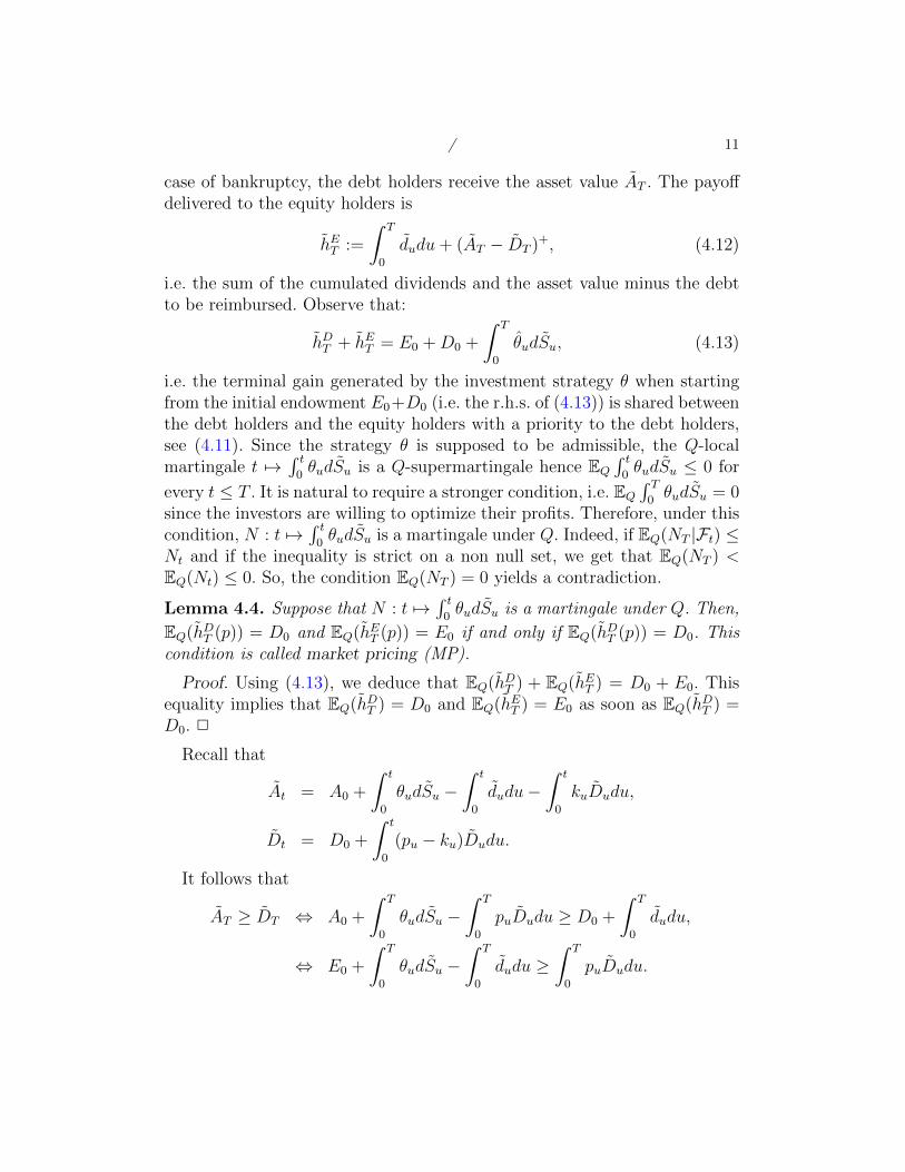
case of bankruptcy, the debt holders receive the asset value AT . The payoffdelivered to the equity holders is
hET :=
∫ T
0
dudu+ (AT − DT )+, (4.12)
i.e. the sum of the cumulated dividends and the asset value minus the debtto be reimbursed. Observe that:
hDT + hET = E0 +D0 +
∫ T
0
θudSu, (4.13)
i.e. the terminal gain generated by the investment strategy θ when startingfrom the initial endowment E0+D0 (i.e. the r.h.s. of (4.13)) is shared betweenthe debt holders and the equity holders with a priority to the debt holders,see (4.11). Since the strategy θ is supposed to be admissible, the Q-localmartingale t 7→
∫ t0θudSu is a Q-supermartingale hence EQ
∫ t0θudSu ≤ 0 for
every t ≤ T . It is natural to require a stronger condition, i.e. EQ∫ T0θudSu = 0
since the investors are willing to optimize their profits. Therefore, under thiscondition, N : t 7→
∫ t0θudSu is a martingale under Q. Indeed, if EQ(NT |Ft) ≤
Nt and if the inequality is strict on a non null set, we get that EQ(NT ) <EQ(Nt) ≤ 0. So, the condition EQ(NT ) = 0 yields a contradiction.
Lemma 4.4. Suppose that N : t 7→∫ t0θudSu is a martingale under Q. Then,
EQ(hDT (p)) = D0 and EQ(hET (p)) = E0 if and only if EQ(hDT (p)) = D0. Thiscondition is called market pricing (MP).
Proof. Using (4.13), we deduce that EQ(hDT ) + EQ(hET ) = D0 + E0. Thisequality implies that EQ(hDT ) = D0 and EQ(hET ) = E0 as soon as EQ(hDT ) =D0. 2
Recall that
At = A0 +
∫ t
0
θudSu −∫ t
0
dudu−∫ t
0
kuDudu,
Dt = D0 +
∫ t
0
(pu − ku)Dudu.
It follows that
AT ≥ DT ⇔ A0 +
∫ T
0
θudSu −∫ T
0
puDudu ≥ D0 +
∫ T
0
dudu,
⇔ E0 +
∫ T
0
θudSu −∫ T
0
dudu ≥∫ T
0
puDudu.
/ 12
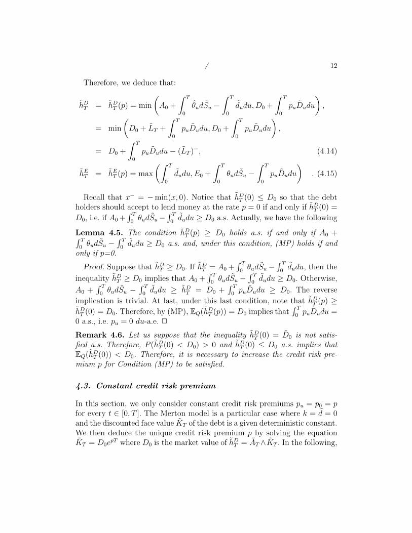
Therefore, we deduce that:
hDT = hDT (p) = min
(A0 +
∫ T
0
θudSu −∫ T
0
dudu,D0 +
∫ T
0
puDudu
),
= min
(D0 + LT +
∫ T
0
puDudu,D0 +
∫ T
0
puDudu
),
= D0 +
∫ T
0
puDudu− (LT )−, (4.14)
hET = hET (p) = max
(∫ T
0
dudu,E0 +
∫ T
0
θudSu −∫ T
0
puDudu
). (4.15)
Recall that x− = −min(x, 0). Notice that hDT (0) ≤ D0 so that the debtholders should accept to lend money at the rate p = 0 if and only if hDT (0) =
D0, i.e. if A0 +∫ T0θudSu−
∫ T0dudu ≥ D0 a.s. Actually, we have the following
Lemma 4.5. The condition hDT (p) ≥ D0 holds a.s. if and only if A0 +∫ T0θudSu −
∫ T0dudu ≥ D0 a.s. and, under this condition, (MP) holds if and
only if p=0.
Proof. Suppose that hDT ≥ D0. If hDT = A0 +∫ T0θudSu−
∫ T0dudu, then the
inequality hDT ≥ D0 implies that A0 +∫ T0θudSu −
∫ T0dudu ≥ D0. Otherwise,
A0 +∫ T0θudSu −
∫ T0dudu ≥ hDT = D0 +
∫ T0puDudu ≥ D0. The reverse
implication is trivial. At last, under this last condition, note that hDT (p) ≥hDT (0) = D0. Therefore, by (MP), EQ(hDT (p)) = D0 implies that
∫ T0puDudu =
0 a.s., i.e. pu = 0 du-a.e. 2
Remark 4.6. Let us suppose that the inequality hDT (0) = D0 is not satis-fied a.s. Therefore, P (hDT (0) < D0) > 0 and hDT (0) ≤ D0 a.s. implies thatEQ(hDT (0)) < D0. Therefore, it is necessary to increase the credit risk pre-mium p for Condition (MP) to be satisfied.
4.3. Constant credit risk premium
In this section, we only consider constant credit risk premiums pu = p0 = pfor every t ∈ [0, T ]. The Merton model is a particular case where k = d = 0and the discounted face value KT of the debt is a given deterministic constant.We then deduce the unique credit risk premium p by solving the equationKT = D0e
pT where D0 is the market value of hDT = AT ∧KT . In the following,

/ 13
we show the uniqueness of such a constant credit risk premium for our model
in the case where EQ(∫ T
0drdt
)< E0. Notice that, if this inequality does not
hold, there is no economical reason for the debt holders to lend money as thefirm is not solvent (see Lemma below) even if the condition (MP) actuallyholds whatever p. In that case, we take the convention that the credit riskprime is p∗ = 0 as hDT (p) does not depend on p.
Proposition 4.7. Suppose that EQ(∫ T
0drdt
)≥ E0. Then, EQ(hDT (p)) ≥ D0
if and only if EQ(∫ T
0drdt
)= E0, and LT = AT − DT ≤ 0 a.s. i.e.
E0 +
∫ T
0
θudSu −∫ T
0
dudu ≤∫ T
0
puDudu, a.s.
Under these conditions, hDT (p) does not depend on p and EQ(hDT (p)) = D0.
Proof. By (4.14), EQ(hDT (p)) ≥ D0 if and only if
EQ((LT )−) ≤ EQ(∫ T
0
puDudu
)or equivalently if
EQ
((∫ T
0
puDudu− γ)+)≤ EQ
(∫ T
0
puDudu
),
where
γ = L0 +
∫ T
0
θudSu −∫ T
0
dudu = LT +
∫ T
0
puDudu.
Since x+ ≥ x, we deduce that
EQ
((∫ T
0
puDudu− γ)+)≥ EQ
(∫ T
0
puDudu
)− EQ(γ).
Since L0 = E0 and EQ(∫ T
0drdt
)≥ E0, then EQ(γ) ≤ 0. It follows that
EQ(hDT (p)) ≥ D0 if and only if EQ(γ) = 0, i.e. EQ(∫ T
0drdt
)= E0, and
EQ
((∫ T
0
puDudu− γ)+)
= EQ(∫ T
0
puDudu
).
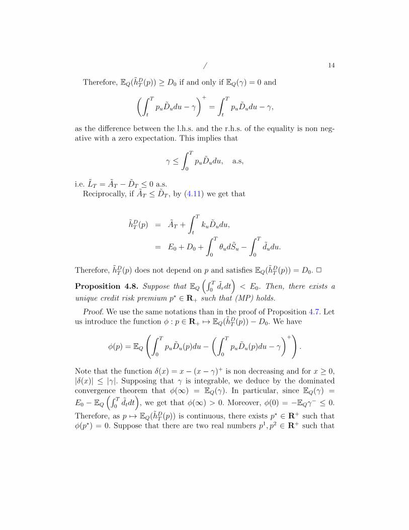
/ 14
Therefore, EQ(hDT (p)) ≥ D0 if and only if EQ(γ) = 0 and(∫ T
t
puDudu− γ)+
=
∫ T
t
puDudu− γ,
as the difference between the l.h.s. and the r.h.s. of the equality is non neg-ative with a zero expectation. This implies that
γ ≤∫ T
0
puDudu, a.s,
i.e. LT = AT − DT ≤ 0 a.s.Reciprocally, if AT ≤ DT , by (4.11) we get that
hDT (p) = AT +
∫ T
t
kuDudu,
= E0 +D0 +
∫ T
0
θudSu −∫ T
0
dudu.
Therefore, hDT (p) does not depend on p and satisfies EQ(hDT (p)) = D0. 2
Proposition 4.8. Suppose that EQ(∫ T
0drdt
)< E0. Then, there exists a
unique credit risk premium p∗ ∈ R+ such that (MP) holds.
Proof. We use the same notations than in the proof of Proposition 4.7. Letus introduce the function φ : p ∈ R+ 7→ EQ(hDT (p))−D0. We have
φ(p) = EQ
(∫ T
0
puDu(p)du−(∫ T
0
puDu(p)du− γ)+).
Note that the function δ(x) = x− (x− γ)+ is non decreasing and for x ≥ 0,|δ(x)| ≤ |γ|. Supposing that γ is integrable, we deduce by the dominatedconvergence theorem that φ(∞) = EQ(γ). In particular, since EQ(γ) =
E0 − EQ(∫ T
0dtdt
), we get that φ(∞) > 0. Moreover, φ(0) = −EQγ− ≤ 0.
Therefore, as p 7→ EQ(hDT (p)) is continuous, there exists p∗ ∈ R+ such thatφ(p∗) = 0. Suppose that there are two real numbers p1, p2 ∈ R+ such that
/ 15
φ(p1) = φ(p2) = 0 and p1 < p2. Since δ is strictly increasing on (−∞, γ) andconstant on [γ,∞), we obtain that
δ
(∫ T
0
p1Du(p1)du
)≤ δ
(∫ T
0
p2Du(p2)du
)and, finally, the equality holds due to the assumption. Therefore, we neces-sarily have ∫ T
0
p2Du(p2)du ≥ γ
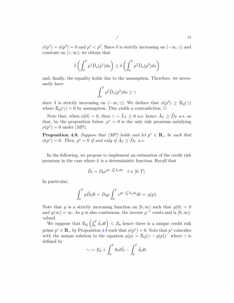
since δ is strictly increasing on (−∞, γ). We deduce that φ(p2) ≥ EQ(γ)where EQ(γ) > 0 by assumption. This yields a contradiction. 2
Note that, when φ(0) = 0, then γ = LT ≥ 0 a.s. hence AT ≥ DT a.s. sothat, by the proposition below, p∗ = 0 is the only risk premium satisfyingφ(p∗) = 0 under (MP).
Proposition 4.9. Suppose that (MP) holds and let p∗ ∈ R+ be such thatφ(p∗) = 0. Then, p∗ = 0 if and only if AT ≥ DT a.s.
In the following, we propose to implement an estimation of the credit riskpremium in the case where k is a deterministic function. Recall that
Dt = D0ept−
∫ t0 kudu t ∈ [0, T ].
In particular, ∫ T
0
pDtdt = D0p
∫ T
0
ept−∫ t0 kududt =: g(p).
Note that g is a strictly increasing function on [0,∞) such that g(0) = 0and g(∞) =∞. As g is also continuous, the inverse g−1 exists and is [0,∞)-valued.
We suppose that EQ(∫ T
0drdt
)< E0 hence there is a unique credit risk
prime p∗ ∈ R+ by Proposition 4.8 such that φ(p∗) = 0. Note that p∗ coincideswith the unique solution to the equation g(p) = EQ(γ − g(p))− where γ isdefined by
γ := E0 +
∫ T
0
θtdSt −∫ T
0
dtdt.

/ 16
Here, we suppose that γ is square integrable. Let us consider the sequencepn defined by p0 = 0 and
pn+1 = g−1(EQ(γ − g(pn))−
),
i.e. g(pn+1) = EQ(γ − g(pn))−. As p0 = 0, we have p1 ≥ p0. Since g isincreasing and x 7→ x− is non decreasing, we may show by induction thatpn+1 ≥ pn for all n ≥ 0. Similarly, as p0 ≤ p∗, we deduce that g(p1) ≤EQ(γ − g(p∗))− = g(p∗) hence p1 ≤ p∗ and, by induction, pn ≤ p∗ for alln ≥ 0. We finally deduce that the increasing sequence (pn)n converges to p∗.
In practice, it seems to be difficult to implement the iteration schemepn+1 = g−1 (EQ(γ − g(pn))−) as we need first to estimate the expectation of(γ − g(pn))−. Note that, since g is invertible, the problem is equivalent tosolve the equation x = EQ(γ − x)− whose solution is x∗ = g(p∗) so thatp∗ = g−1(x∗). Clearly x∗ does not depend on D0 while p∗ does as it is thesolution to the equation x∗ = g(p∗).
In order to estimate x∗, we propose a method inspired by the well knownstochastic gradient descent. Precisely, we consider a sequence (γn)n≥1 of in-dependent random variables distributed as γ and we introduce the followingscheme: x1 = 0 and
xk+1 = xk − αkH(γk, xk), k ≥ 0,
where H(v, x) = x − (v − x)−, and (αk)k≥1 is a positive sequence satisfying∑∞k=1 αk = +∞ and
∑∞k=1(αk)
2 < +∞.
Theorem 4.10. The sequence (xk)k≥1 converges a.s. to x∗.
Proof. Note that H(v, x) = x1x≤v + v1x>γ, in particular x 7→ H(γ, x) isnon decreasing. Let us define the non decreasing function C(x) = EH(γ, x).We have C(0) = −EQγ− and C(∞) = EQγ > 0 by assumption. Recall alsothat C(x∗) = 0 by assumption. Since γ is integrable, we also deduce that Cis continuous. Therefore, as C is non decreasing and the equation C(x) = 0admits a unique solution, we deduce that, for every ε > 0,
inf|x−x∗|>ε
(x− x∗)C(x) > 0. (4.16)

/ 17
On the other hand, let us introduce D(x) = EQH2(γ, x). We have
D(x) = EQ (H(x, γ)−H(x∗, γ) +H(x∗, γ))2 ,
≤ 2EQ (H(x, γ)−H(x∗, γ))2 + 2EQH2(x∗, γ),
≤ 8(x− x∗)2 + 2EQγ2.
The last inequality is deduced from the fact that H(·, γ) is 2-Lipschitz andthat |H(x, γ)| ≤ |γ| if x ≥ 0.
Let us introduce the sequence dk = (xk − x∗)2, k ≥ 1 and the filtrationFk = σ(γ1, · · · , γk−1), k ≥ 2, and F1 is the trivial σ-algebra induced by thenegligible sets. Notice that xk ∈ L0(R,Fk) for all k. The goal is to show thatdk converges a.s. to zero. To do so, let us first compute
dk+1 − dk = (xk+1 − x∗)2 − (xk − x∗)2 = (xk − αkH(γk, xk)− x∗)2 − (xk − x∗)2,dk+1 − dk = α2
kH2(γk, xk)− 2αkH(γk, xk)(xk − x∗).
We deduce that
E(dk+1 − dk|Fk) = α2kEQ
(H2(γk, xk)|Fk
)− 2αk(xk − x∗)EQ (H(γk, xk)|Fk) .
As γk is independent of Fk and xk is Fk-measurable, we deduce that
EQ(H2(γk, xk)|Fk
)= EQ
(H2(γ, xk)
), EQ (H(γk, xk)|Fk) = EQ (H(γ, xk)) .
Therefore, by the first step,
EQ(dk+1 − dk|Fk) ≤ 8α2k(xk − x∗)2 + 2α2
kEQγ2 − 2αk(xk − x∗)EQ (H(γ, xk)) . (4.17)
Therefore, as αk(xk − x∗)EQ (H(γ, xk)) ≥ 0,
EQ(dk+1 − dk(1 + 8α2k)|Fk) ≤ 2α2
kEQγ2. (4.18)
Let us introduce δk+1 = µkdk+1, k ≥ 0, where µk := Πk−1j=1(1+8α2
k)−1, k ≥ 1
and µ0 = 1. Multiplying (4.18) by µk, we obtain that
EQ(δk+1 − δk|Fk) ≤ 2α2kµkEQγ2. (4.19)
From above, we deduce that the process Mk := δk − 2EQγ2∑k
j=1 α2kµk,
k ≥ 1, is a super martingale. As δk ≥ 0 for all k ≥ 1, M is bounded from

/ 18
above hence (Mk)k≥1 is a.s. convergent by the Doob’s theorem. We deducethat (δk)k≥1 is also convergent. As the sequence (ln(µk))k≥1 is convergent, wededuce that µk → µ > 0 hence the sequence dk = (xk − x∗)2 is convergent.
Taking the expectation in (4.17) and summing up, as dk ≥ 0, we get that
EQ
(∞∑k=1
αk(xk − x∗)EQ (H(γ, xk))
)<∞,
and finally
0 ≤∞∑k=1
αk(xk − x∗)EQ (H(γ, xk)) <∞,
where we recall that αk(xk − x∗)EQ (H(γ, xk)) ≥ 0 a.s. for all k ≥ 1.Let us define r = lim infk→∞(xk − x∗)EQ (H(γ, xk)). Suppose that r > 0.
Then, (xk − x∗)EQ (H(γ, xk)) > r/2 for k ≥ k0 large enough so that
∞∑k=k0
αk(xk − x∗)EQ (H(γ, xk)) > r/2∞∑
k=k0
αk = +∞,
which yields a contradiction. We deduce that r = 0 and, in the case wherelimk→∞ dk = 2ε2 > 0, we get that (xk − x∗)2 ≥ ε2 for k large enough. By(4.16), we deduce a constant c such that (xk − x∗)C(xk) > c where we recallthat C(xk) = EQ (H(γ, xk)) hence a contradiction, i.e. limk→∞ dk = 0. 2
5. Conclusion
We consider the problem of characterizing and computing the fair credit riskpremium that a non-financial firm should pay when borrowing money froma bank. In particular, we study the case where the risk premium dependsexplicitly on the firm’s strategy such that the expected discounted valueof the bank’s payoff coincides with the loan’s par value. The strategy isexplicitly defined in terms of investment and consumption. We use a risk-neutral framework to show the existence of a unique credit risk premium forsuch a commercial loan. We then propose a numerical procedure to estimatethe fair premium. A limit of this research is that it relies on the assumptionof the absence of information asymmetry between the bank and the non-financial firm, which suggests a new direction for further research.
/ 19
References
[1] Allen B.N., Scott, F.W., and Vasso, I. 2016. Reexamining the empiricalrelation between loan risk and collateral: The roles of collateral liquidityand types. Journal of Financial Intermediation, 26, 28-46.
[2] Berg, T., Saunders,A., Steffen, S., and Streitz, D. 2017. Mind the Gap:The Difference between U.S. and European Loan Rates, The Reviewof Financial Studies, 30, 3, 948-987.
[3] Blochlinger, A., 2018, Credit Rating and Pricing: Poles Apart. Journalof Risk and Financial Management, 11, 2, 27.
[4] Bouchard, B., Elie, R., and Imbert, C. Optimal Control under Stochas-tic Target Constraints
[5] Culp, C.L., Nozawa, Y., and Veronesi, P. 2018. Option-Based CreditSpreads. American Economic Review, 108, 2, 454-88.
[6] Duffie, D., and Lando, D. 2001. Term Structures of Credit Spreads withIncomplete Accounting Information. Econometrica, 69, 633-664.
[7] Eom, Y. H., J., Helwege, and Huang, J.-z. 2004. Structural modelsof corporate bond pricing: An empirical analysis. Review of FinancialStudies, 17, 2, 499-544.
[8] Giesecke, K., Longstaff, F.A., Schaefer, S., and Strebulaev, I. 2011. Cor-porate bond default risk: A 150-year perspective. Journal of FinancialEconomics 102(2), 233-250.
[9] Huang, J.Z., and Huang, M. 2012. How much of the corporate-treasuryyield spread is due to credit risk? Review of Asset Pricing Studies, 2,2, 153-202.
[10] Jacod J., and Shiryaev, A.N. Limit Theorems for Stochastic Processes.Springer, Berlin–Heidelberg–New York, 1987.
[11] Kuehn, L., and Schmid, L. 2014. Investment-Based Corporate BondPricing. The Journal of Finance, 69, 2741-2776.
[12] Leland, H.E., and Toft, K.B. 1996. Optimal Capital Structure, Endoge-nous Bankruptcy, and the Term Structure of Credit Spreads. Journalof Finance, 51, 3, 987-1019.
[13] Leland, H.E. 1998. Agency Costs, Risk Management, and CapitalStructure. Journal of Finance, 53, 4, 1213-1243.
[14] Lee S.J., Liu, L.Q., and Stebunovs, V. 2017. Risk Taking and InterestRates: Evidence from Decades in the Global Syndicated Loan Mar-ket,IMF Working Paper.
[15] Liu, L-C., Dai, T.-S., and Wang, C.-J. 2016. Evaluating corporate
/ 20
bonds and analyzing claim holders’ decisions with complex debt struc-ture, Journal of Banking & Finance, 72, 151-174.
[16] Modigliani, F., and Miller, M.H. 1958. The cost of capital, corporationfinance and the theory of investment. American economic review 48, 3,261-297.
[17] Papin, T. 2013. Pricing of Corporate Loan: Credit Risk and Liquiditycost. Working paper, University of Paris-Dauphine.
[18] Santos, J.A.C., 2011. Bank Corporate Loan Pricing Following the Sub-prime Crisis, The Review of Financial Studies, 24, 6, 1916-1943.
[19] Schwert, M. 2018. Is Borrowing from Banks More Expensive than Bor-rowing from the Market? Working Paper, The Ohio State University.