Embed Size (px)
Citation preview

EVALUATION OF THE COST EFFECTIVENESS OF THE
1983 STREAM-GAGING PROGRAM IN KANSAS
By K. D. Medina and C. 0. Geiger
U.S. GEOLOGICAL SURVEY
Water-Resources Investigations Report 84-4107
Prepared in cooperation with the
KANSAS WATER OFFICE
Lawrence, Kansas
1984

UNITED STATES DEPARTMENT OF THE INTERIOR
WILLIAM P. CLARK, Secretary
GEOLOGICAL SURVEY
Dallas L. Peck, Director
For additional write to:
information
District ChiefU.S. Geological Survey, WRD1950 Constant Avenue - Campus WestUniversity of KansasLawrence, Kansas 66044-3897[Telephone: (913) 864-4321]
Copies of this report can be purchased from:
Open-File Services Section Western Distribution Branch U.S. Geological Survey Box 25425, Federal Center Lakewood, Colorado 80225 [Telephone: (303) 234-5888]

CONTENTS
Page
Abstract................................................................ 1Introduction............................................................ 1
History of stream-gaging program in Kansas......................... 2Stream-gaging program in Kansas, 1983.............................. 4
Data uses, funding, and availability from stream-gaging program......... 4Data-use categories................................................ 4
Regi onal hydro!ogy............................................ 4Hydro!ogi c systems............................................ 5Legal obiigations............................................. 5Planning and design........................................... 5Project operation............................................. 23Hydrologi c forecasts.......................................... 23Water-qua!ity monitoring...................................... 23Research...................................................... 24Other......................................................... 24
Funding............................................................ 24Frequency of data availability..................................... 25Plans for future program evaluation................................ 25
Alternative methods of developing streamflow information................ 25Discussion of methods.............................................. 26
Regression analysis........................................... 26Categorization of stream gages by their potential for
alternative methods.............................................. 27Results of regression analysis...................................... 28
Cost-effective resource allocation....................................... 29Kalman filtering for cost-effective resource allocation (K-CERA).... 29
Description of mathematical program............................ 30Description of uncertainty functions........................... 32
Application of K-CERA in Kansas..................................... 36Definition of missing-record probabilities..................... 37Definition of cross-correlation coefficient and
coefficient of variation..................................... 37Kalman-filtering definition of variance........................ 38K-CERA results................................................. 43
Summary.................................................................. 55References cited......................................................... 56
ILLUSTRATIONS Figure Page
1. Graph showing number of complete-record, streamflow-gagingstations in operation in Kansas, water years 1895-1983.......... 3
2. Map of Kansas showing area of program responsibility and location of complete-record, streamflow-gaging stations, water year 1983................................................. 6
3. Mathematical-programing form for optimization of hydro-grapher routing................................................. 31
iii

ILLUSTRATIONS Continued
Figure Page
4. Tabular form for optimization of hydrographer routing........... 32
5. Graph showing typical uncertainty functions for instantaneousdi scharge..................................................... 42
6. Graph showing temporal, average standard error per streamgage.......................................................... 44
TABLES Table Page
1. Selected hydro!ogic data from complete-record stationsin the 1983 Kansas stream-gaging program...................... 8
2. Data use, funding, and frequency of data availability for complete-record stations in the 1983 Kansas stream-gaging program....................................................... 16
3. Combination of stations used in regression analysis............. 28
4. Summary of autocovariance analysis and coefficient ofvariation..................................................... 39
5. Selected results of K-CERA analysis............................. 46
CONVERSION TABLE
Factors for converting the inch-pound units given in this report to the International System (SI) of Units are given below:
Multiply inch-pound unit By To obtain SI units
Length
mile 1.609 kilometer
Area
square mile 2.590 square kilometer
Vo!ume
cubic foot 0.02832 cubic meter
Flow
cubic foot per second 0.02832 cubic meter per second
IV

EVALUATION OF THE COST EFFECTIVENESS OF THE 1983
STREAM-GAGING PROGRAM IN KANSAS
by K. D. Medina and C. 0. Geiger
ABSTRACT
This report documents the results of an evaluation of the cost effec tiveness of the 1983 stream-gaging program in Kansas. Data uses and funding sources were identified for the 140 complete-record, streamf low-gaging stations operated in Kansas during 1983 with a budget of $793,780. As a result of the evaluation of the needs and uses of data from the stream- gaging program, it was found that the 140 gaging stations were needed to meet these data requirements.
The average standard error of estimate for records of instantaneous discharge was 21 percent, assuming the 1983 budget and operating schedule of 6-week interval visitations and based on 85 of the 140 stations. It was shown that this overall degree of accuracy could be improved to 19 percent by altering the 1983 schedule of station visitations. A minimum budget of $760,000, with a corresponding average standard error of estimate of 25 percent, is required to operate the 1983 program; a budget of less than this would not permit proper service and maintenance of the stations or adequate definition of stage-discharge relations. The maximum budget analyzed was $1,191,000, which resulted in an average standard error of estimate of 9 percent.
None of the stations investigated were suitable for the application of alternative methods for simulating discharge records. Improved instru mentation can have a very positive impact on streamflow uncertainties by decreasing lost record.
INTRODUCTION
The U.S. Geological Survey is the principal Federal agency collecting surface-water data in the Nation. The data are collected in cooperation with State and local governments and with other Federal agencies. The Survey is presently (1983) operating approximately 8,000 complete-record, streamflow-gaging stations throughout the Nation. Some of these records extend back to the turn of the 20th century. Any activity of long standing, such as the collection of surface-water data, needs to be re-examined at in tervals, if not continuously, because of changes in objectives, technology, or external constraints. The last systematic, nationwide evaluation of the streamflow-information program was completed in 1^70 and is documented by Benson and Carter (1973). The Survey is presently (1983) undertaking another nationwide evaluation of the stream-gaging program that will be completed during 5 years with 20 percent of the program being analyzed each year on a State-by-State basis. The objective of this evalution is to define and document the most cost-effective means of providing stream- flow information.
1

For Kansas, a major part of the evaluation was done in cooperation with the Kansas Water Office (formerly the Kansas Water Resources Board), which is the principal State agency supporting the Kansas stream-gaging program.
For every complete-record gaging station, the evaluation identified the principal uses of the data and related these uses to funding sources. In addition, gaging stations were categorized as to whether the data were available to users by telemetry for immediate use, by release on a provi sional basis, or at the end of the water year.
The second part of this evaluation was to identify less costly alter native methods of providing the needed information. Among these methods are streamflow-routing models and statistical analysis. The Kansas stream- gaging program no longer is considered as a network of observation points, but rather as an integrated information system in which data are provided both by observation and synthesis.
The final part of the evaluation involved the use of Kalman-filtering and mathematical-programing techniques to define strategies for operation of the necessary stations that minimized the uncertainty in the streamflow records for given operating budgets. Kalman-filtering techniques (Moss and Gilroy, 1980) were used to compute uncertainty functions by relating the standard errors of computation or estimation of streamflow records to the frequencies of visits to the stream gages for all stations in the analysis. A steepest-descent optimization program used these uncertainty functions, information on practical stream-gaging routes, the various costs associated with stream gaging, and the total operating budget to identify the visit frequency for each station that minimized the overall uncertainty in the streamflow record. A stream-gaging program that resulted from this evalu ation should meet the expressed water-data needs in the most cost-effective manner.
This report is organized into five sections, the first being an intro duction to the stream-gaging activities in Kansas and to the study itself. The middle three sections each contain discussions of individual parts of the evaluation. The study is summarized in the final section.
History of Stream-Gaging Program in Kansas
A graphic history of the number of complete-record, streamflow-gaging stations in operation in Kansas since water year 1895 is shown in figure 1. The records from these stations consist of daily streamflows obtained from operation at selected sites. Only a few records were collected until about 1920 (fig. 1), when several new stations began operation, and an effort was made to establish a more permanent and continuous data-collection program. There was a further expansion beginning in about 1940, when addi tional stream-gaging stations were started in an attempt to define areal variations in streamflow, to collect data specifically required by Federal agencies, to manage water supplies, and to define the magnitude and frequency of floods in critical areas.

NU
MB
ER
O
F C
OM
PL
ET
E-R
EC
OR
D.
ST
RE
AM
FL
OW
-GA
GIN
G
ST
AT
ION
S
IN O
PE
RA
TIO
N
(O -J fD 3
cr
fD -5 ri-
ro fD
O
O O-
fD fD
o>
to
s 00 3
C
O to to
rl
-
rl-
O
co 3
O fD -J
O
O
-h
-h O
o
fD
fD
Q)
rt I
co
rl-
3
3-
3"
fD
fD
co
fD
fDI
O>
.-
~J
tO ,
7^
Oi
^
to O
l ro
*"
n- ^
o
2:O
> '
O)
co
rt ^
O
rl
-
O-
O*
e ?
* ^
CO
3
~.
Oro
to ;
0-
/-»
CT i
CD
-<
3-
fDQ
- -
*<
cu
i"1"^
-j
o
co c
i.
fD
O
g-
-,
3
rr
<~>
.2 -"
< <
5 ro
-S e_
g.
~*
ro
Cj
to r
oO
O
-s^J
~_
P ~
^ iD
o- i
' S-
° °
-
fD 3
^
Q
-^
3
T-
fP
pi
n- r
o CD
t<
Oi
*"*" 3
'
O I
Q)
C
OI
_K 3
CU
O
m S
*
O.
fD
O>
CO
n-
fD
"^ T
-J.
<
OO
O
O
fD "
O
tO3
O
-1
-1CO
3
O>
O>
O>
fD
' 3
3
»
T *
**
fD
fD
«^ o r
ofD
Q-
-1
C
fD
~5
"O
-1-
O
U3
rl-
3-
3
Q>
3
O.
en c
*>J
~5 3
O>
fD
3
CO
OL
to
CO
O
> LO
'
n-
n- -
-i
o
o>
tofD
O
rl
- 3
-o>
o
-"
3 -
o o
n--h
fD
3
3"-
-1
fD
o
o> - I f
D
O
<
3- i
3"
fD
fD
O>
O>
rl-
3
fD-h
O
O
O33 1
n- N
fD
-J.
fD
O
O- 3
3
fD
O>
fD-£.
cr
o.
PI
Qto
c:
_K
fD
H->
10
vo
o>
cn~
*j
"*^J
o ^
fD
Q)
O
rl-
fDO
00 3
,t'
3
ro
"rl
- 2i
-J-J
- n-
o §
o
o t
o x
CO
_
i. O
/^
l "^
o
1,.
o
=
o-
<3
5 rl-
CD rl-
O.
-h
O
^* "
O
C7"
co
-j
rl-
O
O
O> -13
O,
-j.
*<
3
3fD
C
QO
> O
-l
-h rl
- 3
"i
' co
fD
<>D
rl-
CT> I
oO
fD
Q
,
3 ST
fD
3-
" 54
3CO
fD
C
O O
3
'
rl-
O>
co 3
-i
3
-
fD
O
-+,
O
Si
o
fD
O
fD 3
S
fD
CO
jli
c^"
S fD
to
O>
<-!
n- -
'fD
3
Q.C
Q
O 3"
O-
o>
rl-
O>
O>
o
cr -
' _,
. -b
fD
n- -
3 fD
n-
(/~
o>CO
fD
ofD
_i
.j.
n-
3
-
fDfD
3
O>
fD
S:
fD 3
O-
3-
Q-
-h
Q-
O
-
O<
3- 3
s:
«O
Q
L O
-"5
5H
. fD
O
<"
CO
O>n-
ocu
CQ
s:
cr -
o
> i
o
to

As shown in figure 1, an increase in the number of complete-record stations occurred during 1980. This was the result of a substantial in crease in the number of stations operated for specific project information. These stations subsequently have been discontinued, and the level of opera tion now has returned to a network similar to that of the mid-1970's.
Stream-Gaging Program in Kansas, 1983
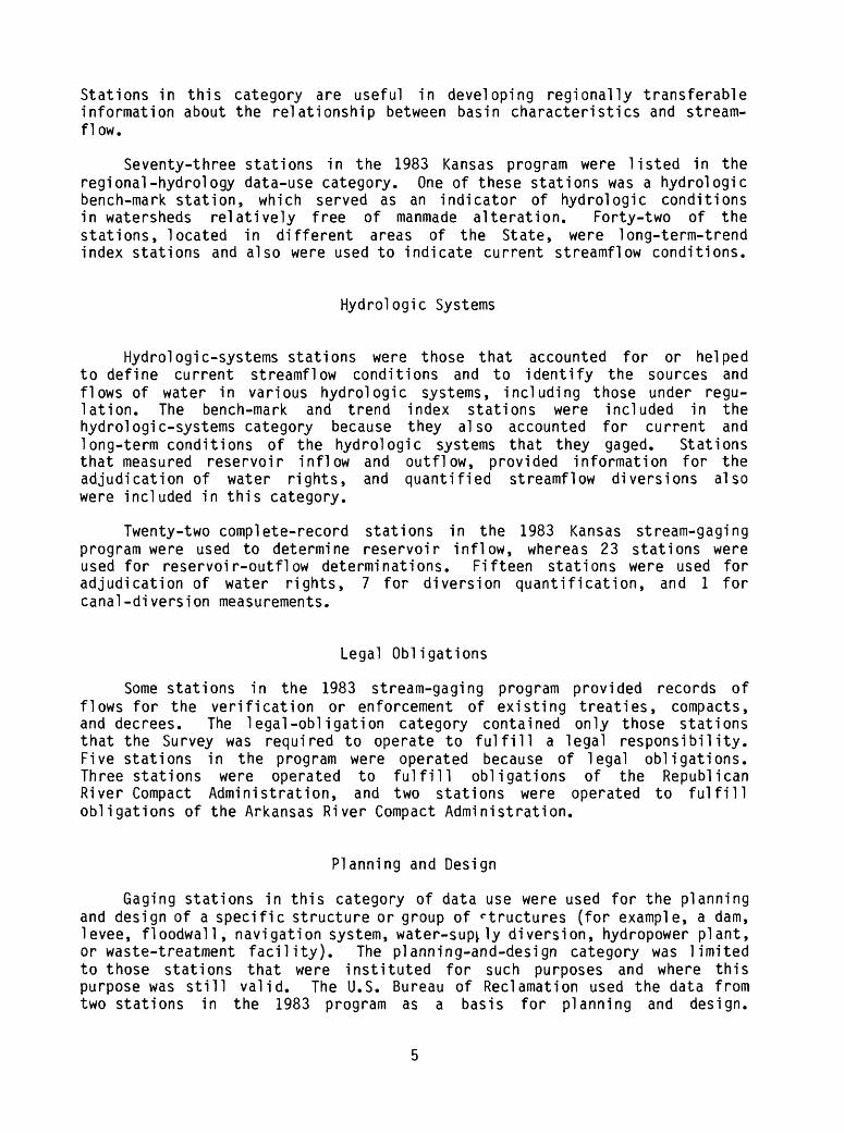
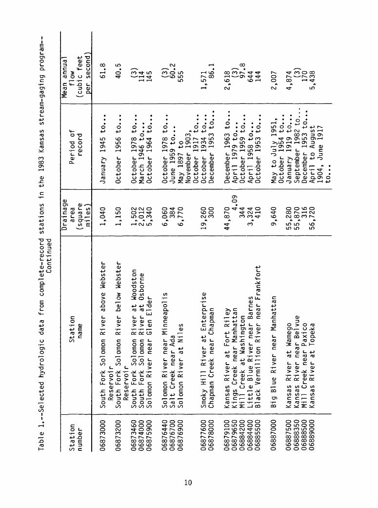
The stream-gaging program in Kansas is operated and maintained from two offices of the Geological Survey, a Subdistrict office in Garden City and a Field Headquarters office in Lawrence, which also is the location of the District office. The general area of responsibility for 1983 program operation, as well as the location and distribution of the 140 complete- record stations, is shown in figure 2. The 1983 program also included systematic collection of information on annual peak discharge, seasonal pre cipitation, river stage, and reservoir contents at 137 additional sites in the State. The U.S. Geological Survey number and name for each complete- record gaging station in the 1983 stream-gaging program, as well as selected hydrologic data that include drainage area, period of record, and mean annual flow, are given in table 1. Station-identification numbers used throughout this report are based on a downstream-order numbering system used by the Survey.
DATA USES, FUNDING, AND AVAILABILITY FROM STREAM-GAGING PROGRAM
Data-Use Categories
The relevance of a gaging station is defined by the uses that are made of the data collected at the station. The data uses from each complete- record station in the 1983 Kansas program were identified by a survey of known data users. The survey documented the importance of each station and provided for the identification of those gaging stations that could be con sidered for discontinuation. Data-use and ancillary information are pre sented for each complete-record station in table 2, which contains an ex planation on each page to expand the information conveyed. The entry of an asterisk in the table indicates that no additional explanation is required. Data uses identified by the survey were placed in the nine categories defined below.
Regional Hydrology
For streamflow data to be useful in defining regional hydrology, a stream must be largely unaffected by manmade storage or diversion. In this category of use, the effects of man on streamflow are not necessarily insignificant, but the effects are limited to those caused primarily by land use and climatic changes. Large quantities of manmade storage can occur in the basin, providing the outflow from storage is uncontrolled.
Stations in this category are useful in developing regionally transferable information about the relationship between basin characteristics and stream- flow.
Seventy-three stations in the 1983 Kansas program were listed in the regional-hydrology data-use category. One of these stations was a hydro!ogic bench-mark station, which served as an indicator of hydrologic conditions in watersheds relatively free of manmade alteration. Forty-two of the stations, located in different areas of the State, were long-term-trend index stations and also were used to indicate current streamflow conditions.
Hydrologic Systems
Hydrologic-systems stations were those that accounted for or helped to define current streamflow conditions and to identify the sources and flows of water in various hydrologic systems, including those under regu lation. The bench-mark and trend index stations were included in the hydrologic-systems category because they also accounted for current and long-term conditions of the hydrologic systems that they gaged. Stations that measured reservoir inflow and outflow, provided information for the adjudication of water rights, and quantified streamflow diversions also were included in this category.
Twenty-two complete-record stations in the 1983 Kansas stream-gaging program were used to determine reservoir inflow, whereas 23 stations were used for reservoir-outflow determinations. Fifteen stations were used for adjudication of water rights, 7 for diversion quantification, and 1 for canal-diversion measurements.
Legal Obligations
Some stations in the 1983 stream-gaging program provided records of flows for the verification or enforcement of existing treaties, compacts, and decrees. The legal-obligation category contained only those stations that the Survey was required to operate to fulfill a legal responsibility. Five stations in the program were operated because of legal obligations. Three stations were operated to fulfill obligations of the Republican River Compact Administration, and two stations were operated to fulfill obligations of the Arkansas River Compact Administration.
Planning and Design
Gaging stations in this category of data use were used for the planning and design of a specific structure or group of c tructures (for example, a dam, levee, floodwall, navigation system, water-supply diversion, hydropower plant, or waste-treatment facility). The planning-and-design category was limited to those stations that were instituted for such purposes and where this purpose was still valid. The U.S. Bureau of Reclamation used the data from two stations in the 1983 program as a basis for planning and design.

102° 101° 100° 99° 98°
1 II10° - - - _ _ __ ______.. 1
4846500 T A848500
848000CHEYENNE , DECATUR jftjiP PHIUIPS
i - ' » 8479wv/ sn + nnn' RAWIiru<; A OY IVJUU
1
1 8538001 A "^»4} 854000
SMITH JEWELL
1
844900 fl-7^c«/>^871800 i 871500 r , | A' 87250^0^^5900
^v 873200 A A "r^*i Gooriand SHERIDAN 8730004^^* 873460 874000) MITCHELL
A8447OO GRAHAM ROOKS, SHERMAN y-»-" "W
THOMAS
1 . 866900
"' | , 485850ft _LOGAN
| WALLACE , , ' GOVE TREGO ' 8 639 00 8
A 891000A ~&££&QQ A. 860000 ' T * 863500
f ^ l 6 862700 A8628 ''x " ^ -' ' _-^ ' " " ~~^^ ''"^^'' /
OSBORNE |
1
1 ,
^_ 868^00 I^-^~^^^^^ LINCOLN!
67QM^^ !864050 1
664500 J 50 A "^
^^^ . . __^ .. _ J_LLSWORTH!J*
I " r~~ " ' ~~^ ' " HVSH~~^A'lt*nn BARTON ^^ U_GREELEr lOQ^c'rt 11* SCOTT ' NESS 141900 *~i loo 6 50 LANE , v\ A *
141780f
I A 141200
/j37,aftQN HODGEMAl 40850 PAWNEE
30° JM 37500 KEARNY FINNE »
138000 -^ 1400001 s / ^ EDWARDS
139500 '
A156220 FQRO'^'1 ' GRANT ' >
j' "TiSelOO % HASKEU ' 139800 KIDWA
I ' ' " . .I - f.'-
Al56ft10 MEADE .......
MORTON STEVENS
A155590 SEWARO
I?'-^--- -- ,-__ .. _ _ 4157500
A 143300141300 i«, AA''S,
142620 LSTAFFORD » '
142575
RENO
A142300
PRATT
A144910 KINGMAN
BARBER HARPE "
149£00
I i " "I " "" ""102° 101- 100° 99 90°
EXPLANATION
BOUNDARY OF PROGRAM RESPONSIBILITY
A 887500 COMPLETE-RECORD STATION AND NUMBER
BASIN BOUNDARY
7 ARKANSAS RIVER BASIN
6 MISSOURI RIVER BASIN
@ DISTRICT OFFICE AND LAWRENCE FIELD HEADQUARTERS
® GARDEN CITY SUBDISTRICT OFFICE

853500
REPUBLIC
855800 A A856000
884200 MARSHALLA
WASHINGTON
88440(
814000 BROVVN
NEMAHA DONIPHAN
4WX« .. *T» ATCHISON*889140 Q A889160\
?7<}?°0 877*600WABAUNSEE
QUOTAS
^A8655OO
911 900
893300 JOHNSON ^
893Q80
179500 910800--. ^^ ^
"'""
McPHERSON
179795
179730AA """ ' "
I___,
1804QO*A180500
ANDERSON
A143665HARVEY
182510
A <
\1
\ ^
1*143330 )I J44200 A146623
,144780 ^ A 4MR6830
GREENWOOD \
A146895; SEOGWICK x *
I 144300145200 AT4455Q | A145500
A.1 45700| SUMNER ' £ COWIEY
115100 ,147.«00
ADODSON i83booEI
,166000168506
WILSON
169500A
L1N 916^00
917000^BOURBON |
917380
L 146500
169800
CHAUTAUOUA
A172QOO
A UBETTE
170500
MONTGOMERY
(SHO CRAWFORO
J83500 3400
CHEROREE
Figure 2. Area of program responsibility and location of complete-record, streamflow-gaging stations, water year 1983.

Tabl
e 1. Selected
hydrologic data fr
om c
ompl
ete-
reco
rd stations in the
1983
Kansas st
ream
-gag
ing
program
[Data
from
Geiger
and
othe
rs,
1983]
Stat
ion
number
06814000
06844700
06844900
06846500
06847900
06848000
06848500
06853500
06853800
06854000
06855800
06856000
06856600
06857100
06858500
06860000
06861000
06862000
0686
2700
06862850
Stat
ion
name
Turk
ey C
reek ne
ar S
enec
aSo
uth
Fork Sa
ppa
Cree
k ne
ar B
rewster
South
Fork Sa
ppa
Creek
near
Ach
ille
sBeaver C
reek
at Ce
dar
Bluf
fsPr
airi
e Do
g Cr
eek
abov
e Ke
ith
Sebe
lius
La
ke
Prai
rie
Dog
Cree
k at No
rton
Prairie
Dog
Cree
k ne
ar W
oodruff
Repu
blic
an Ri
ver
near
Hardy,
Nebr
.
Whit
e Rock Creek
near
Bur
r Oak
Whit
e Rock Creek
at Lo
vewe
ll
Buff
alo
Cree
k ne
ar J
ames
town
Repu
blic
an Ri
ver
at Co
ncor
dia
Republican Ri
ver
at Cl
ay Center
Repu
blic
an Ri
ver
below
Mil ford D
amNorth
Fork Sm
oky
Hill
River
near
McA
ll ast
er
Smok
y Hill Ri
ver
at Elkader
Smok
y Hill River
near
Arnold
Smok
y Hill Ri
ver
at Ce
dar
Bluf
f Dam
Smok
y Hill Ri
ver
near
Sch
oenc
hen
Smok
y Hill River
belo
w Schoenchen
Drainage
area
(squ
are
miles) 276 74 446
1,618
590
684
1,007
22,4
01 227
345
330
23,560
24,5
4224
,890 670
3,55
55,
220
5,53
05,
750
5,81
0
Period of
reco
rd
Octo
ber
1948 t
o...
Octo
ber
1967
to...
July
1959 t
o...
Octo
ber
1945 t
o...
June 1962 t
o...
October
1943
to...
Octo
ber
1928 t
oSeptember
1932
,Octo
ber
1944 t
o...
June
1904 t
o \J
September
1915
,Ap
ril
1931 t
o...
Octo
ber
1957 t
o...
Octo
ber
1945 t
o...
July
1959 t
o...
Octo
ber
1945 t
o...
June
1917 to...
October
1963 t
o...
Octo
ber
1946 t
oSeptember
1953
,Ju
ly 1959 t
o...
Octo
ber
1939 t
o...
Febr
uary
1950 t
o. .
.Fe
brua
ry 1952 t
o..
.Ju
ly 1964 t
o...
Octo
ber
1981 t
o...
Mean
annual
flow
(cubic feet
per
second)
124 0.
254.
5418
.1 9.66
24.5
35.4
571 24.4
(2)
67.5
708
991
837 3.
76
30.8
58.0
(2)
29.4
(3)
oo

Tab
le 1. S
ele
cte
d
hyd
rolo
gic
da
ta
from
co
mp
lete
-re
cord
sta
tions
in
the
1983
K
ansa
s st
rea
m-g
ag
ing
pr
ogra
m-
Con
tinue
d
Station
number
0686
3500
0686
3900
0686
4050
0686
4500
0686
5500
0686
6500
0686
6900
0686
7000
0686
8200
0686
9500
0687
0200
0687
1000
0687
1500
0687
1800
0687
2500
Station
name
Big
Creek
near H
ays
North
Fork
Big
Cree
k ne
ar V
icto
ria
Smoky
Hill Ri
ver
near B
unke
r Hill
Smok
y Hill Ri
ver
at El
lswo
rth
Smoky
Hill River
near L
angl
ey
Smoky
Hill Ri
ver
near M
ento
r
Saline R
iver
near
WaKe
eney
Sali
ne R
iver
near
Russell
Sali
ne R
iver
at
Wils
on D
amSa
line
Riv
er a
t Tescott
Smoky
Hill Ri
ver
at N
ew C
ambr
iaNorth
Fork
So
lomo
n Ri
ver
at G
lade
Bow
Creek
near S
tockton
North
Fork
So
lomo
n Ri
ver
at K
irwi
n
North
Fork
So
lomo
n River
at P
orti
s
aina
ge
area
(square
mile
s)
594 54
7,075
7,58
0
7,857
8,35
8
696
1,502
1,917
2,820
11,7
30 849
341
1,367
2,31
5
Peri
od of
re
cord
Apri
l 19
46 t
o...
April
1962
to.
..October
1939
to.
..April
1895
to
October
1905,
July
1918 t
o Ju
ly 19
25,
August 19
28 to...
Octo
ber
1940
to.
..
Dece
mber
19
23 t
oOctober
1930,
May
1931
to
June 1932,
October
1947
to
...
Octo
ber
1955
to
September
1966,
Octo
ber
1981
to.
..October
1945
to
September
1953
,June 1959 t
o...
March
1963
to.
..September
1919
to.
..
Octo
ber
1962
to
...
October
1952
to.
..No
vemb
er 1950 t
o...
August 19
19 t
o June
1925,
August 1928
to J
une
1932,
Dece
mber
19
41 t
o...
September
1945
to.
..
Mean an
nual
flow
(cub
ic f
eet
per
second)
36.3 3.57
183
248
318
404
.1/3
7.7
98.8
44.1
212
599 28.3
13.6
(2)
127
Ta
ble
1
. S
ele
cte
d
hyd
rolo
gic
data
fr
om
com
ple
te-r
eco
rd
sta
tio
ns
in
the
19
83
Kan
sas
stre
am
-gagin
g
prog
ram
- C
on
tinu
ed
Station
number
06873000
06873200
06873460
06874000
06875900
06876440
06876700
06876900
06877600
06878000
06879100
06879650
06884200
06884400
06885500
06887000
06887500
06888350
0688
8500
06889000
Station
name
South
Fork
Solomon
River
abov
e Webster
Reservoir
Sout
h Fo
rk Solomon
Rive
r below
Webster
Reservoir
Sout
h Fo
rk Solomon
Rive
r at
Wo
odst
onSo
uth
Fork
So
lomo
n Ri
ver
at O
sbor
neSolomon
Rive
r ne
ar G
len
Elde
r
Solomon
Rive
r ne
ar M
inne
apol
isSalt Creek
near
Ada
Solomon
Rive
r at
Ni
les
Smoky
Hill Ri
ver
at En
terp
rise
Chapman
Cree
k ne
ar C
hapman
Kans
as Ri
ver
at Fort Ri
ley
Kings
Creek
near M
anha
ttan
Mill Creek
at Washington
Litt
le B
lue
Rive
r ne
ar B
arne
sBlack
Verm
ill ion
Rive
r ne
ar F
rank
fort
Big
Blue
Riv
er n
ear
Manh
atta
n
Kans
as Ri
ver
at Wa
mego
Kans
as Ri
ver
near
Bel
vue
Mill Creek
near P
axico
Kans
as Ri
ver
at T
opek
a
Drainage
area
(squ
are
miles)
1,040
1,150
1,502
2,01
25,
340
6,06
0384
6,770
19,260 300
44,8
704.09
344
3,324
410
9,64
0
55,2
8055,870 316
56,7
20
Peri
od of
record
January
1945 t
o. .
.
October
1956
to. .
.
Octo
ber
1978 t
o...
Marc
h 19
46 to...
Octo
ber
1964 t
o...
October
1978 t
o...
June
1959 t
o...
May
1897 t
oNo
vemb
er 1903,
October
1917
to...
October
1934 t
o...
December 1953 t
o...
Dece
mber
1963 t
o...
Apri
l 1979 t
o...
October
1959
to...
Apri
l 1958 t
o...
Octo
ber
1953 t
o...
May
to J
uly
1951
,Oc
tobe
r 1954 t
o...
January
1919 t
o. .
.Se
ptem
ber
1982 t
o...
December 1953 t
o...
Apri
l to A
ugust
1904
, Ju
ne 19
17to
. . .
Mean annual
flow
(cubic feet
per
seco
nd)
61.8
40.5
(3)
114
145 (3)
60.2
555
1,571 86.1
2,61
8 (3)
97.8
644
144
2,00
7
4,874 (3)
170
5,438

Table
1
.--S
ele
cte
d
hyd
rolo
gic
data
fr
om
com
ple
te-r
eco
rd sta
tions
Continued
the
1983 Ka
nsas
st
ream
-gag
ing
prog
ram
Stat
ion
numb
er
0688
9100
0688
9120
06889140
0688
9160
0688
9200
0688
9500
0689
0100
0689
0900
0689
1000
0689
1500
0689
2000
0689
2350
06893080
0689
3300
0691
0800
0691
1500
0691
1900
0691
2500
0691
3000
0691
3500
Stat
ion
name
Sold
ier
Cree
k ne
ar G
off
Sold
ier
Cree
k ne
ar B
ancroft
Soldier
Cree
k ne
ar S
oldier
Sold
ier
Cree
k ne
ar C
ircl
evil
leSo
ldie
r Cr
eek
near
Del
ia
Sold
ier
Cree
k ne
ar T
opeka
Delaware R
iver ne
ar M
usco
tah
Dela
ware
River be
low
Perr
y Da
mKansas Ri
ver
at Lecompton
Wakarusa River
near
Lawrence
Stranger C
reek
ne
ar T
onganoxie
Kans
as Ri
ver
at DeSoto
Blue R
iver ne
ar S
tanley
Indi
an Cr
eek
at Overland P
ark
Mara
is des
r^gn
es Rive
r ne
ar R
eading
Salt Cr
eek
near
Lyn
don
Dragoon
Cree
k ne
ar B
urli
ngam
eHu
ndre
d an
d Ten
Mile
Cre
ek ne
ar Q
uenemo
Mara
is de
s Cy
gnes
Rive
r ne
ar P
omon
a
Mara
is des
Cygn
es Ri
ver
near
Ottawa
Drai
nage
ar
ea
(squ
are
mi 1 es
) 2.06
10.5
16.9
49.3
157
290
431
1,117
58,4
60 425
406
59,756 46 26
.617
7
111
114
322
1,040
1,25
0
Peri
od of
reco
rd
March
1964
to...
March
1964
to
...
March
1964
to.
..March
1964
to...
October
1958
to.
..
May
1929
to
September
1932
,Au
gust
19
35 to.
. .July 19
69 t
o...
March
1969
to...
Janu
ary
to N
ovember
1896
, April
to J
uly
1906
, March
1936
to.
. .April
1929
to...
Apri
l 19
29 t
o...
July 19
17 to
...
Octo
ber
1974 t
o...
March
1963
to
...
May
1969
to.
..
Sept
embe
r 19
39 t
o...
March
1960
to.
..September
1939
to.
..Ju
ly 19
22 t
oFe
brua
ry 1938,
October
1968
to...
Augu
st 19
02 to
October
1905
,October
1918 t
o...
Mean
an
nual
flow
(cub
ic fe
et
per
seco
nd)
1.26
6.06
9.45
31.5
93.9
143
271
681
6,940
196
225
6,95
6 22.1
24.6
113 60.8
66.1
174
499
645

Table
1. S
ele
cte
d
hyd
rolo
gic
data
fr
om
com
ple
te-r
eco
rd
sta
tio
ns
in
the
19
83
Kan
sas
stre
am
-gagin
g
prog
ram
- C
ontin
ued
Stat
ion
numb
er
06914000
06915000
06916600
0691
7000
06917380
07137000
07137500
07138000
07138650
07139500
07139800
07140000
07140850
07141200
07141300
07141780
07141900
0714
2300
07142575
0714
2620
Station
name
Pottawatomie C
reek ne
ar G
arnett
Big
Bull Creek
near
Hil
lsda
leMarais de
s Cygnes Ri
ver
near
Kans
as-M
isso
uri
Stat
e line
Little O
sage
Riv
er a
t Fu
lton
Marmaton Ri
ver
near
Mar
mato
n
Fron
tier
Dit
ch near
Coo
lidg
eAr
kans
as Ri
ver
near
Coolidge
Arka
nsas
Ri
ver
at Sy
racu
se
Whit
e Wo
man
Creek
near L
eoti
Arkansas Ri
ver
at D
odge
Cit
y
Mulberry C
reek ne
ar D
odge C
ity
Arkansas Ri
ver
near
Kinsley
Pawn
ee R
iver
near B
urde
ttPa
wnee
Riv
er n
ear
Larn
ed
Arkansas Ri
ver
at Gr
eat
Bend
Walnut Creek
near R
ush
Cent
erWa
lnut
Creek at
Al
bert
Ratt
lesn
ake
Cree
k near M
acksville
Rattlesnake
Cree
k ne
ar Z
enit
hRa
ttle
snak
e Creek
near R
aymo
nd
Drai
nage
area
(square
mile
s)
334 147
3,23
0
295
292 (5)
25,4
10
25,763 750
30,6
00 73.8
31,0
661,091
2,148
34,356
1,256
1,410
784
1,052
1,167
Peri
od of
record
October
1939 t
o...
July
1958 t
o...
Octo
ber
1958 t
o...
November 1948 t
o...
May
1971 t
o...
October
1950 t
o...
May
to O
ctob
er 19
03,
Marc
h to M
ay 19
21,
Octo
ber
1950
to...
Augu
st 1902 t
oSeptember
1906
,Oc
tobe
r 1920 t
o...
October
1966
to...
October
1902 t
oSe
ptem
ber
1906
,September
1944 t
o...
Marc
h 1968 t
o...
Sept
embe
r 1944 t
o...
October
1981
to...
Apri
l to S
epte
mber
1924
, Oc
tobe
r 1924
to.
. .September
1940 t
o...
Octo
ber
1969 t
o...
May
1958 t
o...
October
1959 t
o...
May
1973 t
o...
Apri
l 19
60 t
o...
Mean annual
flow
(cubic feet
per
second)
220 94.3
1,963
200
262 (5)
176
311 1.
1817
2 0.98
161 (3)
71.6
323 21.1
52.8
33.2
66.9
56.1

Table
1
. S
ele
cte
d
hyd
rolo
gic
data
fr
om
com
ple
te-r
eco
rd
sta
tions
in
the
19
83
Kan
sas
stre
am
-ga
gin
g
prog
ram
- C
on
tinu
ed
Stat
ion
numb
er
0714
3300
0714
3330
0714
3665
0714
4200
0714
4300
0714
4550
0714
4780
0714
4795
0714
4910
0714
5200
0714
5500
0714
5700
0714
6500
0714
6623
0714
6830
Station
name
Cow
Cree
k ne
ar L
yons
Arkansas Ri
ver
near
Hutchinson
Litt
le A
rkan
sas
Rive
r at
Alt
a Mi
lls
Litt
le A
rkan
sas
Rive
r at
Valley Ce
nter
Arka
nsas
Ri
ver
at Wi
chit
a
Arka
nsas
River
at De
rby
Nort
h Fork Ninnescah
Rive
r above
Chen
ey Re
serv
oir
Nort
h Fork Ni
nnes
cah
Rive
r at
Ch
eney
Dam
Sout
h Fork Ni
nnes
cah
Rive
r ne
ar P
ratt
Sout
h Fork Ninnescah
Rive
r ne
ar M
urdu
ck
Ninn
esca
h Ri
ver
near
Peck
Siac
e Cr
eek
at We
llin
gton
Arkansas River
at A
rkansas
City
Waln
ut Ri
ver
belo
w El Do
rado
Lak
eWalnut Ri
ver
at Hi
ghwa
y 54,
East
of
El Dorado
Drai
nage
ar
ea
(squ
are
mile
s) 728
38,9
10 736
1,327
40,4
90
40,8
30 787
901
117
650
2,129
154
43,7
13 247
350
Period of
record
October
1937
to
Sept
embe
r 19
51,
Octo
ber
1961
to
...
Octo
ber
1959
to...
June 19
73 to...
June 1922 to
...
July
1934 to
...
October
1968
to...
July
19
65 t
o...
Octo
ber
1964
to...
Octo
ber
1980
to...
Augu
st 19
50 t
oSeptember
1959
,Ju
ne 19
64 to...
Octo
ber
1937 to...
Apri
l 19
69 to
...
Sept
embe
r 19
02 t
oSe
ptem
ber
1906
,September
1921
to.
..
Octo
ber
1980
to...
Octo
ber
1981 to
...
Mean an
nual
fl
ow
(cub
ic fe
et
per
seco
nd)
81.0
594
229
283
1,066
1,20
814
0
109 (3)
204
505 57.7
1,809 (3)
(3)

Ta
ble
1
. S
ele
cte
d
hydro
loglc
data
fr
om
com
ple
te-r
eco
rd sta
tions
in
the
19
83
Kan
sas
stre
am
-gagin
g
prog
ram
- C
ontin
ued
Station
number
07146895
071470
7007147800
07149000
0715
1500
07155590
07156010
07156100
07156220
07157500
07166000
07166500
07167500
07168500
07169500
071698
0007170060
07170500
07170700
071720
00
Stat
ion
name
Waln
ut Ri
ver
at A
ugus
taWhitewater R
iver
at
Towanda
Walnut Ri
ver
at Wi
nfie
ldMe
dici
ne L
odge
Riv
er n
ear
Kiow
a
Chik
aski
a River
near
Cor
bin
Cima
rron
Ri
ver
near E
lkha
rtNorth
Fork Ci
marr
on Ri
ver
at Ri
chfi
eld
Sand A
rroy
o Cr
eek
near
Joh
nson
Bear C
reek near J
ohns
onCr
ooke
d Cr
eek
near
Nye
Verd
igri
s Ri
ver
near
Coy
vill
eVerdigris
Rive
r ne
ar A
ltoo
naOt
ter
Creek
at Cl
imax
Fall Ri
ver
near F
all
Rive
r
Fall Ri
ver
at Fredonia
Elk
Rive
r at
Elk
Falls
Elk
Rive
r be
low
Elk
City L
ake
Verd
igri
s Ri
ver
at Independence
Big
Hill Cr
eek
near
Che
rryv
ale
Caney
Rive
r near E
lgin
Drainage
area
(squ
are
mile
s)
452
426
1,880
903
794
2,89
9463
619
835
1,15
7
747
1,138
129
585
827
220
634
2,89
2 37 445
Period of
record
October
1981 t
o...
October
1961
to.
..Oc
tober
1921 t
o...
May
1895
to
October
1896,
Octo
ber
1937
to S
eptember 19
50,
October
1954
to
Sept
embe
r 1955,
June 19
59 t
o...
Augu
st 19
50 t
oSe
ptem
ber
1965
,October
1975 to...
April
1971 t
o...
Apri
l 19
71 to...
Apri
l 1971 t
o...
October
1966 to
.. .
August 19
42 to...
Augu
st 1939 to...
Octo
ber
1938
to.
..August 19
46 t
o...
Apri
l 1904 to
§/
September
1905,
May
1939
to.
..Oc
tober
1938
to...
Janu
ary
1967
to...
October
1965
to.
..
August 1895 to
Sept
embe
r 1904,
October
1921 t
o...
October
1957
to
...
October
1938
to.
..
Mean an
nual
flow
(cub
ic fe
et
per
seco
nd)
(3)
182
784
136
205 20.5 6.59
0.31
4.78
39.0
492
703 75.2
331
462
152
381
1,65
7 24.3
233

Tabl
e 1. Selected
hydrologic data fr
om complete-record
stations in
the
1983 Ka
nsas
st
ream
-gag
ing
prog
ram-
Co
ntin
ued
Stat
ion
numb
er
07179500
0717
9730
0717
9795
0718
0400
0718
0500
0718
2250
0718
2510
07183000
07183500
0718
4000
Stat
ion
name
Neosho R
iver at Co
uncil
Grove
Neos
ho River
near
Americus
Cottonwood R
iver be
low
Mari
on La
keCo
tton
wood
River ne
ar F
lorence
Ceda
r Cr
eek
near C
edar P
oint
Cottonwood R
iver n
ear
Plymouth
Neosho R
iver a
t Burlington
Neosho R
iver
ne
ar lola
Neosho R
iver
ne
ar P
arso
nsLi
ghtn
ing
Cree
k ne
ar M
cCune
Drai
nage
area
(square
mile
s)
250
622
200
754
110
1,740
3,04
23,818
4,905
197
Period of
reco
rd
October
1938 t
o...
June 1963 t
o. .
.Ju
ly 1968 t
o...
June
1961 t
o. ..
October
1938 t
o...
Marc
h 1963 t
o...
June 1961 t
o..
.Au
gust
1895 t
o Z/
December 19
03,
Octo
ber
1917
to...
October
1921
to...
Octo
ber
1938 t
oSeptember
1946
,October
1959 t
o...
Mean
annual
flow
(cub
ic feet
per
second)
121
293 76.2
310 53.7
854
1,513
1,739
2,53
313
6
1 No
win
ter
reco
rds
June 1904 t
o September
1915
.2
No m
ean
annu
al flow pu
blis
hed,
part of
th
e fl
ow diverted upstream fr
om gagq fo
r ir
riga
tion
.3
No m
ean
annual flow published, less th
an 5 years
of st
ream
flow
record.
4 Ba
sed
on record for
Octo
ber
1955 t
o Se
ptem
ber
1966.
5 No
drainage a
rea
or m
ean
annu
al flow published, irrigation canal.
6 Ga
ge height only,
Apri
l 1904 t
o Se
ptem
ber
1905
.7
Figures
of daily
discharge
for
Augu
st 1895 t
o January
1896 ha
ve been determined to be
unreliable.

Table 2. Data use, funding, and frequency of data availability for complete-record stations in the 1983 Kansasstream-gaging program
[A, data provided in annual report; T, data provided by telemetry; P, provisional data provided subject to revision; # and *, no footnote required]
Stationnumber
0681400006844700068449000684650006847900
0684800006848500068535000685380006854000
0685580006856000068566000685710006858500
0686000006861000068620000686270006862850
Data useRegionalhydrology
# 1# 1# 1# 1# 1
# 1
# 1
# 1# 1
Hydro-logicsystems
11111,8,9
9,12991,8,99,12
89,121
11,8129,149,14
Legal Plan- Pro-obi iga- ning jecttions and oper-
design ation
510
105 105 10
1010
101010
101010,1414
Hydro-logicforecasts
6,77
6,77
7
66,76,776
666,76,7
Water- Re- Otherquality searchmonitoring
24
42,4
22222
22,4,1324
2
22
FundingFed- Otherera! Federalpro- agencygram program
*11
**
11
11*
11
1111
Fed- Otherera!- non-non- Fed-Fed- era!era! agencyprogram
333
3
3
3
3
33
15
Frequencyof
dataavail-ability
AAAAA
AAA, TAA
AA, TA, TA, TA
AAA, TAA
EXPLANATION
1. Long-term-trend index station.2. Water-quality-monitoring station, other.3. Kansas Water Office.4. Sediment-transport-monitoring station.5. Republican River Compact Administration station, as provided by Article IX, Republican River Compact, 1942.6. Flood-forecasting station, National Weather Service.7. Streamflow-forecasting station, Kansas Fish and Game Commission.8. Reservoir-inflow station.9. Adjudication-of-water-rights station.
10. Reservoir-management station.11. U.S. Army Corps of Engineers, Kansas City District.12. Reservoir-outflow station.13. Water-quality-monitoring station, NASQAN program.14. Diversion-quantification station.15. City of Hays.
16

Table 2. Data use, funding, and frequency of data availability for complete-record stations in the 1983 Kansasstream-gaging program--Continued
Stationnumber
0686350006863900068640500686450006865500
0686650006866900068670000686820006869500
0687020006871000068715000687180006872500
0687300006873200068734600687400006875900
Data useRegional Hydro-hydro!- logicogy systems
# 1 1#
812
#1 1 1,8
12
# 1 1,8f 1 1,8
128
# 1 1,812,14148
12
Legal Plan- Pro-obliga- ning jecttions and oper-
design ation
10
101010
10
101010
1010101010
1010,14
17 141010
Hydro-logicforecasts
6,7
6,76,77
6,766,776,7
6,76,76,7
6,7
77
6,77
Water- Re- Otherquality searchmonitoring
44222
2
2,424
22,4222,16
2,42
182,162,16
FundingFed- Othereral Federalpro- agencygram program
111111
11
11
*11
11
11
19
Fed- Othereral- non-non- Fed-Fed- eralera! agencyprogram
33
33
3
33
3
33
Frequency
ofdataavailability
AAAAA,T
A,TAA.PA,TA,T
AAAAA
AAAAA
EXPLANATION
Long-term-index station.Water-quality-monitoring station, other.
j. Kansas Water Office. 4. Sediment-transport-monitoring station.6. Flood-forecasting station, National Weather Service.7. Streamflow-forecasting station, Kansas Fish and Game Commission.8. Reservoir-inflow station.
10. Reservoir-management station.11. U.S. Army Corps of Engineers, Kansas city District.12. Reservoir-outflow station.14. Diversion-quantification station.16. Water-quality-monitoring station, Missouri River Basin program.17. Used for planning and design, U.S. Bureau of Reclamation.18. Water-quality-monitoring station, U.S. Bureau of Reclamation program.19. U.S. Bureau of Reclamation.
17

Table 2. Data use, funding, and frequency of data availability for complete-record stations in the 1983 Kansasstream-gaging program Continued
Stationnumber
0687644006876700068769000687760006878000
0687910006879650068842000688440006885500
0688700006887500068883500688850006889000
068891000688912006889140
Data useRegional Hydro-hydrol- logicogy systems
#
# 1 1
# 20 20## 1 1,8# 1 1,8
121414
# 1 1
###
Legal Plan- Pro-obliga- ning jecttions and oper-
design ation
17 10
101010
10
101010
1010,14141010
Hydro-logicforecasts
6,766,76,76,7
6
676
76,776,76,7
Water- Re- Otherquality searchmonitoring
18
22,4,13
24,20
42
2,4,132,4
2
222
FundingFed- Othereral Federalpro- agencygram program
19
1111
11*
1111
1111
11
Fed- Othereral- non-non- Fed-Fed- eraleral agencyprogram
3
3
3
213
333
Frequency
ofdata
avail-ability
AAA,TA,TA
A,TA,PAA,PA
A,TA,TA.T.PA,TA,T
AAA
EXPLANATION
1. Long-term-trend index station.2. Water-quality-monitoring station, other.3. Kansas Water Office.4. Sediment-transport-monitoring station.6. Flood-forecasting station, National Weather Service.7. Streamflow-forecasting station, Kansas Fish and Game Commission.8. Reservoir-inflow station.
10. Reservoir-management station.11. U.S. Army Corps of Engineers, Kansas City District.12. Reservoir-outflow station.13. Water-quality-monitoring station, NASQAN program.14. Diversion-quantification station.17. Used for planning and design, U.S. Bureau of Reclamation.18. Water-quality-monitoring station, U.S. Bureau of Reclamation program.19. U.S. Bureau of Reclamation.20. Hydrologic bench-mark station.21. Kansas State Board ofAgriculture, Division of Water Resources.
18

Table 2. Data use, funding, and frequency of data availability for complete-record stations in the 1983 Kansasstream-gaging program Continued
Stationnumber
0688916006889200068895000689010006890900
0689100006891500068920000689235006893080
0689330006910800069115000691190006912500
0691300006913500069140000691500006916600
0691700006917380
Data useRegionalhydrology
### 1# 1
1
# 1
#
### 1#
# 1
# 1# 1
Hydro-logicsystems
11,8
12
1121
81,88
12
112
11
Legal Plan- Pro-obliga- ning jecttions and oper-
design ation
101010
10101010
10101010
1010101010
1010
Hydro-logicforecasts
66,76,77
6,76,76,76,77
6,76,777
6,76,76,776,7
6,77
Water- Re- Otherquality searchmonitoring
22222
2
42,4,132
2
42
224
2,4
2,42
FundingFed- Othereral Federalpro- agencygram program
111111
11111111
11
1111
1111
11
11
Fed- Othereral- non-non- Fed-Fed- eraleral agencyprogram
33
33
3
3
3
3
3
Frequency
ofdata
avail-ability
AAAA,TA
A,TA,TA,TA,TA
AAAAA.T
A,TA,TA,TAA,T
AA
EXPLANATION
1. Long-term-trend index station.2. Water-quality-monitoring station, other.3. Kansas Water Office.4. Sediment-transport-monitoring station.6. Flood-forecasting station, National Weather Service.7. Streamflow-forecasting station, Kansas Fish and Game Commission.8. Reservoir-inflow station.
10. Reservoir-management station.11. U.S. Army Corps of Engineers, Kansas City District.12. Reservoir-outflow station.13. Water-quality-monitoring station, NASQAN program.
19

Table 2. Data use, funding, and frequency of data availability for complete-record stations in the 1983 Kansasstream-gaging program Continued
Stationnumber
0713700007137500071380000713865007139500
0713980007140000071408500714120007141300
0714178007141900071423000714257507142620
07143300071433300714366507144200
Data useRegional Hydro- Legal Plan- Pro-hydrol- logic obliga- ning jectogy systems tions and oper-
design ation
9,22 23 229,14 23 149
1
1 1 1
#1 1 1
## 1 1###
# 1 1
I# 1 1
Hydro-logicforecasts
76,7
6,7
6,776,76,7
6,7776,7
6,76,7
7
Water- Re- Otherqual ity searchmonitoring
22,4,13442
4
2,42
2,4422
42,42,42,4
FundingFed- Other Fed- Othereral Federal eral- non-pro- agency non- Fed-gram program Fed- eral
eral agencyprogram
* 24* 24
33
* 25
325
33
25
33333
333
3,26
Frequency
ofdataavail-ability
A.T.PA,T,PA.T.PAA.T
AA,TAAA,T
AAAAA
A,TAAA
EXPLANATION
1. Long-term-trend index station.2. Water-quality-monitoring station, other.3. Kansas Water Office.4. Sediment-transport-monitoring station.6. Flood-forecasting station, National Weather Service.7. Streamflow-forecasting station, Kansas Fish and Game Commission.9. Adjudication-of-water-rights station.
13. Water-quality-monitoring station, NASQAN program.14. Diversion-quantification station.22. Diversion-canal station.23. Arkansas River Compact Administration station, as provided by Article VIII, G2, Arkansas River Compact, 1948.24. Arkansas River Compact Administration.25. U.S. Army Corps of Engineers, Tulsa District.26. City of Wichita.
20

Table 2. Data use, funding, and frequency of data availability for complete-record stations in the 1983 Kansasstream-gaging program Continued
Stationnumber
0714430007144550071447800714479507144910
0714520007145500071457000714650007146623
0714683007146895071470700714780007149000
0715150007155590071560100715610007156220
Data useRegional Hydro-hydro!- logicogy systems
# 812
t
i 1 1
#1 1,9
12
#1 1
# 1 1
# 9####
Legal Plan- Pro-obi iga- ning jecttions and open-
design ation
101010
1010
1010
10101010
Hydro-logicforecasts
76,7
7
6,76,776,77
66,76,76,77
77
Water- Re- Otherquality searchmonitoring
22424
2,42,442,4,13
2,42,42
2
4
4
FundingFed- Othereral Federalpro- agencygram program
25
25
* 2525
2525
25
Fed- Othereral- non-non- Fed-Fed- eralera! agencyprogram
3,26
26263
3
3
3
3
33333
Frequency
ofdataavail-ability
A,TA.TAAA
AA.TAA,T,PA,T
A,TA,TA.TA,TA
AAAAA
EXPLANATION
1. Long-term-trend index station.2. Water-quality-monitoring station, other.3. Kansas Water Office.4. Sediment-transport-monitoring station.6. Flood-forecasting station, National Weather Service.7. Streamflow-forecasting station, Kansas Fish and Game Commission.8. Reservoir-inflow station.9. Adjudication-of-water-rights station.
10. Reservoir-management station.12. Reservoir-outflow station.13. Water-quality-monitoring station, NASQAN program.25. U.S. Army Corps of Engineers, Tulsa, District.26. City of Wichita.
21

Table 2. Data use, funding, and frequency of data availability for complete-record stations in the 1983 Kansasstream-gaging program Continued
Stationnumber
0715750007166000071665000716750007168500
0716950007169800071700600717050007170700
0717200007179500071797300717979507180400
0718050007182250071825100718300007183500
07184000
Data useRegionalhydrology
# 1
# 1
#
# 1
# 1
11
# 1
Hydro-1 ogicsystems
112
1,812
8129
12
1128
12
18
1211
1
Legal Plan- Pro-obi iga- ning jecttions and oper-
design ation
10101010
1010101010
10101010
10101010
Hydro-logicforecasts
6,776,777
6,7776,77
76,76,76,76,7
76,76,76,76,7
Water- Re- Otherquality searchmonitoring
42
42
242
4
22,442,42
2,4224,13
4
FundingFed- Othereral Federalpro- agencygram program
2525
25
25
252525
25252525
252525
Fed- Othereral- non-non- Fed-Fed- eraleral agencyprogram
3
3
3
3
3
3
3
Frequency
ofdata
avail-ability
AAA,TAA,T
A,TAAA,TA,T
AAA,TAA,T
AA,TA,TA,TA,T
A
EXPLANATION
1. Long-term-trend index station.2. Water-quality-monitoring station, other.3. Kansas Water Office.4. Sediment-transport-monitoring station.6. Flood-forecasting station, National Weather Service.7. Streamflow-forecasting station, Kansas Fish and Game Commission.8. Reservoir-inflow station.9. Adjudication-of-water-rights station.
10. Reservoir-management station.12. Reservoir-outflow station.13. Water-quality-monitoring station, NASQAN program.25. U.S. Army Corps of Engineers, Tulsa District.
22

Project Operation
Gaging stations in this category were used to assist water managers in making operational decisions, such as reservoir releases, hydropower operations, or diversions. The project-operation use generally indicates that the data were routinely available to the operators on a rapid-reporting basis. For projects on large streams, data may have been needed only every few days.
Ninety-two stations in the 1983 Kansas stream-gaging program were used for this purpose. Eighty-seven of these stations were used by the U.S. Army Corps of Engineers in the management of Federal reservoirs. Seven stations, three of which also were used in reservoir management, were used to determine the volume of water diverted from the stream, and one station was located on a diversion canal that was used for irrigation.
Hydrologic Forecasts
Gaging stations in this category were used regularly to provide infor mation to other Federal and State agencies for hydrologic forecasting, in cluding flood forecasts for a specific river reach or periodic (daily, weekly, monthly, or seasonal) streamflow forecasts for a specific site or region. The hydrologic-forecast category generally indicates that the data were routinely available to the forecasters on a rapid-reporting basis. Some of these data were made available from observer readings as needed. On large streams, data may have been needed only every few days.
One hundred fourteen stations in the 1983 Kansas program were included in the hydrologic-forecast category and were used for forecasting reser voirs inflows, flood forecasting, and low-flow forecasting. The data obtained from these stations were used by the U.S. Army Corps of Engineers, the National Weather Service, the Kansas Water Office, the Kansas Fish and Game Commission, and the Division of Water Resources of the Kansas State Board of Agriculture. Additionally, during winters of significant snow accumulation, the National Weather Service uses the data at hydrol- ogic-forecast stations, along with other pertinent data, in seasonal forecasting models to predict probable flooding.
Water-Quality Monitoring
One hundred fifteen complete-record stations in 1983, where either regular water-quality or sediment-transport monitoring was being conducted and where the availability of streamflow data contributed to the utility or was essential to the interpretation of the water-quality or sediment data, were designated as water-quality-monitoring stations. One such sta tion in the 1983 program was designated as a hydrologic bench-mark station, and seven were National Stream-Quality Accounting Network (NASQAN) stations.
23

Water-quality samples from the bench-mark station were used to indicate water-quality characteristics of the stream that has been and probably will continue to be relatively free of man's activities. NASQAN stations are part of a nationwide network designed to assess water-quality trends in significant streams. At some selected stations, water-quality data were collected by various cooperating agencies for studies undertaken solely by these agencies.
Research
Gaging stations that would be in this category are operated for a par ticular research or water-investigations study. Typically, these stations are operated only for a few years. No stations in the 1983 Kansas program were placed in the research category.
Other
No stations in the 1983 Kansas program were operated for purposes other than those described above.
Funding
Four sources of funding for the 1983 Kansas stream-gaging program were:
1. Federal program. Funds that were allocated directly to the Survey.
2. Other Federal agency (OFA) program. Funds that were transferred to the Survey by other Federal agencies.
3. Federal- non-Federal cooperative program. Funds that came jointly from Survey cooperative-designated funding and from a non-Federal cooper ating agency. Cooperating agency funds may be in the form of direct services or cash.
4. Other non-Federal agency.--Funds that were provided entirely by a non- Federal agency or a private concern under the auspices of a Federal agency. In this study, funding from private concerns was limited to licensing and permitting requirements for hydropower development by the Federal Energy Regulatory Commission. Funds in this category are not matched by Survey cooperative funds.
In all four categories, the identified sources of funding pertained only to the collection of streamflow data; sources of funding for other activities, particularly collection of water-quality samples, that might be done at the site may not necessarily be the same as those identified herein. Nine entities contributed funds to the 1983 Kansas stream-gaging program.
24

Frequency of Data Availability
Frequency of data availability refers to the times at which the streamflow data may be provided to the users. In this category, three possibilities occur. Data can be provided by direct-access telemetry equipment for immediate use, by periodic release of provisional data, or in publication format through the annual data report published by the Survey for Kansas (Geiger and others, 1983). These three categories are designated T, P, and A, respectively, in table 2. Some agencies employ their own observers for stations without telemetry equipment; this is not indicated in table 2. In the 1983 Kansas program, data for all 140 complete-record stations were made available through the annual report, data from 54 stations were available by telemetry equipment for immediate use, and data from 8 stations were released on a provisional basis.
Plans for Future Program Evaluation
As a result of data-use evaluation of the 1983 stream-gaging program in Kansas, table 2 shows at least one use (need) for data at every current station. Therefore, no gaging stations in the 1983 program were selected for discontinuance. However, in the event of changes in data needs, re- evaluation may be necessary.
As an adjunct to this study, a study using the procedure, known as Network Analysis for Regional Information (NARI), is planned (Benson and Matalas, 1967). NARI is a procedure for identifying the contributions to error reduction in a regional regression analysis of statistical character istics of streamflow that can be expected from future stream-gaging activ ities. These activities include continuing data collection at existing gaging stations, establishing new gaging stations, or various combinations of each of these activities (Moss and others, 1982).
ALTERNATIVE METHODS OF DEVELOPING STREAMFLOW INFORMATION
The second step of the evaluation of the 1983 Kansas stream-gaging program was to investigate alternative methods of providing daily streamflow information in lieu of operating complete-record gaging stations. The objective of this second step was to identify gaging stations where an alternative technology, such as streamflow routing or regression analysis, may efficiently provide accurate estimates of mean daily streamflow. No guidelines have been established concerning suitable accuracies for par ticular uses of data; therefore, judgment was required in deciding whether the accuracy of the estimated daily flows was adequate for the intended purpose.
The data uses at a station affect whether information can potentially be provided by alternative methods. For example, those stations for which flood hydrographs are required for immediate use, such as hydrologic fore casts and project operation, are not candidates for alternative methods.
25

The primary candidates for alternative methods are stations that are oper ated upstream or downstream from other stations on the same stream. The accuracy of the estimated streamflow at these sites may be adequate if flows are significantly correlated between sites. Similar watersheds, located in the same physiographic and climatic area, also may have potential for alternative methods.
Discussion of Methods
Desirable attributes of a proposed alternative method are that: (1) The proposed method needs to be computer-oriented and easy to apply, (2) the pro posed method needs to have an available interface with the Survey's WATSTORE Daily Values File (Hutchison, 1975), (3) the proposed method needs to be technically sound and generally acceptable to the hydrologic community, and (4) the proposed method needs to provide a measure of the accuracy of the simulated streamflow records. Because of the short time allowed for evalu ation of alternative methods, only regression analysis was considered.
Regression Analysis
Simple- and multiple-regression methods can be used to estimate daily streamflow records. Unlike streamflow routing, this method is not limited to locations where an upstream station is present on the same stream. Regression equations can be computed that relate daily flows (or their logarithms) at a station (dependent variable) to daily flows at another sta tion or at a combination of upstream, downstream, and tributary stations. The independent variables in the regression analysis can include streamflow at stations from different watersheds.
The regression method is easy to apply, provides indices of accuracy, and is widely used and accepted in hydrology. The theory and assumptions of regression analysis are described in numerous textbooks, such as Draper and Smith (1966) and Kleinbaum and Kupper (1978). The application of re gression analysis to hydrologic problems is described and illustrated by Riggs (1973) and Thomas and Benson (1970). Only a brief description of regression analysis is provided in this report.
A linear-regression model of the following form commonly is used for estimating daily mean discharges:
Qi =n
+ £ e i (1)
where
B0 andQi = daily mean discharge at station i (dependent variable);
regression constant and coefficients;daily mean discharges at station(s) j (independent variables); these values may be time lagged to approximate travel time between stations i and j; and the random error term.
26

Equation 1 is calibrated (B0 and B-j are estimated) using measured values of Q-j and QJ. These daily mean discharges can be retrieved from the Survey's WATSTORE Daily Values File (Hutchison, 1975). The values of discharge for the independent variables may be for the same day as dis charges at the dependent station or may be determined for previous or future days, depending on whether station j is upstream or downstream of station i. During calibration, the regression constant and coefficients (B 0 and Bj) are tested to determine if they are significantly different from zero. A given independent variable only is retained in the regression equation if its regression coefficient is significantly different from zero.
The regression equation needs to be calibrated using data for one period and verified or tested using data for a different period to obtain a measure of the true predictive accuracy. Both the calibration and verification periods need to be representative of the expected range of flows. The equa tion needs to be verified by: (1) Plotting the residuals (difference between simulated and measured discharges) against both the dependent and the independent variables in the equation, and (2) plotting the simulated and measured discharges versus time. These tests are needed to confirm that the linear model is appropriate and there is no bias in the equation. The presence of either nonlinearity or bias requires that the data be trans formed (for example, by converting to logarithms) or that a different form of model be used.
The use of a regression relation to produce a simulated record at a discontinued gaging station causes the variance of the simulated record to be less than the variance of an actual record of streamflow at the site. The decrease of variance is not a problem if the only concern is with deriving the best estimate of a given mean daily discharge record. If, however, the simulated discharges are to be used in additional analyses where the variance of the data is important, least-squares regression models are not appropriate. Hirsch (1982) discusses this problem and describes several models that preserve the variance of the original data.
Categorization of Stream Gages by Their Potential for
Alternative Methods
A two-level screening process was applied to the gaging stations in the 1983 program to evaluate the potential for use of alternative methods. The first level was based only on hydrologic considerations; the only concern at this level was whether it was hydrologically reasonable to simulate flows at a given station from information at other stations. The first-level screening was subjective; there was no attempt at that level to apply any mathematical procedures. Those stations that passed the first level of screening then were screened again to determine if simulated data would be acceptable with respect to the data uses shown in table 2. Even if simulated data were not acceptable for the given data uses, the screening process continued. Mathematical procedures were applied to determine if it were technically possible to simulate data. Statistical tests, including correlation and regression, were used on these combinations to eliminate from consideration those that showed little correlation with corresponding stations.
27
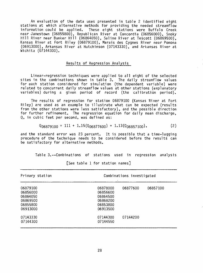
An evaluation of the data uses presented in table 2 identified eight stations at which alternative methods for providing the needed streamflow information could be applied. These eight stations were Buffalo Creek near Jamestown (06855800), Republican River at Concordia (06856000), Smoky Hill River near Bunker Hill (06864050), Saline River at Tescott (06869500), Kansas River at Fort Riley (06879100), Marais des Cygnes River near Pomona (06913000), Arkansas River at Hutchinson (07143330), and Arkansas River at Wichita (07144300).
Results of Regression Analysis
Linear-regression techniques were applied to all eight of the selected sites in the combinations shown in table 3. The daily streamflow values for each station considered for simulation (the dependent variable) were related to concurrent daily streamflow values at other stations (explanatory variables) during a given period of record (the calibration period).
The results of regression for station 06879100 (Kansas 'River at Fort Riley) are used as an example to illustrate what can be expected (results from the other stations were less satisfactory), and the possible direction for further refinement. The regression equation for daily mean discharge, Q, in cubic feet per second, was defined as:
Q06879100 = 1 - 15 (Q06877600) + 1 - 13 (Q06857100) » (2)
and the standard error was 23 percent, procedure of the technique needs to be be satisfactory for alternative methods.
It is possible that a time-lagging considered before the results can
Table 3. Combinations of stations used in regression analysis
[See table 1 for station names]
Primary station Combinations investigated
068791000685600006864050068695000685580006913000
0714333007144300
06878000 068776000685660006864500068682000685380006913500
07144300 0714420007144550
06857100
28

As a result of this preliminary evaluation by regression analysis, it may be beneficial to pursue the application of streamflow-routing, regression methods, and possibly other alternative methods at a later date to determine if the simulated data are sufficiently accurate for the intended data use in lieu of operating a complete-record gaging station. However, none of the stations investigated can presently be simulated with sufficient accuracy from data at other sites.
COST-EFFECTIVE RESOURCE ALLOCATION
Kalman Filtering for Cost-Effective
Resource Allocation (K-CERA)
In a study of the cost effectiveness of a network of gaging stations operated to determine water consumption in the Lower Colorado River Basin, a set of techniques called Kalman filtering for cost-effective resource allocation (K-CERA) was developed (Moss and Gilroy, 1980). Because of the water-balance nature of that study, the measure of effectiveness of the stream-gaging network was chosen to be the minimization of the sum of variances of errors of estimate of annual mean discharges at each site in the network. This measure of effectiveness tends to concentrate stream- gaging resources on the larger, less stable streams where potential errors are greatest. While such a tendency is appropriate for a water-balance network, in the broader context of the multitude of uses of the streamflow data collected in the Survey's streamflow-information program, this tendency causes undue concentration on larger streams. Therefore, the original version of K-CERA was extended to include as optional measures of effective ness the sums of the variances of errors of estimate of the following streamflow variables: annual mean discharge, in cubic feet per second, or average instantaneous discharge, as a percentage. The use of percentage errors does not unduly weight activities at large streams to the detriment of records on small streams. In addition, the instantaneous discharge is the basic variable from which all other streamflow data are derived. For these reasons, this study used the K-CERA techniques with the sums of the variances of the percentage errors of the instantaneous discharges at all complete-record gaging stations as the measure of the effectiveness of the data-collection activity.
The original version of K-CERA also did not account for error con tributed by missing stage or other correlative data that are used to compute streamflow data. The probabilities of missing correlative data increase as the period between service visits to a gaging station increases. A proce dure for dealing with the missing record was developed and incorporated into this study.
Brief descriptions of the mathematical program used to optimize cost effectiveness of the data-collection activity and of the application of Kalman filtering (Gelb, 1974) to the determination of the accuracy of a stream-gaging record are presented below. For more detail on either the theory or the applications of K-CERA, see Moss and Gilroy (1980), Gilroy and Moss (1981), and Fontaine and others (1984).
29

Description of Mathematical Program
The mathematical program used in K-CERA, called "The Traveling Hydro- grapher," attempts to allocate among gaging stations a predefined budget for the collection of streamflow data in such a manner that operation is the most cost effective possible. The measure of effectiveness was discussed in the preceding section. The set of decisions available to the manager is the frequency of use (number of times per year) of each of a number of routes that may be used to service the gaging stations and to make discharge meas urements. The range of options within the program is from zero usage to daily usage for each route. A route is defined as a set of one or more gaging stations and the least-cost travel that takes the hydrographer from his base of operations to each of the stations and back to base. A route will have associated with it an average cost of travel and an average cost of servicing each gaging station visited along the way. The first step in this part of the program is to define the set of practical routes. This set of routes frequently will contain the path to an individual gaging station with that station as the lone stop and return to base so that the individual needs of a gaging station can be considered in isolation from the other stations.
Another step in this part of the program is the determination of any special requirements for visits to each of the stations for such things as necessary periodic maintenance, rejuvenation of recording equipment, or re quired periodic sampling of water-quality data. Such special requirements are considered to be inviolable constraints in terms of the minimum number of visits to each station.
The final step is to use all of the above to determine the number of times, N-J, that the ith route for i = 1, 2, ..., NR, where NR is the number of practical routes, is used during a year such that (1) the budget for the network is not exceeded, (2) the minimum number of visits to each station is made, and (3) the total uncertainty in the network is minimized. Figure 3 represents this step in the form of a mathematical program. Figure 4 presents a tabular layout of the problem. Each of the NR routes is repre sented by a row of the table, and each of the stations is represented by a column. The zero-one matrix ( w ij) defines the routes in terms of the stations that comprise it. A value of 1 in row i and column j indicates that gaging station j will be visited on route i; a value of 0 indicates that it will not. The unit travel costs (3j) are the per-trip costs of the hydrographer 's travel time and any related per diem and operation, mainte nance, and rental costs of vehicles. The sum of the products of 3j and NT for i = 1, 2, ..., NR is the total travel cost associated with the set of decisions N = (Nj, N2» ..., NNR ).
The unit-visit cost (aj ) is comprised of the average service and main tenance costs incurred on a visit to the station plus the average cost of making a discharge measurement. The set of minimum visit constraints is de noted by the row AJ, j = 1, 2,..., MG, where MG is the number of stations. The row of integers n j , j = 1, 2, ..., MG, specifies the number of visits to each station. Mj is the sum of the products of w-jj and N-J for all i and must equal or exceed Aj for all j if N is to be a feasible solution to the decision problem.
30

MG Minimize V = Z <J>. (Af.),N_ 3'ml 3 J
whereV E total uncertainty in the network;
N_ E vector of annual number times each route was used;
MG E number of gages in the network;
M. E annual number of visits to station j; and
(j) . E function relating number of visits to uncertainty at station j-
Such that
Budget _> T Etotal cost of operating the network
MG NR T = F + Z a.M. + Z &.N. ,
whereF E fixed cost; c
a. E unit cost of visit to station j ;
NR E number of practical routes chosen;
3- E travel cost for route i; and
N. E annual number times route i is used (an element of //);
and such that
M. > \. , 3 0
where \ . =. minimum number of annual visits to station j .
Figure 3. Mathematical-programing form for optimization of hydrographerrouting.
The total cost expended at the stations is equal to the sum of the products of dj and Mi for all j. The costs of record computation, docu mentation, and publication are assumed to be influenced negligibly by the number of visits to the station and are included along with overhead in the fixed cost of operating the network. The total cost of operating the net work equals the sum of the travel costs, the onsite costs, and the fixed cost, and must be less than or equal to the available budget.
The total uncertainty in the estimates of discharges at the MG stations is determined by summing the uncertainty functions (4>-j) evaluated at the value of MJ from the row above it, for j = 1, 2, ...,
31

Route
1
2
3
4
z
NR
UnitVisit CostMinimum VisitsVisits
Uncertain
Gage 1 2 3 4 . j' . MG
1 0 0 0 ... 0 1 1 0 0 ... 0
1 0 0 0 ... 0
0 1 0 0 ... 0
i] '
0 0 0 0 ... 1
<X| (%2 #3 #4 . Oi- . <3jv)G
A\ A,2 AS A.4 . Aj . AMG
Af-i Af2 ^3 ^4 ^/' MMGv
' ty01 02 03 04 0/ 0MG
Unit Travel Cost
02
03
A-
0NR
vAt-sit Cost/ I
*?N
Uses
#1
^.'
^R
* ^^^ Travel
Cost9 7,j^Total _ /; Cost ̂
Budget
Minimum,
Figure 4.--Tabular form for optimization of hydrographer routing.
As pointed out in Moss and Gilroy (1980), the steepest-descent search used to solve this mathematical program does not guarantee a true optimum solution. However, the locally optimum set of values for _N obtained with this technique specify an efficient strategy for operating the network, which may be the true optimum strategy. The true optimum cannot be guaran teed without testing all undominated, feasible strategies.
Description of Uncertainty Functions
As noted earlier, uncertainty in streamflow records is measured in this study as the average relative variance of estimation of instantaneous discharges. The accuracy of a streamflow estimate depends on how that esti mate was obtained. Three situations were considered in this study: (1)
32

streamflow was estimated from measured discharge and correlative data using a stage-discharge relation (rating curve); (2) the streamflow record was reconstructed using secondary data at nearby stations because primary cor relative data were missing; and (3) primary and secondary data were unavail able for estimating streamflow. The variances of the errors of the estimates of flow that would be employed in each situation were weighted by the frac tion of time each situation was expected to occur. Thus, the average relative variance would be
V = ef Vf + £rVp + ee Ve , (3)
with
1 = ef + ep + ee»
where "V is the average relative variance of the errors of streamflow esti mates;
ef is the fraction of time that the primary recorders are functioning;
Vf is the relative variance of the errors of flow estimates from pri mary recorders;
e r is the fraction of time that secondary data are available to recon struct streamflow records given that the primary data are miss ing;
V r is the relative variance of the errors of estimate of flows recon structed from secondary data;
e e is the fraction of time that primary and secondary data are not available to compute streamflow records; and
Ve is the relative error variance of the third station.
The fractions of time that each source of error is relevant are func tions of the frequencies at which the recording equipment is serviced.
The time (T) since the last service visit until failure of the recorder or recorders at the primary site was assumed to have a negative-exponential probability distribution truncated at the next service time; the distribu tion's probability density function is
f(i) = kd-kT/(i-e- k S), (4)
where k is the failure rate in units of (day)' 1 ;e is the base of natural logarithms; ands is the interval between visits to the site, in days.
It was assumed that, if a recorder failed it continued to malfunction until the next service visit. As a result,
ef = (l-e- ks )/(ks) (5)
(Fontaine and others, 1984, equation 21).
33

The fraction of time (e e ) that no records existed at either the primary or secondary sites also could be derived assuming that the time between failures at both sites was independent and had negative-exponential distri butions with the same rate constant. It then follows that
£ e = 1 - [2(l-e-ks ) + 0.5(l-e-2ks )]/(ks)
(Fontaine and others, 1984, equations 23 and 25).
Finally, the fraction of time (e r ) that records were reconstructed based on data from a secondary site was determined by the equation
£ - 1 £_ £r ~ x " f " e
= [(l-e-ks ) + 0.5(l-e-2ks )]/(ks). (6)
The relative variance (Vf) of the error derived from primary-record computation was determined by analyzing a time series of residuals that were the differences between the logarithms of measured discharge and the rating- curve discharge. The rating-curve discharge was determined from a relation ship between discharge and some correlative data, such as water-surface elevation at the gaging station. The measured discharge was the discharge determined by onsite observations of depths, widths, and velocities. Let qj(t) be the true instantaneous discharge at time t, and let qR(t) be the value that would be estimated using the rating curve. Then, the equation
x(t) = In q T (t) - In q R (t) = In Eq R (t)] (7)
is the instantaneous difference between the logarithms of the true discharge and the rating-curve discharge.
In computing estimates of streamflow, the rating curve may be continu ally adjusted on the basis of periodic measurements of discharge. This ad justment process resulted in an estimate, qc (t), that was a better estimate of the stream's discharge at time t. The difference between the variable x(t), which is defined as
x(t) = In qc (t) - In qR (t), (8)
and x(t) was the error in the streamflow record at time t. The variance of this difference over time was the desired estimate of Vf.
Unfortunately, the true instantaneous discharge, qj(t), could not be determined, and thus x(t) and the difference, x(t) - x(t), could not be de termined as well. However, the statistical properties of x(t) - x(t), particularly its variance, could be inferred from the available discharge measurements. Let the observed residuals of measured discharge from the rating curve be z(t) so that
z(t) = x(t) + v(t) = In qm (t) - In q R (t), (9)
34

where v(t) is the measurement of error; and
In q m (t) is the logarithm of the measured discharge equal to In qj(t) plus v(t).
In the Kalman-filtering analysis, the z(t) times series was analyzed to determine three site-specific parameters. The Kalman-filter technique used in this study assumes that the time residuals x(t) arise from a continu ous first-order Markovian process that has a Gaussian (normal) probability distribution with zero mean and variance (subsequently referred to as pro cess variance) equal to p. Another important parameter is 3, the reciprocal of the correlation time of the Markovian process giving rise to x(t); the correlation between x(ti) and x(t2) is exp[-3 |ti-t2J]. Fontaine and others (1984) also define q, the constant value of the spectral density function of the white noise, which drives the Gauss-Markov x-process. The parameters p, 3, and q, are related by
Var[x(t)] = p = q/(23). (10)
The variance of the observed residuals z(t) is
Var[z(t)] = p + r, (11)
where r is the variance of the measurement error v(t). The three para meters p, 3, and r are computed by analyzing the statistical properties of the z(t) time series. These three site-specific parameters are needed to define this component of the uncertainty relationship. The Kalman-filter technique utilizes these three parameters to determine the average relative variance of the errors of estimate of discharges as a function of the number of discharge measurements per year (Moss and Gilroy, 1980).
If the recorder at the primary site failed and there were no concurrent data at other sites that could be used to reconstruct the missing record at the primary site, there were at least two ways of estimating discharges at the primary site. A recession curve could be applied from the time of recorder stoppage until the gage was once again functioning, or the expected value of discharge for the period of missing data could be used as an esti mate. The expected-value approach was used in this study to estimate Ve , the relative error variance during periods of no concurrent data at nearby stations. If the expected value was used to estimate discharge, the value that was used should have been the expected value of discharge at the time of year of the missing record because of the seasonality of the streamflow processes. The variance of streamflow, which also is a seasonally varying parameter, is an estimate of the error variance that results from using the expected value as an estimate. Thus, the coefficient of variation squared [(Cv ) ] is an estimate of the required relative error variance Ve . Because C v varies seasonally and the times of failures cannot be antici pated, a seasonally averaged value of Cv was used:
1 365 ,al\2 1/2(12)
35

where a-
y.j
is the standard deviation of daily discharges for the i th day of the year;
is the expected value of discharge on the i**" day of the year;. O
and (C") is used as an estimate of V e .
The variance (V r ) of the relative error during periods of reconstructed streamflow records was estimated on the basis of correlation between records at the primary site and records from other nearby gaged sites. The corre lation coefficient (pc ) between the streamflows with seasonal trends removed at the site of interest and detrended streamflows at the other sites is a measure of the "goodness" of their linear relationship. The fraction of the variance of streamflow at the primary site that is explained by data from other sites is equal to Pc . Thus, the relative error variance of flow estimates at the primary site obtained from secondary information will be
V P = (1- (13)
Because errors in streamflow estimates arise from three different sources with widely varying precisions, the resultant distribution of those errors may differ significantly from a normal or log-normal dis tribution. This lack of normality causes difficulty in interpretation of the resulting average estimation variance. When primary and secondary data are unavailable, the relative error variance^ V e may be very large. This could yield correspondingly large values of V in equation (3) even if the probability that primary and secondary information are not available, e e , is quite small.
A new parameter, the equivalent Gaussian spread (EGS), is introduced here to assist in interpreting the results of the analyses. If it is assumed that the various errors arising from the three situations repre sented in equation (3) are log-normally distributed, the value of EGS was determined by the probability statement that
Probability [e"EGS <_ (qc (t) /qT (t)) 1 e +EGS] = 0.683 (14)
Thus, if the residuals In q c (t) - q-j-(t) were normally distributed, (EGS) 2 would be their variance. Here EGS is reported in units of percent because EGS is defined so that nearly two-thirds of the errors in instantaneous streamflow data will be within plus or minus EGS percent of the reported values.
Application of K-CERA in Kansas
In the 1983 operation of routine visits to data-collection sites in Kansas, there were 140 complete-record stations and 137 other stations (reservoir stage, crest-stage, precipitation, and flood rating) that were considered or accounted for in this evaluation. As a result of the first two parts of this evaluation, it has been found that the 140 complete-record stations operated during 1983 in Kansas were needed to meet the data-use requirements. The station records were examined and screened for those
36

stations that were acceptable for further analysis. However, uncertainty functions could not be defined for those stations that were typically ephemeral and had a large number of zero-flow days, or those that did not have sufficient number of discharge measurements for rating definition (period of record at present site was short, or rating not adequately defined due to backwater conditions); these stations were considered in a different category for the application of the "Traveling Hydrographer Program" that will follow. Ninety-one stations were selected for the K-CERA analysis with results that are described below.
Definition of Missing-Record Probabilities
As was described earlier, the statistical characteristics of missing stage or other correlative data for computation of streamflow records can be defined by a single parameter, the value of k in the truncated negative- exponential probability distribution of times to failure of the equipment. In the representation of f(x) as given in equation 4, the average time to failure is 1/k. The value of 1/k will vary from station to station depending on the type of equipment at the station and on its exposure to natural elements and vandalism. The value of 1/k can be changed by advances in the technology of data collection and recording. For the value of 1/k in Kansas, it was estimated that a gage could be expected to malfunction 5.5 percent of the time (D. L. Lacock, U.S. Geological Survery, oral commun., 1983). There was no reason to distinguish between gages on the basis of their exposure or equipment, so a 5.5-percent lost record and a 6-week visit frequency were used to determine a value of 1/k for 305 days, which was used to determine e f, e e , and e r for each of the 91 gaging stations as a function of the individual frequencies of visit.
Definition of Cross-Correlation Coefficient and
Coefficient of Variation
To compute the values of Ve and V r of the needed uncertainty func tions, daily streamflow records for each of the 91 stations for the last 30 years or the part of the last 30 years for which daily streamflow values are stored in WATSTORE (Hutchison, 1975) were retrieved. For each of the Stations that had 3 or more complete water years of data, the value of C v was computed.
Many different sources of information are normally used to recon struct periods of missing record. These sources include, but are not limited to, recorded ranges in stage (for graphic recorders with clock stoppage), known discharges on adjacent days, recession analysis, observers' staff-gage readings, weather records, high-water-mark elevations, and compar isons with nearby stations. However, most of these techniques are unique to a given station or to a specific period of lost record. Using all the tools available, short periods (several days) of lost record usually can be reconstructed quite accurately. Even longer periods (more than a month) of missing record can be reconstructed with reasonable accuracy if observers'
37

readings are available. If, however, none of these tools are available, long reconstructions can be subject to large errors.
The study could not reasonably quantify the uncertainty that is asso ciated with all the possible methods of reconstructing missing record at the individual stations. Therefore, this evaluation assumed that missing record would be reconstructed based on historical discharges for that season or from correlation with data from another gaging station. The fraction of time each approach was used was dependent on the frequency at which the gage was serviced. Both of the approaches used in this evaluation undoubtedly overstated the uncertainty of reconstructing a short period of missing record; the stated uncertainty may be reasonable for long periods of missing record.
Historically, operating procedures have caused most periods of missing record to be measured in days rather than months. Given the small cross- correlations and the relatively large variability of flow usually occurring in Kansas, this evaluation seemed to significantly overstate the uncertainty associated with missing record. Therefore, in Kansas, a value of 0.95 was used for the cross-correlation coefficient. In reconstructing records, the cross-correlation coefficient, therefore, was used as a surrogate for the knowledge of basin response that remains unquantified in the present study. This assumption is believed to be reasonable for short periods of missing record; it probably caused the uncertainty to be understated for long periods of lost record.
The value of C~v for each station is summarized in table 4. In the table, there are six stations that are flagged for a computed coefficient for the process variance that is larger than acceptable. The probable reason could be that the rating from which the residuals were determined may not be described properly with a single continuous function. This meant that the error was overestimated. The stations were kept in the analysis, but the uncertainty functions were given zero weight. The con sequences of this decision are discussed later with the K-CERA results.
Kalman-Filtering Definition of Variance
The determination of the variance Vf for each of the 91 gaging stations required three distinct steps: (1) Long-term rating analysis and computa tion of residuals of measured discharges from the long-term rating, (2) time-series analysis of the residuals to determine the input parameters for the Kalman-filtering process, and (3) computation of the error variance (Vf) as a function of the time-series parameters, the discharge-measurement- error variance, and the frequency of discharge measurement.
In the evaluation of the 1983 Kansas program, definition of long-term rating functions was complicated by the fact that most gaging stations in Kansas have the dual seasonal characteristic of a summer or open-water period and a winter or backwater period. As a result of this characteristic, a single-rating function to define the entire year was not feasible. The winter discharge at a given station is typically determined from possible combinations of: (1) Data from the station, measured stage, and the dis charge corresponding to the measured stage determined from the open-water
38

Table 4.--Summary of autocovariance analysis and coefficient of variation
Station number
0681400006853500068560000685660006857100
0686000006861000068627000686350006864050
0686450006865500068665000686700006868200
0686950006870200068725000687400006875900
0687644006876700068769000687760006878000
0687910006884200068844000688550006887000
0688750006888500068890000688914006889160
0688920006889500068901000689100006892000
RHOl/
0.988.9916.988.9742.985
.981
.926
.975
.992
.974
.987
.992
.985
.997
.996
.999
.999
.996
.995
.990
.985
.991
.993
.987
.997
.989
.994
.419
.978
.983
.972
.984
.989
.951
.989
.992
.993
.991
.992
.999
Process variance
(log base e)-
1/0.244.0613.0484.0174.133
.1321/.224
.0392
.0987
.0639
.109
.106
.0593
.074
.0997
.0428
.0079
.0763
.0942
.00124
.0734
.087
.0524
.0226
.0445
.0268
.1225
.0293
.0883
.113
.011
.0620
.03952/.219
.142
.158
.0902
.1035
.0125-2/.221
Coefficient of variation
/ C L v
2.5831.3811.3471.4441.360
2.5462.4191.2922.0641.982
1.9411.7851.5831.6762.465
2.0871.7481.9291.9892.169
1.0892.4861.9021.5882.328
1.4262.3131.5622.5971.595
1.3052.0061.2802.4742.337
2.2302.4232.0681.2992.459
Number of
observations
9592877890
102119939670
997685110106
10434949640
3496
10611294
87931089698
90117189112116
125118116104108
39

Table 4.--Summary of autocovariance analysis and coefficient of variation- Continued
Station number
0689235006910800069115000691190006912500
0681300006913500069140000691660006917000
0691738007137500071380000714000007141300
0714230007142575071426200714330007143330
0714366507144200071443000714455007144780
0714479507145200071455000714570007146500
0714707007147800071490000715150007157500
RHOl/
0.986.996.978.406.994
.969
.938
.923
.953
.982
.936
.992
.985
.996
.992
.998
.991
.991
.973
.993
.994
.995
.987
.995
.991
.990
.982
.989
.994
.993
.989
.987
.988
.994
.961
Process variance
(log base e)^/
0.0142.0836.0700.0801.0726
.0291
.0091
.1007
.0304
.0646
.0906
.121
.165
.0839
.165
.157
.111
.186
.083
.0926
.0709
.0832
.0468
.0837
.1437
.0947
.074
.0582/.297
.0795
.0588
.0938
.081
.0945
.1004
Coefficient of variation
c v
1.3061.9792.9202.4102.444
1.6722.1912.9341.9232.674
1.9711.3241.3151.5691.835
1.3781.1371.4892.2081.363
1.8972.3921.6111.2971.472
2.3861.3301.5832.1521.407
2.2152.2851.5041.6352.042
Number of
observations
165108121103120
122122129100115
12928821712292
1088098103107
967110396193
1129894108108
1091071015499
40

Table 4. Summary of autocovariance analysis and coefficient of variation- Continued
Station number RHOl/
Process variance
(log base e)
Coefficient of vaiation
Numberof
observations
0716600007166500071685000716950007170060
0717050007172000071795000717973007179795
0718040007180500071822500718251007183000
07183500
0.999.941.975.916.987
.959
.982
.986
.987
.984
.982
.989
.991
.982
.983
.991
0.0961.0818.0651.0256
2/.317
.0427
.106
.0814 '.0877 .0924
.048
.102
.0284
.0717
.0155
.0443
2.2252.1222.2112.1372.212
2.0492.5442.551.9142.204
1.8612.2181.6821.6651.789
1.792
223173204188222
19618610010054
1029497113110
114
1 One-day autocorrelation coefficient.2 The value of the process variance indicates that the rating is not
adequately defined.
rating; (2) climatological data obtained from the National Weather Service sites closest to the gaging station, including the maximum and minimum temperature for the given day and the total precipitation that occurred as rain for the day and the previous day; and (3) the daily mean discharge, based on the open-water rating curve, for stations that are proximate or physiographically similar or both to the stations being considered. The winter period is not long enough and the effects of ice are too variable to define a winter rating, and there can be alternate freezing and thawing during the winter period. Therefore, only the open-water period was con sidered for this evaluation. The stations in the northern part of the State have a longer winter period than those in the southern part, so an average open-water period of 305 days was used for the entire State (D. L. Lacock, U.S. Geological Survey, oral commun., 1983).
The time series of residuals for open-water measurements is used to compute sample estimates of q and 3, two of the three parameters required to compute Vf, by determining a best-fit autocovariance function to the time series of residuals. Measurement variance, the third parameter, is determined from an assumed constant percentage standard error. For the Kansas program, all open-water measurements were assumed to have a measure ment error of 3.5 percent.
41

70 1 1 1 1 1 1
STATION
06864500
UJo ocUJ Q.
<r o oc oc
o oc
CO
06887500
10 15 20 25
NUMBER OF VISITS AND MEASUREMENTS
35
Figure 5. Typical uncertainty functions for instantaneous discharge.
The autocovariance parameters and data from the definition of missing- record probabilities, summarized in table 4, are used jointly to define un certainty functions for each gaging station. The uncertainty functions give the relationship of total error variance to the number of visits and discharge measurements. Typical examples of the uncertainty functions are given in figure 5. These functions are based on the assumption that a measurement was made during each visit to the station. Some stations are not measured every visit due to conditions such as zero flow. Therefore, the probability of making a discharge measurement during any visit (less than 1.0 and varies according to each station) is part of the analysis.
In Kansas, feasible routes to service the data-collection sites were determined after consultation with personnel responsible for the data collection and after review of the uncertainty functions. The 277 sites considered included 91 complete-record stations with the determined un certainty functions, 49 complete-record stations without uncertainty func-
42

tions that were also part of the 1983 program, and the other 137 partial- record stations that were visited on a routine schedule. In summary, 65 routes were selected to service all the stations in Kansas. These routes included possible combinations that described the 1983 operating practice, alternatives that were under consideration as future possibilities, routes that visited certain key individual stations, and combinations that included proximate stations where the levels of uncertainty indicated more frequent visits might be useful. In addition, minimum visits were considered, as well as special scheduled requirements, such as water-quality sampling, monthly requirements for the National Water Conditions Report, and crest- stage gage inspections.
The costs associated with the practical routes were determined. Fixed costs to operate a station typically included equipment rental, batteries, electricity, data processing and storage, computer charges, maintenance and miscellaneous supplies, and analysis and supervisory charges. For Kansas, average values were applied to each station in the 1983 program for all the above categories, afld additional costs for telemetry maintenance and spe cial-measurement requirements were added, where applicable. Costs of the travel for the winter-period visits were added to the fixed costs of each station.
Visit costs were those associated with paying the hydrographer for the time actually spent at a station servicing the equipment and making a discharge measurement. These costs varied from station to station and were a function of the difficulty and time required to make the discharge measurement. Average visit times were calculated for each station based on an analysis of discharge-measurement data available. This time then was multiplied by the average hourly salary of hydrographers in the Kansas office of the Survey to determine total visit costs.
Route costs included the vehicle cost associated with driving the num ber of miles it takes to cover the route, the cost of the hydrographer's time while in transit, and any per diem associated with the time it takes to complete the trip.
K-CERA Results
The "Traveling Hydrographer Program" utilizes the uncertainty functions along with the appropriate cost data and route definitions to compute the most cost-effective way of operating the stream-gaging program. In this application, the first step was to simulate the 1983 practice and deter mine the total uncertainty associated with it. To accomplish this, the number of visits being made to each station and the specific routes that were being used to make these visits were fixed. In Kansas, 1983 practice indicated that station visits were being made on a 6-week basis, which is nine visits a year. One visit a year was allowed for the winter season; therefore, the 1983 practice for the open-water analysis was eight visits per year. The resulting average error of estimate for the 1983 practice in Kansas was plotted as 20.8 percent in figure 6. The solid line in figure 6 represents the minimum level of average uncertainty that can be ob tained for a given budget with the existing instrumentation and technology. The line was defined by several runs of the "Traveling Hydrographer Program"
43

AV
ER
AG
E
ST
AN
DA
RD
E
RR
OR
, IN
P
ER
CE
NT
c+ c
o S
r+
IT r
> Q>
-"
O
IT
r+
O
CO
fD
fD
13fD
Q
. -j
COC
I
CO
<_Q
-b
r+
fD
C
Oa>
CD
-
S
-"<
/>
O
O
c+
<" IT _
j o
_
fD
-o
3
fD
O
<
j. fD
C
<]>
,r+
fD
3 i
"<
0
00
fD
c-t-
-3
CO5T
* X
I -.
13 O
- w
COc co
T
I »-
t rt
r+
fD
O
IT IT
CU
O-
-J
fD
fD
I
IT-Q
£U
-"
O
O
fD
-
fD
-"
fD
C '<
CO
c+
CO
-jr+
- C
fD
lSC
IT
-1'
fD3"
Q-"
O
fD
r+
~J
O
r+
C3
<
C
UQ
-fD
I
O-O
- -j
fD
S
-"
-J-
_O
O-
O
fD
-"
c+ r+
CO
'
-j-v
. <-
+O
n-
co
coQ
- -
fD
rt
-*
O
ZT
c+
O^fD
co
^^o-
CQ
O
-i.
n)
CU to
°-
-J
_j. C
UCO r+
-
Q.
CXJ
_i.
Q-C
Q
CO
-t,
fD
fD
fD
fD
fD
-J
Q.
fD
CO O-^
fD
5.
<^ tQ
Q
m
2.
<"*
o-S
0fD
Q
.
fD
CO O 13 r+ IT
fD O -o fD -J
CXJ
r+
O 13
CO o c+ IT
fD O-
CQ
fD
CQ CT
i
fD -J
CXJ
CQ
fD cu zs
O
. cu
-j
Q-
fD CO
CX
JC
O
fD

as the minimum requirement, as well as for reservoirs.
The results in figure 6 and table 5 summarize the K-CERA analysis and are predicated on the basis that a discharge measurement was made at the estimated probability of making the measurement of each respective station, each time that a station was visited.
The six stations that were footnoted in table 4 were given a weight of zero for the "Traveling Hydrographer Program." Although an estimate of error was computed, based on the 1983 visitation schedule, this did not contribute to the total variance of error. Because of this special treatment of the six stations, the total variance of error was based on 85 of 140 stations.
It should be emphasized that figure 6 and table 5 are based on various assumptions (stated previously) concerning both the time series of shifts to the stage-discharge relationship and the methods of record construction. Where a choice of assumptions was available, the assumption that would not underestimate the magnitude of the error variances was chosen.
It can be seem that the 1983 schedule results in an average standard error of estimate of instantaneous discharge of 20.8 percent. This schedule required a budget of $793,780 to operate the 140 continuous-record stations and the 137 other sites in the stream-gaging program. It should be noted that the error of estimate is based on only 85 of the 140 complete-record stations. The range in standard errors was from a minimum of 9.6 percent for station 06892350 to a maximum of 36.5 percent for station 06914000.
It would be possible to decrease the average standard error by altering the travel routes and the measurement frequency while maintaining the same budget of $793,780. In this case, the average standard error would decrease from 20.8 to 18.9 percent. Extremes of standard errors for individual sites would be 9.4 and 31.0 percent for stations 06892350 and 06914000, respectively.
A minimum budget of $760,000 is required to operate the 1983 stream- gaging program; a budget of less than this would not permit proper service and maintenance of the gages and recorders. Stations would have to be eliminated from the program if the budget were less than this minimum. At the minimum budget, the average standard error would be 24.9 percent. The minimum standard error of 9.4 percent would occur at station 06892350, whereas the maximum standard error of 39.8 percent would occur at station 06914000.
The maximum budget analyzed was $1,191,000, which resulted in an aver age standard error of estimate of 8.6 percent. Thus, a budget almost one-half again as large, in conjunction with schedule change would almost halve the average standard error that would result fom the 1983 schedule and budget. For the $1,191,000 budget, the extremes of standard error were 4.6 percent for station 06891000 and 14.5 percent for station 06914000. Thus, it is apparent that significant improvements in accuracy of streamflow records can be obtained if larger budgets become available.
45

Table 5. Selected results of K-CERA analysis
Station number
Average per station \J
06853500
06856000
06856600
06857100
06860000
06862700
06863500
06864050
06864500
06865500
Standard error in instantaneous discharge, in percent [Equivalent Gaussian spread]
(Number of visits per year to site)
Current operation
20.8
10.2 [3.1] (8)
13.0 [9.6] (8)
12.8 [8.3](8)
17.1 [15.2]
(8)
25.3 [18.2]
(8)
14.5 [12.1]
(8)
18.5 [11.3]
(8)
20.2 [15.8]
(8)
20.0 [15.1]
(8)
16.1 [11.5]
(8)
Bi 760
24.9
12.8 [4.0] (5)
16.2 [12.3]
(5)
15.6 [10.2]
(5)
21.1 [19.2]
(5)
25.3 [18.2]
(8)
16.3 [13.8]
(6)
21.2 [13.3]
(6)
22.9 [17.9]
(6)
24.8 [19.3]
(5)
20.1 [14.9]
(5)
jdget, in tl 779
20.8
12.8 [4.0] (5)
16.2 [12.3]
(5)
15.6 [10.2] (5)
21.1 [19.2]
(5)
20.9 [14.8] (12)
13.1 [10.9] (10)
16.7 [10.0] (10)
18.3 [14.2] (10)
20.0 [15.0]
(8)
20.1 [14.9]
(5)
lousands of 793.8
18.9
11.7 [3.6] (6)
14.9 [11.2]
(6)
14.5 [9.4] (6)
19.5 [17.6]
(6)
19.4 [13.6] (14)
13.1 [10.9] (10)
16.7 [10.0] (10)
18.3 [14.2] (10)
20.0 [15.0] (8)
17.1 [12.4] (7)
1982 doll a 834
15.6
9.2 [2.8] (10)
11.7 [8.6] (10)
11.5 [7.4] (10)
15.4 [13.5] (10)
18.8 [13.2] (15)
11.2 [9.2] (14)
14.1 [8.3] (14)
15.7 [12.0] (14)
18.0 [13.3] (10)
13.8 [9.7] (ID
rs 1191
8.6
5.2 [1.9] (33)
6.6 [4.6] (33)
6.5 [4.1] (33)
8.6 [7.3] (33)
8.9 [6.0]
. (68)
5.9 [4.7] (53)
7.4 [4.3] (53)
8 0 .£
[6.1] (53)
8.9 [6.3] (42)
8.1 [5.5] (34)
1 Square root of seasonally averaged station variance.
46

Table 5. Selected results of K-CERA analysis Continued
Station number
06866500
06867000
06868200
06869500
06870200
06872500
06874000
06875900
06876440
06876700
Standard error in instantaneous discharge, in percent [Equivalent Gaussian spread]
(Number of visits per year to site)
Current operation
15.3 [11.8]
(8)
12.8 [5.5] (10)
20.6 [8.1] (8)
15.8 [3.0] (8)
11.1 [1.3] (8)
15.1 [7.0] (8)
16.9 [8.8] (8)
10.6 [2.4] (8)
14.0 [12.9]
(8)
21.5 [11.9]
(8)
Bi 760
18.9 [14.9]
(5)
12.8 [5.5] (10)
25.7 [10.8]
(5)
19.7 [3.8] (5)
13.9 [1.7] (5)
18.9 [9.3] (5)
21.0 [11.5]
(5)
13.3 [2.9] (5)
17.2 [16.2]
(5)
26.8 [15.6]
(5)
jdget, in tt 779
18.9 [14.9]
(5)
12.2[5.2](11)
19.5 [7.7] (9)
18.1 [3.4] (6)
13.9 [1.7] (5)
15.1 [7.0] (8)
16.8 [8.8] (8)
12.2 [2.7] (6)
17.2 [16.2]
(5)
24.6 [14.0]
(6)
lousands of 793.8
16.2 [12.6] (7)
12.2 [5.2] (ID
19.5 [7.7] (9)
15.0 [2.8] (9)
11.8 [1.4] (7)
15.1 [7.0] (8)
16.9 [8.8] (8)
10.0 [2.3] (9)
14.9 [13.8] (7)
20.0 [11.2] (9)
1982 dollar 834
13.1 [10.0](ID
10.9 [4.6] (14)
18.5 [7.2] (10)
12.1 [2.2] (14)
9.5 [1.2] (ID
13.6 [6.2] (10)
15.2 [7.8] (10)
8.1 [1.9] (14)
12.0 [11.0] (ID
16.4 [8.7] (14)
"S
1191
7.6 [5.6] (34)
5.4 [2.4] (61)
8.5 [3.3] (50)
6.8 [1.4] (45)
5.4 [0.75] (34)
6.8 [3.2] (42)
7.6 [3.8] (42)
4.6 [1.2] (45)
6.9 [6.1] (34)
9.3 [4.8] (45)
47

Table 5. Selected results of K-CERA analysis Continued
Station number
06876900
06877600
06878000
06879100
06884200
06884400
06885500
06887000
06887500
06888500
Standard error in instantaneous discharge, in percent [Equivalent Gaussian spread]
(Number of visits per year to site)
Current operation
16.5 [7.8] (8)
13.9 [7.1] (8)
17.1 [4.8] (8)
12.0 [7.0] (8)
18.7 [9.8] (8)
11.0 [1.2] (10)
25.1 [17.4]
(8)
19.9 [17.3]
(8)
11.2 [6.8] (8)
19.9 [12.8]
(8)
Bi 760
20.5 [10.3]
(5)
17.3 [9.1] (5)
21.4 [6.3] (5)
14.9 [9.0] (5)
23.4 [12.9]
(5)
11.0 [1.2] (10)
30.8 [21.8]
(5)
24.4 [21.7]
(5)
13.7 [8.3] (5)
24.6 [16.4]
(5)
idget, in tr 779
18.8 [9.3] (6)
17.3 [9.1] (5)
19.6 [5.6] (6)
12.8 [7.5] (7)
18.7 [9.8] (8)
11.0 [1.2] (10)
25.1 [17.4] (8)
21.1 [18.5]
(7)
13.7 [8.3] (5)
21.2 [13.7]
(7)
lousands of 793.8
15.6 [7.4]
. (9)
15.9 [8.3] (6)
17.1 [4.8] (8)
12.0 [7.0] (8)
16.8 [8.7] (10)
11.0 [1.2] (10)
22.6 [15.7] (10)
19.9 [17.3] (8)
13.7 [8.3] (5)
18.9 [12.0] (9)
1982 dollar 834
12.6 [5.8] (14)
12.5 [6.3] (10)
13.5 [3.8] (13)
9.5 [5.4] (13)
13.4 [6.8] (16)
9.7 [0.87] (13)
18.1 [12.2] (16)
15.9 [13.5] (13)
13.7 [8.3] (5)
17.2 [10.7](ID
*s 1191
7.1 [3.2] (45)
7.0 [3.4] (33)
7.5 [2.1] (44)
5.2 [3.0] (45)
7.3 [3.7] (56)
5.3 [0.80] (45)
9.8 [6.4] (56)
8.6 [7.0] (45)
7.5 [4.6] (19)
8.7 [5.2] (44)
48
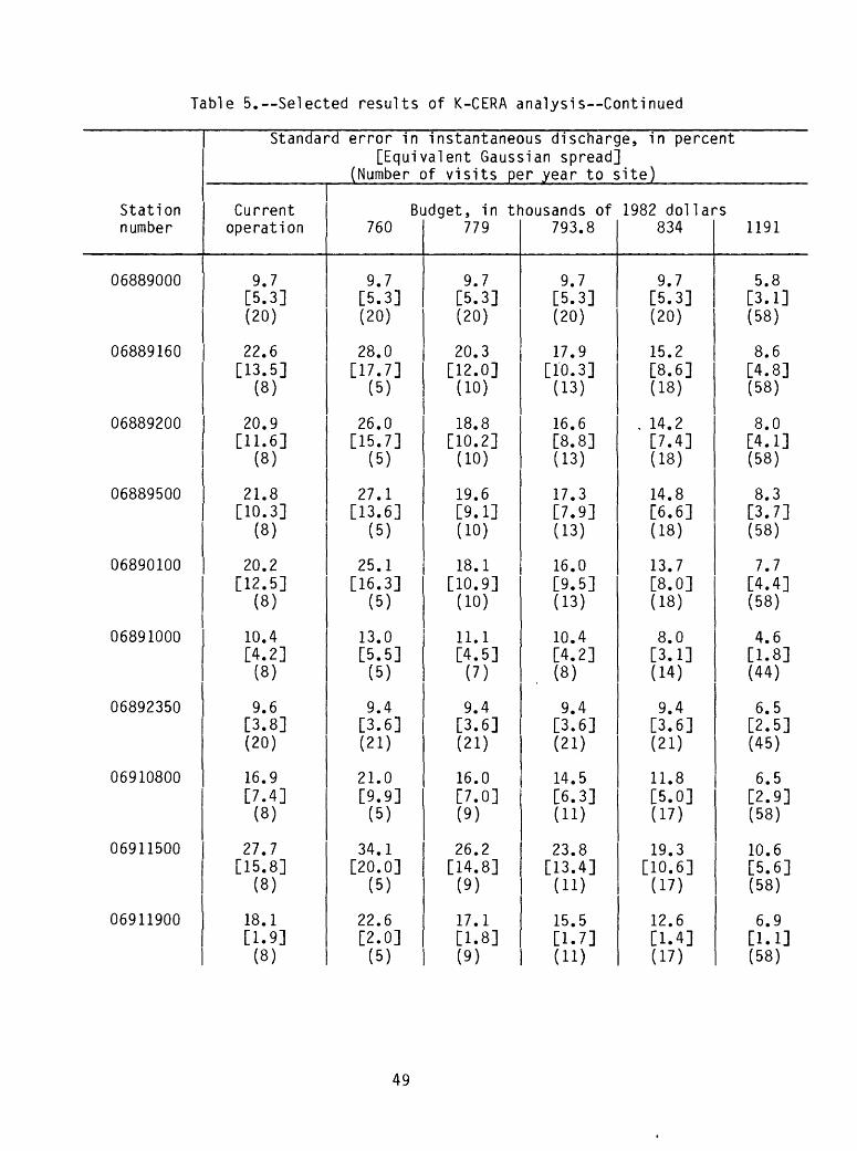
Table 5. Selected results of K-CERA analysis Continued
Station number
06889000
06889160
06889200
06889500
06890100
06891000
06892350
06910800
06911500
06911900
Standard error in instantaneous discharge, in percent [Equivalent Gaussian spread]
(Number of visits per year to site)
Current operation
9.7 [5.3] (20)
22.6 [13.5]
(8)
20.9 [11.6]
(8)
21.8 [10.3]
(8)
20.2 [12.5]
(8)
10.4 [4.2] (8)
9.6 [3.8] (20)
16.9 [7.4] (8)
27.7 [15.8]
(8)
18.1 [1.9] (8)
Bi 760
9.7 [5.3] (20)
28.0 [17.7]
(5)
26.0 [15.7]
(5)
27.1 [13.6]
(5)
25.1 [16.3]
(5)
13.0 [5.5] (5)
9.4 [3.6] (21)
21.0 [9.9] (5)
34.1 [20.0]
(5)
22.6 [2.0] (5)
jdget, in tf 779
9.7 [5.3] (20)
20.3 [12.0] (10)
18.8 [10.2] (10)
19.6 [9.1] (10)
18.1 [10.9] (10)
11.1 [4.5] (7)
9.4 [3.6] (21)
16.0 [7.0] (9)
26.2 [14.8] (9)
17.1 [1.8] (9)
lousands of 793.8
9.7 [5.3] (20)
17.9 [10.3] (13)
16.6 [8.8] (13)
17.3 [7.9] (13)
16.0 [9.5] (13)
10.4 [4.2]W
9.4 [3.6] (21)
14.5 [6.3] (ID
23.8 [13.4](ID
15.5 [1.7] (11)
1982 dollar 834
9.7 [5.3] (20)
15.2 [8.6] (18)
, 14.2 [7.4] (18)
14.8 [6.6] (18)
13.7 [8.0] (18)
8.0 [3.1] (14)
9.4 [3.6] (21)
11.8 [5.0] (17)
19.3 [10.6] (17)
12.6 [1.4] (17)
'S
1191
5.8 [3.1] (58)
8.6 [4.8] (58)
8.0 [4.1] (58)
8.3 [3.7] (58)
7.7 [4.4] (58)
4.6 [1.8] (44)
6.5 [2.5] (45)
6.5 [2.9] (58)
10.6 [5.6] (58)
6.9[1.1] (58)
49

Table 5. Selected results of K-CERA analysis Continued
Station number
06912500
06913000
06913500
06914000
06916600
06917000
06917380
07137500
07138000
07140000
Standard error in instantaneous discharge, in percent [Equivalent Gaussian spread]
(Number of visits per year to site)
Current operation
21.3 [8.6] (8)
17.2 [11.7]
(8)
19.3 [8.3] (8)
36.5 [29.7]
(8)
19.0 [13.7]
(8)
25.0 [13.8]
(8)
28.7 [25.7]
(8)
13.1 [7.8] (18)
19.7 [16.2]
(8)
14.4 [7.5] (8)
Bi 760
26.6 [11.4]
(5)
20.8 [14.3]
(5)
23.6 [9.6] (5)
39.8 [32.0]
(6)
22.6 [15.9]
(5)
28.6 [16.1]
(6)
32.6 [29.0]
(5)
13.1 [7.8] (18)
22.3 [18.9]
(6)
18.0 [9.9] (5)
jdget, in tf 779
20.2 [8.0] (9)
18.2 [12.4]
(7)
18.3 [8.0] (9)
33.9 [27.9] (10)
18.2 [13.1] (9)
22.6 [12.3] (10)
27.7 [24.8] (9)
13.1 [7.8] (18)
18.7 [15.2]
(9)
14.4 [7.5] (8)
lousands of 793.8
18.3 [7.2] (ID
17.2 [11.7] (8)
16.8 [7.4](ID
31.0 [25.6] (13)
16.1 [11.6] (12)
19.9 [10.7] (13)
25.2 [22.6] (12)
13.1[7.8] (18)
18.7 [15.2] (9)
13.0 [6.6] (10)
1982 doll a 834
14.9 [5.7] (17)
13.4 [9.0] (14)
13.7 [6.2] (17)
25.1 [20.9] (22)
13.1 [9.5] (19)
15.4 [8.1] (22)
21.0 [18.8] (19)
13.1 [7.8] (18)
16.4 [12.9] (12)
11.9 [6.0] (12)
^s 1191
8.2 [3.2] (58)
7.7 [5.1] (44)
7.6 [3.6] (58)
14.5 [11.9] (70)
7.6 [5.4] (60)
8.7 [4.5] (70)
12.2 [10.7] (60)
7.9 [4.4] (52)
8.2 [5.9] (51)
6.1 [3.1] (49)
50

Table 5. Selected results of K-CERA analysis Continued
Station number
07141300
07142300
07142575
07142620
07143300
07143330
07143665
07144200
07144300
07144550
Standard error in instantaneous discharge, in percent [Equivalent Gaussian spread]
(Number of visits per year to site)
Current operation
18.6 [11.6]
(8)
12.0 [5.9]
(8)
13.9 [11.9]
(8)
15.6 [12.0]
(8)
23.6 [18.4]
(8)
14.1 [10.2]
(8)
17.2 [8.5]
(8)
19.4 [8.3]
(8)
15.1 [9.9]
(8)
12.3 [8.2]
(8)
Bi 760
21.3 [13.7]
(6)
14.9 [7.6]
(5)
17.2 [15.3]
(5)
19.4 [15.5]
(5)
28.5 [22.5]
(5)
17.6 [13.4]
(5)
21.4 [11.2]
(5)
24.2 [10.9]
(5)
18.7 [12.8]
(5)
15.3 [10.7]
(5)
jdget, in U 779
16.8 [10.2]
(10)
12.0 [5.9] (8)
13.9 [11.9]
(8)
15.6 [12.0] (8)
22.4 [17.4]
(9)
16.2 [12.0]
(6)
19.7 [10.0]
(6)
20.6 [8.9] (7)
17.2 [11.6]
(6)
14.0 [9.7]
(6)
lousands of 793.8
16.8 [10.2] (10)
10.8 [5.2] (10)
12.4 [10.5] (10)
14.0 [10.6]
(10)
20.4 [15.8](ID
14.1 [10.2] (8)
17.2 [8.5] (8)
18.3 [7.7] (9)
16.0 [10.7]
(7)
13.0 [8.8] (7)
1982 dollar 834
14.2 [8.5] (14)
9.9 [4.7] (12)
11.4 [9.6] (12)
12.8 [9.6] (12)
19.6 [15.1]
(12)
11.2 [7.9] (13)
13.6 [6.4] (13)
14.8 [6.1] (14)
12.9 [8.4] (ID
10.5 [6.9] (ID
-s 1191
7.5 [4.3] (53)
5.0 [2.5] (49)
5.8 [4.7] (49)
6.5 [4.7] (49)
9.2 [6.8] (57)
6.5 [4.4] (41)
7.8 [3.7] (41)
8.4 [3.5] (45)
7.1 [4.4] (38)
5.8 [3.8] (38)
51

Table 5.--Selected results of K-CERA analysis Continued
Station number
07144780
07144795
07145200
07145500
07146500
07147070
07147800
07149000
07151500
07157500
Standard error in instantaneous discharge, in percent [Equivalent Gaussian spread]
(Number of visits per year to site)
Current operation
18.4 [12.7]
(8)
21.8 [12.5]
(8)
16.5 [14.3]
(8)
14.6 [10.1]
(8)
12.6 [8.5] (10)
19.7 [10.4]
(8)
21.9 [14.1]
(8)
16.5 [13.1]
(8)
14.5 [9.5] (8)
26.3 [23.1]
(8)
Bi 760
22.6 [16.7]
(5)
27.1 [16.3]
(5)
20.3 [18.0]
(5)
18.2 [13.0]
(5)
12.6 [8.4] (10)
24.5 [13.6]
(5)
27.2 [18.3]
(5)
20.4 [16.8]
(5)
18.2 [12.4]
(5)
27.6 [24.3]
(7)
jdget, in th 779
18.4 [12.7] (8)
23.2 [13.5] (7)
16.5 [14.3] (8)
16.7 [11.8]
(6)
12.6 [8.4] (10)
21.0 [11.2]
(7)
23.4 [15.2]
(7)
16.4 [13.1] (8)
16.7 [11.2]
(6)
24.0 [21.1] (10)
lousands of 793.8
16.5[11.1] (10)
20.6 [11.7] (9)
15.0 [12.9] (10)
15.5 [10.9] (7)
12.6 [8.4] (10)
19.7 [10.4] (8)
21.9 [14.1] (8)
14.8 [11.6] (10)
15.5 [10.2] (7)
23.1 [20.3] (11)
1982 dollar 834
15.2 [10.0] (12)
16.7 [9.2] (14)
13.7 [11.7] (12)
12.5 [8.5] (ID
12.0 [8.0](ID
16.2 [8.3] (12)
18.1 [11.3] (12)
13.6 [10.6] (12)
12.5 [8.0](ID
21.6 [18.8] (13)
*S
1191
7.8 [4.8] (49)
9.4 [5.0] (45)
6.9 [5.7] (49)
6.9 [4.5] (38)
6.6 [4.3] (38)
8.8 [4.4] (42)
9.8 [5.9] (42)
6.8 [5.1] (49)
6.8 [4.3] (38)
10.4 [8.8] (59)
52

Table 5. Selected results of K-CERA analysis Continued
Station number
07166000
07166500
07168500
07169500
07170500
07172000
07179500
07179730
07179795
07180400
Standard error in instantaneous discharge, in percent [Equivalent Gaussian spread]
(Number of visits per year to site)
Current operation
24.2[2.2]
(8)
30.3[24.8]
(8)
26.9[16.8]
(8)
25.2[15.3]
(8)
25.3[16.4]
(8)
32.2[22.9]
(8)
22.7[13.6]
(8)
18.9[13.5]
(8)
20.4[15.2]
(8)
17.5[11.7]
(8)
Bi 760
29.8[2.7]
(5)
35.1[28.6]
(5)
32.7[21.4]
(5)
29.9[17.6]
(5)
30.3[20.0]
(5)
38.8[28.4]
(5)
28.2[17.5]
(5)
23.4[17.4]
(5)
25.3[19.2]
(5)
21.6[14.9]
(5)
jdget, in tr 779
21.8[2.0](10)
28.0[22.9]
(10)
24.3[14.9]
(10)
23.1[14.3]
(10)
23.0[14.9]
(10)
29.2[20.4]
(10)
21.5[12.7](9)
17.9[12.7]
(9)
20.4[15.2]
(8)
20.0[13.6]
(6)
i-ousands of 793.8
19: 3[1.6]
-(13)4
25.4[20.7]
(13)
21.6[12.9]
(13)
20.8[13.1]
(13)
20.6[13.1]
(13)
26.0[17.8]
(13)
20.4[12.0](10)
17.0[12.0]
(10)
18.4[13.5]
(10)
17.5[11.7](8)
1982 dollar 834
15.0[1.5](22)
* . '2Q.3
[16.3](22)
16.8[9.7](22)
16.7[10.7]
(22)
16.1[10.1]
(22)
20.3[13.5]
(22)
16.2[9.3](16)
13.5[9.3](16)
14.6[10.5]
(16)
14.0[9.1](13)
'S
1191
8.4[1.1](73)
11.4[8.9](73)
9.4[5.2](73)
9.5[6.1](73)
9.0[5.4](73)
11.3[7.2](73)
8.9[5.0](55)
7.4[5.0](55)
8.3[5.8](51)
8.0[5.0](41)
53

Table 5.--Selected results of K-CERA analysis Continued
Station number
07180500
07182250
07182510
07183000
07183500
Standard error in instantaneous discharge, in percent [Equivalent Gaussian spread]
(Number of visits per year to site)
Current operation
_ " «
20.9 "
[14.9] , (8)
. 13.9 [6.6] (8)
18.4 [14.3]
(8)
15.2 [6.7] (8)
15.8 [8.2] (8)
Bi760.«
.25J9 [19.1]
(5)
17.3 [8.5] (5)
22.6 [18.1]
(5)
18.9 [8.5] (5)
19.7 [10.7]
(5)
jdget, in t\ 779
20.9 [14.9] (8)
15.9 [7.7] (6)
16.6 [12.8] (10)
14.4 [6.3] (9)
15.0 [7.7] (9)
lousands of 793.8
18.8 [13.2] (10)
13.9 [6.6] (8)
14.7 [11.1] (13)
12.6 [5.4] (12)
13.0 [6.5] (12)
1982 dollar 834
14.9 [10.3] (16)
11.0 [5.0] (13)
11.4 [8.4] (22)
10.0 [4.3] (19)
10.4 [5.1] (19)
*s1191
8.5 [5.7] (51)
6.3 [2.9] (41)
6.4 [4.7] (73)
5.7 [2.5] (60)
6.0 [3.0] (60)
The K-CERA analysis also was performed under the assumption that no cor relative data at a stream gage were lost in order to estimate the uncertainty that was added to the stream-gaging records because of less than perfect in strumentation. The curve, labeled "Without missing record" in figure 6, shows the average standard errors of estimate of streamflow that could be obtained if perfectly reliable systems were available to measure and record the correlative data. For the minimal operational budget of $760,000, the impacts of less than perfect equipment were greatest; average standard errors would increase from 15.0 to 24.9 percent.
At the other budgetary extreme of $1,191,000, under which stations are visited more frequently and the reliability of equipment should be less sen sitive, average standard errors would increase from 5.3 percent for ideal equipment to 8.6 percent for the 1983 systems of sensing and recording of hydrologic data. Thus, improved equipment can have a very positive impact on streamflow uncertainties throughout the range of operational budgets that possibly could be anticipated for the stream-gaging program in Kansas.
54

As a result of the K-CERA analysis, the following observations were made:
1. The schedule of visitations in the stream-gaging program could be altered to decrease the 1983 average standard error of estimate of streamflow records from 20.8 percent to 18.9 percent at a budget of approximately $793,780, by changes in frequency of visitation. This shift could result in some increases in accuracy of records at individual sites.
2. Stations with accuracies that are not acceptable for the data uses could benefit from renegotiation of funding levels with the data users.
3. An exploration of methods or means of including all of the stations in the K-CERA analysis could provide sufficient information about the characteristics of each station so that it can be weighted as to its possible decrease of the total standard error of estimate of streamflow records.
4. Methods for decreasing the probabilities of missing record, such as, increased use of local gage observers, satellite relay of data, and improved instrumentation, need to be explored and evalu ated as to their cost effectiveness in providing streamflow infor mation.
SUMMARY
The 1983 stream-gaging program was operated in Kansas at a cost of $793,780. Nine separate sources of funding contributed to this program, and as many as nine separate uses were identified for data from a single station. In spite of the number of stations in the program, only 85 of the 140 complete-record stations could be evaluated as to their contribu tion to decreasing the errors and increasing the cost effectiveness of the program. This is one area that may deserve consideration for further study, as funds become available.
It was shown that the overall level of accuracy of the records at 85 of the 140 stations could be improved at the 1983 budget of $793,780, if the frequency of visitations was altered in a cost-effective manner. A major component of the error in streamflow records is caused by loss of primary record (stage or other correlative data) at the stream gages because of malfunctions of sensing and recording equipment. Upgrading of equipment and development of strategies to minimize lost record appear to be key actions required to improve the reliability and accuracy of the streamflow data generated in the State.
Future studies of the cost effectiveness of the stream-gaging program could include an investigation to determine how to incorporate the effect of a zero-discharge measurement with an uncertainty function, so that all stations can be included in the analysis, and an investigation of cost- effective ways to decrease the probabilities of lost correlative data.
55

Further studies of this type may be necessary because of changes in demands for streamflow information with subsequent addition and deletion of stream gages. Such changes will impact the operation of other stations in the program both because of the dependence between stations of the information that is generated (data redundancy) and because of the dependence on the costs of collecting the data from which the information is derived.
REFERENCES CITED
Benson, M. A., and Carter, R. W., 1973, A national study of the streamflow data-collection program: U.S. Geological Survey Water-Supply Paper 2028, 44 p.
Benson, M. A., and Matalas, N. C., 1967, Synthetic hydrology based on regional statistical parameters: Water Resources Research, v. 3, no. 4, p. 931-935.
Draper, N. R., and Smith, Harry, 1966, Applied regression analysis (2d ed.): New York, John Wiley and Sons, 709 p.
Fontaine, R. A., and others, 1984, Cost-effectiveness of the stream-gaging program in Maine: U.S. Geological Survey Water-Supply Paper 2244 (in press).
Furness, L. W., 1957, Development of a balanced stream-gaging program for Kansas: Kansas Water Resources Board Bulletin 4, 50 p.
Geiger, C. 0., Lacock, D. L., Shelton, L. R., Penny, M. L., and Merry, C. E., 1983, Water resources data for Kansas, water year 1982: U.S. Geological Survey Water-Data Report KS-82-1, 485 p.
Gelb, Arthur, ed., 1974, Applied optimal estimation: Cambridge, Mass., The Massachusetts Institute of Technology Press, 374 p.
Gilroy, E. J., and Moss, M. E., 1981, Cost-effective streamgaging strategies for the Lower Colorado River Basin: U.S. Geological Survey Open-File Report 81-1019, 42 p.
Hirsch, R. M., 1982, A comparison of four streamflow record extension tech niques: Water Resources Research, v. 18, no. 4, p. 1081-1088.
Hutchison, N. E., 1975, WATSTORE User's guide, volume 1: U.S. Geological Survey Open-File Report 75-426, 562 p.
Jordan, P. R., and Hedman, E. R., 1970, Evaluation of the surface-water data program in Kansas: Kansas Water Resources Board Bulletin 12, 49 p.
Kleinbaum, D. G., and Kupper, L. L., 1978, Applied regression analysis and other multivariable methods: North Scituate, Mass., Duxbury Press, 556 p.
Moss, M. E., and Gilroy, E. J., 1980, Cost effective stream-gaging strategies for the Lower Colorado River basin; the Blythe field office operations: U.S. Geological Survey Open-File Report 80-1048, 128 p.
56

Moss, M. E., Gilroy, E. J., Tasker, G. D., and Karlinger, M. R., 1982, Design of surface-water data networks for regional information: U.S. Geological Survey Water-Supply Paper 2178, 33 p.
Riggs, H. C., 1973, Regional analyses of streamflow characteristics: U.S. Geological Survey Techniques of Water-Resources Investigations, Book 4, Chapter B3, 15 p.
Thomas, 0. M., and Benson, M. A., 1970, Generalization of streamflow char- actistics from drainage-basin characteristics: U.S. Geological Survey Water-Supply Paper 1975, 55 p.
57