Embed Size (px)
Citation preview
COST-EFFECTIVENESS OF THE STREAM-GAGING PROGRAM IN THE HAWAII DISTRICT
By I. Matsuoka, R. Lee, and W. 0. Thomas, Jr.
U.S. GEOLOGICAL SURVEY
Water-Resources Investigations Report 84-4126
Honolulu, Hawai i
1985
UNITED STATES DEPARTMENT OF THE INTERIOR
DONALD PAUL MODEL, $ecretary
GEOLOGICAL SURVEY
Dallas L. Peck, D rector
For additional information
write to:
District Chief, Hawaii District
U.S. Geological Survey, WRD
Rm. 6110, 300 Ala Moana Blvd.
Honolulu, Hawaii 96850
Copies of this report
can be purchased from:
Open-File Services Section
Western Distribution Branch
U.S. Geological Survey
Box 25425, Federal Center
Lakewood, Colorado 80225
(Telephone: [303] 234-5888)
CONTENTS
PageAbstract 1
Introduction --- -- ------------ ----- ___________ ___ ________ 2
History of the stream-gaging program in the Hawaii District --- 3Current Hawaii District stream-gaging program ----- ------------ 4
Uses, funding, and availability of continuous streamflow data -- - - 9Data-use classes ---------------------------------------------- g
Regional hydrology -------------- ___-____-____-__---___- 3
Hydrologic systems --------------------------------------- 10
Legal obligations ---------------------------------------- 10
Planning and design ------------------------------------ 10
Project operation -------------- - ---- _____ ________ ]-\
Hydrologic forecasts ----- _______ _________ ____ 11
Water-quality monitoring --- -- - ----- 11
Research -- - -- -- 12
Other 12
Funding --- -- 12
Frequency of data availability ---------------------------------- 13
Data-use presentation -- __________ ________ _____ ___ 13
Conclusions pertaining to data uses ------------ -____-__---_-__ 13
Alternative methods of developing streamflow information ----------- 20Description of regression analysis ------------------------------ 21
Categorization of stream gages by their potential foralternative methods ----------------------------------------- 23
Regression analysis results --------------------- ____-__-_-__-- 23
Conclusions pertaining to alternative methods of data generation 26
i i i
CONTENTS
Cost-effective resource allocation -----------
Introduction to Kalman-fi1tering for cost
resource allocation (K-CERA) --------
Description of mathematical program ---
Description of uncertainty functions --
The application of K-CERA in the Hawaii D
Definition of missing record probabi
Definition of cross-correlation coeff
coefficient of variation --- -
Kalman-fi1ter definition of variance
K-CERA results
Conclusions from the K-CERA analysis -
Summary -----
References cited
-effective
istrict -
1 i t ies -
icient and
Page
27
27
28
32
37
37
43
54
7374
-I-
IV
ILLUSTRATIONS
Figure Page
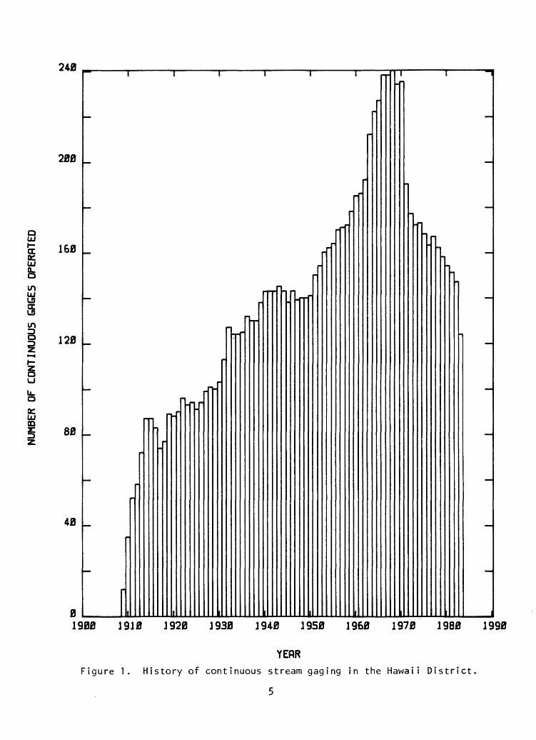
1. History of continuous stream gaging in the Hawaii District 5
2. Mathematical-programing form of the optimization ofthe routing of hydrographers -------------------------- 29
3. Tabular form of the optimization of the routing ofhydrographers - --------------------------------- _____ 30
4. Typical uncertainty function for instantaneous discharge 50
5. Temporal average standard error per stream gage for theState of Hawaii --------------------------------- ____ 55
6. Temporal average standard error per stream gage for theOther Pacific Areas 56
Plate
1. Location of stream gages in the State of Hawaii - In pocket
2. Location of stream gages in the Other Pacific Areas -- In pocket
TABLES
Table
1. Selected hydrologic data for stations
9
10
Hawaii District surface-water program Data-use table ---------------------
Summary of calibration for regression
daily streamflow at selected gage sHawaii District ---- ------- -
Statistics of record reconstruction Residual data for Kawaikoi ---------
Summary of the autocovariance analysis
Summary of the routes that may be used to visit stationsin the State of Hawaii ---------
Summary of the routes that may be used to visit stations
in the Other Pacific Areas -----
Selected results of K-CERA analysis for the State of Hawaii
Selected results of K-CERA analysis for theOther Pacific Areas ------------
in the
modeli ng of mean
ites in the
Page
6
2k
39
51
5358
68
VI
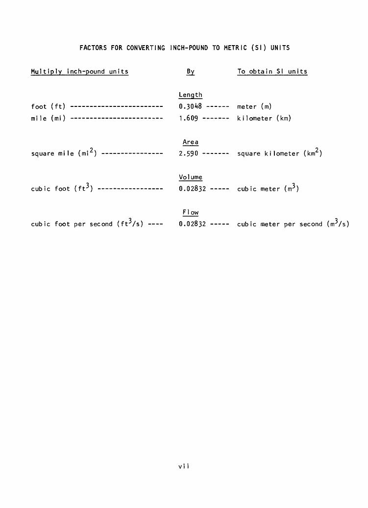
FACTORS FOR CONVERTING INCH-POUND TO METRIC (SI) UNITS
Multiply inch-pound units To obtain SI units
foot (ft)
mi le (mi)
Length
0.3048 meter (m)
1.609 kilometer (km)
2 square mi1e (mi )
Areao
2.590 ---- square kilometer (km )
Volume
cubic foot (ft 3 ) 0.02832 cubic meter (m3 )
Flow3 3
cubic foot per second (ft-Ys) 0.02832 - cubic meter per second (nr/s)
VI I
COST-EFFECTIVENESS OF THE STREAM-GAGING PROGRAM IN THE HAWAII DISTRICT
By I. Matsuoka, R. Lee, and W. 0. Thomas, Jr.
ABSTRACT
This report documents the results of a study of the cost-effectiveness of
the stream-gaging program in the Hawaii District. The stream gages in the
District were divided into two groups, the State of Hawaii and the Other Pacific
Areas. Data uses and funding sources were identified for the 124 continuous
stream gages currently being operated in the Hawaii District with a budget of
$570,620. All the stream gages were identified as having sufficient reason to
continue their operation and they should be maintained in the program for the
foreseeable future.
The current policy for operation of the 92-station program for the State of
Hawaii part of the District program requires a budget of $413,370 per year. The
average standard error of estimate of streamflow records is 21.0 percent. It was
shown that this overall level of accuracy could be improved to 17-7 percent with
the same budget if the gaging resources were redistributed among the gages. A
minimum budget of $370,000 is required to operate the 92-gage program; a budget
less than this does not permit proper service and maintenance of the gages and
recorders. At the minimum budget, the average standard error is 23.7 percent.
The maximum budget analyzed was $550,000, which resulted in an average standard
error of 12.9 percent. Some parts of Hawaii were identified as having very few
or no current streamflow stations. This is a reflection of discontinuing gaging
stations in the past. There are no immediate suggestions for discontinuing or
establishing gages on the basis of this study.
The current policy for operation of the 32-station program for the Other
Pacific Areas part of the District program requires a budget of $157,250 per
year. The average standard error of estimation of streamflow records is 25.9
percent. It was shown that this overall level of accuracy could be improved to
23.2 percent with the same budget if the gac
among the gages. A minimum budget of $1^5,000
ing resources were redistributed
is required to operate the 32-gage
program; a budget less than this does not permit proper service and maintenance
of the gages and recorders. At the minimum budget, the average standard error is
32.0 percent. The maximum budget analyzed was $250,000, which resulted in an
average standard error of 12.2 percent. There
discontinuing or establishing new gaging stati
this time.
NTRODUCTION
The U.S. Geological Survey (USGS) is the
are no immediate suggestions for
ons in the Other Pacific Areas at
principal Federal agency collect
ing surface-water data in the Nation. The collection of these data is a major
activity of the Water Resources Division of the USGS. The data are collected in
cooperation with State and local governments and other Federal agencies. The USGS
is presently (1983) operating approximately
stations throughout the Nation. Some of these
8,000 continuous-record gaging
records extend back to the turn of
the century. Any activity of long standing, such as the collection of surface-
water data, should be reexamined at intervals* if not continuously, because of
changes in objectives, technology, or external constraints. The last systematic
nationwide evaluation of the streamflow information program was completed in
1970 and is documented by Benson and Carter (1973). The USGS is presently (1983)
undertaking another nationwide analysis of the: stream-gaging program that will
be completed over a 5-year period with 20 perc
each year. The objective of this analysis is
cost-effective means of furnishing streamflow
For every continuous-record gaging station, the analysis identifies the
principal uses of the data and relates these
snt of the program being analyzed
to define and document the most
informat ion.
uses to funding sources. Gaged
sites for which data are no longer needed are identified, as are deficient or
unmet data demands. In addition, gaging stations are categorized as to whether
the data are available to users in a real-time sense, on a provisional basis, or
at the end of the water year.
The second aspect of the analysis is t<J> identify less costly alternate
methods of furnishing the needed information; among these are flow-routing
models and statistical methods. The stream-gaging activity no longer is
considered a network of observation points, but rather an integrated information
system in which data are provided both by observation and synthesis.
The final part of the analysis involves the use of Kalman-f i 1 ter ing and
mathematical-programming techniques to define strategies for operation of the
necessary stations that minimize the uncertainty in the streamflow records for
given operating budgets. Kalman-fi1tering techniques are used to compute uncer
tainty functions (relating the standard errors of computation or estimation of
streamflow records to the frequencies of visits to the stream gages) for all
stations in the analysis. A steepest descent optimization program uses these
uncertainty functions, information on practical stream-gaging routes, the
various costs associated with stream gaging, and the total operating budget to
identify the visit frequency for each station that minimizes the overall uncer
tainty in the streamflow. The standard errors of estimate given in the report
are those that would occur if daily discharges were computed through the use of
methods described in this study. No attempt has been made to estimate standard
errors for discharges that are computed by other means. Such errors could differ
from the errors computed in the report. The magnitude and direction of the
differences would be a function of methods used to account for shifting controls
and for estimating discharges during periods of missing record. The stream-
gaging program that results from this analysis will meet the expressed water-data
needs in the most cost-effective manner.
This report is organized into five sections; the first being an introduction
to the stream-gaging activities in the Hawaii District and to the study itself.
The middle three sections each contain discussions of an individual step of the
analysis. Because of the sequential nature of the steps and the dependence of
subsequent steps on the previous results, conclusions are made at the end of each
of the middle three sections. The study, including all conclusions, is summarized
in the final section.
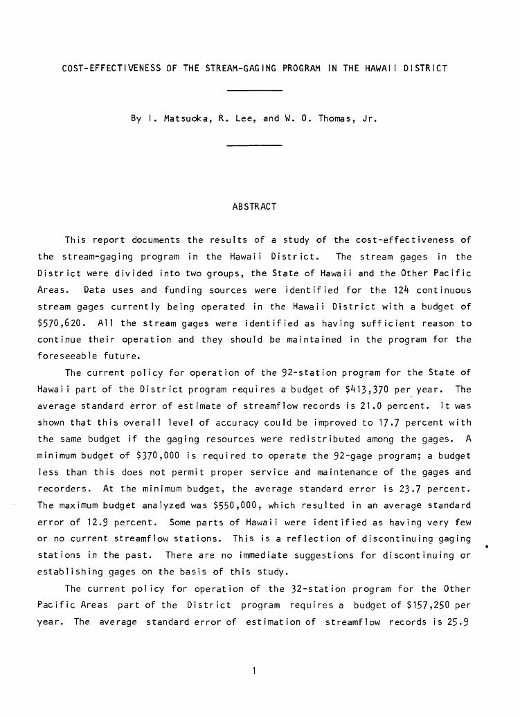
History of the Stream-Gaging Program in the Hawaii District
The program of surface-water investigations by the USGS in the Hawaii Dis
trict has grown rather steadily through the years as Federal and State interests
in water resources increased. The Hawaii office of the USGS began collecting
surface-water data in what is now the State of Hawaii with the establishment of
12 gaging stations in 1909. These first stations were operated primarily to
evaluate the potential of the streams for supply
sugar industry. From this modest beginning, the program rapidly expanded to the
point where, in 1914, the USGS operated 87 gaging stations in the State. During
the next 25 years, the program operated by
increased to 143 gaging stations. Although & small decrease of the program
occurred during the period 1941 to 1950, by 196£l the USGS was operating 240 daily
flow surface-water gaging stations within the Hawaii District. This was the
highest number of stations ever operated by tie Hawaii District. During this
period new programs outside of the State were s
were started in 1952, American Samoa in 1958, snd Okinawa in 1963.
Between 1968 and 1983, there was a net reduction of 116 continuous stream
gages from the Hawaii District gaging program
ing the irrigational needs of the
the Hawaii District gradually
tarted. Gaging stations on Guam
although a new program in the
Trust Territory of the Pacific Islands was started in 1968. Decisions to drop
the gages were based on various economic, technical and political reasons. These
reductions leave the Hawaii District program wi
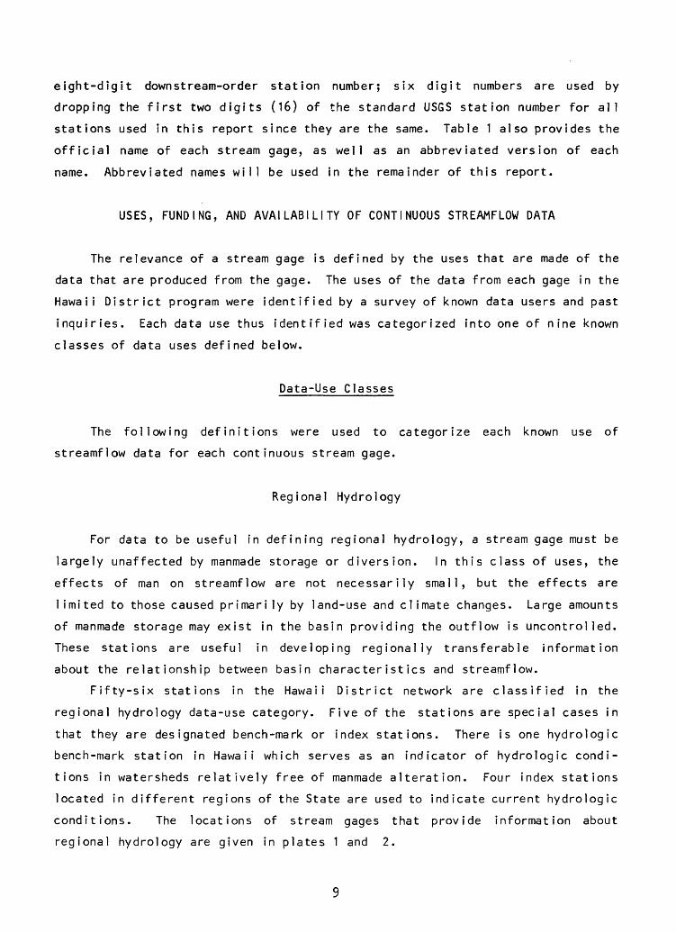
The historical number of continuous stream
District is given in figure 1.
th 124 stations in 1983.
gages operated within the Hawaii
Current Hawaii District Streak-Gaging Program
The stream-gaging network in the Hawaii Dis trict is spread across vast areas
in the Pacific Ocean. The locations of these areas and their political entities
are shown in plates 1 and 2. Ninety-two gages are located in the State of Hawaii,
2 are located in the Commonwealth of the Marianas Island, 7 are in Guam, 4 are in
Palau, 12 are in the Federated States of Micronesia, and 7 are located in
American Samoa. Thirty-two gages located in areas other than the State of Hawaii
will be grouped as stations in the 'Other Pacific Areas'. There are parts of
some islands in which streamflow data sites seem too sparse to provide valid
estimates of streamflow characteristics. This
tinuance of gages in the past for economic, technical and political reasons. The
cost of operating the 124 stream gages in fisca
paucity was caused by discon-
1 year 1983 is $570,620.
Selected hydrologic data, including drainage area, period of record, and
mean annual flow, for the 124 stations are given in table 1. Station identifi
cation numbers used throughout this report are abbreviated from thellSGS's
NUMB
ER OF CONTINUOUS GRGES
OPERRT
ED
-n in c
-t
n> :r
v> rt
O
n
-< O -h O
O u rt U
C
O
c
tn in n
-<
2 3
3
30
tQ
0) to u ID u rt D"
(D IT
0) OJ
0 (/>
rt 1 0 rt
1
ID i > *
ID »_
t9 »_
ID
IO 19
»_
UD lo 19
»_
UD
*>» a
»
UD Ln t9 »»
UD o» t9 !_
ID >J
t9 t-»
UD
G
O a >-
to ID a
t-t-.ro
,**
CD
10
o>
a
s
a
a
a
a
a
i1
1 1
1 1
1 1
! 1
1 1
1
i
k '
L
"^r^
^^ . _
_ __
i
.
H
' 1
.
=1
.~~
^~~*
^^^^
Tr"
*"^
: '
==
==
==
==
==
==
==
==
==
^.,
, _.
..,..
...
-.. --
- -
i-
^^^1
^^ 1
_ , .
, ._
__,
, , ,
,. ...
.ij
- -
- -
-----
- -
- --
....
----- -
.........."
._ .._..."
4
IMl
|
---.
-. «
----
- --
---
-
- -
-----
- _ ̂
.- -
---.
.. -
- -.
--
--- -
- -
TT
- - -
. -
- -
--
,
....... ,,.j
1 1
1 1
1 1
1 1
1 1
1 J
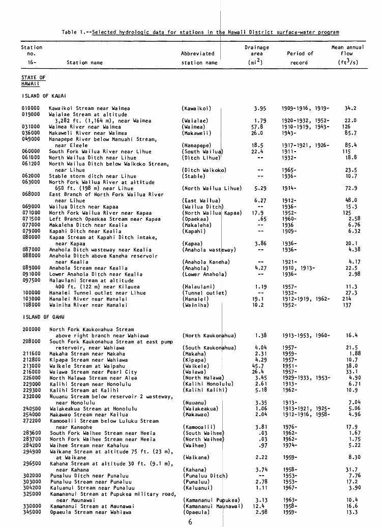
Table 1. Selected hydrologic data for stations in the Hawaii District surface-water program
Station no.16- Station name
Abbreviated
station name
STATE OFHAWAI 1
1 SLAND
010000019000
03100003600001*9000
060000061000061200
062000063000
068000
069000071000071500077000079000080000
087000088000
089000091000097500
100000103000108000
1 SLAND
200000
208000
211600212800213000216000226000229000229300232000
21*0500254000272200
28360028370028420029A900
296500
302000303000301*200325000
3300003A5000
OF KAUAI
Kawaikoi Stream near WaimeaWaialae Stream at altitude
3,282 ft. (1,161* m) f near WaimeaWaimea River near WaimeaMakaweli River near WaimeaHanapepe River below Manuahi Stream,
near EleeleSouth Fork Wailua River near LihueNorth Wailua Ditch near LihueNorth Wailua Ditch below Waikoko Stream,
near LihueStable storm ditch near LihueNorth Fork Wailua River at altitude
650 ft. (198 m) near LihueEast Branch of North Fork Wailua River
near LihueWailua Ditch near KapaaNorth Fork Wailua River near KapaaLeft Branch Opaekaa Stream near KapaaMakaleha Ditch near KealiaKapahi Ditch near KealiaKapaa Stream at Kapahi Ditch intake,
near KapaaAnahola Ditch wasteway near KealiaAnahola Ditch above Kaneha reservoir
near KealiaAnahola Stream near KealiaLower Anahola Ditch near KealiaHalaulani Stream at altitude
1*00 ft. (122 m) near KilaueaHanalei Tunnel outlet near LihueHanalei River near HanaleiWainiha River near Hanalei
OF OAHU
North Fork Kaukonahua Streamabove right branch near Wahiawa
South Fork Kaukonahua Stream at east pumpreservoir, near Wahiawa
Makaha Stream near MakahaKipapa Stream near WahiawaWaikele Stream at WaipahuWaiawa Stream near Pearl CityNorth Halawa Stream near AieaKalihi Stream near HonoluluKalihi Stream at KalihiNuuanu Stream below reservoir 2 wasteway,
near HonoluluWaiakeakua Stream at HonoluluMakawao Stream near KailuaKamooalii Stream below Luluku Stream
near KaneoheSouth Fork Waihee Stream near HeeiaNorth Fork Waihee Stream near HeeiaWaihee Stream near KahaluuWaikane Stream at altitude 75 ft. (23 m) ,
at Wa ikaneKahana Stream at altitude 30 ft. (9.1 m) ,
near KahanaPunaluu Ditch near PunaluuPunaluu Stream near PunaluuKaluanui Stream near PunaluuKamananui Stream at Pupukea military road,
near Maunawa iKamananui Stream at Maunawa iOpaeula Stream near Wahiawa
(Kawa ikoi )
(Waialae)(Waimea)(Makawel i )
(Hanapepe)(South Wailua(Ditch Lihue)
(Ditch Waikok(Stable)
(North Wailua
(East Wailua)(Wailua Ditch(North Wailua(Opaekaa)(Makaleha)(Kapahi)
(Kapaa)(Anahola wast
(Anahola Kane
)
o)
Lihue)
)Kapaa)
eway)
ha)(Anahola)(Lower Anahol
(Halaulani)(Tunnel outle(Hanalei)(Wainiha)
(North Kaukon
(South Kaukon(Makaha)(Kipapa)(Waikele)(Wa iawa)(North Halawa(Kalihi Honol(Kalihi Kalih
(Nuuanu)(Waiakeakua)(Makawao)
( Kamooa 1 i i )(South Waihee(North Waihee(Waihee)
(Waikane)
(Kahana)(Punaluu Ditc(Punaluu)(Kaluanui )
(Kamananui Pu(Kamananui Ma
a)
t)
ahua)
ahua)
ijlu)i)
11
i)
Dukea)jnawai )
(Opaeula)
Drainage area
(mi 2 )
3.95
1.7957.826.0
18.522.1*
--
--
5-29
6.27--
17.9.65 --
3.86
i*.27--
1.19--
19.110.2
1.38
l*.0l*2.311*.29
1*5.726.1*3-*52.615.18
3-351.062.Q1*
3.81.03.03.97
2.22
3.71*--
2.781.11
3.1312.1*2.98
Period of
record
1909-1916, 1919-
1920-1932, 1952-1910-1919, 19*3-19*3-
1917-1921, 1926-1911-1932-
1965-1936-
191*-
1912-1936-1952-1960-1936190S-
1936-1936-
1921-1910, 1913-1936-
1957-1932-1912-1919, 1962-1952-
1913-1953, 1960-
1957-1959-1957-1951-1957-1929-1933, 1953-1913-1962-
1913-1913-1921, 1925-1912-1916, 1958-
1976-1962-1962-197*-
1959-
1958-1953-1953-1967-
1963-1958-1959-
Mean annual flow
(ft3 /s)
3*. 2
22.012685.7
85.*11518.8
23.510.7
72.9
1*8.015.3
1252.586.766.32
20.1i».38
*.1722.52.98
11.327.3
214137
16.*
21.51.88
10.738.033.1*.906.7110.9
7.0*5.06*.96
17.91.671.755.22
8.30
31.77.7617.23.90
10.*16.613.3
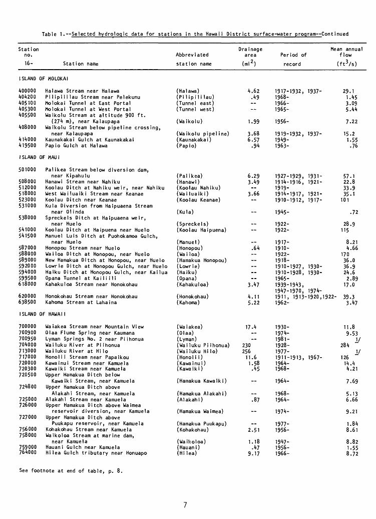
Table 1. Selected hydroloqic data for stations in the Hawaii District surface-water program Continued
Station no.
16- Station name
1 SLAND
400000404200405100405300405500
408000
414000419500
1 SLAND
501000
508000512000518000523000531000
538000
541000541500
587000588000589000592000594000599500618000
620000638500
1 SLAND
700000700900700950704000713000717000720000720300720500
724800
725000726000
727000
756000758000
759000764000
OF MOLOKAI
Halawa Stream near HalawaPilipililau Stream near PelekunuMolokai Tunnel at East PortalMolokai Tunnel at West PortalUaikolu Stream at altitude 900 ft.
(274 m) , near KalaupapaUaikolu Stream below pipeline crossing,
near KalaupapaKaunakakai Gulch at KaunakakaiPapio Gulch at Halawa
OF MAUI
Palikea Stream below diversion dam,near Kipahulu
Hanawi Stream near NahikuKoolau Ditch at Nahiku weir, near NahikuWest Uailuaiki Stream near KeanaeKoolau Ditch near KeanaeKula Diversion from Haipuaena Stream
near 01 i ndaSpreckels Ditch at Haipuaena weir,
near HueloKoolau Ditch at Haipuena near HueloManuel Luis Ditch at Puohokamoa Gulch,
near HueloHonopou Stream near HueloUailoa Ditch at Honopou, near HueloNew Hamakua Ditch at Honopou, near HueloLowrie Ditch at Honopou Gulch, near HueloHaiku Ditch at Honopou Gulch, near KailuaOpana Tunnel at Ka i 1 i i 1 iKahakuloa Stream near Honokohau
Honokohau Stream near HonokohauKahoma Stream at Lahaina
OF HAUAI 1
Uaiakea Stream near Mountain ViewOlaa Flume Spring near KaumanaLyman Springs No. 2 near PiihonuaUailuku River at PiihonuaUailuku River at Hi loHonolii Stream near PapaikouKawainui Stream near KamuelaKawaiki Stream near KamuelaUpper Hamakua Ditch below
Kawaiki Stream, near KamuelaUpper Hamakua Ditch above
Alakahi Stream, near KamuelaAlakahi Stream near KamuelaUpper Hamakua Ditch above Uaimea
reservoir diversion, near KamuelaUpper Hamakua Ditch above
Puukapu reservoir, near KamuelaKohakohau Stream near KamuelaUaikoloa Stream at marine dam,
near KamuelaHauani Gulch near KamuelaHi lea Gulch tributary near Honuapo
Abbreviated
station name
(Halawa)(Pi 1 ipi 1 i lau)(Tunnel east)(Tunnel west)
(Uaikolu)
(Uaikolu pipeline)(Kaunakakai)(Papio)
(Palikea)(Hanawi)(Koolau Nahiku)(Uailuaiki)(Koolau Keanae)
(Kula)
(Spreckels)(Koolau Haipuena)
(Manuel)(Honopou)(Uailoa)(Hamakua Honopou)(Lowr ie)(Haiku)(Opana)(Kahakuloa)
(Honokohau)(Kahoma)
(Wa iakea)(Olaa)(Lyman)(Wa i luku Pi ihonua)(Uailuku Hilo)(Honol i i )( Kawa i nu i )(Kawa iki )
(Hamakua Kawaiki)
(Hamakua Alakahi)(Alakahi)
(Hamakua Uaimea)
(Hamakua Puukapu)(Kohakohau)
(Uaikoloa)(Hauani)(Hi lea)
Dra inage area
(mi 2 )
4.62.49 --
1.99
3.686.57.94
6.293.49
3.66
.64
3.47
4.115.22
17.4~
23025611.61.58.45
.87
2.51
1.18.47
9.17
Mean annual Period of flow
record (ft 3 /s)
1917-1932,1968-1966-1965-
1956-
1919-1932,1949-1963-
1927-1929,1914-1916,1919-1914-1917,1910-1912,
1945-
1922-1922-
1917-1910-1922-1918-1910-1927,1910-1928,1965-1939-1943,1947-1970,
1937-
1937-
1931-1921-
1921-1917-
1930-1930-
1974-1911, 1913-1920,1922-1962-
1930-1974-1981-1928-1977-1911-1913,1964-1968-
1964-
1968-1964-
1974-
1977-1956-
1947-1956-1966-
1967-
29.11.453.095.44
7.22
15.21.55.76
57.122.833.935.1
101
.72
28.9115
8.214.66
17036.036.924.62.8917.0
39.33.47
11.89.53
I/284
I/126 ~14.44.21
7.69
5.136.66
9.21
1.848.61
8.821.558.72
See footnote at end of table, p. 8.
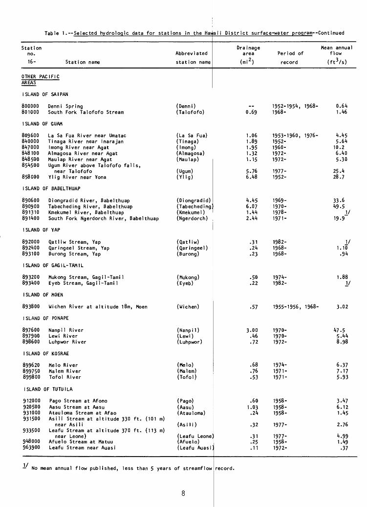
Table 1. Selected hydroloqic data for stations in the HaviaIi District surface-water program--Continued
Station no.
16- Station name
OTHER PACIFICAREAS
ISLAND OF SAIPAN
800000 Denni Spring801000 South Fork Talofofo Stream
ISLAND OF GUAM
809600 La Sa Fua River near Umatac840000 Tinaga River near Inarajan847000 Imong River near Agat848100 Almagosa River near Agat848500 Maulap River near Agat854500 Ugum River above Talofofo falls,
near Talofofo858000 Ylig River near Yona
ISLAND OF BABELTHUAP
890600 Diongradid River, Babelthuap 890900 Tabecheding River, Babelthuap 891310 Kmekumel River, Babelthuap891400 South Fork Ngerdorch River, Babelthuap
ISLAND OF YAP
892000 Qatliw Stream, Yap892400 Qaringeel Stream, Yap893100 Burong Stream, Yap
ISLAND OF GAG 1 L- TAMIL
893200 Mukong Stream, Gag il -Tamil893400 Eyeb Stream, Gag il -Tamil
ISLAND OF MOEN
893800 Wichen River at altitude l8m, Moen
ISLAND OF PONAPE
897600 Nanpil River897900 Lew! River898600 Luhpwor River
ISLAND OF KOSRAE
899620 Melo River899750 Malem River899800 Tofol River
ISLAND OF TUTU 1 LA
912000 Pago Stream at Afono920500 Aasu Stream at Aasu931000 Atauloma Stream at Afao931500 Asili Stream at altitude 330 ft. (101 m)
near Asi 1 i933500 Leafu Stream at altitude 370 ft. (113 m)
near Leone)948000 Afuelo Stream at Matuu963900 Leafu Stream near Auasi
Abbreviated
station name
(Denni)(Talofofo)
(La Sa Fua)(Tinaga)( Imong)(Almagosa)(Maulap)
(Ugum)(Ylig)
(Diongradid) (Tabechedingl (Kmekumel )(Ngerdorch)
(Qatliw)(Qaringeel)(Burong)
(Mukong)(Eyeb)
(Wichen)
(Nanpil)(Lew!)(Luhpwor)
(Melo)(Malem)(Tofol)
(Pago)(Aasu)(Atauloma)
(Asili)
(Leafu Leone(Afuelo)(Leafu Auasi
Dra inage area
(mi 2 )
_.0.69
1.061.891.951.321.15
5.766.48
4.45 6.07 1.442.44
.31
.24
.23
.50
.22
.57
3.00.46.72
.68
.76
.53
.601.03.24
.32
.31
.25
.11
Period of
record
1952-1954, 1968-1968-
1953-1960, 1976-1952-1960-1972-1972-
1977-1952-
1969- 1970- 1978-1971-
1982-1968-1968-
1974-1982-
1955-1956, 1968-
1970-1970-1972-
1974-1971-1971-
1958-1958-1958-
1977-
1977-1958-1972-
Mean annual flow
(ft 3 /s)
0.641.46
4.455.6410.26.405-30
25.428.7
33.6 49.5
1/19-9
1/1.10.94
1.88V
3.02
47.55.448.98
6.377.175-93
3.476.121.45
2.76
4.991.49.37
No mean annual flow published, less than 5 years of streamflow record.
eight-digit downstream-order station number; six digit numbers are used by
dropping the first two digits (16) of the standard USGS station number for all
stations used in this report since they are the same. Table 1 also provides the
official name of each stream gage, as well as an abbreviated version of each
name. Abbreviated names will be used in the remainder of this report.
USES, FUNDING, AND AVAILABILITY OF CONTINUOUS STREAMFLOW DATA
The relevance of a stream gage is defined by the uses that are made of the
data that are produced from the gage. The uses of the data from each gage in the
Hawaii District program were identified by a survey of known data users and past
inquiries. Each data use thus identified was categorized into one of nine known
classes of data uses defined below.
Data-Use Classes
The following definitions were used to categorize each known use of
streamflow data for each continuous stream gage.
Regional Hydrology
For data to be useful in defining regional hydrology, a stream gage must be
largely unaffected by manmade storage or diversion. In this class of uses, the
effects of man on streamflow are not necessarily small, but the effects are
limited to those caused primarily by land-use and climate changes. Large amounts
of manmade storage may exist in the basin providing the outflow is uncontrolled.
These stations are useful in developing regionally transferable information
about the relationship between basin characteristics and streamflow.
Fifty-six stations in the Hawaii District network are classified in the
regional hydrology data-use category. Five of the stations are special cases in
that they are designated bench-mark or index stations. There is one hydrologic
bench-mark station in Hawaii which serves as an indicator of hydrologic condi
tions in watersheds relatively free of manmade alteration. Four index stations
located in different regions of the State are used to indicate current hydrologic
conditions. The locations of stream gages that provide information about
regional hydrology are given in plates 1 and 2.
Hydrologic Systems
thatStations that can be used for accounting,
logic conditions and the sources, sinks, and fl
systems including regulated systems, are des
stations. They include diversions and return flows
for defining the interaction of water systems.
The bench-mark and index stations are a
systems category because they are accounting
tions of the hydrologic systems that they gage.
There are sixty-five stations in the Hawaii
operated to evaluate hydrologic systems.
is, to define current hydro-
jxes of water through hydrologic
ignated as hydrologic systems
and stations that are useful
for
Legal Obligation
the verification or enforcement
The legal obligation category
required to operate to satisfy a
Some stations provide records of flows for
of existing treaties, compacts, and decrees,
contains only those stations that the USGS is
legal responsibility.
There are no stations in the Hawaii District program that exist to fulfill a
legal responsibility of the USGS.
Planning and Design
Gaging stations in this category of data u
design of a specific project (for example, a d
system, water-supply diversion, hydropower plant
or group of structures. The planning and desi
stations that were instituted for such purposes
valid.
Currently, one station in the Hawaii District program is being operated for
planning and design purposes.
so included in the hydrologic
current and long-term condi-
District program that are being
cim
se are used for the planning and
, levee, floodwall, navigation
, or waste-treatment facility)
gn category is limited to those
and where this purpose is still
10
Project Operation
Gaging stations in this category are used, on an ongoing basis, to assist
water managers in making operational decisions such as reservoir releases,
hydropower operations, or diversions. The project operation use generally
implies that the data are routinely available to the operators on a rapid-
reporting basis. For projects on large streams, data may only be needed every
few days.
There are no stations in the Hawaii District program that are used in this
manner.
Hydrologic Forecasts
Gaging stations in this category are regularly used to provide information
for hydrologic forecasting. These might be flood forecasts for a specific river
reach, or periodic (daily, weekly, monthly, or seasonal) flow-volume forecasts
for a specific site or region. The hydrologic forecast use generally implies
that the data are routinely available to the forecasters on a rapid-reporting
basis. On large streams, data may only be needed every few days.
There are no stations in the Hawaii District program that are in the hydro-
logic forecast category.
Water-Quality Monitoring
Gaging stations where regular water-quality or sediment-transport monitor
ing is being conducted and where the availability of streamflow data contributes
to the utility or is essential to the interpretation of the water-quality or
sediment data are designated as water-quality-monitoring sites.
One such station in the program is a designated bench-mark station and six
are National Stream Quality Accounting Network (NASQAN) stations. Water-quality
samples from bench-mark stations are used to indicate water-quality charac
teristics of streams that have been and probably will continue to be relatively
free of manmade influence. NASQAN stations are part of a country-wide network
designed to assess water-quality trends of significant streams.
11
Research
Gaging stations in this category are operated for a particular research or
water-investigations study. Typically, these are only operated for a few years
There are no stations in the Hawaii District program used in the support of
research activities.
Other
In addition to the eight data-use classes described above, data in this
category are used to provide information on floods by furnishing flood hydro-
graphs peak stages and discharges to the cooperator. There are five such
stations in the Hawaii District program.
Fund ing
The three sources of funding for the strearrfl
1. Federal program. Funds that have been
2. Other Federal Agency (OFA) program. Funds
the USGS by OFA's.
3. Co-op program. Funds that come jointly
funding and from any non-Federal cooperating ag
may be in the form of direct services or cash.
In all three categories, the identified
the collection of streamflow data; sources of
particularly collection of water-quality sample
the site may not necessarily be the same as thos
Currently, 13 entities are contributing
stream-gaging program.
rom USGS cooperative-designated
sncy. Cooperating agency funds
sources
ow-data program are:
directly allocated to the USGS.
that have been transferred to
of funding pertain only to
funding for other activities,
, that might be carried out at
e identified herein.
funds to the Hawaii District
12
Frequency of Data Availability
Frequency of data availability refers to the times at which the streamflow
data may be furnished to the users. In this category, three distinct possibili
ties exist. Data can be furnished by direct-access telemetry equipment for
immediate use, by periodic release of provisional data, or in publication format
through the annual data report published by the USGS for Hawaii and Other Pacific
Areas (U.S. Geological Survey, 1981). In the current Hawaii District program,
data for all 124 stations are made available through the annual report and is
designated A in table 2.
Data-Use Presentation
Data-use and ancillary information are presented for each continuous gaging
station in table 2, which is replete with footnotes to expand the information
conveyed. The entry of an asterisk in the table indicates that no footnote is
requi red.
Conclusions Pertaining to Data Uses
A review of the data-use and funding information presented in table 2
supports the continuation of all the existing stations. Therefore, all the 124
gaging stations will be considered in the next step of this analysis.
13
->J
ON
U1
4^
\uO
N
> »
c: z
s -
o co
r-
>
O
-J
O
rt
- O
CO
CO
ZJ
-1
£
Q)
ZJ
<
O
fl>
rt
CQ
>
rt C
Q
-«
fD
I 0
Z
O
0>
rt
O
-1
rt
0>
O
fl>
-«
(/>
-.-.
ZJ
-h
-j
O
rt 3
O
CL
3
U)
Q)
CQ
3
JC
rt
_.
Q)
_.
O
O
C
-I
£
3
-h O
-h
t/>
-i
Q>
CL
n
n>
n>ID
.
-h
(Q
X
ZJ
Q)
(Q
O
rt
CQ
O
Q)
ZJ
CL
O
U3
(D
U
n>
Q
. n
-1
0)
C
(Q
U)
rt
u>
cu
n>
tn
rt
Q
) rt O ZJ
jr-
_*_
»_
»
CD
C
D
0 0
0
U>
\J3
OO
\jO
C
D "
^J »
CD
C
D O
V/l
C
D
CD
O
O
C
D O
C
D
CD
C
D
CD
C
D
*
*
4^
-C
-
<J1
->J
s>
ro r
o ro
> >
> >
>
CD
C
D
CD
C
D
CD
O
O O
O
OO
O
O--
J
U>
C
XJ-
^J
CD
VJD
C
D
CD
O
C
D
CD
C
D
CD
O
C
D
CD
C
D
CD
C
D
CD
C
D
*
4=-
*
«
-C-
ro s
> s>
ro
ro
> >
> >
>
CD
C
D
CD
C
D
CD
->
J "^
J -^
J O
N
ON
-«
J
_»
_» U
>
OO
C
D V
/l
CD
C
D
CD
C
D
CD
C
D
CD
C
D
CD
C
D
CD
C
D
CD
»
'
-C-
4=
-~
4^
vn - j
N> r
o ro
ro
> >
> >
>
CD
C
D
CD
C
D
CD
O
"^ O
^ O
"^ O
"^ O
"^\uO
ro » »
CDC
D
CD
C
O
CD
C
D
CD
O
C
D
CD
C
D
CD
C
D
CD
C
D
CD
>}
4>
\uO
\u
O
>}-
CO
C
O
CO
C
O
CO
> >
>
>
>
CD
C
D
CD
C
D
CD
JC
C
O
4>
\uO
\u
O » »
J>
I
U>
O
N -»
VJ
D 0
SI
>
O
CD
C
D
CD
C
D
3>
|
CD
C
D
CD
C
D O
|T)
CD
C
D
CD
O
O
O ~n
>}
X-
>f.
}}.
;}-
4>
ON #
>}
ro r
o ro
> >
> >
>
CO rt
D
Q)
O
rt O ZJ
Reg
ion
al
Hyd
rolo
gy
Hyd
rolo
gic
Sys
tem
s
Leg
al
Ob
lig
ati
on
s
Pla
nn
ing
an
d D
esig
n
Pro
ject
Op
era
tio
n
Hyd
rolo
gic
F
ore
casts
Wate
r-Q
uality
M
on
ito
rin
g
Res
earc
h
Oth
er
Fed
eral
P
rog
ram
OF
A
Pro
gra
m
Co
-Op
P
rog
ram
o
>
i
> c: CO m ~n c:
z.
o z.
0
Fre
qu
ency
of
D
ata
Av
ail
ab
ilit
y
-\ Q)
CT n>
ro i i CJ
Q)
rt
Q) I C
U) n> rt
Q) n>
o <
/> c
z
n
>
>rt
Q_
(/)
(/)
i*"
>QJ
n> o z
D D
oQ
. rt
-i
O1
T3
rt
O rt
01
QJO
"I
rt
C
QJ
O
D
3
-h
Ort
01
D^<
~o
m
o
3O
-i
IQ
-h
rt .
rt
IQ
O
QJ-1
rt
O o^ c
c i DO
O
QJ -1
0.
O -h QJ
rt
fl> to C -o -o
O
O
Q.
Q.
QJ
rt
QJ
rt
OQJ
D
rt
tQ(D
I rt
O
(t> h
-I
3
o:
QJ
_.
Q)
DL n
> X
01 rt
QJ
rt
VjO
V
jO
VjO
VjO
-C
- Vu
O N
J O
V
/l O
U1 -t
- O
O
O
N
>
O O
O
O
O
O
O
O
5!-
S{-
>!
5!-
NJ
N
J V
O U
>
> >
>
>
VjO
V
jO
NJ
N
J
N>
O
O
V
O
VO
C
O
VjJ
N
J
ON
-fc
- -f
e-
Ci
O U
l V
O
INJ
O 0
O
O
O
O
O
O
O
0
«
5!-
X- -f
*
VD
V
D
NJ
N
J V
D
> >
>
>
>
NJ
N
J
N>
N
J
NJ
O
O
OO
->J
U
1 -f
VjO
V
jO
N>
-fc
~ O
-
J
ON
NJ
O
U1
O
O
O
O
O
O
O
O
O
O
«
>!-
JS-
>!
OO
>J
VD
V
D
NJ
VT>
> >
> >
>
NJ
N
J
Ni
NJ
N
>
VjO
N
>
Ni
NJ
»
N>
VD
VD
O
N O
N
O V
jO O
O
O
O
O
O
0
O
O
O
O
O
O
>!
si-
>!
ON
U1 *
->J
VD
N
J
NJ
N
J
> >
>
>
>
NJ
N
J
N>
N
>
N>
»
* *
C3
C3
VjO
N
J »
OO
O
0
OO
CT»
0
0
O
O
O
O
O
O
O
O
C
b O
*
5!-
* *
ON *
NJ
N
>
N>
N
3
> >
>
>
>
</>
rt
rj
ojO
rt
O rj
Re
gio
na
l H
yd
rolo
gy
Hy
dro
log
ic
Sys
tem
s
Le
ga
l O
blig
ati
on
s
Pla
nn
ing
an
d
De
sig
n
Pro
jec
t O
pe
rati
on
Hy
dro
log
ic
Fo
recasts
Wa
ter-
Qu
ali
ty
Mo
nit
ori
ng
Re
se
arc
h
Oth
er
Fed
era
l P
rog
ram
OF
A
Pro
gra
m
Co
-Op
Pro
gra
m
o > > c: </>
m TI
c:
z 0 z.
CD
Fre
qu
en
cy
o
f D
ata
A
vailab
ilit
y
QJ
CT n> NJ I I o QJ
rt
QJ I C
O1 n> QJ
cr n> i i o
O c
fl>
O.
»
O ^
J
ON
U1
-tr
N) »
-
o c:
z 2
c
/> i
-t
O
J>
O
-»
rt
O
-»S
!c/>
C/)
a-»Q
JD
fl>
<
O rt
(O
C
O
-»
J>
rt
to
CD
i
rt
O
~i
rt
O
H>
_.
_.
-i
w
_.
_.
-h
-j
O
"I
TJ
rt
D
O
3
3
-i
u>
Q)
to
3
x
rt
Q)
-.
ID
tQ
O O
CS
S
DD
-h
O-h
wQ
JQ
-
O.
rt
3
(T>
(T> m
-h
x
Q.
O
^
O
3
CO
O
u»
3 -
O
rt
(T>
3
Q.
03
U)
Q)
(T>
rt
rt 3
(T)
Q.
Q.
-i
03
O
O
U)
rt
D
CO
*
U)
3n>
o>
U) rt 0 c U)
(D
ON
V^
J C
»
vn C3
C3
Ul
^J >
ON
CT
.U1 U
l U
lro
» v
u VD
vu
o O
OVD
^-
roC
D O
Ul
C3
C3
o o
o o
o
o o
o o
o
*
5t-
-t-
^*
ON «
ro
ro r
o ro
> >
> >
>
ui
un u
i u
i u
iC
O C
O C
O .
£-
.fc-
vu o
o^J
» »
^ O
O
V-T
1 ^
O
O
O
O
O
o o
o o
o
-
_fc-
O »
Jr-
C3
ro r
o ro
ro
ro
> >
> >
>
Ul
VJl
Ul
V/1
Ul
vjo
\jj
ro » »
oo »
vja
oo r
oC
3 C
D O
O
O
o o
o
o o
o
o o
o o
«
»
_» o
o
ro r
o ro
ro
ro
> >
> >
>
U1 U
i Jr-
^-
4^
o o
» » o
oo
_a
vr>
-t-
c»C
3 C
3 U
l O
O
o o
o o
o
o o
o o
o
* *
«
«
Ul
^J
ro r
o ro
ro
> >
> >
>
^r
4r-
4^
^-
^r
o o
o
o
oU
1 U
l U
l 4
> 0
ui
vjo »
ro o
o
o o
o o
o
o o
o o
«
st-
* -
fc- -f
c-
ON
ro r
o ro
ro
ro
> >
> >
>
to rt
3
£U
O
rt o' 3
Reg
ion
al
Hy
dro
log
y
Hyd
rolo
gic
S
yste
ms
Leg
al
Ob
ligat
ion
s
Pla
nn
ing
an
d
Des
ign
Pro
ject
Op
erat
ion
Hyd
rolo
gic
F
ore
cast
s
Wate
r-Q
uality
M
on
ito
rin
g
Res
earc
h
Oth
er
Fed
eral
Pro
gram
OFA
P
rog
ram
Co
-Op
Pro
gram
Fre
qu
ency
o
f D
ata
Availab
ilit
y
o > > c:
to
m TI
c:
z
o z o
1 03 cr n> ro
i o Q)
rt 03 C
U) n> rt 03 cr n> i i o O 3
rt 3
C n> Q.
N)
-fc-
N
) »
IE O
Z
CO |
<
O
>
-I
r+
OQ
_ 3
CO
-1
£U
3
i
(T>
<O
r+
IQ
o </>
^ to
n>
i
r+
Z £
U r+
O
r+
O
<T>IQ
O
(fl
-h 1
r+
O
3o
c cu
-3 :r
Cft
r+
cu .
cr n
> c
S
ufl>
O
(/>
d)
Q-
3 0>
0>O rr QJ
1
7T to
r+
QJ
_. x
*vj -
^J
ON v
n^r V
jO
O O
O
O
0
0
Jf-
*
hO
N)
">
">
^J
-^J
-^J
-^J
-^J
vn v
n N>
N>
N>
OO
QN
-^J
ON
\n
o o
o o
o
o o
o o
o
a o
o o
o
*
jf-
-fc-
-fc
- jf-
NJ
N)
N)
hO
N)
> >
>
>
>
-J -^
J -^
J ->
J -J
N
) N
) N
) N
) »
^r O
O
O
-^J
O
O \
Tt
*u>J
O
O
O
O
O
O
O
O
O
O
O
O <u
O
-fc-
-f
c-
jf-
jf- ^ *u
O 5t-
N)
N)
N)
N)
> >
>
>
>
-J -
^J -
>J
-J -
^J
»
O O
O
O
Vj
O
-Cr O
O
O
O
O
V£>
U3
C
3 C
3 C
3 VJ
1 C
3 C
3 C
3 O
O
O
O -*
* *
N> '
ON Jf-
N)
NJ
N)
N)
> >
>
>
>
CO
r+
3
£U
O
rh O 3
Re
gio
na
l H
ydro
log
y
Hyd
rolo
gic
S
yste
ms
Lega
l O
blig
atio
ns
Pla
nnin
g an
d D
esig
n
Pro
ject
Ope
ratio
n
Hyd
rolo
gic
Fore
cast
s
Wate
r-Q
ualit
y M
on
itorin
g
Re
sea
rch
Oth
er
Fed
eral
P
rogr
am
OFA
P
rogr
am
Co-
Op
Pro
gra
m
0 >
> c:
CO m ~n c:
z 0 z:
o
Fre
quen
cy o
f D
ata
Ava
ilabili
ty
QJ cr o QJ QJ cr n> i i o
o 3 3 c n> Q.
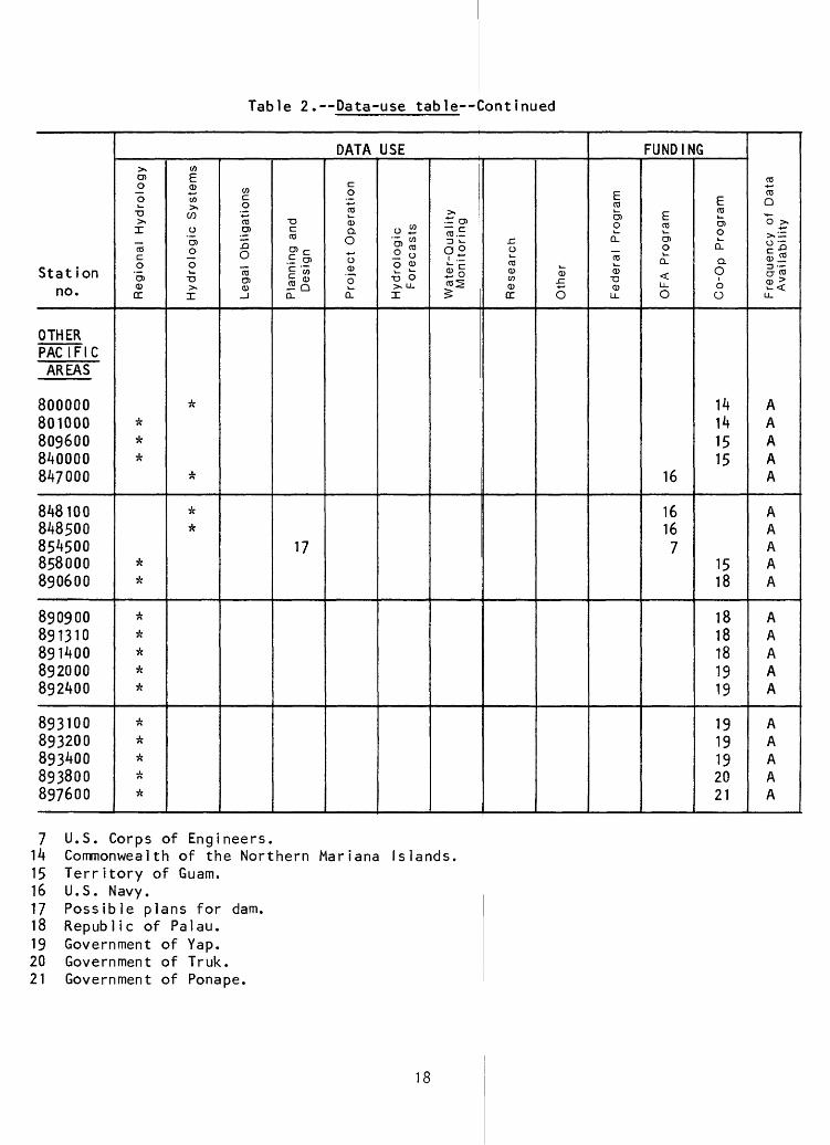
Table 2. Data-use table Continued
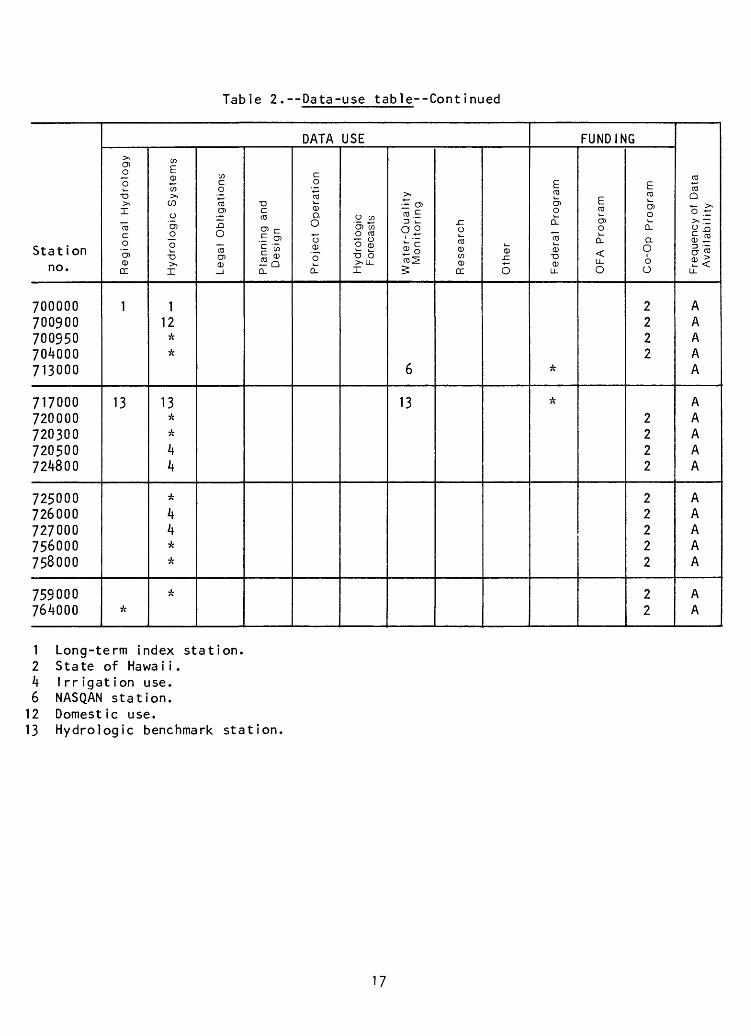
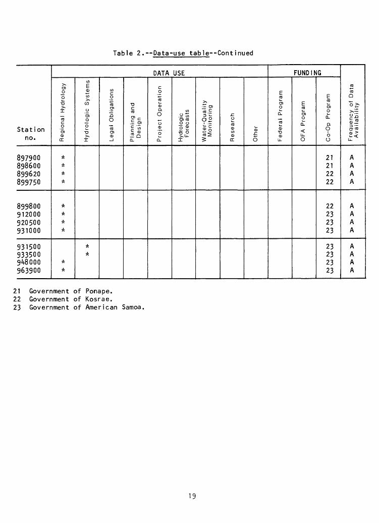
Station no.
OTHERPACIFICAREAS
800000801000809600840000847000
848100848500854500858000890600
890900891310891400892000892400
893100893200893400893800897600
DATA USE..^O)0oU.
T3>\I
Regional
***
**
**JL
*
JL
JL
*
*
JL
*
OTEo>OT
W
0
Hydrologi
*
*
**
c oCDg>
O "coO) 0)
oc
Planning a Design
17
coCD
CDa0
oQ) 0
CL
0 £
Hydrologi Forecas
j>.. O)~ c
Water-Qui Monitor!Research
Q).c6
FUNDING
E roO)o
Federal P
ECD
O) O
CL
U_O
16
16167
ECD
O)O
CL
a O o O
14141515
1518
1818181919
1919192021
CD
CD Q
"o >..t^
Frequencv Availabil
AAAAA
AAAAA
AAAAA
AAAAA
7 U.S. Corps of Engineers.14 Commonwealth of the Northern Mariana15 Territory of Guam.16 U.S. Navy.17 Possible plans for dam.18 Republic of Palau.19 Government of Yap.20 Government of Truk.21 Government of Ponape.
Is lands.
18
G">
CD
CD
O
O
O
333
n>
n>
n>
o
o
o
30
0fl>
(fl -3
O
fl>
fl>Q
)
en OJ
3
O
OJ
U>
U>
VO
VO
O
^ -t
-v>
J V
-o
VjO
O
OV
A) »
u> o
^n
ui
C3
C3
CD
C
D
CD
C
D
CD
C
D
>(
*
*
5(-
N>
|s>
|s>
N>
VA>
VjO
VA>
VA>
> >
>
>
U)
VJ3
U>
C
O
OO
|S
> »
U)
-»
C3
|s>
U)
CD
U1
CD
C
O
CD
C
D
CD
O
O
C
D
CD
C
D
x-
«
>(
a-
N>
|s>
|s>
N>
OO
V
A>
OO
|S
>
> >
>
>
CO
CO
CO
CO
V^
> U
) U
> U
)u>
u>
co*»
g*-
J
ON
CT
»U
)vn
N>
CD o
CD
C
D
CD
C
D
*
>(
>(
>t-
|S>
|S
>
|S>
N
>|s
> N
> -»
> >
> >
to rt-
=}
0)
0
M-
O u
Re
gio
na
l H
ydro
log
y
Hyd
rolo
gic
S
yste
ms
Legal
Oblig
atio
ns
Pla
nn
ing
and
De
sig
n
Pro
ject
Op
era
tio
n
Hyd
rolo
gic
F
ore
cast
s
Wa
ter-
Qu
alit
y
Mo
nito
rin
g
Re
sea
rch
Oth
er
Fe
de
ral
Pro
gra
m
OF
A
Pro
gra
m
Co-O
p
Pro
gra
m
o > > cz
Co
m ~n cz
z.
o z.
o
Fre
quency
of
Da
ta
Availa
bili
ty
0) cr o 0) 0) cr o o 3 =1
C
(D
Q.
ALTERNATIVE METHODS OF DEVELOPING ST
The second step of the analysis of the stream-gaging program is to investi
gate alternative methods of providing daily streamflow information in lieu of
operating continuous-flow gaging stations. The
identify gaging stations where alternative technology, such as flow-routing or
statistical methods, will provide information a^out daily mean streamflow in a
continuous stream gage. Nomore cost-effective manner than operating a
guidelines concerning suitable accuracies exist
therefore, judgment is required in deciding whether the accuracy of the estimated
daily flows is suitable for the intended purpos
will influence whether a site has potential
example, those stations for which flood hydrogra
sense, such as hydrologic forecasts and project ©Deration, are not candidates for
the alternative methods. Likewise, there might lie a legal obligation to operate
an actual gaging station that would preclude uti
primary candidates for alternative methods are stations that are operated
<EAMFLOW INFORMATION
objective of the analysis is to
or particular uses of the data;
The data uses at a station
for alternative methods. For
phs are required in a real-time
izing alternative methods. The
upstream or downstream of other stations on the s
estimated streamflow at these sites may be
ame stream. The accuracy of the
suitable because of the high
redundancy of flow information between sites. Similar watersheds, located in the
same physiographic and climatic area, also may
methods.
All stations in the Hawaii District stream-
as to their potential utilization of alternative
was applied at seven stations. The selection of gaging stations and the applica
tion of the specific method are described in subs
have potential for alternative
gaging program were categorized
methods and one selected method
equent sections of this report.
This section briefly describes the alternative method used in the Hawaii District
analysis and documents why this specific method was chosen.
Because of the short timeframe of this analysis, only two methods were
considered: multiple-regression analysis and f
attributes of a proposed alternative method are (1) the proposed method should be
computer oriented and easy to apply, (2) the proposed method should have an
available interface with the USGS WATSTORE Daily
low-routing model. Desirable
Values File (Hutchinson, 1975),
(3) the proposed method should be technically sound and generally acceptable to
the hydrologic community, and (4) the proposed method should permit easy
20
evaluation of the accuracy of the simulated streamflow records. The desirability
of the first attribute above is rather obvious. Second, the interface with the
WATSTORE Daily Values File is needed to easily calibrate the proposed alternative
method. Third, the alternative method selected for analysis must be technically
sound or it will not be able to provide data of suitable accuracy. Fourth, the
alternative method should provide an estimate of the accuracy of the streamflow
to judge the adequacy of the simulated data.
The time of travel of flow between upstream and downstream gaging stations
in the Hawaii District is measured in hours, often in minutes, rather than days.
This together with the fact that there are few streams with upstream and
downstream gages made the flow-routing model impractical. Therefore, of the two
methods that were considered only the multiple regression analysis was used.
Description of Regression Analysis
Simple- and multiple-regression techniques can be used to estimate daily
flow records. Regression equations can be computed that relate daily flows (or
their logarithms) at a single station to daily flows at a combination of
upstream, downstream, and (or) tributary stations. This statistical method is
not limited, like the flow-routing method, to stations where an upstream station
exists on the same stream. The explanatory variables in the regression analysis
can be stations from different watersheds, or downstream and tributary water
sheds. The regression method has many favorable attributes in that it is easy to
apply, provides indices of accuracy, and is generally accepted as a good tool for
estimation. The theory and assumptions of regression analysis are described in
several textbooks such as those by Draper and Smith (1966) and Kleinbaum and
Kupper (1978). The application of regression analysis to hydrologic problems is
described and illustrated by Riggs (1973) and Thomas and Benson (1970). Only a
brief description of regression analysis is provided in this report.
21
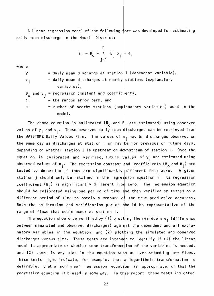
A linear regression model of the following form was developed for estimating
daily mean discharge in the Hawaii District:
Y, = Bo + Z + e.
where
y. = daily mean discharge at station
x. = daily mean discharges at nearby
var iables),
B and B. = regression constant and coeffic
e. = the random error term, and
p = number of nearby stations (exp
model.
The above equation is calibrated (B and B
values of y. and x.. These observed daily mean
the WATSTORE Daily Values File. The values of
the same day as discharges at station i or may
depending on whether station j is upstream or downstream of station i. Once the
equation is calibrated and verified, future v
observed values of x.. The regression constant
tested to determine if they are significantly
station j should only be retained in the regres
coefficient (B.) is significantly different from zero. The regression equation
should be calibrated using one period of time a
different period of time to obtain a measure o
Both the calibration and verification period s
range of flows that could occur at station i.
The equation should be verified by (1) plott
i (dependent variable),
stations (explanatory
ents,
anatory variables) used in the
. are estimated) using observed
ischarges can be retrieved from
. may be discharges observed onJ be for previous or future days,
alues of y. are estimated using
and coefficients (B and B.) are
different from zero. A given
sion equation if its regression
nd then verified or tested on a
: the true predictive accuracy,
hould be representative of the
ing the residuals e. (difference
between simulated and observed discharges) against the dependent and all expla
natory variables in the equation, and (2) plotting the simulated and observed
discharges versus time. These tests are intended to identify if (1) the linear
model is appropriate or whether some transformation of the variables is needed,
and (2) there is any bias in the equation such as overestimating low flows.
These tests might indicate, for example, that a logarithmic transformation is
desirable, that a nonlinear regression equatibn is appropriate, or that the
regression equation is biased in someway. In this report these tests indicated
22
that a linear model with y. and x., in cubic feet per second, was appropriate.
The application of linear-regression techniques to seven watersheds in the
Hawaii District is described in a subsequent section of this report.
It should be noted that the use of a regression relation to synthesize data
at discontinued gaging station entails a reduction in the variance of the stream-
flow record relative to that which would be computed from an actual record of
streamflow at the site. The reduction in variance expressed as a fraction is
approximately equal to one minus the square of the correlation coefficient that
results from the regression analysis.
Categorization of Stream Gages by Their Potential for Alternative Methods
Seven stations were selected for analysis because daily discharges at these
stations were highly correlated with those for some other stations. These seven
stations are Makaweli (036000), North Wailua Kapaa (071000), Hanawi (508000),
Koolau Keanae (523000), Wailuku Piihonua (704000), Kawainui (720000), and
Kawaiki (720300). It should be noted that a high degree of correlation between
stations does not necessarily mean that a high percentage of simulated daily
flows will be within a small percentage, such as 10 percent, of the observed
flows. Regression methods were applied to all seven sites.
Regression Analysis Results
Linear regression techniques were applied to the seven selected sites. The
streamflow record for each station considered for simulation (the dependent
variable) was regressed against streamflow records at other stations (explana
tory variables) during a given period of record (the calibration period). "Best
fit" linear regression models were developed and used to provide a daily stream-
flow record that was compared to the observed streamflow record. The average
percent difference between the simulated and actual record for the indicated
period was calculated. The results of the regression analysis for each site are
summarized in table 3.
The streamflow record at Makaweli (036000) was not reproduced with an
acceptable degree of accuracy using regression techniques. The Makaweli
(036000) simulated data were within 10 percent of the actual record only 22
percent of the time during the calibration period. These results occurred when
23
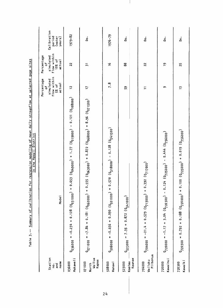
Tabl
e 3* Summary
of calibration
for
regr
essi
on modeling of mean da
ily
stre
amfl
ow at
se
lect
ed ga
ge sites
Sta
tion
no.
and
nam
e
0360
00
...
. ,.
^036
000
~ -"-^
Mak
awel
i
0710
00
_,.
...
^07
10
00
=
~7'°
4 N
ort
hW
a i 1
ua
Kap
aa
5080
00
, ,
U50
8000
=
-°-
b5b
H
anaw
i
5230
00
Q -
7 35
+
Kn
ola
u
^52
30
00
''*
+
Kea
nae
70^0
00
o k
,, .,
,
Q70
4000
=
~21
'4
Wa
t lu
ku
Pi
iho
nu
a
7200
00 . .
Q72
00
00
=
~''
17
Kaw
a t n
ut
7203
00
Q -
0 79
2 ..
. ^7
20
30
0
U'/
y^
Ka
wa
iki
in
the
H
aw
aii
Dis
tric
t
Perc
enta
ge
Pe
rce
nta
ge
o
f o
f sim
ula
ted
sim
ula
ted
Calibra
tion
flow
w
ith
in
flow
w
ithin
period
5% o
f 10
$ o
f (w
ate
r M
odel
a
ctu
al
actu
al
ye
ars
)
+ 0.1
28
3100
0)
+ 0.6
53
(QoA
900
o>
+ 1'7
7 ^0
19
00
0>
'
°'
121
^108000
) 12
22
19
79'8
2
+ °'
181
(%6
00
00
>
+ °-
555
(Q06
3000
>
+ °'8
72
(Q06
8000
) +
8-9
6 (Q
0715
00)
17
31
Do'
+ 0.
090
(Q50
1000
) +
0.57
0 (Q
5l8o
oo)
- 0.
128
(Q5/
j150
0)
7.8
16
19
76-7
9
°-87
2 (Q
5410
00>
59
88
Do'
+ 0.
579
(Q71
3000
) +
0.39
2 (Q
7170
00)
11
22
Do.
*o
n/iff
i \nio
li^n
^ n
/i li/
i ^ n
\
Q 10
n^
\ +
^.U
H
V^7
2Q30
0;
U'
I/H
11
472
50
00
; U
'HH
H
v^7
56
00
0;
y Iy
uo
*
+ oi8
8fo
^
+ o
inn
fo
^ +
oo
i^fo
^
1 n
2*1
DOT^
\j m
\ \
j\j
\ \j ~
j o ft
ft ft f
t /
* w
»iu
u
i ^C
T o
^n
nn
/ *
u
u
i j
\ w
r £
r\ r
\r\
/ * J
*-
J
v\j
/
jcU
U U
U
/ <L
j U
U U
/
jO U
U U
daily mean discharges at Waialae (019000), Waimea (031000), Hanapepe (049000),
and Wainiha (108000) were used as the explanatory variables.
The North Wailua Kapaa (071000) simulated data were within 10 percent of the
actual record only 31 percent of the time during the calibration period. These
results occurred when daily mean discharges at South Wailua (060000), North
Wailua Lihue (063000), East Wailua (068000) and Opaekaa (071500) were used as the
explanatory variables. The greatest hindrance to obtaining a satisfactory
simulation in this case was that the station was regressed against stations
having different flow characteristics at low flows. There is apparent seepage
loss between upstream stations and 071000.
The Hanawi (508000) simulated data were within 10 percent of the actual
record only 16 percent of the time during the calibration period. These results
occurred when daily mean discharges at Palikea (501000), Wailuaiki (518000) and
Manuel (541500) were used as the explanatory variables.
The most successful simulation of flow records was at Koolau Keanae (523000)
which was produced from regression with another station on the same ditch. The
dependent flow records were regressed against downstream ditch records for
Koolau Haipuaena (541000). The simulated data were within 10 percent for 88
percent of the calibration period and within 5 percent for 59 percent of the same
period. However, verification of the model using different period of data showed
that estimated data are considerably less accurate than that of the calibration
period. The estimated data were within 10 percent for 66 percent of the
verification period and within 5 percent for 34 percent of the same period.
Further improvement in the simulation was attempted by using two separate
models, one for high flows (Q >_ 30 ft /s at Koolau Haipuaena) and one for low
flows (Q < 30 ft /s at Koolau Haipuaena). Using the high- and low-flow models
did not improve the simulation. The overall simulation for Koolau Keanae
(523000), using the two models, reproduced the actual Koolau Keanae record within
10 percent for 84 percent of the calibration period and within 5 percent for 51
percent of the period.
The Wailuku Piihonua (704000) simulated data were within 10 percent of the
actual record only 22 percent of the time during the calibration period. These
results occurred when daily mean discharges at Wailuku Hilo (713000) and Honoli i
(717000) were used as the explanatory variables.
25
The Kawainui (720000) simulated data were
record only 19 percent of the time during the ca
occurred when daily mean discharges at Kawaiki
Kohakohau (756000) were used as the explanatory
The streamflow record for Kawaiki (720300)
within 10 percent of the actual
libration period. These results
(720300), Alakahi (725000) and
var iables.
was simulated with a regression
model that includes as explanatory variables, the streamflow at Kawainui
(720000), streamflow at Alakahi (725000), and streamflow at Kohakohau (756000).
Drainage basins for stations 720000, 720300 anc 756000 are located adjacent to
each other.
The simulated data for Kawaiki (720300) were within 10 percent of the actual
flows for 25 percent of the calibration period and within 5 percent for 13
percent of the period.
Some of the causes for low transferabi1ity
in the Hawaii District can be attributable to the small drainage areas causing
high-flow variability, variability of rainfall d
and local differences in basin cover and subsurface materials.
Conclusions Pertaining to Alternative Methods of Data Generation
of flow data among stream gages
istribution among nearby basins,
The simulated data from the regression me
were not sufficiently accurate to apply this
continuous-flow stream gage. It is suggested
operation as part of the Hawaii District stream
will be included in the next step of this analy;>
hod for the seven stream gages
method in lieu of operating a
that all seven stations remain in
gaging program; therefore, they
i s.
26
COST-EFFECTIVE RESOURCE ALLOCATION
Introduction to Kalman-Fi1tering for Cost-Effective
Resource Allocation (K-CERA)
In a study of the cost-effectiveness of a network of stream gages operated
to determine water consumption in the Lower Colorado River Basin, a set of
techniques called K-CERA were developed (Moss and Gilroy, 1980). Because of the
water-balance nature of that study, the measure of effectiveness of the network
was chosen to be the minimization of the sum of variances of errors of estimation
of annual mean discharges at each site in the network. This measure of effec
tiveness tends to concentrate stream-gaging resources on the larger, less stable
streams where potential errors are greatest. While such a tendency is appro
priate for a water-balance network, in the broader context of the multitude of
uses of the streamflow data collected in the USGS's Streamflow Information Pro
gram, this tendency causes undue concentration on larger streams. Therefore, the
original version of K-CERA was extended to include as optional measures of
effectiveness the sums of the variances of errors of estimation of the following
streamflow variables: annual mean discharge in cubic feet per second, annual
mean discharge in percentage, average instantaneous discharge in cubic feet per
second, or average instantaneous discharge in percentage. The use of percentage
errors does not unduly weight activities at large streams to the detriment of
records on small streams. In addition, the instantaneous discharge is the basic
variable from which all other streamflow data are derived. For these reasons,
this study used the K-CERA techniques with the sums of the variances of the
percentage errors of the instantaneous discharges at all continuously gaged
sites as the measure of the effectiveness of the data-collection activity.
The original version of K-CERA also did not account for error contributed by
missing stage or other correlative data that are used to compute streamflow data.
The probabilities of missing correlative data increase as the period between
service visits to a stream gage increases. A procedure for dealing with the
missing record has been developed and was incorporated into this study.
27
Brief descriptions of the mathematical p
effectiveness of the data-collection activity and
filtering (Gelb, 197^) to the determination of t
record are presented below. For more detail
applications of K-CERA, see Moss and Gilroy (1980)
Fontaine and others (1984).
Description of Mathematics
The program, called "The Traveling Hydrog
among stream gages a predefined budget for the cc
such a manner that the field operation is the mos
measure of effectiveness is discussed above. Th<
the manager is the frequency of use (number of tim
of routes that may be used to service the stre;
measurements. The range of options within the
daily usage for each route. A route is defined
gages and the least cost travel that takes the
operations to each of the gages and back to base,
with it an average cost of travel and average cost
visited along the way. The first step in this pa
the set of practical routes. This set of routes f
to an individual stream gage with that gage as
home base so that the individual needs of a str
isolation from the other gages.
Another step in this part of the analysis
special requirements for visits to each of the gag
periodic maintenance, rejuvenation of recording
sampling of water-quality data. Such special
inviolable constraints in terms of the minimum
requ
The final step is to use all of the above to
N., that the i.th route for i = 1,2, ..., NR, wher
routes, is used during a year such that (1) the
exceeded, (2) the minimum number of visits to eac
total uncertainty in the network is minimized. F
the form of a mathematical program. Figure 3 pr
28
ogram used to optimize cost-
of the application of Kalman
e accuracy of a stream-gaging
on either the theory or the
, Gilroy and Moss (1981), and
Program
rapher," attempts to allocate
1 lection of streamflow data in
cost-effective possible. The
set of decisions available to
s per year) of each of a number
m gages and to make discharge
program is from zero usage to
as a set of one or more stream
nydrographer from his base of
A route will have associated
of servicing each stream gage
rt of the analysis is to define
equently will contain the path
the lone stop and return to the
earn gage can be considered in
is the determination of any
55 for such things as necessary
quipment, or required periodic
irements are considered to be
number of visits to each gage,
determine the number of times,
i NR is the number of practical
budget for the network is not
h station is made, and (3) the
gure 2 represents this step in
;sents a tabular layout of the
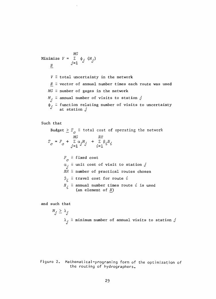
MGMinimize V = I d) . (M .)
7=1 J J
F = total uncertainty in the network
N_ = vector of annual number times each route was used
MG =. number of gages in the network
M . = annual number of visits to station jV
(j) . E function relating number of visits to uncertainty at station j
Such that
Budget _> T = total cost of operating the networkC?
MG Nfi T = F + La.M. + I. .N.
F E fixed cost oa . = unit cost of visit to station jV
NR = number of practical routes chosen
3. = travel cost for route ii
N. = annual number times route -i is used 7
(an element of N)
and such that
M. > X. J - J
X . =. minimum number of annual visits to station j
Figure 2 0 Mathematical-programing form of the optimization of the routing of hydrographers.
29
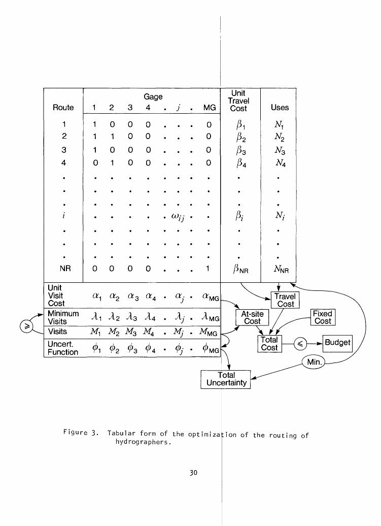
Route
12
3
4
NR
Unit Visit CostMinimum VisitsVisits
Uncert. Function
Gage1 MG
1 01 1
1 0
0 1
. .
. .
0
0
0
0
0
0
0
0
0
0
0
0
.. j...
0 0 0 0
I AM2 M3 . MMG
01 02 03 04 0; 01
UnitTravelCost
0
Uses
N, U
N
Figure 3- Tabular form of the optimization of the routing of hydrographers.
30
problem. Each of the NR routes is represented by a row of the table and each of
the stations is represented by a column. The zero-one matrix, (co. .)> defines the
routes in terms of the stations that comprise it. A value of one in row i and
column j indicates that gaging station j will be visited on route i; a value of
zero indicates that it will not. The unit travel costs, $., are the per-trip
costs of the hydrographer's travel time and any related per diem and operation,
maintenance, and rental costs of vehicles. The sum of the products of 3. and N.
for i = 1,2, ..., NR is the total travel cost assoc iated wi th the set of decisions
N = (N lf N 2 , ..., N NR ).
The unit-visit cost, a., is comprised of the average service and maintenance
costs incurred on a visit to the station plus the average cost of making a
discharge measurement. The set of minimum visit constraints is denoted by the
row A., j = 1,2, ..., MG, where MG is the number of stream gages. The row of
integers M., j = 1,2, ..., MG specifies the number of visits to each station. M.J -J
is the sum of the products of co.. and N. for all i and must equal or exceed X.
for all a. if j^ is to be a feasible solution to the decision problem.J
The total cost expended at the stations is equal to the sum of the products
of a. and M. for all j. The cost of record computation, documentation, and
publication is assumed to be influenced negl igibly by the number of visits to the
station and is included along with overhead in the fixed cost of operating the
network. The total cost of operating the network equals the sum of the travel
costs, the at-site costs, and the fixed cost, and must be less than or equal to
the available budget.
The total uncertainty in the estimates of discharges at the MG stations is
determined by summing the uncertainty functions, cj)., evaluated at the value of M.
from the row above it, for j = 1,2, ..., MG.
As pointed out in Moss and Gilroy (1980), the steepest descent search used
to solve this mathematical program does not guarantee a true optimum solution.
However, the locally optimum set of values for N^ obtained with this technique
specify an efficient strategy for operating the network, which may be the true
optimum strategy. The true optimum cannot be guaranteed without testing all
undominated, feasible strategies.
31
Description of Uncertainty
As noted earlier, uncertainty in streamf
study as the average relative variance of estimation of instantaneous
discharges. The accuracy of a streamflow estimate depends on how that estimate
was obtained. Three situations are considered
estimated from measured discharge and correlati
relation (rating curve), (2) the streamflow
secondary data at nearby stations because prima
Functions
ow records is measured in this
n this study: (1) streamflow is
ve data using a stage-discharge
record is reconstructed using
ry correlative data are missing,
and (3) primary and secondary data are unavailable for estimating streamflow.
The variances of the errors of the estimates of flow that would be employed in
each situation were weighted by the fraction of time each situation is expected
to occur. Thus, the average relative variance would be
wi th
where
V = £ r Vr + e V + £ f f r r e
1 = £ £ + £ + £ f r e
V is the average relative variance of the
e is the fraction of time that the primar
V- is the relative variance of the errors
recorders,
£ is the fraction of time that secondary d
streamflow records given that the pri
V is the relative variance of the error
structed from secondary data,
£ is the fraction of time that primary and
to compute streamflow records, and
V is the relative error variance of the t
The fractions of time that each source of
the frequencies at which the recording equipmen
32
(3)
errors of streamflow estimates,
recorders are functioning,
of flow estimates from primary
ita are available to reconstruct
irnary data are missing,
of estimation of flows recon-
secondary data are not available
ird situation.
error is relevant are functions of
is serviced.
The time, T, since the last service visit until failure of the recorder or
recorders at the primary site is assumed to have a negative-exponential
probability distribution truncated at the next service time; the distribution's
probability density function is
ft \ i kT// 1 ks\ MI \ f(i) = ke /(1-e ) (4)
where
k is the failure rate in units of (day)"" ,
e is the base of natural logarithms, and
s is the interval between visits to the site in days.
It is assumed that if a recorder fails it continues to malfunction until the next
service visit. As a result,
£f = ( 1 .e - ks )/( ks ) (5)
(Fontaine and others, 1984, eq. 21).
The fraction of time e that no records exist at either the primary or
secondary site can also be derived assuming that the time between failures at
both sites are independent and have negative exponential distributions with the
same rate constant. It then follows that,
£ e = 1 - [2(l-e"ks ) + 0.50-e-2ks )]/(ks)
(Fontaine and others, 1984, eqs. 23 and 25).
Finally, the fraction of time e that records are reconstructed based on
data from a secondary site is determined by the equation,
e = 1 - e r f
0.50-e-2ks )]/(ks)
33
The relative variance, V,., of the error derived from primary record computa
tion is determined by analyzing a time series of residuals that are the differ
ences between the logarithms of measured discharge and the rating curve
discharge. The rating curve discharge is determined from a relationship between
discharge and some correlative data such as water-surface elevation at the
gaging station. The measured discharge is the
observations of depths, widths, and velocities.
instantaneous discharge at time t and let qR (t
estimated using the rating curve. Then,
x(t) = 1n qT (t) - 1n q R (t) = 1n [C T (t)/qR (t)]
discharge determined by field
Let q T (t) be the true
) be the value that would be
(7)
iis the instantaneous difference between the logarithms of the true discharge and
the rating curve discharge.
In computing estimates of streamflow, the rating curve may be continually
adjusted on the basis of periodic measurements of discharge. This adjustment
process results in an estimate, q (t), that is a better estimate of the stream's
discharge at time t. The difference between the Variable x(t), which is defined
x(t) = 1n q c (t) - 1n q R (t)
and x(t) is the error in the streamflow record at
difference over time is the desired estimate of
Unfortunately, the true instantaneous di
mined and thus x(t) and the difference, x(t) -
well. However, the statistical properties of x
variance, can be inferred from the available di
observed residuals of measured discharge from the
z(t) = x(t) + v(t) = 1n q (t)m
where
(8)
time t. The variance of this
scharge, qT (t), cannot be deter-
(t), cannot be determined as
(t) - x(t), particularly, its
scharge measurements. Let the
rating curve be z(t) so that
- 1n q D (t) (9)
v(t) is the measurement error, and
1n q (t) is the logarithm of the measured d
to 1n qy (t) plus v(t).
ischarge equal
In the Kalman-fi1ter analysis, the z( t) time series was analyzed to
determine three site-specific parameters. The Kalman filter used in this study
assumes that the time residuals x(t) arise from a continuous first-order
Markovian process that has a Gaussian (normal) probability distribution with
zero mean and variance (subsequently referred to as process variance) equal to p.
A second important parameter is 3, the reciprocal of the correlation time of the
Markovian process giving rise to x(t); the correlation between x(t ) and x(t2 ) is
expf-Blt.-tp ]. Fontaine and others (1984) also define q, the constant value of
the spectral density function of the white noise which drives the Gauss-Markov
x-process. The parameters, p, q, and 3 are related by
Var[x(t)] = p = q/(23) (10)
The variance of the observed residuals z(t) is
Var[z(t)] = p + r (11)
where r is the variance of the measurement error v(t). The three parameters, p,
3, and r, are computed by analyzing the statistical properties of the z(t) time
series. These three site-specific parameters are needed to define this component
of the uncertainty relationship. The Kalman filter utilizes these three para
meters to determine the average relative variance of the errors of estimation of
discharge as a function of the number of discharge measurements per year (Moss
and Gilroy, 1980).
If the recorder at the primary site fails and there are no concurrent data
at other sites that can be used to reconstruct the missing record at the primary
site, there are at least two ways of estimating discharges at the primary site.
A recession curve could be applied from the time of recorder stoppage until the
gage was once again functioning, or the expected value of discharge for the
period of missing data could be used as an estimate. The expected-value approach
is used in this study to estimate V , the relative error variance during periodsC
of no concurrent data at nearby stations. If the expected value is used to
estimate discharge, the value that is used should be the expected value of
discharge at the time of year of the missing record because of the seasonal i ty of
the streamflow processes. The variance of streamflow, which also is a sea
sonally varying parameter, is an estimate of the error variance that results from
35
using the expected value as an estimate. Thus, the coefficient of variation
squared (C ) is an estimate of the required relative error variance V . Because
C varies seasonally and the times of failures cannot be anticipated, a
seasonally averaged value of C is used:
where
a.
c =v
1355
365 a
is the standard deviation of daily di
year,
is the expected value of discharge on the i day of the year, and
2 .
(100) (12)
scharges for the i day of the
.th
is used as an estimate of V .e
The variance, V , of the relative error during periods of reconstructed
streamflow records is estimated on the basis of
the primary site and records from other gaged
correlation between records at
nearby sites. The correlation
coefficient, p , between the streamflows with seasonal trends removed at the site
of interest and detrended streamflows at the other sites is a measure of the
goodness of their linear relationship. The fraction of the variance of stream-
flow at the primary site that is explained by data from the other sites is equal2 to p . Thus, the relative error variance of flow estimates at the primary site
obtained from secondary information will be
V = (1-p 2 ) C 2 r c v (13)
Sometimes the record for a gaging station can be reconstructed by correla
tion with more than one nearby gaging station. F : or the fraction of time when no
secondary data are available from the gaging station typically used (secondary
station) for record reconstruction (e ), data from another (tertiary) gaging
station can be used. The correlation of data from the tertiary station with data
from the station of interest is denoted R, The
or equal to p . The variance of records estimated from a tertiary source of
information is
(1 - R*) (Cy ) 2 = (1 - R*) Ve .
value of R« is always less than
36
Because errors in streamflow estimates arise from three different sources
with widely varying precisions, the resultant distribution of those errors may
differ significantly from a normal or log-normal distribution. This lack of
normality causes difficulty in Interpretation of the resulting average estima
tion variance. When primary and secondary data are unavailable, the relative
error variance V may be very large. This could yield correspondingly large
values of V in equation (3) even if the probability that primary and secondary
information are not available, e , is quite small.
A new parameter, the equivalent Gaussian spread (EGS), is introduced here to
assist in interpreting the results of the analyses. If it is assumed that the
various errors arising from the three situations represented in equation (3) are
log-normally distributed, the value of EGS was determined by the probability
statement that
Probability [e" EGS < (q c (t) / q T (t)) < e+EGS ] = 0.683 (14)
2 Thus, if the residuals In q (t) - 1n q-r(t) were normally distributed, (EGS)
would be their variance. Here EGS is reported in units of percent because EGS is
defined so that nearly two-thirds of the errors in instantaneous streamflow data
will be within plus or minus EGS percent of the reported values.
The Application of K-CERA in the Hawaii District
As a result of the first two parts of this analysis, it has been suggested
that all 124 of the currently existing stream gages in the Hawaii District
program be continued in operation. These 124 stream gages were subjected to the
K-CERA analysis with results that are described below.
Definition of Missing Record Probabilities
As described earlier, the statistical characteristics of missing stage or
other correlative data for computation of streamflow records can be defined by a
single parameter, the value of k in the truncated negative exponential probabi
lity distribution of times to failure of the equipment. In the representation of
f(i) as given in equation 4, the average time to failure is 1/k. The value of 1/k
37
will vary from site to site depending upon the type of equipment at the site and
upon its exposure to natural elements and vanda
changed by advances in the technology of data
estimate 1/k in the Hawaii District, a period of actual data collection of 7
years duration in which little change in technology occurred and in which stream
gages were visited on a consistent pattern o
estimates of 1/k were determined for different geographical areas of the
District. During this 7-year period one estimate
in the State of Hawaii, was based on an average
could be expected to be malfunctioning and 8 vis
Another estimate of 1/k (370 days), for stations in American Samoa, was
based on an average of ^ percent of the time a
malfunctioning and 12 visits per year. The third
ism. The value of 1/k can be
collection and recording. To
frequency was used. Three
of 1/k (555 days), for stations
of ^ percent of the time a gage
its per year.
gage could be expected to be
estimate of 1/k (180 days), for
stations in the Other Pacific Areas other than in American Samoa, was based on an
average of 8 percent of the time a gage could be expected to be malfunctioning
and 12 visits per year. The appropriate 1/k estimate for each geographical area
was used to determine e, and e , for each of the 12^ stream gages as a
function of the individual frequencies of visit.
Definition of Cross-Correlation
Coefficient of Varia
Coefficient and
ion
To compute the values of V and V of the: needed uncertainty functions,
daily streamflow records for each of the 12^ steitions for the last 30 years or
the part of the last 30 years for which daily :;treamflow values are stored in
WATSTORE (Hutchinson, 1975) were retrieved. For' each of the stream gages that
had 3 or more complete water years of data, the value of C was computed and
various options, based on combinations of other stream gages, were explored to
determine the maximum p For the three stati ons that had less than 3 water
sted in table
years of data, values of C and p were estimated subjectively
The set of parameters for each station and
the highest cross correlation coefficient are 1
fact from this step of the study is that two stat
although the correlation is poor, with stations
other. This could be due just to chance.
the auxiliary records that gave
A surprising
ions on Saipan correlate better,
on Guam than they do with each
38
Table 4. Statistics of record reconstruction
Station no.
010000019000031000036000049000
060000061000061200062000063000
068000069000071000071500077000
079000080000087000088000089000
091000097500100000103000108000
200000208000211600212800213000
216000226000229000229300232000
240500254000272200283600283700
CV
159181215177174
19422.623.3
172134
11789.313611088.6
114205181127172
13510564.6123113
159160174197137
231263172166144
10412380.149.037.7
p c
0.784.895.856.941.915
.930
.632
.717
.483
.929
.935
.422
.966
.774
.496
.354
.898
.712
.586
.867
.445
.894
.530
.837
.884
.859
.886
.591
.892
.839
.853
.906
.940
.897
.835
.832
.830
.758
.939
.939
R2
0.709.709.456.727.680
.900
.388
.700
.096
.868
.900
.366
.904
.700
.168
.192
.800
.700
.486
.800
.340
.800
.500
.800
.800
.756
.772
.475
.799
.671
.779
.811
.820
.766
.756
.752
.638
.587
.294
.312
Source of
031000031000010000031000031000
049000061200061000061000069000
060000063000060000068000079000
069000068000088000087000068000
077000080000062000036000036000
212800200000213000200000208000
226000216000226000229000229000
226000229000229000283700283600
reconstructed
108000108000019000049000036000
063000
062000063000071000
063000068000063000080000088000
077000089000089000089000080000
087000089000063000108000103000
208000212800216000208000216000
229000229000229300240500240500
229000272200229300284200284200
records
036000108000
071000
063000100000
080000071000068000089000
080000
091000091000097500
088000103000103000
345000345000345000345000345000
229300229300240500
229300240500254000294900294900
See footnote at end of table, p. 42.39
Table 4. Statistics of record reconstruction Cent inued
Station no.
284200 294900 296500 302000 303000
304200 325000 330000 345000 400000
404200405100405300405500408000
414000419500501000508000512000
518000523000531000538000541000
541500587000588000589000592000
594000599500618000620000638500
700000700900700950*704000713000
CV
62.2 146 116 91.6 118
166173 214 175 149
78.210259.7
171116
13620021819165.3
19060.712995.465.9
20213649.117792.1
18488.8129108157
91.883.580188131
p c
0.693 .834 .804 .407 .765
.808
.921 907 .880 .698
.746
.959
.959
.870
.901
.685
.724
.688
.970
.947
.967
.985 729.864.984
.882
.802
.896
.826
.789
.760
.788
.839
.880
.539
.825 796.80.872.810
R2
0.143 .593 .712 .054 .600
.659
.749
.793
.793
.626
.700
.462
.433
.655
.745
.636
.574
.562
.846
.827
.739
.942
.648
.847
.943
.846
.762
.874
.766
.722
.680
.757
.689
.739
.385
.465
.489
.50
.727
.727
Source of
2836 2836 200C 303C 3020
325C 330C 325C 208C 4055
4055405;405140424042
4042400C508C501C523C
508C512C512C512C512(
508(508(512(
00 00 00 00 00
00 00 00 00 00
;oo00000000
0000000000
0000000000
IOOtoo00
538000541000
512000512(518(508(518(
700<700(
00000000
0000
713000704000
reconstructed records
283700 284200 208000 325000 325000
345000 345000 345000 325000 408000
408000405500405500408000405500
405500404200518000518000538000
541500541000538000523000523000
518000518000523000541000588000
538000523000541500518000587000
713000713000
717000717000
294900 296500 345000
345000
304200 304200
330000 419500
408000408000541500541500541000
620000588000541000541000538000
620000620000541000592000589000
589000541000620000618000620000
See footnote at end of table, p. 42.40
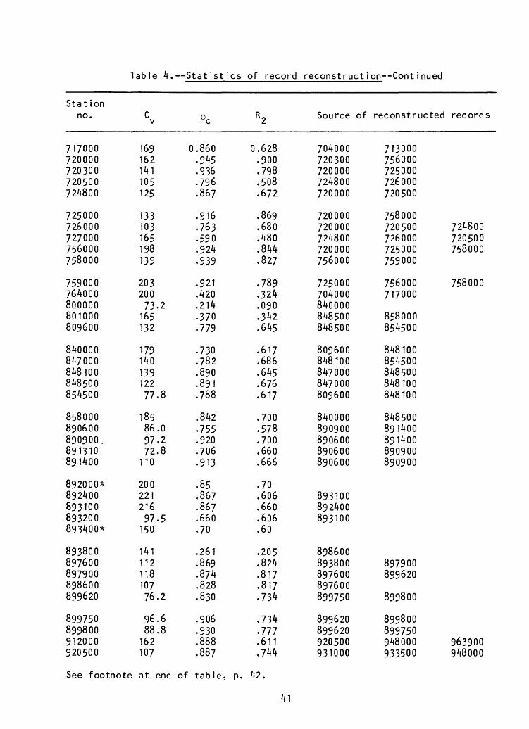
Table 4. Statistics of record reconstruction--Continued
Stat ion no.
717000720000720300720500724800
725000726000727000756000758000
759000764000800000801000809600
840000847000848100848500854500
858000890600890900.891310891400
892000*892400893100893200893400*
893800897600897900898600899620
899750899800912000920500
CV
169162141105125
133103165198139
20320073.2165132
17914013912277.8
18586.097.272.8110
20022121697.5150
14111211810776.2
96.688.8162107
PC
0.860.945.936.796.867
.916
.763
.590
.924
.939
.921
.420
.214
.370
.779
.730
.782
.890
.891
.788
.842
.755
.920
.706
.913
.85
.867
.867
.660
.70
.261
.869
.874
.828
.830
.906
.930
.888
.887
R2
0.628.900.798.508.672
.869
.680
.480
.844
.827
.789
.324
.090
.342
.645
.617
.686
.645
.676
.617
.700
.578
.700
.660
.666
.70
.606
.660
.606
.60
.205
.824
.817
.817
.734
.734
.777
.611
.744
Source of
704000720300720000724800720000
720000720000724800720000756000
725000704000840000848500848500
809600848100847000847000809600
840000890900890600890600890600
893100892400893100
898600893800897600897600899750
899620899620920500931000
reconstructed
713000756000725000726000720500
758000720500726000725000759000
756000717000
858000854500
848100854500848500848100848100
848500891400891400890900890900
897900899620
899800
899800899750948000933500
records
724800720500758000
758000
963900948000
See footnote at end of table, p. 42.
41
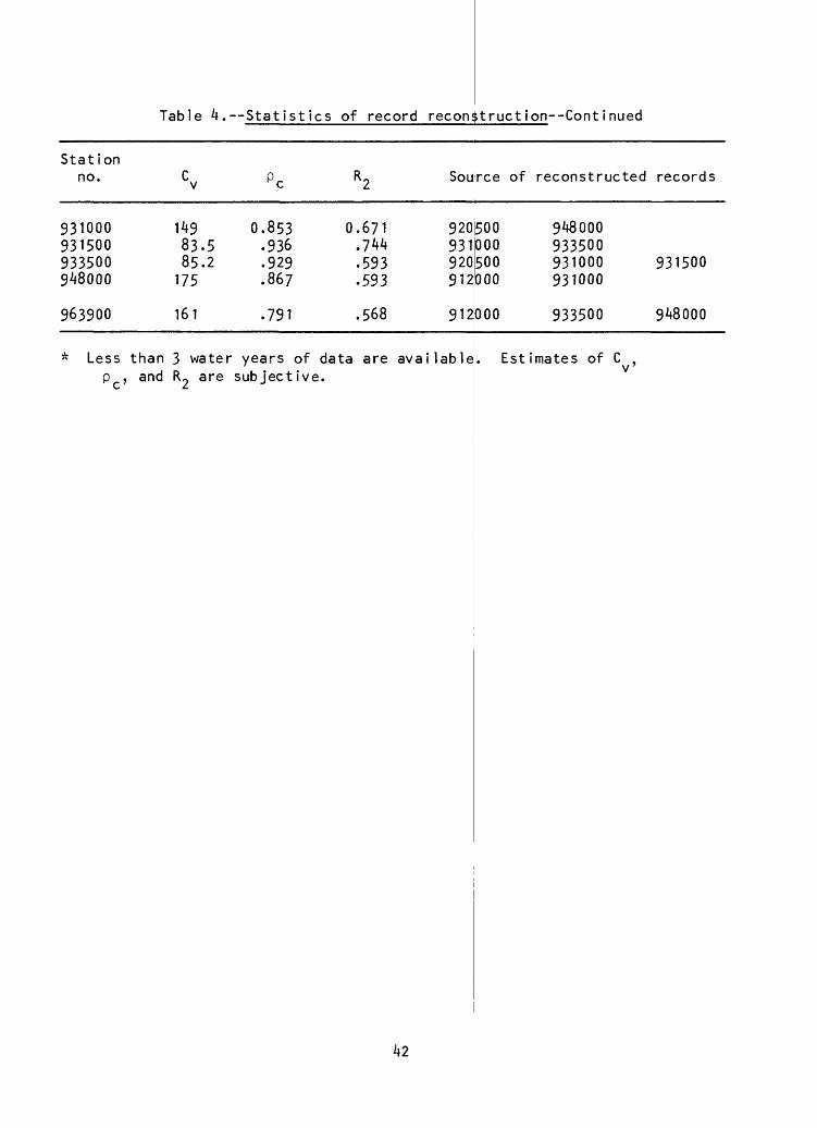
Table 4. Statistics of record reconstruct I on--Continued
Station no.
931000 931500 933500 948000
963900
* Less than P c > and
CV
149 83.5 85.2175
161
3 wa te r R~ are
p c
0.853 o.936 .929 .867
.791
years of data subjective.
«2
.671
.744
.593
.593
.568
are
Source
920931 920 912
912
avai lable
500 000 500 000
000
of reconstructed
948000 933500 931000 931000
933500
records
931500
948000
Estimates of C , v'
42
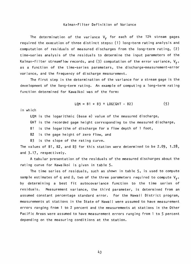
Kalman-Fi1ter Definition of Variance
The determination of the variance V,. for each of the 124 stream gages
required the execution of three distinct steps: (1) long-term rating analysis and
computation of residuals of measured discharges from the long-term rating, (2)
time-series analysis of the residuals to determine the input parameters of the
Kalman-fi1ter streamflow records, and (3) computation of the error variance, V.p,
as a function of the time-series parameters, the discharge-measurement-error
variance, and the frequency of discharge measurement.
The first step in the determination of the variance for a stream gage is the
development of the long-term rating. An example of computing a long-term rating
function determined for Kawaikoi was of the form:
LQM = B1 + B3 * LOG(GHT - B2) (5)
in which
LQM is the logarithmic (base e) value of the measured discharge,
GHT is the recorded gage height corresponding to the measured discharge,
B1 is the logarithm of discharge for a flow depth of 1 foot,
B2 is the gage height of zero flow, and
B3 is the slope of the rating curve.
The values of B1, B2, and B3 for this station were determined to be 2.09, 1.28,
and 3.17, respectively.
A tabular presentation of the residuals of the measured discharges about the
rating curve for Kawaikoi is given in table 5.
The time series of residuals, such as shown in table 5> is used to compute
sample estimates of q and 3, two of the three parameters required to compute V,.,
by determining a best fit autocovar iance function to the time series of
residuals. Measurement variance, the third parameter, is determined from an
assumed constant percentage standard error. For the Hawaii District program,
measurements at stations in the State of Hawaii were assumed to have measurement
errors ranging from 1 to 2 percent and the measurements at stations in the Other
Pacific Areas were assumed to have measurement errors ranging from 1 to 5 percent
depending on the measuring conditions at the station.
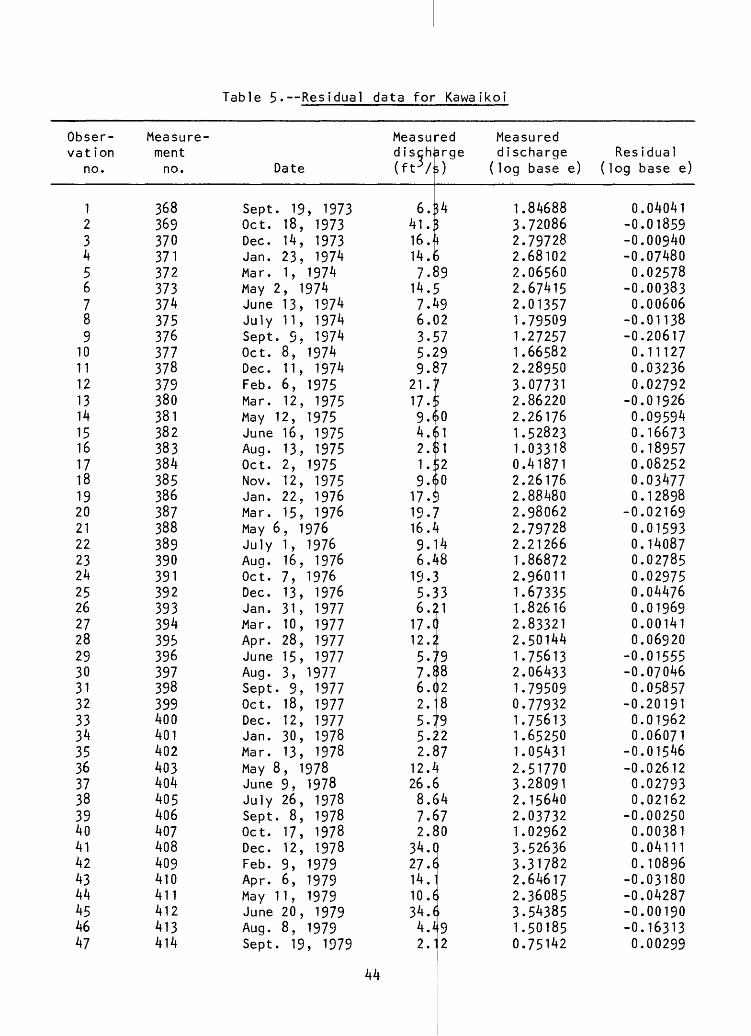
Table 5- Residual data for Kawaikoi
Obser vation
no.
123456789
1011121314151617181920212223242526272829303132333435363738394041424344454647
Measure ment no.
368369370371372373374375376377378379380381382383384385386387388389390391392393394395396397398399400401402403404405406407408409410411412413414
Date
Sept. 19, 1973Oct. 18, 1973Dec. 14, 1973Jan. 23, 1974Mar. 1, 1974May 2, 1974June 13, 1974July 11, 1974Sept. 9, 1974Oct. 8, 1974Dec. 11, 1974Feb. 6, 1975Mar. 12, 1975May 12, 1975June 16, 1975Aug. 13, 1975Oct. 2, 1975Nov. 12, 1975Jan. 22, 1976Mar. 15, 1976May 6, 1976July 1, 1976Aug. 16, 1976Oct. 7, 1976Dec. 13, 1976Jan. 31, 1977Mar. 10, 1977Apr. 28, 1977June 15, 1977Aug. 3, 1977Sept. 9, 1977Oct. 18, 1977Dec. 12, 1977Jan. 30, 1978Mar. 13, 1978May 8, 1978June 9, 1978July 26, 1978Sept. 8, 1978Oct. 17, 1978Dec. 12, 1978Feb. 9, 1979Apr. 6, 1979May 11, 1979June 20, 1979Aug. 8, 1979Sept. 19, 1979
Measul disclr(ft 5 /:
6.:41.;16.'14.<7.1
14.;7. J6. 13.!5.:9J
21.;17.19.<
-ed arge0
54Ii>59?*9)2- >!
IS571 >>0
4.612.11.'9.<
17.!19.;16J9.6.1
19.:5.^6.217. C12.25o7.?6.C2. 15-y5.22.1
12.'26 A8.<7-t2.1
34. C27.*14.10 .d34. <4.'2.1
si520
4>8
13!1
'9!8128'9:2!7
,4>7;o
92
Measured discharge
( log base e)
1.846883.720862.797282.681022.065602.674152.013571.795091.272571.665822.289503.077312.862202.261761.528231.033180.418712.261762.884802.980622.797282.212661.868722.960111.673351.826162.833212.501441.756132.064331.795090.779321.756131.652501.054312.517703.280912.156402.037321.029623.526363.317822.646172.360853.543851.501850.75142
Res idual ( log base e)
0.04041-0.01859-0.00940-0.074800.02578
-0.003830.00606
-0.01138-0.206170.111270.032360.02792
-0.019260.095940.166730.189570.082520.034770.12898
-0.021690.015930.140870.027850.029750.044760.019690.001410.06920
-0.01555-0.070460.05857
-0.201910.019620.06071
-0.01546-0.026120.027930.02162
-0.002500.003810.041110.10896-0.03180-0.04287-0.00190-0.163130.00299
44
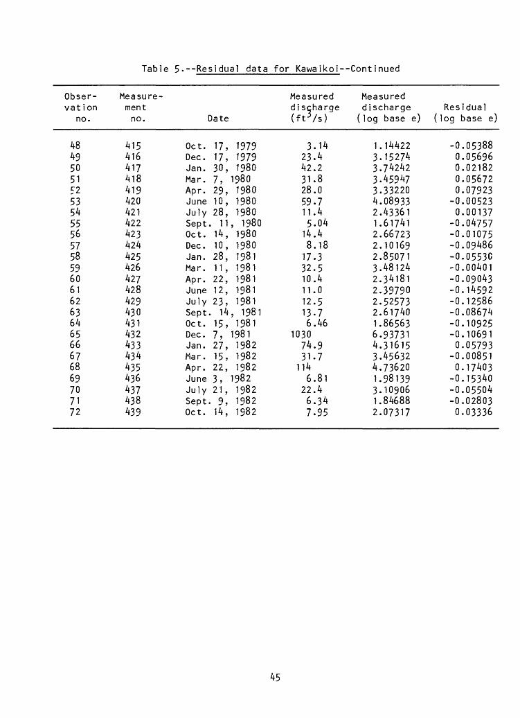
Table 5.--Residual data for Kawa}koi--Continued
Obser vation
no.
48495051525354555657585960616263646566676869707172
Measure ment no.
415416417418419420421422423424425426427428429430431432433434435436437438439
Date
Oct. 17, 1979Dec. 17, 1979Jan. 30, 1980Mar. 7, 1980Apr. 29, 1980June 10, 1980July 28, 1980Sept. 11, 1980Oct. 14, 1980Dec. 10, 1980Jan. 28, 1981Mar. 11, 1981Apr. 22, 1981June 12, 1981July 23, 1981Sept. 14, 1981Oct. 15, 1981Dec. 7, 1981Jan. 27, 1982Mar. 15. 1982Apr. 22, 1982June 3, 1982July 21, 1982Sept. 9, 1982Oct. 14, 1982
Measured discharge (ft 3 /s)
3.1423.442.231.828.059.711.45.04
14.48.1817.332.510.411.012.513.76.46
103074.931.7
1146.81
22.46.347.95
Measured discharge
( log base e)
1.144223.152743.742423.459473.332204.089332.433611.617412.667232.101692.850713.481242.341812.397902.525732.617401.865636.937314.316153.456324.736201.981393.109061.846882.07317
Residual ( log base e)
-0.053880.056960.021820.056720.07923
-0.005230.00137
-0.04757-0.01075-0.09486-0.05530-0.00401-0.09043-0.14592-0.12586-0.08674-0.10925-0.106910.05793
-0.008510.17403
-0.15340-0.05504-0.028030.03336
45
As discussed earlier, q and 3 can be expressed as the process variance of
the shifts from the rating curve and the 1-day
these shifts. Table 6 presents a summary of the autocovariance analysis
expressed in terms of process variance and 1-day outocorrelation for all stations
in the Di str ict.
The autocovariance parameters, summarized
definition of missing record probabilities, summarized in table 4, are used
jointly to define uncertainty functions for each
functions give the relationship of total error variance to the number of visits
and discharge measurements. An example of an uncertainty function is given in
figure 4. This function is based on the assumption that a measurement was made
during each visit to the station.
Stations 303000 and 899620 were assigned /:ero uncertainty because it was
assumed that the residual time series was not an auto-regressive process at these
autocorrelation coefficient of
in table 6, and data from the
gaging station. The uncertainty
stations. They were not included in the average
In the Hawaii District, feasible routes to service the 124 stream gages were
determined after consultation with personnel in
the Hawaii District office and after review of
standard error calculations.
the Hydrologic Data Section of
the uncertainty functions. The
gaging stations were divided into two groups. One group is for the State of
Hawaii stations and the second the Other Pacific Areas. In summary, 92 routes
were selected to service all the stream gages in
routes were selected for the Other Pacific Are;js. These routes included all
possible combinations that describe the current operating practice, alternatives
that were under consideration as future possibilities, routes that visited
certain key individual stations, and combinations that grouped proximate gages
where the levels of uncertainty indicated more frequent visits might be useful.
These routes and the stations visited on each are summarized in tables 7 and 8.
The costs associated with the practical routes must be determined. Fixed
costs to operate a gage typically include equipment rental, batteries, electric
ity, data processing and storage, computer charges, maintenance, miscellaneous
supplies, and analysis and supervisory charges.
values were applied to each station in the progrc
46
the State of Hawaii. Forty-one
-or the Hawaii District, average
m for all the above categories.
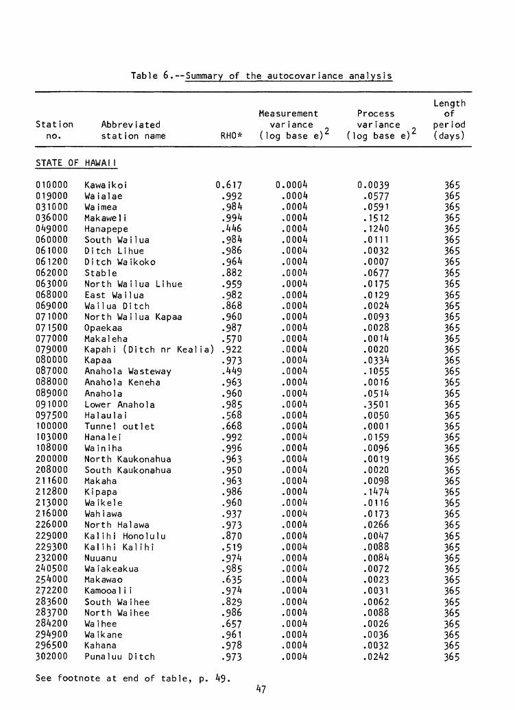
Table 6. Summary of the autocovariance analysis
Stat ion no.
Abbreviated station name RHO*
Measurement variance
( log base e)
Process variance
( log base e)
Length of
per iod (days)
STATE OF HAWAI 1
010000019000031000036000049000060000061000061200062000063000068000069000071000071500077000079000080000087000088000089000091000097500100000103000108000200000208000211600212800213000216000226000229000229300232000240500254000272200283600283700284200294900296500302000
Kawa ikoiWa ialaeWa i meaMakawel iHanapepeSouth Wa i 1 uaDitch LihueDitch WaikokoStableNorth Wa i 1 ua Li hueEast Wa i 1 uaWailua DitchNorth Wa i lua KapaaOpaekaaMakalehaKapahi (Ditch nr KealKapaaAnahola WastewayAnahola KenehaAnaholaLower AnaholaMalaula iTunnel outletHanaleiWa in ihaNorth KaukonahuaSouth KaukonahuaMakahaKipapaWa i k e 1 eWah iawaNorth HalawaKal i h i Honolu luKalihi KalihiNuuanuWa iakeakuaMakawaoKamooa 1 i iSouth WaiheeNorth WaiheeWa i heeWa ikaneKahanaPunaluu Ditch
0.617.992.984.994.446.984.986.964.882.959.982.868.960.987.570
ia) .922.973.449.963.960.985.568.668.992.996.963.950.963.986.960.937.973.870.519.974.985.635.974.829.986.657.961.978.973
0.0004.0004.0004.0004.0004.0004.0004.0004.0004.0004.0004.0004.0004.0004.0004.0004.0004.0004.0004.0004.0004.0004.0004.0004.0004.0004.0004.0004.0004.0004.0004.0004.0004.0004.0004.0004.0004.0004.0004.0004.0004.0004.0004.0004
0.0039.0577.0591.1512.1240.0111.0032.0007.0677.0175.0129.0024.0093.0028.0014.0020.0334.1055.0016.0514.3501.0050.0001.0159.0096.0019.0020.0098.1474.0116.0173.0266.0047.0088.0084.0072.0023.0031.0062.0088.0026.0036.0032.0242
365365365365365365365365365365365365365365365365365365365365365365365365365365365365365365365365365365365365365365365365365365365365
See footnote at end of table, p. 49.47
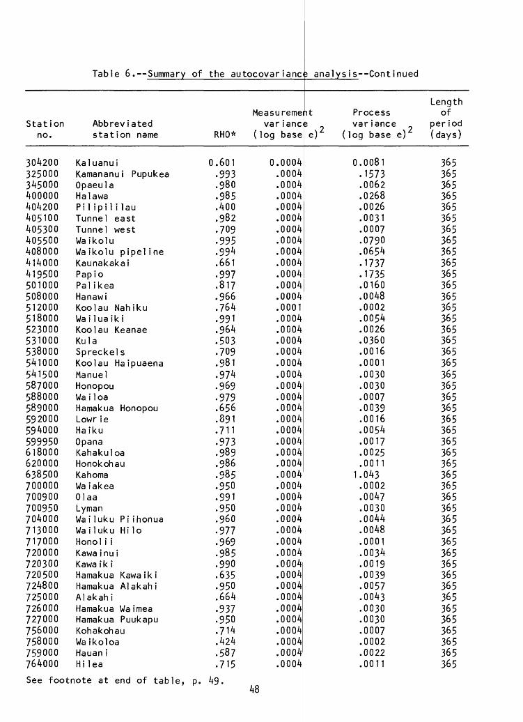
Table 6. Summary of the autocovar iance analysis Cent inued
Station no.
3042003250003450004000004042004051004053004055001*08000414000419500501000508000512000518000523000531000538000541000541500587000588000589000592000594000599950618000620000638500700000700900700950704000713000717000720000720300720500724800725000726000727000756000758000759000764000
Abbreviated station name
KaluanuiKamananui PupukeaOpaeulaHalawaPi 1 ipi 1 i lauTunnel eastTunnel westWa i k o 1 uWa ikolu pipel i neKaunakakaiPapioPal ikeaHanawiKoolau NahikuWa i lua ik iKoolau KeanaeKulaSpreckelsKoolau HaipuaenaManuelHonopouWa i 1 oaHamakua HonopouLowr ieHa ikuOpanaKahakuloaHonokohauKahomaWa iakeaOlaaLymanWa i luku Pi ihonuaWa i luku Hi loHonol i iKawa inu iKawa i k iHamakua KawaikiHamakua AlakahiAlakahiHamakua WaimeaHamakua PuukapuKohakohauWa i k o 1 oaHauan iHilea
See footnote at end of table,
RHO*
0.601.993.980.985.400.982.709.995.994.661.997.817.966.764.991.964.503.709.981.974.969.979.656.891.711.973.989.986.985.950.991.950.960.977.969.985.990.635.950.664.937.950.714.424.587.715
P. 49.
Measureme var ianc
( log base
0.0004.0004.0004.0004.0004.0004.0004.0004.0004.0004.0004.0004.0004.0001
it Process 2 variance e) ( log base e)
0.0081.1573.0062.0268.0026.0031.0007.0790.0654.1737.1735.0160.0048.0002
.0004 .0054
.0004 .0026
.0004 .0360
.0004
.0004
.0004
.0004
.0004
.0004
.0004
.0004
.0004
.0004
.0004
.0004
.0004
.0004
.0004
.0004
.0004
.0004
.0004
.0004
.0004
.0004
.0004
.0004
.0004
.0004
.0004
.0004
.0004
i r\
.0016
.0001
.0030
.0030
.0007
.0039
.0016
.0054
.0017
.0025
.00111.043.0002.0047.0030.0044.0048.0001.0034.0019.0039.0057.0043.0030.0030.0007.0002.0022.0011
Length of
per iod (days)
365365365365365365365365365365365365365365365365365365365365365365365365365365365365365365365365365365365365365365365365365365365365365365
48
Table 6. Summary of the autocovar iance analysis Cent inued
Station no.
Abbreviated station name
Measurement variance
RHO* (log base e) 2
Process variance
( log base e)
Length of
per iod (days)
OTHER PACIFIC AREAS
800000801000809600840000847000848100848500854500858000890600890900891400891310892000892400893100893200893400893800897600897900898600899750899800912000920500931000931500933500948000963900
Denn iTalofofoLa Sa FuaTinagaImongAlmagosaMau lapUgumYl igDiongradidTabeched ingNgerdorchKmekumelQatl iwQar ingeelBurongMukongEyebWichenNanpi 1LewiLuhpworMalemTofolPagoAasuAtaulomaAsil iLeafu LeoneAfueloLeafu Auasi
0.940.961.954.923.867.928.982.979.827.995.965.979.937 i;.950-'.912.939.939.916.950-y.973.934.331.986.912.901.954.977.746.930.801.985
0.0025.0025.0025.0016.0025.0025.0025.0025.0025.0025.0001.0025.0004.0025.0025.0004.0025.0025.0025.0025.0025.0025.0025.0025.0004.0004.0004.0004.0004.0004.0004
0.0590.2170.0466.0451.0462.0195.0151.0042.0240.0061.0022.0074.0041.0250.0555.0267.1607.1770.0371.0390.0346.0044.0624.0079.0128.0119.1156.0169.0121.0590.1669
365365365365365365365365365365365365365365365365365365365365365365365365365365365365365365365
* One-day autocorrelation coefficient.
Estimate.
49
200
un
O
ST
AT
ION
010000 (
KA
WA
IKO
I)
5
10
15
20
25
NU
MB
ER
O
F V
ISIT
S
AN
D
ME
AS
UR
EM
EN
TS
P
ER
Y
EA
R
Figure 4.
Typical
uncertainty
func
tion
fo
r in
stantaneous
discharge,
30
Table 1. Summary of the routes that may be used to visit
Route no.
123456789
10111213141516171819202122232k2526272829303132333435363738394041424344454647
010000019000031000036000060000061000061200068000071000071500077000080000097500103000010000060000062000069000071000080000087000089000097500100000200000208000211600212800213000226000229000229300240500254000272200283600294900302000330000345000325000216000304200200000211600212800212800
stat
108000
049000063000100000062000
079000087000
031000061000063000077000071500
088000091000103000
216000
232000
283700296500303000
208000213000226000345000
ions in the State of Hawaii
Stations serviced on the route
069000
088000089000 091000
061200068000079000
284200
304200
216000
51
Table 7«--Summary of the routes that: may be used to visit
Route no.
4849505152535^5556575859606162636465666768697071727374757677787980818283848586878889909192
226000325000232000325000400000419500405100414000404200400000414000405100501000508000512000531000538000587000588000592000618000620000638500531000541500589000594000620000508000538000501000700000700900700950704000713000717000720000726000764000727000700900700900713000720000
stat ions
229300330000254000330000
405300
419500419500405300
541500518000599500541000
589000594000
638500531000541000508000
720300727000
700950700950717000720300
in the State of Haw
Stations serviced c
232000
272200345000
405500 408000
405500 408000 l
523000
541500512000 518000 5
720500 724800 7756000 758000 7
704000
720500 724800 7
a i i--Cont inued
n the route
14000 419500
23000 541500
2500059000
25000 726000 727000 756000
52
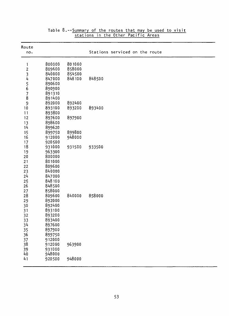
Table 8.--Summary of the routes that may be used to visit
Route no.
123456789
10111213141516171819202122232k2526272829303132333^35363738394041
80000080960084000084700089060089090089131089140089200089310089380089760089860089962089975091200092050093100096390080000080100080960084000084700084810084850085800080960089200089240089310089320089-3400897600897900899750912000912000931000948000920500
stations in the Other Pacific Areas
Stations serviced on the route
801000858000854500848100 848500
892400893200 893400
897900
899800948000
931500 933500
840000 858000
963900
948000
53
Visit costs are those associated with paying the hydrographer for the time
actually spent at a station servicing the equipment and making a discharge
measurement. These costs vary from station to station and are a function of the
difficulty and time required to make the discharge measurement. Average visit
times were calculated for each station base<! on an analysis of discharge
measurement data available. This time was then nultiplied by the average hourly
salary of hydrographers in the respective field offices of the Hawaii District to
determine total visit costs.
Route costs include the vehicle cost assoc
miles it takes to cover the route, the cost of
transit, and any per diem associated with the tim
ated with driving the number of
he hydrographer's time while in
e it takes to complete the trip.
K-CERA Results
The "Traveling Hydrographer Program" uti
along with the appropriate cost data and route
cost-effective way of operating the stream-gagi
the first step was to simulate the current
uncertainty associated with it. To accomplish
made to each stream gage and the specific rout
these visits were fixed. Current practice fo
discharge measurements to be made 100 percent
visited, except when there is no flow in the str
was observed, past measurement record was exami
of making a measurement at each such site and
resulting average error of estimation for the
Hawaii and the Other Pacific Areas is plotted as
21.0 percent and 25.9 percent, respectively.
The line labeled 'with lost record 1 on
minimum level of average uncertainty that can be
the existing instrumentation and technology,
runs of the "Traveling Hydrographer Program"
straints on the operations other than budget we
izes the uncertainty functions
definitions to compute the most
ng program. In this application,
practice and determine the total
his, the number of visits being
es that are being used to make
the Hawaii District calls for
of the time that a station is
earn. For stations where no flow
ned to determine the probability
adjustments were applied. The
current practice in the State of
a point in figures 5 and 6 and is
gures 5 and 6 represents the
ined for a given budget with
line was defined by several
different budgets. Con-
defined as described below.
i
obta "he
wi
e
th
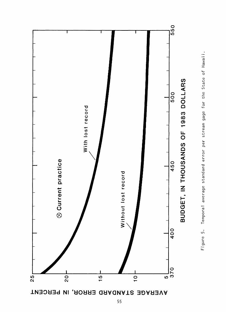
AVERAGE STANDARD ERROR, IN PERCENT
inc
-I CD 3-o o-\0)
CD-1
O)in
CD
15 CL O)T Q.
CD
CD O)3
to
CD
CO M-
O)
CD
o
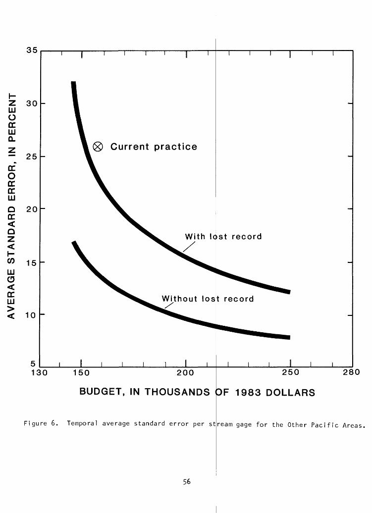
35
Z 30 LUO CC LU CL
- 25 t
CCoCC CC LLI
Q 20 CC < OZ
15LLI O
CC LLI
< 10
1 I T
Current practice
With lost record
Without lost record
I I 1130 150 200 250
BUDGET, IN THOUSANDS OF 1983 DOLLARS
Figure 6. Temporal average standard error per stream gage for the Other Pacific Areas
I I I i280
To determine the minimum number of times each station must be visited,
consideration was given to the physical limitations of the method used to record
data. The effect of visitation frequency on the accuracy of the data and amount
of lost record is taken into account in the uncertainty analysis. In the Hawaii
District, a minimum requirement of four visits per year was calculated and
applied to most stations. This value was based on limitations of the batteries
used to drive recording equipment, and the capacities of the uptake spools on the
digital recorders.
Minimum visit requirements should also reflect the need to visit stations
for special reasons such as water-quality sampling. In the Hawaii District,
water-quality work for the benchmark and NASQAN stations do influence minimum
visit requirements.
The results in figures 5 and 6, and tables 9 and 10 summarize the K-CERA
analysis. It should be emphasized that figures 5 and 6, and tables 9 and 10 are
based on various assumptions (stated previously) concerning both the time series
of shifts to the stage-discharge relationship and the methods of record recon
struction. Where a choice of assumptions was available, the assumption that
would not underestimate the magnitude of the error variances was chosen.
It can be seen that the current policy results in an average standard error
of estimate of streamflow of 21.0 percent for the State of Hawaii and 25.9
percent for the Other Pacific Areas. This policy requires a budget of $413,370
and $157j250 to operate the 92- and 32-station stream-gaging programs for the
respective groups. The range in standard errors for the stations in the State of
Hawaii is from a low of 2.8 percent for station 541000 (Koolau Haipuena) to a
high of 78.5 percent at station 638500 (Kahoma). The similar figures for the
Other Pacific Areas range from a low of 9-9 percent at station 899800 (Tofol) to
a high of 52 percent at station 801000 (Talofofo). It is possible to obtain the
same average standard errors of 21.0 percent and 25.9 percent with a reduced
budget of about $381,000 and $151,000, respectively, with a change of policy in
the field activities of the stream-gaging program.
It would be possible to reduce the average standard error for the State of
Hawa i i by a policy change while ma inta in ing the same budget of $413,370. In this
case, the average standard error would decrease from 21.0 to 17»7 percent.
Extremes of standard error for individual sites would be 3.1 and 47.2 percent for
stations 061200 (Ditch Waikoko) and 414000 (Kaunakakai), respectively.
57
Table 9«--Selected resul ts of K-CERA analysi
Standard error (SE) of
[Equivalent
(Number of v is i
s for the State of Hawa i i
instantaneous d
Gaus
ts p
Current
Stat ion no. and
name
Average SE per station for the State of Hawa i i
EGS for the State of Hawa i i
010000 Kawa ikoi
019000 Wa ialae
031000 Wa imea
036000 Makawel i
049000 Hanapepe
060000 South Wa i 1 ua
061000 Ditch Lihue
061200 Ditch Waikoko
operat cost
413.
I/ 21.
[ 6.
20. [ 6. (8)
22. [12. (5)
29. [15. (6)
16. [12. (9)
37. [36. (9)
12. [ 4. (12)
3. [ 2. (12)
3. [ 1. (12)
ion
4
0
2]
645]
9 0]
0 1]
0 0]
55]
5 67]
67 40]
11 67]
370
23.
[ 7.
28. [ 6. (4)
25. [13. (4)
29. [15. (6)
23. [18. (4)
39. [37. (4)
21. [ 7. (4)
6. [ 4. W
4. [ 2. (5)
Budget,
400
7 18.
3] [ 6.
2 20. 90] [ 6.
(8)
4 25. 5] [13.
(4)
0 24. 1] [12.
(9)
6 18. 8] [13.
(7)
8 38. 8] [36.
(7)
1 16. 97] [ 6.
(7)
03 6. 01] [ 4.
(4)
55 3. 26] [ 1.
(11)
in
8
3]
6 45]
4 5]
0 4]
1 8]
19]
2 11]
03 01]
2373]
thou
41
1
r1
(1
2[1
(
2 [1 (1
1 [1
(
3 [3
(
1
(
(
(1
sian spread
er year to
sands
3.4
7.7
6.0]
7.9 6.30] 1)
5.4 3.5] 4)
1.8 1.1] 1)
7.0 2.8] 8)
7.86.7] 8)
6.2 6.11] 7)
6.03 4.01] 4)
3.11 1.67] 2)
ischarge, in percent
(EGS)]
site)
of 1983 dollars
450
15.
[ 5.
15. [ 6. (15)
22. [12. (5)
18. [ 9. (15)
13. [10. (12)
36. [36. (12)
13. [ 4. (11)
6. [ 4. (4)
2.[ 1. (16)
6
4]
7 16]
9 0]
7 47]
9 3]
9 2]
1 87]
03 01]
72 49]
500
14.0
[ 4.9]
13.6 [ 6.00] (21)
21.0 [10.8] (6)
15.8 [ 7.94] (21)
11.4 [ 8.28] (18)
36.1 [35.6] (18)
11.6 [ 4.31] (14)
5.48 [ 3.64] (5)
2.40[ 1.33] (21)
550
12.9
[ 4.5]
12.9 [ 5.92] (24)
18.3 [ 9.26] (8)
14.5 [ 7.24] (25)
9.67 [ 6.98] (25)
35.4 [35.0] (25)
10.6 [ 3.91] (17)
5.06 [ 3.35] (6)
2.17 [ 1.21] (26)
See footnote at end of table, p. 67.58
Table 9- Selected results of K-CERA analysis for the State of Hawaii--Continued
Standard error of instantaneous discharge, in percent [Equivalent Gaussian spread]
(Number of visits per year to site)
Current operation
cost Stat ionno. and
name
062000Stable
063000North Wa i 1 ua Li hue
068000East Wailua
069000Wailua Ditch
071000Wailua Kapaa
071500Opaekaa
077000Makaleha
079000Kapah i
080000Kapaa
087000Anahola wasteway
413.4
33.4[23.5](12)
11.7[ 8.83](12)
8.48[ 5.29](12)
14.0[ 4.59](12)
10.1[ 7.42](8)
14.2[ 2.68](8)
13.1[ 3.84](12)
17.8[ 3.66](12)
20.2[14.4](12)
38.4[33.5](12)
Budget, in thousands
370
45.2[27.5](5)
17.7[12.5](4)
8.48[ 5.30](12)
20.8[ 5.17](5)
13.0[ 9.03](4)
19.7[ 3.77](4)
19.7[ 4.64](5)
27.0[ 4.42](5)
26.0[17.1](6)
42.1[34.5](7)
400
32.5[23.1](13)
13.2[ 9.84](9)
8.48[ 5.29](12)
14.5[ 4.65](11)
12.0[ 8.54](5)
16.3[ 3.09](6)
14.3[ 3.88](10)
19.5[ 3.85](10)
18.5[13.3](15)
36.8[33.1](16)
413.4
29.6[21.7](17)
11.7[ 8.83](12)
8.48[ 5.29](12)
14.0[ 4.59](12)
10.6[ 7.75](7)
15.1[ 2.86](7)
12.7[ 3.81](13)
17.2[ 3.57](13)
17.1[12.5](18)
36.0[32.8](19)
of 1983 dollars
450
25.2[19.2](26)
9.13[ 6.90](21)
8.48[ 5.29](12)
12.3[ 4.37](16)
9.24[ 6.85](10)
12.7[ 2.40](10)
11.0[ 3.73](18)
14.7[ 3.23](18)
13.9[10.2](29)
34.0[31.9](30)
500
21.6[16.7](38)
7.57[ 5.71](3D
7.17[ 4.45](17)
10.6[ 4.07](22)
8.01[ 5.98](14)
10.8[ 2.03](14)
9.83[ 3.66](23)
13.0[ 2.97](23)
11.8[ 8.68](41)
32.1[30.7](47)
550
19.4[15.1](48)
6.77[ 5.10](39)
6.31[ 3.89](22)
9.20[ 3.73](30)
7.34[ 5.48](17)
9.79[ 1.85](17)
9.02[ 3.60](28)
11.8[ 2.74](28)
10.4[ 7.66](53)
30.5[29.4](66)
See footnote at end of table, p. 67.59
fable 9. --Selected results of K-CERA analysis for
Station no. and
name
088000 Anahola Kaneha
089000 Anahola
091000 Lower Anahola
097500 Halaulan i
100000 Tunnel outlet
103000 Hanalei
108000 Wa in iha
200000 North Kaukonahua
208000 South Kaukonahua
211600 Ma k ah a
Standard error of instantan [Equivalent Gaus
(Number of visits p
Current operat ion
cost
413.4
17.1 [ 2.59] (12)
20.1 [15.0] (12)
32.2 [26.5] (12)
11.6 [ 7.26] (8)
9.03 [ .94] (12)
14.2 [ 4.93] (8)
13.6 [ 3.57] (5)
16.6 [ 3.33] (8)
15.2 [ 3.72] (8)
28.9 [ 7.51] (8)
Budget, in thous
370 400 41
23-9 17.8 1 [ 3.34] [ 2.67] [ (6) (11) (1
23.7 16.3 1 [17.5] [12.2] [1 (8) (19) (2
39.2 25.6 2 [32.8] [20.7] [1 (8) (19) (2
14.8 13.6 1 [ 7.70] [ 7.53] [ (4) (5) (
15.3 15.3 1 [ 1.05] [ 1.05] [ (4) (4) (
19.8 17.8 1 [ 7.19] [ 6.36] [ (4) (5) (
15.2 15.2 1 [ 4.07] [ 4.07] [ (4) (4) (
23.0 17.7 1 [ 4.17] [ 3.49] [ (4) (7) (
21.1 16.2 1 [ 4.46] [ 3.86] [ (4) (7) (
36.1 23.8 ;[ 8.80] [ 6.39] [ (5) (12) (1
the State of Hawa i i --Cont i nued
eous discharge, sian spread] er year to site)
ands
3.4
5.8 2.43] 4)
4.9 1.2] 3)
3.3 8.7] 3)
2.8 7.42] 6)
5.3 1.05] 4)
6.3 5.77] 6)
5.2 4.07] 4)
6.6 3.33] 8)
5.2 3.72] 8)
2.1 5.98] 4)
of 1983 dol
450
13.6 [ 2.14] (19)
13.1 [ 9.79] (30)
20.3 [16.2] (30)
11.6 [ 7.26] (8)
13.8 [ 1.02] (5)
14.2 [ 4.93] (8)
13.6 [ 3.57] (5)
13.6 [ 2.85] (12)
12.6[ 3.25] (12)
18.1 [ 4.96] (21)
in percent
lars
500
11.3 [ 1.79] (28)
11.2 [ 8.35] (41)
17.3 [13.8] (41)
10.5 [ 7.11] (11)
11.7 [ .99] (7)
12.2 [ 4.15] (11)
12.5 [ 3.21] (6)
12.2 [ 2.60] (15)
11.3[ 2.98] (15)
15.5 [ 4.24] (29)
550
9.80 [ 1.57] (37)
9.89 [ 7.32] (53)
15.2 [12.0] (21)
9.83 [ 7.00] (14)
10.4 [ .97] (9)
10.8 [ 3.66] (14)
10.9 [ 2.77] (8)
10.6 [ 2.29] (20)
9.81 [ 2.66] (20)
13.9 [ 3.81] (36)
See footnote at end of table, p. 67.60
Table 9.--Selected results of K-CERA analysis for the State of HawaI I--Continued
Standard error of instantaneous discharge, in percent [Equivalent Gaussian spread]
(Number of visits per year to site)
Stat ion no. and
name
212800 Kipapa
213000 Wa ikele
216000 Wa i awa
226000 North Hal awa
229000 Kalihi Honolulu
229300 Kalihi Kalihi
232000 Nuuanu
240500 Wa iakeakua
254000 Makawao
272200 Kamooa 1 i i
Current operat ion
cost
413.4
25.4 [19.4] (8)
15.2 [ 7.69] (10)
23.9 [10.8] (10)
24.9 [12.0] (8)
11.3 [ 6.23] (12)
17.2 [ 9.72] (8)
16.8 [ 6.14] (8)
12.3 [ 4.50] (8)
14.5 [ 4.94] (8)
11.0 [ 3.75] (8)
Budget, in thousands of 1983 dollars
370
31.5 [24.5] (5)
19.1 [ 9.16] (6)
29-9 [12.3] (6)
30.6 [14.1] (5)
11.3 [ 6.23] (12)
22.4 [10.3] (4)
16.8 [ 6.14] (8)
17.0 [ 6.27] (4)
19.7 [ 5.29] W
12.6 [ 4.22] (6)
400
21.8 [16.4] (11)
14.0 [ 7.15] (12)
22.0 [10.2] (12)
21.5 [10.5] (11)
11.3 [ 6.23] (12)
17.2 [ 9.72] (8)
13.4 [ 4.91] (13)
13.1 [ 4.82] (7)
14.5 [ 4.94] (8)
12.6 [ 4.22] (6)
413.4
19.4 [14.4] (14)
12.6 [ 6.51] (15)
19.9 [ 9.46] (15)
19.2 [ 9.41] (14)
11.3 [ 6.23] (12)
16.6 [ 9.64] (9)
12.9 [ 4.75] (14)
12.3 [ 4.50] (8)
13.1 [ 4.86] (10)
11.7 [ 3.96] (7)
450
16.7 [12.3] (19)
10.8 [ 5.57] (21)
17.0 [ 8.29] (21)
16.6 [ 8.14] (19)
11.3 [ 6.23] (12)
15.1 [ 9.47] (12)
10.3 [ 3.80] (22)
10.5 [ 3.83] (11)
11.7 [ 4.76] (13)
9.90 [ 3.40] (10)
500
14.2 [10.4] (26)
9.19 [ 4.78] (29)
14.6 [ 7.19] (29)
14.2 [ 6.96] (26)
10.1 [ 5.90] (16)
13.5 [ 9.28] (17)
8.86 [ 3.26] (30)
9.05 [ 3.28] (15)
10.3 [ 4.64] (18)
8.42 [ 2.92] (14)
550
12.8 [ 9.32] (32)
8.26 [ 4.29] (36)
13.2 [ 6.51] (36)
12.8 [ 6.27] (32)
9.25 [ 5.60] (20)
12.6 [ 9.12] (22)
7.69 [ 2.83] (40)
8.06 [ 2.92] (19)
9.45 [ 4.56] (22)
7.45 [ 2.60] (18)
See footnote at end of table, p. 67.61
Table 9---Selected resul ts of K-CERA analysi s for
Standard error of instantar[Equivalent
(Number of vi siGausts p
Current
Stat ionno. and
name
283600South Waihee
283700North Wa ihee
284200Wa ihee
294900Wa ikane
296500Kahana
302000Punaluu Ditch
304200Kaluanui
325000Kamananu i
Pupukea
330000Kamananu i
Maunawa i
345000Opaeula
operatcost
413.
7.[ 7.(10)
4.[ 4.(10)
9.[ 5.(10)
16.[ 4.(8)
14.[ 3.(8)
19.[11.(8)
21.[ 9.(8)
18.[14.(8)
20.[10.(8)
18.[ 7.(8)
ionBudget, in thous
4
8452]
7129]
4730]
763]
257]
95]
430]
91]
30]
033]
See footnote at end of table,
370
8.11[ 7.74](8)
5.24[ 4.81](8)
10.3[ 5.50](8)
23.0[ 5.75](4)
19.7[ 4.78](4)
26.7[14.8](4)
28.6[ 9.91](4)
26.3[20.7](4)
27.5[12.7](4)
24.3[ 8.26](4)
p. 67.
400
8.11[ 7.74](8)
5.24[ 4.81](8)
10.3[ 5.50](8)
16.7[ 4.63](8)
14.2[ 3.57](8)
18.9[11.0](9)
20.4[ 9.22](9)
17.8[13.3](9)
19.2[ 9.55](9)
17.1[ 7.17](9)
62
41
[(
[(
1[
(
1[
(
[(
[
C
[C
[ '
C
[C
[C
the State of Hawa i i --Cont inued
eoussian
discharge, in percentspread]
er year to
ands
3.4
8.117.74]8)
5.244.81]8)
0.35.50]8)
5.84.44]9)
3.43.38]9)
7.20.1]1)
8.89.09]1)
6.21.9]D
7.58.78]1)
5.76.87]1)
site)
of 1983 dol
450
8.[ 7.(8)
5.[ 4.(8)
10.[ 5.(8)
13.[ 3.(12)
11.[ 2.(12)
14.[ 8.(15)
16.[ 8.(15)
13.[ 9.(16)
14.[ 7.(16)
13.[ 6.(16)
1174]
2481]
350]
797]
797]
974]
789]
472]
737]
325]
lars
500
7.[ 7.(10)
4.[ 4.(10)
9.[ 5.(10)
11.[ 3.(18)
9.[ 2.(18)
12.[ 7.(21)
14.[ 8.(21)
11.[ 8.(22)
12.[ 6.(22)
11.[ 5.(22)
8452]
7129]
4730]
334]
5644]
740]
867]
522]
633]
563]
550
7.62[ 7.34](12)
4.31[ 3.90](12)
8.85[ 5.17](12)
10.5[ 3.11](21)
8.86[ 2.26](21)
11.4[ 6.66](26)
13.8[ 8.50](26)
10.2[ 7.25](28)
11.2[ 5.59](28)
10.3[ 5.16](28)
Table 9« Selected results of K-CERA analysis for the State of Hawaii--Continued
Standard error of instantaneous discharge, in percent [Equivalent Gaussian spread]
(Number of visits per year to site)
Stat ion no. and
name
400000 Ha 1 awa
404200 Pi 1 ip i 1 i lau
405100 Tunnel east
405300 Tunnel west
405500 Wa i k o 1 u
408000 Wa ikolu pipel i ne
414000 Kaunakakai
419500 Papio
501000 Pal ikea
508000 Hanawi
Current operat ion
cost
413.4
20.5 [ 7.67] (10)
12.9 [ 5.42] (6)
7.77 [ 4.42] (6)
4.84 [ 3.16] (6)
21.4 [10.0] (6)
14.7 [ 9.94] (6)
47.9 [45.0] (6)
34.5 [15.0] (6)
38.3 [13.1] (6)
11.8 [ 5.64] (6)
Budget, in thousands of 1983 dollars
370
28.5 [10.9] (5)
15.3 [ 5.63] (4)
9.95 [ 6.62] (4)
6.03 [ 4.25] (4)
26.0 [12.7] (4)
17.8 [12.4] (4)
50.0 [45.9] (4)
37.6 [16.5] (5)
45.7 [13.8] (4)
14.1 [ 6.41] (4)
400
22.8 [ 8.61] (8)
15.3 [ 5.63] (4)
9.95 [ 6.62] (4)
6.03 [ 4.25] (4)
26.0 [12.7] (4)
17.8 [12.4] (4)
47.9 [45.0] (6)
26.9 [11.1] (10)
35.8 [12.8] (7)
14.1 [ 6.41] (4)
413.4
21.5 [ 8.10](9)
15.3 [ 5.63] (4)
8.65 [ 5.25] (5)
5.31 [ 3.54] (5)
23.4 [11.1] (5)
16.1[11.0](5)
47.2 [44.7] (7)
23.6 [ 9.64] (13)
33.8 [12.7] (8)
14.1 [ 6.41] (4)
450
18.7 [ 6.97] (12)
15.3 [ 5.63] (4)
7.13 [ 3.87] (7)
4.52 [ 2.94] (7)
19.9 [ 9.19] (7)
13.7 9.13
(7)
46.0 [44.1] (10)
19.1 [ 7.66] (20)
29.4 [12.2](11)
14.1 [ 6.41] (4)
500
16.3 [ 6.02] (16)
15.3 [ 5.63] (4)
6.24 [ 3.22] (9)
4.09 [ 2.72] (9)
17.6 [ 7.99] (9)
12.1 [ 7.96] (9)
44.8 [43.5] (15)
16.5 [ 6.59] (27)
25.8 [11.7] (15)
12.8 [ 6.01] (5)
550
14.6[ 5.33] (20)
15.3 [ 5.63] (4)
5.66 [ 2.90] (11)
3.82 [ 2.62] (11)
16.0 [ 7.16] (11)
11.0 [ 7.12] (11)
44.1 [43.1] (20)
14.3 [ 5.67] (36)
23.4 [11.2] (19)
11.8 [ 5.64] (6)
See footnote at end of table, p. 67.63
Table 9.--Selected results of K-CERA analysis for the State of HawaiI--Continued
Standard error of instantan[Equivalent Gaus
(Number of v i s i ts p
Currentoperation
Stationno. and
name
512000Koolau Nahiku
518000Wa i 1 ua ik i
523000Koolau Keanae
531000Kula
538000Spreckel s
541000Koolau Haipuena
541500Manuel
587000Honopou
588000Wa i 1 oa
589000Hamakua Honopou
cost
413.
5.[ 1.(6)
11.[ 3.(6)
4.[ 4.(6)
28.[20.(5)
11.[ 4.(6)
2.[ .(6)
22.[ 4.(6)
13.[ 3.(12)
5.[ 2.(5)
23.[ 6.(5)
4
0047] [
660] [
5312] [
83] [
719] [
77691] [
230] [
732] [
(
7602] [
371] [
370
6.1.
(4)
14.4.
(4)
5.4.(4)
25.19.(8)
13.4.
(4)
3..
(4)
26.5.
(4)
13.3.
12)
6.2.
(4)
25.6.(4)
Budget
0055] [
146] [
0860] [
57] [
938] [
3582] [
900] [
732] [
(
3820] [
788] [
> i
400
6.1.
(4)
14.4.
(4)
5.4.
(4)
24.19.(9)
13.4.
(4)
3..
(4)
22.4.
(6)
13.3.
12)
6.2.
(4)
20.6.
(7)
n thous
41
0055] [
i
1 146] [
i
0860] [
i
9 25] [1
(1
9 138] [
i
3582] [
i
2 ;30] [
732] [
C
3820] [
150] [
soussian
discharge, in percentspread]
er year to
ands
3.4
6.001.55]4)
4.14.46]4)
5.084.60]4)
4.39.4]0)
3.94.38]4)
3.35.82]
4)
0.74.03]7)
3.73.32]2)
6.382.20]4)
8.06.36]9)
site)
of 1983 dol
450
6.[ 1.(4)
14.[ 4.(4)
5.[ 4.(4)
22.[19.(14)
11.[ 4.(6)
2.[ .(6)
17.[ 3.(10)
13.[ 3.(12)
6.[ 2.(4)
15.[ 6.(12)
0055]
146]
0860]
81]
719]
7769]
446]
732]
3820]
922]
lars
500
6.00[ 1.55](4)
14.1[ 4.46](4)
5.08[ 4.60](4)
21.6[18.7](19)
9.83[ 4.04](9)
2.28[ .58](9)
14.8[ 2.97](14)
12.3[ 3.01](15)
5.76[ 2.02](5)
13.7[ 6.05](17)
550
5.43[ 1.50](5)
12.7[ 3.96](5)
4.78[ 4.34](5)
20.8[18.5](24)
9.05[ 3.97](11)
2.07[ .54](11)
13.4[ 2.71](17)
10.9[ 2.70](19)
4.93[ 1.77](7)
12.6[ 5.93](21)
See footnote at end of table, p. 67.64
Table 9.--Selected results of K-CERA analysis for the State of Hawaii--Continued
Standard error of instantaneous discharge, in percent [Equivalent Gaussian spread]
(Number of visits per year to site)
Stat ionno. and
name
592000Lowr ie
594000Ha iku
599500Opana
618000Kahakuloa
620000Honokohau
638500Kahoma
700000Wa iakea
700900Olaa
700950Lyman
704000Wa i 1 uku Pi ihonua
Current operation
cost
413.4
14.7[ 4.10](5)
30.8[ 7.87](5)
14.1[ 3.40](5)
15.2[ 2.52](7)
13.0[ 2.21](5)
78.5[77.3](10)
8.57[ 1.04](12)
10.5[ 2.90](8)
10.5[ 4.54](8)
19.0[ 5.17](8)
Budget, in thousands of 1983 dollars
370
16.2[ 4.25](4)
30.8[ 7.87](5)
15.6[ 3.67](4)
16.3[ 2.72](6)
14.8[ 2.44](4)
56.0[54.5](20)
8.57[ 1.04](12)
14.6[ 4.18](4)
14.2[ 5.42](4)
23.7[ 6.00](5)
400
12.6[ 3.89](7)
22.6[ 7.37](10)
14.1[ 3.40](5)
16.3[ 2.72](6)
14.5[ 2.44](4)
38.8[37.4](40)
8.57[ 1.04](12)
11.2[ 3.12](7)
11.1[ 4.71](7)
17.1[ 4.76](10)
413.4
11.9[ 3.81](8)
20.8[ 7.25](12)
12.9[ 3.17](6)
16.3[ 2.72](6)
14.5[ 2.44](4)
35.6[34.2](^7)
8.57[ 1.04](12)
11.2[ 3.12](7)
11.1[ 4.71](7)
16.3[ 4.58](11)
450
9.88[ 3.56](12)
17.9[ 7.02](17)
10.1[ 2.58](10)
15.2[ 2.52](7)
14.5[ 2.44](4)
29.7[28.4](66)
8.57[ 1.04](12)
8.96[ 2.46](11)
9.08[ 4.08](11)
13.6[ 3.93](16)
500
8.43[ 3.27](17)
15.7[ 6.77](23)
8.30[ 2.16](15)
13.4[ 2.23](9)
11.9[ 2.03](6)
25.5[24.4](88)
8.57[ 1.04](12)
7.70[ 2.11](15)
7.88[ 3.64](15)
11.7[ 3.04](22)
550
7.83[ 3.13](20)
14.2[ 6.57](29)
7.21[ 1.89](20)
12.2[ 2.02](11)
11.1[ 1.89](7)
23.1[22.0](107)
8.24[ 1.01](13)
6.86[ 1.88](19)
7.05[ 3.31](19)
10.4[ 3.04](28)
See footnote at end of table, p. 67.65
Table 9.--Selected results of K-CERA analysis for the State of Hawaii--Continued
Standard error of instantaneous[Equivalent
(Number of visiGausts p
Current
Stat ionno. and
name
713000Wa i luku Hi lo
717000Honol i i
720000Kawa inu i
720300Kawa ik i
720500Hamakua Kawaiki
724800Hamakua Alakahi
725000Alakahi
726000Hamakua Waimea
727000Hamakua Puukapu
756000Kohakohau
operatcost
413.
15.[ 4.(8)
17.[ .(8)
12.[ 3.(6)
11.[ 2.(6)
15.[ 6.(6)
15.[ 7.(6)
13.[ 6.(6)
16.[ 5.(6)
31.[ 5.(6)
17.[ 2.(6)
ion
4
943]
373]
660]
630]
858]
702]
888]
013]
052]
681]
370
15.[ 4.(8)
19.[ .(6)
15.[ 4.(4)
14.[ 2.(M
18.[ 6.(4)
18.[ 7.(4)
16.[ 7.(4)
17.[ 5.(5)
33.[ 5.(5)
19.[ 2.(5)
Budget
9A3] [
(
881] [
334] [
182] [
786] [
663] [
116] [
433] [
(
867] [
(
286] [
(
, in thous
400
11.03.11]
17)
18.4.77]
(7)
12.63.60]
(6)
11.62.30]
(6)
15.86.58]
(6)
15.77.02]
(6)
13.86.88]
(6)
12.74.50]
10)
24.45.11]
10)
13.82.69]
10)
41
1i[(1!
1[
(!
1[0
11[ (1
1^[ <
(i1:
[ a1
[ a1
[d2
[(1
1.[(1
5 iand ischarge, in percentspread]
sr year to
ands
3.4
3.42.94]))
7.3,.73]J)
I.O5.13]5)
1.11. 99]5)
f.1>.42]5)
5.9>.56]J)
>.4>.72]J)
>.14.38]I)
5.35.02]I)
5.22.67]I)
site)
of 1983 dol
450
9.[ 2.(25)
14.[ .(12)
9.[ 2.(11)
8.[ 1.(11)
12.[ 6.(11)
12.[ 6.(11)
11.[ 6.(11)
10.[ 3.(16)
19.[ 4.(16)
11.[ 2.(16)
1358]
262]
4268]
6570]
427]
100]
155]
286]
565]
160]
lars
500
7.62[ 2.16](36)
12.3[ .55](16)
8.10[ 2.30](15)
7.43[ 1.46](15)
11.1[ 6.13](15)
10.5[ 5.41](15)
9.97[ 6.40](15)
8.76[ 3.43](22)
16.7[ 4.28](22)
9.53[ 2.53](22)
550
6.90[ 1.96](44)
11.3[ .51](19)
7.21[ 2.06](19)
6.61[ 1.29](19)
10.2[ 6.01](19)
9.45[ 4.94](19)
9.26[ 6.27](19)
7.80[ 3.10](28)
14.9[ 3.97](28)
8.52[ 2.47](28)
See footnote at end of table, p. 67.66
Table 9. Selected results of K-CERA analysis for the State of Hawai{--Continued
Standard error of instantaneous discharge, in percent[Equivalent Gaussian spread]
(Number of visits per year to site)
Current operation
cost Budget, in thousands of 1983 dollarsStation no. and
name
758000Wa ikoloa
759000Hauan i
764000Hi lea
413.
11.
[ 1.
(6)
18.[ 4.(6)
41.[ 3.(6)
4
151]
797]
950]
370
12.[ 1.(5)
20.[ 5.(5)
41.[ 3.(6)
154]
406]
950]
400
8.68[ 1.46](10)
14.9[ 4.78](10)
31.2[ 3.32](11)
413
8[ 1(11
14[ 4(11
27[ 3(14
.4
.30
.45])
.3
.74])
.8
.25]}
450
6.[ 1.(16)
12.[ 4.(16)
23.[ 3.(20)
9442]
1162]
414]
500
5.97[ 1.39](22)
10.6[ 4.51](22)
20.5[ 3.04](26)
550
5.33[ 1.37](28)
9.57[ 4.41](28)
18.3[ 2.96](33)
Square root of averaged station variance.
67
Table 10.--Selected results of K-CERA analysis for theOther Pacific
Standard error (SE) of
Stat ion no. and
name
Average SE per station for the Other Pacific Areas
EGS for the Other Pacific Areas
800000 Denn i
801000 Talofofo
809600 La Sa Fua
840000 Ti naga
847000 Imong
848100 Almagosa
848500 Mau lap
Current operat ion
cost
157.2
25.9
[13.3]
29.9 [24.7] (12)
52.1 [33.0] (12)
28.3 [16.8] (11)
39.6 [19.2] (11)
31.7 [21.3] (11)
21.5 [12.4] (11)
17.3 [ 6.67] (11)
[Equivalent
(Number of vis
Budget, in
145 150
32.0 26.7
[17.0] [14.5]
29.9 29.9 [24.7] [24.7] (12) (12)
52.1 52.1 [33.0] [33.0] (12) (12)
36.2 28.3 [21.3] [16.8] (6) (11)
47.7 36.9 [22.2] [18.2](7) (13)
44.6 33.9 [27.0] [22.2] (4) (9)
31.6 24.4 [17.1] [13.7] (4) (8)
26.9 20.0 [11.9] [ 7.9] (4) (8)
Areas
inst
Gaus
its p
thoi
15
f L
[1
f £.
[2 (1
^[3 (1
i [1 (1
t. [1 (2
2
[1
(1
2[1 (1
1[ (1
antaneous discharge, in
sian spread (EGS)]
er year to site)
sands of 1983 dollars
7.2 175 200
3.2 18.8 15.6
2.5] [10.2] [ 8.5]
9-9 24.0 19.6 4.7] [19.7] 16.0 2) (21) (33)
2.1 40.3 32.5 3.0] [24.9] [19.6] 2) (21) (33)
2.8 18.3 15.0 3.4] [10.6] [ 8.59] 8) (29) (44)
9.9 23.9 19.5 5.1] [12.2] [ 9-93] 1) (34) (52)
8.5 23.3 18.8 9.8] [17.0] [13.9] 5) (26) (44)
0.1 16.1 13.2 1.7] [ 9.53] [ 7.88] 3) (22) (34)
6.0 12.5 10.1 6.08] [ 4.60] [ 3.72] 3) (22) (34)
percent
250
12.2
[ 6.6]
15.4 [12.4] (55)
25.3 [15.0] (55)
11.5 [ 6.57J (75)
15.2 [ 7.68] (87)
14.3 [10.7] (80)
10.2 [ 6.08] (59)
7.72 [ 2.81] (59)
See footnote at end of table, p. 71.
68
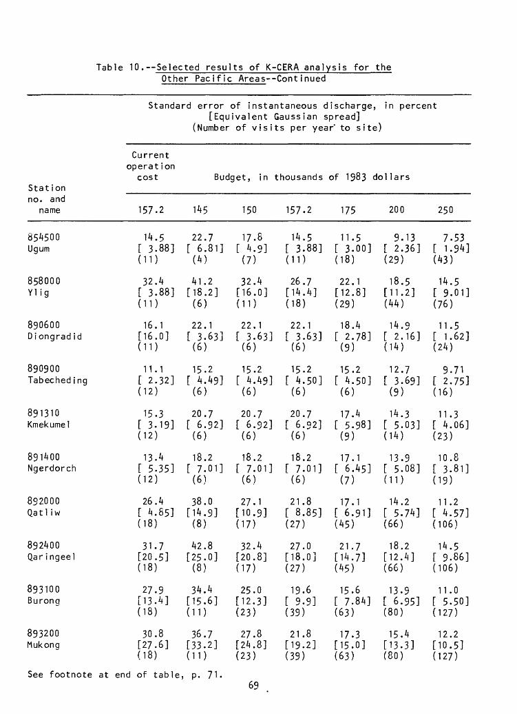
Table 10.--Selected results of K-CERA analysis for theOther Pacific Areas Cent inued
Standard error of instantaneous discharge, in percent [Equivalent Gaussian spread]
(Number of visits per year' to site)
Station no. and
name
854500 Ugum
858000 Ylig
890600 Diongradid
890900 Tabecheding
891310 Kmekumel
891400 Ngerdorch
892000 Qatl iw
892400 Qar ingeel
893100 Burong
893200 Mukong
Currentoperat ion
cost
157.2
14.5 [ 3.88] (11)
32.4 [ 3.88] (11)
16.1 [16.0] (11)
11.1 [ 2.32] (12)
15.3 [ 3.19] (12)
13.4 [ 5.35] (12)
26.4 [ 4.85] (18)
31.7 [20.5] (18)
27.9 [13.4] (18)
30.8 [27.6] (18)
Budget, in thousands
145
22.7 [ 6.81] (4)
41.2 [18.2] (6)
22.1 [ 3.63] (6)
15.2 [ 4.49] (6)
20.7 [ 6.92] (6)
18.2 [ 7.01] (6)
38.0 [14.9] (8)
42.8 [25.0] (8)
34.4 [15.6] (11)
36.7 [33.2](11)
150
17.8 [ 4.9] (7)
32.4 [16.0] (11)
22.1 [ 3.63] (6)
15.2 [ 4.49] (6)
20.7 [ 6.92] (6)
18.2 [ 7.01] (6)
27.1 [10.9] (17)
32.4 [20.8] (17)
25.0 [12.3] (23)
27.8 [24.8] (23)
157.2
14.5 [ 3.88](11)
26.7 [14.4] (18)
22.1 [ 3.63] (6)
15.2 [ 4.50] (6)
20.7 [ 6.92] (6)
18.2 [ 7.01] (6)
21.8 [ 8.85] (27)
27.0 [18.0] (27)
19.6 [ 9.9] (39)
21.8 [19.2] (39)
of 1983 dollars
175
11.5 [ 3.00] (18)
22.1 [12.8] (29)
18.4 [ 2.78] (9)
15.2 [ 4.50] (6)
17.4 [ 5.98] (9)
17.1 [ 6.45] (7)
17.1 [ 6.91] (45)
21.7 [14.7] (45)
15.6 [ 7.84] (63)
17.3 [15.0] (63)
200
9.13 [ 2.36] (29)
18.5 [11.2] (44)
14.9 [ 2.16] (14)
12.7 [ 3.69] (9)
14.3 [ 5.03] (14)
13.9 [ 5.08](11)
14.2 [ 5.74] (66)
18.2 [12.4] (66)
13.9 [ 6.95] (80)
15.4 [13.3] (80)
250
7.53 [ 1.94] (43)
14.5 [ 9.01] (76)
11.5 [ 1.62] (24)
9.71 [ 2.75] (16)
11.3 [ 4.06] (23)
10.8 [ 3.81] (19)
11.2 [ 4.57] (106)
14.5 [ 9.86] (106)
11.0 [ 5.50] (127)
12.2 [10.5] (127)
See footnote at end of table, p. 71.69
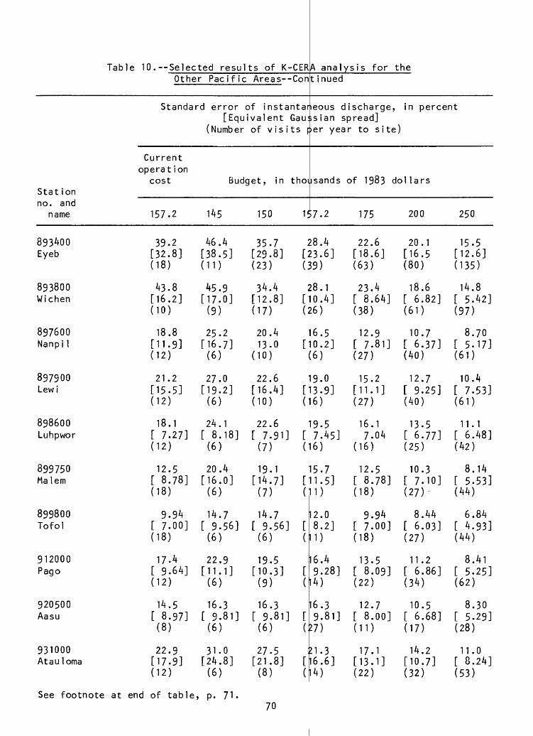
Stat ionno. and
name
893400Eyeb
893800Wichen
897600Nanpi 1
897900Lewi
898600Luhpwor
899750Malem
899800Tofol
912000Pago
920500Aasu
931000Atauloma
Table 10. --Selected results of K-CEROther Pacific Areas--Con
Standard error of instantar
Currentoperat ion
cost
157.2
39.2[32.8](18)
43.8[16.2](10)
18.8[11.9](12)
21.2[15.5](12)
18.1[ 7.27](12)
12.5[ 8.78](18)
9.94[ 7.00](18)
17.4[ 9.64](12)
14.5[ 8.97](8)
22.9[17.9](12)
[Equivalent Gau;(Number of vis its \
Budget, in thoi
145 150 1{
46.4 35.7 :[38.5] [29.8] [!(11) (23) C
45.9 34.4 :[17.0] [12.8] [(9) (17) C
25.2 20.4[16.7] 13.0 [(6) (10)
27.0 22.6[19.2] [16.4] [(6) (10) (
24.1 22.6[ 8.18] [ 7.91] [(6) (7) (
20.4 19.1[16.0] [14.7] [(6) (7) (
14.7 14.7[ 9.56] [ 9.56] [(6) (6) (
22.9 19.5[11.1] [10.3] [(6) (9) (
16.3 16.3[ 9.81] [ 9.81] [(6) (6) (:
31.0 27.5 :[24.8] [21.8] [(6) (8) (
A analysis fort inued
leous discharge>sian spread]
the
, in percent
>er year to site)
jsands of 1983
57.2 175
>8.4 22.6>3.6] [18.6]59) (63)
>8.1 23.40.4] [ 8.64]>6) (38)
6.5 12.90.2] [ 7.81]6) (27)
9.0 15.23.9] [11.1]6) (27)
9.5 16.17.45] 7.046) (16)
5.7 12.51.5] [ 8.78]1) (18)
2.0 9.948.2] [ 7.00]D (18)
6.4 13.59.28] [ 8.09]4) (22)
6.3 12.79.81] [ 8.00]11} (11)
M.3 17.116.6] [13.1]4) (22)
dol lars
200
20.1[16.5(80)
18.6[ 6.82](61)
10.7[ 6.37](40)
12.7[ 9.25](40)
13.5[ 6.77](25)
10.3[ 7.10](27)
8.44[ 6.03](27)
11.2[ 6.86](34)
10.5[ 6.68](17)
14.2[10.7](32)
250
15.5[12.6](135)
14.8[ 5.42](97)
8.70[ 5.17](61)
10.4[ 7.53](61)
11.1[ 6.48](42)
8.14[ 5.53](44)
6.84[ 4.93](44)
8.41[ 5.25](62)
8.30[ 5.29](28)
11.0[ 8.24](53)
See footnote at end of table, p. 71.70
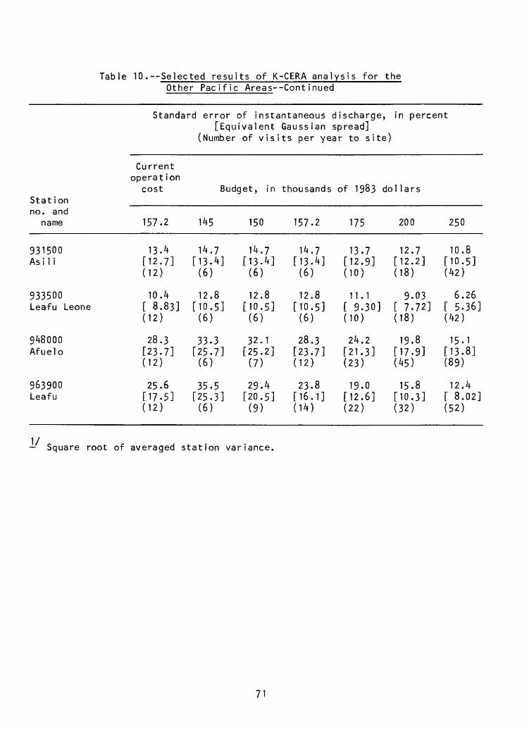
Table 10. Selected results of K-CERA analysis for theOther Pacific Areas--Cont inued
Standard error of instantaneous discharge, in percent [Equivalent Gaussian spread]
(Number of visits per year to site)
Stat ion no. and
name
931500 Asi 1 i
933500 Leafu Leone
948000 Afuelo
963900 Leafu
Current operat ion
cost
157.2
13.4 [12.7] (12)
10.4 [ 8.83] (12)
28.3 [23.7] (12)
25.6 [17.5] (12)
Budget, in thousands
145
14.7 [13.4] (6)
12.8 [10.5] (6)
33.3 [25.7] (6)
35.5 [25.3] (6)
150
14.7 [13.4] (6)
12.8 [10.5] (6)
32.1 [25.2] (7)
29.4 [20.5] (9)
157.2
14.7 [13.4] (6)
12.8 [10.51 (6)
28.3 [23.7] (12)
23.8 [16.1] (14)
of 1983 dollars
175
13.7 [12.9] (10)
11.1 [ 9.30] (10)
24.2 [21.3] (23)
19.0 [12.6] (22)
200
12.7 [12.2](18)
9.03 [ 7.72] (18)
19.8 [17.9] (45)
15.8 [10.3] (32)
250
10.8 [10.5] (42)
6.26 [ 5.36] (42)
15.1 [13.8] (89)
12.4 [ 8.02] (52)
Square root of averaged station variance.
71

to
mi
The
(Kahoma)
averacie
A minimum budget of $370,000 is required
for the State of Hawaii; a budget less than thi
and maintenance of the gages and recorders. Sta
from the program if the budget fell below this
the average standard error is 23.7 percent,
percent would occur at station 541000 (Koolau
56.0 percent would occur at station 638500
As explained earlier, stations 303000 (Pun
included in the calculations for standard error:
The maximum budget analyzed for the State
which resulted in an average standard error of e
$550,000 budget, the extremes of standard error a
(Koolau Haipuena), and 44.1 percent at station
apparent that improvements in accuracy of streanf
larger budgets become available.
It would be possible to reduce the
Pacific Areas by a policy change while maintain
In this case, the average standard error would
percent. Extremes of standard error in indivi
percent for stations 899800 (Tofol) and 801000
A minimum budget of $145,000 is required
for the Other Pacific Areas; a budget less
service and maintenance of the gages and record
eliminated from the program if the budget fel
minimum budget, the average standard error is 32.
error of 12.8 percent would occur at station !
maximum of 52.1 percent would occur at station
The maximum budget analyzed for the
$250,000, which resulted in an average stand
percent. For the $250,000 budget, the extremes
at station 933500 (Leafu Leone), and 25-3 percent
Thus, it is apparent that significant i
records can be obtained if larger budgets becom
operate the 92-station program
does not permit proper service
ions would have to be eliminated
nimum. At the minimum budget,
minimum standard error of 3.4
Haipuena), while the maximum of
«Huu) and 899620 (Melo) were not
of Hawaii program was $550,000,
stimate of 12.9 percent. For the
re 2.1 percent at station 541000
414000 (Kaunakakai). Thus, it is
low records can be obtained if
to
than
improvements
standard error for the Other
ng the same budget of $157,250.
decrease from 25.9 percent to 23.2
dual sites would be 12 and 52
Talofofo), respectively,
operate the 32-station program
this does not permit proper
lers. Stations would have to be
1 below this minimum. At the
0 percent. The minimum standard
933500 (Leafu Leone), while the
1000 (Talofofo).
Ot ler Pacific Areas program was
rd error of estimate of 12.2
f standard error are 6.3 percent
at station 801000 (Talofofo).
in accuracy of streamflow
ava ilable.
72
Conclusions from the K-CERA Analysis
As a result of the K-CERA analysis, the following suggestions are offered:
1. The policy for the definition of field activities in the stream-gaging
program should be altered to improve the current average standard
errors of estimate of streamflow records to 17-7 percent with the
current budget of $413,400 for the State of Hawaii and 23.2 percent
with the current budget of $157,200 for the Other Pacific Areas. This
shift would result in some increases and some decreases in accuracy of
records at individual sites.
2. After implementing the first suggestion, the amount of funding for
stations with accuracies that are not acceptable for the data uses
should be renegotiated with the data users.
3. The funding made available by implementation of the second suggestion
should be used to improve the accuracy of records at appropriate
stations to an acceptable level.
4. Schemes for reducing the probabilities of missing record, for example
increased use of local gage observers and satellite relay of data,
should be explored and evaluated as to their cost-effectiveness in
providing streamflow information.
73
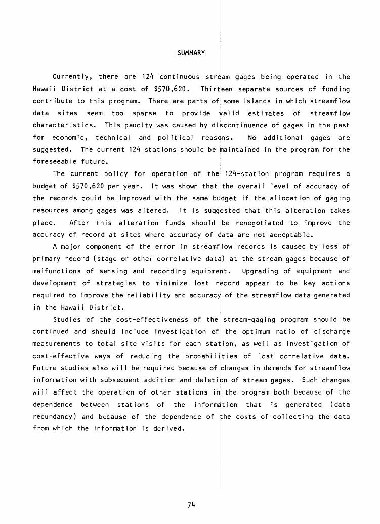
SUMMARY
stream
va
reasons
Currently, there are \2k continuous
Hawaii District at a cost of $570,620. Thi
contribute to this program. There are parts of
data sites seem too sparse to provide
characteristics. This paucity was caused by di
for economic, technical and political
suggested. The current 124 stations should be
foreseeable future.
The current policy for operation of the
budget of $570,620 per year. It was shown that
the records could be improved with the same
resources among gages was altered. It is
place. After this alteration funds should
accuracy of record at sites where accuracy of
A major component of the error in streamfl
primary record (stage or other correlative date
malfunctions of sensing and recording equipment
development of strategies to minimize lost
required to improve the reliability and accuracy
in the Hawaii District.
Studies of the cost-effectiveness of the
continued and should include investigation of
measurements to total site visits for each stat
cost-effective ways of reducing the probabili
Future studies also will be required because of
information with subsequent addition and deleti
will affect the operation of other stations in
dependence between stations of the informat
redundancy) and because of the dependence of
from which the information is derived.
gages being operated in the
rteen separate sources of funding
some islands in which streamflow
lid estimates of streamflow
iscont inuance of gages in the past
No additional gages are
maintained in the program for the
124-station program requires a
the overall level of accuracy of
budget if the allocation of gaging
suggested that this alteration takes
be renegotiated to improve the
data are not acceptable,
ow records is caused by loss of
) at the stream gages because of
Upgrading of equipment and
record appear to be key actions
of the streamflow data generated
stream-gaging program should be
the optimum ratio of discharge
ion, as well as investigation of
ties of lost correlative data.
changes in demands for streamflow
on of stream gages. Such changes
the program both because of the
ion that is generated (data
the costs of collecting the data
REFERENCES CITED
Benson, M. A., and Carter, R. W., 1973, A national study of the streamflow data-
collection program: U.S. Geological Survey Water-Supply Paper 2028, 44 p.
Carter, R. W., and Benson, M. A., 1970, Concepts for design of streamflow data
programs: U.S. Geological Survey Open-File Report, 33 p.
Draper, N. R., and Smith, H., 1966, Applied regression analysis: New York,
N. Y., John Wiley and Sons, 2d ed., 709 p.
Fontaine, R. A., Moss, M. E., Smath, J. A., and Thomas, W. 0., Jr., 1984, Cost-
effectiveness of the stream-gaging program in Maine a prototype for
nation-wide implementation: U.S. Geological Survey Water-Supply Paper
2244, 39 p.
Gelb, A., ed., 1974, Applied optimal estimation: The Massachusetts Institute of
Technology Press, Cambridge, Mass., 374 p.
Gilroy, E. J., and Moss, M. E., 1981, Cost-effective stream-gaging strategies for
the Lower Colorado River Basin: U.S. Geological Survey Open-File Report Si-
1019, 42 p.
Hutchinson, N. E., 1975, WATSTORE User's guide, volume 1: U.S. Geological Survey
Open-File Report 75-426, 791 p.
Keefer, T. N., 1974, Desktop computer flow routing: American Society of Civil
Engineers Proceedings, Journal of the Hydraulics Division, v. 100, no. HY7,
p. 1047-1058.
Keefer, T. N., and McQuivey, R. S., 1974, Multiple linearization flow routing
model: American Society of Civil Engineers Proceedings, Journal of the
Hydraulics Division, v. 100, no. HY7, p. 1031-1046.
Kleinbaum, D. G., and Kupper, L. L., 1978, Applied regression analysis and other
multivariable methods: North Scituate, Mass., Duxbury Press, 556 p.
Mitchell, W. D., 1962, Effect of reservoir storage on peak flow: U.S. Geological
Survey Water-Supply Paper 1580, p. C1-C25.
Moss, M. E., and Gilroy, E. J., 1980, Cost-effective stream-gaging strategies for
the Lower Colorado River Basin: U.S. Geological Survey Open-File Report 80-
1048, 111 p.
Moss, M. E., Gilroy, E. J., Tasker, G. D., and Karlinger, M. R., 1982, Design of
surface-water data networks for regional information: U.S. Geological
Survey Water-Supply Paper 2178, 33 p.
75
cs
Riggs, H. C., 1973, Regional analysis of
Geological Survey Techniques of Water-
chapter B3, 15 p.
Thomas, D. M., and Benson, M. A., 1970, Genera
istics from drainage-basin characteristi
Supply Paper 1975, 55 p.
U.S. Geological Survey, 1981, Water resources
U.S. Geological Survey Water-Data Report
- 1981, Water resources data for Hawaii and
1981: U.S. Geological Survey Water-Datu
Territory of the Pacific Islands, Guam
Mariana Islands, 148 p.
streamflow characteristics: U.S.
Resources Investigations, book 4,
ization of streamflow character-
U.S. Geological Survey Water-
data, Hawaii, water year 1981:
-81-1, v. 1. Hawai i, 266 p.
other Pacific areas, water year
Report HI-81-2, v. 2. Trust
, American Samoa, and Northern
76