Evaluation of Technical Efficiency in Indian Sugar ... · PDF filesugar factories and firms with access to sweater cane are more efficient. Further, public-owned firms are found to

Eurasian Journal of Business and Economics 2012, 5 (9), 57-78.

Evaluation of Technical Efficiency in Indian

Sugar Industry: An Application of Full

Cumulative Data Envelopment Analysis

Sunil KUMAR,* Nitin ARORA

**

Abstract

This study focuses on the inter-temporal and inter-state variations in technical and

scale efficiency levels of Indian sugar industry. In the first stage, full cumulative data

envelopment analysis (FCDEA) is used to derive efficiency scores for 12 major sugar

producing states. The panel data truncated regression is employed in the second

stage to assess the key factors explaining the observed variations in the efficiency

levels. The results suggest that the extent of technical inefficiency in Indian sugar

industry is about 35.5 percent per annum, and the observed technical inefficiency

stems primarily due to managerial inefficiency rather scale inefficiency. Also, a

precipitous decline in the level of technical efficiency has been noticed in the post-

reforms period relative to the level observed in the pre-reforms period. The

availability of skilled labour and profitability have been found to be most significant

determinants of technical efficiency in Indian sugar industry.

Keywords: Data Envelopment Analysis, Bootstrapping, Indian Sugar Industry

JEL Code Classification: C02, C69, D24

*

Associate Professor, Faculty of Economics, South Asian University, New Delhi, India. Email: [email protected] **

Assistant Professor, Department of Economics, Panjab University, Chandigarh, India. Email:

[email protected]

Sunil KUMAR & Nitin ARORA

Page | 58 EJBE 2012, 5 (9)

1. Introduction

The present study has been undertaken with the primary objective to evaluate the

technical efficiency in Indian sugar industry. The relevance of the study stems from

the facts that sugar industry: i) is the second largest agro-based industry in India

after the cotton-textile; ii) provides direct employment to 0.5 million and indirect

employment to 55 million skilled and unskilled workers (Sanyal et al., 2008); iii)

contributes Rs. 25 billion annually to the centre and state exchequer in the form of

taxes; iv) has a potential to generate 5000MW surplus power through the process

of cogeneration; and v) supports the petroleum blending program through the

production of ethanol using molasses1 (Indian Sugar Mills Association, 2008).

Despite all of these facts, the sugar industry in India has been offended by the

ignorance of policy planners and there are over 162 sugar mills in the country,

which are considered as sick (Minister of State for Food and Agriculture Mr. K. V.

Thomas said in a response to a written query in the Lok Sabha, 2010)2. The figure of

sickness is high by all standards and thus, demonstrates the abysmal status of the

health of Indian sugar industry. Thus, there is an urgent need to analyze the

efficiency performance of the Indian sugar industry at both aggregated and

disaggregated regional levels3.

It has been well acknowledged by the industry experts that the dismal performance

of sugar industry is the product of both internal and external environmental

factors. The external factors are primarily uncontrollable from the management

point of view (like decreasing area under sugarcane cultivation, tight government

regulations in pricing and distribution of sugar, rainfall deficit, etc.) and their effect

is almost uniform on the overall performance of the industry. However, the internal

factors which are largely controllable in nature (like low level of capacity utilization,

inefficient use of inputs, labour unrest, and managerial underperformance, etc.)

also contribute to a dismal performance of the sugar industry, but their effect

varies from one sugar mill to another. Through the present study, an attempt has

been made to analyze the effect of both internal and external factors on the

growth performance of Indian sugar industry. The overall technical efficiency (OTE)

score has been used as the yardstick of performance, which depends upon the

internal sources of managerial (proxied by pure technical efficiency (PTE)) and scale

efficiencies (SE) as well as external sources like profitability, availability of skilled

manpower and capital intensity, etc.

The concept of technical efficiency is intrinsically related to the estimation of a

production frontier since efficiency measures can only be defined with respect to a

benchmark i.e., an ideal level of performance. A technically efficient firm would be

one that produces the maximum possible output(s) from a given set of inputs or

1 A byproduct of the sugar manufacturing process.

2 See <<http://www.business-standard.com/india/news/162-sugar-mills-in-indiasick-thomas/116929/on>>

published on November 23, 2010. Information accessed on August 2, 2011. 3 see, Pandey (2007), and Kumar and Arora (2009) for an introductory review of Indian sugar industry.

Evaluation of Technical Efficiency in Indian Sugar Industry: An Application of …

EJBE 2012, 5 (9) Page | 59

one that produces a certain level of output(s) with the minimum amount of inputs.

The literature on the measurement of technical efficiency provides two competing

approaches for estimating the relative efficiency across firms using the best-

practice frontier: i) non-parametric data envelopment analysis (DEA) approach; and

ii) parametric stochastic frontier analysis (SFA) approach (see, Charnes et al. (1994)

and Kumbhakar and Lovell (2003) for details on DEA and SFA methods,

respectively). In parametric approach, a specific functional form of the production

function like Cobb-Douglas and Translog, etc. is required to specify a-priori

technical relationship between inputs and output. This efficiency is then assessed in

relation to this function with constant parameters and will be different depending

on the chosen functional form. In contrast, nonparametric approaches do not

specify a functional form and involve solving linear program, in which an objective

function envelops the observed data; then efficiency scores are derived by

measuring how far an observation is from the envelop or frontier. A technically

efficient firm operates at the best-practice frontier and will attain an efficiency

score equal to 1, whereas the firm operating beneath the best-practice levels is

deemed to be technically inefficient, and its efficiency score lies between 0 and 1.

However, no consensus has been reached in the literature about the appropriation

and preferred estimation methods. For getting a convenient decomposition of

technical efficiency, this paper uses DEA to estimate empirically technical, pure and

scale efficiency scores.

To achieve the underlined objectives of the study, the balance of the paper is set

out as follows: Section 2 provides a review of literature on the efficiency evaluation

of Indian sugar industry. Section 3 presents the methodology used in the present

study to compute the technical and scale efficiency measures. However, Section 4

is empirical in nature, and major findings of this study are presented here. The

impact of different environmental variables on the different efficiency measures

has also been discussed in this section. The final section concludes the study and

provides a few relevant policy implications.

2. Review of Literature

Ferrantino and Ferrier (1995) utilized panel data of 239 sugar mills for the period

1980/81 to 1984/85, and analyzed the technical efficiency of Vacuum-Pan Sugar

industry of India using the technique of SFA. The study concluded that the smaller

sugar factories and firms with access to sweater cane are more efficient. Further,

public-owned firms are found to be less efficient than the private and co-operative

sugar firms.

Ferrantino et al. (1995) examined the effect of organizational form on the efficiency

of Indian sugar industry. Using the panel data set for 126 sugar firms, covering the

period from 1980/81 to 1984/85, the study observed average TE score of 0.85. The

study concluded that the majority of sugar factories were operating close to the

efficient frontier. The evidence pertaining to the organizational differences among


Page | 60 EJBE 2012, 5 (9)

the sugar firms confirms that there exists a slight difference between the efficiency

of co-operative, public, and private sugar factories.

Ferrantino and Ferrier (1996), using the dataset of 122 sugar firms covering the

period from 1981/82 to 1985/86, made an attempt to measure the levels of

technical efficiency and productivity growth in the Indian sugar industry. An

average efficiency score of 0.97 has been observed over the study period of five

years. The factories with the greatest licensed capacity (i.e., greater than 3000

tonns crushed per day) were on average the most technically and scale efficient

among the five size classes analyzed. Further, statistically significant productivity

gains have been realized in 1982/83 and 1985/86, while productivity declined in

1984/85 and remained constant in 1983/84.

Murty et al. (2006), using the survey of polluting industries in India (conducted for

1996/97, 1997/98 and 1998/99), tried to analyze the impact of environmental

regulation on productive efficiency and cost of pollution abatement for the sugar

industry of India. The average environmental efficiency has been observed to be

0.85, implying the industry has to incur an input cost of 15 percent more to reduce

pollution for a given level of production of good output. The results of Malmquist

productivity index, used to measures changes in the TFP of firms, found to be

sensitive to the environmental constraints i.e., the increase in TFP is almost 200

percent without binding environmental constraints while it increases only by 10

percent with these constraints.

Singh (2006a) utilized data for 65 private sugar mills operating in six major states

viz., Uttar Pradesh (U.P.), Bihar, Punjab, Andhra Pradesh, Karnataka, and Tamil

Nadu obtained from Prowess database provided by Center for Monitoring Indian

Economy (CMIE), to analyze technical and scale efficiencies in the Indian sugar

mills. Using the nonparametric DEA technique the study observed that 38 percent

and 60 percent of sugar mills have attained the status of globally and locally

(efficient under VRS assumption) efficient firms respectively. The prevalence of

increasing returns-to-scale (IRS) has been observed in 60 percent of the inefficient

sugar mills, signifying the urgent need of increasing the plant size.

Singh (2006b) utilized the technique of DEA to analyze the efficiency of 36 sugar

mills of Uttar Pradesh (U.P.) operating during the year 2003/04. The study observed

the prevalence of 9 percent inefficiency among the selected sugar firms. It has been

also observed that 14 percent of sugar mills attained efficiency score equal to 1

and, thus, identified as globally efficient under the constant returns-to-scale

technology. A pressing need for capacity expansion of sugar mills has also been

notified because most of the sugar mills are found to be operating in the zone of

increasing returns-to-scale. The post-DEA regression analysis reveal that net sugar

recovery and plant size encompass a significant and positive effect on overall

technical efficiency and scale efficiency of the sugar mills of UP.


EJBE 2012, 5 (9) Page | 61

Singh (2007) attempted to analyze the performance of sugar mills in U.P. by

ownership, size and location using the dataset for 36 sugar firms over the period

1996/97 to 2002/03. Applying the method of DEA, the study concluded that the

sample firms operate at a high level of efficiency and the magnitude of inefficiency

is only 7 percent. Owing to the differences in ownership, size and location of the

mills, the performance of sugar mills diverge significantly. Further, the mills in the

western region of UP are found to be more efficient than the central and eastern

regions. However, the problem of surplus labour is found to be serious, as 43

percent reduction is theoretically possible in the labour input so as the sugar firms

in UP can become labour efficient.

Singh et al. (2007), seeks to examine economic efficiency of sugar industry in Uttar

Pradesh. Using the data for 63 sugar mills of U.P. for the year 2001/02, the study

estimated stochastic production frontier and detected an average efficiency to the

tune of 73.5 percent in the sugar industry of UP. However, the firm specific

inefficiency levels found to be ranging from 8 percent to 55 percent. Further, the

private sector sugar factories in the western region of UP attained the maximum

average efficiency score of 84.29 percent, and thus, found to be belonging to “most

efficient category”. The evidences regarding the ownership structure reveal that

the cooperative sector mills in the eastern region of UP are classified under the

category of “least efficient group”.

To the best of our knowledge, there exists no published study which concentrates

on analyzing inter-temporal and inter-state variations in the technical efficiency of

Indian sugar industry. The present study is an endeavor in this direction and tries to

fill up the existing void in the literature. The present study has two principal

objectives: i) the first objective is to analyze the inter-temporal and inter-state

variations in technical efficiency of Indian sugar industry; and ii) the second is to

identify the factors influencing the technical efficiency in Indian sugar industry

using panel data Tobit regression analysis.

3. Methodological Framework

As noted above, we applied DEA for obtaining technical, pure technical and scale

efficiency scores for sugar industry at national and state levels. In their seminal

paper, Charnes, Cooper and Rhodes (1978) developed a ‘data oriented’ method

based on linear programming technique and coined it as Data Envelopment

Analysis (DEA) for estimating the relative technical efficiency of a set of peer

entities called Decision Making Units (DMUs)4. DEA floats a piecewise linear surface

to the rest on top of the observations (Seiford and Thrall, 1990). The DMUs that lie

on the frontier are the best-practice institutions and retain a technical efficiency

score of one. Those DMUs enveloped by the extremal surface are scaled against a

4 Throughout this paper and consistent with DEA terminology, the term ‘decision making unit’ or ‘DMU’

will refer to the individuals in the evaluation group. In the context of present application, it will refer

specifically to the sugar producing states of India.


Page | 62 EJBE 2012, 5 (9)

convex combination of the DMUs on the frontier facet closest to it and have values

somewhere between 0 and 1.

The above conceptualization of the concept of technical efficiency is based upon

the assumption of constant returns-to-scale (CRS). In DEA literature, the measure

of technical efficiency corresponding to CRS assumption is generally referred as

overall technical efficiency (OTE)5 which captures the efficiency due to both

managerial and scale effects. The CRS assumption is only appropriate if all DMUs

are operating at an optimal scale. When DMUs are not operating at optimal scale

(i.e., variable returns-to-scale (VRS) prevails), the overall technical efficiency (OTE)

can be decomposed into pure technical efficiency (PTE)6 and scale efficiency (SE).

The PTE measure provides a sort of managerial efficiency i.e., the capability of the

management to convert the inputs into outputs. However, the SE measure

indicates whether the DMU in question is operating at optimal scale size or not.

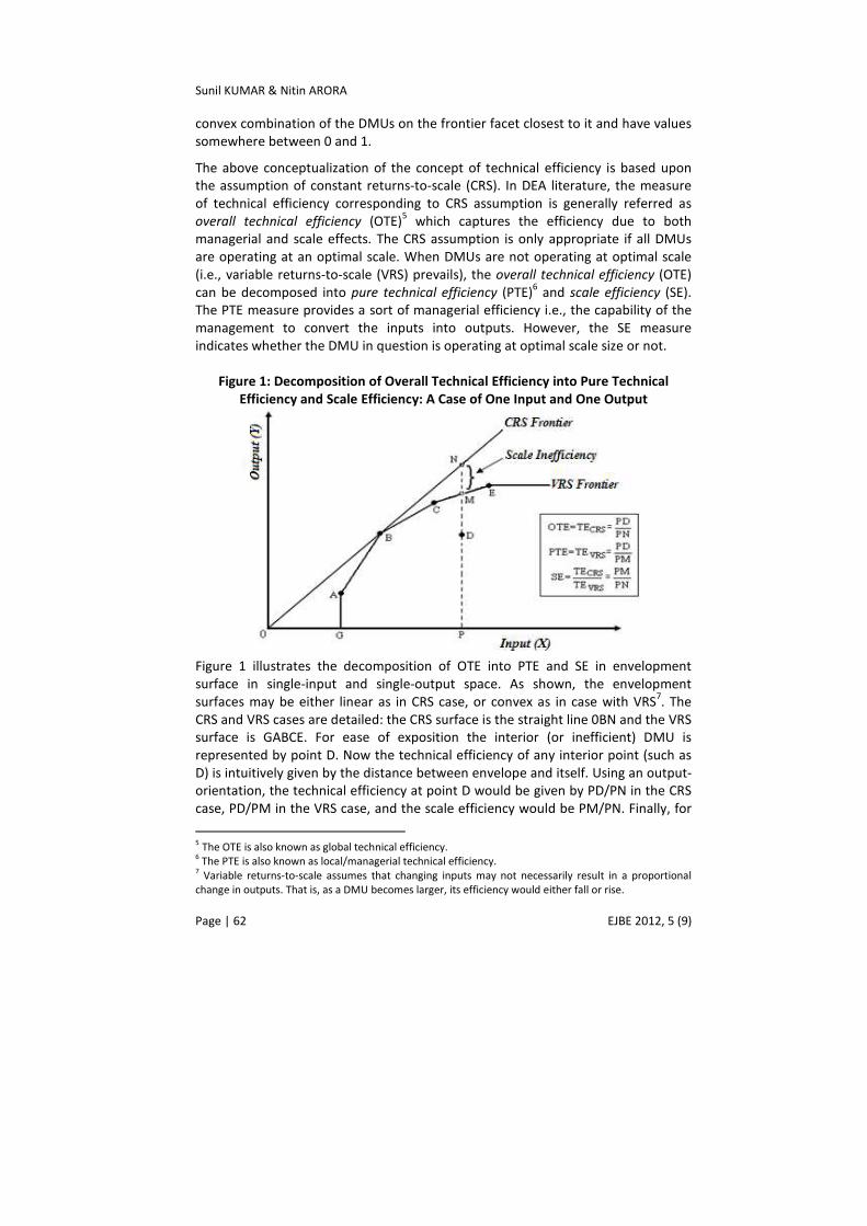
Figure 1: Decomposition of Overall Technical Efficiency into Pure Technical

Efficiency and Scale Efficiency: A Case of One Input and One Output

Figure 1 illustrates the decomposition of OTE into PTE and SE in envelopment

surface in single-input and single-output space. As shown, the envelopment

surfaces may be either linear as in CRS case, or convex as in case with VRS7. The

CRS and VRS cases are detailed: the CRS surface is the straight line 0BN and the VRS

surface is GABCE. For ease of exposition the interior (or inefficient) DMU is

represented by point D. Now the technical efficiency of any interior point (such as

D) is intuitively given by the distance between envelope and itself. Using an output-

orientation, the technical efficiency at point D would be given by PD/PN in the CRS

case, PD/PM in the VRS case, and the scale efficiency would be PM/PN. Finally, for

5 The OTE is also known as global technical efficiency. 6 The PTE is also known as local/managerial technical efficiency.

7 Variable returns-to-scale assumes that changing inputs may not necessarily result in a proportional

change in outputs. That is, as a DMU becomes larger, its efficiency would either fall or rise.


EJBE 2012, 5 (9) Page | 63

the DMU on the envelopment surface, such as denoted by B, the technical

efficiency measure for both VRS and CRS would be identical as DMU B is found to

be operating at CRS as well as VRS frontier.

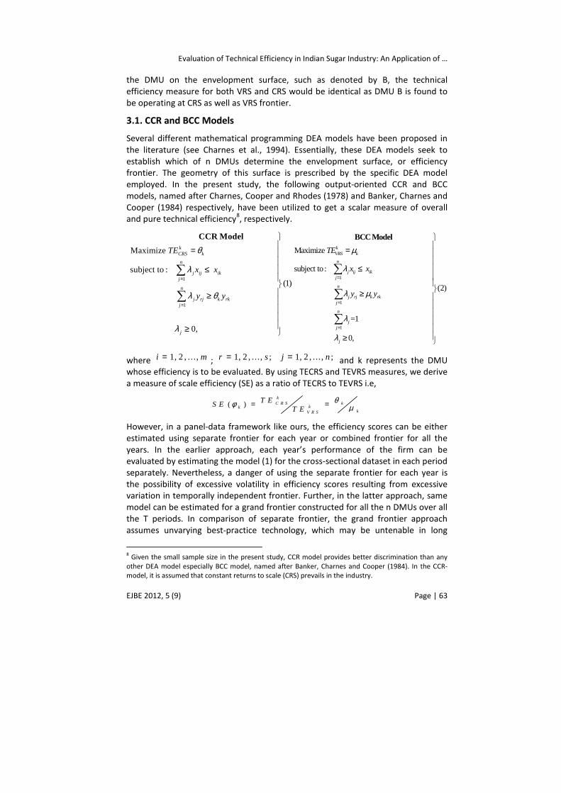
3.1. CCR and BCC Models

Several different mathematical programming DEA models have been proposed in

the literature (see Charnes et al., 1994). Essentially, these DEA models seek to

establish which of n DMUs determine the envelopment surface, or efficiency

frontier. The geometry of this surface is prescribed by the specific DEA model

employed. In the present study, the following output-oriented CCR and BCC

models, named after Charnes, Cooper and Rhodes (1978) and Banker, Charnes and

Cooper (1984) respectively, have been utilized to get a scalar measure of overall

and pure technical efficiency8, respectively.

1

1

Maximize

subject to :

0,

kCRS k

n

j ij ikj

n

j rj k rkj

j

TE

x x

y y

θ

λ

λ θ

λ

=

=

=

≤

≥

≥

∑

∑

CCR Model

(1)

1

1

Maximize

subject to :

kVRS k

n

j ij ikj

n

j rj k rkj

TE

x x

y y

µ

λ

λ µ

=

=

=

≤

≥

∑

∑

BCC Model

1

(2)

=1

0,

n

jj

j

λ

λ=

≥

∑

where 1, 2 , ...,i m= ; 1, 2 , ..., ;r s= 1, 2 , ..., ;j n= and k represents the DMU

whose efficiency is to be evaluated. By using TECRS and TEVRS measures, we derive

a measure of scale efficiency (SE) as a ratio of TECRS to TEVRS i.e,

( )k

C R S kkk

kV R S

T ES ET E

θφ µ= =

However, in a panel-data framework like ours, the efficiency scores can be either

estimated using separate frontier for each year or combined frontier for all the

years. In the earlier approach, each year’s performance of the firm can be

evaluated by estimating the model (1) for the cross-sectional dataset in each period

separately. Nevertheless, a danger of using the separate frontier for each year is

the possibility of excessive volatility in efficiency scores resulting from excessive

variation in temporally independent frontier. Further, in the latter approach, same

model can be estimated for a grand frontier constructed for all the n DMUs over all

the T periods. In comparison of separate frontier, the grand frontier approach

assumes unvarying best-practice technology, which may be untenable in long

8 Given the small sample size in the present study, CCR model provides better discrimination than any

other DEA model especially BCC model, named after Banker, Charnes and Cooper (1984). In the CCR-

model, it is assumed that constant returns to scale (CRS) prevails in the industry.


Page | 64 EJBE 2012, 5 (9)

panels (Fried et al., 2008). Further, in our case, 12 data points (i.e., sugar producing

states) provide too few degrees of freedom when the production process is four-

dimensional i.e., comprises three inputs (i.e., capacity adjusted GFC, intermediate

inputs and labour) and one output (i.e., gross output). Bankers et al. (1984)

proposed a rule that the number of observations used to project the efficient

frontier should not be smaller than 3(m+s), where m is the number of inputs and s

is the number of outputs. For our four-dimension problem, this suggests a number

of DMUs must be greater than 12 for each cross-section. Same problem was faced

by Nighiem and Coelli (2002), while applying DEA to analyze the productivity

change in Vietnamese rice production. Helvoigt and Adams (2008) had also

experienced the same hurdle while obtaining technical efficiency and productivity

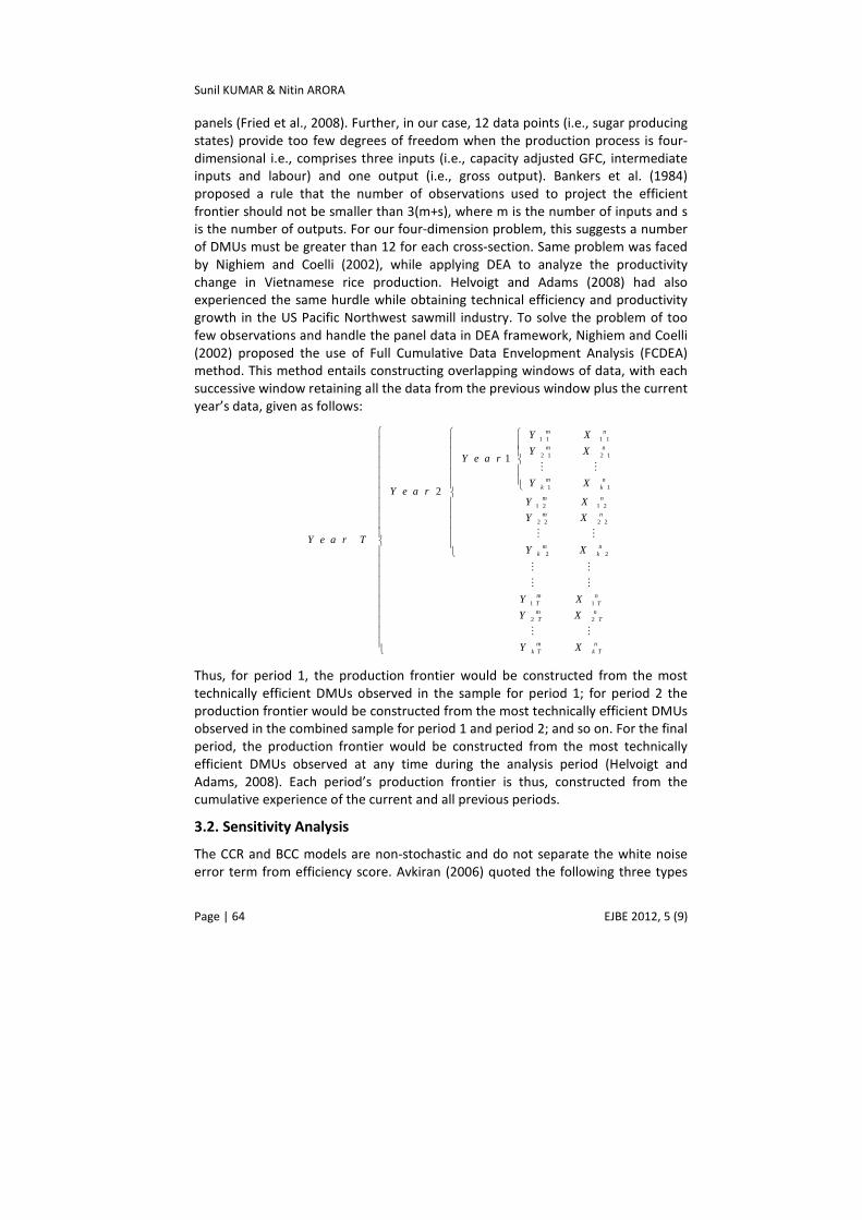
growth in the US Pacific Northwest sawmill industry. To solve the problem of too

few observations and handle the panel data in DEA framework, Nighiem and Coelli

(2002) proposed the use of Full Cumulative Data Envelopment Analysis (FCDEA)

method. This method entails constructing overlapping windows of data, with each

successive window retaining all the data from the previous window plus the current

year’s data, given as follows:

1 1 1 1

2 1 2 1

1 1

1 2 1 2

2 2 2 2

2 2

1 1

2 2

1

2

m n

m n

m nk k

m n

m n

m nk k

m nT T

m nT T

m nk T k T

Y X

Y XY e a r

Y XY e a r

Y X

Y X

Y e a r TY X

Y X

Y X

Y X

M M

M M

M M

M M

M M

Thus, for period 1, the production frontier would be constructed from the most

technically efficient DMUs observed in the sample for period 1; for period 2 the

production frontier would be constructed from the most technically efficient DMUs

observed in the combined sample for period 1 and period 2; and so on. For the final

period, the production frontier would be constructed from the most technically

efficient DMUs observed at any time during the analysis period (Helvoigt and

Adams, 2008). Each period’s production frontier is thus, constructed from the

cumulative experience of the current and all previous periods.

3.2. Sensitivity Analysis

The CCR and BCC models are non-stochastic and do not separate the white noise

error term from efficiency score. Avkiran (2006) quoted the following three types


EJBE 2012, 5 (9) Page | 65

of errors discussed by Fethi and Jones (2006): i) measurement error occurs when

the data used contain random errors of reporting and recording; ii) sampling error

which arises when the data refer only to a subset of the possible populations of

values that could have been recorded; and iii) specification errors come up when

we are unsure of the underlying theoretical or population model which describes

agents’ behavior. Thus, the interpretations regarding the efficiency levels may be

misleading in the presence of a significant white-noise error term. To overcome this

drawback, several attempts have been made to seprate the white-noise error term

from DEA based efficiency scores and thus, ensure the robustness of these

estimates. The techniques of Stochastic DEA, Stochastic Non-Parametric

Envelopment of Data (StoNED), and Bootstrapping DEA have been suggested for

separating the white-noise error term in a DEA framework. Amongst all these

techniques, the Bootstrapping DEA is the most popular approach to separate

random noise (see, Fried et al., 2008). The first use of bootstrap in frontier models

dates to Simar (1992). However, its use for nonparametric envelopment estimators

was developed by Ferrier and Hirschberg (1997), Simar and Wilson (1998, 2000a)

and the theoretical properties of the bootstrap with DEA estimators are provided in

Kneip et al. (2003). While using the bootstrapping techniuqes, Efron and Tibshirani

(1993) and Simar and Wilson (1999) note that the bias-corrected estimators of

distance function may have a higher mean-square error (MSE) than the original

estimator. Brümmer (2001) identified that the bias correction also introduces

additional noise and bias-corrected estimates could have a higher mean-square

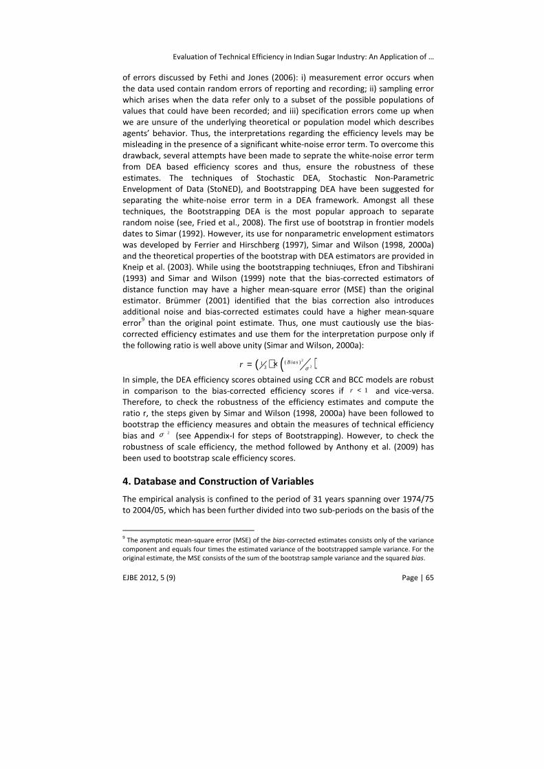
error9 than the original point estimate. Thus, one must cautiously use the bias-

corrected efficiency estimates and use them for the interpretation purpose only if

the following ratio is well above unity (Simar and Wilson, 2000a):

( ) ( )2

2( )1

3B iasr σ= ×

In simple, the DEA efficiency scores obtained using CCR and BCC models are robust

in comparison to the bias-corrected efficiency scores if 1<r and vice-versa.

Therefore, to check the robustness of the efficiency estimates and compute the

ratio r, the steps given by Simar and Wilson (1998, 2000a) have been followed to

bootstrap the efficiency measures and obtain the measures of technical efficiency

bias and 2σ (see Appendix-I for steps of Bootstrapping). However, to check the

robustness of scale efficiency, the method followed by Anthony et al. (2009) has

been used to bootstrap scale efficiency scores.

4. Database and Construction of Variables

The empirical analysis is confined to the period of 31 years spanning over 1974/75

to 2004/05, which has been further divided into two sub-periods on the basis of the

9 The asymptotic mean-square error (MSE) of the bias-corrected estimates consists only of the variance

component and equals four times the estimated variance of the bootstrapped sample variance. For the

original estimate, the MSE consists of the sum of the bootstrap sample variance and the squared bias.


Page | 66 EJBE 2012, 5 (9)

changes in macroeconomic policy governing the Indian economy: i) Pre-reforms

period (1974/75 to 1990/91); and ii) Post-reforms period (1991/92 to 2004/05).

The required data have been provided by the ‘Annual Survey of Industries (ASI)’

wing of Ministry of Statistics and Programme Implementation (MOSPI),

Government of India, on the payment basis.

The foremost requirement for computing technical efficiency levels in the sugar

industry of 12 major sugar producing states is to specify a set of input and output

variables. Our set of variables includes single output and three input variables. A

detailed description of these variables is given in Table 1, in which the gross fixed

capital (GFC) has been adjusted according to the CU levels because “what belongs

to a production function is ‘capital in use’ and not ‘capital in place’ (Solow, 1957)”.

Thus, given the need to estimate a production frontier (or best- practice frontier) in

efficiency analysis of Indian sugar industry, the ‘gross fixed capital (GFC) in place’

has been adjusted to ‘GFC in use’. Moreover, except labour, all the variables have

been deflated by using suitable price indices10

.

Table 1: Description of Variables for Calculating Technical Efficiency Levels

Variable Description

Output:

a) Gross Output Net Output + Depreciation

Inputs:

a) Labour Production Workers + Non-Production Workers

b) Intermediate Inputs Raw Material + Fuel Consumed

c) Gross Fixed Capital in Use CU × (Net Fixed Capital + Depreciation)

Note: See Kumar and Arora (2009b) for capacity Utilization (CU) levels for each state over the study

period and construction of the output and input variables.

Source: Authors’ elaboration

It is worth mentioning that the aforementioned input-output variables obtained for

each individual state are the aggregates of all sugar firms in the state. However, the

number of sugar firms varies widely across the states. With the objective to

minimize the presence of heterogeneity in the data set, we followed Ray (1997),

Kumar (2001), Ray (2002), Kumar (2003) and Kumar and Arora (2009a), and

constructed the state-level input-output quantity data for a ‘representative firm’ in

the industry. For this, the state-level aggregate figures have been divided by the

number of firms operating in the state. The advantage of using data for a

‘representative firm’ is that it imposes fewer restrictions on the production

10

Except labour input (which is measured by number of workers), all other inputs as well as the output

data are reported in the value terms. All nominal values are deflated by appropriate wholesale price

indices to obtain real values. Gross output has been deflated by the price index for sugar and sugar

products; investment has been deflated using implicit deflator for gross fixed capital formation for

registered manufacturing; expenditure on fuels deflated using price index for fuel power and lubricants;

and material expenditure deflated using the general wholesale price index for all commodities.


EJBE 2012, 5 (9) Page | 67

technology11

. In addition, this reduces the effects of random noise due to

measurement errors in inputs and output(s).

5. Empirical Results

As mentioned earlier that the DEA models are deterministic in nature and does not

seprate the white-noise disturbance term from efficiency estimates. Thus, all

deviations from the frontier are assumed to be the consequence of technical

inefficiency in the production process. Thus, the presence of these biases hinders

the robustness of the technical efficiency estimates and also reduces the efficiency

of these estimates. Therefore, testing the significance of the bias is a necessary

condition to draw the appropriate inference from DEA estimates.

To check the significance of the bias, we run the boot.sw98 routine in the Frontier

Efficiency Analysis with R (FEAR) software. The routine follows the steps given by

Simar and Wilson (1998, 2000a) to bootstrap the DEA efficiency scores and report

the bias along with the sample variance of bootstrapped efficiency estimates (2σ ).

Subtracting the bias from the DEA efficiency estimates provides bias-corrected

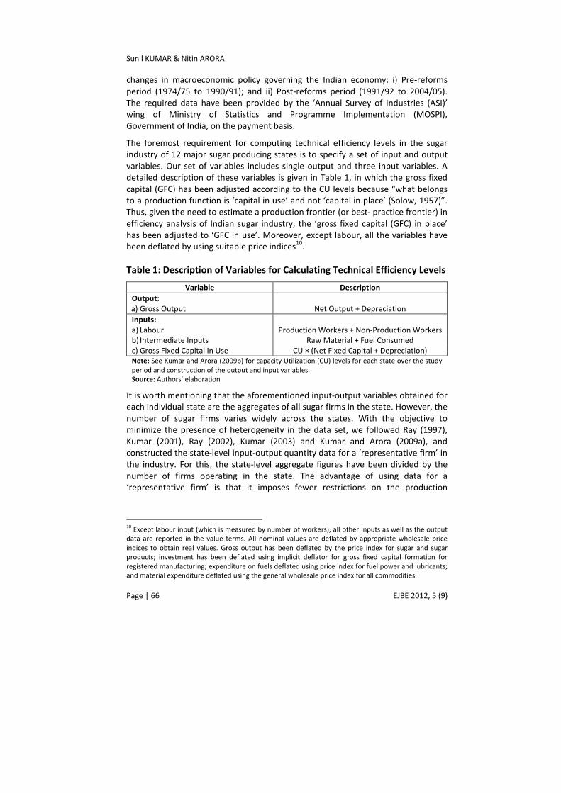
efficiency estimates. However, the bias-corrected estimators should be used only if

the ratio ( ) ( )2

2( )1

3Biasr σ= × is well above unity (Simar and Wilson, 2000a). It

can also be inferred from this statement that if 1r ≥ then DEA scores lack

robustness due to the existence of significant bias, and bias-correction becomes an

obligation.

Table 2 reports the calculated values of r for the three measures of technical

efficiency (i.e., OTE, PTE and SE) and reflects that the calculated values of r

observed to be below unity (i.e., r<1) for entire period and two sub-periods.

Therefore, the efficiency estimates obtained using CCR and BCC models are robust

and worth to be utilized for interpretation purposes. However, the use of bias-

corrected estimates has been ruled out because it will introduce additional noise in

efficiency estimates and increase the mean-square error12

of efficiency estimates.

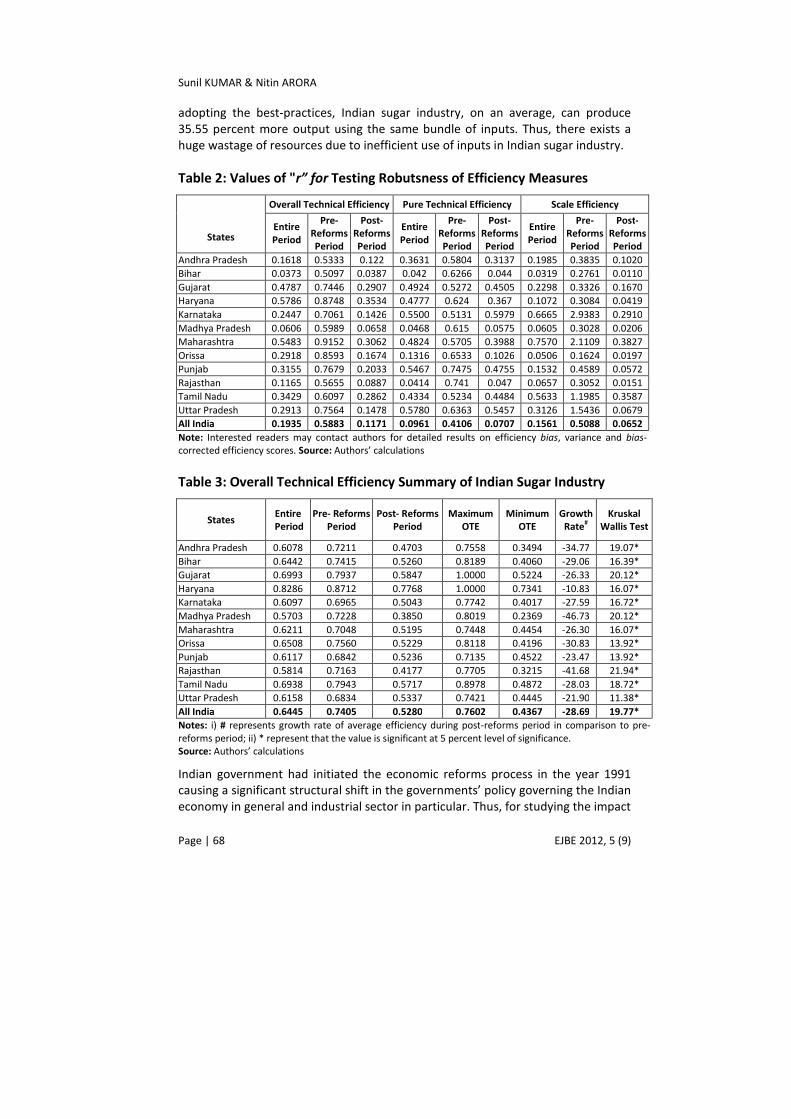
The perusal of Table 3 provides that during the entire study period, the overall

technical efficiency (OTE) score for Indian sugar industry ranges between the

lowest of 43.67 percent to the highest of 73.77 percent, with an average of 64.45

percent. Thus, the level of overall technical inefficiency (OTIE)13

in Indian sugar

industry has been observed to the tune of 35.55 percent. This suggest that by

11

The firm level input-output pairs are feasible, although not individually reported. Therefore, by the

assumption of convexity, the average input-output bundle will always be feasible. The aggregate input-

output bundle will be feasible only under the condition of non-additivity of technology (Ray, 2002). 12

The asymptotic mean-square error (MSE) of the bias-corrected estimates consists only of the variance

component and equals four times the estimated variance of the bootstrapped sample variance. For the

original estimate, the MSE consists of the sum of the bootstrap sample variance and the squared bias. 13

OTIE=1-OTE.


Page | 68 EJBE 2012, 5 (9)

adopting the best-practices, Indian sugar industry, on an average, can produce

35.55 percent more output using the same bundle of inputs. Thus, there exists a

huge wastage of resources due to inefficient use of inputs in Indian sugar industry.

Table 2: Values of "r” for Testing Robutsness of Efficiency Measures

States

Overall Technical Efficiency Pure Technical Efficiency Scale Efficiency

Entire

Period

Pre-

Reforms

Period

Post-

Reforms

Period

Entire

Period

Pre-

Reforms

Period

Post-

Reforms

Period

Entire

Period

Pre-

Reforms

Period

Post-

Reforms

Period

Andhra Pradesh 0.1618 0.5333 0.122 0.3631 0.5804 0.3137 0.1985 0.3835 0.1020

Bihar 0.0373 0.5097 0.0387 0.042 0.6266 0.044 0.0319 0.2761 0.0110

Gujarat 0.4787 0.7446 0.2907 0.4924 0.5272 0.4505 0.2298 0.3326 0.1670

Haryana 0.5786 0.8748 0.3534 0.4777 0.624 0.367 0.1072 0.3084 0.0419

Karnataka 0.2447 0.7061 0.1426 0.5500 0.5131 0.5979 0.6665 2.9383 0.2910

Madhya Pradesh 0.0606 0.5989 0.0658 0.0468 0.615 0.0575 0.0605 0.3028 0.0206

Maharashtra 0.5483 0.9152 0.3062 0.4824 0.5705 0.3988 0.7570 2.1109 0.3827

Orissa 0.2918 0.8593 0.1674 0.1316 0.6533 0.1026 0.0506 0.1624 0.0197

Punjab 0.3155 0.7679 0.2033 0.5467 0.7475 0.4755 0.1532 0.4589 0.0572

Rajasthan 0.1165 0.5655 0.0887 0.0414 0.741 0.047 0.0657 0.3052 0.0151

Tamil Nadu 0.3429 0.6097 0.2862 0.4334 0.5234 0.4484 0.5633 1.1985 0.3587

Uttar Pradesh 0.2913 0.7564 0.1478 0.5780 0.6363 0.5457 0.3126 1.5436 0.0679

All India 0.1935 0.5883 0.1171 0.0961 0.4106 0.0707 0.1561 0.5088 0.0652

Note: Interested readers may contact authors for detailed results on efficiency bias, variance and bias-

corrected efficiency scores. Source: Authors’ calculations

Table 3: Overall Technical Efficiency Summary of Indian Sugar Industry

States Entire

Period

Pre- Reforms

Period

Post- Reforms

Period

Maximum

OTE

Minimum

OTE

Growth

Rate#

Kruskal

Wallis Test

Andhra Pradesh 0.6078 0.7211 0.4703 0.7558 0.3494 -34.77 19.07*

Bihar 0.6442 0.7415 0.5260 0.8189 0.4060 -29.06 16.39*

Gujarat 0.6993 0.7937 0.5847 1.0000 0.5224 -26.33 20.12*

Haryana 0.8286 0.8712 0.7768 1.0000 0.7341 -10.83 16.07*

Karnataka 0.6097 0.6965 0.5043 0.7742 0.4017 -27.59 16.72*

Madhya Pradesh 0.5703 0.7228 0.3850 0.8019 0.2369 -46.73 20.12*

Maharashtra 0.6211 0.7048 0.5195 0.7448 0.4454 -26.30 16.07*

Orissa 0.6508 0.7560 0.5229 0.8118 0.4196 -30.83 13.92*

Punjab 0.6117 0.6842 0.5236 0.7135 0.4522 -23.47 13.92*

Rajasthan 0.5814 0.7163 0.4177 0.7705 0.3215 -41.68 21.94*

Tamil Nadu 0.6938 0.7943 0.5717 0.8978 0.4872 -28.03 18.72*

Uttar Pradesh 0.6158 0.6834 0.5337 0.7421 0.4445 -21.90 11.38*

All India 0.6445 0.7405 0.5280 0.7602 0.4367 -28.69 19.77*

Notes: i) # represents growth rate of average efficiency during post-reforms period in comparison to pre-

reforms period; ii) * represent that the value is significant at 5 percent level of significance.

Source: Authors’ calculations

Indian government had initiated the economic reforms process in the year 1991

causing a significant structural shift in the governments’ policy governing the Indian

economy in general and industrial sector in particular. Thus, for studying the impact


EJBE 2012, 5 (9) Page | 69

of the industrial policy of 1991, the entire study period has been bifurcated into

two sub-periods: i) pre-reforms period from 1974/75 to 1990/91; and ii) post-

reforms period from 1991/92 to 2004/05. The analysis of Table 3 reveals that

during the pre-reforms period, Indian sugar industry has found to be operating

above the efficiency level of 70 percent in each year. However, a precipitous

decline has been noticed during the post-reforms period. To be specific, OTE

declined from the average level of 74.05 percent in the pre-reforms period to 52.80

percent in the post-reforms period indicating a decline in OTE by 28.69 percent in

the post-reforms period. The statistical significance of Kruskall-Wallis test (KW-

Test) statistics support the inference that the decline in OTE during the post-

reforms period is serious enough and hence non-ignorable by all standards.

From Tables 3, it can also be noted that i) for the entire period of study, average

OTE scores range between 0.5703 for Madhya Pradesh and 0.8286 for Haryana.

This indicates that sugar firms in Haryana (Madhya Pradesh) are relatively more

efficient (inefficient) than the firms operating in other states; ii) at the ladder of

efficiency, 2nd and 3rd positions are occupied by the states of Gujarat and Tamil

Nadu with average OTE scores of 0.6993 and 0.6938, respectively; iii) it is

interesting to note that the states of Maharashtra and Uttar Pradesh which are

popularly known as sugar bowls of India positioned almost at the middle of the

efficiency ladder with average OTE scores of 0.6211 and 0.6158, respectively and

thus, ranked at 6th and 7th places; iv) The comparative analysis of average OTE

between two distinct regulatory phases provides that average OTE has declined in

all sugar producing states during the post-reforms period relative to what has been

observed during the pre-reforms period. The statistical significance of the KW H-

Statistics also supports the inference regarding the significant decline in OTE during

the post-reforms period; v) barring the case of Haryana, where average OTE has

declined by about 10.83 percent in the post-reforms period, it has declined by

above and beyond 20 percent in the remaining 11 states; and vi) the decline in OTE

during the post-reforms period is more pronounced in the sugar producing states

of Madhya Pradesh (46.73 percent), Rajasthan (41.68 percent), Andhra Pradesh

(34.77) and Orissa (30.83).

In sum, it can be concluded that there exists substantial inter-state variations in

OTE of Indian sugar industry, and the reforms process has imparted a significant

negative impact on it. On the whole, the analysis reveals the existence of soaring

amount of overall technical inefficiency (OTIE) in the sugar industry of India in

general and sugar industry of 12 major sugar producing states in particular. Thus,

the empirics entail to analyze the causes for such a high level of OTIE in the sugar

industry of India and its sugar producing states.

5.1. Sources of Technical (In) efficiency

To know exactly the causes of OTIE in Indian sugar industry, the measure of OTE

has been decomposed into two non-additive and mutually exclusive components


Page | 70 EJBE 2012, 5 (9)

namely, pure technical efficiency (PTE) and scale efficiency (SE). It is significant to

note that in contrast to OTE measure, the PTE measure is devoid of scale effect.

Therefore, all inefficiency reflected from PTE score directly results from managerial

sub-performance. Keeping aside the scale effect, the PTE score reflects a sort of

managerial efficiency i.e., the ability of management to convert the resources into

output(s) and thus, can be treated as an index of managerial quality. On the other

hand, the SE measure indicates whether the sugar producing state in question is

operating at the most productive scale size (MPSS) or not? The PTE scores have

been obtained by running the BCC model to estimate the cumulative frontier for

each sugar producing state separately.

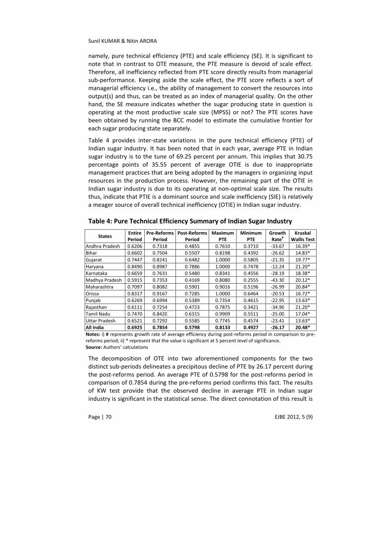
Table 4 provides inter-state variations in the pure technical efficiency (PTE) of

Indian sugar industry. It has been noted that in each year, average PTE in Indian

sugar industry is to the tune of 69.25 percent per annum. This implies that 30.75

percentage points of 35.55 percent of average OTIE is due to inappropriate

management practices that are being adopted by the managers in organizing input

resources in the production process. However, the remaining part of the OTIE in

Indian sugar industry is due to its operating at non-optimal scale size. The results

thus, indicate that PTIE is a dominant source and scale inefficiency (SIE) is relatively

a meager source of overall technical inefficiency (OTIE) in Indian sugar industry.

Table 4: Pure Technical Efficiency Summary of Indian Sugar Industry

States Entire

Period

Pre-Reforms

Period

Post-Reforms

Period

Maximum

PTE

Minimum

PTE

Growth

Rate#

Kruskal

Wallis Test

Andhra Pradesh 0.6206 0.7318 0.4855 0.7610 0.3710 -33.67 16.39*

Bihar 0.6602 0.7504 0.5507 0.8198 0.4392 -26.62 14.83*

Gujarat 0.7447 0.8241 0.6482 1.0000 0.5805 -21.35 19.77*

Haryana 0.8490 0.8987 0.7886 1.0000 0.7478 -12.24 21.20*

Karnataka 0.6659 0.7631 0.5480 0.8341 0.4556 -28.19 18.38*

Madhya Pradesh 0.5915 0.7353 0.4169 0.8080 0.2555 -43.30 20.12*

Maharashtra 0.7097 0.8082 0.5901 0.9016 0.5196 -26.99 20.84*

Orissa 0.8317 0.9167 0.7285 1.0000 0.6464 -20.53 16.72*

Punjab 0.6269 0.6994 0.5389 0.7354 0.4615 -22.95 13.63*

Rajasthan 0.6111 0.7254 0.4723 0.7875 0.3421 -34.90 21.20*

Tamil Nadu 0.7470 0.8420 0.6315 0.9909 0.5511 -25.00 17.04*

Uttar Pradesh 0.6521 0.7292 0.5585 0.7745 0.4574 -23.41 13.63*

All India 0.6925 0.7854 0.5798 0.8133 0.4927 -26.17 20.48*

Notes: i) # represents growth rate of average efficiency during post-reforms period in comparison to pre-



The decomposition of OTE into two aforementioned components for the two

distinct sub-periods delineates a precipitous decline of PTE by 26.17 percent during

the post-reforms period. An average PTE of 0.5798 for the post-reforms period in

comparison of 0.7854 during the pre-reforms period confirms this fact. The results

of KW test provide that the observed decline in average PTE in Indian sugar

industry is significant in the statistical sense. The direct connotation of this result is


EJBE 2012, 5 (9) Page | 71

that the reforms process has worsened the managerial efficiency of the Indian

sugar industry. In addition, PTIE found to be contributing about 90 percent of OTIE

in comparison of 83 percent during the pre-reforms period14

.

The inter-state analysis reveals that barring the sugar industry of Orissa, PTIE

dominates SIE in the remaining 11 sugar producing states. However, in Orissa,

about 48 percent of OTIE is contributed by PTIE and the rest is contributed by SIE.

The analysis regarding the impact of economic reforms on OTE components reveals

that all the sugar producing states have experienced a decline in managerial

efficiency (i.e., PTE) during the post-reforms period. The highest decline has been

observed in Madhya Pradesh (i.e., by 43.30 percent) followed by Rajasthan (i.e.,

34.90 percent) and Andhra Pradesh (i.e., by 33.67 percent). Moreover, barring the

state of Haryana, the sugar industry in the remaining 8 states observed a decline in

average PTE between 20 and 30 percent. Thus, the problem of inapt managerial

practices has become more critical during the post-reforms period.

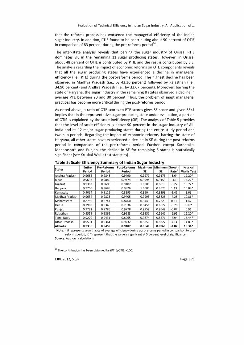
As noted above, a ratio of OTE scores to PTE scores gives SE score and given SE<1

implies that in the representative sugar producing state under evaluation, a portion

of OTIE is explained by the scale inefficiency (SIE). The analysis of Table 5 provides

that the level of scale efficiency is above 90 percent in the sugar industry of All-

India and its 12 major sugar producing states during the entire study period and

two sub-periods. Regarding the impact of economic reforms, barring the state of

Haryana, all other states have experienced a decline in SE during the post-reforms

period in comparison of the pre-reforms period. Further, except Karnataka,

Maharashtra and Punjab, the decline in SE for remaining 8 states is statistically

significant (see Kruskal-Wallis test statistics).

Table 5: Scale Efficiency Summary of Indian Sugar Industry

States Entire

Period

Pre-Reforms

Period

Post-Reforms

Period

Maximum

SE

Minimum

SE

Growth

Rate#

Kruskal

Wallis Test

Andhra Pradesh 0.9686 0.9848 0.9490 0.9979 0.9173 -3.64 12.20*

Bihar 0.9697 0.9880 0.9474 0.9994 0.9159 -4.1 14.22*

Gujarat 0.9382 0.9608 0.9107 1.0000 0.8813 -5.22 18.72*

Haryana 0.9750 0.9688 0.9826 1.0000 0.9523 1.43 10.08*

Karnataka 0.9064 0.9122 0.8993 0.9504 0.8298 -1.41 3.63

Madhya Pradesh 0.9634 0.9823 0.9405 0.9993 0.8825 -4.25 10.86*

Maharashtra 0.8750 0.8741 0.8760 0.9449 0.7223 0.21 1.42

Orissa 0.7980 0.8346 0.7536 0.9451 0.6527 -9.70 8.17*

Punjab 0.9782 0.9785 0.9778 0.9959 0.9549 -0.07 0.91

Rajasthan 0.9559 0.9869 0.9183 0.9951 0.5641 -6.95 12.20*

Tamil Nadu 0.9220 0.9431 0.8965 0.9674 0.8471 -4.94 15.44*

Uttar Pradesh 0.9531 0.9364 0.9732 0.9850 0.8322 3.93 14.83*

All India 0.9336 0.9459 0.9187 0.9648 0.8960 -2.87 10.34*

Note: i) # represents growth rate of average efficiency during post-reforms period in comparison to pre-



14

The contribution has been obtained by (PTIE/OTIE)×100.


Page | 72 EJBE 2012, 5 (9)

The economic literature signifies that scale inefficiency in production operations

does exist despite the firm’s operating either at super-optimal (i.e., at decreasing

returns-to-scale (DRS)) or sub-optimal (i.e., Increasing returns-to-scale)) scales of

production. Thus, the identification of the nature of returns-to-scale becomes

inevitable for each sugar producing state. The nature of scale inefficiencies for a

particular state can be determined by executing an additional DEA program with

the assumption of non-increasing returns-to-scale (NIRS) imposed. By adding the

restriction =

≤∑λ1

1

n

j

j

in DEA model (1), the TE scores assuming NIRS can be

calculated. The calculation of technical efficiency assuming NIRS facilitates the

identification of the nature of returns-to-scale. Let the measure of TE assuming

NIRS be denoted by TENIRS (See, Appendix-II for TENIRS scores). The existence of

increasing or decreasing returns-to-scale can be identified by seeing whether the

TENIRS is equal to the TEVRS: i) if SE<1 and TEVRS=TENIRS then scale inefficiency is

due to decreasing returns-to-scale (DRS) and the representative sugar producing

state has super-optimal scale size; and ii) if SE<1 and TENIRS<TEVRS then scale

inefficiency is due to increasing returns-to-scale (IRS) and the representative sugar

producing state is operating at a sub-optimal size.

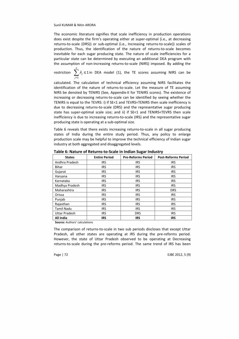
Table 6 reveals that there exists increasing returns-to-scale in all sugar producing

states of India during the entire study period. Thus, any policy to enlarge

production scale may be helpful to improve the technical efficiency of Indian sugar

industry at both aggregated and disaggregated levels.

Table 6: Nature of Returns-to-Scale in Indian Sugar Industry

States Entire Period Pre-Reforms Period Post-Reforms Period

Andhra Pradesh IRS IRS IRS

Bihar IRS IRS IRS

Gujarat IRS IRS IRS

Haryana IRS IRS IRS

Karnataka IRS IRS IRS

Madhya Pradesh IRS IRS IRS

Maharashtra IRS IRS DRS

Orissa IRS IRS IRS

Punjab IRS IRS IRS

Rajasthan IRS IRS IRS

Tamil Nadu IRS IRS IRS

Uttar Pradesh IRS DRS IRS

All India IRS IRS IRS


The comparison of returns-to-scale in two sub periods discloses that except Uttar

Pradesh, all other states are operating at IRS during the pre-reforms period.

However, the state of Uttar Pradesh observed to be operating at Decreasing

returns-to-scale during the pre-reforms period. The same trend of IRS has been


EJBE 2012, 5 (9) Page | 73

noticed among all sugar producing states except the state of Maharashtra during

the post-reforms period. Thus, during the post-reforms period, the state of

Maharashtra has been observed to be operating at DRS. The operation of sugar

producing states at supra-optimal production scale signifies the importance of

downsizing to improve the scale efficiency in general and technical efficiency in

particular.

5.2. Factors Explaining Technical Efficiency

In the above analysis, it has been noted that technical efficiency estimates differ

substantially across Indian states. However, their differences may occur because of

a variety of factors such as access to technology, structural rigidities, differential

incentive systems, level of profitability, etc. We use regression analysis to examine

the influence of environment factors on technical efficiency. As the measures of

technical efficiency are also truncated by the range (0,1], the simple OLS regression

model is inappropriate in the present context. Thus, we make use of the panel data

Truncated regression model to ascertain the impact of environmental variables on

the three measures of efficiency. In the present study, the explanatory variables

that have been used to explain efficiency measures are capital intensity (K/L),

profitability (RETURN) and proportion of non-production employees to total

employees (SKILL). The variable capital intensity (K/L) is defined as ‘gross fixed

capital (GFC) at place’ per employee and used as a measure of relative degree of

mechanization of the production process. High capital intensity signifies a greater

degree of mechanization and expected to facilitate larger operational efficiency.

However, given the already underutilized capacity, an increase in capital per

worker may also affect adversely the productive efficiency. Therefore, capital

intensity variable (K/L) can influence the technical efficiency measures in both ways

i.e., positively or negatively. The variable RETURN is defined as the ratio of

contribution of capital15

to gross fixed capital and used as a proxy for the level of

profitability in an industry. It is hypothesized that profitability has a positive

relationship with the technical efficiency i.e., higher profitability lead to higher

efficiency, and vice-versa. The variable SKILL represents the availability of human

skills and highlights the availability of the trained manpower including supervisory,

administrative and managerial staff. This variable has also been hypothesized to

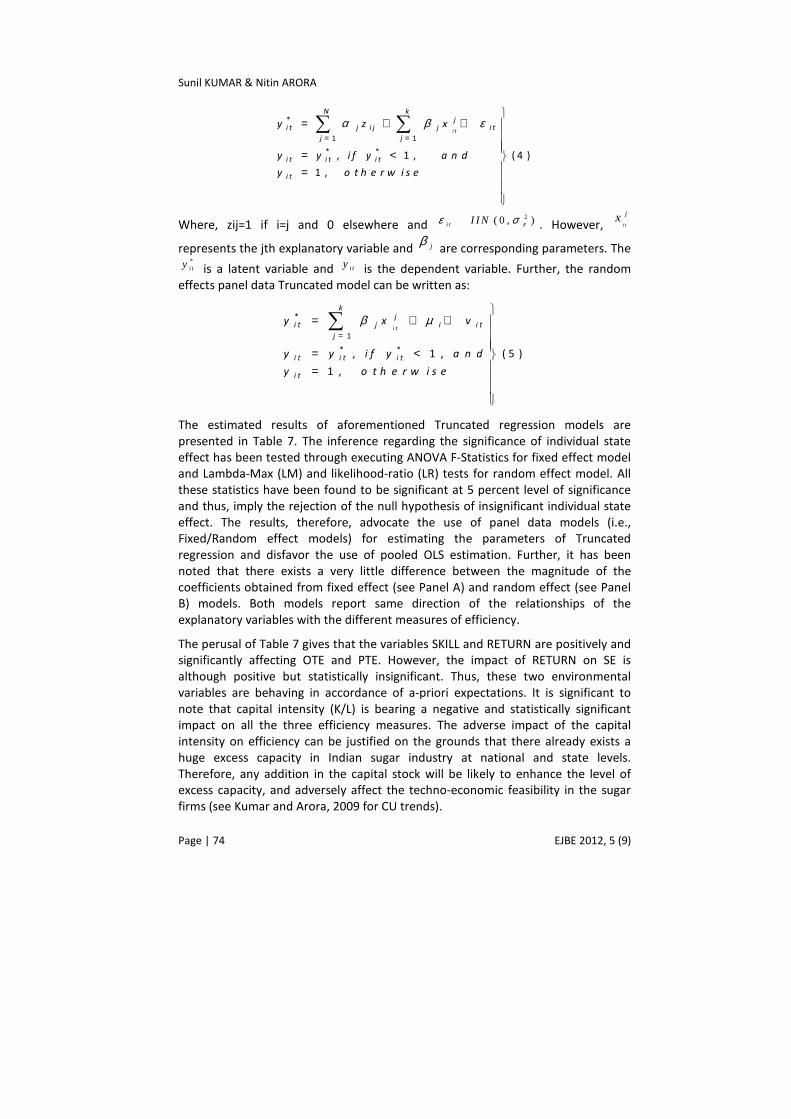
affect technical efficiency positively. The following models (4) and (5) have been

estimated with itx consisting of three variable viz., (K/L), RETURN, and SKILL and

ity i.e., measures of technical efficiency (i.e., OTE, PTE and SE). The one way fixed

effect panel data Truncated model for observation (state) i at time t can be defined

as follows:

15

The contribution of capital has been worked out by subtracting emoluments from the gross value

added.


Page | 74 EJBE 2012, 5 (9)

= =

= + +

= < =

∑ ∑α β ε*

1 1

* *, 1 , ( 4 )

1 ,

i t

N kj

i t j i j j i t

j j

i t i t i t

i t

y z x

y y i f y a n d

y o t h e r w i s e

Where, zij=1 if i=j and 0 elsewhere and 2( 0 , )i t I I N εε σ� . However, i t

jx

represents the jth explanatory variable and jβ are corresponding parameters. The

*i ty is a latent variable and i ty is the dependent variable. Further, the random

effects panel data Truncated model can be written as:

=

= + +

= < =

∑ β µ*

1

* *, 1 , ( 5 )

1 ,

i t

kj

i t j i i t

j

i t i t i t

i t

y x v

y y i f y a n d

y o t h e r w i s e

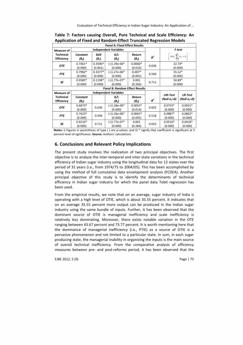
The estimated results of aforementioned Truncated regression models are

presented in Table 7. The inference regarding the significance of individual state

effect has been tested through executing ANOVA F-Statistics for fixed effect model

and Lambda-Max (LM) and likelihood-ratio (LR) tests for random effect model. All

these statistics have been found to be significant at 5 percent level of significance

and thus, imply the rejection of the null hypothesis of insignificant individual state

effect. The results, therefore, advocate the use of panel data models (i.e.,

Fixed/Random effect models) for estimating the parameters of Truncated

regression and disfavor the use of pooled OLS estimation. Further, it has been

noted that there exists a very little difference between the magnitude of the

coefficients obtained from fixed effect (see Panel A) and random effect (see Panel

B) models. Both models report same direction of the relationships of the

explanatory variables with the different measures of efficiency.

The perusal of Table 7 gives that the variables SKILL and RETURN are positively and

significantly affecting OTE and PTE. However, the impact of RETURN on SE is

although positive but statistically insignificant. Thus, these two environmental

variables are behaving in accordance of a-priori expectations. It is significant to

note that capital intensity (K/L) is bearing a negative and statistically significant

impact on all the three efficiency measures. The adverse impact of the capital

intensity on efficiency can be justified on the grounds that there already exists a

huge excess capacity in Indian sugar industry at national and state levels.

Therefore, any addition in the capital stock will be likely to enhance the level of

excess capacity, and adversely affect the techno-economic feasibility in the sugar

firms (see Kumar and Arora, 2009 for CU trends).


EJBE 2012, 5 (9) Page | 75

Table 7: Factors causing Overall, Pure Technical and Scale Efficiency: An

Application of Fixed and Random-Effect Truncated Regression Models Panel A: Fixed Effect Results

Measure of

Technical

Efficiency

Independent Variables

R2

F-test

1

0N

j

j

Null α=

=

∑ Constant

(β0)

Skill

(β1)

K/L

(β2)

Return

(β3)

OTE 0.7461*

(0.000)

0.3596*

(0.001)

(-)1.29e-06*

(0.000)

0.0060*

(0.010) 0.636

22.74*

(0.000)

PTE 0.7982*

(0.000)

0.3377*

(0.000)

(-)1.27e-06*

(0.000)

0.007*

(0.001) 0.594

35.52*

(0.000)

SE 0.9585*

(0.000)

0.1198*

(0.000)

(-)1.77e-07*

(0.000)

0.001

(0.266) 0.711

50.89*

(0.000)

Panel B: Random Effect Results

Measure of

Technical

Efficiency

Independent Variables

R2

LM-Test

(Null σu=0)

LR-Test

(Null σu=0) Constant

(β0)

K/L

(β2)

Return

(β3)

OTE 0.6873*

(0.000) 0.636

(-)1.28e-06*

(0.000)

0.0053*

(0.014) 0.602

0.0753*

(0.000)

0.0931*

(0.000)

PTE 0.7423*

(0.000) 0.594

(-)1.26e-06*

(0.000)

0.0063*

(0.002) 0.518

0.0887*

(0.000)

0.0862*

(0.000)

SE 0.9210*

(0.000) 0.711

(-)1.77e-07*

(0.000)

0.001

(0.284) 0.653

0.0516*

(0.000)

0.0418*

(0.000)

Notes: i) Figures in parenthesis of type ( ) are p-values; and ii) * signify that coefficient is significant at 5

percent level of significance. Source: Authors’ calculations.

6. Conclusions and Relevant Policy Implications

The present study involves the realization of two principal objectives. The first

objective is to analyze the inter-temporal and inter-state variations in the technical

efficiency of Indian sugar industry using the longitudinal data for 12 states over the

period of 31 years (i.e., from 1974/75 to 2004/05). This has been accomplished by

using the method of full cumulative data envelopment analysis (FCDEA). Another

principal objective of this study is to identify the determinants of technical

efficiency in Indian sugar industry for which the panel data Tobit regression has

been used.

From the empirical results, we note that on an average, sugar industry of India is

operating with a high level of OTIE, which is about 35.55 percent. It indicates that

on an average 35.55 percent more output can be produced in the Indian sugar

industry using the same bundle of inputs. Further, it has been observed that the

dominant source of OTIE is managerial inefficiency and scale inefficiency is

relatively less dominating. Moreover, there exists notable variation in the OTE

ranging between 43.67 percent and 73.77 percent. It is worth mentioning here that

the dominance of managerial inefficiency (i.e., PTIE) as a source of OTIE is a

pervasive phenomenon and not limited to a particular state. In sum, in each sugar

producing state, the managerial inability in organizing the inputs is the main source

of overall technical inefficiency. From the comparative analysis of efficiency

measures between pre- and post-reforms period, it has been observed that the


Page | 76 EJBE 2012, 5 (9)

economic reforms process has failed to exert any positive impact on the efficiency

of Indian sugar industry at both national and state levels. This is evident from the

fact that average efficiency of the sugar industry has observed a decline in the post-

reforms period relative to the pre-reforms period.

The panel data Truncated regression analysis aiming to examine the impact of

various explanatory variables on efficiency measures reveals that both availability

of skilled workforce and profitability bear a positive relationship with OTE and PTE.

Further, the capital intensity bears a negative and statistically significant impact on

all three measures of efficiency indicating that higher mechanization does not lead

to increase efficiency of sugar industry. This is perhaps due to already existing

excess capacity in the sugar industry of India.

On the whole, the empirical analysis presents high levels of managerial inefficiency

in major sugar producing states of India. This managerial inefficiency seems to be

the result of excessive government interventions. The government interference in

the production process compels managers to choose a second best alternative

inputs mix rather than choosing the best allocation of resources. As a result, the

managerial inefficiencies remained continue in the production operations of the

sugar firms. Moreover, most of the mills are running with huge losses and thus,

fails to operate efficiently in the company of financial crunch. Most of the times,

sugar firms are observed to be the defaulter even in the payment of sugarcane

arrears. The negative profitability thus, hinders the technical efficiency of sugar

industry. In sum, a policy of decontrolling the sugar industry from the government

control is suggested to improve upon its managerial performance.

References

Anthony, N. R., Kostas, T. and Stavros, T. (2009), “Effects of the European Union Farm Credit

Programs on Efficiency and Productivity of the Greek Livestock Sector: A Stochastic DEA

Application”, Paper Presented at the 8th Annual EEFS Conference, “Current Challenges in the

Global Economy: Prospects and Policy Reforms”, 4-7 June 2009, Warsaw: Faculty of

Economic and Science, University of Warsaw. Available at

<<http://papers.ssrn.com/sol3/papers.cfm?abstract_id=1416747>>

Avkiran, N.K. (2006), “Productivity Analysis in the Services Sector with Data Envelopment

Analysis”, (3rd Ed.), University of Queensland Business School, The University of Queensland,

Australia.

Banker, R. D., Charnes, A., and Cooper, W.W. (1984), “Some Models for Estimating Technical

and Scale Efficiencies in Data Envelopment Analysis”, Management Science, Vol. 30, No. 9,

pp. 1078-1092.

Brümmer, B. (2001), “Estimating Confidence Intervals for Technical Efficiency: The Case of

Private Farms in Slovenia”, European Review of Agricultural Economics, Vol. 28, No. 3, pp.

285-306.

Charnes, A., Cooper, W.W. and Rhodes, E. (1978), “Measuring the Efficiency of Decision

Making Units”, European Journal of Operational Research, Vol. 2, No. 6, pp. 429-444.


EJBE 2012, 5 (9) Page | 77

Charnes, A., Cooper, W.W., Lewin, A.Y. and Seiford, L.M. (eds.) (1994), “Data Envelopment

Analysis: Theory, Methodology and Applications”, Boston USA: Kluwer Academic Publishers.

Efron, B. and Tibshirani, R.J. (1993), “An Introduction to Bootstrap”, London: Chapman and

Hall.

Ferrantino, M.J. and Ferrier, G.D. (1995), “The Technical Efficiency of Vacuum-Pan Sugar

Industry of India: An Application of a Stochastic Frontier Production Function Using Panel

Data”, European Journal of Operational Research, Vol. 80, No. 3, pp. 639-653.

Ferrantino, M.J., and Ferrier, G.D. (1996), “Best-Practice Technology in an Adverse

Environment: The Case of Indian Sugar, 1981-1986”, Journal of Economic Behaviour and

Organization, Vol. 29, No. 3, pp. 493-522.

Ferrantino, M.J., Ferrier, G.D. and Linvill, C.B. (1995), “Organizational Form of Efficiency:

Evidence from Indian Sugar Manufacturing”, Journal of Comparative Economics, Vol. 21, No.

1, pp. 29-53.

Ferrier, G. D. and Hirschberg, J. G. (1995), “Bootstrapping confidence intervals for linear

programming efficiency scores: with an illustration using Italian banking data”, Journal of

Productivity Analysis, Vol. 8, No. 1, pp. 19-33.

Fethi, M.D. and Jones, T.G.W. (2006), “Stochastic Data Envelopment Analysis”, In Avkiran,

N.K. (Eds.), “Productivity Analysis in the Services Sector with Data Envelopment Analysis”,

(3rd ed.), Australlia: University of Queensland Business School, The University of

Queensland.

Fried, H.O., Lovell, C.A.K., and Schmidt, S.S. (2008), “The measurement of Productive

Efficiency and Productivity Growth”, New York USA: Oxford University Press.

Helvoigt, T. and Adams, D.M. (2008), “Data Envelopment Analysis of Technical Efficiency and

Productivity Growth in the US Pacific Northwest Sawmill Industry”, Canadian Journal for

Research, Vol. 38, No. 1, pp. 2553-2565.

ISMA (2008), “Indian Sugar Year Book: 2003-04”, New Delhi India: Indian Sugar Mills

Association.

Jha, R. and Sahni, B.S. (1993), “Efficiency in the Indian Sugar Industry”, Chapter 13,

“Industrial Efficiency: An Indian Perspective”, New Delhi India: South Asia Books.

Kneip, A., Simar, L., and Wilson, P.W. (2003), “Asymptotic for DEA Estimators in Non-

parametric Frontier Models”, Discussion Paper No. 0317, Belgium: Institute de Statistique,

Universitè Catholique de Louvain, Louvain-la-Neuve.

Kumar, S. (2001), Productivity and Factor Substitution: Theory and Analysis, Deep and Deep

Publications Pvt. Ltd., New Delhi.

Kumar, S. (2003), “Inter-Temporal and Inter-State Comparison of Total Factor Productivity in

Indian Manufacturing Sector: an Integrated Growth Accounting Approach”, ArthaVijnana,

Vol. 45, Nos. 3-4, pp 161-184.

Kumar, S. and Arora, N. (2009a), “Does Inspiration or Perspiration Drive Output Growth in

Manufacturing Sector?: An Experience of Indian States”, The Indian Journal of Economics,

Vol. 89, No. 355, pp. 569-598.

Kumar, S. and Arora, N. (2009b), “Analyzing Regional Variations in Capacity Utilization of

Indian Sugar Industry using Non-parametric Frontier Technique”, Eurasian Journal of

Business & Economics, Vol. 2, No. 4, pp. 1-26. Available at: << www.ejbe.org >>


Page | 78 EJBE 2012, 5 (9)

Kumbhakar, S. C. and Lovell, C.A.K. (2003), “Stochastic Frontier Analysis”, (2nd ed.), New

York U.S.A.: Cambridge University Press.

Murty, M.N., Kumar, S. and Paul, M. (2006), “Environmental Regulation, Productive

Efficiency and Cost of Pollution Abatement: A Case Study of the Sugar Industry in India”,

Working Paper Number WP213, New Delhi, India: Institute of Economic Growth, Delhi

University Enclave.

Nighiem, H.S., and Coelli, T. (2002), “The Effect of Incentive Reforms Upon Productivity:

Evidences from the Vietnamese Rice Industry”, Journal of Development Studies, Vol. 39, No.

1, pp. 74-93.

Pandey, A.P. (2007), “Indian Sugar Industry-A Strong Industrial Base for Rural India”, MPRA

Paper No. 6065, Available at: << http://mpra.ub.uni-muenchen.de/6065/ >>

Ray S. (2002), “Economic Reforms and Efficiency of Firms: The Indian Manufacturing Sector

During the Nineties”, Institute of Economic Growth, University of Delhi Enclave, Delhi -

110007, India.

Ray, S.C. (1997), “Regional Variation in Productivity Growth in Indian Manufacturing: A

Nonparametric Analysis”, Journal of Quantitative Economics, Vol. 13, No. 1, pp 73-94.

Sanyal, N., Bhagria, R.P. and Ray, S.C. (2008), “Indian Sugar Industry”, YOJANA, Vol. 52, No. 4,

pp. 13-17.

Seiford, L.M. and Thrall, R.M. (1990), “Recent Developments in DEA: The Mathematical

Programming Approach to Frontier Analysis”, Journal of Econometrics, Vol. 46, No. 1-2, pp.

7-38.

Simar, L. (1992), “Estimating Efficiencies from Frontier Models with Panel Data: A

Comparison of Parametric, Non-Parametric and Semi-Parametric Methods with

Bootstrapping”, Journal of Productivity Analysis, Vol. 3, No. 1, pp. 171-203.

Simar, L. and Wilson, P.W. (1998), “Sensitivity Analysis of Efficiency Scores: How to Bootstrap

in Nonparametric Frontier Models”, Management Science, Vol. 44, No. 1, pp. 49-61.

Simar, L. and Wilson, P.W. (1999), “Estimating and Bootstrapping Malmquist Indices”,

European Journal of Operations Research, Vol. 115, No. 3, pp. 459-471.

Simar, L. and Wilson, P.W. (2000a), “Statistical Inference in Nonparametric Frontier Models:

The State of the Art”, Journal of Productivity Analysis, Vol. 13, No. 1, pp. 49-78.

Simar, L. and Wilson, P.W. (2000b), “A General Methodology for Bootstrapping

Nonparametric Frontier Models”, Journal of Applied Statistics, Vol. 27, No. 6, pp. 779-802.

Singh, N.P., Singh, P. and Pal, S. (2007), “Estimation of Economic Efficiency of Sugar Industry

in Uttar Pradesh: A Frontier Production Function Approach”, Indian Journal of Agriculture

Economics, Vol. 62, No. 2, pp. 232-243.

Singh, S.P. (2006a), “Technical and Scale Efficiencies in the Indian Sugar Mills: An Inter-State

Comparison”, Asian Economic Review, Vol. 48, No. 1, pp. 87-99.

Singh, S.P. (2006b), “Efficiency Measurement of Sugar Mills in Uttar Pradesh”, The ICFAI

Journal of Industrial Economics, Vol. 3, No. 3, pp. 22-38.

Singh, S.P. (2007), “Performance of Sugar Mills in Uttar Pradesh by Ownership, Size and

Location”, Prajnan, Vol. 35, No. 4, pp. 333-360.

Solow, R.M. (1957), “Technical Change and Aggregate Production Function”, Review of

Economics and Statistics, Vol. 39, No. 3, pp. 312-320.

Documents

Evaluation of Technical Efficiency in Indian Sugar ... · PDF filesugar factories and firms with access to sweater cane are more efficient. Further, public-owned firms are found to