Frank M. Meins Enschede, April 2013

Evaluation of spatial scale alternatives for hydrological modelling of the Lake Naivasha basin, Kenya

ii

iii

Evaluation of spatial scale alternatives for hydrological modelling of the Lake Naivasha basin,

Kenya

Master Thesis

by

Frank Martijn Meins

Supervisors: Dr. M.S. Krol (UT, chairman) Dr.ir. M.J. Booij (UT) Dr.ir. P.R. van Oel (ITC) Date: Wednesday, 10 April 2013 Cover photos: different scales of surface runoff representing overland flow, tributary flow and main channel flow.

iv

v

Summary

To understand and predict the effects of anthropogenic interventions on the distribution of water, sediment and pollutants in a drainage basin hydrological models have been, and are still being developed. Most hydrological models use a water balance consisting of a change in water storage in a certain compartment over some time step as a function of rainfall, evapotranspiration, surface runoff and groundwater interactions. The difference between the available models lies in the way these components of the water balance are schematised.

The time period over which processes related to the water balance occur ranges from minutes up to decades; while the areas in which they occur range from several square meters to thousands of square kilometres. Processes that might seem to behave in a certain manner at small scales might behave differently at larger scales, hence information obtained from experiments and observations at a small temporal or spatial scale cannot just be transferred directly to larger scales. Similarly large scale observations cannot directly be used for small scale simulations. This transfer of information from large scales to small scales and vice versa is called downscaling and upscaling respectively and problems associated with it are scale issues, which are studied in this research. The exact definition of scale used in this research is: “a characteristic time or length of a process, observation or model”. This refers to the difference in scale within one analytical dimension (e.g. millimetres, meters or kilometres). The focus is on spatial scale of model implementation. The objective is formulated as follows; “The objective of this study is to evaluate the effect of using different spatial scales for implementing a hydrological model of the upper Lake Naivasha basin, Kenya, on the accuracy of stream flow simulations” In this case ‘accuracy of stream flow simulation’ is defined as the agreement between observed and simulated monthly averaged stream flows (in m3/s).

The study is performed by modelling the hydrology of the Malewa basin, which is a sub-basin of the Lake Naivasha basin, Kenya, and contributes approximately 80% to the surface runoff into Lake Naivasha. The hydrological model that was selected for modelling stream flows in this basin is the Soil Water Assessment Tool (SWAT). The model was considered to be suitable because once the data sets are prepared it is relatively easy to apply different spatial scales. SWAT divides a basin in sub-basins with each their own climate data and channel characteristics. For each of these sub-basins hydrological response units (HRUs) are then defined, which are areas with similar land use, soil and slope characteristics. 7 river gauging stations are available for the Malewa basin which can be used to calibrate the sub-basins. Combining these stations with the SWAT model structure resulted in the application of two types of spatial scales. Firstly three different basin delineations are be applied, with 1, 3 and 7 sub-basins that are generated based on the locations of the river gauging stations to ensure calibration of each sub-basin. Secondly multiple HRUs are applied using only one sub-basin that covers the entire Malewa basin. Additionally, sensitivity of the stream flow simulation to rainfall distribution was tested by applying a homogenous rainfall distribution to the case with 7 sub-basins.

vi

To test accuracy of stream flow simulation the Nash-Sutcliffe Efficiency (NSE) was calculated which explains correlation, bias and relative variability of simulated stream flow values as compared to observed stream flow values. Because of the poor data quality the NSE was calculated at a monthly time scale. When applying the three basin delineations mentioned before, the NSE of the most downstream basin outlet is higher for finer basin delineations. This means that when increasing the number of sub-basins in SWAT the accuracy with which stream flows are simulated increases. It must be noted that this only applies to the simulation of stream flows. Internal flows within the model such as surface runoff, lateral flow and groundwater flow were not included in the calibration procedure and in some cases assumed implausible values. Also, related to this, a number of model parameters adopted implausible values.

When increasing the number of HRUs using only one sub-basin, no trend was observed in the accuracy with which stream flows are simulated. This can be attributed to a combination of two things. Firstly the effect of over-parameterization occurs more prominently when increasing the number of HRUs, because the number of parameters also increases with the number of HRUs while the number of variables used for calibration remains only one (the most downstream outlet). Secondly uncertainty in land use and soil data plays an important role when defining HRUs. Default SWAT parameters were used to represent the different land use types and the soil parameters used were uncertain, this introduces additional uncertainty in the resulting stream flows especially when the number of HRUs is increased. Because of these two things, improvements that were expected to occur when increasing the number of HRUs could not be observed.

The model was found to be sensitive to rainfall and more specifically to the distribution of rainfall. This is because when applying homogenous rainfall to the case with 7 sub-basins, despite having the same rainfall sum, stream flows changed at the most downstream outlet. At sub-basin level rainfall sums did change when applying homogenous rainfall, which affected stream flow as well. In all cases, except for the most downstream one, a certain change in rainfall caused a much larger change in mean stream flow. This means that the model is very sensitive to changes in rainfall.

It is concluded that a basin delineation with more sub-basins results in a more accurate simulation of stream flows when using SWAT. However, issues with data availability in combination with a large number of parameters used during calibration resulted in implausible internal model results despite good stream flow simulation results. This was especially observed when increasing the number of HRUs. Therefore, finer spatial scales of model implementation will improve accuracy of stream flow simulation, but only when data are available at the same spatial scale to ensure an accurate representation of the hydrological processes and to prevent over-parameterization by reducing the number of parameters that need to be calibrated.

vii

Preface

This is the final result of my master thesis project that I conducted to obtain my MSc degree in Civil Engineering and Management. Working on this project was a great experience and I have learned a lot about a variety of topics. Firstly data had to be assimilated which was not an easy task given the fact that, even though most of the data was there, it was not structured into a database and therefore very chaotic. The data also contained a number of gaps, which was one of the reasons of my travel to Kenya. There I learned a lot about how water is managed in Africa and what problems are being faced. By going to Kenya I also learned how to gauge rivers using various methods and of course I was able to enjoy the beauty of Lake Naivasha and its surrounding area.

Collecting data was only the beginning of the process because right after I got back from Kenya I had to find a way to cope with all the gaps in the various data sources and learn to use a hydrological model that I had not used before, the Soil Water Assessment Tool (SWAT). It took a while before the model was up and running, but from all these challenges I have become quite knowledgeable on data analysis, hydrological models and calibration methods which is sure to help me in my future career.

Of course I was not alone in doing this research, I was greatly supported by the employees at WRMA Naivasha, the Naivasha research group at ITC and of course my supervisors from the UT. I would therefore like to thank Pieter van Oel for being my daily supervisor and always being there to discuss any problems I encountered. Also his guidance in Kenya was invaluable because otherwise it would have been much more difficult for me to collect the information I needed. Then I would like to thank Martijn Booij and Maarten Krol for patiently supervising me during the entire period and always providing me with positive and constructive feedback that really helped me to improve my work. I would also like to thank Dominic Wambua for driving me around the Naivasha basin and showing me the locations of all gauging stations. Last but not least I want to thank the members of the Naivasha research group at ITC, Robert Becht, Vincent Odongo, Dawit Mulatu, Francis Muthoni, Jane Ndungu, Rick Hogeboom and Mark Cornelissen for exchanging thoughts about my research and keeping me company during my stay at ITC.

Frank Martijn Meins Enschede, 2013

viii

Table of Contents

1. Introduction...................................................................................................................... 1

1.1. Background ............................................................................................................... 1

1.2. Motivation ................................................................................................................. 1

1.3. Objective and research questions ............................................................................ 5

1.4. Outline....................................................................................................................... 6

2. Study Area ........................................................................................................................ 7

2.1. Geography ................................................................................................................. 7

2.2. Climate ...................................................................................................................... 9

2.3. Hydrology ................................................................................................................ 11

2.4. Water use ................................................................................................................ 12

2.5. Institutional framework .......................................................................................... 13

3. Hydrological Modelling .................................................................................................. 15

3.1. Literature review on hydrological modelling .......................................................... 15

3.2. Model selection ...................................................................................................... 18

3.3. Soil Water Assessment Tool .................................................................................... 19

4. Data & Methods ............................................................................................................. 23

4.1. Data preparation ..................................................................................................... 23

4.2. Scales of model implementation ............................................................................ 36

4.3. Sensitivity analysis .................................................................................................. 40

4.4. Model calibration .................................................................................................... 42

4.5. Model validation & analysis .................................................................................... 43

5. Results ............................................................................................................................ 47

5.1. Rainfall and stream flow interpolation ................................................................... 47

5.2. Sensitivity analysis .................................................................................................. 50

5.3. Basin delineation..................................................................................................... 53

5.4. HRU definition ......................................................................................................... 61

5.5. Rainfall Adjustment................................................................................................. 63

6. Discussion ....................................................................................................................... 65

6.1. Data and model parameters ................................................................................... 65

6.2. Sensitivity analysis and calibration ......................................................................... 67

6.3. Scale issues of model implementation ................................................................... 69

ix

6.4. Water management ................................................................................................ 71

7. Conclusions and recommendations ............................................................................... 73

7.1. Conclusions ............................................................................................................. 73

7.2. Recommendations .................................................................................................. 75

References .............................................................................................................................. 77

x

List of Figures

Figure 1: Characteristic space-time scales of some hydrological processes; Blöschl & Silvaplan (1995) ........................................................................................................................................ 3

Figure 2: Lakes and volcanoes in the East African Rift Valley in Kenya and Ethiopia (Darling et al., 1996) ......................................................................................................................................... 7

Figure 3: Map of the Lake Naivasha basin and its main rivers and mountains .............................. 8

Figure 4: Relation between average annual rainfall and elevation using rain stations within the Lake Naivasha basin .................................................................................................................. 9

Figure 5: Average monthly rainfall of all rain stations in and around the Lake Naivasha basin averaged over a period of 60 years .......................................................................................... 9

Figure 6: Monthly averaged potential evapotranspiration rates measured at different locations within the Lake Naivasha basin............................................................................................... 10

Figure 7: Monthly averaged minimum daily temperatures ......................................................... 10

Figure 8: Monthly averaged maximum daily temperatures ......................................................... 10

Figure 9: Hydrological Cycle of the Lake Naivasha basin; edited from Everard et al. (2002) ....... 11

Figure 10: Water Resources Users Associations (WRUA’s) .......................................................... 14

Figure 11: Soil Storage as modelled in SWAT ............................................................................... 20

Figure 12: Confined (deep) and unconfined (shallow) aquifers (Neitsch et al., 2011) ................. 20

Figure 13: Shallow aquifer as modelled in SWAT ......................................................................... 21

Figure 14: Deep aquifer as modelled in SWAT ............................................................................. 21

Figure 15: Routing Storage as modelled in SWAT ........................................................................ 22

Figure 16: Rainfall interpolation scheme used in this study applied on data from 67 rain stations ................................................................................................................................................. 26

Figure 17: Monthly averaged daily solar radiation ....................................................................... 30

Figure 18: Monthly averaged maximum daily temperatures ....................................................... 30

Figure 19: Monthly averaged minimum daily temperatures ....................................................... 30

Figure 20: Stream flow interpolation scheme used in this study to fill the gaps in the available data series ............................................................................................................................... 32

Figure 21: Stream flow interpolation method, Hughes & Smakhtin (1996) ................................. 34

Figure 22: Lake Naivasha basin (upper left), three main tributaries to Lake Naivasha (lower left), basin delineations using 1, 3 and 7 sub-basins (upper, middle and lower right respectively) ................................................................................................................................................. 38

Figure 23: Comparison of results on different spatial scales ....................................................... 44

Figure 24: Comparison of results using different HRU definitions ............................................... 45

Figure 25: Comparison of results using different rainfall inputs .................................................. 46

Figure 26: Cumulative mass curves of 67 rain stations ................................................................ 47

Figure 27: Percentage of average change in average flow per parameter per basin .................. 51

Figure 28: Percentage of average change in objective function per parameter per basin .......... 52

Figure 29: Nash-Sutcliffe efficiency of simulated stream flows at the 2GB01 outlets for both the calibration and validation periods .......................................................................................... 54

Figure 30: Nash-Sutcliffe efficiency of simulated stream flows at the 2GB05 outlets for both the calibration and validation periods .......................................................................................... 54

xi

Figure 31: Nash-Sutcliffe efficiency of simulated stream flows at the 2GC04 outlets for both the calibration and validation periods .......................................................................................... 54

Figure 32: Relative Volume Error of simulated stream flows at the 2GB01 outlets for both the calibration and validation periods .......................................................................................... 55

Figure 33: Relative Volume Error of simulated stream flows at the 2GB05 outlets for both the calibration and validation periods .......................................................................................... 55

Figure 34: Relative Volume Error of simulated stream flows at the 2GC04 outlets for both the calibration and validation periods .......................................................................................... 55

Figure 35: Hydrograph sub-basin 1.1, validation period 1976-1985 ............................................ 56

Figure 36: Hydrograph sub-basin 3.1, validation period 1976-1985 ............................................ 56

Figure 37: Hydrograph sub-basin 7.1, validation period 1976-1985 ............................................ 57

Figure 38: Observed versus simulated monthly averaged stream flows at the 2GB01 outlet .... 57

Figure 39: Cumulative percentage of basin coverage with increasing land use type, where land use types have been sorted ascending based on the size of the area that they cover ......... 62

Figure 40: Nash-Sutcliffe Efficiency for multiple HRU definitions ................................................ 63

Figure 41: Relative Volume Error for multiple HRU definitions ................................................... 63

Figure 42: Change in average daily stream flow when adjusting rainfall, calculated over the validation period (1976-1985) ................................................................................................ 64

Figure 43: Changes in the shape of Little Gilgil at the 2GA06 RGS, next to the Malewa basin .... 66

xii

List of Tables

Table 1: Water demand in the Lake Naivasha basin (Musota, 2008) ........................................... 13

Table 2: Advantages and disadvantages of 6 different hydrological models when used for studying scale issues ............................................................................................................... 18

Table 3: LULC Reclassification ....................................................................................................... 24

Table 4: Wet/dry probabilities ...................................................................................................... 28

Table 5: Characteristics of river gauging stations in the Naivasha basin ..................................... 31

Table 6: Source stations used for interpolation ........................................................................... 36

Table 7: SWAT Model settings ...................................................................................................... 40

Table 8: SWAT model parameters ................................................................................................ 41

Table 9: Statistics of artificial rain stations (averaged over the period 1960-1985) .................... 48

Table 10: Rainfall sums over the entire basin when using 1, 3 and 7 sub-basins ........................ 48

Table 11: Statistics of interpolated river gauging stations (considered over the period of 1960-2010), stations marked with an asterisk are used in SWAT ................................................... 49

Table 12: RVE and NSE of monthly stream flows for each sub-basin ........................................... 53

Table 13: RVE and NSE of monthly stream flow simulation before and after reversing the calibration period .................................................................................................................... 55

Table 14: Detailed yearly averaged SWAT model output per sub-basin for the calibration period (1962-1975) ............................................................................................................................. 59

Table 15: Optimal parameter values for the 1 and 3 sub-basin delineations .............................. 59

Table 16: Optimal parameter values for the 7 sub-basin delineation .......................................... 60

Table 17: HRU definition of the basin delineations with 1, 3 and 7 sub-basins using one HRU per sub-basin ................................................................................................................................. 61

Table 18: Hydrological response units that were generated ....................................................... 61

Table 19: Effects of changes in rainfall on simulated mean flows over the validation period (1976-1985) ............................................................................................................................. 64

xiii

List of Abbreviations

Abbreviation

Description

ASTER Advanced Space borne Thermal Emission and Reflection Radiometer

DO District Office

EOIA Earth Observation and Integrated Assessment

EPIC Environmental Policy Integrated Climate

ET Evapotranspiration

GDEM Global Digital Elevation Model

GIS Geographic Information System

GLUE Generalized Likelihood Uncertainty Estimation

GR4J Génie Rural à 4 paramètres Journalier

HBV Hydrologiska Byråns Vattenbalansavdelning

HRU Hydrological Response Unit

IWRM Integrated Water Resources Management

KMD Kenya Meteorological Department

KSS Kenya Soil Survey

Landsat MSS Landsat Multi-Spectral Scanner

LH Latin Hypercube

LNGG Lake Naivasha Growers Group

LNRA Lake Naivasha Riparian Association

LULC Land Use and Land Cover

MCMC Monte Carlo Markov Chain

METI Ministry of Economy, Trade and Industry

MSE Mean Squared Error

NASA National Aeronautics and Space Administration

NSE Nash-Sutcliffe Efficiency

OAT One-at-a-Time

PET Potential Evapotranspiration

PSO Particle Swarm Optimization

RGS River Gauging Station

RVE Relative Volume Error

SCE-UA Shuffled Complex Evolution algorithm (University of Arizona)

SCMP Sub-Catchment Management Plan

SUFI Sequential Uncertainty Fitting

SWAT Soil Water Assessment Tool

SWAT CUP Soil Water Assessment Tool Calibration and Uncertainty Program

SWB Simple Water Balance

xiv

SWRRB Simulator for Water Resources in Rural Basins

UTM Universal Transverse Mercator

WAP Water Allocation Plan

WEAP Water Evaluation And Planning System

WRMA Water Resources Management Authority

WRUA Water Resources Users Association

1

1. Introduction

1.1. Background

To understand and predict the effects of anthropogenic interventions on the distribution of water, sediment and pollutants in a drainage basin hydrological models have been, and are still being developed (Feyen & Zambrano, 2011). There are numerous ways to distinguish these models from one another, for example by their spatial resolution or by their model structure. A common distinction is made between empirically based and physically based models, with conceptual models in between, often being a combination of the two (Booij, 2003). Most hydrological models are conceptual and primarily use a water balance consisting of a change in water storage in a certain compartment over some time step as a function of rainfall, evapotranspiration, surface runoff and groundwater interactions. The difference between the models lies in the way these components of the water balance are schematised (e.g. lumped or distributed, stochastic or deterministic, small scale or large scale, daily or monthly time step) (Singh, 1995).

The time period over which processes related to the water balance occur ranges from minutes up to decades; while the areas in which they occur range from several square meters to thousands of square kilometres. Processes that might seem to behave in a certain manner at small scales might behave differently at larger scales, hence information obtained from experiments and observations at a small temporal or spatial scale cannot just be transferred directly to larger scales. Similarly large scale observations cannot directly be used for small scale simulations. For example, a land use map with a resolution of 5 km will be of little use when modelling a basin of 25 km2 that contains multiple different land use types. This transfer of information from large scales to small scales and vice versa is called downscaling and upscaling respectively and problems associated with it are scale issues, which are studied in this research.

Blöschl and Sivapalan (1995) define scale as “a characteristic time or length of a process, observation or model” which refers to the difference in resolution within one analytical dimension. For example, when considering length, available scales would be metres or kilometres. This research explores the issue of scale according to this definition of Blöschl and Sivapalan (1995), with a focus on spatial scale of model implementation. The motivation for this research is elaborated in Section 1.2. It is followed by the formulation of the objective and research questions in Section 1.3 and is concluded with an outline of the remainder of this report in Section 1.4.

1.2. Motivation

In hydrological modelling scales can be grouped into three categories, each category containing both a temporal and spatial component: 1) scales of hydrological processes, 2) scales of observations and, 3) scales of model implementation. These categories are interconnected and ideally the hydrological processes are observed and modelled at the characteristic scale at which they occur (Blöschl & Sivapalan, 1995). Unfortunately this is often not feasible due to physical limitations to observations and computational limitations to hydrological modelling

2

(Beven, 1995), hence scale issues arise. Scale issues are not unique to hydrology but occur in a range of disciplines such as meteorology, morphology and ecology, each using their own terminology. In Section 1.2.1 the terminology related to scale issues and scaling in hydrological modelling as proposed by Blöschl & Silvaplan (1995) is explained and in Section 1.2.2 different studies to the effects on model output of using different spatial scales are discussed.

1.2.1. Definitions

Spatial and temporal scales of hydrological processes are interconnected, as is illustrated in Figure 1. For each process a somewhat linear relation between its characteristic time and spatial scale exists. This linear relation is expressed as the ratio of characteristic spatial scale over characteristic time scale of a process and is referred to as the characteristic velocity of a hydrological process (Blöschl & Sivapalan, 1995). For example, for channel flow this ratio is 1 m/s, implying that a channel of 100 km length operates on a temporal scale in the order of 100,000 seconds (≈27.8 hours). This represents the time required for a disturbance to propagate from the start to the end of the channel. Another scale related property that can be derived from Figure 1 is that each process appears to have its own typical length and time scale on which it becomes dominant. This suggests it is possible to determine which processes should be included in a hydrological modelling exercise by simply considering the size of the catchment. This idea is also supported by Kiersch (2000) who identified a relation between catchment size and the impact of different processes. However, a unified theory of hydrology that combines the processes at their different scales into one framework for modelling catchments of various sizes is yet to be developed (Blöschl, 2001; Vinogradov et al., 2011).

As mentioned before scales in hydrological modelling can be grouped in three categories; scales of processes, observations and model implementation. The first category, scales of hydrological processes, typically consist of three components; 1) lifetime or duration (time or length at which the process occurs), 2) period (time or length over which the process repeats itself) and, 3) correlation length (spatial or temporal range at which the effects of a process affect the system). Some hydrological processes tend to have preferred scales which are referred to as ‘natural scales’. These natural scales are identified by peaks in the spectrum when performing a spectral analysis. The second category in which scale issues can be grouped is observations. This category consists of three components as well; 1) extent or coverage of the dataset, 2) spacing between the samples (resolution) and, 3) integration volume (size) of the sample. Ideally the observational scales equal the process scales. However, this is often not feasible. Two problems may occur; when observations are done at too small scales the processes occur as trends, while when observations are done at too large scales the processes occur as noise. The third category in which scales are defined is model implementation, which can be separated in a spatial and temporal component. Typical spatial scales used when applying a model are local (1 m), hill slope (100 m), catchment (10 km) and regional (100 km) scales; typical temporal scales are event (1 day), seasonal (1 year) and long term (100 years) scales. The most optimal situation occurs when a model is implemented at the scale at which observations are available and that, as stated before, the scale of the observations complies with the scale of the hydrological process that is observed (Blöschl & Sivapalan, 1995).

Scaling can be done in two directions, up and down. Upscaling is the process where a variable observed at a small scale is used to represent a much larger scale. This is often done in

3

two steps; first the small scale variable is distributed over the area and then the distribution is aggregated into one average value for a larger scale. Opposed to this is the process of downscaling where a variable observed at a large scale is disaggregated to a smaller scale. (Blöschl & Sivapalan, 1995).

Figure 1: Characteristic space-time scales of some hydrological processes; Blöschl & Silvaplan (1995)

1.2.2. The scaling problem

Scale issues in hydrological modelling occur most prominently when dividing a drainage basin into sub-basins (Booij, 2005; Tripathi et al., 2006). This type of scale issue is typically a spatial scale issue related to model implementation. Of course this closely relates to temporal scale issues as well as was explained in the previous section and is illustrated by Figure 1. Dividing a basin in sub-basins is done in many hydrological modelling studies, especially when large basins are modelled. The division is based on either flow directions derived from a Digital Elevation Model (DEM), locations of stream flow measurements (for calibration and validation) or administrative boundaries (Beven, 1995; Booij, 2005; Bormann et al., 1999; Vinogradov et al., 2011). The use of sub-basins to model larger basins in general provides a greater level of detail (if data are available at that scale as well), but one must be cautious because model structures that work at small scales cannot just be transferred to larger scales (Merz et al., 2009). These scale issues are summarized with five statements by Vinogradov et al. (2011):

Parameters of macro scale models are generalized parameters at the micro scale.

Relationships and equations are different for different scales.

Equation parameters are different at different scales.

4

A universal scaling methodology, allowing transition from one set of scale parameters to

any other, is highly desired and still undeveloped.

Data are to be collected at the scale required by modelling.

A number of studies have been performed to study these problems each using different approaches and study cases. Goodrich et al. (1997) studied linearity of basin response as a function of scale in semi-arid drainage basins. He found that for semi-arid basins, as opposed to humid basins, runoff response becomes more non-linear with increasing scale, suggesting that different relations do indeed occur at different scales. He contributes this increase in non-linearity of runoff response when increasing scale to ephemeral channel losses and partial storm area coverage. Booij (2005) assessed the effects of using different spatial scales for modelling the River Meuse. He applied the HBV model at three scales, with 118 sub-basins, 15 sub-basins and 1 lumped basin. He concluded that model performance improved when increasing the number of sub-basins. Merz et al. (2009) approached scale issues in a different way as they applied the HBV model to 269 basins of different sizes in Austria and analysed the effects of the basin scale (size in km2) of each individual basin on model performance and model parameters. They concluded that model performance increased when basin scale increased, and that parameters did not change significantly with scale changes though some minor trends at the lower and upper scales were detected. They also noted that when studying scale issues it is important to ensure that the uncertainty in the model output should not be larger than the expected effects of modelling at different scales. A study using SWAT to investigate the influence of spatial scale (basin delineation) on stream flow simulation was performed by Thampi et al. (2010). They modelled an Indian basin (2,362 km2) using two different spatial scales, first they aggregated the basin as one sub-basin and then they modelled only a part of this basin (1,013 km2). They concluded that the model performed reasonably well at both scales but there was a consistent underestimation of peak flows at the larger scale which they contribute to the fact that storm events are modelled less accurately at a coarser scale. Setegn et al. (2008) used SWAT as well to model the Lake Tana basin in Ethiopia. Their study did not focus on scale issues specifically but they did test at which basin delineation their model simulated stream flow most accurately. They concluded that a delineation of 34 sub-basins provided sufficient detail to model the Lake Tana basin (15,096 km2) because an increase in the number of sub-basins did not yield a further improvement in model results. However, only 5 of their 34 sub-basins were gauged and some sub-basins were downstream of these gauges, this indicates a mismatch between the scale of observations and the scale of model implementation.

A different perspective on scale issues is provided by Bergström & Graham (1998) who suggest that there might not be a scale ‘problem’ in hydrological modelling. They modelled the Baltic Sea by dividing it into a large number of smaller basins using HBV. They conclude that the HBV model which was originally designed for small and medium sized basins also performs well at macro-scale basins when considering the total stream flow. They state that for conceptual models it does not matter what scale is used because a large scale basin is simply the sum of a number of small scale basins. While this might be true when looking only at the simulation of the total stream flow, the physical meaning of the calibration parameters and internal model

5

structure might be lost. Stream flow at sub-basin level might not be modelled properly anymore. Tripathi (2006) studied the effects of using different basin delineations of an Indian basin modelled with SWAT. He divided the basin in 1, 12 and 22 sub-basins and concluded that dividing a basin in sub-basins was of little influence on the total runoff values, but the other water balance components varied significantly (up to 60%) when changing the number of sub-basins.

Scale issues are likely to occur most prominently in basins with a high variability of hydrological characteristics, such as tropical regions in Africa, a complication here is that data are often scarce which limits the possible scales at which a model can be implemented (Hughes, 2005). Some studies to the hydrology of such a basin were performed by Lukman (2003) and Muthuwatta (2004) who used the Soil Water Assessment Tool (SWAT) to divide the Lake Naivasha basin, Kenya, in 18 sub-basins. However, they did not assess what the effects would be on model performance when using other delineations. Musota (2008) applied WEAP21 on Lake Naivasha at basin scale, he stated that it was a suitable tool for modelling (and in particular integrated water resources management) because it could adequately simulate the stream flows. This suggests both hydrological modelling approaches, using a semi-distributed and a lumped model might be appropriate. The question remains however which one provides the best model performance, i.e. simulates stream flows most accurately.

This study therefore aims to study the effects of using different spatial scales of model implementation on model performance which is defined as the accuracy with which stream flow is simulated. The Lake Naivasha basin is chosen as a study case because of two reasons; firstly because data, despite containing a number of gaps and errors, are available and can be applied at different scales and secondly, the basin has a very high variability of hydrological characteristics making it suitable for studying scale issues as they will be amplified.

At ITC, Faculty of Geo-Information Science and Earth Observation of the University of Twente, in combination with the University of Nairobi and the University of Egerton an earth observation- and integrated assessment (EOIA) approach to the governance of Lake Naivasha is employed. Whereas former research focussed only on the individual processes, such as ecology and socio-economics in the basin, this project aims to integrate them to gain a better understanding of the interactions between the processes in and around Lake Naivasha (van Oel et al., 2012). One component of this project focuses on modelling the hydrology of the upper basin in relation to changes in land use and land cover (Odongo, 2010). By studying scale issues this research can assist the project by identifying which hydrological modelling scale is most appropriate for modelling this upper basin area.

1.3. Objective and research questions

Based on the motivation in the previous section the following objective is formulated: “The objective of this study is to evaluate the effect of using different spatial scales for implementing a hydrological model of the upper Lake Naivasha basin, Kenya, on the accuracy of stream flow simulations” In this case ‘accuracy of stream flow simulation’ is defined as the agreement between observed and simulated monthly averaged stream flows (in m3/s). The study is performed by modelling

6

the hydrology of the Malewa basin, which is a sub-basin of the Lake Naivasha basin and contributes approximately 80% to the surface runoff into Lake Naivasha. The hydrology is modelled at a number of spatial scales. The choice of spatial scales for model implementation is based on the spatial levels at which stream flows are measured to enable proper calibration for all spatial scales.

The following research questions are formulated to assist in meeting the objective:

What is the effect of using different spatial scales for implementing a hydrological model on the accuracy of stream flow simulations?

What causes differences in accuracy of stream flow simulation at different spatial scales?

To answer these questions a suitable hydrological model that can easily adjust to different spatial scales of model implementation will be selected. Once the model is selected a number of different spatial scales are applied. These scales are chosen based on data availability and model structure. The resulting simulated stream flows for each model scale will be compared with observed values to determine model performance.

1.4. Outline

In Chapter 2 the study area is described with a focus on the geography, climate and hydrology of the basin. In Chapter 3 a literature review on hydrological modelling is given and a suitable model is selected that will be used to study scale issues. In Chapter 4 the methods used to generate and interpolate data series, to calibrate the model and to study the effects of using different scales of model implementation are explained. In Chapter 5 the results of applying these methods are shown and explained. In Chapter 6 these results are discussed and in Chapter 7 the conclusions and recommendations of this research are given.

7

2. Study Area

In this chapter the characteristics of the Lake Naivasha basin are described. In this research only the Malewa sub-basin (which generates 80% of the surface runoff) will be modelled, as will be explained in Chapter 4, but to give a more insightful illustration of the study area the characteristics of the entire Lake Naivasha basin are described here. The focus is on the aspects affecting the hydrology of the basin. First the natural characteristics of the basin are explained. The natural characteristics are grouped in three categories which are geography (Section 2.1), climate (Section 2.2) and hydrology (Section 2.3). Then knowledge on water use is summarized in Section 2.4 and the chapter is concluded by an analysis of the institutional framework in Section 2.5.

2.1. Geography

Figure 2: Lakes and volcanoes in the East African Rift Valley in Kenya and Ethiopia

(Darling et al., 1996)

Lake Naivasha (0o 45’ S, 36o 20’ E) is located at the bottom of the Kenyan Rift Valley at a distance of approximately 80 km North-West of Kenya’s capital, Nairobi. The Kenyan rift valley is part of the larger East African Rift Valley (Figure 2) which is a patchwork of faulted mountain ranges formed during the last 45 million years. Due to this tectonic activity a number of volcanoes occurred that are still present in the area (Bergner et al., 2009).

Lake Naivasha is one of a series of lakes in the East African Rift Valley of which 7 are located in Kenya. From North to South these are Turkana, Baringo, Bogoria, Nakuru, Elmentaita, Naivasha and Magadi. Lake Naivasha is located at an elevation of approximately 1890 m above mean sea level (a.m.s.l.) which makes it the highest of the East African Rift lakes. It is a freshwater shallow basin lake, covering approximately 140 km2 making it the second-largest freshwater lake in Kenya. (Stoof-Leichsenring et al., 2011). In addition to the main lake three separate compartments can be identified: Crescent Lake, Oloiden and Sonachi also known as Crater Lake. Crescent Lake is the deepest compartment located to the West of the main lake with an average depth of 18 meters, while the main lake is more shallow (max. +/- 8 m, this is variable depending on the season and time period considered). At the South lies the smaller Lake Oloiden that has been separated from the main lake for a number of decades. Sonachi is located West of the main lake in a crater and its hydrology is separated from the main lake (Becht et al., 2006).

8

The Lake Naivasha basin is located mostly to the North of the lake and within the basin elevation ranges between 1881 and 3989 m a.m.s.l. These large differences in elevation result in large differences in rainfall regimes (Section 2.2). The basin is partly located on the Kinangop Plateau and is bordered by the Aberdare Mountains to the East, the Mau Escarpment to the West, Mount Longonot to the South, and the Eburru Hills to the North (Figure 3). The Aberdare Mountains and the Mau Escarpment form the two boundaries of the valley reaching to 3989 m and 3048 m respectively making them one of the highest mountain ranges in the valley (Everard et al., 2002). Most water that enters Lake Naivasha is discharged through two rivers, the Malewa and the Gilgil that enter the lake in the North. They originate at an altitude >2500 m a.m.s.l. (Becht & Harper, 2002).

Figure 3: Map of the Lake Naivasha basin and its main rivers and mountains

9

2.2. Climate

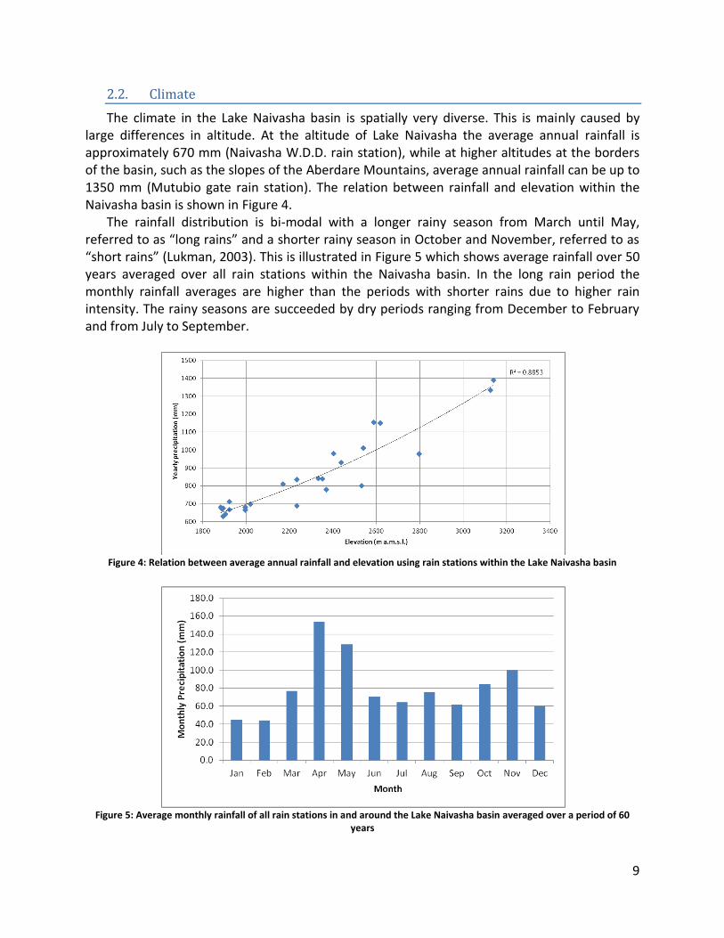
The climate in the Lake Naivasha basin is spatially very diverse. This is mainly caused by large differences in altitude. At the altitude of Lake Naivasha the average annual rainfall is approximately 670 mm (Naivasha W.D.D. rain station), while at higher altitudes at the borders of the basin, such as the slopes of the Aberdare Mountains, average annual rainfall can be up to 1350 mm (Mutubio gate rain station). The relation between rainfall and elevation within the Naivasha basin is shown in Figure 4.

The rainfall distribution is bi-modal with a longer rainy season from March until May, referred to as “long rains” and a shorter rainy season in October and November, referred to as “short rains” (Lukman, 2003). This is illustrated in Figure 5 which shows average rainfall over 50 years averaged over all rain stations within the Naivasha basin. In the long rain period the monthly rainfall averages are higher than the periods with shorter rains due to higher rain intensity. The rainy seasons are succeeded by dry periods ranging from December to February and from July to September.

Figure 4: Relation between average annual rainfall and elevation using rain stations within the Lake Naivasha basin

Figure 5: Average monthly rainfall of all rain stations in and around the Lake Naivasha basin averaged over a period of 60

years

10

The monthly averaged potential evapotranspiration (PET) rates, measured at five locations, are shown in Figure 6. Kalders (1988) measured solar radiation, temperatures, relative humidity and wind speed and used the Penmann-Monteith equation to calculate potential evapotranspiration at Naivasha W.D.D. (close to the Lake, 1940 m a.m.s.l.) and South Kinangop (on the Kinangop plateau, 2591 m a.m.s.l.). Farah (2001) and Mulenga (2002) also measured these variables and used the same equation to calculate PET at Ndabibi (North-West of the lake, 2010 m a.m.s.l.) and Sulmac Farms (South of the lake, ±1900 m a.m.s.l.) respectively. Mmbui (1999) collected pan evaporation data from the Naivasha D.O. station (successor of Naivasha W.D.D.) which was corrected to represent PET. Monthly PET is relatively low from April to July; this is due to cloudiness during and partly after the long rain season (Åse, 1987) and during November because of cloudiness during the short rain season. In general PET is much higher around the lake then at the Kinangop Plateau and near the Aberdares, because temperatures are lower in these regions due to higher elevation.

The climate at Lake Naivasha itself is semi-arid while the climate in the upper parts of the basin is humid (Becht et al., 2006). Mean monthly minimum temperatures in the basin range from 2 C to 12 C, while mean monthly maximum temperatures range from 20 C to 32 C. Average monthly temperatures range from 15.9 C to 17.8 C (De Jong, 2011b). Minimum and maximum daily temperatures averaged over each month are shown in Figure 7 and Figure 8. The stations wea002 and wea025 represent the Naivasha D.O. and North Kinangop stations which are representative for the Lake area and the Kinangop Plateau respectively.

Figure 6: Monthly averaged potential evapotranspiration rates measured at different locations within the Lake Naivasha

basin

Figure 7: Monthly averaged minimum daily temperatures

Figure 8: Monthly averaged maximum daily temperatures

11

2.3. Hydrology

Lake Naivasha has no surface outlet. The water flows into the lake from higher regions via surface flow or ground water flow and either evaporates from the lake or seeps into deeper aquifers connected to the lake that flow towards the South and the North presumably. A first attempt to compute the water balance of Lake Naivasha was done by McCann (1974) who formulated an integral water balance for all East African rift valley lakes. A decade later Åse et al. (1986) studied the balance of lake Naivasha in particular. He formulated it as follows;

Eq. 2.1

In this equation Lt+Δt is the water level of Lake Naivasha after time step Δt, Lt is the water

level water level of the lake at time t, P the amount of rainfall on the lake, I the inflow from the rivers into the lake, E the open water evaporation, ET the evapotranspiration from the vegetation in the lake and S is the seepage to or inflow from the ground water aquifer. The dimensions of all variables are in meters lake level rise. P, I, E, ET and S are summed over time step Δt. This balance defines the key hydrological components that play a role in the water budget of Lake Naivasha. 15 years later Becht & Harper (2002) developed a similar water balance. A difference with the model of Åse et al. (1986) was that it used water volumes instead of converting everything to lake levels, the model was also one of the first to include a dynamic ground water component to model interaction with the aquifer below the lake in time.

According to Gaudet & Melack (1981) 80% of the water that flows into the lake from its basin is surface flow while 20% is subsurface flow, though this sub surface flow component was calculated as the residual term of the water balance and may also contains errors that have not been quantified. It is important to realize that in the Lake Naivasha basin three types of ground water flows can be identified. Firstly the subsurface flows towards the lake mentioned before. Secondly groundwater outflows from the lake towards the deep aquifer and thirdly percolation from the basin directly into the deep aquifer (without reaching the lake).

Deep Aquifer

Sub-surface Water

Figure 9: Hydrological Cycle of the Lake Naivasha basin; edited from Everard et al. (2002)

12

The hydrological cycle as defined by Everard et al. (2002) is schematized in Figure 9. Water evaporated from the Indian Ocean is blown towards the Nyandarua Mountains by the Easterly winds where it precipitates, causing the surface run-off towards Lake Naivasha mentioned previously. A part of the water then evaporates from the lake and moves up the Mau Escarpment where it precipitates and partly flows back into the lake. This flow from the Mau Escarpment is however ephemeral and evaporates before it reaches the lake most of the time (Otiang'a-Owiti & Oswe, 2007).

Lake Naivasha is fed by two main river systems; the Malewa and the Gilgil that enter the lake through a papyrus dominated fringe in the Northern part of the lake. Three smaller river systems that also contribute to the inflow are the Karati, the Nyamithi and the Kwamuya (Everard et al., 2002). The Malewa River contributes approximately 80%, the Gilgil River 10% and the remainder of the surface inflow flows into the lake through the Karati and other seasonal streams (Abiya, 1996). The Malewa and Gilgil rivers are perennial which may suggest rainfall percolating into groundwater tables in the higher regions. These ground water tables can provide the river with water during dry periods, the base flow. Average stream flow volumes of the Malewa and Gilgil rivers are 153 Mm3/year (4.84 m3/s) and 24 Mm3/year (0.76 m3/s) respectively according to Everard et al. (2002). However other studies provide somewhat different values depending on the time period considered (Åse et al., 1986; Becht & Harper, 2002). The total area of the basin is estimated to be 3,376 km2, of which 1,730 km2 is drained by the Malewa system, 527 km2 is drained by the Gilgil, 149 km2 is drained by the Karati and the remaining area is drained by small ephemeral streams that become subsurface flows before reaching the lake (Otiang'a-Owiti & Oswe, 2007). The Malewa and Gilgil systems consist of a number of tributaries feeding the main rivers. Everard et al. (2002) studied these rivers and their tributaries and summarized their characteristics, which can be used for hydrological modelling.

The soils of the Lake Naivasha basin are developed on volcanic ashes caused by the high volcanic activity during the faulting of the Rift Valley (Becht & Harper, 2002). Because of their high pumice content the soils, especially around the lake, are very permeable with a low water holding capacity. This means that water from irrigation activities around the lake seeps into the groundwater aquifer directly and hence no surface flow is caused by irrigation around the lake (Becht et al., 2006). This suggests that most of the surface water flow is caused by rainfall in higher areas and the only flow that is added in the lower regions is base flow.

2.4. Water use

In the early 1980s some farmers around Lake Naivasha started changing their production to floriculture which turned out to be very profitable. This attracted a number of foreign investors and whereas before this development the population around Lake Naivasha consisted mostly of natives, now there were a growing number of non-natives consuming the waters of and around Lake Naivasha for both personal and industrial use (Becht et al., 2006). This growth in agricultural and floricultural activity still continues today (KNBS, 2010) and is characterised by an increase in circle irrigation and green houses directly around the lake.

The most intensive agricultural activities take place directly near the lake, where flower farms are abundant. Two-third of the total water that is abstracted from the Lake Naivasha basin is abstracted there. The remainder is abstracted on the rain fed slopes where less water

13

intensive activities take place such as small-scale subsistence farming, consisting mostly of cash crops such as wheat, maize, potatoes, beans, sunflowers and livestock enterprises (Otiang'a-Owiti & Oswe, 2007). An overview of the water demand is given in Table 1. These estimates are based on a survey performed in 2006 by Rural Focus Ltd. using data from the population census held in 1999 and apply on the total water demand in the lake Naivasha basin.

Table 1: Water demand in the Lake Naivasha basin (Musota, 2008)

Demand type Quantity Units Water requirement [Mm

3/year]

Percentage

Irrigation 5897 Hectares 56.6 71.7%

Livestock 32005 Livestock units 0.5 0.6%

Wildlife 29013 Livestock units 0.9 1.1%

Domestic 812389 People 17.1 21.7%

Industry 3.8 4.8%

Total 78.9 100.0%

Estimates on water abstractions are very uncertain. Abiya (1996) estimated that

approximately 36.9 Mm3/year is abstracted from the Turasha River which is one of the main tributaries of the Malewa River. More recently De Jong (2011b) estimated the total abstraction from all rivers in the basin, based on the extensive Water Abstraction Survey (WAS) held in 2009-2010, to be 28.5 Mm3/year. This is less than the single abstraction from the Turasha River mentioned by Abiya (1996). This could suggest that water abstractions have decreased in more recent years. This is very unlikely because water abstractions are believed to have increased, as a result of increasing population and economic activity. Since different assessment methods were used to obtain these values the difference could be attributed to uncertainty. One specific abstraction stands out (not included in the previous abstraction figures) which is related to a dam that has been built in the Turasha River to supply 65.7 Mm3/year (58.4 Mm3/year according to De Jong (2011b)) to the towns of Nakuru and Gilgil. Unlike the other abstractions this water is diverted outside the basin and no return flow will occur (Abiya, 1996). Including abstractions directly from the lake and groundwater abstractions from the lake aquifer the total water abstraction from the Lake Naivasha basin is estimated to be 101 Mm3/year (De Jong, 2011b). A part of this abstracted water will flow back into the system as return flow, this will cause a delay in surface runoff and stream flows towards the lake.

2.5. Institutional framework

Lake Naivasha is one of Kenya’s five RAMSAR sites (no. 724, 1995) implying it is committed to the Ramsar treaty which defines guidelines for the conservation and sustainable use of natural resources. The lake has a relatively long history of water management. In 1929 the Lake Naivasha Riparian Owners Association (LNROA) was formed by the land owners around Lake Naivasha, this association was responsible for the preservation of the lake and prevented degradation of the lake shores. Later the association became more proactive in maintaining the lake and in 1998 changed its name to the Lake Naivasha Riparian Association (LNRA) as it is still called today. As a reaction to the preservative approach of the LNRA the flower farmers around the Lake also formed an organisation to reflect their commercial interest, the Lake Naivasha

14

Growers Group (LNGG). These two organisations often opposed each other, but due to increased insights that data collection and research have provided many disputes have been settled and both organisations work together to create a sustainable Lake Naivasha (Becht et al., 2006).

The basin around the lake has been divided into twelve management units (plus one additional unit governing all the others) which are named Water Resources Users Associations (WRUAs, Figure 10). The division is mostly based on basin characteristics but also on local administrative settings. The main goal of these associations is to allow for stakeholder participation to enhance water management on a local scale. For each of the associations a Sub-Catchment Management Plan (SCMP) is developed which contains an overview of the characteristics of the basin, the water related problems in it and possible solutions. These plans are based on a coordinating Water Allocation Plan (WAP) which was developed by the Water Resources Management Authority (WRMA); the national body responsible for water management in Kenya which also supervises the WRUAs (WRMA, 2010).

Figure 10: Water Resources Users Associations (WRUA’s)

15

3. Hydrological Modelling

As stated in Chapter 1 this research deals with scale issues in hydrological modelling. In order to study this either a new hydrological model needs to be developed or an already existing model has to be chosen. To make this choice, a review on hydrological modelling is performed first. This review is provided in Section 3.1, a modelling approach is then selected based on an analysis of a number of hydrological models in Section 3.2. In Section 3.3 the selected modelling approach is discussed in more detail.

3.1. Literature review on hydrological modelling

Hydrological models aim to simulate the water balance within a basin which usually comprises a river network or lake. When setting up a model it is common practise to first define the model purpose and specify the modelling context and consequently define which data and prior knowledge are available (Jakeman et al., 2006). Once this is clear a model may be chosen based on the required model features. A large number of hydrological models is available (Singh, 1995) hence developing a new model from scratch is unnecessary laborious in most cases. Regardless of the type of hydrological model that is chosen to model a basin, the quality of the output will largely depend on the quality of the data that is available (Merz et al., 2009). In Africa this often poses a problem, as data are scarce while spatial and temporal variability of the processes are large (Hughes, 2005). When applying an existing model it must be calibrated and validated. To identify which parameters are most sensitive to changes and hence most relevant for calibration a sensitivity analysis is often performed. A number of techniques have been developed for calibration, validation and sensitivity analysis. The most well known methods are shortly explained below.

3.1.1. Sensitivity analysis

A sensitivity analysis or ‘factor screening’ as it is sometimes referred to is often performed to analyse the effects of model inputs, parameters, model equations or initial conditions on a model output. In most environmental models this is done empirically using a computational experiment because these models are too complex to apply classical mathematical analysis (Morris, 1991). A sensitivity analysis aims to support model calibration and uncertainty analysis. It tries to answer the following three questions (Kannan et al., 2007); 1) where data collection efforts should focus; 2) what level of detail should be considered for parameter estimation; and 3) the relative importance of various parameters.

There are a number of techniques developed to perform a sensitivity analysis. The most straightforward one is to vary one parameter at a time within a certain range and determine the effects on the output of the model, the One-factor-at-a-time (OAT) method. The range in which the parameter is varied may be based on physically realistic assumptions derived from literature (Morris, 1991). This type of method is referred to as a univariate or local method.

As opposed to this are multivariate or global methods that consider the change in multiple parameters simultaneously. One such method is the Latin Hypercube (LH) which is a somewhat advanced way of using a Monte Carlo approach with the difference that the random sample is stratified ensuring weighted sampling (Feyen & Zambrano, 2011). It is also possible to combine the LH and OAT method. This combined method divides each parameter in a selected number

16

of bins within a predefined parameter range. From each bin a parameter is selected and a baseline run is performed, then one by one every parameter is changed with a certain percentage or set value and the model is run for each changed parameter to determine model sensitivity for that parameter in that particular point in the parameter space. After all parameters have been changed once, a new parameter sample will be selected from the parameter space. The parameters are selected from bins of which they were not selected before and the same procedure is repeated until all bins have been used once. Using this method interdependency of the parameters (one parameter behaving different for different values of another parameter) is considered in the analysis (Veith & Ghebremichael, 2009).

3.1.2. Calibration and validation

The most sensitive parameters are calibrated by comparing model output at one or multiple locations with measured data. The calibration process is stopped when an objective function does not improve anymore, when parameters do not change anymore or when a time limit is reached. Most calibration methods use an algorithm that selects parameters in an intelligent way and evolve using results of previous iterations in combination with a random component. Calibration methods can be divided into single-objective or multi-objective calibration methods and single or multi-variable calibration methods (Abbaspour, 2011). A multi-objective calibration method uses multiple objective functions to test goodness-of-fit of a simulated variable to its observed data, for example by considering minimization of both the mean squared error and relative volume error simultaneously. Single-objective calibration methods only use one objective function for testing goodness-of-fit. On the other hand a multi-variable calibration considers multiple variables instead of multiple objective functions, for example by using observed stream flows at different locations simultaneously or by using both observed stream flows and observed nutrient flows simultaneously. As opposed to this, a single-variable calibration considers only one variable. Of course combinations using multiple objective functions and multiple variables are possible as well (Feyen & Zambrano, 2011) but will complicate the calibration procedure and increase the required number of iterations. The choice of calibration method to use in a study should be based on the objective that is to be achieved by using the model (Abbaspour, 2011).

Numerous calibration methods exist, ranging from manual single-variable and single-objective calibration to automatic multi-variable and multi-objective calibration. Manual calibration may be applied when only a few parameters are used and when the physical interpretations and ranges of the parameter values are clear. In situations where this is not the case automatic methods are preferred because they can explore large parts of the parameter space much faster. Examples of such automatic methods are Sequential Uncertainty fitting (SUFI), Particle Swarm Optimization (PSO), Generalized Likelihood Uncertainty Estimation (GLUE), Parameter Solution (ParaSol) and Markov Chain Monte Carlo (MCMC) (Abbaspour, 2011; Abbaspour et al., 2004; Beven & Binley, 1992; Hastings, 1970; Kennedy & Eberhart, 1995; van Liew & Veith, 2009). The difference between these methods is the search algorithm that is used to evolve the calibration towards an, often global, optimum. For example ParaSol uses the Shuffled Complex Evolution algorithm (SCE-UA) developed by Duan et al. (1993) while PSO uses neural networks to iterate to an optimum. A disadvantage of automatic calibration schemes is that a lot of computational time may be required to iterate to a desired solution, especially

17

when using spatially distributed models with large numbers of parameters. Also, manual calibration greatly enhances insight of the modeller in the model and the (hydrological) system that is being modelled (Winchell et al., 2010).

A number of statistical tests to evaluate goodness-of-fit are available to use as a calibration objective. Commonly used objective functions are the Nash-Sutcliffe efficiency coefficient (Eq. 3.1) (Nash & Sutcliffe, 1970) and the index of agreement (Eq. 3.2) (Willmott, 1981). Also the relative volume error (Eq. 3.3) may be used as an objective to reduce the error in simulation of total volume. The first two objectives test model performance (goodness-of-fit) by comparing observed (Qobs) and simulated (Qsim) stream flow series over a time period T. The NSE describes the relative magnitude of the residual variance (noise) as compared to the data variance (information). It can range from to 1, where 1 indicates a perfect fit and all values below zero indicate that the mean is a better predictor than the model that is used. The index of agreement includes the variance in the simulated data to overcome differences in means between simulated and observed data. It ranges from 0 to 1 with 0 indicating no agreement at all and 1 indicating a perfect fit. Both NSE and the index of agreement are sensitive to extreme values (Legates & McCabe, 1999). The RVE calculates the excess or shortage of water in the simulation as compared to the observed values, an RVE of 0 implies no water losses while an RVE of 1 or -1 means that the water volume is overestimated or underestimated with 100% respectively (the RVE is often expressed as a percentage).

Eq. 3.1

Eq. 3.2

Eq. 3.3

To validate whether the calibrated parameters represent the characteristics of the basin another observed data set is required other than the one used for calibration. Klemes (1986) developed different schemes for selecting data used for calibration and validation. For a stationary situation two schemes were identified; the split-sample test where a data record is split in two (equal) segments and the proxy-basin test where the model is applied to another basin with similar characteristics, usually for the same time period. In both cases a statistical test, often the same as used during calibration, is applied to determine the accuracy of the simulated output generated during the validation run. If the results are not satisfactory the calibration process may be improved by, for example, allowing for more iterations or if calibration cannot be improved a different model structure may be chosen (Feyen & Zambrano, 2011).

18

3.2. Model selection

A large number of hydrological models has been developed over the last decades, such as the Tank model, Xinanjiang, UBC watershed model, HBV, TOPMODEL, MIKE-SHE, EPIC and many more (Singh, 1995). More recently the Soil Water Assessment Tool (SWAT) (Gassman et al., 2007), the Pitman model (Hughes, 2005), WEAP21 (Yates et al., 2005) and GR4J (Perrin et al., 2003) were developed. Some of these models focus solely on the distribution of water (e.g. HBV, GR4J) while others also include a number of other processes such as nutrients loads and erosion (e.g. SWAT, EPIC). A selection of these models and their application in semi-arid basins are discussed in Appendix A. The models were selected based on their availability and required platform, as well as their usage in equatorial semi-arid basins. The following models are considered; Simple Water Balance model (SWB), HBV hydrological model, Soil Water Assessment Tool (SWAT), Pitman model, Water Evaluation and Planning (WEAP) tool and GR4J. In Table 2 an overview of the advantages and disadvantages of each of the models is given considering the relevance for the study of scale issues.

Table 2: Advantages and disadvantages of 6 different hydrological models when used for studying scale issues

Model Name Advantages Disadvantages

SWB +Easy to understand and implement +Requires almost no computational time +Data at lumped scale is available

-Small scale processes are omitted -No information on the spatial distribution of water in the basin

HBV +The model structure is easy to understand +Requires little computational time +Model is freely available

-Requires manual basin delineation when dividing a larger basins in sub-basin -Interflows between basins are not accounted for

SWAT +Allows for several different basin delineations at different scales +Can easily incorporate changes in land use and land cover +The model is open source and is freely available +Multiple calibration methods are readily available

-Requires more computational time, especially during calibration -Requires more data (suggesting that more assumptions will have to be made)

Pitman +Has been successfully applied to semi-arid African basins before +The model structure is easy to understand

-Requires calibration of 24 parameters -The model is not well known

WEAP21 +Can incorporate the effects of water management decisions easily

-Does not focus on rainfall-runoff modelling -The model is licensed and will be difficult to obtain

GR4J +The model structure is easy to understand +Requires calibration of only 4 parameters +Requires little computational time +The model code is readily available in MATLAB

-Requires manual basin delineation when dividing a larger basins in sub-basin

19

Based on this analysis it appears that SWAT is the most suited model for studying the effects of using different spatial scales of model implementation, because it can most easily deal with changes in basin delineation and allows for incorporation of all data available. HBV, GR4J and the Pitman model each require modifications in order to function properly at each model implementation scale. The SWB model is too simplistic for this study and WEAP21 does not incorporate rainfall-runoff relations in sufficient detail. SWAT can deal more easily with different spatial scales because the input data are already spatially distributed, though some inputs such as rain series will need to be interpolated spatially outside the model to match with different basin delineations. However, these modifications are minor compared to those required by other models. Another advantage of SWAT is that it allows for a much greater range of output variables, such as ground water flows. All in all it can be concluded that out of these models SWAT is the most suited hydrological model for this study to scale issues in hydrological modelling. In the next section a more detailed description of SWAT is given to understand how the model operates and how water flows are calculated.

3.3. Soil Water Assessment Tool

As explained in the previous section the Soil Water Assessment Tool (SWAT) is used to study the effects of using different model scales on stream flows. The version of SWAT used is SWAT2009, and the interface used is ArcSWAT 2009.93.7b which is a plug-in for ArcGIS 9.3.1 SP2. At the start of this study these were the most recent versions. In this section the relevant components of SWAT for modelling hydrology are explained. Each component is visualised and its mass balance is provided. In Appendix B a more detailed explanation of the formulas used to calculate the individual terms is provided. The information in this section and in Appendix B is derived from the three manuals accompanying the ArcSWAT model (Arnold et al., 2011; Neitsch et al., 2011; Winchell et al., 2010).

As stated before SWAT can be divided in two phases; the land phase and the routing phase. In the land phase the runoff (including sediment, nutrients etc.) to the main channel is calculated using either the SCS Curve number method or the Green & Ampt method, in combination with a number of other water flow equations for evaporation, soil and ground water flows. In the routing phase the flows through the channels and between the basins is calculated using either a variable storage method developed by Williams (1969) or the Muskingum method.

In the soil profile a governing water balance equation is used to ensure continuity;

Eq. 3.4

where ΔVsoil is the change in soil water content over time step Δt, Rday is the rainfall that reaches the surface, wirr is the amount of water that infiltrates due to irrigation, Qsurf is the surface runoff, ETa is the evapotranspiration from both soil storage directly and via plant uptake, wseep is the amount of water entering the shallow or deep aquifer from the soil profile and Qlat is the amount of lateral flow through the soil profile. All terms are in mm per time step except for ΔVsoil which is in mm. The soil profile may consist of multiple layers (up to 10) each with their own specific characteristics and thickness. Surface runoff is calculated before

20

infiltration and is directly derived from rainfall and snowmelt of which the latter does not have to be considered in the Naivasha study area.

When water enters the soil profile a part will percolate to the shallow and deep aquifers while another part becomes lateral flow, the remainder stays in the bottom layer of the soil profile. If the bottom soil layer has reached its field capacity the layer above that layer will start to become saturated and so on until the entire soil profile is filled, or until no more water is supplied. In Figure 11 a schematic overview of the soil storage is provided.

Rain (Rday)Irrigation (wirr)

Surface Runoff

(Qsurf)

Soil Storage (max. 10 layers)

Soil Evaporation

(ETa)

Plant Uptake and

Transpiration (ETa)

Lateral Flow

(Qlat)

Seepage

(wseep) Figure 11: Soil Storage as modelled in SWAT

Ground water is stored in the saturated zone below the soil profile. In SWAT ground water

is divided over two aquifers; a shallow aquifer and a deep aquifer which are both fed via the soil storage (Figure 12).

Figure 12: Confined (deep) and unconfined (shallow) aquifers (Neitsch et al., 2011)

21

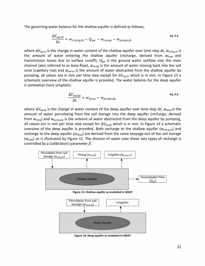
The governing water balance for the shallow aquifer is defined as follows;

Eq. 3.5

where ΔVaq,sh is the change in water content of the shallow aquifer over time step Δt, wrchrg,sh is the amount of water entering the shallow aquifer (recharge, derived from wseep and transmission losses due to surface runoff), Qgw is the ground water outflow into the main channel (also referred to as base flow), wrevap is the amount of water moving back into the soil zone (capillary rise) and wpump is the amount of water abstracted from the shallow aquifer by pumping, all values are in mm per time step except for ΔVaq,sh which is in mm. In Figure 13 a schematic overview of the shallow aquifer is provided. The water balance for the deep aquifer is somewhat more simplistic;

Eq. 3.6

where ΔVaq,dp is the change in water content of the deep aquifer over time step Δt, wdeep is the amount of water percolating from the soil storage into the deep aquifer (recharge, derived from wseep) and wpump,dp is the amount of water abstracted from the deep aquifer by pumping, all values are in mm per time step except for ΔVaq,dp which is in mm. In Figure 14 a schematic overview of the deep aquifer is provided. Both recharge to the shallow aquifer (wrchrg,sh) and recharge to the deep aquifer (wdeep) are derived from the same seepage out of the soil storage (wseep) as is illustrated by Figure 12. The division of water over these two types of recharge is controlled by a (calibration) parameter .

Shallow Aquifer

Irrigation (wpump,sh)Revap (wrevap)

Groundwater Flow

(Qgw)

Percolation from soil

storage (wrchrg,sh)

Figure 13: Shallow aquifer as modelled in SWAT

Deep Aquifer

IrrigationPercolation from soil

storage (wseep,dp)

Figure 14: Deep aquifer as modelled in SWAT

22

The water that is routed through the channel has its own governing water balance as well. It is defined as follows;

Eq. 3.7

where ΔVch is the change in water volume stored in the channel over time step Δt. Vin is the water volume flowing in the reach from either the land phase (surface runoff, lateral flow, return flow) or an upstream basin. Vout is the water volume flowing out of the reach to the next basin. tloss represents transmission losses through the bed of the channel (into the shallow aquifer), Ech represents evaporation losses, div represents either losses or additions due to diversion of the water (f.e. for irrigation) and Vbnk represents water that is returned to the reach via bank storage, all values are in m3 per time step except for ΔVch which is in m3. In Figure 15 schematic overview of the routing storage is provided. In this study Vout is important because this is the quantity on which the model will be calibrated. SWAT also contains a component that includes ponds and reservoirs but this component will not be used and is therefore not discussed here.

The model divides the basin into a specified number of sub-basins by using a DEM and, if available, the locations of gauging stations. The sub-basins each contain their own information on climate; hydrological response units (HRUs); ponds/wetlands and the main channel or reach draining the sub-basin. Hydrological response units are lumped areas within a sub-basin with similar land use, soil properties and slope class. For each HRU the water balances of Eq. 3.4, 3.5 and 3.6 are applied, the water balance of Eq. 3.7 is applied only on the sub-basin scale where the outputs of Eq. 3.4, 3.5 and 3.6 (Surface, lateral and groundwater flows) for each HRU within a sub-basin serve as input for Eq. 3.7 after begin converted from mm to m3 by multiplying with the basin area.

Surface Runoff

Lateral Flow Routing Storage

Irrigation Diversion

Transmission

Losses

Route to next reach or

reservoirReturn Flow

Upstream inflow

Channel

EvaporationBank Storage

Figure 15: Routing Storage as modelled in SWAT

23

4. Data & Methods

In this chapter the methods used to apply the model selected in Chapter 3 and generate the required results are discussed. In Section 4.1 the data used are described along with the interpolation methods used to create complete time series for a number of variables. In Section 4.2 the scales on which the model is implemented are selected and the methods used to perform a sensitivity analysis and calibrate the model are explained in Section 4.3 and 4.4 respectively. In Section 4.5 at the end of this chapter the methods used to validate the model and to study scale issues are explained.

4.1. Data preparation

Research to the physical properties of Lake Naivasha has been performed for over a hundred years; this has resulted in a fair amount of data. Most of these data are related to the direct environment of the lake but also data on the surrounding basin was obtained which is the focus of this research. However, the quality of these data varies in both time and space and contains large gaps which in one way or another need to be accounted for. In this section the available data are described and the methods used to interpolate missing data are explained.

4.1.1. Basin delineation

The first step in this hydrological modelling exercise is delineating the basin by dividing it into sub-basins. This step is important because it determines the scales of model implementation that are used, which is the core of this research. The delineations that are used will be discussed in Section 4.2; in this section the input data that is used for delineation is described. All spatial data are projected onto the UTM Arc 1960 37S projected coordinate system.

4.1.1.1. Global Digital Elevation Model (GDEM)

The “Advanced Spaceborne Thermal Emission and Reflection Radiometer (ASTER) Global Digital Elevation Model (GDEM)” as was developed jointly by the U.S. National Aeronautics and Space Administration (NASA) and Japan’s Ministry of Economy, Trade, and Industry (METI) is freely available on the Internet. This global DEM has a resolution of 30 m and elevation accuracies generally range between 10 and 25 meters root mean square error (ASTER GDEM Validation Team, 2011). The DEM is divided in 1ox1o tiles; the Naivasha basin is fully covered by the 1oS 36oE tile. This tile is used as a basis for basin delineation.

4.1.1.2. Predefined stream flow network

A shape file containing a predefined stream flow network was produced at ITC. To validate this network it was compared with false colour composite ASTER images (LP DAAC, 2011) by using visual inspection. The river network seemed to agree well with the rivers shown on the images, giving confidence in the validity of the network. The network is used where the GDEM does not provide sufficient detail to delineate the streams properly.

24

4.1.1.3. Locations of river gauging stations

The locations of the river gauging stations are one of the criteria used for basin delineation as these are the points at which the model can be calibrated and validated. At ITC a shape file with these locations is available however; this file is both outdated and incomplete, missing a number of stations and containing some stations at wrong locations. Therefore a fieldwork expedition was organised to the Naivasha basin in order to obtain and confirm the coordinates of all river gauging stations in the basin. Also the current status and the data for all these stations were collected as is discussed in Section 4.1.4. A new shape file with the correct locations of the river gauging stations for which data are available was created and projected onto the UTM Arc 1960 37S coordinate system.

4.1.2. Hydrological response units

As explained in the previous chapter SWAT works with HRUs which require three types of input data being land use/land cover data, soil data and slope data. The slopes can be derived from the GDEM mentioned in 4.1.1.1. The land use and soil maps that are used are described in the following two sections.

4.1.2.1. Land use / land cover maps

Land use / land cover (LULC) maps are used to determine which type of vegetation grows in certain areas of the basin. Based on this, hydrological characteristics such as the available canopy storage to store rainfall are derived. A LULC map was produced recently by Odongo (2012), this map is shown in Appendix C. It was produced using a Landsat MSS image of the 21st of December 1973 and represents the period before 1985, when there was no large scale flower farming yet. A vegetation map published in 1976 produced by the British Government's Overseas Surveys was used as a reference for classifying the Landsat MSS in combination with unsupervised classification. During unsupervised classification, 36 classes were first produced which were then aggregated into 8 major classes. Overall accuracy assessment for the produced map was reported as 73%. This was for a large part caused by woodland vegetation which appears sparse on the Landsat MSS image of 1973 whereas on the vegetation map of 1976, the individual/few stands of woodland seem to be generalized with the surrounding dominant land cover. Ignoring the woodland vegetation during accuracy assessment, the accuracy rises to 86% (Odongo, 2012).

Table 3: LULC Reclassification

Original LULC classification

SWAT classification Code

Aquatic Wetlands-mixed WETL

Bushland Range-Brush RNGB

Farmland Agricultural Land-Generic AGRL

Forest Forest-Evergreen FRSE

Grassland Range-Grasses RNGE

Shrubland Pasture PAST

Water Water WATR

Woodland Forest-Mixed FRST

25

The classifications used in this map are converted to similar classifications used in SWAT. It is assumed that the parameters of the land use and land cover types used in SWAT can also represent vegetation in tropical climates (Mango et al., 2011). The descriptions of the LULC classes used by Odongo (2012) are matched with those available in SWAT; the results are shown in Table 3.

4.1.2.2. Soil map

The exploratory soil map produced by the Kenya Soil Survey (Sombroek et al., 1982) was used to identify the soil groups to be used on SWAT. The soil map is available both as hard copy and as a shape file. However, the soil map does not contain all soil parameters in the format required by SWAT (see Appendix D). Therefore Tiruneh (2003) performed a field work expedition in September and October 2003 to identify a number of soil parameters such as hydraulic conductivity (depth up to 120 cm, using the inverse auger-hole method), bulk density and soil composition percentages of sand, silt, clay and rock (Tiruneh, 2003). He translated the results of his fieldwork to the parameters that SWAT required and stored them in an MS Excel file.

To study the issue of scale the same soil map is used for all scales as it is the HRU composition that is changed for each scale and not the soil map itself. To connect the soil shape file to the parameters measured by Tiruneh (2003) first the parameter set is added to the SWAT2009 database file and then a lookup table is defined which connects the soil id in the shape file to the soil name in the edited SWAT2009 database. The parameter values used can be found in Appendix D.2.

4.1.3. Weather data

SWAT uses five different types of weather data; rainfall data, temperature data, solar radiation data, relative humidity data and wind speed data. Relative humidity and wind speed data are not required if the Hargreaves method is used to calculate potential evapotranspiration (Appendix B.2.2). Daily rainfall records are available for longer periods; the other types of data are available for only a few years. To deal with this challenge a weather generator is used to simulate temperatures and solar radiation. Because data on relative humidity and wind speed are not sufficient to calculate the parameters for the weather generator, the Hargreaves method has to be used to calculate PET. The rainfall records contain a number of gaps which have to be interpolated as SWAT requires continuous rainfall series. In the next sections the weather data that are available are discussed and it is explained which methods are used to obtain complete data series that can be used in SWAT.

4.1.3.1. Rainfall

A database containing rainfall data is available from the Kenyan Meteorological Department (KMD). This data was obtained in 2004 and contains data of 65 rain stations. The main data set is up to 1998 but additional rainfall data up to 2010 is available as well. However, most of the data series contain a number of gaps and there is no station, with the exception of Gilgil Kwetu, that has a complete data record for the period of 1960 to 2010. Since SWAT requires complete daily time series for any station that is used, these gaps have to be interpolated. Several interpolation methods are available but in this case considering the reliability of the data a

26

rather simple approach was used. It consists of a daily spatial interpolation in combination with a weather generator for situations where there are not sufficient records on a particular day. A complete overview of the interpolation scheme used is shown in Figure 16. The details of each step are discussed in the following paragraphs.

KMD Daily rainfall data 2004

Assimilate daily rainfall data set

Remove outliers in the daily data and select

time period

Calculate monthly totals and replace totals for

9036002, 9036025, 9036999

Calculate statistics for the weather generator

based on daily data

Use spatial interpolation to fill monthly gaps,

for months with less stations than required by

the threshold, use long-term average to fill

Use a weather generator to generate new

daily data for the periods that could not be

interpolated spatially

Fills the gaps in the original daily data series

with the newly generated data, by replacing

all months with 1 or more missing days

Locations of rainfall stations

GilGil Kwetu, Marula Estate,

Kijabe Farm, North Kinangop

Threshold for maximum daily

rainfall

Formulas to calculate the

statistics

Reliable monthly values of

9036002, 9036025, 9036999

Weather generator script

Spatially interpolate daily rainfall data

Interpolation technique

(inverse distance, threshold

for minimum nr of stations)

Interpolation technique

(inverse distance, threshold

for minimum nr of stations)

Locations of rainfall stations

Calculate elevations of the rainfall stations

and convert all data into .dbf files

GDEM 2011

Locations of rainfall stations

Ensure that the daily interpolated data set

complies with previously developed montly

data set

Figure 16: Rainfall interpolation scheme used in this study applied on data from 67 rain stations

The first step is to collect all the data that is available and assemble them in one matrix

where the rows are daily time steps and the columns are rain stations. In total 67 rain stations

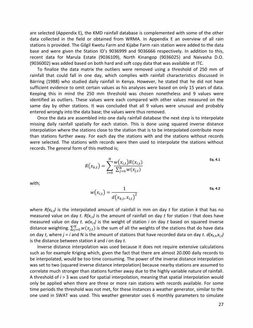
27

are selected (Appendix E), the KMD rainfall database is complemented with some of the other data collected in the field or obtained from WRMA. In Appendix E an overview of all rain stations is provided. The Gilgil Kwetu Farm and Kijabe Farm rain station were added to the data base and were given the Station ID’s 9036999 and 9036666 respectively. In addition to this, recent data for Marula Estate (9036109), North Kinangop (9036025) and Naivasha D.O. (9036002) was added based on both hard and soft copy data that was available at ITC.

To finalize the data matrix the outliers were removed using a threshold of 250 mm of rainfall that could fall in one day, which complies with rainfall characteristics discussed in Bärring (1988) who studied daily rainfall in Kenya. However, he stated that he did not have sufficient evidence to omit certain values as his analyses were based on only 15 years of data. Keeping this in mind the 250 mm threshold was chosen nonetheless and 9 values were identified as outliers. These values were each compared with other values measured on the same day by other stations. It was concluded that all 9 values were unusual and probably entered wrongly into the data base; the values were thus removed.

Once the data are assembled into one daily rainfall database the next step is to interpolate missing daily rainfall spatially for each station. This is done using squared inverse distance interpolation where the stations close to the station that is to be interpolated contribute more than stations further away. For each day the stations with and the stations without records were selected. The stations with records were then used to interpolate the stations without records. The general form of this method is;

Eq. 4.1

with;

Eq. 4.2

where R(xk,t) is the interpolated amount of rainfall in mm on day t for station k that has no measured value on day t. R(xi,t) is the amount of rainfall on day t for station i that does have measured value on day t. w(xi,t) is the weight of station i on day t based on squared inverse distance weighting.

is the sum of all the weights of the stations that do have data

on day t, where j = i and N is the amount of stations that have recorded data on day t. d(xk,t,xi,t) is the distance between station k and i on day t.

Inverse distance interpolation was used because it does not require extensive calculations such as for example Kriging which, given the fact that there are almost 20.000 daily records to be interpolated, would be too time consuming. The power of the inverse distance interpolation was set to two (squared inverse distance interpolation) because nearby stations are assumed to correlate much stronger than stations further away due to the highly variable nature of rainfall. A threshold of i > 3 was used for spatial interpolation, meaning that spatial interpolation would only be applied when there are three or more rain stations with records available. For some time periods the threshold was not met, for these instances a weather generator, similar to the one used in SWAT was used. This weather generator uses 6 monthly parameters to simulate

28

rainfall; these parameters are also required in the SWAT model for other functions so it is convenient to store them as well. These parameters are, two wet/dry probabilities (P(W|W) and P(W|D)), the mean daily rainfall in a month considering only the rainy days (μmon), the standard deviation of the daily rainfall in a month (σmon), the skewness coefficient (gmon) and the number of rainy days (NrR). All parameters have to be calculated for each month (Jan-Dec) and for each station.

The weather generator consists of two components (Neitsch et al., 2011). The first component identifies whether it is a rainy day or not, while the second component identifies how much rain will fall once a day is defined as rainy. To define whether a day is rainy or not a first-order Markov-chain model is used. This model consists of 4 wet/dry probabilities (Table 4) being: a wet day following a dry day P(W|D), a wet day following a wet day P(W|W), a dry day following a wet day P(D|W) = 1 – P(W|W) and a dry day following a dry day P(D|D) = 1 – P(W|D). For each month these probabilities are calculated based on the original data records of a rain station. Then a random number between 0 and 1 is generated, if the generated number is less than the wet dry probability, P(W|D) or P(W|W) depending on the previous day, then a day is defined as wet, otherwise the day is defined as dry and rainfall is set to zero.

Table 4: Wet/dry probabilities

Wet/dry probabilities Wet day at current day Dry day at current day

Wet day at previous day P(W|W) P(D|W)

Dry day at previous day P(W|D) P(D|D)

When the day is wet the amount of rainfall must be defined. This is done by using a skewed

distribution as proposed by Nicks (1974) stated in Neitch (2011). This empirical formula is as follows;

Eq. 4.3

with;

Eq. 4.4

In these formulas Rday is the amount of rainfall on a day defined as wet, μmon is the mean daily rainfall in a month, σmon is the standard deviation of the daily rainfall in a month and gmon is the skewness coefficient. All monthly parameters are obtained for each month by averaging over a period of 51 years (1960-2010) using the original data. The random component is generated by using two random numbers rnd1 and rnd2 which are both between 0 and 1. Since Eq. 4.3 could in some instances generate negative rainfall its lower limit is set to zero. This could give a small underestimation of rainfall but this is compensated for as is explained in the next paragraph.

Based on a preliminary analysis (Appendix E.2) of the data it was found that about 88% of the stations had a higher correlation coefficient (r) when compared with each other for monthly values than for daily values. This implies that missing rainfall data are better estimated on a monthly scale than on a daily scale. This difference in correlation coefficient could be caused by errors in defining the first day of the month, so some series might be shifted one day compared

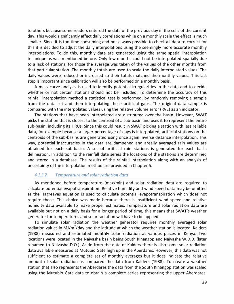
29

to others because some readers entered the data of the previous day in the cells of the current day. This would significantly affect daily correlations while on a monthly scale the effect is much smaller. Since it is too time consuming and not always possible to check all data to correct for this it is decided to adjust the daily interpolations using the seemingly more accurate monthly interpolations. To do this, monthly data are generated using the same spatial interpolation technique as was mentioned before. Only few months could not be interpolated spatially due to a lack of stations, for those the average was taken of the values of the other months from that particular station. The monthly totals are used to scale the daily interpolated values. The daily values were reduced or increased so their totals matched the monthly values. This last step is important since calibration will also be performed on a monthly basis.

A mass curve analysis is used to identify potential irregularities in the data and to decide whether or not certain stations should not be included. To determine the accuracy of this rainfall interpolation method a statistical test is performed, by randomly removing a sample from the data set and then interpolating these artificial gaps. The original data sample is compared with the interpolated values using the relative volume error (RVE) as an indicator.

The stations that have been interpolated are distributed over the basin. However, SWAT picks the station that is closest to the centroid of a sub-basin and uses it to represent the entire sub-basin, including its HRUs. Since this could result in SWAT picking a station with less reliable data, for example because a larger percentage of days is interpolated, artificial stations on the centroids of the sub-basins are generated using once again inverse distance interpolation. This way, potential inaccuracies in the data are dampened and areally averaged rain values are obtained for each sub-basin. A set of artificial rain stations is generated for each basin delineation. In addition to the rainfall data series the locations of the stations are determined and stored in a database. The results of the rainfall interpolation along with an analysis of uncertainty of the interpolation method are provided in Chapter 5.

4.1.3.2. Temperature and solar radiation data

As mentioned before temperature (max/min) and solar radiation data are required to calculate potential evapotranspiration. Relative humidity and wind speed data may be omitted as the Hagreaves equation is used to calculate potential evapotranspiration which does not require those. This choice was made because there is insufficient wind speed and relative humidity data available to make proper estimates. Temperature and solar radiation data are available but not on a daily basis for a longer period of time, this means that SWAT’s weather generator for temperatures and solar radiation will have to be applied.

To simulate solar radiation the weather generator requires monthly averaged solar radiation values in MJ/m2/day and the latitude at which the weather station is located. Kalders (1988) measured and estimated monthly solar radiation at various places in Kenya. Two locations were located in the Naivasha basin being South Kinangop and Naivasha W.D.D. (later renamed to Naivasha D.O.). Aside from the data of Kalders there is also some solar radiation data available measured at Mutubio Gate high up in the Aberdares. However, this data was not sufficient to estimate a complete set of monthly averages but it does indicate the relative amount of solar radiation as compared the data from Kalders (1988). To create a weather station that also represents the Aberdares the data from the South Kinangop station was scaled using the Mutubio Gate data to obtain a complete series representing the upper Aberdares.

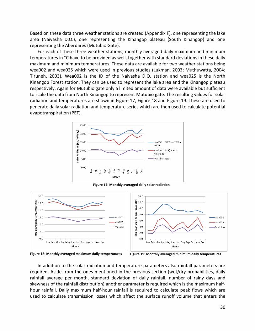
30

Based on these data three weather stations are created (Appendix F), one representing the lake area (Naivasha D.O.), one representing the Kinangop plateau (South Kinangop) and one representing the Aberdares (Mutubio Gate).

For each of these three weather stations, monthly averaged daily maximum and minimum temperatures in C have to be provided as well, together with standard deviations in these daily maximum and minimum temperatures. These data are available for two weather stations being wea002 and wea025 which were used in previous studies (Lukman, 2003; Muthuwatta, 2004; Tiruneh, 2003). Wea002 is the ID of the Naivasha D.O. station and wea025 is the North Kinangop Forest station. They can be used to represent the lake area and the Kinangop plateau respectively. Again for Mutubio gate only a limited amount of data were available but sufficient to scale the data from North Kinangop to represent Mutubio gate. The resulting values for solar radiation and temperatures are shown in Figure 17, Figure 18 and Figure 19. These are used to generate daily solar radiation and temperature series which are then used to calculate potential evapotranspiration (PET).

Figure 17: Monthly averaged daily solar radiation

Figure 18: Monthly averaged maximum daily temperatures

Figure 19: Monthly averaged minimum daily temperatures

In addition to the solar radiation and temperature parameters also rainfall parameters are

required. Aside from the ones mentioned in the previous section (wet/dry probabilities, daily rainfall average per month, standard deviation of daily rainfall, number of rainy days and skewness of the rainfall distribution) another parameter is required which is the maximum half-hour rainfall. Daily maximum half-hour rainfall is required to calculate peak flows which are used to calculate transmission losses which affect the surface runoff volume that enters the

31

main channel (Appendix B). This can be estimated from the daily data as it has not been measured directly. A rather crude assumption was made stating that the maximum rainfall that has occurred in a month has fallen in half an hour and thus equals the maximum half-hour rainfall. For each of the three weather stations one rain station is selected to derive the parameters from, this station is selected based on the location with respect to the weather station and the amount of data that is available. The stations used are Naivasha D.O. (9036002) for the lake area, North Kinangop Forest Station (9036025) for the Kinangop Plateau and Geta Forest station (9038241) for the Aberdares.

4.1.4. Stream flow data

Stream flows are measured by reading water levels from gauging staffs at a number of locations in the basin. These water levels are then converted to stream flows by using rating curves. However, the locations of these gauging staffs in the Naivasha basin were not very well documented and different sources provided different locations. A field work expedition was organised to identify the exact locations of all stations and to obtain all the stream flow data that is available for the stations. Digital data was collected and cross-checked with hard copy data for the period between 1960 and 2010. The gauging locations (stations) that have data for this period are shown in Table 5. The 2GA stations are located in the Gilgil River, the 2GB stations are located in the Malewa and Wanjohi Rivers, the 2GC stations are located in the Turasha River and its tributaries and the 2GD stations in the Karati River.

Table 5: Characteristics of river gauging stations in the Naivasha basin

Station River WRUA X-coordinate Y-coordinate Elevation [m]

2GA01 GILGIL LOWER GILGIL 206516.6 9933672.7 1920

2GA03 GILGIL LOWER GILGIL 204407.4 9945597.2 1996

2GA05 GILGIL LOWER GILGIL - - -

2GA06 LITTLE GILGIL LOWER GILGIL 206495.0 9944747.3 2013

2GB01 MALEWA LOWER MALEWA 210908.0 9938530.8 1951

2GB03 MALEWA UPPER MALEWA 221632.3 9973620.2 2366

2GB04 WANJOHI WANJOHI 219808.8 9969175.2 2334

2GB05 MALEWA LOWER MALEWA 210688.5 9945446.0 1987

2GB0708 MALEWA MIDDLE MALEWA 212081.6 9964640.5 2264

2GC04 TURASHA LOWER MALEWA 212451.6 9946983.4 2000

2GC05 KITIRI MKUNGI KITIRI 228295.2 9939060.7 2408

2GC07 TURASHA UPPER TURASHA 236961.6 9928708.5 2708

2GC10 MUKUNGI MKUNGI KITIRI 225447.7 9942224.9 2419

2GD02 KARATI LANAWRUA 212710.1 9923164.6 1896

2GD07 KARATI KARATI LONGONOT 225922.4 9919576.0 2506

Maps with locations of the gauging stations are shown in Appendix G.1 and G.2. The exact

location of the currently inactive 2GA05 station could not be verified, but it was supposedly located not too far downstream of the current 2GA01 station. 2GB07 and 2GB08 are basically

32

the same stations, but on a slightly different location. In 1997 the 2GB07 station was demolished and in 1998 a new station named 2GB08 was installed approximately 200 meters downstream. These two stations are considered as one station named 2GB0708, which of course does have two different rating curves as is explained below.

The available data consist of water levels measured daily and in some cases sub-daily. In order to be able to use the data for calibration and validation complete daily stream flow series are required. However, due to various circumstances, such as broken staffs and unreliable readers, not all gauging stations contain a complete time series with water levels from 1960 till 2010. To obtain complete daily stream flow series the water levels are converted to stream flows first and then interpolated as is explained in the next two sections. An overview of the steps taken to achieve this is shown in Figure 20.

Q-h Relations Fit the commonly used stage

discharge relation to the data

by using the least square

method to estimate the

parameters

Calculate statistics to

determine accuracy of the

rating curves

Interpolate large gaps using

similar gauging stations

Interpolate small gaps using

linear interpolation in time

Calculate statistics to

determine accuracy of the

interpolation methods

Input Action

Measured gauge heights

Rating Curve Formula

Set with discharges for each

station

Interpolation method and

threshold for small gaps

Interpolation method

Output

Use rating curves to convert

measured gauge heights into

discharges and remove

outliersThreshold for outliers

Insight in accuracy of the

rating curves

Rating Curve Formulas

Formulas to calculate the

statistics

Formulas to calculate the

statistics

Set with discharges for each

station with small gaps

interpolated

Insight in accuracy of the

interpolation

Complete discharges series

for each station

Figure 20: Stream flow interpolation scheme used in this study to fill the gaps in the available data series

33

4.1.4.1. Rating curves

The first step towards obtaining stream flow series (in m3/s) is to convert measured water levels to stream flows. This is done using rating curves which define the characteristic relationship between water level and stream flow. A number of studies has been done to obtain this relationship for some gauging stations in the Naivasha basin (De Jong, 2011a; Podder, 1998), but none of them developed rating curves for all stations consistently. Therefore new rating curves are developed for each station. The rating curves are obtained by using measured stream flows at several points in time for different water levels and then fitting a function through these points. It is common practise to use a function derived from Chezy’s Law for a simple rectangular river profile, which is as follows;

Eq. 4.5

where Q is the stream flow (m3/s), H is the measured water depth (m), H0 is the threshold water depth at which the water starts flowing (m) and C and n are coefficients. Using the least squares method the coefficients C and n as well as the initial water level H0 can be solved using the MS Excel Solver for each river gauging station. The Q-H data used consists of a number of stream flow values with their corresponding water levels measured at random moments in time between 1960 and 2010, where Q is measured using the velocity-area method. By using this method it is assumed that the channel geometry and thus the stage discharge relationship has not changed over time. Also possible effects of hysteresis and backwater curves are not accounted for. Nonetheless for each river gauging station a rating curve was developed based on the data, the results of the rating curve analysis are provided in Appendix G.3.

4.1.4.2. Stream flow interpolation

Once water levels are converted to stream flows they need to be interpolated in order to fill the many gaps that are contained within the data. Outliers in the data are removed first using a specific threshold for each station. Then the data are aggregated to daily values because in some instances there are two measurements per day while SWAT requires only one value per day, this is done by simple averaging. The next step is to interpolate the smaller gaps of less than 7 days; these gaps are interpolated using linear interpolation;

Eq. 4.6

where Qi is the stream flow on day i in gap j, Nj is the length of gap j (number of days), Qstart,j is the stream flow at the start of gap j and Qend,j is the stream flow at the end of gap j.

To interpolate the larger gaps of 7 days or more a method developed by Hughes & Smakhtin (1996) is used. This method aims to interpolate the missing data by using other stations that do have data upstream or downstream in the same river system. In Figure 21 an example of this method is given where one sample is interpolated. First a selection of river gauging stations is made that will act as source stations to interpolate one destination station. For both source

34

stations and destination station flow duration curves (DTQ) are developed. 17 exceedence percentages i (0.01 0.10 1 5 10 20 30 40 50 60 70 80 90 95 99 99.90 99.99) are calculated to avoid the complication of fitting a flow duration curve to the data points. For every day that the destination station contains a gap the stream flow value (QSj) from each of the source stations is selected for that day. Then using logarithmic interpolation the exceedence percentage is determined for each source station (DPj) by interpolating between the two nearest DTQ values;

Eq. 4.7

where the DTQj,i and DTQj,i-1 are the closest stream flow values of the flow duration set of source station j below and above the stream flow value QSj. DPj,i and DPj,i-1 are the exceedence percentages related to DTQj,i and DTQj,i-1. When there is more than one source station (j > 1) the average exceedence percentages is taken;

Eq. 4.8

where n is the number of stations and DPS the average exceedence percentage.

Figure 21: Stream flow interpolation method, Hughes & Smakhtin (1996)

35

To calculate the new stream flow value of the destination station a similar approach is used where the new stream flow value is interpolated using logarithmic interpolation and the flow duration curve of the destination station;

Eq. 4.9

where QDS is the new stream flow value for the destination station and DTQs,i and DTQS,i-1 are the flow duration curve values at DPj,i and DPj,i-1. To complete the interpolation scheme two conditions at the beginning and end of the flow duration curve need to be applied;

Eq. 4.10

as well as two conditions for the cases where stream flow of the source station is zero or where the lower value of the flow duration curve of either the source or destination station is zero;

Eq. 4.11

The selection process of the source stations that are used to interpolate a destination station is supervised. Only stations located in the same river system are used as this will give the best result because they have a physical relation. Water that flows through an upstream station will also flow through a more downstream station (neglecting the effects of abstractions). In Table 6 an overview is provided of which stations were used for interpolation. The 2GC stations are used to interpolate the 2GD stations because the Turasha basin is located next to the Karati basin and is expected to have somewhat similar flow patterns. The same applies to the 2GB (Malewa) stations that are used to interpolate 2GA03 (Gilgil).

A special case is the interpolation of 2GA01 (or 2GA05 as it has been called as well). Because the gauging station might have been moved over time the data are unreliable. Information about this issue is very limited but since it is not far from 2GA03 it was decided to scale the data of 2GA03 to represent 2GA01. This is done by averaging the data that is available for 2GA01 (and 2GA05) and scaling 2GA03 to ensure its average matches the average of 2GA01. However this interpolation introduces much uncertainty and it is seems better not to use this station in any further analyses.

As with the analysis of rainfall data the relative volume error is applied to indicate uncertainty in the data. Results of the analyses are provided in Chapter 5.

36

Table 6: Source stations used for interpolation

Destination Station Source Stations

2GA01 2GA03, 2GA05

2GA03 2GB03, 2GB04, 2GB05, 2GB0708

2GB01 2GB03, 2GB04, 2GB05, 2GB0708, 2GC04, 2GC05, 2GC07, 2GC10

2GB03 2GB04, 2GB05, 2GB0708

2GB04 2GB03, 2GB05, 2GB0708

2GB05 2GB03, 2GB04, 2GB0708

2GB0708 2GB03, 2GB04, 2GB05

2GC04 2GC05, 2GC07, 2GC10

2GC05 2GC04, 2GC07, 2GC10

2GC07 2GC04, 2GC05, 2GC10

2GC10 2GC04, 2GC05, 2GC07

2GD02 2GC04, 2GC05, 2GC07, 2GC10, 2GD07

2GD07 2GC04, 2GC05, 2GC07, 2GC10, 2GD02

4.2. Scales of model implementation

To study scale issues related to model implementation a number of spatial sub-basin configurations is assessed. These sub-basin configurations, also referred to as basin delineations, are selected based on the availability and quality of the stream flow data in order to be able to calibrate the model at each scale. As mentioned before SWAT has two types of spatial components; firstly the basin is divided in sub-basins with each their own weather input and channel characteristics. Secondly each sub-basin contains HRUs which are spatially aggregated units with the same land use, soil type and slope class. For each sub-basin a number of HRUs or just one dominant HRU can be defined based on certain threshold values. Both basin delineation and HRU definition are issues of scale so it is important to select them carefully which is done in the following two sections. The basin delineations used are discussed in Section 4.2.1 and the HRU definition is discussed in Section 4.2.2. In addition to this the model set-up of the remaining model components is discussed in Section 4.2.3.

4.2.1. Basin delineations

A river (or lake) basin is divided in sub-basins to be able to model the basin on a more detailed level. Such a delineation results in an increase in the number of parameters in the model and the number of stream flow outlets required for calibration. The most accurate calibration and validation of the model can be performed when the river gauging stations, containing observed data, are located at the river outlets of the sub-basins. Therefore the available river gauging stations can guide basin delineation. There are three options considered for basin delineation in relation to the number of river gauging stations where a basin refers to the total catchment area that is considered and a sub-basin is part of this overall basin;

37

1) One basin, nr. of RGS = nr. of basins 2) Multiple sub-basins, nr. of RGS = nr. of basins 3) Multiple sub-basins, nr. of RGS < nr. of basins

In the first option there is only one basin with one RGS, this is the coarsest scale of the model, where all the parameters in the entire basin are aggregated and calibrated based on only one outlet. The second option implies the basin is divided in sub-basins and there is an RGS at each sub-basin outlet. This allows for a more detailed calibration where the parameters within each sub-basin can be calibrated separately. As opposed to this is the third option where there are less river gauging stations than sub-basin outlets, which means that not every sub-basin can be calibrated separately but a number of sub-basins would need to be calibrated using only one RGS. This implies that a larger amount of parameters is calibrated based on only one RGS resulting in a decrease of physical credibility of the parameters. Hence option three will not be pursued and it is chosen to use only basin delineations based on the available river gauging stations (option 1 and 2).

As discussed in the previous section a number of river gauging stations is available for the Naivasha basin. The coarsest delineation covers three river basins, being the Gilgil, Malewa and Karati river basins upstream of their most downstream station (2GA01, 2GB01 and 2GD02 respectively). The areas around and South-West of the lake have not been monitored as they contain only a few small ephemeral streams of which most disappear in vault lines before reaching the lake (Becht et al. 2006). The delineated three basins can be seen as separate basins each (Figure 22, lower left corner). However, data quality and availability of the 2GA stations is very low, only the 2GA03 station has a complete and proper data series. This means that for the study to the issue of scale it is not relevant to use the Gilgil basin as it cannot be calibrated and validated properly at different scales. The Karati basin only has two stations which means only two scale cases can be studied at most. Therefore the Karati and Gilgil basins are not used in this study.

The Malewa/Turasha basin on the other hand has a number of proper stations, being 2GB04, 2GB05, 2GB0708, 2GC04, 2GC05 and 2GC07. The most downstream RGS, 2GB01, does not have a very consistent series when compared with both lake levels, rainfall and other RGS, and is therefore replaced by using the sum of the upstream RGS 2GB05 and 2GC04. In total this results in a delineation of 7 sub-basins at the finest scale. On a coarser scale the Malewa (2GB04, 2GB05, 2GB0708) and the Turasha (2GC04, 2GC05, 2GC07) sub-basins can be aggregated in two sub-basins with a smaller third sub-basin based on 2GB01. This 2GB01 sub-basin is modelled as hydrologically inactive in both the delineation with 3 and 7 sub-basins because the outflow always equals the inflow due to the summation of 2GB05 and 2GC04 to obtain stream flows at 2GB01. This assumption is made based on the fact that the area of the 2GB01 sub-basin is less than 4% of the total basin area and since it is located in the relatively dry area around the lake so it will not contribute significantly to the total water balance. The coarsest delineation is the one with only one sub-basin. The delineations are shown in the right part of Figure 22 and have been produced using a GDEM and ArcHydro Tools 1.4. To identify the sub-basins easily each sub-basin in each delineation has been given a number as is also shown in Figure 22.

38

Figure 22: Lake Naivasha basin (upper left), three main tributaries to Lake Naivasha (lower left), basin delineations using

1, 3 and 7 sub-basins (upper, middle and lower right respectively)

It was also considered to delineate the basin using the WRUA boundaries. However, this is

not feasible from a hydrological point of view because some of the WRUA boundaries cross the natural basin boundaries. This would imply generating a large number of smaller basins within each WRUA in order to meet the requirement of matching hydrological boundaries with the WRUA boundaries. At such a detailed spatial scale no stream flow series are available. Therefore it would not be possible to calibrate and validate each sub-basin individually making it not suited for this study to scale issues in hydrological modelling.

39

4.2.2. HRU Definition

Once the basin delineation is determined the amount and composition of HRUs in each sub-basin needs to be defined. In total there are 7 land use classes, 12 soil classes and 2 slope classes (using an 80% threshold) identified. This means that in the overall basin a theoretical maximum number of 168 HRUs can be defined, though in practice this is only 96 because not every land use is covered by all soil and slope classes. Since a number of parameters are HRU dependent this would result in hundreds of parameters per sub-basin. Some of these parameters can be measured either directly or indirectly, so if a fieldwork campaign is carried out to measure the parameters with sufficient accuracy then it could be considered to use this many HRUs. But even then there would still be a number of non-physically based parameters (such as soil evaporation and plant uptake coefficients) that have to be calibrated. Currently, only a limited number of the required parameters are actually measured or estimated, which means that a large number of parameters needs to be calibrated. But since there is only one river gauging station at the downstream end of a sub-basin the physical credibility of the parameters becomes disputable when using this many HRUs and hence it seems more efficient to simply use one HRU per sub-basin. Therefore one HRU per sub-basin is used when calibrating the model at each spatial scale, consisting only of the dominant land use, soil and slope classes. In Section 4.5 a method to study the importance of HRU definition in relation to basin delineation is discussed.

4.2.3. Model set-up

Once the basin delineation, HRUs and weather data are loaded there are still a number of settings in the model that that have to be applied before running the model. The initial model settings that are used are discussed in this section.

First of all due to data limitations the Hargreaves method is used to calculate potential evapotranspiration as was explained before. Daily maximum half-hour rainfall is calculated using one representative value for every day in a month as opposed to using a triangular distribution which could produce unrealistic values due to a random component. To calculate surface runoff the Curve Number method is used because the alternative method (Green-Ampt) requires sub-daily rainfall data which is not available. The daily curve number is determined by adjusting the curve number for average soil moisture conditions (CN2). This can be done in two ways, firstly as a function of the soil moisture and secondly as a function of plant evapotranspiration. Because the plant evapotranspiration is assumed to be less reliable due to high uncertainty in the weather data (temperatures and solar radiation) it is chosen to let the Curve Number be adjusted as a function of soil moisture. The routing method used is the variable storage method because the alternative, Muskingum method, requires additional calibration parameters which cannot be estimated based on measurements. Those parameters would have to be included in the calibration process increasing calibration time and adding to over-parameterization. An overview of the settings related to the methods mentioned above is summarized in Table 7.

A number of components are not considered and are switched off. These are: stream water quality, channel degradation, crack flow, urban land cover, elevation bands, climate change increase and irrigation. The time period used ranges from 1960 to 1985 as this is also the period

40

for which the land use map is assumed valid. A two years warm up period is defined to initialise the model which means that the model will run two years before producing any output and calibration is started. Water use is not modelled because during the selected time period there is only small scale water use which does not significantly affect the hydrology of the basin. This small scale water use is indirectly included in the model by calibration of the parameters, for example simulated evaporation rates may be slightly higher than actual evaporation rates to compensate for small scale water use. For the initial run and sensitivity analysis the default SWAT parameters are used together with the soil parameters shown in Appendix D and the settings shown in Table 7.

Table 7: SWAT Model settings

Parameter Definition Setting

IPET Potential evaporation calculation method Hargreaves method (IPET = 2)

IEVENT Surface-runoff-routing method Curve Number method (IEVENT = 0)

ICN Daily Curve Number method Soil moisture based (ICN = 0)

IRTE Flow routing method Variable Storage method (IRTE = 0)

ISED_DET Method used to generate daily maximum half-hour rainfall

Monthly max. HH rainfall value (ISED_DET = 1)

4.3. Sensitivity analysis

The sensitivity analysis tool included in ArcSWAT and developed by Van Griensven (2005) is used to execute the sensitivity analysis. The tool uses the One-factor-At-a-Time Latin Hypercube method (OAT-LH) to select the parameter samples. During sensitivity analysis, SWAT runs (p+1)*m times, where p is the number of parameters being evaluated and m is the number of LH loops and 1 represents the baseline run for each LH loop. At the start of the analysis each parameter range is divided in m segments of equal size. For each loop, a set of parameter values is selected such that a unique area of the parameter space is sampled. This is done by ensuring that each segment of the parameter range can only be used once for sampling. That set of parameter values is used to run a baseline simulation for that unique area. Then, using one-at-a-time (OAT), one by one each parameter is selected, and its value is changed from the baseline with a predefined percentage and the model is run to assess the effect of that particular parameter change on either average stream flow or an objective function. After all parameters have been varied once, the LH algorithm locates a new sampling area by changing all the parameters (van Liew & Veith, 2009).

A total of 27 parameters that relate to the calculation of stream flow can be analyzed using the tool as well as a number of parameters related to sedimentation and water quality but those will not be used. Of these 27 parameters 6 relate to snowfall/snowmelt and will not be considered as there is no snowfall or snowmelt in the Lake Naivasha basin. One parameter is related to water management operations which are not included and will therefore not be considered either. An overview of the 20 remaining parameters, with their range and their function is given in Table 8. The parameter ranges represent the minimum and maximum value for each parameter that is still physically feasible, though in some extreme cases the ranges may be extended (Neitsch et al., 2011). In this study the default ranges are used since there are no data for the Lake Naivasha basin that would support adjusting the ranges.

41

Table 8: SWAT model parameters

Parameter Name [unity] Range Description

Soil Parameters (.sol)

Sol_Alb Soil moist albedo [-] 0 – 0.3 Ratio of the amount of solar radiation reflected by a body to the amount incident upon it, expressed as a fraction

Sol_AWC Available water capacity in the soil [-]

0 – 1 The soil available water capacity is calculated by subtracting the fraction of water present at permanent wilting point from that at field capacity

Sol_K Hydraulic conductivity of the soil [mm/hr]

0 – 2000 Measure of the ease of water movement through the soil, reciprocal of the resistance of the soil matrix to water flow

Sol_Z Depth of the soil layer [mm]

0 – 3500 Defines the depth of each soil layer, note that as the number of the soil layer increases the soil depth must increase as well

Groundwater Parameters (.gw)

Alpha_Bf Base flow factor [-] 0 – 1 Direct index of ground water flow response to changes in recharge

GW_Delay Ground water delay [days]

0 – 500 Lag time between water exiting the soil profile and entering the shallow aquifer

GW_Revap Ground water revap coefficient [-]

0.02 – 0.2 Determines the easy with which water can transfer from the shallow aquifer to the soil profile

GWqmn Threshold depth of water in the shallow aquifer required for return flow to occur [mm]

0 – 5000 Groundwater flow to the reach is allowed only if the depth of water in the shallow aquifer is equal to or greater than GWqmn

Rchrg_Dp Deep aquifer percolation fraction [fraction]

0 – 1 Fraction of percolation from the root zone which recharges directly into the deep aquifer

Revapmn Threshold depth of water in the shallow aquifer for revap to occur [mm]

0 – 500 Movement of water to the soil profile is allowed only if the depth of water in the shallow aquifer is equal to or greater than Revapmn

Routing Parameters (.rte)

Ch_K2 Hydraulic conductivity of the channel [mm/hr]

0 – 500 Indicates the amount of water the is lost through the bed of the channel to the underlying groundwater system

Ch_N2 Manning’s coefficient of the channel [-]

0 – 0.3 Manning’s roughness coefficient of the main river in a sub-basin

HRU Parameters (.hru)

Canmx Maximum canopy storage [mm]

0 – 10 Maximum amount of water that can be intercepted stored in a fully developed canopy

Epco Plant uptake compensation factor [-]

0 – 1 Configures how much water can be taken up by plants from deeper soil layers

Esco Soil evaporation compensation factor [-]

0 – 1 Configures the depth of the soil at which water can still evaporate from the soil

42

HRU_SLP (or: slope) Average slope steepness [m/m]

0 – 0.6 Average slope of a HRU, similar for all HRUs in a sub-basin unless specified otherwise

Slsubbsn Average slope length [m]

10 – 150 Distance at which sheet flow is dominant (from origin until it converges into micro channels)

Other (crop.dat, .mgt, .bsn)

Blai Maximum Leaf area index [m

2/m

2]

0.5 – 10 Quantifies leaf area development of a plant species during the growing season

CN2 Curve Number [-] 35 – 98 Initial Curve Number used to determine the amount of water that is converted to surface runoff

Surlag Surface runoff lag coefficient [-]

0 – 10 Controls the fraction of available water that will be allowed to enter a reach on a day

Sensitivity of the parameters is assessed in two ways. The first method compares average

stream flow calculated for the baseline run with average stream flow calculated by changing one parameter in the baseline run (all values in m3/s). The second method is to compare simulated stream flows with observed flows for both the baseline run and the run with a parameter change and then compare the results of these two comparisons. This latter analysis is useful because this will show how significant the impact of a change of each parameter is on the objective function used during calibration. The result are a ranking of the parameters according to sensitivity of stream flow to these parameters and the values of the objective function associated with each parameter configuration. For each basin a separate sensitivity analysis is executed with 100 LH-loops and the 20 parameters mentioned in Table 8 for the period 1960-1985 (including a 2 year warm-up period). In theory a much larger number of LH-loops should be chosen to ensure coverage of the entire parameter space, for example in a situation where each parameter range would be divided over 10 bins a total of 1020 iterations would be required to cover the parameter space. Since this would require too much time a total of 100 LH-loops was chosen to comply with temporal limitations. The OAT percentage with which a parameter is changed within an LH-loop is set to 5%.

4.4. Model calibration

To calibrate the model an automatic calibration tool is included in the ArcSWAT interface that uses the ParaSol optimization method. However, this tool did not run very efficient due to the ArcSWAT interface which increased calculation time significantly. Therefore the SWAT Calibration and Uncertainty Program (SWAT CUP), an external application developed specifically for calibration and uncertainty analysis of SWAT models, is used. This software package, developed by Abbaspour (2011), contains five calibration methods (SUFI-2, PSO, GLUE, ParaSol and MCMC) of which ParaSol is used for this study as it is most suited for single-objective stream flow calibration. ParaSol applies the Shuffled Complex Evolution algorithm (SCE-UA). The algorithm works by selecting sets of parameter samples from the parameter space (complexes) and then evolving them to achieve a certain objective function. However after a certain number of evolutions the parameters are shuffled into new complexes in an attempt to ensure that the search does not end in a local optimum but in a global optimum. This process continues until all parameters have converged to ranges less than 1% of the their

43

total range or until a predefined number of iterations has been reached (Duan et al., 1993). The objective function used for calibration is the Mean Squared Error (MSE). This objective function relates directly to the NSE and squares and sums the difference between the observed stream flows (Qobs) and simulated stream flows (Qsim) over time period T (Eq. 4.12);

Eq. 4.12

The calibration method aims at minimising the MSE. The MSE can be calculated at hourly, daily or monthly time scales. Given the uncertainty in the data a monthly time scale is used. This implies that processes that act on a sub-monthly scale such as river floods are not taken into account and that parameters related to such processes cannot be calibrated properly as is indicated by the sensitivity analysis which is also performed on a monthly time scale (Section 4.3).

Because the aim of this study is to compare the effects of using different scales of model implementation it is important that each sub-basin is calibrated using the same method. In total 18 parameters are used per sub-basin, which are the parameters mentioned in Table 8 excluding Blai and Surlag. The reason that Blai and Surlag are excluded is because they can only be varied basin wide and not per sub-basin. The same ranges as mentioned in Table 8 are used as there is no reason to exclude any parameter values at this point. The maximum number of iterations is set to 10,000 which was found sufficient to ensure the parameter convergence threshold of 1% is always reached. Each sub-basin is calibrated separately and upstream sub-basins are calibrated first before calibrating downstream sub-basins. The calibration program does not allow for calibration using the difference between upstream inflow and downstream outflow within a sub-basin as target variable which means that uncertainties of upstream sub-basins will propagate to downstream sub-basins. To compensate for these errors in upstream sub-basins, parameters of downstream sub-basins may take on slightly different values than they would have if upstream inflow would equal observed values. In total 11 basins are calibrated (1, 3 and 7 for the three delineations respectively). The calibration period ranges from 1960 to 1975 including a 2 year warm-up period during 1960 and 1961.

The Nash-Sutcliffe efficiency (explained in Chapter 3.1) is used as indicator to determine the goodness-of-fit of the simulation. In general an NSE that exceeds 0.5 may be judged as satisfactory for modelling stream flows in SWAT (Gassman et al., 2007), but it also depends on the quality of the data, for example when data quality is very good an NSE of 0.5 may be very poor. However, in this study the difference in NSE between the different delineations is more relevant than the actual value of the NSE. Beside the NSE, the Relative Volume Error (RVE) is used to assist in analysing model results and the impact of different basin delineations. The RVE will indicate the over- or underestimation of the total stream flow volume.

4.5. Model validation & analysis

Once every sub-basin is calibrated the model is validated, this validation is performed on all three spatial scales. The results of this validation are used to compare the effects of using different spatial scales on model output. The method of validation is explained in Section 4.5.1.

44

Also, as suggested in Section 4.2, the effects of HRU definition as compared to basin delineation are studied as is explained in Section 4.5.2.

4.5.1. Model validation

Validation of the model is done by running the model for the period from 1 January 1974 to 31 December 1985, including a two year warm-up period, using the parameters obtained during the calibration. The two year warm-up period overlaps with the calibration period to make optimal use of the data. This overlap will have no effect on the validation because the criteria that are used to determine the goodness-of-fit of the validation are calculated based only on the data that are not used for the warm-up. The criterion used to determine the goodness-of-fit of simulated stream flows as compared to observed stream flows is the Nash-Sutcliffe efficiency which was also applied during the calibration. The relative volume error is calculated as well but is only used to aid in analyzing results and is not used for comparison of different delineations. To assess the effects of using different spatial scales of model implementation the comparisons as shown in Figure 23 are made.

Outlet: 2GB01

Basin nr: 1.1

Case: 1 basin

Nr. of upstream basins: 1

Validation Results

Comparison

Comparison

Comparison

Analysis

Outlet: 2GB01

Basin nr: 3.1

Case: 3 basins

Nr. of upstream basins: 3

Outlet: 2GB01

Basin nr: 7.1

Case: 7 basins

Nr. of upstream basins: 7

Outlet: 2GB05

Basin nr: 3.2

Case: 3 basins

Nr. of upstream basins: 1

Outlet: 2GB05

Basin nr: 7.2

Case: 7 basins

Nr. of upstream basins: 3

Outlet: 2GC04

Basin nr: 3.3

Case: 3 basins

Nr. of upstream basins: 1

Outlet: 2GC04

Basin nr: 7.5

Case: 7 basins

Nr. of upstream basins: 3 Figure 23: Comparison of results on different spatial scales

As illustrated by Figure 23 three comparisons are made. First the Nash-Sutcliffe efficiencies

of each of the three basin delineations at the 2GB01 river gauging station are compared. Then the other two comparisons are between the Nash-Sutcliffe efficiencies at the 2GB05 and 2GC04

45

station for only the 3 and 7 basin delineations because in the case of only 1 sub-basin the 2GB05 and 2GC04 outlets are not modelled. Possible reasons as to why certain basin delineations perform better than the other is analysed and discussed in Chapter 6.

4.5.2. Parameterization and rainfall distribution

In Section 4.2 the issue of using multiple HRUs per basin was addressed. In the current situation the effect of scale is assessed based on basin delineation where each basin is covered by one HRU that consist of the dominant land use, soil and slope classes. The effect of this is that basins that cover a more hydrologically homogeneous area (in terms of land use, soils and slope) are expected to produce better stream flow simulation results than those with a hydrologically very diverse area. As a result the coarsest basin delineation is expected to generate poorer results than the finer ones because then the diversity per basin is smaller. To test the impact of HRU definition a scenario is tested where multiple HRUs are used within one sub-basin. This is done by using the coarse delineation with one sub-basin and increasing the number of HRUs with one at a time up to 4 HRUs. The reason for the number of HRUs being increased only up to 4 is that with 5 or more HRUs the number of parameters used for calibration becomes too large for the calibration program to handle. With each new HRU definition the model is calibrated using separate parameters for each HRU. This means that the number of parameters increases as the number of HRUs increases. Of the 18 parameters used during calibration 16 are HRU dependent and thus with each additional HRU the number of parameters increases with 16. For example, with 4 HRUs there are 66 (2+16+16+16+16) parameters. By setting the number of iterations to 100,000 the ParaSol method still reaches the parameter convergence criterion. However, the values of the individual parameters may not be representative for their HRUs due to the effects of over parameterization. Plausibility of the parameters is assessed by comparing parameters with their default values and with parameter values obtained in other studies to hydrologically similar basins.

The resulting NSE for the validation period is compared with the original situation with one HRU. This will indicate the effect of using increasing the number of HRUs (parameterization) on stream flow simulation (Figure 24).

Validation Results

Comparison

Analysis

Outlet: 2GB01

Basin nr.: 1.1

Case: 1 basin

Nr. of HRU’s per basin: 1

Outlet: 2GB01

Basin nr.: 1.1

Case: 1 basin

Nr. of HRU’s per basin: 2,3 or 4 Figure 24: Comparison of results using different HRU definitions

Another important factor related to spatial scale is the distribution of rainfall which is

directly coupled to the basin delineation because each sub-basin requires its own rainfall data. To study how this impacts the resulting stream flows the finest delineation of 7 sub-basins is used (Figure 25). The rainfall input of the coarsest delineation with 1 sub-basin is applied to all 7

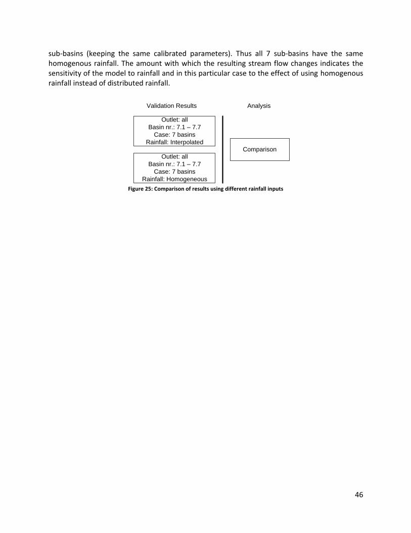
46

sub-basins (keeping the same calibrated parameters). Thus all 7 sub-basins have the same homogenous rainfall. The amount with which the resulting stream flow changes indicates the sensitivity of the model to rainfall and in this particular case to the effect of using homogenous rainfall instead of distributed rainfall.

Comparison

Outlet: all

Basin nr.: 7.1 – 7.7

Case: 7 basins

Rainfall: Interpolated

Outlet: all

Basin nr.: 7.1 – 7.7

Case: 7 basins

Rainfall: Homogeneous

Validation Results Analysis

Figure 25: Comparison of results using different rainfall inputs

47

5. Results

The methods that were discussed in the previous chapter have been applied and an overview of the resulting output is provided in this chapter. First the results of the rainfall and stream flow interpolation are shown in Section 5.1. This gives insight in the uncertainty of the rainfall and stream flow data. Then the results of the sensitivity analysis are provided in Section 5.2. Section 5.3 contains calibration and validation results for each basin delineation. In Section 5.4 the effects on model output of using multiple HRUs are shown and in Section 5.5 effects on model output of adjusting rainfall are shown. The results are discussed in Chapter 6.

5.1. Rainfall and stream flow interpolation

Both rainfall and stream flow data are interpolated according to the procedures described in the previous chapter. The results of the rainfall interpolation are summarized in Section 5.1.1. and the results of the stream flow interpolation in Section 5.1.2.

5.1.1. Rainfall Interpolation

First the data gaps in all 67 rain stations are interpolated. There were 6 stations that did not contain sufficient data to perform the interpolation, because they did not have at least one complete year of data. These stations (41, 42, 43, 44, 50 and 56) are excluded from any further analysis and are also not used when generating the rain stations used in SWAT. Cumulative mass curves of the remaining stations are plotted in Figure 26 to indicate any irregularities. As can be seen two stations do not comply with the general trend. These stations are nr. 36 and nr. 61 which are outside the basin area (see map Appendix E) and are located at an elevation of 2345 and 2344 m a.m.s.l. respectively. These elevations are average compared to the elevations of the other stations and so these very high rainfall levels cannot be explained. Together with the stations that did not have sufficient data they will be omitted when generating the rain stations used in SWAT. The other 59 stations appear to be consistent with the general trend, aside from some minor irregularities.

Figure 26: Cumulative mass curves of 67 rain stations

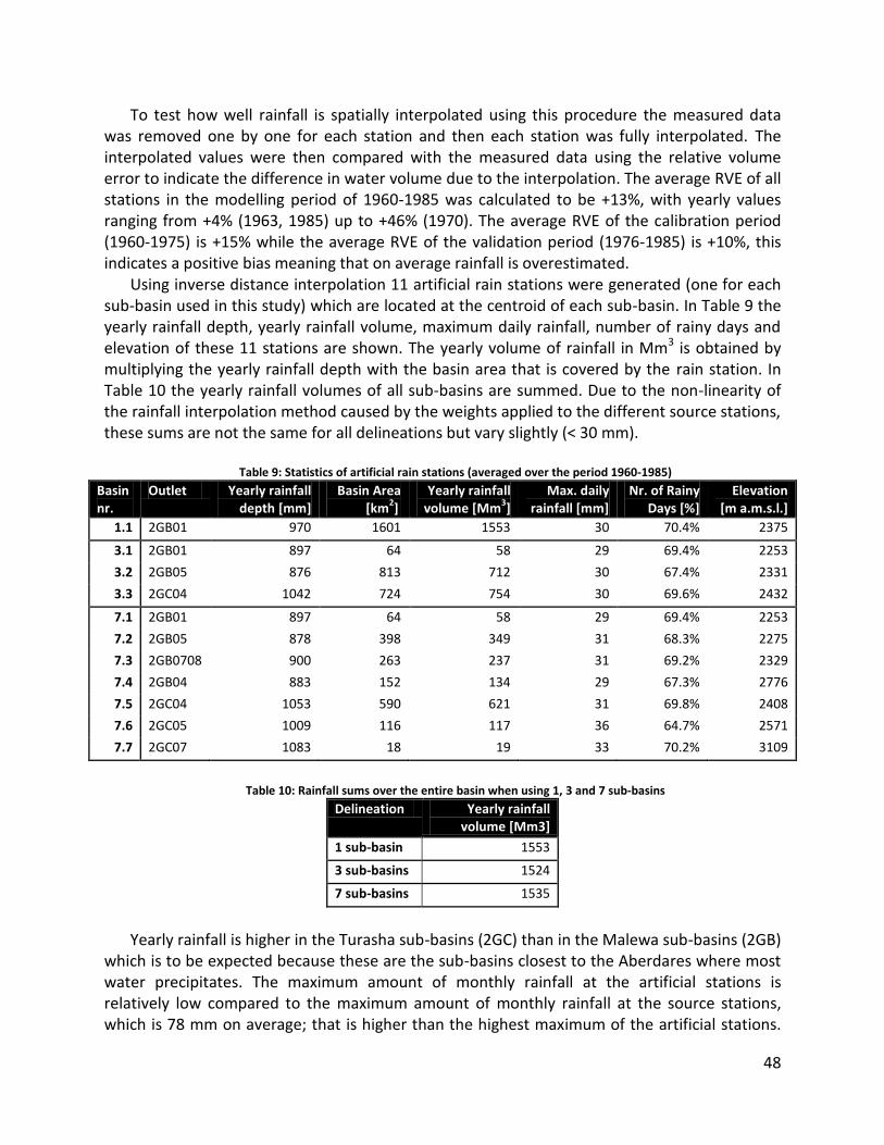
48

To test how well rainfall is spatially interpolated using this procedure the measured data was removed one by one for each station and then each station was fully interpolated. The interpolated values were then compared with the measured data using the relative volume error to indicate the difference in water volume due to the interpolation. The average RVE of all stations in the modelling period of 1960-1985 was calculated to be +13%, with yearly values ranging from +4% (1963, 1985) up to +46% (1970). The average RVE of the calibration period (1960-1975) is +15% while the average RVE of the validation period (1976-1985) is +10%, this indicates a positive bias meaning that on average rainfall is overestimated.

Using inverse distance interpolation 11 artificial rain stations were generated (one for each sub-basin used in this study) which are located at the centroid of each sub-basin. In Table 9 the yearly rainfall depth, yearly rainfall volume, maximum daily rainfall, number of rainy days and elevation of these 11 stations are shown. The yearly volume of rainfall in Mm3 is obtained by multiplying the yearly rainfall depth with the basin area that is covered by the rain station. In Table 10 the yearly rainfall volumes of all sub-basins are summed. Due to the non-linearity of the rainfall interpolation method caused by the weights applied to the different source stations, these sums are not the same for all delineations but vary slightly (< 30 mm).

Table 9: Statistics of artificial rain stations (averaged over the period 1960-1985)

Basin nr.

Outlet Yearly rainfall depth [mm]

Basin Area [km

2]

Yearly rainfall volume [Mm

3]

Max. daily rainfall [mm]

Nr. of Rainy Days [%]

Elevation [m a.m.s.l.]

1.1 2GB01 970 1601 1553 30 70.4% 2375

3.1 2GB01 897 64 58 29 69.4% 2253

3.2 2GB05 876 813 712 30 67.4% 2331

3.3 2GC04 1042 724 754 30 69.6% 2432

7.1 2GB01 897 64 58 29 69.4% 2253

7.2 2GB05 878 398 349 31 68.3% 2275

7.3 2GB0708 900 263 237 31 69.2% 2329

7.4 2GB04 883 152 134 29 67.3% 2776

7.5 2GC04 1053 590 621 31 69.8% 2408

7.6 2GC05 1009 116 117 36 64.7% 2571

7.7 2GC07 1083 18 19 33 70.2% 3109

Table 10: Rainfall sums over the entire basin when using 1, 3 and 7 sub-basins

Delineation Yearly rainfall volume [Mm3]

1 sub-basin 1553

3 sub-basins 1524

7 sub-basins 1535

Yearly rainfall is higher in the Turasha sub-basins (2GC) than in the Malewa sub-basins (2GB)

which is to be expected because these are the sub-basins closest to the Aberdares where most water precipitates. The maximum amount of monthly rainfall at the artificial stations is relatively low compared to the maximum amount of monthly rainfall at the source stations, which is 78 mm on average; that is higher than the highest maximum of the artificial stations.

49

This happens because high values for some of the source stations are levelled out by lower values of other stations as it is unlikely that there is a peak in rainfall for all stations at the same time. Because of this the peaks in rainfall are underestimated which means peaks in surface runoff are also reduced since most of this occurs during extreme rainfall events. However, this definition of ‘underestimation’ assumes that one specific station or ‘point’ is representative for the entire basin area that it covers and that the entire basin (or sub-basin) would receive the same amount of rainfall as measured on that specific point. In reality rainfall is much more variable especially considering the fact that (sub-)basins in this study may range up to 1600 km2, this means that an underestimation of rainfall especially during storm events may in fact be more compliant with the physical reality. This is supported by Sivapalan & Blöschl (1998) who state that for extreme rainfall events an adjustment coefficient should be applied to reduce rainfall measured at a point station in order to represent areal rainfall. In relation to this the number of rainy days has increased as compared to number of rainy days measured at the source stations, because now there are more days with little rainfall. This happens due to the effect of levelling out, because on almost every day it rains on at least one location in the basin, this rainfall will contribute to the interpolation resulting in a larger number of smaller values at the stations that are being interpolated. This ‘overestimation’ of rainy days can be explained as a positive contribution to modelling the physical reality because, especially in larger basins, rain can be very local and may not be caught by one of the rain stations.

So in short; peaks in rainfall are underestimated and the number of rainy days is overestimated where the net effect, in this case, is a positive bias of 13%. However, this is calculated based on rain stations located at specific points, when considering that these gauges represent entire basin areas these effects (reduction of peaks and increase in rainy days) are to be expected and may in fact be a better representation of areal rainfall.

Table 11: Statistics of interpolated river gauging stations (considered over the period of 1960-2010), stations marked

with an asterisk are used in SWAT

RGS RVE Max. flow [m3/s] Mean flow [m

3/s] No flow [%]

2GA03 0.3% 17.59 0.77 0

2GB01* 0.6% 90.79 5.87 0

2GB03 9.4% 7.29 0.53 0

2GB04* 2.0% 13.53 1.09 0

2GB05* -3.5% 116.86 3.32 0

2GB0708* -2.7% 144.35 2.19 0

2GC04* 0.6% 136.72 4.75 0

2GC05* -1.5% 9.66 0.87 0

2GC07* 1.4% 3.35 0.22 0

2GC10 0.4% 4.41 1.05 0

2GD02 -4.2% 80.15 0.56 36.9

2GD07 10.3% 67.06 0.42 60.3

50

5.1.2. Stream flow interpolation

Missing data in river gauging stations are interpolated according to the methods described in Chapter 4. Twelve stations have been interpolated of which seven are used in this study. The stations and their characteristics are shown in Table 11; stations marked with an asterisk are the ones that are used. The stations 2GA01, 2GA05 and 2GA06, mentioned in Chapter 4, are not interpolated as they are considered to be too unreliable. The stations 2GA03, 2GB03, 2GC10, 2GD02 and 2GD07 will not be used either as explained in Chapter 4 but they were interpolated nonetheless for future usage. 2GB01 was interpolated as well according to the method of Hughes & Smakhtin (1996) but is replaced by the sum of 2GB05 and 2GC04. This was done because the measured data contained a large number of inconsistencies which is proven by the fact that the mean of 2GB01 is much lower than the sum of the means of its two upstream tributaries (in Table 11 the characteristics of 2GB01 are shown before using the sum of 2GB05 and 2GC04). The RVE in Table 11 reflects the relative volume error caused by the interpolation method. The RVE is calculated by removing the measured data one by one for each station and then applying the interpolation method. The average RVE is +1.1% which is a good result especially compared to the interpolation of rainfall data. The 2GB03 and 2GD07 station have the worst performance with +9.4% and +10.3%. As expected no flow periods only occur for both RGS in the Karati River (2GD02 and 2GD07) as this river has intermittent stream flows. The other rivers are perennial; this is due to the continuous amounts of water stream flowd from the Aberdares.

5.2. Sensitivity analysis

Three different basin delineations are used, one coarse delineation with only one sub-basin, one case with three sub-basins and one case with 7 sub-basins. This results in 11 sub-basins in total as shown in Figure 22 (Chapter 4). For each sub-basin the sensitivity of 20 parameters is calculated and the parameters are ranked. The summarized results are shown in Figure 27 and Figure 28. A detailed overview of the values related to these graphs is provided in Appendix H. The sensitivity of model output to a change in a parameter was calculated based on two criteria; firstly on the percentage of change in mean stream flow at the outlet of each basin (Figure 27) and secondly on the percentage of change in the objective function (Figure 28).

When considering the percentage of change in mean flow it can be seen that changes in the maximum canopy storage (Canmx) and the maximum leaf area index (Blai) have a large impact. This is because together they determine the amount of rainfall that can be stored on the canopy cover which determines how much water reaches the surface and how much water is evaporated. Also the Curve Number for soil moisture condition II (CN2) plays an important role in some but not in all basins. CN2 is the parameter that determines the amount of water that infiltrates into the soil storage and the amount that will become surface runoff, the parameter has low sensitivity results for sub-basins 3.3 (2GC04), 7.4 (2GB04), 7.5 (2GC05) and 7.7 (2GC07). These basins have in common that they all have Forest Evergreen (FRSE) as their land use type which results in more water being retained by the canopy and less surface runoff to occur, which explains why a change in CN2 will have less impact.

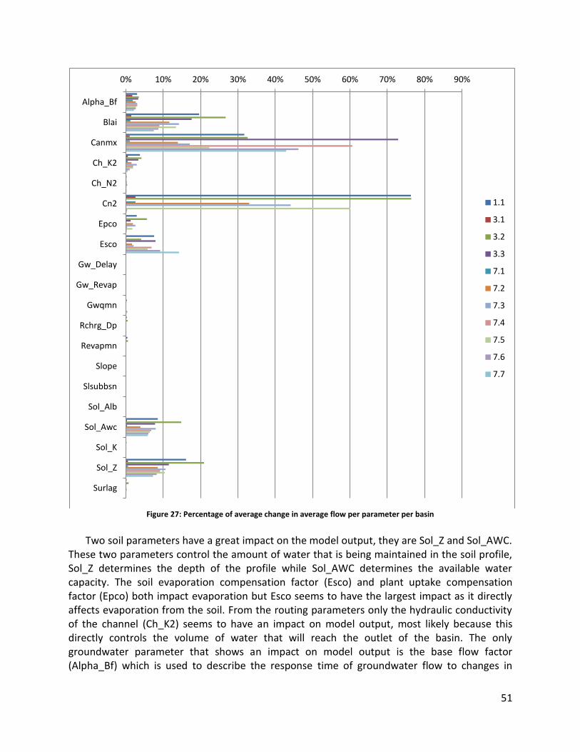
51

Figure 27: Percentage of average change in average flow per parameter per basin

Two soil parameters have a great impact on the model output, they are Sol_Z and Sol_AWC.

These two parameters control the amount of water that is being maintained in the soil profile, Sol_Z determines the depth of the profile while Sol_AWC determines the available water capacity. The soil evaporation compensation factor (Esco) and plant uptake compensation factor (Epco) both impact evaporation but Esco seems to have the largest impact as it directly affects evaporation from the soil. From the routing parameters only the hydraulic conductivity of the channel (Ch_K2) seems to have an impact on model output, most likely because this directly controls the volume of water that will reach the outlet of the basin. The only groundwater parameter that shows an impact on model output is the base flow factor (Alpha_Bf) which is used to describe the response time of groundwater flow to changes in

0% 10% 20% 30% 40% 50% 60% 70% 80% 90%

Alpha_Bf

Blai

Canmx

Ch_K2

Ch_N2

Cn2

Epco

Esco

Gw_Delay

Gw_Revap

Gwqmn

Rchrg_Dp

Revapmn

Slope

Slsubbsn

Sol_Alb

Sol_Awc

Sol_K

Sol_Z

Surlag

1.1

3.1

3.2

3.3

7.1

7.2

7.3

7.4

7.5

7.6

7.7

52

recharge. The impact of groundwater parameters is insignificant (<1%) in this analysis because the amount of water percolating from the soil storage into the shallow aquifer is relatively low as compared to the amount of water flowing to the reach directly from the soil storage as lateral flow. Other parameters such as Slope, Slsubbsn, Ch_N2 and Surlag seem to have little effect; this is most likely because results are assessed at a monthly scale while these parameters have more effect on smaller time scales.

Figure 28: Percentage of average change in objective function per parameter per basin

When considering the percentages of change in objective function as a criterion for

sensitivity (Figure 28) the results are more or less similar with one large exception which is that Alpha_Bf now plays a much more important role. Whereas the mean flow criterion only considers changes in total flow volume the objective function criterion also assesses the impact

0% 20% 40% 60% 80% 100% 120% 140% 160% 180% 200%

Alpha_Bf

Blai

Canmx

Ch_K2

Ch_N2

Cn2

Epco

Esco

Gw_Delay

Gw_Revap

Gwqmn

Rchrg_Dp

Revapmn

Slope

Slsubbsn

Sol_Alb

Sol_Awc

Sol_K

Sol_Z

Surlag

1.1

3.1

3.2

3.3

7.1

7.2

7.3

7.4

7.5

7.6

7.7

53

on the flow pattern, therefore a parameter that controls the timing of ground water flow such as Alpha_Bf can have a much larger impact. Also the surface runoff lag and Manning’s coefficient have a greater impact using this criterion because they both affect the stream flow pattern by delaying the flows when increasing the parameter value. However, the impact is not as significant on a monthly scale, because both parameters act on smaller time scale (days instead of months).

5.3. Basin delineation

Each sub-basin was calibrated using data from 1960 up to 1975 including a two year warm-up period and validated using data from 1974 up to 1985, including a two year warm-up period as well which overlaps with the last two years of the calibration period. The objective function used during the calibration aimed at minimising the mean squared error (MSE) as explained in Chapter 4. After the calibration the model was run with the calibrated parameters to simulate stream flows for the validation period. For each sub-basin the relative volume error (RVE) and the Nash-Sutcliffe efficiency (NSE) are calculated for both the calibration and validation period. The results are shown in Table 12. At every sub-basin parameter convergence occurred during calibration which means that a calibration session was never terminated prematurely and an optimum meeting the criteria was always found. The number of iterations required during a calibration run varied per sub-basin and ranged between 4000 and 8000. There is no correlation between the number of iterations and any basin characteristic or model result, indicating that the calibration method does not result in a bias of some sort.

Table 12: RVE and NSE of monthly stream flows for each sub-basin

Basin nr. Outlet RVE (Calibration)

NSE (Calibration)

RVE (Validation)

NSE (Validation)

1.1 2GB01 -1% 0.47 5% 0.71

3.1 2GB01 1% 0.56 6% 0.74

3.2 2GB05 -6% 0.44 8% 0.52

3.3 2GC04 -1% 0.37 -7% 0.51

7.1 2GB01 -8% 0.57 9% 0.76

7.2 2GB05 -5% 0.51 20% 0.56

7.3 2GB0708 -7% 0.43 5% 0.54

7.4 2GB04 -11% 0.46 7% 0.46

7.5 2GC04 -9% 0.35 2% 0.63

7.6 2GC05 -2% 0.38 6% 0.60

7.7 2GC07 -8% 0.52 -3% 0.76

To interpret these results in relation to the issue of scale the NSE is compared at similar

outlets within the three different basin delineations. The first and foremost outlet to compare is the most downstream outlet which is the same for all delineations, 2GB01. A comprehensive overview is shown in Figure 29. It shows that for both the calibration and validation periods the NSE increases with the number of sub-basins used in the delineation. Calibration results range from 0.47 up to 0.57 while validation results range between 0.71 and 0.76. For 2GB05 and

54

2GC04 only the cases with 3 and 7 sub-basins can be compared. 2GB05 follows the same trend as 2GB01 with better results at the finest delineation (Figure 30). 2GC04 shows the same trend for the validation period but an opposite trend for the calibration period as the NSE drops from 0.37 in the case with 3 sub-basins to 0.35 in the case with 7 sub-basins (Figure 31). Because only model validation is indicative for model performance it appears that applying a finer basin delineation results in better model performance.

Figure 29: Nash-Sutcliffe efficiency of simulated stream flows at the 2GB01 outlets for both the calibration and

validation periods

Figure 30: Nash-Sutcliffe efficiency of simulated stream flows at the 2GB05 outlets for both the calibration and

validation periods

Figure 31: Nash-Sutcliffe efficiency of simulated stream flows at the 2GC04 outlets for both the calibration and validation

periods

In all cases the NSE for the calibration period is considerably lower than that of the

validation period. Under ideal circumstances, where data are of the same quality during the entire period, the results of the calibration are expected to be either equal or better than those of the validation period. This suggests that the quality of the data used during the calibration period is much lower than that of the data used during the validation period. To test this, the case with 1 sub-basin was calibrated and validated again using the period of 1976 up to 1985 for calibration and 1962 up to 1975 for validation. The results are shown in Table 13. The resulting NSE of the new calibration period was 0.71, while the NSE of the validation period was now 0.39. In the old scenario the NSE of calibration was 0.47 while the NSE of validation was 0.71. So in both cases the NSE is much lower during the period of 1962 up to 1975 (0.39 and

55

0.47 as opposed to 0.71 and 0.71 for 1976-1985). These results suggest that data quality is indeed worse for the period of 1962 up to 1975.

Table 13: RVE and NSE of monthly stream flow simulation before and after reversing the calibration period

Basin nr. Outlet Calibration period

Validation period

RVE (Calibration)

NSE (Calibration)

RVE (Validation)

NSE (Validation)

1.1 2GB01 1962-1975 1976-1985 -0.01 0.47 0.05 0.71

1.1 2GB01 1976-1985 1962-1975 0.04 0.71 -0.13 0.39

Figure 32: Relative Volume Error of simulated stream flows at the 2GB01 outlets for both the calibration and validation

periods

Figure 33: Relative Volume Error of simulated stream flows at the 2GB05 outlets for both the calibration and validation

periods

Figure 34: Relative Volume Error of simulated stream flows at the 2GC04 outlets for both the calibration and validation

periods

Unlike the NSE, the RVE does not show a pattern where results become better when using

more sub-basins in the delineation. When considering the 2GB01 outlet an opposite trend can be observed, especially in the validation results (Figure 32) as the RVE seems to be closer to zero for coarser delineations, but this trend does not hold for calibration results of 2GB05 (Figure 33) and validation results of 2GC04 (Figure 34). In most cases the RVE is between ±10% except for validation of the 2GB05 sub-basin in the case with 7 sub-basins where it is +20%. An explanation for this high RVE could be that the observed mean flow at the 2GB05 outlet is 11% lower during the validation period as compared to the calibration period, while yearly rainfall

56

increases with 3% in this period. Because the MSE was used as a criterion for calibration the RVE is not necessarily minimised, since it is sensitive to the sign of the error implying that an underestimation in one month can compensate an overestimation in the next month. The average RVE during calibration is -5% while the average RVE during validation is +5% meaning that during validation the model tends to overestimate stream flows. By looking at the hydrographs these results can be interpreted in more detail.

The hydrographs of the validation period at the most downstream outlet (2GB01) are shown in Figure 35 (1 sub-basin), Figure 36 (3 sub-basins) and Figure 37 (7 sub-basins). In all three hydrographs it appears that peak flow recession is not modelled very well as the simulated peak flows tend to decline slower than observed peak flows, this may suggest that the base flow factor (Alpha_Bf) that regulates the timing and amount of base flow could still be improved. However, there are also peaks where the recession matches very well so adjusting the base flow factor would have negative effects for those peaks. Also, adjusting the base flow factor to create steeper peak flow recession may results in underestimation of base flows.

In Figure 38 the observed and simulated stream flow at the three 2GB01 outlets are plotted against each other. From the figure it can be derived that low flows tend to be overestimated while peaks are generally underestimated.

Figure 35: Hydrograph sub-basin 1.1, validation period 1976-1985

Figure 36: Hydrograph sub-basin 3.1, validation period 1976-1985

57

Figure 37: Hydrograph sub-basin 7.1, validation period 1976-1985

Figure 38: Observed versus simulated monthly averaged stream flows at the 2GB01 outlet

Yearly averaged water balance components for the calibration period using the calibrated

parameters are shown in Table 14. The calibrated parameter values themselves are shown in Table 15 and Table 16. The most notable results are the values of the three components that

58

contribute to the water yield (surface runoff, groundwater flow from the shallow aquifer and lateral flow from the soil storage). Surface runoff and groundwater flow are zero for a number of sub-basins. Lateral flow almost completely dominates water yield for sub-basins 1.1, 3.2, 3.3, 7.2 and 7.7. These sub-basins have in common that either their Sol_AWC or their Sol_K (or both) are relatively high which means that there is a lot of available water capacity in the soil storage and that the hydraulic conductivity is very high, resulting in large amounts of lateral flow. Surface runoff is zero or close to zero in all cases except for sub-basin 7.3 where it makes up the total water yield. This is directly related to the fact that Sol_K is zero for this sub-basin and thus no water flows through the soil while there is a large surplus of water available (subtracting ET from rainfall gives 162.5 mm) which means most of this water needs to be transported through surface runoff. For sub-basin 7.1 Sol_K is zero as well, but here the surplus of water is much smaller (21.7 mm) and is absorbed by the soil storage because the capacity of the soil storage (combination of Sol_Z and Sol_AWC) is much larger. The water then remains in the soil storage because Sol_K is zero and the water cannot be transported through the soil. Groundwater flow is very large in sub-basins 3.1 and 7.4 which both have in common that their Sol_K is very high while their Rchrg_Dp is zero. This means that large amounts of water are allowed to percolate from the soil storage to the shallow aquifer while no water is diverted to the deep aquifer. So there is much water allocated to the shallow aquifer which therefore results in large groundwater flows.

Apparently these values for these three flow components, when combined into water yield and added to the routing storage, result in stream flows that fit best with the observed stream flow data. Because there are no data available to calibrate each component individually nothing can be said about physical credibility of these values. It seems highly unlikely that there is so little surface runoff as multiple observations of large amounts of surface runoff during a wet period in May 2012 in sub-basin 7.5 (and therefore also sub-basin 1.1 and 3.3) were made. These observations were made 38 years after the modelling period, but the soil composition which is one of the important factors that determine if water infiltrates or becomes surface runoff will not have changed that much, so the observations are a good indication. Thus, the SWAT model is able to simulate stream flows quite well when looking only at the stream flow outlet, but when looking at the internal flow values of the model they appear to be unrealistic.

Sub-basin 3.1 and 7.1 were expected to be hydrologically inactive (Chapter 4) as observed inflows equal observed outflow (2GB05+2GC04=2GB01). However, after calibration only sub-basin 7.1 does not produce any water yield. The reason that sub-basin 3.1 does have a water yield may be because there is a negative RVE at the outlets of the two upstream sub-basins 2GB05 and 2GC04 which means inflow is underestimated and hence the model tries to compensate for this (during calibration) by adding more water to the routing storage and thus increasing the outgoing stream flow. However, the same applies to sub-basin 7.1, but this sub-basin has a much higher NSE for 2GB05 (and only slightly lower for 2GC04) which means that during calibration sub-basin 7.1 does not need to compensate as much.

PET values differ per sub-basin. For sub-basins 7.4, 7.6 and 7.7 PET values are considerably lower than for the other sub-basins. This is related to the weather station that is used in a sub-basin; the sub-basins with low PET values use weather statistics from the weather station located high up in the Aberdares to generate solar radiation and temperatures. The other sub-

59

basins use the weather station that represents the Kinangop Plateau which is much drier (less clouded) and located at a lower elevation, resulting in higher PET values.

Table 14: Detailed yearly averaged SWAT model output per sub-basin for the calibration period (1962-1975)

Basin nr.

Outlet Rainfall [mm] PET [mm] ET [mm]

Surface Runoff [mm]

Groundwater Flow [mm]

Lateral Flow [mm]

Water Yield [mm]

1.1 2GB01 940 1483 815 0 0 134 134

3.1 2GB01 869 1492 565 5 154 2 162

3.2 2GB05 863 1502 752 0 0 133 133

3.3 2GC04 998 1481 873 0 0 137 137

7.1 2GB01 869 1492 848 0 0 0 0

7.2 2GB05 863 1498 769 0 0 109 109

7.3 2GB0708 887 1490 724 140 0 0 140

7.4 2GB04 860 932 683 2 121 64 188

7.5 2GC04 1011 1480 891 1 40 64 104

7.6 2GC05 952 940 709 1 53 152 206

7.7 2GC07 1037 916 704 1 0 346 347

Table 15: Optimal parameter values for the 1 and 3 sub-basin delineations

Parameters Unity Basin 1.1 Basin 3.1 Basin 3.2 Basin 3.3

Alpha_Bf - 0.57 0.26 0.41 0.17

Canmx mm 9.16 8.41 9.96 0.29

Ch_K2 mm/hr 52.85 38.00 136.37 110.36

Ch_N2 - 0.12 0.27 0.05 0.16

CN2 - 65.60 66.38 82.94 62.43

Epco - 0.26 0.41 1.00 0.21

Esco - 0.66 0.95 0.96 0.89

GW_Delay days 174.21 196.36 430.58 401.72

GW_Revap - 0.13 0.10 0.03 0.10

GWqmn mm 273.58 353.92 194.25 1497.00

HRU_SLP (slope) m/m 0.49 0.00 0.52 0.59

Rchrg_dp - 0.58 0.00 0.19 0.92

Revapmn mm 273.79 258.69 122.01 398.84

Slsubbsn m 126.45 73.98 136.10 135.50

Sol_Alb - 0.10 0.00 0.06 0.21

Sol_AWC - 0.26 0.00 0.38 0.23

Sol_K mm/hr 36.47 772.37 112.87 26.19

Sol_Z(1) mm 160.17 166.27 189.87 60.63

Sol_Z(2) mm 1377.43 1247.00 2088.57 521.38

Sol_Z(3) mm 3500.00 3325.32 3500.00 1327.71

60

When looking at the individual parameters (Table 15 and Table 16) some remarks can be made. Values for Canmx (range: 0 - 10 mm) are either very high (> 8 mm) or very low (< 1 mm) for all sub-basins except for 7.5 which has an intermediate value of 5.6. This difference between Canmx values is caused by the land use type that is used (Table 17). Low Canmx values relate to a forest type land use while high Canmx values relate to brush and grasslands. A reason for this is that forest land use types have larger canopies and hence require less canopy storage depth to produce the same amount of evaporation. Sol_Alb is zero for sub-basin 3.1 and 7.1 which means that solar radiation is not absorbed and everything is reflected and therefore PET will obtain its maximum value given the weather station that is used. GWqmn is zero for sub-basin 7.5 and very low for sub-basin 7.6, this explains why there is also groundwater flow and not only lateral flow in those sub-basins because GWqmn is the threshold for groundwater flow to occur. CN2 is 83 for sub-basin 3.2, but only between 62 and 66 for sub-basins 7.2, 7.3 and 7.4 which together represent the same basin area as sub-basin 3.2. This indicates that at a finer scale processes are schematised differently, as the results in Table 14 also show, because for sub-basin 3.2 there is only lateral flow, while for sub-basins 7.3 and 7.4 there is also surface runoff and lateral flow.

Table 16: Optimal parameter values for the 7 sub-basin delineation

Parameters Unity Basin 7.1 Basin 7.2 Basin 7.3 Basin 7.4 Basin 7.5 Basin 7.6 Basin 7.7

Alpha_Bf - 0.32 0.39 0.11 0.07 0.66 0.75 0.18

Canmx mm 10.00 10.00 8.56 0.29 5.58 0.07 0.11

Ch_K2 mm/hr 2.68 21.85 68.16 26.94 79.85 72.49 108.06

Ch_N2 - 0.28 0.21 0.12 0.03 0.24 0.17 0.05

CN2 - 68.39 62.14 66.33 64.13 61.70 62.91 70.44

Epco - 0.78 0.16 1.00 1.00 0.55 0.33 0.52

Esco - 0.95 0.59 0.89 0.75 0.51 0.61 0.04

GW_Delay days 0.00 37.88 500.00 119.92 112.19 337.33 421.80

GW_Revap - 0.20 0.19 0.20 0.06 0.11 0.10 0.11

GWqmn mm 589.60 1246.80 1421.30 170.58 0.00 81.02 1644.60

HRU_SLP (slope) m/m 0.07 0.21 0.25 0.09 0.20 0.23 0.56

Rchrg_dp - 0.35 0.54 0.86 0.00 0.37 0.46 0.51

Revapmn mm 0.00 274.97 350.92 330.95 296.48 375.56 406.55

Slsubbsn m 150.00 104.84 150.00 138.44 115.92 127.96 121.39

Sol_Alb - 0.00 0.14 0.08 0.08 0.25 0.20 0.17

Sol_AWC - 0.38 0.43 0.03 0.05 0.24 0.34 0.86

Sol_K mm/hr 0.00 190.44 0.00 316.74 33.77 49.65 176.34

Sol_Z(1) mm 129.45 190.00 164.54 136.37 64.01 24.00 58.16

Sol_Z(2) mm 970.85 1425.00 1809.97 1377.31 550.49 206.40 587.37

Sol_Z(3) mm 2588.92 3500.00 3500.00 2795.52 1401.82 525.60 1192.18

61

Table 17: HRU definition of the basin delineations with 1, 3 and 7 sub-basins using one HRU per sub-basin

Basin nr. Outlet Land Use Soil Type Slope Class Basin area [%]

1.1 2GB01 Range-Grasses L21 0 - 80% 100.00%

3.1 2GB01 Range-Brush H9 0 - 80% 4.01%

3.2 2GB05 Range-Brush L22 0 - 80% 50.77%

3.3 2GC04 Forest-Evergreen L21 0 - 80% 45.21%

7.1 2GB01 Range-Brush H9 0 - 80% 4.01%

7.2 2GB05 Range-Brush H9 0 - 80% 24.84%

7.3 2GB0708 Range-Brush L22 0 - 80% 16.45%

7.4 2GB04 Forest-Evergreen M2 0 - 80% 9.49%

7.5 2GC04 Range-Grasses L21 0 - 80% 36.84%

7.6 2GC05 Forest-Evergreen L21 0 - 80% 7.24%

7.7 2GC07 Forest-Evergreen M2 0 - 80% 1.12%

5.4. HRU definition

Just like basin delineation the number of hydrological response units (HRUs) is also an issue of scale in hydrological model implementation. To test the effect of using different HRUs, four cases were studied using the delineation with only one sub-basin. The number of HRUs was increased as is shown in Table 18. Definition of HRUs works by selecting land use covering an area above a certain threshold first. Then only these land uses are used and are redistributed so that they cover the entire basin area. Within each land use the same is done with soils where soils covering areas above a certain threshold within a specific land use are selected and redistributed so together they cover the entire area of that specific land use. As a final step the same is done with slope classes within specific combinations of land use and soil type. In this case thresholds were chosen in such a way that only one soil type and slope class were defined per land use and thus land use was the factor that determined the number of HRUs. This was done because the important soil parameters that impact stream flows (Sol_Alb, Sol_AWC, Sol_K and Sol_Z) are used during calibration which makes the initial soil data input less relevant than the land use data which contains more parameters that are not being calibrated.

Table 18: Hydrological response units that were generated

HRU number

Land Use Soil type Slope Class

Original land use coverage

SWAT land use coverage

1 HRU 1 Range-Grasses L21 0 - 80% 27.50% 100.00%

2 HRUs 1 Range-Grasses L21 0 - 80% 27.50% 52.61%

2 Range-Brush L22 0 - 80% 24.77% 47.39%

3 HRUs 1 Range-Grasses L21 0 - 80% 27.50% 35.97%

2 Range-Brush L22 0 - 80% 24.77% 32.40%

3 Forest-Evergreen M2 0 - 80% 24.19% 31.64%

4 HRUs 1 Range-Grasses L21 0 - 80% 27.50% 31.78%

2 Range-Brush L22 0 - 80% 24.77% 28.63%

3 Forest-Evergreen M2 0 - 80% 24.19% 27.96%

4 Forest-Mixed H9 0 - 80% 10.06% 11.63%

62

In Table 17 the dominant land use class, soil type and slope class per sub-basin are shown. Only three dominant land use classes are defined which are range-grasses, range-brush and forest-evergreen. The soil types that occur are L21, L22, H9 and M2. In Table 18 the land use class, soil type and slope class are shown per HRU (using 1 sub-basin), in the case with 4 HRUs forest-mixed is defined which did not occur when using multiple sub-basins. The soil types for all 4 HRU definitions also occur when using multiple sub-basins with 1 HRU per sub-basin. In Figure 39 cumulative basin coverage of each land use type is shown when sorting land use based on their basin coverage. This shows that when using the 4 largest land use types about 85% of the basin area is covered. The SWAT land use coverage (and thus HRU) approaches the original land use coverage as model scale becomes finer and more land use types (HRUs) are added (Table 18). Therefore land use is more accurately represented at finer scales and thus better model results are expected with increasing HRUs.

Figure 39: Cumulative percentage of basin coverage with increasing land use type, where land use types have been sorted

ascending based on the size of the area that they cover

The results when using 1 up to 4 HRUs are visualised in Figure 40 and Figure 41. When

looking solely at validation results for the NSE it appears that the case with 1 HRU has the best performance. The case with 2 HRUs has the worst performance, but from there on the NSE gradually increases when the number of HRUs increases. This effect correlates with usage of range-brush which has most basin coverage when using 2 HRUs and then its coverage gradually declines. This suggests that range-brush does not represent the specific land use as it occurs in this tropical basin very well. However, when delineation the basin in sub-basins with 1 HRU per sub-basin, the sub-basins covered with range-brush do not perform worse than other sub-basins (Table 12 and Table 17). In appendix I the calibrated parameter values per HRU are shown. Other than the relation between Canmx and forest land use types mentioned before, there is no clear relation between calibrated parameter values and land use or soil types. This means that initial parameter values of parameters that are being calibrated (specifically those derived from the soil data) do not affect calibration results and any relation of these parameters with the original soil or land use data is lost during calibration.

63

When looking at the RVE no pattern can be observed, which indicates that increasing the number of HRUs does not necessarily improve model performance.

Figure 40: Nash-Sutcliffe Efficiency for multiple HRU

definitions

Figure 41: Relative Volume Error for multiple HRU definitions

5.5. Rainfall Adjustment

To assess what the impact of adjusting rainfall on model output is, a case was run for the delineation with 7 sub-basins where the same rainfall was used for each sub-basin. In this case the rainfall of sub-basin 1.1 was adjusted to fit to the sum of the rainfall used for sub-basin 7.1 to 7.7 (this sum differed slightly between each delineation as was shown previously in Table 10). This adjusted rainfall was applied to all sub-basins without re-calibrating any of them. Figure 42 shows the absolute change in monthly averaged stream flow (in m3/s) for the validation period (1976-1985). In Table 19 the changes in rainfall and changes in average stream flow are shown as percentages.

By using homogenous rainfall the relatively wet Turasha sub-basins (2GC) receive less rainfall while the relatively dry Malewa sub-basins (2GB) receive more rainfall. When rainfall increases stream flow increases as well and similarly when rainfall decreases stream flow decreases which is as expected. However, the change in stream flow is more than twice as large then the change in rainfall for all sub-basins except 7.1 and 7.7. For sub-basin 7.1 the change in stream flow is less than the change in rainfall. This happens because, as stated in Section 5.3, no flow is produced in this sub-basin, even when rainfall increases. This means that the stream flow out of sub-basin 7.1 is produced by upstream inflows and therefore does not relate to the change in rainfall in sub-basin 7.1. Thus, the change in outgoing stream flow is merely the net result of the changes in the stream flows of sub-basin 7.2 and 7.5 combined with some changes in transmission losses due to different flow volumes. These results show that adjusting rainfall has an amplified effect on stream flows and that therefore an accurate representation of rainfall at each scale is essential for modelling stream flows. They also show that the distribution of rainfall has an effect on the total volume of water that flows out of the basin because even though the total rainfall sum remains the same the amount of water that flows out of the basin increases. This can be attributed to the fact that the relation between rainfall and runoff is non-linear and differs per sub-basin. For example, when rainfall in one sub-basin increases with 10%, stream flow may increase with 20%, while when rainfall decreases with 10%, stream flows may decrease with only 15%.

64

Figure 42: Change in average daily stream flow when adjusting rainfall, calculated over the validation period (1976-1985)

Table 19: Effects of changes in rainfall on simulated mean flows over the validation period (1976-1985)

Basin nr. Outlet Interpolated Rainfall [mm]

Homogenous Rainfall [mm]

Change in Rainfall [%]

Change in mean flow [%]

7.1 2GB01 934 1018 9.02% 6.28%

7.2 2GB05 885 1018 15.08% 37.03%

7.3 2GB0708 899 1018 13.23% 38.99%

7.4 2GB04 905 1018 12.58% 32.00%

7.5 2GC04 1113 1018 -8.50% -26.27%

7.6 2GC05 1079 1018 -5.65% -13.73%

7.7 2GC07 1123 1018 -9.29% -14.09%

65

6. Discussion

This research focuses on scale issues in hydrological modelling. By using the Soil Water Assessment Tool (SWAT) the effects of scales of model implementation on stream flow were assessed and the results are shown in Chapter 5. In this chapter these results are discussed and compared with other results found in literature. In Section 6.1 issues related to data and model parameters are discussed, in Section 6.2 the calibration and validation methods are discussed. In Section 6.3 the results at the different scales are discussed and in Section 6.4 usage and limitations of the model in relation to water management are discussed.

6.1. Data and model parameters

Due to time restrictions no complete uncertainty analysis was performed. The accuracy of the interpolation methods for rainfall and stream flows was assessed. Nonetheless some qualitative remarks can be made with regard to uncertainties in data and model parameters and their impact on the results. The rainfall data used were obtained from the Kenyan Meteorological Department (KMD). This database contained a number of gaps which were filled using interpolation. However, a relatively large number of these gaps occurred in January which is the driest month. It may be possible that rather than being a gap it might have been a dry period without any rain in which no data was entered. This would cause an overestimation of rainfall as a relatively large number of potentially dry days need to be interpolated while there are less dry days with data available to use for interpolation. This could explain why in some periods of low (observed) stream flows there are relatively high values in rainfall. Also the effect of levelling out due to interpolation as explained in Section 5.1.1 causes the number of rainy days to increase, in SWAT this will have an effect on the generation of PET as this is partially calculated based on cloud cover which is connected to the number of rainy days. When the number of rainy days increase PET will decrease, in combination with an overestimation of rainfall this means that more water is available for surface runoff or infiltration in the model than there would be in reality. In SWAT this can be compensated by either increasing canopy storage (controlled by Canmx) or soil water storage (controlled by Sol_Z). This explains why Canmx and Sol_Z tend to become very high for especially the dry Malewa (2GB) sub-basins. In the wetter Turasha (2GC) sub-basins values for Canmx and Sol_Z are much lower, indicating that in these sub-basins overestimation of rainfall is not so much an issue because there are less dry days.

As was mentioned in the description of the methods, solar radiation and temperature series were generated using the algorithm available in ArcSWAT as there were no continuous data series available, just short periods of a few years. This algorithm uses monthly statistics derived from the few years that were available to generate the time series. However, the data used were more recent (1995-2012) than the modelling period (1960-1985). Also Arnold et al. (2011) suggest using at least 20 years of data so large uncertainties are introduced in the calculation of solar radiation and temperature and thus PET. Furthermore these variables were measured at only three stations which reduces the impact of using different basin delineations, especially since only two of these three stations were actually located within the study area (one was close to Lake Naivasha, but not within the Malewa basin). By estimating solar radiation and temperatures it is assumed that solar radiation and temperatures do not change significantly on

66

a monthly averaged basis within a period of 60 years, neglecting any effects of climate change. This may be true to some extent but the problem remains that each month has a different average temperature and solar radiation each year (f.e. January 1970 may be much warmer and sunnier than January 1971). Since this variability is modelled using a random generator, simulated values may be very different from actual values even though the long term statistics will match. This issue with solar radiation and temperatures which drive the calculation of PET is one of the largest uncertainties in the model. A possible way to improve this is to put measured PET values directly in the model. A daily series of pan evaporation values measured close to Lake Naivasha is available and could be scaled to represent PET at higher elevations using monthly PET values determined by Kalders (1988).

Of the 15 river gauging stations for which data was availably only 7 were actually used in this research as a number of them was not located in the Malewa (2GA, 2GD) basin or did not have data for the modelling period (2GB03, 2GC10). Also the data of 2GB01 was deemed to be unreliable and thus this station was replaced by the sum of its two nearby upstream tributaries 2GB05 and 2GC04. Since stream flow data are used for calibration it is important that these data are reliable. Despite the interpolation method being quite reliable (less than 5% RVE at all stations used) there still is a large uncertainty in the collection of the data. Firstly the readers that read the gauging staffs sometimes do not read water levels correctly or do not read them at all, especially when flows are high because either the gauging staffs are completely submerged, washed away or inaccessible. This implies that some peaks in stream flow have not been recorded resulting in an underestimation of stream flow. Secondly conversion of water levels to stream flows was done for the entire period of 1960-2010 using only one rating curve per station. The data points on which these rating curves are based have been obtained mostly during dry periods for practical reasons; this means that the high flow periods are not well covered. Also the curvature of the river bed may change over time (Figure 43) causing the relation between water level and stream flow to change. However, for the stations used in this study the river bed seems to have been relatively stable based on the fact that rivers and their gauging stations are still at the same location.

Figure 43: Changes in the shape of Little Gilgil at the 2GA06 RGS, next to the Malewa basin

67

The soil classification used was based on a map developed by the Kenyan Soil Survey in 1982. The resolution of the map was very coarse considering the high variability of the soils in the basin but SWAT also aggregates soils into dominant soil classes within HRUs and thus this coarse resolution fits the spatial scale of model structure. The properties of the soils in the soil map had to be converted to SWAT parameters. This conversion was based on a dataset with SWAT soil parameters assembled by Tiruneh (2003), but this data set was based on only a few measurements which did not cover the entire basin, therefore the most important soil parameters related to simulation of stream flows were calibrated. The calibrated soil parameters (Sol_AWC, Sol_Alb, Sol_K and Sol_Z) differ from the soil parameters in the data set in some cases by more than 100% which means that either the soil data set used was very poor or the calibration method was not able to generate the real parameters. The truth is most likely a combination of poor data and a model calibration method that is not aimed at simulating soil water in detail, only stream flows.

The land use map used had a much higher resolution than the soil map but not as many different classes. A problem that occurred was that there was no database with SWAT land use parameters for Kenya. This meant that the default SWAT parameters, typically set up for US land use classes, had to be used and connected to the land use map. Some of the parameters related to land use were therefore used during calibration such as CN2. But some other parameters could not be used such as the maximum leaf area index (Blai). The type of LULC and the parameters related to it have a significant impact on model outcomes. This was proven when changing, for example, ‘Range Bushes (RNGB)’ to ‘Agricultural land (AGRL)’. After re-calibration the NSE reduced with more than 0.2 at some of the outlets. This indicates poorer model results are to be expected for sub-basins with equally large but very different land use when using only one HRU per sub-basin. However, this is opposed by the fact that there is no significant improvement in stream flow simulation when increasing the number of HRUs as was shown in Figure 40. An explanation could be that specifically the change from RNGB to AGRL has a large impact because AGRL also affects some land management characteristics (the harvesting index for example), but this was not tested extensively in this research. There was no data on irrigation during the modelling period so the irrigation component of the model was turned off. Since there was only some small scale farming in the modelling period this assumption will only cause a minor error which is accounted for via calibration of the model parameters.

6.2. Sensitivity analysis and calibration

For each sub-basin a sensitivity analysis was performed to indicate the influence of each parameter on model output. Initially the analysis was run using only 10 Latin Hypercube (LH) loops which implied only 10 different parameter combinations. However, this number was very low considering the fact that 20 parameters were used; therefore another analysis was done using 100 LH loops. This still leaves a large part of the parameter space unexplored but nonetheless gives an indication of the relative sensitivity of model output to different parameters. The sensitivity analysis is not used directly to steer calibration because all parameters used in the analysis could also be used for calibration directly so it was not needed to select only the most sensitive ones. However, this may have caused effects of over-parameterization as is discussed later on in this chapter. The sensitivity analysis can still be used

68

to indicate which parameters should be considered specifically when analysing the results as they have the largest impact.

The Parasol calibration method in SWAT CUP was able to handle large numbers of parameters which means that all important stream flow related parameters that could be varied on a sub-basin scale could be calibrated in one calibration run. This accounts for most of the parameter interdependency and should result in finding a global optimum. Model performance may be improved by performing a second calibration run using smaller parameter ranges based on the results of the first run, but this is not likely to result in a significant improvement because parameters will not change with more than 0.5% of their range due to the 1% convergence criterion. Besides Parasol, SWAT CUP also provides a number of other calibration methods such as SUFI-2, MCMC and GLUE. Due to time limitations these were not tested for this case. Setegn et al. (2008) and Yang et al. (2008) did test these methods on basins in Ethiopia and China respectively. Their results indicate that Parasol produces the highest NSE values and is most suited when calibrating based on stream flow data using MSE as an objective function. Manual calibration is not an option in this type of comparative study because it would introduce a random component and potential bias rendering the results useless for comparison.

Observed stream flow data were used to drive calibration. As explained, these data were in fact interpolated as well using the methods developed by Hughes & Smakthin (1996). This interpolation method is relatively accurate but still introduces an additional error, but given the fact that there are no complete data series for this area this is the most optimal solution to use. No relation between the percentage of gaps that were interpolated and the model results (NSE values) at the different outlets is found, which means that the method does not introduce a bias of some sort.

Calibration was performed on a monthly time scale while the model runs on a daily time scale. Ideally calibration is also performed on a daily time scale but the data (especially rainfall data) were not deemed accurate enough as explained in Chapter 4. Because of this, some parameters that act on a sub-monthly time scale may not be calibrated properly. For example Manning’s roughness coefficient (Ch_N2) affects the speed of stream flow which does not have much effect on a monthly scale. This reduces the correctness of the physical representation of some parts of the model. Spatial scale also affects this correctness of physical representation, when larger sub-basins are used the processes become more aggregated but model structure does not change. This means that even if a good MSE is found for stream flows at the outlet of a sub-basin, the internal model results such as the division of flow between surface runoff, lateral flow and groundwater flow, may not have a physical representation anymore. The calibration objective function is not able to reward good simulation results of internal flows with low MSE values, because only the stream flow at the outlet is tested. The model becomes a sort of black box of which only the input and output hold any meaning.

Some of the parameters such as Canmx and Sol_Z are often calibrated close or at the upper boundaries of their range. This means better stream flow simulation results may have been obtained by extending the parameter range. However, Arnold et al. (2011) found, based on numerous study cases, that the given parameter ranges are the limits of feasible values that parameters can take and since there is no information available that indicates otherwise these ranges were kept.

69

An interesting characteristic of the results is that the NSE obtained for the calibration period is considerably lower than the one for the validation period at all sub-basins. Gassman et al. (2007) found that this is not uncommon and that in a number of other studies the same happened. This indicates that the quality of data used during the calibration period is much poorer as was tested in Chapter 5. When swapping calibration and validation period results remain poor for the period 1962-1975. From this it can be concluded that data quality is indeed worse for the period of 1962 up to 1975 as it appears that for this period the relation between rainfall and stream flow cannot be modelled very well, this underlines the importance of good quality of the data. Though this could also imply that SWAT is not suitable for modelling this basin, but considering the much better performances during the period of 1976 up to 1985 it seems more likely that the issue is data related. However, internal model results (surface runoff, lateral flow etc.) remain unrealistic for both cases.

Two other points of discussion are the usage of the MSE as objective function during calibration and the NSE as assessment criterion for both calibration and validation. The MSE does not consider the volume error that occurs over time. It aims at reducing each individual error but does not consider the sign of the error (positive or negative) which, for example, can result in a number of small negative errors that together may result in a larger negative volume error despite having a fairly good NSE. A multi-objective function using the RVE as a criterion as well might provide a better simulation of total stream flow volumes. Also the NSE (which is fact a normalization of the MSE) was used as main criterion for judging all model results. However, the NSE tends to be very sensitive to outliers (McCuen et al., 2006) implying that sub-basins with a small number of high peak flows tend to have a better NSE than basins with more lower peak flows. But this effect is not expected to play a role in the current study, because results are compared at stations with similar observed outflow and hence similar peak flows. Since simulated flows are calibrated on these observed flows they tend to have similar peak flows as well and hence the relative effect of this phenomenon on the NSE between similar outlets should not be significant. Legates & McCabe (1999) suggest combining the NSE with the coefficient of efficiency or the index of agreement, but for this study using the NSE is found to be sufficient to indicate effects of using different scales of model implementation as this is the most used statistic for stream flows simulations and is therefore easily comparable with other studies (Gassman et al., 2007).

6.3. Scale issues of model implementation

Three different basin delineations were applied, the results at the 2GB01 outlets of each delineation were compared as well as the results at the 2GB05 and 2GC04 outlets in the cases with 3 and 7 sub-basins. The results indicate that stream flow is less accurately simulated when using less sub-basins for basin delineation. This implies that aggregating spatial data into a coarser scale introduces a modelling error that cannot be compensated for by adjusting parameters during calibration.

To explain why finer basin delineations perform better than coarser basin delineation the actual model components in SWAT that are affected by delineation should be identified. Firstly the land use and soil parameters are modelled in more detail when using more sub-basins because in this study one HRU is defined per sub-basin for every delineation and also calibrated at this level. Secondly rainfall is distributed and specified for each sub-basin, just as other

70

weather data such as solar radiation and temperatures which affect PET, though it must be noted that only two weather stations acted as a source for calculation of all temperature and solar radiation series. Finally stream flow channel characteristics (such as bed roughness and hydraulic conductivity of the bed) are also modelled and calibrated in more detail when using a finer scale. Of these components especially rainfall distribution seems to have a large impact on stream flow simulation as was tested in Chapter 5 by applying homogeneous rainfall to the delineation with 7 sub-basins. To identify the impact of soils and land use, the impact of HRU definition, which is composed of soil types and land use classes (and slope classes), is studied as well.

To test if using multiple HRUs per basin would provide better results as is suggested by, for example, Setegn et al. (2008), the number of HRUs was increased for the case with one sub-basin. The simulation of stream flow did not improve and even became worse when using multiple HRUs. This is opposed as to what is expected but complies with Gassman et al. (2007), who found that only a few SWAT studies observed improvement of model performance when increasing the number of HRUs. One reason for this may be the effect of over-fitting of parameters. Because with each increase in HRUs a large number of parameters is added, the calibration approach may not be able to find the actual optimal solution as there are many sub-optimal solutions using completely different parameter combinations. These sub-optimal solutions can generate values of objective functions very close to the actual optimum so that the parameter convergence threshold may be reached for sub-optimal values. A second reason may be the fact that default SWAT values are used for all land use parameters instead of values that are specifically adjusted to this particular basin. Among these parameters is for example the maximum leaf area index (Blai) which, as shown before, is one of the most sensitive model parameters. Because these parameters have been developed for basins in the USA, they may not be translated one to one to the Malewa basin, introducing additional errors when using more HRUs.

A common solution to this problem of over-parameterization is to use a scaling factor to calibrate the model parameters (Abbaspour, 2011). For example, the Canmx parameter values for all HRUs can be calibrated by scaling them using only one parameter, the scaling factor. However, this approach assumes that the initial parameter values are known. By default Canmx is set to its default value, which is the same for every HRU regardless of the land use that is used. This means that for this particular parameter it does not matter if there are multiple HRUs or only one. Other parameters such as the soil parameters do have specific values that differ per HRU but when they are scaled it is assumed that the relative difference between these parameter values is correct. Considering the uncertainty in the soil data this may introduce a large error. Using a scaling factor is therefore not a good approach and so the problem with over-parameterization when using multiple HRUs per basin remains. Therefore the amount of HRUs in this study could only be increased to 4 because with 5 or higher the ParaSol calibration scheme could not handle the number of parameters anymore.

Another solution to over-parameterization is to collect more data to estimate the parameters. By estimating the parameters based on actual data, they do not have to be calibrated, reducing the number of parameters used during calibration. This solution in fact relates to the issue of scales of observations versus scales of model implementation as mentioned in Chapter 1. Because SWAT is a very complex model, the current data availability

71

may not have been sufficient to use the model it its full extent. Since there was no data on internal flows such as surface runoff, lateral flows and internal flows they could not be calibrated. If this data would be available better internal model results would be achieved.

A final remark with regard to the effects of using finer basin delineations is that uncertainty in data is very large and that the differences in stream flow simulations (quantified using the NSE) are not so large. In Section 5.1 is stated (and quantified) that uncertainty in rainfall data is large even when only considering the uncertainty in the interpolation method used. In addition to that it was found in Section 5.5 that SWAT, as expected, is very sensitive to rainfall input. Adding to that the uncertainty in variables such as solar radiation and temperatures indicates that outcomes are very uncertain. It is therefore uncertain if from the resulting NSE values it can actually be concluded that a finer scale of model implementation indeed results in a better simulation of stream flows. After all, the noise in the results caused by uncertainty should not be larger than the effects caused by using different spatial scales as stated by Merz et al. (2009) (Chapter 1). However, if this uncertainty would indeed be larger than the trend of better results at finer basin delineations, then the trend may not be observed or only for a few cases, while in this study the trend was observed for all sub-basins. It is therefore safe to say that stream flow simulation results do improve when increasing the number of sub-basins.

6.4. Water management

Initially one of the basin delineations to be studied was a delineation that followed the management boundaries of the Water Resources Users Associations (WRUAs). This delineation could then be used to see if the current water management boundaries are the most optimal. It could also be used to study impacts of land use change on stream flow. However, a problem that occurred was that locations of the river gauging stations did not match the boundaries of WRUAs, hence it would be impossible to calibrate and validate the sub-basins properly. An option would be to use downstream stations but then it is not possible to study actual effects of changes within a specific WRUA because they may be merged with other effects downstream. Another issue that came up with studying a WRUA-based delineation is that WRUAs have only been created recently and thus a more recent period would have to be modelled for the model to be of any use in WRUA related water management. But, there have been a number of changes after 1985 such as the construction of the Turasha dam and the introduction of large scale (flower) farming. This would require some adjustment to the model implementation such as the inclusion of water use and irrigation and adding an additional diversion to include the 18.000 m3/day of water abstraction at the Turasha dam, which is diverted outside the basin (Otiang'a-Owiti & Oswe, 2007). Though, most of these changes can be applied relatively easily as long as data on water use and an adjusted land use map that contains information on the types of irrigation practises are available.

When the WRUA boundaries are not considered specifically there are ways in which this study may contribute directly to water management in the Malewa basin. The model that is constructed simulates the natural situation, without large scale irrigation, which could be used as a base line scenario for conservation and sustainability practises that aim at returning parts of the basin to its original state or at least to a sustainable state. Also, the model indicates which scales of model implementation are suitable for modelling the basin, at least when using SWAT. This could be used in future hydrological modelling studies to this basin.

72

73

7. Conclusions and recommendations

In this chapter the conclusions of this research are drawn based on the results in Chapter 5 and the discussion in Chapter 6. In Section 7.1 the main conclusions based on the objective and research questions are explained and in Section 7.2 recommendations for further research are given.

7.1. Conclusions

In the previous chapters a hydrological model for the Malewa basin, which comprises most (80%) of the surface water contribution to Lake Naivasha, was developed. Three different basin delineations and four different land use, soil type and slope class configurations were applied to answer the objective of this study which was formulated as follows;

“The objective of this study is to evaluate the effect of using different spatial scales for implementing a hydrological model of the Malewa basin, Lake Naivasha, Kenya, on the accuracy of stream flow simulations” The objective is met by answering the research questions that were formulated in Chapter 1, based on the results and discussion provided in previous chapters of this report.

The hydrological model that was selected for modelling stream flows in the Malewa basin is the Soil Water Assessment Tool (SWAT). The model was considered to be suitable because once the data sets are prepared it is relatively easy to apply different spatial scales. Also the accompanying calibration program, SWAT CUP, allowed for fast and extensive calibration using large numbers of parameters. SWAT divides a basin in sub-basins with each their own climate data and channel characteristics. For each of these sub-basins hydrological response units (HRUs) are then defined, which are areas with similar land use, soil and slope characteristics. 7 river gauging stations are available for the Malewa basin which can be used to calibrate the sub-basins. Combining these stations with the SWAT model structure resulted in the application of two types of spatial scales. Firstly three different basin delineations are be applied, with 1, 3 and 7 sub-basins that are generated based on the locations of the river gauging stations to ensure calibration of each sub-basin. Secondly multiple HRUs are applied using only one sub-basin that covers the entire Malewa basin. The number of HRUs is increased up to 4, increasing it further would result in the number of parameters exceeding the maximum amount that can be calibrated using SWAT CUP. Additionally the sensitivity of the stream flow simulation to rainfall distribution was tested by applying a homogenous rainfall distribution to the case with 7 sub-basins.

By using SWAT and these different spatial scales of model implementation the research questions are answered.

What is the effect of using different spatial scales for implementing a hydrological model on the accuracy of stream flow simulations?

To test accuracy of stream flow simulation the Nash-Sutcliffe Efficiency (NSE) was calculated which explains correlation, bias and relative variability of simulated stream flow values as

74

compared to observed stream flow values. Because of the poor data quality the NSE was calculated at a monthly time scale. When applying the three basin delineations mentioned before, the NSE of the most downstream basin outlet is higher for finer basin delineations, indicating more accurate simulation of stream flows. The basin delineation with 7 sub-basins performed best as it had the highest NSE value (0.76), the delineation with 3 sub-basins had a slightly lower NSE value (0.74) and the coarse delineation with only 1 sub-basin had the lowest NSE value (0.71). Similar trends were obtained for the two outlets upstream of the most downstream outlet when comparing the delineations with 3 and 7 sub-basins. This means that when increasing the number of sub-basins in SWAT the accuracy with which stream flows are simulated increases. It must be noted that this only applies to the simulation of stream flows. Internal flows within the model such as surface runoff, lateral flow and groundwater flow were not included in the calibration procedure and in some cases assumed implausible values. Also, related to this, a number of model parameters assumed implausible values.

When increasing the number of HRUs using only one sub-basin, no trend was observed in the accuracy with which stream flows are simulated. The NSE was the highest for the case where 1 HRU was defined (0.71) and the lowest for the case where 2 HRUs were defined (0.63) but then increased again when increasing the number of HRUs to 3 (0.66) and 4 (0.67).

The model was found to be sensitive to rainfall and more specifically to the distribution of rainfall. Because, when applying homogenous rainfall to the case with 7 sub-basins, despite having the same rainfall sum, stream flows changed at the most downstream outlet. At sub-basin level rainfall sums did change when applying homogenous rainfall, which affected stream flow as well. In all cases, except for the most downstream one, a certain change in rainfall caused a much larger change in mean stream flow. This means that the model is very sensitive to changes in rainfall.

What causes differences in accuracy of stream flow simulation at different spatial scales?

The reason that SWAT simulates stream flows more accurately at finer basin delineations is

because spatial heterogeneity is better represented at a finer spatial model scale. In particularly the distribution of rainfall improves when increasing the number of sub-basins. A finer delineation also allows for soils and land use to be represented and calibrated at finer scales. However the extensive calibration of soil and land use related parameters, despite generating good NSE values for stream flows, also resulted in poor values for other model components. This effect is caused by over-parameterization, which implies that too many degrees of freedom are added to the calibration algorithm, resulting in solutions containing parameter combinations that do meet the objective but are not physically realistic.

No trend was observed when increasing the number or HRUs. This can be attributed to a combination of two things. Firstly the effect of over-parameterization occurs more prominently when increasing the number of HRUs, because the number of parameters also increases with the number of HRUs while the number of variables used for calibration remains only one (the most downstream outlet). Secondly uncertainty in land use and soil data plays an important role when defining HRUs. Default SWAT parameters were used to represent the different land use types and the soil parameters used were uncertain, this introduces much uncertainty in the

75

resulting stream flows especially when the number of HRUs is increased. Because of this, improvements that were expected to occur when increasing the number of HRUs could not be observed.

The distribution of rainfall has an effect on the total volume of water that flows out of the basin. This can be attributed to the fact that the relation between rainfall and stream flows is non-linear and differs per sub-basin. This means that a certain volume of rainfall results in different stream flows when applied on different sub-basins and that when increasing this amount for both sub-basins, stream flows will react differently to this per sub-basin.

Herewith, different spatial scales of hydrological model implementation have been applied and were evaluated. It can be concluded that a basin delineation with more sub-basins results in a more accurate simulation of stream flows when using SWAT. However, issues with data availability in combination with a large number of parameters used during calibration resulted in implausible internal model results despite good stream flow simulation results. This was especially observed when increasing the number of HRUs. Therefore, finer spatial scales of model implementation will improve accuracy of stream flow simulation, but only when data are available at the same spatial scale to ensure an accurate representation of the hydrological processes and to prevent over-parameterization by reducing the number of parameters that need to be calibrated.

7.2. Recommendations

There are still a number of components in this study that could either be improved or extended. Based on the findings mentioned in this report a number of recommendations are given for future research related to both studying scale issues as well as modelling the hydrology of the Malewa basin.

Firstly model results indicate that SWAT is very sensitive to rainfall data. It would be interesting to see if other rainfall interpolation methods are able to simulate rainfall more accurately and what the effect of this would be on simulation of stream flows. Also changing the number of stations used by, for example, only considering stations that are located within the Malewa basin will give different results. Therefore, in a future study to hydrology of the Malewa basin (or even the entire Naivasha basin) the first step should be to develop a continuous and accurate rainfall monitoring system to reduce gaps in the data and improve data quality which together will reduce uncertainty. In relation to this an uncertainty analysis that aims at quantifying all model uncertainties (for example by using a Walker matrix, Monte Carlo simulations and other methods) would greatly improve understanding of the model results and more specifically the ranges within which model results can vary due to uncertainty. In relation to the issue of scale this is important in order to assess if the results obtained are actually significant.

Secondly a study to the effect of using a different model or modelling approach on simulation of stream flow and the issue of scale is also recommended. Now only SWAT was used which is one of the more complex hydrological models. A simpler model such as GR4J or HBV could be applied at similar spatial scales to determine if the conclusions that have been drawn using SWAT still hold. Also, other calibration methods may be applied such as SUFI-2 or GLUE using multiple objectives so that not only stream flows are tested, but also internal model components such as water yield. Of course this does require data to be available. What can be

76

done without additional data requirements is using multiple objectives for calibration, for example by also adding the RVE and other statistics to gain more reliable simulations.

To be able to use this model for management purposes it is important that land use and soil characteristics (and more specifically the SWAT parameters related to them) are obtained in more detail for this particular area. With the current data and parameters, changes in land use do impact stream flow, but cause implausible internal model results suggesting that these changes in land use are not represented properly. Therefore great improvements can be made by, for example, estimating the leaf area index parameter from field data and performing distributed soil tests to determine sand, clay, silt and rock percentages. When more data are obtained from the field, less parameters need to be calibrated and the model is less likely to generate implausible internal results.

Lastly a study using the same approach but applied to different basins of different sizes in different climates is recommended to see if the results obtained in this study specifically apply to a basin of this size and this type of climate or if conclusions can be drawn for a broader perspective.

77

References

Abbaspour, K. C. (2011). SWAT-CUP4, SWAT Calibration and Uncertainty Programs: Eawag. Abbaspour, K. C., Johnson, C. A., & van Genuchten, M. T. (2004). Estimating Uncertain Flow and

Transport Parameters Using a Sequential Uncertainty Fitting Procedure. Vadose Zone Journal, 3(4), 1340-1352. doi: 10.2113/3.4.1340

Abiya, I. O. (1996). Towards sustainable utilization of Lake Naivasha, Kenya. Lakes & Reservoirs: Research & Management, 2(3-4), 231-242. doi: 10.1111/j.1440-1770.1996.tb00067.x

Arnold, J. G., Kiniry, J. R., Srinivasan, R., Williams, J. R., Haney, E. B., & Neitsch, S. L. (2011). Soil and water assessment tool Input-Ouput file documentation, Version 2009: Texas Water Resources Institute.

Åse, L.-E. (1987). A Note on the Water Budget of Lake Naivasha, Kenya. Especially the Role of Salvinia Molesta Mitch and Cyperus papyrus L. Geografiska Annaler. Series A, Physical Geography, 69(3/4), 415-429.

Åse, L.-E., Sernbo, K., & Syrén, P. (1986). Studies of Lake Naivasha, Kenya, and its drainage area. Stockholm: University of Stockholm.

ASTER GDEM Validation Team. (2011). ASTER Global Digital Elevation Model Version 2 – Summary of Validation Results: METI/ERSDAC, NASA/LPDAAC, USGS/EROS.

Bärring, L. (1988). Reginalization of daily rainfall in Kenya by means of common factor analysis. Journal of Climatology, 8(4), 371-389. doi: 10.1002/joc.3370080405

Becht, R., & Harper, D. M. (2002). Towards an understanding of human impact upon the hydrology of Lake Naivasha, Kenya. Hydrobiologia, 488(1), 1-11. doi: 10.1023/a:1023318007715

Becht, R., Odada, E. O., & Higgins, S. (2006). Lake Naivasha: Experience and lessons learned (pp. 277 - 298): World Lake Basin Management Initiative.

Bergner, A. G. N., Strecker, M. R., Trauth, M. H., Deino, A., Gasse, F., Blisniuk, P., & Dühnforth, M. (2009). Tectonic and climatic control on evolution of rift lakes in the Central Kenya Rift, East Africa. Quaternary Science Reviews, 28(25-26), 2804-2816. doi: 10.1016/j.quascirev.2009.07.008

Bergström, S., & Graham, L. P. (1998). On the scale problem in hydrological modelling. Journal of Hydrology, 211(1–4), 253-265. doi: 10.1016/s0022-1694(98)00248-0

Beven, K. (1995). Linking parameters across scales: Subgrid parameterizations and scale dependent hydrological models. Hydrological processes, 9(5-6), 507-525. doi: 10.1002/hyp.3360090504

Beven, K., & Binley, A. (1992). The future of distributed models: Model calibration and uncertainty prediction. Hydrological processes, 6(3), 279-298. doi: 10.1002/hyp.3360060305

Bharati, L., & Gamage, N. (2010). Application of the Pitman Model to Generate Discharges for the Lhasa Basin, China. Hydro Nepal(07), 30-34.

Blöschl, G. (2001). Scaling in Hydrology. Hydrological Processes, 15, 709-711. Blöschl, G., & Sivapalan, M. (1995). Scale issues in hydrological modelling: A review. Hydrological

processes, 9(3-4), 251-290. doi: 10.1002/hyp.3360090305 Booij, M. J. (2003). Determination and integration of appropriate spatial scales for river basin modelling.

Hydrological processes, 17(13), 2581-2598. doi: 10.1002/hyp.1268 Booij, M. J. (2005). Impact of climate change on river flooding assessed with different spatial model

resolutions. Journal of Hydrology, 303(1–4), 176-198. doi: 10.1016/j.jhydrol.2004.07.013 Bormann, H., Diekkrüger, B., & Renschler, C. (1999). Regionalisation concept for hydrological modelling

on different scales using a physically based model: Results and evaluation. Physics and Chemistry of the Earth, Part B: Hydrology, Oceans and Atmosphere, 24(7), 799-804. doi: 10.1016/s1464-1909(99)00083-0

78

Darling, W. G., Gizaw, B., & Arusei, M. K. (1996). Lake-groundwater relationships and fluid-rock interaction in the East African Rift Valley: isotopic evidence. Journal of African Earth Sciences, 22(4), 423-431. doi: 10.1016/0899-5362(96)00026-7

Davis, J. C. (2002). Statistics and data analysis in geology (Third Edition ed.). New York: John Wiley & Sons.

De Jong, T. (2011a). Review on riverwater resource monitoring and allocation planning in the Lake Naivasha basin, Kenya. BSc Thesis, University of Wageningen, Wageningen.

De Jong, T. (2011b). Water Abstraction Survery in Lake Naivasha Basin, Kenya. Wageningen: Wageningen UR.

Duan, Q. Y., Gupta, V. K., & Sorooshian, S. (1993). Shuffled complex evolution approach for effective and efficient global minimization. Journal of Optimization Theory and Applications, 76(3), 501-521. doi: 10.1007/bf00939380

Everard, M., Vale, J. A., Harper, D. M., & Tarras-Wahlberg, H. (2002). The physical attributes of the Lake Naivasha catchment rivers. Hydrobiologia, 488(1), 13-25. doi: 10.1023/a:1023349724553

Farah, H. O., & Bastiaanssen, W. G. M. (2001). Impact of spatial variations of land surface parameters on regional evaporation: a case study with remote sensing data. Hydrological processes, 15(9), 1585-1607. doi: 10.1002/hyp.159

Feyen, J., & Zambrano, R. F. V. (2011). Modeling hydrological consequences of climate and land use change - Progress and Challenge. Dirección de Investigación. University of Cuenca. Cuenca, Equador.

Gassman, P. W., Reyes, M. R., Green, C. H., Arnold, J. G., & USDA, A. (2007). The Soil and Water Assessment Tool: Historical Development, Applications, and Future Research Directions. Transactions of the ASABE, 50(4), 1211-1250.

Gaudet, J. J., & Melack, J. M. (1981). Major ion chemistry in a tropical African lake basin. Freshwater Biology, 11(4), 309-333. doi: 10.1111/j.1365-2427.1981.tb01264.x

Goodrich, D. C., Lane, L. J., Shillito, R. M., & Miller, S. N. (1997). Linearity of basin response as a function of scale in a semiarid watershed. Water resources research, 33(12), 2951-2965.

Hastings, W. K. (1970). Monte Carlo sampling methods using Markov chains and their applications. Biometrika, 57(1), 97-109. doi: 10.1093/biomet/57.1.97

Hughes, D. A. (2004). Incorporating groundwater recharge and discharge functions into an existing monthly rainfall–runoff model/Incorporation de fonctions de recharge et de vidange superficielle de nappes au sein d’un modèle pluie-débit mensuel existant. Hydrological Sciences Journal, 49(2), 311. doi: 10.1623/hysj.49.2.297.34834

Hughes, D. A. (2005). Modelling semi-arid and arid hydrology and water resources - The Southern African experience. Institute for water research. Rhodes University.

Hughes, D. A., & Smakhtin, V. (1996). Daily flow time series patching or extension: a spatial interpolation approach based on flow duration curves. Hydrological Sciences Journal, 41(6), 851-871. doi: 10.1080/02626669609491555

Jakeman, A. J., Letcher, R. A., & Norton, J. P. (2006). Ten iterative steps in development and evaluation of environmental models. Environmental Modelling &amp; Software, 21(5), 602-614. doi: 10.1016/j.envsoft.2006.01.004

Kalders, J. (1988). Evapotranspiration in Kenya. Nairobi, Kenya: Ministry of Water Development, Irrigation Section.

Kalma, J. D., & Sivapalan, M. (Eds.). (1995). Scale issues in hydrological modelling. Chichester: John Wiley & Sons Ltd.

Kannan, N., White, S. M., Worrall, F., & Whelan, M. J. (2007). Sensitivity analysis and identification of the best evapotranspiration and runoff options for hydrological modelling in SWAT-2000. Journal of Hydrology, 332(3–4), 456-466. doi: 10.1016/j.jhydrol.2006.08.001

79

Kennedy, J., & Eberhart, R. (1995, Nov/Dec 1995). Particle swarm optimization. Paper presented at the Neural Networks, 1995. Proceedings., IEEE International Conference on.

Kiersch, B. (2000). Land use impacts in water resources: a literature review. Paper presented at the FAO, Rome.

Klemes, V. (1986). Operational testing of hydrological simulation models. Hydrological Sciences Journal, 31(1), 13-24. doi: 10.1080/02626668609491024

KNBS. (2010). Housing and Population Census 2009. Nairobi, Kenya: Kenyan National Bureau of Statstics. Legates, D. R., & McCabe, G. J. (1999). Evaluating the use of “goodness-of-fit” Measures in hydrologic

and hydroclimatic model validation. Water Resources Research, 35(1), 233-241. doi: 10.1029/1998wr900018

Lidén, R., & Harlin, J. (2000). Analysis of conceptual rainfall–runoff modelling performance in different climates. Journal of Hydrology, 238(3–4), 231-247. doi: 10.1016/s0022-1694(00)00330-9

Lindström, G., Johansson, B., Persson, M., Gardelin, M., & Bergström, S. (1997). Development and test of the distributed HBV-96 hydrological model. Journal of Hydrology, 201(1–4), 272-288. doi: 10.1016/s0022-1694(97)00041-3

LP DAAC. (2011). ASTER L1B. In N. L. P. D. A. A. Center (Ed.). Sioux Falls, South Dakota: USGS/Earth Resources Observation and Science (EROS) Center.

Lukman, A. P. (2003). Regional impact of climate change and variability on water recources (case study Lake Naivasha basin, Kenya). MSc Thesis, ITC, International Institute for Geo-information Science and Earth Observation, Enschede.

Mango, L. M., Melesse, A. M., McClain, M. E., Gann, D., & Setegn, S. G. (2011). Land use and climate change impacts on the hydrology of the upper Mara River Basin, Kenya: results of a modeling study to support better resource management. Hydrol. Earth Syst. Sci., 15(7), 2245-2258. doi: 10.5194/hess-15-2245-2011

McCann, D. L. (1974). Hydrogeological Investigation of Rift Valley Catchments United Nations - Kenya government geothermal exploration project. Naivasha.

McCuen, R., Knight, Z., & Cutter, A. (2006). Evaluation of the Nash–Sutcliffe Efficiency Index. Journal of Hydrologic Engineering, 11(6), 597-602. doi: doi:10.1061/(ASCE)1084-0699(2006)11:6(597)

Merz, R., Parajka, J., & Blöschl, G. (2009). Scale effects in conceptual hydrological modeling. Water resources research, 45(W09405).

Mmbui, S. G. (1999). Study of Long-term Waterbalance of Lake Naivasha, Kenya. MSc Thesis, ITC, International Institute for Geo-information Science and Earth Observation, Enschede.

Morris, M. D. (1991). Factorial Sampling Plans for Preliminary Computational Experiments. Technometrics, 33(2), 161-174.

Mulenga, S. C. (2002). Analysis of the leaching process in the intensive flower farms around Lake Naivasha. MSc, ITC, Enschede.

Musota, R. (2008). Using WEAP and scenarios to assess sustainability of water resources in a basin: Case study for Lake Naivasha catchment-Kenya. MSc Thesis, ITC, International Institute for Geo-information Science and Earth Observation, Enschede.

Muthuwatta, L. P. (2004). Long term rainfall-runoff lake level modelling of the Lake Naivasha basin, Kenya. MSc Thesis, ITC, International Institute for Geo-information Science and Earth Observation, Enschede.

Nash, J. E., & Sutcliffe, J. V. (1970). River flow forecasting through conceptual models part I — A discussion of principles. Journal of Hydrology, 10(3), 282-290. doi: 10.1016/0022-1694(70)90255-6

Neitsch, S. L., Arnold, J. G., Kiniry, J. R., & Williams, J. R. (2011). Soil and Water Assessment Tool Theoretical Documentation Version 2009: Texas Water Resources Institute.

80

Odongo, V. O. (2010). Quantifying the effect of land use/cover change on its water quantity and quality in Lake Naivasha Basin. PhD proposal, International institute for geo-information science and earth observation, Enschede.

Odongo, V. O. (Cartographer). (2012). LULC 1973. Otiang'a-Owiti, G. E., & Oswe, I. A. (2007). Human impact on lake ecosystems: the case of Lake Naivasha,

Kenya. African Journal of Aquatic Science, 32(1), 79-88. doi: 10.2989/ajas.2007.32.1.11.148 Perrin, C., Michel, C., & Andréassian, V. (2003). Improvement of a parsimonious model for streamflow

simulation. Journal of Hydrology, 279(1–4), 275-289. doi: 10.1016/s0022-1694(03)00225-7 Perrin, C., Oudin, L., Andreassian, V., Rojas-Serna, C., Michel, C., & Mathevet, T. (2007). Impact of limited

streamflow data on the efficiency and the parameters of rainfall—runoff models. Hydrological Sciences Journal, 52(1), 131-151. doi: 10.1623/hysj.52.1.131

Podder, A. H. (1998). Estimation of long-term inflow into Lake Naivasha from the Malewa catchment, Kenya. MSc Thesis, ITC, International Institute for Geo-information Science and Earth Observation, Enschede.

Setegn, S. G., Srinivasan, R., & Dargahi, B. (2008). Hydrological modelling in the Lake Tana Basin, Ethiopia using SWAT model. The Open Hydrology Journal, 2(2008), 49-62.

Singh, V. P. (1995). Computer models of watershed hydrology. Colorado: Water Resources Publications. Sivapalan, M., & Blöschl, G. (1998). Transformation of point rainfall to areal rainfall: Intensity-duration-

frequency curves. Journal of Hydrology, 204(1–4), 150-167. doi: http://dx.doi.org/10.1016/S0022-1694(97)00117-0

Sombroek, W. G., Braun, H. M. H., & van de Pauw, B. J. A. (Cartographer). (1982). Exploratory Soil Map and AGRO-Climatic Zone Map of Kenya, 1980.

Stoof-Leichsenring, K., Junginger, A., Olaka, L., Tiedemann, R., & Trauth, M. (2011). Environmental variability in Lake Naivasha, Kenya, over the last two centuries. Journal of Paleolimnology, 45(3), 353-367. doi: 10.1007/s10933-011-9502-4

Thampi, S., Raneesh, K., & Surya, T. V. (2010). Influence of Scale on SWAT Model Calibration for Streamflow in a River Basin in the Humid Tropics. Water Resources Management, 24(15), 4567-4578. doi: 10.1007/s11269-010-9676-y

Tiruneh, B. A. (2003). Modelling water quality using soil and water assessment tool (SWAT). A case study in Lake Naivasha basin, Kenya. MSc Thesis, ITC, International Institute for Geo-information Science and Earth Observation, Enschede.

Tripathi, M. P., Raghuwanshi, N. S., & Rao, G. P. (2006). Effect of watershed subdivision on simulation of water balance components. Hydrological processes, 20(5), 1137-1156. doi: 10.1002/hyp.5927

van Liew, M. W., & Veith, T. L. (2009). Guidelines for Using the Sensitivity Analysis and Auto-calibration Tools for Multi-gage or Multi-step Calibration in SWAT.

van Oel, P. R., Odongo, V. O., Mulata, D. W., Ndungu, J., Muthoni, F. K., Ogada, J., . . . van der Veen, A. (2012). An Earth Observation Integrated Assessment (EOIA) approach for the sustainable governance of a socio-ecological system: the case of the Lake Naivasha basin, Kenya. Urban and Regional Planning and Geo-Information Management (PGM). ITC, International Institute for Geo-information Science and Earth Observation. Enschede.

Veith, T. L., & Ghebremichael, L. T. (2009). How to: applying and interpreting the SWAT Auto-calibration Tools. Paper presented at the 2009 International SWAT conference, University of Colorado, Colorado, Texas.

Vinogradov, Y. B., Semenova, O. M., & Vinogradova, T. A. (2011). An approach to the scaling problem in hydrological modelling: the deterministic modelling hydrological system. Hydrological processes, 25(7), 1055-1073. doi: 10.1002/hyp.7901

Willmott, C. J. (1981). On the validation of models. Phys. Geogr.(2), 184-194.

81

Winchell, M., Srinivasan, R., DiLuzio, M., & Arnold, J. G. (2010). ArcSWAT interface for SWAT 2009 User Guide. Temple, Texas: Blackland research and extension center.

WRMA. (2010). Water Allocation Plan - Naivasha Basin 2010-2012. Yang, J., Reichert, P., Abbaspour, K. C., Xia, J., & Yang, H. (2008). Comparing uncertainty analysis

techniques for a SWAT application to the Chaohe Basin in China. Journal of Hydrology, 358(1–2), 1-23. doi: http://dx.doi.org/10.1016/j.jhydrol.2008.05.012

Yates, D., Sieber, J., Purkey, D., & Huber-Lee, A. (2005). WEAP21—A Demand-, Priority-, and Preference-Driven Water Planning Model. Water International, 30(4), 487-500. doi: 10.1080/02508060508691893

82

Appendix

2

3

Table of Contents

Appendix A – Hydrological Models ........................................................................................... 7

Appendix B – Theoretical description of SWAT ...................................................................... 15

Appendix C – Land use/land cover map ................................................................................. 29

Appendix D – Soil Map & Parameters ..................................................................................... 30

Appendix E – Rainfall Data ...................................................................................................... 36

Appendix F – Weather data .................................................................................................... 41

Appendix G – River gauging stations ...................................................................................... 47

Appendix H – Sensitivity analysis ............................................................................................ 55

Appendix I – Calibration parameters per HRU ....................................................................... 59

4

List of Figures

Figure A - 1: Schematization of the HBV model without snow routine (Lidén & Harlin, 2000) ..... 8

Figure A - 2: Land phase (Neitsch et al., 2011) ............................................................................... 9

Figure A - 3: Routing phase (Neitsch et al., 2011) ........................................................................ 10

Figure A - 4: Schematization of the Pitman model (Hughes, 2005) ............................................. 11

Figure A - 5: Two bucket model used to calculate rainfall-runoff in WEAP21 ............................. 12

Figure A - 6: Schematization of the GR4J model (Perrin et al., 2003) .......................................... 13

Figure B - 1: Trapezoidal profile used by SWAT ............................................................................ 24

Figure B - 2: Overview of the input required for ArcSWAT .......................................................... 27

Figure B - 3: HRU/Sub-basin Command Loop, based on Neitsch et al. (2011) ............................. 28

Figure C - 1: Land use/land cover map of the Lake Naivasha basin assimilated by Odongo (2012)

based on a vegetation map of 1973. Eight different LULC classes were used. ...................... 29

Figure D - 1: Soil map of the Lake Naivasha basin; a detailed description of the units used to

classify the soils can be found in the Exploratory Soil Survey Report No. E1, Kenya Soil Survey, Nairobi 1982 (Sombroek et al., 1982) ........................................................................ 30

Figure E - 1: Map containing the locations of rain stations in and around the Lake Naivasha basin

................................................................................................................................................. 36

Figure F - 1: Map containing the locations of the weather stations in the Lake Naivasha basin as

they have been generated for usage in SWAT ....................................................................... 41

Figure G - 1: Map containing the river gauging stations (RGS) in the Lake Naivasha basin ......... 47

Figure G - 2: Schematic overview of the main rivers and gauging stations in the Lake Naivasha basin ........................................................................................................................................ 48

Figure G - 3: Rating Curves 2GA RGS ............................................................................................ 51

Figure G - 4: Rating Curves 2GB RGS ............................................................................................. 52

Figure G - 5: Rating Curves 2GC RGS ............................................................................................. 53

Figure G - 6: Rating Curves 2GD RGS ............................................................................................ 54

5

List of Tables

Table B - 1: Climate parameters in SWAT ..................................................................................... 16

Table B - 2: Surface runoff related parameters in SWAT .............................................................. 19

Table B - 3: Evapotranspiration related parameters in SWAT ...................................................... 20

Table B - 4: Soil water related parameters in SWAT ..................................................................... 22

Table B - 5: Groundwater related parameters in SWAT ............................................................... 23

Table B - 6: Water routing related parameters in SWAT .............................................................. 25

Table D - 1: SWAT Soil parameter definitions ............................................................................... 31

Table D - 2: General soil characteristics ........................................................................................ 32

Table D - 3: Characteristics soil layer #1 ....................................................................................... 33

Table D - 4: Characteristics soil layer #2 ....................................................................................... 34

Table D - 5: Characteristics soil layer #3 ....................................................................................... 35

Table E - 1: Rain stations in and around the Lake Naivasha basins (source: Kenya Metrological

Department (2004) and data collected by ITC) ...................................................................... 37

Table E - 2: Correlations between rain stations ............................................................................ 39

Table F - 1: Weather generator parameters used in SWAT .......................................................... 42

Table G - 1: Outliers in Q-H data ................................................................................................... 49

Table G - 2: Rating curve coefficients for Q = a(H-b)^c ................................................................ 50

Table H - 1: Rates of average change in average flow per parameter per basin ......................... 56

Table H - 2: Rates of average change in objective function per parameter per basin ................. 57

Table H - 3: Average parameter ranks for both methods of sensitivity analysis .......................... 58

Table I - 1: Calibrated parameters for each HRU using only 1 sub-basin ..................................... 59

6

7

Appendix A – Hydrological Models

In this appendix a number of hydrological models and some of their applications are discussed to aid in the selection of a suitable model to study scale issues in the lake Naivasha basin. The following models are discussed; Simple Water Balance model (SWB), HBV hydrological model, Soil Water Assessment Tool (SWAT), Pitman model, Water Evaluation and Planning (WEAP) tool and GR4J.

A.1. Simple water balance

The most straightforward hydrological model is a simple water balance. The balance includes the key components of the hydrological cycle that are relevant for the particular basin to which the model is applied. The variables in the balance are measured directly or calculated indirectly via the use of quantities that can be measured.

For Lake Naivasha such a model was initially developed by McCann (1974) and Åse (1987). McCann (1974) developed a very general model including the other lakes in the Rift valley and their ground water interaction as well. Åse (1987) studied the water balance of Lake Naivasha in more detail, his goal was to find out if lake water level fluctuations could be related to some subterranean outflow. He found that lake levels should increase while they were in fact decreasing hinting at the possible existence of a subterranean outlet. Around a decade later researchers at ITC (Becht & Harper, 2002; Mmbui, 1999; Podder, 1998) tried to improve the water balance initially developed by Åse (1987).

Podder (1998) contributed by estimating long-term inflow into Lake Naivasha from the Malewa basin, which is an important component of the lake’s water balance. He used a mass-curve method to analyse stream flow and rainfall data. Rating curves were calibrated in order for the calculated stream flows of downstream stations to fit to the calculated stream flows of upstream stations. Gaps in the data were filled using measurements of comparable stations; data used ranged from 1960 to 1990. Podder (1998) found that uncertainty in the rating curves of the 2GB01 river gauging station was over 25% underlining the importance of proper rating curves. Mmbui (1999) developed a water balance extending the inflow data developed by Podder (1998) in combination with estimates on water abstractions, precipitation and evaporation. The water balance model fitted reasonably well (R2 = 0.95) with the data up to 1984 however, for the data up to 1997 the results were not as good (differences between lake level simulations and observations of 5 m), this can be contributed to the increase in water abstraction around that time which was difficult to model accurately. The model was programmed in Microsoft Excel and used a Lake-Area-Volume relation to convert lake levels in water volumes. Becht & Harper (2002) improved the water balance model even further by including a more detailed description of the groundwater aquifer. It is important to note that these water balance models only consider the lake balance, with river inflow based only on the measurements at the river gauging stations; no rainfall runoff studies to the surrounding basin are performed.

Advantages of this type of models are that they take only little computational time and are easy to understand. Data at this aggregated scale is almost always available. Disadvantages are that some processes might be omitted increasing uncertainty; this type of model also does not

8

give any information on the spatial distribution of the water in the basin which means its practical use for water management is limited.

A.2. HBV Hydrological model

The HBV hydrological model is semi-distributed conceptual rainfall-runoff model that was developed at the Swedish Metrological and Hydrological Institute, its most recent version is called HBV-96 (Lindström et al., 1997). It contains a detailed snow routine due to its Scandinavian origins but this routine can be excluded when it is not needed. An overview of the model structure (without snow routine) is shown in Figure A - 1. Lidén and Harlin (2000) applied the model without snow routine on four different basins of which two were located in Africa (Ruwa, Zimbabwe and Hagafiro, Tanzania). Using the criterion from Eq. 3.3 they concluded that model performance decreased in dryer areas with high climatic variability. This was presumably caused by dry basins having more significant parameters than wet basins because the hydrological memory of the soil becomes more important. Nonetheless does the model still provide reasonable good results for the African basins with values of Rv of about 0.7.

Figure A - 1: Schematization of the HBV model without snow routine (Lidén & Harlin, 2000)

Mmbui (1999) applied the HBV model to the Lake Naivasha basin. He compared the runoff

generated by the model with lake level fluctuations but did not find a good fit, he suggested it might have been caused by inconsistencies in rainfall and lake level data, especially during early periods (prior to 1918). Another reason for the poor results could have the uncertainty in the

9

lake-area-volume relation that was used to convert lake levels to stream flow volumes. This relation was based on only a few satellite images and the effects of sedimentation were not considered.

A.3. Soil and Water Assessment Tool

The Soil and Water Assessment Tool (SWAT) is a physically based time-continuous model that uses daily time steps (Neitsch et al., 2011). It is a combination of the Simulator for Water Resources in Rural Basins (SWRRB), the Routing Outputs to Outlet (ROTO) model and the QAUL2E model. Its most recent version is SWAT2009 which is freely available on the SWAT homepage (http://swatmodel.tamu.edu/). The model is also available as a plug-in for ArcView, ArcGIS and MapWindow.

Figure A - 2: Land phase (Neitsch et al., 2011)

SWAT was designed to assess the effects of management on not only the distribution of

water but also on sediment and agricultural chemical yields in ungauged basins. By using a DEM and, if available, the locations of gauging stations the model divides the basin into a specified number of sub-basins; a number of different division schemes are available. The sub-basins each contain their own information on climate; hydrological response units (HRUs); ponds/wetlands; groundwater and the main channel or reach draining the sub-basin. Hydrological response units are lumped areas within a sub-basin with similar land cover, land use and soil properties. The model can be divided in two phases; the land phase (Figure A - 2) and the routing phase (Figure A - 3). In the land phase the runoff (including sediment, nutrients etc.) to the main channel is calculated using the SCS Curve number method. In the routing phase the flows through the channels and between the basins is calculated using either a

10

method developed by Williams (1969) or the Muskingum method. A governing water balance equation is used to ensure continuity (Neitsch et al., 2011). Due to its spatial structure the model is very well suited to analyse the effects of using different spatial scales. It also allows for spatial analysis of changes in land use and land cover by loading different LULC maps for different time periods (Gassman et al., 2007).

Figure A - 3: Routing phase (Neitsch et al., 2011)

Lukman (2003), Tiruneh (2003) and Muthuwatta (2004) have used SWAT to model

hydrology and water quality of the Lake Naivasha basin. Lukman (2003) analysed the regional impact of climate change and variability on water resources. He combined SWAT with the simple water balance model described in the previous section to relate surface runoff to lake level fluctuations. One of his conclusions was that SWAT was a suitable tool for modelling hydrology of Lake Naivasha. Tiruneh (2003) used SWAT to model the water quality within the Lake Naivasha basin to identify the sources of pollution and quantify nutrient loads to the lake using four different scenarios. To model the hydrology he used an approach similar to that of Lukman (2003). He concluded that it was difficult to calibrating the parameters for nutrients in SWAT, due to limited data availability. The most significant study to the surface hydrology of the Lake Naivasha basin was done by Muthuwatta (2004). His objective was to apply a basin scale model to estimate spatial distribution of water flows in the Lake Naivasha basin and estimate the lake water level fluctuation based on this. He used a modified rainfall weather generator model (WXGEN) to desegregate monthly rainfall data in to daily time series accurately (SWAT requires daily time steps) by introducing repetition and adjustment procedures. The available stream flow data was used for calibration and validation. Fairly good fits were found for the period 1935-1975, the other periods (1900-1935 and 1975-1998) gave lesser result due to limited quality of the data and due to the additional abstractions that

11

occurred in that period which were not incorporated. Also a comparison was made of results modelled using SWAT with the simple water balance of Mmbui (1999) and a rainfall based approach of Wolski (1999). SWAT had the best performance compared to the other two models.

A.4. Pitman model

The Pitman model was initially developed in 1973 but has undergone numerous changes since then. The Institute for Water Research (IWR) developed a version that is implemented in SPATSIM, which is an integrated hydrology and water resource information management and modelling system (Bharati & Gamage, 2010). The model has been widely applied for simulating rainfall runoff in South Africa where similar issues with regards to data scarcity occur as in the Lake Naivasha basin (e.g. little information on evaporation, limited information on spatial rainfall distribution). The model is semi-distributed with each sub-basin having its own parameter set; a schematization of the model is shown in Figure A - 4. The version of the model developed by IWR contains 24 parameters of which 14 can be estimated a priori. The model uses a monthly time step (Hughes, 2005).

As with almost every model it performs better in humid areas because in semi-arid or arid areas the spatial and temporal distribution of rainfall becomes more important and since the model has a low resolution this might not be modelled properly. However, due to the large number of parameters involved it is still possible to simulate stream flow adequately (Hughes, 2004).

Figure A - 4: Schematization of the Pitman model (Hughes, 2005)

12

A.5. WEAP21

The Water Evaluation And Planning Version 21 (WEAP21) model is an integrated water resources management (IWRM) model that aims to combine hydrology and management of a drainage basin (Yates et al., 2005). The physical hydrology module contains surface water, ground-surface water interaction, irrigated agriculture and surface water quality components. The components are governed by a continuous mass balance. When applying the model the drainage basin first needs to be divided in sub-basins, which are then divided in fractional units (similar to the HRUs in SWAT). For each fractional unit the water balance is calculated according to the two-bucket model shown in Figure A - 5. Climate is assumed to be uniform over each fractional area (Yates et al., 2005). The allocation module, related to the management part of the model, requires user defined water demand information. This information should include the source of supply (e.g. Groundwater or surface water) of the demand. The model then allocates the water based on priorities predefined by the modeller. The model is in fact somewhat similar to RIBASIM, an IWRM model developed by Deltares. It focuses on water allocation and management and has therefore a less advanced rainfall-runoff procedure. Unlike SWAT it does not have a spatially distributed interface is not coupled to a GIS (yet). This means a part of the analysis (e.g. dividing the basin in sub-basins) has to be done outside the program.

Figure A - 5: Two bucket model used to calculate rainfall-runoff in WEAP21

Musota (2008) used the WEAP model to assess water use and management practices in the

catchment by modelling four different scenarios. However, he used a very coarse model

13

schematization with only three sub-basins and one representative rain station. Most of his work was focused on a stakeholder analysis and collecting water demand data.

A.6. GR4J

GR4J or “Modèle du Génie Rural à 4 paramètres Journalier” is a daily lumped four parameter rainfall-runoff model (Perrin et al., 2003). It was developed in 1989 using only 3 parameters and has since then evolved to a version using 4 parameters. The power of the model lies in its simplicity; the only input it requires are (daily) series of precipitation (P) and potential evaporation (E), even though the latter one is sometimes hard to obtain. It calculates the surface runoff using a production store, two unit hydrographs and a routing store (Figure A - 6). The model can be coded in for example MatLab or FORTRAN. The model has mostly been applied in Europe and the USA for predicting runoff; it has not been widely applied on African catchments. However based on a study of Perrin et al. (2007) in which GR4J and TOPMODEL, a similar model, were applied on some semi-arid basins in the USA it was concluded that the structure of these models was not very suitable for application in dry basins.

Figure A - 6: Schematization of the GR4J model (Perrin et al., 2003)

14

15

Appendix B – Theoretical description of SWAT

In this appendix the formulas and methods used to calculate climate, hydrology and water routing in SWAT are explained in more detail with a focus on the equations related to water quantity.

B.1. Climate

In SWAT climate is schematised into five variables; precipitation, min/max temperatures, solar radiation, relative humidity and wind speed. All variables need to be provided or generated on a daily time scale. In SWAT these variables can be generated by a weather generator when insufficient daily recordings are unavailable. Relative humidity and wind speed are not required when the Hargreaves method is used for calculating potential evapotranspiration. Because there is insufficient data on relative humidity and wind speed the Hargreaves method will be used is explained in Chapter 4.2; therefore generation of relative humidity and wind speed data will not be discussed. Since it has never snowed in the Naivasha basin the components dealing with snowfall and snowmelt will not be discussed either. Precipitation data are available and will be interpolated outside SWAT this is discussed in Chapter 4 on data analysis.

B.1.1. Maximum half-hour rainfall

SWAT requires monthly maximum half-hour rainfall to generate peak runoff. This parameter is to be estimated for each month taking the maximum over the entire modelling period. From this estimated value a representative monthly value will be derived, first the value is smoothed using the following formula;

Eq. B.1

where R0.5sm is the smoothed monthly maximum rainfall for a certain month (in mm) and R0.5x is the extreme maximum half-hour rainfall for a certain month (in mm). This smoothed value is then used to estimate the average half-four rainfall fraction for a certain month;

Eq. B.2

where α0.5mon is the average half-four rainfall fraction for a certain month, μmon is the average daily rainfall (in mm), yrs is the number of years used to obtain the monthly extreme half-hour rainfalls and daywet is the number of wet days in a certain month. The adjustment factor adj0.5α is a factor that may be used for calibration to optimise the model performance. α0.5mon is the parameter that will be used to calculate peak flow rates. To convert this to daily values either the monthly values may be used directly or a triangular distribution may be used in combination with a random generator. However, the latter one is likely to introduce more

16

uncertainty and should only be used when information on a sub-daily level is available (which is not the case in the Naivasha basin)

B.1.2. Solar radiation and temperatures

Solar radiation and temperatures may be entered directly or generated based on a number of parameters derived from the data that is available. A weakly stationary generating process using linear algebra is used to generate both solar radiation and maximum and minimum temperature values which are then adjusted to clear or overcast conditions based on wet or dry days. Required inputs for this method are; daily solar radiation values averaged per month, daily maximum and minimum temperatures averaged per month and the standard deviations of the maximum and minimum temperatures for each month. All parameters required by SWAT to determine the climate variables are shown in Table B - 1.

Table B - 1: Climate parameters in SWAT

Parameter Definition Unity Type

ISED_DET Method used to calculate daily maximum half-hour rainfall (0: generate daily value or 1: use monthly value)

- Basin parameter

TMPSIM Temperature input (1: measured, 2: generated) - Watershed

SLRSIM Solar Radiation input (1: measured, 2: generated) - Watershed

RAINHHMX(mon) Extreme half-hour rainfall for each month mm Weather station parameter

ADJ_PKR Peak rate adjustment factor - Basin parameter

PCPMM(mon) Average monthly precipitation for each month mm Weather station parameter

PCPD(mon) Average number of days of precipitation for each month

days Weather station parameter

RAIN_YRS Number of years used to estimate RAINHHMX years Weather station parameter

TMPMX(mon) Average maximum daily air temperature for each month

oC Weather station

parameter

TMPMN(mon) Average minimum daily air temperature for each month

oC Weather station

parameter

TMPSTDMX(mon) Standard deviation of daily maximum air temperature for each month

oC Weather station

parameter

TMPSTDMN(mon) Standard deviation of daily minimum air temperature for each month

oC Weather station

parameter

SOLARAV(mon) average daily solar radiation per mont MJ/m2

Weather station parameter

B.2. Hydrology

In this section the methods and equations that SWAT uses to calculate surface runoff, evapotranspiration, soil water and ground water fluxes and water routing will be explained. This includes a description of the parameters required as was done for the climate related parameters. The water balances used have already been explained in Chapter 3, this section of the appendix therefore focuses on calculation of the different components of the water balances.

17

B.2.1. Surface Runoff

To calculate the amount of precipitation that is converted to surface runoff the SCS Curve number method is used. The general form of the method is as follows;

Eq. B.3

in which Qsurf is the accumulated runoff (mm), Rday is the daily rainfall (mm), Ia is the initial abstraction including surface storage interception and infiltration and S is the retention parameter. The retention parameter varies both spatially due to changes in soil, land use and slope and temporally due to changes in soil water content. The parameter is empirically determined using the curve number (CN) which can be retrieved from tables based on soil and land use characteristics;

Eq. B.4

Surface runoff only occurs when the initial abstractions are smaller than the amount of precipitation. Initial abstractions are commonly approximated as 0.2*S, the surface runoff equation can then be written as;

Eq. B.5

The curve number may vary between 30 and 100, with 30 meaning almost no rainfall is converted to runoff and 100 meaning that all rainfall is directly converted to runoff. The curve number also depends on the soil moisture conditions, which can be dry (wilting point), average and wet (field capacity). The curve numbers for the dry and wet conditions (CN1 and CN3) are calculated using the following two empirical formulas and the curve number for average conditions (CN2).

Eq. B.6

Eq. B.7

Retention parameter can varies with the soil water profile, to adjust for this the following formula is used,

Eq. B.8

18

where SW is the soil water content in the entire soil profile (mm) and Smax calculated by entering CN1 into Eq. B.4. The shape coefficient w1 and w2 are calculated as follows;

Eq. B.9

Eq. B.10

where FC is the amount of water in the soil at field capacity (mm), S3 is the retention parameter for CN3 and SAT is the amount of water in the soil profile when completely saturated.

The peak runoff rate is used to calculate sediment yields and erosion but also it is also used to calculate transmission losses. Peak runoff is calculated using Eq. B.11;

Eq. B.11

where tconc is the time of concentration which is the time it takes from water to flow from the most far end of the basin into the channel and added to that the time it takes for water to flow from the most upstream part of the reach to the most downstream part. αtc is the fraction of daily rainfall that occurs during the time of concentration, this depends on the actual rainfall and the maximum half-hour rainfall mentioned before.

When the time of concentration is greater than one day, not all runoff is discharged into the channel one that day but surface runoff lag occurs. To compensate for this the surface runoff is adjusted using the following formula;

Eq. B.12

where Qsurf is the adjusted surface runoff that enters the channel, Q’surf is the original surface runoff, Qstor,i-1 is the stored (or lagged) surface runoff (all in mm). surlag is the surface runoff lag coefficient which can be used for calibration and tconc is the time of concentration.

To conclude the calculation of runoff into the channel the transmission losses are to be calculated. A relatively simple approach is used where surface runoff infiltrates if the surface runoff is above a certain threshold;

Eq. B.13

in this formula ax and bx are the regression intercept and slope, volQsurf,f is the runoff volume after transmission losses, volQsurf,I is the surface runoff before transmission losses and volthr is the threshold volume all are in m3 H2O. Calculation of ax and bx depends on tributary channel

19

characteristics such as length, width, slope, resistance and hydraulic conductivity (represented by Ch_L(1), Ch_W(1), Ch_S(1), Ch_N(1) and Ch_K(1))

Table B - 2: Surface runoff related parameters in SWAT

Parameter Definition Unity Type

IEVENT Rainfall runoff calculation method (0: Curve number, 1: Green Ampt)

- Basin parameter

ICN Daily Curve number method (0: calculate CN as function of soil moisture, 1: calculate CN as function of plant evapotranspiration)

- Basin parameter

CN2 CN2 moisture condition II curve number - Management parameter

SOL_BD Moist bulk density Mg/m3 Soil parameter

CLAY Clay content % Soil parameter

SAND Sand content % Soil parameter

SURLAG Surface runoff lag coefficient - Basin parameter

OV_N Manning’s value for overland flow - HRU parameter

CH_L(1) Longest tributary channel length km Sub-Basin parameter

CH_S(1) Average slope of tributary channels m/m Sub-Basin parameter

CH_N(1) Manning’s value for tributary channels - Sub-Basin parameter

CH_K(1) Effective hydraulic conductivity mm/hr Sub-Basin parameter

CH_W(1) Average width of tributary channel m Sub-Basin parameter

B.2.2. Evapotranspiration

Evapotranspiration is a term that includes all the processes by which water is converted to water vapour. Included are evaporation from plant canopy, transpiration, sublimation and evaporation from the soil. Evaporation from canopy storage is calculated first resulting in an effective rainfall depth (rainfall that reaches the surface). First the canopy storage per day (in mm) is calculated using maximum canopy storage (canmx), Leaf Area Index (LAI) and maximum leaf area index (LAImx) of which the latter two are derived from the land use/land cover map;

Eq. B.14

To determine the intercepted rainfall and the rainfall that reaches the surface on a given day the following algorithm is used;

Eq. B.15

20

where RINR(f) is the intercepted rainfall and Rday is the rainfall that reaches the surface (both in mm).

The potential evapotranspiration is calculated using the Hargeaves (1975) method which only requires temperature and solar radiation input;

Eq. B.16

where E0 is the potential evaporation (in mm per day), λ is the latent heat of vaporization (in MJ kg-1), H0 is extraterrestrial radiation (in MJ m-2 day-1) and Tmx, Tmn and Tavg are the maximum, minimum and average daily temperatures (in oC). Based on the potential evapotranspiration and the amount of intercepted rainfall the actual evapotranspiration can be calculated which is composed of evaporation of intercepted rainfall, sublimation and soil water evaporation. For a more detailed explanation on actual evaporation and the implications of the soil evaporation compensation factor (esco) and the plant uptake compensation factor (epco) see Neitsch (2011) Section 2:2.3,

Table B - 3: Evapotranspiration related parameters in SWAT

Parameter Definition Unity Type

CANMX Maximum canopy storage mm HRU parameter

IPET Potential evaporation calculation method - Basin parameter

ESCO Soil evaporation compensation coefficient - HRU parameter

EPCO Plant uptake compensation factor - HRU parameter

BLAI Potential maximum leaf area index for the plant - Crop parameter

B.2.3. Soil water

Water that enters the soil may be removed from it via plant uptake or evaporation, percolate into the aquifer or move laterally and end up being stream flow. Percolation is calculated using the water content at field capacity which is calculated as follows;

Eq. B.17

with; Eq. B.18

where WPly is the wilting point volumetric water content for a specific soil layer, mc is the specific clay content (%), ρh is the bulk density for the soil layer (Mg m-3). FCly is the water content at field capacity and AWCly is the available water capacity of the soil layer. All variables in Eq. B.18 are expressed as a fraction of the total soil volume. The volume of water available for percolation is then determined using;

Eq. B.19

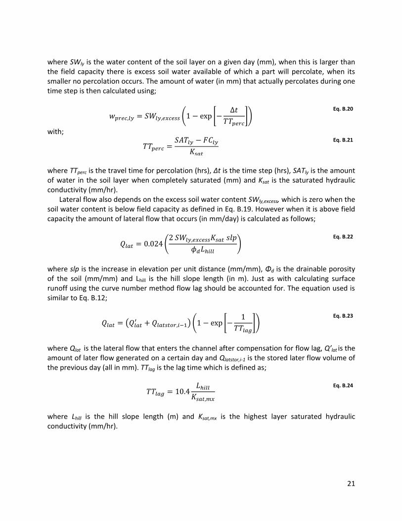
21

where SWly is the water content of the soil layer on a given day (mm), when this is larger than the field capacity there is excess soil water available of which a part will percolate, when its smaller no percolation occurs. The amount of water (in mm) that actually percolates during one time step is then calculated using;

Eq. B.20

with;

Eq. B.21

where TTperc is the travel time for percolation (hrs), Δt is the time step (hrs), SATly is the amount of water in the soil layer when completely saturated (mm) and Ksat is the saturated hydraulic conductivity (mm/hr).

Lateral flow also depends on the excess soil water content SWly,excess, which is zero when the soil water content is below field capacity as defined in Eq. B.19. However when it is above field capacity the amount of lateral flow that occurs (in mm/day) is calculated as follows;

Eq. B.22

where slp is the increase in elevation per unit distance (mm/mm), Φd is the drainable porosity of the soil (mm/mm) and Lhill is the hill slope length (in m). Just as with calculating surface runoff using the curve number method flow lag should be accounted for. The equation used is similar to Eq. B.12;

Eq. B.23

where Qlat is the lateral flow that enters the channel after compensation for flow lag, Q’lat is the amount of later flow generated on a certain day and Qlatstor,i-1 is the stored later flow volume of the previous day (all in mm). TTlag is the lag time which is defined as;

Eq. B.24

where Lhill is the hill slope length (m) and Ksat,mx is the highest layer saturated hydraulic conductivity (mm/hr).

22

Table B - 4: Soil water related parameters in SWAT

Parameter Definition Unity Type

SOL_AWC Available water capacity - Soil parameter

SOL_K Saturated hydraulic conductivity mm/hr Soil parameter

IWATABLE High water table code (0: no water table in soil profile, 1: seasonal water table in soil profile)

- HRU parameter

SLSOIL Hill slope length m HRU parameter

LAT_TIME Lateral flow travel time days Management parameter

GDRAIN Drain tile lag time hrs Management parameter

B.2.4. Ground Water

Ground water is stored in the saturated zone below the soil storage. In SWAT ground water is divided over two aquifers; a shallow aquifer and a deep aquifer. The water balance for the shallow aquifer is defined as follows;

Eq. B.25

where ΔVaq,sh is the change in water content of the shallow aquifer over time step Δt, wrchrg,sh is the amount of water entering the shallow aquifer (recharge, derived from wseep and transmission losses due to surface runoff), Qgw is the ground water outflow into the main channel (also referred to as return flow or base flow), wrevap is the amount of water moving back into the soil zone (capillary rise) and wpump is the amount of water abstracted from the shallow aquifer by pumping, all values are in mm per time step except for ΔVaq,sh which is in mm.

Recharge is calculated for both deep and shallow aquifer and depends on ground water delay time and seepage. To determine the amount of recharge into the shallow aquifer the recharge to the deep aquifer needs to be subtracted from the total recharge using a deep aquifer percolation coefficient βdeep;

Eq. B.26

The base flow or groundwater flow to the stream is determined using a non steady-state equation. Base flow is zero when the water in the aquifer is below a certain threshold, but once it passes this threshold it is calculated using an equation based on the recharge rate and a base flow recession constant;

Eq. B.27

where Qgw,I is the base flow on day i, Qgw,i-1 is the base flow on the previous day (both in mm) , Δt is the daily time step, αgw is the base flow recession constant, aqsh is the amount of water

23

stored in the shallow aquifer at the beginning of day i and aqshthr,q is the threshold above which base flow occurs.

When water moves back from the shallow aquifer to the unsaturated zone it is called revap. Revap is calculated using the following algorithm;

Eq. B.28

where wrevap is the amount of water that moves to the soil zone and wrevap,mx is the maximum amount of water that can move to the soil zone (both in mm). The maximum amount of revap is determined by;

Eq. B.29

where βrev is the revap coefficient and E0 is the potential evaporation in mm/day.

The water balance for the deep aquifer is somewhat more simplistic;

Eq. B.30

where aqdp,i and aqdp,i-1 are the amount of water stored on day i and the previous day, wdeep is the amount of water percolation from the shallow aquifer into the deep aquifer (βdeepwrchrg) and wpump,dp is the amount of water abstracted from the deep aquifer by pumping, all variables are in mm.

Table B - 5: Groundwater related parameters in SWAT

Parameter Definition Unity Type

GW_DELAY Delay time for aquifer recharge days Groundwater parameter

GWQMN Threshold water level in shallow aquifer for base flow to occur

mm Groundwater parameter

ALPHA_BF Base flow recession constant - Groundwater parameter

REVAPMN Threshold level in shallow aquifer for revap to occur mm Groundwater parameter

GW_REVAP Revap coefficient - Groundwater parameter

RCHRG_DP Aquifer percolation coefficient - Groundwater parameter

GW_SPYLD Specific yield of shallow aquifer m/m Groundwater parameter

B.3. Water routing

The water that flows into the channel according to the calculations made into the previous sections is routed to the downstream basin. Two methods are available in SWAT to route the water; the variable storage method and the Muskinghum method. Only the variable storage method will be explained here as this is the method that will be used. SWAT uses a trapezoidal profile to present the channel cross-section as is shown in Figure B - 1.

24

Figure B - 1: Trapezoidal profile used by SWAT

The relation between water depth and flow rate (in m3/s) is as follows;

Eq. B.31

where Ach is the cross sectional area (m2), Rch is the hydraulic radius (m), slpch is the slope of the channel (m/m) and n is Manning’s roughness coefficient. To calculate the amount of water that flows out of the downstream boundary of the channel the variable storage routing method is used. The method is based around a water balance that represents the fluxes in and out of the channel;

Eq. B.32

where qin,1 and qin,2 are the flows into the channel at the beginning and end of time step Δt and qout,1 and qout,2 are the flows out of the channel at the beginning and end of time step Δt. Vstored,1 and Vstored,2 are the volumes of water stored in the channel at the beginning and end of time step Δt. After some transformations the equation used to calculate the amount of water that flows out is obtained;

Eq. B.33

with;

Eq. B.34

where Vout,2 is volume of water that flows out (m3), SC is the storage coefficient, Vin is the

volume of water (m3) that flows in on average during time step Δt, and TT is the travel time that the water needs to flow through the channel (s). However, the water balance also contains some other elements such as transmission losses, evaporation losses and bank storage. These are included in a more detailed water balance;

Eq. B.35

25

where ΔVch is the change in water volume stored in the channel over time step Δt. Vin is the water volume flowing in the reach from either the land phase (surface runoff, lateral flow, return flow) or an upstream basin. Vout is the water volume flowing out of the reach to the next basin. tloss represents transmission losses through the bed of the channel (into the shallow aquifer), Ech represents evaporation losses, div represents either losses or additions due to diversion of the water (f.e. for irrigation) and Vbnk represents water that is returned to the reach via bank storage, all values are in m3 per time step except for ΔVch which is in m3 H2O. Transmission losses, evaporation losses and bank storage are calculated as follows;

Eq. B.36

Eq. B.37

Eq. B.38

where Kch is the hydraulic conductivity of the channel (mm/hr), TT is the flow travel time (hr), Pch is the wetted perimeter (m) and Lch is the channel length (km). coefev is a channel evaporation coefficient, Eo is the potential evaporation (mm), W is the channel width at the water level (m) and frΔt is the fraction of the time step in which water is flowing through the channel. bnk (m3 H2O) is the total amount of water in bank storage and αbnk is the bank flow recession constant.

Table B - 6: Water routing related parameters in SWAT

Parameter Definition Unity Type

CH_W(2) Channel width at top of bank m Routing parameter

CH_D Bankful channel depth m Routing parameter

CH_L(2) Length of main channel km Routing parameter

CH_S(2) Average slope along channel length m/m Routing parameter

CH_N(2) Manning’s roughness coefficient for the main channel - Routing parameter

CH_K(2) Effective hydraulic conductivity of channel mm/hr Routing parameter

IRTE Channel water routing method (0: variable storage method, 1: Muskingum method)

- Basin parameter

EVRCH Reach evaporation adjustment factor - Basin parameter

ALPHA_BNK Bank flow recession constant - Routing parameter

TRNSRCH Fraction of transmission losses partitioned to deep aquifer

- Basin parameter

B.4. ArcSWAT

The extension of SWAT that will be used is ArcSWAT 2009.93.7b which is the SWAT 2009 interface for ESRI ArcGIS 9.3.1 SP2. The advantage of this interface is that it allows for relatively easy processing of spatial data sets. In Figure B - 2 an overview of the general steps one has to perform before one can run the model is shown along with the input that is required by ArcSWAT for each step.

The first step requires a DEM for basin delineation. To improve delineation, a predefined river network and a predefined set of watersheds may be used. Once the basin is delineated

26

the HRUs need to be classified. They are based on land use, soil characteristics and slope classes. The slope classes can be derived from the DEM while the land use and soil maps have to be loaded into the program, together with lookup tables that convert the parameters in those maps to SWAT compatible parameters. Additional soil classes will be loaded into the SWAT database because the soils in the soil data base are only classified for the USA. The next step is to load the weather data. Measured rainfall data are available and can be loaded directly into SWAT. For the other types of weather data (min/max temperatures, solar radiation, relative humidity and wind speed) less data are available and a weather generator has to be used. The input for this weather generator are parameters derived from the data that is available, these parameters are related to a number of weather stations and stored in the SWAT data base. Additionally a file with the locations of the weather stations is loaded.

Once these steps of basin delineation, HRU analysis and weather data input are completed the model is ready to run. The only thing left to do is to try and improve estimates for some of the parameters for which proper estimates can be made. The parameters that are unknown can be estimated by using the automatic calibration provided in the ArcSWAT interface. Various types of output can be selected and will be stored in a database. This output can be provided on a daily, monthly or yearly basis to save calculation time.

In Figure B - 3 an overview of the calculation steps that SWAT performs within one sub-basin is shown. The model starts with reading or generating precipitation and maximum and minimum temperatures. This step is followed by generation of solar radiation, wind speed and relative humidity since these depend on precipitation and temperatures. Based on these meteorological variables soil temperatures are calculated and consequently snowfall and snowmelt, of which the latter two are not relevant in this study case as there is no snowfall in this area of the world. When rainfall is larger than zero a part of the precipitation will either infiltrate or will be converted to surface runoff. When the infiltration is so high that there is no surface runoff the components of the water balance will be updated, else another step is taken where the properties of the surface runoff (peak rate, transmission losses) are calculated. When rainfall is not larger than zero there is no surface runoff or infiltration and the remaining components of the water balance will be updated directly.

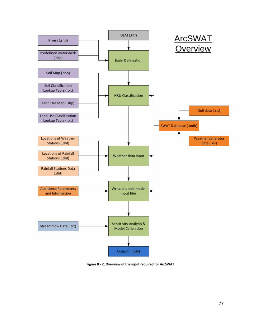
27

Soil Map (.shp)

Basin Delineation

HRU Classification

Rainfall Stations Data (.dbf)

Soil Classification Lookup Table (.txt)

Locations of Weather Stations (.dbf)

Land Use Map (.shp)

Weather data inputLocations of Rainfall

Stations (.dbf)

SWAT Database (.mdb)

DEM (.tiff)

Land Use Classification Lookup Table (.txt)

Stream flow Data (.txt)

Write and edit model input files

Sensitivity Analysis & Model Calibration

Additional Parameters and Information

Weather generator data (.xls)

Soil data (.xls)

ArcSWAT

Overview

Output (.mdb)

Rivers (.shp)

Predefined watersheds (.shp)

Figure B - 2: Overview of the input required for ArcSWAT

28

Enter HRU/Subbasin command loop

Read or generate Precipitation and max/min temperatures

Generate solar radation, wind speed and relative humidity

Compute soil temperature

Compute snowfall and snowmelt

Rainfall + snowmelt > 0?

Compute surface runoff and infiltration

Surface runoff > 0?

Compute soil water routing, ET, crop growth,

pond and wetland balances, groundwater

flow and height

Compute peak rate, transmission losses,

sediment yield, nutrient and pesticide yields

Exit HRU/Subbasin command loop

Yes

No

Yes

No

Figure B - 3: HRU/Sub-basin Command Loop, based on Neitsch et al. (2011)

29

Appendix C – Land use/land cover map

Figure C - 1: Land use/land cover map of the Lake Naivasha basin assimilated by Odongo (2012) based on a vegetation map of

1973. Eight different LULC classes were used.

30

Appendix D – Soil Map & Parameters

D.1. Soil Map of the Lake Naivasha basin

Figure D - 1: Soil map of the Lake Naivasha basin; a detailed description of the units used to classify the soils can be found in

the Exploratory Soil Survey Report No. E1, Kenya Soil Survey, Nairobi 1982 (Sombroek et al., 1982)

31

D.2. Soil Parameters

The soil classifications used in the map of the Kenyan Soil Survey were transformed into SWAT parameters in combination with additional measurements performed in 2003. In Table D - 1 the SWAT soil parameter definitions are shown and in Table D - 2 though Table D - 5 the parameter values used in SWAT are shown for each layer. Three different soil layers have been defined (Muthuwatta, 2004; Tiruneh, 2003).

Table D - 1: SWAT Soil parameter definitions

Parameter Description Unity Range

SNAM Soil name (optional) - -

NLAYERS Number of soil layers - 1 - 10

HYDGRP Soil Hydrological group - A - D

SOL_ZMX Maximum rooting depth mm 0 - 3500

ANION_EXCL Fraction of porosity from which anions can be extracted (optional)

- 0.01 - 1

SOL_CRK potential or maximum crack volume (optional)

- 0 - 1

TEXTURE Texture of soil layer (optional) - -

SOL_Z (# layer) Depth from soil surface to bottom layer

mm 0 - 3500

SOL_BD (# layer) Moist bulk density g/cm3 0.9 - 2.5

SOL_AWC (# layer) Available water capacity of the soil layer (mm/mm soil)

- 0 - 1

SOL_K (# layer) Saturated hydraulic conductivity mm/hour 0 - 3000

SOL_CBN (# layer) Organic carbon content (% of soil weight)

% 0.05 - 10

CLAY (# layer) Clay content % 0 - 100

SILT (# layer) Silt content % 0 - 100

SAND (# layer) Sand content % 0 - 100

ROCK (# layer) Rock fragment content % 0 - 100

SOL_ALB (top layer) Moist soil albedo - 0 - 0.25

USLE_K (# layer) USLE equation soil erodability factor K

0.013 (metric ton m2 hr)/(m

3-

metric ton cm) 0 - 0.65

SOL_EC (# layer) Electric conductivity (optional) dS/m 0 - 100

32

Table D - 2: General soil characteristics

OBJECTID MUID SEQN SNAM S5ID CMPPCT NLAYERS HYDGRP SOL_ZMX ANION_EXCL SOL_CRK TEXTURE

1 R3 3 C 2000 0.5 0 soiltxt

2 Ux3 3 C 2500 0.5 0 soiltxt

3 H9 3 C 2000 0.5 0 soiltxt

4 L20 3 C 2500 0.5 0 soiltxt

5 Pi11 3 B 2200 0.5 0 soiltxt

6 H4 3 C 2100 0.5 0 soiltxt

7 Ux7 3 B 2200 0.5 0 soiltxt

8 H6 3 C 2400 0.5 0 soiltxt

9 LU2 3 C 2350 0.5 0 soiltxt

10 L22 3 D 2200 0.5 0.5 soiltxt

11 S1 3 C 2000 0.5 0 soiltxt

12 R1 3 C 2000 0.5 0 soiltxt

13 F7 3 C 2500 0.5 0 soiltxt

14 M2 3 C 2050 0.5 0 soiltxt

15 M9 3 C 1800 0.5 0 soiltxt

16 L21 3 C 2190 0.5 0 soiltxt

17 Ux5 3 C 2250 0.5 0 soiltxt

18 Pv6 3 B 2420 0.5 0 soiltxt

19 M1 3 C 1500 0.5 0 soiltxt

20 Lake_Naivasha 1 D 0 0 0 soiltxt

21 PI7 3 B 2300 0.5 0.2 soiltxt

22 Lava 3 D 2000 0.5 0 soiltxt

33

Table D - 3: Characteristics soil layer #1

OBJECTID SOL_Z1 SOL_BD1 SOL_AWC1 SOL_K1 SOL_CBN1 CLAY1 SILT1 SAND1 ROCK1 SOL_ALB1 USLE_K1 SOL_EC1

1 150 1.32 0.3 1 3 50 45 5 0.15 0.09 0.1 1

2 150 1.12 0.27 2300 3.57 50 35 15 0.1 0.1 0.01 1

3 100 1.33 0.26 2400 2.364 79 12 17 1.5 0.1 0.2 1

4 100 1.1 0.28 1230 2.5 60 25 15 1 0 0.1 1

5 100 1.24 0.3 2500 3.3 35 55 10 1.2 0.2 0.3 1

6 100 1.34 0.28 2300 2.03 35 34 31 5 0.2 2.1 1

7 100 1.35 0.275 2500 1.1 10 25 65 5 0.1 2.5 1

8 100 1.32 0.29 1800 1 55 15 30 1.5 0.1 0.35 1

9 100 1.25 0.28 1500 1 50 20 30 0.1 0.1 0.1 1

10 100 1.45 0.31 400 3.18 70 17 12 0.2 0.2 0 1

11 100 1.25 0.27 1800 5 56 30 14 1 0.1 0.1 1

12 100 1.24 0.285 1900 3.5 65 16 19 1 0.2 0.12 1

13 100 1.43 0.32 1850 8.07 55 30 15 6 0.3 0.2 1

14 100 1.32 0.3 1820 8.42 40 35 25 50 0.25 0.25 1

15 100 1.28 0.275 1750 7 41 37 22 20 0.2 0.1 1

16 100 1.385 0.29 1200 5.63 35 55 10 0.1 0.26 0.05 1

17 100 1.31 0.285 1300 1.88 50 35 15 2 0.2 0.15 1

18 100 1.09 0.25 2200 1.18 5 25 70 1 0.12 0.15 1

19 100 1.2 0.28 1300 1.3 57 23 20 9 0.2 0.2 1

20 0 0 0 0 0 0 100 0 0 0 0 0

21 100 1.24 0.26 2600 3.53 15 50 35 2 0.1 0.01 1

22 100 1.3 0.28 1860 0 0 85 15 50 0.23 0.5 1

34

Table D - 4: Characteristics soil layer #2

OBJECTID SOL_Z2 SOL_BD2 SOL_AWC2 SOL_K2 SOL_CBN2 CLAY2 SILT2 SAND2 ROCK2 SOL_ALB2 USLE_K2 SOL_EC2

1 800 1.5 0.25 30 1 50 45 5 1.5 0.15 0.09 1

2 1000 1.5 0.3 180 0.5 35 45 20 0.12 0.1 0.1 1

3 750 1.45 0.29 190 0.3 65 15 20 2 0.1 0.3 1

4 860 1.2 0.285 15 0.6 55 30 15 1 0 0.1 1

5 600 1.25 0.3 250 0.45 36 39 25 1.5 0.2 0.35 1

6 600 1.21 0.28 2300 0.45 38 37 25 5.1 0.2 2.2 1

7 1000 1.36 0.3 240 0.08 10 35 55 5.2 0.1 2.5 1

8 950 1.35 0.31 100 0.35 55 15 30 1.5 0.1 0.35 1

9 950 1.27 0.29 120 0.8 45 25 30 2.1 0.1 0.3 1

10 1100 1.5 0.35 20 0.85 65 22 12 0.2 0.2 0 1

11 970 1.3 0.28 50 0.76 50 35 15 1 0.1 0.15 1

12 1000 1.26 0.29 54 3.1 60 21 19 1.5 0.2 0.15 1

13 980 1.45 0.34 60 2.8 50 35 15 7 0.3 0.25 1

14 1010 1.35 0.32 55 3.1 38 36 26 50 0.25 0.25 1

15 750 1.29 0.29 70 2.9 38 38 24 25 0.2 0.15 1

16 860 1.4 0.3 10 1.4 34 56 10 0.1 0.26 0.05 1

17 780 1.33 0.289 9 0.6 45 40 15 2.5 0.2 0.15 1

18 900 1.1 0.28 1800 0.118 30 15 55 2 0.12 0.15 1

19 850 1.25 0.29 15 0.52 55 25 20 9 0.2 0.22 1

20

21 850 1.25 0.23 2000 0.14 20 60 20 2.1 0.1 0.01 1

22 500 1.35 0.28 120 0 0 90 10 60 0.23 0.5 1

35

Table D - 5: Characteristics soil layer #3

OBJECTID SOL_Z3 SOL_BD3 SOL_AWC3 SOL_K3 SOL_CBN3 CLAY3 SILT3 SAND3 ROCK3 SOL_ALB3 USLE_K3 SOL_EC3

1 800 1.5 0.3 30 0 50 45 5 1.5 0.15 0.09 1

2 2500 1.5 0.3 150 0 30 50 20 0.15 0.1 0.12 1

3 2000 1.45 0.29 150 0 60 15 25 3 0.1 0.3 1

4 2500 1.2 0.285 15 0 55 30 15 1 0 0.1 1

5 2200 1.25 0.3 180 0 38 42 20 1.5 0.2 0.35 1

6 2100 1.21 0.27 2400 0 36 39 25 5.1 0.2 2.2 1

7 2200 1.36 0.3 200 0 10 35 55 5.2 0.1 2.5 1

8 2400 1.35 0.31 50 0 40 30 30 1.5 0.25 0.35 1

9 2350 1.27 0.29 30 0 45 25 30 2.1 0.1 0.3 1

10 2200 1.5 0.35 10 0 65 22 12 0.2 0.2 0 1

11 970 1.3 0.28 15 0 50 35 15 1 0.1 0.15 1

12 2000 1.26 0.29 12 0 55 25 20 1.5 0.2 0.2 1

13 2500 1.45 0.34 11 0 50 35 15 7 0.3 0.25 1

14 2050 1.35 0.32 25 0 38 36 26 50 0.25 0.25 1

15 1800 1.29 0.29 25 0 38 38 24 25 0.2 0.15 1

16 2190 1.4 0.3 10 0 34 56 10 0.1 0.26 0.05 1

17 2250 1.33 0.289 9 0 45 40 15 2.5 0.2 0.15 1

18 2420 1.1 0.28 200 0 30 15 55 2 0.12 0.15 1

19 1500 1.25 0.29 15 0 55 25 20 9 0.2 0.22 1

20

21 2300 1.25 0.23 2000 0 20 60 20 2.1 0.1 0.01 1

22 2000 2.65 0.02 2 0 0 100 0 90 0.23 0.5 1

36

Appendix E – Rainfall Data

E.1. Available rain stations around Lake Naivasha

In Figure E - 1 the locations of the rain stations in and around the Lake Naivasha basin are shown. By using the gauge ID (GID) the name and characteristics of each station can be looked up in Table E - 1.

Figure E - 1: Map containing the locations of rain stations in and around the Lake Naivasha basin

37

Table E - 1: Rain stations in and around the Lake Naivasha basins (source: Kenya Metrological Department (2004) and data collected by ITC)

GID STATION_NAME STATION_ID X_COORD Y_COORD PERCENTAGE OF MISSING DATA

ELEVATION

1 NAIVASHA D.O. 9036002 214500.0 9920200.0 5% 1923

2 KEDONG VALLEY, MAAI MAHIU 9036011 232895.8 9891262.9 75% 2021

3 N. KINANGOP FOREST STATION 9036025 236545.6 9935511.5 2% 2617

4 GILGIL RAILWAY STATION. 9036034 202500.0 9945300.0 29% 1995

5 KANGARI FARM , NAIVASHA 9036059 219843.2 9928092.2 71% 2233

6 KIRITA FOREST STATION 9036061 236570.6 9891265.5 27% 2390

7 NAIVASHA KONGONI FARM 9036062 195794.8 9909601.7 59% 1882

8 NAIVASHA NANGA GERRI 9036065 225418.9 9915152.1 64% 2369

9 MWEIGA ESTATE 9036072 268163.1 9961292.3 32% 1900

10 NAIVASHA K.C.C. LTD. 9036073 209500.0 9926205.7 38% 1900

11 TECHNOLOGY FARM, NAKURU 9036076 167914.4 9966798.7 29% 1895

12 NAIVASHA VET.EXPT. STATION 9036081 213000.0 9928088.5 27% 1923

13 KARAMENO SHOPPING CENTRE N/MORU 9036085 251455.9 9985289.6 59% 2058

14 NAIVASHA MARULA ESTATE 9036109 208500.0 9929100.0 18% 1894

15 CHOKEREREIA F.C. SOCIETY 9036129 205018.6 9952093.3 70% 2234

16 ELEMENTAITA,SOYSAMBU ESTATE 9036147 187500.0 9948325.1 26% 1841

17 GILGIL, KIKOPEY RANCH 9036150 184633.5 9948323.6 46% 1849

18 SUBUKIA PYRETHRUM NURSERY 9036151 184623.1 9996348.4 35% 2090

19 S.KINANGOP NJABINI F.T.C. 9036152 240500.0 9918700.0 32% 2508

20 KIJABE RAILWAY STATION 9036162 230997.6 9898562.4 41% 2336

21 S. KINANGOP FOREST STATION 9036164 242120.7 9920692.0 33% 2542

22 ABERDARE PARK FORT JERUSALEM 9036174 240329.2 9942813.5 86% 3125

23 NAIVASHA KORONGO FARM 9036179 197572.2 9917016.2 51% 1889

24 NAIVASHA KARATI SCHEME 9036183 227310.0 9918914.3 77% 2531

25 KINANGOP SASUMUA DAM 9036188 240340.8 9917040.8 32% 2475

26 NEW GAKOE FARM (NAKURU) 9036198 184626.5 9970454.8 69% 1944

27 NAIVASHA LONGONOT FARM 9036214 208715.8 9909610.3 56% 1904

28 ELEMENTAITA NDERIT RANGER POST 9036227 180743.3 9953655.1 35% 1829

29 NAKURU LANET POLICE POST 9036236 182533.3 9967302.7 42% 1898

30 GETA FOREST STATION 9036241 233394.0 9947946.0 38% 2588

31 DUNDORI FOREST STATION 9036243 191979.1 9972337.6 30% 2345

32 KIENI FOREST STATION 9036244 240347.1 9905979.6 31% 2513

33 MENENGAI FOREST STATION 9036252 175267.0 9972333.9 34% 2223

34 THOME FARMERS NO.2 9036253 197564.8 9929961.6 58% 2352

35 AVONDALE ESTATE SUBUKIA 9036256 190193.7 9996348.5 41% 2138

36 GATARE FOREST STATION 9036259 251474.6 9920696.6 38% 2536

37 NAKURU METEOROLOGICAL STATION 9036261 177161.6 9970453.1 39% 1910

38 OLARAGWAI FARM NAIVASHA 9036262 215500.0 9928090.4 38% 2019

39 N. KINANGOP MAWINGO SCHEME 9036264 223622.8 9944687.8 53% 2403

40 MUTUBIO GATE (A.N.PARK) 9036272 239876.0 9942226.0 52% 3191

41 MAGURA RIVER 9036277 244002.9 9946575.6 96% 3017

42 RIUNGE HILL 9036278 245893.2 9955756.7 96% 3159

43 CULVERT CAMP 9036279 251460.8 9957638.5 95% 2610

38

44 CHANIA RIVER,ABERD. NAT. PARK 9036280 245894.9 9950226.3 96% 2989

45 NAIVASHA W.D.D. 9036281 216172.6 9918908.1 45% 1996

46 LONGONOT AKIRA RANCH 9036285 206946.9 9891243.3 87% 1735

47 WANJOHI CHIEF'S CAMP 9036289 223136.0 9962352.0 55% 2437

48 MALEWA FARMER'COOP. SOC. 9036290 216155.3 9959398.7 65% 2332

49 NGECHA NEW FARMERS CO-OP. 9036294 206913.0 9950213.1 91% 2170

50 KURASE HILL ABERDARE PARK 9036296 240323.0 9963166.1 97% 3350

51 KANGUI SECONDARY SCHOOL 9036307 203117.1 9987055.1 76% 2515

52 NGETHU WATER SUPPLY 9036308 266295.5 9898584.6 56% 1792

53 MITI MINGI FARM 9036309 177172.0 9941016.9 88% 1893

54 KAMIRITHU FANCY FARM 9036310 169698.8 9961265.8 70% 1921

55 CHAMATA GATE 9036312 225396.1 9977875.4 56% 2797

56 CHEBUSWA HILL 9036313 232858.9 9974226.1 98% 3274

57 SAKUTIEK C.C. OUTPOST 9036317 182763.8 9905940.9 92% 2715

58 MUGUNDA PRIMARY SCHOOL 9036319 243994.9 9981528.2 71% 2350

59 NAISHI RANGER'S POST 9036320 175273.9 9950201.1 79% 1786

60 CRESCENT ISLAND 9036322 210500.0 9915137.6 67% 1893

61 KIANGANYE FARM ICHICHI 9036323 257041.3 9922579.5 60% 2344

62 OLCHORO AGRI. OFFICE 9036331 167944.8 9907811.1 72% 2624

63 TUMAINI N.Y.S. CAMP 9036336 197549.7 9971400.0 65% 2539

64 SURURU FOREST STATION 9036337 169709.7 9935479.8 78% 2531

65 OLKARIA GEOTHERMAL STATION 9036343 199477.2 9900420.8 75% 2017

66 GILGIL KWETU FARM 9036999 199826.0 9961909.0 0% 2391

67 KIJABE FARM 9036666 211924.8 9914724.7 48% 1907

E.2. Correlation analysis

To decide whether it is more effective to interpolate on a monthly or daily basis a correlation analysis between the 67 rain stations was performed. The correlation coefficient used to indicate how well stations correlate is calculated as follows (Davis, 2002);

Eq. E.1

where Xi and Yi are the rainfall records (monthly or daily) of stations X and Y. The goal of this analysis is to determine if correlations are higher on a monthly scale than on a daily scale. If this is indeed the case then monthly values will be used to scale daily values because the monthly values are more reliable.

All 67 available rainfall gauging stations were correlated with each other, first using daily data and then using monthly data. Only the original data was used, this meant that not all stations could be compared because a few stations were operational only in periods where other stations were closed. Average correlations for each station are shown in Table E - 2, it is clear that on a monthly scale correlations are much higher and therefore it is appropriate to use monthly interpolated data to scale daily interpolated data.

39

Table E - 2: Correlations between rain stations ID Daily Correlations Monthly Correlations

1 0.24 0.56

2 0.31 0.71

3 0.22 0.60

4 0.20 0.56

5 0.28 0.67

6 0.26 0.59

7 0.24 0.57

8 0.25 0.59

9 0.17 0.50

10 0.23 0.61

11 0.19 0.55

12 0.21 0.56

13 0.18 0.48

14 0.22 0.61

15 0.26 0.61

16 0.22 0.55

17 0.21 0.56

18 0.17 0.51

19 0.24 0.59

20 0.25 0.60

21 0.25 0.61

22 0.23 0.45

23 0.26 0.64

24 0.22 0.43

25 0.27 0.60

26 0.22 0.63

27 0.23 0.62

28 0.21 0.59

29 0.21 0.54

30 0.20 0.53

31 0.17 0.47

32 0.25 0.55

33 0.21 0.57

34 0.22 0.61

35 0.26 0.59

36 0.24 0.57

37 0.22 0.55

38 0.25 0.60

39 0.21 0.55

40 0.24 0.55

41 0.11 0.35

42 0.13 0.28

43 0.14 0.39

44 0.11 0.11

45 0.24 0.61

40

46 0.22 0.55

47 0.21 0.50

48 0.18 0.54

49 0.20 0.64

50 0.10 0.34

51 0.15 0.45

52 0.21 0.55

53 0.18 0.57

54 0.12 0.24

55 0.19 0.47

56 0.12 0.05

57 0.17 0.53

58 0.15 0.36

59 0.18 0.46

60 0.24 0.56

61 0.23 0.57

62 0.20 0.50

63 0.18 0.50

64 0.21 0.60

65 0.23 0.53

66 0.17 0.57

67 0.25 0.59

41

Appendix F – Weather data

In Figure F - 1 the locations of the weather stations generated for usage in SWAT are shown. For each station the parameters required by the weather generator have been calculated; they are shown in Table F - 1.

Figure F - 1: Map containing the locations of the weather stations in the Lake Naivasha basin as they have been

generated for usage in SWAT

42

Table F - 1: Weather generator parameters used in SWAT

Weather generator parameters

OBJECTID 1 2 3

STATION LAKE PLATEAU ABERDARE

WLATITUDE 36.29 36.48 36.66

WLONGITUDE -0.83 -0.50 -0.52

WELEV 1912 2336 3199

RAIN_YRS 60.00 60.00 60.00

TMPMX1 27.70 25.34 15.02

TMPMX2 28.30 26.29 15.58

TMPMX3 27.30 25.47 15.09

TMPMX4 25.10 24.26 14.38

TMPMX5 23.80 23.43 13.88

TMPMX6 23.00 21.93 12.99

TMPMX7 22.50 20.48 12.14

TMPMX8 22.90 21.40 12.68

TMPMX9 24.50 22.79 13.50

TMPMX10 25.60 23.57 13.97

TMPMX11 24.70 23.30 13.81

TMPMX12 25.80 24.55 14.55

TMPMN1 8.10 2.78 1.88

TMPMN2 8.20 2.65 1.80

TMPMN3 9.80 6.12 4.15

TMPMN4 11.50 6.95 4.71

TMPMN5 11.30 5.16 3.50

TMPMN6 9.90 3.25 2.20

TMPMN7 9.30 4.76 3.23

TMPMN8 9.40 5.54 3.76

TMPMN9 8.80 3.64 2.47

TMPMN10 9.10 4.99 3.38

TMPMN11 9.30 7.03 4.77

TMPMN12 8.70 3.76 2.55

TMPSTDMX1 0.32 1.68 1.56

TMPSTDMX2 0.53 1.67 1.55

TMPSTDMX3 0.94 2.10 1.94

TMPSTDMX4 1.01 1.78 1.65

TMPSTDMX5 0.48 2.19 2.03

TMPSTDMX6 0.73 1.82 1.69

TMPSTDMX7 0.62 2.04 1.89

TMPSTDMX8 0.62 2.05 1.90

43

TMPSTDMX9 0.52 1.97 1.82

TMPSTDMX10 0.74 2.00 1.85

TMPSTDMX11 0.61 1.89 1.75

TMPSTDMX12 0.62 1.87 1.73

TMPSTDMN1 1.28 2.68 2.26

TMPSTDMN2 0.96 3.33 2.81

TMPSTDMN3 1.63 2.95 2.49

TMPSTDMN4 1.20 2.02 1.70

TMPSTDMN5 0.90 2.79 2.35

TMPSTDMN6 1.04 2.17 1.83

TMPSTDMN7 0.74 2.91 2.45

TMPSTDMN8 0.83 2.71 2.28

TMPSTDMN9 1.50 1.95 1.64

TMPSTDMN10 0.90 2.06 1.74

TMPSTDMN11 1.01 2.62 2.21

TMPSTDMN12 0.97 2.83 2.39

PCPMM1 37.04 44.01 49.73

PCPMM2 37.95 39.35 52.47

PCPMM3 62.05 67.39 85.04

PCPMM4 109.68 154.58 157.15

PCPMM5 82.14 142.96 152.55

PCPMM6 45.65 83.42 96.20

PCPMM7 33.76 68.12 68.80

PCPMM8 45.12 84.85 90.81

PCPMM9 42.84 74.55 101.32

PCPMM10 57.70 87.29 105.69

PCPMM11 71.99 86.95 105.26

PCPMM12 47.41 55.84 63.49

PCPSTD1 4.48 4.44 4.43

PCPSTD2 4.57 3.87 5.02

PCPSTD3 6.11 4.56 6.11

PCPSTD4 7.97 8.99 8.12

PCPSTD5 7.05 8.17 8.02

PCPSTD6 4.86 6.51 5.89

PCPSTD7 4.18 4.71 5.18

PCPSTD8 4.68 5.92 5.75

PCPSTD9 4.37 5.02 5.94

PCPSTD10 5.14 4.99 6.32

PCPSTD11 5.43 4.43 5.77

PCPSTD12 4.08 5.50 5.20

44

PCPSKW1 4.89 4.32 4.20

PCPSKW2 6.66 4.32 4.35

PCPSKW3 5.37 4.50 3.72

PCPSKW4 3.71 2.46 2.39

PCPSKW5 4.69 2.58 2.16

PCPSKW6 5.90 3.38 2.85

PCPSKW7 6.50 3.08 4.56

PCPSKW8 6.50 3.79 3.44

PCPSKW9 4.36 2.79 2.59

PCPSKW10 5.09 3.21 3.25

PCPSKW11 4.39 2.48 2.39

PCPSKW12 4.61 7.33 4.23

PR_W1_1 0.13 0.12 0.11

PR_W1_2 0.15 0.10 0.14

PR_W1_3 0.21 0.15 0.20

PR_W1_4 0.32 0.32 0.35

PR_W1_5 0.25 0.36 0.30

PR_W1_6 0.16 0.32 0.24

PR_W1_7 0.12 0.27 0.21

PR_W1_8 0.17 0.28 0.25

PR_W1_9 0.20 0.28 0.27

PR_W1_10 0.21 0.28 0.27

PR_W1_11 0.27 0.30 0.31

PR_W1_12 0.19 0.14 0.17

PR_W2_1 0.47 0.56 0.52

PR_W2_2 0.48 0.59 0.50

PR_W2_3 0.49 0.52 0.54

PR_W2_4 0.63 0.74 0.68

PR_W2_5 0.52 0.68 0.63

PR_W2_6 0.46 0.55 0.60

PR_W2_7 0.44 0.63 0.52

PR_W2_8 0.43 0.62 0.57

PR_W2_9 0.39 0.61 0.61

PR_W2_10 0.50 0.63 0.59

PR_W2_11 0.57 0.71 0.63

PR_W2_12 0.42 0.50 0.53

PCPD1 6.21 6.41 5.64

PCPD2 6.20 5.70 6.16

PCPD3 9.03 7.46 9.44

PCPD4 14.07 16.54 15.67

45

PCPD5 10.64 16.50 13.99

PCPD6 6.93 12.41 11.33

PCPD7 5.58 13.04 9.43

PCPD8 7.22 13.19 11.37

PCPD9 7.31 12.58 12.11

PCPD10 9.20 13.40 12.40

PCPD11 11.73 15.14 13.70

PCPD12 7.58 6.92 8.12

RAINHHMX1 48.00 50.00 47.00

RAINHHMX2 56.00 53.00 44.00

RAINHHMX3 53.00 60.00 53.00

RAINHHMX4 62.00 71.00 110.00

RAINHHMX5 55.00 51.00 57.00

RAINHHMX6 63.00 61.00 40.00

RAINHHMX7 62.00 78.00 61.00

RAINHHMX8 65.00 70.00 77.00

RAINHHMX9 53.00 42.00 56.00

RAINHHMX10 58.00 71.00 56.00

RAINHHMX11 50.00 47.00 44.00

RAINHHMX12 47.00 59.00 78.00

SOLARAV1 23.14 19.50 10.65

SOLARAV2 22.64 19.54 10.67

SOLARAV3 22.09 20.04 10.94

SOLARAV4 20.13 17.20 9.39

SOLARAV5 20.00 15.86 8.66

SOLARAV6 19.62 16.61 9.07

SOLARAV7 18.91 13.39 7.31

SOLARAV8 20.33 15.19 8.29

SOLARAV9 21.76 18.07 9.87

SOLARAV10 22.05 19.58 10.69

SOLARAV11 19.75 17.57 9.60

SOLARAV12 22.51 18.95 10.35

DEWPT1 0.00 0.00 0.00

DEWPT2 0.00 0.00 0.00

DEWPT3 0.00 0.00 0.00

DEWPT4 0.00 0.00 0.00

DEWPT5 0.00 0.00 0.00

DEWPT6 0.00 0.00 0.00

DEWPT7 0.00 0.00 0.00

DEWPT8 0.00 0.00 0.00

46

DEWPT9 0.00 0.00 0.00

DEWPT10 0.00 0.00 0.00

DEWPT11 0.00 0.00 0.00

DEWPT12 0.00 0.00 0.00

WNDAV1 0.00 0.00 0.00

WNDAV2 0.00 0.00 0.00

WNDAV3 0.00 0.00 0.00

WNDAV4 0.00 0.00 0.00

WNDAV5 0.00 0.00 0.00

WNDAV6 0.00 0.00 0.00

WNDAV7 0.00 0.00 0.00

WNDAV8 0.00 0.00 0.00

WNDAV9 0.00 0.00 0.00

WNDAV10 0.00 0.00 0.00

WNDAV11 0.00 0.00 0.00

WNDAV12 0.00 0.00 0.00

47

Appendix G – River gauging stations

G.1. Locations of river gauging stations

Figure G - 1: Map containing the river gauging stations (RGS) in the Lake Naivasha basin

48

G.2. Schematic overview of river gauging stations

Lake

Naivasha

Mount Kipipiri

Kinangop Plateau

Ab

erd

are

s

2GB0708

2GB05

2GA01/05

2GA03

2GB04

2GB01

2GA06

2GB03

2GC05

2GC04

2GC07

2GC10

2GD02 2GD07

Gilg

il

Male

wa

Gilg

il

Little

Gilg

il

Turasha

Ma

lew

a

Wanjohi

Malewa

Mkungi

Kitiri

Turasha

Karati

Figure G - 2: Schematic overview of the main rivers and gauging stations in the Lake Naivasha basin

49

G.3. Rating Curve Analysis

The rating curves are developed according to the method described in Chapter 4. However, first the measured discharge-height (Q-H) data were inspected for outliers. In total five outliers were found and removed from the data set, they are explained in Table G - 1.

Table G - 1: Outliers in Q-H data

Station Date H [m] Q [m3/s] Explanation

2GA01 06-06-2010 0.48 1.622 Different gauging method, possibly taken at a different location than the original one

2GC04 01-06-2010 1.50 3.590 Different gauging method, highest water level with a relatively low discharge

2GC05 06-05-1977 0.94 0.390 Judged as outlier after visual inspection

2GC05 23-10-1985 0.63 0.460 Judged as outlier after visual inspection

2GC07 27-02-1988 0.12 2.401 Smallest water level with largest discharge

As stated in Chapter 4 the least square method was used as an objective function to

optimise the coefficients of the rating curve;

Eq. G.1

where Qobs,t is the measured discharge measured at moment t using the velocity-area method and Qcalc,t is calculated discharge calculated using the water level measured at moment t. T is the total number of observations. The resulting rating curve coefficients are shown in Table G - 2. To indicate the goodness-of-fit of the rating curves to the data the coefficient of determination (R2) was calculated for each station.

Eq. G.2

The results are shown in Figure G - 3 up to Figure G - 6. Most rating curves fit fairly well with the exception of 2GA06 which does not follow the expected trend of a rating curve. This is most likely caused by large changes in the stream over time. Because of this the data of 2GA06 cannot be used. 2GA05, 2GB07 and 2GC10 also do not fit very well but their R2 is at least above 0.50 and the shape of the curve follows the expected trend. The other stations all have an R2

over 0.80 which can be considered a good fit.

50

Table G - 2: Rating curve coefficients for Q = a(H-b)^c Station Coefficient a Coefficient b Coefficient c

2GA01 1.15 0.10 1.99

2GA03 2.08 0.00 1.65

2GA05 1.37 0.20 1.20

2GA06 0.05 0.00 0.40

2GB01 28.26 0.00 1.77

2GB03 5.16 0.00 2.23

2GB04 7.19 0.00 1.67

2GB05 7.62 0.29 1.70

2GB07 3.63 0.00 2.85

2GB08 9.82 0.00 2.52

2GC04 13.55 0.00 2.16

2GC05 4.47 0.00 1.52

2GC07 4.04 0.00 3.63

2GC10 1.65 0.02 2.50

2GD02 7.72 0.01 2.87

2GD07 5.68 0.09 2.18

51

Figure G - 3: Rating Curves 2GA RGS

52

Figure G - 4: Rating Curves 2GB RGS

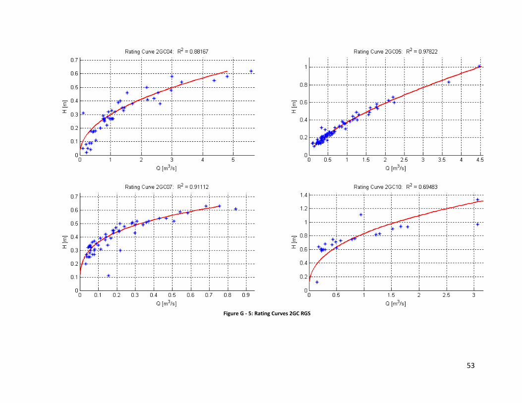
53

Figure G - 5: Rating Curves 2GC RGS

54

Figure G - 6: Rating Curves 2GD RGS

55

Appendix H – Sensitivity analysis

A sensitivity analysis is performed for each basin used in the study. The sensitivity analysis tool provided in the ArcSWAT interface is used (van Liew & Veith, 2009). The methods and parameters used in the analysis are explained in Chapter 4. The sensitivity analysis provides two methods to test sensitivity, both methods were applied. The first method calculates sensitivity in terms of change in average flow. The second method first calculates the objective function by comparing with observed data and the measures the change in this objective function when changing a parameter. The results of both methods are shown in this appendix. In Table H - 1 an overview of the results of the sensitivity analysis, when using change in average flow as a criterion, are shown. As can be seen sensitivities vary per basin but no specific pattern can be observed. In Table H - 2 the results of the sensitivity analysis when using change in objective function as a criterion for sensitivity. The difference between the two testing methods is summarized in Table H - 3. For each sensitivity analysis the parameters have been ranked and the average rank for each parameter for all basins is calculated.

56

Table H - 1: Rates of average change in average flow per parameter per basin

Parameters 2GB01(1) 2GB01(3) 2GB05(3) 2GC04(3) 2GB01(7) 2GB05(7) 2GB0708(7) 2GB04(7) 2GC04(7) 2GC05(7) 2GC07(7)

Alpha_Bf 2.99E-02 1.71E-02 3.44E-02 3.29E-02 1.82E-02 2.61E-02 3.00E-02 3.04E-02 2.68E-02 2.63E-02 2.17E-02

Blai 1.96E-01 1.42E-02 2.67E-01 1.76E-01 1.18E-02 1.16E-01 1.42E-01 8.95E-02 1.34E-01 8.68E-02 7.46E-02

Canmx 3.17E-01 9.95E-03 3.26E-01 7.29E-01 1.02E-02 1.39E-01 1.71E-01 6.06E-01 2.23E-01 4.62E-01 4.29E-01

Ch_K2 3.76E-02 5.08E-03 4.16E-02 3.32E-02 4.86E-03 1.48E-02 2.90E-02 1.91E-02 1.90E-02 9.89E-03 4.62E-03

Ch_N2 1.26E-03 1.81E-03 1.20E-03 1.24E-03 1.88E-03 2.10E-03 3.56E-03 1.35E-03 1.29E-03 1.57E-03 1.76E-03

Cn2 7.63E-01 2.55E-02 7.64E-01 5.83E-04 2.55E-02 3.30E-01 4.41E-01 2.69E-04 6.01E-01 3.31E-03 2.00E-03

Epco 2.89E-02 1.24E-03 5.61E-02 1.23E-02 1.38E-03 1.89E-02 2.53E-02 3.12E-03 1.73E-02 2.15E-03 1.66E-03

Esco 7.55E-02 1.27E-03 4.09E-02 7.93E-02 1.20E-03 1.65E-02 2.04E-02 6.86E-02 5.83E-02 9.16E-02 1.42E-01

Gw_Delay 1.95E-05 0.00E+00 2.46E-05 1.48E-05 0.00E+00 2.99E-05 1.80E-05 0.00E+00 2.64E-06 1.14E-04 3.23E-05

Gw_Revap 0.00E+00 0.00E+00 0.00E+00 0.00E+00 0.00E+00 0.00E+00 0.00E+00 0.00E+00 0.00E+00 2.51E-04 9.83E-05

Gwqmn 0.00E+00 0.00E+00 2.67E-03 0.00E+00 0.00E+00 0.00E+00 4.19E-04 0.00E+00 0.00E+00 3.69E-03 1.60E-03

Rchrg_Dp 2.33E-03 1.35E-05 4.52E-03 2.26E-05 2.71E-05 3.83E-04 7.93E-04 1.81E-05 5.04E-04 1.18E-03 6.50E-04

Revapmn 3.85E-03 2.70E-05 5.40E-03 2.95E-05 1.35E-05 4.54E-04 9.78E-04 0.00E+00 8.54E-04 0.00E+00 0.00E+00

Slope 0.00E+00 0.00E+00 1.13E-04 0.00E+00 0.00E+00 6.96E-05 7.57E-05 6.22E-05 1.21E-05 4.18E-04 4.57E-05

Slsubbsn 1.99E-05 1.36E-05 2.18E-04 0.00E+00 0.00E+00 6.88E-05 8.40E-05 0.00E+00 3.56E-05 0.00E+00 0.00E+00

Sol_Alb 6.86E-05 0.00E+00 2.06E-05 0.00E+00 0.00E+00 0.00E+00 0.00E+00 0.00E+00 5.33E-05 0.00E+00 0.00E+00

Sol_Awc 8.53E-02 2.64E-03 1.48E-01 7.80E-02 2.85E-03 3.86E-02 7.99E-02 6.77E-02 6.39E-02 6.02E-02 5.85E-02

Sol_K 0.00E+00 0.00E+00 1.68E-03 0.00E+00 0.00E+00 0.00E+00 1.20E-03 3.61E-05 1.14E-05 5.08E-04 1.27E-04

Sol_Z 1.61E-01 5.55E-03 2.09E-01 1.15E-01 5.37E-03 8.49E-02 1.06E-01 9.13E-02 1.04E-01 8.23E-02 7.26E-02

Surlag 1.64E-03 4.09E-04 7.14E-03 2.29E-05 2.31E-04 1.13E-03 2.06E-03 0.00E+00 9.22E-04 1.38E-04 4.44E-05

57

Table H - 2: Rates of average change in objective function per parameter per basin

Parameters 2GB01(1) 2GB01(3) 2GB05(3) 2GC04(3) 2GB01(7) 2GB05(7) 2GB0708(7) 2GB04(7) 2GC04(7) 2GC05(7) 2GC07(7)

Alpha_Bf 9.72E-01 5.92E-01 8.95E-01 1.32E+00 6.00E-01 7.62E-01 4.58E-01 1.22E+00 8.26E-01 1.25E+00 5.89E-01

Blai 4.74E-01 3.47E-02 3.90E-01 3.26E-01 2.52E-02 1.98E-01 2.07E-01 1.19E-01 3.03E-01 1.63E-01 1.11E-01

Canmx 7.89E-01 2.22E-02 4.61E-01 8.32E-01 2.24E-02 2.50E-01 2.28E-01 3.64E-01 5.26E-01 4.18E-01 1.22E-01

Ch_K2 1.31E-01 8.37E-02 1.17E-01 1.05E-01 8.61E-02 8.75E-02 5.10E-02 7.83E-02 8.02E-02 1.31E-01 1.65E-01

Ch_N2 2.22E-02 5.43E-02 1.75E-02 2.31E-02 5.81E-02 2.67E-02 2.69E-02 2.52E-02 2.90E-02 4.73E-02 8.21E-02

Cn2 1.76E+00 6.55E-02 1.52E+00 2.67E-03 6.45E-02 7.61E-01 8.08E-01 8.90E-04 1.36E+00 1.10E-02 6.99E-03

Epco 7.10E-02 3.02E-03 6.90E-02 3.13E-02 2.83E-03 3.42E-02 3.71E-02 7.55E-03 3.89E-02 5.00E-03 4.65E-03

Esco 1.94E-01 3.62E-03 9.12E-02 1.82E-01 3.73E-03 4.41E-02 3.69E-02 1.03E-01 1.41E-01 2.00E-01 3.15E-01

Gw_Delay 1.45E-04 0.00E+00 4.00E-04 3.49E-05 0.00E+00 0.00E+00 1.93E-05 0.00E+00 8.68E-06 2.32E-04 5.47E-05

Gw_Revap 0.00E+00 0.00E+00 0.00E+00 0.00E+00 0.00E+00 0.00E+00 0.00E+00 0.00E+00 0.00E+00 1.98E-04 1.54E-04

Gwqmn 0.00E+00 0.00E+00 3.76E-03 0.00E+00 0.00E+00 0.00E+00 5.06E-04 0.00E+00 0.00E+00 5.76E-03 2.06E-03

Rchrg_Dp 3.86E-03 8.26E-06 6.30E-03 8.32E-05 1.11E-05 4.89E-04 1.03E-03 4.19E-06 7.98E-04 1.36E-03 8.62E-04

Revapmn 6.10E-03 2.29E-05 8.04E-03 5.59E-05 2.47E-05 7.60E-04 1.36E-03 1.36E-05 1.45E-03 1.13E-05 3.27E-06

Slope 9.38E-05 0.00E+00 3.66E-04 0.00E+00 1.14E-05 1.65E-04 2.34E-04 8.84E-05 5.46E-06 1.17E-03 1.53E-04

Slsubbsn 5.52E-05 8.20E-06 6.76E-04 0.00E+00 0.00E+00 1.32E-04 3.57E-04 0.00E+00 7.35E-05 0.00E+00 0.00E+00

Sol_Alb 2.22E-04 0.00E+00 9.60E-06 0.00E+00 0.00E+00 0.00E+00 3.16E-06 0.00E+00 1.51E-04 0.00E+00 0.00E+00

Sol_Awc 2.15E-01 6.41E-03 2.78E-01 1.29E-01 6.74E-03 8.13E-02 1.39E-01 9.20E-02 1.48E-01 1.00E-01 6.58E-02

Sol_K 0.00E+00 0.00E+00 7.21E-03 0.00E+00 0.00E+00 0.00E+00 5.03E-03 4.67E-05 3.51E-05 1.61E-03 3.60E-04

Sol_Z 3.37E-01 1.28E-02 3.54E-01 1.93E-01 1.14E-02 1.66E-01 1.63E-01 1.27E-01 2.13E-01 1.39E-01 8.08E-02

Surlag 2.19E-02 5.03E-03 1.54E-01 6.06E-05 3.47E-03 4.21E-02 5.64E-02 0.00E+00 1.21E-02 9.51E-04 1.17E-04

58

Table H - 3: Average parameter ranks for both methods of sensitivity analysis

Average flow criterion

Objective function criterion

Parameter Average Rank

Parameter Average Rank

1 Canmx 2.00

1 Alpha_Bf 1.36

2 Blai 2.91

2 Canmx 3.36

3 Sol_Z 3.91

3 Blai 4.18

4 Cn2 4.00

4 Cn2 4.55

5 Sol_Awc 5.36

5 Sol_Z 5.27

6 Alpha_Bf 5.91

6 Ch_K2 5.91

7 Esco 6.18

7 Sol_Awc 6.73

8 Ch_K2 7.00

8 Esco 6.82

9 Epco 8.55

9 Ch_N2 8.36

10 Ch_N2 10.18

10 Epco 9.73

11 Rchrg_Dp 12.64

11 Surlag 11.64

12 Surlag 12.91

12 Rchrg_Dp 13.09

13 Revapmn 14.27

13 Revapmn 13.36

14 Sol_K 16.91

14 Slope 16.18

15 Slope 17.09

15 Sol_K 16.64

16 Gwqmn 17.64

16 Gw_Delay 18.00

17 Slsubbsn 17.73

17 Gwqmn 18.00

18 Gw_Delay 17.91

18 Slsubbsn 18.00

19 Sol_Alb 19.55

19 Sol_Alb 19.36

20 Gw_Revap 19.82

20 Gw_Revap 20.00

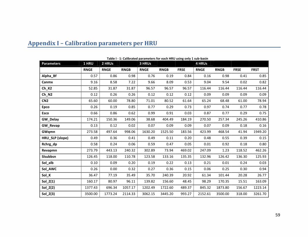
59

Appendix I – Calibration parameters per HRU

Table I - 1: Calibrated parameters for each HRU using only 1 sub-basin

Parameters 1 HRU 2 HRUs 3 HRUs 4 HRUs

RNGE RNGE RNGB RNGE RNGB FRSE RNGE RNGB FRSE FRST

Alpha_Bf 0.57 0.86 0.98 0.76 0.19 0.84 0.16 0.98 0.41 0.85

Canmx 9.16 8.58 7.22 9.66 8.09 0.53 9.04 9.54 0.02 0.82

Ch_K2 52.85 31.87 31.87 96.57 96.57 96.57 116.44 116.44 116.44 116.44

Ch_N2 0.12 0.26 0.26 0.12 0.12 0.12 0.09 0.09 0.09 0.09

CN2 65.60 60.00 78.80 71.01 80.52 61.64 65.24 68.48 61.00 78.94

Epco 0.26 0.19 0.85 0.77 0.29 0.73 0.97 0.74 0.77 0.78

Esco 0.66 0.86 0.62 0.99 0.91 0.03 0.87 0.77 0.29 0.75

GW_Delay 174.21 150.36 149.06 38.68 404.49 184.19 270.50 257.34 245.26 410.86

GW_Revap 0.13 0.12 0.02 0.07 0.09 0.09 0.07 0.09 0.18 0.16

GWqmn 273.58 497.64 998.06 1630.20 1525.50 183.56 423.99 468.54 41.94 1949.20

HRU_SLP (slope) 0.49 0.36 0.41 0.49 0.11 0.20 0.48 0.55 0.39 0.15

Rchrg_dp 0.58 0.24 0.06 0.59 0.47 0.05 0.01 0.92 0.18 0.80

Revapmn 273.79 443.13 240.32 302.89 73.94 469.02 247.09 1.23 118.52 462.26

Slsubbsn 126.45 118.00 110.78 123.58 133.16 135.35 132.96 126.42 136.30 125.93

Sol_alb 0.10 0.09 0.20 0.19 0.22 0.13 0.21 0.01 0.24 0.03

Sol_AWC 0.26 0.00 0.32 0.27 0.36 0.15 0.06 0.25 0.30 0.94

Sol_K 36.47 77.19 35.49 35.70 240.39 20.92 61.34 101.44 20.28 26.77

Sol_Z(1) 160.17 80.97 96.11 139.82 156.60 48.45 98.29 170.35 15.51 163.09

Sol_Z(2) 1377.43 696.34 1057.17 1202.49 1722.60 489.37 845.32 1873.80 156.67 1223.14

Sol_Z(3) 3500.00 1773.24 2114.33 3062.15 3445.20 993.27 2152.61 3500.00 318.00 3261.70