EVALUATION OF RANGE-WIDE OCCUPANCY AND SURVEY METHODS FOR

THE GIANT KANGAROO RAT (DIPODOMYS INGENS)

By

Alyssa Ellen Semerdjian

A Thesis Presented to

The Faculty of Humboldt State University

In Partial Fulfillment of the Requirements for the Degree

Master of Science in Natural Resources: Wildlife

Committee Membership

Dr. William “Tim” Bean, Committee Chair

Dr. Daniel Barton, Committee Member

Dr. Barbara Clucas, Committee Member

Dr. Andrew Stubblefield, Graduate Coordinator

May 2019

ii

ABSTRACT

EVALUATION OF RANGE-WIDE OCCUPANCY AND SURVEY METHODS FOR

THE GIANT KANGAROO RAT (DIPODOMYS INGENS)

Alyssa Ellen Semerdjian

Though habitat suitability and occupancy are often correlated, they cannot always

be inferred from each other. Therefore, a solid understanding of both is essential to

effectively manage species. Recent studies have assessed range-wide habitat suitability

for the giant kangaroo rat (Dipodomys ingens; GKR), but data regarding occupancy is

lacking in parts of its distribution. Satellite and aerial imagery were used to identify GKR

burrows across their known range, producing a range-wide occupancy map and non-

invasive survey methods including track plates, manned flight, unmanned aerial vehicle,

and sign surveys were conducted to determine effective methods for monitoring GKR

occupancy. The range-wide imagery survey detected well-studied GKR populations and

revealed populations in the center of its range where GKR occupancy was previously

unverified. Trapping results generally matched the range-wide imagery review findings

where GKRs were present, and these areas typically had high estimates of habitat

suitability. Manned flights accurately predicted GKR presence when compared to

available trapping data though the method did not match well with the range-wide

imagery survey. The sign surveys accurately predicted both GKR presence and absence

iii

according to the trapping data. The track plates only recorded partial kangaroo rat prints,

from which GKRs were indistinguishable from a sympatric species. Finally, the data

collected with the UAV was too limited to statistically assess, though anecdotally the

method shows promise as a GKR survey method. This study found that these techniques,

though informative on their own, are most effective when combined with at least one

other survey method to predict GKR presences. When used together, these non-invasive

practices will be an asset for conservationists interested in preserving habitat for GKRs.

iv

ACKNOWLEDGEMENTS

This project would not have been possible without the funding provided by the

California Department of Fish and Wildlife, the Bureau of Land Management, and the

Nature Conservancy, with guidance from Bob Stafford, Mike Westphal and Scott

Butterfield. Thank you for granting me the means to contribute to the conservation of

giant kangaroo rats and the San Joaquin Valley.

Thank you also to my advisor Tim Bean for giving me the chance to conduct this

research. I cannot express enough my appreciation for your patience and support. I also

want to thank every member of the Bean Lab who provided draft edits and study

suggestions, and my committee members Barbara Clucas and Dan Barton for their

contributions to my study design.

Many people contributed their time and energy to this project. I am exceedingly

grateful my field assistants Ian Axsom and Matilda Bunchonchitr who were enthusiastic

data collectors, even in tough conditions. I could not have done any of this without you.

Thank you also to the 33 volunteers that scoured through imagery looking for giant

kangaroo rat precincts, and especially to Abby Rutrough for helping me train volunteers

and compile the data.

As I wrap up this project I want to acknowledge those who have especially

contributed to the successes I have had so far. To my mom who taught me how to catch

lizards when I was a kid, to my dad who took me camping even though he hates sleeping

v

on the ground, and to my brothers, who tolerated hours of Animal Planet when they

would have rather been watching sports: thank you. You lead me down this path (much to

your bewilderment sometimes, I think) and gave me the freedom to follow it.

I am additionally indebted to my friends Ivy Widick, Jennie Jones-Scherbinski,

and Pairsa Belamaric for keeping me sane over the past three years. There is no one else I

would have rather experienced the highs and lows of graduate school with. And finally,

thank you to Tyler Summers, who learned, in rapid succession, of the existence of

kangaroo rats followed by an inane amount of facts about them as I worked on my

master’s degree. Thank you for steadfastly believing in me even at times when I didn’t

believe in myself. I am so grateful to you, and to everybody else that has supported me

through this project.

vi

TABLE OF CONTENTS

ABSTRACT II

ACKNOWLEDGEMENTS IV

TABLE OF CONTENTS VI

LIST OF TABLES VIII

LIST OF FIGURES X

LIST OF APPENDICES XI

INTRODUCTION 1

METHODS 11

Live Trapping 11

Range-Wide Imagery Survey 13

Manned Flight Surveys 17

UAV Surveys 17

Sign Surveys 18

Track Plates 20

RESULTS 22

Live Trapping 22

Range-Wide Imagery Survey 24

vii

Manned Flight Surveys 31

UAV Surveys 34

Sign Surveys 34

Track Plates 37

DISCUSSION 40

Live Trapping 40

Range-wide Imagery Survey 41

Manned Flight Surveys 47

UAV Surveys 48

Sign Surveys 49

Track Plates 52

CONCLUSIONS 54

LITERATURE CITED 57

APPENDICES 71

viii

LIST OF TABLES

Table 1: Outcomes for plots with 20 or fewer traps where at least 1 GKR was caught

from 2016 to 2017. 24

Table 2: Sensitivity, specificity and true skill statistics for the range-wide imagery survey,

using trapping data as the ‘truth’. Varying confidence scores were used as thresholds

to determine which range-wide imagery review cells would be compared to trapping

data. Confidence scores less than the threshold values were discarded for each test. 27

Table 3: Confusion matrix for live-trapping outcomes versus range-wide imagery review

findings. Matrix includes results for the 219 range-wide imagery survey cells

containing trapping sites and high confidence GKR presence-absence scores. GKRs

were considered ‘observed present’ when they were caught at least once on a plot

during trapping ‘observed absent’ when no GKRs were caught on a plot. GKRs were

‘predicted present’ when they were detected in the range-wide imagery review with a

confidence score greater than or equal to 3 and ‘predicted absent’ when observers

declared them absent with a confidence greater than or equal to 3. 28

Table 4: Confusion matrix for habitat suitability estimates vs. range-wide imagery review

findings. GKRs were considered ‘observed present’ when MaxEnt values were ≥ the

maximum sensitivity plus specificity threshold and ‘observed absent’ when they were

below the value. The maximum sensitivity plus specificity threshold was 0.19. GKRs

were ‘predicted present’ when they were detected in the range-wide imagery review

with a confidence score greater than or equal to 3 and ‘predicted absent’ when

observers declared them absent with a confidence greater than or equal to 3. 29

Table 5: Summary of trapping results for range-wide imagery review cells where GKR

were detected in the imagery and habitat suitability estimates were high, where they

were not detected in the imagery and habitat suitability estimates were high, where

they were detected in the imagery and habitat suitability estimates were low, and

where they were not detected in the imagery and habitat suitability estimates were

low. 31

Table 6: Average sensitivity, specificity and true skill statistics for boosted regression

trees built with data that was purposely altered to introduce false absences. The

sensitivity and specificity of ‘observed’ results, achieved using altered data are

compared to the sensitivity of the same models run using ‘actual’ or unaltered data.37

ix

Table 7: Sites with large kangaroo rat tracks registered on track plates and the GKR and

Heermann’s kangaroo rat capture rate at those sites. 38

Table 8: Individual track plates with large kangaroo rat tracks and the capture rate of

GKR and Heermann’s kangaroo rats at the traps set next to each track plate. 39

x

LIST OF FIGURES

Figure 1: Historical GKR range outlined in black (Williams 1992), areas referenced

frequently in this study are outlined with angled line fill and have corresponding

labels. Public lands in shown with vertical lines (CPAD 2017). Agriculture and urban

development as of 2011 is shown in light gray (Homer et al. 2015), and oil and gas

extraction sites that are active or in the process of being built as of June 2018 are in

dark gray (CDOGGR 2016). 9

Figure 2: NAIP images of A) sparse GKR precincts, B) small mammal sign, not GKRs

C) cattle sign, D) mima mounds E) Dense GKR colony 14

Figure 3: Track plate construction with: a) assembly of bait, blotter paper, and felt ink

pads on the plastic base b) configuration of blotter paper and felt ink pads when

attached to bottom gutter segment c) finished track tube with bolts and eye bolts

attaching the top and bottom gutter segments. 21

Figure 4: Sites trapped between 2010 and 2017. White dots symbolize sites where no

GKRs were caught; black dots symbolize sites where they were captured. Gray

shaded areas represent key GKR populations (Panoche, Carrizo, and Lokern) and

other locations of particular interest for this study (Kettleman Hills and Wind Wolves

Preserve). 23

Figure 5: Historical GKR species distribution in black and average observer confidence

on the presence or absence of GKRs. Black indicates high confidence that GKRs

were present, light gray indicates high certainty that GKRs were absent, shades in

between represent presence or absence with less certainty. 25

Figure 6: Historically suitable habitat as determined by a MaxEnt model thresholded to

the maximum sensitivity plus specificity (Rutrough et al. revised review) in angled

lines, locations where GKRs were observed during manned flight surveys in light

gray, range-wide imagery review cells where GKRs were observed with a confidence

of three or higher in dark gray, and sites where GKRs were trapped in black. 33

Figure 7: Relative influence for all variables used in boosted regression trees comparing

sign surveys to live trapping. 35

Figure 8: Relative influence for all variables used in boosted regression trees comparing

sign surveys to range-wide imagery review results. 36

xi

LIST OF APPENDICES

Appendix A: Sign categories recorded during non-invasive GKR surveys. 71

Appendix B: Track plate design protocol 73

Appendix C: Boosted regression tree model selection, sorted by deviance 74

1

INTRODUCTION

Effective conservation plans rely on a thorough understanding of habitat

suitability and occupancy for target species. Habitat suitability, or the extent to which the

elements necessary to promote the growth and stability of populations for a species are

available in a given area (Kellner et al. 1992), and occupancy - whether or not a species is

present at a location - are conceptually linked (Pulliam 2000). However, while the two

are often positively correlated, occupancy and habitat suitability cannot always be neatly

inferred from each other. Populations may occur in areas with low suitability.

Fragmentation, modification, and abrupt changes in climate or other environmental

conditions can leave remnant populations in habitat that lacks the resources to optimally

sustain them (Clevenger et al. 1997, Schlaepfer et al. 2002), and sink populations can

persist in unsuitable locations as long as they are replenished by a source population

(Pulliam 1988). Conversely, the stochastic processes of population dynamics may result

in suitable areas not being occupied continuously (Eriksson 1996).

Because the relationship between habitat suitability and occupancy is imperfect, it

is important to assess both for species in need of protection (Pulliam 2000). Modeled

estimates of habitat suitability are useful for identifying potential protected areas as well

as connectivity corridors. However, the actions taken to protect areas highlighted by

suitability models depend largely on whether species of concern are present. Areas that

are occupied by sensitive species are often given the highest priority in conservation

plans (USFWS 1998, Fox & Nino-Murcia 2005), especially if those areas have high

2

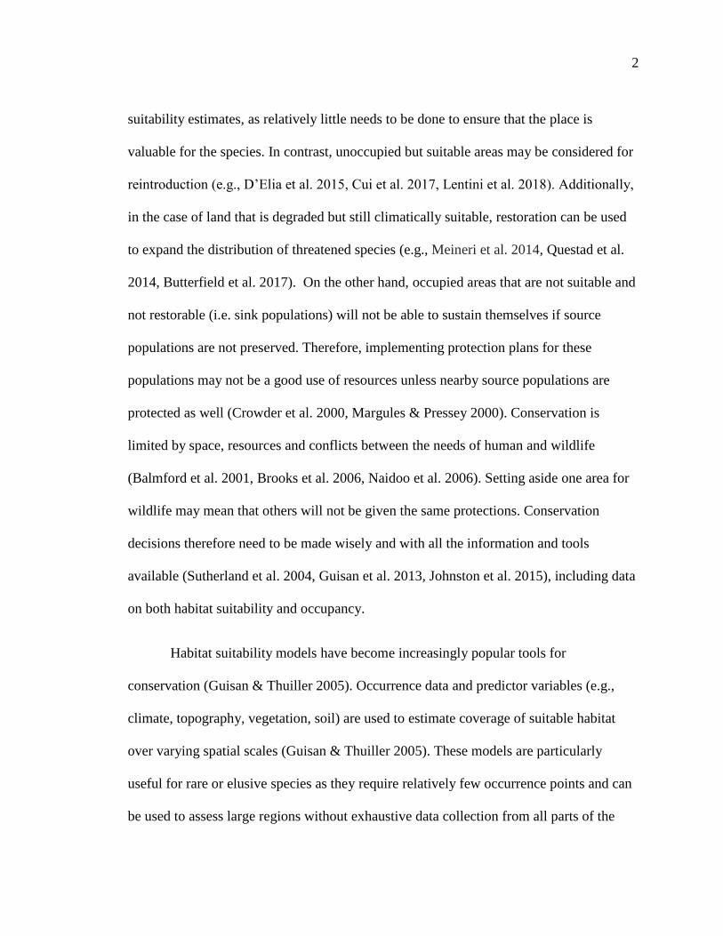
suitability estimates, as relatively little needs to be done to ensure that the place is

valuable for the species. In contrast, unoccupied but suitable areas may be considered for

reintroduction (e.g., D’Elia et al. 2015, Cui et al. 2017, Lentini et al. 2018). Additionally,

in the case of land that is degraded but still climatically suitable, restoration can be used

to expand the distribution of threatened species (e.g., Meineri et al. 2014, Questad et al.

2014, Butterfield et al. 2017). On the other hand, occupied areas that are not suitable and

not restorable (i.e. sink populations) will not be able to sustain themselves if source

populations are not preserved. Therefore, implementing protection plans for these

populations may not be a good use of resources unless nearby source populations are

protected as well (Crowder et al. 2000, Margules & Pressey 2000). Conservation is

limited by space, resources and conflicts between the needs of human and wildlife

(Balmford et al. 2001, Brooks et al. 2006, Naidoo et al. 2006). Setting aside one area for

wildlife may mean that others will not be given the same protections. Conservation

decisions therefore need to be made wisely and with all the information and tools

available (Sutherland et al. 2004, Guisan et al. 2013, Johnston et al. 2015), including data

on both habitat suitability and occupancy.

Habitat suitability models have become increasingly popular tools for

conservation (Guisan & Thuiller 2005). Occurrence data and predictor variables (e.g.,

climate, topography, vegetation, soil) are used to estimate coverage of suitable habitat

over varying spatial scales (Guisan & Thuiller 2005). These models are particularly

useful for rare or elusive species as they require relatively few occurrence points and can

be used to assess large regions without exhaustive data collection from all parts of the

3

study area (Stockwell & Peterson 2002). The models can also be projected using

estimates of future or past climate conditions to extrapolate habitat suitability estimates in

different time periods (Araújo et al. 2005). These projections are especially useful in a

conservation context, as they can identify areas that may be suitable for sensitive species

in the future, and therefore, with careful consideration, can be used to inform predictive

management plans (Hijmans & Graham 2006).

Though habitat suitability models are informative, they are not without critics.

There are a number of reasons why these models may not capture true underlying

suitability. Models outputs are partly dependent on inputs chosen by a researcher and the

results can be affected by the methods and predictors that are selected (Guisan &

Zimmerman 2000, Wilson et al. 2005). Inaccurate models can result from a number of

errors, including the use predictor data that is inaccurate, incomplete, or of unsuitable

spatial resolution (Guisan & Zimmerman 2000, Araújo & Peterson 2012). In addition to

issues with environmental predictors, species occurrence data can also negatively affect

the accuracy of the model if they are spatially biased (Bean et al. 2012a). If the

occurrence data that is used to build models does not include detections across the

complete range of conditions that the species can tolerate then the resulting habitat

suitability estimates will not include the entirety of the species’ fundamental niche

(Hutchinson 1957). Limited dispersal ability (Pearson & Dawson 2003), exclusion from

otherwise suitable habitat by anthropogenic or other biotic means (Scheele et al. 2017),

and short-term changes in occupancy (Bean et al. 2012a), for example, can affect the data

used to build habitat suitability models, which can change the outcome of those

4

predictions. Even if these errors are avoided, a well-designed habitat suitability model

will highlight areas with the right conditions to support healthy populations, but they do

not necessarily reflect the reality of where the species actually occurs, especially if

populations are not at equilibrium with the environment (Araújo & Peterson 2012).

Because of these issues, managers should supplement habitat suitability estimates with

up-to-date occupancy data before making decisions.

There are many ways to monitor species occupancy across a landscape. Live

trapping is considered to be one of the most effective means of gathering information,

including occupancy status, for many species, especially small mammals (Glennon et al.

2002). A benefit of live trapping is that a variety of data can be collected from each

captured animal that can be used to answer a multitude of questions beyond occupancy.

However, live trapping can be time intensive and expensive. It can also cause damage to

habitat due to trampling from frequent site visits, and can stress captured animals while

putting them at risk of injury or death (Glennon et al. 2002). Less invasive tactics such as

camera trapping, hair snares, transect sign surveys, and track plates cause far less stress to

the study animals, though they are often less informative (Van Horne et al. 1997). Under

certain conditions, however, data collected from these methods can be used as indices to

effectively monitor populations (Hubbs et al. 2000, Stanley & Royle 2005). Methods that

collect or record sign (i.e. hair snares, track plates and camera trapping) can be expensive

depending on the materials needed, and still require occasional site visits from

technicians. However, equipment can usually be left unchecked for longer periods of

time, resulting in less human disturbance and a wider temporal window for animal

5

detections (Gompper et al. 2006). Depending on the study design, transect sign surveys

can require even fewer site visits. Some species can have a higher probability of detection

over a shorter amount of time in sign surveys than cameras or track plates (Gompper et

al. 2006).

Aerial surveys are another potential method for detecting species that are large

(Smyser et al. 2016, Greene et al. 2017), live in dense colonies (Hodgson et al. 2015), or

create especially visible sign (Puttock et al. 2015). Unmanned aerial vehicles (hereafter:

UAVs) (Vermeulen et al. 2013, Weissensteiner et al. 2015), manned flight surveys

(Smyser et al. 2016) and satellites (Rocchini et al. 2015) have all been used to assess

species presence and abundance over large regions. Each of these techniques differs in

costs and quality of information depending on the methods and type of equipment used.

UAVs have the potential to provide data with high spatial accuracy and temporal

precision (Hodgeson et al 2015), though they cannot survey as large an area as the other

aerial methods in a given amount of time. Manned aircraft can be used to survey broader

regions than UAVs in the same amount of time while providing temporally precise data.

However, manned flight surveys can be expensive and impose some risk for the pilot and

observers. Satellite and high altitude flight imagery can be used to survey very broad

areas compared to the other two methods, though depending on the data source, the

temporal precision and spatial accuracy could be much lower. Aerial surveys are limited

not only by data quality, cost, and time, but also by the fact that they can only be used for

species or sign that are visible from the air (Greene et al. 2017).

6

The giant kangaroo rat (Dipodomys ingens, hereafter, GKR) is an endangered

rodent uniquely suited to aerial monitoring. The GKR is endemic to California’s San

Joaquin Valley where individuals defend territories within colonies. They build elaborate

burrow structures, called precincts, which provide thermal refuges that are vital to their

survival (Grinnell 1932, Kay & Whitford 1978). GKRs also use their precincts to store

seeds, which they gather and place in shallow pit caches on the surface of their precincts

and in deep caches within their burrows (Shaw 1934). Burrows and their associated food

stores are fiercely defended against conspecific and heterospecific intruders by a single

GKR, or by a mother and her offspring prior to their dispersal (Jones 1993, Cooper &

Randall 2007). When a kangaroo rat dies or disperses its burrow is often taken over by

another, resulting in continuous occupation (Grinnell 1932, Schooley & Wiens 2001).

Sustained burrowing activity over many generations leads to the accumulation of

soil around burrows, forming precincts into mounds (Best 1972). GKR mounds are

typically positioned about 20 meters apart from each other, center to center, creating a

visible pattern on the landscape and signaling the amount of territory that GKRs are able

to defend from encroaching neighbors (Grinnell 1932, Braun 1985, Cooper & Randall

2007). In addition to observable topographic patterns, the interaction between GKRs and

vegetation make active precincts obvious landscape features (Grinnell 1932, Prugh et al.

2012). GKRs clip the vegetation so that by late spring there are clear bare patches

covering their burrows, which contrast with the vegetated areas in between territories.

Precincts are also distinctive during the rainy season and into early spring when the seeds

gathered by GKRs germinate and grow in patches that are thicker than the surrounding

7

vegetation. Though these features are most obvious when precincts are active, GKRs

produce lasting topographic and vegetation legacies (Grinath et al. 2017) that can be seen

for up to a decade after GKR extirpation (J. Chestnut, personal communication, 30

August 2018).

Though conspicuous on the landscape, GKR occupancy throughout their range

can be difficult to establish due to their historically patchy distribution (Grinnell 1932).

This problem has been further exacerbated in the past century by habitat fragmentation

primary driven by agricultural development (Williams 1992). Though habitat suitability

estimates have been thoroughly assessed in recent years (Bean et al. 2014b, Widick 2018,

Widick & Bean 2019, Rutrough et al. revised review) there are significant gaps in

observed occupancy data. GKRs are limited by very specific habitat needs. They avoid

thick vegetation and sloped terrain and tend to live in the wettest parts of the arid San

Joaquin Valley (Bean et al. 2014b). Their small range combined with the visible sign they

create provides a unique opportunity to conduct a range-wide occupancy survey.

Although an assortment of public and private agencies regularly survey for GKRs on

their properties, there has not been a recent range-wide assessment of their distribution

(USFWS 2010). A quick and reproducible method for assessing occupancy would help

managers monitor GKR distribution and track changes from year to year, which is

especially important because GKR populations fluctuate extensively with drought cycles

(Prugh et al. 2018). In addition to the need for range-wide monitoring, there are currently

no standardized field protocols for non-invasive methods to monitor GKRs. Tested,

8

standardized, non-invasive detection methods for GKRs would help different agencies

charged with monitoring GKRs compare data, and could be used alone or in coordination

with remote surveys.

This study sought to determine GKR occupancy throughout their range while testing

the efficacy of non-invasive survey methods including 1) the review of high altitude

imagery, 2) manned flight, 3) UAV, and 4) on-the-ground sign surveys, and 5) track

plates. Each of these methods were tested against trapping data in order to calculate

perceived proportions of correctly classified presence and absence determinations for

each type of survey, and the high-altitude imagery survey was also compared to habitat

suitability estimates.

I expected to easily detect GKR sign in areas where GKRs are already known to be

located in the range-wide imagery survey, especially in the Carrizo Plain National

Monument (hereafter: Carrizo), Ciervo-Panoche Natural Area (hereafter: Panoche) and

Lokern (Figure 1). I also expected to detect them in less understood areas in the center of

their range, particularly around the Kettleman Hills area (Figure 1). I expected a low rate

of false absences from this survey method because GKR sign is distinct and easily

recognizable, however, I expected there to be a higher rate of false presences because

some sign, such as GKR mounds can persist on the landscape for years after extirpation

and at very high altitudes the age of sign is indeterminable. When comparing the range-

wide imagery survey to habitat suitability estimates, I expected most occupied areas to

have high habitat suitability estimates, though I anticipated that there would be more land

9

that is estimated to climatically suitable than is occupied, primarily due to the amount of

land converted for human use in the GKR historical range.

Figure 1: Historical GKR range outlined in black (Williams 1992), areas referenced

frequently in this study are outlined with angled line fill and have corresponding

labels. Public lands in shown with vertical lines (CPAD 2017). Agriculture and

urban development as of 2011 is shown in light gray (Homer et al. 2015), and oil

and gas extraction sites that are active or in the process of being built as of June

2018 are in dark gray (CDOGGR 2016).

10

The UAV and manned flight surveys both rely on recent GKR sign such as vegetation

clipping to determine the location of active precinct, therefore I expected these methods

to be more accurate than the range-wide imagery review. While I expected the results of

the flight and UAV methods to be similar, I predicted that imprecision stemming from

conducting surveys at a higher altitude, as well as the observer error introduced by

collecting data in real time versus reviewing high quality images gathered from the field,

would cause the manned flight results to differ more from trapping data then the UAV

surveys (Bean et al. 2012b). GKRs create unique and plentiful sign on their precincts and

are active and easily baited during the summer, so the transect sign surveys and track

plates were expected to be closely correlated with occupancy at the site level.

By comparing the results of the range-wide imagery surveys to previous GKR habitat

suitability models, this study aimed to provide insight into where GKRs are currently

found and where they potentially could be. The range-wide imagery survey was also

assessed as one of several non-invasive field methods for assessing occupancy

throughout the GKR range. These findings will inform management decisions and

provide standardized methods for collecting GKR data in the future.

11

METHODS

The overall goals of this project were to produce a map of range-wide occupancy for

GKRs generated by a systematic review of aerial and satellite imagery, and to test a

number of non-invasive techniques for estimating GKR occupancy at varying spatial

levels. Live trapping is considered the ‘gold standard’ for monitoring GKRs (Bean et al.

2012b). Therefore, the results of the track plates, imagery review, manned flights, UAV,

and sign surveys were tested against trapping data. The range-wide imagery review was

also compared to a MaxEnt model from a recent study (Rutrough et al. revised review) to

assess the relationship between habitat suitability estimates and occupancy throughout the

GKR range.

Live Trapping

GKR live trapping was conducted between 2010 and 2017. The majority of

trapping occurred in the Carrizo and the Panoche, though some trapping took place in the

center of the range and in areas adjacent to the Carrizo in 2017 (Bean et al. 2014a,

Alexander 2016, Widick 2018, Widick & Bean 2019). Sherman XL live traps were baited

with millet-based birdseed and checked for 3 to 5 nights per session during summer

months. Captured animals were identified to species and either given individually

numbered ear tags or temporary marks with permanent markers. Trapping followed

American Society of Mammalogists guidelines (Sikes et al. 2011) and was conducted

under US Fish and Wildlife permits TE37418A-3. Scientific Collecting Permit SC-

12

11135, Humboldt State Animal Care Protocol 13-14.W.109-A and 16/17.W.96-A, and an

MOU from California Department of Fish & Wildlife.

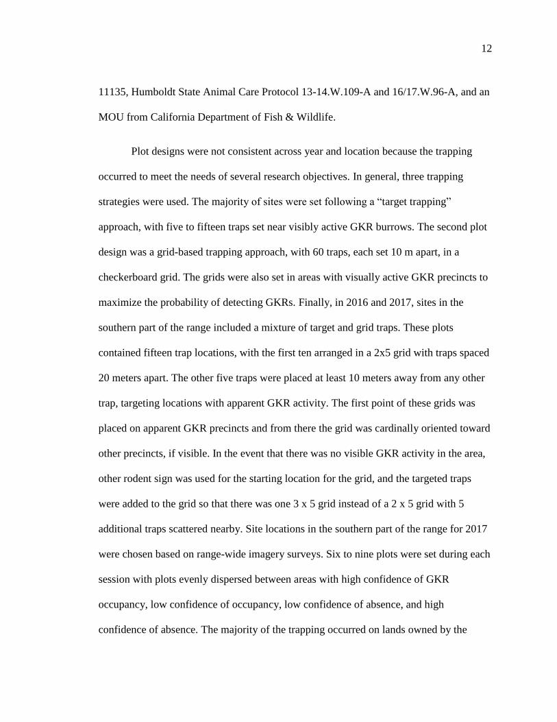
Plot designs were not consistent across year and location because the trapping

occurred to meet the needs of several research objectives. In general, three trapping

strategies were used. The majority of sites were set following a “target trapping”

approach, with five to fifteen traps set near visibly active GKR burrows. The second plot

design was a grid-based trapping approach, with 60 traps, each set 10 m apart, in a

checkerboard grid. The grids were also set in areas with visually active GKR precincts to

maximize the probability of detecting GKRs. Finally, in 2016 and 2017, sites in the

southern part of the range included a mixture of target and grid traps. These plots

contained fifteen trap locations, with the first ten arranged in a 2x5 grid with traps spaced

20 meters apart. The other five traps were placed at least 10 meters away from any other

trap, targeting locations with apparent GKR activity. The first point of these grids was

placed on apparent GKR precincts and from there the grid was cardinally oriented toward

other precincts, if visible. In the event that there was no visible GKR activity in the area,

other rodent sign was used for the starting location for the grid, and the targeted traps

were added to the grid so that there was one 3 x 5 grid instead of a 2 x 5 grid with 5

additional traps scattered nearby. Site locations in the southern part of the range for 2017

were chosen based on range-wide imagery surveys. Six to nine plots were set during each

session with plots evenly dispersed between areas with high confidence of GKR

occupancy, low confidence of occupancy, low confidence of absence, and high

confidence of absence. The majority of the trapping occurred on lands owned by the

13

Bureau of Land Management, though California Department of Fish and Wildlife, United

States Fish and Wildlife Service, Wildlands Conservancy, and private lands were also

accessed with permission.

Range-Wide Imagery Survey

Satellite and aerial imagery were used to identify areas with visible GKR sign to

create a range-wide occupancy map. A set of 5 km2 grids and 1 km2 cells were

superimposed over a 10 km buffer around the historical GKR range map (Williams 1992)

(Figure 1) so that twenty-five 1 km2 cells fit inside each 5 km2 grid. Imagery within all 5

km cells contained in, or touching the buffer, was surveyed.

A team of 33 undergraduate volunteers and 3 project coordinators assisted in the

survey. Each observer attended a training session where they were shown examples of

aerial images of verified GKR burrows (Figure 2), as well as comparison images of other

visually similar landscape features that might be confused with GKR precincts, such as

other small mammal burrows, cattle sign, and dome-shaped topographic features called

mima mounds (Figure 2). Project coordinators monitored observer performance until

their findings consistently matched the coordinators, and then volunteers were able to

work on their own.

14

Figure 2: NAIP images of A) sparse GKR precincts, B) small mammal sign, not GKRs

C) cattle sign, D) mima mounds E) Dense GKR colony

The survey utilized the default ArcMap basemap imagery which consisted of

high-resolution National Agriculture Imagery Program (NAIP) images from 2014 and

lower resolution Satellite Pour l'Observation de la Terre (SPOT) from 2008. Observers

surveyed one 5 km2 grid at a time. They zoomed to each 1 km2 cell within the grid and

searched using map ratios between 1:5,000 and 1:1,000. After scrolling through the entire

1 km2 unit they noted whether GKRs were present in that cell and marked their

confidence in their decision on a scale from 1 to 5. Presence designation and confidence

in presence decisions were consolidated into a single score. Cells where observers

indicated that GKRs were present were given positive values and cells where no GKRs

were found were given negative value, so that a score of 5 indicated that the observer

found GKRs in the cell and were very confident of their findings, a score of -5 indicated

that the observer was very confident that there were no GKRs in the cell, and scores in

between indicated GKR presence or absence with less certainty.

15

Two observers assessed each cell and the scores were averaged, except in the case

of disagreement about GKR occupancy. In these instances, a project coordinator also

surveyed the cell. The confidence scores for coordinator and the volunteer that agreed on

GKR occupancy were averaged. Averaged scores were compiled to create a map

indicating areas where GKRs were present or absent, and the confidence level of each

observation. The results of the range-wide imagery review were tested against trapping

data collected between 2010 and 2017. In several cases, there were multiple trapping sites

within a single 1 km2 range-wide imagery survey cell. GKRs only had to be captured at

one site within a cell to consider GKRs ‘captured’ in that unit.

The range-wide imagery survey was tested against trapping data using different

confidence scores to determine whether GKRs were ‘present’ or ‘absent’ in a cell. In

separate tests, trapping data was compared to range-wide imagery cells with confidence

scores greater than or equal to 1, 2, 3, or 4, or equal to 5. The proportion of cells that

correctly identified GKR presence (sensitivity) and the number of cells correctly

identified GKR absence (specificity) were calculated using trapping results and the

presence-absence findings for each confidence category from the range-wide review.

The relationship between range-wide GKR occupancy and habitat suitability

estimates was also assessed. A recent study reconstructed the historical distribution of

GKRs using precincts detected in aerial imagery dating before 1960 as presence points to

create a MaxEnt model for their historical range (Rutrough et al. revised review).

Climatic water deficit, or the quantification of how local conditions supporting

16

evaporation exceed the amount of water available for actual evaporation (Stephenson

1998), slope, and soil qualities were the predictors in their top model. This model was

projected using modern climatic values to estimate current suitability for GKRs across

their range (Rutrough et al. revised review). Values from the modern projection of the

MaxEnt model were extracted at the center of each 1 km2 range-wide imagery survey

cell. The model pixels were 0.810 km by 0.810 km. Because they were slightly smaller

than the range-wide imagery survey cells, no single MaxEnt pixel was extracted from the

center of a range-wide imagery review cell more than once. For the purpose of this

analysis GKRs were considered ‘present’ when MaxEnt values were greater than or equal

to the maximum sensitivity plus specificity threshold (Bean et al 2012a), and were

considered ‘absent’ when the value was less. The maximum sensitivity plus specificity

threshold, and resulting sensitivity and specificity for the habitat-range-wide imagery

review test were calculated using the R package PresenceAbsence (R core team 2018,

Freeman & Moisen 2008). Additionally, the trapping results for range-wide imagery

review cells that contained trapping sites and had confidence values above three were

summarized based on whether the cell was in suitable habitat and GKR were detected in

the imagery, unsuitable habitat and GKR were detected in the imagery, suitable habitat

with no GKR detections in the imagery, and unsuitable habitat with no GKR detected in

the imagery.

17

Manned Flight Surveys

California Department of Fish and Wildlife conducted flight surveys for GKRs in

the summer and fall of 2011, 2016 and 2017. A pilot followed pre-designed transects

while two observers watched the landscape, one on each side of the plane, and recording

GPS tracks when they saw GKR sign. Buffers were created post-hoc to fit in the space

tracks signifying GKR sign to approximate observer line of site. In 2011 the buffers were

750m on each side of the flight lines and in 2016 and 2017 the buffers were 600m on

each side. Positive predictive values for the flight data were calculated using trapping

and, separately, range-wide imagery review results set to binary presence or absence

values. Cells where GKR were present were those where sign was detected with a

confidence score of three or higher. GKR were considered absent in cells where sign was

not detected with a confidence of three or higher. Sensitivity, specificity and negative

predictive values could not be calculated because the total area flown, and therefore

places where GKRs were absent in the flights, was not available.

UAV Surveys

A DJI Phantom 3 Standard UAV equipped with a camera and GPS was used to

help locate GKR precincts and determine trapping and survey locations during the

summer of 2017. The UAV was controlled through either the DJI GO (SZ DJI

Technology Co. Ltd 2018) or Litchi (VC Technology Ltd 2018) application on an iPhone

6s. Observers searched for GKR activity in video live-feed recorded between 30 to 400

18

feet above the ground around potential trapping sites. These flights were not systematic;

rather they were intended to assist in fine-scale trapping site selection.

The UAV was also used to conduct standardized GKR surveys using pre-

programmed missions and user defined waypoints in the Litchi app. Photos were taken

every 100 meters with the camera angled straight down during the course of a 500-meter

by 100-meter rectangular flight path. I assessed whether GKR sign was present in the

photos using the same system as the range-wide imagery surveys.

Sign Surveys

This study sought to develop a standardized, non-invasive on-the-ground sign

survey to determine GKR occupancy as a potential replacement for live trapping. Data

were collected in the southern part of the GKR range in 2016 and 2017 and in the

Panoche and surrounding area in 2017. Observers were trained by conducting surveys

together on several plots and comparing results at the end of each survey until new

observers consistently had results similar to more experienced data collectors. After

training was completed, typically two observers started at opposite ends of a plot and

worked toward each other until all survey locations had been visited.

The sign surveys were conducted once on each trapping plot during the session in

which it was trapped. Survey points coincided with trap locations. The survey involved

recording the presence of designated types of sign within a meter radius of each point.

The sign categories included variables that were thought to correlate with GKR presence,

19

such as tracks and scats as well as variables that might indicate a lack of recent activity or

burrow maintenance suggesting GKR absence, such as spider webs or debris in burrow

openings (Appendix A). The survey was designed to be non-subjective by requiring only

binary determinations of whether each sign category is present or absent, with no further

quantifications. Additionally, the protocol was intended to be simple so that observers

could collect data regardless of their level of prior GKR monitoring experience.

The proportion of trap locations where each sign category was observed was

calculated for each plot. These proportions were used to test whether the surveys could

predict GKR occupancy using boosted regression trees in the R package ‘gmb’

(Greenwell et al. 2018). Separate models were built using occupancy as determined by

trapping data and the range-wide imagery review. The trapping models included data

from 163 sites surveyed and trapped in 2016 and 2017. The range-wide imagery review

models only used presence and absence data from survey cells with confidence scores

greater than or equal to three. Cells with lower scores were removed from the analysis.

The 85 sign survey sites that fell within cells with compatible range-wide imagery review

scores were analyzed. Sensitivity and specificity for the models with the lowest deviance

were calculated using five-fold cross validation.

Though trapping is considered an accurate method for determining GKR

presence, it is possible that GKR were not caught at all sites where they were present. To

test how sensitive the boosted regression tree analysis was to false negatives, datasets

were created with known amounts of false negatives added in. In separate analyses

20

boosted regression trees were run on data with 5%, 10%, 25% and 50% of the sites where

GKR were captured altered to falsely indicate that no GKR were caught there. Ten

datasets with randomly selected false negatives were built for each percentage category.

Top models for the forty datasets were chosen from the same candidate model set used to

initially analyze the sign surveys (Appendix C). The top model for each data set was the

one with the lowest deviance. Sensitivity, specificity, and true skill statistics were

calculated for each top model using five-fold cross validation. Each top model was run

again using unaltered, and specificity, sensitivity and true skill statistics were similarly

calculated for each using five-fold cross validation.

The sensitivity, specificity and true skill statistics for the ten models built using

data with each percentage of known false negatives were averaged, as were the

corresponding values from the associated models run using unaltered data. The averaged

sensitivities, specificities, and true skill statistics were compared to assess whether the

results of boosted regression trees run with data with known false absences differ from

models with no verified false absences.

Track Plates

Track plates were deployed as another non-invasive survey method in the

southern part of the GKR range during the summer of 2017 (Appendix B, Figure 3. Track

plates were placed alongside traps, alternating between targeted and grid traps. Five track

plates were deployed at each site where they were used. The blotter paper would be

21

removed from the plastic backing upon collection. If there were tracks, the blotter paper

would be sprayed with an art fixative and stored until the tracks could be identified.

Tracks present on each card were identified to species, when possible, using the Peterson

Field Guide to Animal Tracks (Murie & Elbroch 2005) with the aid of previous

knowledge of the species found in the trapping areas. Sensitivity and specificity were

calculated to test the track plates’ ability to detect kangaroo rats against live trapping.

Figure 3: Track plate construction with: a) assembly of bait, blotter paper, and felt ink

pads on the plastic base b) configuration of blotter paper and felt ink pads when

attached to bottom gutter segment c) finished track tube with bolts and eye bolts

attaching the top and bottom gutter segments.

22

RESULTS

Live Trapping

GKR were successfully captured at 289 of 436 trapping sites set across 5 counties

in central California from 2010 to 2017 (Figure 4). GKRs were caught at 86 of the 148

plots trapped in and around the Carrizo in San Luis Obispo and Kern Counties, CA, 190

of the 279 plots in and around the Panoche in Fresno and San Benito Counties, CA and 3

of the 9 plots in the Kettleman Hills in Kings County, CA. During eight years that

trapping occurred, 1,581 individual GKRs were captured and tagged. For plots where at

least one GKR was caught, overall trap success was typically lowest on the first night of

each session and highest on the fifth, though most plots were only trapped for three nights

(Table 1). Conversely, the highest proportion of first GKR captures per site occurred on

the first night of trapping, tapering considerably by the fifth night (Table 1).

23

Figure 4: Sites trapped between 2010 and 2017. White dots symbolize sites where no

GKRs were caught; black dots symbolize sites where they were captured. Gray

shaded areas represent key GKR populations (Panoche, Carrizo, and Lokern) and

other locations of particular interest for this study (Kettleman Hills and Wind

Wolves Preserve).

24

Table 1: Outcomes for plots with 20 or fewer traps where at least 1 GKR was caught

from 2016 to 2017.

Night of session (n =

number of plots)

Proportion of traps

that captured GKRs

on the plot per

session

Proportion of plots

that caught their first

GKR on a given

night

Night 1 (n=138) 0.059 0.464

Night 2 (n=137) 0.139 0.341

Night 3 (n=129) 0.193 0.145

Night 4 (n=94) 0.184 0.044

Night 5 (n=43) 0.225 0.007

Range-Wide Imagery Survey

In total, observers reviewed imagery covering 17,375 km2 of the San Joaquin

Valley for GKR sign. Scores denoting observer confidence in GKR presence or for each

1 km2 cell were compiled to create a range-wide map of GKR detections (Figure 5).

GKRs were absent with a confidence score greater than or equal to 3 in 89.4% of the

cells, GKR occupancy was uncertain in 4.5%, and GKRs were determined to be present

with a confidence score of 3 or higher in 6.1% of the cells searched. Out of the 17,375

cells surveyed, 5,718 intersected or were contained within public or protected land. GKR

25

were observed with a confidence of 3 or higher in 9.8% of the cells intersecting public

lands. Occupancy was uncertain in 5.5%, and GKRs were determined absent in 84.7% of

those cells.

Figure 5: Historical GKR species distribution in black and average observer confidence

on the presence or absence of GKRs. Black indicates high confidence that GKRs

were present, light gray indicates high certainty that GKRs were absent, shades in

between represent presence or absence with less certainty.

26

Trapping data collected between 2010 and 2017 were used to assess the accuracy

of the range-wide imagery survey. There were 256 range-wide imagery review cells that

contained trapping sites16 had a confidence score of one, 21 had a confidence score of

two, 57 had a confidence score of three, 81 had a confidence score of four, and 81 had a

confidence score of five. Sensitivity and specificity were lowest when all confidence

values were included (Table 2). Both sensitivity and specificity increased as confidence

scores increased, except that specificity dropped when only cells with confidence scores

of five were used (Table 2).

27

Table 2: Sensitivity, specificity and true skill statistics for the range-wide imagery survey,

using trapping data as the ‘truth’. Varying confidence scores were used as

thresholds to determine which range-wide imagery review cells would be

compared to trapping data. Confidence scores less than the threshold values were

discarded for each test.

#

cells

Sensitivity

Sensitivity

standard

deviation

Specificity

Specificity

standard

deviation

True

skill

statistic

Confidence ≥ 1 256 0.768 0.040 0.465 0.0417 0.233

Confidence ≥ 2 240 0.784 0.041 0.457 0.0426 0.241

Confidence ≥ 3 219 0.809 0.0419 0.469 0.044 0.278

Confidence ≥ 4 162 0.841 0.0464 0.515 0.050 0.356

Confidence ≥ 5 81 0.880 0.066 0.393 0.066 0.273

Cells with a confidence level of three or higher were used for further analysis in

this study. This confidence score was chosen because sensitivity and specificity were

fairly high, and including some cells with confidence scores lower than 4 would include

areas where observers were reasonably certain that GKR were present that may be of

28

interest to managers and should be subject to further investigation. There were 219 range-

wide imagery survey cells that contained trapping sites and had confidence scores of

three or higher and GKRs were caught in 141 of them. GKRs were caught in 64 of the

107 cells in and around the Panoche, 74 of the 103 cells in and around the Carrizo, and 3

of the 9 cells in Kettleman Hills. GKRs were successfully trapped at most of the sites that

were located in cells where they were detected in the range-wide imagery review

(sensitivity = 0.809, SD = 0.042), however, they were also captured in about half of the

trapped cells where they were thought to be absent based the range-wide review

(specificity = 0.479, SD = 0.044) (Table 3). The true skill statistic for this test was 0.278

(Allouche et al. 2006).

Table 3: Confusion matrix for live-trapping outcomes versus range-wide imagery review

findings. Matrix includes results for the 219 range-wide imagery survey cells

containing trapping sites and high confidence GKR presence-absence scores.

GKRs were considered ‘observed present’ when they were caught at least once on

a plot during trapping ‘observed absent’ when no GKRs were caught on a plot.

GKRs were ‘predicted present’ when they were detected in the range-wide

imagery review with a confidence score greater than or equal to 3 and ‘predicted

absent’ when observers declared them absent with a confidence greater than or

equal to 3.

Present in range-wide imagery

review

Absent in range-wide imagery

review

GKR trapped 72 69

No GKR trapped 17 61

29

Range-wide imagery survey results were compared to MaxEnt values to

determine whether occupancy could be predicted from habitat suitability estimates. The

maximum sensitivity plus specificity threshold used for the MaxEnt values was 0.190.

There were very few instances where GKRs were detected in the range-wide imagery

review in areas with habitat suitability estimates below the threshold (specificity =

0.989), however, there were many areas where habitat suitability estimates exceeded the

threshold but GKR sign was not detected in the range-wide imagery review (sensitivity =

0.114) (Table 4). The true skill statistic for this test was 0.103 (Allouche et al. 2006).

Table 4: Confusion matrix for habitat suitability estimates vs. range-wide imagery review

findings. GKRs were considered ‘observed present’ when MaxEnt values were ≥

the maximum sensitivity plus specificity threshold and ‘observed absent’ when

they were below the value. The maximum sensitivity plus specificity threshold

was 0.19. GKRs were ‘predicted present’ when they were detected in the range-

wide imagery review with a confidence score greater than or equal to 3 and

‘predicted absent’ when observers declared them absent with a confidence greater

than or equal to 3.

Habitat suitability estimate

above threshold

Habitat suitability estimate

below threshold

Present in range-wide

imagery review 968 88

Absent in range-wide

imagery review 7,528 7,914

30

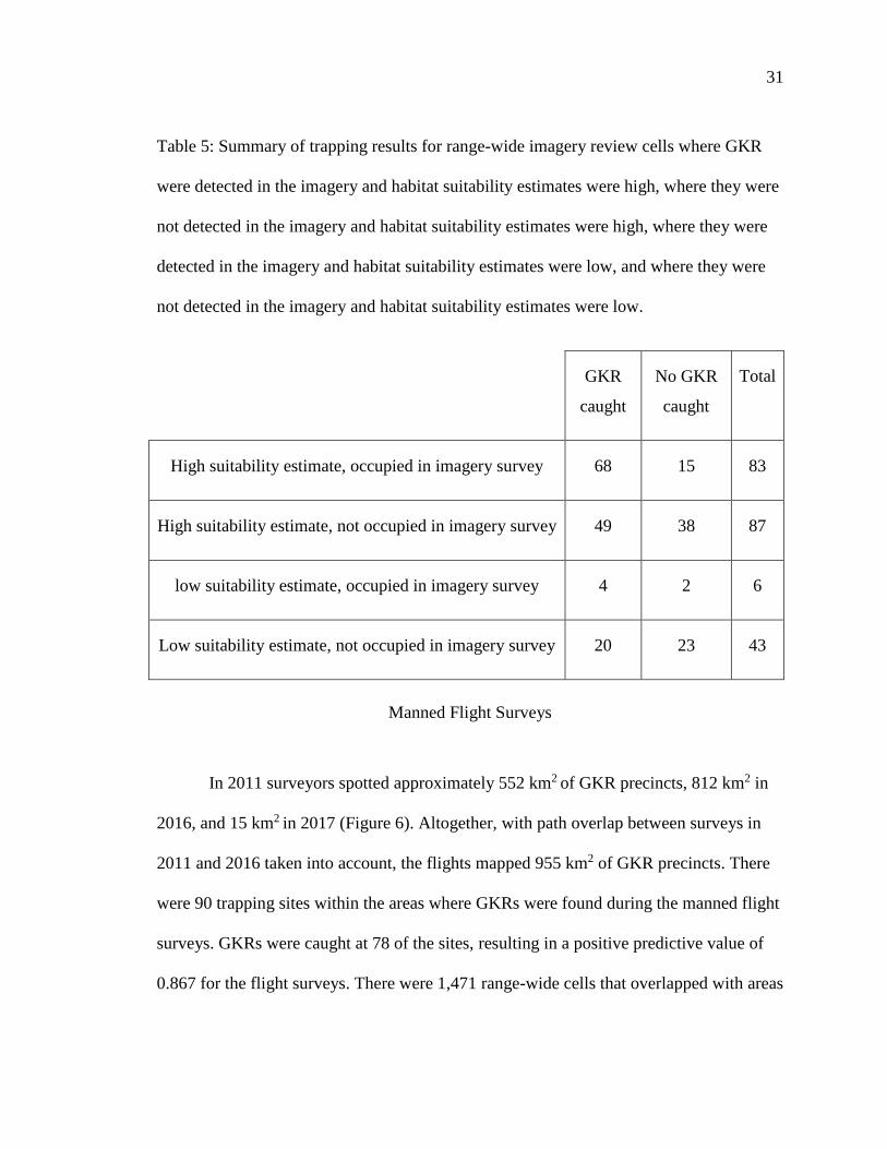
Trapping results were summarized for range-wide imagery review cells with high

habitat suitability estimates where GKR were detected in the imagery, low habitat

suitability estimates where GKR were detected in the imagery, high habitat suitability

estimates where GKR were not detected in the imagery, and low habitat suitability

estimates where GKR were not detected in the imagery. Only 49 of the 219 cells had low

habitat suitability estimates and GKR were detected in the range-wide imagery survey in

89 of the cells (Table 5). The category with the highest percentage of cells with GKR

captures was the high suitability estimate-occupied in imagery category, with 81.93%.

The percentages of cells with GKR captures in the high suitability estimate-not detected

in imagery, low suitability-GKR present in imagery, and low suitability-GKR not

detected in imagery categories were 56.32%, 66.67%, and 46.51%, respectively (Table

5).

31

Table 5: Summary of trapping results for range-wide imagery review cells where GKR

were detected in the imagery and habitat suitability estimates were high, where they were

not detected in the imagery and habitat suitability estimates were high, where they were

detected in the imagery and habitat suitability estimates were low, and where they were

not detected in the imagery and habitat suitability estimates were low.

GKR

caught

No GKR

caught

Total

High suitability estimate, occupied in imagery survey 68 15 83

High suitability estimate, not occupied in imagery survey 49 38 87

low suitability estimate, occupied in imagery survey 4 2 6

Low suitability estimate, not occupied in imagery survey 20 23 43

Manned Flight Surveys

In 2011 surveyors spotted approximately 552 km2 of GKR precincts, 812 km2 in

2016, and 15 km2 in 2017 (Figure 6). Altogether, with path overlap between surveys in

2011 and 2016 taken into account, the flights mapped 955 km2 of GKR precincts. There

were 90 trapping sites within the areas where GKRs were found during the manned flight

surveys. GKRs were caught at 78 of the sites, resulting in a positive predictive value of

0.867 for the flight surveys. There were 1,471 range-wide cells that overlapped with areas

32

where GKRs were detected in the manned flights. GKRs were present in satellite-aerial

image survey cells with scores ≥3 in 561 cells, resulting in a positive predictive value of

0.381 for flights when compared to the range-wide imagery review.

33

Figure 6: Historically suitable habitat as determined by a MaxEnt model thresholded to

the maximum sensitivity plus specificity (Rutrough et al. revised review) in

angled lines, locations where GKRs were observed during manned flight surveys

in light gray, range-wide imagery review cells where GKRs were observed with a

confidence of three or higher in dark gray, and sites where GKRs were trapped in

black.

34

UAV Surveys

The UAV utilized by this study was primarily used to select trapping locations.

During the summer of 2017, trapping locations were broadly influenced by the results of

the range-wide imagery surveys, but finer-scale decisions were made in the field. Using

the UAV to obtain an aerial view of general locations chosen for trapping proved to be a

quick and effective way to narrow down specific trapping sites. By observing the live

feed from the UAV, observers could note locations where there appeared to be GKR sign

and set traps in those areas. This proved to be quicker than searching broad areas on foot.

This study also aimed to use the UAV to systematic survey for GKR sign.

Unfortunately, there were some issues with the connection between the project’s UAV

and the controller, as well as some logistical difficulties that were not resolved until well

into the short field season due to the prioritization of other tasks. Because of these issues

there was not enough UAV data to conduct a formal analysis.

Sign Surveys

Seventeen variables from 163 sign surveys were used to build boosted regression

tree models to predict GKR presence according to trapping data (Elith et al. 2008).

Twenty-one models were built with learning rates between 0.0005 and 0.001 and

complexities between 4 and 6 (Appendix C). All models had a bag rate of 0because of the

35

small sample size (Elith et al. 2008). Many of the models performed similarly, but the

one with the lowest deviance was chosen for further assessment.

The best model had a complexity of 5 and a learning rate of 0.005. The model

accurately predicted GKR presence and absence according to the trapping data with a

cross validation AUC of 0.963 (SE = 0.014), sensitivity of 0.860 (SD = 0.073),

specificity of 0.842 (SD = 0.111), and true skill statistic of 0.702. The variables that

contributed the most to the model were tracks and tail drags, fresh aprons and non-

vegetative debris in burrows (relative influence = 36.971, 15.603, 8.164, respectively)

(Figure 7).

Figure 7: Relative influence for all variables used in boosted regression trees comparing

sign surveys to live trapping.

36

Models using sign survey data to predict GKR occupancy at the 85 sites that fell

within cells with confidence scores greater than or equal to 3 in the range-wide imagery

review were built using the same method as those testing the relationship with the

trapping data. The best model using range-wide imagery survey data had a complexity of

4 and a learning rate of 0.003. The model had a cross validation AUC of 0.780 (SE =

0.073), sensitivity of 0.883 (SD = 0.107), specificity of 0.962 (SD = 0.038), and true skill

statistic of 0.795. The variables that contributed the most to the model were fresh aprons,

tracks and tail drags, and mounds with burrows (relative influence = 18.378, 18.059,

10.216, respectively) (Figure 8).

Figure 8: Relative influence for all variables used in boosted regression trees comparing

sign surveys to range-wide imagery review results.

37

The sign survey data was augmented to create datasets were 5%, 10%, 25% and

50% of the sites where GKR were trapped were changed to indicate that no GKR were

caught in order to assess how sensitive boosted regression trees were to false absences.

Models run on the unaltered data had a higher average true skill statistic than those run on

the data with added false absences, and the true skill statistics declined as the percentage

of altered data increased (Table 6).

Table 6: Average sensitivity, specificity and true skill statistics for boosted regression

trees built with data that was purposely altered to introduce false absences. The

sensitivity and specificity of ‘observed’ results, achieved using altered data are compared

to the sensitivity of the same models run using ‘actual’ or unaltered data.

% of

captures

changed

to false

negatives

Average

‘observed’

sensitivity

Average

‘actual’

sensitivity

Average

‘observed’

specificity

Average

‘actual’

specificity

Average

‘observed’

true skill

statistic

Average

‘actual’

true skill

statistic

0 NA 0.860 NA 0.842 NA 0.702

5 0.842 0.861 0.775 0.823 0.617 0.684

10 0.825 0.861 0.747 0.883 0.572 0.694

25 0.724 0.862 0.707 0.828 0.431 0.689

50 0.268 0.860 0.867 0.834 0.135 0.694

Track Plates

Track plates were set alongside 140 traps on 27 plots. Small mammals were

38

detected by 119 of the track plates. Of these, 35 had large kangaroo rat tracks while the

remaining 84 had sign from other small mammals. Because kangaroo rats tend to walk on

their toes while moving slowly (Bartholomew & Caswell 1951), kangaroo rat tracks left

on the blotter paper were always incomplete. GKRs share their range with a similarly

sized sympatric species, the Heermann’s kangaroo rat (Dipodomys heermanni). While

GKRs have a significantly larger hind foot than D. heermanni (mean = 49.043 mm and

43.425 mm, respectively; t = 41.338, df = 677.64, p < 0.0001; 95% confidence interval =

(5.351, 5.885); A. Semerdjian, unpublished data), measurements for the two species were

indistinguishable without a complete track including the heel. After combining GKR and

Heermann’s kangaroo rats into a single ‘large kangaroo rat’ category, the specificity of

the track plates at both the site and trap scale were similar (specificity = 0.833 and 0.859,

respectively) (Table 7) though the sensitivity at the site level was much higher

(sensitivity = 0.952 and 0.458, respectively) (Table 8). The true skill statistics for these

tests were 0.785 and 0.317, respectively.

Table 7: Sites with large kangaroo rat tracks registered on track plates and the GKR and

Heermann’s kangaroo rat capture rate at those sites.

Large kangaroo rat caught No large kangaroo rat

caught

Large kangaroo rat tracks 20 1

No large kangaroo rat tracks 1 5

39

Table 8: Individual track plates with large kangaroo rat tracks and the capture rate of

GKR and Heermann’s kangaroo rats at the traps set next to each track plate.

Large kangaroo rat caught No large kangaroo rat

caught

Large kangaroo rat tracks 22 13

No large kangaroo rat tracks 26 79

40

DISCUSSION

GKRs were live trapped throughout their range to collect occurrence data and to

validate the findings of non-invasive methods. This study used aerial imagery to assess

GKR occupancy across their distribution and tested non-invasive techniques for

monitoring populations in the field. The range-wide imagery survey produced a coarse,

but exhaustive occupancy map for GKRs that identified several known and understudied

populations (Figures 5, 6). The high specificity and lower sensitivity indicate that GKRs

are likely present in most of the areas where they were identified in the range-wide

imagery review, but may also be present locations where they were not observed in the

imagery. Other aerial methods were used to evaluate GKR occupancy as well. The

manned flights outlined the boundaries of GKR populations in areas where surveys were

conducted. These surveys mostly matched trapping data, but were less correlated with the

results of the range-wide imagery review (Figure 6). The UAV surveys did not yield

results, but with few modifications the method could prove valuable for land managers.

Non-aerial, non-invasive methods included track plates and sign surveys. Track plates

were deployed at sites where live-trapping and sign surveys occurred. Kangaroo rat

tracks were collected on the plates at most locations, but these tracks could not be

identified to species. The sign surveys’ high sensitivity and specificity indicated that this

method predicted GKR presences and absences accurately, according to the trapping

data.

Live Trapping

41

Extensive live trapping occurred throughout the GKR range from 2010 to 2017.

The data from this effort contributed toward studies investigating GKRs genetic

connectivity (Alexander 2016, Statham et al. 2019), GKR habitat suitability (Bean et al.

2012a, Bean et al. 2014a, Bean et al. 2014b), and potential biotic and abiotic threats that

GKRs might face in the future (Widick 2018, Widick & Bean 2019). Ideally, trapping

sites would have been randomly distributed across areas with varying likelihoods of GKR

presence, but the majority of trapping sites were chosen for other projects and targeted

areas where GKRs were likely present. The only years where traps were set in areas with

a lower probability of capture were 2016 and 2017, when data was being collected

specifically for this study. This likely biases some of the comparative results. That being

said, the size of the trapping plots and the specific time period in which a GKR can be

detected in a location using traps makes this method the most spatially and temporally

accurate survey method used here. By trapping, this study was able to definitively locate

scattered GKR populations in the Panoche, monitor the edges of the population in the

Carrizo, and confirm the existence of under-studied colonies near Kettleman Hills and

north of the Carrizo.

Range-wide Imagery Survey

The ability to remotely survey a species’ entire range is uncommon, making the

range-wide imagery review a unique resource for managers interested in GKR

conservation. Predicting where GKRs are located within their range is difficult, in part

due to their historically patchy distribution, and in part because of the rapid development

42

and modification of their habitat (Grinnell 1932, Williams 1992). The range-wide

imagery review map serves as a starting point for identifying GKR presence in order to

make management decisions.

Habitat suitability models are another tool that managers use when deciding

where to focus conservation efforts. However, suitability does not always correlate with

occupancy, and vice versa (e.g. Pulliam 1988, Clevenger et al. 1997, Schlaepfer et al.

2002). Suitability models and occupancy maps for GKRs provide evidence of flaws in the

relationship. GKRs were reliably absent in the range-wide imagery review in places with

low habitat suitability estimates and the majority of the locations where GKRs were

observed in the imagery review fell within areas with high habitat suitability estimates.

However, much of the historical GKR range, though suitable in regards to abiotic

variables, was unoccupied (Figure 6). This is likely due in part to anthropogenic habitat

conversion and other abiotic interactions including conflicts with other rodent species

(Widick 2018, Widick & Bean 2019) and the domination of historically sparse vegetation

communities by non-native, thatch-producing grasses (Germano et al. 2001).

Mismatches between habitat suitability estimates and occupancy do not discount

the value of either factor for species conservation. For example, large tracts of land with

high habitat suitability estimates but no GKR detections are covered in invasive grasses

that preclude GKR establishment. Cattle grazing and other management tactics may be

used to restore these areas for use by GKR (Germano et al. 2012). Additionally, strategic

fallowing plans cooperatively formed by land managers and farmers in the San Joaquin

43

Valley deal with land that is, for the most part, unoccupied by species of conservation

concern (Butterfield et al. 2017). Occupancy in nearby areas should be a factor for these

plans, as some species, including GKRs, can recolonize fields without human assistance

(Blackhawk et al. 2016). However, habitat suitability models will ultimately determine

which parcels are of the highest value for endangered species, with areas with low

suitability estimates being ruled out for conservation purposes (Butterfield et al. 2017).

Habitat suitability models have also been used to identify locations in the San Joaquin

valley where development would substantially impact endangered species, including

GKRs, and to suggest areas that would meet development needs while incurring less

harm to sensitive species (Phillips & Cypher 2015).

Regardless of whether a location is considered good habitat, developers in the San

Joaquin Valley must conduct surveys to determine whether endangered species are

present on potential building sites (AEP 2018). In response to these surveys developers

may have to modify or scale back their projects to protect endangered species (O’Farrell

et al. 2016). Presence of endangered species is also a factor in deciding where mitigation

lands should be established following development (Fox & Nino-Murcia 2005). Though

habitat suitability models and species occupancy data are often used separately there is

far more to be gained by using them together. Mitigation, for example, would be more

impactful if long-term habitat suitability was taken into account as well as current species

occupancy. There have been several studies assessing GKR habitat suitability at different

temporal and spatial scales (Bean et al 2014b, Widick 2018, Widick & Bean 2019,

44

Rutrough et al. revised review), but this study is the first to assess occupancy throughout

their entire range.

The regions where GKRs were identified in the range-wide imagery review with

the highest levels of confidence include the well-studied populations in the Carrizo and

Panoche, as well as potential populations in the center of the GKR range near the

Kettleman Hills as well as in Wind Wolves Preserve and Cuyama Valley, which lies

south of the Carrizo. GKR presence has been confirmed by trapping in many of the areas

where they were detected remotely. During the course of this study they were live-

trapped in many locations throughout the Carrizo and Panoche, and were caught near the

Kettleman Hills. GKRs have been known to occur in the Cuyama Valley both historically

(Grinnell 1932), and within the last 30 years (Williams 1992). I was not granted

permission to conduct trapping or surveys in the region but, anecdotally, in the summer

of 2017 researchers observed apparently active GKR precincts along Aliso Canyon Rd, a

public road that transects the large patch where GKRs were detected in the range-wide

imagery survey in Cuyama Valley.

There were no active GKR precincts found at Wind Wolves Preserve despite high

confidence detections in the range-wide imagery review (figure 5, 6). During trapping

observers noted that there were mounds on the landscape, but any burrow entrances that

had been there were degraded beyond recognition. Reports from local managers suggest

that it is very unlikely that there are currently GKRs in the area. It is possible that forces

other than GKRs created the mounds, which were visible both on the ground and in aerial

45

imagery. However, Wind Wolves Preserve appears to be suitable habitat according to the

MaxEnt model built from historical records, so it is also possible that they occupied the

preserve in the past and have been extirpated (figure 6).

If a precinct is occupied over a long duration the burrow system will eventually

develop a mound due to the continuous displacement of soil. In one example, banner-

tailed kangaroo rats (Dipodomys spectabilis) in New Mexico developed mounds over 30

cm tall between 23 and 30 months after colonizing a new area (Best 1972). The mounds

deteriorated after approximately a year following the removal of kangaroo rats (Best

1972) but in some cases kangaroo rat mounds can remain detectable for a decade or more

after abandonment (J. Chestnut, personal communication 30 August 2018). The rate of

deterioration likely depends on factors including the size of the mound, the length of

occupation, and environmental variables including soil quality, vegetation, and amount of

precipitation.

The results of the boosted regression trees predicting range-wide imagery survey

results from on-the-ground sign survey transects distinguished mounds as one of the three

most influential variables, suggesting that along with other signs of active use, the

topographic features of precincts play heavily into observers’ ability to see them in aerial

imagery. An inherent limitation of the range-wide imagery review method is that some of

the detected precincts, potentially including the mounds at Wind Wolves Preserve, may

have been unoccupied when the imagery was gathered. However, because conditions

would have to support GKRs for several years in order mounds to be visible in imagery

46

review, those areas likely are or were suitable for a long time. Therefore these detections

offer information about GKR habitat needs, even if GKRs are not currently present.

Depending on the reason for extirpation, these areas may be candidates for restoration or

GKR reintroduction.

The influence of mounds for detecting GKRs in the range-wide imagery survey

poses another limitation. Not all occupied precincts are mounded, and mounds are not the

only sign that is visible in the imagery. A post-hoc review of 50 range-wide imagery

review cells that contained trapping sites revealed that precincts that were not visible in

the 2008 and 2014 imagery that we utilized, are clearly detectable in the imagery taken in

2017 (Maxar Technologies 2017). Out of the 50 cells that were revisited, GKRs were not

detected in 2 of the cells where they had been called present in the initial survey, and

GKRs were detected in 16 cells where they had previously been absent. On average the

review differed from the initial assessment by 3.5 confidence points. GKR distributions

have been known to fluctuate according to climatic conditions, and because the older

imagery is from drier years (PRISM 2004), it is possible that GKR populations were

simply not as widespread when the imagery was captured. It is also possible that GKR

sign was simply more visible in the newer imagery. The effects that GKR have on

vegetation would be more visible in years with higher rainfall because the rain would

cause uneaten seeds in pit caches to germinate, resulting in thicker vegetation on

precincts than in surrounding areas, and because there would be more vegetation

surrounding precincts to contrast with the bare soil after GKR clip the vegetation around

their burrows in late spring and early summer. Because of fluctuating population

47

boundaries and vegetation effects, it is likely that the results of the range-wide imagery

survey would be different, and possibly more reflective of the trapping data, if it were

conducted again using imagery from years with more precipitation.

Manned Flight Surveys

Another limitation of the range-wide imagery review is that precincts in shrubby

areas may be harder to detect. The GKR population at Lokern is well documented

(Germano & Saslaw 2017) but most of the GKR presences noted in the range-wide

imagery review in that area had low confidence. A larger portion of the colony was

identified in the manned flight surveys (figure 6). While the range-wide imagery review

observations rely heavily on precinct topography, observers for the manned flight survey

focus on spotting bare patches caused by GKR vegetation clipping on precincts. Because

the flight surveys rely on sign created during the year of the survey they have a finer

temporal scale than the range-wide imagery review, and because they occur at a lower

altitude observers can spot precincts that are harder to find in lower resolution imagery.

The flight surveys corresponded to the trapping data better than they did to the

range-wide imagery review. This may be in part due to similarities in temporal precision,

as previously addressed, but bias in the placement of trapping sites is a likely factor as

well. Most of trapping sites in the Carrizo, which is where the bulk of the sites used to

analyze the flight surveys came from, were chosen to maximize the likelihood of catching

48

GKRs. Future research investigating whether flight surveys reflect trapping data for GKR

should utilize trapping sites set in areas with varying likelihoods of GKR capture.

UAV Surveys

Manned flight surveys, though effective for monitoring GKR populations, may

pose a risk to the pilots and biologists on board the small, low flying aircrafts and are

limited by time and funding. UAV surveys may be a viable alternative. Unfortunately this

study experienced technical difficulties resulting in insufficient data to analyze the

effectiveness of UAV surveys. Anecdotally however, the UAV was useful for locating

GKR precincts when they were active and densely clustered, but it was difficult to

confidently identify them when they were sparse. While the UAV imagery could not be

used to perfectly detect GKRs it was useful for detecting abundant activity, and

identifying areas of interest for further investigation.

Advice for those interested in using UAVs to located GKRs in the future includes

purchasing a UAV with the capability to connect with its controller over long distances.

The UAV used for this project experienced issues moving more than 50 meters vertically

or 500 meters horizontally from the controller before it lost connection and automatically

returned to the start point. The problem did not affect pre-programmed surveys, but it

limited the utility of exploratory flights. In addition, while the Litchi app was functional

for creating pre-programmed flights, there are programs with more useful features for

people surveying large parcels. DroneDeploy (Infatics, Inc. 2018), for example, has more

49

integrated functions for designing transects and splicing photographs to create a single

image of the survey location. With protocol modifications, a UAV would be a useful tool

for managers or researchers to identify possible GKR sign over areas too large to

thoroughly survey on foot. Without further testing, however, any sign identified using

UAVs should be verified using a secondary method.

Sign Surveys

Though trapping is considered the most reliable way to determine GKR

occupancy, it is likely that occasionally GKR will not be trapped on sites where they are

active. In order to test whether the sign survey analysis is sensitive to false negatives,

datasets with artificial false absences were created. With the acknowledgement that

trapping data used to build the original sign survey models likely already included some

unidentified false absences, analysis showed that sensitivity and specificity generally

declined as false negatives increased (Table 6). Additionally, the same models that were

used to predict GKR presence using the altered data had higher sensitivity and specificity

values that were similar to those calculated using the top model for the unaltered data.

Sensitivity and specificity are a measure of false presences and absences, respectively.

Values decreasing as data is artificially falsified tells us that the model is predicting GKR

presences and absences even when the data disagrees. The decline in accuracy measures

when the data is falsified coupled with the stable measures when unaltered data is used

tells us that boosted regression trees are robust to false negatives in GKR trapping data,

further proving the predictive power of this method.

50

The sign surveys performed well when compared to both trapping data and the

range-wide imagery review. Fresh aprons and tracks and tail drags were among the top

three influential variables in both tests. Dirt that was recently kicked out of a burrow

opening and tracks are both signs of recent occupation, as wind and other disturbances

can quickly degrade GKR sign. The third most influential variable for the test predicting

trapping data from the sign surveys was non-vegetative debris in burrow openings. GKRs

regularly maintain their precincts, including clearing clutter from burrow openings.

Debris accumulation in burrows can indicate that they are absent, or less active at the site.

GKRs spend considerable time underground (Braun 1985) and therefore may be present

but not active above ground for extended periods. Because trapping only occurs at each

site for a few days, GKR need to be active above ground in a relatively short time span in

order to be caught. The sign surveys picked on details that can change over short

timespans, matching nicely with the trapping data.

Fine-scale absences or occupancy turn over may not contribute significantly to the

range-wide imagery review results. Mounding on burrow complexes occurs over a broad

timespan. Mounds barely contributed to the results of the sign survey-trapping

comparison, but they featured heavily when the sign surveys were compared to the range-

wide imagery review. Mounds indicate that a colony persisted on the landscape for at

least long enough for dirt to accumulate over burrows, but they do not necessarily signify

current occupancy. By incorporating recent sign with long-term sign, the sign surveys

offer insight into both long term and short-term occupancy, predicting both fairly

accurately using slightly different models.

51

In addition to accurately predicting GKR occupancy, the sign survey protocol is

based on binary determinations of sign presence with no quantification involved, making

it less subjective. The survey was also designed to be easy to learn, regardless of whether

observers have had past experience with GKR monitoring. They required fairly little

effort and compared to live trapping, and were significantly faster. In addition,

conducting sign surveys instead of trapping reduces stress on GKRs because animals are

not caught or handled, and requires fewer site visits, therefore reducing trampling of

habitat.

In most modeling situations sensitivities and specificities exceeding 0.80 would

be considered accurate. However, it is important to note that in this case a sensitivity of

0.860 means that GKRs were not trapped at 14% of sites where the survey predicted that

they would be and a specificity of 0.842 means that they were caught at 15.8% of sites

where they survey predicted they were absent. This margin may be unacceptable

depending on the context for which the surveys are being used. Conducting several

surveys on the same parcel may help overcome the issue of false presences and absences.

Additionally, those collecting data from many surveys over large areas may want to

include some trapping sites to verify their results. Overall though, the sign surveys will be

very useful for managers as a non-subjective, low impact, inexpensive and quick way to

determine GKR presence.

52

Track Plates

Track plates were deployed with live-traps at sites in the south part of the GKR

range during the 2017 trapping season. There was little concern of the track plates

affecting trapping outcomes or vice-versa. The track plates did not restrain animal, so

they could easily visit the track plate and then go into a trap. Conversely, the traps were

ideally checked and closed several hours before dawn, so if a kangaroo rat was caught in

a trap it is likely that it would be released and still have time to find its way back to a

track plate that night.

The track-plate design (Figure 3; Appendix B) worked well in the field. The

charcoal-mineral oil mixture did not evaporate off of the felt pads, even when exposed to

extreme heat and served as effective ink that produced clear tracks. It is not uncommon to

find sign from kit foxes, coyotes and ravens on or near traps, and occasionally traps are

rolled over or moved. However, very few of the gutter constructions were moved or

seriously disturbed due to the use of eyebolts and railroad spikes to secure the plates to

the ground. The few times that the track plates were moved were likely the result of

larger animals like cows investigating them.

The plates clearly picked up prints from kangaroo rats, but, because kangaroo rats

walk on their toes when moving slowly, the tracks did not include the entire foot. Though

Heermann’s kangaroo rats, which co-occur with GKRs in many locations, have smaller

feet, their tracks were indistinguishable when incomplete. The track plate results were

53

strongly related to capture success for these two large kangaroo rat species at a site level,

and only two of the 27 plots with track plates had conflicting track plate-trapping results.

Track plate and trapping were also related at the trap-location level, however the high

specificity and low sensitivity suggests that this relationship is driven by locations where

large kangaroo rats were not detected in either method, rather than locations where they

were detected in both.

Though they can occupy similar habitat, Heermann’s kangaroo rats do not build

precinct complexes and their sign is not as conspicuous as GKR. Many of the sign

surveys took place in locations where Heermann’s kangaroo rats were caught, but no

GKR were, and the accuracy of the results seem to reflect the difference in the sign they

create. The track plates, though limited in application, could potentially be used along

with sign surveys or non-invasive methods with less temporal certainty to determine

current kangaroo rat occupancy.

54

CONCLUSIONS

The range-wide imagery survey provides an unprecedented complete census of

the GKR range and despite some notable cases of sign not being detected in areas where

GKRs are known to be present, as well as false presences, the survey provides a key

foundation for assessing the distribution of GKRs. The range-wide imagery review is

especially suitable for investigating GKR distribution at a broad-scale when paired with

habitat suitability models. GKRs were trapped with roughly a 77% success rate in

locations where GKRs were present in the imagery review and habitat suitability

estimates were high. These results represent a starting point for prioritizing land

acquisition for GKR conservation, potentially illustrating the importance of previously

overlooked populations and saving time and energy for those considering large areas.

Specifically, habitat suitability estimates, the range-wide imagery review, and the

manned flight surveys all indicate that Cuyama Valley and Sunflower Valley, just west of

the Kettleman Hills, are areas that managers may want investigate in the future.

The methods tested in this study varied widely in the temporal and spatial scale at

which GKR were detected. Live trapping, sign surveys and track plates utilized the same

plots, and therefore sampled the same amount of habitat, though the exact effective

sampling area can be difficult to determine. These methods are the most limited in the

extent to which results can be extrapolated into the surrounding area. It would be risky to

assume that a GKR detection at a plot set in a heterogeneous environment indicates that

they occupy the surrounding area. However, if GKRs are trapping in an area that appears

55

to have abundant GKR activity, the occupied area may potentially be projected to include

the colony in which the trapping site was set. The effective area of a trapping site, and

therefore the sign surveys, since they were conducted in the same locations, depends

largely on where the plots are set. In principle the same risk of assuming GKR are present

in areas that were not surveyed may apply to the UAV and flight surveys. However,

because more data can be gathered over a large area using these aerial methods,

extrapolations can be better informed. Finally, because the range-wide imagery review

covers the GKRs entire range, though at a coarse scale, there is theoretically no habitat

where likelihood of presence needs to be estimated.

In addition to operating at different spatial scales, the temporal coverage of these

methods differs as well. From finest to coarsest, GKR detected during live trapping had

to be active on the plot they were caught the night they were caught. The age of tracks

left on track plates will depend on how long the track plates are left in the field, which is

in this study was up to three nights. Observers were instructed to record fresh sign during

sign surveys, though perception of freshness likely depends largely on how quickly the

environment degrades it. Because GKR live in areas that are typically hot and often

windy, most sign likely degrades in less than a week, which would reflect the maximum

time since last activity that would be detected using the sign surveys. The data recorders

for the UAV and manned flight surveys are instructed to look for fresh GKR sign, which

from high altitude largely include grass clipping. Without clipping, vegetation would

appear thicker, or the same as the areas surrounding precincts, so GKR sign would not be

detected using these methods if GKRs were not actively maintaining burrows at least

56

through the spring before the surveys. Finally, the range-wide imagery surveys detect

GKR sign over the longest time period because the topographic features of GKR

precincts are highly visible in high altitude aerial imagery, and mounds can persist for a

long time after GKR have been extirpated.

Which of these methods are used would likely depend on the management goal as

well as the time and resources available. Agreement between two or more surveys,

including the range-wide imagery review, would offer a fair degree of confidence in

whether an area is occupied by GKRs, which could be estimated by multiplying the

probability of occupancy as determined by each method. In the case of a very large area

of interest, using aerial methods first and then conducting sign surveys in locations with

contrasting results may be sufficient to ascertain occupancy. In the case of hopelessly

unresolved disagreement between non-invasive methods, trapping may be necessary.

Comprehensive occupancy data for GKRs collected using comparable survey

methods is limited. Perhaps the greatest potential of the non-invasive methods in this

study lies in the ability to implement a standardized version of them. Standardizing data

collection across the GKR range will result in a better understanding of their distribution

and population dynamics across time. With these tools, entities tasked with conserving

GKRs will be able to communicate more clearly to provide for the species into the future.

57

LITERATURE CITED

Alexander, N. 2016. Genetic structure and connectivity of the endangered giant kangaroo

rat (Dipodomys ingens) in a heterogeneous environment. Thesis, Humboldt State

University, California, USA.

Allouche, O., A. Tsoar & R. Kadmon. 2006. Assessing the accuracy of species

distribution models: prevalence, kappa and the true skill statistic (TSS). Journal of

Applied Ecology 43: 1223-1232.

Araújo, M.B. & A.T. Peterson. 2012. Uses and misuses of bioclimatic envelope

modeling. Ecology 93: 1527-1539.

Araújo, M.B., R.J. Whittaker, R.J. Ladle & M. Erhard. 2005. Reducing uncertainty in

projections of extinction risk from climate change. Global Ecological Biogeography

14: 529-538.

Association of Environmental Professionals (AEP). 2018. 2018 California Environmental

Quality Act (CEQA) Statute and Guidelines. Palm Desert, CA.

Balmford, A., J.L. Moore, T. Brooks, N. Burgess, L.A. Hansen, P. Williams, & C.

Rahbek. 2001. Conservation conflicts across Africa. Science 291: 2616-2619.

Bartholomew, G.A., Jr & H.H. Caswell, Jr. 1951. Locomotion in kangaroo rats and its

adaptive significance. Journal of Mammalogy 32: 155-169.

58

Bean. W.T., L.R. Prugh, R. Stafford, H.S. Butterfield, M. Westphal & J.S. Brashares

2014a. Species distribution models of an endangered rodent offer conflicting

measures of habitat quality at multiple scales. Journal of Applied Ecology 51: 1116-

1125.

Bean, W.T., R. Stafford, & J.S. Brashares. 2012a. The effects of small sample size and

sample bias on threshold selection and accuracy assessment of species distribution

models. Ecography 35: 250-258.

Bean, W. T., R. Stafford, H. S. Butterfield & J. S. Brashares. 2014b. A multi-scale

distribution model for non-equilibrium populations suggests resource limitation in an

endangered rodent. PLoS ONE 9: 1-9.

Bean, W.T., R. Stafford, L.R. Prugh, H.S. Butterfield & J.S. Brashares. 2012b. An

evaluation of monitoring methods for the endangered giant kangaroo rat. Wildlife

Society Bulletin 36: 587-593.

Best, T.L. 1972. Mound development by a pioneer population of the banner-tailed

kangaroo rat Dipodomys spectabilis baileyi Goldman, in Eastern New Mexico. The

American Midland Naturalist 87: 201-206.

Blackhawk, N. C., D. J. Germano & P. T. Smith. 2016. Genetic variation among

populations of the endangered giant kangaroo rat, Dipodomys ingens, in the southern

San Joaquin Valley. American Midland Naturalist 175: 261-274.

59

Braun, S.E. 1985. Home range and activity patterns of the giant kangaroo rat, Dipodomys

ingens. Journal of Mammalogy 66: 1-12.

Brehme, C.S., L.R. Albert, T.A. Matsuda, R.N. Booth & R.N. Fisher. 2010. Pacific

pocket mouse sampling methodology study, Marine Corps Base, Camp Pendleton.

Prepared for AC/S Environmental Security, Marine Corps Base, Camp Pendleton.

47p.

Brooks, T.M., R.A. Mittermeier, G.A.B. da Fonseca, J. Gerlach, M. Hoffmann, J.F.

Lamoreux, C.G. Mittermeier, J.D. Pilgrim, & A.S.L. Rodrigues. 2006. Global

biodiversity conservation priorities. Science 313: 58-61.

Butterfield, H.S., R. Kelsey, A. Hart, T. Biswas, M. Kramer, D. Cameron, L. Crane, and

E. Brand. 2017. Identification of potentially suitable habitat for strategic land

retirement and restoration in the San Joaquin Desert. Unpublished report. The Nature

Conservancy, San Francisco, California. 25 pages.

California Division of Oil, Gas and Geothermal Resources (CDOGGR). 2016. AllWells.

[Shapefile geospatial data]. http://www.conservation.ca.gov/dog/geothermal/maps

California Protected Area Database (CPAD). 2017. www.calands.org.

Cooper, L.D. & J.A. Randall. 2007. Seasonal changes in home ranges of the giant

kangaroo rat (Dipodomys ingens): A study of flexible social structure. Journal of

Mammalogy 88: 1000-1008.

60

Clevenger, A.P., F.J. Purroy & M.A. Campos. 1997. Habitat assessment of a relict brown

bear Ursus arctos population in northern Spain. Biological Conservation 80:17-22.

Crowder, L.B., S.J. Lyman, W.F. Figueria & J. Priddy. 2000. Source-sink population

dynamics and the problem of siting marine reserves. Bulletin of Marine Science 66:

799-820.

Cui, S., J. Milner-Gulland, N.J. Singh, H. Chu, C. Li, J. Chen & Z. Jiang. 2017. Historical

range, extirpation and prospects for reintroduction of saigas in China. Scientific

Reports 7: 44200.

D’Elia, J., S.M. Haig, M. Johnson, B.G. Marcot & R. Young. 2015. Activity-specific

ecological niche models for planning reintroductions of California condors

(Gymnogyps californianus). Biological Conservation 184: 90-99.

Elith, J., J.R. Leathwick & T. Hastie. 2008. A working guide to boosted regression trees.

Journal of Animal Ecology 77: 802-813.

Eriksson, O. 1996. Regional dynamics of plants: a review of evidence for remnant,

source-sink and metapopulations. Oikos 77: 248-258.

Fox, J. & A. Nino-Murcia. 2005. Status of species conservation banking in the United

States. Conservation Biology 19: 996-1007.

61

Freeman, E.A. & G. Moisen. 2008. PresenceAbsence: An R package for presence-

absence model analysis. Journal of Statistical Software 23: 1-31.

http://www.jstatsoft.org/v23/i11

Germano, D.J., G.B. Rathbun & L.R. Saslaw. 2001. Managing exotic grasses and

conserving declining species. Wildlife Society Bulletin 29: 551-559.

Germano, D.J., G.B. Rathbun & L.R. Saslaw. 2012. Effects of grazing and invasive

grasses on desert vertebrates in California. The Journal of Wildlife Management 76:

670-682.

Germano, D.J. & L.R. Saslaw. 2017. Rodent community dynamics as mediated by

environment and competition in the San Joaquin Desert. Journal of Mammalogy 98:

1615-1626.

Glennon, M.J., W.F. Porter & C.L. Demers. 2002. An alternative field technique for

estimating diversity of small-mammal populations. Journal of Mammalogy 83: 734-

742.

Gompper, M.E., R.W. Kays, J.C. Ray, S.D. Ladpoint, D.A. Bogan & J.R. Cryan. 2006. A

comparison of non-invasive techniques to survey carnivore communities in

northeastern North America. Wildlife Society Bulletin 34: 1142-1151.

62

Greene, K., D. Bell, J. Kioko & C. Kiffner. 2017. Performance of ground-based and

aerial survey methods for monitoring wildlife assemblages in a conservation area of

northern Tanzania. European Journal of Wildlife Research 63: 77.

Greenwell, B., B. Boehmke, J. Cunningham & GBM Developers. 2018. gbm:

Generalized Boosted Regression Models. R package version 2.1.4. https://CRAN.R-

project.org/package=gbm

Grinath, J.B., N. Deguines, J. W. Chestnut, L. R. Prugh, J. S. Brashares & K. N. Suding.

2018. Animals alter precipitation legacies: Trophic and ecosystem engineering effects

on plant community temporal dynamics. Journal of Ecology 00: 1-16.

Grinnell, J. 1932. Habitat relations of the giant kangaroo rat. Journal of Mammalogy 13:

305-320.

Guisan, A. & W. Thuiller. 2005. Predicting species distribution: offering more than

simple habitat models. Ecology Letters 8: 993-1009.

Guisan A., R. Tingley, J.B. Baumgartner, I. Naujokaitis-Lewis, P.R. Sutcliff, A.I.T.

Tulloch, T.J. Regan, L. Brotons, E. McDonald‐Madden, C. Mantyka‐Pringle, T.G.

Martin, J.R. Rhodes, R. Maggini, S.A. Setterfield, J. Elith, M.W. Schwartz, B.A.

Wintle, O. Broennimann, M. Austin, S. Ferrier, M.R. Kearney, H.P. Possingham,

Y.M. Buckley. 2013. Predicting species distributions for conservation decisions.

Ecology Letters 16: 1424-1435.

63

Guisan A. & N.E. Zimmerman. 2000. Predictive habitat distribution models in ecology.

Ecological Modelling 135: 147-186.

Hijmans, R.J. & C.H. Graham. 2006. The ability of climate envelope models to predict

the effect of climate change on species distributions. Global Change Biology 12:

2272-2281.

Hodgeson, J.C., S.M. Baylis, R. Mott, A. Herrod & R.H. Clarke. 2015. Precision wildlife

monitoring using unmanned aerial vehicles. Scientific Reports 6: 22574.

Homer, C.G., Dewitz, J.A., Yang, L., Jin, S., Danielson, P., Xian, G., Coulston, J.,

Herold, N.D., Wickham, J.D., and Megown, K., 2015, Completion of the 2011

National Land Cover Database for the conterminous United States-Representing a

decade of land cover change information. Photogrammetric Engineering and Remote

Sensing, v. 81, no. 5, p. 345-354

Hubbs, A.H., T. Karels & R. Boonstra. 2000. Indices of population size for burrowing

mammals. The Journal of Wildlife Management 64: 296-301.

Hutchinson, G.E. 1957. Concluding remarks. Cold Spring Harbor Symposia on

Quantitative Biology 22: 145-159.

Infatics, Inc. 2018. DroneDeploy – Mapping for DJI (Version 2.80.0) [Mobile application

software].

64

Johnston, A., D. Fink, M.D. Reynolds, W.M. Hochachka, B.L. Sullivan, N.E. Bruns, E.

Hallstein, M.S. Merrifield, S. Matsumoto & S. Kelling. 2015. Abundance models

improve spatial and temporal prioritization of conservation resources. Ecological

Applications 25: 1749-1756.

Jones, W.T. 1993. The social systems of heteromyid rodents. Pp. 575–595 in Biology of

the Heteromyidae (H. H. Genoways and J. H. Brown, eds.). Special Publication 10,

The American Society Of Mammalogists.

Kay, F.R. & W.G. Whitford. 1978. The burrow environment of the banner-tailed

kangaroo rat, Dipodomys spectabilis, in south central New Mexico. The American

Midland Naturalist 99: 270-279.

Kellner, C.J., J.D. Brawn, & J.R. Karr. 1992. What is habitat suitability and how should it

be measured? Pages 476-488 in Wildlife 2001: populations. Springer, Dordrecht.

Lentini, P.E., I.A. Stirnemann, D. Stojanovic, T.H. Worthy & J.A. Stein. 2018. Using

fossil records to inform reintroduction of the kakapo as a refugee species. Biological

Conservation 217: 157-165.

Margules C.R. & R.L. Pressey. 2000. Systematic conservation planning. Nature 405:

243-253.

Maxar Technologies. 2017. DigitalGlobe - https://www.digitalglobe.com/

65

Meineri, E., A.S. Deville, D. Grémillet, M. Gauthier-Clerc, & A. Béchet. 2014.

Combining correlative and mechanistic habitat suitability models to improve

ecological compensation. Biological Reviews 90: 314-329.

Murie, O.J. & M. Elbroch. 2005. Peterson field guide to animal tracks. 3rd ed. Houghton

Mifflin Harcourt.

Naidoo, R., A. Balmford, P.J. Farraro, S. Polasky, T.H. Ricketts, & M. Rouget. 2006.

Integrating economic costs into conservation planning. Trends in Ecology and

Evolution 21: 681-687.

O’Farrell, T.P., N.E. Mathews, P.M. McCue & M.S. Kelly. 2016. Distributions of the

endangered giant kangaroo rat, Dipodomys ingens, on the Naval Petroleum Reserves,

California. (No. EGG-10282-2173). EG and G Energy Measurements, Inc., Goleta,

CA (USA). Santa Barbara Operations.

Pearson, R.G. & T.P. Dawson. 2003. Predicting the impacts of climate change on the

distribution of species: are bioclimate envelope models useful? Global Ecology &

Biogeography 12: 361-371.

Phillips, S.E. & B.L. Cypher. 2015. Solar energy development and endangered upland

species of the San Joaquin Valley: Identifications of conflict zones. Prepared for: The

California Department of Fish and Wildlife Agreement: P1440003 00.

PRISM Climate Group, Oregon State Univeristy, http://prism.oregonstate.edu, created 4

Feb 2004.

66

Prugh, L. R. & J. S. Brashares. 2012. Partitioning the effects of an ecosystem engineer:

kangaroo rats control community structure via multiple pathways. Journal of Animal

Ecology 81: 667-678.

Prugh, L.R., N. Deguines, J.B. Grinath, K.N. Suding, W.T. Bean, R. Stafford & J.S.

Brashares. 2018. Ecological winners and losers of extreme drought in California.

Nature Climate Change 8: 819-824.

Pulliam, H.R. 1988. Sources, sinks, and population regulation. The American Naturalist

132: 652-661.

Pulliam, H. R. 2000. On the relationship between niche and distribution. Ecology Letters

3: 349-361.

Puttock, A.K., A.M. Cunliffe, K. Anderson & R.E. Brazier. 2015. Aerial photography

collected with a multirotor drone reveals impact of Eurasian beaver reintroduction on

ecosystem structure. Journal of Unmanned Vehicle Systems 3: 123-130.

Questad, E.J., J.R. Kellner, K. Kinney, S. Cordell, G.P. Asner, J. Thaxton, J. Diep, A.

Uowolo, S. Brooks, N. Inman-Narahari, S.A. Evans & B. Tucker. 2014. Mapping

habitat suitability for at-risk plant species and its implications for restoration and

reintroduction. Ecological Applications 24: 385-395.

R Core Team. 2018. R: A language and environment for statistical computing. R

Foundation for Statistical Computing, Vienna, Austria. URL https://www.R-

project.org/.

67

Rocchini, D., D.S. Boyd, J.B. Féret, G.M. Foody, K.S. He, A. Lausch, H. Nagendra, M.

Wegmann & N. Pettorelli. 2015. Satellite remote sensing to monitor species diversity

and potential pitfalls. Remote Sensing in Ecology and Conservation 2: 25-36.

Rutrough, A. I.V. Widick & W.T. Bean. revised review. Reconstruction of the historical

range alters niche estimates for an endangered rodent.

Schooley, R.L. & J.A. Wiens. 2001. Dispersion of kangaroo rat mounds at multiple scales

in New Mexico, USA. Landscape Ecology 16: 267-277.

Scheele, B.C., C.N. Foster, S.C. Banks & D.B. Lindenmayer. 2017. Niche contractions in

declining species: mechanisms and consequences. Trends in Ecology and Evolution

32: 346-355.

Schlaepfer, M.A., M.C. Runge & P.W. Sherman. 2002. Ecological and evolutionary

traps. Trends in Ecology and Evolution 17: 474-480.

Shaw, W.T. 1934. The ability of the giant kangaroo rat as a harvester and storer of seeds.

Journal of Mammalogy 15: 275-286.

Sikes, R.S., W.L. Gannon & The Animal Care and Use Committee of the American

Society of Mammalogists. 2011. Guidelines of the American Society of

Mammalogists for the use of wild animals in research. Journal of Mammalogy 92:

235-253.

68

Smyser, T.J., R.J. Guenzel, C.N. Jaques & E.O. Garton. 2016. Double-observer

evaluation of pronghorn aerial line-transect surveys. Wildlife Research 43: 474-481.

Statham, M.J., W.T. Bean, N. Alexander, M. F. Westphal, & B. Sacks. 2019. Historical

population size change and differentiation of relict populations of the endangered

giant kangaroo rat. Journal of Heredity, esz006, https://doi-

org.ezproxy.humboldt.edu/10.1093/jhered/esz006

Stanley, T.R. & J.A. Royle. 2005. Estimating site occupancy and abundance using

indirect detection indices. Journal of Wildlife Management 69: 874-883.

Stephenson, N. 1998. Actual evapotranspiration and deficit: biologically meaningful

correlates of vegetation distribution across spatial scales. Journal of Biogeography 25:

855-870.

Stockwell, D.R.B. & A.T. Peterson. 2002. Effects of sampling size on accuracy of

species distribution models. Ecological Modeling 148: 1-13.

Sutherland, W.J., A.S. Pullin, P.M. Dolman, & T.M. Knight. 2004. The need for

evidence-based conservation. Trends in Ecology and Evolution 19: 305-308.

SZ DJI Technology Co., Ltd. 2018. DJI GO (Version 3.1.42) [Mobile application

software]. Retrieved from http://itunes.apple.com.

U.S. Fish and Wildlife Service (USFWS). 1998. Recovery plan for the upland species of

the San Joaquin Valley, California. U.S. Fish and Wildlife Service, Portland, Oregon.

69

U.S. Fish and Wildlife Service (USFWS). 2010. Giant kangaroo rat (Dipodomys ingens)

5-year review: summary and evaluation. U.S. Fish and Wildlife Service, Sacramento,

California.

Van Horne, B., R.L. Schooley, S.T. Knick, G.S. Olson & K.P. Burnham. 1997. Use of

burrow entrances to indicate densities of Townsend’s ground squirrels. The Journal of

Wildlife Management 61: 92-101.

Vermeulen, C., P. Lejeune, J. Lisein, P. Sawadogo, P. Bouché. 2013. Unmanned aerial

survey of elephants. PloS one: e54700.

VC Technology Ltd. 2018. Litchi for DJI Drones (Version 2.5.1) [Mobile application

software]. Retrieved from http://itunes.apple.com.

Weissensteiner, M.H., J.W. Poelstra & J.B.W. Wolf. 2015. Low-budget ready-to-fly

unmanned aerial vehicles: an effective tool for evaluation the nesting status of

canopy-breeding bird species. Journal of Avian Biology 46: 425-430.

Widick, I., & W.T. Bean. 2019. Evaluating current and future range limits of an

endangered, keystone rodent (Dipodomys ingens). Diversity and Distributions 00: 1-

14.

Widick, I. 2018. Evaluating current and future range limits of an endangered, keystone

rodent (Dipodomys ingens). Thesis, Humboldt State University, California, USA.

70

Williams, D. F. 1992. Geographic distribution and population status of the giant kangaroo

rat, Dipodomys ingens (Rodentia, Heteromyidae). Endangered and Sensitive Species

of the San Joaquin Valley, California: Their biology, management and conservation

(D. F. Williams, S. Byrne & T. A. Rado, eds.). California Energy Commission,

California State University, Bakersfield.

Wilson, K.A., M.I. Westphal, H.P. Possingham & J. Elith. 2005. Sensitivity of

conservation planning to different approaches to using predicted species distribution

data. Biological Conservation 22: 99-112.

71

APPENDICES

Appendix A: Sign categories recorded during non-invasive GKR surveys.

Sign type Description

Grass clipping Vegetation at survey point is clipped a couple of inches

above the ground.

Haystacks Pile of seeds and grass stalks on bare ground. Can be a

couple of inches in diameter to a couple of meters.

Fresh apron Pile of fresh dirt splayed out of a burrow entrance.

Tracks and tail drags Kangaroo rat tracks include oblong parallel imprints from

hind feet. May or may not include lines in the dirt from

their tails dragging as they move slowly.

Pit caches Tablespoon size imprints where GKRs stored seeds. There

are often several in close proximity. Can cover the majority

of the bare dirt around a precinct.

Scats Smooth, slightly crescent shaped oblong scats measuring at

least 1.5x5 mm, which is the size of the smallest scat

collected from a GKRs during live trapping.

Runways Narrow trails in the grass connecting burrows or precincts.

Miscellaneous signs of

digging

Signs of digging that do not fall into the other categories

listed here.

Large mound with burrows Raised earth with one to several burrow entrances.

Newly backfilled burrows Burrow with fresh (relatively dark and damp) loose dirt

blocking the entrance.

72

Sign type Description

Less vegetation on survey

point then surrounding area

Survey area has more bare ground than surrounding area.

More vegetation on survey

point than surrounding area

Vegetation is thicker at survey point than the area

immediately surrounding it.

Holes obstructed by non-

vegetation debris

Burrow has rocks or dirt that partially or fully obstruct

entrance.

Hole entrances littered with

plant matter

Burrow entrance has not been cleared of plant matter.

Unbroken spider webs in

burrow entrances

Burrow has unbroken spider webs in entrance. Must fully

obstruct entrance.

Undisturbed loose dirt Soft loose dirt at survey point. No tracks or signs of recent

digging.

No holes at survey point Survey point lack holes or a precinct.

73

Appendix B: Track plate design protocol

The construction of the track plate housings followed a modified USGS protocol

that was designed to detect pocket mice (Brehme et al. 2010). Each assemblage included

two 2-foot segments of plastic rain gutters with 2 in wide flat bottoms, a 24 in x 2 in stiff

plastic strip, two 2 in x 1.5 in felt pads, a 21 in x 2 in piece of blotter paper, millet based

birdseed, glue, binder clips, bolts, eye bolts, washers, railroad spikes, a gallon milk jug,

empty condiment bottles, food-grade mineral oil and powdered charcoal (Figure 3).

Felt pads were glued on the ends of the stiff plastic boards and holes for the bolts

were drilled into the gutter segments 4 inches from the ends on all sides and the plate

housings were assembled by attaching two pieces of gutter together with alternating bolts

and eye bolts. Shortly before deploying the track plates about a tablespoon of birdseed

was glued in the center of blotter paper using non-toxic glue sticks. The baited blotter

paper was places on the stiff plastic backing between the felt pads and secured using

binder clips with the handles removed after clipping. This assemblage was placed inside

the gutter housing and secured to the bottom, also using binder clips with the handles

removed. A 1:4 combination of mineral oil and charcoal were mixed in the gallon jug and

then distributed into condiment bottles for easy pouring. The felt pads were saturated

with the charcoal mixture, and track plate constructing secured to the ground by

hammering railroad spikes through the eyebolt loops so that animals such as ravens,

foxes, and coyotes could not move them (Figure 3).

74

Appendix C: Boosted regression tree model selection for models predicting trapping

results from sign surveys, sorted by deviance.

Complexity Learning

rate

Number

of trees Deviance

Deviance

standard

error

Cross-

validation

correlation

Cross-

validation

correlation

standard error

5 0.005 950 0.584 0.095 0.789 0.044

4 0.005 900 0.608 0.081 0.793 0.039

4 0.0005 9200 0.614 0.091 0.7787 0.041

6 0.002 1950 0.616 0.085 0.791 0.039

6 0.0007 6000 0.619 0.113 0.772 0.053

4 0.004 1050 0.619 0.106 0.787 0.051

5 0.001 4450 0.620 0.103 0.784 0.045

6 0.0005 7950 0.622 0.084 0.778 0.039

5 0.002 2350 0.625 0.093 0.788 0.040

6 0.001 4000 0.626 0.098 0.783 0.042

75

Complexity Learning

rate

Number

of trees Deviance

Deviance

standard

error

Cross-

validation

correlation

Cross-

validation

correlation

standard error

6 0.005 1000 0.626 0.095 0.787 0.043

5 0.004 1000 0.632 0.116 0.785 0.051

5 0.0007 5700 0.633 0.073 0.769 0.035

4 0.002 1800 0.634 0.109 0.755 0.063

5 0.0005 8150 0.643 0.095 0.781 0.041

5 0.003 1350 0.650 0.115 0.769 0.049

4 0.003 1700 0.651 0.075 0.778 0.032

6 0.004 900 0.652 0.104 0.771 0.057

6 0.003 1250 0.654 0.085 0.761 0.041

4 0.0007 6200 0.657 0.137 0.784 0.045

4 0.001 4050 0.685 0.109 0.751 0.052

76