51st AIAA Aerospace Sciences Meeting AIAA-2013-0718 7-10 Jan 2013, Grapevine, TX

1 American Institute of Aeronautics and Astronautics

Evaluation of Passive Boundary Layer Flow Control Methods for Aero-Optic Mitigation

Adam E. Smith1 and Stanislav Gordeyev2

University of Notre Dame, Notre Dame, Indiana, 46556

Results of recent experimental measurements of the effect of passive boundary layer flow control method using Large-Eddy Break-Up devices on aero-optical distortions caused by turbulent subsonic boundary layers at a range of trans-sonic speeds are presented. Measurements were performed using a Malley probe to collect instantaneous one-dimensional wavefronts with high resolution. Detailed statistical analysis of optical spectra of aero-optical distortions are presented in order to evaluate the effect of modified turbulent structures on optical wavefront fluctuations, and to assess the mitigating aero-optical effect of each flow control method. It was found that a long, at least 1.6 boundary-layer thicknesses, LEBU device, placed at 0.5..0.6 boundary-layer thicknesses away from the wall resulted in significant, up to 33% reduction in overall level of aero-optical distortions. In addition, velocity profiles measured with hot-wires are presented and analyzed in order to investigate how the underlying large-scale flow structure is modified by the LEBU device.

I. Introduction ESEARCH in the field of aero-optics is primarily focused on understanding the effect of turbulent aerodynamic flows on the distortions of laser beams, and developing and testing flow control and adaptive-optic methods to

improve the performance of airborne optical systems [1,2]. The physical cause of aero-optical effects has its source in the relationship between the index of refraction and the density via the Gladstone-Dale constant,

𝑛(𝒙, 𝑡) − 1 = 𝐾𝐺𝐷 𝜌(𝒙, 𝑡). (1) As a result of this relationship, and the definition of Optical Path Length, planar wavefronts propagating

through the spatially- and temporally-varying density distributions become distorted. The resulting unsteady wavefront deviation from the average OPL is then expressed as the Optical Path Difference, 𝑂𝑃𝐷(𝑥, 𝑡) =𝑂𝑃𝐿(𝑥, 𝑡) − 𝑂𝑃𝐿������(𝑥, 𝑡) where the overbar denotes spatial averaging; it has been shown that 𝑂𝑃𝐷 is the conjugate of the zero-mean wavefront, such that 𝑊(𝑥, 𝑡) = −𝑂𝑃𝐷(𝑥, 𝑡) [3].

Recent work in studying the characteristics of aero-optical aberrations caused by aerodynamic flows has included studies of turbulent boundary layers, free shear layers, tip vortices, and flows around hemispherical turrets. In addition, multiple studies to improve airborne optical system performance, including passive and active flow control and adaptive optics techniques, have been studied experimentally and computationally [1,2]. Extensive experimental and modeling work has been done in characterizing the aero-optic effects of turbulent boundary layers. Cress, et al. [3,4] have explored the statistical relationship between aero-optical aberrations and various flow parameters such as the Mach number, the boundary layer thickness, the angle of beam incidence, and the wall temperature; scaling relationships were developed and shown to be consistent with experimental data. Additionally, is has been shown that optically active structures within the boundary layer convect at about 0.82 of the freestream velocity, which suggests that the most optically active structures reside in the outer region of the turbulent boundary layer. These experimental findings have been supported by recent computational investigations of the aero-optics of boundary layers by Wang and Wang [5]. Using previous experimental results and their corresponding statistical models for boundary layer aero-optical aberrations, a number of areas of exploration of potential passive flow control methods for aero-optics have been identified. Prior experimental work exploring the aero-optics of boundary layers has shown strong evidence for the dominance of large-scale (i.e. outer-region) turbulent structures as a source for boundary- layer-induced aberrations. This evidence provides the motivation for investigating the performance of Large-Eddy Break-Up (LEBU) devices as a potential passive flow control method for aero-optic mitigation. The LEBU device consists of one or more thin plates or airfoils placed parallel to the wall inside of the boundary layer. They were studied intensively in 1980s and 1 Graduate Student, Department of Mechanical and Aerospace Engineering, Hessert Laboratory for Aerospace Research, Notre Dame, IN 46556, Student Member. 2 Research Associate Professor, Department of Mechanical and Aerospace Engineering, Hessert Laboratory for Aerospace Research, Notre Dame, IN 46556, AIAA Associate Fellow.

R

Smith, Gordeyev AIAA-2013-0718

2

American Institute of Aeronautics and Astronautics

were shown to weaken the large-scale structure in the outer region of the boundary layer by reducing the turbulent intensity and the integral length scales of boundary-layer structures for significant distances, on the order of 100δ, downstream of the device [6-10]. LEBU devices were shown to reduce the local skin friction, but introduced additional drag themselves, causing them to be rejected as practical global drag reduction devices. While the overall effect of LEBU devices are not substantial enough to have a net global improvement, their ability to reduce the large-scale structure is promising for aero-optic flow control, since statistical models show that for the turbulent boundary layer, OPDrms is proportional to the square root of the local skin friction and wall-normal correlation length [11]. In addition to LEBU-based flow control, other passive devices, where were also shown to reduce the boundary-layer structure, like riblets [12-14], for instance, might reduce the overall boundary-layer aero-optical distortions. A model developed by McKeon and Sharma [15] can be applied to understand the physics of flow modification caused by these passive devices, as their model specifically addresses the response of the large-scale structures in the boundary layer to different wall boundary conditions. This model might be helpful to study and optimize the effect of the passive flow control devices.

In this paper, the authors present the results of a systematic experimental parametric investigation of passive flow control using Large-Eddy Break-Up devices and their effects on aero-optical distortions using a high-bandwidth wavefront sensor (Malley probe). Section II presents the experimental-set-up and the data reduction procedure. Section III presents analyses and discusses the results of wavefront distortion measurements downstream of LEBU for a number of different LEBU lengths and locations. Various wavefront statistics, like spectra and overall level of aero-optical distortions are compared and discussed in detail. Extensive velocity measurements downstream of LEBU, using a single hot-wire are also presented and analyzed. Section IV provides conclusions and future work plans.

II. Experimental Setup Experimental measurements of the turbulent boundary layer were conducted in the Transonic Wind Tunnel at

the University of Notre Dame’s Hessert Laboratory for Aerospace Research. The wind tunnel has an open-loop design with a 150:1 inlet contraction ratio, followed by a boundary layer development section, and a boundary layer measurement section. The cross section of the boundary layer development and measurement sections is 9.9 cm by 10.1cm. The total length of the boundary layer development section is variable, and can be lengthened or shortened using 30-cm modular sections to control boundary layer thickness at the measurement section. In the current study, the total length to the optical section is approximately 170 cm. Free-stream velocity was measured using a Pitot probe mounted upstream of the measurement location. For all wavefront measurements, sections of the upper and lower Plexiglass walls were replaced with optical glass windows downstream of the LEBU device to ensure accurate optical characterization of the boundary layer. The boundary layer profile was obtained using a hot-wire anemometer, which is described later, to measure the mean velocity and velocity RMS profiles at a freestream velocity 𝑀 = 0.4. From these measurements, 99% boundary layer thickness, 𝛿 = 2.4 𝑐𝑚, and the displacement thickness, 𝛿∗ = 3.15 𝑚𝑚 were obtained at the LEBU mounting location.

To achieve the best drag reduction, LEBUs, consisting of thin, zero-angle of attack plate or plates, are placed at

a height of approximately 80% of δ. To test the effectiveness of a single-plate LEBU device for aero-optic

hδ

L

xl

Δ

Malley Probe Beams

Return Mirror

Hot-Wire Probe

Optical Window

LEBU Device

LEBU Device

δh

Adjustable Height, Embedded LEBU

Supports

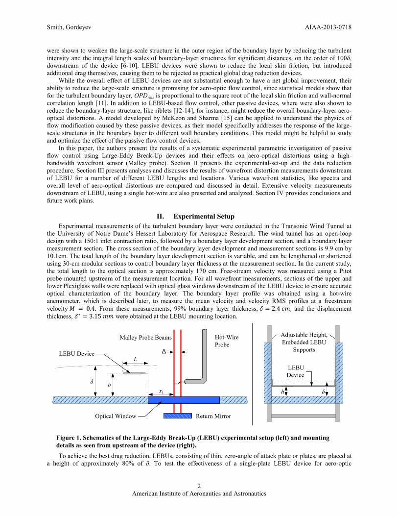
Figure 1. Schematics of the Large-Eddy Break-Up (LEBU) experimental setup (left) and mounting

details as seen from upstream of the device (right).

Smith, Gordeyev AIAA-2013-0718

3

American Institute of Aeronautics and Astronautics

mitigation in the turbulent boundary layer, several LEBU devices with different lengths, manufactured from 0.8 mm thick steel plate, were mounted to the wind tunnel side walls on two vertical sliding supports, as shown in Figure 1, which allowed for the continuous variation of the distance from the wall, h, that the LEBU was mounted at. The device spans the width of the test section, and as testing progresses, different LEBU heights (h) and lengths (𝐿) were tested, the full test matrix is shown in Table 1.

Table 1. LEBU Study Test Matrix and Data Types Obtained

Length (L) 19 mm 24 mm 38 mm

Height (h) 24 mm Malley Probe/Hot-Wire − Malley Probe 19 mm Malley Probe/Hot-Wire Malley Probe Malley Probe/Hot-Wire 15 mm Malley Probe/Hot-Wire Malley Probe Malley Probe/Hot-Wire 12 mm Malley Probe/Hot-Wire Malley Probe Malley Probe

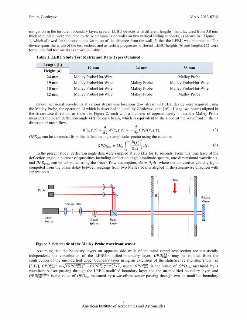
One-dimensional wavefronts at various streamwise locations downstream of LEBU device were acquired using

the Malley Probe, the operation of which is described in detail by Gordeyev, et al [16]. Using two beams aligned in the streamwise direction, as shown in Figure 2, each with a diameter of approximately 1 mm, the Malley Probe measures the beam deflection angle θ(t) for each beam, which is equivalent to the slope of the wavefront in the x-direction of mean flow,

𝜃(𝑥, 𝑧, 𝑡) =𝑑𝑑𝑥

𝑊(𝑥, 𝑧, 𝑡) = −𝑑𝑑𝑥

𝑂𝑃𝐷(𝑥, 𝑧, 𝑡). (2) OPDrms can be computed from the deflection angle amplitude spectra using the equation

𝑂𝑃𝐷𝑟𝑚𝑠2 = 2𝑈𝑐 ��𝜃�(𝑓)�2

(2𝜋𝑓)2∞

0𝑑𝑓. (3)

In the present study, deflection angle data were sampled at 200 kHz for 10 seconds. From this time trace of the deflection angle, a number of quantities including deflection angle amplitude spectra, one-dimensional wavefronts, and 𝑂𝑃𝐷𝑟𝑚𝑠 can be computed using the frozen-flow assumption, 𝑑𝑥 = 𝑈𝑐𝑑𝑡, where the convective velocity 𝑈𝑐 is computed from the phase delay between readings from two Malley beams aligned in the streamwise direction with separation Δ.

Assuming that the boundary layers on opposite side walls of the wind tunnel test section are statistically independent, the contribution of the LEBU-modified boundary layer, 𝑂𝑃𝐷𝑟𝑚𝑠𝐿𝐸𝐵𝑈

may be isolated from the contribution of the un-modified upper boundary layer using an extension of the statistical relationship shown in [3,17], 𝑂𝑃𝐷𝑟𝑚𝑠𝐿𝐸𝐵𝑈 = �(𝑂𝑃𝐷𝑟𝑚𝑠𝐷𝐵𝐿)2 − (𝑂𝑃𝐷𝑟𝑚𝑠

𝐵𝑎𝑠𝑒𝑙𝑖𝑛𝑒)2/2, where 𝑂𝑃𝐷𝑟𝑚𝑠𝐷𝐵𝐿 is the value of OPDrms measured by a wavefront sensor passing through the LEBU-modified boundary layer and the un-modified boundary layer, and 𝑂𝑃𝐷𝑟𝑚𝑠𝐵𝑎𝑠𝑒𝑙𝑖𝑛𝑒 is the value of OPDrms measured by a wavefront sensor passing through two un-modified boundary

Figure 2. Schematic of the Malley Probe wavefront sensor.

Laser Source Beam

Cube

Spatial Filter

Beam Splitter

PSDs TBL

Flow

Return Mirror

Smith, Gordeyev AIAA-2013-0718

4

American Institute of Aeronautics and Astronautics

layers in the control case. Similarly, it is also shown in [3] that deflection angle spectra of the LEBU-modified

boundary layer can be extracted in a similar manner, 𝜃�(𝑓)𝐿𝐸𝐵𝑈 = ��𝜃�(𝑓)𝐷𝐵𝐿�2 − �𝜃�(𝑓)𝐵𝑎𝑠𝑒𝑙𝑖𝑛𝑒�

2/2. In addition to wavefront measurements, hot-wire velocity profiles were obtained at several locations downstream of the LEBU devices with a single hot-wire mounted to a linear traverse and a commercial constant temperature anemometer. Velocity was measured for at 200 kHz for 5 seconds at each point in the profile, and the anemometer’s built-in low-pass filter was used with a cutoff frequency of 100 kHz. The hot-wire was calibrated in the freestream for Mach numbers ranging from M = 0.16 to 0.43. The freestream Mach number for each test was set at M = 0.4 to match the freestream velocity of the wavefront measurements.

III. Results

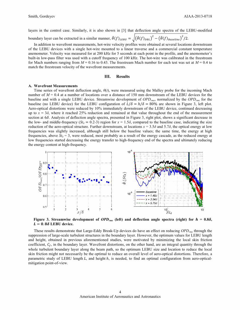
A. Wavefront Measurements Time series of wavefront deflection angle, θ(t), were measured using the Malley probe for the incoming Mach number of M = 0.4 at a number of locations over a distance of 150 mm downstream of the LEBU devices for the baseline and with a single LEBU device. Streamwise development of OPDrms, normalized by the OPDrms for the baseline (no LEBU device) for the LEBU configuration of 𝐿/𝛿 = ℎ/𝛿 = 80% are shown in Figure 3, left plot. Aero-optical distortions were reduced by 10% immediately downstream of the LEBU device, continued decreasing up to x = 3δ, where it reached 25% reduction and remained at that value throughout the end of the measurement section at 6𝛿. Analysis of deflection angle spectra, presented in Figure 3, right plot, shows a significant decrease in the low- and middle-frequency (Stδ = 0.2-3) region for x = 1.5δ, compared to the baseline case, indicating the size reduction of the aero-optical structure. Further downstream, at locations x = 3.5δ and 5.7δ, the optical energy at low frequencies was slightly increased, although still below the baseline values; the same time, the energy at high frequencies, above Stδ = 3, were reduced, most probably as a result of the energy cascade, as the reduced energy at low frequencies started decreasing the energy transfer to high-frequency end of the spectra and ultimately reducing the energy content at high-frequency.

Figure 3. Streamwise development of OPDrms (left) and deflection angle spectra (right) for 𝒉 = 0.8𝜹, 𝑳 = 𝟎.𝟖𝜹 LEBU device.

These results demonstrate that Large-Eddy Break-Up devices do have an effect on reducing OPDrms through the suppression of large-scale turbulent structures in the boundary layer. However, the optimum values for LEBU length and height, obtained in previous aforementioned studies, were motivated by minimizing the local skin friction coefficient, 𝐶𝑓, in the boundary layer. Wavefront distortions, on the other hand, are an integral quantity through the whole turbulent boundary layer along the beam path, so the optimum LEBU size and location to reduce the local skin friction might not necessarily be the optimal to reduce an overall level of aero-optical distortions. Therefore, a parametric study of LEBU length 𝐿, and height ℎ, is needed, to find an optimal configuration from aero-optical-mitigation point-of-view.

Smith, Gordeyev AIAA-2013-0718

5

American Institute of Aeronautics and Astronautics

1. LEBU Length Variation To investigate the effect of LEBU device streamwise length, L, aero-optical measurements were collected for

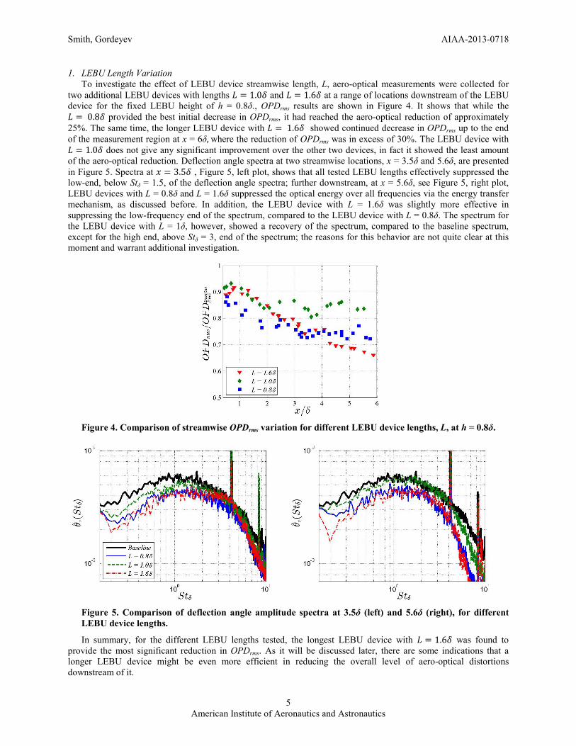
two additional LEBU devices with lengths 𝐿 = 1.0𝛿 and 𝐿 = 1.6𝛿 at a range of locations downstream of the LEBU device for the fixed LEBU height of h = 0.8δ., OPDrms results are shown in Figure 4. It shows that while the 𝐿 = 0.8𝛿 provided the best initial decrease in OPDrms, it had reached the aero-optical reduction of approximately 25%. The same time, the longer LEBU device with 𝐿 = 1.6𝛿 showed continued decrease in OPDrms up to the end of the measurement region at x = 6δ, where the reduction of OPDrms was in excess of 30%. The LEBU device with 𝐿 = 1.0𝛿 does not give any significant improvement over the other two devices, in fact it showed the least amount of the aero-optical reduction. Deflection angle spectra at two streamwise locations, x = 3.5δ and 5.6δ, are presented in Figure 5. Spectra at 𝑥 = 3.5𝛿 , Figure 5, left plot, shows that all tested LEBU lengths effectively suppressed the low-end, below Stδ = 1.5, of the deflection angle spectra; further downstream, at x = 5.6δ, see Figure 5, right plot, LEBU devices with L = 0.8δ and L = 1.6δ suppressed the optical energy over all frequencies via the energy transfer mechanism, as discussed before. In addition, the LEBU device with L = 1.6δ was slightly more effective in suppressing the low-frequency end of the spectrum, compared to the LEBU device with L = 0.8δ. The spectrum for the LEBU device with L = 1δ, however, showed a recovery of the spectrum, compared to the baseline spectrum, except for the high end, above Stδ = 3, end of the spectrum; the reasons for this behavior are not quite clear at this moment and warrant additional investigation.

Figure 4. Comparison of streamwise OPDrms variation for different LEBU device lengths, L, at h = 0.8δ.

Figure 5. Comparison of deflection angle amplitude spectra at 3.5δ (left) and 5.6δ (right), for different LEBU device lengths.

In summary, for the different LEBU lengths tested, the longest LEBU device with 𝐿 = 1.6𝛿 was found to provide the most significant reduction in OPDrms. As it will be discussed later, there are some indications that a longer LEBU device might be even more efficient in reducing the overall level of aero-optical distortions downstream of it.

Smith, Gordeyev AIAA-2013-0718

6

American Institute of Aeronautics and Astronautics

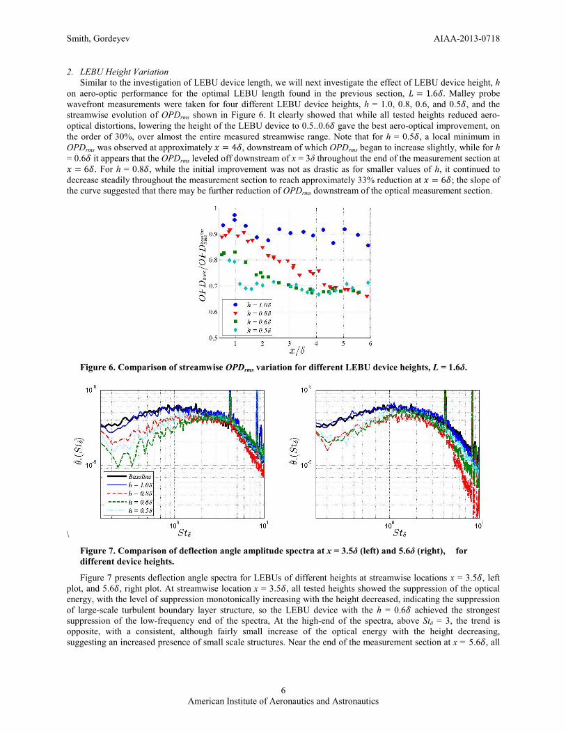
2. LEBU Height Variation Similar to the investigation of LEBU device length, we will next investigate the effect of LEBU device height, h on aero-optic performance for the optimal LEBU length found in the previous section, 𝐿 = 1.6𝛿. Malley probe wavefront measurements were taken for four different LEBU device heights, h = 1.0, 0.8, 0.6, and 0.5𝛿, and the streamwise evolution of OPDrms shown in Figure 6. It clearly showed that while all tested heights reduced aero-optical distortions, lowering the height of the LEBU device to 0.5..0.6𝛿 gave the best aero-optical improvement, on the order of 30%, over almost the entire measured streamwise range. Note that for h = 0.5𝛿, a local minimum in OPDrms was observed at approximately 𝑥 = 4𝛿, downstream of which OPDrms began to increase slightly, while for h = 0.6𝛿 it appears that the OPDrms leveled off downstream of x = 3δ throughout the end of the measurement section at 𝑥 = 6𝛿. For h = 0.8𝛿, while the initial improvement was not as drastic as for smaller values of h, it continued to decrease steadily throughout the measurement section to reach approximately 33% reduction at 𝑥 = 6𝛿; the slope of the curve suggested that there may be further reduction of OPDrms downstream of the optical measurement section.

Figure 6. Comparison of streamwise OPDrms variation for different LEBU device heights, L = 1.6δ.

\

Figure 7. Comparison of deflection angle amplitude spectra at x = 3.5δ (left) and 5.6δ (right), for different device heights.

Figure 7 presents deflection angle spectra for LEBUs of different heights at streamwise locations x = 3.5𝛿, left plot, and 5.6𝛿, right plot. At streamwise location x = 3.5𝛿, all tested heights showed the suppression of the optical energy, with the level of suppression monotonically increasing with the height decreased, indicating the suppression of large-scale turbulent boundary layer structure, so the LEBU device with the h = 0.6𝛿 achieved the strongest suppression of the low-frequency end of the spectra, At the high-end of the spectra, above Stδ = 3, the trend is opposite, with a consistent, although fairly small increase of the optical energy with the height decreasing, suggesting an increased presence of small scale structures. Near the end of the measurement section at x = 5.6𝛿, all

Smith, Gordeyev AIAA-2013-0718

7

American Institute of Aeronautics and Astronautics

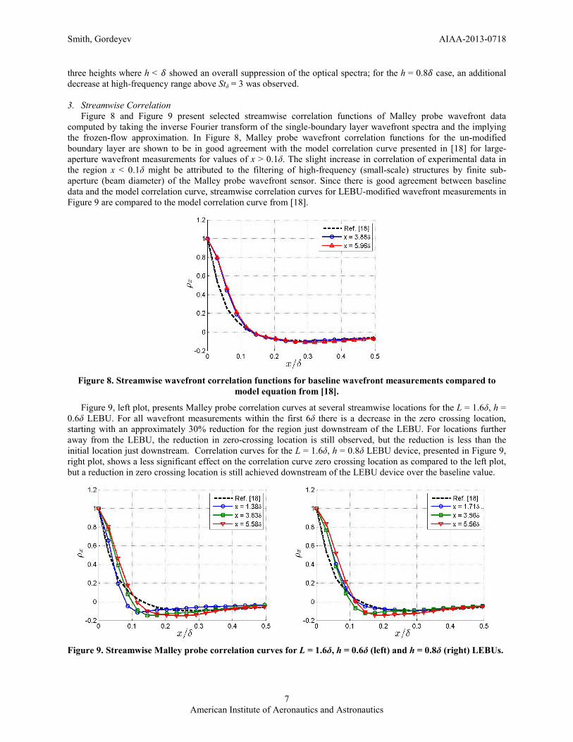
three heights where h < 𝛿 showed an overall suppression of the optical spectra; for the h = 0.8𝛿 case, an additional decrease at high-frequency range above Stδ = 3 was observed. 3. Streamwise Correlation Figure 8 and Figure 9 present selected streamwise correlation functions of Malley probe wavefront data computed by taking the inverse Fourier transform of the single-boundary layer wavefront spectra and the implying the frozen-flow approximation. In Figure 8, Malley probe wavefront correlation functions for the un-modified boundary layer are shown to be in good agreement with the model correlation curve presented in [18] for large-aperture wavefront measurements for values of x > 0.1δ. The slight increase in correlation of experimental data in the region x < 0.1δ might be attributed to the filtering of high-frequency (small-scale) structures by finite sub-aperture (beam diameter) of the Malley probe wavefront sensor. Since there is good agreement between baseline data and the model correlation curve, streamwise correlation curves for LEBU-modified wavefront measurements in Figure 9 are compared to the model correlation curve from [18].

Figure 8. Streamwise wavefront correlation functions for baseline wavefront measurements compared to

model equation from [18].

Figure 9, left plot, presents Malley probe correlation curves at several streamwise locations for the L = 1.6δ, h = 0.6δ LEBU. For all wavefront measurements within the first 6δ there is a decrease in the zero crossing location, starting with an approximately 30% reduction for the region just downstream of the LEBU. For locations further away from the LEBU, the reduction in zero-crossing location is still observed, but the reduction is less than the initial location just downstream. Correlation curves for the L = 1.6δ, h = 0.8δ LEBU device, presented in Figure 9, right plot, shows a less significant effect on the correlation curve zero crossing location as compared to the left plot, but a reduction in zero crossing location is still achieved downstream of the LEBU device over the baseline value.

Figure 9. Streamwise Malley probe correlation curves for L = 1.6δ, h = 0.6δ (left) and h = 0.8δ (right) LEBUs.

Smith, Gordeyev AIAA-2013-0718

8

American Institute of Aeronautics and Astronautics

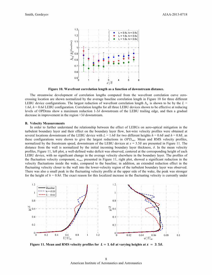
Figure 10. Wavefront correlation length as a function of downstream distance.

The streamwise development of correlation lengths computed from the wavefront correlation curve zero-crossing location are shown normalized by the average baseline correlation length in Figure 10 for three different LEBU device configurations. The largest reduction of wavefront correlation length Λ𝑥 is shown to be by the L = 1.6δ, h = 0.6δ LEBU configuration. Correlation lengths for all three LEBU devices shown to be effective at reducing levels of OPDrms show a maximum reduction 1-3δ downstream of the LEBU trailing edge, and then a gradual decrease in improvement in the region >3δ downstream.

B. Velocity Measurements In order to further understand the relationship between the effect of LEBUs on aero-optical mitigation in the turbulent boundary layer and their effect on the boundary layer flow, hot-wire velocity profiles were obtained at several locations downstream of the LEBU device with L = 1.6𝛿 for two different heights h = 0.6𝛿 and h = 0.8𝛿, as these configurations were shown to give the largest reductions in OPDrms. Mean and RMS velocity profiles, normalized by the freestream speed, downstream of the LEBU devices at x = 3.5𝛿 are presented in Figure 11. The distance from the wall is normalized by the initial incoming boundary layer thickness, δ. In the mean velocity profiles, Figure 11, left plot, a well-defined wake deficit was observed, centered at the corresponding height of each LEBU device, with no significant change in the average velocity elsewhere in the boundary layer. The profiles of the fluctuation velocity component, urms, presented in Figure 11, right plot, showed a significant reduction in the velocity fluctuations inside the wake, compared to the baseline; in addition, an extended reduction effect in the fluctuating velocity closer to the wall into the lower-velocity region of the turbulent boundary layer was observed. There was also a small peak in the fluctuating velocity profile at the upper side of the wake, the peak was stronger for the height of h = 0.8δ. The exact reason for this localized increase in the fluctuating velocity is currently under

Figure 11. Mean and RMS velocity profiles for 𝑳 = 𝟏.𝟔𝜹 at varying heights at 𝒙 = 𝟑.𝟓𝜹.

Smith, Gordeyev AIAA-2013-0718

9

American Institute of Aeronautics and Astronautics

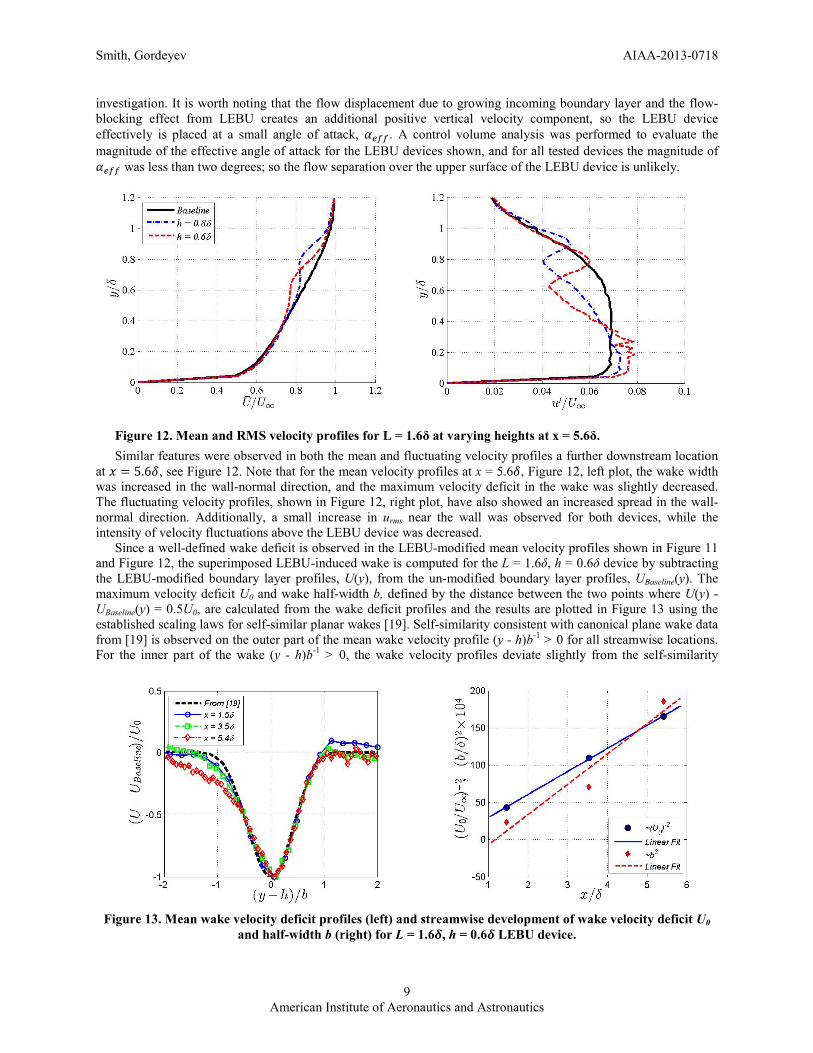
investigation. It is worth noting that the flow displacement due to growing incoming boundary layer and the flow-blocking effect from LEBU creates an additional positive vertical velocity component, so the LEBU device effectively is placed at a small angle of attack, 𝛼𝑒𝑓𝑓 . A control volume analysis was performed to evaluate the magnitude of the effective angle of attack for the LEBU devices shown, and for all tested devices the magnitude of 𝛼𝑒𝑓𝑓 was less than two degrees; so the flow separation over the upper surface of the LEBU device is unlikely.

Similar features were observed in both the mean and fluctuating velocity profiles a further downstream location at 𝑥 = 5.6𝛿, see Figure 12. Note that for the mean velocity profiles at x = 5.6𝛿, Figure 12, left plot, the wake width was increased in the wall-normal direction, and the maximum velocity deficit in the wake was slightly decreased. The fluctuating velocity profiles, shown in Figure 12, right plot, have also showed an increased spread in the wall-normal direction. Additionally, a small increase in urms near the wall was observed for both devices, while the intensity of velocity fluctuations above the LEBU device was decreased. Since a well-defined wake deficit is observed in the LEBU-modified mean velocity profiles shown in Figure 11 and Figure 12, the superimposed LEBU-induced wake is computed for the L = 1.6δ, h = 0.6δ device by subtracting the LEBU-modified boundary layer profiles, U(y), from the un-modified boundary layer profiles, UBaseline(y). The maximum velocity deficit U0 and wake half-width b, defined by the distance between the two points where U(y) - UBaseline(y) = 0.5U0, are calculated from the wake deficit profiles and the results are plotted in Figure 13 using the established scaling laws for self-similar planar wakes [19]. Self-similarity consistent with canonical plane wake data from [19] is observed on the outer part of the mean wake velocity profile (y - h)b-1 > 0 for all streamwise locations. For the inner part of the wake (y - h)b-1 > 0, the wake velocity profiles deviate slightly from the self-similarity

Figure 12. Mean and RMS velocity profiles for L = 1.6δ at varying heights at x = 5.6δ.

Figure 13. Mean wake velocity deficit profiles (left) and streamwise development of wake velocity deficit U0

and half-width b (right) for L = 1.6𝜹, h = 0.6𝜹 LEBU device.

Smith, Gordeyev AIAA-2013-0718

10

American Institute of Aeronautics and Astronautics

scaling as streamwise distance downstream of the LEBU device increases. Planar wake self-similar behavior was also observed in the scaling of U0 and b as a function of streamwise location in Figure 13, right plot, using the respective linear growth scaling where x ~ b2, and x ~ U0

-2. The growth rate 𝛼 = 1Θ𝑑𝑏2

𝑑𝑥 , where Θ is the wake

momentum thickness, was found to be approximately 0.15 for the LEBU wake velocity profiles, which is less than the range of published growth rate values of 0.29-0.41 for self-similar planar wakes [19]. Fluctuating velocity measurements, however, were found to not scale as a self-similar planar wake, due to the large reduction in urms below the LEBU device shown in Figure 11 and Figure 12. One possible reason for this observed behavior is that because the LEBU device induces a wake in a sheared mean flow, it reduces the local velocity gradient below the LEBU device and increases the velocity gradient above it, see Figure 11, right. This local mean velocity modification results in either a reduction or an increase in the turbulent fluctuating velocity component downstream of the LEBU device, as the dominant turbulence production term, )/('' dydUvu , is proportional to local the mean velocity gradient. In [5,11] it was shown that the main mechanism for unsteady density fluctuations in turbulent boundary layers, which is ultimately responsible for aero-optical distortions, is due to an adiabatic heating/cooling, so-called Strong Reynolds Analogy, )(')(~)(' yuyUyρ . Substituting it into the linking equation [20], it was shown that OPDrms for canonical boundary layer can be correctly predicted from the velocity field as follows [3]

𝑂𝑃𝐷𝑟𝑚𝑠 = √2𝐾𝐺𝐷𝜌∞𝛿𝑀2(𝛾 − 1) �� �𝑟2 �𝑈�(𝑦)𝑢𝑟𝑚𝑠(𝑦)

𝑈∞2�2 Λ𝜌(𝑦)

𝛿� 𝑑 �

𝑦𝛿�

∞

0�

12

,

(4)

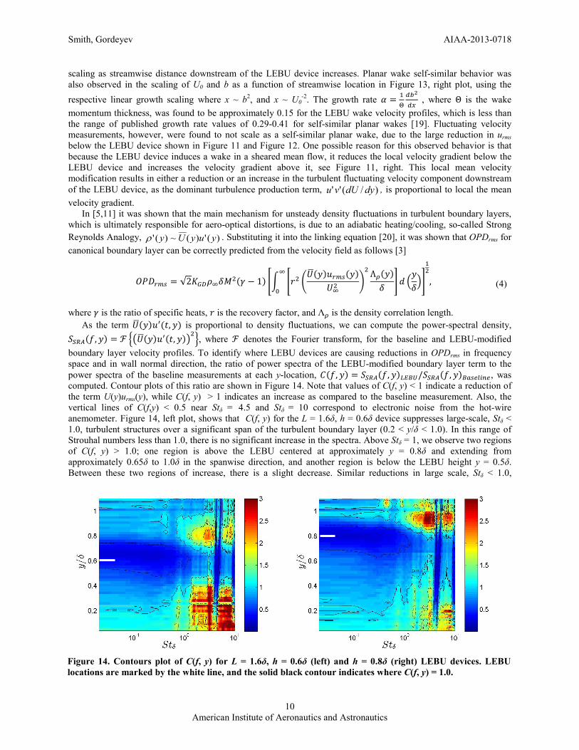
where 𝛾 is the ratio of specific heats, 𝑟 is the recovery factor, and Λ𝜌 is the density correlation length. As the term 𝑈�(𝑦)𝑢′(𝑡,𝑦) is proportional to density fluctuations, we can compute the power-spectral density, 𝑆𝑆𝑅𝐴(𝑓,𝑦) = ℱ ��𝑈�(𝑦)𝑢′(𝑡,𝑦)�2�, where ℱ denotes the Fourier transform, for the baseline and LEBU-modified boundary layer velocity profiles. To identify where LEBU devices are causing reductions in OPDrms in frequency space and in wall normal direction, the ratio of power spectra of the LEBU-modified boundary layer term to the power spectra of the baseline measurements at each y-location, 𝐶(𝑓,𝑦) = 𝑆𝑆𝑅𝐴(𝑓,𝑦)𝐿𝐸𝐵𝑈/𝑆𝑆𝑅𝐴(𝑓,𝑦)𝐵𝑎𝑠𝑒𝑙𝑖𝑛𝑒, was computed. Contour plots of this ratio are shown in Figure 14. Note that values of C(f, y) < 1 indicate a reduction of the term U(y)urms(y), while C(f, y) > 1 indicates an increase as compared to the baseline measurement. Also, the vertical lines of C(f,y) < 0.5 near Stδ = 4.5 and Stδ = 10 correspond to electronic noise from the hot-wire anemometer. Figure 14, left plot, shows that C(f, y) for the L = 1.6δ, h = 0.6δ device suppresses large-scale, Stδ < 1.0, turbulent structures over a significant span of the turbulent boundary layer (0.2 < y/δ < 1.0). In this range of Strouhal numbers less than 1.0, there is no significant increase in the spectra. Above Stδ = 1, we observe two regions of C(f, y) > 1.0; one region is above the LEBU centered at approximately y = 0.8δ and extending from approximately 0.65δ to 1.0δ in the spanwise direction, and another region is below the LEBU height y = 0.5δ. Between these two regions of increase, there is a slight decrease. Similar reductions in large scale, Stδ < 1.0,

Figure 14. Contours plot of C(f, y) for L = 1.6δ, h = 0.6δ (left) and h = 0.8δ (right) LEBU devices. LEBU locations are marked by the white line, and the solid black contour indicates where C(f, y) = 1.0.

Smith, Gordeyev AIAA-2013-0718

11

American Institute of Aeronautics and Astronautics

turbulent structures is observed in Figure 14, right plot, for the L = 1.6δ, h = 0.8δ LEBU device. Above Stδ = 1, we also observe two regions of C(f, y) > 1.0; one is above the LEBU centered at approximately y = 0.9δ and extending from approximately 0.8δ to 1.1δ in the spanwise direction, and another is below the LEBU height y = 0.6δ. Note that, compared to the h = 0.6δ device, the region of increased C(f, y) above Stδ = 1, y = 0.8δ shows an increase in energy that is approximately 1.5 times greater. For the region above Stδ = 1 and near the wall, however, the increase in C(f, y), is less significant that the increase shown for the h = 0.6δ LEBU.

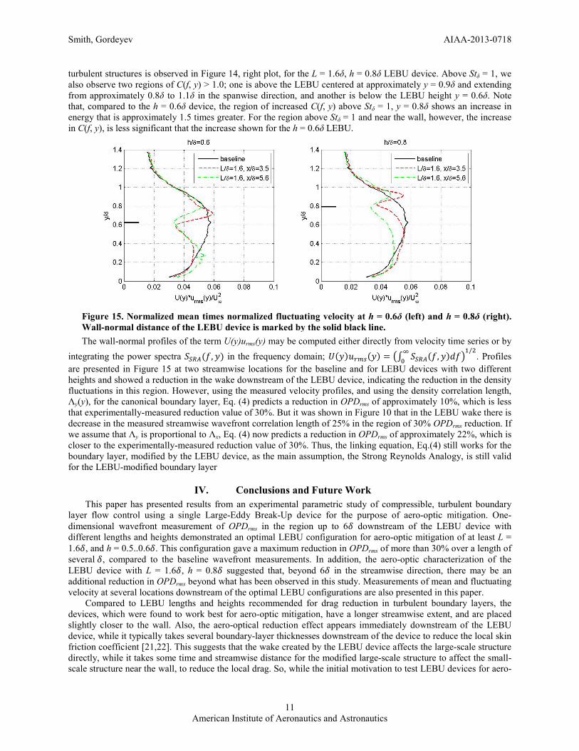
The wall-normal profiles of the term U(y)urms(y) may be computed either directly from velocity time series or by integrating the power spectra 𝑆𝑆𝑅𝐴(𝑓,𝑦) in the frequency domain; 𝑈(𝑦)𝑢𝑟𝑚𝑠(𝑦) = �∫ 𝑆𝑆𝑅𝐴(𝑓,𝑦)𝑑𝑓∞

0 �1/2

. Profiles are presented in Figure 15 at two streamwise locations for the baseline and for LEBU devices with two different heights and showed a reduction in the wake downstream of the LEBU device, indicating the reduction in the density fluctuations in this region. However, using the measured velocity profiles, and using the density correlation length, Λy(y), for the canonical boundary layer, Eq. (4) predicts a reduction in OPDrms of approximately 10%, which is less that experimentally-measured reduction value of 30%. But it was shown in Figure 10 that in the LEBU wake there is decrease in the measured streamwise wavefront correlation length of 25% in the region of 30% OPDrms reduction. If we assume that Λy is proportional to Λx, Eq. (4) now predicts a reduction in OPDrms of approximately 22%, which is closer to the experimentally-measured reduction value of 30%. Thus, the linking equation, Eq.(4) still works for the boundary layer, modified by the LEBU device, as the main assumption, the Strong Reynolds Analogy, is still valid for the LEBU-modified boundary layer

IV. Conclusions and Future Work This paper has presented results from an experimental parametric study of compressible, turbulent boundary layer flow control using a single Large-Eddy Break-Up device for the purpose of aero-optic mitigation. One-dimensional wavefront measurement of OPDrms in the region up to 6𝛿 downstream of the LEBU device with different lengths and heights demonstrated an optimal LEBU configuration for aero-optic mitigation of at least L = 1.6𝛿, and h = 0.5..0.6𝛿. This configuration gave a maximum reduction in OPDrms of more than 30% over a length of several 𝛿, compared to the baseline wavefront measurements. In addition, the aero-optic characterization of the LEBU device with L = 1.6𝛿, h = 0.8𝛿 suggested that, beyond 6𝛿 in the streamwise direction, there may be an additional reduction in OPDrms beyond what has been observed in this study. Measurements of mean and fluctuating velocity at several locations downstream of the optimal LEBU configurations are also presented in this paper. Compared to LEBU lengths and heights recommended for drag reduction in turbulent boundary layers, the devices, which were found to work best for aero-optic mitigation, have a longer streamwise extent, and are placed slightly closer to the wall. Also, the aero-optical reduction effect appears immediately downstream of the LEBU device, while it typically takes several boundary-layer thicknesses downstream of the device to reduce the local skin friction coefficient [21,22]. This suggests that the wake created by the LEBU device affects the large-scale structure directly, while it takes some time and streamwise distance for the modified large-scale structure to affect the small-scale structure near the wall, to reduce the local drag. So, while the initial motivation to test LEBU devices for aero-

Figure 15. Normalized mean times normalized fluctuating velocity at h = 0.6δ (left) and h = 0.8δ (right).

Wall-normal distance of the LEBU device is marked by the solid black line.

Smith, Gordeyev AIAA-2013-0718

12

American Institute of Aeronautics and Astronautics

optical mitigation was the link between OPDrms and Cf, OPDrms ~ (Cf)1/2, this relation was shown to work only in the canonical turbulent boundary layer, where the global quantity OPDrms and the near-wall local Cf are interconnected, as the large-scale and the near-wall structures are an equilibrium state. The LEBU device directly modifies the outer-region of the boundary layer, thus disrupting this global equilibrium. Results from this experiment showed that one way to directly modify large-scale turbulent structures is to decrease the local mean velocity by introducing a higher turbulent dissipation without significantly increasing the turbulent velocity fluctuations. Therefore, it is of interest to study a wider class of passive boundary layer flow control devices such as thin pin fences and fine screens, and their effect on boundary layer aero-optic mitigation; note that these devices were already shown to reduce aero-optical distortions of the separated shear layer [23] and to eliminate the local shocks over turrets at transonic speeds by slowing the local flow [24]. Future work on this topic includes extending aero-optical characterization of the LEBU wake up to and beyond 10𝛿 downstream, and further investigating the effects of different LEBUs lengths and heights on the streamwise extent and overall levels of aero-optic mitigation in the turbulent boundary layer. In addition, studies of multiple-LEBU devices and their effects on aero-optical distortions are needed. Additional velocity characterizations will be performed with hot-wires and x-wires, along with PIV and simultaneous aero-optical measurements in order to better understand the effect of LEBUs on unsteady density field in the turbulent boundary layers, as well as the spanwise density correlation length.

Acknowledgments

This work is supported by the Air Force Office of Scientific Research, Grant number FA9550-12-1-0060. The U.S. Government is authorized to reproduce and distribute reprints for governmental purposes notwithstanding any copyright notation thereon.

References

[1] Jumper, E.J., and Fitzgerald, E.J., 2001, “Recent Advances in Aero-Optics,” Progress in Aerospace Sciences, 37, 299-339.

[2] M. Wang, A.Mani and S. Gordeyev,”Physics and Computation of Aero-Optics”, Annual Review of Fluid Mechanics, Vol. 44, pp. 299-321, 2012.

[3] Cress, J. (2010) Optical Aberrations Cause by Coherent Structures in a Subsonic, Compressible, Turbulent Boundary Layer, PhD thesis, University of Notre Dame.

[4] Cress, J., Gordeyev, S., and Jumper E.J., “Aero-Optical Measurements in a Heated, Subsonic, Turbulent Boundary Layer,” 48th AIAA Aerospace Sciences Meeting Including the New Horizons Forum and Aerospace Exposition, AIAA-2010-434, Orlando, FL, January 2010.

[5] Wang, K. and Wang, M., “Aero-optics of subsonic turbulent boundary layers,” Journal of Fluid Mechanics, Vol. 696, pp. 122-151, 2012.

[6] Corke TC, Guezennec YG, Nagib HM. “Modification in drag of turbulent boundary layers resulting from manipulation of large-scale structures.” In Proc. Viscous Drag Reduction Symp., Dallas. AIAA Prog. Astro. Aero. 72, 128-143. (1979)

[7] Plesniak MW, Naqib HM. “Net drag reduction in turbulent boundary layers resulting from optimized manipulation.” AIAA-85-0518. (1985)

[8] Bandyopadhyay, P.R. “Review - Mean flow in turbulent boundary layers disturbed to alter skin friction.” Trans. ASME J . Fluids Engng 108, 127-140. (1986)

[9] Westphal, R.V., “Skin friction and Reynolds Stress measurements for a turbulent boundary layer following manipulation using flat plates.” AIAA, Aerospace Sciences Meeting, 24th, Reno, NV, Jan. 6-9, 1986 (AIAA-86-0283)

[10] Bonnet J.P., Delville J., Lemay J., “Study of LEBUs modified turbulent boundary layer by use of passive temperature contamination.” In Proc. Turbulent Drag Reduction by Passive Means, vol. 1, pp. 45-68. R. Aero. Soc. (1987)

[11] Gordeyev, S., Jumper, E.J., and Hayden, T., "Aero-Optics of Supersonic Boundary Layers," AIAA Journal, 50(3), 682-690, 2012.

[12] Walsh, M. J., “Riblets,” Viscous Drag Reduction in Boundary Layers, eds. D. M. Bushnell and J. N. Heffner, pages 203–261. AIAA, Washington, D.C., 1990.

Smith, Gordeyev AIAA-2013-0718

13

American Institute of Aeronautics and Astronautics

[13] Walsh, M.J. and Anders, J.B., 1989. Riblet/LEBU research at NASA Langley. Applied Scientific Research 46: 255-262.

[14] L. Sirovich and S. Karlsson. 1997. Turbulent drag reduction by passive mechanisms. Nature, 388(21):753–755. [15] McKeon BJ & Sharma A. 2010 A critical layer framework for turbulent pipe flow. J. Fluid Mech., 658, 336-

382. [16] Gordeyev, S., Duffin, D., and Jumper, E.J., “Aero-Optical Measurements Using Malley Probe and High-

Bandwidth 2-D Wavefront Sensors,” International Conference on Advanced Optical Diagnostics in Fluids, Solids, and Combustion, Tokyo, Japan, Dec. 2004.

[17] Wittich, D. J., Gordeyev, S., and Jumper, E. J., “Revised scaling of optical distortions caused by compressible, subsonic turbulent boundary layers.” 38th AIAA Plasmadynamics and Lasers Conference, AIAA-2007-4009, Miami, FL, June 2007.

[18] Smith, A.E., Gordeyev, S., and Jumper, E.J., “Aperture Effects on Aero-Optical Distortions Caused by Subsonic Boundary Layers,” 43rd AIAA Plasmadynamics and Lasers Conference, 25 - 28 June 2012, New Orleans, LA, AIAA Paper 2012-2986

[19] Moser, R.D., Rogers, M.M., and Ewing, D.W., “Self-similarity of time-evolving plane wakes,” J. Fluid Mech., 367, 255-289, 1998.

[20] Sutton, G.W., “Effect of turbulent fluctuations in an optically active fluid medium.” AIAA Journal, 7(9): 1737-1743, Sept. 1969.

[21] Savill, A.M., and Mumford, J.C., “Manipulation of turbulent boundary layers by outer-layer devices: skin-friction and flow-visualization results,” J. Fluid Mech., 191, 389-418, 1988.

[22] Hefner, J.N., Weinstein, L.M., and Bushnell, D.M., “Large-Eddy Breakup Scheme for Turbulent Viscous Drag Reduction,” Proc. Viscous Drag Reduction Symp., Dallas. AIAA Prog. Astro. Aero. 72, 110-127. (1979)

[23] Gordeyev, S., Cress, J., Smith, A.E., and Jumper, E., “Improvement in Optical Environment over Turrets with Flat Window Using Passive Flow Control,” 41th AIAA Plasmadynamics and Lasers Conference, Chicago, IL, Jun. 28 – Jul. 1, 2010, AIAA Paper 2010-4492.

[24] Gordeyev, S., Burns, R., Jumper, E.J., Gogineni, S., and Wittich, D.J., “Aero-Optical Mitigation of Shocks Around Turrets at Transonic Speeds Using Passive Flow Control,” 51st AIAA Aerospace Sciences Meeting, Grapevine, TX, 7 - 10 January 2013, AIAA Paper 2013-0717.