Embed Size (px)
Citation preview

POLITECNICO DI MILANO
Scuola di Ingegneria Industriale e dell’Informazione
Corso di Laurea Magistrale in
Ingegneria Energetica
Evaluation of ORC processes and their implementation
in solar thermal DSG plants
Relatore: Prof. Paolo SILVA
Co-relatore: M.Sc. Heiko SCHENK
Tesi di Laurea di:
Dalma DEGLI ESPOSTI Matr. 783376
Anno Accademico 2012 - 2013


i
Acknowledgements
Innanzitutto, vorrei ringraziare il Professor Paolo Silva per la sua infinita disponibilità
e per avermi dato la possibilità di sviluppare questa tesi in Germania.
Un sincero ringraziamento va in particolare ad Andrea Giostri, che ha pazientemente
messo a disposizione la sua conoscenza continuando a seguire il mio lavoro anche da
lontano. Lo ringrazio per il supporto iniziale in quel di Stoccarda. Il primo mese in
ufficio è stato come sentirsi a casa.
Besonderer Dank geht an meinen Betreuer M.Sc. Heiko Schenk vom DLR Stuttgart,
der diese Masterarbeit ermöglicht hat. Ich bedanke mich bei ihm für die
wöchentlichen jour fixe Termine, in denen er mir ausführlich zu allen Fragen und
Problemstellungen mit Rat und Tat zur Seite stand. Weiterhin möchte ich mich bei
allen Mitarbeitern des Instituts für Solarforschung am Standort Stuttgart für die
angenehme und freundschaftliche Zusammenarbeit bedanken.
Il ringraziamento più grande va però a Mamma e Papà, per aver sempre creduto in me
e avermi supportato in ogni momento e in ogni mia scelta da sempre. Un
ringraziamento speciale va alla mia Nonna, per esserci sempre stata in ogni
occasione.
Grazie alla mia Sis e a tutti gli Amici di Brixen, Milano e Torino che nonostante la
lontananza sono sempre stati presenti, dimostrando quanto il nostro legame sia forte.
Inoltre, un doveroso ringraziamento va al mio collega di fiducia e ai “piccoli ing.”,
che oltre ad esser stati miei compagni d’avventura al Politecnico, si sono rivelati degli
ottimi amici.
Un grazie speciale va poi alla mia “Stuttgart-Family”, che ha contribuito a rendere
piacevoli e divertenti questi mesi di permanenza all’estero.
Infine un pensiero va a tutte le persone che in questi anni hanno condiviso con me
parte di questo percorso tra Milano, Monaco e Stoccarda. A chi c’era, c’è e c’è
sempre stato. Grazie!

ii

iii
Index
Index of figures ................................................................................................. vii
Index of tables ................................................................................................... xii
Abstract ............................................................................................................ xiv
Sommario ......................................................................................................... xvi
Introduction ................................................................................................... xviii Background ..................................................................................................... xviii Objectives .......................................................................................................... xix
1 Concentrated solar power plants (CSP) .................................................... 1 1.1 State-of-the-art of concentrated solar power systems .............................. 3
1.1.1 Parabolic trough ............................................................................... 4 1.1.2 Linear Fresnel collectors .................................................................. 6
1.1.3 Solar towers ...................................................................................... 7 1.1.4 Parabolic dish ................................................................................... 8
1.2 Overview of existing parabolic trough power plants ............................... 9 1.2.1 Parabolic trough plants with thermal oil .......................................... 9 1.2.2 Parabolic trough plants with molten salt ........................................ 11
1.2.3 Parabolic trough plants with DSG .................................................. 12
1.2.4 Parabolic trough plants with ORC ................................................. 15
2 Organic Rankine Cycle Background ....................................................... 17 2.1 Typical configuration............................................................................. 18
2.2 Organic working fluids .......................................................................... 20 2.2.1 Characteristics of the organic working fluids ................................ 20
2.2.2 Classification of fluids based on the T-s diagram .......................... 21 2.2.3 Mixtures ......................................................................................... 23
2.3 Comparison with the steam Rankine cycle ............................................ 24
2.3.1 Thermodynamic and physical differences...................................... 24 2.3.2 Power and temperature range ......................................................... 26
2.3.3 Turbine design ................................................................................ 27 2.4 ORC applications ................................................................................... 28
3 The choice of the organic working fluid .................................................. 31 3.1 Selection criteria .................................................................................... 31 3.2 Screening of available fluids ................................................................. 33
3.2.1 ORC fluids classified by application .............................................. 37 3.2.2 ORC fluids used by manufacturers ................................................ 40
3.3 Suitable organic fluids for DSG ............................................................ 41

iv
3.3.1 LT fluids: R245fa, SES36 .............................................................. 42 3.3.2 HT fluids: Siloxanes ....................................................................... 44
4 ORC processes analysis ............................................................................. 47 4.1 Regenerative cycles ................................................................................ 48 4.2 Basic cycle analysis model ..................................................................... 50
4.3 Thermodynamic optimization of siloxanes ............................................ 53 4.3.1 Condensing pressure ....................................................................... 54 4.3.2 Maximum temperature.................................................................... 55 4.3.3 Volume flow ratio ........................................................................... 56
4.4 Thermodynamic analysis ....................................................................... 59
4.5 Integration of storage: a thermodynamic evaluation .............................. 62
5 Solar thermal ORC power plant Modelization ....................................... 67 5.1 Preliminary Sizing .................................................................................. 67
5.2 EBSILON®
Professional ......................................................................... 69 5.3 Solar field ............................................................................................... 72
5.3.1 The sun............................................................................................ 72 5.3.2 Parabolic trough collector ............................................................... 73
5.3.3 Layout ............................................................................................. 80 5.4 Thermal storage system .......................................................................... 83
5.5 Power block ............................................................................................ 86 5.5.1 ORC Turbine .................................................................................. 87 5.5.2 Regenerator ..................................................................................... 89
5.5.3 Condenser and cooling system ....................................................... 90
5.5.4 Pump ............................................................................................... 92 5.6 Reference systems .................................................................................. 93 5.7 Simulation layouts .................................................................................. 93
5.8 Plant operation management .................................................................. 96 5.8.1 Start and stand-by operation mode ................................................. 96
5.8.2 Solar operation and charging mode ................................................ 97 5.8.3 Defocus mode ................................................................................. 97
5.8.4 Solar operation and discharging mode ........................................... 98 5.8.5 Storage-only operation mode .......................................................... 99
6 Evaluation of simulation data ................................................................. 101 6.1 Design results ....................................................................................... 103 6.2 Off-design analysis ............................................................................... 104
6.2.1 Case-study: supercritical cycle configuration ............................... 105 6.2.2 Case-study: saturated cycle configuration .................................... 112
6.3 Simulation of typical days .................................................................... 117 6.3.1 Simulation of a summer day ......................................................... 117 6.3.2 Simulation of a winter day ............................................................ 119 6.3.3 Simulation of a mid-season day .................................................... 121

v
Conclusions ..................................................................................................... 125
Appendix .............................................................................................................. I
References ........................................................................................................... V

vi

vii
Index of figures
Figure 1.1: Global map of annual DNI [© METEOTEST; based on
www.meteonorm.com] .................................................................... 1 Figure 1.2: Main types of CSP: (a) Parabolic trough collectors; (b) Linear
Fresnel collectors; (c) Solar Tower; (d) Solar dish (DLR) .............. 3 Figure 1.3: SEGS solar power plants III-VII at Mojave Desert, California ...... 4
Figure 1.4: Schematic diagram of parabolic trough collectors and a
detailed HCE (Flabeg Solar International) ...................................... 5
Figure 1.5: Linear Fresnel reflector with one absorber (DLR/Novatec
Solar) ............................................................................................... 6 Figure 1.6: Solar tower PS10 in Spain [12] ....................................................... 7 Figure 1.7: Parabolic dish (DLR)....................................................................... 8
Figure 1.8: Schematic configuration of a parabolic trough power plant
with oil as HTF (Flabeg Solar International) ................................ 10 Figure 1.9: Schematic configuration of a parabolic trough power plant
with molten salt as HTF (DLR) ..................................................... 11 Figure 1.10: Schematic configuration of a parabolic trough plant with DSG
(DLR) ............................................................................................ 12 Figure 1.11: Representation of the stratified and anular flow in the
evaporation zone [25] .................................................................... 13 Figure 1.12: Three basic DSG processes (DISS) ............................................... 14
Figure 1.13: Schematic configuration of a parabolic trough power plant
with ORC [5] ................................................................................. 15 Figure 2.1: T-s diagram for the ideal/real ORC cycle using isopentane as
working fluid ................................................................................. 18 Figure 2.2: Component diagrams of a basic ORC (left) and a regenerative
ORC (right) [35] ............................................................................ 19 Figure 2.3: T-s diagram of water and various ORC fluids [36] ....................... 21 Figure 2.4: Saturation curves of a dry, wet and isentropic fluid [37] .............. 22
Figure 2.5: Effect of molecule size on the slope .............................................. 22 Figure 2.6: Qualitative representation of an isobaric phase change for a
two-components mixture in the T-s and T-x (x = mole
fraction) diagrams [39] .................................................................. 23
Figure 2.7: Rankine cycle for water (a) and for dry organic fluids (b) ............ 25 Figure 2.8: Field of applications in a temperature versus power diagram
[43] ................................................................................................ 26 Figure 2.9: Axial and radial turbine stages [45] .............................................. 27

viii
Figure 2.10: ORC market evolution and share of each application in terms
of number of units adapted from [35] ........................................... 28 Figure 3.1: Critical temperature as function of the critical pressure of the
screened organic fluids ................................................................. 35 Figure 3.2: Graphical overview of the ODP and GWP indexes of some
organic fluids ................................................................................ 35 Figure 3.3: Critical temperature and pressure of the selected ORC fluid
families .......................................................................................... 41 Figure 3.4: T-s diagram of R245fa .................................................................. 42 Figure 3.5: T-s diagram of Solkatherm® SES 36 ........................................... 43
Figure 3.6: T-s diagram and proven thermal stability limit of linear
siloxanes [74] ................................................................................ 44 Figure 3.7: T-s diagram and proven thermal stability limit of cyclic
siloxanes [74] ................................................................................ 45 Figure 4.1: Flow chart of the performed analysis ........................................... 47 Figure 4.2: Representative T-s diagram of a subcritical saturated cycle ......... 48 Figure 4.3: Representative T-s diagram of a subcritical superheated cycle .... 49
Figure 4.4: Representative T-s diagram of a supercritical cycle ..................... 50 Figure 4.5: Schematic representation of ORC components and working
fluid state points ............................................................................ 51 Figure 4.6: Evaluation of condensing pressure and corresponding
temperature for siloxanes .............................................................. 55
Figure 4.7: Turbine isentropic volume flow ratio for an isentropic
expansion as a function of condensing temperature for a
maximum cycle temperature of 280°C ......................................... 58 Figure 4.8: Turbine size parameter as a function of condesing temperature
for a maximum cycle temperature of 280°C ................................. 58 Figure 4.9: Specific speed as a function of the condensing temperature for
a maximum cycle temperature of 280°C ...................................... 58 Figure 4.10: Specific net work as a function of condensing temperature in
both configurations for a maximum cycle temperature of
280°C ............................................................................................ 59 Figure 4.11: Cycle efficiency as a function of condensing temperature in
both configurations for a maximum cycle temperature of
280°C ............................................................................................ 59 Figure 4.12: Cycle efficiency as a function of turbine inlet pressure for a
maximum cycle temperature of 280°C in a supercritical cycle
configuration with MM ................................................................. 61 Figure 4.13: Enthalpy drops as a function of the turbine inlet pressure in a
supercritical cycle configuration with MM (Tmax = 280°C and
Tcond = 45°C) ................................................................................. 61

ix
Figure 4.14: Integration of an indirect two-tank storage system in a
parabolic trough power plant with a saturated ORC direct
steam generation ............................................................................ 62 Figure 4.15: T-Q diagram of the charging process of an indirect two-tank
storage system in case of a saturated cycle ................................... 63
Figure 4.16: T-Q diagram of the discharging process of an indirect two-
tank storage system in case of a saturated cycle ........................... 64 Figure 4.17: Integration of an indirect two-tank and a PCM storage system
in a parabolic trough power plant with saturated ORC direct
steam generation ............................................................................ 64
Figure 4.18: T-Q diagram of the charging and discharging process of a
PCM and indirect two-tank storage system in case of a
saturated cycle ............................................................................... 65
Figure 4.19: Integration of an indirect two-tank storage system in a
parabolic trough power plant with a supercritical ORC direct
steam generation ............................................................................ 65 Figure 4.20: T-Q diagram of the discharging process of an indirect two-
tank storage system in case of a supercritical cycle ...................... 66 Figure 5.1: EBSILON control elements and tool bars ..................................... 70
Figure 5.2: Defining data of a component in EBSILON ................................. 70 Figure 5.3: Defining data of a pipe in EBSILON ............................................ 71 Figure 5.4: Hierarchy tree in EBSILON .......................................................... 72
Figure 5.5: The angles of a parabolic trough collector in relation to the
sun adapted from [90].................................................................... 73 Figure 5.6: Representation of the parabolic trough collector model in
EBSILON ...................................................................................... 73
Figure 5.7: IAM correlation of the Eurotrough collector ................................ 75 Figure 5.8: One-dimensional heat balance of a receiver [90] .......................... 75
Figure 5.9: Heat loss curve of Schott PTR70 [93] ........................................... 77 Figure 5.10: Solar field layout, consisting of 6 collector loops with 2
collectors per loop ......................................................................... 81 Figure 5.11: Simplified scheme of hydraulic analysis pipe network ................ 82 Figure 5.12: Schematic representation of a cold header .................................... 83 Figure 5.13: Representation of the indirect two-tank storage system in
EBSILON ...................................................................................... 84 Figure 5.14: Scheme of charging and discharging modes in an indirect
two-tank storage system adapted from [90] .................................. 85
Figure 5.15: Representation of the turbine in EBSILON .................................. 87 Figure 5.16: Graphic representation of Stodola's cone law ............................... 88 Figure 5.17: Representation of the regenerator in EBSILON............................ 89 Figure 5.18: Representation of the air-cooled condenser in EBSILON ............ 91 Figure 5.19: Representation of the heat consumer in EBSILON....................... 92
Figure 5.20: Representation of the pump in EBSILON ..................................... 92

x
Figure 5.21: Simulation layout of the supercritical cycle configuration in
EBSILON ...................................................................................... 94 Figure 5.22: Simulation layout of the saturated cycle configuration in
EBSILON ...................................................................................... 94 Figure 5.23: Simplified representation of the start and stand-by operation
mode .............................................................................................. 96 Figure 5.24: Simplified representation of the solar operation and charging
mode .............................................................................................. 97 Figure 5.25: Simplified representation of solar operation and discharging
mode .............................................................................................. 98
Figure 5.26: Simplified representation of storage-only operation mode ........... 99 Figure 6.1: Graphical comparison of the gross and net electric power and
efficiencies at nominal conditions for both analyzed
configurations ............................................................................. 103 Figure 6.2: Supercritical off-design cycle layouts ......................................... 105 Figure 6.3: Qualitative throttle regulation in h-s diagram [103] ................... 106 Figure 6.4: Turbine inlet pressure and mass flow rates as function of
DNIeff for the supercritical configuration with MM ................... 107 Figure 6.5: Gross and net electrical power output and electrical
consumption as function of DNIeff for the supercritical
configuration with MM ............................................................... 108 Figure 6.6: Efficiency terms as function of DNIeff for the supercritical
configuration with MM ............................................................... 108
Figure 6.7: T-Q diagram of the charging process in the heat exchanger of
the storage system circuit in the supercritical configuration ...... 109 Figure 6.8: T-Q diagram of the discharging process in the heat exchanger
of the storage system circuit in the supercritical configuration .. 110 Figure 6.9: Comparison between the supercritical cycle layout perfomed
with the solar field at nominal conditions and the ones
performed with the storage-only operation in a T-s diagram ..... 110
Figure 6.10: Turbine inlet pressure, organic mass flow rate and power
terms as function of the mass flow rate of the molten salt for
the storage-only operation .......................................................... 111 Figure 6.11: Efficiency terms as function of the mass flow rate of the
molten salt for the storage-only operation mode ........................ 111 Figure 6.12: Subcritical saturated off-design cycle layouts ............................ 112
Figure 6.13: Turbine inlet pressure and mass flow rates as function of
DNIeff for the saturated configuration with D4 ........................... 113 Figure 6.14: Gross and net electrical power output and electrical
consumption as function of DNIeff for the saturated
configuration with D4 ................................................................. 113 Figure 6.15: Efficiency terms as function of DNIeff for the saturated
configuration with D4 ................................................................. 114

xi
Figure 6.16: T-Q diagram of the charging process in the heat exchanger of
the storage system circuit in the saturated configuration ............ 114 Figure 6.17: T-Q diagram of the discharging process in the heat exchanger
of the storage system circuit in the saturated configuration ........ 115 Figure 6.18: Comparison between the saturated cycle layout perfomed
with the solar field at nominal conditions and the one
performed with the storage-only operation in a T-s diagram ...... 116 Figure 6.19: DNI, effective DNI and IAM∙cos(θi) on 21
st June 2009 in
Lleida ........................................................................................... 117 Figure 6.20: Thermal and electrical power for the supercritical (left) and
saturated (right) configurations at a location of 41.58°N,
0.56°E for the meteorogical data of a summer day (21st June
2009) ............................................................................................ 118
Figure 6.21: Net electric power output and thermal capacity for the
supercritical (left) and saturated (right) configuration at a
location of 41.58°N, 0.56°E for the meteorogical data of a
summer day (21st June 2009)....................................................... 118
Figure 6.22: DNI, effective DNI and IAM∙cos(θi) on 19th
December 2009
in Lleida ....................................................................................... 120
Figure 6.23: Thermal and electrical power for the supercritical (left) and
saturated (right) configurations at a location of 41.58°N,
0.56°E for the meteorogical data of a winter day (19th
December 2009) .......................................................................... 120
Figure 6.24: DNI, effective DNI and IAM∙cos(θi) on 25th
March 2009 in
Lleida ........................................................................................... 121 Figure 6.25: Thermal and electrical power for the supercritical (left) and
saturated (right) configurations at a location of 41.58°N,
0.56°E for the meteorogical data of a mid-season day (25th
March 2009) ................................................................................ 122 Figure 6.26: Net electric power output and thermal capacity for the
supercritical (left) and saturated (right) configuration at a
location of 41.58°N, 0.56°E for the meteorogical data of a
mid-season day (25th
March 2009) .............................................. 122
Figure A.1: Optical parameters of a parabolic trough collector [104]............... II
Figure A.2: Shaded collectors [90] ................................................................... III
Figure A.3: End effects [90] ............................................................................. IV

xii
Index of tables
Table 2.1: Thermal properties of water and some organic working fluids .... 20 Table 2.2: Summary of fluids properties comparison in steam and
organic Rankine cycles ................................................................. 24 Table 3.1: Classification of Safety groups under the ANSI/ASHRAE
Standard 34 [56] ............................................................................ 33 Table 3.2: Classification of fluids based on their critical temperature .......... 34 Table 3.3: Environmental characteristics of the investigated organic
fluids ............................................................................................. 36 Table 3.4: Organic working fluid classified by application ........................... 37
Table 3.5: List of studies on ORC fluids and cycle selection ........................ 37 Table 3.6: List of the main ORC manufacturers and used working fluids .... 40
Table 3.7: Thermodynamic properties of R245fa .......................................... 42 Table 3.8: Thermodynamic properties of Solkatherm® SES36 .................... 43 Table 3.9: Thermodynamic properties of siloxanes ....................................... 45
Table 4.1: Siloxanes data ............................................................................... 54 Table 4.2: Reducted temperature for siloxanes MM, MDM and D4 at a
maximum temperature of 280°C................................................... 55
Table 4.3: Summary of fixed and parametric conditions used to define
the studied cases ............................................................................ 57 Table 4.4: Different condensing conditions and perfomance indexes for
both analyzed configurations ........................................................ 60 Table 4.5: Possible configurations of a DSG ORC coupled with a TES
system ........................................................................................... 62
Table 5.1: Assumed parameters for the sizing of both solar power plants .... 68 Table 5.2: Nomenclature for 1-dimensional heat balance of a receiver ........ 76
Table 5.3: Parameters of the PTC EuroTrough ET150 + Schott PTR70
receiver .......................................................................................... 77 Table 5.4: Molten salt and Therminol VP-1 properties ................................. 83
Table 5.5: Specific data of the TES system used in EBSILON ..................... 86 Table 5.6: Parameters for the calculation of the temperature rise in the
condenser ...................................................................................... 91 Table 5.7: Technical specifications of the reference systems ........................ 93
Table 5.8: Cycle parameters obtained in EBSILON at nominal
conditions for the supercritical configuration ............................... 95 Table 5.9: Cycle parameters obtained in EBSILON at nominal
conditions for the saturated configuration .................................... 95

xiii
Table 6.1: Performance parameters at nominal conditions for both
analyzed configurations ............................................................... 103 Table 6.2: Comparison between the performance indexes of the solar
field at nominal conditions and the one of the storage-only
operation for a saturated configuration ....................................... 116
Table 6.3: Specification of the site ............................................................... 117 Table 6.4: Results of the daily calculation for a typical summer day (21
st
June 2009) ................................................................................... 119 Table 6.5: Results of the daily calculation for a typical winter day (19
th
December 2009) .......................................................................... 121
Table 6.6: Results of the daily calculation for a typical mid-season day
(25th
March 2009) ........................................................................ 123

xiv
Abstract
In recent years Direct Steam Generation (DSG) systems using water have been
developed as an alternative to state-of-the-art parabolic trough plants with
thermal oil. After a comprehensive research, first commercial DSG plants have
already been realized. Organic Rankine Cycles (ORC) that have been widely
used for electricity production with low-temperature heat (e.g. geothermal
energy) are also suited for the implementation in solar thermal power plants. To
the knowledge of the author, no previous research has been dedicated to the
investigation of direct steam generation of an organic compound. The aim of
this work is the evaluation of ORC processes that are promising for this
application. Firstly, a deep analysis for finding the most suitable fluids for DSG
was conducted. Particular interest was set on high-temperature applications and
supercritical processes in order to value the best configuration. After defining
two possible process layouts with siloxanes (a saturated cycle with
octamethylcyclotetrasiloxane D4 and a supercritical cycle with
hexamethyldisiloxane MM), a possible integration with a thermal storage
system was investigated, focusing on the state-of-the-art indirect two-tank
system. The feasibility of the charging and discharging processes of the storage
system together with the performances of the whole plant system was assessed
for both chosen configurations.
Keywords: Concentrated solar power plant (CSP), Organic Rankine cycle
(ORC), direct steam generation (DSG), siloxanes

xv

xvi
Sommario
Negli ultimi anni sono stati sviluppati sistemi a generazione diretta di vapore
(DSG) con acqua come alternativa agli impianti parabolici con olio diatermico.
Dopo accurati studi, sono stati realizzati i primi impianti DSG commerciali.
Cicli Rankine a fluido organico (ORC), che sono ampiamente utilizzati per la
produzione di energia elettrica da fonti termiche a bassa temperatura (energia
geotermica), sono stati implementati anche in impianti solari termodinamici.
Nessuna attività di ricerca è stata dedicata fino ad ora allo studio di generazione
diretta di vapore di un composto organico tramite lo sfruttamento dell’energia
solare. L’obiettivo principale di questa tesi è stato valutare i processi ORC che
possono rivelarsi favorevoli a questo tipo di applicazione. Innanzitutto, è stata
condotta una profonda analisi per identificare i fluidi più adatti ad essere
utilizzati in un impianto DSG. Particolare interesse è stato rivolto verso
applicazioni ad alta temperatura e processi supercritici, al fine di stabilire la
migliore configurazione. Dopo aver definito due possibili processi con i
silossani (un ciclo saturo con ottametilciclotetrasilossano D4 e un ciclo
supercritico con esametildisilossano MM), è stata valutata una possibile
integrazione con un accumulo termico, focalizzandosi sul sistema di accumulo
indiretto a doppio serbatoio. La fattibilità dei processi di carica e scarica
dell’accumulo termico è stata valutata, insieme alle prestazioni dell’impianto,
per entrambe le configurazioni scelte.
Parole chiave: Solare termodinamico a concentrazione (CSP), ciclo Rankine a
fluido organico (ORC), generazione diretta di vapore (DSG), silossani

xvii

xviii
Introduction
Background
World primary energy need has increased very rapidly in the last half century
and is expected to continue to grow over the next years, due to a growing world
population and the expanding economies. Nowadays the world energy
production is still largely based on fossil fuels such as oil, natural gas and coal.
Since fossil fuels are limited, a heavy increase of their market price is expected
for the next decades. In addition, the burning of fossil fuels contributes greatly
to global warming, air pollution and ozone depletion. These are the reasons why
worldwide research and development in the field of renewable energy resources
and systems has been carried out during the last decades [1]. Energy conversion
systems that are based on renewable energy technologies appeared to have a
beneficial impact on the sustainable development of the world. Because of the
desiderable environmental and safety aspects it is widely believed that, along
with other renewables, solar energy has strong potential to be a key technology
for mitigating climate change and reduce CO2 emissions [2]. Solar energy is one
of the most abundant resources in the world. Its availability is greater in warm
and sunny countries – those countries that, in accordance with the International
Energy Agency forecasts, will experience most of the world’s population and
economic growth over the next years [3]. Among solar energy conversion
systems, concentrated solar power (CSP), based on parabolic trough collectors,
is one of the most developed technology to produce electricity and has been
used in large power plants since the 1980s. In comparison with photovoltaic
(PV) technologies, CSP has the advantage to decouple the solar energy source
from electricity production if combined with a storage system. Therefore, the
improvement of existing technologies based on CSP is becoming ever more
crucial [4]. New technologies are currently being developed to increase
performances and reduce the cost of the next-generation trough plants. In recent
years direct steam generation (DSG) in the absorber tubes is seen as a promising
option to further the competitiveness of this technology and first commercial
plants have already been realized. Besides large-scale parabolic trough plants,
competing small-scale technologies are also emerging and show a promising
future. Decentralised small plants might be particularly relevant for remote rural
areas of developing countries, isolated islands, or weak grids with insecure
supply. Even in countries with well developed energy systems, small-scale and
modular CSP can help ensure greater energy security and sustainability. In order
to achieve a high efficiency conversion, modular solar thermal power plants
coupled with the Organic Rankine Cycle have been widely proposed and

xix
studied. Few commercial plants have been recently built and others are under
construction [5].
Objectives
This thesis aims on the analysis and evaluation of ORC processes that could be
suited for direct steam generation in parabolic trough power plants. Focus is set
on the development of new power cycles that combine the direct steam
generation of an organic medium in a parabolic trough plant. In this context,
state-of-the-art trough collector and thermal storage system are considered.
Chapter 1 deals with concentrated solar power plants. First, the general design
consideration are given, followed by the describtion of the four basic
technologies: parabolic trough, linear Fresnel, solar tower, and parabolic dish.
Finally, state-of-the-art parabolic trough power plants are presented.
Chapter 2 gives a technical background on organic Rankine cycles, focusing on
the organic compounds and their thermodynamic characteristics. The chapter
concludes with a brief review of the most employed ORC applications. The
working fluid plays the main role in the optimization of the ORC. Therefore,
Chapter 3 deals with the choice of the best suited organic working fluid. After a
literature review of possible working fluids, a deep analysis for finding the most
suitable fluids for a DSG application is carried out. The analysis includes both
low and high temperature fluids.
Chapter 4 discusses ORC process layouts and gives thermodynamic
optimization criteria to choose the best configurations. In accordance with the
research fields of the Line Focus Systems division of DLR, particular interest is
set on high-temperature and supercritical processes. The chapter concludes with
a thermodynamic assessment of different storage system integrations.
In Chapter 5, the method for designing and modeling a solar plant through the
simulation software EBSILON®Professional is presented. Initially, some general
feature of the software are briefly introduced. Then, the implemented model of
the two chosen plant configurations is described.
Chapter 6 deals with the assessment of the thermodynamic performances of both
systems. Design and off-design analysis are carried out. Particular interest is set
on the integration between the solar field and the storage system.


1
1 Concentrated solar power plants (CSP)
Solar thermal power systems were among the very first applications of solar
energy. In the last 40 years, several large-scale experimental power systems
have been constructed and operated, which led to the commercialization of some
types of systems. Plants with a nominal capacity up to 80 MWel have been in
operation for many years [2]. Concentrating solar power (CSP) plants use
mirrors to concentrate solar radiation and generate high-temperature heat that is
used to drive turbines and generators, just like in a conventional power plant.
One of the main challenge in designing these systems is to select the correct
operating temperature. This is because the efficiency of the heat engine rises as
its operating temperature rises, whereas the efficiency of the solar collector
decreases as its operating temperature rises. For such applications exclusively
concentration collectors are suited, since non-concentration solar collectors do
not reach the necessary temperatures for conventional steam turbines.
Unfortunately, concentrating collectors only work with beam radiation, also
known as direct normal irradiation (DNI), whereas non-concentrating collectors
or photovoltaic cells can also make use of diffuse radiation. Beam radiation is
the fraction of solar radiation that arrives directly from sun and reaches the
Earth’s surface as a parallel beam; in contrast, the fraction of solar radiation that
is deviated by clouds, atmospheric molecules, humidity and dust is called
diffuse radiation. CSP plants perform best in areas with clear-sky conditions
characterized by high values of DNI, such as the Sahara desert, southern Spain,
oriental USA and Australia (Figure 1.1)
Figure 1.1: Global map of annual DNI [© METEOTEST; based on
www.meteonorm.com]

Chapter 1
2
For measuring DNI data there are various approaches. It can be measured with
pyrheliometers from the ground, with satellite images or in a hybrid method
where the advantages of the ground data (spatial accurateness) and the satellite
data (availability of long time series) are combined. Today various institutions
offer DNI data which differ in measurements and/or their analysis [6].
Solar energy, in contrast with fossil fuels, is not always available around the
clock. Therefore, some CSP systems also integrate a thermal energy storage
system (TES) or an auxiliary boiler, which allows them to operate during cloudy
weather and nighttime.

Concentrated solar power plants (CSP)
3
1.1 State-of-the-art of concentrated solar power systems
Solar radiation is converted into thermal energy in the focus of solar thermal
concentrating systems. There are four major different types of CSP technologies
existing or under development: parabolic trough collectors (PTCs), linear
Fresnel collectors (LFCs), solar towers and dish/Stirling engine systems.
Figure 1.2: Main types of CSP: (a) Parabolic trough collectors; (b) Linear Fresnel
collectors; (c) Solar Tower; (d) Solar dish (DLR)
These systems are classified by their focus geometry as either line-focus (PTCs
and LFCs) or point-focus (solar towers and parabolic dishes). Usually, line-
focus systems are built as single-axis tracking systems, as in the case of
parabolic trough and linear Fresnel systems, which follow the sun along the
solar altitude. Point focus systems are two-axis tracking systems in which
concentrators follow the sun along both azimuth angle and altitude angle. The
solar tracking is fundamental in concentrating concepts in order to follow the
sun during its diurnal and seasonal motion and capture as much energy as
possible. Concentration of direct solar radiation reduces the absorber surface
area with respect to the collector aperture area and, thus, significantly reduces
the overall thermal losses. The solar concentration ratio is defined as follows:
(1.1)
The radiation collected by the absorber is equal to the solar beam radiation
multiplied by this solar concentration ratio.
Mainly due to the plants operating in California for more than two decades,
parabolic trough systems are the most proven technology. Parabolic trough and
linear Fresnel collectors, as well as power towers can be coupled to steam cycles
with a net power output above 1 MWel. Overall solar-to-electricity efficiencies,
defined as the net power generation over incident beam radiation, are lower than

Chapter 1
4
the conversion efficiencies of conventional steam cycles, because they include
the conversion of solar radiative energy to heat within the collector and the
conversion of the heat to electricity in the power block.
1.1.1 Parabolic trough
Parabolic trough collectors are the commercially most mature technology that
generate heat at temperatures up to 400°C for solar thermal electricity
generation. This is primarily due to the nine power plants operating in the
Mojave Desert in California since the mid-1980s, known as solar electric
generating systems (SEGS), with a total installed capacity of 354 MWel [7].
These plants are based on large parabolic trough collectors concentrating
sunlight onto a receiver pipe and providing steam to a Rankine power plant
indirectly through a heat transfer fluid. The steam from the turbine is piped to a
standard condenser and returns to the heat exchangers with pumps so as to be
transformed again into steam. In the case of the Direct Steam Generation (DSG)
in the solar field, the two-circuit system turns into a single-circuit system, where
the solar field is directly coupled to the power block. The type of condenser
depends on whether a large source of water is available near the power station.
Since most of the plants are installed in desert areas, cooling is usually provided
with a mechanical draft wet cooling tower or with air coolers. The major
components of the systems are the collectors, the fluid transfer pumps, the
power generation system, the natural gas auxiliary subsystem and the controls.
During periods with low irradiation or during the night the systems can be
operated with fossil fuel. Hybridising with fossil fuels can be done in several
ways, either by using an auxiliary system for heating the HTF, or by introducing
the fossil back-up system directly into the steam cycle, in the evaporation,
superheat or reheat zones.
Figure 1.3: SEGS solar power plants III-VII at Mojave Desert, California
The solar field consists of many large single-axis tracking PTC, installed in
parallel rows aligned on a north-south horizontal axis and track the sun from

Concentrated solar power plants (CSP)
5
east to west during the day. The typical PTC receiver, also called Heat Collector
Element (HCE), is composed of an inner steel pipe, the absorber, surrounded by
a glass tube, which limits convective heat losses with the environment. The
absorber is covered with a selective high-absorptivity (greater than 90%), low-
emissivity (less than 30% in the infrared) surface coating that reduces radiative
thermal losses. With receiver tubes with glass vacuum tubes and glass pipes
with an antireflective coating a higher thermal efficiency and better annual
performance can be achieved, especially at higher operating temperatures.
Receiver tubes with no vacuum are suited for working temperatures below
250°C, because thermal losses are not so critical at these temperatures. Typical
state-of-the-art PTCs have aperture widths of about 6 m, total length is usually
within 25 – 150 m and geometrical concentrating ratios between 60 – 85. The
most well-known commercial PTC designs conceived for large solar thermal
power plants are the LS-3 (manufactured by Luz) and the EuroTrough. The
EuroTrough collector has been developed in order to reduced cost and it is an
improvement of the LS-3. The main difference between these two collector
designs is their steel structure.
Figure 1.4: Schematic diagram of parabolic trough collectors and a detailed HCE
(Flabeg Solar International)
As discussed before, parabolic trough collectors are characterized by both
thermal and optical losses. Optical efficiency ( ) is the ratio between the
quantity of solar radiation which reaches the absorber and the available solar
radiation. Geometric and optical phenomena have a diminishing impact on the
optical efficiency, such as shadowing, reflection of the mirrors, absorption of the
absorber tube, as well as the transmittance of the protective glass envelope. The
thermal efficiency ( ) is defined as the ratio between radiation attaining the
absorber and thermal energy effectively transferred to the HTF. The overall
performance of parabolic trough collectors depends mainly on average
Chapter 1
6
temperature of the HTF and on average irradiative solar intensity.
Although the most famous examples of CSP plants are the SEGS plants in the
United States and the Andasol 1, 2 and 3 in Spain, a number of projects are
currently under development or construction worldwide. Due to the limited
temperature of the HTF, commonly thermal oil, and also of its high cost, next
generation of CSP aims at using molten salt or direct steam generation [8].
1.1.2 Linear Fresnel collectors
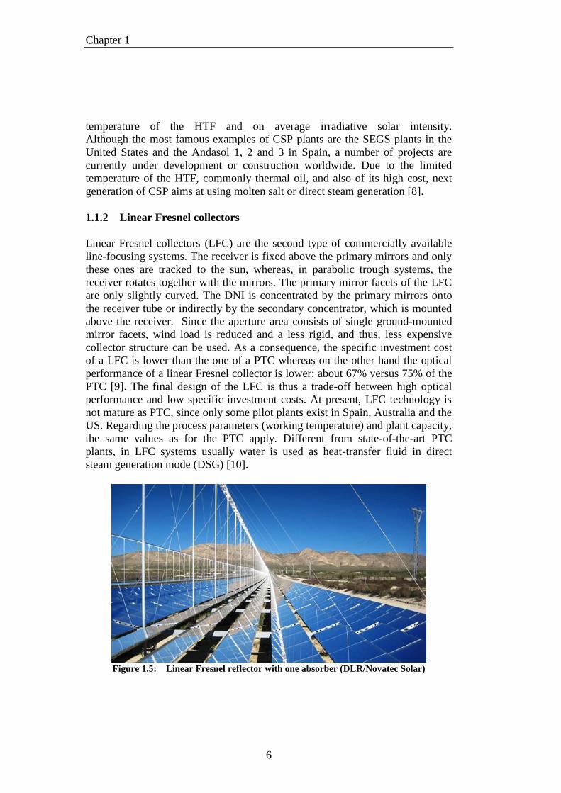
Linear Fresnel collectors (LFC) are the second type of commercially available
line-focusing systems. The receiver is fixed above the primary mirrors and only
these ones are tracked to the sun, whereas, in parabolic trough systems, the
receiver rotates together with the mirrors. The primary mirror facets of the LFC
are only slightly curved. The DNI is concentrated by the primary mirrors onto
the receiver tube or indirectly by the secondary concentrator, which is mounted
above the receiver. Since the aperture area consists of single ground-mounted
mirror facets, wind load is reduced and a less rigid, and thus, less expensive
collector structure can be used. As a consequence, the specific investment cost
of a LFC is lower than the one of a PTC whereas on the other hand the optical
performance of a linear Fresnel collector is lower: about 67% versus 75% of the
PTC [9]. The final design of the LFC is thus a trade-off between high optical
performance and low specific investment costs. At present, LFC technology is
not mature as PTC, since only some pilot plants exist in Spain, Australia and the
US. Regarding the process parameters (working temperature) and plant capacity,
the same values as for the PTC apply. Different from state-of-the-art PTC
plants, in LFC systems usually water is used as heat-transfer fluid in direct
steam generation mode (DSG) [10].
Figure 1.5: Linear Fresnel reflector with one absorber (DLR/Novatec Solar)
Concentrated solar power plants (CSP)
7
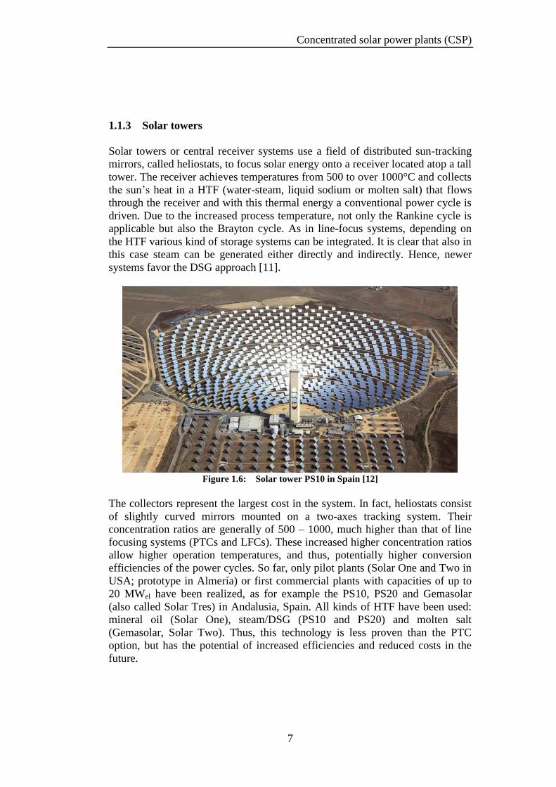
1.1.3 Solar towers
Solar towers or central receiver systems use a field of distributed sun-tracking
mirrors, called heliostats, to focus solar energy onto a receiver located atop a tall
tower. The receiver achieves temperatures from 500 to over 1000°C and collects
the sun’s heat in a HTF (water-steam, liquid sodium or molten salt) that flows
through the receiver and with this thermal energy a conventional power cycle is
driven. Due to the increased process temperature, not only the Rankine cycle is
applicable but also the Brayton cycle. As in line-focus systems, depending on
the HTF various kind of storage systems can be integrated. It is clear that also in
this case steam can be generated either directly and indirectly. Hence, newer
systems favor the DSG approach [11].
Figure 1.6: Solar tower PS10 in Spain [12]
The collectors represent the largest cost in the system. In fact, heliostats consist
of slightly curved mirrors mounted on a two-axes tracking system. Their
concentration ratios are generally of 500 – 1000, much higher than that of line
focusing systems (PTCs and LFCs). These increased higher concentration ratios
allow higher operation temperatures, and thus, potentially higher conversion
efficiencies of the power cycles. So far, only pilot plants (Solar One and Two in
USA; prototype in Almería) or first commercial plants with capacities of up to
20 MWel have been realized, as for example the PS10, PS20 and Gemasolar
(also called Solar Tres) in Andalusia, Spain. All kinds of HTF have been used:
mineral oil (Solar One), steam/DSG (PS10 and PS20) and molten salt
(Gemasolar, Solar Two). Thus, this technology is less proven than the PTC
option, but has the potential of increased efficiencies and reduced costs in the
future.

Chapter 1
8
1.1.4 Parabolic dish
Parabolic dish systems are point-focus collectors that track the sun on two axes
like solar towers. They use a large parabolic silvered mirror as reflector to
concentrate the sun’s radiation onto a receiver, which is mounted above the dish
at the focal point of the reflector. The receiver absorbs the reflected radiation
and converts it into thermal energy. This heat can either be used directly in order
to support chemical processes, but its most common application is power
generation. The thermal energy is converted directly to electricity with a Stirling
engine, connected to the receiver. In that manner, in contrast to parabolic trough
systems, dish systems can generate electricity independently without piping
losses or auxiliary consumption. Since parabolic dish collectors always point to
the sun, their optical losses are lower than these of parabolic trough, Fresnel or
tower systems. Dish units generally operate at concentration ratios of 600 up to
3000 which results in potentially highly efficient power conversion. In parabolic
dish collectors temperatures of more than 1500°C can be reached [13]. Their
principal advantages are a high solar-to-electricity conversion efficiency (over
30%) [14], modularity and flexibility. Due to wind loads, the size of the
parabolic mirror is limited and the typical capacity of a single system is
approximately 10 – 25 kWel. Therefore, dish systems are particularly well suited
for decentralized power supply and remote stand-alone power systems, such as
water pumping or village power applications [15].
Figure 1.7: Parabolic dish (DLR)

Concentrated solar power plants (CSP)
9
1.2 Overview of existing parabolic trough power plants
There are two ways to integrate a PTC solar field in a Rankine steam cycle
power plant:
1. indirectly, by heating a heat transfer fluid (HTF), typically a synthetic
oil, in the solar field and using it to produce steam through a heat
exchangers train;
2. directly, that is, generating steam in the solar field (DSG).
In both cases, with the thermal energy produced by the solar field a conventional
steam cycle can be driven, such as Rankine with Superheat (SH), Rankine with
Reheat (RH) and Rankine with Regeneration (RRg). Another option is an
Organic Rankine Cycle (ORC), where water is replaced by an organic fluid that
evaporates at a much lower temperature. If the radiation is sufficient, the system
can work at operating full capacity only with the solar field. In order to ensure
the production of electricity during periods of low radiation or during the night,
the plants usually are equipped with an additional back-up boiler and some of
them even with a TES.
Although the first PTC used DSG technology, and research in this area started in
the 80s, at the same time as the commercial use of the HTF technology, during
the last three decades commercial projects have not decided for it, due to the
potential problems and uncertainties associated with the two-phase water/steam
flow in the absorber tubes [8].
1.2.1 Parabolic trough plants with thermal oil
The SEGS plants were the first commercial power plants with thermal oil as
heat transfer fluid. Being built from 1985 to 1991 in the Mojave Desert in
California these plants are still in operation. The technology has proven to be
commercially ready and new power plants, like the Andasol 1, 2 and 3 in Spain,
are still based on the same system.
Figure 1.8 shows that the power plant can be subdivided into four locally
separated units: the collector field, the storage system, the back-up-system, and
the power block (PB). These systems consist fundamentally of two separate
fluid circuits: a HTF circuit and a water steam circuit. The HTF is heated up
from 290°C to 393°C inside the receiver tube of the solar field in order to return
to a series of heat exchangers in the PB, where it is used to generate high-
pressure superheated steam (100 bar, 371°C) for the power block. The PB is a
conventional thermal power station made up of several components like those

Chapter 1
10
used in fossil fuel power stations. The thermal energy of the steam is converted
into mechanical energy by a steam turbine and finally to electric energy by a
generator.
Figure 1.8: Schematic configuration of a parabolic trough power plant with oil as HTF
(Flabeg Solar International)
In state-of-the-art parabolic trough plants, synthetic oil is used as HTF. The
reason is that the vapor pressure of the thermal oil is much lower than that of
water. Therefore, even at temperatures that are above the critical point of water
(374°C), processes with thermal oil can remain in the liquid phase.
The thermal oil most widely used for temperatures up to 395°C is Therminol
VP-1, which is an eutectic mixture of 73.5% biphenyl oxide and 26.5%
diphenyl. Although it is flammable, safety and environmental protection
requirements can be satisfied. The main limitations are its chemical stability that
limits the maximum temperature of the steam Rankine cycle and the costs of the
oil-related equipment [16]
The selection of the HTF affects also the type of TES that can be used in the
power plant. Nowadays, the most commonly used storage concept in parabolic
trough systems with thermal oil is the indirect two-tank storage system with
molten salt (Andasol power plants, Spain). An indirect two-tank storage system,
as the name said, uses two reservoirs, a hot and a cold tank to store thermal
energy. In comparison with oil, molten salt presents some advantages as it is
non-flammable, non-toxic and has a lower cost.

Concentrated solar power plants (CSP)
11
1.2.2 Parabolic trough plants with molten salt
An innovative possibility is using molten salt as HTF in the solar field, instead
of thermal oil, in order to allow using the same fluid in both the SF and the TES
[17]. If molten salt is used in this way, the TES concept will become direct.
Figure 1.9 shows a schematic configuration of a solar power plant with PTCs
and molten salt as HTF.
Figure 1.9: Schematic configuration of a parabolic trough power plant with molten salt
as HTF (DLR)
If enough solar radiation is available, the molten salt from the cold tank is
pumped through the solar field, heated up to the design temperature and finally
stored in the hot tank. An auxiliary heater connected parallel to the collector
field, can also heat the molten salt to the design temperature. As long as there is
hot salt available in the hot tank, electricity can be produced on demand. As in
case of thermal oil, the molten salt circulates through a heat exchanger in order
to produce steam in the power block, and returns to the cold tank.
This technology offers a significant reduction in the cost of TES, eliminating the
need of heat exchangers, and allows reaching a higher maximum temperature in
the cycle compared to the one with synthetic oil. On the other side the
disadvantage is that molten salt freezes at relatively high temperatures (220°C in
the case of Solar Salt [18]) and much more care must be taken to make sure that
the salt HTF does not freeze in the solar field.

Chapter 1
12
A demonstration plant using this kind of technology was developed in Italy near
Syracuse in 2004 by a joint venture between ENEA and ENEL, along with other
smaller private companies, through a project called Archimede [19].
1.2.3 Parabolic trough plants with DSG
DSG refers to the direct generation of steam in the solar field, which makes the
steam generator unnecessary. The solar field is divided into different sections
performing the various stages of heat exchange: preheating, evaporation and
superheating. Figure 1.10 shows the overall scheme of a parabolic trough power
plant with DSG in the solar field.
Figure 1.10: Schematic configuration of a parabolic trough plant with DSG (DLR)
Only in the recent years parabolic trough systems with DSG have been
successfully tested under real solar conditions at the Plataforma Solar de
Almería for example during the DISS (Direct Solar Steam) [20, 21] and
INDITEP [22] projects. DSG has technical advantages over HTF technology
[23]. With this configuration the steam temperature is not limited by thermal oil,
but can reach values from 400°C to 550°C, increasing the thermal efficiency of
the Rankine cycle. Although DSG increases the cost of the solar field piping by
increasing the solar field fluid working pressure to above 100 bar, DSG leads to
a simplified plant configuration that reduces the investment and O&M costs.
Due to the constant temperature during phase transition, the thermal efficiency
Concentrated solar power plants (CSP)
13
of the collector is higher. Furthermore, compared to systems with thermal oil, in
DSG systems the overall plant efficiency increases while environmental and
operational risks, as fire hazard in case of leaks, are reduced.
The disadvantages of this technology concern the use of water/steam as a two-
phase flow. In fact, the required control systems are more complex and
expensive, due to the two-phase flow inside the absorber tubes and the different
thermodynamic properties of water and steam.
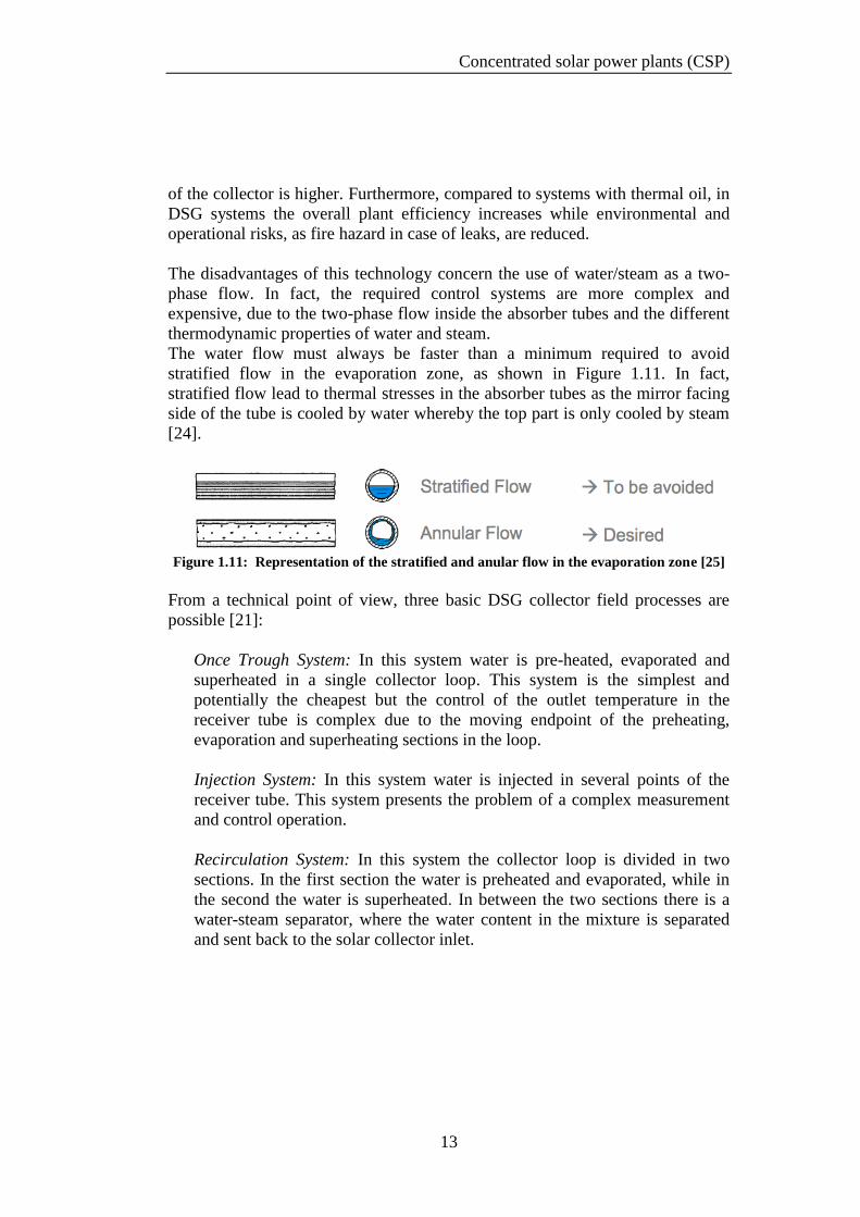
The water flow must always be faster than a minimum required to avoid
stratified flow in the evaporation zone, as shown in Figure 1.11. In fact,
stratified flow lead to thermal stresses in the absorber tubes as the mirror facing
side of the tube is cooled by water whereby the top part is only cooled by steam
[24].
Figure 1.11: Representation of the stratified and anular flow in the evaporation zone [25]
From a technical point of view, three basic DSG collector field processes are
possible [21]:
Once Trough System: In this system water is pre-heated, evaporated and
superheated in a single collector loop. This system is the simplest and
potentially the cheapest but the control of the outlet temperature in the
receiver tube is complex due to the moving endpoint of the preheating,
evaporation and superheating sections in the loop.
Injection System: In this system water is injected in several points of the
receiver tube. This system presents the problem of a complex measurement
and control operation.
Recirculation System: In this system the collector loop is divided in two
sections. In the first section the water is preheated and evaporated, while in
the second the water is superheated. In between the two sections there is a
water-steam separator, where the water content in the mixture is separated
and sent back to the solar collector inlet.

Chapter 1
14
Figure 1.12: Three basic DSG processes (DISS)
The projects DISS and INDITEP have shown that the recirculation concept is
the most feasible option for commercial application. Test results showed good
stability of the recirculation process even with a low recirculation ratio, thus,
making possible the use of small inexpensive water/steam separators in the solar
field [26]. In order to further bring down the costs of a DSG solar field, the
once-through concept is currently under development and demonstration
through the research project DUKE [27].
The two-phase fluid poses a major challenge and current state-of-the-art TES are
not suitable for DSG plants as they are not cost-competitive for large storage
capacities. Therefore, different projects and development activities were
performed in order to find innovative storage concepts. In the DISTOR project
performed by DLR, a storage system, subdivided in three parts, was proposed. A
phase change material (PCM) storage system was used to store latent heat of the
evaporation phase and a concrete storage system for the sensible heat during the
pre-heat and the super-heating phase [28, 29]. Another attractive option for
facilitating the operation of DSG plants in case of saturated cycles is represented
by short time direct storage systems called steam accumulators [30]. A system
analysis, including integrated TES, pointed out the large influence of TES on the
project investment cost of a DSG plant. A big effort in the development of a
commercial storage system for DSG is still needed to make this kind of plant
competitive in the market [31].

Concentrated solar power plants (CSP)
15
1.2.4 Parabolic trough plants with ORC
In the recent years several ORC companies investigated the integration of an
organic Rankine cycle, typically used in geothermal and biomass applications,
with parabolic trough solar systems (Figure 1.13). Systems under consideration
range in size from 100 kWel to 10 MWel.
Design studies indicate that optimized ORC systems, in those cases, could be
more efficient than more complex steam cycles operating at the same solar field
outlet temperature [7]. The general concept is to create a Micro CSP system that,
like a traditional trough plant, consists of a solar field circuit and an ORC power
block connected via a heat exchangers train. The main difference is that the
whole system with the ORC is smaller, modular and highly packaged. An ORC
optimized for a 300°C operating temperature should allow a significant increase
in the efficiency of small-size parabolic trough plants. In addition, at these
temperatures, thermal storage is economically feasible.
Figure 1.13: Schematic configuration of a parabolic trough power plant with ORC [5]
NREL analyzed a 1-MW ORC trough plant configuration in Saguaro, Arizona.
The Saguaro solar power plant, completed in 2006, is the first to combine solar
trough technology with an ORC power block provided by Ormat. N-pentane is
the selected working fluid, allowing for a cycle efficiency higher than 20%, with
an overall solar-to-electricity efficiency at the design point of 12.1% [32, 33]. The second micro-scaled CSP plant is the Holaniku at Keahole Point, developed
by Sopogy in the Kona desert, Hawaii. The plant produces 2 MW of thermal
energy that can be used to generate up to 500 kW of electricity through an ORC
power block. In addition, the site includes up to two hours of thermal energy
storage based on the indirect-two-tank storage system [34].

Chapter 1
16
.

17
2 Organic Rankine Cycle Background
During the last two decades a great interest has risen in Organic Rankine Cycles,
mainly because of the possibility to exploit heat sources at low and medium
temperature. Water is the working fluid of choice for the vast majority of large
scale fossil-fired Rankine cycle powerplants. Steam Rankine cycles are well-
suited for high-temperature applications, but generally at low temperatures the
efficiency decreases significantly. ORC is a promising technology for
decentralized power applications typically of the order of less than a few MW.
There is a variety of ORC fluids with different thermodynamic characteristics
available suited for different working temperature ranges. Therefore, one of the
advantages of ORC processes is that the working fluid can be selected according
to the temperature range of the heat source and heat sink. For example, ORC
systems can be used in biomass-fired combined heat and power systems, solar
thermal systems, geothermal systems and industrial waste heat recovery. The
modularity and versatility of this technology allows also for the integration of
ORC into small-scale combined cycle power plants as a bottoming cycle.
The chapter is organized as follows. In Section 2.1 a typical ORC configuration
is introduced and discussed. Section 2.2 presents the main characteristics of pure
organic fluids together with a briefly discussion regarding the possibility of
using mixtures. In Section 2.3 the main differences between steam Rankine
cycles and ORCs are highlighted, in particular focusing on thermodynamic
properties and turbine design considerations. Finally, Section 2.4 shortly
reviewed the state-of-the-art ORC applications and some of the most innovative
concepts being studied recently.

Chapter 2
18
2.1 Typical configuration
The basic principles of the Organic Rankine Cycle (ORC) are similar to those of
the steam Rankine cycle, but the main difference is that an organic working
fluid with a lower boiling point and a higher vapor pressure is used instead of
water. As shown in Figure 2.1, in the ideal cycle four processes can be
identified:
1. Isentropic pump (1 – 2) 2. Isobaric evaporation (2 – 5): The boiler can be divided into three
zones: preheating (2 – 3), evaporation (3 – 4) and superheating (4 – 5).
3. Isentropic expansion (5 – 6) 4. Isobaric condensation (6 – 1): The heat exchanger can be subdivided
into the desuperheating (6 – 7) and the condensation (7 – 1) zones.
In the real cycle, the presence of irreversibilities lowers the cycle efficiency.
These irreversibilities mainly occur during the expansion, in the heat exchangers
and in the pump [35].
Figure 2.1: T-s diagram for the ideal/real ORC cycle using isopentane as working fluid

Organic Rankine Cycle Background
19
ORC presents a layout simpler than that of the conventional steam Rankine
cycle: there is an evaporator or single heat exchanger to perform the three
evaporation phases (preheating, evaporation and superheating), an expansion
turbine, a condenser and a pump. In such systems, a regenerator is normally
installed between the pump outlet and the turbine outlet to improve the
performance of the system. The regenerator recovers the heat from the turbine
exhaust to preheat the liquid in order to reduce the amount of heat released and
the one needed to vaporize the fluid in the evaporator. Figure 2.2 shows a
typical configuration of an ORC with (right) and without (left) regenerator.
Figure 2.2: Component diagrams of a basic ORC (left) and a regenerative ORC (right)
[36]
Compared to conventional water steam cycles, ORC systems are less complex
and need less maintenance, which is partly explained by their modular feature: a
similar ORC system can be used, with little modifications, in conjunction with
various heat sources and applications, as presented further [36].

Chapter 2
20
2.2 Organic working fluids
The major difference between an ORC cycle and a conventional steam Rankine
cycle is the working fluid. An organic compound refers to all those chemical
compounds containing carbon with the exception of carbon oxides and derived
salts. Organic compounds consist of a structure of carbon and hydrogen atoms,
possibly combined with atoms of other chemical elements, such as nitrogen,
sulfur, phosphorus, silicon, fluorine and chlorine. Both pure fluids and fluid
mixtures proposed for ORC are classified as hydrocarbons and fluorocarbons,
refrigerants, aromatic compounds, paraffins, siloxanes, and inorganic fluids. The
thermodynamic performance of the cycle depends greatly on the type of fluid
chosen to take advantage of the available heat source. As we will see in Chapter
3, the selection of the organic fluid plays the real key role.
2.2.1 Characteristics of the organic working fluids
In order to be able to exploit heat sources at variable and medium-low
temperatures, it is necessary to make use of working fluids which certain
properties, such as the low boiling point and with curves that adapt well to
variations in the temperature of the sources themselves. In these cases, water
loses much of its utility and the fluids thermodynamically more interesting are
usually those organic compounds characterized by a high molecular mass, very
complex molecules and sufficient thermal stability. The organic substance
employed is usually characterized by a low boiling point, a low latent heat of
evaporation and high density; such properties are preferable to increase the input
flow to the turbine. Table 2.1 lists some organic fluids and their relevant
thermodynamic properties: water is included for comparison. Organic fluids
show a relatively lower heat of evaporation than that of water as a result of their
higher molecular mass. This is the main reason for which organic fluids are used
instead of water for heat recovery of low-medium temperature sources. In these
cases, ORCs allow to achieve better efficiencies and higher power compared to
conventional working fluids.
Table 2.1: Thermal properties of water and some organic working fluids
Working
fluid
Molecular
weight
(kg/kmol)
Boiling
Point (K)
Liquid
density
(kg/m3)
Latent heat
(kJ/kg)
Specific
heat ratio
water 18 373.15 958.35 2257.00 1.33
R-123 152.93 300.97 1456.7 170.19 1.10
isopentane 72.15 300.98 612.08 343.28 1.09
n-butane 58.12 272.66 601.26 385.71 1.12

Organic Rankine Cycle Background
21
Figure 2.3: T-s diagram of water and various ORC fluids [37]
2.2.2 Classification of fluids based on the T-s diagram
Organic fluids, depending on the slope of the saturation vapor curve on a
temperature-entropy diagram ( ), can be classified into three groups:
1. Dry fluids, characterized by a positive slope and a large molecular
weight; in this case the saturation curve in the T-s diagram is called
retrograde.
2. Wet fluids, characterized by a negative slope and a low molecular
weight.
3. Isentropic fluids, characterized by an infinite slope; in this case the
saturation curve is almost vertical.

Chapter 2
22
Figure 2.4: Saturation curves of a dry, wet and isentropic fluid [38]
Since the value of leads to infinity for isentropic fluids, the inverse of the
slope of the curve, defined as , is used as a parameter to express the
type of the fluid ( > 0: dry fluid, < 0: wet fluid, 0: isentropic fluid) [38].
The type of saturation curve is closely related to the number of atoms of the
molecule. The retrograde bells are typical for high molecular weight fluids, with
a high number of atoms greater than 12, while the classic bells similar to that of
water are typical of fluids with less than 8 atoms and smaller molecular weight
[39].
Figure 2.5: Effect of molecule size on the slope
Wet fluids are generally not suitable for ORC systems, because they require
large enthalpy to become saturated and need to be superheated in order to avoid
condensation during the expansion process and reduce the risk of blade erosion.
Dry and isentropic fluids have better thermodynamic efficiencies, because they

Organic Rankine Cycle Background
23
do not require superheating. If the slope of the saturation curve is too positive,
the fluid may exit the turbine at high temperatures; in this case, a regenerator is
introduced in order to take advantage of the thermal energy of the fluid.
A first selection of the fluid is carried out according to the slope of the saturation
curve and organic fluids considered are usually either dry or isentropic.
2.2.3 Mixtures
Most of ORC applications are focused on pure component working fluids.
However in some scientific work the utilization of organic fluid mixtures as
working media for Rankine power cycles [40, 41] are mentioned as interesting.
The main advantage in comparison to pure substances is represented by a non-
isothermal phase change that leads to a better matching of working fluid and
source/sink heat capacities. Figure 2.6 shows qualitatively the nature of the
phase change for a two-component mixture in the T-s and T-x diagrams.
Figure 2.6: Qualitative representation of an isobaric phase change for a two-components
mixture in the T-s and T-x (x = mole fraction) diagrams [40]
The compositions of liquid and vapour vary continuously along the isobar, and
the compositions in the two phases are not the same. Another difference
between mixtures and pure fluids occurs in the critical region. In this case, the
critical point is not anymore characterised by the maximum value of temperature
and pressure at which vapour and liquid coexists.

Chapter 2
24
2.3 Comparison with the steam Rankine cycle
2.3.1 Thermodynamic and physical differences
Water and organic fluids are characterized by different properties, as
summarized in Table 2.2. Water is inexpensive, non-toxic, non-flammable,
chemically stable, has low environmental impact and low viscosity (and thus,
lower friction losses and higher heat exchange coefficients). On the other hand,
organic fluids may be relatively toxic and more expensive than water. With its
low boiling point, a properly selected organic fluid can recover heat at much
lower temperatures when compared to steam Rankine cycles.
Table 2.2: Summary of fluids properties comparison in steam and organic Rankine
cycles
Steam Cycle Organic Rankine Cycle
Fluid Water Organic compound
Critical pressure High Low
Critical temperature High Low
Boiling point High Low
Condensing pressure Low Acceptable
Specific heat High Low
Viscosity Low Relatively high
Flammability No Yes, and depends on fluid
Toxicity No Yes, and depends on fluid
Environmental impact No High and depends on fluid
Availability Available Supply problem
Cost Cheap Expensive
As mentioned before, many of the thermodynamic characteristics and
technological properties of an ORC are closely related to the position and shape
of the saturation curve in the T-s diagram. Water is classified as a wet fluid,
while the ideal fluids for ORCs are generally either dry or isentropic.
The first main difference between organic fluids and water in a Rankine cycle is
their behavior when expanding from a saturated state through a turbine at low to
moderate temperatures (200 - 400°C), as shown qualitatively in Figure 2.7.
In conventional Rankine cycles the isentropic expansion phase of water in the
turbine occurs with a relatively low-quality two phase mixture (< 80%), while in
ORCs it can take place without condensation phenomena, giving a very high
performance and avoiding equipment damage. Hence, steam Rankine cycles
require higher turbine inlet temperatures than ORC, leading to a more complex
design characterized by superheating and reheating. This requires the use of

Organic Rankine Cycle Background
25
expensive high temperature materials for the turbine blades and the boiler.
In ORC systems, the turbine inlet temperatures are limited by the thermal
stability of the fluid. Dry and isentropic organic fluids exit the turbine at a
higher temperature than the condensing temperature. The available energy in
this superheated turbine exhaust also gives the opportunity for energy recovery
through a regenerator not present in a steam Rankine cycle, as discussed in
Section 2.1.
Figure 2.7: Rankine cycle for water (a) and for dry organic fluids (b)
In order to achieve high efficiencies, the condensing pressures of a steam
Rankine cycle are extremely low, typically between 0.05 and 0.1 bar. The
inevitable result of these sub-atmospheric condensing pressures is the infiltration
of air in the circuit, and hence the need of a deaeration equipment. In contrast to
that, the use of organic fluids allows operating at condensing pressures usually
higher than the atmospheric pressure, while the saturation pressures, with equal
levels of thermal source, are much higher. Super-atmospheric condensation
enables the design of low or no-maintenance power cycles. This attribute is
highly-desirable in remote and low-output applications where a full-time
licensed maintenance staff is not a reasonable expectation. In contrast, the main
disadvantage of ORC systems is the lower heat transfer coefficients of heat
exchangers compared to the ones of water. This involves a reduction of the
global coefficient of heat exchange surfaces and consequently more requests and
therefore higher costs at the same thermal load of the heat exchanger.
Finally, an advantage of ORCs has also to be underlined in regard of
thermodynamic cycle configurations. The limited critical pressure of organic
fluids in comparison of that of water, makes supercritical cycles at low
temperatures practically feasible [42].
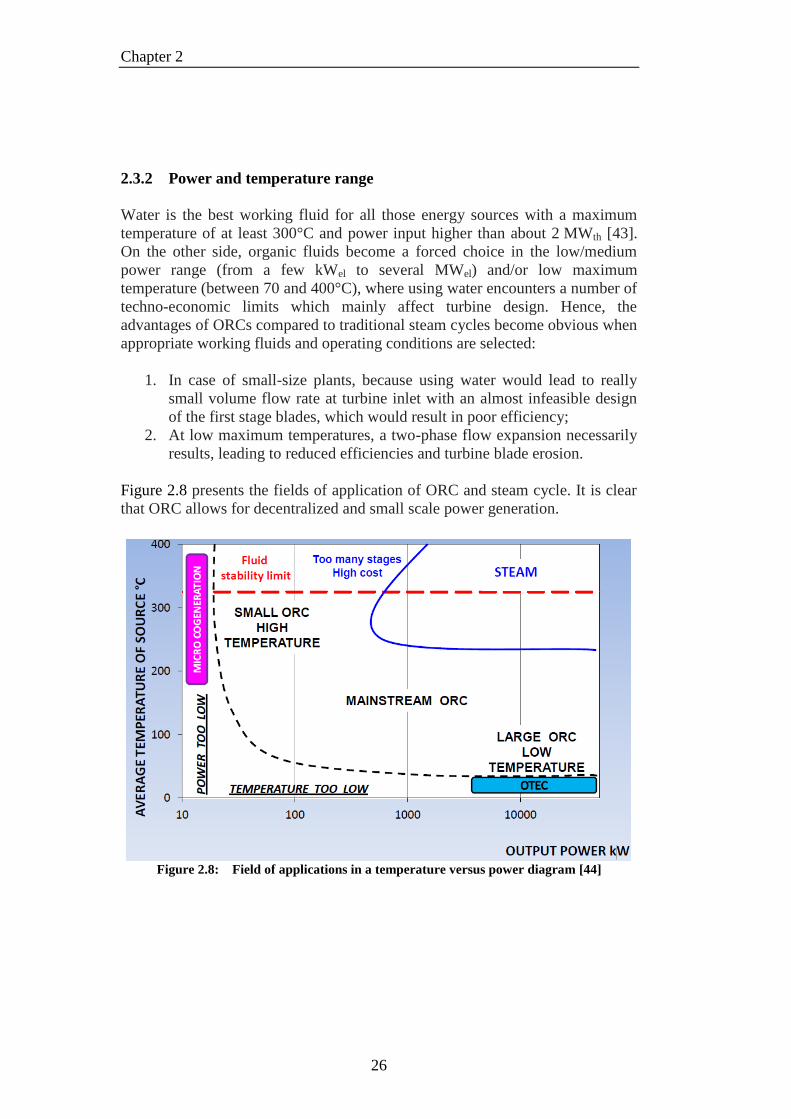
Chapter 2
26
2.3.2 Power and temperature range
Water is the best working fluid for all those energy sources with a maximum
temperature of at least 300°C and power input higher than about 2 MWth [43].
On the other side, organic fluids become a forced choice in the low/medium
power range (from a few kWel to several MWel) and/or low maximum
temperature (between 70 and 400°C), where using water encounters a number of
techno-economic limits which mainly affect turbine design. Hence, the
advantages of ORCs compared to traditional steam cycles become obvious when
appropriate working fluids and operating conditions are selected:
1. In case of small-size plants, because using water would lead to really
small volume flow rate at turbine inlet with an almost infeasible design
of the first stage blades, which would result in poor efficiency;
2. At low maximum temperatures, a two-phase flow expansion necessarily
results, leading to reduced efficiencies and turbine blade erosion.
Figure 2.8 presents the fields of application of ORC and steam cycle. It is clear
that ORC allows for decentralized and small scale power generation.
Figure 2.8: Field of applications in a temperature versus power diagram [44]
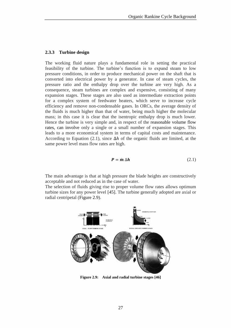
Organic Rankine Cycle Background
27
2.3.3 Turbine design
The working fluid nature plays a fundamental role in setting the practical
feasibility of the turbine. The turbine’s function is to expand steam to low
pressure conditions, in order to produce mechanical power on the shaft that is
converted into electrical power by a generator. In case of steam cycles, the
pressure ratio and the enthalpy drop over the turbine are very high. As a
consequence, steam turbines are complex and expensive, consisting of many
expansion stages. These stages are also used as intermediate extraction points
for a complex system of feedwater heaters, which serve to increase cycle
efficiency and remove non-condensable gases. In ORCs, the average density of
the fluids is much higher than that of water, being much higher the molecular
mass; in this case it is clear that the isentropic enthalpy drop is much lower.
Hence the turbine is very simple and, in respect of the reasonable volume flow
rates, can involve only a single or a small number of expansion stages. This
leads to a more economical system in terms of capital costs and maintenance.
According to Equation (2.1), since of the organic fluids are limited, at the
same power level mass flow rates are high.
(2.1)
The main advantage is that at high pressure the blade heights are constructively
acceptable and not reduced as in the case of water.
The selection of fluids giving rise to proper volume flow rates allows optimum
turbine sizes for any power level [45]. The turbine generally adopted are axial or
radial centripetal (Figure 2.9).
Figure 2.9: Axial and radial turbine stages [46]

Chapter 2
28
The first are the most commonly used and found major applications in processes
involving high volume flow rates and low enthalpy drops per stage, while for
the other is the opposite. Modern configurations tend to adopt a variable
geometry nozzle so as to optimize the efficiency of the expander in a wide range
of environmental conditions and to obtain high performance in off-design
conditions. The specific rotational speed of the turbine can be calculated with
Equation (2.2). From here, it can be inferred that a conventional steam turbine,
in which the outlet volumetric flow rates are reduced while the enthalpy drops
are high, requires a very high rotational speed. In this case the use of a gearbox
is indispensable. The use of organic fluids allows instead a direct coupling of the
turbine with the generator.
(√ )
( )
(2.2)
Therefore, another advantage resulting from the low rotational speed is a low
mechanical stress of the turbine.
2.4 ORC applications
Owing to its low operating temperature, an organic Rankine cycle can suitably
recover heat from various sources and this has already been demonstrated as the
number of ORC plants installed worldwide is steadily increasing (Figure 2.10)
[37].
Figure 2.10: ORC market evolution and share of each application in terms of number of
units adapted from [36]

Organic Rankine Cycle Background
29
The ORC technology is employed both in state-of-the-art and innovative
applications:
Biomass combined heat and power
Biomass is widely available in a number of agricultural or industrial processes
and can be used for the production of electricity in small to medium size scaled
power plants. The problem of high specific investment costs for classic
machinery such as steam boilers are overcome due to the low working pressures
in ORC power plants. For small decentralized units, combined heat and power
generation is required to ensure the profitability of the investment. Biomass
CHP plants are mostly limited to 6-10 MW thermal power, corresponding to 1-2
MW electrical power. Most of these installations are in Europe, such as the
plants built in Lienz Austria (1 MWel), Sauerlach Bavaria (700 kWel), Toblach
South Tyrol (1.1 MWel), and Fußach Austria (1.5 MWel) [47].
Geothermal Geothermal heat sources vary in temperature from a few tens of degrees up to
300°C. ORC is therefore perfectly adapted for this kind of application. These
types of power plants are binary cycle since two fluids are involved in the cycle:
liquid water/steam and the ORC cycle working fluid. However, it is important to
keep in mind that for low-temperature geothermal sources (typically less than
100°C), the conversion efficiency is very low and geothermal plants are not
economical. Higher temperature (> 150°C) geothermal heat sources enable
combined heat and power generation, allowing the cooling water to be used for
district heating. An example of a geothermal plant using the ORC process is the
plant Neustadt–Glewe in Germany, which was the first geothermal power plant
in Germany [48].
Waste heat recovery
Waste heat recovery is one of the most important development fields for ORC.
It can be applied to heat and power plants (e.g.: a small scale cogeneration plant
on a domestic water heater), or to industrial and farming processes such as
organic products fermentation, hot exhausts from ovens or furnaces, flue-gas
condensation or exhaust gases from vehicles. In such system, the waste heat is
generally recovered by an intermediate heat transfer loop and used to evaporate
the working fluid of the ORC.

Chapter 2
30
CSP solar power plant
ORC can be used in the solar parabolic trough technology in place of the usual
steam Rankine cycle in order to decrease investment costs at small scale. In fact,
ORC allows power generation at lower capacities and with a lower collector
temperature. Up to now, very few CSP plants using ORC are available on the
market [33, 49], as mentioned in Section 1.2.4. Some very small scale-systems
are being studied for remote off-grid applications, such as the proof-of-concept
3 kWel system developed for rural electrification of a clinic in Lesotho [50].
Solar pond power systems
In a solar pond power plant, a conventional ORC system takes advantage of
temperature gradients in salt-gradient solar pond systems. The maximum
temperature reached by the water stored in these ponds is about 90-100°C.
Solar ORC-RO desalination systems
A solar ORC-RO system couples a solar thermal engine and a reverse-osmosis
desalination plant. The solar thermal engine transforms the solar radiation into
mechanical power via an ORC. The useful shaft power by mechanical coupling
drives the high pressure pump of the RO desalination unit.
Ocean thermal energy conversion systems
This technology utilizes the temperature gradients (of at least 20°C) in oceans to
drive a binary cycle.
Cold production
The shaft power of the ORC system is used to drive the compressor of a
refrigeration system. This layout can be also used to produce heat if the ORC is
coupled to a heat pump.

31
3 The choice of the organic working fluid
Before we move on to study in detail the thermodynamic cycles, the important
matter of the choice of the organic working fluid has to be considered. In fact,
the working fluid plays a key role in the optimization of the cycle and its
selection has great implications for the design and performance of the whole
plant [45]. Several scientific studies on the selection of working fluids for
different types of heat sources and temperature ranges were carried out as for
example in [38, 51-53]. While there are many available choices for working
fluids, there are also many constraints on that selection that are related to the
thermodynamic properties of the fluids, as well as considerations of health,
safety and environmental impact. A set of possible working fluid candidates for
this work are identified using heuristic knowledge about the processes based on
similar systems. These candidates are then classified in respect of their operating
temperatures in low temperature (< 250°C) and high temperature (> 250°C)
fluids.
3.1 Selection criteria
In order to identify the most suitable organic working fluids the following
criteria are taken into account:
Thermodynamic properties
A good working fluid for the ORC applications should have the
following thermodynamic properties:
- an appropriate low critical temperature and pressure, in order to
allow performing supercritical cycles;
- high vapor density, in order to have an acceptable volume flow
rate;
- low viscosity in both the liquid and vapor phases, in order to
achieve high heat transfer coefficients and low friction losses in
the heat exchangers;
- high thermal conductivity, in order to achieve high heat transfer
coefficients in the heat exchangers.

Chapter 3
32
Thermal and chemical stability at operating temperatures
The maximum heat source temperature is limited by the chemical
stability of the working fluid in order to avoid deterioration and
decomposition at high temperatures.
Low or zero ODP (Ozone Depletion Potential)
ODP is a measure of the impact of a substance on the stratospheric ozone
layer measured relative to R11 (ODPR11 = 1) [54]. For currently used
fluids the ODP is less than 1, while it is always 0 for natural fluids.
Low or zero GWP (Global Warming Potential)
GWP is a measure of how much heat a substance traps in the atmosphere
and it is expressed as a factor of carbon dioxide, chosen at unity [55]. It
is calculated over a specific time interval, commonly 20, 100 or 500
years. The values have been defined for other fluids by the IPCC
(Intergovernmental Panel on Climate Change) [56] in 1994, but they are
constantly updated. For all synthetic fluids values are far greater than
one.
Low toxicity and flammability
The ANSI/ASHRAE Standard 34 [57] identifies two classes related to
toxicity and three groups related to flammability. For toxicity the TLV
(Threshold Limit Value) indicator is used. It is the level to which it is
believed an individual can be exposed day after day without adverse
health effects. The suffix TWA (Time Weighted Average) indicates the
average exposure to which an individual may be exposed during a usual
work week of eight hours a day for five days without suffering
consequences.
CLASS A: refrigerants with TLV-TWA > 400 ppm (lower toxicity)
CLASS B: refrigerants with TLV-TWA < 400 ppm (higher toxicity)
The three groups identified for flammability are the following:
GROUP 1: No flame propagation. Group consisting of all substances
that do not show flame propagation at a temperature of 21°C and at
atmospheric pressure.
GROUP 2: Lower flammability. Group consisting of all substances with
a lower flammability limit > 0.1 kg/m3 at a temperature of 21°C and at
atmospheric pressure and characterized by a heat of combustion
< 19 MJ/kg.
GROUP 3: Higher flammability. Group consisting of all substances with

The choice of the organic working fluid
33
a lower flammability limit ≤ 0.1 kg/m3 at a temperature of 21°C and at
atmospheric pressure and characterized by a heat of combustion
≥ 19 MJ/kg.
Table 3.1: Classification of Safety groups under the ANSI/ASHRAE Standard 34 [57]
Lower
Toxicity
Higher
Toxicity
Higher Flammability A3 B3
Lower Flammability A2 B2
No Flame Propagation A1 B1
According to Table 3.1, A1 fluids should be preferred.
Low costs and good availability
Fluids already used in commercial application are easier to obtain at a
reasonable cost.
In according to Drescher [58], the fluids might be chosen in the adequate
temperature range. The two main parameters are the maximum and minimum
process temperature. The upper limit of the maximum process temperature is the
fluid stability and material compatibility. The melting temperature should be
below the ambient temperature, otherwise the fluid may solidify during
shutdown time.
3.2 Screening of available fluids
Generally speaking, it is not easy to satisfy all the selection criteria mentioned
above, especially in case of high temperature applications, where the problem of
thermal stability became the important one. In order to identify the most suitable
fluids for a DSG application a pre-selection was made, taking into account fluids
that can be found in literature and state-of-the-art applications. Available fluids
were firstly compared on the basis of their chemical stability, flammability,
toxicity and potential to cause environmental harm. Cost was not considered as
an influential factor among fluids, since no accurate data were presented in order
to permit an appropriate evaluation.
The investigated organic fluids fall under five broad chemical groups:
1. Simple aliphatic hydrocarbons, such as butane, pentane, and hexane;
2. Fluorinated or halogenated hydrocarbons, including most refrigerants;

Chapter 3
34
3. Aldehydes and ketones – variations on simple hydrocarbons which can
be chosen so as to combine the benefits of hydrocarbons and
refrigerants;
4. Aromatic hydrocarbons, combining high stability with good expansion
properties and generally boiling well above ambient temperatures;
5. Siloxanes – a subgroup of silicones containing Si-O bonds with organic
radicals characterized by an extremely high chemical stability at high
temperatures.
Based on the critical temperature, which limits the evaporation temperature in
subcritical cycles, fluids can be grouped in three categories [37]:
1. High temperature fluids (Tcrit > 250°C)
2. Medium temperature fluids (150 < Tcrit < 250°C)
3. Low temperature fluids (Tcrit < 150°C)
Table 3.2: Classification of fluids based on their critical temperature
Low-temperature (LT)
(<150°C)
Medium-temperature (MT)
(150-250°C)
High-temperature (HT)
(>250°C)
Fluids Tcrit
(°C)
pcrit
(bar) Fluids
Tcrit
(°C)
pcrit
(bar) Fluids
Tcrit
(°C)
pcrit
(bar)
R32
Propane
R134a
R227ea
R152a
Ammonia
I-Butane
R236ea
78.1
96.7
101.1
101.8
113.3
132.3
134.8
139.3
57.82
42.51
40.59
29.25
45.17
113.3
36.29
35.02
N-Butane
R245fa
SES36
R123
R365mfc
N-pentane
Hexane
Methanol
Ethanol
MM
152.3
154.0
177.4
183.7
186.9
196.5
234.6
240.2
240.8
245.4
37.96
36.51
28.40
36.62
32.66
33.70
30.34
81.04
61.48
19.39
N-Heptane
Cyclohexane
Benzene
MDM
N-Octane
D4
Toluene
MD2M
D5
D6
N-Butylbenzene
Tribromomethane
267.0
280.5
288.9
291.1
296.2
313.3
318.6
325.8
346.1
372.7
388.0
422.9
27.36
40.75
49.06
14.15
24.97
13.32
41.26
12.27
11.60
9.61
n/a
n/a
As shown in Table 3.2, most of the typical working media adopted in low or
medium temperature applications are refrigerants. Figure 3.1 highlights the
relationship between the critical temperature and the critical pressure of the
screened working fluids. Fluids with high critical temperatures are characterised
by low critical pressures.

The choice of the organic working fluid
35
Figure 3.1: Critical temperature as function of the critical pressure of the screened
organic fluids
Chlorofluorocarbons (CFCs) and hydrochlorofluorocarbons (HCFCs) are not
considered in this screening, since some of them have already been phased out,
while some other will be phased out in 2020 or 2030 in accordance with the
Montreal Protocol established in 1987. For a long time this type of fluids have
been commercially available and rationally employed as working fluids for
ORC power generation from low-grade heat [45]. However, the inconvenience
is that their ozone-depleting potential is elevated. Hence, transitional
compounds, such as e.g. hydrofluorocarbons (HFCs) have been utilized to
replace them as refrigerants. Table 3.3 summarizes the most important
environmental characteristics of the working fluids, while Figure 3.2 gives a
graphical overview of the ODP and GWP, which are considered the most
important indexes.
Figure 3.2: Graphical overview of the ODP and GWP indexes of some organic fluids
0
50
100
150
200
250
300
350
400
450
0 50 100 150
T cr
it [
°C]
p crit [bar]
Ammonia
Siloxanes
Toluene
D6 D5
D4 MDM
MM
MD2M
SES36 R123 R245fa

Chapter 3
36
Table 3.3: Environmental characteristics of the investigated organic fluids
Fluids
TLV-
TWA
(ppm)
Autoignition
temperature
(°C)
Safety
group
Athmospheric
Lifetime
(yrs)
ODP
GWP
(100
yrs)
Water - - A1 n/a 0 <1
Methane 1000 580 A3 1
2 0 21
n-Butane 1000 405 A3 <1 0 ~0
i-Butane 1000 460 A3 <1 0 <10
Ammonia 25 651 B2 5-10 days 0 0
Propane 1000 450 A3 <1 0 ~0
Substances controlled and being phased out by the Montreal Protocol
CFC-11 1000 - A1 45 1 3800
CFC-12 1000 - A1 100 1 8100
CFC-13 1000 - A1 640 1
CFC-113 1000 - A1 85 1 4800
CFC-114 1000 - A1 300 1 8700
CFC-115 1000 - A1 1.7 0.44 8900
HCFC-22 1000 632 A1 12 .055 1500
HCFC-123 50 n/a B1 1.4 .02 90
Hydrofluorocarbons/Hydrocarbons
HFC-32 1000 648 A2 5.6 0 650
HFC-134a 1000 >743 A1 14.6 0 1300
HFC-152a 1000 455 A2 1.4 0 140
HFC-227ea 1000 n/a A1 34.2 0 2900
R236ea n/a n/a n/a 10.7 0 1200
HFC-245fa 400 412 B1 8.8 0 930
HFC-365mfc 1000 532 n/a 8.6 n/a 890
SES36 n/a 580 n/a n/a n/a n/a
n-pentane 600 309 A3 n/a 0 ~20
hexane n/a 234 n/a n/a n/a n/a
methanol n/a 385 n/a n/a n/a n/a
ethanol n/a 363 n/a n/a n/a n/a
n-heptane n/a 215 n/a n/a n/a n/a
cyclohexane n/a 245 A3 n/a n/a n/a
benzene n/a 555 n/a n/a n/a n/a
n-octane n/a 220 n/a n/a n/a n/a
toluene n/a 480 n/a 2-500 days n/a n/a
n-butylbenzene n/a 412 n/a n/a n/a n/a
tribromomethane n/a n/a n/a n/a n/a n/a
Siloxanes
MM n/a 340 n/a 10-30 days 0 n/a
MDM n/a 482 n/a 10-30 days 0 n/a
MD2M/MD3M/MD4M n/a n/a n/a 10-30 days 0 n/a
D4 n/a 384-387 n/a 10-30 days 0 n/a
D5 n/a 372 n/a 10-30 days 0 n/a
D6 n/a n/a n/a 10-30 days 0 n/a

The choice of the organic working fluid
37
3.2.1 ORC fluids classified by application
Currently, in mostly applications a limited number of fluids is used: refrigerants
and short chained alkanes are typically adopted for low temperature
applications, while siloxanes find their application in the higher temperature
range (300°C and above). For example, as shown in Table 3.4,
octamethyltrisiloxane (MDM) is already used in biomass cogeneration and heat
recovery applications (CHP) [5]. This fluid has advantages due to its favourable
thermodynamic properties (critical pressure and temperature), which leads to
high cycle efficiencies.
Table 3.4: Organic working fluid classified by application
Classification Application ORC working fluid
High Temperature
(> 250°C)
Biomass MDM
Waste heat recovery (WHR) Siloxanes
Low Temperature
(<250°C)
Waste heat recovery (WHR) R245fa
Solar thermal energy R245fa (HFC)
n-pentane
Geothermal n-perfluoropentane &
others
For each temperature there is a specific fluid and a specific cycle which allows
achieving the best efficiency. Some examples of studies on fluid and cycle
selection for different heat sources are presented in Table 3.5.
Table 3.5: List of studies on ORC fluids and cycle selection
Reference
Heat source
and temperature
range
Considered fluids Recommended
fluids and optimal
cycles
Drescher,
Brüggemann
(2006)
[58]
Biomass
@ 350°C
MDM, Toluene,
Ethylbenzene, Propylbenzene,
Butylbenzene
AlkylBenzenes:
TCond=90°C*
TEva=250-300°C
Borsukiewicz-
Gozdur, Novak
(2007)
[59]
Geothermal
@ 80-115°C
Propylene, R227ea, RC318,
R236fa, ibutane, R-245fa
Propylene,
R227ea, R-245fa:
TCond=25°C
TEva=80-115°C
Zhang, Jiang
(2012)
[60]
Geothermal
@ 100-200°C
R134a, R245fa, isobutene,
isopentane
Tbrine=100-150°C:
R134a
TCond=35°C
Tbrine=200°C:
R245fa
TCond=35°C

Chapter 3
38
Walraven et al.
(2012)
[61]
Geothermal
@ 100-150°C
R12, R22, R41, R32, R115,
R124, R125, R134a, R142b,
R152a, R218, R227ea,
R236ea, R236fa, R245fa,
R1234yf, R1234ze, RC318,
C4F10, C5F12, CF3I, SF6,
Ethane, Propane, iso-butane,
Propylene, DME, CO2, N2O,
others.
Tbrine=125°C,
no Tlimit,Geo:
R227ea
Tbrine=125°C,
Tlimit,Geo=75°C:
R1234yf
Badr, O’Callaghan
et al.
(1990)
[62]
WHR R11, R113, R114 R113:
TCond=30-50°C
TEva=120°C
Invernizzi et al.
(2007)
[63]
WHR:
MGT flue gas @
300°C
HFC-43-10mee, R123, n-
Pentane, R113, 2-2-
Dimethylbutane, 2-3-
Dimethylbutane, n-Hexane,
Hexafluorobenzene, MM,
Pentafluorobenzene, n-
Heptane, c-Hexane, MDM, n-
Octane, D4, MD2M
MM:
TCond=30°C
TEva=170°C
Lemort et al.
(2007)
[64]
WHR R245fa, R123, R134a, n-
pentane R123, n-pentane:
TCond=35°C
TEva=60-100°C
Liu, Chien et al.
(2004)
[65]
WHR R123, iso-pentane, HFE 7100,
Benzene, Toluene, p-xylene
Benzene, toluene,
R123:
TCond=30°C
TEva=150-200°C
Fahad A. Al-
Sulaiman
(2013)
[4]
WHR: steam
@ ~100°C
R600, R600a, R134a, R152a,
R290, R407c, and ammonia.
R134a:
TCond=35°C
TEva≈90°C
Dai, Wang et al.
(2009)
[66]
WHR: gas @
145°C
NH3, butane, isobutene, R11,
R123, R141B, R236ea,
R245ca, R113, water
R236ea:
TCond=25°C
TEva=87.7°C
iso-butane:
TEva=87.1°C
Lakew, Bolland
(2010)
[67]
WHR: air
@ 80-200°C
R134a, R123, R245fa,
R227ea, n-pentane, propane
Tha=80-160°C:
R227ea
TCond=20°C
Tha=200°C:
R245fa
TCond=20°C

The choice of the organic working fluid
39
Quoilin, Declaye et
al.
(2011)
[68]
WHR:
gas @ 180°C with
HTF.
R1234yf, R134a, R245fa,
HFE7000, SES36, R123, n-
butane, n-pentane
R245fa:
TEva=113.5°C
R123:
TEva=111.8°C
Schuster et al.
(2010)
[42]
Generic source
@ 210°C
Water, R134a, R227ea,
R152a, RC318, R236fa,
R245fa, isobutene, isopentane,
isohexane, cyclohexane,
R365mfc
Sup:
R365mfc & iso-
pentane:
TCond=20°C
Tmax≈180°C
Sub:
R245fa & iso-
butene:
TCond=20°C
TEva≈140°C
Tchanche,
Papadakis et al.
(2009)
[69]
Solar:
water
@ 90°C as HTF
Refrigerants R134a, R152a,
R600, R600a,
R290:
TCond=35°C
TEva≈75°C
Façao, Palmero-
Marrero et al.
(2008)
[70]
Solar
@ 80°C, 100-
150°C and 200-
250°C
Water, n-pentane, HFE7100,
cyclohexane, toluene, R245fa,
methanol, ammonia
Cyclohexane:
TCond=45°C
TEva=120-230°C
R245fa:
TCond=45°C
TEva=230-250°C
Quoilin,
Orosz et al.
(2011)
[50]
Solar:
with HTF
@ ~150°C
n-pentane, SES36, R245fa,
R134a
SES36:
TCond=30°C
TEva=169°C
n-pentane:
TCond=30°C
TEva=189°C * Min temperature of the heat sink instead of condensing temperature

Chapter 3
40
3.2.2 ORC fluids used by manufacturers
As mentioned in previous sections, fluid selection studies for different heat
sources and applications cover a broad range of working fluids. In fact, only a
few fluids are actually used by commercial ORC manufacturers.
ORC manufacturers constructed their first power plants in the beginning of the
80s [44]. The two main ORC manufacturers are Turboden and Ormat, the first
one mainly focused on biomass boilers and other high temperature applications,
the second one mainly interested on the geothermal market and on machines for
remote installations.
It is generally difficult to find out details on the working fluids the ORC
manufacturers use in their applications. However, Table 3.6 represents a list of
the most famous ORC manufacturers and the related available informations. The
fact that the fluids listed are already used in commercial applications, makes
them promising candidates for this master thesis, because they are supposed to
be available on the market.
Table 3.6: List of the main ORC manufacturers and used working fluids
Manufacturer Applications
Power
range
(kWe)
Heat source
temperature
(°C)
ORC working
fluid
Turboden
Biomass-
CHP, WHR,
Geo.
200-2.000 100-300 Solkatherm
(SES36), MDM
Ormat Geo., WHR,
Solar 200-70.000 150-300
Isopentane, n-
pentane & co.
Ingeco
STG International
Electratherm Green
machine
Verdicorp
Bosch KWK
WHR, Solar
WHR
50
30-75
65-325
>93
n/a
120-150
R245fa (HFC)
Exergy WHR, Geo.,
Biomass n/a n/a
PP1, isobutene,
R245fa
Infinity Turbine
Cryostar WHR, Geo. n/a 100-400 R134a, R245fa
TriOGen WHR 160 >350 Toluene

The choice of the organic working fluid
41
3.3 Suitable organic fluids for DSG
A relatively large group of substances has been considered in this study,
comprising fluids both for low and high temperature applications, belonging to
families such as linear and aromatic hydrocarbons, refrigerants (HFC) and
siloxanes. In particular, the organic fluid that circulates through the solar field
must meet basic requirements as safety and technical suitability. In this sense
toxic fluids or substances harmful to the ambient should not be taken into
consideration. Flammable compounds should also be avoided, even if
appropriate safety measures could be provided.
The investigated fluids have been selected in order to deal with different
maximum temperature values between 200°C and 400°C, typical values reached
from existing CSP systems. There is no optimal fluid that meets all the selection
criteria discussed in Section 3.1. Therefore, a trade-off must be made.
When the maximum temperature is low, a refrigerant fluid (like R245fa) with a
low critical temperature can be used; as the maximum temperature increases,
fluids with a higher critical temperature must be used. Among the fluids with an
elevated critical temperature found in literature, siloxanes are mentioned as the
most promising also due to their environmental friendly characteristics. They
allow operating a subcritical ORC with limited pressure. Figure 3.3 reports some
thermodynamic data of the selected fluids, showing the different critical
temperature and critical pressure and the limited temperature in accordance with
the thermal stability.
Figure 3.3: Critical temperature and pressure of the selected ORC fluid families

Chapter 3
42
3.3.1 LT fluids: R245fa, SES36
According to the selection criteria mentioned in Section 3.1, two fluids have
been selected among the original list of Table 3.2 for a DSG in case of low
temperature (< 250°C) applications: R245fa and SES36.
R245fa
R245fa is a HFC also known as pentafluoropropane and by its chemical name
1,1,1,3,3,-pentafluoropropane. From the corresponding T-s diagram, shown in
Figure 3.4, it could be considered as an isentropic fluid. Unlike CFC and HCFC,
it has no ODP and is nearly non-toxic. Its thermophysical properties and
environmental characteristics make it suitable for different applications, such as
centrifugal chillers, ORC for energy recovery and power generation, sensible
heat transfer in low-temperature refrigeration, heat pumps and passive cooling
devices. As well, it has a broad range of applications like foam blowing agent,
solvent and aerosol. Although it is intended to remain trapped within the foam
insulation, it is practically non bio-degradable with a lifetime of 8.8 years when
it eventually does escape into the atmosphere. It has a high GWP of 930, but
Honeywell refers to this as acceptable in their literature. Chemical analysis
confirmed that the fluid can be considered stable at 300°C [71]. One of the main
disadvantages of R245fa is instead the cost. Its actual price is continuously
rising, since the fluid is subjected to GWP taxes depending on the country
regulations [72].
Figure 3.4: T-s diagram of R245fa
Table 3.7: Thermodynamic properties of R245fa
Compound Molecular Mass,
(kg/kmol)
Critical Temp.,
(°C)
Critical pressure,
(bar)
Boiling Temp.,
(°C)
R245fa 134.05 154.01 36.51 15.3

The choice of the organic working fluid
43
Solkatherm® SES36
Solkatherm® SES36 is the brand name of an azeotropic binary mixture of 65%
of a hydrofluorocarbon, R365mfc and of 35% of a perfluoropoly-ether (PFPE)
manufactured by Solvay. A more comprehensive series of thermophysical
properties of Solkatherm can be found in [73].
Solkatherm could be a very interesting alternative to the hydrocarbons due to its
particular characteristics [74]: high molecular mass combined with favourable
transport properties, non-flammable, chemically stable, compatible with the
most construction materials and environmentally benign fluid. It is thermally
stable and it has been proved in continuous operation conditions up to 190°C (its
first decomposition reactions occur in laboratory at 220°C). It boils at a
relatively low temperature (36.7°C) and has been successfully adopted for the
first time as a working fluid by Turboden, Italy [5] in the case of the low
temperature geothermal binary plant of Altheim, Austria. Besides geothermal
power plants, other areas where Solkatherm could be used, are local combined
heat and power plants, solar-thermal systems, and high temperature heat pumps.
Figure 3.5: T-s diagram of Solkatherm® SES 36
Table 3.8: Thermodynamic properties of Solkatherm® SES36
Compound Molecular Mass,
(kg/kmol)
Critical Temp.,
(°C)
Critical pressure,
(bar)
Boiling Temp.,
(°C)
SES36 184.45 177.4 28.4 36.7

Chapter 3
44
3.3.2 HT fluids: Siloxanes
For high-temperatures applications, fluids with the highest possible critical
temperature should be selected. Among the investigated fluids with a higher
critical temperature, siloxanes allow operating a subcritical ORC with limited
pressure at high and medium temperatures. Siloxanes are a family of organic
compounds that contain silicon, oxygen and hydrocarbon groups. The main
advantages of this family of compounds are: low/non-toxicity, limited
flammability, good material compatibility, low foul formation over heat transfer
surfaces and a good thermal stability. Due to the high molecular complexity,
siloxanes are named by their compact units (M unit and D unit) and can be
divided in two main groups:
Linear siloxanes
1. MM (hexamethyldisiloxane, C6H18OSi2)
2. MDM (octamethyltrisiloxane, C8H24Si3O2)
3. MD2M (decamethyltetrasiloxane, C10H30Si4O3)
4. MD3M (dodecamethylpentasiloxane, C12H36Si5O4)
5. MD4M (tetradecamethylhexasiloxane, C14H42O5Si6)
Figure 3.6: T-s diagram and proven thermal stability limit of linear siloxanes [75]

The choice of the organic working fluid
45
Cyclic siloxanes:
1. D4 (octamethylcyclotetrasiloxane, C8H24O4Si4)
2. D5 (decamethylcyclopentasiloxane, C10H30O5Si5)
3. D6 (dodecamethylcyclohexasiloxane, C12H36Si6O6)
Figure 3.7: T-s diagram and proven thermal stability limit of cyclic siloxanes [75]
At ambient conditions, siloxanes are liquid and appear slightly viscous, odorless,
and transparent. Some of their thermodynamic characteristics are summarized in
Table 3.9. In principle, siloxanes can all be used as working fluids in ORC
turbines depending on the electrical power range [76]. They are already
employed as working media in high-temperature ORC applications (turbine inlet
temperature = 300°C) for larger power capacities (400 kWel – 2 MWel) and
mixture have been successfully adopted as HTF, comprising the CSP industry
(Syltherm 800 [77]).
Table 3.9: Thermodynamic properties of siloxanes
Compound Molecular Mass,
(kg/kmol)
Critical Temp.,
(°C)
Critical pressure,
(bar)
Boiling Temp.,
(°C)
MM 162.38 245.60 19.39 100.25
MDM 236.53 290.94 14.15 152.51
MD2M 310.69 326.25 12.27 194.36
MD3M 384.84 355.21 9.45 229.87
MD4M 458.99 380.05 8.77 260.75
D4 296.62 313.35 13.32 175.35
D5 370.77 346.00 11.60 210.9
D6 444.92 372.63 9.61 244.96

Chapter 3
46
Cyclic siloxanes are more stable than linear siloxanes. In a study of Angelino
and Invernizzi [78], it was suggested a thermal limit of cyclic siloxanes near to
400°C, ensuring 340°C by means of an experimental test in the presence of
oxygen and humidity. Cyclic stress can accelerate the thermal degradation of
siloxanes, although the addition of stabilizing agents may also be considered. In
present studies, the maximum temperature of the working fluid in the cycle is
usually fixed at 300°C for linear siloxanes and at 340°C for cyclic siloxanes
[75].

47
4 ORC processes analysis
The main objective of this chapter is to evaluate different cycle configurations in
order to choose the potential one that could be implemented in a solar field with
a feasible TES system. In order to take advantage of the achievable temperatures
of the PTCs and in accordance with the research fields of the Line Focus
Systems division of DLR, the main interest is set on high temperature processes.
Therefore, siloxanes are chosen as working fluids and the following single-
pressure level cycles are considered:
Subcritical saturated regenerative cycle
Superheated regenerative cycle
Supercritical regenerative cycle
Useful guidelines to select the most appropriate fluid among the siloxanes and to
define the operating parameters have been provided. In accordance with the
properties of linear and cyclic siloxanes, the minimum temperatures of the
analysed cycles are chosen to ensure a condensing pressure of at least 0.05 bar.
This pressure represents a technical limit as explained in Section 4.3. The
maximum obtainable temperatures are set well below the stability limit of the
selected fluids. After a first thermodynamic optimization of the fluids, the
analysis is focused on two particular siloxanes (MM and D4).
The thermodynamic analysis is made using Excel integrated with the CoolProp
add-in [79], an open-source library that uses accurate equations of state to
provide the thermodynamic and transport properties of 86 pure and pseudo-pure
fluids. It includes all significant ORC working fluids, as R245fa and siloxanes
(MM, MDM, MD2M, MD3M, MD4M, D4, D5, D6).
Once the cycles with the best performances are selected, a thermodynamic
assessment of different storage system integrations is perfomed with the aim of
finding the optimum configuration.
Figure 4.1: Flow chart of the performed analysis

Chapter 4
48
4.1 Regenerative cycles
Three basic configurations are considered: saturated, superheated and
supercritical cycles. The non-regenerative cycle configurations are not analysed,
because, as mentioned in Chapter 2, regeneration is always convenient in case of
organic dry fluids. It was shown that regenerative ORC has higher first and
second law efficiencies than basic ORC [80]. Due to the better efficiency, the
cycle needs less thermal energy for the same electricity yield. Regarding a solar
thermal ORC power plant, the size of the solar field and the overall cost of the
plant decrease.
Saturated cycle
In a saturated cycle the working fluid enters the turbine as saturated steam. A
representative cycle is shown in the T-s diagram in Figure 4.2. As a general rule,
owing to the high molecular complexity of the considered organic fluids,
saturated cycles are preferable. In contrast to traditional water steam cycles,
superheating is not strictly requested in terms of preventing moisture formation
during the expansion in the turbine, as already explained in Chapter 2.
Figure 4.2: Representative T-s diagram of a subcritical saturated cycle

ORC processes analysis
49
Superheated cycle
In a superheated cycle, after being evaporated the temperature of organic fluid
vapour is increased again in order to produce superheated steam before entering
the turbine. A simplified representation of the cycle is shown in Figure 4.3. As
said before, dry fluids do not need to be superheated in order to avoid the liquid
phase at the end of the expansion, but they were also presented in this
configuration cycle to obtain more knowledge of their behaviour. The impact of
superheating is determined by the rate at which the constant pressure lines
diverge [38]. For dry fluids the thermal efficiency of the cycle remains
approximately constant when the inlet temperature of the turbine is increased.
Moreover, in [80] it is shown that superheating in organic Rankine cycles
increases the irreversibility and decreases the second law efficiency. Therefore,
organic fluids should be operated at saturated conditions to reduce the total
irreversibility of the system.
Figure 4.3: Representative T-s diagram of a subcritical superheated cycle
Supercritical cycle
If thermal stability of the fluid allows operation at supercritical temperatures, the
working fluid can be compressed directly to a pressure higher than its critical

Chapter 4
50
one (Figure 4.4). Hence, the heating process does not pass through a distinct
two-phase region before expansion. Due to their low critical pressures, siloxanes
can also be used in supercritical cycles. In order to find the optimum pressure an
optimization study should be performed.
Figure 4.4: Representative T-s diagram of a supercritical cycle
4.2 Basic cycle analysis model
A first model is designed for a rapid screening of potential power cycle
configurations. Figure 4.5 shows a schematic representation of the ORC
components and the corresponding working fluid state points. Once fixed
variables are assigned, all the other thermodynamic points of the cycle can be
sequentially calculated. Working fluid enthalpy, temperature, pressure, entropy,
and specific volume are calculated for each inlet and outlet of every component
by solving mass and energy balances complemented by performance equations.
For simplicity, the internal irreversibility and the pressure drops in steam
generator, regenerator, condenser and pipes are ignored when the
thermodynamic properties are estimated. Each component is considered as a
steady-state steady-flow system and is described further.

ORC processes analysis
51
Figure 4.5: Schematic representation of ORC components and working fluid state points
Pump
The pump power can be expressed as
( )
(4.1)
where is the ideal power of the pump, is the working fluid mass flow
rate, is the isentropic efficiency of the pump, and and are the
enthalpies of the working fluid at the inlet and outlet of the pump for the ideal
case.
Heat input source
The heat source is equals to the solar thermal energy collected by the solar field.
The heat input rate is defined as
( ) (4.2)
where and are the enthalpies of the working fluid at the exit and inlet of
the solar field, respectively.
Simplified schematic ORC configuration
G
122*
3
5
4
Turbine
Pump
Condenser or CHP
Regenerator
GeneratorHeat
source

Chapter 4
52
Turbine
The turbine power is given by
( ) (4.3)
where is the ideal power of the turbine, is the turbine isentropic
efficiency, and and are the enthalpies of the working fluid at the inlet and
outlet of the turbine for the ideal case.
Regenerator
The heat rate recovered by the regenerator is
( ) ( ) (4.4)
The working fluid temperature at the regenerator outlet is calculated based on
the turbine outlet temperature, the pump outlet temperature, and the regenerator
effectiveness. Regenerator effectiveness is defined as
(4.5)
In accordance with the working fluid state points
(4.6)
Condenser
The condenser heat rate can be expressed as
( ) (4.7)
where and are the enthalpies of the working fluid at the inlet and outlet of
the condenser, respectively.

ORC processes analysis
53
Net power and performance indexes
Once all components are defined, the net power of the cycle is calculated by
(4.8)
Two Performance Indexes are normally introduced as key indicators of the ORC
potential. Equation (4.9) defines the thermal (first-law) efficiency as the ratio
between the net power of the cycle and the input heat rate.
(4.9)
Substituting Equation (4.1), (4.2) and (4.3) the cycle thermal efficiency for a
regenerative ORC can be written as
( ) ( )
(4.10)
The second performance index is the ORC net specific work (kJ/kg), defined as
(4.11)
4.3 Thermodynamic optimization of siloxanes
The choice of the optimal cycle configuration is strictly related to the considered
working fluid, since only a correct selection of both fluid and cycle
configuration allows achieving the best system performance [81].
Most of the works published in the literature deal with thermodynamic
assessments, i.e. they aim at maximizing the plant efficiency or its power output.
However, thermodynamic assessment alone cannot provide exhaustive
indications on the optimal working fluid, mainly because of the different
thermal and volumetric behaviour of the fluids, which affect the performance,
the size and the cost of the plant components [82]. The most important
parameters in evaluating the most suitable fluids are the power output of the

Chapter 4
54
system, the condensing pressure and the volume flow ratio in the turbine [83].
First of all, the working fluid selection must account for its consequences on the
turbine design. There is a strong relationship between the working fluid
properties and the turbine architecture (speed of revolution, number of stages,
dimensions) and performance (isentropic efficiency).
In order to select the proper fluid and its related cycle, all eight siloxanes, listed
in Table 4.1, are evaluated in according to the following criteria:
Condensing pressure;
Maximum temperature;
Volume flow ratio (Vr).
Table 4.1: Siloxanes data
Linear siloxanes Cyclic siloxanes
Fluids MM MDM MD2M MD3M MD4M D4 D5 D6
Tcrit (°C) 245.6 290.94 326.25 355.21 380.05 313.35 346 372.63
pcrit (bar) 19.39 14.15 12.27 9.45 8.77 13.32 11.6 9.61
Tmax (°C) 300 300 300 300 300 340 340 340
4.3.1 Condensing pressure
An ORC should operate at the minimum admissible condensing temperature,
assuring that the corresponding pressure is not too low. In accordance with
previous researches on ORC systems, the lowest technical limit for the
condensing pressure is considered to be 0.05 bar [83]. As can be seen in Figure
4.6, MM can be considered as the most suitable candidate in case of electricity
production, due to its high condensing pressures for the related low condensing
temperatures.
Due to the pressure limit the application of MDM and D4 in power cycles
entails relatively high condensing temperatures (66.5°C for MDM and 87.3°C
for D4). For that reason both fluids are typically used for combined heat and
power systems. With D5 and D6 the condensing temperature would be even
higher (> 100°C). For instance, Figure 4.6 shows that the use of D5 and D6, in
the considered temperature range leads to very low pressures not feasible for
actual condensers. MD2M, MD3M and MD4M are not represented in the figure,
but have similar characteristics. While in such cycles the electrical efficiency
decreases, rejected heat can be used for applications like CHP, absorption cycles
or district heating.

ORC processes analysis
55
Figure 4.6: Evaluation of condensing pressure and corresponding temperature for
siloxanes
4.3.2 Maximum temperature
The maximum temperature is assessed to ensure the thermal stability of
siloxanes. In case of saturated cycles a Tmax/Tcrit ratio lower than 0.95 is ensured.
If the fluid allows a maximum temperature higher than the critical one,
supercritical cycles can be realized. According to that, a value of 280°C was
chosen as Tmax in order to perform a saturated process analysis with the fluid D4
and a supercritical process analysis with the fluid MM at the same maximum
temperature. The analysis of the following sections refers to these two cycles. A
process with fluid MDM is not considered, since at 280°C the ratio Tmax/Tcrit is
too high, as shown in Table 4.2.
Table 4.2: Reducted temperature for siloxanes MM, MDM and D4 at a maximum
temperature of 280°C Fluids MM MDM D4
Tmax/Tcrit - 0.98 0.94

Chapter 4
56
4.3.3 Volume flow ratio
The use of different fluids implies a wide variation of turbine operating
parameters. In order to choose the appropriate working fluid it is necessary to
predict the turbine performance and optimize the turbine design variables as e.g.
number of stages, speed of revolution and relevant blade geometric parameters.
According to similarity rules, the efficiency of a turbine stage is primarily set by
its specific speed and specific diameter.
The most important parameters affecting the isentropic turbine efficiency are
defined as follows:
• Volume flow ratio (Vr)
(4.12)
• Size parameter (SP)
√
(4.13)
• Specific speed ( )
(√ )
( )
(4.14)
The isentropic Vr accounts for the effect of the compressibility through the
expansion, where and are respectively the outlet and inlet volume
flow rates, evaluated for a multistage machines at the exit of the last stage and at
the inlet of the first stage. Vr is variable and strictly dependent on the working
fluid considered [63]. Generally speaking, the turbine efficiency decreases by
increasing Vr because of the losses related to the occurrence of high Mach
numbers and, for reaction turbines, to the negative influence of wide flow area
variations across the rotor blades. Moreover, for multistage single-shaft turbines,
large Vr prevents operating the various stages at optimum specific speed. In the
analyzed case the value of Vr should be below 500 in accordance with the
considerations reported in [82].

ORC processes analysis
57
The SP is function solely of the thermodynamic cycle and power output, where
is the isentropic enthalpy drop in the turbine. Furthermore, SP is
proportional, for a given value of specific diameter to actual turbine
dimensions. Low SP values penalize turbine efficiency because of large losses
caused by the increase of relative blade thickness, clearances and roughness.
Since SP is defined with reference to the outlet volume flow rate, the
contemporary occurrence of high Vr and low SP yields leads to very small flow
areas in the first portion of the machine with further efficiency penalties [84].
Vr, SP and values are calculated for both chosen cycle configurations, under
different working conditions. Table 4.3 summarizes the assumed operating
parameters. For both configurations, the working fluid, turbine inlet pressure
and temperature, condensing temperature and components efficiencies are given
as inputs. The maximum temperature of the working fluid at the turbine inlet
Tmax is fixed at 280°C. In case of the subcritical saturated cycle, the turbine inlet
pressure pin,t directly depends on this parameter. In case of the supercritical
cycle, its critical pressure value is used as pin,t. The mass flow rate is equal in
both cases to 1 kg/s, in order to systematically compare the different cycles, with
fixed normalized mass flow conditions.
Table 4.3: Summary of fixed and parametric conditions used to define the studied cases
Cycle conditions Saturated cycle with
D4
Supercritical cycle
with MM
1 kg/s
Tmax 280°C
pin,t 8.076 bar 19.394 bar
Tc Parametric study
(25°C - 90°C)
83%
70%
90%
Figure 4.7 shows the values of Vr for different values of condensing temperature
at fixed Tmax for both analyzed cycles. The value for Vr of the supercritical cycle
is far below the allowed maximum of 500. Applying this limit to the saturated
cycle with D4, the condensing temperature must be above 70°C. Figure 4.8 and
Figure 4.9 shows the values of SP and Ns respectively. In order to allow the
direct drive of the electric generator without reduction gear, a low speed of
rotation N of 3000 rpm is assumed.

Chapter 4
58
Figure 4.7: Turbine isentropic volume flow ratio for an isentropic expansion as a
function of condensing temperature for a maximum cycle temperature of 280°C
Figure 4.8: Turbine size parameter as a function of condesing temperature for a
maximum cycle temperature of 280°C
Figure 4.9: Specific speed as a function of the condensing temperature for a maximum
cycle temperature of 280°C

ORC processes analysis
59
4.4 Thermodynamic analysis
The energy analysis based on the first law of thermodynamics is performed and
the two performance indexes and are carried out for both chosen cycle
configurations.
According to Figure 4.10 and Figure 4.11, adopting a supercritical cycle, in
comparison to a saturated one with the same condensing temperature, allows
achieving high performances in terms of specific net work, but decreases the
cycle efficiency.
Figure 4.10: Specific net work as a function of condensing temperature in both
configurations for a maximum cycle temperature of 280°C
Figure 4.11: Cycle efficiency as a function of condensing temperature in both
configurations for a maximum cycle temperature of 280°C

Chapter 4
60
In respect of the previous analysis, a value of condensing pressure pcond of
0.05 bar has to be ensured. Due to the different condensing conditions, the
supercritical cycle configuration is considered as a power-only application,
while the saturated one as a CHP application. The condensing pressure value
pcond is then increased in case of the supercritical cycle configuration with MM
to ensure a minimum condensing temperature Tcond of 45°C. This value allows
operating with air coolers. Table 4.4 reports the performance indexes and the Vr
values obtained in both configurations for the two different condensing
conditions.
Table 4.4: Different condensing conditions and perfomance indexes for both analyzed
configurations
Cycle conditions Saturated cycle
with D4
Supercritical cycle
with MM
Tcond 87°C 45°C
pcond 0.05 bar 0.141 bar
Performance
Index
23.413 % 27.786 %
56.126 kJ/kg 95.583 kJ/kg
Vr 231.836 171.123
It is important to highlight that the obtained cycle efficiency and specific net
work are just two parameters useful for the interpretation of the ORC itself, but
cannot be used as optimization parameters. A correct evaluation among the
different configurations should always refer to the whole net plant power output,
system efficiency or second law efficiency.
In order to evaluate the influence of the turbine inlet pressure on the cycle
efficiency for a supercritical cycle with fixed Tmax, a parametric study of pin,t
between 20-35 bar is performed. Figure 4.12 shows the study perfomed on the
supercritical cycle at different condensing temperatures. It came out that thermal
efficiency reaches its maximum value with a turbine inlet pressure close to the
critical pressure value and subsequently decreases slightly for pressures higher
than the critical one.

ORC processes analysis
61
Figure 4.12: Cycle efficiency as a function of turbine inlet pressure for a maximum cycle
temperature of 280°C in a supercritical cycle configuration with MM
Figure 4.13 shows in detail the changes of the enthalpy drops of the main
components for a condensing temperature of 45°C. Frome here, the following
conclusions can be drawn. As the turbine inlet pressure increases at constant
temperature, turbine work remains approximately constant, while pump work
increases. Energy recovered by the regenerator decreases with increasing turbine
inlet pressure. At lower pressures the amount of heat transferred to the power
cycle increases while the amount of recoverable heat in the turbine exhaust also
increases.
Figure 4.13: Enthalpy drops as a function of the turbine inlet pressure in a supercritical
cycle configuration with MM (Tmax = 280°C and Tcond = 45°C)

Chapter 4
62
4.5 Integration of storage: a thermodynamic evaluation
In order to deliver dispatchable electricity a thermal energy storage system is
indispensable for solar thermal power plants. As mentioned in Chapter 1, many
different energy storage concepts have been proposed to be applicable for DSG
solar thermal power plants considering the phase change in the used water-
steam-cycle. The most promising concepts have been thermodynamically
evaluated and are here extended to ORC processes using siloxanes.
In Table 4.5 a list of possible configurations is presented.
Table 4.5: Possible configurations of a DSG ORC coupled with a TES system
Subcritical saturated cycle with D4
The first possible configuration, shown in Figure 4.14, analyses the integration
with an indirect two-tank molten salt storage system, since it is the most
commercially acceptable thermal storage design in today’s CSP plants. As
discussed in Section 1.2.3, the recirculation mode is the preferred operation
mode for DSG collector fields. Therefore, this concept is applied for the
saturated configuration and it requires a liquid-steam separator at the end of the
evaporation section of the collector loop.
Figure 4.14: Integration of an indirect two-tank storage system in a parabolic trough
power plant with a saturated ORC direct steam generation
Saturated Steam with 2-Tank-Storage
G
SCHEME OPTIONS
Configuration TES Systems
Indirect Two-Tank PCM
Subcritical saturated cycle with D4 X
X X
Supercritical cycle with MM X
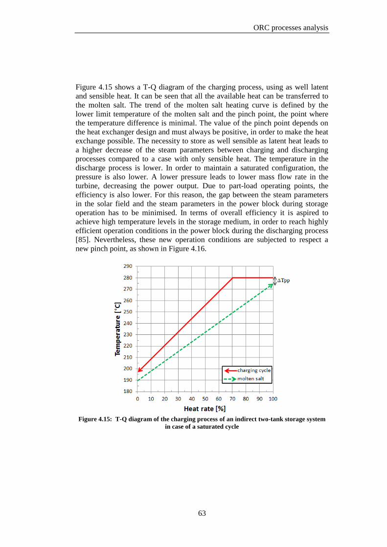
ORC processes analysis
63
Figure 4.15 shows a T-Q diagram of the charging process, using as well latent
and sensible heat. It can be seen that all the available heat can be transferred to
the molten salt. The trend of the molten salt heating curve is defined by the
lower limit temperature of the molten salt and the pinch point, the point where
the temperature difference is minimal. The value of the pinch point depends on
the heat exchanger design and must always be positive, in order to make the heat
exchange possible. The necessity to store as well sensible as latent heat leads to
a higher decrease of the steam parameters between charging and discharging
processes compared to a case with only sensible heat. The temperature in the
discharge process is lower. In order to maintain a saturated configuration, the
pressure is also lower. A lower pressure leads to lower mass flow rate in the
turbine, decreasing the power output. Due to part-load operating points, the
efficiency is also lower. For this reason, the gap between the steam parameters
in the solar field and the steam parameters in the power block during storage
operation has to be minimised. In terms of overall efficiency it is aspired to
achieve high temperature levels in the storage medium, in order to reach highly
efficient operation conditions in the power block during the discharging process
[85]. Nevertheless, these new operation conditions are subjected to respect a
new pinch point, as shown in Figure 4.16.
Figure 4.15: T-Q diagram of the charging process of an indirect two-tank storage system
in case of a saturated cycle

Chapter 4
64
Figure 4.16: T-Q diagram of the discharging process of an indirect two-tank storage
system in case of a saturated cycle
Figure 4.17 shows a configuration that couples a sensible heat with a latent heat
storage based on PCMs. During the charging process, heat from the condensing
steam is transferred to the melting PCM. During the discharging process, heat
from the solidifying PCM is used to generate steam. As represented in the T-Q
diagram of Figure 4.18, in these sections the temperature in the PCM remains
constant.
Figure 4.17: Integration of an indirect two-tank and a PCM storage system in a parabolic
trough power plant with saturated ORC direct steam generation
G

ORC processes analysis
65
Figure 4.18: T-Q diagram of the charging and discharging process of a PCM and indirect
two-tank storage system in case of a saturated cycle
In case of siloxanes the two phase-change is relatively small. Only a low amount
of the available heat from the ORC cycle can be utilized for PCM storage use.
Due to the limited experience in this temperature range and to the low thermal
conductivity in the solid phase, storage concepts with PCMs are still in
development to become cost-effective [86].
Supercritical cycle
In case of a supercritical cycle the only possible configuration is the indirect
two-tank molten salt storage system (Figure 4.19).
Figure 4.19: Integration of an indirect two-tank storage system in a parabolic trough
power plant with a supercritical ORC direct steam generation
G

Chapter 4
66
The T-Q diagram of the charging and discharging process is similar to the one in
case of saturated cycle. Due to the pinch-point limitation, the main difference is
that the supercritical cycle can obtain in the discharging process a better thermal
match with the heat source than the saturated one, as reported in Figure 4.20.
Hence, it can be noted that the gap between the steam parameters in the solar
field and the steam parameters in the power block during storage operation is
minimised.
Figure 4.20: T-Q diagram of the discharging process of an indirect two-tank storage
system in case of a supercritical cycle

67
5 Solar thermal ORC power plant
Modelization
In order to assess solar thermal ORC power plant configurations,
thermodynamic models in the simulation environment EBSILON®Professional
have been established. The plant model consists of three major components
which are described here in this chapter:
Solar field (SF)
Thermal Energy Storage System (TES)
Power block (PB)
The simulation study is perfomed for both the chosen cycle configurations of
Chapter 4 and is then divided into three phases:
1. Choice of the thermodynamic parameters of the cycle at design point;
2. Off-design analysis, which corresponds to the operating conditions
which vary from the nominal point at different DNI;
3. Evaluation of simulation data.
5.1 Preliminary Sizing
In the simulation of both cycles the solar field is assumed to be equal. The solar
field is characterized by its aperture area, type and number of collectors. In order
to determine the total aperture area and the number of collectors, a
preliminary sizing for an effective direct normal irradiation DNIeff of 850 W/m2
is made. The following assumptions are considered:
1. The chosen type of collectors is the Eurotrough ET150 with the Schott
receiver PTR70.
2. The proposed power plant is equipped with a TES system of 4 hours of full-
load capacity. Thus, the solar field compared to the power block must be
oversized. The solar multiple SM represents the solar field size related to the
power block, in terms of nominal thermal power. In this case a SM equal to
1.5 is fixed [87].
3. The gross electrical power of both plants is set to be 1 MWel, while

Chapter 5
68
the nominal cycle efficiency is assumed to be approximately 25%.
4. The nominal solar field efficiency is assumed to be equal to 75%. In
fact this value is overestimated in order to balance the assumed .
Table 5.1 summarizes the data used for the preliminary sizing.
Table 5.1: Assumed parameters for the sizing of both solar power plants
Parameters
Solar field technology Eurotrough ET150 +
Schott PTR 70
Thermal storage
capacity
4 h
1 MWel
25 %
1.5
850 W/m2
75 %
The sizing process is now described as follows.
The total aperture area is determined using the design-point power cycle rating,
the solar field efficiency and the desired solar multiple SM.
Since SM is defined as the ratio between the thermal power produced by the
solar field at the design point and the thermal power required by the
power block at nominal conditions
(5.1)
the solar field thermal output at design is calculated according to the
following equation
(5.2)
Hence, the total incident thermal energy can be determined by dividing
the total thermal energy output by the solar field efficiency, as shown in
Equation (5.3).

Solar thermal ORC power plant Modelization
69
(5.3)
Therefore, the effective aperture area is given by
(5.4)
Therefore, the effective number of collectors is calculated by
(5.5)
By rounding off this value and estimating to an even number so as to obtain the
symmetry of the collectors in each loop, the chosen number of collectors is
equal to 12. In all, the gross aperture area is 10386 m².
5.2 EBSILON®Professional
The software used in this thesis to model the solar thermal power plant and to
run thermodynamic calculation on the cycle conditions is
EBSILON®Professional 10.05 (referred to as EBSILON in this thesis), a
commercial simulation software developed by STEAG Energy Services GmbH.
EBSILON is the abbreviation for “energy balance and simulation of the load
response of power generating or process controlling network structures”. It is a
Windows-based modeling tool with a graphical user interface that allows the
drag-and-drop arrangement of multiple pre-built components connected by
material and logic lines to simulate thermodynamic cycle processes for power
plants in the steady state.
As shown in Figure 5.1, the basic control elements and tool bars are:
Standard toolbar
Component bar, for selecting a component from a category
Component wizard bar, for accessing components classified by numbers
Ebsilon bar, for starting simulations
Zoom bar, for zooming in the model and finding objects

Chapter 5
70
Figure 5.1: EBSILON control elements and tool bars
After defining the design of the cycle, it is necessary to define the values that
characterize it. There are two ways of doing that:
1. Some components can be defined directly in their component properties
window, like e.g. the Sun (Component 117), as shown in Figure 5.2
2. The other possibility is to set a value (e.g. mass flow, temperature or
pressure) directly on a pipe of the cycle using the "Measured/General
value input" (Component 46 or 33), as shown in Figure 5.3.
Figure 5.2: Defining data of a component in EBSILON

Solar thermal ORC power plant Modelization
71
Figure 5.3: Defining data of a pipe in EBSILON
A variety of fluids, such as water, gases, heat transfer fluids, and combustibles
are implemented in EBSILON. Additionally, fluid properties from the
REFPROP library, distributed by NIST [88], can be used. The present thesis
makes use of the fluid properties of the siloxanes MM and D4.
Only if all necessary values have been supplied, and the system is completely
determined, a power plant process simulation can be successfully computed.
EBSILON is composed of two calculation modes:
• Design Calculation ("full load")
• Off-design Calculation ("part load")
In the design mode, the calculation runs using the user defined specification
values for all components for a nominal operating point in order to store the
results as reference values for off-design and allow the components to be sized.
In off-design mode components are then fixed and simulations can be performed
for different sets of input data. In all standard EBSILON components
correlations for the calculation of off-design operating-points are implemented.
EBSILON offers the possibility of handling different cycle cases in "profiles" in
a tree-like hierarchy. Profiles help the user to manage several variations of one
cycle within one document. This is especially useful for handling design and
off-design calculations as well as property data variation. The root of this tree is
always the design case. An example of such a hierarchy scheme is shown in
Figure 5.4.

Chapter 5
72
Figure 5.4: Hierarchy tree in EBSILON
The subprofiles inherit all properties, such as the specification values and
characteristics of all components, from its parent. In this thesis the parent profile
is always the design case, so that nearly all parameters values are assigned in the
root profile. In the respective subprofiles the analysed parameter (e.g. DNI) and
the operational parameters can be defined or changed in order to meet the plant
control strategies.
5.3 Solar field
The modeling of the main components of the solar field (e.g. the sun, line
focusing collectors, piping and headers) is carried out taking advantage of the
add-on EbsSolar library [89], developed in cooperation with the DLR.
5.3.1 The sun
In EBSILON, the sun is represented by Component 117. According to
DIN 5034 [90], the solar azimuth ( ) and solar height angle ( ), both shown in
Figure 5.5, are calculated using the inputs of local time, latitude, and longitude.
Assuming that the PTC is not built on a slope and the collector axis is oriented
north-south ( = 0), the tracking angle ( ) and the incident angle ( ) can be
calculated with equations (5.6) and (5.7).
(5.6)
√
(5.7)

Solar thermal ORC power plant Modelization
73
Figure 5.5: The angles of a parabolic trough collector in relation to the sun adapted from
[91]
5.3.2 Parabolic trough collector
For the simulation the EuroTrough collector with the Schott PTR70 receiver has
been chosen. The selected PTC is modelled in EBSILON by Component 113,
represented in Figure 5.6. Equations for heat balance and pressures drops are
implemented in this component and are described in detail in the following
subsections.
Figure 5.6: Representation of the parabolic trough collector model in EBSILON
Heat balance
The effective heat transferred to the fluid flow is calculated by the difference
between the incoming optical thermal power and the total heat losses that
occur in the receiver , as shown in Equation (5.8).

Chapter 5
74
( ) ( ) (5.8)
with:
- : optical peak efficiency;
- : reflecting mirror cleanliness factor;
- : shading loss factor;
- : end loss factor;
- ( ) : incident angle modifier as a function of in degree;
- : focusing state of the collector;
- : thermal losses of the receiver.
In the simulation of on-design conditions (with incidence angle set to 0°),
and are set respectively to 0.75 and 1 [87]. For a further explanation of
these efficiency factors see Appendix. With an incidence angle of 0°, reciprocal
shading effect and endlosses effect do not occur.
The incident angle modifier ( ) accounts for optical losses and spillage of
solar radiation with increasing incident angle. The is described by a
second-order polynomial correlation:
( ) ( (
)) (5.9)
where and are two empiric parameters. The measured parameters of the
EuroTrough collector are the following [92]:
= 0.00010596;
= -0.00017091.
Figure 5.7 shows the graphical representation of the IAM correlation.

Solar thermal ORC power plant Modelization
75
Figure 5.7: IAM correlation of the Eurotrough collector
The focusing state of the collector ( ) is a parameter that simulates the
defocusing of the PTCs. It can assumed a value between 0 and 1, with 0 being a
completely defocused state and 1 being normal.
The total heat losses in the receiver are due to convection, radiation and
conduction in and around the receiver, as shown in Figure 5.8 [93]. In order to
specify all the heat transfers, the nomenclature is specified in Table 5.2.
Figure 5.8: One-dimensional heat balance of a receiver [91]
0
0,1
0,2
0,3
0,4
0,5
0,6
0,7
0,8
0,9
1
0 10 20 30 40 50 60 70 80 90
IAM
, co
s(θ
i)
Incidence angle θi [°]
cos(θi)
IAM
IAM∙cos(θi)
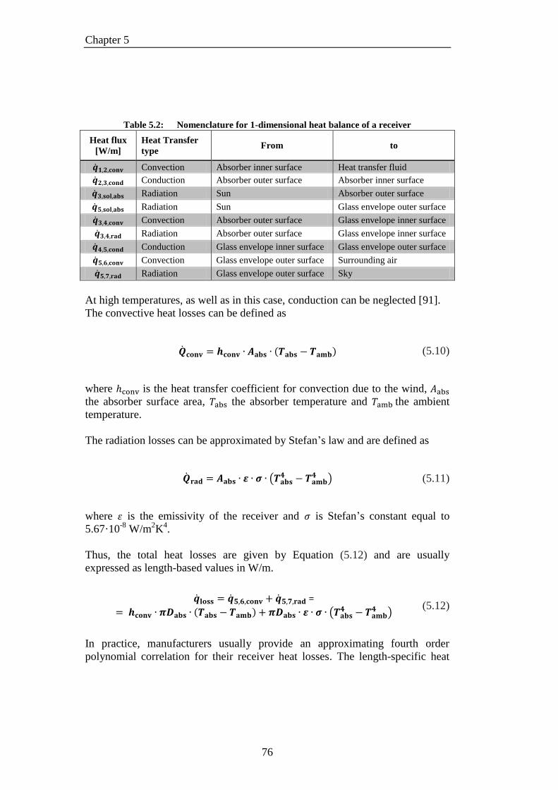
Chapter 5
76
Table 5.2: Nomenclature for 1-dimensional heat balance of a receiver
Heat flux
[W/m]
Heat Transfer
type From to
Convection Absorber inner surface Heat transfer fluid
Conduction Absorber outer surface Absorber inner surface
Radiation Sun Absorber outer surface
Radiation Sun Glass envelope outer surface
Convection Absorber outer surface Glass envelope inner surface
Radiation Absorber outer surface Glass envelope inner surface
Conduction Glass envelope inner surface Glass envelope outer surface
Convection Glass envelope outer surface Surrounding air
Radiation Glass envelope outer surface Sky
At high temperatures, as well as in this case, conduction can be neglected [91].
The convective heat losses can be defined as
( ) (5.10)
where is the heat transfer coefficient for convection due to the wind,
the absorber surface area, the absorber temperature and the ambient
temperature.
The radiation losses can be approximated by Stefan’s law and are defined as
(
) (5.11)
where is the emissivity of the receiver and is Stefan’s constant equal to
5.67·10-8
W/m2K
4.
Thus, the total heat losses are given by Equation (5.12) and are usually
expressed as length-based values in W/m.
=
( ) (
) (5.12)
In practice, manufacturers usually provide an approximating fourth order
polynomial correlation for their receiver heat losses. The length-specific heat
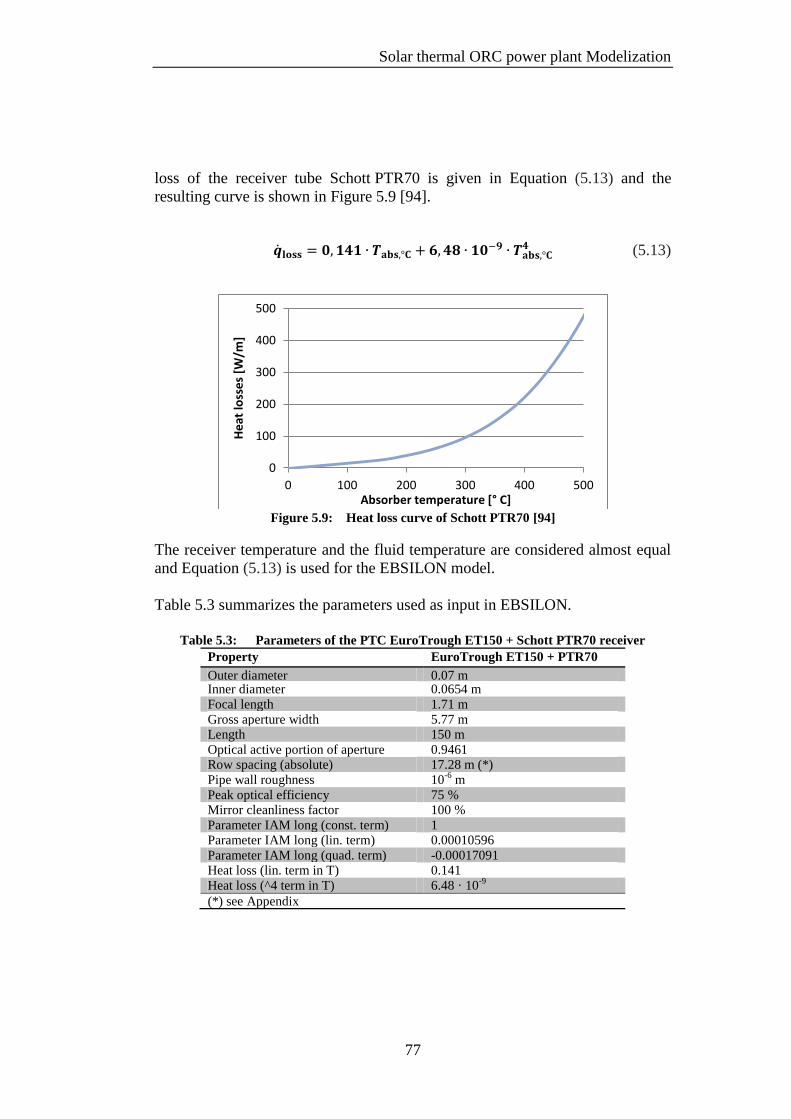
Solar thermal ORC power plant Modelization
77
loss of the receiver tube Schott PTR70 is given in Equation (5.13) and the
resulting curve is shown in Figure 5.9 [94].
(5.13)
Figure 5.9: Heat loss curve of Schott PTR70 [94]
The receiver temperature and the fluid temperature are considered almost equal
and Equation (5.13) is used for the EBSILON model.
Table 5.3 summarizes the parameters used as input in EBSILON.
Table 5.3: Parameters of the PTC EuroTrough ET150 + Schott PTR70 receiver
Property EuroTrough ET150 + PTR70
Outer diameter 0.07 m Inner diameter 0.0654 m
Focal length 1.71 m
Gross aperture width 5.77 m Length 150 m
Optical active portion of aperture 0.9461 Row spacing (absolute) 17.28 m (*)
Pipe wall roughness 10-6
m
Peak optical efficiency 75 % Mirror cleanliness factor 100 %
Parameter IAM long (const. term) 1 Parameter IAM long (lin. term) 0.00010596
Parameter IAM long (quad. term) -0.00017091 Heat loss (lin. term in T) 0.141
Heat loss (^4 term in T) 6.48 · 10-9
(*) see Appendix
0
100
200
300
400
500
0 100 200 300 400 500
He
at lo
sse
s [W
/m]
Absorber temperature [° C]

Chapter 5
78
Pressure drops
Pressure drops that occur in the absorber tube of the collector are composed of
two parts, the frictional pressure drops and the momentum pressure drops
(acceleration) .
(5.14)
Both pressure drops are calculated based on state-of-the-art correlations already
implemented in EBSILON. The correlations used differ depending on whether
the flow is single-phase or two-phase.
For a single-phase flow, the frictional pressure drop is calculated with the
Darcy-Weisbach equation (5.15), with the coefficient of friction determined in
case of turbulent flow by the Colebrook equation (5.16):
(5.15)
with
√ (
√ ) (5.16)
(5.17)
where:
: coefficient of friction
: Reynolds number
: absorber pipe inner diameter (m)
: absolute internal pipe roughness (m)
: mean density (kg/m3)
: mean velocity (m/s)
The momentum pressure drop reflects the change in kinetic energy of the flow
and is calculated for a single-phase flow according to Equation (5.18).

Solar thermal ORC power plant Modelization
79
(5.18)
Two-phase pressure drops, as needed for direct steam generation applications,
can be calculated with the empirical correlation of Friedel [95]. This correlation
is also implemented in the collector models in EBSILON.
In order to evaluate the two-phase frictional pressure drop, the single liquid-
phase pressure drop is multiplied with a two-phase multiplier [25]:
(5.19)
The two-phase multiplier is calculated by Equation (5.20), which is valid for
viscosity ratios of
1500.
( )
( )
( )
(
)
(
)
(5.20)
where:
: vapor quality
: coefficient of friction for the singles gas-phase
: coefficient of friction for the single liquid-phase
Weber and Froude number are calculated as follows:
(5.21)
(5.22)
where:
: surface tension (N/m)
: gravitational acceleration (m/s2)

Chapter 5
80
The two-phase momentum pressure drop is given by
{[
( )
( )
]
[( )
( )
]
} (5.23)
where is the mass velocity (kg/m2s) and is the void fraction calculated as
follows:
[( ( ))(
)
( )[ ( ]
]
(5.24)
5.3.3 Layout
The solar field consists of:
- A cold distributing header, where the mass flow coming from the power
block is split into several collector loops;
- A number of loops consisting of 2 or more PTCs connected in series
trough a “U” configuration;
- A hot collecting header, that collects the fluid from the loops to the
power block.
The solar field can be arranged in different layouts. For traditional solar thermal
plants working with HTF, two field layouts are usually adopted: an ‘H’ field
layout for collector field areas greater than 400000 m2, and an ‘I’ field layout for
areas less than 400000 m2 [96]. Other layouts have been proposed for specific
class of power plant. As shown in Figure 5.10, the chosen solar field’s layout for
the small-scale DSG-ORC power plant consists of 6 collector loops, each
consisting of 2 Eurotrough ET150 collectors.
In order to minimize the mutual shading phenomenon (Appendix) and to ensure
accessibility to the collector loops, an optimum value for the distance between
the rows of collectors ( ) is used. A trade-off between land-use and shading
phenomenon suggests adopting a value equal to approximately 3 times the
collector width [91]. According to state-of-the-art row distance, a value of
17.28 m has been set.

Solar thermal ORC power plant Modelization
81
Figure 5.10: Solar field layout, consisting of 6 collector loops with 2 collectors per loop
In case of the saturated configuration, the recirculation mode is applied. For
compact water-steam separators in DSG systems, the inlet steam quality is
normally set between 0.7-0.8 [26]. In this case the two-phase flow exits the solar
field with an imposed vapor quality x of 0.5 [87], in order to be more
conservative. Downstream of the solar field, the liquid phase is separated and
recirculated while saturated steam (with x = 1) is flows to the turbine.
The simulation in EBSILON models only one representative PTC loop. Thus, in
order to consider the whole solar field, the mass flow rate of the fluid is
increased by a factor of six after the loop.
Piping and headers
As mentioned before, headers are installed for distributing and collecting the
working fluid in the collector field. In both headers heat and pressure losses
occur.
In order to identify the piping heat losses, a heat loss factor of 10 W/m2
found in literature [97] has been used. The total heat losses of headers and
piping are then calculated according to Equation (5.25).
(5.25)

Chapter 5
82
In order to identify the piping pressure drop, the pressure drop in the flow to the
outermost loop should be calculated. In fact, it defines the pressure drop in the
flows through all of the loops. The pressure drop in the inner loops is set equal
to the pressure drop in the last loop by the throttling action of valves in the inner
loops. A simplified scheme of this hydraulic analysis is represented in Figure
5.11.
Figure 5.11: Simplified scheme of hydraulic analysis pipe network
In order to approximate the frictional pressure drop, the correlations described
previously for the collector are still valid and a simple model has been run in
EBSILON. Firstly, lengths and inner diameters of both header pipes have to be
sized. Referring to Figure 5.10, the total length of one header ( ) depends on
the number of branches ( ), on the row distance between the collectors ( )
and on the distance from the PB to the first loop ( ):
( ) (5.26)
The chosen sizing for the inner diameter is based on maintaining constant the
fluid velocity along the pipe length. This characteristic involves a theoretical
pipe diameter modification every time the mass flow changes. Cold header pipe
diameter decreases as the distance from the power block increases (Figure 5.12),
whereas hot header pipe diameter increases as the distance to the power block
decreases.

Solar thermal ORC power plant Modelization
83
Figure 5.12: Schematic representation of a cold header
In order to determine the optimum diameter of each header section, the design
velocity has been set to 2 m/s for the liquid flow in the cold heater and to 10 m/s
for the vapour flow in the hot header [87]. Once the diameters are selected, the
frictional pressure drops are carried out.
Hence, the total pressure drops for both configurations can be calculated for
each header. For simplicity, pressure drops through the pipe fittings (e.g. elbows
or tees) are neglected.
5.4 Thermal storage system
The thermal storage system consists of a hot and a cold tank. In respect of the
temperature range of the cycle (195°C-280°C), and of its availability in
EBSILON, the chosen storage media is HITEC molten salt. Its characteristics
are compared with the ones of the thermal oil and other types of molten salt in
Table 5.4.
Table 5.4: Molten salt and Therminol VP-1 properties
Salt Solar Salt HITEC HITEC XL Therminol VP-1
Composition (%) biphenyl/diphenyl
NaNO3
KNO3
NaNO2
Ca(NO3)2
60
40
7
53
40
7
45
48
Maximum temperature (°C)
Melting temperature (°C)
Density @ 300°C (kg/m3)
Heat capacity @ 300°C (J/kgK)
600
220
1899.2
1391.4
535
142
1864.8
1561.7
500
120
1992
1447
400
13
815
2319
Nominal cost ($/kg) 0.49 0.93 1.19 2.2
The thermal storage system is then modelled using a simple energy balance
approach that includes charging and discharging energy rates, thermal losses and

Chapter 5
84
general sizing inputs. As shown in Figure 5.13, the solar field circuit and the
storage tank circuit are connected with a heat exchanger. Component 118
represents a tank equipped with two connections, one for an inflow and one for
an outflow. The concept of two connections is chosen, because in EBSILON
modeling flow reversal is not feasible. In EBSILON the storage model itself is
not responsible for keeping the load state within tolerated limits “empty” or
“full”. This task as well as supervising consistence with minimum and
maximum mass flow rates during charge or discharge operation has to be solved
by use of control or limiter components.
Figure 5.13: Representation of the indirect two-tank storage system in EBSILON
The organic working fluid in both cycle configurations leaves the solar field at
approximately 280°C and is then pumped directly to the turbine or, in storage
system charging mode, to the heat exchanger. There, the HITEC solar salt
coming from the cold tank at (190°C) is heated up to (275°C),
the design temperature level of the hot tank. The design temperature value of the
cold tank is chosen in order to avoid the melting temperature of the salt, while
the one of the hot tank in order to ensure a of 5°C during the charging
process. Hence, for storage system charging mode, three temperature boundary
conditions are already given. The remaining free variable is either the organic
working fluid outlet temperature or one of the two fluid mass flow rates. In this
study the design mass flow rate of the organic fluid in charging mode is
assumed to be approximately 8.44 kg/s in case of D4 and 8.53 kg/s in case of
MM. The corresponding mass flow rate of the molten salt and the organic fluid
outlet temperature (solar field return temperature) is calculated for steady state.
For storage system discharging mode, the HITEC salt feed and drain
temperatures are given as well. Here, the hot salt at 275°C is pumped from the

Solar thermal ORC power plant Modelization
85
hot tank, through the heat exchanger, and fed into the cold tank at 190°C. The
organic fluid inlet temperature corresponds to the regenerator exit temperature.
The remaining free variable is either the organic fluid outlet temperature or one
of the two fluid mass flow rates. In contrast with the charging mode, this kind of
approach is valid only in case of MM (supercritical cycle). Here, the HITEC
mass flow rate is set and the corresponding mass flow rate of the organic fluid
and its outlet temperature (turbine inlet temperature) are calculated for steady
state. In case of D4, due to the saturated cycle configuration, remaining free
variables are not allowed and only one possible charging mode exists. As we
will see in next chapter, this charging mode has to be determined performing a
pinch-point analysis in the heat exchanger. Figure 5.14 shows a simplified
scheme of the charging and discharging modes in an indirect two-tank storage
system.
Figure 5.14: Scheme of charging and discharging modes in an indirect two-tank storage
system adapted from [91]
The thermal capacity of the storage is evaluated with Equation (5.27), assuming
4 hours of full-load operation (power block in storage-only mode).
( ) (5.27)
where
is the discharge efficiency due to the heat losses in the heat
exchangers.
T3T4

Chapter 5
86
Each storage tank has the same volume calculated as follow
(5.28)
The evaluated tank capacity is then increased taking into account the thermal
losses and a security gap.
In this study the dependence of the heat losses from the salt temperature and
from the fill level of each tank has been neglected. Heat losses are
expressed as function of the capacity with an empiric factor a:
(5.29)
A maximal heat loss of 1% of the storage capacity per 12 hours corresponds to
an a value of 2.3148∙10-11
1/s [91].
Table 5.5 summarizes the specific data of the storage system used as input in
EBSILON. Pressure drops in the heat exchangers are neglected.
Table 5.5: Specific data of the TES system used in EBSILON
Cold TES Hot TES
Diameter 9.5 m 9.5 m
Height 3.5 m 3.5 m
Mass at full state 460 t 460 t
Temperature in storage 190°C 275°C
Pressure in storage 1.5 bar 1.5 bar
5.5 Power block
As mentioned before, the PB’s gross electrical power is approximately 1 MW,
and a turbine inlet temperature of 280°C is chosen for both the saturated and the
supercritical cycles. For the construction of the PB in EBSILON, proper
components available in its standard library have been selected. All the data
assumed to characterize each component are reported in details in the following
sub-sections, while the equations to define their performances can be found in
Chapter 4, Section 4.2.

Solar thermal ORC power plant Modelization
87
5.5.1 ORC Turbine
The ORC turbine is designed with Component 6 (Figure 5.15) and is then
connected to a generator (Component 11) with a generator efficiency of
0.96. In nominal conditions, the turbine is defined by several parameters as the
isentropic efficiency ( = 0.83) and the mechanical efficiency ( = 0.998)
[98]. The nominal inlet pressure is set by using a “general input value” in
accordance with the chosen values.
For the supercritical cycle, the value of the turbine inlet pressure has been
analysed from a thermodynamic point of view in Chapter 4. Even if a value
close to the critical pressure leads to slightly higher cycle performances, in the
simulation model a higher pressure value is used. As explained further, in this
case a turbine inlet pressure of 30 bar is used in order to avoid the two-phase
region in off-design mode.
Figure 5.15: Representation of the turbine in EBSILON
In order to perform off-design simulations, the turbine operates usually in
sliding pressure (see Section 6.2) following the Stodola’s Cone Law [99]. Once
the design parameters are given, the law determines the relationship between the
turbine inlet and outlet pressure and the mass flow through the turbine.
Figure 5.16 shows this dependence in a 3-dimensional diagram that has the
shape of a degenerate quadric surface, the cone directrix being an ellipse.

Chapter 5
88
Figure 5.16: Graphic representation of Stodola's cone law
Considering an ideal gas, the Stodola’s Cone law equation can be simplified to
[100]:
√
(
)
(
) √
(5.30)
where “ ” is the mass flow rate, “ ” the pressure and “ ” the temperature in the
turbine respectively. The sub-index “in” stands for the inlet value, “out” for the
outlet value and “N” for the design values.
Thus, from a given mass flow the corresponding turbine inlet pressure required
by the turbine nozzle area can be calculated in according to Equation (5.31):
√ (
)
(
)
(5.31)
The other important parameter that changes when simulating in off-design
conditions is the turbine isentropic efficiency . In fact, it is influenced by
many design parameters as blade construction and operation points, reaching its
maximum value at full load. Most of the documentation available refers as
a function of the ratio between the actual enthalpy drop and the design enthalpy
drop, in accordance with [101]. In EBSILON such a function could not be
implemented. Hence, the final solution was adapting it as a function of the
mass/volume flow rate.

Solar thermal ORC power plant Modelization
89
5.5.2 Regenerator
Component 26 is used to model a regenerator that operates in counter-current
flow without pressure drops. In design mode, the cycle parameters are set in
order to permit the calculation of the proper T2 and T4 (indicated in Figure 5.17)
by the component using an effectiveness of 0.9 [102].
(5.32)
Figure 5.17: Representation of the regenerator in EBSILON
The total UA parameter, which gives a reasonable indication of the heat
exchanger dimension, is calculated according to the following formula:
(5.33)
where is the logarithmic mean temperature difference defined as
(5.34)
with
(5.35)
(5.36)

Chapter 5
90
In off-design mode, it is assumed that the performance of the component (i.e.
UA as a function of other influencing parameters) is known and is either
specified as a characteristic line.
5.5.3 Condenser and cooling system
Condensers operate by removing heat from a vapor to a liquid state. The three
main types used in power plants are water-cooled condensers, cooling towers
and air-cooled condensers.
- In the first type of condensers, the steam flow is sent to a heat exchanger
in which the condensation occurs using cooling water as a refrigerant
fluid. The cooling water can be provided from a river or the sea, from
where it is pumped to the condenser. The condenser consists of a pipe
bundle through which the cooling water is heated while the steam
outside the pipes is condensed. These condensers are realized as shell-
and-tube or tube-and-tube type. The application of this type of condenser
is limited to those facilities that have easy access to water sources.
Therefore they are not recommended for CSP applications that are
normally built in desert areas.
- Cooling towers are heat exchangers in which two fluids, water and
cooling air, are put in contact to transfer heat. The cooling is therefore
possible through the exchange of heat and mass between the two fluids.
There are two main types of cooling towers: open circuit and closed
circuit. In an open circuit the hot water from the condenser is sprayed
into a rain-like pattern, through which the ambient air is induced directly
by fans. A closed circuit works through the same physical principle of
heat exchange, but without a direct contact between the condensing
water and the air. Cooling towers are the most used types of condensers
in large-scale CSP plants.
- Air-cooled condensers are used in places where it is difficult to find a
source of cooling water. In this case the steam flow is condensed into
thinned tubes by ambient air moved by axial fans. One of the
disadvantages of this type of condenser is that the heat transfer
coefficient of the air is substantially lower than that of water, and, in
order to improve the heat exchange, there is the need to increase the
surface area of the condenser. In addition, the dry-bulb temperature is
higher than the wet-bulb one. Thus, in comparison with cooling towers,
air coolers reject heat at a higher temperature. Although air-cooled
condensers require less maintenance, they produce more noise, as well as

Solar thermal ORC power plant Modelization
91
power consumption, due to the air exchange forced by fans. The growing
attention to minimize the consumption of water makes this type of
condensers an attractive option for CSP plants (e.g. Ivanpah plant [11]).
Therefore, in case of the supercritical configuration with MM, an air-cooled
condenser is chosen and it is modeled in EBSILON with Component 7 (Figure
5.18). Pressure drops in this component are neglected.
Figure 5.18: Representation of the air-cooled condenser in EBSILON
The amount of steam to be condensed, the steam enthalpy, the air inlet
temperature and its pressure are specified. In design mode, the temperature rise
of the cooling air is provided, giving as input the air inlet temperature ,
the approach-point and the pinch-point (Table 5.6). EBSILON then
calculates the nominal cooling air flow rate and the nominal value for UA. The
UA-value of the off-design calculation results from the UA-value of the design
calculation multiplied by a correction factor that is determined by a default
characteristic line. In case the cooling air outlet temperature is specified,
EBSILON then calculates a new value for the cooling air flow rate. In this
model heat losses to the surroundings are not taking into account.
Table 5.6: Parameters for the calculation of the temperature rise in the condenser
30°C
15°C
1°C
As analysed in Chapter 4, the desired condensing pressure should not be lower
than 0.05 bar. In case of the fluid D4, this leads to a relatively high condensing
temperature (87.3°C). In order to take advantage of the heat reject at this
condensing temperature (e.g. absorption chillers), for the saturated cycle with
D4, the condenser is replaced with a Heat Consumer (Component 35 in Figure
5.19).

Chapter 5
92
Figure 5.19: Representation of the heat consumer in EBSILON
5.5.4 Pump
The task of the pump is to raise the pressure of the fluid from a low to a high
value. In EBSILON, Component 83 (represented in Figure 5.20) is used to
model a multistage centrifugal pump with variable speed. A nominal hydraulic
efficiency of 0.7 [98] and a mechanical efficiency of 0.998 are
defined. In fact, the model calculates the enthalpy at the outlet, based on this
efficiency, with the volume flow and pressure head being imposed by measuring
points at the inlet and outlet of the pump. The pump is then coupled with a
motor (Component 29), characterized by a nominal electrical efficiency of
0.85.
In both configurations two pumps are normally used: one condensate pump and
one feed pump before the solar field. Due to the recirculation mode, in case of
the saturated configuration, an extra recirculation pump is used. All of them
have the same assumed parameters.
In off-design mode the performance of each pump is given by an efficiency
characteristic line already implemented in EBSILON.
Figure 5.20: Representation of the pump in EBSILON

Solar thermal ORC power plant Modelization
93
5.6 Reference systems
As mentioned in the previous sections, both power plant configurations consists
of 6 collector loops of the model Eurotrough ET150 with a total net collector
area of 9826 m2. The storage capacity sums up to 4 full load hours.
The most important technical parameters are summarized in Table 5.7.
Table 5.7: Technical specifications of the reference systems
Description Symbol
Supercritical
configuration
with MM
Saturated
configuration
with D4
Parameters for solar field and storage system
Solar multiple 1.5
Gross aperture area of the solar field 10386 m2
Net aperture area of the solar field 9826 m2
Number of full load hours in storage 4 h
Storage capacity 16 MWh
Storage efficiency charging and
discharging 95%
Parameters for the PB at design point
Turbine inlet temperature 280°C
Turbine inlet pressure 8.076 bar 30 bar
Isentropic turbine efficiency 83%
Generator efficiency 96%
Regenerator effectiveness 90%
Isentropic pump efficiency 70%
Motor pump efficiency 85%
Condensing pressure 0.141 bar
(Air-coolers)
0.05 bar
(CHP)
5.7 Simulation layouts
In Figure 5.21 and Figure 5.22 the simulation layout for both configurations is
presented as displayed in EBSILON. The plant operates as follows. The cold
liquid at the solar field inlet (state 3) is heated by the solar field to state 4. Here,
a part of the hot fluid enters the TES system circuit, while the remaining fraction
is sent to the PB. Both streams are then mixed up again before the feed pump.
It must be noted, that the specific properties of the chosen ORC fluids lead to
numerical instabilities in EBSILON. Therefore, in order to make the simulations
successfully converge, some pipes in the layout model are physically decoupled.
For simplicity, in these cases the boundary conditions have been set properly on
the pipes using transmitter elements.
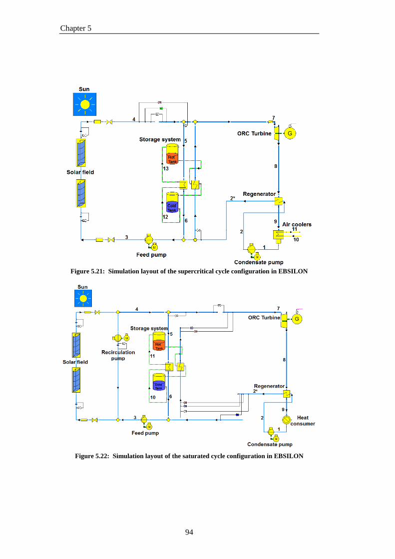
Chapter 5
94
Figure 5.21: Simulation layout of the supercritical cycle configuration in EBSILON
Figure 5.22: Simulation layout of the saturated cycle configuration in EBSILON

Solar thermal ORC power plant Modelization
95
A simulation has been run for both configurations in order to assess how the
whole system works under nominal conditions, thus with a of 850 W/m2.
For each cycle point the following data are carried out. Table 5.8 refers to the
supercritical configuration (MM), while Table 5.9 to the saturated one (D4).
Table 5.8: Cycle parameters obtained in EBSILON at nominal conditions for the
supercritical configuration
Point Fluid (kg/s)
T
(°C)
p
(bar)
h
(kJ/kg)
s
(kJ/kgK)
1 MM 12.1 44.9 0.141 -112.128 -0.324
2 MM 12.1 46.7 30 -106.381 -0.319
2* MM 12.1 152 30 113.432 0.273
3 MM 20.6 170.6 34.654 155.479 0.368
4 MM 20.6 280 30 452.75 0.963
5 MM 8.5 280 30 452.75 0.963
6 MM 8.5 195 30 212.49 0.495
7 MM 12.1 280 30 452.75 0.963
8 MM 12.1 187.2 0.141 355.608 1.001
9 MM 12.1 62.4 0.141 135.795 0.453
10 AIR 189.8 30 1 30.155 6.885
11 AIR 189.8 45.7 0.99875 45.963 6.936
12 HITEC salt 15.4 190 1 296.719 0.825
13 HITEC salt 15.4 275 1 429.461 1.088
Table 5.9: Cycle parameters obtained in EBSILON at nominal conditions for the
saturated configuration
Point Fluid (kg/s)
T
(°C)
p
(bar)
h
(kJ/kg)
s
(kJ/kgK)
1 D4 17.1 87.3 0.05 -152.838 -0.378
2 D4 17.1 87.9 8.076 -151.524 -0.377
2* D4 17.1 195.9 8.076 38.59 0.082
3 D4 25.6 196.4 16.104 39.546 0.082
4 D4 25.6 280 8.076 280.785 0.545
5 D4 8.4 280 8.076 280.785 0.545
6 D4 8.4 195 8.076 36.810 0.078
7 D4 17.1 280 8.076 280.785 0.545
8 D4 17.1 231.1 0.05 223.345 0.569
9 D4 17.1 104 0.05 33.231 0.137
10 HITEC salt 15.5 190 1 296.719 0.825
11 HITEC salt 15.5 275 1 429.461 1.088

Chapter 5
96
5.8 Plant operation management
The advantage of a CSP power plant coupled with a TES system is the ability to
store heat energy for short periods of time and thus have a “buffering” capacity
that allows it to smooth electricity production considerably.
Various plant operation modes can be outlined. For instance, the system may
operate according to the following operation modes:
1. Start and stand-by operation mode;
2. Solar operation and charging mode;
3. Defocus mode;
4. Solar operation and discharging mode;
5. Storage-only operation mode.
5.8.1 Start and stand-by operation mode
The start and stand-by operation is a solar part-load operation that occurs when
the solar irradiation is not high enough to run the power block at full load (e.g.
in the early morning) and the storage system is empty (Figure 5.23). According
to the chosen control logic, the outlet field temperature is maintained fixed at the
design vaue of 280°C. Thus, a lower mass flow rate is heated up. The solar field
provides all the thermal energy directly to the PB, avoiding the accumulation
phase in the storage system.
Figure 5.23: Simplified representation of the start and stand-by operation mode
Turbine G
Hot tank
Power blockStorage-SystemSolar field
Cold tank

Solar thermal ORC power plant Modelization
97
5.8.2 Solar operation and charging mode
The middle of the day, especially during summer, is usually characterized by
high DNI values. Here, the solar field can provide a thermal energy to the PB
even higher than that required to run it at full load. In this case the heat rate in
excess is stored in the TES system. As shown in Figure 5.24, the fluid passes
through a heat exchanger in the TES circuit and transfers its heat to the molten
salt. The molten salt is pumped from one tank to another, from a temperature of
190°C to 275°C. To ensure reliable operation of the heat exchanger a margin on
the minimum mass flow rates that flow in the heat exchanger should be set.
Thus, the inlet temperature to the SF is given by mixing the fluid coming from
the heat exchanger of the storage system with the fluid coming from the PB
(regenerator outlet).
Figure 5.24: Simplified representation of the solar operation and charging mode
5.8.3 Defocus mode
As explained in Section 5.1, the solar thermal ORC plant has been sized with a
DNIeff of 850 W/m2. When the effective DNI exceeds the design value, there is
an overproduction of heat in the solar field. According to the adopted control
strategy, the mass flow rate of the organic fluid is greater than that produced in
nominal conditions. Hence, when the storage system is full, the turbine capacity
increases. Some collectors must be defocussed in order to avoid that the
Turbine G
Hot tank
Power blockStorage-SystemSolar field
Cold tank

Chapter 5
98
maximum turbine capacity is exceeded (in our case 110% of the design
capacity). This value represents a limit for the operation of the turbine.
5.8.4 Solar operation and discharging mode
This mode of operation provides the simultaneously generation phase from both
the SF and the TES system (Figure 5.25). It occurs during the day when the
thermal energy produced by the SF is not sufficient to meet the electricity
demand and, therefore, must be complemented by taking the portion missing
from the TES system. Part of the fluid from the regenerator passes through the
TES system circuit and is heated in the heat exchanger, while the other passes in
the SF. Both flows have a significant pressure difference depending on the
operating points. To mix up both flows together in front of the turbine, the
pressure of the stream from the solar field has to be throttled in order to be at
least equal to the storage discharge pressure. Hence, if stream is taken from both
the solar field and the storage, the system operates in sliding pressure mode. Due
to this mode, with this plant configuration the design power cannot be
maintained during long low-irradiance periods by means of the storage.
Figure 5.25: Simplified representation of solar operation and discharging mode
Turbine G
Power blockStorage-SystemSolar field
Cold tank
Hot tank

Solar thermal ORC power plant Modelization
99
5.8.5 Storage-only operation mode
The storage-only operation mode may be perfomed during bad weather periods
or during the night. Here, only the stored heat from the TES system is used to
operate the ORC cycle (Figure 5.26). The discharging process of the TES
system should be represented in a T-Q diagram in order to evaluate the
feasibility of the heat exchange in accordance with the preliminary study
conducted in Chapter 4, Section 4.5. It is important to remember that a main
difference arises in the heat exchange when using a supercritical configuration
instead of a saturated one, as a consequence of the different thermal match in the
heat exchanger.
Figure 5.26: Simplified representation of storage-only operation mode
Turbine G
Power blockStorage-SystemSolar field
Cold tank
Hot tank

Chapter 5
100

101
6 Evaluation of simulation data
In order to characterize the performance of the systems in design, off-design and
storage-only operation modes, the net electric power and the system efficiencies
are carried out. The net electric power of the PB is defined as follows:
(6.1)
where:
is the gross electrical power calculated by multiplying the mechanical
turbine power by the generator efficiency .
(6.2)
is the parasitic power that includes the electricity of the following
consumers:
- Condenser fan (only in supercritical configuration, as explained in
Section 5.5.3)
(6.3)
with:
: air pressure drop, assumed to be equal to 125 Pa;
: fan total efficiency, assumed to be equal to 0.8 [98].
- Condensate pump (CP)
( )
(6.4)
- Feed pump before the solar field (FP)
( )
(6.5)

Chapter 6
102
- Recirculation pump (only in saturated configuration) (RP)
( )
(6.6)
The thermal efficiency of the cycles was already defined in Chapter 4. It is
important to highlight here that this cycle efficiency cannot provide accurate
informations about the whole system plant, since it is referred only to the PB
without considering the contribution of all the parasitic consumers. In case of a
solar thermal power plant, the thermal efficiency should be redefined as
(6.7)
where is the mechanical work of the turbine and the thermal input
to the power block. Furthermore, other three kind of efficiencies should be
defined:
1) An overall gross efficiency of the power block, defined as:
(6.8)
2) An overall net efficiency of the power block, defined as:
(6.9)
3) An overall solar-to-electricity efficiency of the whole system
defined as:
(6.10)

Solar thermal ORC power plant Modelization
103
6.1 Design results
Table 6.1 summarizes the design performances obtained in EBSILON for both
analyzed configurations.
Table 6.1: Performance parameters at nominal conditions for both analyzed
configurations
Parameters Supercritical
configuration with
MM
Saturated
configuration with
D4
1173 kW 981 kW
1126 kW 941 kW
82 kW 27 kW
25 kW 46 kW
- 59 kW
25 kW -
992 kW 809 kW
6132 kW 6164 kW
4083 kW 4104 kW
2049 kW 2060 kW
28.7 % 23.9 %
27.6 % 22.9 %
24.3 % 19.7 %
73.4 % 73.80 %
17.8 % 14.6 %
Figure 6.1: Graphical comparison of the gross and net electric power and efficiencies at
nominal conditions for both analyzed configurations

Chapter 6
104
According to the obtained values and to their graphical comparison (Figure 6.1),
the supercritical configuration with MM leads to higher efficiencies and power
output values in comparison with the saturated one. These results are principally
due to the lower condensing temperature of the cycle. The total power
consumption of the parasitics is quite equal in both configurations, even if it
came from different type of consumers. In case of the saturated configuration,
the power consumption of the CHP system is not taken into account as it is
considered at the expense of the secondary system.
It should be highlighted that this evaluation is only valid from a point of view of
the generating electricity. In accordance with the thermodynamic constraints
adopted for the configuration with D4, the condensing temperature is still high
and the heat reject could be suited for other applications.
6.2 Off-design analysis
Every CSP power plant is subjected to different operations so that the plant
operates in conditions different from those given at full output power.
An off-design case can be defined as a case, for which the DNIeff, or more
precisely, the heat input in the considered thermodynamic cycle is not equal to
the one at the design point. In most CSP applications, in contrast to conventional
power plants, the off-design operation is actually the normal mode of operation.
For instance, the DNIeff, the heat input from the Sun and the air dry-bulb
temperature steadily vary from hour to hour and from day to day. It is clear that
the part load operation plays also an important role in the overall plant strategy.
Heat and mass balances and performances in off-design mode are estimated by
accounting for the constraints imposed by the available heat transfer areas in the
regenerator and the condenser, as well as the characteristic curves of pumps and
turbines. Furthermore, two important constraints on the cycle layouts in off-
design are imposed:
- For the supercritical cycle, the turbine inlet temperature is maintained
fixed at the design value (280°C), while for the saturated cycle it is equal
to the saturated temperature value with a vapor quality x of 1;
- For both cycles, the condenser pressure is maintained constant at its
design value. In order to make this possible, in case of the supercritical
configuration, the air mass flow rate changes, while in the saturated case
the value is set.
As mentioned in Section 5.5.1, the turbine operates for both configurations with
a sliding pressure control. Hence, in response to a load variation, the cycle
follows the change of the mass flow rate and is adjusted automatically without
the use of valves, varying the turbine inlet pressure and the vapor flow rate.

Solar thermal ORC power plant Modelization
105
The aim of the steady-state off-design calculations carried out is a sensitivity
analysis of the simulation models at different DNIeff input values. The sensitivity
analysis is then used in the following subsections to evaluate the integration and
the perfomances of the indirect two-tank storage system in charging and
discharging modes.
6.2.1 Case-study: supercritical cycle configuration
As mentioned before, for the supercritical configuration, the control strategy
aims at keeping a constant temperature of 280°C at the outlet of the solar field.
The mass flow is allowed to fluctuate in order to follow the available irradiation. Due to the sliding pressure control, at low DNIeff values the supercritical cycle
layout cannot be maintained. In fact, the process 2*-3 (Figure 6.2) would enter
in the two-phase region. In order to avoid the two-phase region and related
control problems, a pressure greater than the critical pressure must always be
ensured. At low DNIeff values this can be realized by a throttle or a nozzle
control governing.
Figure 6.2: Supercritical off-design cycle layouts

Chapter 6
106
As shown in Figure 6.3, in a throttle governing the inlet turbine pressure is
reduced just at the turbine entry by a throttle valve, while the enthalpy of the
steam remains constant.
Figure 6.3: Qualitative throttle regulation in h-s diagram [103]
In a nozzle governing, at some part load condition one group of nozzles may be
shut off while the other nozzles are fully operated. Therefore, the flow in the
turbine is regulated by varying the throat area, rather than regulating the
pressure. This type of regulation leads to slightly higher performances in
comparison with the throttle one.
Figure 6.4 shows the changes of the turbine inlet pressure and of the mass flow
rates in the SF and in the storage system circuit that occur in the plant for
different DNIeff values, while Figure 6.5 reports the changes of the gross and net
electrical power. From here, interesting observations can be inferred:
- For DNIeff values between 850 W/m2 (design value) and 570 W/m
2, there
is enough thermal power available to run the power block at full load and
to charge the storage system. It is important to highlight that a controller
is used in order to regulate the charging mode and maintain the mass
flow rate in the PB constant at its design value. Since the mass flow rate
in the PB and the turbine inlet pressure do not change, the gross
electrical power remains also approximately constant. Only the thermal
input to the storage system decreases, because the mass flow rate used
for the charging process decreases. For this reason, the consumption of
the feed pump decreases and, thus, the net electrical power increases.
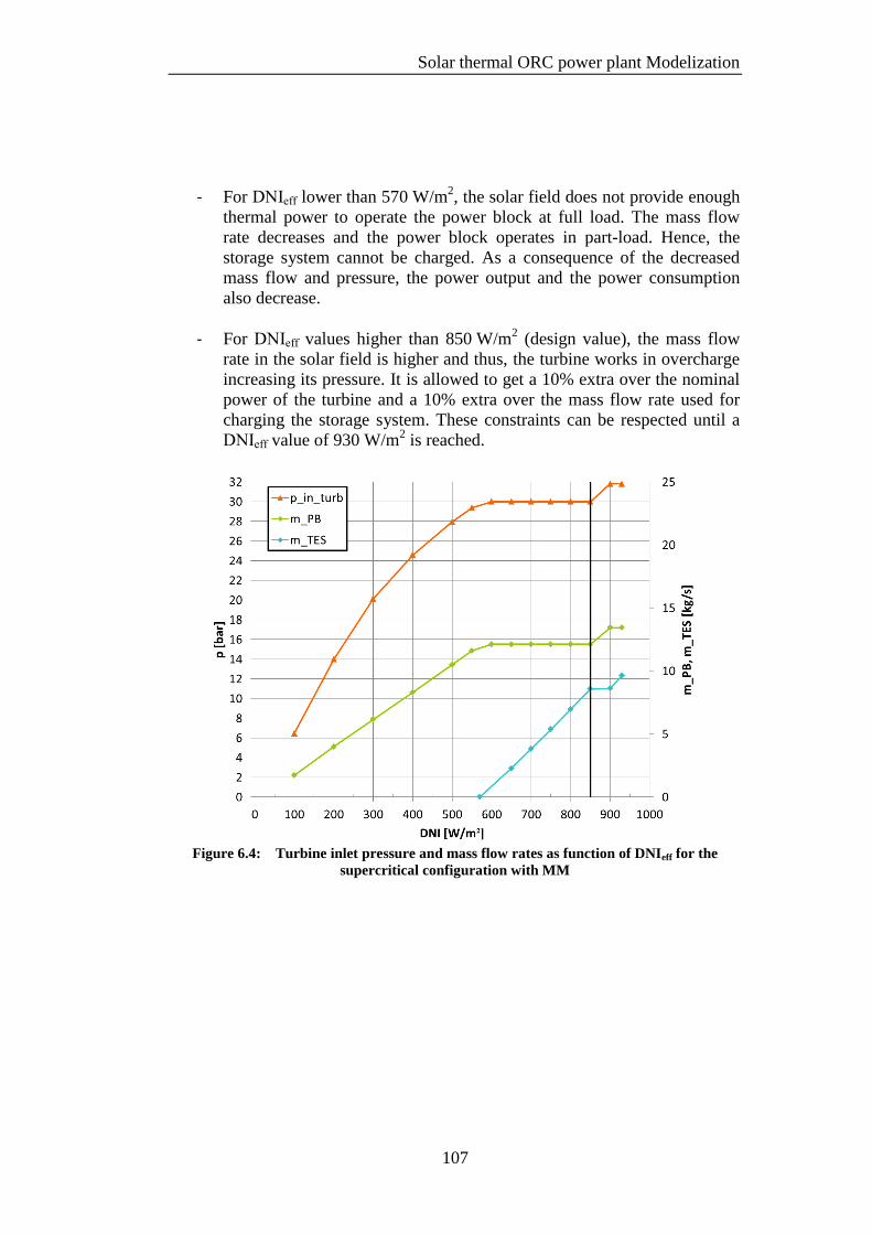
Solar thermal ORC power plant Modelization
107
- For DNIeff lower than 570 W/m2, the solar field does not provide enough
thermal power to operate the power block at full load. The mass flow
rate decreases and the power block operates in part-load. Hence, the
storage system cannot be charged. As a consequence of the decreased
mass flow and pressure, the power output and the power consumption
also decrease.
- For DNIeff values higher than 850 W/m2 (design value), the mass flow
rate in the solar field is higher and thus, the turbine works in overcharge
increasing its pressure. It is allowed to get a 10% extra over the nominal
power of the turbine and a 10% extra over the mass flow rate used for
charging the storage system. These constraints can be respected until a
DNIeff value of 930 W/m2 is reached.
Figure 6.4: Turbine inlet pressure and mass flow rates as function of DNIeff for the
supercritical configuration with MM
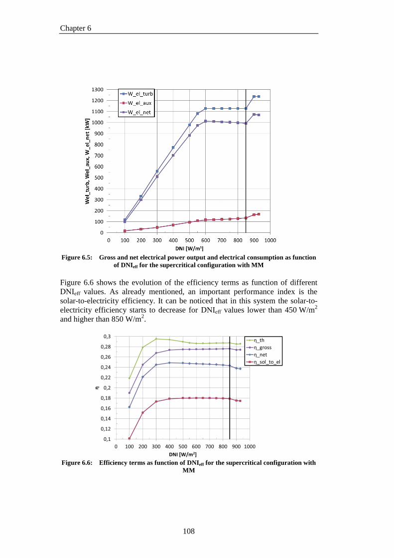
Chapter 6
108
Figure 6.5: Gross and net electrical power output and electrical consumption as function
of DNIeff for the supercritical configuration with MM
Figure 6.6 shows the evolution of the efficiency terms as function of different
DNIeff values. As already mentioned, an important performance index is the
solar-to-electricity efficiency. It can be noticed that in this system the solar-to-
electricity efficiency starts to decrease for DNIeff values lower than 450 W/m2
and higher than 850 W/m2.
Figure 6.6: Efficiency terms as function of DNIeff for the supercritical configuration with
MM

Solar thermal ORC power plant Modelization
109
Charging mode analysis
In order to ensure reliable operation of the heat exchanger in the charging mode,
a margin on the minimum mass flow rates that flow in the heat exchanger
should be set. The heat transfer characterstics are reported in a T-Q diagram, as
shown in Figure 6.7.
Figure 6.7: T-Q diagram of the charging process in the heat exchanger of the storage
system circuit in the supercritical configuration
According to the figure, it can be noted that the charging process can always be
performed since there is heat transfer rate in excess (wheter in design or in off-
design conditions).
Discharging and storage-only operation analysis
Referring to Figure 6.8, in case of the supercritical configuration, the molten salt
enters the heat exchanger at 275°C and leaves it at 190°C. For counter current
heat transfer, the cold organic fluid enters the exchanger at the regenerator outlet
temperature and exits at 270°C. In order to recover the maximum thermal power
of the TES system at these fixed temperatures, a mass flow rate of molten salt
equal to 30 kg/s is required. This value allows for a net power output equal to
96% of the design one. The heat transfer at these fixed temperatures can be
performed also in part-load until the pinch-point remains positive. The control
strategy allows for a decrease of the mass flow rate of the molten salt down to
approximately 80% of its design value. The outlet temperature of the molten salt
is maintained fixed, in order to avoid that the temperature of the cold tank

Chapter 6
110
increases. In fact, with an increased temperature of the cold tank, the storage
capacity will decrease.
Figure 6.8: T-Q diagram of the discharging process in the heat exchanger of the storage
system circuit in the supercritical configuration
Figure 6.9 shows in the T-s diagram the cycle layouts performed with the
storage-only operation. For a comparison the cycle layout performed with the
solar field at nominal conditions is also represented.
Figure 6.9: Comparison between the supercritical cycle layout perfomed with the solar
field at nominal conditions and the ones performed with the storage-only operation in a T-s
diagram

Solar thermal ORC power plant Modelization
111
Hence, the turbine inlet pressure, the mass flow rate of the organic fluid and the
power output can be parameterized as a function of the mass flow rate of the
molten salt, as reported in Figure 6.10.
Figure 6.10: Turbine inlet pressure, organic mass flow rate and power terms as function
of the mass flow rate of the molten salt for the storage-only operation
Furthermore, in order to evaluate the performances of the plant when the heat
source is represented by the TES system, , , and are calculated.
Figure 6.11 shows the defined performance indexes as function of the mass flow
rate of the molten salt.
Figure 6.11: Efficiency terms as function of the mass flow rate of the molten salt for the
storage-only operation mode

Chapter 6
112
6.2.2 Case-study: saturated cycle configuration
In case of the saturated configuration, the control strategy aims at providing
saturated vapor condition at the outlet of the solar field (Figure 6.12).
Figure 6.12: Subcritical saturated off-design cycle layouts
The sliding pressure control of the turbine can be maintained for each DNIeff
value and there is no need to use a throttle or a nozzle governing. The
evaluations in the change of the parameters and performances are quite similar
as the ones for the supercritical configuration (Figure 6.4 and Figure 6.5).
Nevertheless some differences can be drawn. As shown in Figure 6.13 and
Figure 6.14, the first difference is that in the saturated configuration the power
block can be run at full load until a DNIeff value of 600 W/m2, instead of
570 W/m2. Furthermore, for the saturated cycle configuration the evolution of
the recirculation mass flow rate is shown in Figure 6.13. Another important
difference is that for DNIeff values lower than 600 W/m2, all the efficiency terms
decrease more rapidly, as shown in Figure 6.15.

Solar thermal ORC power plant Modelization
113
Figure 6.13: Turbine inlet pressure and mass flow rates as function of DNIeff for the
saturated configuration with D4
Figure 6.14: Gross and net electrical power output and electrical consumption as function
of DNIeff for the saturated configuration with D4

Chapter 6
114
Figure 6.15: Efficiency terms as function of DNIeff for the saturated configuration with D4
Charging mode analysis
According to the Figure 6.16, it can be noted that the charging process in case of
the saturated configuration can always be performed and the conclusions drawn
for the supercritical case in the previous subsection are still valid.
Figure 6.16: T-Q diagram of the charging process in the heat exchanger of the storage
system circuit in the saturated configuration

Solar thermal ORC power plant Modelization
115
Discharging and storage-only operation analysis
Referring to the T-Q diagram for the saturated configuration (Figure 6.17), it
can be noted that the vaporizing stream is represented by a horizontal line.
Moreover, as a consequence of the constraint on the pinch-point ( = 5°C),
the organic fluid exits the heat exchanger at a temperature deeply lower than that
of the supercritical cycle.
In order to maintain a saturated layout, in this case only one specific mass flow
rate of the fluid ensures a proper thermal match with the heat source. In this case
the cycle performed is shown in a T-s diagram in Figure 6.18 and is
characterized by a turbine inlet temperature of 228.76°C. In such case, the
corresponding net power output would be very strongly decreased from the
nominal one (approximately 30% of the design capacity). A comparison of the
performance indexes between the cycle perfomed with the SF at nominal
conditions and the one performed with the storage-only operation is listed in
Table 6.2.
Figure 6.17: T-Q diagram of the discharging process in the heat exchanger of the storage
system circuit in the saturated configuration

Chapter 6
116
Figure 6.18: Comparison between the saturated cycle layout perfomed with the solar field
at nominal conditions and the one performed with the storage-only operation in a T-s
diagram
Table 6.2: Comparison between the performance indexes of the solar field at nominal
conditions and the one of the storage-only operation for a saturated configuration
Performance index SF design cycle Storage-only
operation cycle
981 kW 291 kW
941 kW 255 kW
809 kW 250 kW
23.9 % 20.5 %
22.9 % 18.0 %
19.7 % 17.6 %

Solar thermal ORC power plant Modelization
117
6.3 Simulation of typical days
In order to evaluate the feasibility of the control strategies mentioned in Section
5.8, a simulation of one day in three different seasons is carried out for both
plant configurations using the simulation results for design and off-design cases.
The data of the effective direct normal irradiation are taken from the EBSILON
database for a summer day (21st June 2009), a winter day (19
th December 2009)
and a mid-season day (25th
March 2009) in Lleida, Spain. Table 6.3 shows the
specification of the chosen site.
Table 6.3: Specification of the site
Site Lleida, Spain
longitude 0.56°E
latitude 41.58°N
Annual DNI 1758 kWh/m2
Average annual
temperature
14.6°C
6.3.1 Simulation of a summer day
Figure 6.19 presents the DNI, DNIeff and the IAM∙ ( ) data for the specific
daytime on 21st June 2009.
Figure 6.19: DNI, effective DNI and IAM∙cos(θi) on 21
st June 2009 in Lleida
Relevant system parameters for the both, supercritical and saturated
configurations are listed in Table 5.7. As described in Section 5.8 various
operating points can occure. As a simplification, a mode where the power block

Chapter 6
118
is operated by the solar field and by the storage system at the same time is not
considered. Thermal and electrical power for both systems are shown in Figure
6.20, while in Figure 6.21 the evolution of the charge-level of the TES is
presented. It must be noted that in case of the saturated configuration
(represented on the right), during storage-only operation the system is in low
part-load due to the constraints, that are explained in Section 6.2.2. This deep
part-load operation allows for electricity production until the early morning
hours (2 a. m.) but at a lower efficiency. In contrast to that, the supercritical
cycle works at almost full-load during storage-only operation. Therefore, the
plant operation already ends at 21:00.
Figure 6.20: Thermal and electrical power for the supercritical (left) and saturated (right)
configurations at a location of 41.58°N, 0.56°E for the meteorogical data of a summer day
(21st June 2009)
Figure 6.21: Net electric power output and thermal capacity for the supercritical (left) and
saturated (right) configuration at a location of 41.58°N, 0.56°E for the meteorogical data of
a summer day (21st June 2009)

Solar thermal ORC power plant Modelization
119
By observing the results, the following conclusions can be drawn:
- The daily thermal power from the solar field and net electricity output is
higher in the supercritical configuration than in the saturated one.
- The daily solar-to-electricity efficiency is also higher in the supercritical
case than in the saturated one: 17.1% compared to 14.1%.
- In the supercritical cycle, the power block works almost at nominal load,
entailing a high efficiency. Due to that, systems with large storage
capacities could be realized offering the possibility of base-load
operation.
- In the saturated cycle, the power block works at low part-load during
storage-only operation. This operating mode leads to a lower efficiency
and, furthermore, systems with large storage capacities cannot be
realized since there would not be enough time for the discharge
operation during the night.
Table 6.4 summarizes the obtained results for a typical summer day.
Table 6.4: Results of the daily calculation for a typical summer day (21st June 2009)
Description Supercritical
configuration
Saturated
configuration
Daily DNI·net aperture area 85 724 kWh
Daily DNIeff·net aperture area 84 098 kWh
Daily thermal power from solar field 60 810 kWh 60 675 kWh
Daily net electricity output 14 697 kWh 12 126 kWh
Average solar field thermal efficiency 70.9% 70.8%
Average solar-to-electricity efficiency 17.1% 14.1%
6.3.2 Simulation of a winter day
Figure 6.19 presents the DNI, DNIeff and the IAM∙ ( ) data for the specific
daytime on 19th
December 2009.

Chapter 6
120
Figure 6.22: DNI, effective DNI and IAM∙cos(θi) on 19
th December 2009 in Lleida
Thermal and electrical power for both systems are shown in Figure 6.20. It must
be noted that the thermal power input in such day is not high enough to run the
systems at full-load. Both systems are run in part-load from 8 a. m. till 4 p. m.
and the storage system remains completely empty.
Figure 6.23: Thermal and electrical power for the supercritical (left) and saturated (right)
configurations at a location of 41.58°N, 0.56°E for the meteorogical data of a winter day
(19th
December 2009)

Solar thermal ORC power plant Modelization
121
Table 6.5 summarizes the obtained results for a typical winter day. As a
consequence of the low DNIeff values, the electricity outputs and the efficiency
terms are highly decreased.
Table 6.5: Results of the daily calculation for a typical winter day (19th
December 2009)
Description Supercritical
configuration
Saturated
configuration
Daily DNI·net aperture area 52 172 kWh
Daily DNIeff·net aperture area 25 318 kWh
Daily thermal power from solar field 17 926 kWh 17 942 kWh
Daily net electricity output 4 347 kWh 3 469 kWh
Average solar field thermal efficiency 34.4% 34.4%
Average solar-to-electricity efficiency 8.3% 6.6%
6.3.3 Simulation of a mid-season day
Figure 6.24 presents the DNI, DNIeff and the IAM∙ ( ) data for the specific
daytime on 25th
March 2009.
Figure 6.24: DNI, effective DNI and IAM∙cos(θi) on 25
th March 2009 in Lleida
Thermal and electrical power for both systems are shown in Figure 6.25, while
in Figure 6.26 the evolution of the charge-level of the TES is presented. It must
be noticed that similar conclusion of Section 6.3.1 can be drawn. The main
difference is that in such day the DNIeff is lower compared to that in a summer
day. The charge-level of the TES system reaches approximately 30% of its total
capacity.

Chapter 6
122
Figure 6.25: Thermal and electrical power for the supercritical (left) and saturated (right)
configurations at a location of 41.58°N, 0.56°E for the meteorogical data of a mid-season
day (25th
March 2009)
Figure 6.26: Net electric power output and thermal capacity for the supercritical (left) and
saturated (right) configuration at a location of 41.58°N, 0.56°E for the meteorogical data of
a mid-season day (25th
March 2009)
Table 6.6 summarizes the obtained results for a typical mid-season day.

Solar thermal ORC power plant Modelization
123
Table 6.6: Results of the daily calculation for a typical mid-season day (25th
March
2009)
Description Supercritical
configuration
Saturated
configuration
Daily DNI·net aperture area 78 288 kWh
Daily DNIeff·net aperture area 66 954 kWh
Daily thermal power from solar field 48 778 kWh 48 610 kWh
Daily net electricity output 11 736 kWh 10 207 kWh
Average solar field thermal efficiency 62.3% 62.1%
Average solar-to-electricity efficiency 15.0% 13.0%

124

125
Conclusions
In the present thesis ORC processes for direct steam generation in parabolic
trough power plants have been investigated and evaluated. Focus has been set on
providing new solutions for power cycles that combine the direct steam
generation of an organic medium in a parabolic trough plant.
In Chapter 1 state-of-the art CSP plants are discussed, focusing on the different
types of parabolic trough systems including integrated storage system.
New technologies are currently being developed that shall increase the
efficiency and reduce the cost of next-generation trough plants. While in the
sector of large-scale plants Direct Steam Generation and Molten Salt systems
are developed, ORC systems could offer a promising option for small-scale off-
grid and co-generation applications.
In Chapter 2 a technical background about ORC has been given. An ORC offers
simple cycle design and specific properties, which reduce the complexity of the
turbine design. These advantages make organic Rankine cycles particularly
attractive for small-scale parabolic trough solar applications. There is a variety
of ORC fluids with different thermodynamic characteristics available being
suited for different working temperature ranges. Therefore, Chapter 3 is focused
on the choice of the organic working fluid. The research has been concentrated
on finding the most suitable fluids for a solar DSG application in accordance
with the multitude of constraints related to the thermodynamic properties of the
fluids, as well as considerations of health, safety and environmental impact. In
particular, the organic fluid that circulates through the solar field must be
environmental-friendly and meet basic requirements such as safety and technical
suitability. Only few fluids meet the selection criteria of Section 3.1. Therefore,
a trade-off has been made and a set of possible working fluid candidates have
been identified using heuristic knowledge about the processes based on similar
systems. The investigated fluids have been selected in order to deal with
different maximum temperature values between 200°C and 400°C, typical
values reached from existing parabolic trough systems. When low-temperature
applications (< 250°C) are considered, fluids like R245fa and SES36, currently
employed in geothermal applications and characterized by a low critical
temperature, can be used. For high-temperature applications (> 250°C), fluids
with the highest possible critical temperature should be selected in order to
allow operating a subcritical ORC with limited pressure. Among the
investigated fluids with a high critical temperature, cyclic and linear siloxanes
have been selected as the most promising also due to their environmental
friendly characteristics and their maximum achievable temperatures (300°C for
linear siloxanes and 340°C for cyclic siloxanes [75]).

Conclusions
126
In order to take advantage of the achievable temperatures of the PTCs and in
accordance with the research fields of the Line Focus Systems division of DLR,
the main interest has been set on high temperature processes. Therefore, in
Chapter 4 the basic single-pressure cycle layouts with siloxanes have been
analysed, focusing in detail on a saturated process with the fluid D4 and a
supercritical process with MM. It must be mentioned that the process with D4
can guarantee the respect of the specific optimization criteria, defined in Section
4.3, only with relatively high condensing temperature (87.3°C). For that reason
this fluid should be normally taken with high condensing temperatures for
combined heat and power systems (CHP). On the other hand, the supercritical
cycle with MM allows operating with actual air-cooled condensers (condensing
temperature of 45°C), achieving high performances in terms of specific net
work. Analysis has also concluded that for a supercritical cycle with a fixed
turbine inlet temperature, the cycle efficiency has its maximum value with a
inlet pressure close to the critical pressure value and decreases as the pressure
increases. Subsequently, the integration of TES system in the solar ORC
processes has been discussed. Most of the investigated TES systems are still
proof-concepts for DSG applications, as e.g. the PCM storage system. Among
all the possible combinations, only the one with the indirect two-tank storage
system has been indicated to be technically feasible for both a saturated and a
supercritical process. Nevertheless, for those two case-studies the thermal match
between the heat source and the fluid has shown to be rather different. It might
be outlined that, compared to the supercritical configuration, in the saturated one
the need to store as well sensible as latent heat leads to a higher decrease of the
steam parameters between charging and discharging processes. In order to
evaluate the performances of a solar thermal DSG power plant based on those
two chosen configurations and coupled with an indirect two-tank storage
system, computer modeling and simulations have been carried out using the
software EBSILON®Professional 10.05 in Chapter 5. Both plant configurations
have been properly sized with the same solar field (6 collector loops of the
model Eurotrough ET150) and TES system (4 hours at full load capacity).
EBSILON is a very stable tool for power plant simulations with traditional
water steam cycles. However, the combination of components of the solar
library in combination with direct steam generation of an organic fluid led to
convergence problems. In order to make design and off-design simulations
successfully converge, a trade-off in the layout of both models has been made.
Some pipes have been physically decoupled and boundary conditions have been
set using transmitter elements. Chapter 6 has been devoted to the evaluation of
the simulation results. First simulation has been performed at nominal
conditions, which showed that the supercritical configuration could reach higher
efficiencies ( =17.8%) and power outputs ( =992 kWel) compared
to the the saturated one (respectively, =14.6%; =809 kWel). This

Conclusions
127
is mostly due to the adopted constraint on the condensing pressure of the cycles.
In a second step, the behavior in part-load operation during lower irradiation
conditions has been evaluated. The net power generation has achieved the
maximum and minimum value for the highest and lowest values of the mass
flow rates in the PB, respectively. As expected, the results have shown that the
efficiency decreases as both mass flow rates and pressure decrease. In
conclusion, specific interest has been dedicated to assess the integration of the
indirect two-tank storage system in charging and discharging modes. Off-design
results have shown that charging well occurs since there is enough thermal
power available to run the power block at full load ( 4083 kWth and
4104 kWth for supercritical and saturated configuration, respectively).
On the other hand, discharging and storage-only operations occur with some
thermodynamic limitations imposed by the pinch-point in the heat exchanger.
The case-study of the supercritical configuration has shown that discharging at
fixed temperatures could be performed until the pinch-point remains positive. A
net power output equal to 96% of the design one has been reached when the
mass flow rate of molten salt has been set equal to 30 kg/s. In the saturated case,
only one specific combination of molten salt and ORC mass flow rate has been
found feasible during the discharge mode, due to pinch point limitations. The
corresponding net power output has been found to be 30% of the design
capacity. It must be concluded that the integration of an indirect two-tank
storage system is a feasible but not optimal solution. As demonstrated in the
simulation for a typical summer day, only the supercritical configuration offers
the possibility to integrate large storage systems for base-load operation. In
future studies the integration of storage systems shall be further optimized.
Research shall be centered on technological issues, such as material
requirements and detailed process component design. Furthermore, a techno-
economical analysis about materials and equipments used are required in order
to prove the feasibility of the systems as a whole. This study led to the
conclusion that direct steam generation of an organic fluid in parabolic trough
solar plants with an integrated indirect two-tank storage system is theoretically
feasible. In order to assess the dynamic behaviour of the whole plants, the
implementation of a detailed control strategy is required and could constitute a
future research study. In addition, an annual simulation to assess the electric
energy production together with an economic analysis to estimate the levelized
cost of the electricity produced by the systems should be carried out.

128

I
Appendix
Optical and geometrical losses in a PTC
The following section gives a further describtion of the optical and geometrical
losses that must be taken into account to calculate the heat that is absorbed by
the receiver. As mentioned in Chapter 5, Section 5.3.2, the incoming optical
thermal power of the collector in W/m2 is given by
( ) ( ) (A.1)
with:
- : direct normal irradiation;
- : optical peak efficiency;
- : reflecting mirror cleanliness factor;
- : shading loss factor;
- : end loss factor;
- ( ) : incident angle modifier as a function of in degree;
- : focusing state of the collector.
Optical peak efficiency
The incoming solar radiation on the collector aperture is never fully converted
into usable heat. As shown in Figure A.1, optical losses occur and are associated
with four parameters that are:
1. The mirror reflectivity, : This parameter represents the ratio between
the portion of the reflected radiation and the unitary incident radiation.
The typical value for this parameter in PTCs is 0.9. Being less than 1, it
means that only part of the incident radiation is reflected by the absorber
tube and losses occur.
2. The intercept factor, : This index quantifies the losses due to either
microscopic imperfections of the reflectors or macroscopic shape errors
in the parabolic trough concentrators. Thus, a part of the incident sun
rays reflected by the mirrors is deviated from the optimal direction and
does not intercept the absorber tube. Its typical value for PTCs is around
0.95.
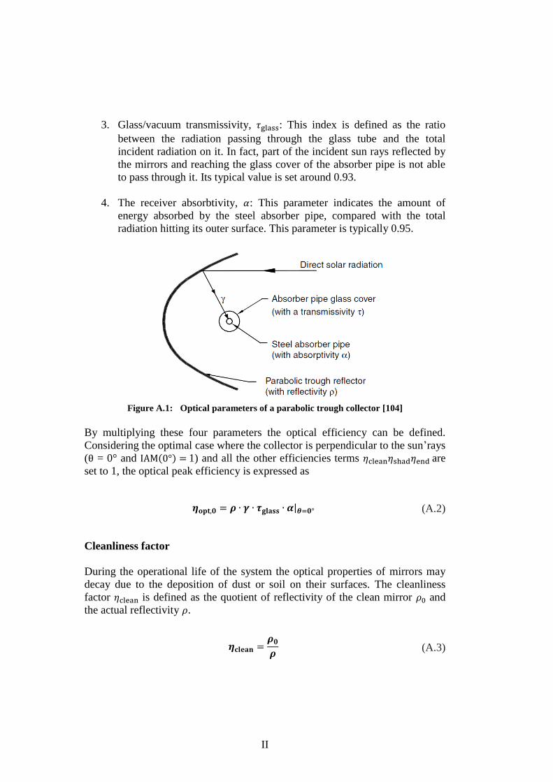
II
3. Glass/vacuum transmissivity, : This index is defined as the ratio
between the radiation passing through the glass tube and the total
incident radiation on it. In fact, part of the incident sun rays reflected by
the mirrors and reaching the glass cover of the absorber pipe is not able
to pass through it. Its typical value is set around 0.93.
4. The receiver absorbtivity, : This parameter indicates the amount of
energy absorbed by the steel absorber pipe, compared with the total
radiation hitting its outer surface. This parameter is typically 0.95.
Figure A.1: Optical parameters of a parabolic trough collector [104]
By multiplying these four parameters the optical efficiency can be defined.
Considering the optimal case where the collector is perpendicular to the sun’rays
( = 0° and ( ) 1) and all the other efficiencies terms are
set to 1, the optical peak efficiency is expressed as
| (A.2)
Cleanliness factor
During the operational life of the system the optical properties of mirrors may
decay due to the deposition of dust or soil on their surfaces. The cleanliness
factor is defined as the quotient of reflectivity of the clean mirror and
the actual reflectivity .
(A.3)

III
Shading loss factor
The shading phenomenon occurs generally during the morning and in the
evening. As shown in Figure A.2, a part of the collector’s aperture gets shaded
from the next one, thus preventing the direct beam to reach the collector.
Figure A.2: Shaded collectors [91]
In order to express the losses due to shading, the efficiency factor is used.
It can be defined as
(
) (A.4)
where is the number of collector rows in parallel which have the potential
to shade each other, is the collector’s aperture width, the distance
between the collector rows and the collector tracking angle.
Endloss factor
End losses occur when the incident angle (the angle between the normal to
the aperture plane of the collector and the sun’s vector, both contained on a
plane perpendicular to the collector axis) is higher than 0°. Thus, as shown in
Figure A.3, the solar radiation does not hit the mirrored surface perpendicularly.
As the mirror field and the receiver tube are not infinite, parts of the tube are
sometimes inactive, while a part of the light is reflected outside the tube. In the
case of several collectors in a row, if the reflected solar radiation hits the
receiver of the neighbouring collector, end losses can be partly compensated.

IV
The endloss efficiency is defined as
(A.5)
with:
: focal length (vertical distance between receiver axis and mirror surface)
: collector length
: incidence angle of direct solar radiation
: end gains that occur when there are more than one collector in a row
The factor can be calculated with the number of collectors in one row
and their distance , as expressed in Equation (A.6).
( )
(A.6)
Figure A.3: End effects [91]

V
References
[1] International Energy Agency IEA. 2012; Available from:
http://www.iea.org/.
[2] Kalogirou, S.A., Solar energy engineering: processes and systems2009:
Academic Press.
[3] IEA, Solar Energy Perspectives. 2011.
[4] Al-Sulaiman, F.A., Energy and sizing analyses of parabolic trough solar
collector integrated with steam and binary vapor cycles. Energy, 2013.
58: p. 561-570.
[5] Turboden. Available from: www.turboden.eu.
[6] Šúri, M., et al., Comparison of direct normal irradiation maps for
Europe. Proceeding of the SolarPACES, 2009.
[7] Price, H., et al., Advances in parabolic trough solar power technology.
Journal of solar energy engineering, 2002. 124(2): p. 109-125.
[8] Fernández-García, A., et al., Parabolic-trough solar collectors and their
applications. Renewable and Sustainable Energy Reviews, 2010. 14(7):
p. 1695-1721.
[9] Giostri, A., et al. Comparison of Two Linear Collectors in Solar Thermal
Plants: Parabolic Trough vs Fresnel. in Proceedings of the ASME 2011
International Conference on Energy Sustainability. 2011.
[10] Abbas, R., et al., Solar radiation concentration features in Linear
Fresnel Reflector arrays. Energy Conversion and Management, 2012.
54(1): p. 133-144.
[11] NREL. NREL: Concentrating Solar Power Projects - Ivanpah Solar
Electric Generating System. 2013; Available from:
http://www.nrel.gov/csp/solarpaces/project_detail.cfm/projectID=62.
[12] J., T.-K.K. and B. M, Erneuerbare Energien, Band 22009: Neuruppin.
[13] Kalogirou, S.A., Solar thermal collectors and applications. Progress in
energy and combustion science, 2004. 30(3): p. 231-295.
[14] Laboratories, S.N. Sandia, Stirling Energy Systems set new world record
for solar-to-grid conversion efficiency. 07.02.2014]; Available from:
https://share.sandia.gov/news/resources/releases/2008/solargrid.html.
[15] SolarPaces. Technology Characterization Solar Dish Systems.
07.02.2014]; Available from:
http://www.solarpaces.org/CSP_Technology/docs/solar_dish.pdf.
[16] Solutia Therminol VP-1 Product Data Sheet.
[17] Group, E.W., Solar thermal energy production: guidelines and future
programmes of ENEA. ENEA Report, 2001, ENEA/TM/PRESS/2001-07.

VI
[18] Kearney, D., et al., Assessment of a molten salt heat transfer fluid in a
parabolic trough solar field. Journal of solar energy engineering, 2003.
125(2): p. 170-176.
[19] ENEA. Archimede Project. 07.02.2014]; Available from:
http://www.archimedesolarenergy.it/enea_archimede_project.htm.
[20] Zarza, E., et al., Direct steam generation in parabolic troughs: Final
results and conclusions of the DISS project. Energy, 2004. 29(5-6): p.
635-644.
[21] Zarza, E., et al., The DISS Project: Direct Steam Generation in
Parabolic Trough Systems. Operation and Maintenance Experience and
Update on Project Status. Journal of Solar Energy Engineering, 2002.
124(2): p. 126.
[22] Zarza, E., et al., INDITEP: The first pre-commercial DSG solar power
plant. Solar Energy, 2006. 80(10): p. 1270-1276.
[23] Zarza, E., et al., DISS-phase I project. Final project report, Editorial
CIEMAT, Madrid, Spain, 1999.
[24] Hellwig, U., J. Peterseim, and P. Widera, Water Circulation Calculation
for Concentrated Solar Thermal Plants.
[25] Chemieingenieurwesen, V.-G.V.u. and V. Gesellschaft, VDI Heat
Atlas2010: Springer.
[26] Eck, M., et al., Field test of water-steam separators for direct steam
generation in parabolic troughs. Journal of solar energy engineering,
2008. 130(1): p. 011002.
[27] Feldhoff, J.F., et al., Status and first results of the DUKE project -
Component qualification of new receivers and collectors, in 19th
SolarPACES Conference2013: Las Vegas, NV, USA.
[28] Steinmann, W.-D. and R. Tamme, Latent Heat Storage for Solar Steam
Systems. Journal of Solar Energy Engineering, 2008. 130(1): p. 011004.
[29] Laing, D., et al., Thermal energy storage for direct steam generation.
Solar Energy, 2011. 85(4): p. 627-633.
[30] Steinmann, W.-D. and M. Eck, Buffer storage for direct steam
generation. Solar Energy, 2006. 80(10): p. 1277-1282.
[31] Feldhoff, J.F., et al., Comparative system analysis of direct steam
generation and synthetic oil parabolic trough power plants with
integrated thermal storage. Solar Energy, 2012. 86(1): p. 520-530.
[32] Canada, S., et al., Parabolic Trough Organic Rankine Cycle Solar Power
Plant. 2004 DOE Solar Energy Technologies, 2005.
[33] Canada, S.B., D, et al., Status of APS 1-MWe Parabolic Trough Project.
2005 DOE Solar Energy Technologies, 2005.
[34] Holaniku at Keahole Point Micro CSP Thermal Plant, United States of
America. 07.01.2014]; Available from: http://www.power-
technology.com/projects/holanikuatkeaholepoi/.

VII
[35] Quoilin, S., An introduction to thermodynamics applied to Organic
Rankine Cycles. 2008.
[36] Quoilin, S., et al., Techno-economic survey of Organic Rankine Cycle
(ORC) systems. Renewable and Sustainable Energy Reviews, 2013. 22:
p. 168-186.
[37] Tchanche, B.F., et al., Low-grade heat conversion into power using
organic Rankine cycles – A review of various applications. Renewable
and Sustainable Energy Reviews, 2011. 15(8): p. 3963-3979.
[38] Chen, H., D.Y. Goswami, and E.K. Stefanakos, A review of
thermodynamic cycles and working fluids for the conversion of low-
grade heat. Renewable and Sustainable Energy Reviews, 2010. 14(9): p.
3059-3067.
[39] Wang, J., J. Zhang, and Z. Chen, Molecular Entropy, Thermal
Efficiency, and Designing of Working Fluids for Organic Rankine
Cycles. International Journal of Thermophysics, 2012. 33(6): p. 970-985.
[40] Angelino, G. and P. Colonna di Paliano, Multicomponent Working
Fluids For Organic Rankine Cycles (ORCs). Energy, 1998. 23(6): p.
449-463.
[41] Wang, X.D. and L. Zhao, Analysis of zeotropic mixtures used in low-
temperature solar Rankine cycles for power generation. Solar Energy,
2009. 83(5): p. 605-613.
[42] Schuster, A., S. Karellas, and R. Aumann, Efficiency optimization
potential in supercritical Organic Rankine Cycles. Energy, 2010. 35(2):
p. 1033-1039.
[43] Group of Energy Conversion Systems (Gecos), State of the art of ORC.
Technical Report, Politecnico di Milano, 2013.
[44] Gaia, M. “30 Years of Organic Rankine Cycle Development. in First
International Seminar on ORC Power Systems, Keynote Lecture. 2011.
[45] Angelino, G., M. Gaia, and E. Macchi, A review of Italian activity in the
field of organic Rankine cycles. VDI-Berichte, 1984(539): p. 465-482.
[46] Baskharone, E.A., Principles of turbomachinery in air-breathing
engines2006: Cambridge University Press.
[47] Obernberger, I., P. Thonhofer, and E. Reisenhofer, Description and
evaluation of the new 1,000 kWel Organic Rankine Cycle process
integrated in the biomass CHP plant in Lienz, Austria. Euroheat &
Power, 2002. 10(1): p. 18-25.
[48] Lund, J.W., Combined Heat and Power Plant–Neustadt-Glewe,
Germany. Geo-Heat Center Quarterly Bulletin, 2005. 26(2): p. 31-34.
[49] Canada, S., et al., Parabolic Trough Organic Rankine Cycle Solar Power
Plant. 2004 DOE Solar Energy Technologies, 2005.
VIII
[50] Quoilin, S., et al., Performance and design optimization of a low-cost
solar organic Rankine cycle for remote power generation. Solar Energy,
2011. 85(5): p. 955-966.
[51] Lai, N.A., M. Wendland, and J. Fischer, Working fluids for high-
temperature organic Rankine cycles. Energy, 2011. 36(1): p. 199-211.
[52] Saleh, B., et al., Working fluids for low-temperature organic Rankine
cycles. Energy, 2007. 32(7): p. 1210-1221.
[53] Shengjun, Z., W. Huaixin, and G. Tao, Performance comparison and
parametric optimization of subcritical Organic Rankine Cycle (ORC)
and transcritical power cycle system for low-temperature geothermal
power generation. Applied Energy, 2011. 88(8): p. 2740-2754.
[54] Ozone-Depletion and Chlorine-Loading Potential of
Chlorofluorocarbon Alternatives. Available from:
http://www.ciesin.org/TG/OZ/odp.html.
[55] GWP - Definition. Available from: http://en.wikipedia.org/wiki/Global-
warming_potential.
[56] IPCC. Available from: http://www.ipcc.ch/.
[57] ASHRAE, A., Standard 34-2001, Designation and safety classification
of refrigerants. American society of heating, refrigerating, and air-
conditioning engineers, Atlanta, GA, 2001.
[58] Drescher, U. and D. Brüggemann, Fluid selection for the Organic
Rankine Cycle (ORC) in biomass power and heat plants. Applied
Thermal Engineering, 2007. 27(1): p. 223-228.
[59] Borsukiewicz-Gozdur, A. and W. Nowak, Comparative analysis of
natural and synthetic refrigerants in application to low temperature
Clausius–Rankine cycle. Energy, 2007. 32(4): p. 344-352.
[60] Zhang, F.-Z. and P.-X. Jiang, Thermodynamic analysis of a binary
power cycle for different EGS geofluid temperatures. Applied Thermal
Engineering, 2012. 48(0): p. 476-485.
[61] Walraven, D., B. Laenen, and W. D’haeseleer, Comparison of
thermodynamic cycles for power production from low-temperature
geothermal heat sources. Energy Conversion and Management, 2013.
66(0): p. 220-233.
[62] Badr, O., P. O'Callaghan, and S. Probert, Rankine-cycle systems for
harnessing power from low-grade energy sources. Applied Energy,
1990. 36(4): p. 263-292.
[63] Invernizzi, C., P. Iora, and P. Silva, Bottoming micro-Rankine cycles for
micro-gas turbines. Applied Thermal Engineering, 2007. 27(1): p. 100-
110.
[64] Lemort, V., et al., Contribution à l'étude des cycles de Rankine de
récupération de chaleur, VIIIème Colloque Interuniversitaire Franco-
IX
Québécois sur la Thermique des Systèmes, Montréal, Canada, 2007,
ART-05-03.
[65] Liu, B.-T., K.-H. Chien, and C.-C. Wang, Effect of working fluids on
organic Rankine cycle for waste heat recovery. Energy, 2004. 29(8): p.
1207-1217.
[66] Dai, Y., J. Wang, and L. Gao, Parametric optimization and comparative
study of organic Rankine cycle (ORC) for low grade waste heat
recovery. Energy Conversion and Management, 2009. 50(3): p. 576-582.
[67] Lakew, A.A. and O. Bolland, Working fluids for low-temperature heat
source. Applied Thermal Engineering, 2010. 30(10): p. 1262-1268.
[68] Quoilin, S., et al., Thermo-economic optimization of waste heat recovery
Organic Rankine Cycles. Applied Thermal Engineering, 2011. 31(14): p.
2885-2893.
[69] Tchanche, B.F., et al., Fluid selection for a low-temperature solar
organic Rankine cycle. Applied Thermal Engineering, 2009. 29(11–12):
p. 2468-2476.
[70] Facão, J., A. Palmero-Marrero, and A.C. Oliveira, Analysis of a solar
assisted micro-cogeneration ORC system. International Journal of Low-
Carbon Technologies, 2008. 3(4): p. 254-264.
[71] Angelino, G. and C. Invernizzi, Experimental investigation on the
thermal stability of some new zero ODP refrigerants. International
journal of refrigeration, 2003. 26(1): p. 51-58.
[72] EPA raises GWP Tariff on R245fa. Available from:
http://www.infinityturbine.com/ORC/News/Entries/2012/5/2_Price_spik
es_in_USA_for_R245fa.html.
[73] Fröba, A. and e. al, Thermophysikalische Eigenschaften eines
Kältemittelgemisches aus R365mfc (1,1,1,3,3-Pentafluorbutan) und
Galden ® HT 55(Perfluorpolyether). DKV Conference 2005, 2005.
[74] Bombarda, P. and M. Gaia. Geothermal binary plants utilising an
innovative non-flammable, azeotropic mixture as working fluid. in
Proceedings 28th NZ Geothermal Workshop. 2006.
[75] Fernández, F.J., M.M. Prieto, and I. Suárez, Thermodynamic analysis of
high-temperature regenerative organic Rankine cycles using siloxanes
as working fluids. Energy, 2011. 36(8): p. 5239-5249.
[76] Colonna, P., A. Guardone, and N.R. Nannan, Siloxanes: A new class of
candidate Bethe-Zel’dovich-Thompson fluids. Physics of Fluids, 2007.
19(8): p. 086102.
[77] Dow Syltherm 800 Product Data Sheet.
[78] Angelino, G. and C. Invernizzi, Cyclic methylsiloxanes as working fluids
for space power cycles. Journal of Solar Energy Engineering;(United
States), 1993. 115(3).
[79] CoolProp. Available from: http://coolprop.sourceforge.net/.

X
[80] Mago, P.J., et al., An examination of regenerative organic Rankine
cycles using dry fluids. Applied Thermal Engineering, 2008. 28(8–9): p.
998-1007.
[81] Astolfi, M., et al., Binary ORC (organic Rankine cycles) power plants
for the exploitation of medium–low temperature geothermal sources –
Part A: Thermodynamic optimization. Energy, (0).
[82] Astolfi, M., et al., Binary ORC (Organic Rankine Cycles) power plants
for the exploitation of medium–low temperature geothermal sources–
Part B: Techno-economic optimization. Energy, 2014.
[83] Colonna, P. and J. Larjola, Siloxanes as Working Fluids for Mini-ORC
Systems Based on High-Speed Turbogenerator Technology. Journal of
Engineering for Gas Turbines and Power, 2013. 135: p. 042305-1.
[84] Angelino, G., C. Invernizzi, and E. Macchi, Organic working fluid
optimization for space power cycles, in Modern Research Topics in
Aerospace Propulsion1991, Springer. p. 297-326.
[85] Stenglein, M., et al., Novel Approach of Thermal Energy Storage
Systems in Concentrated Solar Power Plants with Direct Steam
Generation.
[86] Tamme, R., et al., Latent heat storage above 120 C for applications in
the industrial process heat sector and solar power generation.
International Journal of energy research, 2008. 32(3): p. 264-271.
[87] DLR, Personal Communication.
[88] NIST. Available from: http://www.nist.gov/srd/nist23.cfm.
[89] Pawellek, R., T. Löw, and T. Hirsch. EbsSolar—A Solar Library for
EBSILON® Professional. in Proceedings of the SolarPACES 2009
Conference. 2009.
[90] German Institute for Standardization, DIN 5034, part 2, Beuth Verlag.
[91] Schenk, H. and M. Eck, Yield analysis for parabolic trough solar
thermal power plants - a basic approach. DLR Report, 2012.
[92] Benz, N., Parabolrinnenkollektoren: Feldtest, Optimierung und
Weiterentwicklung von Receivern (PARFOR). 2008.
[93] Forristall, R.E., Heat transfer analysis and modeling of a parabolic
trough solar receiver implemented in engineering equation solver2003:
National Renewable Energy Laboratory.
[94] Burkholder, F. and C.F. Kutscher, Heat loss testing of schott's 2008
PTR70 parabolic trough receiver2009: National Renewable Energy
Laboratory.
[95] Friedel, L. Improved friction pressure drop correlations for horizontal
and vertical two-phase pipe flow. in European two-phase flow group
meeting, Paper E. 1979.
[96] Kelly, B. and D. Kearney, Parabolic trough solar system piping model.
Final Report, National Renewable Energy laboratory, 2006.

XI
[97] Price, H. A parabolic trough solar power plant simulation model. in
ASME 2003 International Solar Energy Conference. 2003. American
Society of Mechanical Engineers.
[98] Bonacina, L., Ottimizzazione energetica e analisi economica di impianti
geotermici binari in applicazione cogenerativa, 2011, Politecnico di
Milano: Milano.
[99] Stodola, A., Dampf-und Gasturbinen: mit einem Anhang über die
Aussichten der Wärmekraftmaschinen. Vol. 1. 1922: J. Springer.
[100] Menny, K., Strömungsmaschinen, in Hydraulische und thermische Kraft-
und Arbeitsmaschinen2006, Teubner: Wiesbaden. p. Online-Ressource
(X, 327S. 227 Abb, digital).
[101] Macchi, E. and A. Perdichizzi. Theoretical prediction of the off-design
performance of axial-flow turbines. in Proceedings Atti del XXXII
Congresso Nazionale ATI, Roma. 1977.
[102] Astolfi, M., et al., Technical and economical analysis of a solar–
geothermal hybrid plant based on an Organic Rankine Cycle.
Geothermics, 2011. 40(1): p. 58-68.
[103] Singh, O., Applied Thermodynamics. 3rd ed2009: New Age
International.
[104] Goswami, D.Y. and F. Kreith, Handbook of energy efficiency and
renewable energy2007: Crc Press.