Evaluation of Non-Nuclear Gauges to Measure Density of Hot-Mix Asphalt Pavements

Pooled Fund Study

Final Report

Prepared by

Pedro Romero, Ph.D., P.E. The University of Utah

Department of Civil and Environmental Engineering

July 18, 2002

i

Executive Summary

A study was conducted to evaluate if the commercially available non-nuclear density gauges could be used to determine density of hot-mix asphalt (HMA) pavements. Comparisons were made, both in the laboratory and in the field, between accepted density values of HMA and density obtained from both the Pavement Quality Indicator (PQI) and the PaveTracker.

A laboratory study conducted in 1999 indicated that the PQI model 300

had a linear output relation between the changes in density of HMA slabs when measured under constant temperature and humidity conditions for a single asphalt mixture. The study indicated that, to measure density in the field, a calibration procedure that is mixture specific should be carried out. The study also indicated that it is necessary to correct for changes in moisture and temperature.

Based on the results from the laboratory study, a field study was

conducted during the 2000 construction season. The results of the field study indicated that the sensitivity of the PQI-300 was not adequate to measure density changes in the field. The study recommended changes in both the sensitivity of the device and the algorithms used to correct for moisture and temperature.

After several improvements were made to the PQI device and the

introduction of the PaveTracker, a second field study was conducted during the 2001 construction season. The results showed an improvement over the previous study. Based on the results of the 2001 field study it was concluded that, in order to use non-nuclear gauges to obtain absolute pavement density, calibration using the same materials is needed. Since this is often difficult to accomplish without the construction of test sections, neither the modified PQI-300 nor the PaveTracker were considered suitable to measure pavement density for quality acceptance (QA) purposes or to determine pay factors. However, the devices were accurate for quality control (QC) applications. Based on the results from this research, the eased in which these devices can be operated, and their ability to provide immediate feedback of density changes; both non-nuclear density gauges evaluated are considered ideal to locate spots with or sections with low density thus trigger corrective actions leading to more uniform pavements.

ii

Acknowledgements

The support from the state highway agencies of Maryland, Pennsylvania, New York, Minnesota, Connecticut, and Oregon, as well as the Federal Highway Administration’s Turner-Fairbank Highway Research Center is greatly appreciated. Special mention goes to Gloria Burke from Maryland State Highway Administration, Thomas Harman from FHWA TFHRC, and Ewa Rodzig from FHWA who handle most of the administrative issues. Jared Morse, Bernie Fitzgerald, and John Hewitt from TransTech Systems Inc. as well as Don Geisel from Donald J. Geisel and Associates Inc. provided technical support in the use of their respective product. Their work is acknowledged.

This work resulted in a masters thesis at The University of Utah by

Frederick Kuhnow, his work is appreciated.

Disclaimer

The contents of this report reflect the views of the author, who is responsible for the facts and the data presented herein. The contents do not necessarily reflect the official views or policies of any state or federal highway agency. This report does not constitute a standard, specification, or regulation.

iii

Table of Contents 1. Introduction .............................................................................................. 1

1.1 Background................................................................................. 1 1.2 Density ........................................................................................ 2

1.2.1 Laboratory Density Measurements................................ 2 1.2.2 Field Density Measurements ......................................... 3

1.3 Principle of Operation.................................................................. 4

2. Laboratory Study...................................................................................... 6 2.1 Materials...................................................................................... 6 2.2 Experimental Plan ....................................................................... 6

2.2.1 Experimental Procedures .............................................. 7 2.3 Results ........................................................................................ 9

2.3.1 Applicability of PQI-300 to HMA Density ..................... 11 2.4 Conclusions of the Laboratory Study ........................................ 12 2.5 Recommendations From the Laboratory Study......................... 12

3. Field Evaluation Methods....................................................................... 21

3.1 Mathematical Comparisons....................................................... 21 3.1.1 Difference .................................................................... 21 3.1.2 Coefficient of Correlation ............................................. 22

3.2 Effect of Sample Size ................................................................ 24 4. 2000 Field Study.................................................................................... 29

4.1 Results Based on Difference..................................................... 29 4.1.1 Analysis ....................................................................... 29

4.2 Results Based on Correlation.................................................... 30 4.2.1 Analysis ....................................................................... 30

4.3 Discussion................................................................................. 31 4.4 Summary of Results .................................................................. 32 4.5 Conclusions of the 2000 Study.................................................. 32 4.6 Recommendations .................................................................... 32

5. 2001 Field Study.................................................................................... 39

5.1 Results Based on Difference..................................................... 39 5.1.1 Analysis ....................................................................... 39

5.2 Results Based on Correlation.................................................... 40 5.2.1 Analysis ....................................................................... 40

5.3 Discussion................................................................................. 41 5.4 Summary of Results .................................................................. 42 5.5 Conclusions of the 2001 Study.................................................. 42 5.6 Recommendations .................................................................... 43

iv

6. Evaluation of Gauges Based on QA Specifications ............................... 52 6.1 Determination of Penalties Caused by Gauge Density ............. 52

6.1.1 Results ........................................................................ 52 6.2 Discussion................................................................................. 53

7. Summary ............................................................................................... 55

7.1 Conclusions............................................................................... 55 7.2 Recommendations .................................................................... 56

Appendix A Preliminary Standard Specifications ...................................... 57

Pennsylvania Test Method 403....................................................... 58 Appendix A1 Report of Compaction Density ................................... 63

Appendix B Analysis by Dr. Eyad Masad.................................................. 64

v

List of Tables

Table 1 Factor levels used in the laboratory study ............................... 13 Table 2 Data from SR 6015, Tioga County, PA, 2000 .......................... 26 Table 3 Coefficient of correlation for projects evaluated....................... 26 Table 4 Results for projects with 5 or less cores available, 2000 ......... 33 Table 5 Results for projects with 6 to 12 cores available, 2000............ 34 Table 6 Results for projects with more than 12 cores available, 2000.. 35 Table 7 Results for the State of Maryland, 2001................................... 44 Table 8 Results for the State of Minnesota, 2001................................. 45 Table 9 Results for the State of Pennsylvania, 2001 ............................ 46 Table 10 Results for the State of New York, 2001................................ 47 Table 11 Results for the State of Oregon, 2001 ................................... 48 Table 12 Density tests limits for pay factor determination .................... 54 Table 13 Percent of projects with average difference below 3 pcf........ 54

vi

List of Figures

Figure 1 Picture of the PQI ..................................................................... 5 Figure 2 Picture of the PaveTracker ....................................................... 5 Figure 3 Comparisons of PQI density for different NMAS gradations... 14 Figure 4 Comparison of PQI density for different aggregate types....... 15 Figure 5 Change in PQI reading from changes in temperature ............ 16 Figure 6 Effect of change in temperature on density readings ............. 17 Figure 7 Comparison of PQI readings after different moisture levels ... 18 Figure 8 Effect of internal moisture on signal reading........................... 19 Figure 9 Relation between PQI H20 number and moisture absorbed .. 20 Figure 10 Theoretical data from perfect density measurements........... 27 Figure 11 Data from SR 6015, Tioga County, PA, 2000 study ............. 28 Figure 12 Percent of projects with different density results (2000) ....... 36 Figure 13 Percent of projects with R < 0.60 (2000) .............................. 37 Figure 14 Percent of projects with R > 0.85 (2000) .............................. 38 Figure 15 Percent of projects with different density results (2001) ....... 49 Figure 16 Percent of projects with R < 0.60 (2001) .............................. 50 Figure 17 Percent of projects with R > 0.85 (2001) .............................. 51

1

1. Introduction

During construction of hot-mix asphalt (HMA) pavements, density measurements are taken at various stages to monitor the effect of the rollers and ensure proper compaction. The most commonly used device for measuring density is the nuclear density gauge. Nuclear density gauges have been used for many years. Recently, a new type of gauge was introduced to the HMA industry. This new type of gauge uses electromagnetic signals to determine pavement density. The use of electromagnetic signals has the advantage of completely eliminating the licenses, training, and specialized storage associated with devices that use a radioactive source. However, before any new technology is accepted to measure pavement density, it was necessary to evaluate it in the laboratory and in the field under controlled conditions.

Maryland State Highway Administration (MDSHA) initiated a pooled fund

study with participation from Pennsylvania, New York, Connecticut, Minnesota, and Oregon Departments of Transportation as well as the Federal Highway Administration’s (FHWA) Turner-Fairbank Highway Research Center. The objective of the pooled fund study was to evaluate non-nuclear density gauges using both laboratory and field data and to recommend the proper use of these devices. This report presents the results from this evaluation. 1.1 Background

In 1998, TransTech Systems Inc. (Schenectady, NY) introduced the first non-nuclear density gauge, known as the Pavement Quality Indicator (PQI), to measure uniformity in HMA pavement joints. This device was based on the changes produced in an electromagnetic field as a result of changes in density. Immediately, the possibility of using this device to obtain relative density was suggested. A study was conducted at the FHWA’s Turner-Fairbank Highway Research Center (TFHRC) to determine if the original PQI device, now called PQI-100, could be used to measure density. The results showed that the PQI-100 had serious problems when moisture was present in the asphalt mixture and could not accurately determine pavement density. A prototype version was tested at that time that was able to apply a correction factor based on the amount of moisture detected. This device showed promise in solving the problems associated with moisture. An updated version of the PQI device (Model 300) was introduced in 1999 that incorporated advances from the 1998 prototype plus new algorithms based on data collected by the manufacturers of the PQI device. This device was also evaluated in the laboratory. The results, shown in chapter 2 of this report, were encouraging. Based on the laboratory results a field study was initiated in the summer of 2000. After the results of the 2000 study were made available, further improvements were made to the PQI device for the 2001 field study.

2

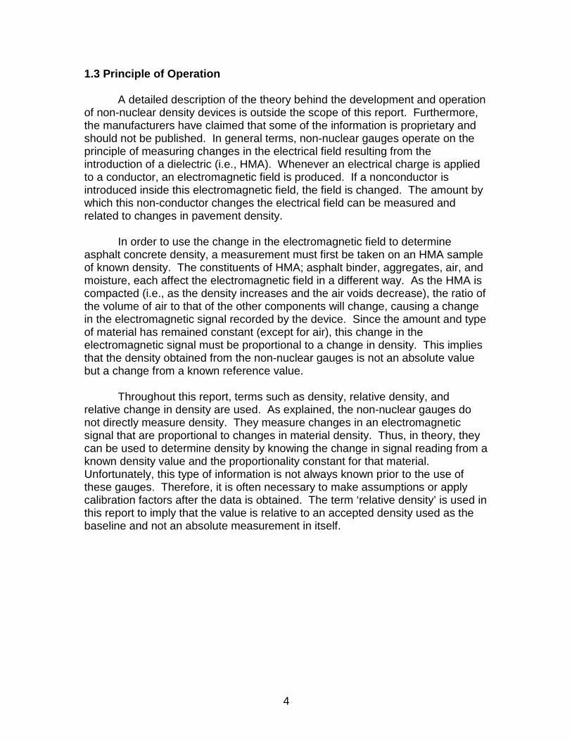
In the summer of 2000, Donald J. Geisel and Associates (Clifton Park, NY) introduced a second non-nuclear density gauge. This second gauge, known as the PaveTracker, is also based on electromagnetic signals but uses different technology. Since this device was also of interest to the HMA paving industry, it was incorporated in the 2001 field study.

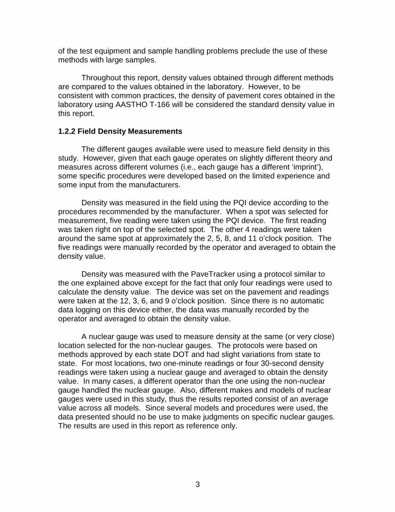
Pictures of the PQI and the Pavetracker are shown in figures 1 and 2,

respectively. 1.2 Density The density of any solid material is defined in AASHTO M132 (ASTM E12) as the mass of a unit volume of material at a specified temperature. However, asphalt concrete is not a completely solid material. The volume used in the calculations contains elements such as discrete solid particles of different sizes (aggregates), semi fluid material (asphalt binder), air (voids), and other materials added to the asphalt concrete (fines). As a result of this, the density measurement is tied to a given volume. In other words, it is possible that a larger or a smaller volume of the same asphalt concrete sample will results in a different density value. Furthermore, it is also possible that an identical volume at a different location within the same material can give a different density value. Within this context, no absolute density value can be defined and some variations in density measurements exist. The acceptable magnitude of this variation depends on the specific application of the measurement (e.g., quality control versus quality assurance). However, regardless of application, the most accepted density value is that obtained from actual samples taken from the pavement and measured in the laboratory using standard procedures such as the ones outlined in AASHTO T-166: Bulk Specific Gravity of Compacted Bituminous Mixtures Using Saturated Surface-Dry Specimens or other suitable variations of this method (e.g. Corelock device). 1.2.1 Laboratory Density Measurements

As was previously stated, the most accepted density value is the one obtained from pavement samples tested in the laboratory. However, there is more than one way to obtain density in the laboratory. For example, by knowing the dimensions of the sample (l x w x h) and its mass, the bulk density can be determined. This assumes smooth surfaces and thus, a small error is introduced in low-density or coarse samples. Another common method to obtain the bulk density is to determine the bulk specific gravity of the sample using the procedure in AASHTO T-166 and multiply this value by the density of water. However, if the percent of water absorbed is high (greater than 2 percent), this method is not recommended. Other methods, such as AASHTO T-275: Bulk Specific Gravity of Compacted Bituminous Mixtures Using Paraffin-Coated Specimens, or the new CoreLock vacuum-sealing device, can be used with high void (high absorption) specimens. Unfortunately, practical limitations on the size

3

of the test equipment and sample handling problems preclude the use of these methods with large samples.

Throughout this report, density values obtained through different methods

are compared to the values obtained in the laboratory. However, to be consistent with common practices, the density of pavement cores obtained in the laboratory using AASTHO T-166 will be considered the standard density value in this report. 1.2.2 Field Density Measurements The different gauges available were used to measure field density in this study. However, given that each gauge operates on slightly different theory and measures across different volumes (i.e., each gauge has a different ‘imprint’), some specific procedures were developed based on the limited experience and some input from the manufacturers.

Density was measured in the field using the PQI device according to the procedures recommended by the manufacturer. When a spot was selected for measurement, five reading were taken using the PQI device. The first reading was taken right on top of the selected spot. The other 4 readings were taken around the same spot at approximately the 2, 5, 8, and 11 o’clock position. The five readings were manually recorded by the operator and averaged to obtain the density value.

Density was measured with the PaveTracker using a protocol similar to

the one explained above except for the fact that only four readings were used to calculate the density value. The device was set on the pavement and readings were taken at the 12, 3, 6, and 9 o’clock position. Since there is no automatic data logging on this device either, the data was manually recorded by the operator and averaged to obtain the density value.

A nuclear gauge was used to measure density at the same (or very close)

location selected for the non-nuclear gauges. The protocols were based on methods approved by each state DOT and had slight variations from state to state. For most locations, two one-minute readings or four 30-second density readings were taken using a nuclear gauge and averaged to obtain the density value. In many cases, a different operator than the one using the non-nuclear gauge handled the nuclear gauge. Also, different makes and models of nuclear gauges were used in this study, thus the results reported consist of an average value across all models. Since several models and procedures were used, the data presented should no be use to make judgments on specific nuclear gauges. The results are used in this report as reference only.

4

1.3 Principle of Operation

A detailed description of the theory behind the development and operation of non-nuclear density devices is outside the scope of this report. Furthermore, the manufacturers have claimed that some of the information is proprietary and should not be published. In general terms, non-nuclear gauges operate on the principle of measuring changes in the electrical field resulting from the introduction of a dielectric (i.e., HMA). Whenever an electrical charge is applied to a conductor, an electromagnetic field is produced. If a nonconductor is introduced inside this electromagnetic field, the field is changed. The amount by which this non-conductor changes the electrical field can be measured and related to changes in pavement density.

In order to use the change in the electromagnetic field to determine asphalt concrete density, a measurement must first be taken on an HMA sample of known density. The constituents of HMA; asphalt binder, aggregates, air, and moisture, each affect the electromagnetic field in a different way. As the HMA is compacted (i.e., as the density increases and the air voids decrease), the ratio of the volume of air to that of the other components will change, causing a change in the electromagnetic signal recorded by the device. Since the amount and type of material has remained constant (except for air), this change in the electromagnetic signal must be proportional to a change in density. This implies that the density obtained from the non-nuclear gauges is not an absolute value but a change from a known reference value.

Throughout this report, terms such as density, relative density, and relative change in density are used. As explained, the non-nuclear gauges do not directly measure density. They measure changes in an electromagnetic signal that are proportional to changes in material density. Thus, in theory, they can be used to determine density by knowing the change in signal reading from a known density value and the proportionality constant for that material. Unfortunately, this type of information is not always known prior to the use of these gauges. Therefore, it is often necessary to make assumptions or apply calibration factors after the data is obtained. The term ‘relative density’ is used in this report to imply that the value is relative to an accepted density used as the baseline and not an absolute measurement in itself.

5

Figure 1 Picture of the Pavement Quality Indicator (PQI) used in the laboratory study.

Figure 2 Picture of the PaveTracker used in the field study

6

2. Laboratory Study

A laboratory study was conducted at the FHWA’s Turner-Fairbank Highway Research Center (TFHRC) in 1999 to evaluate the PQI-300 prior to the field study. The objectives of this study were to: (1) measure the density of laboratory-prepared material using the PQI Model 300 and compare the results with those obtained by traditional methods, and (2) document the conditions under which the device can be operated before proceeding with field trials.

A limited laboratory study was later used to test a prototype PaveTracker

using the same materials described in the following section. All of the measurements were taken and reported by the manufacturer of the device. Other laboratory evaluations of the PaveTracker have been done by outside laboratories (e.g., Pine Instruments Co.). Since these studies were not part of the pooled fund study and to avoid any misrepresentation, those results are not included in this report. 2.1 Materials

The New York State Department of Transportation (NYSDOT) provided the materials used for the laboratory study. Aggregates from three different sources and gradations with three different nominal maximum aggregates sizes were used in this evaluation. While no specific mineral analysis was done on the aggregates, it is believed that the materials used represent a wide enough variety of aggregates used in hot-mix asphalt construction so that the conclusions are applicable to most conditions.

The different aggregates were mixed with an unmodified asphalt binder (PG 64-22) according to established job-mix formulas given by NYSDOT. The different mixes were compacted into slabs using a Linear Kneading Compactor. The slabs had final dimensions of 260-mm wide by 320-mm long with heights varying from 69 mm to almost 90 mm. Since all the slabs contained the same amount of material (by mass), different heights corresponded to different densities. 2.2 Experimental Plan

The laboratory experimental plan consisted of five factors. Each factor looked at a specific ability of the PQI-300 to determine the density of asphalt concrete under controlled conditions. This approach allowed for easy evaluation of each factor. However, it did not allow for any assessment of the interactions that might exist between them (e.g., some gradations might be more susceptible to moisture changes than others). Such interactions could be further evaluated once the importance of the main factors is determined.

7

The factors investigated and the hypotheses used in their evaluation are described next.

Factor 1 – Density: Changes in density of asphalt concrete produced with one aggregate source and one gradation should be proportional to the density measured using the PQI-300 device.

Factor 2 – Nominal Maximum Aggregate Size: Changes in the nominal maximum aggregate size and the respective change in gradation properties can affect the ability of the PQI-300 to determine density of asphalt concrete. Factor 3 – Aggregate Source: Changes in the aggregate source and the respective change in gradation-related properties can affect the ability of the PQI-300 to determine density of asphalt concrete. Factor 4 – Temperature: Changes in temperature can affect the ability of the PQI-300 to determine the relative density of asphalt concrete. The internal algorithms inside the PQI device can account for these effects. Factor 5 – Moisture: Moisture in the asphalt concrete can affect the ability of the PQI-300 to determine the relative density of asphalt concrete. The internal algorithms inside the PQI device can account for these effects.

2.2.1 Experimental Procedures

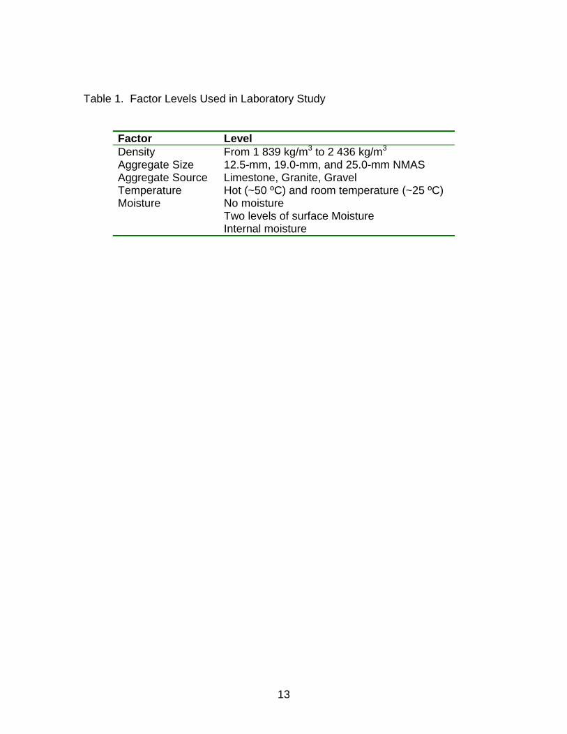
The experimental procedure consisted of making asphalt concrete slabs of ‘known’ density and comparing the accepted density to the density obtained from the PQI-300 when used according to the manufacturer’s instructions. The experimental design for the five factors listed above is shown in table 1. The steps in the experiment are outlined next.

The first step consisted in the compaction of 18 slabs using limestone aggregates having a 12.5-mm nominal maximum aggregate size (NMAS) gradation and a maximum specific gravity of 2.480. Pairs of slabs were compacted to nine different heights ranging from 70.0 mm to 90.0 mm at 2.5-mm intervals.

For the next step, eight slabs were compacted to different heights using the same limestone aggregate but having a 19.0-mm NMAS gradation and a maximum specific gravity of 2.512. The height of these slabs ranged from 69.0 mm to 86.0 mm. This process was repeated with eight more slabs having a 25-mm NMAS gradation and a maximum specific gravity of 2.529. The height of these slabs ranged from 74.0 mm to 91.0 mm.

8

Another set of eight slabs was compacted to different heights using the gravel aggregate with a 12.5-mm NMAS gradation and a maximum specific gravity of 2.430. The height of this slabs ranged from 69.0 mm to 86.0 mm. The process was repeated with eight more slabs using the granite aggregate with a 12.5-mm NMAS and a maximum specific gravity of 2.478. The height of these slabs ranged from 74.0 to 91.0 mm.

Since temperature is known to affect the conductivity of asphalt cement and thus the density readings from the PQI device, the first set of measurements was taken on one side of the slabs after they were compacted, while still relatively hot but out of the mold. This was meant to simulate the field process, where readings are taken during compaction of the hot asphalt pavement mat. The readings were taken using the average mode of the PQI-300 device (i.e., 5 measurements recorded and averaged internally by the device). In as much as possible, the device was moved within the slab to try to capture variations in density from the edge to the center. The data recorded was average density in kg/m3, temperature in degree ºC, and phase angle (a relative measure of moisture, labeled in the PQI display as H2O reading).

The slabs were allowed to cool to room temperature. The PQI-300 was then used in the average mode (as explained earlier) and then in the continuous reading mode (i.e., three individual measurements recorded by the user) to obtain density measurements. During each measurement, the PQI was positioned on a different location throughout the slab. The data recorded in the continuous mode consisted of the density reading, the electrical signal in millivolts (strength of the electrical field measured by the device) and the phase angle (H2O reading). Since the depth of the electrical field is less than the height of the specimens and the density is known to vary with depth, the process was repeated at both the top and the bottom of each slab and the density averaged into one single value.

After all the measurements were taken on the dry slabs, small quantities of surface moisture were applied on one side of each slab using a calibrated spray bottle with water. It was determined that approximately 6 grams of water would coat the surface of the slab. Data was collected using the continuous mode at three conditions: (1) before water was applied, (2) after applying 6 grams of water, (3) after applying 12 grams of water, and, in a few cases, after applying 18 grams of water. This was meant to simulate the condition in which the PQI-300 is used on a mat after a wet roller drives on it and not all moisture has evaporated.

Once the data on surface moisture was collected, the density of the slabs was determined following the procedure in AASHTO T-166, Bulk Specific Gravity of Compacted Bituminous Mixtures Using Saturated Surface-Dry Specimens. This procedure was carried out for two reasons, to obtain an estimate of density (besides mass divided by volume) and to allow water to enter the voids. Some of

9

the water remained in the voids after the slab was submerged and then weighed in the saturated-surface dry condition. Three readings were taken using the PQI-300 on one side of these slabs. These readings were taken to approximate the condition in which internal moisture exists within the pavement. However, it is not clear how closely this last situation represents field conditions.

It is known that the results obtained from the procedure in AASHTO T-166 are not valid when the absorbed water exceeds 2 percent. Thus, to obtain a third estimate of the density (besides mass over volume and AASHTO T-166) the Corelock device was used. For this device to work, the slabs had to be sawn in half. After drying to constant weight, each half was placed inside a plastic bag where the air was removed using the Corelock vacuum. The specific gravity (and the density) was then calculated according to the procedures specified for the Corelock device. The results were consistent with those obtained using mass over volume, thus not reported herein. Attempts to measure slab density using a nuclear density gauge were not successful because the imprint of the nuclear density gauge was bigger than the size of the slabs. Comparisons between the nuclear gauge and the PQI device can be done on the field portion of the study. 2.3 Results

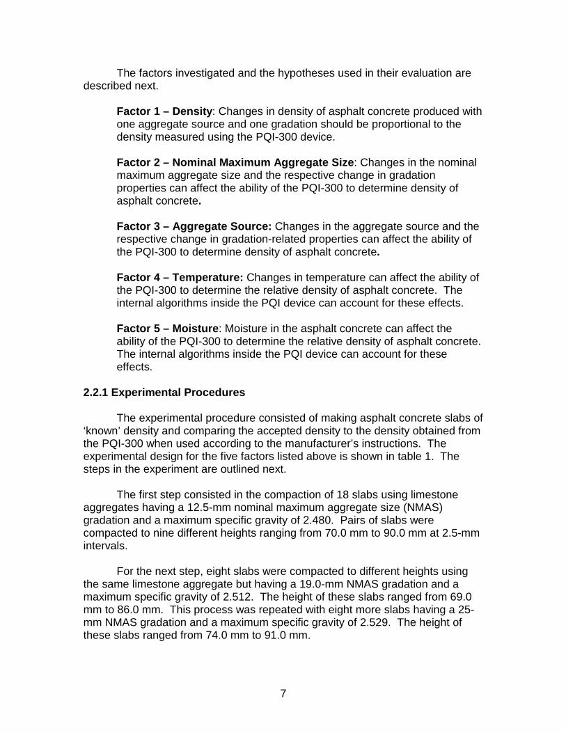
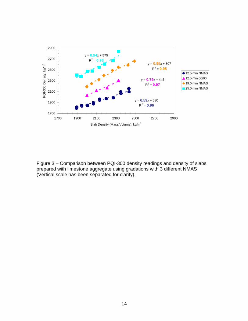
The density of the slabs as measured by the PQI-300 was compared to the density obtained by dividing the mass over the volume (length x width x height). These results are shown in figures 3 and 4. The readings were taken at room temperature on both sides of the slabs (top and bottom) when they were completely dry. Of interest in these figures are the slope of the trend line and the coefficient of determination (R-squared) between both types of measurements. Ideally, both the slope and the R-squared should be close to 1. High values of R-squared would indicate that the PQI density is highly correlated to slab density by a straight line (i.e., slab density can be obtained by multiplying PQI density by a constant). A slope of 1 would indicate that the PQI density exactly matches the slab density at any density level (i.e., there would be no need to determine any constant; it is unity).

Figure 3 shows that the slope for the 12.5-mm NMAS gradation is significantly different than the slopes for the gradations with the larger NMAS (0.59 vs 0.95 and 0.94). This indicates that within one aggregate source and binder type there might be some changes in the dielectric constant. It must be noted, however, that the slabs with the 12.5-mm NMAS gradation were compacted in 1998, while the slabs with the other two gradations were compacted just a few weeks before taking the PQI measurements. This might be an indication of changes in the dielectric constant of the asphalt binder due to oxidative aging. To verify if the differences in the slope were the results of oxidative aging, a new set of slabs was compacted using ‘fresh’ asphalt binder. The data, also shown in figure 3, indicates that indeed, the slope of the relation

10

increases while still showing a high coefficient of correlation. Obviously, one set of data points is not enough to model the effects of aging of the mix. Nevertheless, it points to the fact that the PQI-300 measurements are sensitive to changes in material properties caused by aging.

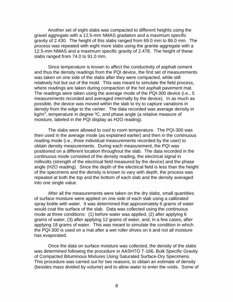
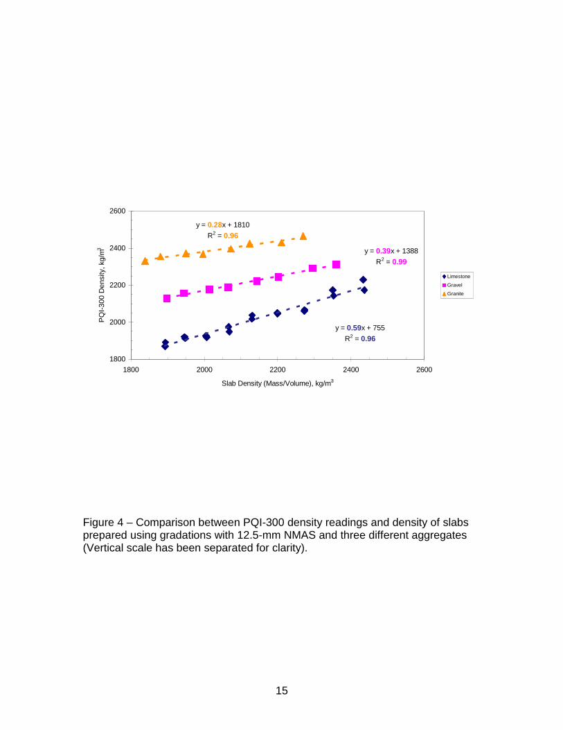
Figure 4 shows the relationship for the three different aggregates

evaluated. The slope of the three lines is different and nowhere near the desired value of 1. This indicates that there is not one unique relationship between PQI density and slab density. Each aggregate (as well as each binder as suspected from the aging results previously shown) has a slope that should be determined individually. Given that each material has its own dielectric characteristics, these results were not unexpected.

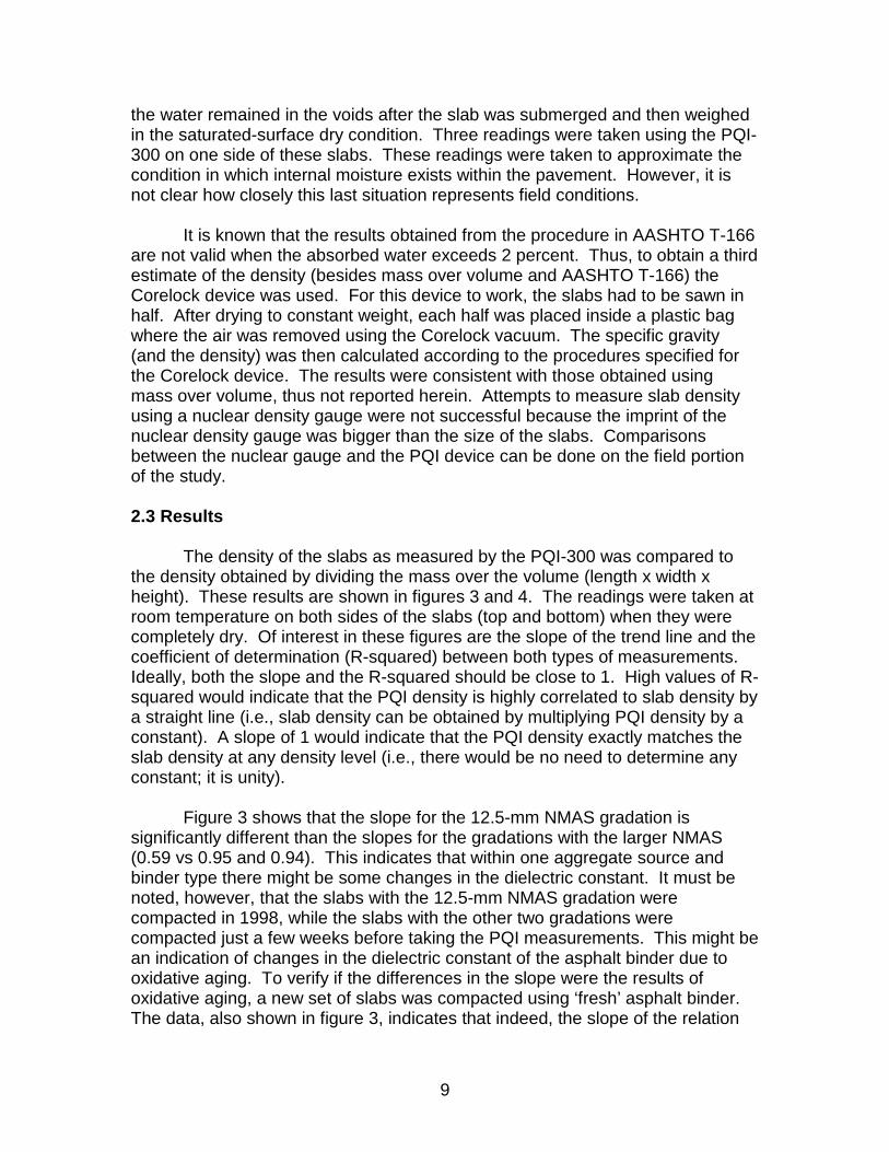
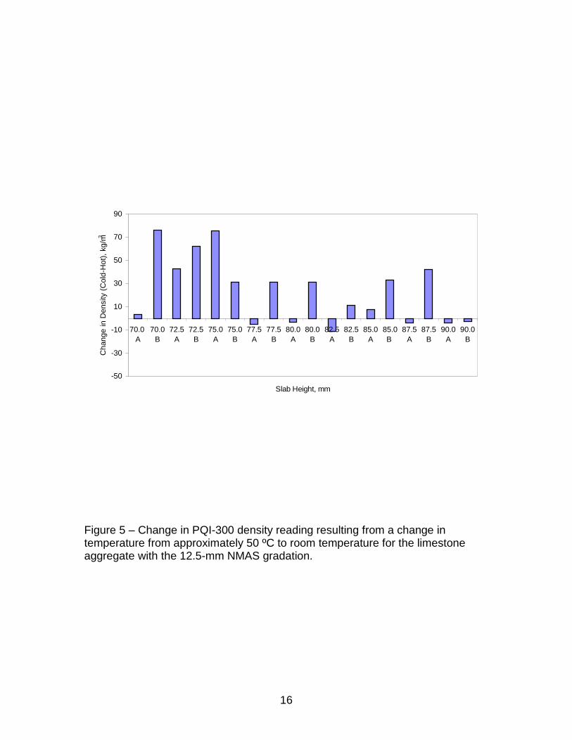
Figure 5 shows how changes in temperature affect PQI density. In most cases, a decrease in temperature caused an increase in PQI density (i.e., the ‘cold’ slabs had higher density). This change was much as high as 70 kg/m3. The temperature of the ‘hot’ slab was between 40 to 60 ºC. This range of temperature is similar to what might be seen in the field after compaction. The ‘cold’ slabs were at room temperature (25 ºC). This resulted in a temperature difference of about 25 ºC between hot and cold measurements. It can only be speculated that if the temperature difference were greater, so would the difference in density readings. As a reference for accepted differences in density measurements, AASHTO T-166 states that, in the laboratory, duplicate specific gravity results should not be considered suspect unless they differ by more than 0.02. If the density of water is taken as 1000 kg/m3, this translates into a difference of 20 kg/m3. Thus, changes caused by differences in temperature can be 2 to 4 times the accepted difference in measurement (note that if AASHTO T-166 were run at a different temperature, the density of water would change so a correction would have to be applied).

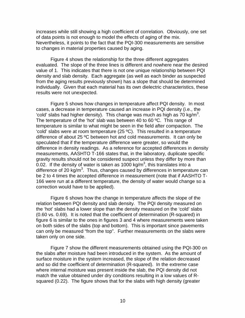
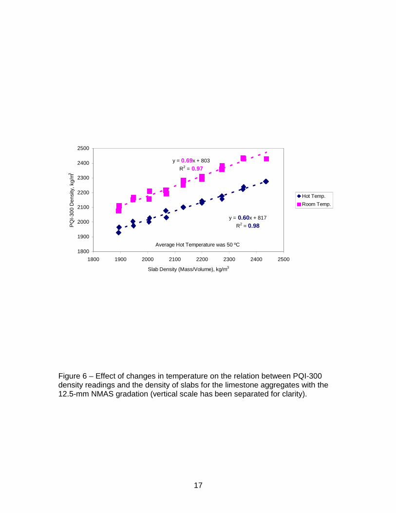
Figure 6 shows how the change in temperature affects the slope of the relation between PQI density and slab density. The PQI density measured on the ‘hot’ slabs had a lower slope than the density measured on the ‘cold’ slabs (0.60 vs. 0.69). It is noted that the coefficient of determination (R-squared) in figure 6 is similar to the ones in figures 3 and 4 where measurements were taken on both sides of the slabs (top and bottom). This is important since pavements can only be measured “from the top”. Further measurements on the slabs were taken only on one side.

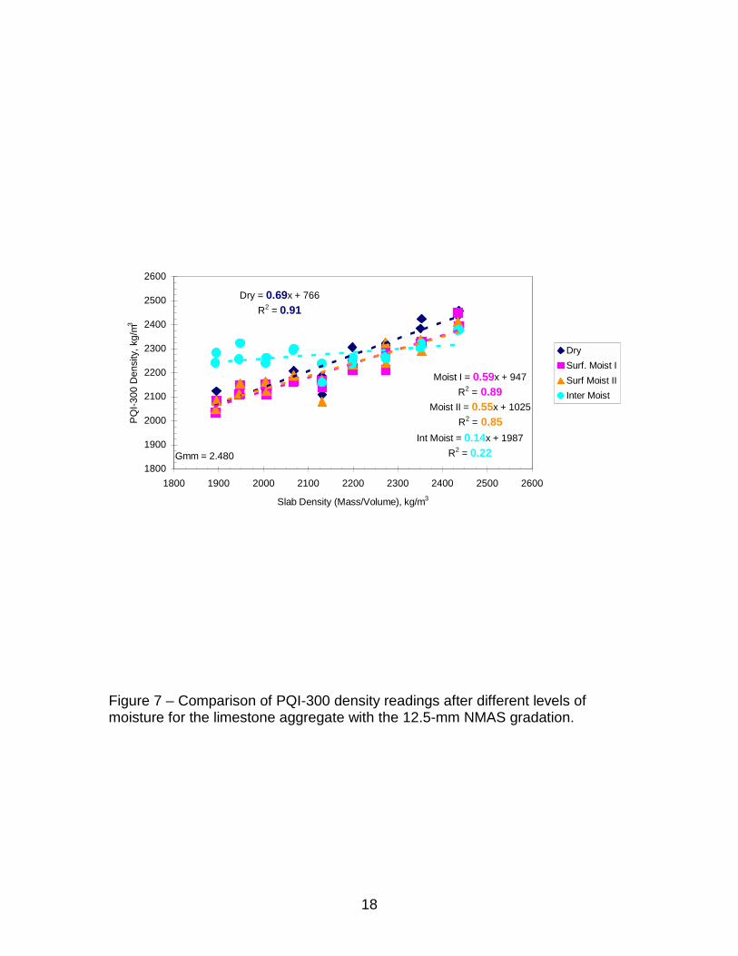
Figure 7 show the different measurements obtained using the PQI-300 on the slabs after moisture had been introduced in the system. As the amount of surface moisture in the system increased, the slope of the relation decreased and so did the coefficient of determination (R-squared). In the extreme case where internal moisture was present inside the slab, the PQI density did not match the value obtained under dry conditions resulting in a low values of R-squared (0.22). The figure shows that for the slabs with high density (greater

11

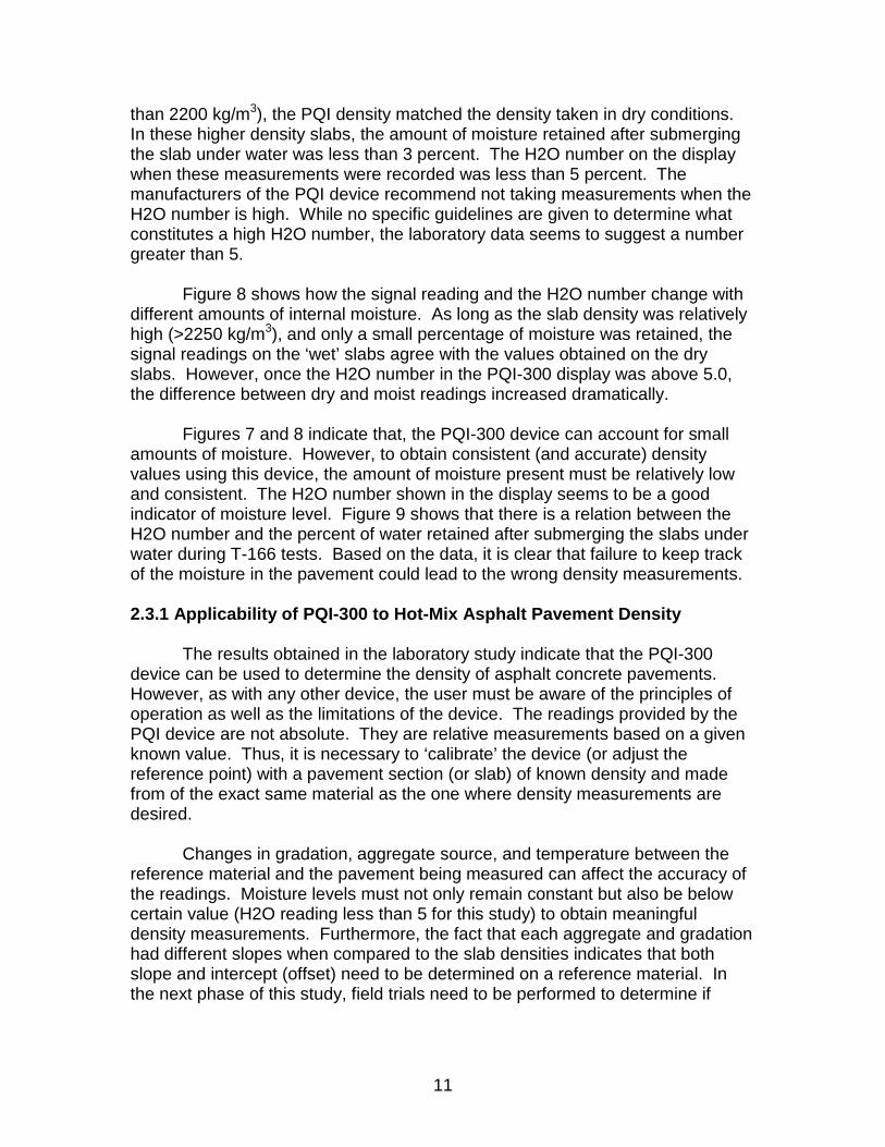
than 2200 kg/m3), the PQI density matched the density taken in dry conditions. In these higher density slabs, the amount of moisture retained after submerging the slab under water was less than 3 percent. The H2O number on the display when these measurements were recorded was less than 5 percent. The manufacturers of the PQI device recommend not taking measurements when the H2O number is high. While no specific guidelines are given to determine what constitutes a high H2O number, the laboratory data seems to suggest a number greater than 5.

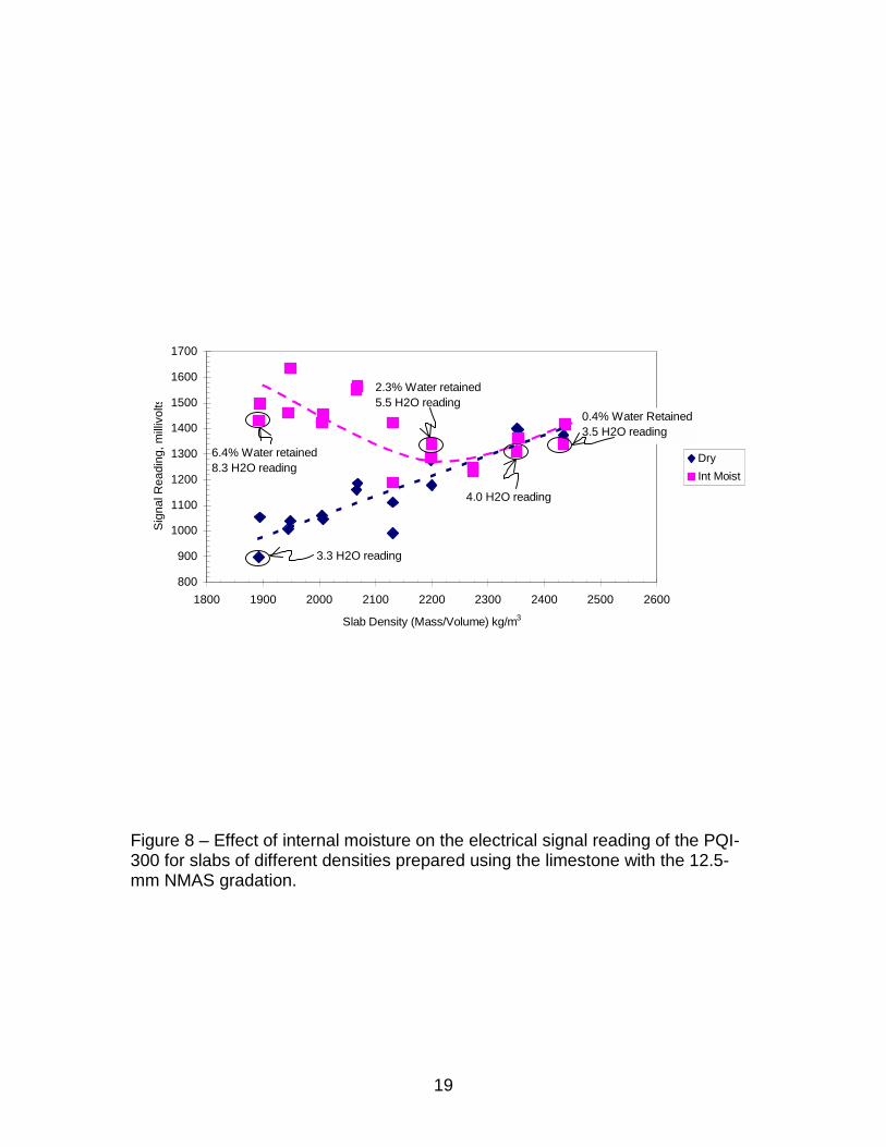
Figure 8 shows how the signal reading and the H2O number change with different amounts of internal moisture. As long as the slab density was relatively high (>2250 kg/m3), and only a small percentage of moisture was retained, the signal readings on the ‘wet’ slabs agree with the values obtained on the dry slabs. However, once the H2O number in the PQI-300 display was above 5.0, the difference between dry and moist readings increased dramatically.

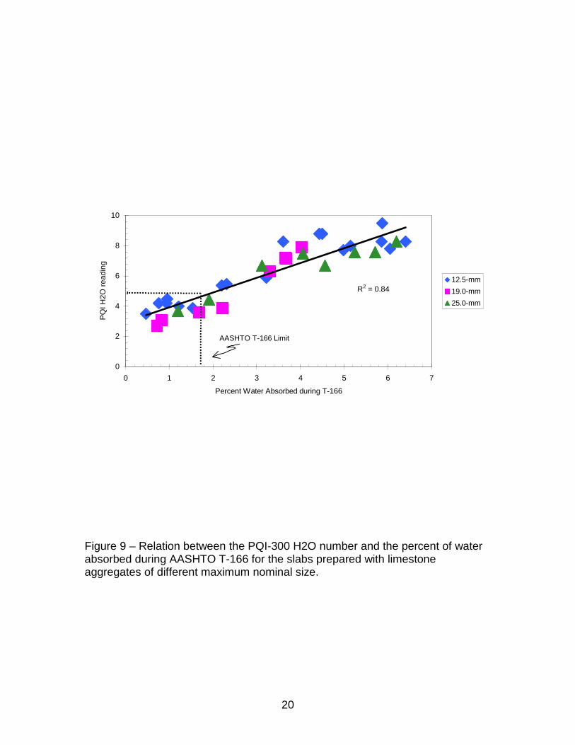
Figures 7 and 8 indicate that, the PQI-300 device can account for small amounts of moisture. However, to obtain consistent (and accurate) density values using this device, the amount of moisture present must be relatively low and consistent. The H2O number shown in the display seems to be a good indicator of moisture level. Figure 9 shows that there is a relation between the H2O number and the percent of water retained after submerging the slabs under water during T-166 tests. Based on the data, it is clear that failure to keep track of the moisture in the pavement could lead to the wrong density measurements. 2.3.1 Applicability of PQI-300 to Hot-Mix Asphalt Pavement Density

The results obtained in the laboratory study indicate that the PQI-300 device can be used to determine the density of asphalt concrete pavements. However, as with any other device, the user must be aware of the principles of operation as well as the limitations of the device. The readings provided by the PQI device are not absolute. They are relative measurements based on a given known value. Thus, it is necessary to ‘calibrate’ the device (or adjust the reference point) with a pavement section (or slab) of known density and made from of the exact same material as the one where density measurements are desired.

Changes in gradation, aggregate source, and temperature between the reference material and the pavement being measured can affect the accuracy of the readings. Moisture levels must not only remain constant but also be below certain value (H2O reading less than 5 for this study) to obtain meaningful density measurements. Furthermore, the fact that each aggregate and gradation had different slopes when compared to the slab densities indicates that both slope and intercept (offset) need to be determined on a reference material. In the next phase of this study, field trials need to be performed to determine if

12

these factors can be controlled and kept constant to obtain actual pavement density.

2.4 Conclusions of the Laboratory Study

Based on the evaluation of the PQI-300 device at the FHWA’s TFHRC using asphalt mixtures with limestone, gravel, and granite aggregates the following conclusions were obtained: 1. Based on the high R-squared values, the PQI-300 device can be used to

determine relative changes in density of asphalt concrete under constant temperature and humidity conditions for a single mixture.

2. Changes in nominal maximum aggregate size produced only small changes in the density relations (slope) between the PQI and the slab density. Thus, it might be possible to use the same proportionality constant (slope) for different aggregate size as long as the same asphalt binder is used.

3. The relationship between PQI readings and density is different for different aggregate sources. It is therefore necessary to calibrate (i.e., determine both slope and offset) the device for individual mixtures.

4. Small amounts of surface moisture in the asphalt concrete do not affect the ability of the PQI-300 device to provide a relative measure of density as long as the moisture remains constant. Thus, determination of any calibration constants must be done under similar moisture levels.

5. The H2O values in the display panel can be used to monitor changes in moisture.

6. High contents of internal moisture continue to provide problems with the density determined using the PQI-300 device. However, the H2O value displayed can be used as an indication of when problems are likely to occur.

2.5 Recommendations From the Laboratory Study

Based on the results obtained in the laboratory study, the following recommendations were made. 1. The slope and intercept need to be determined during calibration. 2. Moisture levels need to be monitored and recorded when measuring density

using the PQI device. 3. Field trials need to be performed to determine if these factors can be

controlled and kept constant to obtain actual pavement density.

13

Table 1. Factor Levels Used in Laboratory Study

Factor Level Density From 1 839 kg/m3 to 2 436 kg/m3 Aggregate Size 12.5-mm, 19.0-mm, and 25.0-mm NMAS Aggregate Source Limestone, Granite, Gravel Temperature Hot (~50 ºC) and room temperature (~25 ºC) Moisture No moisture

Two levels of surface Moisture Internal moisture

14

Figure 3 – Comparison between PQI-300 density readings and density of slabs prepared with limestone aggregate using gradations with 3 different NMAS (Vertical scale has been separated for clarity).

y = 0.59x + 680R2 = 0.96

y = 0.79x + 448R2 = 0.97

y = 0.95x + 307R2 = 0.98

y = 0.94x + 575R2 = 0.93

1700

1900

2100

2300

2500

2700

2900

1700 1900 2100 2300 2500 2700 2900

Slab Density (Mass/Volume), kg/m3

PQI-3

00 D

ensi

ty, k

g/m3

12.5 mm NMAS12.5 mm 06/0019.0 mm NMAS25.0 mm NMAS

15

Figure 4 – Comparison between PQI-300 density readings and density of slabs prepared using gradations with 12.5-mm NMAS and three different aggregates (Vertical scale has been separated for clarity).

y = 0.59x + 755R2 = 0.96

y = 0.39x + 1388R2 = 0.99

y = 0.28x + 1810R2 = 0.96

1800

2000

2200

2400

2600

1800 2000 2200 2400 2600

Slab Density (Mass/Volume), kg/m3

PQI-3

00 D

ensi

ty, k

g/m3

LimestoneGravelGranite

16

Figure 5 – Change in PQI-300 density reading resulting from a change in temperature from approximately 50 ºC to room temperature for the limestone aggregate with the 12.5-mm NMAS gradation.

-50

-30

-10

10

30

50

70

90

70.0 A

70.0B

72.5A

72.5B

75.0A

75.0B

77.5A

77.5B

80.0A

80.0B

82.5A

82.5B

85.0A

85.0B

87.5A

87.5B

90.0A

90.0B

Slab Height, mm

Cha

nge

in D

ensi

ty (C

old-

Hot

), kg

/m3

17

Figure 6 – Effect of changes in temperature on the relation between PQI-300 density readings and the density of slabs for the limestone aggregates with the 12.5-mm NMAS gradation (vertical scale has been separated for clarity).

y = 0.69x + 803R2 = 0.97

y = 0.60x + 817R2 = 0.98

1800

1900

2000

2100

2200

2300

2400

2500

1800 1900 2000 2100 2200 2300 2400 2500

Slab Density (Mass/Volume), kg/m3

PQI-3

00 D

ensi

ty, k

g/m3

Hot Temp.Room Temp.

Average Hot Temperature was 50 ºC

18

Figure 7 – Comparison of PQI-300 density readings after different levels of moisture for the limestone aggregate with the 12.5-mm NMAS gradation.

Dry = 0.69x + 766R2 = 0.91

Moist I = 0.59x + 947R2 = 0.89

Moist II = 0.55x + 1025R2 = 0.85

Int Moist = 0.14x + 1987R2 = 0.22

1800

1900

2000

2100

2200

2300

2400

2500

2600

1800 1900 2000 2100 2200 2300 2400 2500 2600

Slab Density (Mass/Volume), kg/m3

PQI-3

00 D

ensi

ty, k

g/m3

DrySurf. Moist ISurf Moist IIInter Moist

Gmm = 2.480

19

Figure 8 – Effect of internal moisture on the electrical signal reading of the PQI-300 for slabs of different densities prepared using the limestone with the 12.5-mm NMAS gradation.

800

900

1000

1100

1200

1300

1400

1500

1600

1700

1800 1900 2000 2100 2200 2300 2400 2500 2600

Slab Density (Mass/Volume) kg/m3

Sign

al R

eadi

ng, m

illivo

lts

DryInt Moist

3.3 H2O reading

6.4% Water retained8.3 H2O reading

2.3% Water retained5.5 H2O reading

0.4% Water Retained3.5 H2O reading

4.0 H2O reading

20

Figure 9 – Relation between the PQI-300 H2O number and the percent of water absorbed during AASHTO T-166 for the slabs prepared with limestone aggregates of different maximum nominal size.

R2 = 0.84

0

2

4

6

8

10

0 1 2 3 4 5 6 7

Percent Water Absorbed during T-166

PQI H

2O re

adin

g

12.5-mm19.0-mm25.0-mm

AASHTO T-166 Limit

21

3. Field Evaluation Methods

The field evaluation of the non-nuclear gauges was tailored to the specific practices used by each of the participant states. This implied that the selection of test projects, the selection of materials used for comparisons, the number of sites within each project, and the location of each site was determined by each State according to their own established procedures. It was understood that some experimental factors could be confounded if each State followed its own procedures and that, in some cases, not enough data would be available for a rigorous analysis. However, the field evaluation was meant to complement, not duplicate, the laboratory evaluation. Furthermore, by allowing each State to follow its on procedures, more projects could be incorporated and, more importantly, each State would be satisfied that the non-nuclear gauges could be incorporated into their standard procedures to determine pavement density.

3.1 Mathematical Comparisons

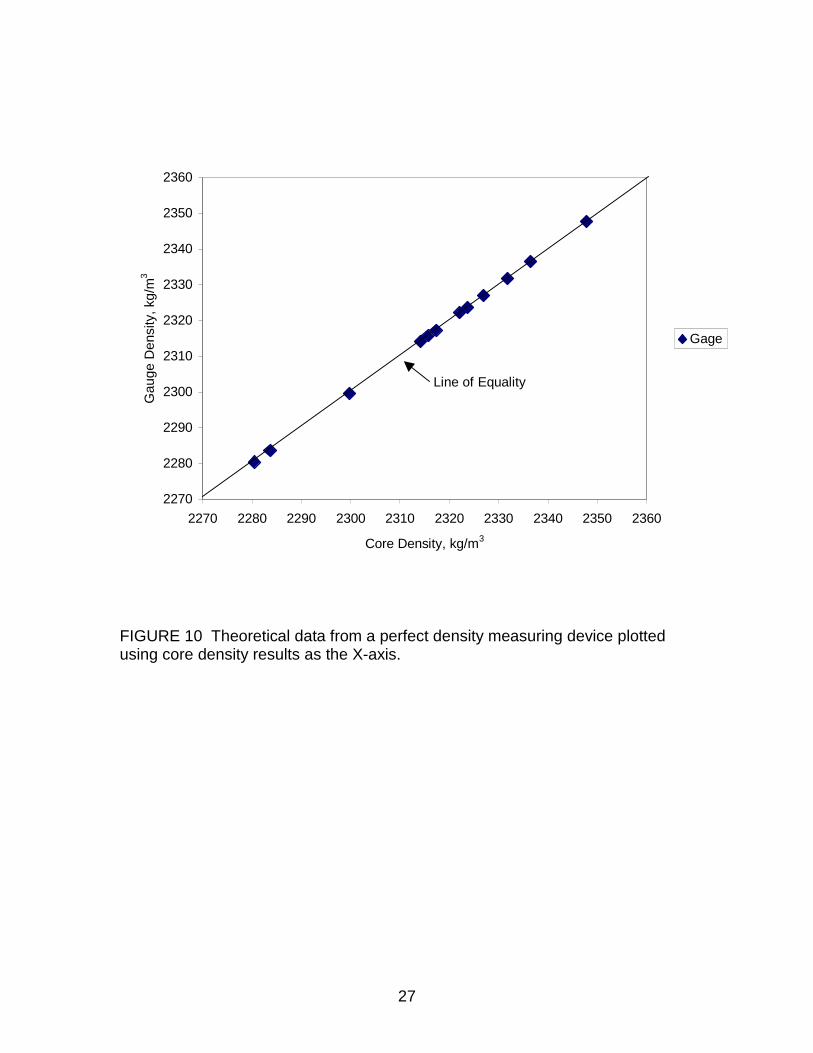
In an ideal situation, the density recorded by any gauge will match the density obtained from the cores. This situation can be visually explained using figure 10. This figure shows that gauge density, when compare against core density, plots along a 45-degree line. In other words, the values obtained from the gauge match the values obtained from the cores and, more importantly, the gauge density can ‘track’ changes in core density (i.e., an increase in core density leads to a proportional increase in gauge density). Unfortunately, in most field experiments the match between gauge density and core density is not perfect. Thus, mathematical parameters must be developed for comparison purposes. Common mathematical methods of comparison are the Student’s t-tests (to test for the difference between measurements taken by two methods or devices) and the coefficient of correlation (to test for the ability of the device to ‘track’ changes in density). Both of these methods have advantages and disadvantages and are described next. 3.1.1. Difference

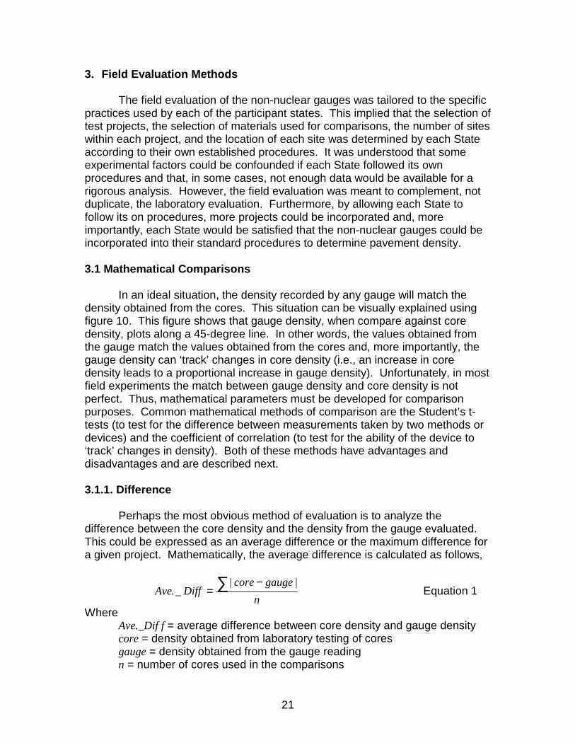
Perhaps the most obvious method of evaluation is to analyze the difference between the core density and the density from the gauge evaluated. This could be expressed as an average difference or the maximum difference for a given project. Mathematically, the average difference is calculated as follows,

ngaugecore

DiffAve ∑ −=

||_. Equation 1

Where Ave._Dif f = average difference between core density and gauge density core = density obtained from laboratory testing of cores gauge = density obtained from the gauge reading n = number of cores used in the comparisons

22

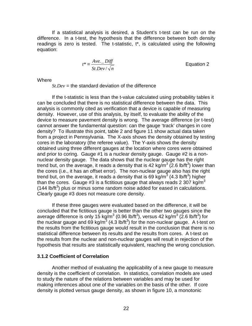
If a statistical analysis is desired, a Student’s t-test can be run on the difference. In a t-test, the hypothesis that the difference between both density readings is zero is tested. The t-statistic, t*, is calculated using the following equation:

nDevStDiffAvet/.

_.* = Equation 2

Where

St.Dev = the standard deviation of the difference

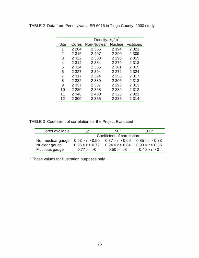
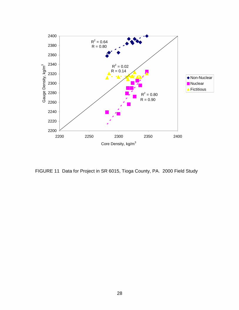
If the t-statistic is less than the t-value calculated using probability tables it can be concluded that there is no statistical difference between the data. This analysis is commonly cited as verification that a device is capable of measuring density. However, use of this analysis, by itself, to evaluate the ability of the device to measure pavement density is wrong. The average difference (or t-test) cannot answer the fundamental question: can the gauge ‘track’ changes in core density? To illustrate this point, table 2 and figure 11 show actual data taken from a project in Pennsylvania. The X-axis shows the density obtained by testing cores in the laboratory (the referee value). The Y-axis shows the density obtained using three different gauges at the location where cores were obtained and prior to coring. Gauge #1 is a nuclear density gauge. Gauge #2 is a non-nuclear density gauge. The data shows that the nuclear gauge has the right trend but, on the average, it reads a density that is 42 kg/m3 (2.6 lb/ft3) lower than the cores (i.e., it has an offset error). The non-nuclear gauge also has the right trend but, on the average, it reads a density that is 69 kg/m3 (4.3 lb/ft3) higher than the cores. Gauge #3 is a fictitious gauge that always reads 2 307 kg/m3 (144 lb/ft3) plus or minus some random noise added for eased in calculations. Clearly gauge #3 does not measure core density.

If these three gauges were evaluated based on the difference, it will be concluded that the fictitious gauge is better than the other two gauges since the average difference is only 15 kg/m3 (0.96 lb/ft3), versus 42 kg/m3 (2.6 lb/ft3) for the nuclear gauge and 69 kg/m3 (4.3 lb/ft3) for the non-nuclear gauge. A t-test on the results from the fictitious gauge would result in the conclusion that there is no statistical difference between its results and the results from cores. A t-test on the results from the nuclear and non-nuclear gauges will result in rejection of the hypothesis that results are statistically equivalent, reaching the wrong conclusion. 3.1.2 Coefficient of Correlation

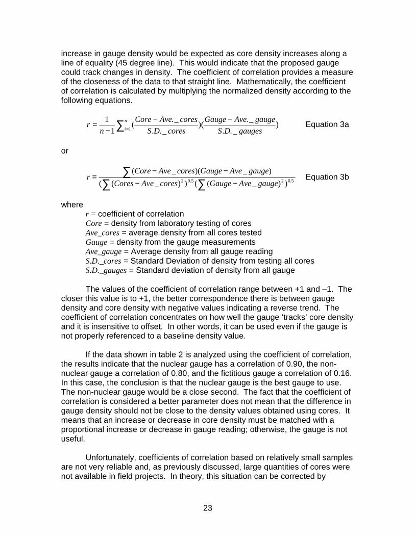
Another method of evaluating the applicability of a new gauge to measure density is the coefficient of correlation. In statistics, correlation models are used to study the nature of the relations between variables and may be used for making inferences about one of the variables on the basis of the other. If core density is plotted versus gauge density, as shown in figure 10, a monotonic

23

increase in gauge density would be expected as core density increases along a line of equality (45 degree line). This would indicate that the proposed gauge could track changes in density. The coefficient of correlation provides a measure of the closeness of the data to that straight line. Mathematically, the coefficient of correlation is calculated by multiplying the normalized density according to the following equations.

)_..

_.)(_..

_.(1

11∑ =

−−−

= n

i gaugesDSgaugeAveGauge

coresDScoresAveCore

nr Equation 3a

or

∑ ∑∑

−−−−

= 5.025.02 ))_(())_(()_)(_(

gaugeAveGaugecoresAveCoresgaugeAveGaugecoresAveCore

r Equation 3b

where

r = coefficient of correlation Core = density from laboratory testing of cores Ave_cores = average density from all cores tested Gauge = density from the gauge measurements Ave_gauge = Average density from all gauge reading S.D._cores = Standard Deviation of density from testing all cores S.D._gauges = Standard deviation of density from all gauge

The values of the coefficient of correlation range between +1 and –1. The

closer this value is to +1, the better correspondence there is between gauge density and core density with negative values indicating a reverse trend. The coefficient of correlation concentrates on how well the gauge ‘tracks’ core density and it is insensitive to offset. In other words, it can be used even if the gauge is not properly referenced to a baseline density value.

If the data shown in table 2 is analyzed using the coefficient of correlation, the results indicate that the nuclear gauge has a correlation of 0.90, the non-nuclear gauge a correlation of 0.80, and the fictitious gauge a correlation of 0.16. In this case, the conclusion is that the nuclear gauge is the best gauge to use. The non-nuclear gauge would be a close second. The fact that the coefficient of correlation is considered a better parameter does not mean that the difference in gauge density should not be close to the density values obtained using cores. It means that an increase or decrease in core density must be matched with a proportional increase or decrease in gauge reading; otherwise, the gauge is not useful.

Unfortunately, coefficients of correlation based on relatively small samples

are not very reliable and, as previously discussed, large quantities of cores were not available in field projects. In theory, this situation can be corrected by

24

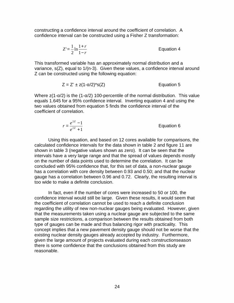
constructing a confidence interval around the coefficient of correlation. A confidence interval can be constructed using a Fisher Z transformation:

rrZ

−+=

11ln

21' Equation 4

This transformed variable has an approximately normal distribution and a variance, s(Z), equal to 1/(n-3). Given these values, a confidence interval around Z can be constructed using the following equation:

Z = Z’ ± z(1-α/2)*s(Z) Equation 5 Where z(1-α/2) is the (1-α/2) 100-percentile of the normal distribution. This value equals 1.645 for a 95% confidence interval. Inverting equation 4 and using the two values obtained from equation 5 finds the confidence interval of the coefficient of correlation.

11

2

2

+−= Z

Z

eer Equation 6

Using this equation, and based on 12 cores available for comparisons, the

calculated confidence intervals for the data shown in table 2 and figure 11 are shown in table 3 (negative values shown as zero). It can be seen that the intervals have a very large range and that the spread of values depends mostly on the number of data points used to determine the correlation. It can be concluded with 95% confidence that, for this set of data, a non-nuclear gauge has a correlation with core density between 0.93 and 0.50; and that the nuclear gauge has a correlation between 0.96 and 0.72. Clearly, the resulting interval is too wide to make a definite conclusion.

In fact, even if the number of cores were increased to 50 or 100, the confidence interval would still be large. Given these results, it would seem that the coefficient of correlation cannot be used to reach a definite conclusion regarding the utility of new non-nuclear gauges being evaluated. However, given that the measurements taken using a nuclear gauge are subjected to the same sample size restrictions, a comparison between the results obtained from both type of gauges can be made and thus balancing rigor with practicality. This concept implies that a new pavement density gauge should not be worse that the existing nuclear density gauges already accepted by industry. Furthermore, given the large amount of projects evaluated during each constructionseason there is some confidence that the conclusions obtained from this study are reasonable.

25

3.2 Effect of Sample Size

It is well established that the density of asphalt pavements is not constant throughout the mat. Also, there are documented variations in the measurement methods used to determine this density (e.g., precision statements in AASHTO T166). Therefore, any density measurement must consider the effect of statistical variations or ‘noise’ in the data. This is normally accomplished by taking a large number of data points. However, as mentioned in the previous section, the amount of cores available for comparisons in some projects was below the desired minimum. The effect of the small sample size was considered by separating the projects into different groups during the 2000 field study.

The projects were separated intro three groups to evaluate the effect of

small sample size. In the first group there were 5 or fewer cores available for comparison. In the second group there were between 6 and 12 cores available for comparison. In the last group there were more than 12 cores available for comparisons. If the small number of cores used in some of the projects had an effect on the conclusions, it would be expected that the results obtained from the table with the least amount of cores available would be very different than the results obtained from the table with the most cores available.

26

TABLE 2 Data from Pennsylvania SR 6015 in Tioga County, 2000 study

Density, kg/m3 Site Cores Non-Nuclear Nuclear Fictitious

1 2 284 2 365 2 194 2 321 2 2 316 2 407 2 290 2 309 3 2 322 2 388 2 290 2 315 4 2 314 2 384 2 279 2 313 5 2 324 2 385 2 301 2 315 6 2 327 2 394 2 272 2 324 7 2 317 2 394 2 256 2 317 8 2 332 2 389 2 306 2 313 9 2 337 2 387 2 296 2 313

10 2 280 2 358 2 239 2 312 11 2 348 2 400 2 325 2 321 12 2 300 2 365 2 236 2 314

TABLE 3 Coefficient of correlation for the Project Evaluated

Cores available 12 50* 100* Coefficient of correlation Non-nuclear gauge 0.93 > r > 0.50 0.87 > r > 0.69 0.85 > r > 0.73 Nuclear gauge 0.96 > r > 0.72 0.94 > r > 0.84 0.93 > r > 0.86 Fictitious gauge 0.77 > r >0 0.50 > r >0 0.40 > r > 0

* These values for illustration purposes only

27

2270

2280

2290

2300

2310

2320

2330

2340

2350

2360

2270 2280 2290 2300 2310 2320 2330 2340 2350 2360

Core Density, kg/m3

Gau

ge D

ensi

ty, k

g/m

3

Gage

Line of Equality

FIGURE 10 Theoretical data from a perfect density measuring device plotted using core density results as the X-axis.

28

R2 = 0.64

R2 = 0.80

R2 = 0.02

2200

2220

2240

2260

2280

2300

2320

2340

2360

2380

2400

2200 2250 2300 2350 2400

Core Density, kg/m3

Gau

ge D

ensi

ty, k

g/m

3

Non-NuclearNuclearFictitious

R = 0.80

R = 0.90

R = 0.14

FIGURE 11 Data for Project in SR 6015, Tioga County, PA. 2000 Field Study

29

4. 2000 Field Study

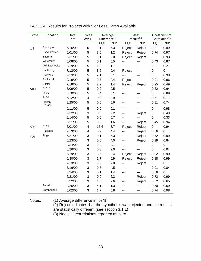
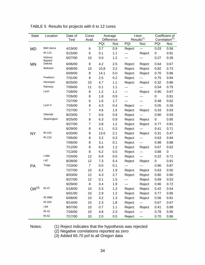
Based on the results of the laboratory study, a field evaluation of the PQI was conducted during the 2000 construction season. The PQI was evaluated using data from 76 projects in six different states, Maryland, Pennsylvania, Connecticut, New York, Minnesota, and Oregon. In each of the projects, density measurements were taken at different locations using both a nuclear gauge and the PQI-300 as explained in section 1.2.2. Following the density gauge measurements, cores were taken and analyzed in the laboratory. The number of cores available for comparisons varied from project to project. Some projects had as little as 3 cores, most have between 5 and 12. Two projects lack enough data for statistical comparisons. A summary of the projects evaluated and the results are shown in tables 4 through 6.

In the state of Oregon, the data was taken in two ways. Sand was used

between the density gauge and the pavement to ensure proper contact and eliminate any irregular seating caused by the rough pavement surface. Measurements were also taken without the sand. The data taken with sand provided slightly better results for all gauges and was used in this report for the analysis.

As explain in section 3.1, two parameters were selected for evaluation, i) the statistical difference as determine by the student’s t-test and ii) the coefficient of correlation between core and gauge density. Since neither parameter, by itself, can be used to evaluate the density gauge, both are presented. 4.1 Results Based on Difference A t-test was conducted to determine if the density obtained using the PQI was statistically different than the density obtained from cores. As explained in section 3.1.1, the hypothesis that the difference between both density values is zero was tested at a 95% confidence level. This resulted in either a rejection of the hypothesis (i.e., the density values are statistically different) or a failure to reject it (i.e., the density values are statistically equivalent). Statistically speaking, failure to reject does not imply acceptance of the hypothesis. In cases where there is large variability in the measurements, a t-test might fail to reject a hypothesis that is false. This is known as type II error and can be determined using a more rigorous statistical analysis. This analysis was not conducted as part of this study. 4.1.1 Analysis

Tables 4 through 6 show the projects analyzed in this study. Those in which the hypothesis was rejected are labeled ‘reject’ indicating that the density obtained from the specific gauge was statistically different that the density obtained from cores.

30

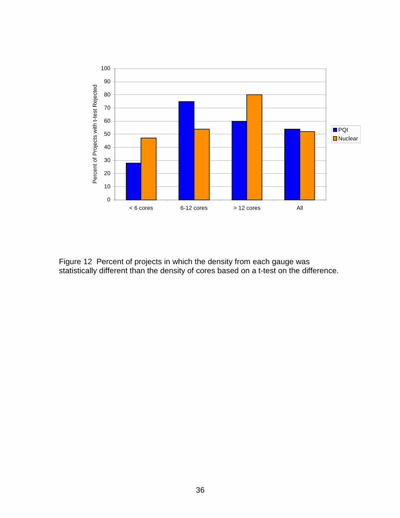
For those projects with 5 or fewer cores available, the PQI-300 gave statistically different density values in 9 out of 32 projects (28%). However, since 14 of the projects in this table only had 3 cores, the results, while encouraging, can be misleading. Analysis of the projects that had between 6 and 12 cores available indicates that the PQI gave statistically different densities in 28 out of 37 projects (75%). For those projects with 15 or more cores available, the hypothesis was rejected in 3 out of 5 projects (60%).

If the results from all projects are combined, the PQI provided density

values that were statistically different from those obtained using cores in 40 out or 74 projects (54%). However, if the results for projects with 6 or more cores are used (tables 5 and 6), in 31 out of 42 (74%) projects the PQI-300 gave statistically different results

The nuclear density gauge did not provide results that were any better. In

39 out of 74 projects (52%) the density from the nuclear gauge was statistically different than the density obtained by analyzing cores in the laboratory.

These results are shown graphically in figure 12.

4.2 Results Based on Correlation The coefficient of correlation was determined between the density obtained from gauge readings and cored samples as explained in section 3.1.2.

The coefficient of correlation obtained in each project was used to compare the performance of the PQI density gauge to the performance of the nuclear gauge. Two criteria were used, i) the number of projects where the gauge performed well, with a coefficient of correlation equal or greater than 0.85; and ii) the number of projects where the gauge did not perform well and resulted in a coefficient of correlation of 0.60 or less. The cutoff values, 0.60 and 0.85, were selected to account for the confidence intervals discussed in section 3.1.2. However, other values were also tried and the conclusions remained the same. Obviously, a value of 0.60 is an unacceptable correlation.

4.2.1 Analysis

Based on the results shown in tables 4 through 6, it seems that the PQI-300 device fails to perform at the same level as the nuclear density gauge. While there are a few projects in which the coefficient of correlation between the PQI-300 and core density was higher than for the nuclear gauge, in the majority of the cases, the nuclear gauge had higher correlation.

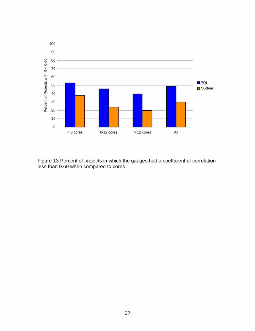
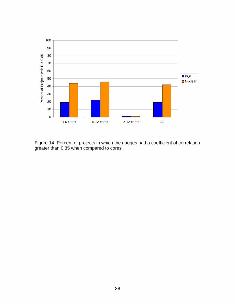
For those projects that had 5 or fewer cores available for comparisons, the PQI had a coefficient of correlation lower than 0.60 in 17 out of 32 projects (53%) and a coefficient of correlation greater than 0.85 in only 6 out of 32 projects

31

(19%). In other words, there were more projects with low coefficient of correlation than projects with high coefficient of correlation. By comparison, the nuclear gauge had a coefficient of correlation lower than 0.60 in 12 out of 32 projects (38%) and a coefficient of correlation greater than 0.85 in 14 out of 32 projects (44%).

For those projects that had between 6 and 12 cores available for

comparisons, the PQI had a coefficient of correlation lower than 0.60 in 17 out of 37 projects (46%) and a coefficient of correlation greater than 0.85 in only 8 projects (22%). Again, similarly to those projects with few cores, there were more projects with low correlation than projects with high correlations. The nuclear gauge had a correlation of less than 0.60 in 9 out of 37 projects (24%) and a correlation greater than 0.85 in 17 out of 37 projects (46%).

For those projects with 15 or more cores available, the PQI did not do any

better. In 2 out of 5 projects (40%) the coefficient of correlation was less than 0.60 while no projects had a coefficient of correlation greater than 0.85. Regardless of the number of cores available for comparisons, there are more projects with low coefficient of correlation than projects with high coefficient of correlation. These results are shown graphically in figures 13 and 14. 4.3 Discussion

Analysis of the data collected indicates that the density obtained from the PQI was statistically different than the core density in 54% of the projects and the PQI density had high correlation to core density in less than 20 percent of the projects. Based on the data shown in tables 4 through 6, the PQI-300 failed to perform at the same level as the nuclear density gauge.

These results were unexpected given the encouraging data obtained in the laboratory. Many factors could have contributed to the poor field performance in the PQI device. Some of the factors might include moisture, temperature during field measurements, and lack of range in the device. Existing algorithms within the PQI-300 device were supposed to correct for these factors; however, the algorithms are based on limited data. Using the vast amount of data collected in this project, updated algorithms needed to be incorporated into the device to improve its performance.

Two issues that were suggested during the laboratory study and might explain the poor results are i) the lack of calibration procedures and ii) the lack of a standard value. Laboratory data showed that it is necessary to adjust both the offset (intercept) and the constant of proportionality (slope) for each mixture. This was seldom performed in the field due to lack of available procedures and data. A calibration standard is also needed to ensure that the PQI is not only

32

reading the correct value but also that different devices give the same answer regardless of the location or operator. 4.4 Summary of Results Based on the data analyzed from 6 different state highway agencies and 76 field projects the following results are obtained:

1- The density obtained using the PQI-300 was statistically different from core density in 54% of the projects.

2- The density obtain from the PQI-300 had a high correlation with core density in 17 percent of the projects.

3- The density obtained from the PQI-300 had low correlation with core density in 60 percent of the projects.

4- The nuclear density gauge did not provide perfect results either. It provided statistically different results in 53% of the projects. However, it had better correlation with core density than the PQI-300.

4.5 Conclusion of the 2000 Study

Based on the results obtained from the 2000 field study, it was concluded that the factors shown in the laboratory study to affect the PQI-300 readings cannot be successfully controlled in the field. The PQI-300 could not be used to measure pavement density with any level of reliability. 4.6 Recommendations

It is recommended that improvement to the PQI-300 algorithms be made and that calibration methods be developed to improve the reliability of pavement density measurements. Until changes are made, it is recommended that the PQI-300 not be used to measure pavement density.

33

TABLE 4 Results for Projects with 5 or Less Cores Available State Location Date

Test Cores Avail.

Average Difference(1)

T-test Results(2)

Coefficient of Correlation(3)

PQI Nuc PQI Nuc PQI Nuc CT Stonington 5/16/00 5 2.1 5.3 Reject Reject 0.81 0.99 Barkhamsted 6/01/00 5 8.5 1.2 Reject Reject 0.74 0.97 Sherman 5/31/00 5 9.1 2.0 Reject Reject 0 0.93 Waterbury 6/08/00 5 0.1 0.5 --- --- 0.43 0.87 Old Saybrooke 6/19/00 5 1.0 1.7 --- --- 0 0.27 Southbury 7/12/00 5 3.6 0.4 Reject --- 0 0 Plainville 9/13/00 5 2.1 0.1 --- --- 0 0.99 Rocky Hill 9/19/00 5 9.7 0.4 Reject --- 0.91 0.96 Bristol 7/18/00 5 2.9 1.4 Reject Reject 0.95 0.49 MD Rt 113 5/09/00 5 0.0 0.5 --- --- 0.62 0.64 Rt 16 5/10/00 5 0.4 0.1 --- --- 0 0.89 Rt 50 5/12/00 4 0.0 2.9 --- --- 0.51 0.11 Hickory

ByPass 8/25/00 5 0.0 0.6 --- --- 0.81 0.74

9/11/00 5 0.0 0.1 --- --- 0 0.98 9/12/00 3 0.0 2.2 --- Reject 0 0.49 9/14/00 5 0.0 0.7 --- --- 0 0.33 9/21/00 5 0.2 1.6 --- Reject 0.45 0.94 NY Rt 15 6/01/00 4 16.6 3.7 Reject Reject 0 0.94 Palisade 9/13/00 4 0.2 4.4 --- Reject 0.66 0 PA Tioga 6/21/00 3 0.1 6.3 --- Reject 0.72 0.99 6/23/00 3 0.0 4.0 --- Reject 0.99 0.84 6/24/00 3 0.9 0.1 --- --- 0 0 6/26/00 3 0.3 2.0 --- --- 0 0.04 6/29/00 3 8.6 2.4 Reject Reject 0.92 0.90 6/30/00 3 1.7 0.9 Reject Reject 0.88 0.99 7/13/00 3 0.3 7.0 --- Reject 0 0 7/16/00 3 0.3 4.5 --- --- 0.91 0.84 6/24/00 3 0.1 1.4 --- --- 0.66 0 6/21/00 3 0.9 6.3 --- Reject 0.72 0.99 6/22/00 3 1.5 7.6 --- Reject 0.02 0.65 Franklin 4/26/00 3 4.1 1.3 --- --- 0.50 0.69 Cumberland 5/02/00 3 1.7 0.8 --- --- 0.74 0.98

Notes: (1) Average difference in lbs/ft3

(2) Reject indicates that the hypothesis was rejected and the results are statistically different (see section 3.1.1) (3) Negative correlations reported as zero

34

TABLE 5 Results for projects with 6 to 12 cores State Location Date of

Test Cores Avail.

Average Difference

t-test Results(1)

Coefficient of Correlation(2)

PQI Nuc PQI Nuc PQI Nuc MD BWI demo 4/19/00 6 3.7 0.9 Reject --- 0.03 0.56 Rt 113 5/15/00 6 0.1 1.1 --- Reject 0 0.91 Hickory

Bypass 9/27/00 10 0.0 1.2 --- --- 0.27 0.26

MN Dakota 6/06/00 8 4.2 2.5 Reject Reject 0.64 0.67 Beltrami 6/08/00 10 10.8 3.2 Reject Reject 0.82 0.73 6/09/00 8 14.1 5.0 Reject Reject 0.70 0.86 Freeborn 7/31/00 8 2.5 0.2 Reject --- 0.75 0.84 Hennepin 8/25/00 10 4.7 1.1 Reject Reject 0.32 0.86 Ramsey 7/09/00 11 0.1 1.1 --- --- 0.54 0.75 Lyon 7/28/00 8 1.2 1.1 --- Reject 0.90 0.97 7/26/00 8 1.8 0.9 --- --- 0 0.91 7/27/00 6 1.6 1.7 --- --- 0.48 0.62 Lyon II 7/26/00 8 4.3 0.4 Reject --- 0.05 0.26 7/27/00 7 4.6 1.5 Reject Reject 0.33 0.93 Ottertail 8/23/00 7 6.6 0.9 Reject --- 0.90 0.93 Washington 9/25/00 8 6.3 0.9 Reject Reject 0 0.95 9/27/00 7 3.8 1.2 Reject Reject 0.77 0.81 9/29/00 8 4.1 0.3 Reject --- 0.41 0.71 NY Rt 415 6/20/00 8 13.0 2.1 Reject Reject 0.31 0.47 Rt 219 7/05/00 8 3.2 0.3 Reject --- 0.63 0.94 7/06/00 8 3.1 0.1 Reject --- 0.98 0.88 7/12/00 8 6.8 1.2 Reject Reject 0.67 0.62 7/13/00 8 6.2 0.5 Reject --- 0.88 0 I-490 7/24/00 12 6.9 0.5 Reject --- 0.22 0.71 I-87 8/28/00 12 7.3 5.4 Reject Reject 0 0.91 PA Tioga 7/10/00 7 0.0 0.1 --- --- 0.96 0.87 7/27/00 10 6.2 1.9 Reject Reject 0.63 0.50 8/03/00 12 4.3 2.7 Reject Reject 0.80 0.90 9/27/00 12 0.1 1.5 --- Reject 0.69 0.53 9/29/00 8 0.4 1.9 --- Reject 0.96 0.72 OR(3) Rt 47 5/18/00 10 0.3 1.3 Reject Reject 0.42 0.54 6/01/00 10 2.9 1.2 Reject Reject 0.77 0.95 Rt 99W 6/08/00 10 3.2 1.3 Reject Reject 0.56 0.81 Rt 204 9/14/00 10 2.3 1.8 Reject --- 0.67 0.67 I-84 9/07/00 10 0.7 1.1 Reject Reject 0.41 0.89 Rt 42 7/26/00 10 4.8 2.3 Reject --- 0.78 0.95 Rt 62 7/17/00 10 2.0 0.5 Reject --- 0.70 0.86

Notes: (1) Reject indicates that the hypothesis was rejected

(2) Negative correlations reported as zero (3) Added 65.70 pcf to all Oregon data

35

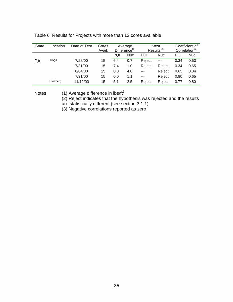
Table 6 Results for Projects with more than 12 cores available State Location Date of Test Cores

Avail. Average

Difference(1) t-test

Results(2) Coefficient of Correlation(3)

PQI Nuc PQI Nuc PQI Nuc PA Tioga 7/28/00 15 6.4 0.7 Reject --- 0.34 0.53 7/31/00 15 7.4 1.0 Reject Reject 0.34 0.65 8/04/00 15 0.0 4.0 --- Reject 0.65 0.84 7/31/00 15 0.0 1.1 --- Reject 0.80 0.65 Blosberg 11/12/00 15 5.1 2.5 Reject Reject 0.77 0.80

Notes: (1) Average difference in lbs/ft3

(2) Reject indicates that the hypothesis was rejected and the results are statistically different (see section 3.1.1) (3) Negative correlations reported as zero

36

0

10

20

30

40

50

60

70

80

90

100

< 6 cores 6-12 cores > 12 cores All

Perc

ent o

f Pro

ject

s w

ith t-

test

Rej

ecte

d

PQINuclear

Figure 12 Percent of projects in which the density from each gauge was statistically different than the density of cores based on a t-test on the difference.

37

0

10

20

30

40

50

60

70

80

90

100

< 6 cores 6-12 cores > 12 cores All

Perc

ent o

f Pro

ject

s w

ith R

< 0

.60

PQINuclear

Figure 13 Percent of projects in which the gauges had a coefficient of correlation less than 0.60 when compared to cores

38

0

10

20

30

40

50

60

70

80

90

100

< 6 cores 6-12 cores > 12 cores All

Perc

ent o

f Pro

ject

s w

ith R

> 0

.85

PQINuclear

Figure 14 Percent of projects in which the gauges had a coefficient of correlation greater than 0.85 when compared to cores

39

5. 2001 Field Study

Based on the results obtained during the 2000 construction season, several recommendations were made to the manufacturer of the PQI device. After some changes were incorporated into the device, including improved algorithms, a field study similar to the one conducted during the 2000 season was initiated in 2001 with participation of 5 different states: Maryland, Pennsylvania, New York, Oregon, and Minnesota. This study also incorporated the PaveTracker as an alternate non-nuclear density gauge.

A total of 38 projects were available for the 2001 field study. The data

was collected in the same manner as explained in section 4. Most projects had 6 or more cores (only 2 projects had less than 6 cores) so the data was not separated into groups as in the 2000 study. Instead tables 7 through 11 show the results for each participant state.

The same evaluation parameters used in the 2000 study were used to

evaluate the performance of the new gauges. 5.1 Results Based on Difference A t-test was conducted to test the hypothesis that the difference between density obtained from each gauge and core density was zero. This is the same analysis done for the 2000 field study and explained in section 3.1.1 5.1.1 Analysis Tables 7 through 11 show that the analysis based on the difference between density values provided similar results as those obtained in the 2000 field study. The hypothesis was rejected for all three gauges evaluated in most of the projects. This is shown graphically in figure 15. While discouraging, this was not an unexpected outcome of the test for reasons explained next. As discussed in section 1.3, the measurements obtained from both the PQI and the PaveTracker are based on relative changes from a known reference value. To actually measure pavement density it is necessary to obtain at least two different measurements at locations with known density. Based on these measurements, the constant of proportionality (slope) and offset (intersect) can be adjusted to the specific materials used in the pavement. This implies that a test section needs to be built in order to measure density with these gauges. Since this is not a practical approach, most users chose to apply arbitrary constants resulting in density values that can be proportional to the real values but are statistically different; as reflected in the data analysis. Of interests in the 2001 study are the results from the state of Pennsylvania, shown in table 9. The PQI-300+ (the + indicates an improved

40

gauge over the regular PQI-300) provided density values that were statistically equivalent to the core density in 6 out of 9 projects (67%) and the PaveTracker in 3 out of 6 projects (50%). This success rate is in contrast to the results from the four other states. It is believed that the reason for these results is the adjustment or calibration done on the field based on their experience using these devices.

These adjustments were done before density values were recorded. A density measurement was taken on the hot-mix asphalt as it came out of the screed. It was assumed, based on their own experience and knowledge of local materials, that the density of the HMA at this location (i.e., prior to any compaction by the rollers) is 87% of the maximum theoretical density of the mixture. Using this number, the gauge was adjusted before any density measurements on the compacted mixture were taken. While these adjustments might be crude, the t-test shows significant improvement in the results by using this approximation. 5.2 Results Based on Correlation The same analysis used in the 2000 field study and discussed in section 4.2 was used in the 2001 study. The comparisons were made on projects with coefficient of correlation greater than 0.85 and projects with coefficient of correlation less than 0.60. Upon inspection of the results, it was noted that there were some projects in which the coefficient of correlation was almost 1 for some gauges but there were a few projects in which the coefficient of correlation was poor for all three gauges (i.e., PQI, PaveTracker, nuclear gauge). Given that it is unlikely that all three gauges failed to perform in a reasonable manner at the same time, it was believed that a mistake was made in measuring density in the cores. As was discussed in section 1.2.1 variations in the density obtained from cores are possible and difficult to control. To avoid any misrepresentation of the gauge performance caused by errors in core density, it was decided to evaluate only projects in which at least one of the three gauges used had a coefficient of correlation greater than 0.75. The projects in which all three gauges had a coefficient of correlation lower than 0.75 are highlighted in the tables and not included in the analysis. 5.2.1 Analysis The results indicate that both the PQI and the PaveTracker have the potential to perform extremely well. As an example, the data from Wolf Road in New York (table 10) shows both gauges with a coefficient of correlation of 0.99. In most states both gauges gave mixed results. However, there was a significant improvement over the 2000 field results.

41

In the state of Maryland the PQI show the worst performance with a coefficient of correlation lower than 0.60 in 2 out of 2 projects evaluated (100%). In contrast, the PaveTracker showed coefficient of correlation greater than 0.85 in 2 out of 3 projects (67%) evaluated. In Minnesota, the PQI had a low coefficient of correlation in 2 out of 5 (40%) projects evaluated and a high coefficient of correlation in 1 out of 5 projects (20%). The PaveTracker had a high coefficient of correlation in 4 out of 7 (57%) projects with no projects showing a low coefficient of correlation.

In the state of Pennsylvania, the PQI showed coefficient of correlation greater than 0.85 in 7 out of 9 (78%) projects and no projects with coefficient of correlation lower than 0.60. The PaveTracker had low coefficient of correlation in 2 out of 5 projects (40%) and high correlation in the same number of projects (40%). In New York, the PQI had high coefficient of correlation in 1 out 6 projects (17%) and low coefficient of correlation in 1 out of 6 projects (17%). The PaveTracker had high coefficient of correlation in 4 out of 6 projects (67%) and low coefficient of correlation in only 1 project (17%). Oregon had only one project evaluated with a coefficient of correlation of 0 for the PQI and 0.79 for the PaveTracker. If the projects from all states are combined, the PQI-300+ had a coefficient of correlation lower than 0.60 in 6 out of 23 projects (26%) and the PaveTracker in 3 out of 22 projects (14%). The PQI had a coefficient of correlation greater than 0.85 in 9 out of 23 projects (39%) and the PaveTracker in 12 out of 22 projects (55%). Both gauges evaluated had more projects with a high coefficient of correlation than projects with a low coefficient of correlation. This was a significant improvement over the 2000 study where the opposite was true. As a reference, the nuclear density gauge had a coefficient of correlation lower than 0.60 in 3 out of 24 projects (12%) and a coefficient of correlation greater than 0.85 in 17 out of 24 projects (71%). These results are shown graphically on figures 16 and 17. 5.3 Discussion The analysis of the data obtained during the 2001 construction season indicates that the density obtained from the PQI was statistically different to core density in 23 out of 34 projects (68%). The density obtained from the PaveTracker was statistically different to core density in 28 out of 34 projects (82%). As discussed in section 5.1.1, the lack of calibration of these devices is believed to be the cause of these results. Significant success was observed in the data from the state of Pennsylvania, where the devices were calibrated based on the experience of the users and knowledge of the local materials.

42

Both non-nuclear gauges had more projects in which the coefficient of correlation was 0.85 or greater (39% for the PQI and 55% for the PaveTracker) than projects in which the coefficient of correlation was 0.60 or less (26% for the PQI and 14% for the PaveTracker. These results indicate that the Pavetracker outperformed the PQI-300+ by a narrow margin but neither gauge was as good as the nuclear gauge. Both non-nuclear gauges had difficulty determining the absolute density of the pavement but were more successful in tracking changes in density. Some users indicated that the non-nuclear gauges were used to identify locations within the pavement with low density. This is perhaps the most significant feature of these devices thanks to their ability to measure relative density in seconds where nuclear gauges usually take minutes. 5.4 Summary of Results Based on the data analyzed from 5 different state highway agencies and 34 field projects the following results are obtained:

1- The density obtained using the PQI-300+ was statistically different from core density in 68% of the projects.

2- The density obtained using the PaveTracker was statistically different from core density in 82% of the projects.

3- The density obtain from the PQI-300+ had a high correlation with core density in 39 percent of the projects.

4- The density obtain from the PaveTracker had a high correlation with core density in 55 percent of the projects

5- The density obtained from the PQI-300+ had low correlation with core density in 26 percent of the projects.

6- The density obtained from the PaveTracker had low correlation with core density in 14 percent of the projects.

7- The nuclear density gauge did not provide perfect results either. The density was statistically different than core density in 75% of the projects. However, it had better correlation with core density than the PQI-300+ or the PaveTracker in most projects.

5.5 Conclusions of the 2001 Study Based on the results of the 2001 field study it was concluded that, in order to use non-nuclear gauges to obtain absolute pavement density, it is necessary to calibrate the devices based on known density values of the same material used in the pavement. Since this is often difficult to accomplish in the field, neither the PQI-300+ nor the PaveTracker are considered suitable to measure pavement density for quality acceptance (QA) purposes or to determine pay factors.

43

However, based on the results and the eased of used, both the improved PQI-300 and the PaveTracker are considered suitable devices for quality control applications to obtain relative pavement density. The immediate feedback provided by both of these gauges can help to identify spots with low pavement density and trigger corrective actions leading to more uniform pavements. 5.6 Recommendations It is recommended that non-nuclear density gauges be used to measure relative density and identify locations within the HMA pavement with low density. It is believed that locations with low density are where future distresses will appear.

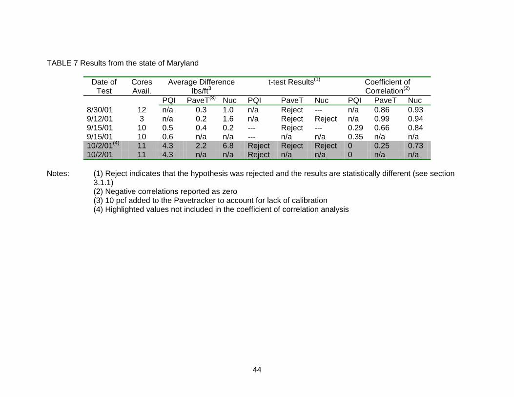
44

TABLE 7 Results from the state of Maryland

Date of Test

Cores Avail.

Average Difference lbs/ft3

t-test Results(1) Coefficient of Correlation(2)

PQI PaveT(3) Nuc PQI PaveT Nuc PQI PaveT Nuc 8/30/01 12 n/a 0.3 1.0 n/a Reject --- n/a 0.86 0.93 9/12/01 3 n/a 0.2 1.6 n/a Reject Reject n/a 0.99 0.94 9/15/01 10 0.5 0.4 0.2 --- Reject --- 0.29 0.66 0.84 9/15/01 10 0.6 n/a n/a --- n/a n/a 0.35 n/a n/a 10/2/01(4) 11 4.3 2.2 6.8 Reject Reject Reject 0 0.25 0.73 10/2/01 11 4.3 n/a n/a Reject n/a n/a 0 n/a n/a

Notes: (1) Reject indicates that the hypothesis was rejected and the results are statistically different (see section

3.1.1) (2) Negative correlations reported as zero

(3) 10 pcf added to the Pavetracker to account for lack of calibration (4) Highlighted values not included in the coefficient of correlation analysis

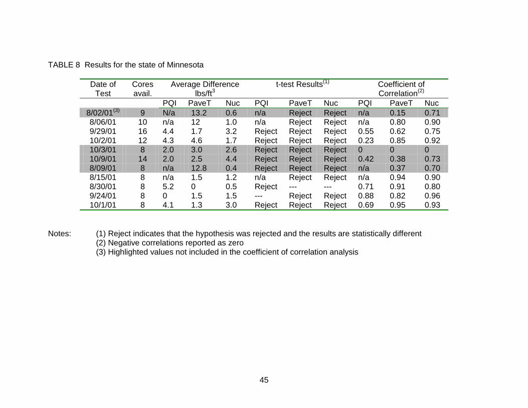
45

TABLE 8 Results for the state of Minnesota

Date of Test

Cores avail.

Average Difference lbs/ft3

t-test Results(1) Coefficient of Correlation(2)

PQI PaveT Nuc PQI PaveT Nuc PQI PaveT Nuc 8/02/01(3) 9 N/a 13.2 0.6 n/a Reject Reject n/a 0.15 0.71 8/06/01 10 n/a 12 1.0 n/a Reject Reject n/a 0.80 0.90 9/29/01 16 4.4 1.7 3.2 Reject Reject Reject 0.55 0.62 0.75 10/2/01 12 4.3 4.6 1.7 Reject Reject Reject 0.23 0.85 0.92 10/3/01 8 2.0 3.0 2.6 Reject Reject Reject 0 0 0 10/9/01 14 2.0 2.5 4.4 Reject Reject Reject 0.42 0.38 0.73 8/09/01 8 n/a 12.8 0.4 Reject Reject Reject n/a 0.37 0.70 8/15/01 8 n/a 1.5 1.2 n/a Reject Reject n/a 0.94 0.90 8/30/01 8 5.2 0 0.5 Reject --- --- 0.71 0.91 0.80 9/24/01 8 0 1.5 1.5 --- Reject Reject 0.88 0.82 0.96 10/1/01 8 4.1 1.3 3.0 Reject Reject Reject 0.69 0.95 0.93

Notes: (1) Reject indicates that the hypothesis was rejected and the results are statistically different

(2) Negative correlations reported as zero (3) Highlighted values not included in the coefficient of correlation analysis

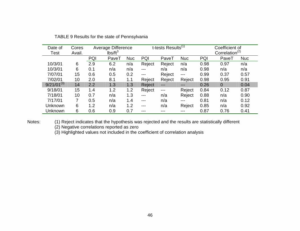
46

TABLE 9 Results for the state of Pennsylvania

Date of Test

Cores Avail.

Average Difference lbs/ft3

t-tests Results(1) Coefficient of Correlation(2)

PQI PaveT Nuc PQI PaveT Nuc PQI PaveT Nuc 10/3/01 6 2.9 6.2 n/a Reject Reject n/a 0.98 0.97 n/a 10/3/01 6 0.1 n/a n/a --- n/a n/a 0.98 n/a n/a 7/07/01 15 0.6 0.5 0.2 --- Reject --- 0.99 0.37 0.57 7/02/01 10 2.0 8.1 1.1 Reject Reject Reject 0.98 0.95 0.91

9/21/01(3) 14 2.2 1.3 1.3 Reject --- --- 0.26 0 0.04 9/18/01 15 1.4 1.2 1.2 Reject --- Reject 0.84 0.12 0.87 7/18/01 10 0.7 n/a 1.3 --- n/a Reject 0.88 n/a 0.90 7/17/01 7 0.5 n/a 1.4 --- n/a --- 0.81 n/a 0.12

Unknown 6 1.2 n/a 1.2 --- n/a Reject 0.85 n/a 0.92 Unknown 6 0.6 0.9 0.7 --- --- --- 0.87 0.76 0.41

Notes: (1) Reject indicates that the hypothesis was rejected and the results are statistically different

(2) Negative correlations reported as zero (3) Highlighted values not included in the coefficient of correlation analysis

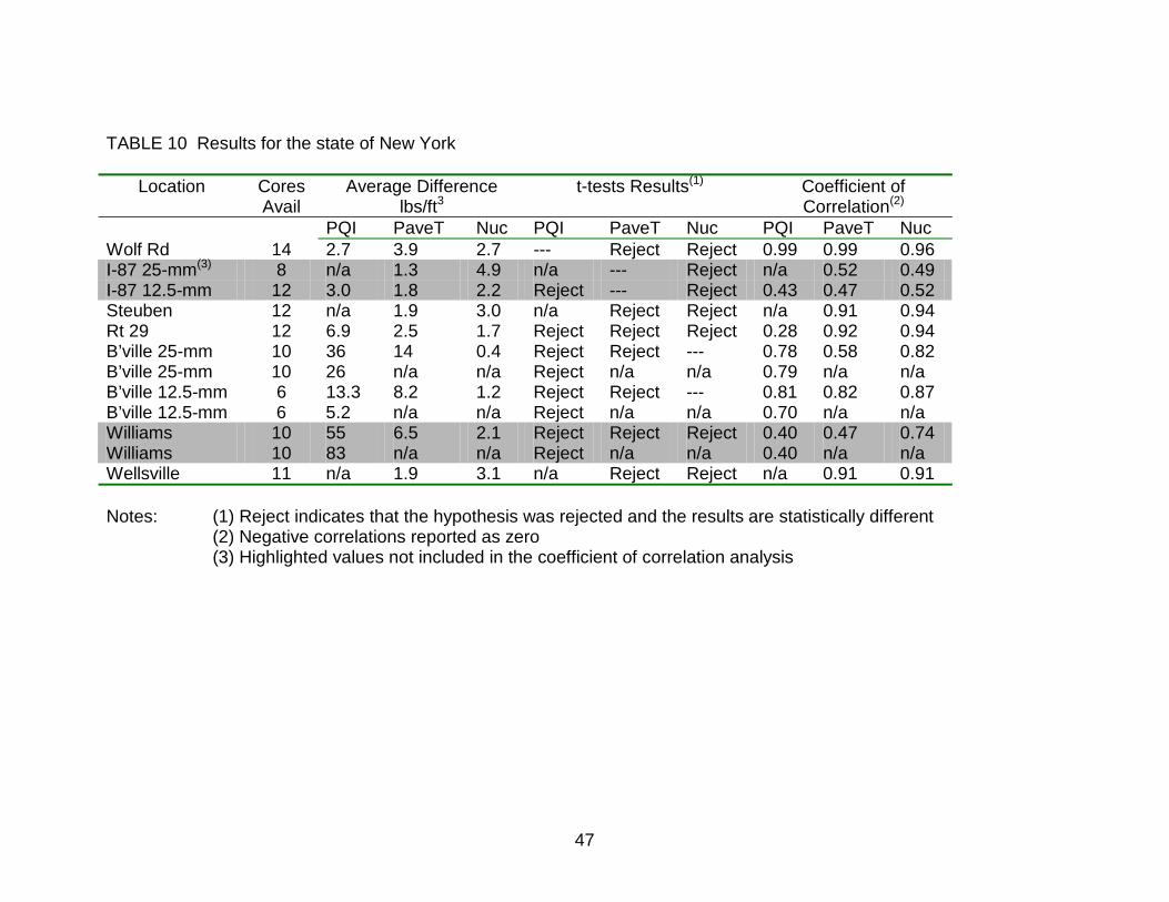
47

TABLE 10 Results for the state of New York

Location Cores Avail

Average Difference lbs/ft3

t-tests Results(1) Coefficient of Correlation(2)

PQI PaveT Nuc PQI PaveT Nuc PQI PaveT Nuc Wolf Rd 14 2.7 3.9 2.7 --- Reject Reject 0.99 0.99 0.96 I-87 25-mm(3) 8 n/a 1.3 4.9 n/a --- Reject n/a 0.52 0.49 I-87 12.5-mm 12 3.0 1.8 2.2 Reject --- Reject 0.43 0.47 0.52 Steuben 12 n/a 1.9 3.0 n/a Reject Reject n/a 0.91 0.94 Rt 29 12 6.9 2.5 1.7 Reject Reject Reject 0.28 0.92 0.94 B’ville 25-mm 10 36 14 0.4 Reject Reject --- 0.78 0.58 0.82 B’ville 25-mm 10 26 n/a n/a Reject n/a n/a 0.79 n/a n/a B’ville 12.5-mm 6 13.3 8.2 1.2 Reject Reject --- 0.81 0.82 0.87 B’ville 12.5-mm 6 5.2 n/a n/a Reject n/a n/a 0.70 n/a n/a Williams 10 55 6.5 2.1 Reject Reject Reject 0.40 0.47 0.74 Williams 10 83 n/a n/a Reject n/a n/a 0.40 n/a n/a Wellsville 11 n/a 1.9 3.1 n/a Reject Reject n/a 0.91 0.91 Notes: (1) Reject indicates that the hypothesis was rejected and the results are statistically different

(2) Negative correlations reported as zero (3) Highlighted values not included in the coefficient of correlation analysis

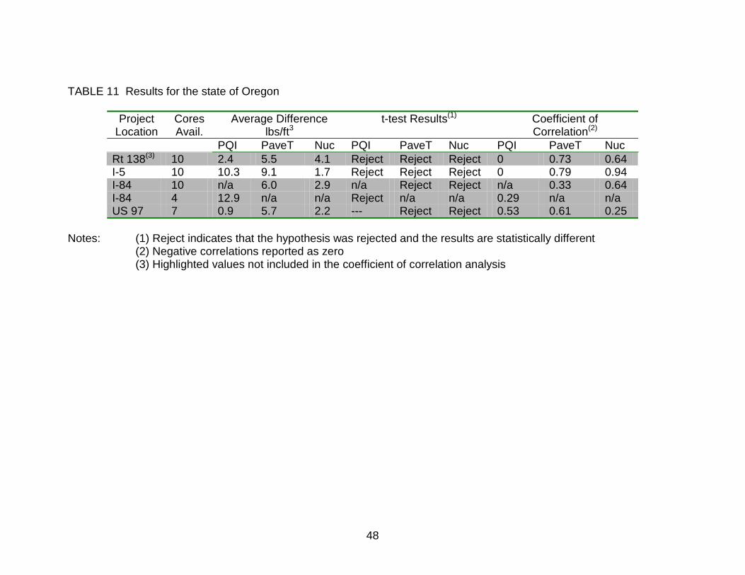
48

TABLE 11 Results for the state of Oregon

Project Location

Cores Avail.

Average Difference lbs/ft3

t-test Results(1) Coefficient of Correlation(2)

PQI PaveT Nuc PQI PaveT Nuc PQI PaveT Nuc Rt 138(3) 10 2.4 5.5 4.1 Reject Reject Reject 0 0.73 0.64 I-5 10 10.3 9.1 1.7 Reject Reject Reject 0 0.79 0.94 I-84 10 n/a 6.0 2.9 n/a Reject Reject n/a 0.33 0.64 I-84 4 12.9 n/a n/a Reject n/a n/a 0.29 n/a n/a US 97 7 0.9 5.7 2.2 --- Reject Reject 0.53 0.61 0.25

Notes: (1) Reject indicates that the hypothesis was rejected and the results are statistically different

(2) Negative correlations reported as zero (3) Highlighted values not included in the coefficient of correlation analysis

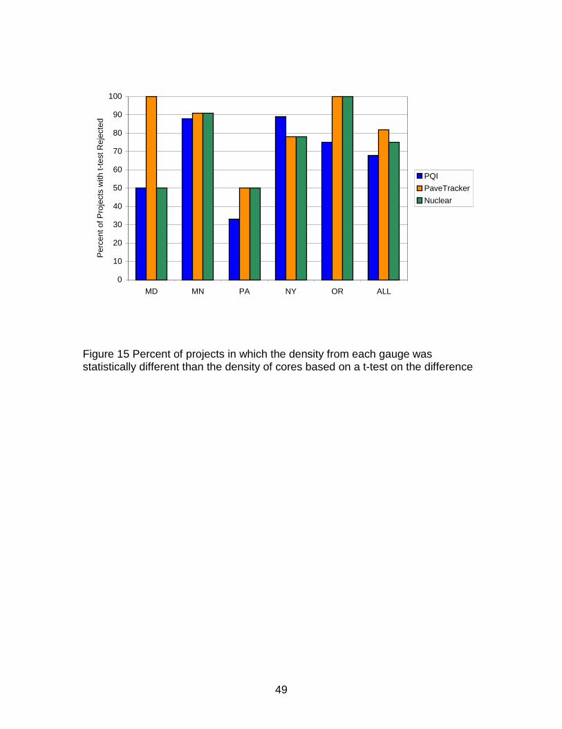
49

0

10

20

30

40

50

60

70

80

90

100

MD MN PA NY OR ALL

Perc

ent o

f Pro

ject

s w

ith t-

test

Rej

ecte

d

PQIPaveTrackerNuclear

Figure 15 Percent of projects in which the density from each gauge was statistically different than the density of cores based on a t-test on the difference

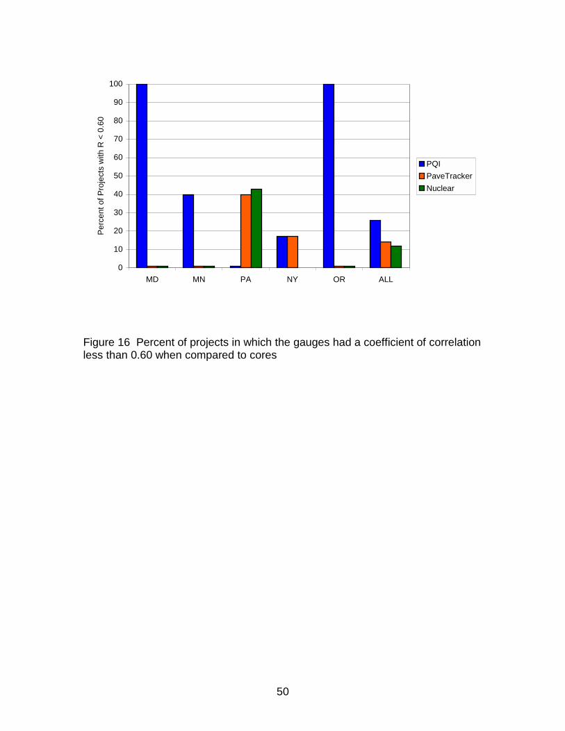
50

0

10

20

30

40

50

60

70

80

90

100

MD MN PA NY OR ALL

Perc

ent o

f Pro

ject

s w

ith R

< 0

.60

PQIPaveTrackerNuclear

Figure 16 Percent of projects in which the gauges had a coefficient of correlation less than 0.60 when compared to cores

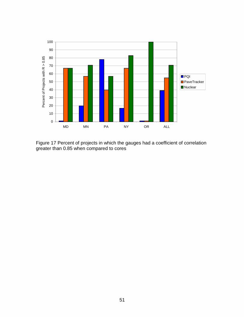
51

0

10

20

30

40

50

60

70

80

90

100

MD MN PA NY OR ALL

Perc

ent o

f Pro

ject

s w

ith R

> 0

.85

PQIPaveTrackerNuclear

Figure 17 Percent of projects in which the gauges had a coefficient of correlation greater than 0.85 when compared to cores

52

6. Evaluation of Gauges Based on Quality Acceptance Specifications

As previously discussed in section 1.2, the measurement of density in HMA pavements carries some variation. The accepted magnitude of this variation depends on the desired application. Throughout this report, analyses between density from gauges and density from cores are made using mathematical relations (discussed in section 3). In this section an attempt is made to quantify the effect of the difference in density measurements caused by the different gauges. This is done using pay factors based on quality acceptance.

If the density of the finished pavement is not within specifications, the

highway agency can assess a penalty that is based on how far the final product is from the target specified density. The pay factor is applied to the cost of the installed asphalt concrete mix. In this section, the criteria used to determine the limits for pay factor determination is listed on table 12, extracted from the American Public work Association (APWA). It presents the limits for pay factor determination based on field density measurements. In this context, using the data collected during two constructions seasons, the effect of the difference in density recorded by the gauges can be assessed in terms of possible penalties. 6.1 Determination of Penalties Caused by Gauge Density The difference in pavement density obtained between cores and the different gauges was evaluated in terms of possible penalties that this difference can lead to. In the analysis, it was assumed that the average maximum theoretical specific gravity of the mixtures (Gmm) was 2.404 for a maximum theoretical density of 150 lbs/ft3. Using this value, the target density value for 95% compaction is 142.5 lbs/ft3. Based on the values shown in table 12, the limits in density are 93% and 97% of Gmm, or 139.4 and 145.5 lbs/ft3, respectively. This implies that there can be a difference in density of ± 3 lbs/ft3 (145.5 – 142.5) with no penalty assessed. In other words, it is assumed that the core density is both correct and on target and any deviations are caused by difference in gauge reading. Under these circumstances, an average gauge error less than 3 lbs/ft3 is of no consequence to the user. The average difference in density shown in tables 4 through 6 and 7 through 11 was separated into two categories and shown in table 13. Using this data, the possible cost of using each gauge was determined. 6.1.1 Results The data from the 2000 study suggests that the error caused by the PQI-300 could lead to a 0.8 pay factor in 43% of the projects. Based on the assumption that the cores are both correct and on target, his implies that the user would get 91.4% of pay at the end of the season (0.8*43 + 1.0*57) if the pay

53

factor is determined based the PQI-300 alone. By contrast the nuclear gauge could lead to a 0.8 pay factor in 18% o f the projects. The total pay at the end of the season is expected to be 96.4%. The data from the 2001 study yielded similar results. The PQI-300+ could lead to a 0.80 pay factor in 45% of the projects. The PaveTracker would lead to a 0.80 pay factor in 39% of the projects and the nuclear gauge in 17% of the projects. Based on these numbers, the total pay in 2001 would be 91.0 % for the PQI-300+, 92.2% for the Pavetracker, and 96.6% for the nuclear gauge. 6.2 Discussion The above analysis is very simplistic and is only meant to illustrate the possible cost of the error introduced by using density gauges for quality acceptance. Obviously, proper calibration as discusses in section 5.1.1 can greatly improve the results. Nevertheless, an assessment can be made of the cost incurred in determining the pavement density using the gauges only and compare that value to the cost of coring and patching the pavement or the cost associated from other methods to measure density (e.g., licensing, training). The PQI will results in a reduction of pay of 9% (100 – 91); the PaveTracker in a reduction in pay of 7.8%; and the nuclear gauge in a reduction of pay of 5.4%.

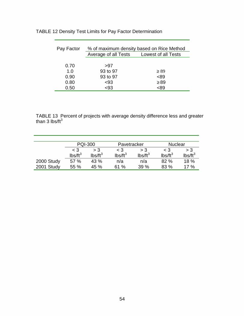
54

TABLE 12 Density Test Limits for Pay Factor Determination

% of maximum density based on Rice Method

Pay Factor

Average of all Tests Lowest of all Tests

0.70

>97

1.0 93 to 97 89≥ 0.90 93 to 97 <89 0.80 <93 ≥ 89 0.50 <93 <89

TABLE 13 Percent of projects with average density difference less and greater than 3 lbs/ft3 PQI-300 Pavetracker Nuclear < 3

lbs/ft3 > 3

lbs/ft3 < 3

lbs/ft3 > 3

lbs/ft3 < 3

lbs/ft3 > 3

lbs/ft3 2000 Study 57 % 43 % n/a n/a 82 % 18 % 2001 Study 55 % 45 % 61 % 39 % 83 % 17 %

55

7. Summary

A study was conducted over 2 construction seasons to assess the applicability of non-nuclear density gauges in pavement applications. Two commercially available gauges were evaluated, the Pavement Quality Indicator (PQI) and the PaveTracker. Throughout the course of this study, both devices underwent significant improvements and open ideas for new applications in pavement construction. There is no doubt that, as a result of this study, more improvements will be incorporated into these devices and, perhaps, other devices will enter the market.

7.1 Conclusions

The density of hot mix asphalt when placed on the road is one of the most critical parameters to control its quality. None of the devices evaluated provided a consistent alternative to taking cores. However, all of the devices show the potential to supplement density measurements in the field.

Based on the results obtained in this study, the following conclusions are

reached 1. Both the Pavement Quality Indicator (PQI) model 300+ (the plus

indicates changes made after the 2000 construction season) and the PaveTracker are suitable devices to control density of hot-mix asphalt during construction. Both devices can provide immediate feedback so that irregular spots can be located and corrective actions taken.

2. Even though neither the PQI-300+ nor the PaveTracker is as accurate as existing nuclear gauges, the advantage of not dealing with regulations associated with the radioactive source of nuclear gauges and the ability to take multiply measurement in shorts periods of time makes them attractive devices for quality control of pavement density during construction.

3. The PQI and PaveTracker must be used by experience operators according to the manufacturers recommendations. While no official certification is required to use these devices, lack of proper training could lead to irregular density measurements.

4. Calibration of these devices to local materials and conditions is critical to obtain accurate results. Whenever practical, the calibration should be done using a test section. However, assumptions made based on knowledge and experience of local materials can greatly improve the results.

5. The only accurate method to obtain absolute pavement density for acceptance or pay factor determination is by taking cores and analyzing them in the laboratory.

56

7.2 Recommendations The following recommendations are made based on the experience obtained from using the non-nuclear density gauges during laboratory and field evaluation.

1. Standard procedures in the form of a specification need to be developed for the use of non-nuclear density devices. The specification should include operating procedures as well as calibration methods. A sample method is included in appendix A.

2. A reference standard, similar to the one used by the PaveTracker should be developed for the PQI device. This reference standard can ensure that the device is working properly prior to use and can alert the operator of possible malfunctions.

3. The practice of measuring density at selected random spots only should be evaluated since this devices can take multiple measurements in short periods of time, thus allowing for more measurements at more locations.

4. Alternative uses for the non-nuclear density gauges should be sought. The ability to take multiple measurements in just seconds combined with their lightweight and portability makes them ideal devices to evaluate the uniformity of pavements. This includes detection of segregated, non-uniform, areas.

57

Appendix A Preliminary Standard Specification

A standard specification or test method developed by Pennsylvania Department of Transportation (PennDOT) is included as a guide for other users to develop a method of their own. This test method can also form the bases for a standard specification developed through the American Society of Testing and Materials (ASTM) or the Association of American State Highway Transportation Official (AASHTO).

While this method was developed specifically for the Pavement Quality

Indicator, it can be easily modified to make generic references to other non-nuclear density gauges including the PaveTracker.

58

Commonwealth of Pennsylvania PA Test Method No. 403 Department of Transportation June 2000

5 Pages

MATERIALS AND TESTING DIVISION Method of Test for

DETERMINING IN-PLACE DENSITY OF BITUMINOUS CONCRETE USING ELECTRICAL IMPEDANCE MEASUREMENT METHODS

1.0 Introduction and Scope

1.1 This test method describes the procedures for determining the in-place density of bituminous concrete by the electrical impedance measurement methods.

2.0 Significance and Applicability

2.1 The test method described is useful as a rapid nondestructive technique for determining the in-place density of compacted bituminous mixtures.

2.2 The density results obtained by this test method are relative,

and require calibration with a known density sample of the material being measured to obtain density readout in absolute numerical values. This is done by calibrating the unit with one or more alternative density measurement procedures in accordance with Section 5 of this standard. 3.0 Interferences

3.1 The mix composition of the bituminous asphalt material being

tested may significantly affect the measurements. The instrument should be calibrated to that specific mix design being used in the field.

3.2 This test method exhibits spatial bias in that the instrument is

most sensitive to the density of the material in closest proximity to the center of the instrument sensor. Oversize aggregate particles in the center of the sensor path may cause variations in density readings. The average of at least 5 readings at different points in close proximity are therefore recommended in accordance with Section 7.0.

3.3. The surface texture of the material being tested may cause

lower than actual density readings. The average of at least 5 readings at

59

different points in close proximity are therefore recommended, in accordance with Section 7.0. 4.0 Apparatus

4.1 The density gauge shall be the Pavement Quality Indicator,

manufactured by Transtech Systems, Inc. or approved equal meeting the requirements outlined below.

4.2 The density gauge shall use a low voltage, alternating

frequency sensing circuit, combined with an impedance sensing head of coplanar design.

4.3 The gauge shall employ suitable electronic circuitry to provide

power and signal conditioning to the sensor to provide the data acquisition and readout function, and allow calibration of the unit over the expected range of application conditions and materials.

4.4 The gauge shall include the internal circuitry suitable for

automatically averaging a number of individual measurements to obtain a mean value.

4.5 The gauge shall include a continuous reading mode of

operation.

4.6 The gauge shall be portable and shall be housed in an enclosure of heavy-duty construction, and designed for taking in situ density measurements of bituminous concrete pavements. 5.0 Calibration

5.1 Calibrate the gauge for each mix design prior to performing

tests on materials that are different from the material types used in establishing the most recent gauge calibration. Calibrate a newly acquired gauge or a repaired gauge.

5.2 Calibrate the gauge in accordance with the manufacturer’s

recommended procedures for the unit. The following general procedures shall also be applicable.

Since the density gauge is designed for typical ranges of asphalt densities, typically only the gauge offset setting will need to be changed to calibrate the instrument to the specific pavement being measured. The gauge slope (sensitivity or gain) will generally not require major adjustment, if any. When applying the unit to different asphalt mix types or conditions, simply changing the offset to correspond to a known density

60

value (close to the optimum density required in the job) will usually yield acceptable accuracy.

5.3 The following general procedure should be followed for gauge

calibration, when in situ pavement sections are utilized.

5.4 The density gauge should be calibrated on the asphalt mat when the temperature of the mat is in the range of temperatures at which subsequent readings will be taken as paving progresses. For gauge calibration using core samples, follow the procedure below and refer to the diagram provided at the end of this PTM.

1. Identify a minimum of 5 test locations within a 10 foot length (in the

direction of traffic) on the asphalt mat. 2. Place the instrument on the asphalt mat at one of the test locations

and draw a circle around the probe of the unit. 3. Using a clockwise rotation record a minimum of 5 single shot

readings, with the instrument, one within the drawn circle, and the other four around the center, moving the instrument at least 2" between readings.

4. Record the readings. 5. Cut a 6" core from the center of the marked circle. 6. Repeat this process at the four additional test locations. 7. In the laboratory, perform the density measurements on the 6"

cores in accordance with PTM 715 and PTM 716 and record the results.

8. Compare the readings obtained with the instrument with the core densities.

9. Note the numeric difference between the average density values of the instrument to the core density.

10. Add or subtract the numeric difference from the offset number found in the instrument. This will calibrate the instrument to the asphalt mat by adding (or subtracting) the average numeric difference from Step 8 to the offset number on the gauge.

5.5 All data used for calibration shall be recorded on the “Report on Compaction Density By Electrical Impedance Measurement Method” form.

6.0 Test Site Preparation

6.1 Since surface conditions can have a significant effect on density

measurements, a dry, smooth surface is required for proper testing. The optimum condition for testing would be a completely dry, smooth surface, with total contact between the bottom surface of the gauge and the surface being tested.

61

6.2 Select a flat, relatively smooth test area on the bituminous mat. Dry the area to be measured with an absorbent cloth to remove any standing water and brush the surface clear of any sand or stones which would prevent intimate contact between the surface and the gauge.

7.0 Procedure

7.1 Ensure that the unit is calibrated in accordance with Section 5.0 of this

specification for the site conditions and bituminous mix being used.

7.2 Seat the gauge firmly on the test surface (prepared in accordance with this specification). Locate the measurement area away from any known sources of electromagnetic interference such as overhead high tension powerlines or large metal objects. 7.3 Place the instrument on the asphalt mat and trace a circle around the probe (base) of the unit. 7.4 Record a minimum of 5 single shot readings with the instrument beginning with a reading at the center and moving clockwise around the center moving the instrument at least 2" between readings as shown in Appendix A. 7.5 Average the readings taken at the 5 individual locations to obtain an average density value. 7.6 Record data in accordance with Section 8.0 of this standard. 8.0 Recording Results.

8.1 Immediately after taking the density readings record the following data on the

“Report on Compaction Density By Electrical Impedance Measurement Method” (Appendix A1) upon taking the density readings. Minimum data to be reported include the following:

1. Job site identification and test site location data in accordance with standard contractor protocols.

2. Gauge calibration data as specified in Section 5.0.

3. Individual readings of the density gauge at each measured point within a

test location, together with the calculated average density value for the location.

4. Corresponding density data (if taken) from alternative methods for each

test location. Such data may be from nuclear gauge or core sample methods, in accordance with PTM 402, PTM 715, PTM 716.

PTM No. 403 June 2000

Page 62

62

5. Notation of any qualitative observations of testing or material conditions

which may affect the accuracy or interpretation of test results. 6. Temperature of the bituminous mat at the time of readings, if taken.

7. Dated signature by the test operator.

PTM No. 403 June 2000

Page 63

63

APPENDIX A1 REPORT ON COMPACTION DENSITY

BY ELECTRICAL IMPEDANCE MEASUREMENT METHOD (Reference P.T.M. 403)

Fill out Completely, Retain original with project records, Mail copy to District. S.R.__________ Sec.__________ County__________ District___________ Date__________ Project No.__________________Contractor_____________________________________________ Mix Description________ Mat thickness______ Compaction Targets ____%min. to ____%max Technician Name___________________________ Testing Company_____________________ Gauge Settings: Maximum Theoretical Density_________ Offset_________ Slope________ Test No.

Sta Offset Single Read 1

Single Read 2

Single Read 3

Single Read 4

Single Read 5

Single Read Avg.

Avg. Mode Read

Nucl. #1 __sec

Nucl. #2 __sec

Core Data

Remarks

Signature of Gauge Operator___________________ DATE _______________

64

Appendix B Alternate Evaluation of 2001 Field Data The data from the 2001 field study was analyzed by Professor Eyad Masad from Washington State University. The results are presented in this section.

Statistical Analysis of Asphalt Pavement Density Measurements

A Report Prepared by

Dr. Eyad Masad

1330 SW Wadleigh Drive Pullman, WA 99163

Ph: 509-335-9147 Fax: 509-335-7632

E-mail: masad@wsu.edu

65

Statistical Analysis of Asphalt Pavement Density Measurements

Problem Statement and Objectives

Four methods for measuring the density of asphalt mixes are compared for accuracy using data from five different states (MD, MIN, NY, OR, and PA). These methods are laboratory measurements of the density of field cores using AASHTO T166-93 procedure (CO), Nuclear Gauge (NG), Pave Tracker (PT), and PQI.

Among the four methods, the laboratory method (AASHTO T166-93) for measuring core densities (CO) is viewed as a control with which other methods can be compared. NG method is the currently prevailing on-site method that is widely accepted to tally well with the CO measurements. PT and PQI are new, and the real test is whether these new methods compare well with either CO or NG. Statistical Analysis Procedures

While CO and NG methods were applied to measure the density of each asphalt mix sample in all projects, the same is not true with PT and PQI methods. The density of some of the samples was measured using both PT and PQI but the density of most samples was measured using only one of these two methods. The comparisons are separated into the following two cases: Case I: CO-NG-PT Case II: CO-NG-PQI

While there was only a single measurement on CO for any sample, the measurements were repeated for the other three methods for any given sample. The number of repetitions varied considerably among the different methods. It was decided to carry out the analysis based on the average of all measurements obtained using the same method (NG, PT, or PQI) for any given sample.

An unbalanced two factor factorial design with State as the 1st factor and Method as the 2nd factor was run. Both factors as well as their interaction were found to be highly significant. In the presence of significant interaction, the comparisons among the states or methods were of marginal interest. Instead, further analysis was pursued in trying to understand the interaction effect. Thus, comparisons of methods within a fixed state were carried out for every state. The comparisons are based on simultaneous pair wise methods and thus are conservative. Thus, any significance that is found from this analysis should be concluded to be indeed strongly significant.

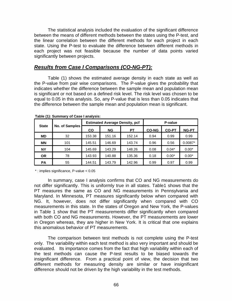
66

The statistical analysis included the evaluation of the significant difference between the means of different methods between the states using the P-test, and the linear correlation between the different methods for each project in each state. Using the P-test to evaluate the difference between different methods in each project was not feasible because the number of data points varied significantly between projects. Results from Case I Comparisons (CO-NG-PT):

Table (1) shows the estimated average density in each state as well as the P-value from pair wise comparisons. The P-value gives the probability that indicates whether the difference between the sample mean and population mean is significant or not based on a defined risk level. The risk level was chosen to be equal to 0.05 in this analysis. So, any P-value that is less than 0.05 indicates that the difference between the sample mean and population mean is significant.

In summary, case I analysis confirms that CO and NG measurements do not differ significantly. This is uniformly true in all states. Table1 shows that the PT measures the same as CO and NG measurements in Pennsylvania and Maryland. In Minnesota, PT measures significantly below when compared with NG. It, however, does not differ significantly when compared with CO measurements in this state. In the states of Oregon and New York, the P-values in Table 1 show that the PT measurements differ significantly when compared with both CO and NG measurements. However, the PT measurements are lower in Oregon whereas, they are higher in New York. It is critical that one explains this anomalous behavior of PT measurements.

The comparison between test methods is not complete using the P-test only. The variability within each test method is also very important and should be evaluated. Its importance comes from the fact that high variability within each of the test methods can cause the P-test results to be biased towards the insignificant difference. From a practical point of view, the decision that two different methods for measuring density are similar or have insignificant difference should not be driven by the high variability in the test methods.

Table (1): Summary of Case I analysis:

CO NG PT CO-NG CO-PT NG-PTMD 32 153.38 151.16 152.14 0.94 0.99 0.99

MN 101 145.51 146.69 143.74 0.96 0.56 0.0087*

NY 104 145.69 143.29 148.26 0.08 0.04* 0.00*

OR 78 143.93 140.88 135.36 0.18 0.00* 0.00*

PA 55 144.51 143.79 142.96 0.99 0.97 0.99

* : implies significance, P-value < 0.05

State No. of SamplesEstimated Average Density, pcf P-value

67

Figure 1 shows the average densities for all states using all methods.

This figure is given for comparison proposes among the states and cannot be used to compare different test methods since each point represents an average of all projects. The data variability for Case I is investigated using the Boxplots. These plots give clear idea and wide range of information about the variability of the density measurements. All illustration of the notation and symbols used in the Boxplots is shown in Figure 2. Figure 3 indicates that the variability of PT measurements are higher than that of CO or NG measurements. Figure 4 shows that the variability in the state of New York is higher than the variability in the other states. For the CO measurements, NY has the highest variability among the other states (Figure 5). New York, Minnesota, and Maryland showed high variability in both the NG and PT density measurements as can be seen in Figures 6 and 7.

Table 2 shows the correlation coefficient, R2, while Table 3 lists and the corresponding linear equation for case I analysis. The R2 is an indication of the variability and scattering of the measurements about their mean. So the R2 cannot be used directly to test the hypothesis of the equality of the population mean and sample mean. If the value of R2 is reasonably high then the corresponding linear equation can be used in calculating the actual density. It can be seen that R2 for CO-NG is higher than that for CO-PT in the majority of the projects. This can be attributed to the high variability in PT compared with NG as shown in the Boxplots presented earlier.

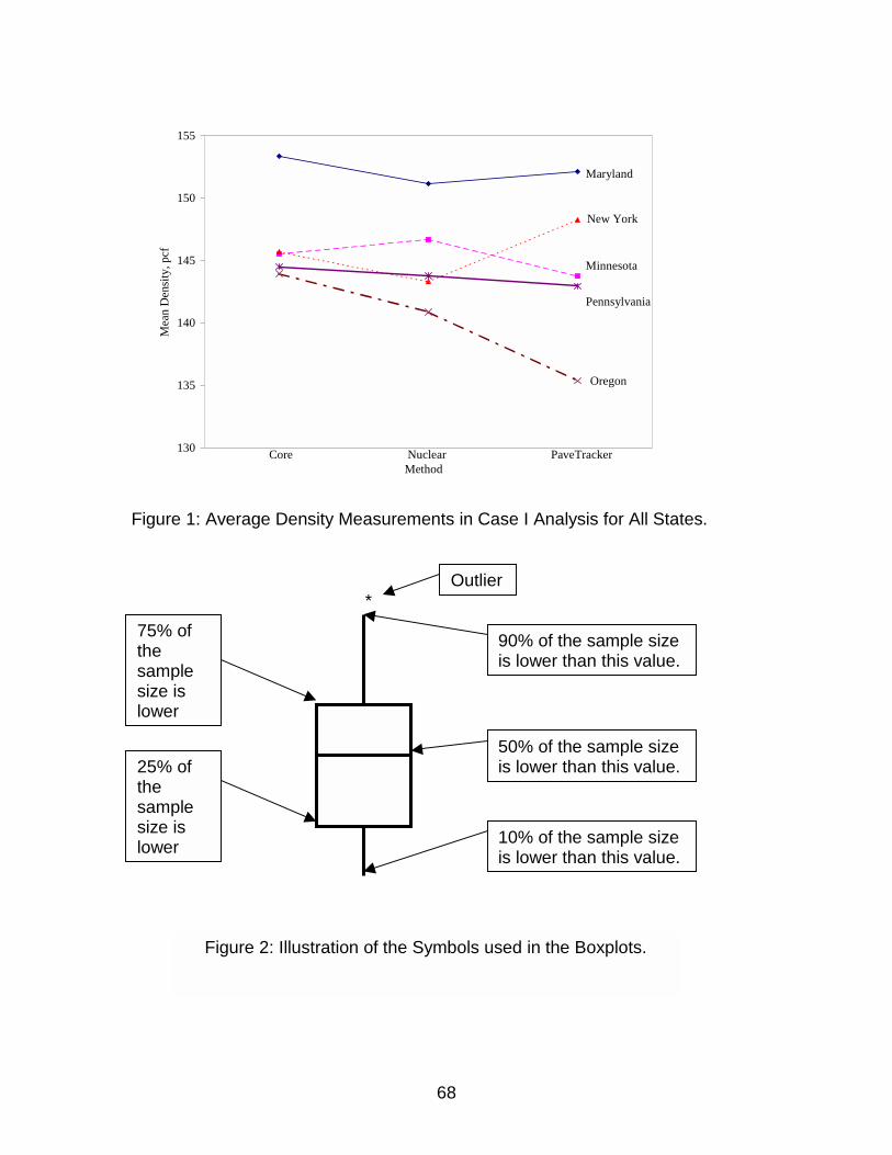
68

Figure 1: Average Density Measurements in Case I Analysis for All States.

Outlier

90% of the sample size is lower than this value.

10% of the sample size is lower than this value.

75% of the sample size is lower

25% of the sample size is lower

50% of the sample size is lower than this value.

Figure 2: Illustration of the Symbols used in the Boxplots.

130

135

140

145

150

155

Method

Mea

n D

ensi

ty, p

cf

Core Nuclear PaveTracker

Maryland

Minnesota

Pennsylvania

Oregon

New York

*

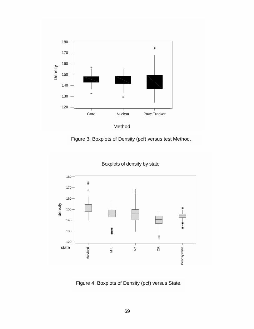
69

Core Nuclear Pave Tracker

120

130

140

150

160

170

180

Den

sity

Figure 3: Boxplots of Density (pcf) versus test Method.

Method

Pen

nsyl

vani

a

OR

NY

Min

.

Mar

ylan

d

180

170

160

150

140

130

120

state

dens

ity

Boxplots of density by state

Figure 4: Boxplots of Density (pcf) versus State.

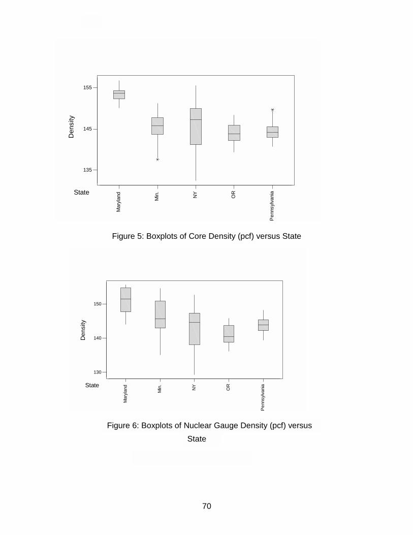
Figure 5: Boxplots of Core Density (pcf) versus State

Mar

ylan

d

Min

.

NY

OR

Pen

nsyl

vani

a

135

145

155

State

Den

sity

Boxplots of Core by State

Mar

ylan

d

Min

.

NY

OR

Pen

nsyl

vani

a

130

140

150

State

Den

sity

Boxplots of Nuclear by State

Figure 6: Boxplots of Nuclear Gauge Density (pcf) versus

70

State

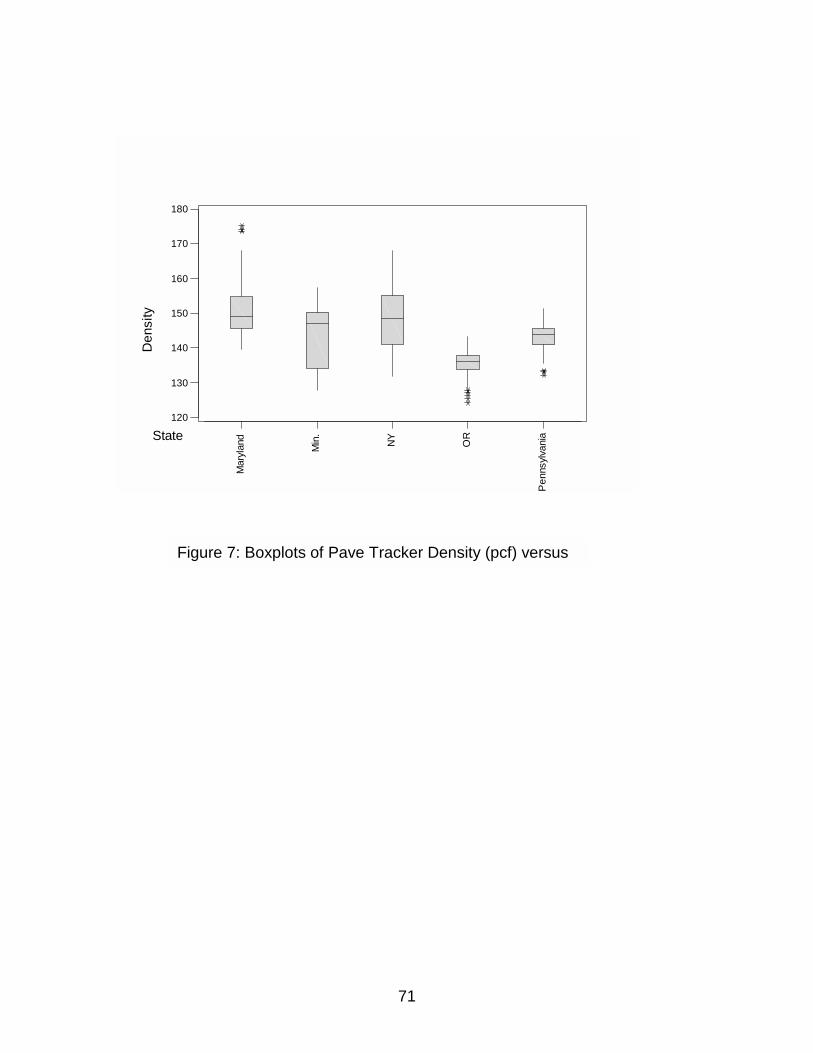
Mar

ylan

d

Min

.

NY

OR

Pen

nsyl

vani

a

120

130

140

150

160

170

180

State

Den

sity

Boxplots of Pave Tracker by State

Figure 7: Boxplots of Pave Tracker Density (pcf) versus

71

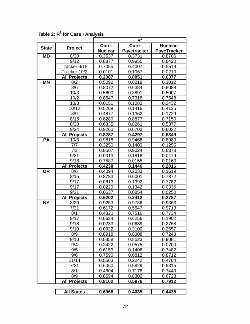
72

Table 2: R2 for Case I Analysis

Core- Core- Nuclear-Nuclear Pavetracker PaveTracker

MD 8/30 0.3537 0.3731 0.87069/12 0.8877 0.9955 0.8420

Tracker 9/15 0.7055 0.4007 0.5519Tracker 10/2 0.0101 0.1067 0.0210All Projects 0.2007 0.0051 0.0377

MN 8/2 0.5092 0.0219 0.10128/6 0.8072 0.6384 0.808810/3 0.5600 0.3891 0.500710/2 0.8547 0.7318 0.754810/3 0.0151 0.1083 0.3432

10/12 0.5268 0.1416 0.41358/9 0.4877 0.1362 0.17298/15 0.8280 0.8877 0.71508/30 0.6335 0.8261 0.53779/24 0.9260 0.6703 0.6022

All Projects 0.8287 0.4297 0.5349PA 10/3 0.9618 0.9468 0.8989

7/7 0.3250 0.1403 0.12557/2 0.8507 0.9024 0.6378

9/21 0.0013 0.1818 0.04799/18 0.7587 0.0155 0.0160

All Projects 0.4238 0.1446 0.2016OR 8/6 0.4094 0.2033 0.1619

8/15 0.8783 0.6001 0.78729/17 0.0813 0.1392 0.77829/17 0.0229 0.1342 0.03369/21 0.0637 0.0854 0.0250

All Projects 0.6202 0.2412 0.2787NY 8/20 0.9253 0.9788 0.9363

7/31 0.6172 0.5547 0.97138/1 0.4820 0.7516 0.77349/17 0.0624 0.6256 0.19029/18 0.0233 0.0689 0.27689/19 0.0922 0.3100 0.26578/9 0.8918 0.8308 0.72439/10 0.8858 0.8523 0.90819/4 0.2422 0.0575 0.07009/5 0.6159 0.1406 0.74829/6 0.7590 0.6812 0.8712

11/14 0.5503 0.2242 0.47047/31 0.6060 0.5829 0.93158/1 0.4804 0.7178 0.74438/9 0.8694 0.8302 0.6723

All Projects 0.8102 0.5976 0.7912

All States 0.6968 0.4035 0.4435

R2

State Project

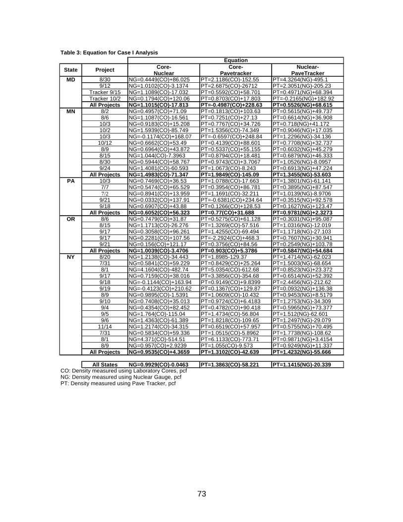
73

Table 3: Equation for Case I Analysis

Core- Core- Nuclear-Nuclear Pavetracker PaveTracker

MD 8/30 NG=0.4449(CO)+86.025 PT=2.1186(CO)-152.55 PT=4.3264(NG)-495.19/12 NG=1.0102(CO)-3.1374 PT=2.6875(CO)-26712 PT=2.3051(NG)-205.23

Tracker 9/15 NG=1.1089(CO)-17.032 PT=0.5592(CO)+58.701 PT=0.4971(NG)+68.394Tracker 10/2 NG=0.1794(CO)+120.06 PT=0.8703(CO)+17.803 PT=-0.2165(NG)+182.92All Projects NG=1.1015(CO)-17.813 PT=-0.4987(CO)+228.63 PT=0.5526(NG)+68.615

MN 8/2 NG=0.4957(CO)+71.09 PT=0.1813(CO)+103.63 PT=0.5615(NG)+49.7378/6 NG=1.1087(CO)-16.561 PT=0.7251(CO)+27.13 PT=0.6614(NG)+36.90810/3 NG=0.9183(CO)+15.208 PT=0.7767(CO)+34.726 PT=0.718(NG)+41.17210/2 NG=1.5939(CO)-85.749 PT=1.5356(CO)-74.349 PT=0.9046(NG)+17.03510/3 NG=-0.1174(CO)+168.07 PT=-0.6597(CO)+248.84 PT=1.2296(NG)-34.136

10/12 NG=0.6662(CO)+53.49 PT=0.4139(CO)+88.601 PT=0.7708(NG)+32.7378/9 NG=0.6964(CO)+43.872 PT=0.5337(CO)+55.155 PT=0.6032(NG)+45.2798/15 NG=1.044(CO)-7.3963 PT=0.8794(CO)+18.481 PT=0.6879(NG)+46.3338/30 NG=0.5944(CO)+58.767 PT=0.9743(CO)+3.7067 PT=1.0526(NG)-8.09579/24 NG=1.4081(CO)-60.593 PT=1.0673(CO)-8.243 PT=0.6913(NG)+47.224

All Projects NG=1.4983(CO)-71.347 PT=1.9849(CO)-145.09 PT=1.3455(NG)-53.603PA 10/3 NG=0.7469(CO)+36.53 PT=1.0788(CO)-17.663 PT=1.3801(NG)-61.141

7/7 NG=0.5474(CO)+65.529 PT=0.3954(CO)+86.781 PT=0.3895(NG)+87.5477/2 NG=0.8941(CO)+13.959 PT=1.1691(CO)-32.211 PT=1.0139(NG)-8.9706

9/21 NG=0.0332(CO)+137.91 PT=-0.6381(CO)+234.64 PT=0.3515(NG)+92.5789/18 NG=0.6907(CO)+43.88 PT=0.1266(CO)+128.53 PT=0.1627(NG)+123.47

All Projects NG=0.6052(CO)+56.323 PT=0.77(CO)+31.688 PT=0.9781(NG)+2.3273OR 8/6 NG=0.7479(CO)+31.87 PT=0.5275(CO)+61.128 PT=0.3031(NG)+95.087

8/15 NG=1.1713(CO)-26.276 PT=1.3269(CO)-57.516 PT=1.0316(NG)-12.0199/17 NG=0.3058(CO)+96.261 PT=1.4255(CO)-69.494 PT=1.1718(NG)-27.1039/17 NG=0.2281(CO)+107.56 PT=-2.2924(CO)+468.3 PT=0.7607(NG)+30.9419/21 NG=0.156(CO)+121.17 PT=0.3756(CO)+84.56 PT=0.2549(NG)+103.78

All Projects NG=1.0039(CO)-3.4706 PT=0.903(CO)+5.3786 PT=0.5847(NG)+54.684NY 8/20 NG=1.2138(CO)-34.443 PT=1.8985-129.37 PT=1.4714(NG)-62.023

7/31 NG=0.5841(CO)+59.229 PT=0.8429(CO)+25.264 PT=1.5003(NG)-68.6548/1 NG=4.1604(CO)-482.74 PT=5.0354(CO)-612.68 PT=0.8523(NG)+23.3729/17 NG=0.7159(CO)+38.016 PT=3.3856(CO)-354.68 PT=0.6514(NG)+52.3929/18 NG=-0.1144(CO)+163.94 PT=0.9149(CO)+9.8399 PT=2.4456(NG)-212.629/19 NG=-0.4123(CO)+210.62 PT=0.1367(CO)+129.87 PT=0.0932(NG)+136.388/9 NG=0.9895(CO)-1.5391 PT=1.0609(CO)-10.432 PT=0.9453(NG)+8.51799/10 NG=0.7408(CO)+35.013 PT=0.9724(CO)+6.4183 PT=1.2753(NG)-34.3099/4 NG=0.4354(CO)+82.452 PT=0.4782(CO)+90.418 PT=0.5965(NG)+73.3779/5 NG=1.764(CO)-115.04 PT=1.4734(CO)-56.804 PT=1.512(NG)-62.6019/6 NG=1.4363(CO)-61.389 PT=1.8218(CO)-109.65 PT=1.2497(NG)-29.079

11/14 NG=1.2174(CO)-34.315 PT=0.6519(CO)+57.957 PT=0.5755(NG)+70.4957/31 NG=0.5834(CO)+59.336 PT=1.0515(CO)-5.8962 PT=1.7738(NG)-108.628/1 NG=4.371(CO)-514.51 PT=6.1133(CO)-773.71 PT=0.9871(NG)+3.41548/9 NG=0.957(CO)+2.9239 PT=1.055(CO)-9.573 PT=0.9249(NG)+11.337

All Projects NG=0.9535(CO)+4.3659 PT=1.3102(CO)-42.639 PT=1.4232(NG)-55.666

All States NG=0.9929(CO)-0.0463 PT=1.3863(CO)-58.221 PT=1.1415(NG)-20.339CO: Density measured using Laboratory Cores, pcfNG: Density measured using Nuclear Gauge, pcfPT: Density measured using Pave Tracker, pcf

EquationState Project

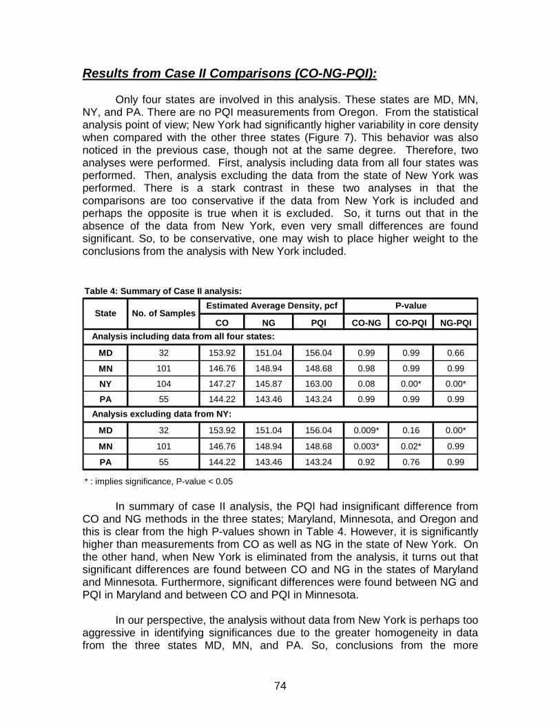
74

Results from Case II Comparisons (CO-NG-PQI):

Only four states are involved in this analysis. These states are MD, MN, NY, and PA. There are no PQI measurements from Oregon. From the statistical analysis point of view; New York had significantly higher variability in core density when compared with the other three states (Figure 7). This behavior was also noticed in the previous case, though not at the same degree. Therefore, two analyses were performed. First, analysis including data from all four states was performed. Then, analysis excluding the data from the state of New York was performed. There is a stark contrast in these two analyses in that the comparisons are too conservative if the data from New York is included and perhaps the opposite is true when it is excluded. So, it turns out that in the absence of the data from New York, even very small differences are found significant. So, to be conservative, one may wish to place higher weight to the conclusions from the analysis with New York included.

In summary of case II analysis, the PQI had insignificant difference from

CO and NG methods in the three states; Maryland, Minnesota, and Oregon and this is clear from the high P-values shown in Table 4. However, it is significantly higher than measurements from CO as well as NG in the state of New York. On the other hand, when New York is eliminated from the analysis, it turns out that significant differences are found between CO and NG in the states of Maryland and Minnesota. Furthermore, significant differences were found between NG and PQI in Maryland and between CO and PQI in Minnesota.

In our perspective, the analysis without data from New York is perhaps too aggressive in identifying significances due to the greater homogeneity in data from the three states MD, MN, and PA. So, conclusions from the more

Table 4: Summary of Case II analysis:

CO NG PQI CO-NG CO-PQI NG-PQI

MD 32 153.92 151.04 156.04 0.99 0.99 0.66

MN 101 146.76 148.94 148.68 0.98 0.99 0.99

NY 104 147.27 145.87 163.00 0.08 0.00* 0.00*

PA 55 144.22 143.46 143.24 0.99 0.99 0.99

MD 32 153.92 151.04 156.04 0.009* 0.16 0.00*

MN 101 146.76 148.94 148.68 0.003* 0.02* 0.99

PA 55 144.22 143.46 143.24 0.92 0.76 0.99

* : implies significance, P-value < 0.05

Analysis excluding data from NY:

Analysis including data from all four states:

State No. of SamplesEstimated Average Density, pcf P-value

75

conservative analysis with data from NY included would be perhaps more desirable, in which case, the only differences identified would be from the state of New York itself. Other differences turn out to be insignificant. As shown in Figures 9 and 10, PQI has the highest variability compared with the other methods, and the highest PQI variability is in NY State. Figure 11 shows the average density for all states. This figure is given for comparison purposes among the different states and cannot be used to compare different methods.

Table 5 shows the coefficient, of determination R2, and Table 6 lists the corresponding linear equation for case II analysis. Again, the linear equation corresponding to a reasonably high value of R2 can be used in calculating the actual density. Considering Table 7, it seems that the R2 values for CO-NG, CO-PQI, and NG-PQI do not differ significantly in each of the four states. As shown in Table 6, R2 for the CO-PQI data was less than that for NG-CO data in most cases.

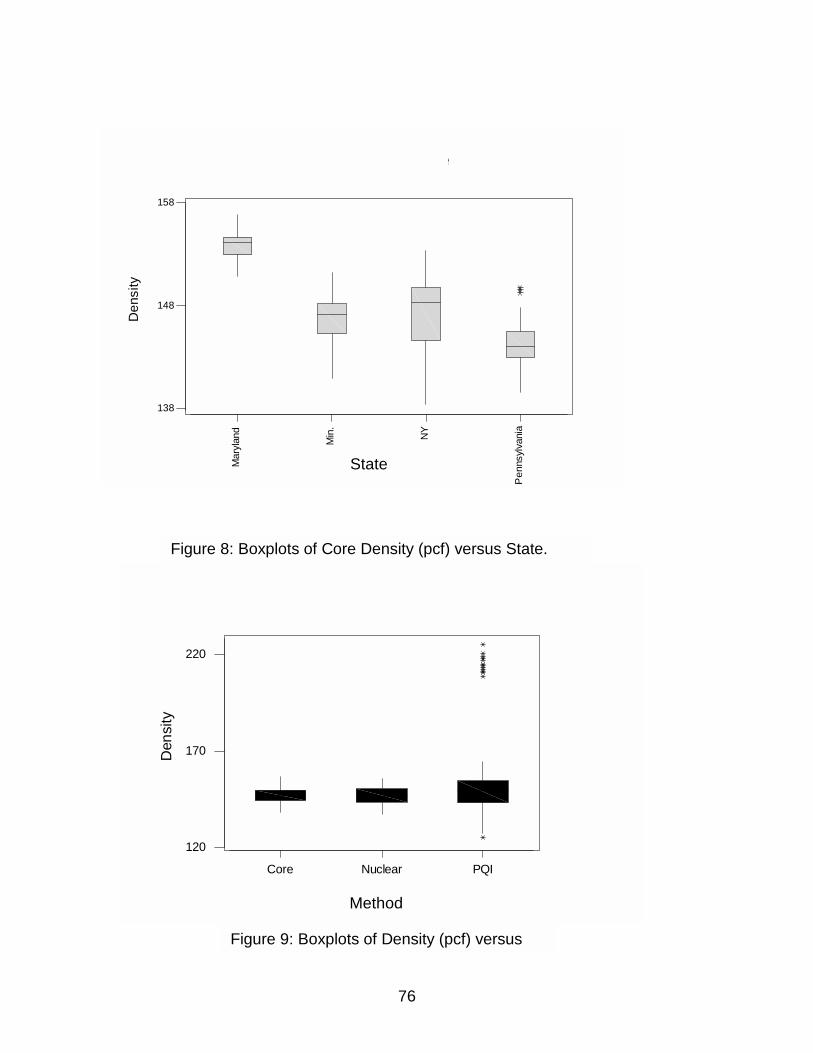
Core Nuclear PQI

120

170

220

Den

sity

Method

Mar

ylan

d

Min

.

NY

Pen

nsyl

vani

a

138

148

158

State

Den

sity

Boxplots of Core by State

State

Figure 8: Boxplots of Core Density (pcf) versus State.

Figure 9: Boxplots of Density (pcf) versus

76

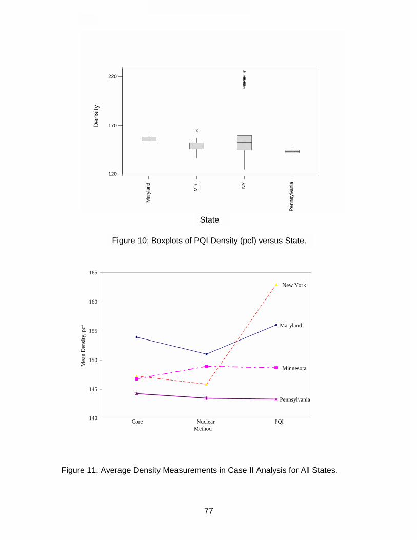
Figur

77

e 11: Average Density Measurements in Case II Analysis for All States.

Figure 10: Boxplots of Nuclear Gauge Density (pcf) versus State

Mar

ylan

d

Min

.

NY

Pen

nsyl

vani

a

120

170

220

State

Den

sity

Boxplots of PQI by State

State

Figure 10: Boxplots of PQI Density (pcf) versus State.

140

145

150

155

160

165

Method

Mea

n D

ensi

ty, p

cf

Core Nuclear PQI

Maryland

Minnesota

Pennsylvania

New York

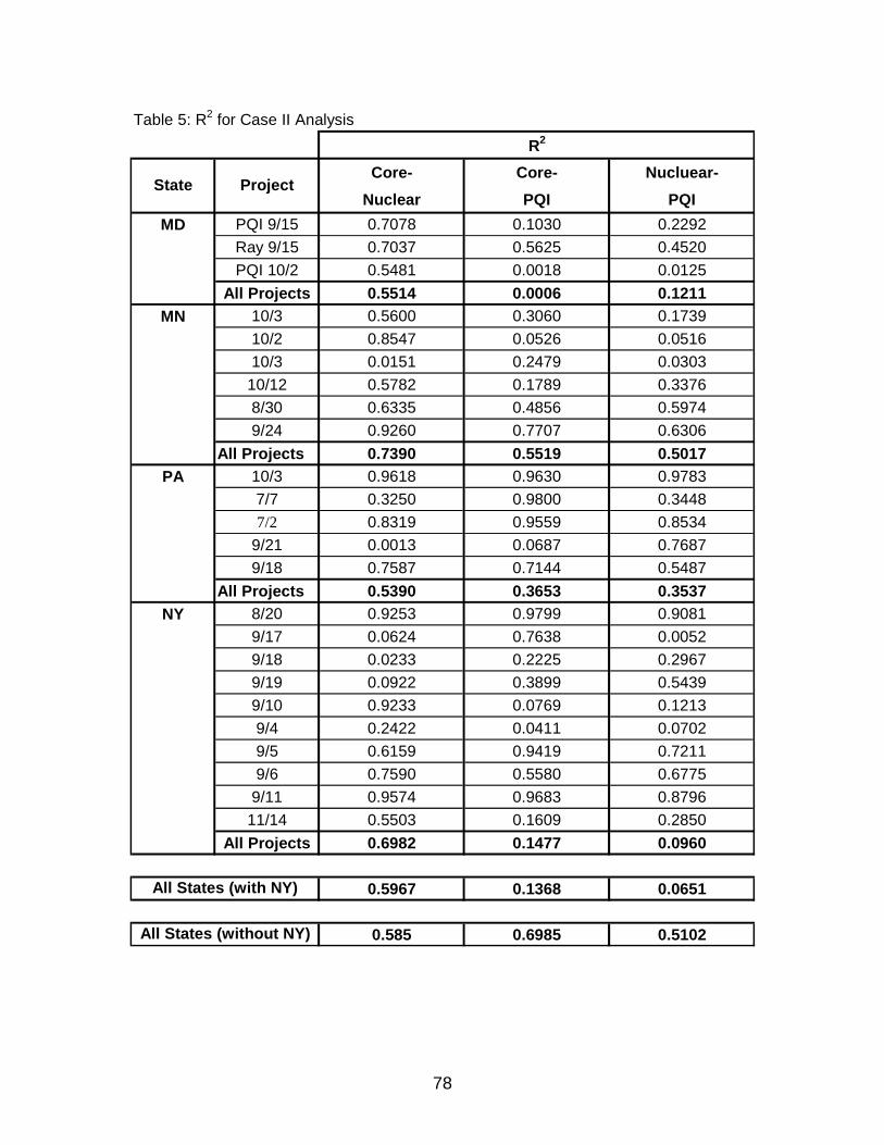
78

Table 5: R2 for Case II Analysis

Core- Core- Nucluear-Nuclear PQI PQI

MD PQI 9/15 0.7078 0.1030 0.2292Ray 9/15 0.7037 0.5625 0.4520PQI 10/2 0.5481 0.0018 0.0125

All Projects 0.5514 0.0006 0.1211MN 10/3 0.5600 0.3060 0.1739

10/2 0.8547 0.0526 0.051610/3 0.0151 0.2479 0.030310/12 0.5782 0.1789 0.33768/30 0.6335 0.4856 0.59749/24 0.9260 0.7707 0.6306

All Projects 0.7390 0.5519 0.5017PA 10/3 0.9618 0.9630 0.9783

7/7 0.3250 0.9800 0.34487/2 0.8319 0.9559 0.8534

9/21 0.0013 0.0687 0.76879/18 0.7587 0.7144 0.5487

All Projects 0.5390 0.3653 0.3537NY 8/20 0.9253 0.9799 0.9081

9/17 0.0624 0.7638 0.00529/18 0.0233 0.2225 0.29679/19 0.0922 0.3899 0.54399/10 0.9233 0.0769 0.12139/4 0.2422 0.0411 0.07029/5 0.6159 0.9419 0.72119/6 0.7590 0.5580 0.6775

9/11 0.9574 0.9683 0.879611/14 0.5503 0.1609 0.2850

All Projects 0.6982 0.1477 0.0960

0.5967 0.1368 0.0651

0.585 0.6985 0.5102

All States (with NY)

All States (without NY)

State Project

R2

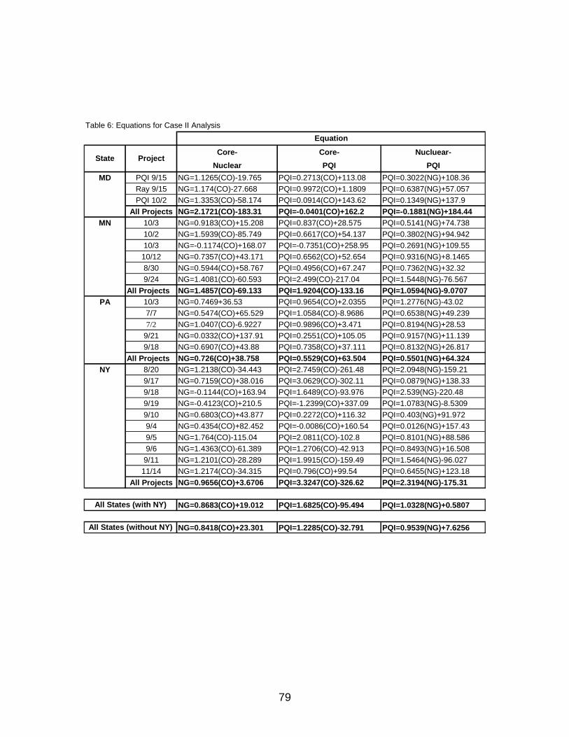
79

Table 6: Equations for Case II Analysis

Core- Core- Nucluear-Nuclear PQI PQI

MD PQI 9/15 NG=1.1265(CO)-19.765 PQI=0.2713(CO)+113.08 PQI=0.3022(NG)+108.36Ray 9/15 NG=1.174(CO)-27.668 PQI=0.9972(CO)+1.1809 PQI=0.6387(NG)+57.057PQI 10/2 NG=1.3353(CO)-58.174 PQI=0.0914(CO)+143.62 PQI=0.1349(NG)+137.9

All Projects NG=2.1721(CO)-183.31 PQI=-0.0401(CO)+162.2 PQI=-0.1881(NG)+184.44MN 10/3 NG=0.9183(CO)+15.208 PQI=0.837(CO)+28.575 PQI=0.5141(NG)+74.738

10/2 NG=1.5939(CO)-85.749 PQI=0.6617(CO)+54.137 PQI=0.3802(NG)+94.94210/3 NG=-0.1174(CO)+168.07 PQI=-0.7351(CO)+258.95 PQI=0.2691(NG)+109.5510/12 NG=0.7357(CO)+43.171 PQI=0.6562(CO)+52.654 PQI=0.9316(NG)+8.14658/30 NG=0.5944(CO)+58.767 PQI=0.4956(CO)+67.247 PQI=0.7362(NG)+32.329/24 NG=1.4081(CO)-60.593 PQI=2.499(CO)-217.04 PQI=1.5448(NG)-76.567

All Projects NG=1.4857(CO)-69.133 PQI=1.9204(CO)-133.16 PQI=1.0594(NG)-9.0707PA 10/3 NG=0.7469+36.53 PQI=0.9654(CO)+2.0355 PQI=1.2776(NG)-43.02

7/7 NG=0.5474(CO)+65.529 PQI=1.0584(CO)-8.9686 PQI=0.6538(NG)+49.2397/2 NG=1.0407(CO)-6.9227 PQI=0.9896(CO)+3.471 PQI=0.8194(NG)+28.53

9/21 NG=0.0332(CO)+137.91 PQI=0.2551(CO)+105.05 PQI=0.9157(NG)+11.1399/18 NG=0.6907(CO)+43.88 PQI=0.7358(CO)+37.111 PQI=0.8132(NG)+26.817

All Projects NG=0.726(CO)+38.758 PQI=0.5529(CO)+63.504 PQI=0.5501(NG)+64.324NY 8/20 NG=1.2138(CO)-34.443 PQI=2.7459(CO)-261.48 PQI=2.0948(NG)-159.21

9/17 NG=0.7159(CO)+38.016 PQI=3.0629(CO)-302.11 PQI=0.0879(NG)+138.339/18 NG=-0.1144(CO)+163.94 PQI=1.6489(CO)-93.976 PQI=2.539(NG)-220.489/19 NG=-0.4123(CO)+210.5 PQI=-1.2399(CO)+337.09 PQI=1.0783(NG)-8.53099/10 NG=0.6803(CO)+43.877 PQI=0.2272(CO)+116.32 PQI=0.403(NG)+91.9729/4 NG=0.4354(CO)+82.452 PQI=-0.0086(CO)+160.54 PQI=0.0126(NG)+157.439/5 NG=1.764(CO)-115.04 PQI=2.0811(CO)-102.8 PQI=0.8101(NG)+88.5869/6 NG=1.4363(CO)-61.389 PQI=1.2706(CO)-42.913 PQI=0.8493(NG)+16.508

9/11 NG=1.2101(CO)-28.289 PQI=1.9915(CO)-159.49 PQI=1.5464(NG)-96.02711/14 NG=1.2174(CO)-34.315 PQI=0.796(CO)+99.54 PQI=0.6455(NG)+123.18

All Projects NG=0.9656(CO)+3.6706 PQI=3.3247(CO)-326.62 PQI=2.3194(NG)-175.31

NG=0.8683(CO)+19.012 PQI=1.6825(CO)-95.494 PQI=1.0328(NG)+0.5807

NG=0.8418(CO)+23.301 PQI=1.2285(CO)-32.791 PQI=0.9539(NG)+7.6256

All States (with NY)

All States (without NY)

Equation

State Project

80

Summary of Findings: The following points summarize the main findings from this study:

• Comparisons between PQI and PaveTracker measurements could not been established due to the lack of the appropriate data. So comparisons were limited to Core-Nuclear Gauge-Pave Tracker or Core-Nuclear Gauge-PQI only.

• The PaveTracker is significantly different from the cores in two of the five states, and it is significantly different from Nuclear Gauge in three of the five states.

• The Pavetracker has higher variability than the core measurements and Nuclear Gauge. This high variability affects the results of the P-test. When the variability within the test methods increases, the difference between the test methods is skewed to be insignificant. From practical point of view, the conclusion of two methods being insignificantly different should not be caused by the high variability.

• The Nuclear Gauge method has higher correlation with core measurements than PaveTracker with core measurements in most of the projects.

• The PaveTracker measurements compare favorably with both core and Nuclear Gauge measurements in the states of Maryland and Pennsylvania. They are significantly higher in New York and significantly lower in Oregon when compared with both core and Nuclear Gauge measurements.

• In Minnesota, PaveTracker measurements are significantly lower when compared with Nuclear Gauge measurements only.

• The PQI is significantly different from the cores in one of the four states, and it is significantly different from Nuclear Gauge in one of the four states.

• The PQI has higher variability than the core measurements and Nuclear Gauge.

• The Nuclear Gauge method has higher correlation with core measurements than PQI with core measurements in most of the projects.

• The state of Pennsylvania stands out in the whole analysis in the sense that both PaveTracker as well as PQI measurements compare well with core and Nuclear Gauge measurements.

• New York also stands out in a rather different way. In New York, all measurements show greater variability with PQI measurements showing unacceptably high variability in this state. The enclosed Boxplots show this behavior very clearly.