Embed Size (px)
Citation preview
University of Southern Queensland Faculty of Engineering and Surveying
Evaluation of Ashtech ProMark2 Survey System
A dissertation submitted by
Neil Geoffrey Shaw
In fulfillment of the requirements of
Courses ENG4111 and ENG4112 Research Project
Towards the degree of Bachelor of Spatial Science (Surveying)
October 2006
ABSTRACT
The use of GPS receivers in surveying has become widespread. The limiting
factor for many firms remains the relatively high cost of the equipment. This
project evaluates the performance of the Ashtech ProMark2 survey system.
The Ashtech system comprises two single frequency (L1) receivers and a
suite of software for processing, mission planning and file conversions. At
the time of purchase the system was approximately 1/6th of the price of a
pair of RTK receivers. The Ashtech ProMark2, however the Ashtech system
provides post processed results only (no real time capabilities).
The objective of the project is to establish what level of accuracy is
achievable using the Ashtech ProMark2. Also to determine the effect of
changes in baseline length, number of available satellites, dilution of
precision and observation duration. Some recommendations as to
appropriate observation durations depending on existing conditions are also
made.
i

University of Southern Queensland
Faculty of Engineering and Surveying
ENG4111 & ENG4112 Research Project
Limitations of use
The Council of the University of Southern Queensland, its Faculty of
Engineering and Surveying, and the staff of the University of Southern
Queensland, do not accept any responsibility for the truth, accuracy or
completeness of material contained within or associated with this
dissertation.
Persons using all or any part of this material do so at their own risk, and not
at the risk of the Council of the University of Southern Queensland, its
Faculty of Engineering and Surveying or the staff of the University of
Southern Queensland.
This dissertation reports an educational exercise and has no purpose or
validity beyond this exercise. The sole purpose of the course pair entitled
"Research Project" is to contribute to the overall education within the
student’s chosen degree program. This document, the associated hardware,
software, drawings, and other material set out in the associated appendices
should not be used for any other purpose: if they are so used, it is entirely at
the risk of the user.
Prof. R Smith Dean Faculty of Engineering and Surveying
ii

Certification
I certify that the ideas, designs and experimental work, results, analysis and
conclusions set out in this dissertation are entirely my own effort, except
where otherwise indicated and acknowledged.
I further certify that the work is original and has not been previously
submitted for assessment in any other course or institution, except where
specifically stated.
Neil Geoffrey Shaw
Student Number: 0011020744
______________________________________ Signature
______________________________________ Date
iii

Acknowledgements Mr. Glenn Campbell from the University of Southern Queensland for his
guidance and assistance in supervising the work undertaken in this project.
Mr. Geoff Shaw for the use of equipment and allowances for time to
complete this project. Also for aiding in the field work component of the
project.
And finally my wife Sharon and sons Ryan and Brody for their
understanding and patience during the course of this project.
iv
Table of Contents Abstract i
Limitations of use ii
Certification iii
Acknowledgements iv
List of figures viii
List of tables ix
Glossary of Terms x
Chapter 1 Introduction 1
1.1 Outline of Study. 1
1.2 Introduction. 1
1.3 The Problem. 4
1.4 Research Objectives. 5
1.5 Conclusion. 6
Chapter 2 Literature Review 7
2.1 Introduction. 7
2.2 Need for evaluation. 7
2.3 GPS Surveying. 8
2.4 Survey Accuracy Regulations. 12
2.5 Recommended Static Surveying Practices. 13
2.6 Validation Methods for GPS Receivers. 15
2.7 Satellite Orbit Period. 17
2.8 Control Mark Accuracy. 18
2.9 Conclusion. 19
Chapter 3 Methodology 21
3.1 Introduction. 21
v
3.2 Expectations. 22
3.3 Reference Marks. 22
3.4 Fieldwork. 22
3.5 Analysis. 23
3.6 Data Analysis. 25
3.7 Conclusion. 25
Chapter 4 Results. 27
4.1 Introduction. 27
4.2 Results compared with Known Coordinates. 27
4.3 Results compared with Adjusted Coordinates. 41
4.4 Effects of observation time. 44
4.5 Effects of baseline length. 45
4.6 Effects of number of available satellites. 47
4.7 Effects of PDOP. 51
4.8 Conclusion. 52
Chapter 5 Conclusion. 53
5.1 Introduction. 53
5.2 Results. 53
5.3 Recommendations. 54
5.4 Limitations. 56
5.5 Further work. 57
5.6 Conclusion. 57
References 59
Appendices 61
Appendix A Project Specification 61
Appendix B Accuracy Standards. 63
Appendix C Locality Map. 70
vi

Appendix D Permanent Survey Mark Sketch Plans. 72
vii
List of figures Figure 1.1 Ashtech ProMark2 surveying system receiver pack. 4
Figure 1.2 Ashtech ProMark2 surveying system set up on tripod. 5
Figure 4.1 Misclose – Observation Time 1km 4 satellites. 34
Figure 4.2 Misclose – Obs. Time 1km 4 SVs expanded scale. 34
Figure 4.3 Misclose – Observation Time1km 8 satellites. 35
Figure 4.4 Misclose – Observation Time 15km 4 satellites. 35
Figure 4.5 Misclose – Observation Time 15km 8 satellites. 36
Figure 4.6 Misclose –Baseline Length 4 satellites 30 minutes. 45
Figure 4.7 Misclose – Baseline Length 6 satellites 60 minutes. 46
Figure 4.8 Misclose – Baseline Length 8 satellites 90 minutes. 46
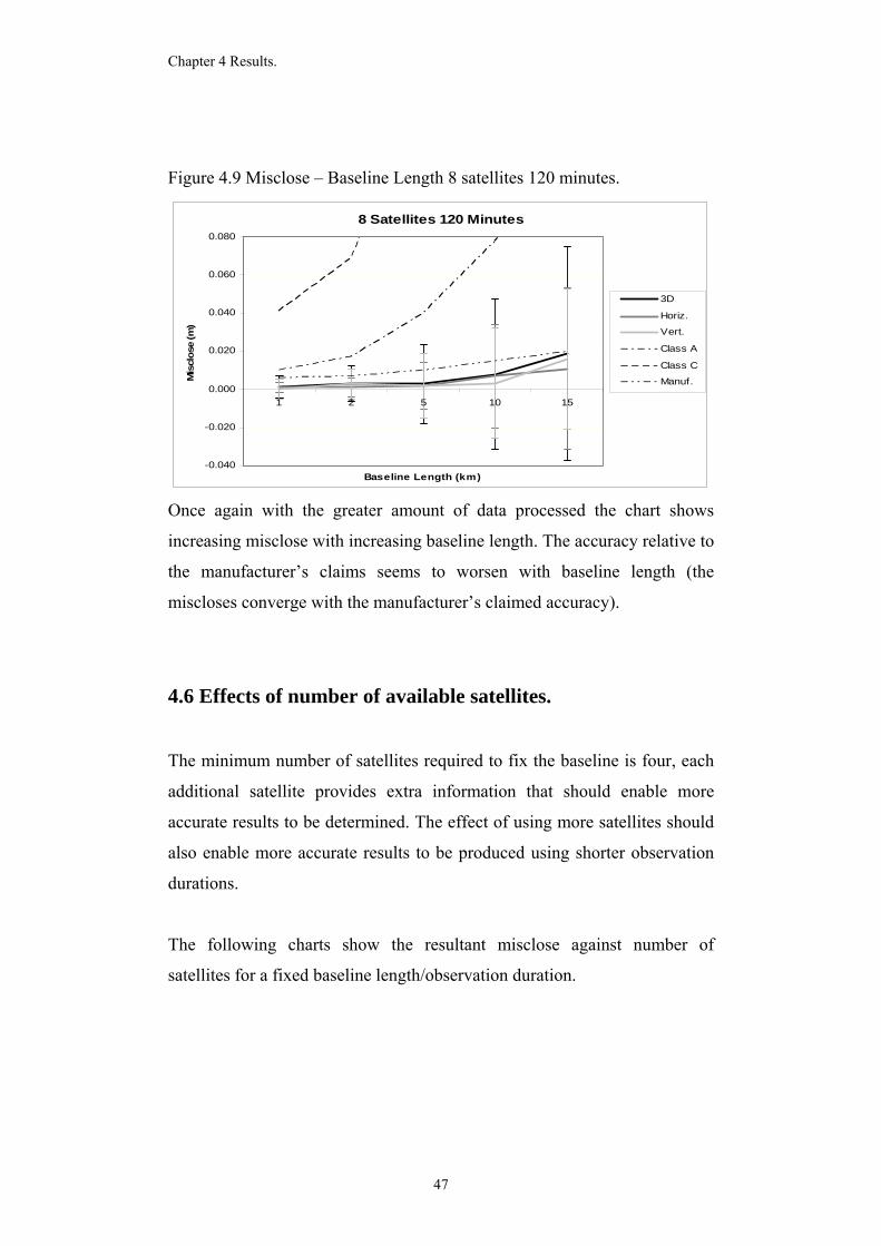
Figure 4.9 Misclose – Baseline Length 8 satellites 120 minutes. 47
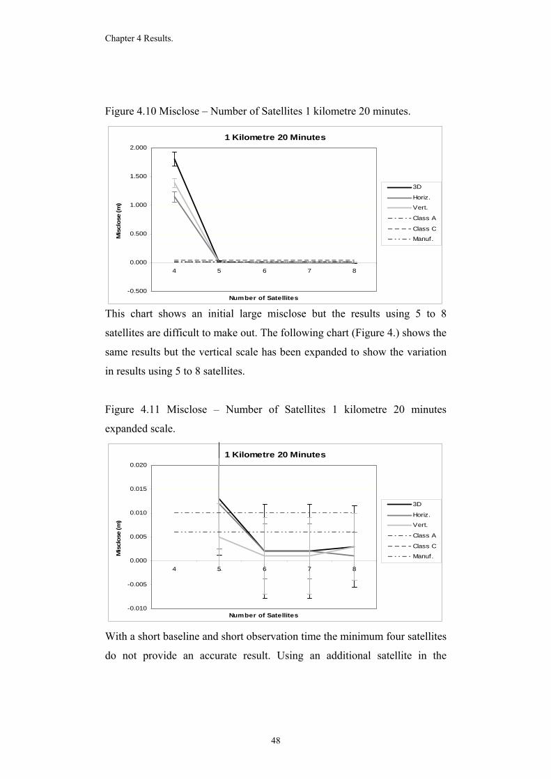
Figure 4.10 Misclose – Number of Satellites 1km 20 minutes. 48
Figure 4.11 Misclose – No. of SVs 1km 20 min expanded scale. 48
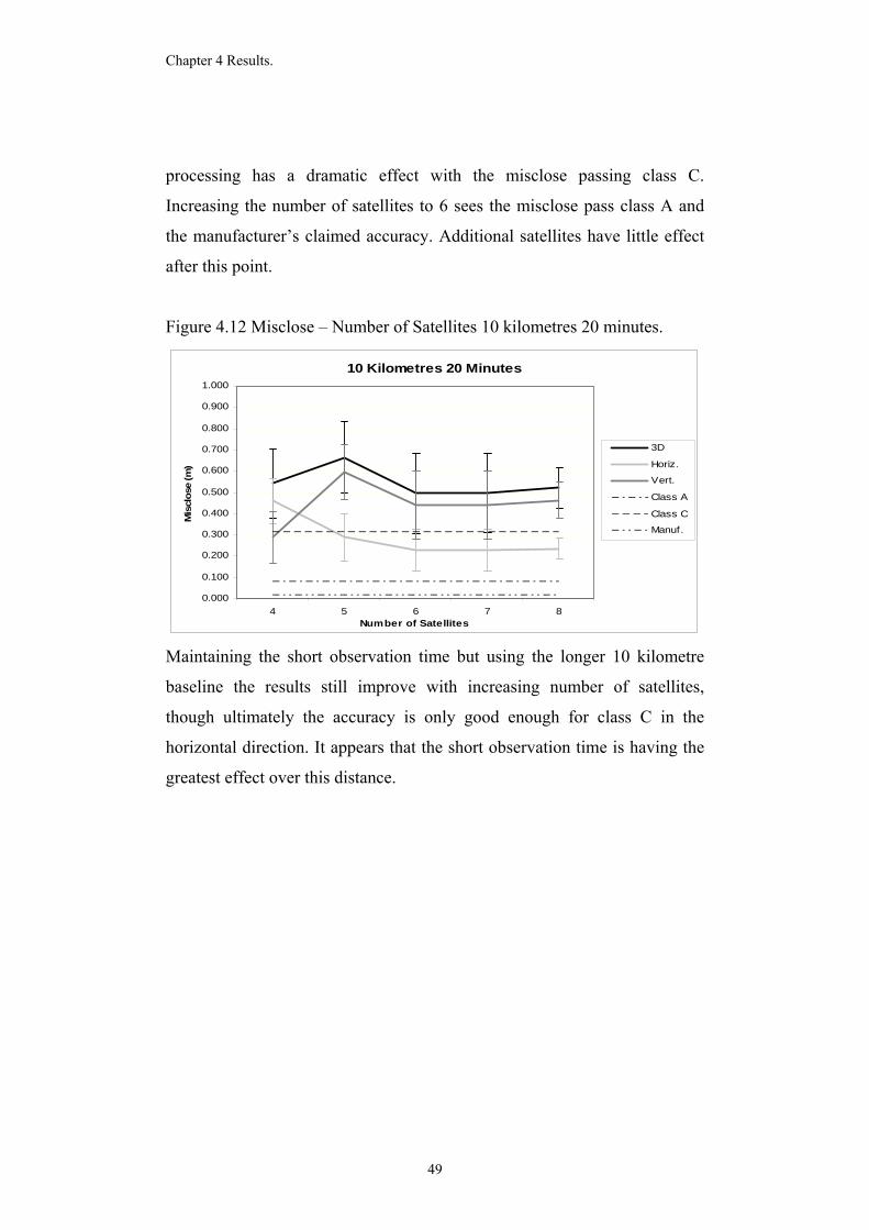
Figure 4.12 Misclose – Number of Satellites 10km 20 minutes. 49
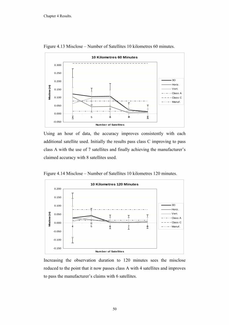
Figure 4.13 Misclose – Number of Satellites 10km 60 minutes. 50
Figure 4.14 Misclose – Number of Satellites 10km 120 minutes. 50
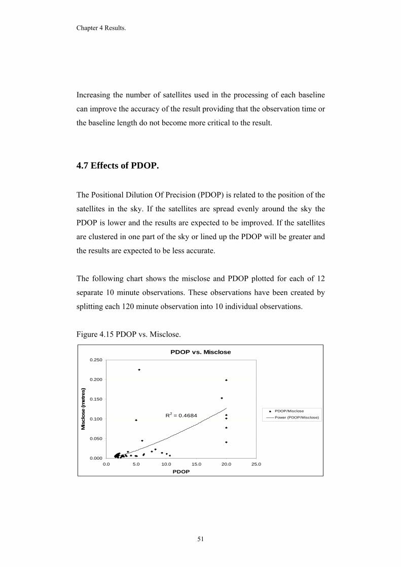
Figure 4.15 PDOP vs. Misclose.. 51
viii
List of tables
Table 2.1 Summary of accuracy standards. 13
Table 2.2 Survey of a class – Highest order relationship. 19
Table 3.1 Vectors to be processed. 24
Table 4.1 Known PSM coordinates. 28
Table 4.2 Observed vectors calculated from known coordinates. 28
Table 4.3 Vectors to be processed. 29
Table 4.4 Sample calculation 1km 4 satellites. 31
Table 4.5 Sample calculation 1km 8 satellites. 32
Table 4.6 Accuracy limits for each baseline. 33
Table 4.7 Minimum observation times using known coordinates. 37
Table 4.8 Loop closure using 8 Satellites. 40
Table 4.9 Adjusted coordinates. 42
Table 4.10 Adjusted vectors. 42
Table 4.11 Minimum observation times using adjusted coordinates. 43
Table 5.1 Minimum observation times. 55
ix
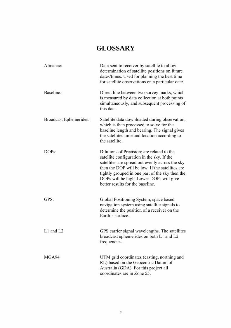
GLOSSARY Almanac: Data sent to receiver by satellite to allow
determination of satellite positions on future dates/times. Used for planning the best time for satellite observations on a particular date.
Baseline: Direct line between two survey marks, which
is measured by data collection at both points simultaneously, and subsequent processing of this data.
Broadcast Ephemerides: Satellite data downloaded during observation,
which is then processed to solve for the baseline length and bearing. The signal gives the satellites time and location according to the satellite.
DOPs: Dilutions of Precision; are related to the
satellite configuration in the sky. If the satellites are spread out evenly across the sky then the DOP will be low. If the satellites are tightly grouped in one part of the sky then the DOPs will be high. Lower DOPs will give better results for the baseline.
GPS: Global Positioning System, space based navigation system using satellite signals to determine the position of a receiver on the Earth’s surface.
L1 and L2 GPS carrier signal wavelengths. The satellites broadcast ephemerides on both L1 and L2 frequencies.
MGA94 UTM grid coordinates (easting, northing and RL) based on the Geocentric Datum of Australia (GDA). For this project all coordinates are in Zone 55.
x
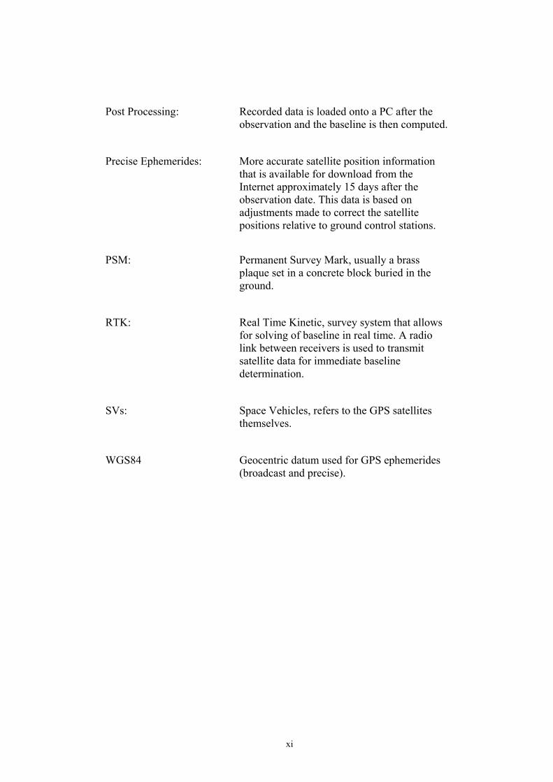
Post Processing: Recorded data is loaded onto a PC after the observation and the baseline is then computed.
Precise Ephemerides: More accurate satellite position information that is available for download from the Internet approximately 15 days after the observation date. This data is based on adjustments made to correct the satellite positions relative to ground control stations.
PSM: Permanent Survey Mark, usually a brass plaque set in a concrete block buried in the ground.
RTK: Real Time Kinetic, survey system that allows for solving of baseline in real time. A radio link between receivers is used to transmit satellite data for immediate baseline determination.
SVs: Space Vehicles, refers to the GPS satellites themselves.
WGS84 Geocentric datum used for GPS ephemerides (broadcast and precise).
xi
Chapter 1 Introduction.
CHAPTER 1
INTRODUCTION
1.1 Outline of Study.
This study aims to evaluate the Static Mode performance of the Ashtech
ProMark 2 GPS survey system (including two receivers, antennae, cables
and software packages). Evaluation will be carried out with respect to
variance in baseline length, number of satellites or space vehicles (SV’s),
dilutions of precision (DOP’s) and observation times. It was hoped that the
evaluation would have used both broadcast and precise ephemeredes for
comparison. The author was unable to process downloaded precise files in
the software (support from the manufacturer was unavailable in time to
include in this report).
1.2 Introduction.
The Global Positioning System is a system of satellites and ground based
monitoring stations designed to enable users to determine their position on
the Earth’s surface. The system was designed and implemented by the US
military for navigation and coordination of military assets.
Many civilian companies have since produced commercially available
navigation and surveying tools. Civilian use of GPS extends to:
- Navigation of ships, aircraft and other vehicles (including satellite
navigation systems available for cars).
1
Chapter 1 Introduction.
- Hand held personal location and navigation devices for use by
campers and hikers.
- Tracking devices to locate company assets such as trucks, ships and
trains. Or security tracking devices to locate stolen vehicles.
- Land surveying to locate specific features on the Earth for the
purposes of mapping, design work, setout for construction etc.
The global positioning system consists of three segments: The space
segment of GPS is a constellation of 24 satellites. The control segment
consists of a control centre and access to overseas command stations and the
user segment includes GPS receivers and associated equipment. (Pace et al.
1995).
GPS survey equipment is capable of making baseline measurements using
static, rapid static, kinematic and real-time kinematic (RTK).
Static surveying is where two or more locations (one receiver at each) are
occupied simultaneously for a length of time to collect data. A minimum of
4 common (to both receiver locations) satellites must be observed at each
site. The coordinate differences between the two points can then be
determined with sufficient accuracy. Observation processing requires the
data to be post-processed (uploaded to computer for software processing to
determine the coordinate differences between the two points).
Rapid Static surveying uses a base station fixed on a known point and a
rover (a separate receiver) attached to a pole such that it can be carried from
point to point. This method requires an initialisation period that measures a
known baseline length for a length of time sufficient to remove most errors
from the solution. This method requires the data to be post-processed.
2
Chapter 1 Introduction.
Kinematic surveying also uses a rover and base station similar to rapid static
(including the requirement for initialisation) but it measures points
approximately every second while the rover is in motion. The data collected
can then be processed to determine the path the rover took. This method
requires the data to be post-processed.
Real Time Kinematic (RTK) surveying is similar to kinematic surveying but
utilises a radio or other communication link between receivers to allow
computer processing for coordinate differences (and hence the rover
location) in real time.
The advantages that GPS based survey systems have over conventional
total-station survey equipment include:
- No requirement for direct line of sight between occupied points.
- Long baselines (many kilometres) can be observed in one
observation.
Disadvantages include:
- The need for an unobstructed ‘view’ of the sky at each occupied
position.
- Many factors can introduce errors into GPS observations such as;
multipath (satellite signals that have been reflected off buildings
etc.) and atmospheric variations.
- Requirement for at least 4 common satellites to be visible at both
locations.
3
Chapter 1 Introduction.
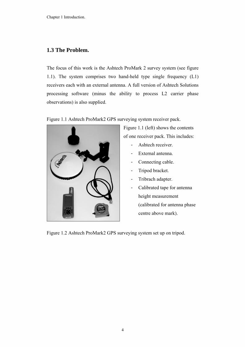
1.3 The Problem.
The focus of this work is the Ashtech ProMark 2 survey system (see figure
1.1). The system comprises two hand-held type single frequency (L1)
receivers each with an external antenna. A full version of Ashtech Solutions
processing software (minus the ability to process L2 carrier phase
observations) is also supplied.
Figure 1.1 Ashtech ProMark2 GPS surveying system receiver pack.
Figure 1.1 (left) shows the contents
of one receiver pack. This includes:
- Ashtech receiver.
- External antenna.
- Connecting cable.
- Tripod bracket.
- Tribrach adapter.
- Calibrated tape for antenna
height measurement
(calibrated for antenna phase
centre above mark).
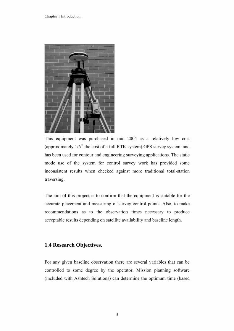
Figure 1.2 Ashtech ProMark2 GPS surveying system set up on tripod.
4
Chapter 1 Introduction.
This equipment was purchased in mid 2004 as a relatively low cost
(approximately 1/6th the cost of a full RTK system) GPS survey system, and
has been used for contour and engineering surveying applications. The static
mode use of the system for control survey work has provided some
inconsistent results when checked against more traditional total-station
traversing.
The aim of this project is to confirm that the equipment is suitable for the
accurate placement and measuring of survey control points. Also, to make
recommendations as to the observation times necessary to produce
acceptable results depending on satellite availability and baseline length.
1.4 Research Objectives.
For any given baseline observation there are several variables that can be
controlled to some degree by the operator. Mission planning software
(included with Ashtech Solutions) can determine the optimum time (based
5
Chapter 1 Introduction.
on satellite availability) at which to perform an observation. The duration of
the observation is infinitely variable and care must be taken that the
observation is long enough to provide sufficient data to process an accurate
result.
This project aims to determine the accuracy possible using the equipment
with variations in the number of satellites, DOP’s, baseline length and
observation duration.
The research methodology is divided into five subparts these being…
1. Research information relevant to the problem.
2. Perform field observations of different length baselines under
controlled conditions.
3. Reduce and analyse the fieldwork for each baseline using varied
combinations of observation times, number of satellites and
DOP’s.
4. Determine recommended minimum observation times depending
on variations in each tested condition.
1.5 Conclusion.
This project aims to confirm the suitability of the Ashtech ProMark 2 survey
system for static mode control survey work and to determine the required
observation times with respect to varying baseline length, number of
available satellites, and the corresponding variations in DOP’s.
6
Chapter 2 Literature Review.
CHAPTER 2
LITERATURE REVIEW
2.1 Introduction.
This chapter will review literature to establish the need for reliably accurate
GPS measurements. This review will describe how survey observations are
made using GPS equipment. This review will identify what regulations are
in place to control the type and condition of survey equipment used, as well
as the accuracy required for survey measurements in Victoria, New South
Wales and Queensland. The review will also determine what recommended
best practices exist for performing static GPS surveys, as well as methods
for evaluating the accuracy of GPS receivers. Finally this review will
establish the accuracy of permanent survey marks available for baseline
measurement in this project.
2.2 Need for evaluation.
Each GPS surveying system exhibits varying characteristics due to the
differences in the hardware and software utilised. There is a need then to test
each different system to ensure that consumers are being offered a
competent surveying tool.
The Federal (USA) Geodetic Control Subcommittee (FGCS) have tested all
GPS surveying instrumentation as it has been released onto the market. The
tests have been carried out using single and dual frequency receivers. No
7
Chapter 2 Literature Review.
other country has systematically tested GPS surveying receivers in this way
(SNAP-UNSW 1999a). This suggests that the Ashtech Promark2 has
already been tested in North America; however the difference in location
can have an effect on equipment performance. Some GPS errors/biases are a
function of geographic location – “how can a test be considered conclusive
if it is carried out in only one location?” (SNAP-UNSW 1999b).
This project is aimed at determining the accuracy achievable using the
Ashtech ProMark2 system. The assumption is made that the FGCS has
already tested the equipment in North America. However local error sources
may be affecting the equipment and therefore the results. The fact that the
equipment has been previously tested in the USA does not provide
conclusive evidence of its performance in southern Australia.
2.3 GPS Surveying.
The Survey Board of Victoria states that GPS is suitable for a broad range
of surveying applications including; cadastral/engineering setout,
topographic mapping, and geodetic control (Survey Board Victoria 2006).
Traditionally, GPS has been used for high precision geodetic survey,
engineering and topographical surveys (via post processing and real time
techniques) (Survey Board Victoria 2006). In reality GPS is just another
surveying tool and as such may be used in conjunction with traditional
methods to provide sufficient information to fix boundaries, marks and
occupation (Survey Board Victoria 2006).
8
Chapter 2 Literature Review.
The Surveyors (Cadastral Survey) Regulations 1995 (for Victoria) state that
a licensed surveyor must:
1. use survey equipment which has been compared to a standard of
measurement in units specified in Part A schedule 6 of the Survey
Coordination (Surveys) Regulations 1992
2. ensure that the process and basis of comparison are adequate to
obtain the accuracy for a cadastral survey under Regulation 6, and
3. retain records of comparisons and make them available to the
Surveyor-General if requested.
The above information suggests that GPS equipment may be used at the
surveyor’s discretion providing that accuracy requirements for the work are
met.
2.3.1 Differential GPS Observations.
The basic GPS positioning technique relies on a distance resection
computation. A receiver on the earth tracks the signals transmitted from
orbiting satellites. Using these signals the range, or distance, to each
satellite is determined (Survey Board Victoria 2006). In order to process
for the baseline between two points a minimum of four satellites must be
observed simultaneously at both receivers.
The locations of the satellites must be known at the instant the satellite
signal is transmitted. Each GPS satellite broadcasts its location in terms
of an ephemeris (the broadcast ephemeris), which is generally accurate to
better than 10 metres (Survey Board Victoria 2006).
9
Chapter 2 Literature Review.
By using two GPS receivers tracking the same satellites simultaneously,
it is possible to remove many systematic errors and improve the relative
position estimates to metre- or millimetre-level (Survey Board Victoria
2006).
GPS surveying equipment is capable of tracking the carrier phase signals.
The GPS L1 and L2 bands have wavelengths of approximately 19 and 24
centimetres respectively (Survey Board Victoria 2006). The Ashtech
ProMark2 system observes the 19cm L1 carrier signal only. Given that
the carrier wavelengths can be tracked to within a few percent of the
wavelength, this means that millimetre-level positioning is possible.
Unfortunately, carrier phase measurements contain a cycle ambiguity
term that must be resolved to obtain accurate results (Survey Board
Victoria 2006). Cycle ambiguity is the unknown number of whole carrier
wavelengths between the satellite and receiver (USACE 2003).
Successful ambiguity resolution is required for baseline formulations.
Generally, in static surveying, ambiguity resolution can be achieved
through long-term averaging and simple geometric calibration principles,
resulting in solutions to a linear equation that produces a resultant
position. Thus 30 minutes or more of observations may be required to
resolve the ambiguities in static surveys (USACE 2003).
10
Chapter 2 Literature Review.
2.3.2 Static Mode Observations.
Static observations are made by occupying two (or more) survey points
with a receiver each. The simultaneous satellite observations can then be
processed to provide coordinate differences in X, Y and Z based in the
WGS84 geocentric ellipsoid (USACE 2003). The coordinate differences
can then be computed as differences in a local coordinate system such as
MGA94.
Static observing sessions can range from 20 minutes to 3 hours in length.
A single epoch of data (one set of satellites ranges) is sufficient to
achieve centimetre-level results once the carrier phase ambiguities are
resolved. The long observation times are to ensure that the phase
ambiguity can be calculated (Survey Board Victoria 2006).
2.3.3 GPS ephemerides.
An ephemeris as defined by Webster as “a table giving the coordinates of
a celestial body at a number of specific times within a specific period”.
For the purpose of making GPS observations the orbiting satellites are
treated the same as any other celestial body.
In order to record our positions relative to these man-made celestial
bodies, we need to know where the satellites are at a given time, hence
the need for an ephemeris. GPS ephemerides are available in two general
types—the broadcast ephemeris, and the precise ephemeris (Martin
2003).
11
Chapter 2 Literature Review.
The computed accuracy of the broadcast ephemeris is approximately 260
centimetres, and approximately 7 nanoseconds. The final precise orbits
are available approximately two weeks after the data is collected and
have a reported accuracy of less than five centimetres, and 0.1
nanoseconds (Martin 2003).
The improvement in accuracy between the broadcast and precise
ephemerides suggests that using the latter will improve the accuracy of
the computed baselines.
It was hoped that a comparison of results processed using broadcast and
precise ephemerides could be included in this project. The downloaded
precise files, however, were not recognized by the Ashtech Solutions
processing software. At the time of writing this dissertation this issue had
not been resolved with the manufacturer.
2.4 Survey Accuracy Regulations.
The measurements made by surveyors are subject to standards of accuracy.
These standards vary slightly from state to state. The Inter-Governmental
Committee on Surveying and Mapping (ICSM) also provides standards of
accuracy for survey work. These accuracy standards are summarised in table
2.1 below. Note the manufacturer’s claimed accuracy is also included. Full
descriptions of the individual accuracy standards can be found in appendix
B.
12
Chapter 2 Literature Review.
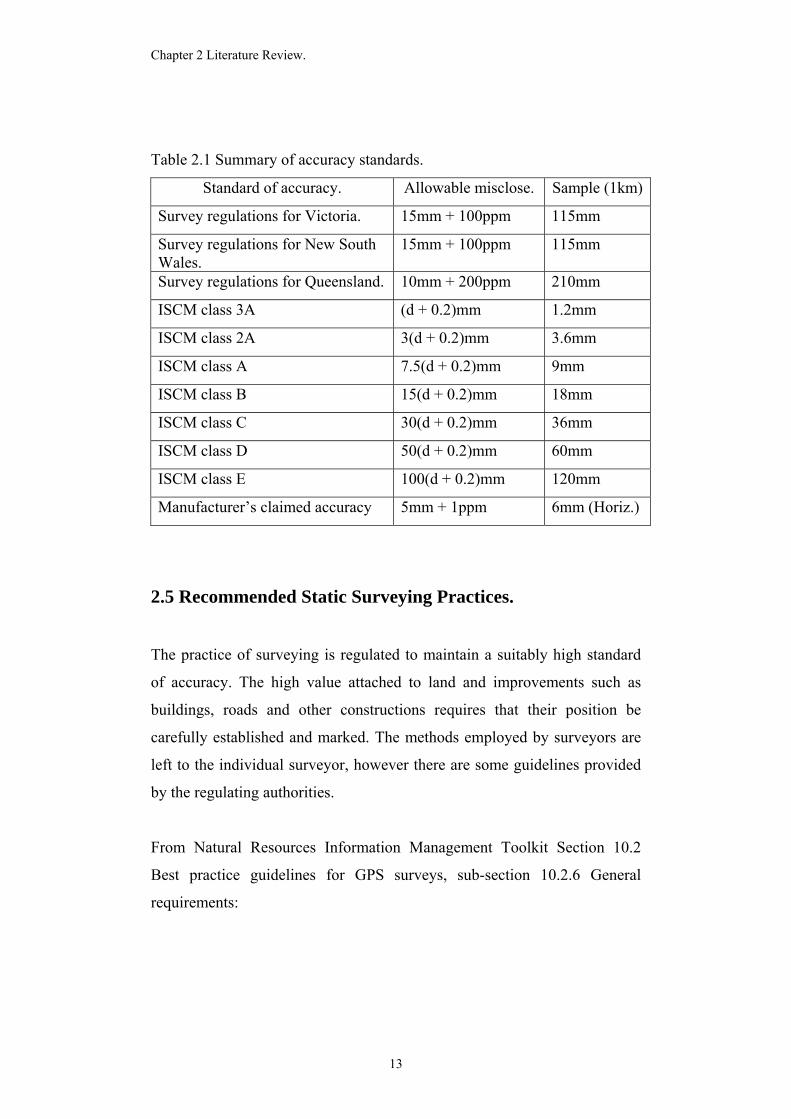
Table 2.1 Summary of accuracy standards.
Standard of accuracy. Allowable misclose. Sample (1km)
Survey regulations for Victoria. 15mm + 100ppm 115mm
Survey regulations for New South Wales.
15mm + 100ppm 115mm
Survey regulations for Queensland. 10mm + 200ppm 210mm
ISCM class 3A (d + 0.2)mm 1.2mm
ISCM class 2A 3(d + 0.2)mm 3.6mm
ISCM class A 7.5(d + 0.2)mm 9mm
ISCM class B 15(d + 0.2)mm 18mm
ISCM class C 30(d + 0.2)mm 36mm
ISCM class D 50(d + 0.2)mm 60mm
ISCM class E 100(d + 0.2)mm 120mm
Manufacturer’s claimed accuracy 5mm + 1ppm 6mm (Horiz.)
2.5 Recommended Static Surveying Practices.
The practice of surveying is regulated to maintain a suitably high standard
of accuracy. The high value attached to land and improvements such as
buildings, roads and other constructions requires that their position be
carefully established and marked. The methods employed by surveyors are
left to the individual surveyor, however there are some guidelines provided
by the regulating authorities.
From Natural Resources Information Management Toolkit Section 10.2
Best practice guidelines for GPS surveys, sub-section 10.2.6 General
requirements:
13
Chapter 2 Literature Review.
Include recording the point identifier at the time of the observation to ensure
that there is no confusion when processing the observation. The dilution of
precision should be less than 8 to minimise the effect or poor satellite
geometry. Mission planning should be carried out to ensure sufficient
satellites are available (minimum of four). In Australia the elevation mask
should be set at 15 degrees above the horizon (satellites below this elevation
should be disregarded). Known reference marks used should have high
quality coordinates and heights (when required). All field observations
should be recorded on field observation sheets as a reference. Measurements
must form a closed figure, and be connected to at least 2 known marks.
Accuracy should be checked by performing a least squares adjustment of the
observed network, these adjustments should be three dimensional in nature.
From Natural Resources Information Management Toolkit Section 10.2
Best practice guidelines for GPS surveys, sub-section 10.2.6.1 Static
Surveying:
Include keeping observations to a minimum of 30 minutes and in duration.
The recording interval should be 15 or 30 seconds. The satellite geometry
should alter significantly over the course of the observation. The use of
single frequency receivers (such as the Ashtech ProMark2 receivers) should
be kept to short lines for non high precision applications.
It is interesting to note that these recommendations state that single
frequency receivers are suitable only for short baseline observations in non
high precision applications. This project aims to evaluate a range of baseline
measurements (up to fifteen kilometres) for accuracy.
14
Chapter 2 Literature Review.
2.6 Validation Methods for GPS Receivers.
The equipment used for a particular survey is left to the surveyor. Only the
accuracy and precision of the end result is subject to regulation. The
equipment used by a surveyor should be selected and maintained such that it
is capable of producing results that pass the requirements of the regulatory
body. Any testing procedure may be adopted by the surveyor as long as it
can be established that the measurements have been compared to
appropriate standards, and can be made within appropriate accuracy
tolerances (Survey Board Victoria 2006).
There exist two separate tests for evaluating GPS receivers in static mode.
These are the zero baseline test and the test network observation.
2.6.1 Zero Baseline Test.
This can be carried out to check the correct operation of a pair of GPS
receivers, associated antennas/cabling, and data processing software. A
zero baseline test involves connecting two GPS receivers to the same
antenna via an antenna splitter (as recommended by the manufacturer).
The computed baseline should be theoretically equal to zero and any
variation will represent a vector of receiver errors (should give sub
millimetre results).
This is a very simple and inexpensive process which:
- verifies the precision of the GPS receiver measurements,
- proves that the receiver is operating correctly, and also
- validates the processing software (Survey Board Victoria 2006).
15
Chapter 2 Literature Review.
2.6.2 Static Mode Evaluation.
From: Surveyors Registration Board of Victoria, Survey Practice
Handbook, Part 2, Section 12, Subsection 12.1.2 (2006):
A High Accuracy GPS Test Network (Static Techniques)
This can be undertaken to ensure that the operation of GPS receivers,
associated cabling, and data processing software, give high accuracy
baseline/coordinate results. Satellite ephemeris errors, clock biases and
atmospheric effects must be removed or minimised during baseline
processing. Network validation allows GPS equipment to be tested under
realistic field conditions which includes the dynamic nature of the
satellite constellation and the atmosphere (Survey Board Victoria 2006).
The test network should consist of extremely stable ground marks with
almost perfect sky visibility and be of very high precision (e.g. first or
second order). The stations should be coordinated in both the local
geodetic system (AGD/GDA φ, λ, h or x, y, z) and plane projection
(MGA E, N and AHD elevations). Observed baselines should have a
variety of baseline lengths and directions, and consist of points with
varying elevations (to check for the correct modeling of the atmosphere
as well as geoid determination to obtain AHD values) (Survey Board
Victoria 2006).
After observing the network, the surveyor can process the data to
produce a network of vectors. These vectors can then be reviewed,
adjusted and analysed against the known mark coordinates.
16
Chapter 2 Literature Review.
As all marks observed in this project have known horizontal coordinates
and known elevation the observed vectors will be analysed against the
coordinate differences for the each pair of permanent survey marks.
2.7 Satellite orbit period.
Ideally the test observations would be carried at the same time such that the
satellite configuration in the sky was the same (eliminating a further
variable in the results). This was not possible, as the author only had access
to two receivers.
It was necessary to know the time it takes for the satellites to complete 1
orbit. This is so that the observations can be taken at the same point in the
satellite orbit to keep the satellite configuration close to constant for all
observations.
Their orbital period is approximately 11hrs 58mins, so that each satellite
makes two revolutions in one sidereal day (the period taken for the earth to
complete one rotation about its axis with respect to the stars). (SNAP-
UNSW 1999c).
At the end of a sidereal day (approximately 23hrs 56mins in length) the
satellites are again over the same position on earth. (SNAP-UNSW 1999c).
Reckoned in terms of a solar day (24hrs in length), the satellites are in the
same position in the sky about four (4) minutes earlier each day. (SNAP-
UNSW 1999c).
If the observations are made as close to 23 hours 56 minutes apart then the
satellite configuration should stay reasonably constant.
17
Chapter 2 Literature Review.
2.8 Control Mark Accuracy.
The coordinates assigned to a survey station have accuracies dependent on
the survey used to connect them to the network. (ICSM 2004). The survey
marks used in this project are supplied with 3rd order coordinates and as
such have an error tolerance attached to them. The ISCM sets the order of a
survey mark according to the class of the survey used to connect the mark
and the fit of this connection with the rest of the network.
Order is a function of the Class of a survey, the conformity of the new
survey data with an existing network coordinate set and the precision of any
transformation process required to convert results from one datum to
another.
(ICSM 2004).
The order assigned to the stations in a new survey network following
constraint of that network to the existing coordinate set may be;
a) not higher than the order of existing stations constraining that
network, and
b) not higher than the class assigned to that survey.
The highest order that may be assigned to a station from a survey of a given
class is shown (ICSM 2004).
18
Chapter 2 Literature Review.
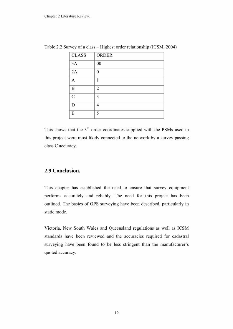
Table 2.2 Survey of a class – Highest order relationship (ICSM, 2004)
CLASS ORDER
3A 00
2A 0
A 1
B 2
C 3
D 4
E 5
This shows that the 3rd order coordinates supplied with the PSMs used in
this project were most likely connected to the network by a survey passing
class C accuracy.
2.9 Conclusion.
This chapter has established the need to ensure that survey equipment
performs accurately and reliably. The need for this project has been
outlined. The basics of GPS surveying have been described, particularly in
static mode.
Victoria, New South Wales and Queensland regulations as well as ICSM
standards have been reviewed and the accuracies required for cadastral
surveying have been found to be less stringent than the manufacturer’s
quoted accuracy.
19

Chapter 2 Literature Review.
General guidelines for successful GPS observations have been reviewed,
along with more specific recommendations relating to static mode
observations, including equipment test procedures.
The accuracies of coordinates associated with established survey marks
have also been outlined.
20
Chapter 3 Project Methodology.
CHAPTER 3
PROJECT METHODOLOGY
3.1 Introduction.
The methodology of the project has been established by the findings of the
Literature Review. The tests selected to establish that the Ashtech ProMark2
receivers (and associated processing software) were the zero baseline test
and the test network observation.
The performance of a Zero Baseline observation was dependent on the
availability of a splitter connection to allow two receivers to record data
from a single antenna. This piece of equipment was unable to be acquired
during the course of the study and as such, the zero baseline test was not
performed.
The network observations were processed with varied numbers of satellites
(and corresponding variations in DOP’s) and observation times for each
baseline.
The baseline observations were made in the City of Greater Bendigo
spanning the suburbs between Epsom and Kangaroo Flat (see appendix C
for map).
21
Chapter 3 Project Methodology.
3.2 Expectations.
The study is expected to provide a definitive answer as to the achievable
accuracy of results using the Ashtech ProMark2. These results will then be
used to determine what types of survey work the equipment is suitable for,
as well as forming the basis for recommendations about appropriate
observation durations.
3.3 Reference Marks.
The availability of first or second order survey marks in the local area is
very limited. This has meant that the test network will consist of permanent
survey marks with 3rd order coordinated attached to them. The locations of
these marks are illustrated in appendix C.
The survey mark enquirery service accessed at http://land.vic.gov.au/smes
provides a search function (to locate survey marks) as well as providing
sketch plans and coordinates for these marks. The sketch plans for the
permanent marks utilised for this project are included as appendix D.
3.4 Fieldwork.
3.4.2 Network observations.
Each baseline is to be observed for 2 hours at the same time of day on
consecutive days to ensure similar satellite configuration and motion.
22
Chapter 3 Project Methodology.
The procedure for each observation was:
1. Set up over the PSM taking care to ensure that the antenna is level
and directly over the centre of the mark. Measure the height of the
antenna using the Ashtech supplied tape (calibrated for the phase
centre of the antenna).
2. Turn on the receiver and set as follows:
a. Select static survey mode.
b. Enter point identifier (different for each receiver).
c. Select 30 second observation interval.
d. Enter antenna height.
e. Set units to metres.
3. Leave the receiver running and proceed to the next mark and
repeat the setup procedure.
4. Collect 2 hours of overlapping data.
5. Turn off and pack up the first receiver and return to the first mark
to pack up.
3.6 Analysis.
The post processing and data analysis steps are:
1. Upload data files from receivers to PC for processing.
2. Create files for different baselines, satellite numbers and
observation times. The Ashtech Solutions software package allows
the observation data to be trimmed prior to processing. For each
file the data was trimmed to create an observation of the required
length. The software also allows specific satellites to be removed
from the processed data; satellites were removed to generate files
with 4, 5, 6, and 8 satellites present in the data.
23
Chapter 3 Project Methodology.
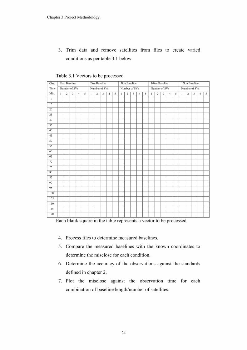
3. Trim data and remove satellites from files to create varied
conditions as per table 3.1 below.
Table 3.1 Vectors to be processed. 1km Baseline 2km Baseline 5km Baseline 10km Baseline 15km Baseline
Number of SVs Number of SVs Number of SVs Number of SVs Number of SVs
Obs.
Time
Min. 1 2 3 4 5 1 2 3 4 5 1 2 3 4 5 1 2 3 4 5 1 2 3 4 5
10
15
20
25
30
35
40
45
50
55
60
65
70
75
80
85
90
95
100
105
110
115
120
Each blank square in the table represents a vector to be processed.
4. Process files to determine measured baselines.
5. Compare the measured baselines with the known coordinates to
determine the misclose for each condition.
6. Determine the accuracy of the observations against the standards
defined in chapter 2.
7. Plot the misclose against the observation time for each
combination of baseline length/number of satellites.
24
Chapter 3 Project Methodology.
3.7 Data Analysis.
By plotting the misclose against the observation time for each condition it is
possible to see if there is some relationship between the length of the
observation and the achieved accuracy. Then it is also possible to
recommend minimum observation durations for each combination of
number of satellites and baseline length.
The level of accuracy achieved can also be assessed to determine if the
equipment is suitable for use for cadastral (by comparison with survey
regulations) and other work.
If there is an observed correspondence between observation time and
accuracy, and the accuracy can be shown to comply with the regulations,
then a recommended observation time can be determined for each condition.
3.8 Conclusion.
The methodology for this project can be broken down into the following
components:
1. Research information relating to the global positioning system, GPS
surveying, static survey techniques, accuracy requirements, reference
mark accuracies and GPS receiver evaluation techniques.
2. Field observations were made measuring baselines between
coordinated permanent survey marks. The baselines measured were
be of varied lengths.
25

Chapter 3 Project Methodology.
3. The recorded data was processed to produce resultant baseline
vectors which were then compared to the known coordinates for the
stations to determine the accuracy for each set of conditions.
4. Recommendations were made as to the observation time required for
variations in baseline length, number of visible satellites and dilutions
of precision.
26
Chapter 4 Results.
CHAPTER 4
RESULTS
4.1 Introduction.
The literature review identified two tests to determine whether or not a GPS
survey system is performing as it should. The first of these was the zero
baseline test which was not performed due to the lack of a cable splitter.
The results presented in this chapter are for the second test, the observation
of known survey points. The observations performed form a closed loop to
provide a further check on the system performance.
The author has decided that, in the absence of the zero baseline test, if the
results achieved around the baseline network are suitably accurate then the
system can be said to be functioning correctly.
4.2 Results compared with Known Coordinates.
4.2.1 Permanent Mark Coordinates.
The permanent marks used to define the baselines for this test each carry
assigned third order MGA coordinates (see appendix D). These
coordinates are shown in table 4.1 below.
27
Chapter 4 Results.
Table 4.1 Known PSM coordinates. Permanent Mark. Easting (Zone 55) Northing (Zone 55) RL (AHD)
PM22 260402.546 5935515.250 182.374
PM56 253575.556 5921434.301 273.460
PM872 260964.054 5928409.319 243.520
PM1013 260746.861 5934403.227 186.827
PM1927 260082.548 5933428.672 190.217
The baselines measured were:
1. PM1013 to PM22 approximately one kilometre.
2. PM22 to PM1927 approximately two kilometres.
3. PM1927 to PM872 approximately five kilometres.
4. PM872 to PM56 approximately ten kilometres.
5. PM56 to PM1013 approximately fifteen kilometres.
The vectors for each baseline 1 to 5 are expressed as differences in
Easting, Northing and RL in table below.
Table 4.2 Observed vectors calculated from known coordinates. Baseline Δ Easting. Δ Northing. Δ RL
1. -344.315 1112.023 -4.453
2. -319.998 -2086.578 7.843
3. 881.506 -5019.353 53.303
4. -7388.498 -6975.018 29.940
5. 7171.305 12968.926 -86.633
4.2.2 Observed Vectors
The GPS observations were split up as described in chapter 3 to provide
raw data for observations meeting each of the requirements in table 4.3
below.
28
Chapter 4 Results.
Table 4.3 Vectors to be processed. 1km Baseline 2km Baseline 5km Baseline 10km Baseline 15km Baseline
Number of SVs Number of SVs Number of SVs Number of SVs Number of SVs
Obs.
Time
Min. 1 2 3 4 5 1 2 3 4 5 1 2 3 4 5 1 2 3 4 5 1 2 3 4 5
10
15
20
25
30
35
40
45
50
55
60
65
70
75
80
85
90
95
100
105
110
115
120
Each blank square represents a vector to be analysed (total 575).
Each vector was reduced using Ashtech Solutions version 2.60 to provide
ΔE, ΔN and ΔRL for comparison against the vectors in table. The
analysis involved the calculation of 3-dimensional misclose, horizontal
misclose and vertical misclose compared to the permanent mark
coordinates.
29
Chapter 4 Results.
4.2.3 Sample Calculations.
The processed vector was compared against the known vector to provide
miscloses as follows.
The tables 4.4 and 4.5 show the computations conducted to create the
miscloses for each vector.
The columns in these tables can be described thus:
1. Represents the observation duration in minutes.
2. The difference in the Easting measured between the survey marks.
3. The difference in the Northing measured between the survey marks.
4. The difference in the elevation measured between the survey marks.
5. The computed slope distance between the survey marks.
6. The difference between the measured ΔE and the known ΔE.
7. The difference between the measured ΔN and the known ΔN.
8. The difference between the measured ΔRL and the known ΔRL.
9. The misclose of the measured and known vectors in 3 dimensions.
10. The misclose considering only ΔEs and ΔNs (horizontal).
11. The misclose in vertical direction (magnitude of ΔRL).
30
Chapter 4 Results.
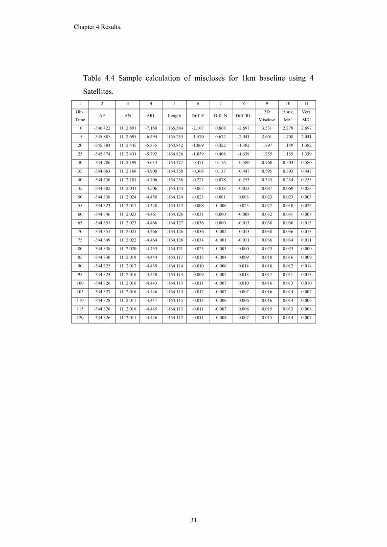
Table 4.4 Sample calculation of miscloses for 1km baseline using 4
Satellites. 1 2 3 4 5 6 7 8 9 10 11
Obs.
Time ΔE ΔN ΔRL Length Diff. E Diff. N Diff. RL
3D
Misclose
Horiz.
M/C
Vert.
M/C
10 -346.422 1112.891 -7.150 1165.584 -2.107 0.868 -2.697 3.531 2.279 2.697
15 -345.885 1112.695 -6.494 1165.233 -1.570 0.672 -2.041 2.661 1.708 2.041
20 -345.384 1112.445 -5.835 1164.842 -1.069 0.422 -1.382 1.797 1.149 1.382
25 -345.374 1112.431 -5.792 1164.826 -1.059 0.408 -1.339 1.755 1.135 1.339
30 -344.786 1112.199 -5.033 1164.427 -0.471 0.176 -0.580 0.768 0.503 0.580
35 -344.683 1112.160 -4.900 1164.358 -0.368 0.137 -0.447 0.595 0.393 0.447
40 -344.536 1112.101 -4.706 1164.258 -0.221 0.078 -0.253 0.345 0.234 0.253
45 -344.382 1112.041 -4.506 1164.154 -0.067 0.018 -0.053 0.087 0.069 0.053
50 -344.338 1112.024 -4.450 1164.124 -0.023 0.001 0.003 0.023 0.023 0.003
55 -344.323 1112.017 -4.428 1164.113 -0.008 -0.006 0.025 0.027 0.010 0.025
60 -344.346 1112.023 -4.461 1164.126 -0.031 0.000 -0.008 0.032 0.031 0.008
65 -344.351 1112.023 -4.466 1164.127 -0.036 0.000 -0.013 0.038 0.036 0.013
70 -344.351 1112.021 -4.466 1164.126 -0.036 -0.002 -0.013 0.038 0.036 0.013
75 -344.349 1112.022 -4.464 1164.126 -0.034 -0.001 -0.011 0.036 0.034 0.011
80 -344.338 1112.020 -4.453 1164.121 -0.023 -0.003 0.000 0.023 0.023 0.000
85 -344.330 1112.019 -4.444 1164.117 -0.015 -0.004 0.009 0.018 0.016 0.009
90 -344.325 1112.017 -4.439 1164.114 -0.010 -0.006 0.014 0.018 0.012 0.014
95 -344.324 1112.016 -4.440 1164.113 -0.009 -0.007 0.013 0.017 0.011 0.013
100 -344.326 1112.016 -4.443 1164.113 -0.011 -0.007 0.010 0.016 0.013 0.010
105 -344.327 1112.016 -4.446 1164.114 -0.012 -0.007 0.007 0.016 0.014 0.007
110 -344.328 1112.017 -4.447 1164.115 -0.013 -0.006 0.006 0.016 0.014 0.006
115 -344.326 1112.016 -4.445 1164.113 -0.011 -0.007 0.008 0.015 0.013 0.008
120 -344.326 1112.015 -4.446 1164.112 -0.011 -0.008 0.007 0.015 0.014 0.007
31
Chapter 4 Results.
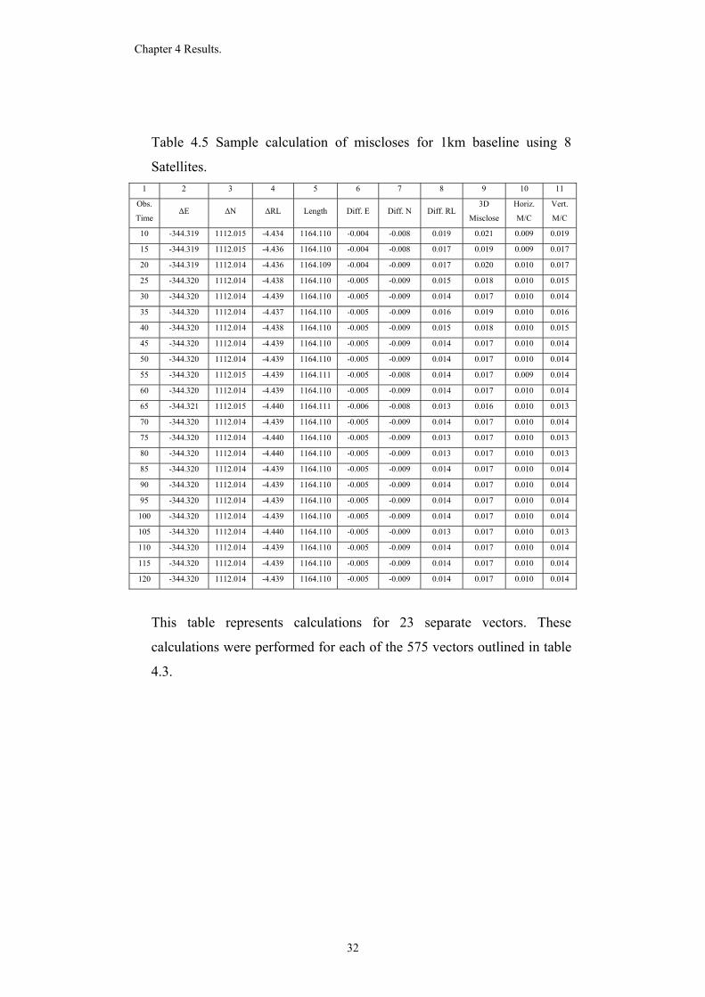
Table 4.5 Sample calculation of miscloses for 1km baseline using 8
Satellites. 1 2 3 4 5 6 7 8 9 10 11
Obs.
Time ΔE ΔN ΔRL Length Diff. E Diff. N Diff. RL
3D
Misclose
Horiz.
M/C
Vert.
M/C
10 -344.319 1112.015 -4.434 1164.110 -0.004 -0.008 0.019 0.021 0.009 0.019
15 -344.319 1112.015 -4.436 1164.110 -0.004 -0.008 0.017 0.019 0.009 0.017
20 -344.319 1112.014 -4.436 1164.109 -0.004 -0.009 0.017 0.020 0.010 0.017
25 -344.320 1112.014 -4.438 1164.110 -0.005 -0.009 0.015 0.018 0.010 0.015
30 -344.320 1112.014 -4.439 1164.110 -0.005 -0.009 0.014 0.017 0.010 0.014
35 -344.320 1112.014 -4.437 1164.110 -0.005 -0.009 0.016 0.019 0.010 0.016
40 -344.320 1112.014 -4.438 1164.110 -0.005 -0.009 0.015 0.018 0.010 0.015
45 -344.320 1112.014 -4.439 1164.110 -0.005 -0.009 0.014 0.017 0.010 0.014
50 -344.320 1112.014 -4.439 1164.110 -0.005 -0.009 0.014 0.017 0.010 0.014
55 -344.320 1112.015 -4.439 1164.111 -0.005 -0.008 0.014 0.017 0.009 0.014
60 -344.320 1112.014 -4.439 1164.110 -0.005 -0.009 0.014 0.017 0.010 0.014
65 -344.321 1112.015 -4.440 1164.111 -0.006 -0.008 0.013 0.016 0.010 0.013
70 -344.320 1112.014 -4.439 1164.110 -0.005 -0.009 0.014 0.017 0.010 0.014
75 -344.320 1112.014 -4.440 1164.110 -0.005 -0.009 0.013 0.017 0.010 0.013
80 -344.320 1112.014 -4.440 1164.110 -0.005 -0.009 0.013 0.017 0.010 0.013
85 -344.320 1112.014 -4.439 1164.110 -0.005 -0.009 0.014 0.017 0.010 0.014
90 -344.320 1112.014 -4.439 1164.110 -0.005 -0.009 0.014 0.017 0.010 0.014
95 -344.320 1112.014 -4.439 1164.110 -0.005 -0.009 0.014 0.017 0.010 0.014
100 -344.320 1112.014 -4.439 1164.110 -0.005 -0.009 0.014 0.017 0.010 0.014
105 -344.320 1112.014 -4.440 1164.110 -0.005 -0.009 0.013 0.017 0.010 0.013
110 -344.320 1112.014 -4.439 1164.110 -0.005 -0.009 0.014 0.017 0.010 0.014
115 -344.320 1112.014 -4.439 1164.110 -0.005 -0.009 0.014 0.017 0.010 0.014
120 -344.320 1112.014 -4.439 1164.110 -0.005 -0.009 0.014 0.017 0.010 0.014
This table represents calculations for 23 separate vectors. These
calculations were performed for each of the 575 vectors outlined in table
4.3.
32
Chapter 4 Results.
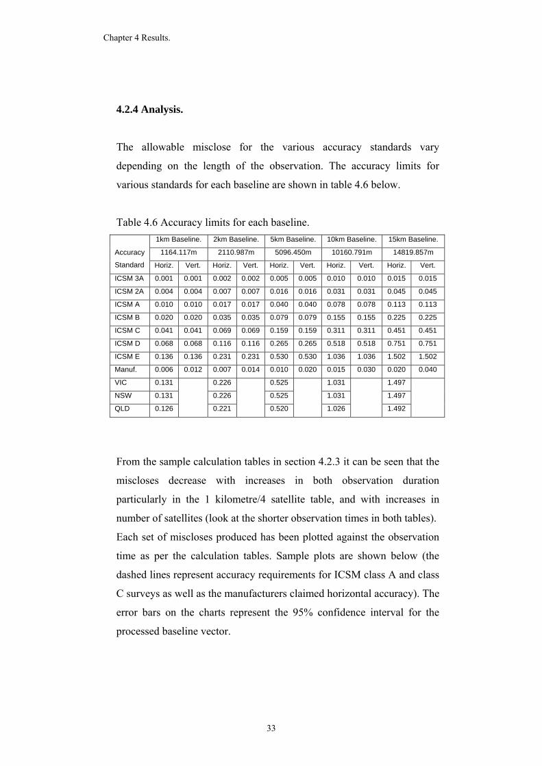
4.2.4 Analysis.
The allowable misclose for the various accuracy standards vary
depending on the length of the observation. The accuracy limits for
various standards for each baseline are shown in table 4.6 below.
Table 4.6 Accuracy limits for each baseline. 1km Baseline. 2km Baseline. 5km Baseline. 10km Baseline. 15km Baseline.
1164.117m 2110.987m 5096.450m 10160.791m 14819.857m Accuracy
Standard Horiz. Vert. Horiz. Vert. Horiz. Vert. Horiz. Vert. Horiz. Vert.
ICSM 3A 0.001 0.001 0.002 0.002 0.005 0.005 0.010 0.010 0.015 0.015
ICSM 2A 0.004 0.004 0.007 0.007 0.016 0.016 0.031 0.031 0.045 0.045
ICSM A 0.010 0.010 0.017 0.017 0.040 0.040 0.078 0.078 0.113 0.113
ICSM B 0.020 0.020 0.035 0.035 0.079 0.079 0.155 0.155 0.225 0.225
ICSM C 0.041 0.041 0.069 0.069 0.159 0.159 0.311 0.311 0.451 0.451
ICSM D 0.068 0.068 0.116 0.116 0.265 0.265 0.518 0.518 0.751 0.751
ICSM E 0.136 0.136 0.231 0.231 0.530 0.530 1.036 1.036 1.502 1.502
Manuf. 0.006 0.012 0.007 0.014 0.010 0.020 0.015 0.030 0.020 0.040
VIC 0.131 0.226 0.525 1.031 1.497
NSW 0.131 0.226 0.525 1.031 1.497
QLD 0.126 0.221 0.520 1.026 1.492
From the sample calculation tables in section 4.2.3 it can be seen that the
miscloses decrease with increases in both observation duration
particularly in the 1 kilometre/4 satellite table, and with increases in
number of satellites (look at the shorter observation times in both tables).
Each set of miscloses produced has been plotted against the observation
time as per the calculation tables. Sample plots are shown below (the
dashed lines represent accuracy requirements for ICSM class A and class
C surveys as well as the manufacturers claimed horizontal accuracy). The
error bars on the charts represent the 95% confidence interval for the
processed baseline vector.
33
Chapter 4 Results.
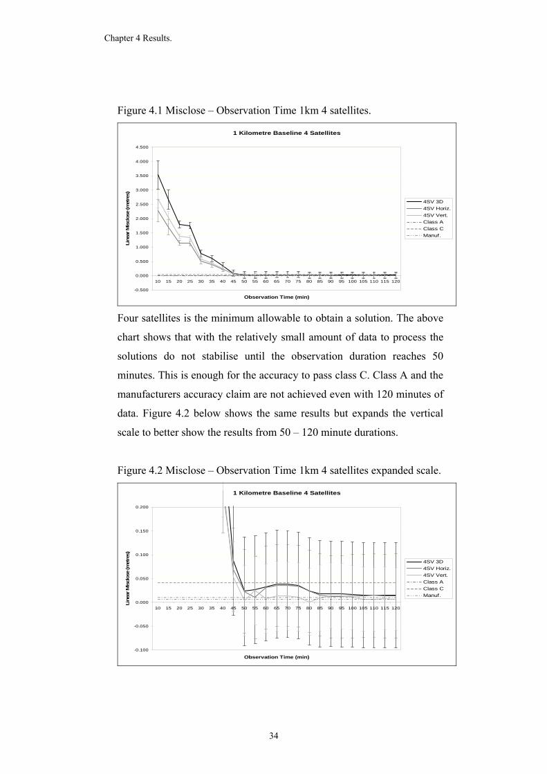
Figure 4.1 Misclose – Observation Time 1km 4 satellites.
1 Kilometre Baseline 4 Satellites
-0.500
0.000
0.500
1.000
1.500
2.000
2.500
3.000
3.500
4.000
4.500
10 15 20 25 30 35 40 45 50 55 60 65 70 75 80 85 90 95 100 105 110 115 120
Observation Time (min)
Line
ar M
iscl
ose
(met
res)
4SV 3D4SV Horiz.4SV Vert.Class AClass CManuf.
Four satellites is the minimum allowable to obtain a solution. The above
chart shows that with the relatively small amount of data to process the
solutions do not stabilise until the observation duration reaches 50
minutes. This is enough for the accuracy to pass class C. Class A and the
manufacturers accuracy claim are not achieved even with 120 minutes of
data. Figure 4.2 below shows the same results but expands the vertical
scale to better show the results from 50 – 120 minute durations.
Figure 4.2 Misclose – Observation Time 1km 4 satellites expanded scale.
1 Kilometre Baseline 4 Satellites
-0.100
-0.050
0.000
0.050
0.100
0.150
0.200
10 15 20 25 30 35 40 45 50 55 60 65 70 75 80 85 90 95 100 105 110 115 120
Observation Time (min)
Line
ar M
iscl
ose
(met
res)
4SV 3D4SV Horiz.4SV Vert.Class AClass CManuf.
34
Chapter 4 Results.
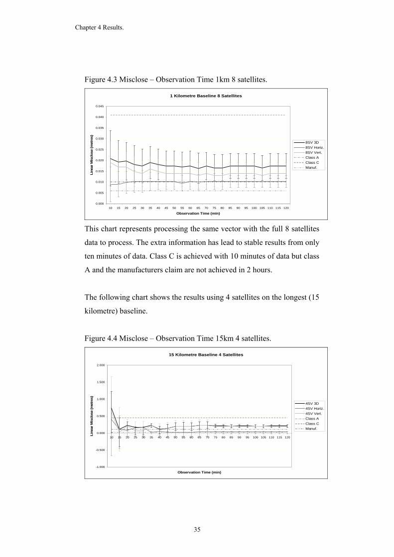
Figure 4.3 Misclose – Observation Time 1km 8 satellites.
1 Kilometre Baseline 8 Satellites
0.000
0.005
0.010
0.015
0.020
0.025
0.030
0.035
0.040
0.045
10 15 20 25 30 35 40 45 50 55 60 65 70 75 80 85 90 95 100 105 110 115 120
Observation Time (min)
Line
ar M
iscl
ose
(met
res)
8SV 3D8SV Horiz.8SV Vert.Class AClass CManuf.
This chart represents processing the same vector with the full 8 satellites
data to process. The extra information has lead to stable results from only
ten minutes of data. Class C is achieved with 10 minutes of data but class
A and the manufacturers claim are not achieved in 2 hours.
The following chart shows the results using 4 satellites on the longest (15
kilometre) baseline.
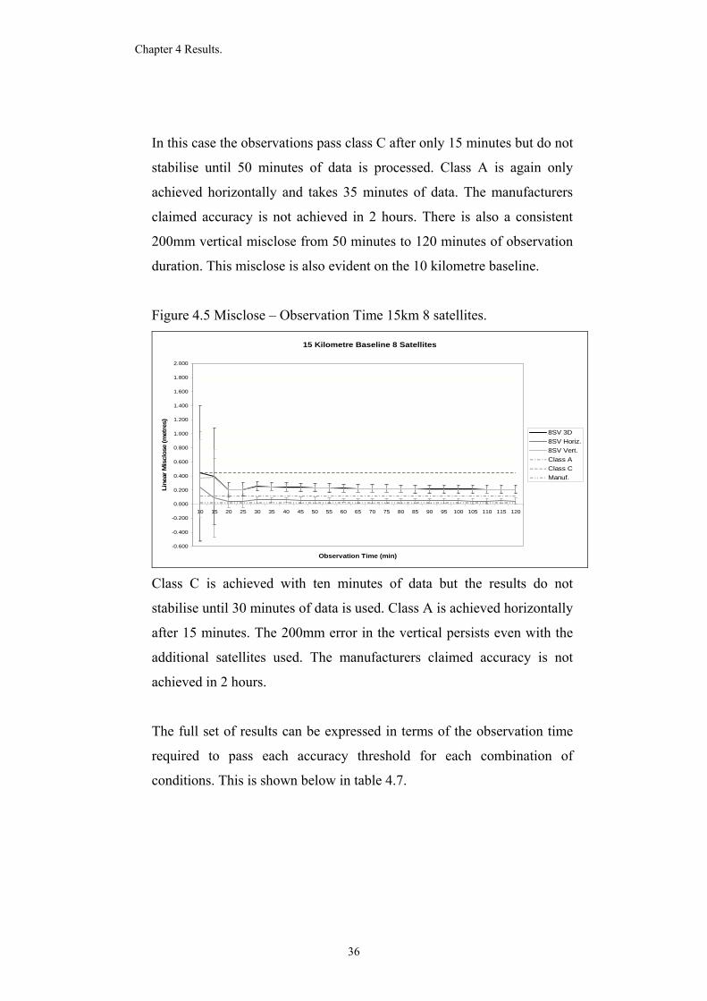
Figure 4.4 Misclose – Observation Time 15km 4 satellites.
15 Kilometre Baseline 4 Satellites
-1.000
-0.500
0.000
0.500
1.000
1.500
2.000
10 15 20 25 30 35 40 45 50 55 60 65 70 75 80 85 90 95 100 105 110 115 120
Observation Time (min)
Line
ar M
iscl
ose
(met
res)
4SV 3D4SV Horiz.4SV Vert.Class AClass CManuf.
35
Chapter 4 Results.
In this case the observations pass class C after only 15 minutes but do not
stabilise until 50 minutes of data is processed. Class A is again only
achieved horizontally and takes 35 minutes of data. The manufacturers
claimed accuracy is not achieved in 2 hours. There is also a consistent
200mm vertical misclose from 50 minutes to 120 minutes of observation
duration. This misclose is also evident on the 10 kilometre baseline.
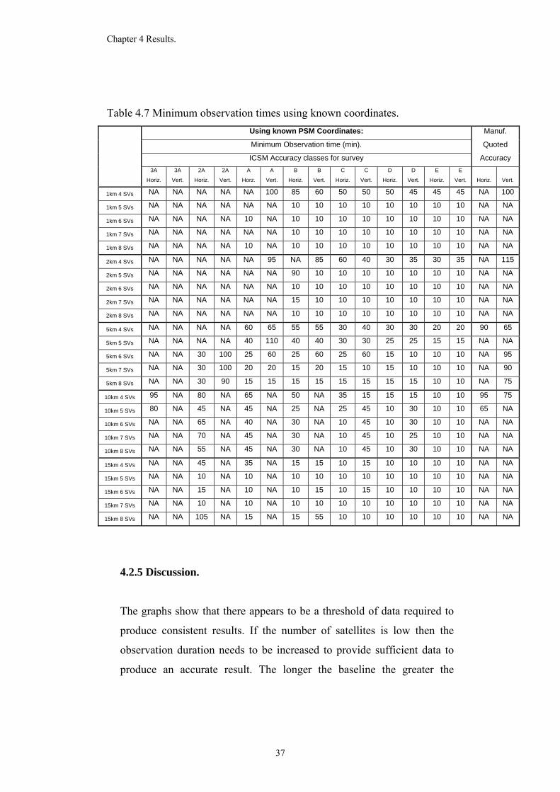
Figure 4.5 Misclose – Observation Time 15km 8 satellites.
15 Kilometre Baseline 8 Satellites
-0.600
-0.400
-0.200
0.000
0.200
0.400
0.600
0.800
1.000
1.200
1.400
1.600
1.800
2.000
10 15 20 25 30 35 40 45 50 55 60 65 70 75 80 85 90 95 100 105 110 115 120
Observation Time (min)
Line
ar M
iscl
ose
(met
res)
8SV 3D8SV Horiz.8SV Vert.Class AClass CManuf.
Class C is achieved with ten minutes of data but the results do not
stabilise until 30 minutes of data is used. Class A is achieved horizontally
after 15 minutes. The 200mm error in the vertical persists even with the
additional satellites used. The manufacturers claimed accuracy is not
achieved in 2 hours.
The full set of results can be expressed in terms of the observation time
required to pass each accuracy threshold for each combination of
conditions. This is shown below in table 4.7.
36
Chapter 4 Results.
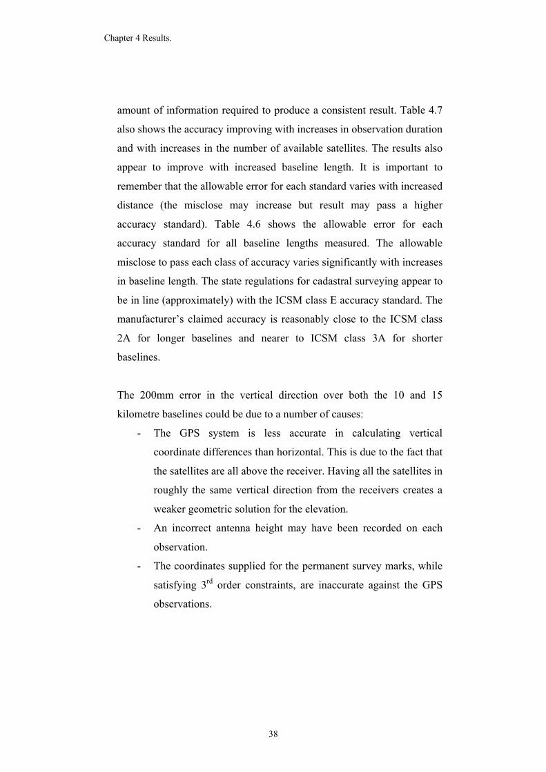
Table 4.7 Minimum observation times using known coordinates. Using known PSM Coordinates: Manuf.
Minimum Observation time (min). Quoted
ICSM Accuracy classes for survey Accuracy
3A
Horiz.
3A
Vert.
2A
Horiz.
2A
Vert.
A
Horz.
A
Vert.
B
Horiz.
B
Vert.
C
Horiz.
C
Vert.
D
Horiz.
D
Vert.
E
Horiz.
E
Vert. Horiz. Vert.
1km 4 SVs NA NA NA NA NA 100 85 60 50 50 50 45 45 45 NA 100
1km 5 SVs NA NA NA NA NA NA 10 10 10 10 10 10 10 10 NA NA
1km 6 SVs NA NA NA NA 10 NA 10 10 10 10 10 10 10 10 NA NA
1km 7 SVs NA NA NA NA NA NA 10 10 10 10 10 10 10 10 NA NA
1km 8 SVs NA NA NA NA 10 NA 10 10 10 10 10 10 10 10 NA NA
2km 4 SVs NA NA NA NA NA 95 NA 85 60 40 30 35 30 35 NA 115
2km 5 SVs NA NA NA NA NA NA 90 10 10 10 10 10 10 10 NA NA
2km 6 SVs NA NA NA NA NA NA 10 10 10 10 10 10 10 10 NA NA
2km 7 SVs NA NA NA NA NA NA 15 10 10 10 10 10 10 10 NA NA
2km 8 SVs NA NA NA NA NA NA 10 10 10 10 10 10 10 10 NA NA
5km 4 SVs NA NA NA NA 60 65 55 55 30 40 30 30 20 20 90 65
5km 5 SVs NA NA NA NA 40 110 40 40 30 30 25 25 15 15 NA NA
5km 6 SVs NA NA 30 100 25 60 25 60 25 60 15 10 10 10 NA 95
5km 7 SVs NA NA 30 100 20 20 15 20 15 10 15 10 10 10 NA 90
5km 8 SVs NA NA 30 90 15 15 15 15 15 15 15 15 10 10 NA 75
10km 4 SVs 95 NA 80 NA 65 NA 50 NA 35 15 15 15 10 10 95 75
10km 5 SVs 80 NA 45 NA 45 NA 25 NA 25 45 10 30 10 10 65 NA
10km 6 SVs NA NA 65 NA 40 NA 30 NA 10 45 10 30 10 10 NA NA
10km 7 SVs NA NA 70 NA 45 NA 30 NA 10 45 10 25 10 10 NA NA
10km 8 SVs NA NA 55 NA 45 NA 30 NA 10 45 10 30 10 10 NA NA
15km 4 SVs NA NA 45 NA 35 NA 15 15 10 15 10 10 10 10 NA NA
15km 5 SVs NA NA 10 NA 10 NA 10 10 10 10 10 10 10 10 NA NA
15km 6 SVs NA NA 15 NA 10 NA 10 15 10 15 10 10 10 10 NA NA
15km 7 SVs NA NA 10 NA 10 NA 10 10 10 10 10 10 10 10 NA NA
15km 8 SVs NA NA 105 NA 15 NA 15 55 10 10 10 10 10 10 NA NA
4.2.5 Discussion.
The graphs show that there appears to be a threshold of data required to
produce consistent results. If the number of satellites is low then the
observation duration needs to be increased to provide sufficient data to
produce an accurate result. The longer the baseline the greater the
37
Chapter 4 Results.
amount of information required to produce a consistent result. Table 4.7
also shows the accuracy improving with increases in observation duration
and with increases in the number of available satellites. The results also
appear to improve with increased baseline length. It is important to
remember that the allowable error for each standard varies with increased
distance (the misclose may increase but result may pass a higher
accuracy standard). Table 4.6 shows the allowable error for each
accuracy standard for all baseline lengths measured. The allowable
misclose to pass each class of accuracy varies significantly with increases
in baseline length. The state regulations for cadastral surveying appear to
be in line (approximately) with the ICSM class E accuracy standard. The
manufacturer’s claimed accuracy is reasonably close to the ICSM class
2A for longer baselines and nearer to ICSM class 3A for shorter
baselines.
The 200mm error in the vertical direction over both the 10 and 15
kilometre baselines could be due to a number of causes:
- The GPS system is less accurate in calculating vertical
coordinate differences than horizontal. This is due to the fact that
the satellites are all above the receiver. Having all the satellites in
roughly the same vertical direction from the receivers creates a
weaker geometric solution for the elevation.
- An incorrect antenna height may have been recorded on each
observation.
- The coordinates supplied for the permanent survey marks, while
satisfying 3rd order constraints, are inaccurate against the GPS
observations.
38
Chapter 4 Results.
It is unlikely that the antenna height was recorded incorrectly on two
separate days and by approximately the same amount (the error occurred
on both the 10km and 15 km baselines recorded 24 hours apart).
The other possibilities can be tested by examining the closure of the
traverse loop. If the misclose around the loop is small then the PSM
coordinates are likely to blame. If the misclose is large then the GPS
system may be the source of the error.
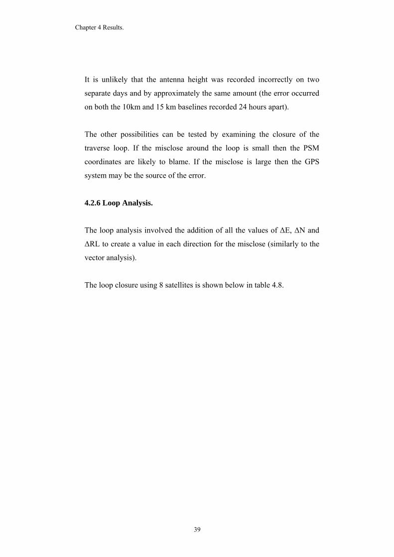
4.2.6 Loop Analysis.
The loop analysis involved the addition of all the values of ΔE, ΔN and
ΔRL to create a value in each direction for the misclose (similarly to the
vector analysis).
The loop closure using 8 satellites is shown below in table 4.8.
39
Chapter 4 Results.
Table 4.8 Loop closure using 8 Satellites.
Misclose
ΔE ΔN ΔRL
3D
Misclose
Horiz.
Misclose
Vert.
Misclose
0.210 0.310 0.412 0.557 0.374 0.412
-0.021 0.189 -0.095 0.213 0.190 0.095
-0.143 0.185 -0.444 0.502 0.234 0.444
-0.164 0.094 -0.330 0.380 0.189 0.330
-0.003 0.071 -0.132 0.150 0.071 0.132
-0.018 0.037 -0.101 0.109 0.041 0.101
0.112 0.029 -0.107 0.158 0.116 0.107
0.015 -0.021 0.052 0.058 0.026 0.052
0.013 -0.021 0.047 0.053 0.025 0.047
0.014 -0.020 0.046 0.052 0.024 0.046
0.016 -0.022 0.040 0.048 0.027 0.040
0.015 -0.020 0.039 0.046 0.025 0.039
0.016 -0.020 0.040 0.047 0.026 0.040
0.015 -0.019 0.038 0.045 0.024 0.038
0.015 -0.019 0.035 0.043 0.024 0.035
0.014 -0.019 0.033 0.041 0.024 0.033
0.013 -0.019 0.029 0.037 0.023 0.029
0.013 -0.019 0.030 0.038 0.023 0.030
0.013 -0.018 0.029 0.037 0.022 0.029
0.013 -0.007 0.029 0.033 0.015 0.029
0.012 -0.008 0.025 0.029 0.014 0.025
0.011 -0.016 0.025 0.032 0.019 0.025
0.011 -0.014 0.024 0.030 0.018 0.024
The misclose for the closed loop of vectors expressed in terms of Easting
Northing and ΔRL are:
- ΔE = 11mm
- ΔN = 14mm
- ΔRL = 24mm
40
Chapter 4 Results.
This level of accuracy, over ~33km of observed traverse loop, suggests
that an error of 200mm vertically in 2 vectors is unlikely. The more
likely cause is an error in the coordinates of one or both of these marks.
Note: The coordinates supplied are only 3rd order and the difference of
200mm over the 10km baseline is acceptable at this accuracy tolerance.
4.3 Results compared with Adjusted Coordinates.
The closures suggest that the GPS survey may be more accurate than the 3rd
order coordinates associated with the permanent survey marks. The full
observations, using 120 minutes of data and all ten visible satellites were
then processed and the network adjusted to provide a new set of base
coordinates (the adjustment passed the processing software’s chi-square test
at the ICSM class 2A accuracy level).
The observed baseline analysis will now be carried out against these new
adjusted PSM coordinates. This method is not recommended by the author
as essentially the observations are being analysed against observation data.
However, to get around the inaccuracy of the permanent marks used there
was no alternative method to establish the overall accuracy of the results.
41
Chapter 4 Results.
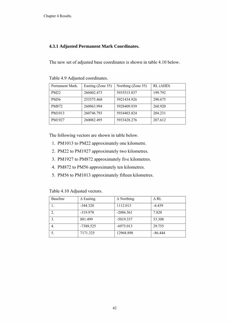
4.3.1 Adjusted Permanent Mark Coordinates.
The new set of adjusted base coordinates is shown in table 4.10 below.
Table 4.9 Adjusted coordinates. Permanent Mark. Easting (Zone 55) Northing (Zone 55) RL (AHD)
PM22 260402.473 5935515.837 199.792
PM56 253575.468 5921434.926 290.675
PM872 260963.994 5928409.939 260.920
PM1013 260746.793 5934403.824 204.231
PM1927 260082.495 5933428.276 207.612
The following vectors are shown in table below.
1. PM1013 to PM22 approximately one kilometre.
2. PM22 to PM1927 approximately two kilometres.
3. PM1927 to PM872 approximately five kilometres.
4. PM872 to PM56 approximately ten kilometres.
5. PM56 to PM1013 approximately fifteen kilometres.
Table 4.10 Adjusted vectors. Baseline Δ Easting. Δ Northing. Δ RL
1. -344.320 1112.013 -4.439
2. -319.978 -2086.561 7.820
3. 881.499 -5019.337 53.308
4. -7388.525 -6975.013 29.755
5. 7171.325 12968.898 -86.444
42
Chapter 4 Results.
4.3.2 Analysis.
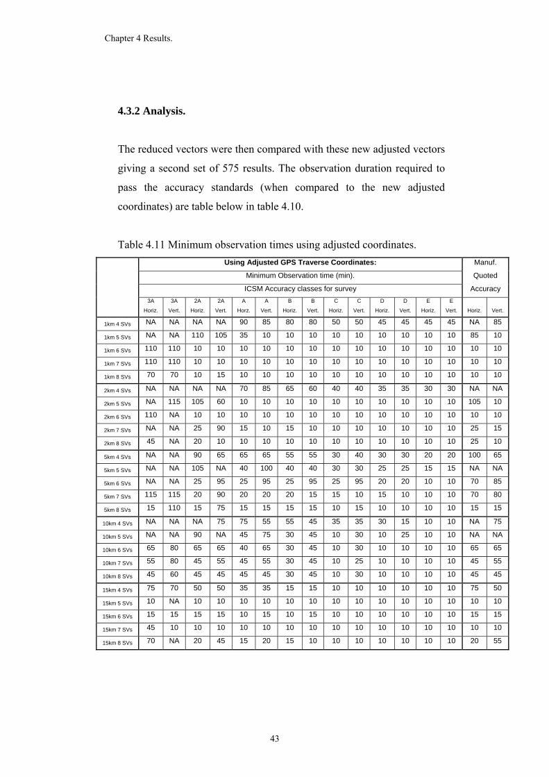
The reduced vectors were then compared with these new adjusted vectors
giving a second set of 575 results. The observation duration required to
pass the accuracy standards (when compared to the new adjusted
coordinates) are table below in table 4.10.
Table 4.11 Minimum observation times using adjusted coordinates. Using Adjusted GPS Traverse Coordinates: Manuf.
Minimum Observation time (min). Quoted
ICSM Accuracy classes for survey Accuracy
3A
Horiz.
3A
Vert.
2A
Horiz.
2A
Vert.
A
Horz.
A
Vert.
B
Horiz.
B
Vert.
C
Horiz.
C
Vert.
D
Horiz.
D
Vert.
E
Horiz.
E
Vert. Horiz. Vert.
1km 4 SVs NA NA NA NA 90 85 80 80 50 50 45 45 45 45 NA 85
1km 5 SVs NA NA 110 105 35 10 10 10 10 10 10 10 10 10 85 10
1km 6 SVs 110 110 10 10 10 10 10 10 10 10 10 10 10 10 10 10
1km 7 SVs 110 110 10 10 10 10 10 10 10 10 10 10 10 10 10 10
1km 8 SVs 70 70 10 15 10 10 10 10 10 10 10 10 10 10 10 10
2km 4 SVs NA NA NA NA 70 85 65 60 40 40 35 35 30 30 NA NA
2km 5 SVs NA 115 105 60 10 10 10 10 10 10 10 10 10 10 105 10
2km 6 SVs 110 NA 10 10 10 10 10 10 10 10 10 10 10 10 10 10
2km 7 SVs NA NA 25 90 15 10 15 10 10 10 10 10 10 10 25 15
2km 8 SVs 45 NA 20 10 10 10 10 10 10 10 10 10 10 10 25 10
5km 4 SVs NA NA 90 65 65 65 55 55 30 40 30 30 20 20 100 65
5km 5 SVs NA NA 105 NA 40 100 40 40 30 30 25 25 15 15 NA NA
5km 6 SVs NA NA 25 95 25 95 25 95 25 95 20 20 10 10 70 85
5km 7 SVs 115 115 20 90 20 20 20 15 15 10 15 10 10 10 70 80
5km 8 SVs 15 110 15 75 15 15 15 15 10 15 10 10 10 10 15 15
10km 4 SVs NA NA NA 75 75 55 55 45 35 35 30 15 10 10 NA 75
10km 5 SVs NA NA 90 NA 45 75 30 45 10 30 10 25 10 10 NA NA
10km 6 SVs 65 80 65 65 40 65 30 45 10 30 10 10 10 10 65 65
10km 7 SVs 55 80 45 55 45 55 30 45 10 25 10 10 10 10 45 55
10km 8 SVs 45 60 45 45 45 45 30 45 10 30 10 10 10 10 45 45
15km 4 SVs 75 70 50 50 35 35 15 15 10 10 10 10 10 10 75 50
15km 5 SVs 10 NA 10 10 10 10 10 10 10 10 10 10 10 10 10 10
15km 6 SVs 15 15 15 15 10 15 10 15 10 10 10 10 10 10 15 15
15km 7 SVs 45 10 10 10 10 10 10 10 10 10 10 10 10 10 10 10
15km 8 SVs 70 NA 20 45 15 20 15 10 10 10 10 10 10 10 20 55
43
Chapter 4 Results.
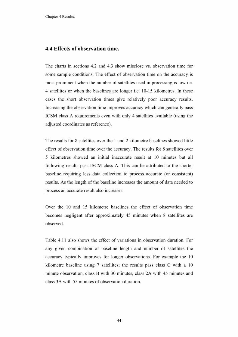
4.4 Effects of observation time.
The charts in sections 4.2 and 4.3 show misclose vs. observation time for
some sample conditions. The effect of observation time on the accuracy is
most prominent when the number of satellites used in processing is low i.e.
4 satellites or when the baselines are longer i.e. 10-15 kilometres. In these
cases the short observation times give relatively poor accuracy results.
Increasing the observation time improves accuracy which can generally pass
ICSM class A requirements even with only 4 satellites available (using the
adjusted coordinates as reference).
The results for 8 satellites over the 1 and 2 kilometre baselines showed little
effect of observation time over the accuracy. The results for 8 satellites over
5 kilometres showed an initial inaccurate result at 10 minutes but all
following results pass ISCM class A. This can be attributed to the shorter
baseline requiring less data collection to process accurate (or consistent)
results. As the length of the baseline increases the amount of data needed to
process an accurate result also increases.
Over the 10 and 15 kilometre baselines the effect of observation time
becomes negligent after approximately 45 minutes when 8 satellites are
observed.
Table 4.11 also shows the effect of variations in observation duration. For
any given combination of baseline length and number of satellites the
accuracy typically improves for longer observations. For example the 10
kilometre baseline using 7 satellites; the results pass class C with a 10
minute observation, class B with 30 minutes, class 2A with 45 minutes and
class 3A with 55 minutes of observation duration.
44
Chapter 4 Results.
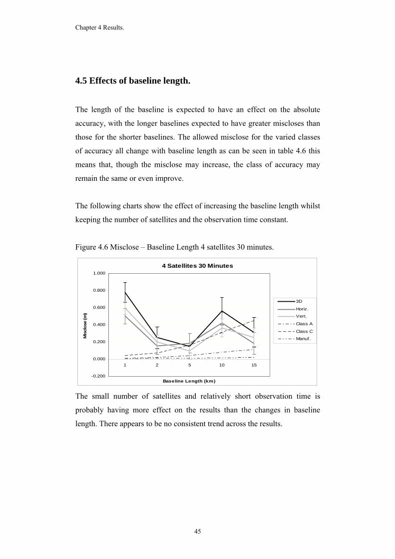
4.5 Effects of baseline length.
The length of the baseline is expected to have an effect on the absolute
accuracy, with the longer baselines expected to have greater miscloses than
those for the shorter baselines. The allowed misclose for the varied classes
of accuracy all change with baseline length as can be seen in table 4.6 this
means that, though the misclose may increase, the class of accuracy may
remain the same or even improve.
The following charts show the effect of increasing the baseline length whilst
keeping the number of satellites and the observation time constant.
Figure 4.6 Misclose – Baseline Length 4 satellites 30 minutes.
4 Satellites 30 Minutes
-0.200
0.000
0.200
0.400
0.600
0.800
1.000
1 2 5 10 15
Baseline Length (km)
Mis
clos
e (m
)
3D
Horiz.
Vert.
Class A
Class C
Manuf.
The small number of satellites and relatively short observation time is
probably having more effect on the results than the changes in baseline
length. There appears to be no consistent trend across the results.
45
Chapter 4 Results.
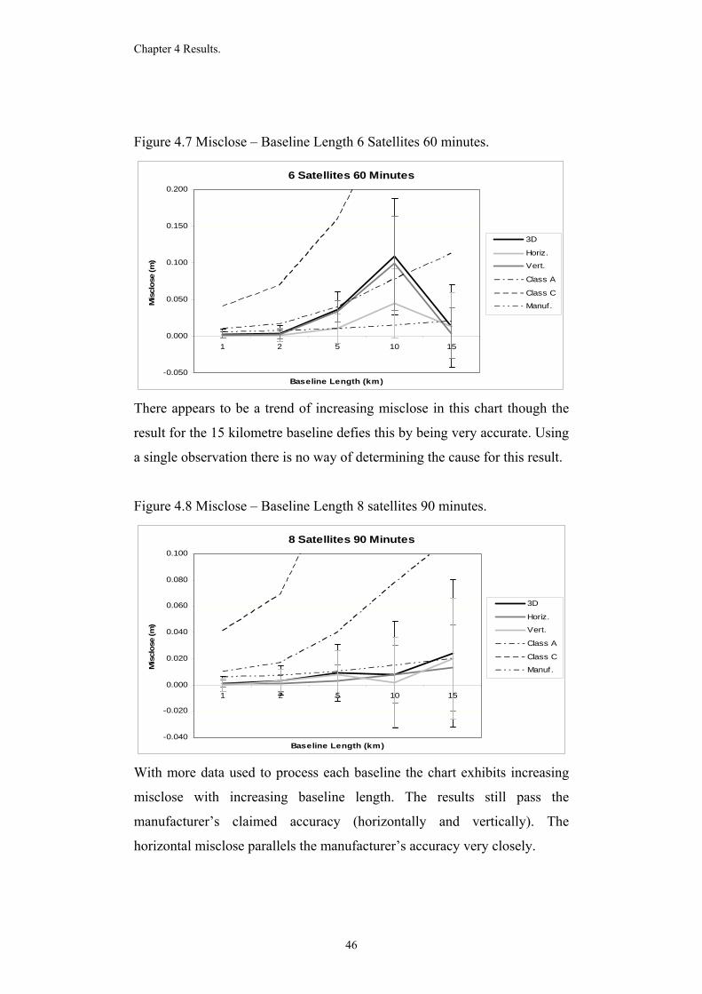
Figure 4.7 Misclose – Baseline Length 6 Satellites 60 minutes.
6 Satellites 60 Minutes
-0.050
0.000
0.050
0.100
0.150
0.200
1 2 5 10 15
Baseline Length (km)
Mis
clos
e (m
)
3D
Horiz.
Vert.
Class A
Class C
Manuf.
There appears to be a trend of increasing misclose in this chart though the
result for the 15 kilometre baseline defies this by being very accurate. Using
a single observation there is no way of determining the cause for this result.
Figure 4.8 Misclose – Baseline Length 8 satellites 90 minutes.
8 Satellites 90 Minutes
-0.040
-0.020
0.000
0.020
0.040
0.060
0.080
0.100
1 2 5 10 15
Baseline Length (km)
Mis
clos
e (m
)
3D
Horiz.
Vert.
Class A
Class C
Manuf.
With more data used to process each baseline the chart exhibits increasing
misclose with increasing baseline length. The results still pass the
manufacturer’s claimed accuracy (horizontally and vertically). The
horizontal misclose parallels the manufacturer’s accuracy very closely.
46
Chapter 4 Results.
Figure 4.9 Misclose – Baseline Length 8 satellites 120 minutes.
8 Satellites 120 Minutes
-0.040
-0.020
0.000
0.020
0.040
0.060
0.080
1 2 5 10 15
Baseline Length (km)
Mis
clos
e (m
)
3D
Horiz.
Vert.
Class A
Class C
Manuf.
Once again with the greater amount of data processed the chart shows
increasing misclose with increasing baseline length. The accuracy relative to
the manufacturer’s claims seems to worsen with baseline length (the
miscloses converge with the manufacturer’s claimed accuracy).
4.6 Effects of number of available satellites.
The minimum number of satellites required to fix the baseline is four, each
additional satellite provides extra information that should enable more
accurate results to be determined. The effect of using more satellites should
also enable more accurate results to be produced using shorter observation
durations.
The following charts show the resultant misclose against number of
satellites for a fixed baseline length/observation duration.
47
Chapter 4 Results.
Figure 4.10 Misclose – Number of Satellites 1 kilometre 20 minutes.
1 Kilometre 20 Minutes
-0.500
0.000
0.500
1.000
1.500
2.000
4 5 6 7 8
Number of Satellites
Mis
clos
e (m
)
3D
Horiz.
Vert.
Class A
Class C
Manuf.
This chart shows an initial large misclose but the results using 5 to 8
satellites are difficult to make out. The following chart (Figure 4.) shows the
same results but the vertical scale has been expanded to show the variation
in results using 5 to 8 satellites.
Figure 4.11 Misclose – Number of Satellites 1 kilometre 20 minutes
expanded scale.
1 Kilometre 20 Minutes
-0.010
-0.005
0.000
0.005
0.010
0.015
0.020
4 5 6 7 8
Number of Satellites
Mis
clos
e (m
)
3D
Horiz.
Vert.
Class A
Class C
Manuf.
With a short baseline and short observation time the minimum four satellites
do not provide an accurate result. Using an additional satellite in the
48
Chapter 4 Results.
processing has a dramatic effect with the misclose passing class C.
Increasing the number of satellites to 6 sees the misclose pass class A and
the manufacturer’s claimed accuracy. Additional satellites have little effect
after this point.
Figure 4.12 Misclose – Number of Satellites 10 kilometres 20 minutes.
10 Kilometres 20 Minutes
0.000
0.100
0.200
0.300
0.400
0.500
0.600
0.700
0.800
0.900
1.000
4 5 6 7 8Number of Satellites
Mis
clos
e (m
)
3D
Horiz.
Vert.
Class A
Class C
Manuf.
Maintaining the short observation time but using the longer 10 kilometre
baseline the results still improve with increasing number of satellites,
though ultimately the accuracy is only good enough for class C in the
horizontal direction. It appears that the short observation time is having the
greatest effect over this distance.
49
Chapter 4 Results.
Figure 4.13 Misclose – Number of Satellites 10 kilometres 60 minutes.
10 Kilometres 60 Minutes
-0.050
0.000
0.050
0.100
0.150
0.200
0.250
0.300
4 5 6 7 8
Number of Satellites
Mis
clos
e (m
)
3D
Horiz.
Vert.
Class A
Class C
Manuf.
Using an hour of data, the accuracy improves consistently with each
additional satellite used. Initially the results pass class C improving to pass
class A with the use of 7 satellites and finally achieving the manufacturer’s
claimed accuracy with 8 satellites used.
Figure 4.14 Misclose – Number of Satellites 10 kilometres 120 minutes.
10 Kilometres 120 Minutes
-0.150
-0.100
-0.050
0.000
0.050
0.100
0.150
0.200
4 5 6 7 8
Number of Satellites
Mis
clos
e (m
)
3D
Horiz.
Vert.
Class A
Class C
Manuf.
Increasing the observation duration to 120 minutes sees the misclose
reduced to the point that it now passes class A with 4 satellites and improves
to pass the manufacturer’s claims with 6 satellites.
50
Chapter 4 Results.
Increasing the number of satellites used in the processing of each baseline
can improve the accuracy of the result providing that the observation time or
the baseline length do not become more critical to the result.
4.7 Effects of PDOP.
The Positional Dilution Of Precision (PDOP) is related to the position of the
satellites in the sky. If the satellites are spread evenly around the sky the
PDOP is lower and the results are expected to be improved. If the satellites
are clustered in one part of the sky or lined up the PDOP will be greater and
the results are expected to be less accurate.
The following chart shows the misclose and PDOP plotted for each of 12
separate 10 minute observations. These observations have been created by
splitting each 120 minute observation into 10 individual observations.
Figure 4.15 PDOP vs. Misclose.
PDOP vs. Misclose
R2 = 0.4684
0.000
0.050
0.100
0.150
0.200
0.250
0.0 5.0 10.0 15.0 20.0 25.0
PDOP
Mis
clos
e (m
etre
s)
PDOP/Misclose
Power (PDOP/Misclose)
51
Chapter 4 Results.
The R2 value of 0.4684 for the trend line in the above chart shows that there
is little correlation between the PDOP and the misclose. The PDOP cannot
be said to have a definite effect on the accuracy of the results from these
charts.
4.8 Conclusion.
The Ashtech ProMark2 survey system is capable of producing results that
pass the claimed accuracy limits. This may only be achieved when enough
observed data is collected for processing given a certain baseline length. The
amount of data increases with increasing number of satellites and with
longer observation times.
The results compared reasonably against the known 3rd order permanent
survey mark coordinates. All results passing ICSM class C accuracy limits
(which is the maximum class that can be claimed when connecting to 3rd
order marks).
The closed loop, made up of the 5 baselines measured, passed the chi-square
test (included in the processing software) at the ISCM class 2A accuracy
level. It was determined that the 3rd order coordinates attached to the PSMs
were less accurate then the measured baselines. A new coordinate set
produced by adjusting the observed loop was produced and each of the
observed vectors analysed against them.
52

Chapter 4 Results.
The effects of varying the observation times, baseline lengths, number of
satellites and PDOP were examined with all but the PDOP having a direct
impact on observation accuracy.
53
Chapter 5 Conclusion.
CHAPTER 5
CONCLUSION
5.1 Introduction.
This chapter will look at the results of chapter 4 and draw conclusions as to
the suitability of the Ashtech ProMark2 survey system for accurate survey
work.
Some recommendations as to the minimum observation time necessary to
achieve results of a required accuracy will also be made.
5.2 Results.
The observed baselines passed ICSM class C survey accuracy requirements
when analysed against the known permanent mark coordinates. This level of
accuracy is sufficient for survey coordination projects (connecting survey
control to coordinated marks), and is generally acceptable accuracy for most
engineering and cadastral work.
When the traverse loop was analysed in Ashtech Solutions the observed
baselines passed the chi-square test at the ICSM class 2A accuracy level.
This level of accuracy is acceptable for use in high precision national
geodetic surveys, which far exceeds typical work carried out by consulting
surveyors.
53
Chapter 5 Conclusion.
It was decided that GPS observations provided more accurate baseline
vectors than the 3rd order coordinates attached to the permanent survey
marks. Consequently the analysis was repeated using an adjusted set of
PSM coordinates derived using the full observation files (10 satellites and
120 minutes duration).
The accuracy of the observed baselines compared to these new base
coordinates improved so that ICSM class A and manufacturer’s claimed
accuracy were achieved on all baselines. With sufficient observation data
the baseline observations passed ICSM class 2A and in some cases class 3A.
The accuracy of the results produced by the Ashtech ProMark2 GPS survey
system in this study suggest that it is quite suitable for typical survey control
placement and connections.
5.3 Recommendations.
It has been shown that acceptable results can be achieved over the various
baseline lengths and with different numbers of available satellites. The
different combinations of number of satellites and baseline length have been
tabulated against the accuracy standards in table 4.11, which is reproduced
as table 5.1 below. The values represent the minimum observation time
required to achieve the corresponding accuracy for each condition.
54
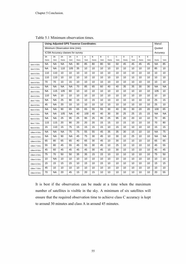
Chapter 5 Conclusion.
Table 5.1 Minimum observation times. Using Adjusted GPS Traverse Coordinates: Manuf.
Minimum Observation time (min). Quoted
ICSM Accuracy classes for survey Accuracy
3A
Horiz.
3A
Vert.
2A
Horiz.
2A
Vert.
A
Horz.
A
Vert.
B
Horiz.
B
Vert.
C
Horiz.
C
Vert.
D
Horiz.
D
Vert.
E
Horiz.
E
Vert. Horiz. Vert.
1km 4 SVs NA NA NA NA 90 85 80 80 50 50 45 45 45 45 NA 85
1km 5 SVs NA NA 110 105 35 10 10 10 10 10 10 10 10 10 85 10
1km 6 SVs 110 110 10 10 10 10 10 10 10 10 10 10 10 10 10 10
1km 7 SVs 110 110 10 10 10 10 10 10 10 10 10 10 10 10 10 10
1km 8 SVs 70 70 10 15 10 10 10 10 10 10 10 10 10 10 10 10
2km 4 SVs NA NA NA NA 70 85 65 60 40 40 35 35 30 30 NA NA
2km 5 SVs NA 115 105 60 10 10 10 10 10 10 10 10 10 10 105 10
2km 6 SVs 110 NA 10 10 10 10 10 10 10 10 10 10 10 10 10 10
2km 7 SVs NA NA 25 90 15 10 15 10 10 10 10 10 10 10 25 15
2km 8 SVs 45 NA 20 10 10 10 10 10 10 10 10 10 10 10 25 10
5km 4 SVs NA NA 90 65 65 65 55 55 30 40 30 30 20 20 100 65
5km 5 SVs NA NA 105 NA 40 100 40 40 30 30 25 25 15 15 NA NA
5km 6 SVs NA NA 25 95 25 95 25 95 25 95 20 20 10 10 70 85
5km 7 SVs 115 115 20 90 20 20 20 15 15 10 15 10 10 10 70 80
5km 8 SVs 15 110 15 75 15 15 15 15 10 15 10 10 10 10 15 15
10km 4 SVs NA NA NA 75 75 55 55 45 35 35 30 15 10 10 NA 75
10km 5 SVs NA NA 90 NA 45 75 30 45 10 30 10 25 10 10 NA NA
10km 6 SVs 65 80 65 65 40 65 30 45 10 30 10 10 10 10 65 65
10km 7 SVs 55 80 45 55 45 55 30 45 10 25 10 10 10 10 45 55
10km 8 SVs 45 60 45 45 45 45 30 45 10 30 10 10 10 10 45 45
15km 4 SVs 75 70 50 50 35 35 15 15 10 10 10 10 10 10 75 50
15km 5 SVs 10 NA 10 10 10 10 10 10 10 10 10 10 10 10 10 10
15km 6 SVs 15 15 15 15 10 15 10 15 10 10 10 10 10 10 15 15
15km 7 SVs 45 10 10 10 10 10 10 10 10 10 10 10 10 10 10 10
15km 8 SVs 70 NA 20 45 15 20 15 10 10 10 10 10 10 10 20 55
It is best if the observation can be made at a time when the maximum
number of satellites is visible in the sky. A minimum of six satellites will
ensure that the required observation time to achieve class C accuracy is kept
to around 30 minutes and class A in around 45 minutes.
55
Chapter 5 Conclusion.
5.4 Limitations.
This study is subject to some limitations that may have some bearing on the
results.
The first of these is that the permanent survey marks only carry 3rd order
coordinates and can only be used to analyse for class C accuracy in the
observed results. The use of adjusted coordinates is not an ideal solution as
they are based on the very observations that are being analysed. This was
only deemed appropriate as the closure of the traverse loop was suitably
accurate. The assumption being made is that, if the loop closure is accurate
within ICSM class 2A constraints then the individual baselines should be of
similar accuracy.
The omission of the zero baseline test from the study due to hardware
unavailability places some doubt on whether or not the two receivers
perform identically. The accuracy of the end results, particularly the
comparison of the shorter baselines against the known permanent mark
coordinates, show that the receivers are operating correctly.
The locations of the permanent marks were chosen to achieve the necessary
differences in baseline length as well as their view of the sky. To achieve a
reasonable view of the sky in the Bendigo area means using marks placed
within road reserves, this means that almost all of the marks used were
under or near overhead power lines. There were also some trees close to
marks PM872 (to the south) and PM56 (to the east). The observations still
represent real world surveying conditions and, as the end accuracy exceeds
the manufacturer’s claims, it is assumed that the trees had little effect on this
evaluation.
56
Chapter 5 Conclusion.
In an ideal test network the baselines will be of varied length but also in
varied directions. The marks used in this study allowed baselines in a
predominantly north-east to south-west direction. This is due to the lack of
suitable marks further to the east and west of the main highway and railway
through the centre of the city.
5.5 Further Work.
It was hoped to evaluate results produced using both broadcast and precise
ephemerides in this project. A software issue prevented this comparison
being conducted in time. The effect of using the downloaded precise data
may be examined in the future.
This project has analysed the performance of the Ashtech ProMark2 GPS
survey system in static survey mode only. The equipment is also capable of
measuring points in both stop and go (rapid static) and kinematic modes.
These procedures have not been analysed in this work and represent a future
possibility for exploration.
5.6 Conclusion.
The Ashtech ProMark2 GPS survey system has been shown to perform as
claimed by the manufacturer. It is suitable for applications in cadastral,
engineering and even geodetic surveying.
57

Chapter 5 Conclusion.
The analysis of the results from this project has allowed some
recommendations on observation duration to be made depending on the
satellite availability and the length of the baseline to be observed (see table
5.1).
Though the work is based on some limiting factors and assumptions the
results obtained provide a realistic and representative evaluation of the
equipment in question.
58

List of References.
LIST OF REFERENCES
Martin 2003, GPS Basics: Around and Around with Orbits, Professional
Surveyor Magazine, volume 23, number 6, viewed 23 April 2006,
<http://www.profsurv.com/archive.php?issue=77&article=1083>
Natural Resources 2003, Information Management Toolkit, section 10.2,
Best practice guidelines for GPS surveys, Commonwealth of Australia,
viewed 23 April 2006, <http://www.nlwra.gov.au/archive/toolkit/10/10-
2.html#1022>
ISCM 2004, Standards and Practices for Control Surveys, Inter-
Governmental Committee on Surveying and Mapping, version 1.6, viewed
23 April 2006,
<http://icsm.gov.au/icsm/publications/sp1/sp1v1-6.pdf>
Pace et al 1995, The Global Positioning System Assessing National Policies,
RAND, Washington.
Survey Board 2006, Practice Handbook, part 2, section 12, Guidelines for
Cadastral Surveying using Global Navigation Satellite Systems (GNSS),
Victoria.
SMES 2006, Locate Survey Marks, Victorian State Government, viewed 4
May 2006,
<http://www.services.land.vic.gov.au/landchannel/content/surveymarkintrod
uction>
59
List of References.
SNAP-UNSW 1999a, Satellite Navigation And Positioning lab, University
of New South Wales, viewed 6 September 2006,
<http://www.gmat.unsw.edu/snap/gps/gps_survey/chap4/443.htm>
SNAP-UNSW 1999b, Satellite Navigation And Positioning lab, University
of New South Wales, viewed 6 September 2006,
<http://www.gmat.unsw.edu/snap/gps/gps_survey/chap4/441.htm>
SNAP-UNSW 1999c, Satellite Navigation And Positioning lab, University
of New South Wales, viewed 6 September 2006,
<http://www.gmat.unsw.edu/snap/gps/gps_survey/chap2/222sats.htm>
Surveying Regulation 2001 (New South Wales).
Surveyors (Cadastral Surveying) Regulations 1995 (Victoria).
Surveyors Regulation 1992 (Queensland).
USACE 2003, NAVSTAR Global Positioning System Surveying, United
States Army Corps of Engineers, viewed 26 March 2006,
<http://www.usace.army.mil/usace-docs/eng-manuals/em1110-1-1003/c-
9.pdf>
Vicmap Property 2006, Digital Cadastre maps, Victorian State Government,
Victoria.
60

Appendix A Project Specification.
APPENDIX A
PROJECT SPECIFICATION
61

Appendix A Project Specification.
University of Southern Queensland
Faculty of Engineering and Surveying
ENG4111/4112 Research Project PROJECT SPECIFICATION
FOR: Neil Geoffrey SHAW TOPIC: Evaluation of Ashtech ProMark 2 survey system. SUPERVISOR: Mr. Glenn Campbell. PROJECT AIM: This project aims to evaluate the performance of the
Ashtech ProMark 2 GPS survey system in static mode.
PROGRAMME: Issue A, 9th March 2004 1. Select PSMs for different length baseline measurements. 2. Measure baselines on consecutive days at the same time each day. 3. Process results for each baseline varying the observation time and
number of satellites (and hence DOPs). 4. Analyse the results to determine the accuracy for each of the different
baseline lengths, observation times, number of satellites and DOPs. 5. Repeat analysis using downloaded precise ephemerides. 6. Compare accuracy of results for each of the different variables (baseline
length, observation time, number of satellites, DOPs and broadcast or precise ephemerides).
7. Draw conclusions as to the required observation times for given baseline
lengths and number of satellites. AGREED: _____________(student) ____________(Supervisor) ____/____/____ ____/____/____
62

Appendix B Accuracy standards.
APPENDIX B
ACCURACY STANDARDS
63
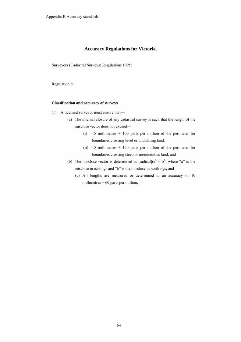
Appendix B Accuracy standards.
Accuracy Regulations for Victoria.
Surveyors (Cadastral Surveys) Regulations 1995:
Regulation 6:
Classification and accuracy of surveys
(1) A licensed surveyor must ensure that—
(a) The internal closure of any cadastral survey is such that the length of the
misclose vector does not exceed—
(i) 15 millimetres + 100 parts per million of the perimeter for
boundaries crossing level or undulating land.
(ii) 15 millimetres + 150 parts per million of the perimeter for
boundaries crossing steep or mountainous land; and
(b) The misclose vector is determined as [radical](a2 + b2) where “a” is the
misclose in eastings and “b” is the misclose in northings; and
(c) All lengths are measured or determined to an accuracy of 10
millimetres + 60 parts per million.
64
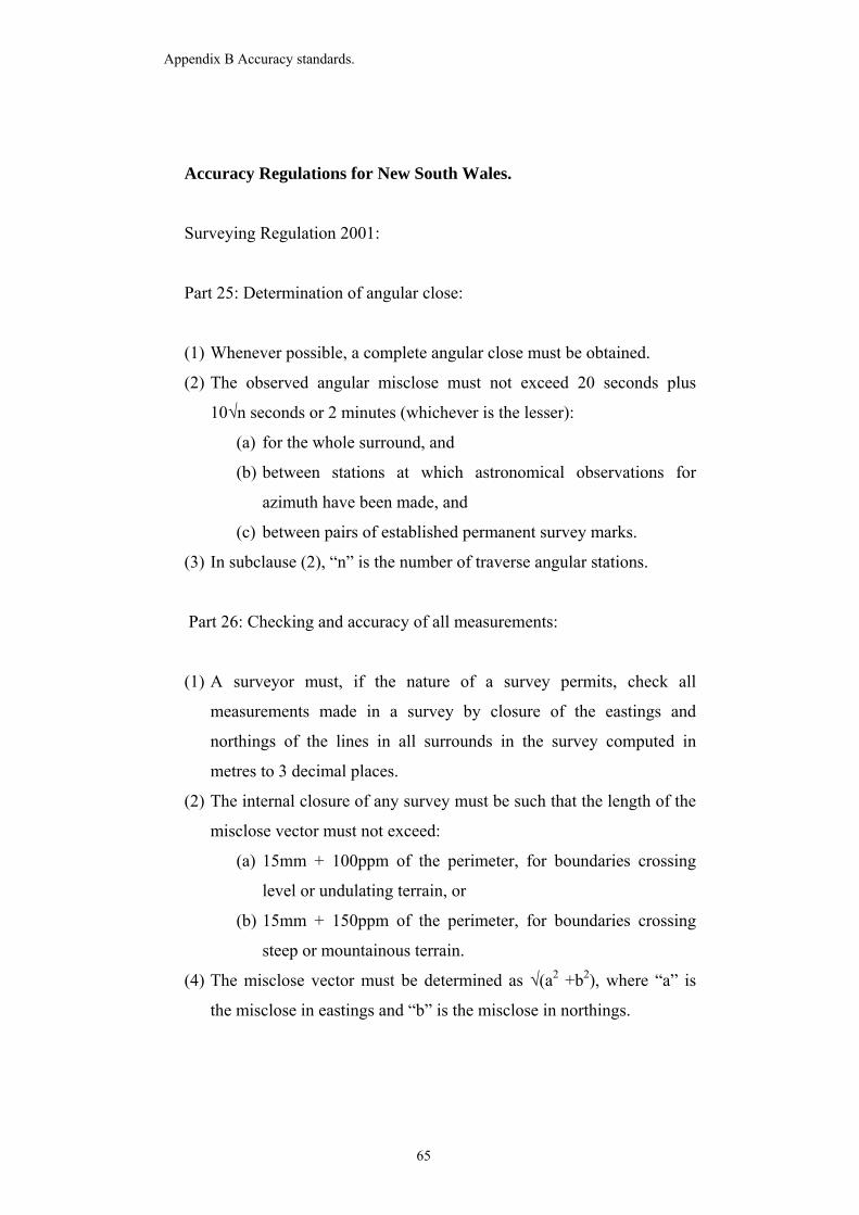
Appendix B Accuracy standards.
Accuracy Regulations for New South Wales.
Surveying Regulation 2001:
Part 25: Determination of angular close:
(1) Whenever possible, a complete angular close must be obtained.
(2) The observed angular misclose must not exceed 20 seconds plus
10√n seconds or 2 minutes (whichever is the lesser):
(a) for the whole surround, and
(b) between stations at which astronomical observations for
azimuth have been made, and
(c) between pairs of established permanent survey marks.
(3) In subclause (2), “n” is the number of traverse angular stations.
Part 26: Checking and accuracy of all measurements:
(1) A surveyor must, if the nature of a survey permits, check all
measurements made in a survey by closure of the eastings and
northings of the lines in all surrounds in the survey computed in
metres to 3 decimal places.
(2) The internal closure of any survey must be such that the length of the
misclose vector must not exceed:
(a) 15mm + 100ppm of the perimeter, for boundaries crossing
level or undulating terrain, or
(b) 15mm + 150ppm of the perimeter, for boundaries crossing
steep or mountainous terrain.
(4) The misclose vector must be determined as √(a2 +b2), where “a” is
the misclose in eastings and “b” is the misclose in northings.
65
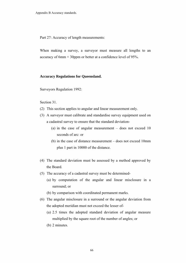
Appendix B Accuracy standards.
Part 27: Accuracy of length measurements:
When making a survey, a surveyor must measure all lengths to an
accuracy of 6mm + 30ppm or better at a confidence level of 95%.
Accuracy Regulations for Queensland.
Surveyors Regulation 1992:
Section 31.
(2) This section applies to angular and linear measurement only.
(3) A surveyor must calibrate and standardise survey equipment used on
a cadastral survey to ensure that the standard deviation-
(a) in the case of angular measurement – does not exceed 10
seconds of arc: or
(b) in the case of distance measurement – does not exceed 10mm
plus 1 part in 10000 of the distance.
(4) The standard deviation must be assessed by a method approved by
the Board.
(5) The accuracy of a cadastral survey must be determined-
(a) by computation of the angular and linear misclosure in a
surround; or
(b) by comparison with coordinated permanent marks.
(6) The angular misclosure in a surround or the angular deviation from
the adopted meridian must not exceed the lesser of-
(a) 2.5 times the adopted standard deviation of angular measure
multiplied by the square root of the number of angles; or
(b) 2 minutes.
66
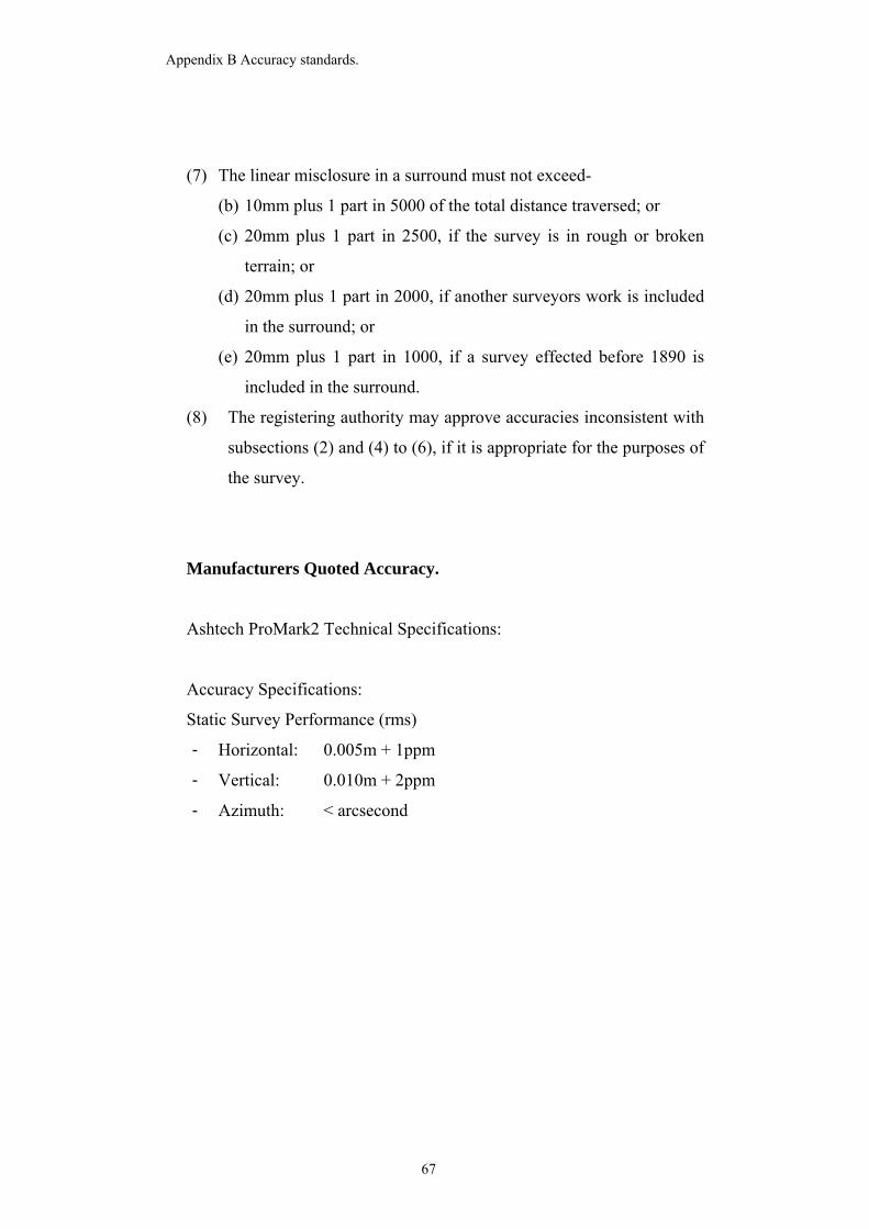
Appendix B Accuracy standards.
(7) The linear misclosure in a surround must not exceed-
(b) 10mm plus 1 part in 5000 of the total distance traversed; or
(c) 20mm plus 1 part in 2500, if the survey is in rough or broken
terrain; or
(d) 20mm plus 1 part in 2000, if another surveyors work is included
in the surround; or
(e) 20mm plus 1 part in 1000, if a survey effected before 1890 is
included in the surround.
(8) The registering authority may approve accuracies inconsistent with
subsections (2) and (4) to (6), if it is appropriate for the purposes of
the survey.
Manufacturers Quoted Accuracy.
Ashtech ProMark2 Technical Specifications:
Accuracy Specifications:
Static Survey Performance (rms)
- Horizontal: 0.005m + 1ppm
- Vertical: 0.010m + 2ppm
- Azimuth: < arcsecond
67
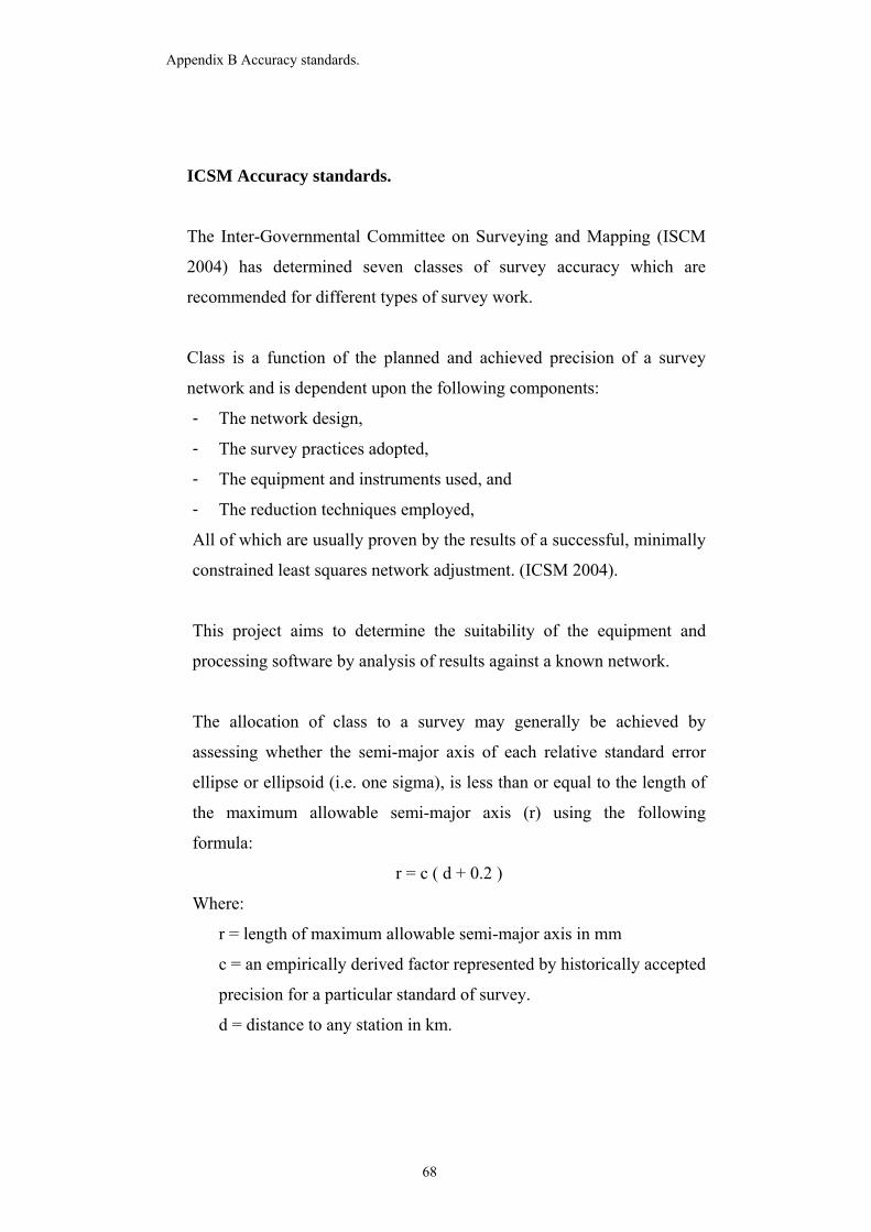
Appendix B Accuracy standards.
ICSM Accuracy standards.
The Inter-Governmental Committee on Surveying and Mapping (ISCM
2004) has determined seven classes of survey accuracy which are
recommended for different types of survey work.
Class is a function of the planned and achieved precision of a survey
network and is dependent upon the following components:
- The network design,
- The survey practices adopted,
- The equipment and instruments used, and
- The reduction techniques employed,
All of which are usually proven by the results of a successful, minimally
constrained least squares network adjustment. (ICSM 2004).
This project aims to determine the suitability of the equipment and
processing software by analysis of results against a known network.
The allocation of class to a survey may generally be achieved by
assessing whether the semi-major axis of each relative standard error
ellipse or ellipsoid (i.e. one sigma), is less than or equal to the length of
the maximum allowable semi-major axis (r) using the following
formula:
r = c ( d + 0.2 )
Where:
r = length of maximum allowable semi-major axis in mm
c = an empirically derived factor represented by historically accepted
precision for a particular standard of survey.
d = distance to any station in km.
68
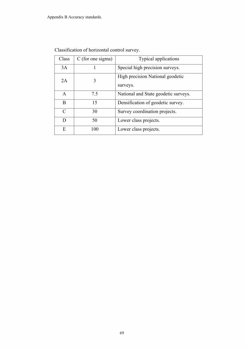
Appendix B Accuracy standards.
Classification of horizontal control survey.
Class C (for one sigma) Typical applications
3A 1 Special high precision surveys.
2A 3 High precision National geodetic
surveys.
A 7.5 National and State geodetic surveys.
B 15 Densification of geodetic survey.
C 30 Survey coordination projects.
D 50 Lower class projects.
E 100 Lower class projects.
69

Appendix C Locality Map.
APPENDIX C
LOCALITY MAP
70
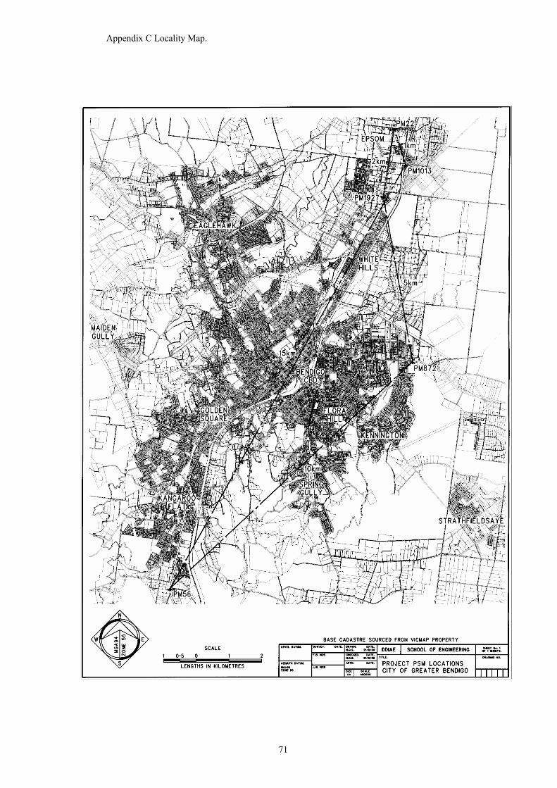
Appendix C Locality Map.
71

Appendix D Permanent Survey Mark Sketch Plans.
APPENDIX D
PERMANENT SURVEY MARK
SKETCH PLANS
72
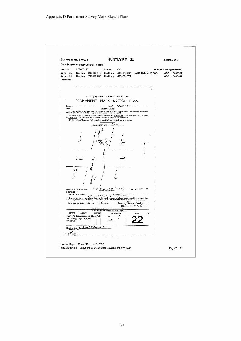
Appendix D Permanent Survey Mark Sketch Plans.
73
Appendix D Permanent Survey Mark Sketch Plans.
74
Appendix D Permanent Survey Mark Sketch Plans.
75
Appendix D Permanent Survey Mark Sketch Plans.
76
Appendix D Permanent Survey Mark Sketch Plans.
77