How Well do Individuals Predict the Selling Prices of their Homes?

by Hugo Benítez-Silva*, Selcuk Eren**

Frank Heiland*** and Sergi Jiménez-Martín****

DOCUMENTO DE TRABAJO 2008-10

Serie Nuevos Consumidores CÁTEDRA Fedea – BBVA

Serie Economía de la Salud y Hábitos de Vida

CÁTEDRA Fedea – “la Caixa”

February 2008

* SUNY-Stony Brook, IAE-CSIC, and FEDEA ** Hamilton College*** Florida State University ** Universitat Pompeu Fabra, and FEDEA Los Documentos de Trabajo se distribuyen gratuitamente a las Universidades e Instituciones de Investigación que lo solicitan. No obstante están disponibles en texto completo a través de Internet: http://www.fedea.es. These Working Paper are distributed free of charge to University Department and other Research Centres. They are also available through Internet: http://www.fedea.es. ISSN:1696-750X

How Well do Individuals Predict the Selling Prices of their Homes?†

Hugo Benítez-Silva

SUNY-Stony Brook, IAE-CSIC, and FEDEA

Selcuk Eren Hamilton College

Frank Heiland

Florida State University

Sergi Jiménez-Martín Universitat Pompeu Fabra, and FEDEA

April 28, 2008

Abstract

Self-reported home values are widely used as a measure of housing wealth by researchers employing a variety of data sets and studying a number of different individual and household level decisions. The accuracy of this measure is an open empirical question, and requires some type of market assessment of the values reported. In this research, we study the predictive power of self-reported housing wealth when estimating sales prices utilizing the Health and Retirement Study. We find that homeowners, on average, overestimate the value of their properties by between 5% and 10%. More importantly, we are the first to document a strong correlation between accuracy and the economic conditions at the time of the purchase of the property (measured by the prevalent interest rate, the growth of household income, and the growth of median housing prices). While most individuals overestimate the value of their properties, those who bought during more difficult economic times tend to be more accurate, and in some cases even underestimate the value of their house. These results establish a surprisingly strong, likely permanent, and in many cases long-lived, effect of the initial conditions surrounding the purchases of properties, on how individuals value them. This cyclicality of the overestimation of house prices can provide some explanations for the difficulties currently faced by many homeowners, who were expecting large appreciations in home value to rescue them in case of increases in interest rates which could jeopardize their ability to live up to their financial commitments. Keywords: Self-Reported Housing Values, Housing Prices, Instrumental Variables, Sample Selection, Business Cycle, Interest Rates, Health and Retirement Study JEL classification: E21, C33, C34 † Benítez-Silva acknowledges the financial support from Grant Number 5 P01 AG022481-04 from the National Institute on Aging on a related project, and along with Heiland they thank the MRRC for their support on a related project. Jiménez-Martín acknowledges the financial support of the Spanish Ministry of Education through project number SEJ2005-08783-C04-01. Any remaining errors are the authors’.

1. Introduction and Motivation

Housing wealth is one of the pillars of the well-being of Americans families, especially because

it represents more than 60% of the average net wealth of US households, according to the

Federal Reserve's 2004 Survey of Consumer Finances (SCF).1 While the current tumultuous

times in the housing market seem to indicate the presence of possibly serious errors in predicting

the evolution of housing prices and mortgage rates by a non-trivial proportion of home owners,

we know relatively little about the ability of households to predict the market value of their

homes in the context of household level representative surveys and using data on sales prices of

those properties. While a number of researchers have described the existence of some

overestimation in housing values (in the 3% to 6% range in the last studies), as far as we know,

we are the first researchers to analyze the predictive power of self-reported housing wealth in an

econometric model of sales prices.2

Understanding the accuracy of self-reported housing wealth is of great importance in a

variety of contexts, since it is a pervasive explanatory variable (either by itself or as a component

of net individual or household worth) in just about any empirical analysis or behavioral model of

individuals’ and households’ decision making. For example, it is a key variable in decisions such

as retirement (see e.g., Moore and Mitchell 2000, Engen, Gale, and Uccelo 1999 and 2005,

Gustman and Steinmeier 1999, and Lusardi and Mitchell 2007), consumption (Skinner 1989,

Case, Quigley, and Shiller 2005, Tang 2006, and Agarwal 2007), and savings (Hoynes and 1 See Bucks, Kennickell, and Moore (2006). This fraction is considerably lower than in some European Countries. For example, in Spain housing wealth represents 87.5 % of net wealth. 2 Most studies use the American Housing Survey, which follows houses rather than households, or the Survey of Consumer Finances (SCF), which is not a panel data survey. See Agarwal (2007), Kiel and Zabel (1999), and Goodman and Ittner (1992). The first study on this issue was published by Kish and Lansing (1954) using the 1950 SCF, and it was not until Kain and Quigley (1972) that this was revisited. The latter authors acknowledge that “the only accurate estimate of the value of a house is its sale price…”, however, due to data limitations, and what they perceived as possibly serious selection problems, their analysis focused, as the early study, on comparisons of households’ self-reports with appraisals by experts. The latter can be considered indirect market assessments, since they use information on similar properties, and try to control for the observable characteristics of the property.

2

McFadden 1997, Klyev and Mills 2006 and Juster, Lupton, Smith, and Stafford 2005). However,

since in household surveys housing wealth is typically self-reported, it is likely to be exposed to

measurement error, and its accuracy has not been studied in much detail.3

In this research, we take a closer look at the accuracy of self-reported housing wealth,

using the Health and Retirement Study (HRS), in particular a rarely used section on capital gains,

where sales prices are reported by homeowners. This allows us to compare the self-reported

housing values with self-reported sale prices. In particular, it enables us to estimate a sales price

equation as a function of self-reported housing wealth in the previous interview of the panel

study.4 We find, using OLS regressions, sample selection corrected specifications to control for

the possible bias in the ownership decision, and Instrumental Variables specifications to account

for the measurement error problem, that homeowners on average overestimate the value of their

properties by between 5% and 10%. We also show that the overestimation is primarily due to the

large expected capital gains implicit in the self-reported home values, especially since the mid

1980s.

There is, however, considerable variation in how accurately homeowners predict the

value of their properties depending on when individuals bought their homes. While most

individuals overestimate the value of their homes (some by as much as 20%), individuals who

acquire their properties during economic downturns tend to be more accurate, and in some cases

even underestimate the value of their houses.

3 This measurement error and the attenuation bias that goes with it, can explain that wealth measures in general, and housing wealth in particular, are, in a number of empirical settings, found not to have a lot of predictive power (see Venti and Wise (2001), Juster, Lupton, Smith, and Stafford (2005), and Tang (2006)). 4 Sales prices do not always reflect market values due to the existence of many complex transactions that include, for example, personal property, land exchanges, and within family sales. This also means that the terms of the sale could vary over the business cycle. Unfortunately, we cannot assess the importance of these issues with our data. However, it is not obvious whether in the presence of some or all of these in any data on selling prices, the reported values will be systematically higher or lower than the market values.

3

We document a strong correlation between the evolution of our accuracy estimates over

time, and the business cycle. In periods of high interest rates and declining incomes, the buyers

are likely to have lower appreciation expectations due to the declining housing prices, and end up

assessing, on average, more accurately the value of their homes, and even in some cases

underestimating it. Furthermore, the buyers during the downturns tend to be more educated

which is likely to be correlated with having better information about the value of their homes.

These results establish a surprisingly strong, likely permanent, and in many cases long-lived

effect of the initial conditions surrounding the purchases of properties, on how individuals value

them.

Our results provide some explanations for the difficult situation that many homeowners

are currently facing, since they are consistent with the growing evidence of the existence of a

sizable fraction of home owners (many of them first time buyers, given the increasing home-

ownership rates in the period) who bought their houses in the last decade with soft (and risky)

mortgages, expecting large appreciations in home value to rescue them in case of increases in

interest rates which could jeopardize their ability to live up to their financial commitments.

In Section 2, we propose a simple method for testing the accuracy of self-reported

housing wealth and introduce some natural instruments to control for measurement error in this

type of models, in the presence of possible sample selection bias concerns. We present our data

and summary statistics in Section 3. The main empirical results are presented and discussed in

Section 4, and Section 5 analyzes the relationship between our accuracy estimates and the

business cycle. Section 6 provides some conclusions.

4

2. Testing the Accuracy of Self-Reported Housing Values using Sales Prices

Suppose that tiy represents the actual market value of the homeowner i 's house at time t and

is the self-reported house value at a point in time before the sale. A simple model to test the

accuracy of the reported home value can be written as:

1tiX −

1t ti iy X iβ ε−= + (1)

If the homeowners predict the market value of their house accurately, we expect to find

that . If homeowners overestimate (underestimate) the value of their home, then

the estimated slope coefficient

[ | , ] 1it

i iE Xβ ε =

β will be less than (more than) one.5 Estimating (1) is in principle

straightforward through a simple conditional moment estimator like Ordinary Least Squares,

but the likely presence of unobserved heterogeneity (which could be reflected in the presence of

measurement error in the variables of interest), which raises endogeneity concerns, and a

potential sample selection bias concern (given that only a relatively small proportion of

individuals sell their houses during the period of analysis) complicate the identification. We use

three alternative specifications in order to address these issues.

2.1 OLS Specification

In the data we observe the market value of a property when the individual reports,

retrospectively, the price at the time of the sale of a house they owned in the last survey wave.

Therefore, the self-reported house value is obtained from the previous wave of data. Given data

collection every other year only, there may be as many as 24 months between the measurement

of the sale price and the self-reported house value. In the interview, individuals are asked about 5 There is no reason to believe that the model should contain a constant as there is no minimum market value for the houses, and the left and right hand side are measuring the same asset. In fact, we have run several empirical specifications with a constant and it comes out to be insignificant, as expected, no matter how we specify the model. In the empirical work we present results with and without a constant in the regression.

5

the current market value of their homes rather than to forecast the price for some future period.

In order to correct a possible bias in the estimation of the coefficient of interest in (1) resulting

from possible appreciation (depreciation) of the value of the house during that time, we control

for the number of months between the observances of these two variables.6 The OLS

specification can then be written as follows:

1t ti iy X T iβ α− ε= + + (2)

where represents the self-reported house value from the previous wave, and T represents

the number of months between the time the market price refers to and the self-reported home

value.

1tiX −

2.2 IV Specification

As with all survey data, measurement error in the variables of interest is a major concern. We are

particularly interested in accounting for potentially noisy self-reports of the house values, and

reporting errors that may be correlated with measurement errors in other factors or omitted

variables. For example, it is natural to expect a degree of inaccuracy in estimating the effect of

home improvements and updates done to the property over the years on the value of the house.

6 Notice, that this discrepancy in the timing of the assessment suggests that the relationship in (1) is potentially non-linear. We have allowed for the difference in months to enter non-linearly (which could capture changing economic conditions in the months before the sale which could affect the price, like movements in the interest rates), but results have not changed. One possible alternative would be to adjust all the observed prices to the same time period. This, however, may create some unwanted measurement error since in many cases there were only a few months of difference between reports. Also, the only location information in the public releases of the HRS is the region of the residence, so the best we can do is to adjust for the region level house price index. There is a lot of variation in the change in the house prices even within the same county and such a crude adjustment will only provide more measurement error to the variable. More importantly there is no reason to believe that the house values should keep up with the inflation rate. Nevertheless, we used several ways of adjusting for inflation in addition to simply controlling for time differences. These results were consistent with those reported in the present paper. Additionally, due to the fact that it might be natural to expect β to be higher where there is less of a lag, which suggests T should be interacted with the owner's estimate, we have performed an extensive sensitivity analysis of the consequences of including this interaction term. The results of our preferred specification remain literally unchanged, therefore, the empirical evidence suggest that those who sell shortly after the interview do not report systematically more accurate estimates of the selling price of their properties than those who sell shortly before the following interview.

6

This component of self-reports could lead to a significant bias in the coefficient of interest. In

order to eliminate this bias, we need to capture the true component of the reported home value.

To do so we propose an Instrumental Variables (IV) approach. If measurement error was not a

problem we would expect the β coefficient of the IV estimator to be very close to the one from

the OLS specification, assuming validity of the instrument set.

The longitudinal structure of our data readily provides us with a candidate for an

instrument. Homeowners repeat their house values in consecutive periods. It is natural to

conjecture that past self-reported house values are correlated with the recent self-reported house

value variable, but are uncorrelated with the disturbances in the actual sale price equation.7 We

can formally state this IV specification as follows:

10 1

t ti iX Xδ δ− −2

ie= + + (3)

1ˆt ti iy X T iβ α−= + +ε (4)

where 1ˆ tiX − represents the predicted values from equation (3). In the empirical analysis, and in

order to test the properties of the exclusion restrictions, we also use as instrument the tenure on

the house (that is, the duration of ownership on the house), since it does not show much

correlation with the selling price. As we discuss below, both instruments pass the conventional

exogeneity test (over-identification test) presented in the literature.

Another possible natural exclusion restriction, with likely better theoretical properties, is

the difference between , the twice lagged self-reported value of housing, and , the three

times lagged self-reported value of housing, since it basically eliminates the possibility of any

2tiX − 3t

iX −

7 The use of lagged endogenous variables as possible exclusion restrictions in IV estimations has a fairly long tradition (Hansen and Singleton (1983), Hall (1988), and Patterson and Pesaran (1992)), but it frequently encounters the problem of weak instruments (Yogo (2004)). In our case, however, the self-reported house value follows a highly autoregressive process allowing us to strongly reject that we have weak instruments.

7

correlation with the person specific component that might be present in the error term in the

equation of interest. We have estimated such a model, and while the point estimate of β is

slightly lower, the lack of efficiency (due to the fact that this instrument is not as strong as the

level of the twice lagged self-reported home value), which results in much larger standard errors,

the loss of another 175 observations, and the (good) results of the over-identification tests of the

previous specification, convinces us that the main IV specification we should use come from the

one discussed above. We discuss the results using this alternative instrument set in section 4.

2.3 IV with Selection

Given that we observe only for the homeowners who sell their houses, and only a relatively

small portion of homeowners sell in any given survey wave, we are concerned with selection on

unobservables; namely, homeowners who sell their houses may be different from homeowners

who do not sell their houses in some unobserved characteristics. If that is the case, the estimated

coefficients from OLS and IV may be biased. For example, if homeowners who sell their houses

are more knowledgeable about the overall market, their home value estimates would be more

accurate and β coefficients estimated using OLS or IV would be biased towards one.

tiy

However, the selection process here is non-standard, in the sense that individuals have

many chances to sell their homes during the survey period, but only do it once. Econometrically

that means that we observe a given individual over time making the selling decision repeatedly

(mostly choosing not to sell), while we only observe one instance of sale. That means that the

selection equation has both a time-invariant individual specific component and a time variant

idiosyncratic error term.

In order to purge our OLS or IV estimates of the possible biases resulting from this

selection mechanism, we follow a two-step procedure described in Wooldridge (1995), and also

8

in line with the discussion in Hsiao (1986), which without needing the distributional assumptions

discussed for example in Jensen, Rosholm, and Verner (2001), provides a consistent (but likely

inefficient) estimation procedure.8

The corresponding IV approach with selection is as follows:

1 1, ,1( 0)t t

i t i i i i tZ a bHE cX u κ− −= + + + + > (5)

10 1

t ti iX Xδ δ− −= + +2

ie

iv

(6)

1ˆt ti i iy X Tβ α λπ−= + + + (7)

where equation (5) is a period by period probit estimate of the selling decision, which allows, as

discussed by Wooldridge (1995), to account for the likely serial correlation between the selling

decisions over time by a given individual. The selling decision depends on home equity at the

time of the sale ( ), and the expected home value (1tiHE − 1t

iX − ). Home equity is a natural choice

for the exclusion restriction, since on theoretical grounds it should not affect the selling price

(and empirically, we do not find evidence to suggest otherwise), and it seems to perform as a

summary statistic for a large number of household characteristics and initial conditions such that

is highly correlated with the selling decision.9 From the period by period probit estimates, we

8 Our case fits the one described in sections 3.2 and 4.2 in Wooldridge (1995). Baltagi (2005) also describes this sample selection bias correction procedure. 9 Technically we do not need the exclusion restriction to identify this model given the non-linearity resulting from the distributional assumption (normality) of the error term in equation (5), but we follow the conventional practice of including at least one likely exogenous variable to provide non-parametric identification to the model. We have also experimented with a different estimation strategy, following Olsen (1980), in which the selection equation is modeled as a Linear Probability Model, and after an error transformation a correction term is constructed in the spirit of Heckman (1979). The advantage of this technique is that we can easily account for the error structure that includes the individual component and the idiosyncratic component, and we can experiment with the inclusion of larger number of exogenous variables in the selection equation which were more problematic to include in the non-linear first stage due to their likely endogeneity, which here can be more easily overcome with IV techniques. Similarly to Olsen (1980) we find essentially identical results using both methods, and since in both cases selection matters very little to our results, we have chosen to present the results of the more traditional selection correction specifications. The results using the alternative specification are available from the authors upon request.

9

construct an inverse mills ratio ( iλ ) that is used to control for the selection in the main equation

(7).10

The uncorrected and corrected IV estimates are obtained from estimating the system

using GMM, correcting the standard errors for unknown forms of heteroskedasticity, and using

the optimal weighting matrix to obtain consistent and efficient estimates, even in the presence of

arbitrary serial correlation of the disturbances.11

3. The Health and Retirement Study: Self-Reports on House Values and

Selling Prices

While the HRS is the data set of choice when analyzing retirement behavior, the savings, the

health status of older Americans, etc., given its wealth of demographic, health, and socio-

economic data, as well as detailed assets and income sections, it has been rarely used to analyze

questions regarding the housing market. However, a rarely used section of the HRS provides

very detailed information about real estate transactions by households, which allow us to

repeatedly observe self-reported house values, as well as the selling prices of properties sold in

the 1994 to 2002 period, using the first six waves of the HRS. The HRS is a nationally

representative longitudinal survey of 7,700 households headed by an individual aged 51 to 61 as

of the first interviews in 1992-93. The sixth round of data was collected in 2002.

In this analysis, we include respondents who are financially knowledgeable members of

the household who own a house and report the value of their house(s). We restrict our analysis to

the first home only, since the second home information is rather incomplete and difficult to 10 Jiménez-Martín (2006), and Jiménez-Martín and García (2007) use this specification in their panel data models of wage bargaining, and Benítez-Silva and Dwyer (2005), and Benítez-Silva et al. (2007) discuss related models using a similar type of specification. 11 In the implementation of this procedure we have followed the practical suggestions in Baum, Schaffer, and Stillman (2003 and 2007).

10

match when the transaction involves the second home.12 In each wave respondents are asked

whether they own a house and to assess the market value of their house if it were to be sold at

that point in time. In a different section, individuals are asked whether any transaction occurred

since the last wave (buy or sell or both), the sale price of the house if there was a sale, and the

purchase price of the new home. The information about the purchase price and the purchase year

of a house is gathered from the heads of households in 1992. The purchase price is updated for

those who bought a house in the latter waves. We compare the self-reported house value from

period t-1 and the selling price information obtained from period t if a sale occurred between

survey waves.

Table 1 summarizes the characteristics of the financially knowledgeable homeowners and

their assets. The columns break down the sample according to the selection criteria: whether or

not individuals sell their house during the six waves, and for the sellers we divide between the

full sample of sellers and the estimation sample. Note that given the longitudinal nature of the

sample, homeowners may be observed up to six times, but are asked whether they sold a house

they owned at only five of those occasions.

The criteria used to select the estimation sample are the following: from the 1,067

observations we have in the HRS that report valid positive selling prices on their homes and at

the same time reported a valid value of a home they previously owned, we had to eliminate 204

observations because we did not have valid information about when they bought that home or

when they sold it. Not having information on the first of those variables does not allow us to

match the property exactly, and not having information on the second prevents us from using the

12 In fact, even matching the sale of the first home is rather complicated since the question used asks about transactions on a first or second home. By matching the year in which the house was bought, which is asked both in the assets section and the capital gains section, and using information on whether individuals owned a second home, we have been able to pin down the property actually sold with a high level of accuracy, which we have verified observation by observation.

11

difference in months between the time of the self-report of the value and the time they sold the

property, which is an important variable in our econometric model.

We further lose 244 observations because of a missing lagged value of the home they are

selling, which is used in the IV-GMM estimation as an exclusion restriction. Using the lagged

value of the home essentially eliminates the sales occurred between the first two waves of the

HRS (between 1992 and 1994), or sales by respondents who have not been interviewed for at

least three waves. We also lose 20 observations because of missing home equity which is used in

the probit equation in the Corrected IV-GMM specification. Finally, we also eliminate

homeowners who report a sale price 0.2 times and less, or 5 times and more, than the self-

reported house value (a total of 25 individuals). These extreme values occur mostly due to

coding errors.13

As shown in Table 1, those who did not sell a house during the period in which they are

observed, report lower home values, purchase prices, and capital gains. The average home tenure

for sellers is shorter than for non-sellers, but it is still almost 18 years. On the other hand, non-

sellers have less home equity, are less likely to be white, have lower educational attainments, and

lower earnings. The marital status, average age and gender composition are similar for both

sellers and non-sellers.

Looking at the sellers, we observe that self-reported home values are larger than selling

prices by around 2% for the full sample, but only around 0.6% larger for the estimation sample.

The estimation sample displays slightly longer tenure in the house that is eventually sold, and a

slightly greater selling price.

13 Due to all these restrictions our estimated sample is reduced to the 574 observations used in the estimations. The results using the full sample of sellers, but using OLS to avoid losing observations due to missing lagged endogenous variables, are quantitatively almost identical to those discussed in the next section. In particular, allowing for a possible selection from the full sample into the estimation sample did not have any effect on the coefficients reported in the paper.

12

4. Main Econometric Results

As discussed in Section 2, we consider three alternative estimators in order to test the accuracy

of self-reported house values. We first estimate an OLS model where we have the original house

value and the months between the report of the house value and the sale price on the right hand

side, and the sale price as the dependent variable. We control for the months between these two

reports in order to control for possible appreciation (or depreciation) in the house value as

explained in Section 2. Our preferred specification is a regression without a constant term as

there is no reason to believe that there will be a minimum sale price, and therefore a regression

through the origin is justified. However, we also present the results when including a constant

term. The latter estimates are almost identical and the constant term is not statistically

significantly different from zero.

We then estimate an IV model specification via GMM using the previous period self-

reported house value, and tenure on the house, as exclusion restrictions. Lastly, we estimate the

same model controlling for selection into selling using a period by period probit equation

approach. The selection equation contains the reported house value, household characteristics,

and home equity.

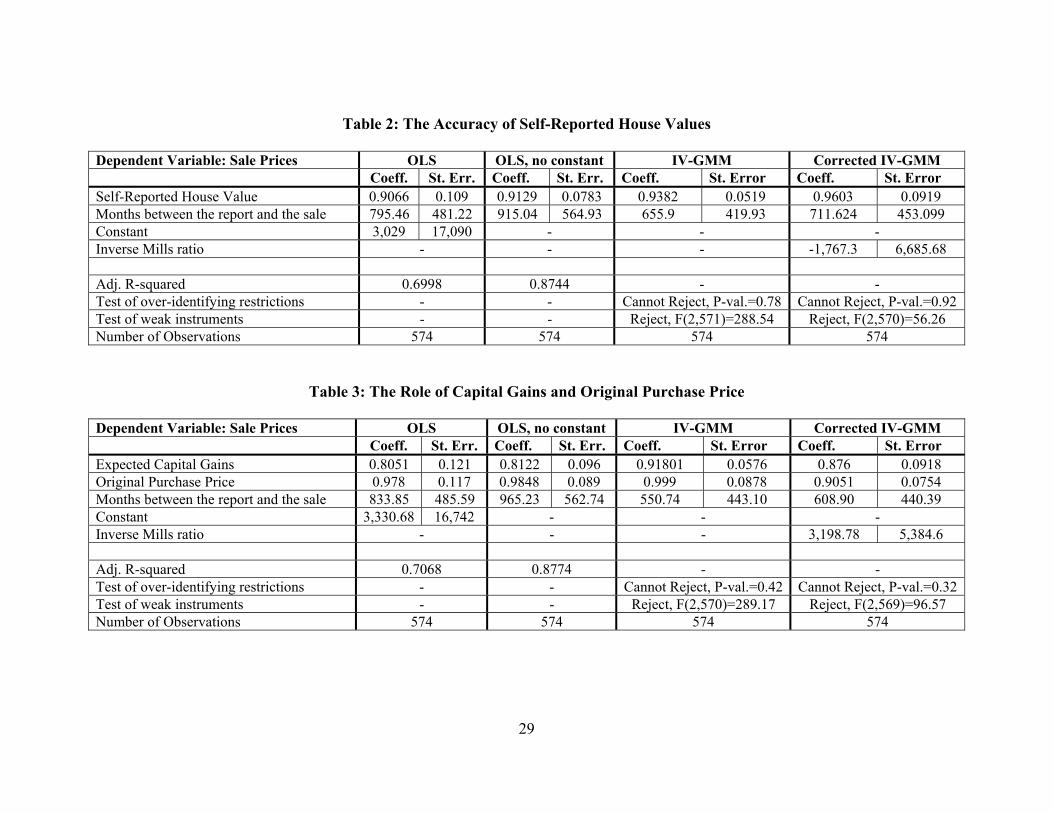
Table 2 presents the results from the different specifications and estimation strategies.

The OLS estimate of β , the coefficient on the self-reported house value, is 0.91. This point

estimate implies an overestimation of around 10% in house values.

Given the likely presence of measurement error that can lead to attenuation bias on the

coefficient of interest (i.e.β may be biased downwards), we estimate an IV specification, which

as discussed above, uses the tenure on the house and the lagged house value as exclusion

restrictions. Both the test of weak instruments and the overidentification test indicate that we

13

have valid instruments, and the fact that the standard errors actually decrease compared with the

OLS results, indicates the robustness and strength of the procedure.14 The IV results suggest a

slightly lower degree of overestimation, since β is estimated to be 0.938, implying an

overestimation of more than 6%. The coefficient is not significantly different from 1 at

conventional significant levels, but the p-value of the hypothesis that the coefficient is larger or

equal to 1 is 0.1173, which is very close to the 10% level of significance, especially taking into

account the very conservative computation of the standard errors, in order to make them robust

to heteroskedasticity and autocorrelation.15

Accounting for selection, we find the coefficient of the inverse mills ratio to be

statistically insignificant, suggesting that there is no evidence that sellers differ from non-sellers

in unobservable ways.16 While the coefficient for reported house values increases slightly, the

standard errors also increase.

In light of these results, and after performing an exogeneity test robust to violations of the

conditional homoskedasticity assumption to assess the appropriates of the IV specification versus

the OLS (see Hayashi (2000), and Baum, Schaffer, and Stillman (2007)), our preferred estimates

are the IV results, since we can reject the hypothesis that the reported home values can be taken

as exogenous to the price process.

14 We follow the suggestions in Bound, Jaeger, and Baker (1995), Staiger and Stock (1997), Stock, Wright, and Yogo (2002), and Baum, Schaffer, and Stillman (2003), and find that we have robust instruments, with very large F statistics in the first stage of the IV procedure, considerably larger than the minimum value (around 10) suggested in Staiger and Stock (1997), and also discussed in Stock, Wright, and Yogo (2002), as a good rule of thumb to check whether we are in the presence of weak instruments. Also, the model is overidentified, which allows us to test whether our instruments are exogenous with respect to the error term in the structural equation. A rejection of this test would suggest that the instruments are either not truly exogenous or they should be included in the main regression of interest. In all cases we cannot reject the overidentifying restrictions. 15 If we use as exclusion restriction the difference between the twice lagged self-reported home value and the three times lagged report, the β is estimated to be 0.898, but the standard error almost doubles from 0.051 to 0.096. At the same time the F statistic to test the strength of the instruments goes down from over 288 to just around 22. These and other sensitivity analysis results are available from the authors upon request. 16 In a related context but estimating a different type of home sale price equation, Ihlanfeldt and Martínez-Vázquez (1986) also find no evidence of sample selection bias when estimating an equation of sale prices.

14

The Role of Unrealized Capital Gains and the Original Price Paid in Assessing the Accuracy

of Housing Wealth

In this section, we investigate whether the two components of the self-reported house value, the

original price of the house and the capital gains, play different roles in predicting the market

value of a property. The measure of the unrealized capital gains is obtained by subtracting the

self-reported original purchase price from the self-reported value of the home.17

We re-estimate the models discussed above, substituting the original price and the

(unrealized) capital gains for the self-reported house value.18 In the case of completely accurate

assessment of the accumulated capital gains and original price of the house, we would expect

that both coefficients equal to one. If homeowners tend to recall the purchase price accurately but

struggle to correctly gauge the market value of the capital gains that they have accumulated in

their homes, then we may observe significant over or underestimation with respect to the

expected capital gains.19

The results are presented in Table 3. The estimates suggest that homeowners are, on

average, much less accurate with respect to their assessment of the role of capital gains for the

value of the house compared to the role of the purchase price. Specifically, the marginal effect of

17 Unrealized capital gains are inherently risky, especially when accumulated in a lumpy asset such as housing. This issue has received relatively little attention from researchers, even though some prominent policy makers, like former Chairman of the Federal Reserve Alan Greenspan (2002), emphasized the need for further disaggregation in the analysis of household portfolios, with special attention to the differential behavior implied by realized and unrealized capital gains. 18 The expected capital gains will be heavily time variant as we do not adjust for inflation and the original purchase price may rather be low. Adjusting for inflation, though, creates additional measurement error. Moreover, philosophically there is no reason to call the difference between expected price and the adjusted purchase price as capital gains since there is no reason to believe that house prices will always keep up with the inflation. Nevertheless, we specify additional models adjusting the original purchase price for inflation. The results do not differ in any significant way from the ones reported here. 19 For example, if owners base the expected rate of appreciation of their house on the reported price change of the median (or average) home purchased in their region, then they would likely end up overestimating their capital gains since the median home ages relatively less because of the renewal of the housing stock. Another source of possible over- or underestimation that would be reflected in the capital gains measure is a systematic misperception among owners of the value added by certain common updates to the house such as a new roof or a remodeled kitchen.

15

the capital gains variable is estimated to be around 0.91, indicating that homeowners may

significantly overestimate the contribution of the capital gains on the sale price. Based on our

conservative estimates of the standard errors, the p-value of the hypothesis that the coefficient is

larger or equal to 1 is 0.077, giving us statistical confidence in our point estimate of the effect of

the capital gains.

On the contrary, the original purchase price is reflected almost one to one in the selling

price; the corresponding coefficient is estimated to be 0.999. This result is consistent with the

idea that homeowners accurately recall the original purchase price but tend to overestimate the

capital gains that they have accumulated in their homes.

The latter result suggests a possible role for business cycle effects on the accuracy of the

estimates through the characteristics of the period in which the household bought the property

they eventually sell. For example, those who bought during a buyer’s market (maybe due to their

expectations of price appreciation or their household characteristics) might tend to eventually

underestimate the value of their properties if they later sell in comparatively better times, while

the opposite would be true for those who bought during boom years. The next section explores

this issue in some detail.

5. The Accuracy of Self-Reported Housing Wealth and the Business Cycle

Given the characteristics of our data on house purchases and house sales, we observe

considerable heterogeneity in the timing of the purchase of the homes subsequently sold, but

much less heterogeneity in the timing of the sale. Specifically, we observe sales that took place

between 1994 and 2002, while the period of purchases on these properties spans from 1955 to

2000. This information enables us to explore whether the timing of the purchase, and the market

16

conditions at that time, could have lasting effects on the accuracy of the individual in reporting

the value of their homes.

Figure 1 illustrates the high (negative) correlation between nominal and real interest rates

and the number of home sales in the United States.20 In fact the correlation coefficient between

the historical series of total home sales and nominal interest rates is negative 0.59, and with the

real interest rates is negative 0.31. This correlation is especially strong up to the mid-1990s.

After that the boom in the housing market took over, fueled by an unprecedented availability of

sophisticated (and risky) mortgage products. The latter included interest only mortgages, the

ability to make the down payment thanks to an automatic second mortgage on the property, and

the growth of subprime loans with risk-based adjustments of the interest rates. There is mounting

evidence that the availability of these risky conditions was fueled by the ability of banks to

securitize the loans, as recently discussed in Keys et al. (2008), Mian and Sufi (2008), and

Hampel, Schenk, and Rick (2008). We note that the correction in the home sales figures, which

started in 2006 and has continued during 2007 with a drop of 13% in home sales, seems to be

bringing this relationship more in line with the historical trend.

The correlation between interest rates, borrowing costs, and housing prices is well

documented (Harris (1989), Reichert (1990), Poterba (1991), Englund and Ioannides (1997),

Sutton (2002), and Tsatsaronis and Zhu (2004)),21 and while its correlation with home sales has

been much less discussed, there is a long tradition in economics (Sims (1980), and Stock and

Watson (1989)) that supports the predictive power of interest rate measures with respect to the 20 The nominal interest rate reflects the Federal Funds Rate historical annual series published by the Board of Governors of the Federal Reserve System (http://www.federalreserve.gov/releases/h15/data.htm). The real interest rate is computed as the nominal interest rate minus the CPI reported by the Bureau of Labor Statistics in that year. Data on home sales and home prices come from the U.S. Statistical Abstract 2008 online edition published by the U.S. Census Bureau (http://www.census.gov/compendia/statab/) Home sales are the result of the sum of new-home sales and existing-home sales, while home prices are for existing home-family homes sold in a given year. For 2007 we use the data provided by the National Association of Realtors (www.realtor.org). 21 The historical series of prices we use shows a correlation of negative 0.44 with the nominal interest rate.

17

evolution of the economy. For example, Bernanke (1990) shows how the interest rate measure

we have used here, the Federal Funds Rate, is a good predictor of a large number of indicators of

the real economy. More recently, Mishkin (2007), and Taylor (2007) have discussed the link

between monetary policy and the housing market. Interestingly, home sales and home prices

have had a strong historical relationship since the late 1960s (see Figure 2, which shows a

correlation of 0.93), and this has been especially strong since the mid-1990s.22 Only during the

recessions of the early 1980s and early 1990s, we saw a break in the acceleration of prices

resulting from the drop in home sales in those periods.

The evidence from Figures 1 and 2 supports using the nominal interest rate as a measure

of the business cycle of the housing market. To investigate the relationship between the business

cycle and the self-reported home values, we estimated additional specifications of the models

discussed above. First, we introduced business cycle measures (interest rates and macroeconomic

conditions in the year of the purchase) as additional regressors in the models estimated in the

previous subsection. The results were essentially unchanged, suggesting that the self-reported

housing value already accounts for that variation. Then we re-estimated our preferred

specifications, dividing the sample depending on the year of purchase of the property eventually

sold, and compared those results with the evolution of the business cycle.

In Figure 3, we present the results of this exercise. We plot estimates for every year

between 1960 and 1998. The graph presents the estimate of β in equation (4) (using IV) for the

purchases by each of the calendar years, where the first coefficient refers to purchases before or

22 This should not come as a surprise since housing starts have also followed the same trend, as discussed in the report by the Joint Center for Housing Studies (JCHS (2007)). Housing starts dropped more sharply during 2006, and the latest figures indicate that the drop continued during 2007. At the same time, the proportion of vacant houses (both rental, and homeowner vacancy rates), out of the total housing inventory were near their all-time high at the end of 2006 and the end of 2007. Furthermore, the home ownership rate dropped during 2007, and in the fourth-quarter stands at a seasonally adjusted 67.7%, the lowest rate since the second quarter of 2002. (U.S. Census Bureau, http://www.census.gov/hhes/www/housing/hvs/hvs.html)

18

in 1960. As we move forward in time, the coefficient reported is the result of larger and larger

number of observations, and by the time it gets to 1998 it includes essentially all the observations

and therefore is almost equal to the one reported in the third column of Table 2.23 From the graph

it is quite clear that with the exception of a few observations in the 1960s and a few observations

in the late 1990s the level of accuracy of the self-assessed value of the house moves in a fairly

narrow range, suggesting fairly accurate estimates.

We also plot in the same figure the prevalent nominal interest rate in the economy in that

year. The graph shows a strong positive correlation between the evolution of our estimates and

the interest rate; the correlation coefficient between the series of our estimates and the interest

rate is 0.566. In fact, a regression of our 39 estimated coefficients on the series of interest rates

and a constant, delivers an R2 of 0.32, and a very significant positive coefficient on the interest

rate measure.24 Notice that the increasing trend of the interest rates up to the early 1980s

translates in a trend towards an eventual decrease in overestimation of the properties, and in

some periods towards a slight eventual underestimation of the house values. The 1990s, a time of

mostly falling interest rates is correlated with a trend towards overestimation of housing values.

Figures 4 and 5 further support the evidence of the counter-cyclicality of the accuracy

estimates (or cyclicality of the presence of overestimation): Periods of declining median

household income (measured by the 5-year moving average of the growth of household income)

and active expanding monetary policy (evident from the 5-year moving average of the growth in

nominal interest rates) are associated with more accuracy in the estimation (and even

underestimation) of the value of the properties. One likely explanation for this evidence is

23 Our results are robust to this particular way of presenting how the accuracy estimate evolves over time. Alternative characterizations, one of which we use in later figures, provide essentially the same pattern. 24 The regression coefficients imply that a one percent increase in the nominal interest rate, increases the β coefficient by 0.0119, from a constant estimated to be 0.8741.

19

portrayed in Figure 6, where we plot the trends in the growth of housing prices over the last

decades. Those who bought during a slowing housing market could have lower appreciation

expectations, which could end up being more realistic at the time of the sale, or even pessimistic.

In Figures 4 to 6, the estimates of β are the result of using the purchases in the 5 years before

each of the calendar years shown.

This interpretation of the results is consistent with the link between nominal interest rates

and the formation of housing prices appreciation expectations emphasized by Harris (1989), and

more recently by Mishkin (2007). Moreover, it is in broad agreement with the relationship

between states of the economy, the housing market, and housing price appreciation expectations

discussed in Case and Shiller (1988), where good economic times (housing booms) are

associated with very optimistic expectations of buyers regarding the evolution of housing prices.

In addition to a possible lasting effect of the housing cycle on the expected pace of home

appreciation, the cyclical nature of the accuracy may also reflect changes in the composition of

buyers during the business cycle, with richer more educated buyers being the ones entering (or

re-entering) the market in rougher economic times. While the work of Wolfe (1984) comparing

buyers in 1974 (a housing market trough) to those in 1980 (close to a peak), suggests few

significant differences in basic demographics such as age, marital status, gender or race, once

demographic trends are accounted for, we find in our data that those who bought during more

difficult economic times, especially the early 1980s, tend to be more educated, with an 80% of

them having a college degree or more, compared with less than 60% during other periods. Given

the correlation of education with income and wealth, this is in line with the discussions in Harris

(1989).

20

All this suggests that in good economic times there is a larger number of buyers who are

(eventually) overly optimistic regarding how much their properties are worth. This is precisely

what is believed to have happened since the beginning of this decade and until 2005-2006, when

a wave of buyers (many of them first-time owners, which pushed the homeownership rates to

historical highs in the 2003-2006 period) responding to easy credit conditions, and with possibly

overly optimistic expectations about the evolution of house prices, planted the seed of the current

mortgage crisis in the United States by accepting mortgage terms that were set to explode in the

short to medium run.

6. Conclusions

For most Americans, in particular those with low and medium levels of income, their homes are

their main asset, and many important decisions they make through their lives cannot be analyzed

without thoroughly understanding how to appropriately measure this source of wealth. As real

estate prices have become more volatile, it has become imperative that we study the investment

component of housing wealth. This is the first study to test, within an econometric framework,

the accuracy of one of the most important wealth measures, the self-reported house value, from

sales data.

Our results show that homeowners, on average, overestimate the value of their properties

by between 5% and 10%. We also find that the overestimation is mostly related to capital gains,

while owners tend to accurately translate the original price that they paid for the house into the

home’s current market value.

There is, however, considerable variation depending on when they bought their homes.

This points to the presence of persistence of the economic fundamentals surrounding the time

21

that individuals decide to purchase a home at a given price, which end up reflecting in the self-

assessed valuation of that property close to the time of the sale.

While most individuals overestimate the value of their properties, individuals who bought

during more difficult economic times tend to be more accurate, and in some cases even

underestimate the value of their houses. We find a strong correlation between accuracy and the

economic conditions (measured by the prevalent interest rate, the growth of household income,

and the growth of median housing prices) at the time of the purchase of the property. Those who

bought during tougher economic times are, on average, more accurate in their assessments.

Our results provide some explanations for the difficult situation currently faced by a

growing number of homeowners. The pattern that we document is consistent with the buildup of

unrealistically optimistic expectations regarding the rate of home price appreciation among

individuals who bought in good economic times, and times of loose credit. In turn, these

individuals take on risky financial commitments that make them more dependent on price

appreciation to build equity in order to accommodate an adverse event such as an increase in

interest rates.

Our underlying methodology can be extended to analyze many other components of

households’ portfolios that may also be affected by the overestimation of capital gains, including

stock market wealth, real estate investments, and even pension wealth.

22

References

Agarwal, S. (2007): “The Impact of Homeowners’ Housing Wealth Misestimation on Consumption and Saving Decisions,” Real Estate Economics, Vol. 35-2, 135—154. Apgar, W., and Z.X. Di (2006): “Housing Wealth and Retirement Savings: Enhancing Financial Security for Older Americans.’’ In: Oxford Handbook of Pensions and Retirement Income, Gordon L. Clark, Alicia H. Munnell and J. Michael Orszag (eds.), Oxford University Press: Oxford, UK. Baltagi, B.H. (2005): Econometric Analysis of Panel Data. Third Edition. John Wiley & Sons, Ltd., New York. Baum C.F., M.E. Schaffe, and S. Stillman (2003): “Instrumental Variables and GMM: Estimation and Testing,” Stata Journal, Vol. 3-1, 1—31. Baum C.F., M.E. Schaffer, and S. Stillman (2007): “Enhanced routines for instrumental variables/GMM estimation and testing,” Boston College Economics Working Paper No. 667. Benítez-Silva H., and D.S. Dwyer (2005): “The Rationality of Retirement Expectations and the Role of New Information,” Review of Economics and Statistics, Vol. 87-3, 587—592. Benítez-Silva H., D.S. Dwyer, W-R. Gayle, and T. Muench (2007): “Expectations in Micro Data: Rationality Revisited,” forthcoming in Empirical Economics. Bernanke, B. (1990): “On the Predictive Power of Interest Rates and Interest Rate Spreads,” New England Economic Review, November-December, 51—68. Bound J., D.A. Jaeger, and R.M. Baker (1995): “Problems with Instrumental Variables Estimation When the Correlation between the Instruments and the Endogenous Explanatory Variable is Weak,” Journal of the American Statistical Association, Vol. 90-430, 443—450. Bucks, B., and K. Pence (2006): “Do Homeowners Know Their House Values and Mortgage Terms?” Working Paper, Federal Reserve Board of Governors. Brian K.B., A.B. Kennickell, and K.B. Moore (2006): “Recent Changes in U.S. Family Finances: Evidence from the 2001 and 2004 Survey of Consumer Finances,” Federal Reserve Bulletin. Case, K.E., J.M. Quigley, and R.J. Shiller (2005): “Comparing Wealth Effects: The Stock Market versus the Housing Market,” Advances in Macroeconomics, Vol. 5-1, article 1. Case, K.E., and R.J. Shiller (1988): “The Behavior of Home Buyers in Boom and Post-Boom Markets,” New England Economic Review, November-December, 29—46.

23

Engen, E., W. Gale, and C. Uccello (1999): “The Adequacy of Retirement Saving,” Brookings Papers on Economic Activity, No. 2, 65—165. Engen, E., W. Gale, and C. Uccello (2005): “Lifetime Earnings, Social Security Benefits, and the Adequacy of Retirement Wealth Accumulation,” Social Security Bulletin, Vol. 66-1, 38—57. Englund, P., and Y.M. Ioannides (1997): “House Price Dynamics: An International Empirical Perspective,” Journal of Housing Economics, Vol. 6, 119—136. Farnham, M., and P. Sevak (2006): “Housing Wealth and Retirement Timing: Evidence from the HRS,” presented at the Midwest Economics Association Annual Meetings. Goodman, J.L. Jr., and J.B. Ittner (1992): “The Accuracy of Home Owners’ Estimates of House Value,” Journal of Housing Economics, Vol. 4, 339—357. Greenspan, A. (2002): “Opening Remarks,” in Rethinking Stabilization Policy, Symposium sponsored by the Federal Reserve Bank of Kansas City, Jackson Hole, Wyoming. Gustman, A., and T. Steinmeier (1999): “Effects of Pensions on Savings: Analysis with Data from the Health and Retirement Study,” Carnegie-Rochester Conference Series on Public Policy, Vol. 50, 271—324. Hall, R.E. (1988): ‘Intertemporal Substitution in Consumption,” Journal of Political Economy, Vol. 96-2, 339—357. Hampel, B., M. Schenk, and S. Rick (2008): “The US Mortgage Crisis: Causes, Effects, and Outlook Including Suggested Credit Union Responses,” Credit Union National Association. Hansen, L.P., and K.J. Singleton (1983): “Stochastic Consumption, Risk Aversion, and the Temporal Behavior of Asset Returns,” Journal of Political Economy, Vol. 91-2, 249—265. Harris, J.C. (1989): “The effect of real rates of interest on housing prices,” Journal of Real Estate Finance and Economics, Vol. 2-1, 47—60. Hayashi, F. (2000): Econometrics. Princeton University Press. Princeton and Oxford. Heckman J.J. (1979): “Sample Selection Bias as a Specification Error,” Econometrica, Vol. 47-1, 153—161. Hoynes, H.W., and D. L. McFadden (1997): “The Impact of Demographics on Housing and Nonhousing Wealth in the United States,” in Michael D. Hurd and Yashiro Naohiro (eds.) The Economic Effects of Aging in the United States and Japan, Chicago: University of Chicago Press for NBER, 153—194. Hsiao, C. (1986): Analysis of Panel Data. Cambridge University Press, Cambridge.

24

Hurd, M.D., and M. Reti (2001): “The Effects of Large Capital Gains on Work and Consumption: Evidence from Four waves of the HRS,” manuscript, RAND Corporation. Ihlanfeldt, K.R., and J. Martínez-Vázquez (1986): “Alternative Value Estimates of Owner-Occupied Housing: Evidence on Sample Selection Bias and Systematic Errors,” Journal of Urban Economics, Vol. 20-3, 356—369. Jensen, P., M. Rosholm, and M. Verner (2001): “A Comparison of Different Estimators for Panel Data Sample Selection Models,” manuscript. University of Aarhus. Jiménez-Martín, S. (2006): “Strike Outcomes and Wage Settlements in Spain,” LABOUR, Vol. 20-4, 673—698. Jiménez-Martín, S., and J. García (2007): “Initial offers in wage bargaining: who wins?” Working Paper 2007-22 FEDEA. Joint Center for Housing Studies of Harvard University (2007): “The State of the Nation’s Housing.” Annual Report. Harvard University. Juster, F.T., J.P. Lupton, J.P. Smith, and F. Stafford (2005): “The Decline in Household Saving and the Wealth Effect,” Review of Economics and Statistics, Vol. 87-4, 20—27. Kain, J.F., and J. Quigley (1972): “Note on Owners Estimate of Housing Value,” Journal of the American Statistical Association, Vol. 67, 803—806. Keys, B., T. Mukherjee, A. Seru, and V. Vig (2008): “Did Securitization Lead to Lax Screening? Evidence from Subprime Loans 2001-2006,” manuscript, University of Chicago, GSB. Kiel, K.A., and J.E. Zabel (1999): “The Accuracy of Owner-Provided House Values: The 1978-1991 American Housing Survey,” Real Estate Economics, Vol. 27-2, 263—298. Kish, L., and J.B. Lansing (1954): “Response Errors in Estimating the Value of Homes,” Journal of the American Statistical Association, Vol. 49, 520—538. Klyuev, V., and P. Mills (2006): “Is Housing Wealth an ‘ATM’? The Relationship Between Household Wealth, Home Equity Withdrawal and Savings Rates,” International Monetary Fund Working Paper WP/06/162, June. Lusardi, A., and O.S. Mitchell (2007): “Baby Boomers Retirement Security: The Role of Planning, Financial Literacy and Housing Wealth,” Journal of Monetary Economics, Vol. 54, 205—224. Mian, A., and A. Sufi (2008): “The Consequences of Mortgage Credit Expansion: Evidence from the 2007 Mortgage Default Crisis,” manuscript, University of Chicago, GSB.

25

Mishkin, F.S. (2007): “Housing and the Monetary Transmission Mechanism,” NBER Working Paper Series No. 13518. Moore, J.F., and O.S. Mitchell (2000): “Projected Retirement Wealth and Savings Adequacy,” in Forecasting Retirement Needs and Retirement Wealth, O.S. Mitchell, P.B. Hammond, and A.M. Rappaport (eds.) University of Pennsylvania Press and the Pension Research Council. Olsen, R.J. (1980): “A Least Squares Correction for Selectivity Bias,” Econometrica, Vol. 48-7, 1815—1820. Patterson, K.D., and B. Pesaran (1992): “The Intertemporal Elasticity of Substitution in Consumption in the United States and the United Kingdom,” Review of Economics and Statistics, Vol. 74-4, 573—584. Poterba, J.M. (1991): “House Price Dynamics: The Role of Tax Policy and Demography,” Brookings Papers on Economic Activity, No. 2, 143—203. Reichert, A.K. (1990): “The impact of interest rates, income, and employment upon regional housing prices,” Journal of Real Estate Finance and Economics, Vol. 3-4, 373—391. Sims, C.A. (1980): “Comparison of Interwar and Postwar Cycles,” American Economic Review, Vol. 70, 250—257. Skinner, J. (1989): “Housing Wealth and Aggregate Saving,” Regional Science and Urban Economics, Vol. 19-2, 305—324. Staiger D, and J.H. Stock (1997): “Instrumental Variables Regression with Weak Instruments,” Econometrica, Vol. 65-3, 557—586. Stock, J., and M. Watson (1989): New Indexes of Coincident and Leading Economic Indicators. NBER Macroeconomics Annual, MIT Press. Stock J.H., J.H. Wright, and M. Yogo (2002): “A Survey of Weak Instruments and Weak Identification in Generalized Method of Moments,” Journal of Business and Economics Statistics, Vol. 20-4, 518—529. Sutton, G.D. (2002): “Explaining changes in house prices,” Bank of International Settlements Quarterly Review, September, 46—55. Tang, Kam Ki (2006): “The Wealth Effect of Housing on Aggregate Consumption,” Applied Economics Letters, Vol. 13, 189—193. Taylor, J.B. (2007): “Housing and Monetary Policy,” NBER Working Paper Series No. 13682. Tsatsaronis, K., and H. Zhu (2004): “What drives housing price dynamics: cross-country evidence,” Bank of International Settlements Quarterly Review, March, 65—78.

26

27

Venti, S.F., and D.A. Wise (2001): “Aging and Housing Equity,” in Innovations for Financing Retirement, Z. Bodie, P.B. Hammond, and O.S. Mitchell (eds.) University of Pennsylvania Press and the Pension Research Council. Wolfe, M. (1984): “Impact of Nominal House Price Inflation on Recent Home Buyers,” U.S. Department of Housing and Urban Development Washington, DC. Wooldridge, J.M. (1995): “Selection corrections for panel data models under conditional mean independence assumptions,” Journal of Econometrics, Vol. 68, 115—132. Yogo, M. (2004): “Estimating the Elasticity of Intertemporal Substitution When Instruments Are Weak,” Review of Economics and Statistics, Vol. 86-3, 797—810.

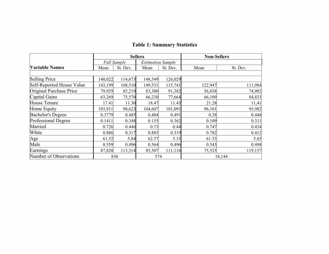
Table 1: Summary Statistics

Sellers Non-SellersFull Sample Estimation Sample

Variable Names Mean St. Dev. Mean St. Dev. Mean St. Dev.

Selling Price 140,022 114,673 148,549 126,029Self-Reported House Value 143,199 108,510 149,531 115,741 122,947 111,984Original Purchase Price 79,929 85,219 83,300 91,382 56,838 74,982Capital Gains 63,269 75,570 66,230 77,664 66,109 84,833House Tenure 17.41 11.30 18.47 11.45 21.28 11,41Home Equity 103,911 98,623 104,607 101,091 96,101 95,982Bachelor's Degree 0.3779 0.485 0.404 0.491 0.28 0.448Professional Degree 0.1411 0.348 0.155 0.362 0.109 0.311Married 0.726 0.446 0.73 0.44 0.747 0.434White 0.886 0.317 0.885 0.319 0.782 0.412Age 61.52 5.84 62.57 5.33 61.53 5.65Male 0.559 0.496 0.564 0.496 0.543 0.498Earnings 87,820 113,314 85,507 111,116 75,525 119,157Number of Observations 836 574 18,144

29

Table 2: The Accuracy of Self-Reported House Values

Dependent Variable: Sale Prices OLS OLS, no constant IV-GMM Corrected IV-GMM Coeff. St. Err. Coeff. St. Err. Coeff. St. Error Coeff. St. Error Self-Reported House Value 0.9066 0.109 0.9129 0.0783 0.9382 0.0519 0.9603 0.0919Months between the report and the sale 795.46 481.22 915.04 564.93 655.9 419.93 711.624 453.099 Constant 3,029 17,090 - - - Inverse Mills ratio - - - -1,767.3 6,685.68 Adj. R-squared 0.6998 0.8744 - - Test of over-identifying restrictions - - Cannot Reject, P-val.=0.78 Cannot Reject, P-val.=0.92 Test of weak instruments - - Reject, F(2,571)=288.54 Reject, F(2,570)=56.26 Number of Observations 574 574 574 574

Table 3: The Role of Capital Gains and Original Purchase Price

Dependent Variable: Sale Prices OLS OLS, no constant IV-GMM Corrected IV-GMM Coeff. St. Err. Coeff. St. Err. Coeff. St. Error Coeff. St. Error Expected Capital Gains 0.8051 0.121 0.8122 0.096 0.91801 0.0576 0.876 0.0918 Original Purchase Price 0.978 0.117 0.9848 0.089 0.999 0.0878 0.9051 0.0754Months between the report and the sale 833.85 485.59 965.23 562.74 550.74 443.10 608.90 440.39 Constant 3,330.68 16,742 - - - Inverse Mills ratio - - - 3,198.78 5,384.6 Adj. R-squared 0.7068 0.8774 - - Test of over-identifying restrictions - - Cannot Reject, P-val.=0.42 Cannot Reject, P-val.=0.32 Test of weak instruments - - Reject, F(2,570)=289.17 Reject, F(2,569)=96.57 Number of Observations 574 574 574 574

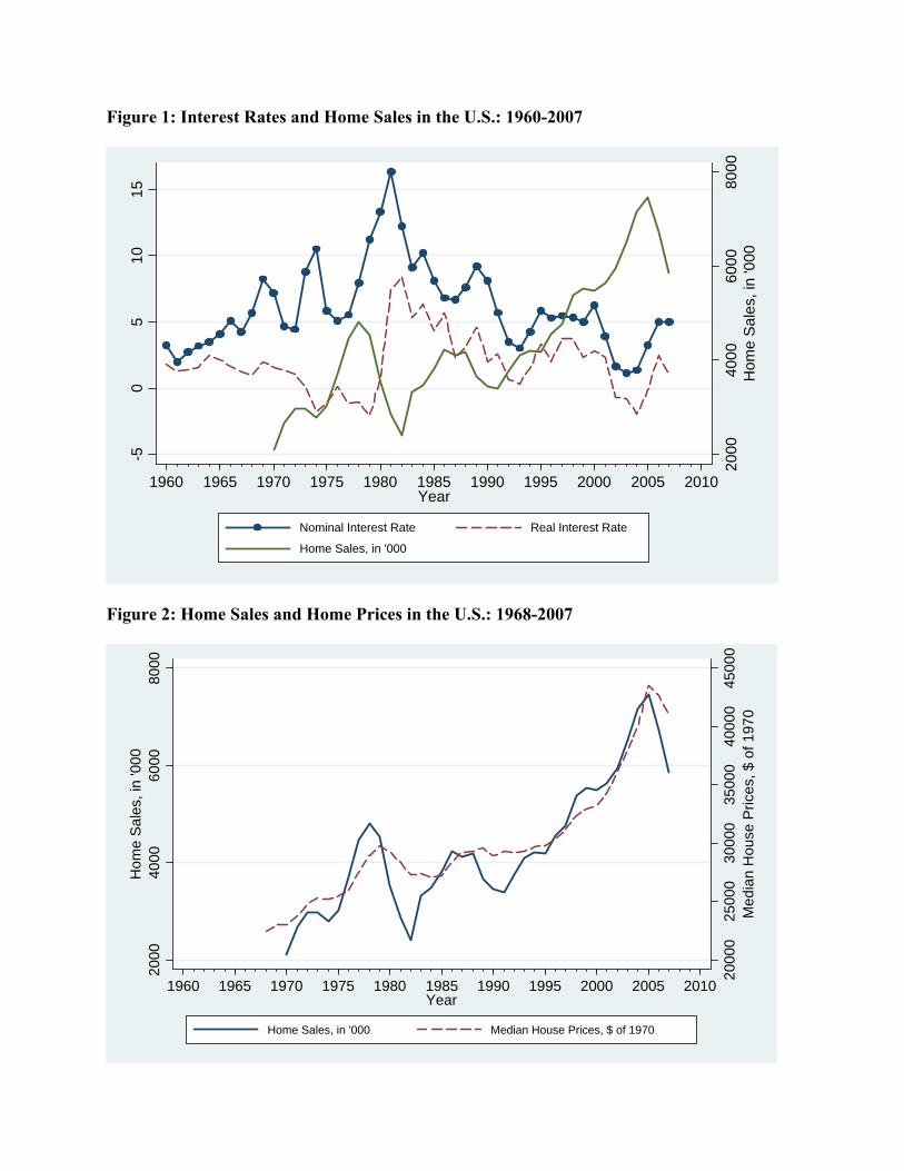
Figure 1: Interest Rates and Home Sales in the U.S.: 1960-2007

2000

4000

6000

8000

Hom

e S

ales

, in

'000

-50

510

15

1960 1965 1970 1975 1980 1985 1990 1995 2000 2005 2010Year

Nominal Interest Rate Real Interest Rate

Home Sales, in '000

Figure 2: Home Sales and Home Prices in the U.S.: 1968-2007

2000

025

000

3000

035

000

4000

045

000

Med

ian

Hou

se P

rices

, $ o

f 197

0

2000

4000

6000

8000

Hom

e S

ales

, in

'000

1960 1965 1970 1975 1980 1985 1990 1995 2000 2005 2010Year

Home Sales, in '000 Median House Prices, $ of 1970

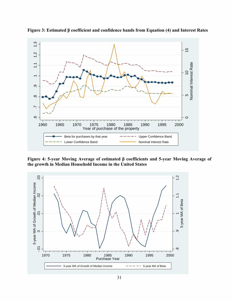
Figure 3: Estimated β coefficient and confidence bands from Equation (4) and Interest Rates

05

1015

Nom

inal

Inte

rest

Rat

e

.6.7

.8.9

11.

11.

21.

3

1960 1965 1970 1975 1980 1985 1990 1995 2000Year of purchase of the property

Beta for purchases by that year Upper Confidence Band

Lower Confidence Band Nominal Interest Rate

Figure 4: 5-year Moving Average of estimated β coefficients and 5-year Moving Average of the growth in Median Household Income in the United States

31

.8.9

11.

11.

25-

year

MA

of B

eta

-.01

0.0

1.0

2.0

35-

year

MA

of G

row

th o

f Med

ian

Inco

me

1970 1975 1980 1985 1990 1995 2000Purchase Year

5-year MA of Growth of Median Income 5-year MA of Beta

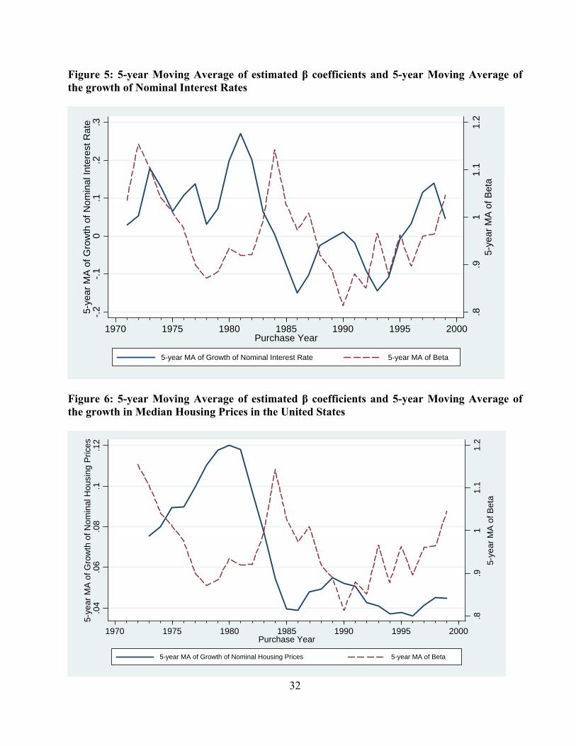
Figure 5: 5-year Moving Average of estimated β coefficients and 5-year Moving Average of the growth of Nominal Interest Rates

.8.9

11.

11.

25-

year

MA

of B

eta

-.2-.1

0.1

.2.3

5-ye

ar M

A o

f Gro

wth

of N

omin

al In

tere

st R

ate

1970 1975 1980 1985 1990 1995 2000Purchase Year

5-year MA of Growth of Nominal Interest Rate 5-year MA of Beta

Figure 6: 5-year Moving Average of estimated β coefficients and 5-year Moving Average of the growth in Median Housing Prices in the United States

32

.8.9

11.

11.

25-

year

MA

of B

eta

.04

.06

.08

.1.1

25-

year

MA

of G

row

th o

f Nom

inal

Hou

sing

Pric

es

1970 1975 1980 1985 1990 1995 2000Purchase Year

5-year MA of Growth of Nominal Housing Prices 5-year MA of Beta