DRAFT PLEASE DO NOT CITE WITHOUT PERMISSION OF THE AUTHORS.

Risk-Benefit Preferences Versus Measured Utility: A Comparison of Methods

F. Reed Johnson George Van Houtven

Research Triangle Institute

10/14/06

Risk-Benefit Preferences Versus Measured Utility: A Comparison of Methods

Health-related decisions often require patients to trade off the health benefits of an

intervention, such as a medical treatment or procedure, against the countervailing risk of a

serious adverse health outcome. Fundamental to these decisions are whether and at what

point the risks outweigh the benefits. In other words, what are the maximum risks patients are

willing to tolerate in exchange for the benefits of the intervention?

Health economists and cognitive psychologists have long studied individuals’

preferences regarding these types of benefit-risk tradeoffs. In particular, standard gamble (SG)

methods are now widely applied to measure health-related utilities for specific conditions.

These utility measures, which primarily are used to support cost-effectiveness analyses, are

derived from surveys where respondents are asked to choose between (1) the certainty of a

specific state of ill health for the remainder of life and (2) a probabilistic lottery involving two

potential outcomes: perfect health for the same period or immediate painless death. Although

other methods also are commonly used, many argue that the SG method is the gold standard

for measuring health utilities (Gold et al., 1996). It offers the advantage of representing

decisions under conditions of uncertainty, which is typical of health related decisions, and it is

based on an established theoretical framework for decision making under uncertainty (Von

Neuman and Morgenstern, 1944).

A number of recent and well-publicized events involving withdrawals of drugs from the

U.S. market (Wysowski and Swartz, 2005) has underscored the importance of understanding

and measuring individuals’ preferences regarding risk-benefit trade-offs. In all of these cases,

interventions offering potentially significant therapeutic benefits were found to carry increased

risks of serious and often life-threatening adverse events. Decisions to halt the development or

sale of these therapies clearly require balancing of benefits and risks; however, establishing

criteria for when the risks outweigh the benefits presents important challenges to decision

makers.

Discrete-choice experiments or conjoint analysis (CA) recently has been proposed and

demonstrated as a multiattribute method for systematically measuring patients’ preferences for

these types of risk-benefit tradeoffs (Johnson et al., 2006). Like the SG method, these

applications of CA use surveys to present individuals with therapeutic choices involving defined

health outcomes and risks. The experimental design of these questions provides a framework,

1

not only for measuring the relative utility individuals associate with different outcomes, but also

for measuring individuals’ maximum acceptable risk (MAR) – i.e., the maximum probability of an

adverse outcome they are willing to tolerate in exchange for a defined therapeutic benefit.

These MAR estimates provide valuable insights into patient preferences, and they should

therefore help to inform risk management decisions that require balancing the risks and benefits

of specific therapies. For example, if average MAR in a patient population is significantly higher

than the actual risks of an adverse outcome, this suggests that the benefits of the treatment

outweigh its risks..

The purpose of this paper is to compare and contrast SG and CA methods for

measuring individuals’ preferences regarding risk-benefit tradeoffs. We compare the empirical

methods used, conceptual frameworks and assumptions used, and types of health preference

measures produced. Using a recent study of patient preferences for Crohn's disease

treatments, we compare empirical preference measures to commonly assumed theoretical

restrictions on admissible functional forms, identify likely biases in conventional SG utility

measures, and suggest an approach for incorporating risk preferences in a recently proposed

extension of cost-effectiveness methods to risk-benefit analysis [Lynd and O’Brien, 2004].

SG and CA methods share a number of similarities when applied to health-related

decision making. First, both are applications of stated-preference methods. That is, they use

surveys to elicit respondent preferences using stated choices for hypothetical health-outcomes

or treatments. Second, the two methods can be used to elicit preferences among hypothetical

choices involving both certain and uncertain health outcomes. Third, both methods can be used

to estimate measures of health utility. Finally, in principle, both CA and SG methods can be

used to measure the maximum acceptable risk (MAR) of a serious adverse health outcome

individuals are willing to tolerate in exchange for a specific health improvement. (Thompson,

1986)

Standard Gamble under Expected and Non-Expected Utility

SG methods are most commonly used to support cost-effectiveness or cost-utility

analyses, where changes in health-related utility are measured in terms of quality adjusted life

years (QALYs). They specifically are used to estimate health-state utility index values for

particular health conditions. These utility indexes typically are expressed on a 0 to 1 scale,

where 0 represents the worst possible outcome, usually death, and 1 represents the best

2

possible outcome, usually perfect health, and thus lower values represent more severe health

states (lower utility). QALYs are calculated by multiplying these health-index constants by the

number (or fraction) of years spent in the corresponding health state.

The conceptual foundation for using SG methods to measure health-related utility is

based on the axioms of expected utility theory (EUT), as initially described by Von Neuman and

Morgenstern (1944). These axioms postulate that individuals implicitly assign utilities to

different outcomes and that, when making decisions under uncertainty, they weight the utilities

of different outcomes according to their respective probabilities of occurring. Individuals

maximize utility under uncertainty by selecting prospects that maximize probability-weighted or

expected utility.

In the typical SG elicitation, survey respondents evaluate two prospects. The first

prospect involves the certainty (probability = 1) of living for a defined period in a specific state of

ill health (H0). The second prospect involves uncertainty, with a lottery between two extreme

outcomes:

• immediate painless death (D) with probability p (0<p<1) and

• perfect health (H1) for the same time period with probability 1-p.

Under EUT, the expected utility (EU) of the uncertain prospect is assumed to be:

)H(U)p1()D(Up)H,D,p(EU 11 ⋅−+⋅= (1)

where U(D) and U(H1) are the utilities of death and perfect health respectively.

The objective of the SG question is to identify the value of p that makes individuals

indifferent between the two prospects. We refer to this value as p*. Although a number of

alternative approaches can be used, in most cases SG methods apply an iterative approach

(“ping-pong” or "bidding-game" method) to arrive at p* (Hammerschmidt, 2004). Rather than

asking respondents to directly state a value for p*, these iterative methods use a series of

discrete choice questions. Respondents are presented with specific values of p and asked to

select their preferred prospect. Depending on how they respond, the value of p is adjusted and

the question is repeated until the individual reaches the point of indifference.

According to EUT, individuals should reach indifference at a value of p* where the

expected utility of the two prospects are equal; therefore, when the utility of death is normalized

to zero and the utility of perfect health is normalized to 1, it follows that

3

*p1)H(U 0 −= (2)

Therefore, 1-p* can be interpreted as a utility index value of the ill-health state H0 as a fraction of

perfect health. In addition, p* can be interpreted as

(1) the MAR of immediate painless death in exchange for improving health from H0 to H1,

and

(2) the instantaneous utility gain or benefit of an improvement from ill health to perfect

health.

Although the EUT framework is widely used to characterize decision making under

uncertainty for health and other areas of applied economics, it also has been widely criticized for

both its positive and normative implications. A large number of empirical studies have

demonstrated systematic violations of the types of behaviors predicted by EUT. (See Starmer,

2000, for a review of this literature.) These findings cast doubt on EUT as a reliable framework

for representing individual preferences and for measuring changes in individual welfare.

One of the main explanations for the observed deviations from EUT is that individuals

may not employ linear probability weighting as required by the theory. Rather, individuals may

systematically adjust probabilities such that, in certain ranges, they receive more weight than

their value and in others they receive less. The result is that probability changes have nonlinear

effects on individuals’ preferences. Two of the main alternatives to EUT that directly address

this type of probability weighting, are rank-dependent utility (RDU) (Quiggin 1993, Yaari 1987)

and prospect theory (Kahneman and Tversky, 1979). Both models depart from EUT by

incorporating nonlinear probability weighting functions in the preference specification1.

Applying the RDU model to the uncertain prospect in an SG framework, preferences can

be expressed as:

)H(U)p1(w)D(U)p(w)H,D,p(RDU 11 ⋅−+⋅= (3)

where w(⋅) is the probability weighting function. This function is a strictly increasing function

with respect to p, such that w(0)=0, w(1)=1, and, for values of p between 0 and 1, w(p) may be

greater than, less than, or equal to p. Importantly, if w(p) = p for all p, then the RDU model is

identical to the EUT model. 1 Prospect theory also includes features that account for the role of reference points in evaluating gains and losses and other commonly observed cognitive anomalies.

4

Empirical evidence on the shape of the probability weighting function comes primarily

from studies examining monetary choices and tradeoffs (Tversky and Kahneman 1992; Wu and

Gonzalez, 1996, Abdellaoui et al.,2006) and only more recently from health-related choices

(Bleichrodt and Pinto 2000). These studies use choice experiments to measure how

respondents’ choices vary with respect to specified changes in probabilities. They typically

assume a functional form for the probability weighting function and use respondent choices to

estimate values for the parameters of these functions. Results from these studies generally

indicate a weighting function with an inverted S-shape, such that w(p)>p for smaller values of p

and w(p)<p for larger values. Examples of weighting functions with this form are shown in

Figure 2.

One of the implications of the probability weighting function under RDU and its observed

S-shape is that the SG method no longer can be interpreted as providing a utility index for a

specific state of ill health (H0). Rather than Eq (2), RDU implies that:

*)*p1(w)H(U 0 −= (4)

where p** is the MAR of immediate painless death (in exchange for an improvement to perfect

health) when preferences are consistent with RDU. Depending on the severity of the health

condition, the SG estimate will either overstate or understate utility. In particular, for relatively

severe conditions, the SG estimate, 1-p**, is likely to understate utility, w(1-p**), while for

relatively mild conditions SG is likely to overstate utility.

Because the conventional SG preference-elicitation format requires that preferences be

linear in probability, it does not yield data to test or estimate properties or parameters of the

probability weighting function. Consequently, it does not allow one to estimate the size of the

potential bias in EUT measures of health utility. The CA method, in contrast, can be used to

explore these properties.

Conjoint Analysis

Rather than imposing a priori restrictions on the functional form preferences may take,

CA methods are based instead on multiattribute, hedonic utility theory. According to hedonic

principles, all “commodities” over which consumers make choices (including therapeutic

treatment options) can be thought of as being composed of a set of attributes. The

attractiveness of a commodity to an individual is a function of these attributes. CA recognizes

5

that individuals place different levels of importance on a commodity’s attributes and, thus, are

willing to accept tradeoffs among them.

When applied to evaluating health preferences, the CA multiattribute choice alternatives

often are framed as “health profiles” associated with possible treatment options. Each

alternative j is described according to a vector of distinct attributes (Xj). This vector might

include several different, but not necessarily mutually exclusive, therapeutic benefits, mild-to-

moderate side effects, and serious adverse-event (SAE) risks associated with the treatment

alternative. Xj may include both continuous and categorical attributes, and the categorical

attributes may or may not be naturally ordered.

In a CA survey, respondents are presented with a series of evaluation tasks involving

choices between two or more treatment options. Each treatment option is described according

to the same attribute categories but the levels of these attributes are varied across options and

across choice tasks according to an experimental design with known statistical properties.

Applying a random utility modeling (RUM) framework and a discrete-choice estimator such as

conditional logit, the observed pattern of respondent choices allows the estimation of preference

parameters (McFadden, 1981) for all attribute levels.

The random utility associated with each alternative is assumed to be a function of these attributes plus a random error term:

β=

ε+=

jj

jjj

XV

VU (5)

where

Vj is the determinate part of the utility function for treatment j;

Xj is a vector of attribute levels for treatment j;

β is a vector of attribute parameters (preference weights); and

εj is a random error.

CA allows for estimation of the relative magnitudes of parameters in the β vector. In addition, by

specifying levels of continuous variables such as SAE risks as categorical, we can directly test

whether preferences are linear in probability or whether they conform to a weighting function

that can be parameterized.

6

CA with linear risk preferences

When the treatment options in a CA survey include attributes that are characterized by

uncertain outcomes – i.e., SAE risks – one option is to assume an EU framework. For example,

assume that treatment options for a specific disease can all be described according to a vector

of attributes Xj . Furthermore, assumed that Xj consists of (1) a vector of efficacy attributes, XBj ,

such as the frequency of disease flare-ups (brief periods of intensified symptoms) and the

severity of day-to-day disease symptoms and (2) a single fatal SAE risk, pj,. In this case the

expected utility of a treatment option j, can be expressed as:

jRBBjjj pX)p1(V β+β−= (6)

where

βB is the vector of attribute parameters in β associated with XB Bj; and

βR is the attribute parameter in β associated with pj

Eq (6) implies that the utility of a treatment option is linear with respect to its SAE risk.

The estimated parameter vector can be used to estimate MAR for selected treatment benefits. If

treatment j provides a higher level of efficacy than treatment i, such that (∆X)βB > 0, the MAR

associated with this higher efficacy benefit is the increased SAE risk from treatment j, ∆p* , that

would make an individual indifferent between treatment i and treatment j. In other words, it is the

increased probability of the SAE with treatment j that would exactly offset its benefits, such that

∆V=0. We thus find MAR as the increase in risk Δp* that equates the difference in expected

utility between two treatments, i and j:

)p()pX(X)p1(VVV RBBjBiij Δβ+Δβ−Δβ−=−=Δ (7)

where ; and BiBj XXX −=Δ ij ppp −=Δ

0*p*pXX)p1(VVV RBBjBiij =Δβ+Δβ−Δβ−=−=Δ (8)

Solving this equation for ∆p* gives us the MAR associated with switching from treatment i to

treatment j.

7

XX)p1(*pMAR

BBjR

Biij Δ

β−ββ−

−=Δ= (9)

Since CA allows us to estimate the relative magnitudes of the parameters in the β vector,

including the βB and βB R parameters, MAR can be directly calculated from the RUM model results

using equation (5).

This derivation of MAR, like an EUT framework, assumes that individuals evaluate

probabilities linearly. That is, as implied by Eq. (6), the marginal effect of adverse side-effect

risks on utility is assumed to be constant so that Rp/V β=∂∂ . Using the CA framework, it is

possible to empirically test this assumption by defining p as a categorical variable and testing

whether there are statistically significant differences in estimated 1kk

1RkRk

pp +

+

−β−β

for all SAE

probability levels k.

This derivation of MAR is also represented in Figure 1. The vertically sloped line

represents the combinations of (1) improvements in efficacy-related benefits, represented by

positive values of (∆X)βB and (2) increases in side-effect risks, represented by positive values of

∆p, that would have exactly offsetting effect on expected utility (i.e., ∆V=0). In this graph, MAR12

is shown as the ∆p that exactly offsets the efficacy-related benefits of switching from treatment 1

to treatment 2 (∆X12 βB). If the benefits of switching from treatment 1 to a third treatment option

(treatment 3) are higher than for treatment 2, then the MAR should also increase. Figure 1

shows this effect, with the benefits of switching to treatment 3 labeled as ∆X

B

13βBB and the higher

corresponding MAR labeled as MAR13.

CA with a probability weighting function

When the treatment options are characterized by uncertain outcomes, CA can also be

adapted to use an RDU framework. To account for potential nonlinearities with respect to risk,

Eq. (10) adapts the preference framework described in Eq (60 by including the probability

weighting function w(p) :

RjBBjjj )p(wX)p1(wV~ β+β−= (10)

8

The change in expected utility between treatment i and j can therefore be rewritten as:

[ ])p(w)p(w)X(X)p1(wV~ ijRBBjBi −β+β−Δβ−=Δ (11)

Setting this equation equal to zero, it is again possible to solve for the MAR that corresponds to

a given increase in efficacy, ∆X. The nonlinearity of this expression with respect to the risk

terms means that MAR will depend on the point of reference for risk. Using the SAE risk from

treatment i as the this point of reference, we assume for simplicity that pi=0, and we solve for

pj** = MAR .

⎥⎥⎦

⎤

⎢⎢⎣

⎡Δ

β−ββ

−== − XX

w**pMARBBjR

B1jij (12)

Existing Empirical Evidence on Probability Weights

Tversky and Kahneman (1992) proposed a single-parameter (γ) probability weighting

function consistent with observations that individuals tend to overweight small probabilities and

underweight large probabilities.

[ ]γγγ

γ

−+= 1

)p1(p

p)p(w 0.27 ≤ γ ≤ 1 (13)

Based on a financial decision making experiment, they estimated the value of γ to be 0.61 for

gains and 0.69 for losses. For health-related decisions, Bleichrodt and Pinto (2000) estimate

values of γ ranging from 0.68 to 0.71. Figure 2 illustrates the effect of various values of γ on the

weighting function.

Other authors have proposed alternative one-parameter and two-parameter weighting

functions with inverse-S shapes similar to Eq (13) (Tversky and Wakker, 1995; Wu and

9

Gonzales, 1996; Prelec, 1998). As previously discussed, the direct implication of inverse-S

weighting functions is that responses to SG questions will yield mortality risk probabilities that,

depending on the severity of the health condition, will either overstate or understate utility as

calculated under expected-utility assumptions. Figure 3 illustrates the difference between SG

responses if utility is linear in probability or nonlinear with γ = 0.6. For relatively severe

conditions and nonlinear probability weighting, the SG estimate, 1-p**, is likely to understate

utility, while for relatively less severe conditions SG is likely to overstate utility.

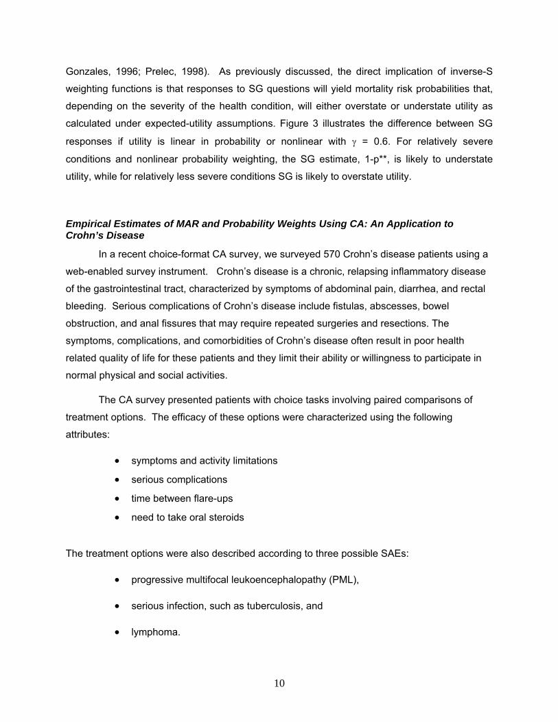
Empirical Estimates of MAR and Probability Weights Using CA: An Application to Crohn’s Disease

In a recent choice-format CA survey, we surveyed 570 Crohn’s disease patients using a

web-enabled survey instrument. Crohn’s disease is a chronic, relapsing inflammatory disease

of the gastrointestinal tract, characterized by symptoms of abdominal pain, diarrhea, and rectal

bleeding. Serious complications of Crohn’s disease include fistulas, abscesses, bowel

obstruction, and anal fissures that may require repeated surgeries and resections. The

symptoms, complications, and comorbidities of Crohn’s disease often result in poor health

related quality of life for these patients and they limit their ability or willingness to participate in

normal physical and social activities.

The CA survey presented patients with choice tasks involving paired comparisons of

treatment options. The efficacy of these options were characterized using the following

attributes:

• symptoms and activity limitations

• serious complications

• time between flare-ups

• need to take oral steroids

The treatment options were also described according to three possible SAEs:

• progressive multifocal leukoencephalopathy (PML),

• serious infection, such as tuberculosis, and

• lymphoma.

10

Each o

this model are shown in Table 1. We then calculated MAR estimates

using th

or

o the

ategorical estimates, while the predicted linear values fit the data very poorly.

SG EstLiterat

timates are difficult to interpret due to a lack of detail

regardi

e CD.

xt,

f these SAE attributes was described in terms of its possible 10 year mortality risks.

Using a random-parameters logit model (Train, 1998) to analyze the respondent choice

data, we first specified the SAE risk levels as categorical variables. This specification imposes

no a priori functional-form requirements regarding the effects of risk on individual utility.

Parameter estimates for

ese estimates.

Table 1 also shows estimates obtained using the standard linear specification and the

weighting function shown in equation (13). Gamma estimates were 0.552, 0.390, and 0.679 f

PML, infection, and lymphoma risks, respectively. All γ estimates were significantly different

from 1 (p<0.01), thus rejecting a linear specification. The lymphoma estimate is similar to those

obtained by Tversky and Kahneman and by Bleichrodt and Pinto. Figures 4a-4c compare plots

of the original categorical estimates with confidence intervals, the probability weighting function,

and the linear estimates. Weighted-probability predicted values correspond closely t

c

imates of MAR and Health Utilities for Crohn’s Disease: Evidence from the ure

Three SG studies have obtained health utility estimates for Crohn’s disease. Kennedy et

al.(2000) surveyed 91 CD patients, 42 percent of whom were in remission. To evaluate the

quality of life changes due to post-operative recurrence of CD symptoms, they estimated SG

scores for a recurrence of CD over 3 years. The resulting average SG utility was 0.91

(SD=0.11); however, the exact timing and severity of the recurrence is not explicit in the study.

Arseneau et al. (2001) also used SG methods with a small sample of both CD patients (N=32)

and healthy individuals (N=20). They estimated utility scores for various symptoms (e.g, fistula,

improved fistula); however, these es

ng their empirical methods.

The study that is the most detailed and comparable to our CA study is Gregor et al.

(1997). The authors surveyed 180 adult CD patients with varying levels of disease severity and

estimated SG utility scores for three hypothetical health states: mild, moderate, and sever

The average scores for these three conditions were 0.81-0.82, 0.72-0.73, and 0.50-0.54

respectively. These utility estimates correspond to MAR values of about 0.20 and 0.10 for

improvements from severe to moderate and from moderate to mild, respectively. In this conte

11

the MAR represents the maximum additional probability of immediate death that patients are

th state.

hat could last weeks or

months t

l.

al

ic γ estimates from the CA study correspond to utility differences ranging from

.017 for γ =0.39 to 0.069 for γ =0.68, much smaller than the 0.10 value obtained under EU

ssumptions.

willing to tolerate to acquire an improvement in their Crohn’s related heal

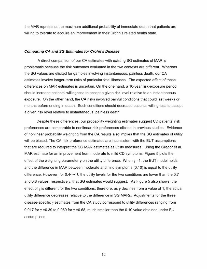
Comparing CA and SG Estimates for Crohn’s Disease

A direct comparison of our CA estimates with existing SG estimates of MAR is

problematic because the risk outcomes evaluated in the two contexts are different. Whereas

the SG values are elicited for gambles involving instantaneous, painless death, our CA

estimates involve longer-term risks of particular fatal illnesses. The expected effect of these

differences on MAR estimates is uncertain. On the one hand, a 10-year risk-exposure period

should increase patients’ willingness to accept a given risk level relative to an instantaneous

exposure. On the other hand, the CA risks involved painful conditions t

before ending in death. Such conditions should decrease patients’ willingness to accep

a given risk level relative to instantaneous, painless death.

Despite these differences, our probability weighting estimates suggest CD patients’ risk

preferences are comparable to nonlinear risk preferences elicited in previous studies. Evidence

of nonlinear probability weighting from the CA results also implies that the SG estimates of utility

will be biased. The CA risk-preference estimates are inconsistent with the EUT assumptions

that are required to interpret the SG MAR estimates as utility measures. Using the Gregor et a

MAR estimate for an improvement from moderate to mild CD symptoms, Figure 5 plots the

effect of the weighting parameter γ on the utility difference. When γ =1, the EUT model holds

and the difference in MAR between moderate and mild symptoms (0.10) is equal to the utility

difference. However, for 0.4<γ<1, the utility levels for the two conditions are lower than the 0.7

and 0.8 values, respectively, that SG estimates would suggest. As Figure 5 also shows, the

effect of γ is different for the two conditions; therefore, as γ declines from a value of 1, the actu

utility difference decreases relative to the difference in SG MARs. Adjustments for the three

disease-specif

0

a

12

Discussion

Systematic deviations from EU assumptions have been extensively observed. It might be

argued that such deviations simply are cognitive errors—people wrongly perceive small risks to

be larger than they actually are and wrongly perceive large risks to be smaller than they actually

are. However, probability weighting appears to be quite pervasive and non-expected utility

models generally explain behavior better than expected utility models. If such behavior were a

cognitive artifact, people would constantly make erroneous decisions without ever learning that

they could improve their welfare by maximizing unweighted expected utility. Rejecting such

revealed preferences requires rejecting the individualistic ethic that is the basis of modern

,” as well as

s.

e implicit

ted incidence of a rare even may be

ignificantly larger than the measured incidence.

economic theory, i.e. that individuals are the best judge of their own utility.

While our interest in this study primarily is in how to elicit valid measures of therapeutic risk

tolerance, our ability to estimate nonlinear risk preferences with CA data offers a direct test of

the expected utility hypothesis for hypothetical, but realistic therapeutic tradeoffs. The SG

method requires analysts to assume the expected utility hypothesis is valid and produces no

empirical test of this essential assumption. Hence our rejection of linear risk preferences has

implications for deriving conventional health utility weights via the SG “gold standard

for interpretation of the reciprocal of utility weights as a measure of risk tolerance.

Although our MAR estimates for CD treatments are smaller than those implied by SG methods,

CD patients appear to be willing to accept significant SAE risks in return for therapeutic benefit

This risk tolerance is greater than observed clinical risks. However, our analysis raises

questions about how to define risk exposures. If patients weight risks subjectively in

determining MAR, then their subjective perception of actual risk exposure should also be

weighted accordingly to compare the implicit utility of the maximum tolerance versus th

utility of the actual risk exposure. Thus the weigh

s

13

REFERENCES

Abdellaoui, M, Barrios C, Wakker P. Reconciling Introspective Utility with Revealed Preferences: Experimental Arguments based on Prospect Theory. Journal of Econometrics 2006; (forthcoming)

Arseneau K, Cohn S, Cominelli F, Connors A. Cost-Utility of Initial Medical Management for Crohn's disease Perianal Fistulae. Gastroenterology 2001; 120:1640-1656.

Bleichrodt H. and Pinto J. The Validity of QALYs Under Non-Expected Utility. The Economic Journal 2005; 115 (April): 533–550.

Gold MR, Siegel JE, Russell LB, Weinstein MC. Cost-Effectiveness in Health and Medicine. Oxford University Press, NY, 1996.

Gregor J, McDonald J, Klar N, Wall R, Atkinson K, Lamba B, Feagan B. An Evaluation of Utility Measurement in Crohn's Disease. Inflammatory Bowel Disease 1997; 3(4):265-276.

Hammerschmidt T, Zeitler H-P, Gulich M, Leidl R. A Comparison of Different Strategies to Collect Standard Gamble Utilities. Med Decis Making 2004; 24: 493-503.

Johnson FR, Özdemir S, Hauber AB, Kauf T. Women’s Willingness to Accept Perceived Risks for Vasomotor Symptom Relief 2006; Working Paper, Research Triangle Institute.

Johnson FR, Mansfield C, Özdemir S, Hass S, White J. Crohn's Disease Patients' Risk-Benefit Preferences: Serious Adverse Event Risks versus Treatment Efficacy 2006; Working Paper, Research Triangle Institute.

Kahneman D and Tversky. Prospect Theory: An Analysis of Decision under Risk. Econometrica 1979; Vol. 47(2): 263 – 92.

Kennedy E, Detsky A, Llewellyn-Thomas H, O'Connor B, Varkul M, Steinhart H, Cohen Z, McLeod R. Can the Standard Gamble Be Used to Determine Utilities for Uncertain Health States? An Example Using Postoperative Maintenance Therapy in Crohn's Disease. Medical Decision Making 2000; 20(1):72-78.

Lynd LF, and O’Brien BJ. Advances in Risk-benefit Evalaution Using Probabilistic Simulation Methods: An Application to the Prophyulaxis of Deep Vein Thrombosis. Journal of Clinical Epidemiology 2004; 57, 795-803.

McFadden, D. Econometric models of probabilistic choice. In: Manski, CF and McFadden D. (Eds.), Structural Analysis of Discrete Data with Economic Applications. MIT Press, Boston, 422–434. 1981.

Prelec, D. The Probability Weighting Function. Econometrica 1998; 66, 497-527.

Quiggin J. Generalized Expected Utility Theory: The Rank-Dependent Model. Boston: Kluwer. 1993.

Starmer C. Developments in Non-Expected Utility Theory: The Hunt for a Descriptive Theory of Choice Under Risk. Journal of Economic Literature 2000; XXXVIII: 332-82.

Thompson M. Willingness to Pay and Accept Risks to Cure Chronic Disease American Journal of Public Health 1986; 76(4):392-396

Train K. Recreation Demand Models with Taste Differences Over People. Land Economics 1998, 74 (2), 230-239

14

Tversky A and Kahneman D. Advances in Prospect Theory: Cumulative Representation of Uncertainty’, Journal of Risk and Uncertainty 1992; 5: 297–323.

Tversky A and Kahneman D. (1992). Advances in Prospect Theory: Cumulative Representation of Uncertainty. Journal of Risk and Uncertainty. 1992; 5: 297–323.

Tversky A, and Wakker P. Risk Attitudes and Decision Weights. Econometrica 1995; 63:1255-1280.

Von Neumann J and Morgenstern O. Theory of Games and Economic Behavior. Princeton University Press, NJ, 1944.

Wu G. and Gonzalez R. Curvature of the Probability Weighting Function, Management Science 1996; 42:1676-1690.

Wysowski, Diane K. and Lynette Swartz. 2005. “Adverse Drug Event Surveillance and Drug Withdrawals in the United States, 1969-2002.” Archives of InternalMedicine 165:1363-69.

Yaari M. The Dual Theory of Choice Under Risk. Econometrica 1987; 55:95-115.

15

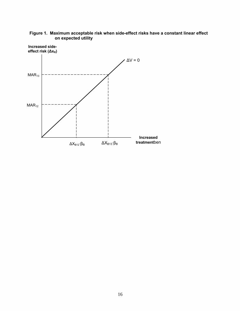
Figure 1. Maximum acceptable risk when side-effect risks have a constant linear effect on expected utility

ΔV = 0

Increased treatmentbenΔXB12·βB ΔXB13·βB

MAR12

MAR13

Increased side-effect risk (ΔxR)

16

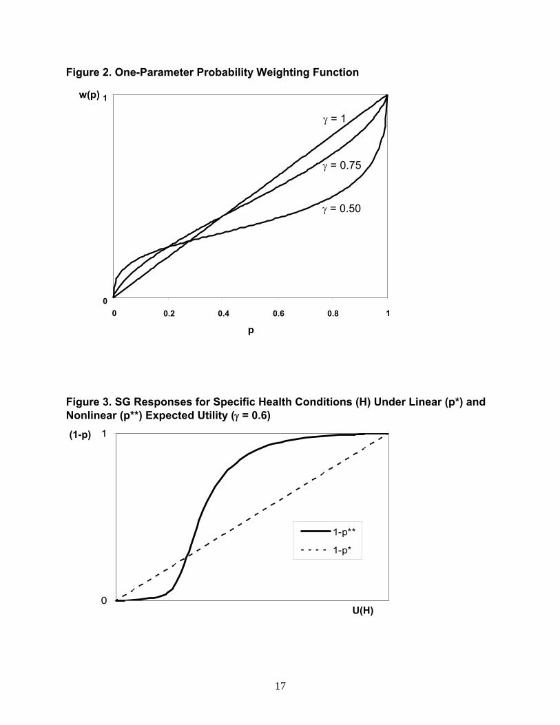
Figure 2. One-Parameter Probability Weighting Function

0

1

0 0.2 0.4 0.6 0.8 1

p

w(p)

γ = 1

γ = 0.75

γ = 0.50

Figure 3. SG Responses for Specific Health Conditions (H) Under Linear (p*) and Nonlinear (p**) Expected Utility (γ = 0.6)

(1-p)

0

1

1-p**

1-p*

U(H)

17

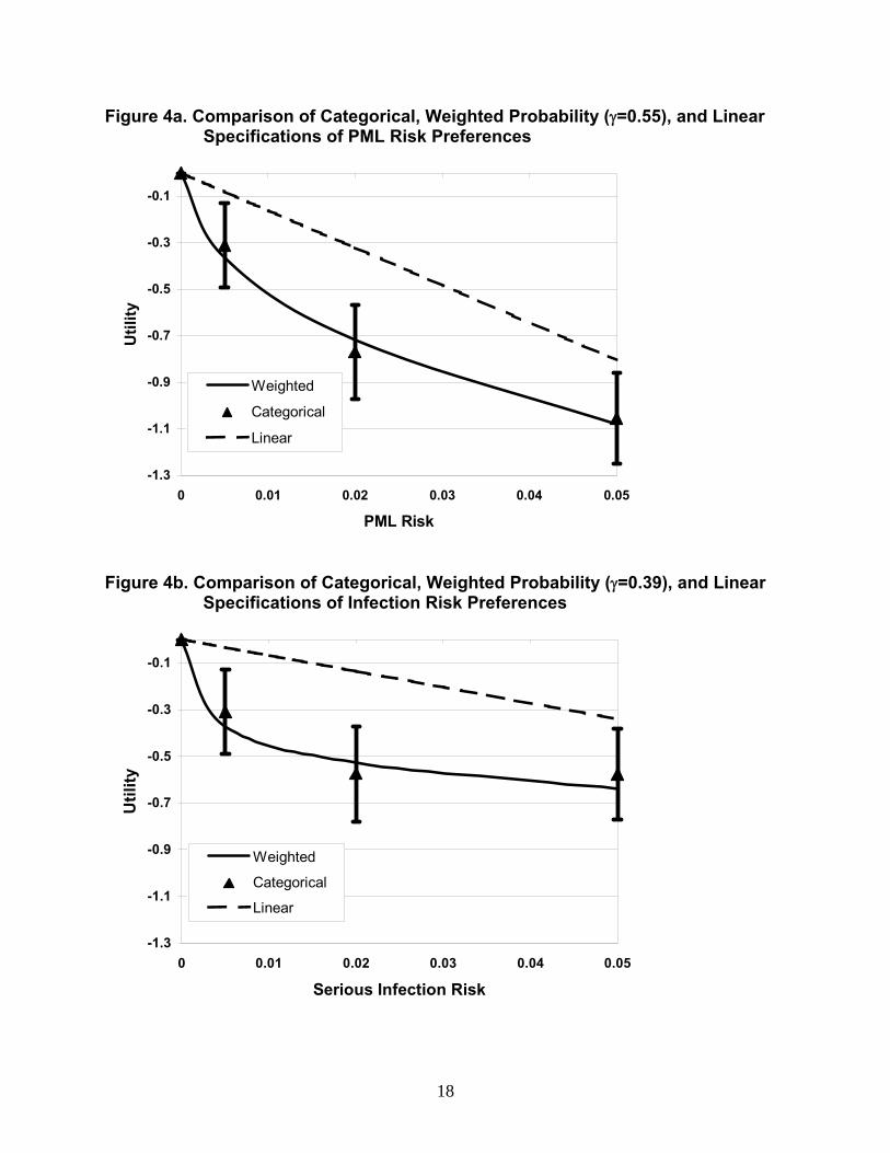
Figure 4a. Comparison of Categorical, Weighted Probability (γ=0.55), and Linear Specifications of PML Risk Preferences

-1.3

-1.1

-0.9

-0.7

-0.5

-0.3

-0.1

0 0.01 0.02 0.03 0.04 0.05

PML Risk

Util

ity

Weighted

Categorical

Linear

Figure 4b. Comparison of Categorical, Weighted Probability (γ=0.39), and Linear Specifications of Infection Risk Preferences

-1.3

-1.1

-0.9

-0.7

-0.5

-0.3

-0.1

0 0.01 0.02 0.03 0.04 0.05

Serious Infection Risk

Util

ity

Weighted

Categorical

Linear

18

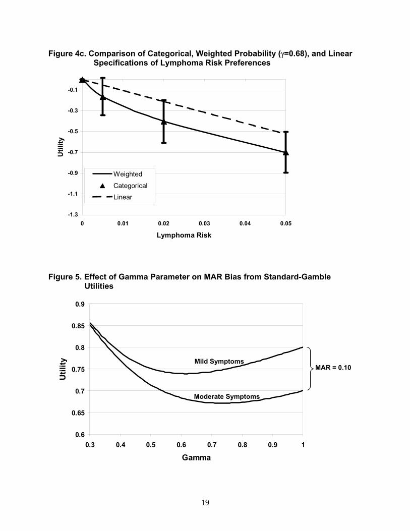
Figure 4c. Comparison of Categorical, Weighted Probability (γ=0.68), and Linear Specifications of Lymphoma Risk Preferences

-1.3

-1.1

-0.9

-0.7

-0.5

-0.3

-0.1

0 0.01 0.02 0.03 0.04 0.05

Lymphoma Risk

Util

ity

Weighted

Categorical

Linear

Figure 5. Effect of Gamma Parameter on MAR Bias from Standard-Gamble Utilities

0.6

0.65

0.7

0.75

0.8

0.85

0.9

0.3 0.4 0.5 0.6 0.7 0.8 0.9 1

Gamma

Util

ity

Mild Symptoms MAR = 0.10

Moderate Symptoms

19

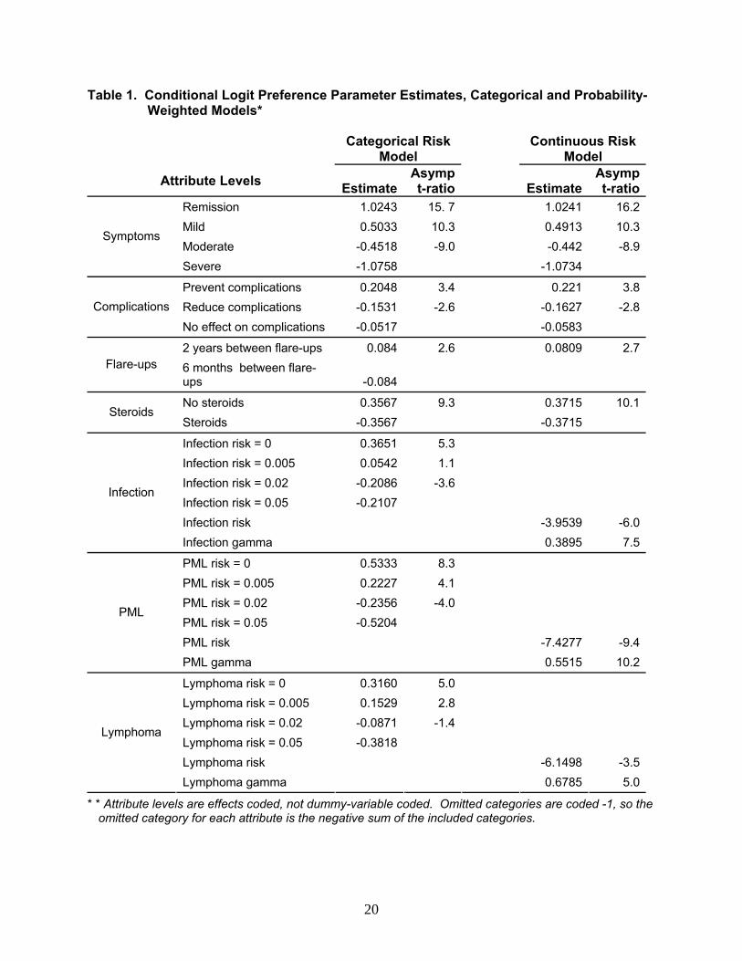
Table 1. Conditional Logit Preference Parameter Estimates, Categorical and Probability-Weighted Models*

Categorical Risk

Model Continuous Risk

Model

Attribute Levels EstimateAsymp t-ratio Estimate

Asymp t-ratio

Remission 1.0243 15. 7 1.0241 16.2Mild 0.5033 10.3 0.4913 10.3Moderate -0.4518 -9.0 -0.442 -8.9

Symptoms

Severe -1.0758 -1.0734

Prevent complications 0.2048 3.4 0.221 3.8Reduce complications -0.1531 -2.6 -0.1627 -2.8Complications

No effect on complications -0.0517 -0.0583

2 years between flare-ups 0.084 2.6 0.0809 2.7Flare-ups 6 months between flare-

ups -0.084

No steroids 0.3567 9.3 0.3715 10.1Steroids

Steroids -0.3567 -0.3715

Infection risk = 0 0.3651 5.3 Infection risk = 0.005 0.0542 1.1 Infection risk = 0.02 -0.2086 -3.6 Infection risk = 0.05 -0.2107 Infection risk -3.9539 -6.0

Infection

Infection gamma 0.3895 7.5

PML risk = 0 0.5333 8.3 PML risk = 0.005 0.2227 4.1 PML risk = 0.02 -0.2356 -4.0 PML risk = 0.05 -0.5204 PML risk -7.4277 -9.4

PML

PML gamma 0.5515 10.2

Lymphoma risk = 0 0.3160 5.0 Lymphoma risk = 0.005 0.1529 2.8 Lymphoma risk = 0.02 -0.0871 -1.4 Lymphoma risk = 0.05 -0.3818 Lymphoma risk -6.1498 -3.5

Lymphoma

Lymphoma gamma 0.6785 5.0

* * Attribute levels are effects coded, not dummy-variable coded. Omitted categories are coded -1, so the omitted category for each attribute is the negative sum of the included categories.

20