Embed Size (px)
Citation preview
Evaluating Ecosystem Effects of Oyster Restoration in Chesapeake Bay
A Report to the Maryland Department of Natural Resources
September 2005
Carl F. Cerco and Mark R. Noel
US Army Engineer Research and Development Center, Vicksburg MS
Abstract
The Chesapeake Bay Environmental Model Package (CBEMP) was used to assess the environmental benefits of oyster restoration in Chesapeake Bay. The CBEMP consists of a coupled system of models including a three-dimensional hydrodynamic model, a three-dimensional eutrophication model, and a sediment diagenesis model. Restoration levels up to fifty times the 1994 base biomass were examined. Examination of results emphasized dissolved oxygen, chlorophyll concentration, and water clarity. Within Virginia , the improvement in summer, bottom-water dissolved oxygen at the maximum biomass investigated was 0.2 mg/L. Within Maryland, the improvement was doubled, more than 0.4 mg/L. Within Virginia, the range of oyster densities investigated reduced summer-average surface chlorophyll by up to ˜ 0.7 µg/L, roughly 10% of the 1994 base concentration. Corresponding reductions in Maryland were up to ˜ 2.3 µg/L, more than 25% of the 1994 base. Within Virginia, the range of oyster densities investigated reduced summer-average light attenuation by up to 8%, from 1.05 m-1 at base levels to 0.97 m-1 for a fifty-fold increase in oyster biomass. Following a pattern established for other benefits, improvements in Maryland exceeded Virginia. Summer-average light attenuation diminished by up to 13%, from 1.39 m-1 under base conditions to 1.21 m-1 for a fifty-fold increase in oyster biomass.
Ecosystem services performed by oysters include nitrogen removal and
SAV restoration. The range of oyster densities investigated removed up to 24,600 kg d-1 nitrogen in Maryland and up to 5,100 kg d-1 in Virginia. Relative improvements in SAV biomass were greater than corresponding reductions in light attenuation. Percentage increases in summer SAV biomass in Virginia were up to 21%. Computed SAV biomass increased from 5,627 tonnes C under base conditions to 6,830 tonnes for a fifty-fold oyster restoration. In Maryland, improvements in SAV biomass were up to 43%. Computed summer SAV biomass increased from 5,227 tonnes C under base conditions to 7,486 tonnes C under maximum restoration. Point of Contact Carl F. Cerco, PhD, PE Research Hydrologist Mail Stop EP-W US Army ERDC 3909 Halls Ferry Road Vicksburg MS 39180 USA 601-634-4207 (voice) 601-634-3129 (fax) [email protected]
Chapter 1 Introduction 1
1 Introduction
Oyster biomass and harvest in the Chesapeake Bay system have been declining exponentially since the nineteenth century (Rothschild et al. 1994, Kirby and Miller 2005). A link between decimation of the oyster population and deteriorating water quality in Chesapeake Bay was proposed by Newell (1988). Newell calculated the nineteenth-century oyster population could filter the entire volume of the bay in less than a week and suggested an increase in the oyster population could significantly improve water quality by removing large quantities of particulate carbon. While Newell’s proposition was not universally accepted (e.g. Gerritsen et al. 1994), the idea that managing the natural resource can improve water quality has fascinated scientists and managers since the proposition was advanced.
The potential links between living resources and water quality are central
to the “Chesapeake 2000” agreement, signed by the executives of the Commonwealth of Pennsylvania, the State of Maryland, the Commonwealth of Virginia, the District of Columbia, the US Environmental Protection Agency, and the Chesapeake Bay Commission. The agreement sets specific goals including:
Restore, enhance and protect the finfish, shellfish and other living resources, their habitats and ecological relationships to sustain all fisheries and provide for a balanced ecosystem.
The agreement lists methods to achieve this goal including:
By 2010, achieve, at a minimum, a tenfold increase in native oysters in the Chesapeake Bay, based on a 1994 baseline.
and
By 2004, assess the effects of different population levels of filter feeders such as menhaden, oysters and clams on Bay water quality and habitat.
The environmental effects of a ten-fold increase in population of native oysters were assessed by incorporating oysters into the Chesapeake Bay Environmental Model Package (CBEMP), a comprehensive mathematical model of physical and eutrophication processes in the bay and its tidal tributaries (Cerco and Noel 2005).
Chapter 1 Introduction 2
The decline of the native oyster, Crassostrea virginica, has been attributed to overfishing (Jordan and Coakley 2004), disease (Andrews 1965, Andrews 1988), and habitat destruction (Rothschild et al. 1994, Kirby and Miller 2005). The intractable problem of disease has led to the proposal to introduce a disease-resistant exotic oyster, Crassostrea ariakensis, to the Chesapeake Bay system. The Maryland Department of Natural Resources (DNR) and other organizations have initiated a wide range of studies to evaluate the environmental impact of oyster restoration and of C. ariakensis introduction. These studies fall under the heading of Ecological Risk Assessment (ERA) and will be summarized in a Programmatic Environmental Impact Statement (EIS). This report provides information for the ERA and EIS by evaluating several endpoints related to ecosystem impacts of the oyster restoration effort. This work addresses, among other factors, oyster impact on dissolved oxygen, algal biomass, light penetration, and submerged aquatic vegetation (SAV) abundance. The Chesapeake Bay Environmental Model Package
Three models are at the heart of the CBEMP. Distributed flows and loads from the watershed are computed with a highly-modified version of the HSPF model (Bicknell et al. 1996). These flows are input to the CH3D-WES hydrodynamic model (Johnson et al. 1993) that computes three-dimensional intra-tidal transport. Computed loads and transport are input to the CE-QUAL-ICM eutrophication model (Cerco and Cole 1993) which computes algal biomass, nutrient cycling, and dissolved oxygen, as well as numerous additional constituents and processes. The eutrophication model incorporates a predictive sediment diagenesis component (DiToro and Fitzpatrick 1993) as well as living resources including benthos (Meyers et al. 2000), zooplankton (Cerco and Meyers 2000), and submerged aquatic vegetation (Cerco and Moore 2001).
A revision of the CBEMP was delivered in 2002 (Cerco and Noel 2004) and used in development of the most recent nutrient and solids load allocations in the bay. This version of the model was used to examine the impact of the tenfold increase in native oysters (Cerco and Noel 2005). The same version is used here to examine ecological effects of a wider range of restored oyster biomass. The 2002 CBEMP employs nutrient and solids loads from Phase 4.3 of the watershed model (Linker et al. 2000). (Documentation may be found on the Chesapeake Bay Program web site http://www.chesapeakebay.net/modsc.htm.) Nutrient and solids loads are computed on a daily basis for 94 sub-watersheds of the 166,000 km2 Chesapeake Bay watershed and are routed to individual model cells based on local watershed characteristics and on drainage area contributing to the cell. The hydrodynamic and eutrophication models operate on a grid of 13,000 cells. The grid contains 2,900 surface cells (.4 km2) and employs non-orthogonal curvilinear coordinates in the horizontal plane. Z coordinates are used in the vertical direction, which is up to 19 layers deep. Depth of the surface cells is 2.1 m at mean tide and varies as a function of tide, wind, and other forcing functions. Depth of sub-surface cells is fixed at 1.5 m. A band of littoral cells, 2.1 m deep at mean tide, adjoins the shoreline throughout most of the system. Ten years, 1985-1994, are simulated continuously using time steps of .5 minutes (hydrodynamic model) and .15 minutes (eutrophication model).
Chapter 1 Introduction 3
Critical Assumptions Baseline rules and critical assumptions were made at the commencement of the study. These were forced by available knowledge (or lack thereof) and by the requirement to produce a valid product within a reasonable time frame. Mass-Balance Based Model
Our approach models oysters from a mass-balance perspective. Oyster biomass is computed as a function of food availability, respiration, and mortality. Environmental effects on life processes are explicitly considered so that filtering capacity is consistent with environmental conditions. Our approach emphasizes the spatial and temporal distributions of filtering capacity and the environmental effects of filtering and deposition. Population processes including recruitment and larval setting are not considered. The demographic modeling conducted as a part of the larger EIS effort includes population effects not considered here. Equivalence of C. virginica and C. ariakensis The oyster model incorporated into the CBEMP considers market-sized native oysters and is parameterized to the greatest extent possible with local observations. Insufficient information exists to distinguish C. ariakensis from C. virginica within the model. Available information suggests model parameters adopted for native oysters apply to the exotic oysters as well. Preliminary laboratory experiments (National Research Council 2004) indicate size-specific filtration rates for C. ariakensis are similar to those of C. virginica. Mann (2005) concluded there is no reason filtration rates should differ significantly between the two species. These findings are consistent with conclusions of Powell et al. (1992) that size-specific filtration rates are similar for most marine bivalve species. Historical Spatial Distribution Our approach restricts oysters to their historical locations. This approach is reasonable in view of oysters’ affinity for specific bottom types. More elaborate restoration schemes including the creation of new habitat or the construction of rafts can be readily modeled but are left for future investigations. Spatially-Uniform Mortality Rates The model combines mortality from harvest, predation, and disease into a single first-order mortality term. In the absence of any information, this term is considered to be spatially uniform throughout the system. Non-uniform mortality rates can be added to the model as a future effort. References Andrews, J. (1965). “Infection experiments in nature with Dermocystidium
marinum in Chesapeake Bay,” Chesapeake Science, 6:60-67.
Chapter 1 Introduction 4
Andrews, J. (1988). “Epizoology of the disease caused by the oyster pathogen Perkinsus marinus and its effect on the oyster industry,” American Fisheries Society Special Publication, 18:47-63.
Bicknell, B., Imhoff, J., Kittle, J., Donigian, A., Johanson, R., and Barnwell, T.
(1996). “Hydrologic simulation program - FORTRAN user’s manual for release 11,” United States Environmental Protection Agency Environmental Research Laboratory, Athens GA.
Cerco, C., and Cole, T. (1993). “Three-dimensional eutrophication model of
Chesapeake Bay,” Journal of Environmental Engineering, 119(6), 1006-10025.
Cerco, C., and Meyers, M. (2000). “Tributary refinements to the Chesapeake Bay
Model,” Journal of Environmental Engineering, 126(2), 164-174. Cerco, C., and Moore, K. (2001). “System-wide submerged aquatic vegetation
model for Chesapeake Bay,” Estuaries, 24(4), 522-534. Cerco, C., and Noel, M. (2004). “The 2002 Chesapeake Bay eutrophication
model,” EPA 903-R-04-004, Chesapeake Bay Program Office, US Environmental Protection Agency, Annapolis, MD. (available at http://www.chesapeakebay.net/modsc.htm)
Cerco, C., and Noel, M. (2005). “Assessing a ten-fold increase in the Chesapeake
Bay native oyster population,” Chesapeake Bay Program Office, US Environmental Protection Agency, Annapolis, MD. (available at http://www.chesapeakebay.net/modsc.htm)
DiToro, D., and Fitzpatrick, J. (1993). “Chesapeake Bay sediment flux model,”
Contract Report EL-93-2, US Army Engineer Waterways Experiment Station, Vicksburg, MS.
Gerritsen, J., Holland, A., and Irvine, D. (1994). “Suspension-feeding bivalves
and the fate of primary production: An estuarine model applied to Chesapeake Bay,” Estuaries, 17(2), 403-416.
Johnson, B., Kim, K., Heath, R., Hsieh, B., and Butler, L. (1993). “Validation of
a three-dimensional hydrodynamic model of Chesapeake Bay,” Journal of Hydraulic Engineering, 199(1), 2-20.
Jordan, S., and Coakley, J. (2004). “Long-term projections of eastern oyster
populations under various management scenarios,” Journal of Shellfish Research, 23(1):63-72.
Kirby, M., and Miller, H. (2005). “Response of a benthic suspension feeder
(Crassostrea virginica Gmelin) to three centuries of anthropogenic eutrophication in Chesapeake Bay,” Estuarine Coastal and Shelf Science, 62:679-689.
Chapter 1 Introduction 5
Linker, L., Shenk, G., Dennis, R., and Sweeney, J. (2000). “Cross-media models of the Chesapeake Bay watershed and airshed,” Water Quality and Ecosystem Modeling, 1(1-4), 91-122.
Mann, R. (2005). Presentation at June 28-29 Independent Oyster EIS Advisory
Panel meeting. Meyers, M., DiToro, D., and Lowe, S. (2000). “Coupling suspension feeders to
the Chesapeake Bay eutrophication model,” Water Quality and Ecosystem Modeling, 1(1-4), 123-140.
National Research Council. (2004). “Oyster biology.” Nonnative oysters in the
Chesapeake Bay. National Academy Press, Washington, DC, 93. Newell, R. (1988). “Ecological changes in Chesapeake Bay: Are they the result
of overharvesting the American oyster (Crassostrea virginica)?,” Understanding the estuary – Advances in Chesapeake Bay Research. Publication 129, Chesapeake Research Consortium, Baltimore, 536-546.
Powell, E., Hofmann, E., Klink, J., and Ray, S. (1992). “Modeling oyster
populations. I. A commentary on filtration rate. Is faster always better?,” Journal of Shellfish Research, 11, 387-398.
Rothschild, B., Ault, J., Goulletquer, P., and Heral, M. (1994). “Decline of the
Chesapeake Bay oyster population: a century of habitat destruction and overfishing,” Marine Ecology Progress Series, 111, 29-39.
Chapter 2 The Oyster Model 1
2 The Oyster Model
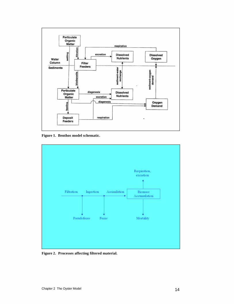
Introduction The ultimate aim of eutrophication modeling is to preserve precious living resources. Usually, the modeling process involves the simulation of living-resource indicators such as dissolved oxygen. For the “Virginia Tributary Refinements” phase of the Chesapeake Bay modeling (Cerco et al. 2002), a decision was made to initiate direct interactive simulation of three living resource groups: zooplankton, benthos, and SAV. Benthos were included in the model because they are an important food source for crabs, finfish, and other economically and ecologically significant biota. In addition, benthos can exert a substantial influence on water quality through their filtering of overlying water. Benthos within the model were divided into two groups: deposit feeders and filter feeders (Figure 1). The deposit-feeding group represents benthos that live within bottom sediments and feed on deposited material. The filter-feeding group represents benthos that live at the sediment surface and feed by filtering overlying water. The primary reference for the benthos model (HydroQual, 2000) is available on-line at http://www.chesapeakebay.net/modsc.htm. Less comprehensive descriptions may be found in Cerco and Meyers (2000) and in Meyers at al. (2000). The benthos model incorporates three filter-feeding groups: 1) Rangea cuneata , which inhabit oligohaline and lower mesohaline portions of the system; 2) Macoma baltica, which inhabit mesohaline portions of the system; and 3) Corbicula fluminea, which are found in the tidal fresh portion of the Potomac. These organisms were selected based on their dominance of total filter-feeding biomass and on their widespread distribution. The distributions of the organisms within the model grid were assigned based on observations from the Chesapeake Bay benthic monitoring program (http://www.chesapeakebay.net/data/index.htm). Oysters were neglected in the initial application of the benthos model. The primary reasoning was that oyster biomass was considered negligible relative to the most abundant organisms.
Oysters The oyster model builds on the concepts established in the benthos model. The existing benthos model was left untouched. The code was duplicated and one portion was modified for specific application to native
Chapter 2 The Oyster Model 2
oysters, Crassostrea virginica. The original model assigned one of the three species exclusively to a model cell. In the revised model, oysters may coexist and compete with the other filter feeders. The fundamental state variable is oyster carbon, quantified as mass per unit area. The minimum area represented is the quadrilateral model cell, which is typically 1 to 2 km on a side. Oyster biomass and processes are averaged over the cell area. Oysters filter particulate matter, including carbon, nitrogen, phosphorus, silica, and inorganic solids from the water column. Particulate matter is deposited in the sediments as feces and pseudofeces. Respiration removes dissolved oxygen from the water column while excretion returns dissolved nitrogen and phosphorus. Particulate carbon is removed from the water column by the filtration process. Filtration rate is affected by temperature, salinity, suspended solids concentration, and dissolved oxygen. The amount of carbon filtered may exceed the oyster’s ingestion capacity. In that case, the excess of filtration over ingestion is deposited in the sediments as pseudofeces (Figure 2). A portion of the carbon ingested is refractory or otherwise unavailable for nutrition. The unassimilated fraction is deposited in the sediments as feces. Biomass accumulation (or diminishment) is determined by the difference between carbon assimilated and lost through respiration and mortality. Respiration losses remove dissolved oxygen from the water column. Mortality losses are deposited to the sediments as particulate carbon. The nutrients nitrogen and phosphorus constitute a constant fraction of oyster biomass. Particulate nitrogen and phosphorus, filtered from the water column, are subject to ingestion and assimilation. Assimilated nutrients that are not accumulated in biomass or lost to the sediments through mortality are excreted to the water column in dissolved inorganic form. All filtered particulate silica is deposited to the sediments or excreted to the water column. A fraction (˜ 10%) of filtered inorganic solids is deposited to the sediments. The fraction is determined by the net settling velocity specified in the suspended solids algorithms. The remainder is considered to be resuspended.
The mass-balance equation for oyster biomass is:
( ) OOBMORFIFPOCFrtd
Od⋅−⋅−⋅−⋅⋅⋅⋅= βα 1 (1)
in which: O = oyster biomass (g C m-2) a = assimilation efficiency (0 < a < 1) Fr = filtration rate (m3 g-1 oyster carbon d-1) POC = particulate organic carbon in overlying water (g m-3) IF = fraction ingested (0 < IF < 1) RF = respiratory fraction (0 < RF < 1) BM = basal metabolic rate (d-1) ß = specific mortality rate (d-1) t = time (d)
Chapter 2 The Oyster Model 3
The assimilation efficiency is specified individually for each form of particulate organic matter in the water column. The respiratory fraction represents active respiratory losses associated with feeding activity. Basal metabolism represents passive respiratory losses. Filtration
Filtration rate is represented in the model as a maximum or optimal rate that is modified by ambient temperature, suspended solids, salinity, and dissolved oxygen:
max)()()()( FrDOfSfTSSfTfFr ⋅⋅⋅⋅= (2)
in which: f(T) = effect of temperature on filtration rate (0 < f(T) < 1) f(TSS) = effect of suspended solids on filtration rate (0 < f(TSS) < 1) f(S) = effect of salinity on filtration rate (0 < f(S) < 1) f(DO) = effect of dissolved oxygen on filtration rate (0 < f(DO) < 1) Frmax = maximum filtration rate (m3 g-1 oyster carbon d-1)
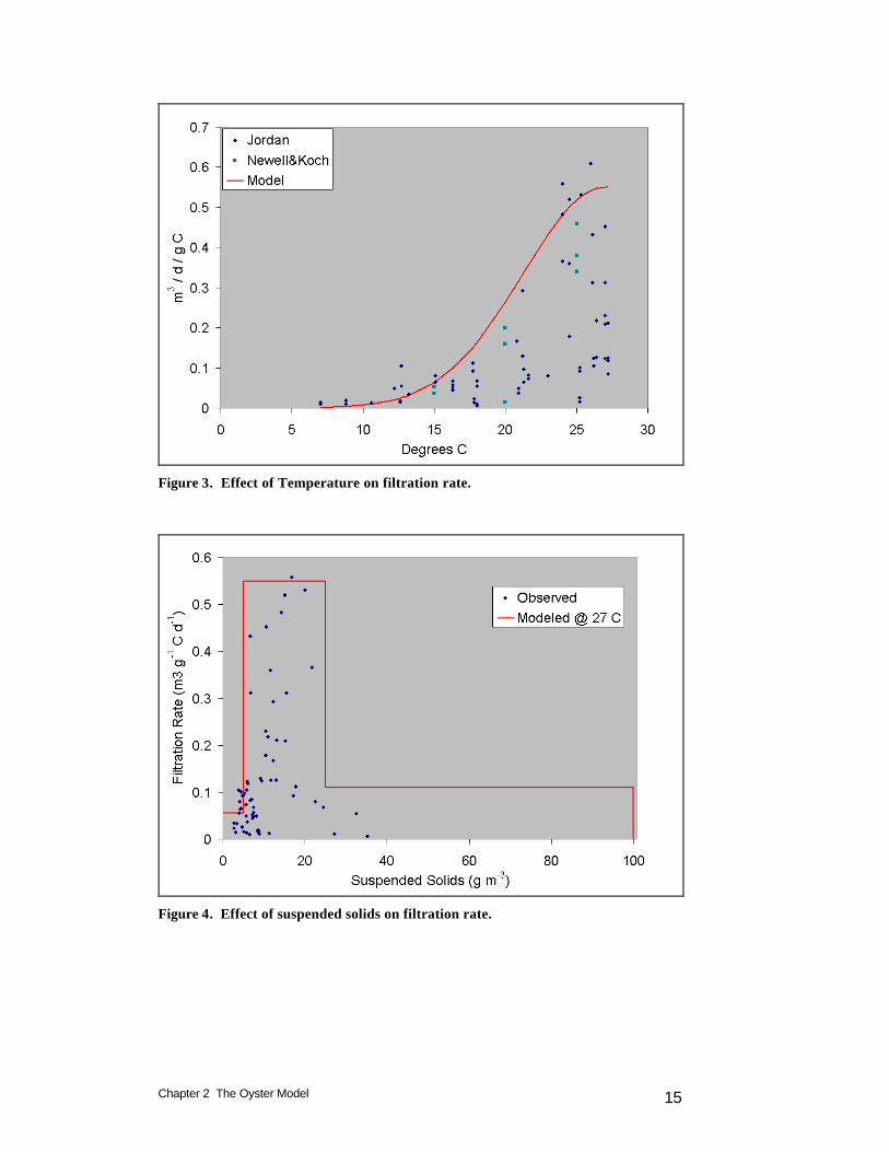
Bivalve filtration rate, quantified as water volume cleared of particles per unit biomass per unit time (Winter 1978), is typically derived from observed rates of particle removal from water overlying a known bivalve biomass (Doering et al. 1986, Doering and Oviatt 1986, Riisgard 1988, Newell and Koch 2004). Since particle retention depends on particle size and composition (Riisgard 1988, Langdon and Newell 1990), correct quantification of filtration requires a particle distribution that represents the natural distribution in the study system (Doering and Oviatt 1986). Filtration rate for our model was based primarily on measures (Jordan 1987) conducted in a laboratory flume maintained at ambient conditions in the adjacent Choptank River, a mesohaline Chesapeake Bay tributary that supports a population of native oysters. These were supplemented with laboratory measures conducted on oysters removed from the same system (Newell and Koch 2004). Jordan reported weight-specific biodeposition rate as a function of temperature, suspended solids concentration and salinity. The biodeposition rate represents a minimum value for filtration since all deposited material is first filtered. Filtration rate was derived:
TSSWBRFr = (3)
in which: WBR = weight-specific biodeposition rate (mg g-1 dry oyster weight hr-1) TSS = total suspended solids concentration (mg L-1) Filtration rate was converted from L g-1 DW h-1 to model units based on a carbon-to-dry-weight ratio of 0.5. The observed rates indicate a strong dependence of filtration on temperature (Figure 3) although the range of filtration rates observed at any
Chapter 2 The Oyster Model 4
temperature indicate the influence of other factors as well. The maximum filtration rate and the temperature dependence for use in the model are indicated by a curve drawn across the highest filtration rates at any temperature:
( )2
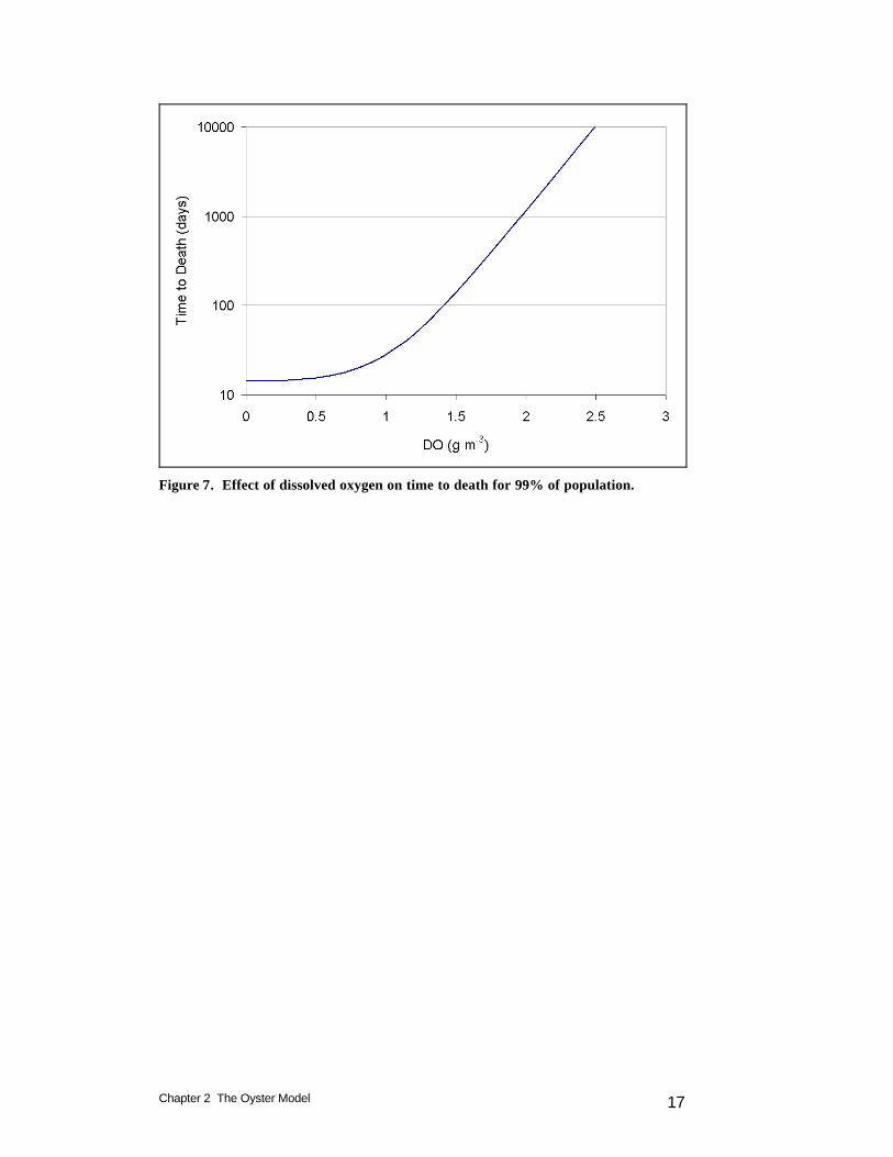
max ToptTKtgeFrFr −⋅−⋅= (4) in which: Frmax = maximum filtration rate (0.55 m3 g-1 oyster carbon d-1) Ktg = effect of temperature on filtration (0.015 oC-2) T = temperature for optimal filtration (27 oC) Suspended Solids Effects. The deleterious effect of high suspended solids concentrations on oyster filtration rate has been long recognized although the solids concentrations induced in classic experiments, 102 to 103 g m-3 (Loosanoff and Tommers 1948), are extreme relative to concentrations commonly observed in Chesapeake Bay. We formed our solids function by recasting Jordan’s data to show filtration rate as a function of suspended solids concentration (Figure 4). The experiments indicate three regions. Filtration rate was depressed when solids were below ˜ 5 gm m-3 and above ˜ 25 gm m-3, relative to filtration rate when solids were between these two levels. The observations suggest oysters reduce their filtration rate when food is unavailable or when filtration at the maximum rate removes vastly more particles than the oysters can ingest. We visually fit a piecewise function to Jordan’s data (Figure 4) supplemented with an approximation of Loosanoff and Tommers’ results:
f(TSS) = 0.1 when TSS < 5 g m-3 f(TSS) = 1.0 when 5 g m-3 < TSS < 25 g m-3 f(TSS) = 0.2 when 25 g m-3 < TSS < 100 g m-3 f(TSS) = 0.0 when TSS > 100 g m-3
Salinity Effects. Oysters reduce their filtration rate when ambient salinity falls below ˜20% of the oceanic value (Loosanoff 1953) and cease filtering when salinity falls below ˜10% of the oceanic value. The form and parameterization of a relationship to describe these experiments is arbitrary. We selected a functional form (Figure 5) used extensively elsewhere in the CBEMP:
( )( )KHsoySSf −+⋅= tanh15.0)( (5) in which: S = salinity (ppt) KHsoy = salinity at which filtration rate is halved (7.5 ppt) Dissolved Oxygen. Hypoxic conditions (dissolved oxygen < 2 g m-3) have a profound effect on the macrobenthic community of Chesapeake Bay. Effects range from alteration in predation pressure (Nestlerode and Diaz 1998) to species shifts (Dauer et al. 1992) to near total faunal depletion (Holland et al. 1977). In the context of the benthos model, effects of hypoxia are expressed through a
Chapter 2 The Oyster Model 5
reduction in filtration rate and increased mortality. The general function from the benthos model (Figure 6), based on effects from marine species, was adapted unchanged for the oyster model:
−−
⋅+
=
qxhx
hx
DODODODO
DOf
1.1exp1
1)( (6)
in which: DO = dissolved oxygen in overlying water (g m-3) DOhx = dissolved oxygen concentration at which value of function is one-half
(1.0 g m-3) DOqx = dissolved oxygen concentration at which value of function is one-fourth
(0.7 g m-3) This logistic function has the same shape as the tanh function used to quantify salinity effects (Figure 5). The use of two parameters, DOhx and DOqx, allows more freedom in specifying the shape of the function than the tanh function, based on the single parameter KHsoy, allows. Ingestion
Oyster ingestion capacity must be derived indirectly from sparse observations and reports. In the report on his experiments, Jordan (1987) states “at moderate and high temperatures and low seston concentration (< 4 mg/L) nearly all biodeposits were feces” (page 54). This statement indicates no pseudofeces was produced; all organic matter filtered was ingested. Elsewhere in Jordan (1987) we find that ˜ 75% of seston is organic matter and the filtration rate at 4 g seston m-3 is ˜ 0.1 m-3 g-1 oyster C d-1 (Figure 4). The ingestion rate must be at least the amount of organic matter filtered. Conversion to model units indicates an ingestion rate of:
dCoystergingestedCg
dCgm
sestongCg
totalorganic
msestong 12.01.0
5.275.04 3
3=⋅⋅⋅
−
Tenore and Dunstan (1973) present a figure showing feeding rate and
biodeposition. The difference between feeding and deposition must be ingestion. The largest observed difference is 19 mg C g-1 DW d-1 or 0.038 g C ingested g-1 oyster C d-1 (utilizing a carbon-to-dry-weight ratio of 0.5). No pseudofeces was produced during their experiments so the derived ingestion rate is not necessarily a maximum value.
In reporting on the removal of algae from suspension, Epifanio and
Ewart (1977) noted that large amounts of pseudofeces were produced when algal suspensions exceeded 12 µg mL-1. These results indicate the amount removed from the water column when algal suspensions were less than 12 µg mL-1, ˜ 4 to 17 mg algal DW g-1 oyster total weight d-1 , was ingested. The 15 g total weight
Chapter 2 The Oyster Model 6
oysters in Epifanio and Ewart’s experiments has a dry weight of 0.27 g (Dame 1972). The minimum ingestion rate is then:
dCoystergingestedCg
DWmgCalag
CoystergDWoysterg
DWgTWg
TWoystergDWalamg 18.0
2500lg
5.027.015lg4
=⋅⋅⋅
Analogous unit conversions yield 0.76 g C ingested g-1 oyster C d-1 for a removal rate of 17 mg algal DW g-1 oyster total weight d-1. Summary of these analyses indicates the order of magnitude for ingestion rate is 0.1 g C ingested g-1 oyster C d-1. The value 0.12 g C ingested g-1 oyster C d-1 was employed in the model based on our evaluation of Jordan’s experiments. Assimilation The fraction of ingested carbon assimilated by oysters depends on the carbon source. The assimilation of macrophyte detritus can be as low as 3% (Langdon and Newell 1990) while the assimilation of viable microphytobenthos is 70% to 90% (Cognie et al.). Tenore and Dunstan (1973) observed that oysters assimilated 77% to 88% of a mixed algal culture. Specification of assimilation for the oyster model is shaped by the nature of the eutrophication model. The eutrophication model considers three forms of particulate organic carbon: phytoplankton, labile particulate organic carbon, and refractory particulate organic carbon. Assimilation of phytoplankton is specified as 75%, based on citations above. The labile and refractory particulate organic carbon are detrital components. These are mapped to three G classes of organic matter (Westrich and Berner 1984) employed in the sediment diagenesis model (DiToro 2001). The G1, labile, class has half-life of 20 days. The G2, refractory, class has a half-life of one year. The G3 class is inert within time scales considered by the model. Model labile particulate organic carbon maps to the G1 class and is assigned an assimilation efficiency of 75%, corresponding to phytoplankton. Model refractory particulate organic carbon combines the G2 and G3 classes and is assigned an assimilation efficiency of zero. Respiration Two forms of respiration are considered: active respiration, associated with acquiring and assimilating food, and passive respiration (or basal metabolism). This division of respiration is consistent with models of predators ranging from zooplankton (Steele and Mullin 1977) to fish (Hewett and Johnson 1987). Active respiration is considered to be a constant fraction of assimilated food. Basal metabolism is represented as a constant fraction of biomass, modified by ambient temperature:
( )TrTKTbmreBMrBM −⋅⋅= (7) in which: BM = basal metabolism (d-1) BMr = basal metabolism at reference temperature (d-1)
Chapter 2 The Oyster Model 7
T = temperature (oC) Tr = reference temperature (oC) KTbmr = constant that relates metabolism to temperature (oC-1)
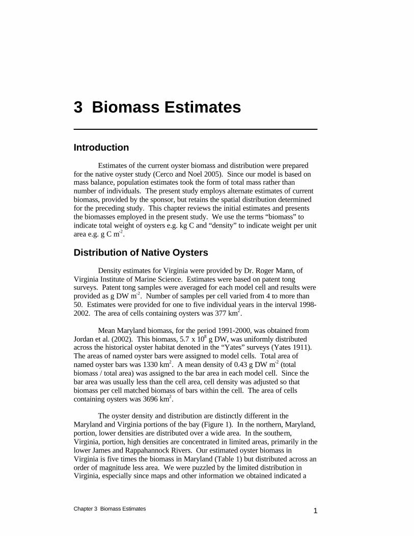
The rate of basal metabolism depends on organism biomass (Winter 1978, Shumway and Koehn 1982). The average oyster in Jordan’s (1987) experiments, upon which our filtration rates are based, is 2.1 g DW. Allometric relationships (Shumway and Koehn 1982) indicate basal metabolism for a 2.1 g DW oyster at 20 oC is 0.002 to 0.005 d-1, depending on salinity. A graphical summary presented by Winter (1978) indicates metabolic rate for a 2 g DW oyster at 20 oC is 0.009 d-1. Winter noted a 1 g DW mussel requires 1.5% of its dry tissue weight daily as a maintenance ration. Based on these reports, the value 0.008 d-1 was employed for basal metabolism at a reference temperature of 20 oC. Parameter KTbmr was assigned the value 0.069 oC-1, equivalent to a Q10 of 2, typical of measured rates in oysters (Shumway and Koehn 1982). The respiratory fraction was assigned through comparison of computed oxygen consumption with metabolism in active oyster reefs (Boucher and Boucher-Rodoni 1988, Dame et al. 1992). The value RF = 0.1 was determined. A comparable value of 0.172 (specific dynamic activity coefficient) was assigned to herbivorous fish in Chesapeake Bay (Luo et al. 2001). Mortality The model considers two forms of mortality. These are mortality due to hypoxia and a term that considers all other sources of mortality including disease and harvest. Although bivalves incorporate physiological responses that render them tolerant to hypoxia, extended periods of anoxia result in near-extinction (Holland et al. 1977, Josefson and Widbom 1988). Casting the results of experiments and observations into a relationship that quantitatively relates mortality to dissolved oxygen concentration incorporates a good deal of uncertainty in functional form and parameterization. The effect of hypoxia on oyster mortality, adopted from the benthos model, employs two concepts. The first is the time to death under complete anoxia. This time to death is converted to a first-order mortality rate via the relationship:
ttdhmr
)100/1ln(= (8)
in which: hmr = mortality due to hypoxia (d-1) ttd = time to death for 99% of the population (14 d)
The mitigating effect on mortality of dissolved oxygen concentration greater than zero is quantified through multiplication by (1 – f(DO)) in which f(DO) is the logistic function that expresses the effects of hypoxia on filtration rate (Equation 6). This functionality increases mortality as dissolved oxygen concentrations become low enough to affect filtration rate (Figure 6). When dissolved oxygen is depleted, filtration rate approaches zero and mortality is at its
Chapter 2 The Oyster Model 8
maximum. As parameterized in the model, effects on filtration and mortality are negligible until dissolved oxygen falls below ˜ 2 g m-3 (Figure 6). The time to death for 99% of the population exceeds 90 days when dissolved oxygen exceeds 1.4 g m-3 (Figure 7). Under this scheme, some fraction of the oyster population can survive an entire summer of hypoxia provided dissolved oxygen exceeds 1.4 g m-3. No significant portion of the oyster population will survive summer hypoxia for dissolved oxygen concentrations below 1.4 g m-3.
Mortality from all other sources, primarily disease and harvest, is
represented by a spatially uniform and temporally constant first-order term. Magnitude of the term is specified to produce various system-wide population levels with the model. The order of magnitude can be derived from Jordan et al. (2002) who reported the 1990 total mortality of “market stock” oysters in northern Chesapeake Bay was 0.94 yr-1 (or 0.0026 d-1). Of this total, 0.22 yr-1 (or 0.0006 d-1) was natural mortality. The balance was fishing mortality. Nutrients Model oysters are composed of carbon, nitrogen, and phosphorus in constant ratios. In the original benthos model (HydroQual 2000), the carbon-to-nitrogen mass ratio of bivalves was set at 5.67:1; the phosphorus-to-carbon mass ratio was 45:1. Composition data for bivalves is not abundant. Calculations by Jordan (1987), based on earlier work by Kuenzler (1961) and Newell (1982), yield a carbon-to-nitrogen mass ratio between 4.8:1 and 6.9:1 and a phosphorus-to-carbon mass ratio of 66:1. The nitrogen composition values encompass the value used in the model. The phosphorus composition value differs from the model but no context exists to judge if the difference is significant. The oyster model differs substantially from the original benthos model in the way nutrients are assimilated and processed. In the orig inal model, nutrients are assimilated and excreted in constant ratios equivalent to the oyster composition. If assimilated carbon is in excess relative to assimilated nitrogen or phosphorus, the excess carbon is converted to feces and the bivalves are effectively nutrient limited. Computed bivalve growth is:
[ ]SFCPPassimSFCNNassimCassimG ⋅⋅= ,,min (9) in which: G = bivalve biomass accumulation (g C m-2 d-1) Cassim = carbon assimilation rate (g C m-2 d-1) Nassim = nitrogen assimilation rate (g N m-2 d-1) SFCN = bivalve carbon-to-nitrogen ratio (g C g-1 N) Passim = phosphorus assimilation rate (g P m-2 d-1) SFCP = bivalve carbon-to-nitrogen ratio (g P g-1 N) If the carbon-to-nitrogen ratio in assimilated food, Cassim/Nassim, exceeds the ratio in bivalve composition, SFCN, then biomass accumulation is proportional to the rate of nitrogen assimilation. Similarly, when the ratio Cassim/Passim > SFCP, biomass accumulation is proportional to phosphorus assimilation. The
Chapter 2 The Oyster Model 9
algal phosphorus-to-carbon ratio in the eutrophication model (Cerco and Noel 2004) is 57:1 for spring diatoms and 80:1 for other algae. Since these ratios exceed SFCP, growth of bivalves feeding on algae will be limited by the phosphorus content of the algae rather than the amount of carbon assimilated. Algal composition does not provide a complete picture of the tendency for nutrient limitation of bivalve growth since modeled bivalves utilize detritus as well as algae. Initial applications of the oyster model indicated, however, that phosphorus limitation of oyster growth did occur. Nutrient limitation was eliminated through two methods. First, oyster phosphorus composition was thinned out; carbon-to-phosphorus ratio was increased to 90:1. More significantly, a mass balance approach to nutrient utilization and excretion was adopted. Biomass accumulation was modeled as carbon assimilation less respiration loss while nutrient excretion was calculated as the amount of assimilated nutrients not required for biomass accumulation. Model Parameters Parameter values for the oyster model are summarized in Table 1.

Chapter 2 The Oyster Model 10
Table 1 Parameters for Oyster Model Parameter Definition Value Units
Frmax maximum filtration rate 0.55 m3 g-1 oyster carbon d-1
Topt optimum temperature for filtration 27 oC
Ktg constant that controls temperature dependence of filtration
0.015 oC-2
KHsoy salinity at which filtration rate is halved 7.5 ppt
BMR base metabolism rate at 20 oC 0.008 d-1
KTbmr constant that controls temperature dependence of metabolism 0.069 oC-1
Tr reference temperature for specification of metabolism 20 oC
RF respiratory fraction 0.1 0 < RF < 1
DOhx dissolved oxygen concentration at which value of logistic function is one-half
1.0 g m-3
DOqx dissolved oxygen concentration at which value of logistic function is one-quarter
0.7 g m-3
ttd time to death for 99% of the population 14 d
aalg assimilation efficiency for phytoplankton 0.75 0 < a < 1
alab assimilation efficiency for labile organic matter 0.75 0 < a < 1
aref assimilation efficiency for refractory organic matter 0.0 0 < a < 1
Imax maximum ingestion rate 0.12 g prey C g-1 C d-1
SFCN carbon-to-nitrogen ratio 6 g C g-1 N
SFCP carbon-to-phosphorus ratio 90 g C g-1 P

Chapter 2 The Oyster Model 11
References Boucher, G., and Boucher-Rodoni, R. (1988). “In situ measurement of
respiratory metabolism and nitrogen fluxes at the interface of oyster beds,” Marine Ecology Progress Series, 44, 229-238.
Cerco, C., and Meyers, M. (2000). “Tributary refinements to the Chesapeake Bay
Model,” Journal of Environmental Engineering, 126(2), 164-174. Cerco, C., Johnson, B., and Wang, H. (2002). “Tributary refinements to the
Chesapeake Bay model, ERDC TR-02-4, US Army Engineer Research and Development Center, Vicksburg, MS.
Cerco, C., and Noel, M. (2004). “The 2002 Chesapeake Bay eutrophication
model,” EPA 903-R-04-004, Chesapeake Bay Program Office, US Environmental Protection Agency, Annapolis, MD.
Cognie, B., Barille, L., and Rince, Y. (2001). “Selective feeding of the oyster
Crassostrea gigas fed on a natural microphytobenthos assemblage,” Estuaries, 24(1), 126-131.
Dame, R., (1972). “Comparison of various allometric relationships in intertidal
and subtidal American oysters,” Fishery Bulletin, 70(4), 1121-1126. Dame, R., Spurrier, J., and Zingmark, R. (1992). “In situ metabolism of an oyster
reef,” Journal of Experimental Marine Biology and Ecology, 164, 147-159.
Dauer, D., Rodi, A., and Ranasinghe, J. (1992). “Effects of low dissolved oxygen
events on the macrobenthos of the lower Chesapeake Bay,” Estuaries, 15(3), 384-391.
DiToro, D. (2001). Sediment Flux Modeling, John Wiley and Sons, New York. Doering, P., and Oviatt, C. (1986). “Application of filtration rate models to field
populations of bivalves: an assessment using experimental mesocosms,” Marine Ecology Progress Series, 31, 265-275.
Doering, P., Oviatt, C., and Kelly, J. (1986). “The effects of the filter-feeding
clam Mercenaria mercenaria on carbon cycling in experimental ecosystems,” Journal of Marine Research, 44, 839-861.
Epifanio, C., and Ewart, J. (1977). “Maximum ration of four algal diets for the
oyster Crassostrea virginica Gmelin,” Aquaculture, 11, 13-29. Hewett, S., and Johnson, B. (1997). “A generalized bioenergetics model of fish
growth for microcomputers,” WIS-SG-87-245, Wisconsin Sea Grant College Program, University of Wisconsin, Madison.
Chapter 2 The Oyster Model 12
Holland, A., Mountford, N., and Mihursky, J. (1977). “Temporal variation in upper bay mesohaline benthic communities: I. The 9-m mud habitat,” Chesapeake Science, 18(4), 370-378.
HydroQual. (2000). “Development of a suspension feeding and deposit feeding
benthos model for Chesapeake Bay,” produced by HydroQual Inc. under contract to the U.S. Army Engineer Research and Development Center, Vicksburg MS.
Jordan, S. (1987). “Sedimentation and remineralization associated with
biodeposition by the American oyster Crassostrea virginica (Gmelin),” Ph.D. diss., University of Maryland, College Park.
Jordan, S., Greenhawk, K., McCollough, C., Vanisko, J., and Homer, M. (2002).
“Oyster biomass, abundance, and harvest in northern Chesapeake Bay: Trends and forecasts,” Journal of Shellfish Research, 21(2), 733-741.
Josefson, A., and Widbom, B. (1988). “Differential response of benthic
macrofauna and meiofauna to hypoxia in the Gullmar Fjord Basin,” Marine Biology, 100, 31-40.
Kuenzler, E. (1961). “Phosphorus budget of a mussel population,” Limnology
and Oceanography, 6, 400-415. Langdon, C., and Newell, R. (1990). “Utilization of detritus and bacteria as food
sources by two bivalve suspension-feeders, the oyster Crassostrea virginica and the mussel Geukensia demissa,” Marine Ecology Progress Series, 58, 299-310.
Loosanoff, V., and Tommers, F. (1948). “Effect of suspended silt and other
substances on rate of feeding of oysters,” Science, 107, 69-70. Loosanoff, V. (1953). “Behavior of oysters in water of low salinities,”
Proceedings of the National Shellfish Association, 43:135-151. Luo, J., Hartman, K., Brandt, S., Cerco, C., and Rippetoe, T. (2001). “A
spatially-explicit approach for estimating carrying capacity: An application for the Atlantic menhaden (Brevoortia tyrannus) in Chesapeake Bay,” Estuaries, 24(4), 545-556.
Meyers, M., DiToro, D., and Lowe, S. (2000). “Coupling suspension feeders to
the Chesapeake Bay eutrophication model,” Water Quality and Ecosystem Modeling, 1, 123-140.
Nestlerode, J., and Diaz, R. (1998). “Effects of periodic environmental hypoxia
on predation of a tethered ploychaete, Glycera Americana: implications for trophic dynamics,” Marine Ecology Progress Series, 172, 185-195.
Newell, R. (1982). “An evaluation of the wet oxidation technique for use in
determining the energy content of seston samples,” Canadian Journal of Fisheries and Aquatic Science, 39, 1383-1388.
Chapter 2 The Oyster Model 13
Newell, R., and Koch, E. (2004). “Modeling seagrass density and distribution in
response to changes in turbidity stemming from bivalve filtration and seagrass sediment stabilization,” Estuaries, 27(5), 793-806.
Riisgard, H. (1988). “Eficiency of particle retention and filtration rate in 6
species of Northeast American bivalves,” Marine Ecology Progress Series, 45, 217-223.
Shumway, S., and Koehn, R. (1982). “Oxygen consumption in the American
oyster Crassostrea virginica,” Marine Ecology Progress Series, 9, 59-68. Steele, J., and Mullin, M. (1977). “Zooplankton dynamics.” The sea. E.
Goldberg, I. McCave, J. O’Brien, J. Steele eds., Volume 6, Wiley-Interscience, New York, 857-890.
Tenore, K., and Dunstan, W. (1973). “Comparison of feeding and biodeposition
of three bivalves at different food levels,” Marine Biology, 21, 190-195. Westrich, J., and Berner, R. (1984). “The role of sedimentary organic matter in
bacterial sulfate reduction: The G model tested,” Limnology and Oceanography, 29, 236-249.
Winter, J. (1978). “A review of the knowledge of suspension-feeding in
lamellibranchiate bivalves, with special reference to artificial aquaculture systems,” Aquaculture, 13, 1-33.
Chapter 2 The Oyster Model 14
Figure 1. Benthos model schematic.
Figure 2. Processes affecting filtered material.
Chapter 2 The Oyster Model 15
Figure 3. Effect of Temperature on filtration rate.
Figure 4. Effect of suspended solids on filtration rate.

Chapter 2 The Oyster Model 16
Figure 5. Effect of salinity on filtration rate.
Figure 6. Effect of dissolved oxygen on filtration and mortality rates.
Chapter 2 The Oyster Model 17
Figure 7. Effect of dissolved oxygen on time to death for 99% of population.
Chapter 3 Biomass Estimates 1
3 Biomass Estimates
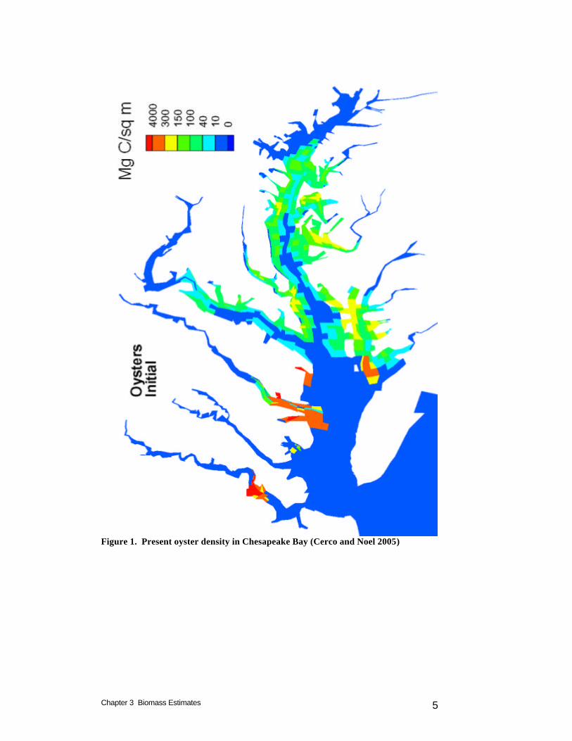
Introduction Estimates of the current oyster biomass and distribution were prepared for the native oyster study (Cerco and Noel 2005). Since our model is based on mass balance, population estimates took the form of total mass rather than number of individuals. The present study employs alternate estimates of current biomass, provided by the sponsor, but retains the spatial distribution determined for the preceding study. This chapter reviews the initial estimates and presents the biomasses employed in the present study. We use the terms “biomass” to indicate total weight of oysters e.g. kg C and “density” to indicate weight per unit area e.g. g C m-2. Distribution of Native Oysters Density estimates for Virginia were provided by Dr. Roger Mann, of Virginia Institute of Marine Science. Estimates were based on patent tong surveys. Patent tong samples were averaged for each model cell and results were provided as g DW m-2. Number of samples per cell varied from 4 to more than 50. Estimates were provided for one to five individual years in the interval 1998-2002. The area of cells containing oysters was 377 km2. Mean Maryland biomass, for the period 1991-2000, was obtained from Jordan et al. (2002). This biomass, 5.7 x 10⁸ g DW, was uniformly distributed across the historical oyster habitat denoted in the “Yates” surveys (Yates 1911). The areas of named oyster bars were assigned to model cells. Total area of named oyster bars was 1330 km2. A mean density of 0.43 g DW m-2 (total biomass / total area) was assigned to the bar area in each model cell. Since the bar area was usually less than the cell area, cell density was adjusted so that biomass per cell matched biomass of bars within the cell. The area of cells containing oysters was 3696 km2. The oyster density and distribution are distinctly different in the Maryland and Virginia portions of the bay (Figure 1). In the northern, Maryland, portion, lower densities are distributed over a wide area. In the southern, Virginia, portion, high densities are concentrated in limited areas, primarily in the lower James and Rappahannock Rivers. Our estimated oyster biomass in Virginia is five times the biomass in Maryland (Table 1) but distributed across an order of magnitude less area. We were puzzled by the limited distribution in Virginia, especially since maps and other information we obtained indicated a
Chapter 3 Biomass Estimates 2
wider distribution of lease holdings and restoration areas. We were assured by Dr. Roger Mann that much of the leased area is unproductive and that biomass outside the areas reported to us is negligible.
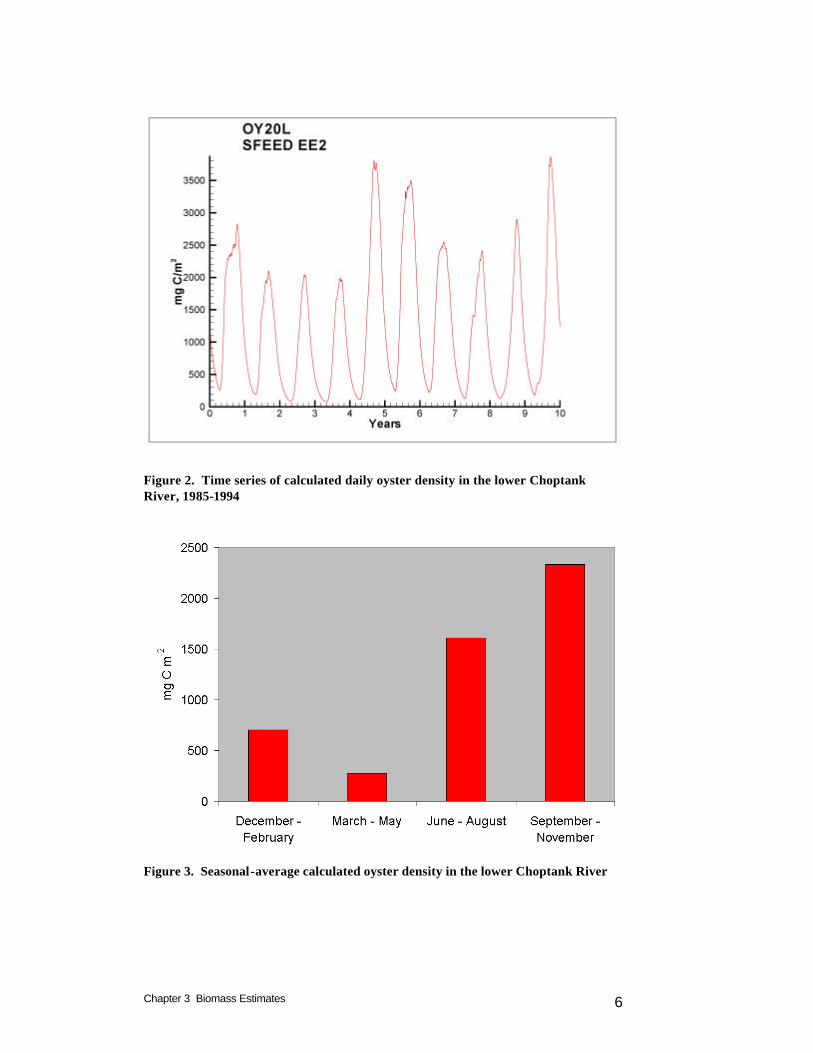
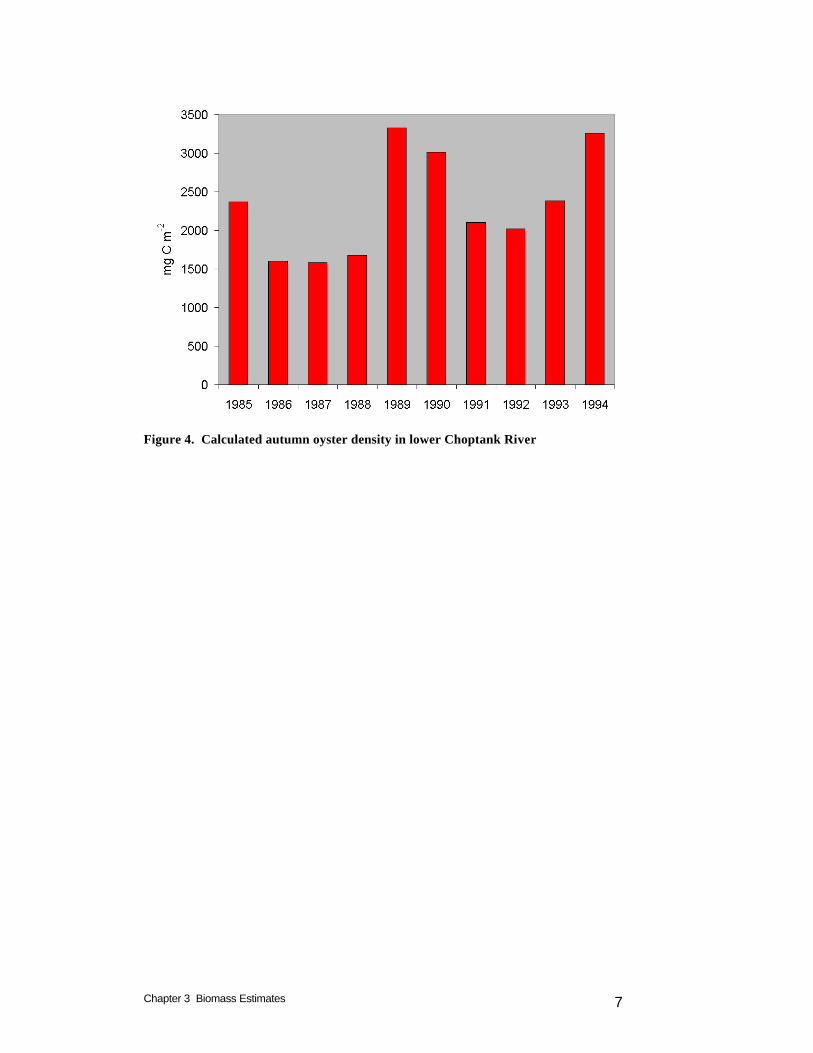
Although the leased area is unproductive, information provided by the sponsor, attributed to the Virginia Marine Resources Commission, indicates 30% of the leased bottom is suitable for larval settling. This suitable area, 84 km2 (20,866 acres), is significant relative to the area of public oyster bars that presently support oysters, 46 km2 (11,366 acres). Model scenarios that consider oyster restoration in portions of Virginia lease holdings and restoration areas would be a worthwhile addition to the scenarios considered thus far. Modeled Biomass Computed density and biomass vary on intra-annual and inter-annual bases (Figure 2). Variations within the annual cycle are largely driven by temperature. Highest densities are computed in late summer and in fall, after a season of filtering at peak rates (Figure 3). Variations from year to year (Figure 4) are largely driven by runoff. Variations in runoff may enhance or diminish computed biomass, depending on local factors. Years with high runoff coincide with large nutrient loads that result in high phytoplankton abundance. The advantages produced by abundant food may be offset, however, by increased anoxia and by sub-optimal salinity.
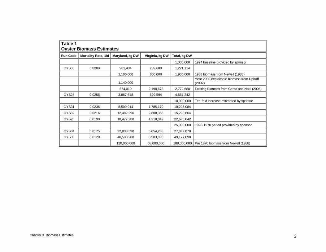
Target values for baywide total biomass were provided by the sponsor. These were approximately matched during the model simulations (Table 1). Exact matching is not possible due to the intra-annual and inter-annual variability. We initially attempted to calculate target oyster densities through dynamic variation of the mortality function. Mortality in each model cell was adjusted upwards or downwards as calculated density exceeded or fell below specified levels. This process ensured that target density was not exceeded but in many cells target density could not be achieved. The problem originated with the attempt to calculate target densities within individual cells. The calculated conditions in many cells would not support the target densities. Consequently, we switched to a strategy in which a bay-wide target biomass was specified. A uniform bay-wide mortality rate was prescribed that produced the target biomass. The mortality rate was obtained through a trial-and-error process in which various rates were prescribed and the calculated biomass was examined. Autumn is the season when individual oysters attain maximum biomass and when most population surveys are conducted. Modeled biomasses reported here (Table 1) are the average calculated autumn (September – November) biomass from ten years (1985 – 1994). The modeled biomasses are interspersed with estimates from various sources. Model run OYS30 is in close agreement with the sponsor’s 1994 baseline estimate. Run OYS31 corresponds to a ten-fold increase over the sponsor’s 1994 baseline. Runs OYS28 and OYS34 bracket the sponsor’s estimate for the 1920-1970 period. The run with the highest calculated biomass, OYS33, represents only 25% of the pre-1870 biomass, however.
Chapter 3 Biomass Estimates 3
Table 1 Oyster Biomass Estimates
Run Code Mortality Rate, 1/d Maryland, kg DW Virginia, kg DW Total, kg DW
1,000,000 1994 baseline provided by sponsor
OYS30 0.0280 981,434 239,680 1,221,114
1,100,000 800,000 1,900,000 1988 biomass from Newell (1988)
1,140,000 Year 2000 exploitable biomass from Uphoff (2002)
574,010 2,198,678 2,772,688 Existing Biomass from Cerco and Noel (2005)
OYS26 0.0255 3,867,648 699,594 4,567,242
10,000,000 Ten-fold increase estimated by sponsor
OYS31 0.0236 8,509,914 1,785,170 10,295,084
OYS32 0.0216 12,482,296 2,808,368 15,290,664
OYS28 0.0190 18,477,200 4,218,842 22,696,042
25,000,000 1920-1970 period provided by sponsor
OYS34 0.0175 22,838,590 5,054,288 27,892,878
OYS33 0.0120 40,593,208 8,583,890 49,177,098
120,000,000 68,000,000 188,000,000 Pre 1870 biomass from Newell (1988)
Chapter 3 Biomass Estimates 4
References Cerco, C., and Noel, M. (2005). “Assessing a ten-fold increase in the Chesapeake
Bay native oyster population,” Chesapeake Bay Program Office, US Environmental Protection Agency, Annapolis, MD. (available at http://www.chesapeakebay.net/modsc.htm)
Jordan, S., Greenhawk, K., McCollough, C., Vanisko, J., and Homer, M. (2002).
“Oyster biomass, abundance, and harvest in northern Chesapeake Bay: Trends and forecasts,” Journal of Shellfish Research, 21(2), 733-741.
Newell, R. (1988). “Ecological changes in Chesapeake Bay: Are they the result
of overharvesting the American oyster (Crassostrea virginica)?,” Understanding the estuary – Advances in Chesapeake Bay Research. Publication 129, Chesapeake Research Consortium, Baltimore, 536-546.
Uphoff, J. (2002). “Biomass dynamic modeling of oysters in Maryland,”
Maryland Department of Natural Resources, Annapolis. (Unpublished manuscript provided by the author).
Yates, C. (1911). “Survey of the oyster bars by county of the State of Maryland,”
Department of Commerce and Labor, Coast and Geodetic Survey, Washington DC.
Chapter 3 Biomass Estimates 5
Figure 1. Present oyster density in Chesapeake Bay (Cerco and Noel 2005)
Chapter 3 Biomass Estimates 6
Figure 2. Time series of calculated daily oyster density in the lower Choptank River, 1985-1994
Figure 3. Seasonal-average calculated oyster density in the lower Choptank River
Chapter 3 Biomass Estimates 7
Figure 4. Calculated autumn oyster density in lower Choptank River
Chapter 4 Ecosystem Services 1
4 Ecoystem Services Provided by Oyster Restoration
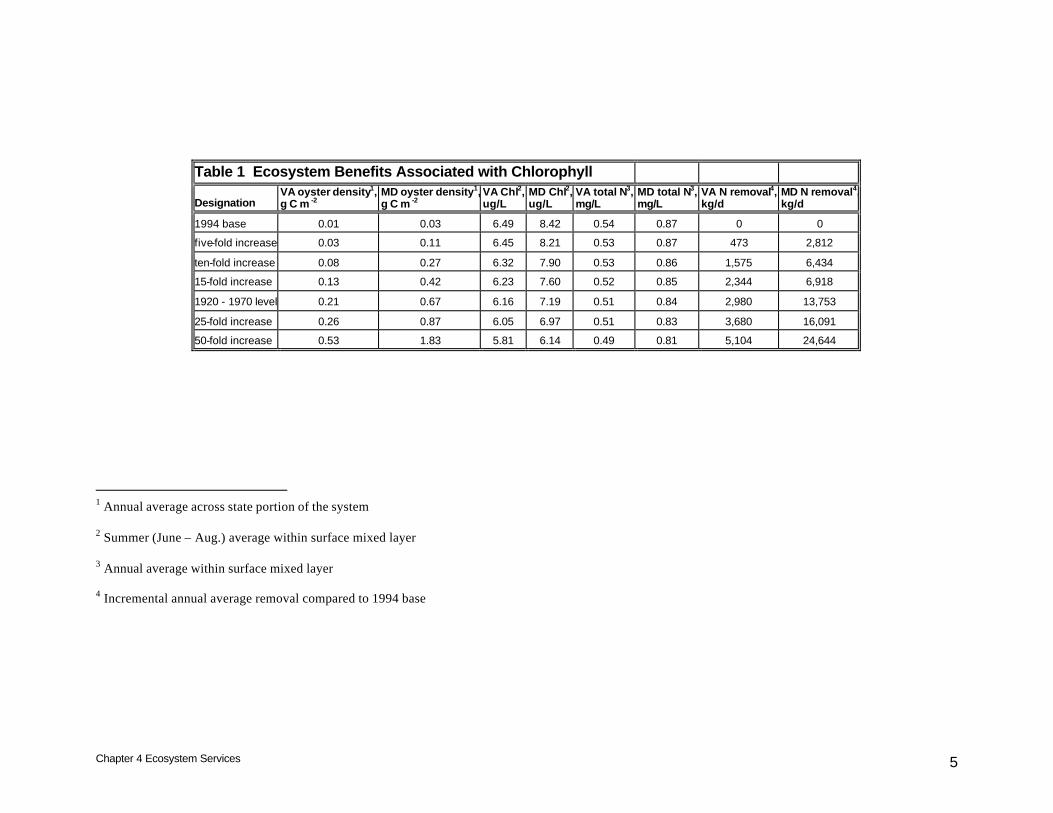
Introduction Oyster restoration can provide a variety of benefits classified under the heading “ecosystem services.” Water quality standards for Chesapeake Bay are based on dissolved oxygen, chlorophyll, and water clarity (U.S. Environmental Protection Agency 2003). Ecosystem services described here are focused on improvements in the water quality standards. Oysters affect their environment on multiple spatial scales ranging from the oyster reef outwards to the entire system. Examinations of oyster impacts on local, regional, and system-wide scales were conducted as part of the study of native oyster restoration (Cerco and Noel 2005). Analyses here divide the bay into two states, Maryland and Virginia. This division was prompted by the sponsor’s request for an estimation of nitrogen removal by state. Chlorophyll Oysters effect improvements in the environment by filtering phytoplankton and other suspended solids from the water column. Aside from direct removal, reductions in phytoplankton, quantified as chlorophyll concentration, may also occur via an indirect process: nutrient limitation induced through removal of nutrients, primarily nitrogen. Although phytoplankton require phosphorus and silica (for diatoms) as well, nitrogen limitation is the most significant influence on algal production in the interval when temperature-dependent oyster filtration is greatest (Fisher et al. 1992, Malone et al. 1996). Within Virginia, the range of densities investigated reduce summer-average surface chlorophyll by up to ˜ 0.7 µg/L, roughly 10% of the 1994 base concentration (Table 1). Corresponding reductions in Maryland are up to ˜ 2.3 µg/L, more than 25% of the 1994 base. The disparity between the two states reflects the widespread distribution of oysters in Maryland relative to Virginia. Averaged over the area contained within each state, oyster densities are three to four times greater in Maryland than Virginia for any level or restoration (Table 1). The range of densities investigated reduced surface total nitrogen concentration by up to 0.05 mg/L in Virginia (Table 1). The maximum reduction
Chapter 4 Ecosystem Services 2
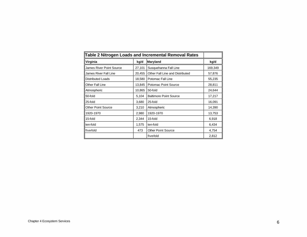
was nearly identical in Maryland, 0.06 mg/L. Under base conditions, net nitrogen removal in Maryland, on an areal basis, is greater than in Virginia, 27 mg N m-2d-1 versus 16 mg N m-2 d-1. The higher base rate in Maryland reflects deposition of particulate nitrogen below the major fall lines and diffusion of nitrate into bed sediments where it is subsequently denitrified. The difference between the two regions increases with the level of oyster restoration, attributable to the higher densities in Maryland. At the greatest densities examined, oyster restoration removes 4 mg N m-2 d-1 in Maryland versus 1 mg N m-2 d-1 in Virginia. Multiplication by bottom area in each state yields removal rate in mass terms: up to 24,600 kg d-1 additional nitrogen removal in Maryland versus up to 5,100 kg d-1 additional removal in Virginia (Table 1). These removal rates can be put in perspective by examining some of the other loads to the system, derived from the 2002 model used for the recent load allocations (Cerco and Noel 2004). The Maryland removal rate corresponding to a fifty-fold increase in oyster biomass is roughly equivalent to the point-source nitrogen load to the Potomac basin (Table 2). The equivalence in loading should not be extended to equivalence in effects, however since the majority of the Potomac load enters in the tidal freshwater reach far removed from oyster habitat. The amount of nitrogen removed by Maryland oyster restoration to 1920 – 1970 levels is equivalent to direct atmospheric loading to the water surface; nitrogen removal from a ten-fold oyster restoration is half this amount. The Virginia removal rate corresponding to a fifty-fold increase in oyster biomass is only half of direct atmospheric loading to the water surface (Table 2). Removal rates associated with restoration of oysters to 1920 – 1970 levels and with ten-fold oyster restoration are only small fractions of identifiable loads to the Virginia portion of the bay. Additional perspective is gained by comparing the nitrogen removal via oyster restoration to nutrient reduction targets (Linker 2005). Recent allocations call for a 24,900 kg d-1 reduction in Maryland nitrogen loading. The allocation corresponds to nitrogen removal from a fifty-fold increase in oyster biomass (Table 2). The Virginia allocation calls for a 34,800 kg d-1 reduction in nitrogen loading. This allocation exceeds any feasible reduction from oyster restoration. The system-wide allocation calls for a 124,500 kg d-1 reduction in nitrogen loading. This allocation also exceeds any feasible reduction from oyster restoration. Nitrogen removal via oyster restoration can be a valuable supplement to alternate methods of nutrient control but is no substitute for conventional nutrient controls. Dissolved Oxygen Bottom-water hypoxia originates with excess algal production in the surface waters of the bay. Algae and detritus settle to the bottom where they undergo decay that generates oxygen demand and consumption. Density stratification prevents replenishment of oxygen-depleted waters with atmospheric oxygen from the surface.
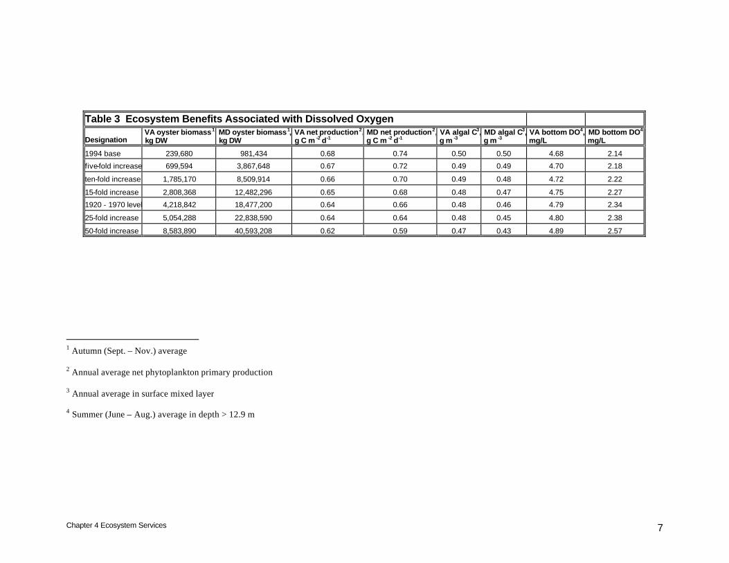
Chapter 4 Ecosystem Services 3
Within Virginia, the range of oyster densities investigated reduced annual-average net algal production by up to 10%, from 0.68 g C m-2 d-1 at base levels to 0.62 g C m-2 d-1, for a fifty-fold increase in oyster biomass (Table 3). Corresponding reductions were greater in Maryland. Annual average net algal production was reduced up to 20%, from 0.74 g C m-2 d-1 at base levels to 0.59 g C m-2 d-1, for a fifty-fold increase in oyster biomass. Under base conditions, annual-average surface algal carbon concentration was equivalent in Maryland and Virginia, 0.5 g C m-3 (Table 3). The maximum potential reduction attainable in Maryland, 0.07 g C m-3, was double the potential gain in Virginia, however. Oxygen improvements are considered for summer-average at depths greater than 12.9 m. This period and depth isolates the time and location of bottom-water hypoxia. Within Virginia, the improvement in bottom-water dissolved oxygen at the maximum biomass investigated was 0.2 mg/L (Table 3). Within Maryland, the improvement was doubled, more than 0.4 mg/L. Water Clarity Improvements in water clarity are effected by removal of both organic and inorganic solids from the water column. Water clarity is quantified in the model as the coefficient of diffuse light attenuation. The light attenuation coefficient is inversely proportional to water clarity. Lower light attenuation implies higher water clarity. We examined summer-average light attenuation since summer is the critical period for growth of submerged aquatic vegetation (SAV).
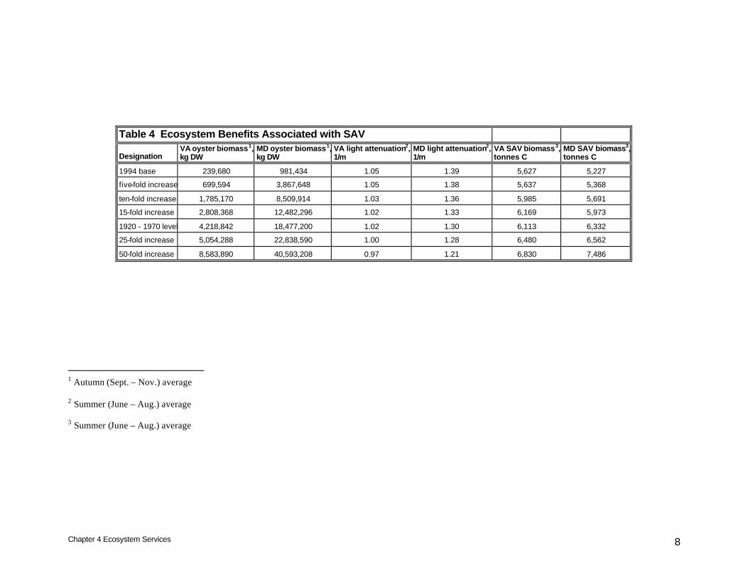
Within Virginia, the range of oyster densities investigated reduced summer-average light attenuation by up to 8%, from 1.05 m-1 at base levels to 0.97 m-1 for a fifty-fold increase in oyster biomass (Table 4). Percentage increases in summer SAV biomass were greater, up to 21%. Computed SAV biomass increased from 5,627 tonnes C under base conditions to 6,830 tonnes for a fifty-fold oyster restoration. Following a pattern established for other benefits, improvements in Maryland exceeded Virginia. Summer-average light attenuation diminished by up to 13%, from 1.39 m-1 under base conditions to 1.21 m-1 for a fifty-fold increase in oyster biomass. Corresponding percentage improvements in SAV, up to 43%, again exceeded improvements in attenuation. Computed summer SAV biomass increased from 5,227 tonnes C under base conditions to 7,486 tonnes C under maximum restoration. Discussion Results from these model runs were compared to runs conducted for the native oyster study (Cerco and Noel 2005). Results from all runs form a consistent body when compared on identical spatial scales e.g. model cell or system-wide. The reader is cautioned regarding nomenclature, however. Results from both studies were reported based on various levels of restoration including existing, ten-fold restoration, and historic levels. The existing oyster biomass provided by the sponsor of this study is less than the existing biomass derived by us for the native oyster study (Chapter 3, Table 1). Consequently , the ten-fold increase computed in this study represents lower biomass than the ten-fold
Chapter 4 Ecosystem Services 4
increase computed for the native oyster study. In the native oyster study, historical biomass refers to pre-1870 levels while the sponsor of this study uses “historical” to represent the 1920 – 1970 period. We recommend that results from both studies be summarized on identical spatial scales and presented as a function of target biomass rather than restoration levels. Our work indicates the maximum improvement expected in deep-water summer dissolved oxygen is 0.2 (Virginia) to 0.4 (Maryland) mg/L. These effects are averaged over large expanses of the bay. Greater and lesser improvements will be found in specific locations. Still, oyster restoration alone is not likely to bring the deep channel of the mainstem, where complete anoxia may occur, into compliance with dissolved oxygen standards. Multiple reasons can be offered for the absence of more significant dissolved oxygen response to oyster restoration. The obvious explanation is that oysters are found in the shoals rather than over the deep trench. Phytoplankton production over the trench remains free to settle to bottom waters and contribute to anoxia. A more subtle explanation lies in the origins of mainstem anoxia. Oxygen depletion in the upper bay does not originate solely with excess production in the overlying waters. Rather, oxygen depletion is accumulated as net circulation moves bottom water up the channel from the mouth of the bay. This mechanism was originally proposed by Kuo et al. (1991) for the Rappahannock River and has been shown to apply to the mainstem bay as well (Cerco 1995). Improvement in upper bay dissolved oxygen requires reduction in lower bay oxygen demand. Oysters in the lower bay are concentrated in the western-shore tributaries, however. The oyster restoration strategy does little to diminish oxygen demand in the lower bay and, consequently, has limited impact on the upper bay.
Our model provides unique capability to address oyster restoration in the bay. We believe ours is the first approach to combine detailed representation of the bay geometry with mechanistic representations of three-dimensional transport, water-column eutrophication processes, sediment diagenetic processes, and dynamic computation of oyster biomass. Due to the large number of computed interactions, exact quantification of benefits such as SAV biomass improvement involves uncertainty. We believe, however, our basic findings regarding the nature and magnitude of restoration benefits are valid. Our results are consistent with the earlier findings of Officer et al (1992) and Gerritson et al. (1994) and with the recent findings of Newell and Koch (2004). Benthic controls of algal production are most effective in shallow, spatially-limited regions. In these shallow regions, oyster removal of solids from the water column enhances adjacent SAV beds. The ability to influence deep regions of large spatial extent is limited by the location of oysters in the shoals and by exchange processes between the shoals and deeper regions. We recommend that oyster restoration be targeted to specific areas with suitable environments and that resulting environmental improvements be viewed on similar, local scales.
Chapter 4 Ecosystem Services 5
Table 1 Ecosystem Benefits Associated with Chlorophyll
Designation VA oyster density1, g C m -2
MD oyster density1, g C m -2
VA Chl2, ug/L
MD Chl2, ug/L
VA total N3, mg/L
MD total N3, mg/L
VA N removal4, kg/d
MD N removal4, kg/d
1994 base 0.01 0.03 6.49 8.42 0.54 0.87 0 0
five-fold increase 0.03 0.11 6.45 8.21 0.53 0.87 473 2,812
ten-fold increase 0.08 0.27 6.32 7.90 0.53 0.86 1,575 6,434
15-fold increase 0.13 0.42 6.23 7.60 0.52 0.85 2,344 6,918
1920 - 1970 level 0.21 0.67 6.16 7.19 0.51 0.84 2,980 13,753
25-fold increase 0.26 0.87 6.05 6.97 0.51 0.83 3,680 16,091
50-fold increase 0.53 1.83 5.81 6.14 0.49 0.81 5,104 24,644
1 Annual average across state portion of the system 2 Summer (June – Aug.) average within surface mixed layer 3 Annual average within surface mixed layer 4 Incremental annual average removal compared to 1994 base
Chapter 4 Ecosystem Services 6
Table 2 Nitrogen Loads and Incremental Removal Rates
Virginia kg/d Maryland kg/d
James River Point Source 27,101 Susquehanna Fall Line 169,349
James River Fall Line 20,455 Other Fall Line and Distributed 57,876
Distributed Loads 18,580 Potomac Fall Line 55,235
Other Fall Line 13,845 Potomac Point Source 28,811
Atmospheric 10,865 50-fold 24,644
50-fold 5,104 Baltimore Point Source 17,217
25-fold 3,680 25-fold 16,091
Other Point Source 3,210 Atmospheric 14,390
1920-1970 2,980 1920-1970 13,753
15-fold 2,344 15-fold 6,918
ten-fold 1,575 ten-fold 6,434
five-fold 473 Other Point Source 4,754
five-fold 2,812
Chapter 4 Ecosystem Services 7
Table 3 Ecosystem Benefits Associated with Dissolved Oxygen
Designation VA oyster biomass1, kg DW
MD oyster biomass1, kg DW
VA net production2, g C m -2 d-1
MD net production2, g C m -2 d-1
VA algal C3, g m -3
MD algal C3, g m -3
VA bottom DO4, mg/L
MD bottom DO4, mg/L
1994 base 239,680 981,434 0.68 0.74 0.50 0.50 4.68 2.14
five-fold increase 699,594 3,867,648 0.67 0.72 0.49 0.49 4.70 2.18
ten-fold increase 1,785,170 8,509,914 0.66 0.70 0.49 0.48 4.72 2.22
15-fold increase 2,808,368 12,482,296 0.65 0.68 0.48 0.47 4.75 2.27
1920 - 1970 level 4,218,842 18,477,200 0.64 0.66 0.48 0.46 4.79 2.34
25-fold increase 5,054,288 22,838,590 0.64 0.64 0.48 0.45 4.80 2.38
50-fold increase 8,583,890 40,593,208 0.62 0.59 0.47 0.43 4.89 2.57
1 Autumn (Sept. – Nov.) average 2 Annual average net phytoplankton primary production 3 Annual average in surface mixed layer 4 Summer (June – Aug.) average in depth > 12.9 m
Chapter 4 Ecosystem Services 8
Table 4 Ecosystem Benefits Associated with SAV
Designation VA oyster biomass1, kg DW
MD oyster biomass1, kg DW
VA light attenuation2, 1/m
MD light attenuation2, 1/m
VA SAV biomass3, tonnes C
MD SAV biomass3, tonnes C
1994 base 239,680 981,434 1.05 1.39 5,627 5,227
five-fold increase 699,594 3,867,648 1.05 1.38 5,637 5,368
ten-fold increase 1,785,170 8,509,914 1.03 1.36 5,985 5,691
15-fold increase 2,808,368 12,482,296 1.02 1.33 6,169 5,973
1920 - 1970 level 4,218,842 18,477,200 1.02 1.30 6,113 6,332
25-fold increase 5,054,288 22,838,590 1.00 1.28 6,480 6,562
50-fold increase 8,583,890 40,593,208 0.97 1.21 6,830 7,486
1 Autumn (Sept. – Nov.) average 2 Summer (June – Aug.) average 3 Summer (June – Aug.) average
Chapter 4 Ecosystem Services 10
References Cerco, C., and Noel, M. (2005). “Assessing a ten-fold increase in the Chesapeake
Bay native oyster population,” Chesapeake Bay Program Office, US Environmental Protection Agency, Annapolis, MD. (available at http://www.chesapeakebay.net/modsc.htm)
Cerco, C., and Noel, M. (2004). “The 2002 Chesapeake Bay eutrophication
model,” EPA 903-R-04-004, Chesapeake Bay Program Office, US Environmental Protection Agency, Annapolis, MD. (available at http://www.chesapeakebay.net/modsc.htm)
Fisher T, Peele E, Ammerman J, Harding L (1992). Nutrient limitation of
phytoplankton in Chesapeake Bay. Mar Ecol Prog Ser 82:51-63 Gerritsen, J., Holland, A., and Irvine, D. (1994). “Suspension-feeding bivalves
and the fate of primary production: An estuarine model applied to Chesapeake Bay,” Estuaries, 17(2), 403-416.
Kuo, A., Park, K., and Moustafa, Z. (1991). “Spatial and temporal variabilities of
hypoxia in the Rappahannock River, Virginia,” Estuaries, 14(2), 113-121.
Linker, L. (2005). Personal communication. Malone T, Conley D, Fisher T, Glibert P, Harding, Sellner K (1996). Scales of
nutrient-limited phytoplankton productivity in Chesapeake Bay. Estuaries 19:371-385
Newell, R., and Koch, E. (2004). “Modeling seagrass density and distribution in
response to changes in turbidity stemming from bivalve filtration and seagrass sediment stabilization,” Estuaries, 27(5), 793-806.
Officer, C., Smayda, T., and Mann, R. (1982). “Benthic filter feeding: A natural
eutrophication control,” Marine Ecology Progress Series, 9, 203-210. U.S. Environmental Protection Agency. (2003). “Ambient water quality criteria
for dissolved oxygen, water clarity and chlorophyll a for the Chesapeake Bay and its tidal tributaries”, EPA 903-R-03-002, U.S. Environmental Protection Agency Region III Chesapeake Bay Program Office, Annapolis MD. (available at http://www.chesapeakebay.net/baycriteria.htm)
Chapter 5 Info for Risk Assessment 1
5 Information for Risk Assessment
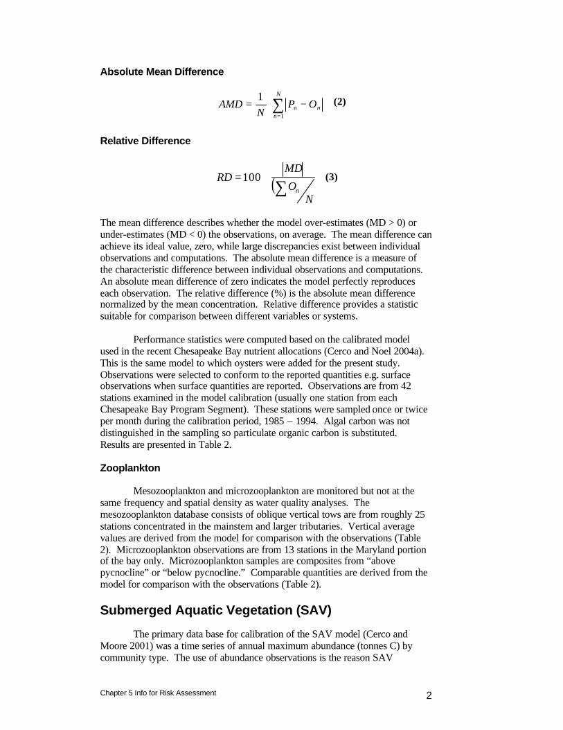
Introduction The project work plan calls for “…a discussion of uncertainty associated with model results and the best available quantitative estimation of uncertainty in results.” The ability to distinguish and quantify uncertainty varies with the nature of the model outputs. The uncertainty in quantities that are directly calculated by the model and regularly observed can be readily quantified. Uncertainty in derived model outputs or in quantities for which insufficient observations are available can be difficult or impossible to quantify although some qualitative description of uncertainty may still be possible. The quantities reported to the sponsor are presented in Table 1. Uncertainty in quantities that are part of the Bay Program monitoring program is quantified using the statistics described below. Uncertainty in the remaining quantities is described based on available information and the modelers’ experience. Statistical Summaries Statistics can be a valuable aid in assessing model performance. A wide variety of statistics is available and no standard suite exists. Neither are there definite criteria available for judging the success of model computations. We use a suite that has been applied to the succession of Chesapeake Bay applications and to other CE-QUAL-ICM applications. Use of these statistics allows for consistent interpretation of model performance and provides a database of comparable statistics from alternate model applications. Our standard statistics are: Mean Difference
(1)
in which: N = number of observations On = nth observation Pn = computation corresponding to nth observation
∑=
−⋅=N
nnOP
NMD
1n )(
1
Chapter 5 Info for Risk Assessment 2
Absolute Mean Difference
(2)
Relative Difference
(3) The mean difference describes whether the model over-estimates (MD > 0) or under-estimates (MD < 0) the observations, on average. The mean difference can achieve its ideal value, zero, while large discrepancies exist between individual observations and computations. The absolute mean difference is a measure of the characteristic difference between individual observations and computations. An absolute mean difference of zero indicates the model perfectly reproduces each observation. The relative difference (%) is the absolute mean difference normalized by the mean concentration. Relative difference provides a statistic suitable for comparison between different variables or systems. Performance statistics were computed based on the calibrated model used in the recent Chesapeake Bay nutrient allocations (Cerco and Noel 2004a). This is the same model to which oysters were added for the present study. Observations were selected to conform to the reported quantities e.g. surface observations when surface quantities are reported. Observations are from 42 stations examined in the model calibration (usually one station from each Chesapeake Bay Program Segment). These stations were sampled once or twice per month during the calibration period, 1985 – 1994. Algal carbon was not distinguished in the sampling so particulate organic carbon is substituted. Results are presented in Table 2. Zooplankton Mesozooplankton and microzooplankton are monitored but not at the same frequency and spatial density as water quality analyses. The mesozooplankton database consists of oblique vertical tows are from roughly 25 stations concentrated in the mainstem and larger tributaries. Vertical average values are derived from the model for comparison with the observations (Table 2). Microzooplankton observations are from 13 stations in the Maryland portion of the bay only. Microzooplankton samples are composites from “above pycnocline” or “below pycnocline.” Comparable quantities are derived from the model for comparison with the observations (Table 2). Submerged Aquatic Vegetation (SAV) The primary data base for calibration of the SAV model (Cerco and Moore 2001) was a time series of annual maximum abundance (tonnes C) by community type. The use of abundance observations is the reason SAV
∑=
−⋅=N
nnOP
NAMD
1n
1
( )N
O
MDRD
n∑⋅=100
Chapter 5 Info for Risk Assessment 3
abundance is the primary quantity reported as model output. The model was also compared to living-resource criteria, primarily light attenuation. The following verbiage was used to describe model performance: “Comparison of model results with time series of observed community abundance indicates the model represents correctly the relative abundance in each community. Inter-annual variability and trends are not well represented, however. The median absolute difference between computed and observed bay-wide annual abundance, by community type, is 30% of observed values, with a range from zero to 240%.” Net Primary Production Development of primary production algorithms was the subject of special emphasis in the present Chesapeake Bay Environmental Model Package (Cerco and Noel 2004b). The model was calibrated against a data base of more than 160 observations collected throughout the bay from 1987 to 1994. Use of a paired t-test to compare individual observations with model calculations indicated the mean difference between computed and observed net production could not be distinguished from zero (p < 0.01). Regression was used to compare individual computations with observations. Results for the regression of computed versus observed net primary production were:
• Slope = 0.57 (95% CI = 0.08) • Intercept = 0.32 (95% CI = 0.10) • R2 = 0.26 • p < 0.0001
Benthic Algae The benthic algae model was developed for the Delaware Inland Bays (Cerco and Seitzinger 1997) and adapted to the Chesapeake Bay (Cerco and Noel 2004a). No local observations of benthic algal biomass exist for comparison with the model. Computed benthic algal biomass, up to 3 g C m-2, was found to be consistent with biomass observed in a variety of systems. The model was checked for consistency with observed properties of benthic algae and their effects. The primary determinant of benthic algae is light at the sediment water interface. Algal density increases or decreases as illumination increases or decreases. We can conclude that algal biomass computed by the model is order-of-magnitude correct and responds correctly to environmental influences. Deposit and Filter Feeding Benthos Benthic deposit feeders and bivalve filter feeders (other than oysters) were added to the model as part of the Virginia Tributaries Refinements phase (HydroQual 2000). Computed benthos were compared to observations collected at various locations throughout the system. Observations showed a large degree of heterogeneity. Variations of two to four orders of magnitude in benthic biomass were commonly observed over the multi-year course of the sampling program. The variability made conventional comparisons of computations and observations (e.g. time series) difficult to evaluate. Probability plots were constructed that compared the distributions of observations and corresponding
Chapter 5 Info for Risk Assessment 4
computations at various sampling stations. Emphasis in evaluation was placed on the median observed and computed values. At some locations, the medians were within a few percent of each other. At other locations median observations and computations were separated by one to two orders of magnitude.
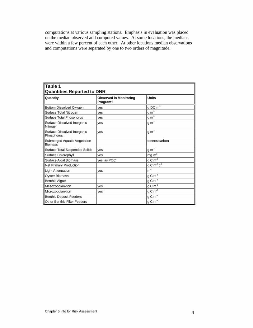
Table 1 Quantities Reported to DNR Quantity Observed in Monitoring
Program? Units
Bottom Dissolved Oxygen yes g DO m-3 Surface Total Nitrogen yes g m-3 Surface Total Phosphorus yes g m-3
Surface Dissolved Inorganic Nitrogen
yes g m-3
Surface Dissolved Inorganic Phosphorus
yes g m-3
Submerged Aquatic Vegetation Biomass
tonnes carbon
Surface Total Suspended Solids yes g m-3
Surface Chlorophyll yes mg m-3
Surface Algal Biomass yes, as POC g C m-3 Net Primary Production g C m-2 d-1
Light Attenuation yes m-1
Oyster Biomass g C m-2 Benthic Algae g C m-2
Mesozooplankton yes g C m-3
Microzooplankton yes g C m-3
Benthic Deposit Feeders g C m-2 Other Benthic Filter Feeders g C m-2
Chapter 5 Info for Risk Assessment 5
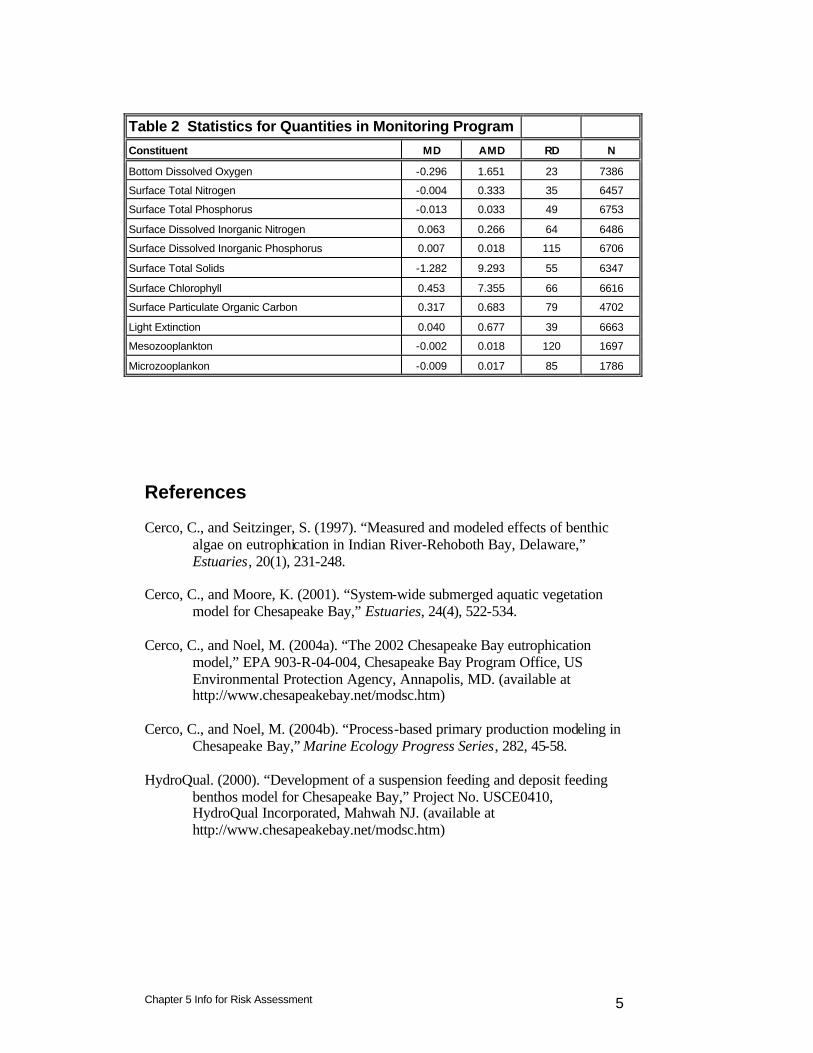
Table 2 Statistics for Quantities in Monitoring Program
Constituent MD AMD RD N
Bottom Dissolved Oxygen -0.296 1.651 23 7386
Surface Total Nitrogen -0.004 0.333 35 6457
Surface Total Phosphorus -0.013 0.033 49 6753
Surface Dissolved Inorganic Nitrogen 0.063 0.266 64 6486
Surface Dissolved Inorganic Phosphorus 0.007 0.018 115 6706
Surface Total Solids -1.282 9.293 55 6347
Surface Chlorophyll 0.453 7.355 66 6616
Surface Particulate Organic Carbon 0.317 0.683 79 4702
Light Extinction 0.040 0.677 39 6663
Mesozooplankton -0.002 0.018 120 1697
Microzooplankon -0.009 0.017 85 1786
References Cerco, C., and Seitzinger, S. (1997). “Measured and modeled effects of benthic
algae on eutrophication in Indian River-Rehoboth Bay, Delaware,” Estuaries, 20(1), 231-248.
Cerco, C., and Moore, K. (2001). “System-wide submerged aquatic vegetation
model for Chesapeake Bay,” Estuaries, 24(4), 522-534. Cerco, C., and Noel, M. (2004a). “The 2002 Chesapeake Bay eutrophication
model,” EPA 903-R-04-004, Chesapeake Bay Program Office, US Environmental Protection Agency, Annapolis, MD. (available at http://www.chesapeakebay.net/modsc.htm)
Cerco, C., and Noel, M. (2004b). “Process-based primary production modeling in
Chesapeake Bay,” Marine Ecology Progress Series, 282, 45-58. HydroQual. (2000). “Development of a suspension feeding and deposit feeding
benthos model for Chesapeake Bay,” Project No. USCE0410, HydroQual Incorporated, Mahwah NJ. (available at http://www.chesapeakebay.net/modsc.htm)
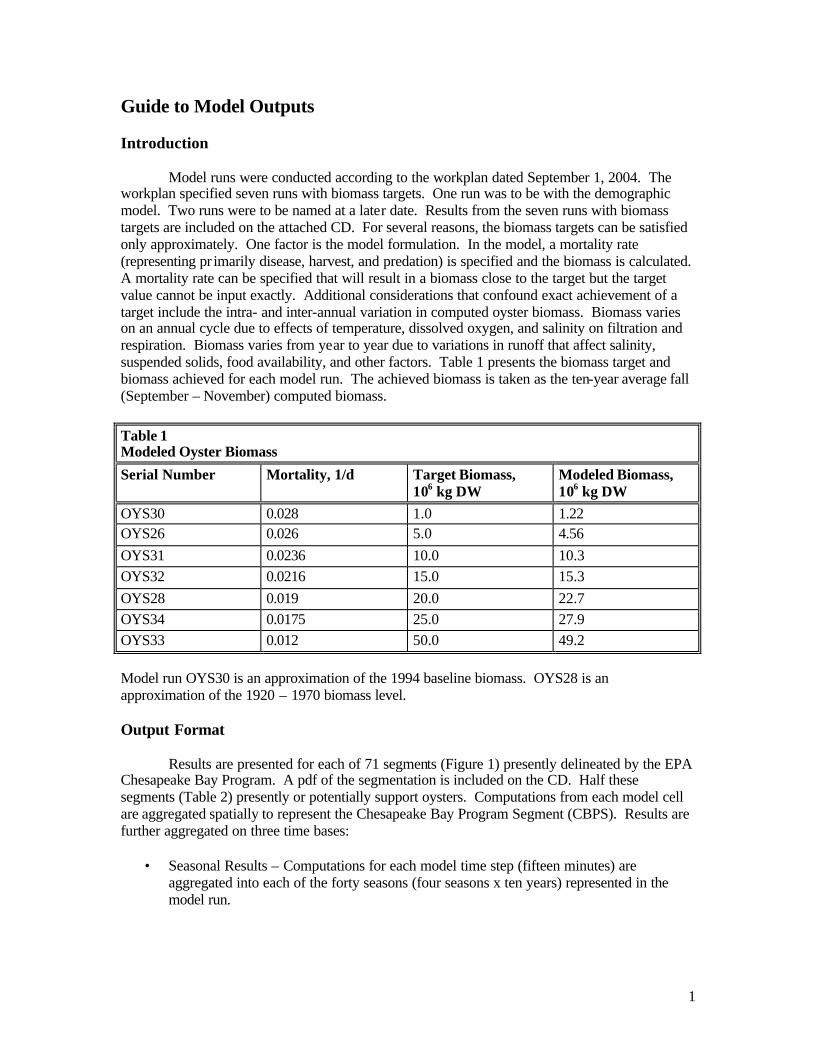
1
Guide to Model Outputs Introduction Model runs were conducted according to the workplan dated September 1, 2004. The workplan specified seven runs with biomass targets. One run was to be with the demographic model. Two runs were to be named at a later date. Results from the seven runs with biomass targets are included on the attached CD. For several reasons, the biomass targets can be satisfied only approximately. One factor is the model formulation. In the model, a mortality rate (representing pr imarily disease, harvest, and predation) is specified and the biomass is calculated. A mortality rate can be specified that will result in a biomass close to the target but the target value cannot be input exactly. Additional considerations that confound exact achievement of a target include the intra- and inter-annual variation in computed oyster biomass. Biomass varies on an annual cycle due to effects of temperature, dissolved oxygen, and salinity on filtration and respiration. Biomass varies from year to year due to variations in runoff that affect salinity, suspended solids, food availability, and other factors. Table 1 presents the biomass target and biomass achieved for each model run. The achieved biomass is taken as the ten-year average fall (September – November) computed biomass.
Table 1 Modeled Oyster Biomass
Serial Number Mortality, 1/d Target Biomass, 106 kg DW
Modeled Biomass, 106 kg DW
OYS30 0.028 1.0 1.22 OYS26 0.026 5.0 4.56 OYS31 0.0236 10.0 10.3 OYS32 0.0216 15.0 15.3 OYS28 0.019 20.0 22.7 OYS34 0.0175 25.0 27.9 OYS33 0.012 50.0 49.2 Model run OYS30 is an approximation of the 1994 baseline biomass. OYS28 is an approximation of the 1920 – 1970 biomass level. Output Format Results are presented for each of 71 segments (Figure 1) presently delineated by the EPA Chesapeake Bay Program. A pdf of the segmentation is included on the CD. Half these segments (Table 2) presently or potentially support oysters. Computations from each model cell are aggregated spatially to represent the Chesapeake Bay Program Segment (CBPS). Results are further aggregated on three time bases:
• Seasonal Results – Computations for each model time step (fifteen minutes) are aggregated into each of the forty seasons (four seasons x ten years) represented in the model run.
2
• Seasonal Averages – Seasonal results are aggregated into four seasons each representing the average of ten computed seasons.
• Annual Averages - Computations for each model time step are aggregated into each of
the ten years represented in the model run.
Table 2 CBPS that Support Oysters BIGMH CHOOH MANMH POTMH CB2OH CHSMH MOBPH POTOH CB3MH CRRMH NANMH RHDMH CB4MH EASMH PATMH RPPMH CB5MH FSBMH PAXMH SEVMH CB6PH HNGMH PAXOH SOUMH CB7PH JMSMH PIAMH TANMH CHOMH1 LCHMH POCMH WICMH CHOMH2 MAGMH POCOH WSTMH
Seasons are defined as follows:
• Winter – December through February • Spring – March through May • Summer – June through August • Fall – September through November
Several reported quantities are most relevant when reported for a specific location in the
water column e.g. surface chlorophyll or bottom dissolved oxygen. In keeping with long-established model convention, “surface” is defined as all model cells within a layer that extends 6.7 m down from the air-water interface. This length scale approximates the surface mixed layer. The definition of “bottom” depends on local depth. For the deepest segments, the bottom includes all model cells greater than 12.8 m down from the air-water interface. Water at this depth is “below pycnocline.” For segments with no cells below 12.8 m, bottom includes all cells greater then 6.7 m down from the air-water interface. For segments with no cells below 6.7 m, bottom includes all cells less than 6.7 m down from the air-water interface and coincides with surface.
Results are provided in graphical and numerical formats on the CD. The CD is divided
into folders that correspond with run serial numbers (Table 1). Within the folders are pdf’s of graphical results and multiple subfolders. The subfolders contain text files of the material presented in graphical format. Each CBPS is represented by two text files. (The use of two files makes these “printer friendly.”) Each column in the file contains a header consisting of a parameter code and the CBPS designation. For the “Seasonal” text files, the column headed “year” represents the decimal years into the model run at which the designated season ends. Reported quantities, parameter codes, and units are presented in Table 3.
3
Table 3 Reported Quantities Quantity Parameter Code Units Bottom Dissolved Oxygen botdo g DO m-3 Surface Total Nitrogen tn g m-3 Surface Total Phosphorus tp g m-3 Surface Dissolved Inorganic Nitrogen
din g m-3
Surface Dissolved Inorganic Phosphorus
dip g m-3
Submerged Aquatic Vegetation Biomass
savbi tonnes carbon
Surface Total Suspended Solids
tss g m-3
Surface Chlorophyll chl mg m-3 Surface Algal Biomass alcar g C m-3 Net Primary Production npp g C m-2 d-1 Light Attenuation ke m-1 Oyster Biomass oys g C m-2 Benthic Algae benal g C m-2 Mesozooplankton meso g C m-3 Microzooplankton micro g C m-3 Benthic Deposit Feeders dfeed g C m-2 Other Benthic Filter Feeders ofeed g C m-2
4
Figure 1. Chesapeake Bay Program Segments