Embed Size (px)
Citation preview

Evaluating Corporate Bonds with Complex Debt
Structure
Dai, Tian-Shyr ∗ Wang, Chuan-Ju † Liu, Liang-Chih ‡
Abstract
Most structural models of credit risk ignore the impacts caused by various properties of out-
standing bonds and may carry out biased analyses against real world phenomena observed by
empirical studies on debt heterogeneity. This paper analyzes the impacts of debt heterogeneity on
the values of corporate securities and issuers’ redemption policies by incorporating the following
four facets of an issuer’s debt structure: the leverage ratio, maturity structure, priority structure
and covenant structure into a structural model. These complex analyses are achieved by construct-
ing a novel quantitative framework, the multi-layer forest, to capture the contingent changes of an
issuer’s capital structure due to certain properties of that issuer’s debt structure, like early redemp-
tion provisions embedded in callable bonds. Our work provides theoretical insights and concrete
quantitative measurements on empirical phenomena, like the shapes of credit spread curves, the
impacts of payment blockage and poison put covenant on other outstanding bonds of the same
issuer, and the call delay phenomenon due to tax shield benefits and wealth transfer effect. This
framework can also be applied to explore new phenomena that are hard to be empirically analyzed
due to lack of data and illiquidity.
Keywords: Debt structure, maturity structure, priority structure, covenant structure, payment
blockage, poison put, call delay
∗Department of Information and Finance Management, Institute of Finance and Institute of Information Manage-ment, National Chiao-Tung University, No.1001 Daxue Rd, Hsinchu City, Taiwan. E-mail: [email protected]:+886-3-5712121 ext.57054. Fax:+886-3-5715544.†Department of Computer Science, Taipei Municipal University of Education, No.1, Ai-Guo West Road, Taipei,
Taiwan. E-mail: [email protected]. Tel: +886-2-23113040 ext 8936‡Institute of Finance, National Chiao-Tung University, No.1001 Daxue Rd., Hsinchu City, Taiwan. E-mail:
1

1 Introduction
A corporate bond is not only a fundamental financing instrument for a firm to raise funds but one
type of popular investment tools that are widely hold by institutional investors or fund managers.
According to the reports of Securities Industry and Financial Markets Association (SIFMA), the
amount of issuances (outstandings) in the US market grows from 343.7 billions (2126.5 billions) in
1996 to 1359.8 billions (9100.4 billions) in 2012.1 This entails that a corporate bond is playing more
important roles in capital market, and its prevalence further pushes the problem of how to properly
evaluate those bonds into a lasting contested issue in both academic and practitioner communities.
Regarding the effect of credit risk on bond values, bonds can intuitively be divided into two groups:
default-free and defaultable bonds. A default-free bond, such as a treasury bond, can be separately
evaluated from other simultaneously outstanding treasury bonds because the issuer’s credit quality
can be ignored.2 Conversely, corporate bond holders suffer default risk because the issuing firm
may fail to fulfill its due bond repayments. Numerous existing literature then accentuates the credit
quality of an issuing firm as an essential determinant and further treats a bond value as a function of
default triggers portrayed by corporate capital structure and the corresponding loss of the promised
payments due to liquidation. While a large body of theoretical researches regard capital structure solely
as a combination of equity and uniform debt, real world observations recognize debt heterogeneity
in light of the empirical investigations by Rauh and Sufi (2010) and Colla et al. (2013) that an
issuing firm actually relies on various types of bonds simultaneously, involving different maturities,
seniorities, covenant restrictions, embedded options and so on. Such multidimensionality of corporate
debt probably shapes default triggers in complicated ways that fail to be characterized by extant
theoretical models of credit risk, but the recognition of debt heterogeneity indeed moves the topic of
bond valuation in the empirically observed direction. Therefore, we address that, rather than being
evaluated separately, corporate bonds issued by the same firm must be priced considering the presence
of other simultaneously outstanding bonds with different properties. Any omissions of these observable
information may lead to biased valuation results in contrast with empirical observations. Being as a
complement to the deficiency of existing models, a theoretical framework is developed to model the
multidimensionality of corporate debt.
The elementary sources of observable credit spreads on corporate bonds come chiefly from the
presence of an issuer’s default risk characterized by its capital structure and the corresponding loss
of the promised payments due to liquidation. Hence, the features of each issuer’s debt are crucial
to the determination of bond and equity values. Rather than being treated as uniform, corporate
debt is a structure with several facets woven by those simultaneously existing bonds: the leverage
ratio, maturity structure, priority structure and covenant structure. The leverage ratio measures
the proportion of a firm’s debt to its asset and can be applied to estimate the firm’s ability to
fulfill its debt obligations. Generally, the credit rating of a firm is negatively related to its leverage
ratio since a higher leverage ratio implies a higher level of debt obligations (compared to the firm
asset value) and hence a higher default likelihood (Kisgen, 2006). The maturity structure governs
the payment schedule of debt obligations. The empirical studies in Helwege and Turner (1999) and
Huang and Zhang (2008) suggest that the term structure of credit spreads is usually upward-sloping,
which implies short-term bonds suffer less default risk than long-term bonds of the same issuer. A
possible explanation is that the repayments of short-term bonds would deteriorate the issuer’s financial
1See http://www.sifma.org/research/statistics.aspx2Of course, it shall be under the assumption that sovereign risk is trivial.
2

status and increase the risk of long-term bonds. The priority structure determines the order of asset
distribution to each claim holder once the firm is liquidated. Under the absolute priority rule, the
payments to senior bond holders are satisfied in full before those to junior bond holders. Although
the empirical studies in Bris et al. (2006) report no violation of this rule under the liquidation process
associated with Chapter 7 of the U.S. bankruptcy code, the presence of short-term junior bonds may
still deteriorate the effective priority of those previously issued long-term senior bonds as mentioned
in Ingersoll (1987). Diamond (1993) and Park (2000) suggest that such priority deterioration problem
can be avoided by prioritizing the debt structure as the way that makes short-term bonds be always
senior to long-term bonds, but numerous exceptions are found and studied in Linn and Stock (2005).
The covenant structure describes the constraints embedded in outstanding bonds of a given issuer
to either protect the benefits to the holders of the previously issued bonds from the claim dilution
problem or attenuate the conflicts of interest between bond and equity holders such as the asset
substitution and underinvestment problem (Smith and Warner, 1979). One of the salient examples
to mitigate the effective-priority-deterioration problem is the payment blockage covenant that allows
senior bond holders to block scheduled payments to junior bond holders within the so-called blockage
period to fulfill the repayments of senior bonds given the issuing firm defaults (Linn and Stock, 2005;
Davydenko, 2007). Another example to alleviate asset substitution problem is the usage of the poison
put covenant that can effectively deter equity holders from undertaking high-risk investments, such as
mergers and acquisitions. Evaluating corporate bonds with covenant structure is becoming important
since Billett et al. (2007) find that a firm with poor credit quality would be required to include more
covenants in its new bond issuances. Following the features of these debt facets, we especially note
that bonds with embedded options that drive early redemptions, such as call provisions, may result in
potential changes of maturity structure and corresponding effective priority. Below, corporate debt is
intentionally separated into the aforementioned four dimensions because they can be jointly observed
by the participants in the bond market. Bond evaluation must adequately reflect these information.
To capture the relationship between credit risk and an issuer’s debt structure, the theoretical
framework of credit risk should be developed based on a credit risk model that can jointly character-
ize the aforementioned facets of debt structure. Traditional models like credit scoring systems (e.g.
Altman (1968)) and expert judgement methods (e.g. Sinkey (2002)) depend either on experts’ expe-
riences or on the numbers recorded in financial statements. However, these models merely provide a
coarse estimation for the creditworthiness of a given issuer. The features of debt structure are difficult
to be incorporated into the analyses of bond and equity values. Reduced-form models are another
popular credit risk model that directly characterizes a firm default process by calibrating market data
but abstracts from the firm value dynamics and capital structure (Jarrow and Turnbull, 1995; Jarrow
et al., 1997; Madan and Unal, 1998; Duffie and Singleton, 1999). Nevertheless, this type of models
fails to identify the causes of financial distress so that it is hard to associate a credit event with debt
structure. In contrast, structural models would jointly capture the capital structure as well as the
evolution of firm asset value and further specify that credit events may result either from an issuer’s
inability to fulfill a due bond repayment or from its poor financial status (Merton, 1974; Black and
Cox, 1976; Geske, 1977; Kim et al., 1993; Leland, 1994; Longstaff and Schwartz, 1995; Leland and
Toft, 1996; Collin-Dufresne and Goldstein, 2001a). Fisher (1984) and Eom et al. (2004) report that
existing structural models oversimplify an issuer’s capital structure in order to make resulting math-
ematical models tractable but are deficient in capturing the multidimensionality of debt structure.
Selectively ignoring any facets of debt structure that actually can be observed by market partici-
pants may enormously influence bond and equity values. That may be why numerous defects are
3

mentioned in the empirical studies on the validity of existing structural models (e.g. Collin-Dufresne
et al.(2001b); Huang and Huang (2012)).3 Two of the salient defects can be demonstrated through a
simple example. Consider a firm that simultaneously issues three otherwise identical bonds with ma-
turity 5-year, 10-year, and 20-year, respectively. Fig. 1 displays the valuation results with or without
the consideration of maturity structure woven by those simultaneously existing bonds. In Fig. 1 (a),
a conventional structural model that separately evaluates each bond without considering the existence
of other outstanding bonds may overly underestimate the credit spreads for investment-grade issuers
so that the valuation results (plotted in black dashed curve) are almost indifferent to that of default-
free bonds as noted by Jones et al. (1984) and Kim et al. (1993). Besides, when the credit quality of
the issuer deteriorates, a conventional structural model typically generates a hump-shaped (plotted
in dark gray dashed) or a downward-sloping (plotted in light gray dashed) credit spread curve which
is significantly inconsistent with the empirical results by Helwege and Turner (1999) and Huang and
Zhang (2008) that most credit spread curves implied by the bonds issued on the same day by the same
issuer are usually upward-sloping as illustrated in Fig. 1 (b).4 This primary experiment suggests
that improving a structural model to simultaneously consider all outstanding bonds that weave the
maturity structure may significantly fix the two salient defects of extant structural models.
Besides the oversimplification of an issuer’s debt structure, the assumptions on financing future
bond repayments will also affect the evolution of the firm asset value and the corresponding bond and
equity values. One popular assumption pioneered by Black and Cox (1976) and Geske (1977) is that
all a firm’s bond repayments are financed by issuing new equities given the firm is solvent. Instead
of issuing new equities, Leland and Toft (1996) proposes the framework of stationary debt structure,
assuming that a firm will rollover all its maturing bonds to keep the lump sums of outstanding bond
principals and coupon payments unchanged. The rollover gain and loss are totally absorbed by equity
holders (He and Xiong, 2012). However, we note that these assumptions will force the models of credit
spreads to generate the results that do not confirm by real world observations.
Our paper contributes to the literature on the structural models by developing a valuation frame-
work that faithfully models the multidimensionality of corporate debt structure. As noted by Fisher
(1984), Kim et al. (1993), Briys and De Varenne (1997) and Eom et al. (2004), our valuation frame-
work complements to the deficiency of existing structural models in capturing the complexity of debt
structure. Besides, as mentioned in Colla et al. (2013), this development will also complement the
established empirical literature on corporate debt structure. Our framework will be verified to be
consistent with the phenomena found in extant empirical researches and give theoretical insights to
reasonably explain these findings. In addition, compared to equities that are liquidly traded in central
exchanges, most corporate bonds are thinly traded in over-the-counter markets. Empirically analyz-
ing the behaviors of participants in the bond market is much more difficult than analyzing those in
3Collin-Dufresne et al. (2001b) find that the factors incorporated in extant structural models explain only about25% of the variation in credit spreads. Huang and Huang (2012) indicate that structural models have difficulty insimultaneously explaining both the default probabilities and observable credit spreads, especially for investment-gradebonds.
4Jones et al. (1984) conclude that a (conventional) structural model is not an improvement over the model thatevaluates default-free bonds for investment-grade issuers but seems to have incremental explanatory power for the bondsby speculative-grade issuers. However, most extant structural models predict hump-shaped and downward-sloping creditspread curves for a given speculative-grade issuer. The empirical results by Helwege and Turner (1999) show that, inprimary market, over 80% of the credit spread curves implied by those equal-priority bonds issued on the same day bythe same speculative-grade issuer are upward-sloping; over 60% of the credit spread curves for the cases in secondarymarket are also upward-sloping. The empirical investigation of the broader sample sets by Huang and Zhang (2008)displays that more than 80% of the credit spread curves for the cases of investment- and speculative-grade issuers areupward-sloping.
4

5 10 200
100
200
300
400
Maturity (yr)
CS
0 (b
p)
V
0 = 820, simu
V0 = 540
V0 = 480
V0 = 820, sepa
V0 = 540
V0 = 480
5 10 20180
210
240
270
Maturity (yr)C
S0 (
bp
)
(a) (b)
Figure 1: Evaluating Credit Spread Curves with(out) Considering the Maturity Structure. The
numerical settings in panel (a) are as follows: the risk-free interest rate is 2%, the volatility of firm asset value is
0.2, the tax rate is 0.35 and the ratio of loss of firm value due to liquidation is 0.5. The solid and dashed curves
denote the credit spreads implied by “simultaneously” and “separately” considering three equal-priority bonds
of the same issuer, respectively. The black, dark gray and light gray curves denote that the creditworthiness of
the issuing firm is proxied by a high (820) or a low (540 and 480) initial firm asset value, respectively. Panel (b)
illustrates the credit spread curve implied by equal-priority bonds issued on the same day by a speculative-grade
issuer, Arcelormittal SA Luxembourg. (Bond symbol: MT.AL, MT.AN and MT.AM.)
the equity market. We will present that the proposing framework can further give more concrete
quantitative measurements for empirical findings rather than the statistical significant analyses and
theoretically provide deductive inference of some properties that are hard to be empirically examined
due to lack of data and illiquidity.
The rest of the paper is organized as follows. In Section 2, we describe the basic assumptions and
the corresponding interpretation for our valuation framework. In Section 3, numerical implementa-
tion through lattice construction are elucidated, including the bino-trinomial structure to fit critical
locations in our evaluation procedures, the structure of a multi-level forest to deal with potential
early redemptions and the backward induction procedure considering a payment blockage covenant.
In Section 4, we revisit the empirical results from previous literature through our numerical models.
Section 5 concludes this paper.
5

2 Preliminaries
Developing a theoretical framework to associate observable credit spreads (or corporate bond prices)
with corresponding corporate debt structures is an important future research work as mentioned in
Colla et al. (2013). The debt structure can be described from four different facets: the leverage ratio,
the maturity structure, the priority structure and the covenant structure. To model the interactions
between corporate bond prices and the aforementioned facets, we construct a structural paradigm in
credit risk modeling and employ the assumptions mainly from Ingersoll (1977a) and Attaoui and Poncet
(2013) as follows. These assumptions can be separated into three categories: general assumptions
sketching the behaviors of market participants and the rules generally obeyed by markets, model
assumptions describing the underlying mathematical models of our valuation framework, and covenant
assumptions enumerating the content or setting of call(or put) provisions and covenants examined in
the later section.
The general market assumptions are
(A.1) Market participants (including equity and bond holders) prefer more wealth to less.
Prices are determined in the market place such that perfect substitutes are valued
identically.
(A.2) A manager of an issuing firm acts to maximize the benefits of equity holders rather
than the overall firm value at the expense of bond holders subject to the restrictions
included in the bonds. Similarly, bond holders will exercise their options to maximize
their benefits.
(A.3) There are no transaction costs and all investors have equal access to information.
(A.4) Tax interest savings and bankruptcy costs are the only frictions in capital markets.
A firm pays income tax at rate τ and this will lead to tax interest savings. On the
other hand, a firm is immediately liquidated once it files for bankruptcy based on the
Chapter 7 of the U.S. bankruptcy code. A constant fraction α of firm asset value is
lost due to liquidation (e.g., lawyer and court fees). Note that tax interest savings and
bankruptcy costs are the only benefits and drawbacks for a firm to use debt capitals
and that both τ and α are within the range [0, 1).
(A.5) When an issuing firm fails to fulfill its debt obligation, the firm files for bankruptcy and
is immediately liquidated. The remaining asset is distributed according to absolute
priority rule. The reorganization procedures in Chapter 11 proceedings like grace
periods and subsequent debt renegotiations are not considered for simplicity.
The first three assumptions are from Ingersoll (1977a). To quantitatively analyze the call delay
phenomenon for callable bonds (Ingersoll, 1977b), we introduce market frictions as in (A.4) rather
than following the perfect market assumption.
The model assumptions are
(A.6) Uncertainty is formalized by the filtered complete probability space (Ω, F = Ft, 0 ≤t < ∞,F ,Q). The processes of all discounted firm market values are martingales
under the risk-neutral probability measure Q (Harrison and Kreps, 1979), and thus
all contingent claims can be evaluated by using the risk-neutral valuation method. Ω
6

denotes a sample space, and Ft is an augmented filtration generated by z, a standard
Brownian motion that governs the randomness of the following firm value dynamics:
dVt = rVtdt+ σVtdz + CIt − COt . (1)
Here we follow Attaoui and Poncet (2013) by assuming that the firm value grows at
the long-term average risk-free rate r since Ju and Ou-Yang (2006) suggest that the
impact of stochastic interest rate can be negligible under this assumption. σ denotes the
volatility. To faithfully capture the cash inflows due to raises of equity or debt capitals
and cash outflows due to bond repayments or dividend payouts, our framework extends
the firm value dynamics in Merton (1974) by jointly including the plus term CIt and
the minus term COt which represent the cash inflows and outflows that can be observed
(or expected) at time t = 0 and will be realized at time t > 0.5 Note that a firm files
for bankruptcy and is liquidated once Vt ≤ COt for all t > 0.
(A.7) A firm is assumed to issue multiple bonds: B1, B2, . . . to comprise its debt structure.
The i-th bond is assumed to mature at time Ti with annual coupon Ci and the face
value Fi, where T1 < T2 < T3 . . .. Coupons are assumed to be paid continuously for
simplicity.
(A.8) To focus attention on the association between corporate bond valuation and different
facets of debt structure, our framework keeps the investment policy of an issuing firm
unchanged by setting the volatility of the firm asset value σ as a constant as in Fan
and Sundaresan (2000). Besides, the dividend policy is also simplified by setting the
dividend payout as 0. Actually, various dividend policies can be incorporated into this
framework by properly tuning COt .
The properties of corporate debt structure can be characterized through CIt and COt . For example,
given the firm asset value V0, a certain time interval [0, T ] and other thing being equal, greater COtfor t ∈ (0, T ] implies a higher firm leverage ratio in this period. Similarly, given COt for t ∈ (0, T ] and
other thing being equal, low V0 implies a bad financial status. Hence, the credit quality of a firm in
our framework can intuitively be proxied either by the firm asset value or by the firm leverage ratio.
To accomplish contingent claims analysis with analytical formulae, some literature imposes additional
assumptions on CIt and COt . Two popular assumptions are listed as follows:
(A.6-1) Black and Cox (1976) and Geske (1977) assume that bond repayments are
financed by issuing new equities given that the firm is solvent. Specifically,
bond repayments neither change the firm asset value nor add new outstanding
bonds (i.e., CIt − COt ≡ 0 for all t ∈ (0, T ] if the firm is solvent).
5Under the risk-neutral valuation method, the firm value dynamics adopted by Merton (1974) can be adapted as
dVt = (rVt − C)dt+ σVtdz,
where C represents the total dollar payouts by the firm per unit of time. Eq. (1) is identical to Merton (1974)’s dynamicswhen CI
t = 0 and COt = Cdt for all t. The implication behind the setup of Eq. (1) and the firm value dynamics in
many literature on contingent claims analysis is perfect liquidity mentioned especially by Jones et al. (1984). Perfectliquidity implies no risk of firm internal liquidity. Assumption (A.4), on the other hand, suggests perfect external marketliquidity. Numerous studies investigate both a firm’s solvency risk and internal liquidity risk, such as Davydenko (2007)and Gryglewicz (2011), whereas He and Xiong (2012) emphasize the risk of external market liquidity. To focus ourattention on the association between the complexity of corporate debt structure and the value of each claim holders, ourframework only considers solvency risk for simplicity.
7

(A.6-2) Leland and Toft (1996) propose the stationary debt structure assumption under
which a firm will rollover all its maturing bonds to keep the lump sums of out-
standing bond principals (LSP) and coupon payments (LSC) unchanged. That
is, a solvent firm replacing every maturing bond by issuing a new outstanding
bond with the same face value and coupon rate (i.e., CIt − COt ≡ −LSC for all
t ∈ (0, T ] if the firm is solvent), and the rollover gain and loss are assumed to
be totally absorbed by equity holders (He and Xiong, 2012).
Assumption (A.6-1) implicitly prevents an issuing firm from financing its bond repayments with its
internal funds or assets. However, Eom et al. (2004) point out that such restriction is not typical, and
that may be one of the reasons why Geske (1977)’s model underestimates bond spreads on average.6
Lando (2004) also makes a similar comment that structural models with (A.6-1) may underestimate
the spreads of long-term bonds. On the other hand, the empirical studies by Helwege and Turner (1999)
and Huang and Zhang (2008) suggest that most credit spread curves implied by those bonds issued
on the same day by the same firm are upward-sloping as illustrated in Fig. 1 (b). Incorporating
either (A.6-1) or (A.6-2) would generate different shapes of credit spread curves for those bonds
that are newly issued. Specifically, incorporating (A.6-1) into a structural model to evaluate the five
otherwise identical bonds with maturity 3-year, 6-year, 8-year, 12-year and 20-year would generate a
downward-sloping credit spread curves as plotted by the gray curve in Fig. 2 (a). This is because
near-term equity value will be diluted to account for the fact that future debt obligations are repaid
through equity financing. Thus, with (A.6-1) and the consideration of multiple bond issuances, short-
term bonds are riskier because the firm will file bankruptcy once the equity value approaches to zero.
Incorporating (A.6-2) would generate an odd-shaped credit spread curves as plotted by the gray curve
in Fig. 2 (b). This is mainly because the principal repayments to each holder of the aforementioned
five outstanding bonds are assumed to be financed by issuing new bonds (i.e., identical bond with
the same maturity), implying that multiple bonds will mature at the same future time t and would
increase the burden of bond repayments and the credit spreads at time t. For example, the principal
repayment of the bond that will mature at year 3 will be financed by issuing another 3-year bond that
will mature at year 6. Thus two bonds (the 6-year bond and the 3-year bond issued at year 3) will
mature at year 6 and lift the credit spread of the 6-year bond. It can be observed in Fig. 2 (b) that
the strategy implied by (A.6-2) will irregularly lift the credit spreads at certain future times, say
year 6 and year 12, and result in a“m”-shaped credit spread curves. Although the contingent claims
analysis under Eq. (1) may be mathematically intractable as the arguments in Lando (2004), it is
numerically solvable and can robustly generate upward-sloping credit spread curves as the black curve
in Fig. 2.
To capture certain phenomena observed in the capital market, the following covenant assumptions
are incorporated into our framework if necessary.
(A.9) Bond covenants are enforced once they are violated. The cases of covenant renegotia-
tions and temporary (or permanent) covenant waiving are not considered.
(A.10) To avoid the deterioration in the effective priority of those previously issued long-term
senior bonds due to the presence of short-term junior bonds as mentioned in Ingersoll
6Geske (1977) evaluates the long-term junior zero coupon bond when the firm’s debt structure is composed of ashort-term senior and a long-term junior zero coupon bond. When asset sales are restricted, the equity holders woulddecide to repay the senior bond once they can raise enough equity capitals to meet the repayment. Otherwise, theydecide to go bankruptcy. This repayment decision is regarded as an option, and the long-term junior bond and thecorresponding equity can be evaluated by a compound options pricing formula.
8

3 6 8 12 200
100
200
300
Maturity (yr)
CS
0 (b
p)
3 6 8 12 200
100
200
300
Maturity (yr)
CS
0 (b
p)
(a) (b)
Figure 2: Evaluating Bonds under Different Payment Assumptions. This figure illustrated the credit
spreads of five otherwise identical bonds of the same issuer with the maturity 3-year, 6-year, 8-year, 12-year
and 20-year. The firm value V0 is 900, the volatility σ is 0.22, the risk-free rate r is 2%, the tax rate τ is 0.35,
the ratio of lost due to liquidation α is 0.5, and the face values of all bonds are 100. The x and the y axes
denote the maturity in years and the corresponding credit spread in basis points, respectively. The black curves
in both panels denote the term structure of credit spreads evaluated under (A.6). The gray curves in panel (a)
and (b) denote the term structures evaluated under (A.6-1) and (A.6-2), respectively.
(1987), the payment blockage covenant can block scheduled payments to junior bond
holders in order to fulfill the repayments to senior bond holders if the firm defaults on
their payments (Linn and Stock, 2005; Davydenko, 2007). Specifically, if the issuing
firm defaults at time t∗, t∗ > 0, all the repayments to the junior bond holders during
the so-called blockage period [t∗ − ι, t∗] are blocked to satisfy the repayments to the
senior bond holders. Note that the length of blockage period ι is usually ranged from
90 days to a year or more.7
(A.11) A poison put is an event-trigger covenant that protects bond holders from suffering
the loss of credit quality due to the occurrence of event risks, such like leveraged
buyout (LBO), by granting the holders the right to sell the bond back to the firm at a
predetermined put price (PP). Here we assume that the early redemption is triggered
7See http://www.uccstuff.com/CLASSNOTES/SubordinatedDebt.shtml. On the other hand, Cummings et al. (2009)mentions that the blockage period is usually less than 180 days. See also http://www.iflr.com/Article/2072881/IFLR-magazine/Back-to-basics-banking.html.
9

once the firm asset value declines and reaches the lump sum of the total bond principals.
(A.12) The effective call price (CP) of a callable bond is assumed to be the face value of the
bond plus the accrued interest.8 When the capital market is frictionless, Brennan and
Schwartz (1977) and Ingersoll (1977a) argues that a callable bond shall be redeemed
immediately once its market value soars and reaches its effective call price. We follow
Longstaff and Tuckman (1994) by calling this strategy the “textbook policy”. The
call delay phenomenon is measured by observable “premiums over effective call prices”
(PoCP); that is, the amount of an “about-to-call” bond market price above the CP of
the callable bond.9 On the other hand, the call protection period is a covenant that
protects the bond holders from suffering reinvestment risk because of the premature
redemption exercised by the corresponding bond issuers. The longer the period, the
more protection for bond holders and the less value of the embedded call options.
The presence of equal or higher priority bonds may dilute the values of previously issued bonds
(Fama and Miller, 1972), and the conflicts of interest between bond and equity holders arise from
the behavior of a firm manager to maximize the equity value rather than the overall firm value as
described in assumption (A.2) (Jensen and Meckling, 1976; Myers, 1977). Many bond covenants are
designed to alleviate these problems (Smith and Warner, 1979), and the effect of a covenant on bond
and equity values can be quantitatively estimated by comparing the values of all outstanding bonds
and the corresponding equity given the presence or absence of the covenant. With assumption (A.7)
and (A.8), we will concentrate our attention on claim dilution, asset substitution and underinvestment
discussed in Smith and Warner (1979). The deterioration in the effective priority of those previously
issued long-term senior bonds due to the issuance of short-term junior bonds is an example of claim
dilution and can be effectively alleviated by payment blockage covenants observed empirically by Linn
and Stock (2005). On the other hand, for the fixed investment policy implied by a constant volatility
of the firm asset value in Eq. (1), bond holders may suffer asset substitution or underinvestment
problems given this policy is chosen to maximize the benefits of equity holders. Asset substitution
comes from the fact that a manager has incentive to increase the equity value at the expense of the
bond holders by exchanging the firm’s low-risk assets to high-risk investments. One of the notable
examples of high-risk investments is financial restructuring, such as LBO, and the presence of poison
put covenants in the bonds of a target firm can significantly mitigate the asset substitution problem
as the investigation by Cremers et al. (2007). Such effect of including poison put covenants can be
quantitatively measured by evaluating the bidder’s costs of raising additional bonds (to finance the
LBO) and the value of the target bond holders with or without such covenants. Underinvestment
arises when the firm manager forgoes a project with a positive net present value since the major part
of the project return will be taken away by bond holders. Call provisions can efficiently attenuate
this problem by limiting bond holders’ returns. Such property of callability is confirmed by Bodie
and Taggart (1978), Barnea et al. (1980), Kish and Livingston (1992), Crabbe and Helwege (1994),
Sarkar (2004) and Jung et al. (2012) and can be well illustrated by the sensitivity of bond value
to firm asset value (Acharya and Carpenter (2002)). However, call provisions may fail to mitigate
underinvestment problems with the presence of market frictions (as in (A.4)) when the firm manager
redeems bonds under the textbook policy. The textbook policy is empirically proven not to be the
8Typically, the effective call price is defined as the call price determined in the contract plus the accrued interest.Here we assume that the call price determined in the contract is the face value of the callable bond.
9This measurement is adopted by Longstaff and Tuckman (1994) and King and Mauer (2000).
10

optimal redemption strategy for equity holders because positive PoCP are observable and widespread
in the market. Note that callable bonds under the textbook policy imply no PoCP, and positive PoCP
suggest that firm managers actually delay their timing of call (compare to timing implied by the
textbook policy). Based on this specification and the assumption of (A.4) and (A.7), the effects of
tax shield benefits and wealth transfer to the holders of other outstanding bonds of the same issuer
(Longstaff and Tuckman, 1994) on the call delay phenomenon are justified in later section.
3 Numerical Implementation
Under a structural model, all outstanding bonds and equity can be regarded as contingent claims on
the issuing firm’s asset value and can be evaluated by derivatives pricing methods once the firm asset
value is characterized. A tree is a popular numerical technique to capture the firm value dynamics.
It divides a certain time interval into equal-length time steps, and then bonds and the corresponding
equity can be evaluated through backward induction on the tree. Pricing on trees is robust according
to the statement by Duffie (1996) that such pricing results will converge to the theoretical values
as the number of time steps approaches to infinity. However, even though the Duffie’s statement is
satisfied, node proliferation and the price oscillation phenomenon are still the problems that make
pricing on trees infeasible.10 Fortunately, Dai and Lyuu (2010)’s trinomial structure can avoid these
problems. In addition, potential bond redemptions by exercising embedded call or put provisions may
alter the maturity structure of a firm’s debt and further change the credit quality of the existing bonds.
Therefore, multiple-layer forests are developed to capture the influence of potential redemptions on
corporate debt structure. The procedures of backward induction associated with maturity structure,
priority structure and the concern about the payment blockage covenant are provided to complete the
framework of pricing on trees.
3.1 Trees for the Lognormal Diffusion Process
A tree is a numerical method to portray the evolution of a stochastic process. It equally divides a
certain time interval into several time steps and discretely specifies the value of the stochastic process
at each time step. Derivatives on the stochastic process modeled by a tree can be priced through
backward induction on that tree. Pricing results will converge to the theoretical values as the number
of time steps approaches to infinity. For the lognormal diffusion process that is widely adopted as the
firm value dynamics in financial literature, the CRR tree proposed by Cox et al. (1979) is the most
prestigious binomial structure. The CRR tree discretely characterizes the lognormal diffusion process
dVt = rVtdt+ σVtdz
through four parameters, u, d, Pu and Pd. u and d parameterize the state of the firm asset value, from
the initial value V either up to V u or down to V d at the next time step. Pu and Pd parameterize the
probability of up and down movement of the firm asset value for each time step. Given the interest
rate r, the volatility of firm asset value σ and the time interval [0, T ] with n equal-length time steps
10The number of nodes which have to be evaluated is liable to proliferate and become very large because the nodes onthe tree do not recombine with the presence of discontinuous jumps (Hull, 2012). On the other hand, the pricing resultsfrom a tree may oscillate intensively because the nodes on the tree fail to coincide with the critical locations where thevalue function of the contingent claim is highly nonlinear (Figlewski and Gao, 1999).
11

∆t, ∆t = T/n,
u = eσ√
∆t, d = e−σ√
∆t,
Pu = er∆t−du−d , Pd = 1− Pu.
Fig. 3(a) illustrates the CRR tree with n = 2. Note that the log-distance between any two vertically
adjacent nodes on the CRR tree (e.g., node G and H) is 2σ√
∆t. If we define the notation υ(φ) as
the firm asset value on node φ and f(t, V ) as the discounted expected value of a contingent claim at
time t when the firm asset value is V , then the discounted expected value of a contingent claim on
node F can be expressed in the form of backward induction on the tree:
f(T/2, υ(F )) ≡ e−r∆t(Pu × f(T, υ(G)) + Pd × f(T, υ(H))). (2)
To accurately describe Eq. (1) that involves discontinuous jumps due to cash inflows and outflows,
the trinomial structures proposed by Dai and Lyuu (2010) are incorporated into the CRR tree to
avoid the node proliferation problem. Fig. 3(b1) presents an example of a downward jump by a cash
payout within the period [0, T ]. Here we set n = 2 so that each time step ∆t = T/2, and the jump
occurs on node F at time t = T/2, denoted as COT/2. Besides, we abbreviate ln(V′/V ) as V -log-price
of V′
for convenience. If (T/2)− and (T/2)+ represent the times immediately before and after the
cash payout, υ(F ) = V(T/2)− = V u and υ(J) = V(T/2)+ = V u − COT/2. Then, in this example under
the condition that V(T/2)+ = υ(J), the mean of υ(J)-log-price of VT is µ, µ = (r − σ2/2)∆t, and the
υ(J)-log-price of υ(G), υ(H) and υ(I) is µ+ 2σ√
∆t, µ and µ− 2σ√
∆t. The trinomial structure can
be used to connect an arbitrary node, J , to nodes placed as the CRR tree at the next time steps, G, H
and I. The three branching probabilities of this structure pu, pm and pd can be properly determined
by solving
puα+ pmβ + pdγ = 0,
pu(α)2 + pm(β)2 + pd(γ)2 = σ2∆t,
pu + pm + pd = 1,
where
α ≡ µ+ 2σ√
∆t− µ = β + 2σ√
∆t,
β ≡ µ− µ,
γ ≡ µ− 2σ√
∆t− µ = β − 2σ√
∆t.
The discounted expected value of a contingent claim on node J can then be expressed in the form of
backward induction on the trinomial structure:
f((T/2)+, υ(J)) ≡ e−r∆t(pu × f(T, υ(G)) + pm × f(T, υ(H)) + pd × f(T, υ(I))). (3)
Besides the node proliferation problem, Dai and Lyuu (2010)’s trinomial structure can also alleviate
the price oscillation phenomenon. For the evaluation of corporate bonds and the corresponding equity,
the critical location is the default boundary, i.e., Vt = COt for t ∈ (0, T ]. The trinomial structure can
12

easily connect arbitrary nodes to those nodes of a CRR tree that has the price level to coincide with
the default boundary, as illustrated in Fig. 3(b2). The dashed trinomial structures can connect
arbitrary nodes at time T/3, J and K, to those nodes of the CRR tree that is constructed originally
from node L, υ(L) = V ∗ = COT .
3.2 Multiple-Layer Forests
Structural models implemented by trees are widely studied in past researches (e.g. Broadie and Kaya
(2007); Dai et al. (2012)). However, developing a tree to model a debt structure with callable (putable)
bonds is an intractable problem and has not been satisfactorily solved. This is because contingent
redemptions due to the exercise of call (put) provisions will change the schedule of bond repayment
and the future evolution of the firm asset value. Consequently, the values of corporate securities on
the firm value dynamics with contingent redemptions is hard to be evaluated by a single tree.
To capture the contingent changes of the debt structure due to early redemptions, a multi-layer
forest is developed as illustrated in Fig. 4. This forest is composed of several trees, and each tree
captures the evolution of the firm asset value under one possible execution state of call (put) options
embedded in outstanding bonds. Exercising an option to redeem a bond will change the execution
state and cause the firm asset value to move from one tree, says a upper plain tree in Fig. 4, to another
tree, says a lower plain tree in the same figure. The core idea is demonstrated by taking advantage
of a hypothetical 7-time-step forest in Fig. 4. The firm is assumed to issue three zero-coupon bonds
B1, B2 and B3 with maturity 2T/7, 5T/7 and T and face values F1, F2 and F3. B2 is a callable bond
with call price Kc and the other two bonds are straight bonds.11 The upper plain and the lower plane
trees model the firm value dynamics under two execution states: B2 is not called yet and B2 is already
called, respectively. Specifically, in the upper plane tree, the firm asset value will jump down by F1
(or F2) at time 2T/7 (or 5T/7) due to the repayment of B1 (or B2). The firm defaults if it can not
fulfill the due bond repayments: F1 at time 2T/7, F2 at time 5T/7, and F3 at time T ; nodes I, J ,
and K are decided to match these three critical locations to avoid the price oscillation problem. To
match the critical locations and model the value jump without incurring uncombined tree structure,
the trinomial structures (plotted in dash lines) by Dai and Lyuu (2010) are incorporated to adjust
the tree structure, and the detail implementation is surveyed in Fig. 3 (b). Therefore, given the
condition that B2 is not called, the values of equity and three outstanding bonds at each node on the
upper plane tree can be evaluated by applying the backward induction method on the upper plain
tree. Similarly, the lower plain tree models the firm value dynamics with two outstanding bonds: B1
and B3; the absence of the callable bond B2 on the lower plain tree is due to the premise that B2 is
already called. The trinomial structures are incorporated into the tree to model the value jump F1 at
time 2T/7 and to match the critical locations at nodes M and N . The values of equity, B1 and B3 at
each node on the lower plain tree can also be evaluated by applying the backward induction method
on the lower plain tree.
Recall that a firm will decide whether to redeem B2 to maximize the equity value as mentioned in
(A.1) and (A.2), and the equity values under these two decisions can be evaluated by this two-layer
forest. Take node U at time 3T/7 for example. The equity value at node U given that B2 is not
redeemed, denoted as E′, can be evaluated by directly applying the backward induction on the upper
plain tree. On the other hand, redeeming B2 will make the firm value jump from node U downward
to node W ; that is, υ(U) −Kc = υ(W ), where υ(φ) denotes the firm asset value on node φ. Then,
11The same forest structure can be applied to model a debt structure with a putable bond.
13

B2 will be removed from the debt structure, and the outgoing branches from node W should connect
to certain nodes, say X, Y , and Z, on the lower plain tree. This outgoing trinomial structure is
constructed by the method proposed in Fig. 3 (b1). The equity value given that B2 is redeemed,
denoted as E′′, can be evaluated by calculating the expected discount equity values of nodes X, Y ,
and Z. If E′′ > E′, the firm redeems B2, and the values of B1 and B3 on node W are evaluated by
applying the backward induction from node X, Y , and Z. Otherwise, the firm does not redeem B2,
and the values of equity and all bonds on node U are evaluated by applying the backward induction
from U ’s successor node S and T . Note that the above option-execution decision will be applied to
all the nodes on the upper plain tree prior to the maturity of B2 (i.e., 5T/7). Besides, the evaluation
of equity and all outstanding bonds are influenced by the call decision, and this property favors the
analysis of whether the call delay phenomenon is caused by the wealth transfer to different claim
holders.
3.3 Pricing on Trees through Backward Induction
When evaluating corporate bonds and the corresponding equity under a structural model with trees,
the procedures of backward induction associate the values of each claim holder with the characteristics
of the issuer’s debt structure. Recall that the equity value can be regarded as the residual claim on the
firm asset value, whereas the bond values are the function of default triggers and the corresponding loss
of promised payments due to liquidation. On one hand, the leverage ratios and maturity structure
determine the timing of default triggers. Potential changes of maturity structure driven by early
redemptions may lead to potential deterioration in the credit quality of existing bonds. On the other
hand, when the firm is liquidated, the seniority of bonds guarantees that the payments to senior
bonds holders are satisfied in full before that for junior bond holders. Moreover, the holders of the
previously issued senior bonds are granted the right to block the scheduled bond payments to junior
bond holders. If the firm fails to fulfill the repayment of the senior bond, the payments to the junior
bond holders occurred during the blockage period are forced to return to the senior bond holders. The
payment blockage covenant appears to have salient valuation effect on bond prices considering both
maturity and priority structure of corporate debt as discussed in Linn and Stock (2005) but is never
implemented in structural models to the best of our knowledge.12 Below, a generic case is provided
to illustrate the backward induction considering the presence of payment blockage covenants.
A firm is assumed to issue two straight bonds B1 and B2 with maturity T1 and T2, face value
F1 and F2 and annual coupon rate C1 and C2. Let T1 < T2 as in (A.7) and B1 be junior than B2,
denoted as B1 ≺ B2. The after-tax cash payments COt can then be summarized as
COt =
0 , if t = 0,
(1− τ)(C1 + C2)∆t , if 0 < t < T1,
F1 + (1− τ)(C1 + C2)∆t , if t = T1,
(1− τ)C2∆t , if T1 < t < T2,
F2 + (1− τ)C2∆t , if t = T2.
(4)
12The payment blockage covenants are especially highlighted to alleviate possible claim dilution for the holders ofpreviously issued long-term senior bonds with the presence of short-term junior bonds. Extant structural models inten-tionally ignore the existence of this covenant by properly simplifying the corporate debt structure. For example, Geske(1977) specifies the case that a firm issues a short-term senior and a long-term junior bond. Hackbarth and Mauer(2012) and Attaoui and Poncet (2013) focus on the debt structure composed of perpetual and same finite maturitybonds, respectively
14

Note that ∆t is the length of each time step on the tree. We also suppose CIt = 0 for all t ∈ [0, T2] here
for simplicity. According to (A.10), the bond repayments to B1 holder during the blockage period
[t∗ − ι, t∗] are blocked to satisfy the repayments to B2 holder given that the firm defaults at time t∗,
t∗ > 0. We then define BP(t) as the value of “blocked payments” at time t; that is, the value of total
repayments to B1 holder during the blockage period at time t. Besides, we define UP(t) as the value of
“unblocked payments” at time t; that is, the value of total repayments to B1 holder during the time
interval [t∗ − ι −∆t, t∗ − ι] at time t. The repayments are unblocked because the repayments to B1
holder during the time interval [t∗− ι−∆t, t∗− ι] are not in the blockage period so that B1 holder are
guaranteed to receive these payments even if the firm defaults at time t∗. For convenience, we also
define PVi(t) as a value representing the discounted value of all future unpaid payments to Bi holder
at time t, where i = 1 or 2 here. The values of equity, B1 and B2 can be evaluated by the following
backward induction equations:
(Case 1): At B2’s maturity date T2
E(T2, V ) =
V − COT2
, if V ≥ COT2,
0 , otherwise,
B2(T2, V ) =
F2 + C2∆t , if V ≥ COT2
,
min(BP(T2) + (1− α)V, F2 + C2∆t) , if V < COT2,
and
B1(T2, V ) =
BP(T2) + UP(T2) , if V ≥ COT2
,
UP(T2) + max(BP(T2) + (1− α)V − F2 − C2∆t, 0) , if V < COT2.
(5)
Note that the firm is liquidated at time T2 if the firm asset value is less than the payout COT2. The
residual value (1 − α)V and the blocked payment BP(T2) are then used to satisfy the repayment to
B2 holder, F2 + C2∆t . If the repayments to B1 holder are not blocked by B2 holder given the firm
defaults at time T2 (i.e., T1 6∈ [T2 − ι − ∆t, T2 − ∆t]), then BP(T2) = 0 and B1(T2, V ) = 0 (i.e.,
(1− α)V < F2 + C2∆t).
For convenience, let t− and t+ denote the times immediately before and after the bond repayment
time t. Similarly, V − and V + denote the firm asset value at time t− and t+, respectively. If the firm
asset value at time t− is less than the payout COt , the firm will be liquidated. The blocked payments
and the residual asset value (1− α)V − are first used to satisfy the repayment to B2 holder, PV2(t−).
The remaining asset then distributes to B1 holders. Otherwise, B1 and B2 holders are repaid because
the firm survives and continues its operation. The value of a security at time t+ (i.e., E(t+, V +) or
B1(t+, V +) or B2(t+, V +) here) can be evaluated as the expected discounted values of that security
at the next time step as Eq. (2) and Eq. (3). The values of these securities at time t− depend on
whether the issuing firm is default or not and are evaluated by the following equations:
(Case 2): At any time t prior to T2
E(t−, V −) =
E(t+, V +) , if V − > COt ,
0 , otherwise,
15

B2(t−, V −) =
B2(t+, V +) + C2∆t , if V − > COt ,
min(BP(t) + (1− α)V −, PV2(t−)) , if V − ≤ COt ,(6)
and
B1(t−, V −) =
UP(t) +B1(t+, V +) , if V − > COt ,
UP(t) + max(BP(t) + (1− α)V − − PV2(t−), 0) , if V − ≤ COt .(7)
B1 B2 is a simpler case because BP(t) = UP(t) = 0 if t > T1. Then we can drop Eq. (5)
from (Case 1) and exchange the subscripts of the terms B2 and PV2 in Eq. (6) and the subscripts
of the terms B1 and PV2 in Eq. (7). To deal with discrete coupon payments, we need to modify
Eq. (4) and assign the payments on B1 and B2 repayment dates. (Case 2) will then be separated
into 3 subcases. Two of them tackle the backward induction for either B1 or B2 coupon payment
dates, and these procedures are similar to those above. The other tackles the backward induction for
neither B1 nor B2 coupon payment dates, and this procedure drop the plus term of coupon payments.
By adding more equations into (Case 1) and (Case 2), the backward induction can also handle the
scenario that a firm issues more than two bonds. Furthermore, potential leverage increasing by issuing
new bonds can be easily dealt with by properly adjusting CIt and COt in the procedure of backward
induction. For example, the firm now issues a zero-coupon bond B3 with face value F3 and maturity
T3, T3 > T2 and B3 ≺ B1 ≺ B2. Suppose the firm raises B3(0, V ) dollars and half of the funds is for
share repurchase. Then, CI0 − CO0 = 0.5B3(0, V ) and COT3= F3. In addition, the backward induction
for potential early redemptions can be implemented on a multi-layer forest without difficulty once the
execution strategies of call or put provisions are specified by predetermining redemption policies.
16

V
Vu
2Vu
Vd
uP
dP
Vud
2Vd
F
G
H
I
t t
0 2/T T
(a) the CRR tree.
up
F
G
H
I
t t
0 2/T T
J
mp
dp
O
TCVu 2/
V
Vu
Vd
2Vd
Vud
2Vu
t 2ˆ
t 2ˆ
||
||
||
0
(b1)
t t
0 3/T
J
O
TCVu 3/
3/2T
V
Vd
Vu
O
TCVd 3/
2*uV
O
TCV *
4*uV
6*uV
8*uV
uV *
3*uV
5*uV
7*uV
K
L
T
t
(b2)
(b) the trinomial structure
Figure 3: Trees for the Lognormal Diffusion Process. Panel (a) illustrates the CRR tree with the
parameters u, d, Pu and Pd. u and d govern the state of firm asset value; Pu and Pd represent the branching
probabilities of the firm asset value to move up and down. Panel (b1) presents the trinomial structure with the
branching probabilities pu, pm and pd that are determined by the parameters µ, µ, α, β and γ. This structure
can avoid the node proliferation problem due to discontinuous jumps. Panel (b2) shows that the trinomial
structures can alleviate the price oscillation phenomenon, because they can connect arbitrary nodes to those
nodes of a CRR tree that has a node L or price level to coincide with the critical location plotted by the thick
black line.
17

Kc
F1
F2
X
Y
Z
W
F3
I
K
M
N
J
F1
F3
0 T/7 T2T/7 3T/7 4T/7 5T/7 6T/7
US
T
Figure 4: A Two-Layer Forest. The evolution of the firm asset value with three outstanding bonds (i.e.
B1, B2, and B3) is modeled by the two-layer forest that is composed of two trees; the upper plain and the
lower plain trees model the evolution of the firm asset value given that B2 is not called and is already called,
respectively. The CRR binomial structure is plotted by thin solid lines and the trinomial structure of Dai and
Lyuu (2010) is plotted by dashed lines. Node I, J , K, M and N are decided to exactly match the default
boundaries — the level of the firm value to match the due bonds. For example, υ(K) = υ(N) = F3.
18

4 Empirical Implications
Abundant theories and corresponding elucidatory pros and cons according to empirical data are well
documented by financial literature. Among these studies regarding credit risk modeling, structural
models construct the linkage between corporate bond evaluation and capital structure but specify only
fractional characteristics of a firm’s debt for simplicity. Such simplification like homogeneous class
of debt or identical bond maturity may both lose the generality and particularity of a firm’s debt as
the exploration by Rauh and Sufi (2010) and Colla et al. (2013) and partly violate the observable
phenomenon. This section focuses on three scenarios based on four facets of debt structure — the
leverage ratio (L), maturity structure (M), priority structure (P) and covenant structure (C) — as
illustrated in Table 1. In scenario 1, we examine the valuation effect on previously issued bonds
when a firm’s debt structure is altered, including bond replacement as well as leverage increasing
by issuing different type of bonds. In scenario 2, the function of callability provisions implied by
different redemption policies are investigated to accentuate the optimal redemption policy in the
capital market with frictions. Besides, our numerical results bridge the gap between the call delay
phenomenon explained by the optimal redemption policy and observed by empirical data. In scenario
3, the protection through poison put covenants for the target bond holders and the corresponding
effect on bidders’ financing costs to leverage buyouts can be well illustrated by our model in line with
empirical findings. In the following subsection, most of the parameter values in numerical experiments,
such as the volatility of firm asset value σ, tax rate τ and bankruptcy cost α, are chosen from Leland
(1994). The definition of the firm leverage ratio follows Collin-Dufresne et al. (2001b). A initial firm
value V0 is regarded as a proxy of the firm’s credit quality.
XXXXXXXXXXXScenariosFacets
L M P C
1 ! ! ! !
2 ! !
3 ! ! !
Table 1: Three Scenarios Based on Empirical Studies and the Corresponding Facets of Debt
Structure We Concentrate on. Three scenarios based on empirical studies will be discussed in the following
subsections. We will focus on different facets of debt structure in each scenario. In this table, “L”, “M”, “P” and
“C” represent the leverage ratio, maturity structure, priority structure and covenant structure, respectively. In
scenario 1, valuation effect on existing bonds due to bond replacement as well as leverage increasing by issuing
different type of bonds are discussed. Four facets of debt structure are concurrently considered in this scenario.
In scenario 2, issuers’ call policy and the corresponding alteration of maturity structure are investigated. The
presence of multiple bond holders and call protection may greatly influence issuers’ call policy. Thus, the facets
of “M” and “C” are considered in this scenario. In scenario 3, the cost of leverage buyouts with or without
the presence of poison put covenants in target firm’s bonds are studied. Potential triggers of put may change
the bidder’s maturity structure and further deteriorate the priority of those bonds that the bidder issues to
accomplish leverage buyouts. The facets of “M”, “P” and “C” are considered in this scenario.
19

4.1 The Valuation Effect on Bonds Due to the Change of Debt Structure
The spirit of structural paradigm in credit risk modeling is to catch the idea that a firm incurs default
when its leverage ratio approaches to unity. Hence, structural models predict that credit spreads
increase with firm leverage ratios. Based on this idea, Collin-Dufresne and Goldstein (2001a) propose
a model to further illuminate the viewpoint that the observed bond prices contain the information
not only about the issuer’s current leverage but also about the investors’ expectations about future
leverage. Such understanding has been well consolidated by the subsequent empirical studies of Collin-
Dufresne et al. (2001b) and Flannery et al. (2012). Our framework can also generate the results in
accord with the intuition shaped by extant theories and empirical investigations. For example, given a
debt structure which is composed of an 8-year bank debenture (BD), a 12-year senior debenture (SD) and
a 20-year long-term debenture (LTD) with priority BD SD LTD, the impact of bond issuance on these
previously issued bonds is examined through our numerical model that simultaneously evaluates all of
these bonds. As the results displayed in Fig. 5 (a) and (b), both the increase in the contemporaneous
and future leverage ratio raise the contemporaneous credit spreads of the firm.13 Focusing on Fig. 5
(a), we find that, given a firm’s credit quality, the dilution effect of a short-term (high-priority) bond
issuance is greater than that of a long-term (low-priority) bond issuance on the existing bonds. Besides,
the longer the maturity of the bond issuance the more pronounced the difference in the dilution effect
caused by new bond issuances with different seniorities, because the value of bond seniorities is greater
with bond maturity. Based on this results, we infer that bond covenants are designed to force a firm
to issue less bonds or issue longer maturity and lower priority bonds when the credit quality of the
firm deteriorates.14
Besides the overall valuation effect on previously issued bonds due to new bond issuances, Linn
and Stock (2005) specifies the impact of a junior debenture (JD) issuance on the previously issued
SD. Their results empirically confirm the phenomenon that the replacement of the existing BD by the
new JD decreases the spreads of the SD the larger the replace size, for the reason that the relative
priority of the SD could be improved. Linn and Stock further emphasize that the magnitude of such
impact is on average the same when the firm has good credit quality despite the maturity spectrum of
the JD (shorter or longer than the maturity of the previously issued SD), but such difference becomes
pronounced when its credit quality deteriorates, even though the SD holder has the right to block the
scheduled repayments to the JD holder. With the example that a firm’s debt structure is comprised
by three types of bonds: bank debenture, senior debenture and long-term debenture, our numerical
pricing framework can also generate the results in line with Linn and Stock (2005), as displayed in
Fig. 6. In this numerical example, a JD is issued to replace the otherwise identical BD. Both Fig.
6(a) and (b) show that the spreads of SD decrease (denoted as negative ∆CSsenior0 ) once the BD is
replaced despite the Relative Maturity of the JD. The main difference between the results in Fig.
6(a) and (b) is the concern about the payment blockage covenant. In Fig. 6(a1) and (a2), if the
payment blockage covenant is ignored, the fact that the JD matures before or after SD (denoted as
negative or positive Relative Maturity) leads to significant difference between the average value of
all ∆CSsenior0 before the maturity of SD and that after the maturity of SD despite the firm’s credit
13We follow the Flannery et al. (2012)’s criteria that the future leverage is the leverage expected by investors withinone year ahead from now.
14As a matter of fact, according to Guedes and Opler (1996), “large firm with investment grade credit ratings typicallyborrow at short end and at long end of the maturity spectrum, while firms with speculative grade credit ratings typicallyborrow in the middle of the maturity spectrum. This pattern is consistent with the theory that risky firms do not issueshort-term debt in order to avoid inefficient liquidation, but are screened out of the long-term debt market because ofthe prospect of risky asset substitution.”
20

0 9 18 270
50
100
150
200
Δ LEV0 (%)
Δ C
Sw
.ave
.0
(b
p)
by 5−yr junior debenture bank debentureby 15−yr junior debenture bank debenture
0 9 18 270
50
100
150
200
E0[Δ LEV
1 | Δ LEV
0= 0](%)
Δ C
Sw
.ave
.0
(b
p)
by 5−yr junior debentureby 15−yr junior debenture
(a) (b)
Figure 5: The Change of a Firm’s Credit Spreads versus the Change of the Current and Future
Leverage Ratio. Suppose that a firm’s debt structure is comprised by three types of bonds: bank debenture,
senior debenture and long-term debenture with 10% coupon paid semi-annually. The face value is 100; the
priority rule is bank debenture senior debenture long-term debenture; the remaining maturity of the bank
debenture, senior debenture and long-term debenture is 8, 12 and 20 years, respectively. LEVt represents the
firm leverage ratio at time t, defined as (Total Face Value of Debt)t/[(Total Face Value of Debt)t+(Market
Value of Equity)t]. CSw.ave.0 represents the weighting average credit spread at t = 0; that is, the weighting
average credit spread of the bank debenture, senior debenture and long-term debenture. In panel (a), the black
and gray solid lines indicate that the leverage ratio is increased by issuing a 5- or 15-year junior debenture (the
most subordinated bond); the black and gray dashed lines indicate that the leverage is increased by a 5- or
15-year bank debenture. In panel (b), the black or gray solid line indicates that the leverage is expected to
be increased in a year (i.e. at t = 1) by issuing a 5- or 15-year junior debenture. The numerical settings are
V0 = 600, r = 6%, σ = 0.2, τ = 0.35 and α = 0.5.
quality. Such result captures Ingersoll (1987)’s argument that the relative priority of the SD improves
because the BD is replaced but the effective priority of SD deteriorates greatly because the JD matures
before the SD. However, in Fig. 6(b1) and (b2), if the payment blockage covenant is considered,
such dilution effect is greatly attenuated. Moreover, the improvement in the firm’s credit reduces the
aforementioned difference, leading to the numerical results in accord with Linn and Stock’s empirical
research.
21

−4 −2 0 2 4−35
−28
−21
−14
−7
0
Relative Maturity (yr)
Δ C
Sse
nio
r0
(b
p)
V0 = 750, ReplSize = 50
ReplSize = 60
ReplSize = 70
ReplSize = 80
(a1)
−4 −2 0 2 4−35
−28
−21
−14
−7
0
Relative Maturity (yr)
Δ C
Sse
nio
r0
(b
p)
V0 = 950, ReplSize = 50
ReplSize = 60
ReplSize = 70
ReplSize = 80
(a2)
(a)
−4 −2 0 2 4−35
−28
−21
−14
−7
0
Relativity Maturity (yr)
Δ C
Sse
nio
r0
(b
p)
V0 = 750, ReplSize = 50
ReplSize = 60
ReplSize = 70
ReplSize = 80
(b1)
−4 −2 0 2 4−35
−28
−21
−14
−7
0
Relative Maturity (yr)
Δ C
Sse
nio
r0
(b
p)
V0 = 750, ReplSize = 80
V0 = 1550, ReplSize = 80
(b2)
(b)
Figure 6: The Impact of a Junior Debenture Issuance to Replace a Bank Debenture on a Senior
Debenture. Suppose that a firm’s debt structure is comprised by three types of bonds: bank debenture,
senior debenture and long-term debenture with 10% coupon paid semi-annually. The total face value of those
bonds is 500 and the face value of the long term debenture is 100. The remaining maturity of the senior
debenture and long-term debenture are 12 and 20 years. A junior debenture is now issued to replace the
existing bank debenture. Panel (a) and (b) display the impact of this junior debenture issuance on the senior
debenture without or with payment blockage, given the total face value of the debt unchanged. Blockage period
is supposed to be 2 years. The x−axis denotes the relative maturity. If the maturity of the junior and senior
debenture are 8 and 12 years from now, the relative maturity is −4 years. The y−axis denotes the change of
spread after the junior debenture is issued to replace the bank debt. The ”ReplSize” denotes the face value of
the bank debt replaced by the junior debenture. Other numerical settings are r = 6%, σ = 0.2, τ = 0.35 and
α = 0.5.
22

4.2 Call Policy, Market Friction and Maturity Structure
Copious topics about callable bonds are studied in previous research. Great majority of these literature
centers on the discussion regarding the rationales of utilizing call provisions and the characteristics of
issuers that embed such provisions in bonds. Others follow the argument of Black-Scholes model (Black
and Scholes, 1973) to establish an option-based valuation framework for callable bonds (Brennan and
Schwartz, 1977; Ingersoll, 1977a). Implied by this methodology, the embedded call options serve to
minimize the bond values, and the optimal call policy is that issuers will immediately redeem the bond
when its market value exceeds the effective call price.
Given an investment policy, underinvestment problems may arise once levered equity holders forgo
part of the projects with positive net present value because they must share almost all the increases
in firm value with bond holders. Bodie and Taggart (1978) and Barnea et al. (1980) state that
bonds with the feature of callability can alleviate such moral hazard. Acharya and Carpenter (2002)
further demonstrate this idea by showing that, when the market is frictionless, callable bonds under
the textbook policy can attenuate underinvestment problems because the embedded call provisions
can increase equity sensitivity to firm value (denoted as ∂E/∂V0). Compared with the the equity
sensitivity as the firm issue a straight bond (denoted as ∂Es/∂V0), higher equity sensitivity (i.e.,
∂Ec/∂V0 > ∂Es/∂V0) represents that, given per unit of increase in firm value, levered equity holders
can keep more profits in hands by redeeming bonds to decrease future coupon payments. Hence, bond
redemptions increase equity sensitivity at the expense of corresponding bond sensitivity to firm value
(i.e., ∂Bs/∂V0 > ∂Bc/∂V0), as shown in Fig 7. (a). However, if callable bonds are still manipulated
by the same policy, the presence of market friction, such as corporate income tax, may invalidate the
aforementioned underinvestment-mitigation function when the firm’s credit deteriorates, as shown in
Fig 7. (b1). This suggests that the environment of a capital market and corresponding call policies
are the crucial role to put call features into effect. The argument that the textbook policy is optimal
to equity holders is based on Modigliani and Miller (1958) capital structure irrelevance theory; that
is, the values between equity and bond holders can be modeled by a zero-sum game when the capital
market is frictionless. Therefore, the textbook policy can not only minimize the bond value but
maximize the equity value. Similarly, to mitigate the underinvestment problem, such policy can raise
equity sensitivity to firm value by reducing the corresponding bond sensitivity. However, with the
presence of a market friction, the textbook policy is not always optimal to equity holders regarding
the mitigation of underinvestment problems. For instance, considering the existence of corporate
income tax, reducing debt level through bond redemptions is a tradeoff. On the one hand, the equity
sensitivity to firm value is increased due to less future coupon payments but, on the other hand, is
decreased due to less tax interest savings. If managers obey assumption (A.2), the optimal call policy
should serve to increase equity value and guarantee ∂Ec/∂V0 > ∂Es/∂V0, as shown in Fig 7. (b2).
The textbook policy is also challenged by observable premiums over the effective call prices (PoCP)
in the financial market, because such policy suggests that the market value of a callable bond cannot
exceed its effective call price (CP). Positive PoCP implies that the timing of call is delayed compared
with the timing implied by the textbook policy. Among the literature that attempts to explain such
deviation through the presence of market frictions, Mauer (1993) and Dunn and Spatt (2005) specify
refunding transaction costs. Ingersoll (1977b) and Asquith (1995) accentuate corporate income tax.
Equity holders may postpone the timing of call to reserve more interest tax savings. Other than market
friction, Jones et al. (1984) analytically demonstrate that the textbook policy fails to be optimal to
equity holders due to the presence of multiple bond holders. Longstaff and Tuckman (1994) further
23

750 850 950 1050 1150 1250 13500
0.2
0.4
0.6
0.8
1
Firm Value ( V0 )
Sen
siti
vity
to
Fir
m V
alu
e
∂ Bs / ∂ V
0
∂ Es / ∂ V
0
∂ Bc / ∂ V
0
∂ Ec / ∂ V
0
(a) without friction.
750 770 790 810 830 850 8700.7
0.73
0.76
0.79
0.82
0.85
Firm Value ( V0 )
Sen
siti
vity
to
Fir
m V
alu
e
(b1) under the textbook policy
750 770 790 810 830 850 8700.7
0.73
0.76
0.79
0.82
0.85
Firm Value ( V0 )
Sen
siti
vity
to
Fir
m V
alu
e
(b2) under the optimal policy to equity holders
(b) with friction
Figure 7: On the mitigation of underinvestment problems. Assume a firm issues a 7-year callable bond
with face value 600 and coupon rate 10% paid semi-annually. Es and Bs denote the value of equity and the
corresponding straight bond; Ec and Bc denote the value of equity and the corresponding callable bond. The
effective call price is the face value plus accrued interest; the call dates are each coupon payment date. The x
-axis denotes the initial firm value that is used to proxy a firm’s credit quality; the y -axis denotes the equity
or bond sensitivity to firm value. In panel (a), τ = 0 and α = 0, whereas in panel (b), τ = 0.35 and α = 0.5.
Other numerical settings are r = 5.8% and σ = 0.2.
state that the change of capital structure through bond redemptions may result in wealth redistribution
to remaining bond holders so that equity holders delay call to alleviate such wealth transfer effect.
Table 2. provides a numerical example to illustrate wealth redistribution resulting from a leverage
decreasing call.15 Assume that a firm issues 5 bonds with equal priority, face value 120 and coupon
rate 10% paid semi-annually. The time to maturity for those bonds is 3, 5, 7, 9, and 12 years. B1 to
B5 and E denote the expected present value of each bond and the corresponding equity. Ds represents
the debt structure with all straight bonds; Dmc denotes the debt structure with 4 straight bonds and a
callable bond B3 under the textbook policy; DMc denotes the otherwise identical debt structure with
15We follow the characteristics of King and Mauer (2000)’s data set that most calls are leverage decreasing calls.
24

a callable bond B3 under the call policy that follows the assumption (A.2). The effective call price is
the face value plus accrued interest(120 + 6 = 126). If managers follow the textbook policy, the value
of the callable bond B3 does not exceed its effective call price (122.40 < 126). Besides, compared with
the equity value with respect to the debt structure Ds, potential change of capital structure through
the bond redemption redistribute most part of wealth to bond B4 and B5 and decrease the equity
value. That is because the leverage decreasing call reduces the issuer’s default risk (or the default risk
of bond B4 and B5) and the remaining bond holders will be compensated prior to equity holders. The
worse the issuer’s credit, the more the remaining bond holders absorb the compensation, leading to less
equity value. Obviously, the textbook policy is not optimal to equity holders under this situation.16
If managers follows the call policy that maximizes equity holders benefits, they postpone the timing
of call until little compensation is shared by the remaining bond holders (i.e., the values of B4 and B5
in DMc are less than that in Dm
c ). Note that the value of B3 in the debt structure DMc is greater than
its effective call price, and this premium is the proxy to measure the extent of call delay.
V0 1100 1300 1500
Ds Dmc DM
c Ds Dmc DM
c Ds Dmc DM
c
B1 (3 yrs) 133.40 133.40 133.40 133.40 133.40 133.40 133.40 133.40 133.40B2 (5 yrs) 141.07 141.03 141.07 141.11 141.11 141.11 141.12 141.12 141.12B3 (7 yrs) 146.66 122.40 139.05 147.59 122.40 134.11 147.87 122.40 128.54B4 (9 yrs) 149.10 151.90 149.15 152.03 153.42 152.13 153.23 153.89 153.38B5 (12 yrs) 152.53 156.10 152.71 157.41 159.59 157.74 159.79 161.00 160.19
E 491.56 487.12 491.77 684.66 683.59 685.12 881.72 881.93 882.52
Table 2: The Wealth Transfer Effect. Assume a firm issues 5 bonds with equal priority. The face value
and coupon rate of those bonds are 120 and 10% paid semi-annually, respectively. The time to maturity for
those bonds is 3, 5, 7, 9, and 12 years. B1 to B5 and E denote the value of each bond and the corresponding
equity. Ds represents the debt structure with all straight bonds. Dmc and DM
c represents the debt structure with
4 straight bonds and a callable bond B3 under the textbook policy and under the policy that maximizes the
equity benefits, respectively. The effective call price is the face value plus accrued interest; the call dates are
each coupon payment date. Other numerical settings are r = 5.8%, σ = 0.2, τ = 0.35 and α = 0.5.
The presences of tax interest savings and the wealth transfer effect are two possible reasons we
emphasize to explain the “call delay phenomenon”. To ensure that call decisions can maximize equity
holders’ benefits, managers have incentive to wait longer until they reserve enough tax interest savings
or until the wealth transfer effect becomes moderate (i.e., when the firm’s credit becomes better). Fig.
8 (a) displays the connection between the two reasons under the call policy that maximizes equity
holders’ benefits. The case of single bond with tax (plotted in the dot-dashed curve) exhibits positive
normalized PoCP (PoCP/CP) and the hump-shaped relationship between normalized PoCP and firm
value. The normalized PoCP becomes greater under the multiple-bond case (plotted in the thick
solid curve), suggesting that the wealth transfer effect magnifies the call delay phenomenon due to
the presence of corporate income tax. Indeed, there exists samples with normalized PoCP greater
than 10% in King and Mauer (2000)’s data set.17 Longstaff and Tuckman (1994) explain this hump-
16Actually, Longstaff and Tuckman (1994) state that “the textbook policy is optimal only if the firm’s capital structuredoes not change in the process of calling a bond issue”. That is, “the bond has to be refunded with an issue thathas exactly the same remaining interest payments, sinking fund provisions, and option features as the original issue.”However, “many callable bonds are not refundable.”
17In their sample, more than 86% of the firms redeem bonds long after the market value of the bond first reaches thecall price. The average call delay is over 27 months.
25

shaped relationship as follows: A callable bond first appreciates with the deterioration in the firm’s
credit since the manager may waits until the wealth transfer effect becomes moderate; the bond then
depreciates due to the default risk if the firm’s credit deteriorates further. That is, default risk and the
issuer’s redemption strategy (considering both wealth transfer effect and tax benefits) alternatively
alternatively dominate the determination of callable bond prices.
King and Mauer (2000) empirically reject the impact of wealth transfer effect on the call delay
phenomenon by directly showing that the hump-shaped relationship between normalized PoCP and
a firm’s credit is insignificant. Instead, their sample exhibits the pattern that, other things being
equal, normalized PoCP would significantly increase with the improvement in a firm’s credit (i.e., a
monotonic relationship between normalized PoCP and firm value) and decrease with the level of interest
rate. Conceptually, these are the features in which a straight bond is inherent (i.e., the characteristics
of the callable bonds in King and Mauer’s sample are similar to that of straight bonds).18 Motivated
by this observation, the factors which make callable and straight bonds different may bridge the gap
between Longstaff and Tuckman (1994) and King and Mauer (2000). The first intuitive factor is
call protection. Other things being equal, callable bonds become more similar to straight bonds the
longer the call protection period. As the numerical results in Fig. 8 (b1), the solid lines display
the hump-shaped pattern that Longstaff and Tuckman claim to explain the call delay phenomenon
due to wealth transfer effect. However, if the call protection period is longer enough, the relationship
between normalized PoCP and firm value changes from hump-shaped to monotonic (plotted in the
dashed curve). Actually, we find that, in King and Mauer’s sample,19 the call protection period on
average accounts for more than 65% (6.41 years out of 9.83 years) of the original maturity on callable
bonds. The second factor is the level of interest rate. Other things being equal, callable bonds become
more similar to straight bonds the higher the level of interest rate. We observe the variation in the
level of interest rate during the periods studied by Longstaff and Tuckman (1994) and King and Mauer
(2000). The samples covered by the former study is from August 1991 to August 1992, whereas the
latter is covered from January 1975 to March 1994, as shown in Fig. 9. The average level of interest
rate for the former short period, 7.31%, is significantly lower than that for the latter long period,
9.22%. The numerical results in Fig. 8 (b2) exhibit that, other things being equal, the relationship
between normalized PoCP and firm value again changes from hump-shaped (plotted in the solid curve)
to monotonic (plotted in the dashed curve) as the level of interest rate increases. Besides, the variation
from hump-shaped to monotonic is very sensitive to the level of interest rate. Thus, the level of interest
rate can explain the conflicts between the two studies. In summary, the value of callable bonds reflects
issuers’ call policies in different situations, and that makes the relationship between normalized PoCP
and firm value alternate between hump-shaped and monotonic.
18A callable bond can be regarded as a straight bond minus a call option. Given a coupon rate and call price, thevalue of the embedded call option decreases with the value of PoCP. The PoCP implied by the trivial call option valueis equivalent to the PoCP for a straight bond. Thus, the PoCP for a straight bond increases with the improvement in afirm’s credit and decreases with the level of interest rate.
19The information about the call protection period refers to King (2002). Most part of the samples in King (2002) areidentical to that in King and Mauer (2000), but the two studies concentrate on different topics.
26

850 950 1050 1150 1250 1350−0.08
−0.04
0
0.04
0.08
0.12
0.16
0.2
Firm Value ( V0 )
Po
CP
/ C
P
single bond
multiple bond
(a) r = 5.8%, with tax, no call protection.
850 950 1050 1150 1250 1350−0.08
−0.04
0
0.04
0.08
0.12
0.16
0.2
Firm Value ( V0 )
Po
CP
/ C
P
call protection period = 0
call protection period = [0,2] (yr)
call protection period = [0,3]
call protection period = [0,4]
(b1) r = 5.8%, multiple bonds with tax.
850 950 1050 1150 1250 1350−0.08
−0.04
0
0.04
0.08
0.12
0.16
0.2
Firm Value ( V0 )
Po
CP
/ C
P
r = 5.8%
r = 5.95%
r = 6.025%
r = 6.065%
r = 6.55%
r = 6.8%
(b2) no call protection, multiple bonds with tax.
(b)
Figure 8: Premiums over Effective Call Prices. Premiums over effective call prices (PoCP) are defined as
the price of a callable bond minus the effective call price (CP). In panel (a), the term “single bond” denotes the
case that a firm issues a 7-year 10% callable bond with face value 600; “multiple bonds” represents the case that
a firm issues 5 bonds — 4 straight bonds and 1 callable bond — with equal priority. The face value and coupon
rate of those bonds are 120 and 10%, respectively. The time to maturity for those straight bonds is 3, 5, 9, 12
years, and the maturity for the callable bond is 7 years. In panel (b1), PoCP are evaluated in multiple-bond case
under different call protection period given interest rate level. In panel (b2), PoCP are evaluated in multiple-
bond case under different interest rate levels given no protection period. The x -axis denotes the initial firm
value that is used to proxy a firm’s credit quality; the y -axis denotes PoCP/CP which is a normalized measure
of call delay. Other numerical settings are σ = 0.2, τ = 0.35 and α = 0.5.
27

Figure 9: 10-year treasury-bond yields. 10-year treasury yields are used as proxy of interest rate level.
The whole graph plot the yields for the sample period of King and Mauer (2000); the samples highlighted in
the rectangle are the period of Longstaff and Tuckman (1994). The average yields in the whole and highlighted
period is 9.22% and 7.31%, respectively.
28

4.3 Poison Put Covenant
During the period between 1983 and 1988, about 10% of corporate bonds were downgraded from
investment- to speculative-grade due to the booming of financial restructuring, such as leveraged
buyouts (LBO) and leveraged recapitalization. To alleviate bond holders’ concern for such marked
credit deterioration and the corresponding leverage-induced loss, event-risk covenants, such as poison
puts, are introduced in the corporate bond markets to prevent such type of bold decisions made by
levered equity holders. As noted by Crabbe (1991), almost half of the investment-grade new offerings
were devise event-risk covenants during the period from November 1988 through December 1989.
the statistics from Billett et al. (2007) further state the percentage of bonds that devise poison puts
increases from 15.8% in 1985-1989 to 37.8% in 1995-1999. Due to the prevalence, various investigations
are conducted. Cook and Easterwood (1994) analyzes the economic role of poison puts and empirically
reports that such covenants have negative effect on equity holders and positive effect on outstanding
bond holders. This results can be directly explained through the nature of poison puts that serve to
impose additional costs on prospective bids, which may benefit equity holders but impair the target
bond holders. Cremers et al. (2007) further express that bond holders governance through the use of
poison puts can mitigate the asset substitution problem and make the interest of equity and target
bond holders relatively accordant.
As the description in bond contracts, poison puts grant bond holders to put the bonds back to the
firm at par or at premiums under certain specified conditions. Such conditions could be the occurrence
of financial restructuring, downgrade from investment to speculative grade or the leverage elevation
to specified levels. Taking a LBO for example, reducing asset substitution problem by using poison
puts can be interpreted in two ways. First, the potential trigger of put deters prospective bidders
because their costs of obtaining additional debt capitals are increased. The failure in the LBO favors
the target bond holders, but equity holders lose the deal that may be risky but profitable to them.
Second, a bidder accomplishes the LBO despite the cost of newly issued bonds, which usually have
higher priority than the bonds in target firms. The achievement in LBO may benefit equity holders,
but part of their wealth are retrieved by target bond holders as compensation through the trigger of
put. Our numerical model can present the latter interpretation. Suppose that a bidder will decide
to issue 4 equally priority bonds with face value 50 and maturity 3, 5, 7 and 10 years to accomplish
a LBO. The face value, coupon rate and maturity of the target firm’s bond are 250, 10% and 20
years, respectively. Besides, those newly issued bonds is senior than the bond in the target firms.
The value of the bidder’s firm after the LBO is 1400, and the poison puts devised in the target firm’s
bond will be triggered once the bidder’s firm asset value falls below its total bond face value.20 Given
protection levels, the corresponding costs for newly issued bonds are displayed in Fig 10 (a). Potential
trigger of the poison put raises the costs of newly issued bonds, because their effective priority will
be deteriorated due to the potential prepayment to the target bond holders. Fig 10 (b) exhibits
that, compared with the case that without poison puts, the more the put price the more the target
bond holders are compensated. The wealth of equity holders (or the bidder) are deprived due to the
higher financing costs for the LBO and higher default risk because the target bond holders are prepaid.
These numerical results are implicitly supported by the conclusions of Cremers et al. (2007) that the
increase in yield spreads of the bonds without such covenant protections is much greater than that
with covenant protections when the target bond holders are exposed to event risks.
20Our numerical model can also simulate the case that the poison put covenants are triggered once the LBO areaccomplished. The results will be similar.
29
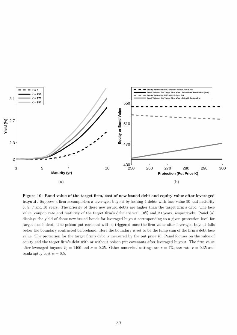
3 5 7 10
2
2.3
2.7
3.1
Maturity (yr)
Yie
ld (
%)
K = 0K = 250K = 270K = 290
250 260 270 280 290 300430
470
510
550
Protection (Put Price K)
Eq
uit
y o
r B
on
d V
alu
e
Equity Value after LBO without Poison Put (K=0)Bond Value of the Target Firm after LBO without Poison Put (K=0)Equity Value after LBO with Poison PutBond Value of the Target Firm after LBO with Poison Put
(a) (b)
Figure 10: Bond value of the target firm, cost of new issued debt and equity value after leveraged
buyout. Suppose a firm accomplishes a leveraged buyout by issuing 4 debts with face value 50 and maturity
3, 5, 7 and 10 years. The priority of these new issued debts are higher than the target firm’s debt. The face
value, coupon rate and maturity of the target firm’s debt are 250, 10% and 20 years, respectively. Panel (a)
displays the yield of those new issued bonds for leveraged buyout corresponding to a given protection level for
target firm’s debt. The poison put covenant will be triggered once the firm value after leveraged buyout falls
below the boundary contracted beforehand. Here the boundary is set to be the lump sum of the firm’s debt face
value. The protection for the target firm’s debt is measured by the put price K. Panel focuses on the value of
equity and the target firm’s debt with or without poison put covenants after leveraged buyout. The firm value
after leveraged buyout V0 = 1400 and σ = 0.25. Other numerical settings are r = 2%, tax rate τ = 0.35 and
bankruptcy cost α = 0.5.
30

5 Conclusion
If the market participants recognize the heterogeneity of corporate debt structure, then it is nature to
anticipate that market prices would account for this fact. Selectively simplifying this recognition prob-
ably leads to biased estimations. This article develops a theoretical framework to investigate the effects
of heterogeneous debt structure on the values of a firm’s claim holders from four observable facets
of corporate debt structure: the leverage ratio, maturity structure, priority structure and covenant
structure. Besides, we propose a novel numerical method to quantitatively analyze the behaviors of
the claim holders that are granted the rights to earlier redeem their bonds when the corporate debt
structure is complicated. Compared with extant credit risk models, the results generated by our
framework are more consistent with the real world phenomena documented already in empirical stud-
ies. First, our framework robustly generate upward-sloping credit spread curves for either investment-
or speculative-grade issuers as the observation by Helwege and Turner (1999) and Huang and Zhang
(2008), whereas numerous existing structural models may predict hump-shaped or downward-sloping
curves. Second, our framework not only predicts a positive correlation between a firm leverage ratio
and firm credit quality but also forecasts a negative relation between bond credit spreads and the
improvement in bond seniorities. If a bank debenture is replaced by a junior debenture issuance, the
credit spreads of the previously issued senior debenture may decrease because its relative priority in
the firm’s debt structure improves. Moreover, it predicts weak negative impacts of the presence of
short-term junior debenture on the prices of the existing long-term senior debenture when the issuing
firm is relatively healthy because there exists payment blockage covenants in the senior debenture, but
such impacts become significantly negative when the firm’s credit deteriorates because the blockage
period is limiting. Incorporating payment blockage into our framework makes our analyses regarding
the change of both maturity and priority structure in compliance with the empirical observation as
Linn and Stock (2005). Third, our framework predicts longer call delay because we jointly consider the
impacts of tax shield benefits and the wealth transfer effects on the firm’s optimal redemption policy.
We find that the wealth transfer effect may magnify the call delay phenomenon due to the presence of
tax shield benefits. Furthermore, we explains the conflicts between the theoretical predictions and the
empirical observations of the wealth transfer effects through the level of interest rate and the existence
of call protection covenants. Finally, our framework displays the salient impact of including poison
put covenants on the value of target bond holders and a potential bidder’s costs of debt financing. It
thus appears that accounting for the heterogeneity of corporate debt structure has a significant impact
on corporate bond valuation, and it helps to reconcile many of the predictions of extant structural
models with empirical observations.
31

References
Acharya, v. and J. Carpenter (2002). Corporate bond valuation and hedging with stochastic interest
rates and endogenous bankruptcy. Review of Financial Studies 15 (5), 1355–1383.
Altman, E. I. (1968). Financial ratios, discriminant analysis and the prediction of corporate
bankruptcy. Journal of Finance 23 (4), 589–609.
Asquith, P. (1995). Convertible bonds are not called late. Journal of Finance 50 (4), 1275–1289.
Attaoui, S. and P. Poncet (2013). Capital structure and debt priority. Financial Management .
Barnea, A., R. A. Haugen, and L. W. Senbet (1980). A rationale for debt maturity structure and call
provisions in the agency theoretic framework. Journal of Finance 35 (5), 1223–1234.
Billett, M. T., T.-H. D. King, and D. C. Mauer (2007). Growth opportunities and the choice of
leverage, debt maturity, and covenants. Journal of Finance 62 (2), 697–730.
Black, F. and J. Cox (1976). Valuing corporate securities: Some effects of bond indenture provisions.
Journal of Finance 31 (2), 351–367.
Black, F. and M. Scholes (1973). The pricing of options and corporate liabilities. Journal of Political
Economy 81 (3), 637.
Bodie, Z. and R. A. Taggart (1978). Future investment opportunities and the value of the call provision
on a bond. Journal of Finance 33 (4), 1187–1200.
Brennan, M. J. and E. S. Schwartz (1977). Savings bonds, retractable bonds and callable bonds.
Journal of Financial Economics 5 (1), 67–88.
Bris, A., I. Welch, and N. Zhu (2006). The costs of bankruptcy: Chapter 7 liquidation versus chapter
11 reorganization. Journal of Finance 61, 1253–1303.
Briys, E. and F. De Varenne (1997). Valuing risky fixed rate debt: An extension. Journal of Financial
and Quantitative Analysis 32 (2), 239–248.
Broadie, M. and O. Kaya (2007). A binomial lattice method for pricing corporate debt and modeling
chapter 11 proceedings. Journal of Financial and Quantitative Analysis 42, 1253–1303.
Colla, P., F. Ippolito, and K. Li (2013). Debt specialization. Journal of Finance.
Collin-Dufresne, P. and R. S. Goldstein (2001a). Do credit spreads reflect stationary leverage ratios?
Journal of Finance 56 (5), 1929–1957.
Collin-Dufresne, P., R. S. Goldstein, and J. S. Martin (2001b). The determinants of credit spread
changes. Journal of Finance 56 (6), 2177–2207.
Cook, D. O. and J. C. Easterwood (1994). Poison put bonds: An analysis of their economic role.
Journal of Finance 49 (5), 1905–1920.
Cox, J. C., S. A. Ross, and M. Rubinstein (1979). Option pricing: A simplified approach. Journal of
Financial Economics 7 (3), 229–263.
32

Crabbe, L. (1991). Event risk: An analysis of losses to bondholders and super poison put bond
covenants. Journal of Finance 46 (2), 689–706.
Crabbe, L. E. and J. Helwege (1994). Alternative tests of agency theories of callable corporate bonds.
Financial Management 23 (4), 3–20.
Cremers, K. M., V. B. Nair, and C. Wei (2007). Governance mechanisms and bond prices. Review of
Financial Studies 20 (5), 1359–1388.
Cummings, N., J. Thompson, and V. Paparo (January, 2009). Back to basics bnking. International
Financial Law Review .
Dai, T. and Y. Lyuu (2010). The bino-trinomial tree: A simple model for efficient and accurate option
pricing. Journal of Derivatives 17 (4), 7–24.
Dai, T.-S., C.-J. Wang, and Y.-D. Lyuu (2012). A multiphase, flexible, and accurate lattice for pricing
complex derivatives with multiple market variables. Journal of Futures Markets.
Davydenko, S. (2007). When do firms default? a study of the default boundary. American Finance
Association 2009 Annual Meeting .
Diamond, D. W. (1993). Seniority and maturity of debt contracts. Journal of Financial Eco-
nomics 33 (3), 341–368.
Duffie, D. (1996). Dynamic asset pricing theory. Princeton University Press.
Duffie, D. and K. J. Singleton (1999). Modeling term structures of defaultable bonds. Review of
Financial Studies 12 (4), 687–720.
Dunn, K. B. and C. S. Spatt (2005). The effect of refinancing costs and market imperfections on the
optimal call strategy and the pricing of debt contracts. Real Estate Economics 33 (4), 595–617.
Eom, Y. H., J. Helwege, and J.-z. Huang (2004). Structural models of corporate bond pricing: An
empirical analysis. Review of Financial Studies 17 (2), 499–544.
Fama, E. F. and M. H. Miller (1972). The Theory of Finance, Volume 3. Dryden Press Hinsdale, IL.
Fan, H. and S. M. Sundaresan (2000). Debt valuation, renegotiation, and optimal dividend policy.
Review of Financial Studies 13 (4), 1057–1099.
Figlewski, S. and B. Gao (1999). The adaptive mesh model: a new approach to efficient option pricing.
Journal of Financial Economics 53 (3), 313–351.
Fisher, L. (1984). Contingent claims analysis of corporate capital structures: An empirical investiga-
tion: Discussion. Journal of Finance 39 (3), 625–627.
Flannery, M. J., S. S. Nikolova, and O. Oztekin (2012). Leverage expectations and bond credit spreads.
Journal of Financial and Quantitative Analysis 47 (04), 689–714.
Geske, R. (1977). The valuation of corporate liabilities as compound options. Journal of Financial
and Quantitative Analysis 12 (04), 541–552.
Gryglewicz, S. (2011). A theory of corporate financial decisions with liquidity and solvency concerns.
Journal of Financial Economics 99 (2), 365–384.
33

Guedes, J. and T. Opler (1996). The determinants of the maturity of corporate debt issues. Journal
of Finance 51 (5), 1809–1833.
Hackbarth, D. and D. C. Mauer (2012). Optimal priority structure, capital structure, and investment.
Review of Financial Studies 25 (3), 747–796.
Harrison, J. M. and D. M. Kreps (1979). Martingales and arbitrage in multiperiod securities markets.
Journal of Economic Theory 20 (3), 381–408.
He, Z. and W. Xiong (2012). Rollover risk and credit risk. Journal of Finance 67 (2), 391–430.
Helwege, J. and C. M. Turner (1999). The slope of the credit yield curve for speculative-grade issuers.
Journal of Finance 54 (5), 1869–1884.
Huang, J.-z. and M. Huang (2012). How much of the corporate-treasury yield spread is due to credit
risk? Review of Asset Pricing Studies 2 (2), 153–202.
Huang, J.-Z. and X. Zhang (2008). The slope of credit spread curves. Journal of Fixed Income 18 (1),
56–71.
Hull, J. (2012). Options, Futures, and Other Derivatives, 8/e. Pearson Education India.
Ingersoll, J. E. (1977a). A contingent-claims valuation of convertible securities. Journal of Financial
Economics 4 (3), 289–321.
Ingersoll, J. E. (1977b). An examination of corporate call policies on convertible securities. Journal
of Finance 32 (2), 463–478.
Ingersoll, J. E. (1987). Theory of financial decision making, Volume 3. Rowman & Littlefield.
Jarrow, R. A., D. Lando, and S. M. Turnbull (1997). A markov model for the term structure of credit
risk spreads. Review of Financial Studies 10 (2), 481–523.
Jarrow, R. A. and S. M. Turnbull (1995). Pricing derivatives on financial securities subject to credit
risk. Journal of Finance 50 (1), 53–85.
Jensen, M. C. and W. H. Meckling (1976). Theory of the firm: Managerial behavior, agency costs and
ownership structure. Journal of Financial Economics 3 (4), 305–360.
Jones, E. P., S. P. Mason, and E. Rosenfeld (1984). Contingent claims analysis of corporate capital
structures: An empirical investigation. Journal of Finance 39 (3), 611–625.
Ju, N. and H. Ou-Yang (2006). Capital structure, debt maturity, and stochastic interest rates*.
Journal of Business 79 (5), 2469–2502.
Jung, M., R. B. Ellis, and M. Epplin (2012). Do call provisions reduce agency costs of debt irrespective
of maturity and seniority? Mustang Journal of Accounting and Finance 2, 36.
Kim, I., K. Ramaswamy, and S. Sundaresan (1993). Does default risk in coupons affect the valuation
of corporate bonds?: A contingent claims model. Financial Management 22 (3), 117–131.
King, T.-H. D. (2002). An empirical examination of call option values implicit in us corporate bonds.
Journal of Financial and Quantitative Analysis 37 (04), 693–721.
34
King, T.-H. D. and D. C. Mauer (2000). Corporate call policy for nonconvertible bonds*. Journal of
Business 73 (3), 403–444.
Kisgen, D. J. (2006). Credit ratings and capital structure. Journal of Finance 61 (3), 1035–1072.
Kish, R. J. and M. Livingston (1992). Determinants of the call option on corporate bonds. Journal
of Banking and Finance 16 (4), 687–703.
Lando, D. (2004). Credit risk modeling: theory and applications. Princeton University Press.
Leland, H. E. (1994). Corporate debt value, bond covenants, and optimal capital structure. Journal
of Finance 49 (4), 1213–1252.
Leland, H. E. and K. B. Toft (1996). Optimal capital structure, endogenous bankruptcy, and the term
structure of credit spreads. Journal of Finance 51 (3), 987–1019.
Linn, S. C. and D. R. Stock (2005). The impact of junior debt issuance on senior unsecured debts risk
premiums. Journal of Banking and Finance 29 (6), 1585–1609.
Longstaff, F. A. and E. S. Schwartz (1995). A simple approach to valuing risky fixed and floating rate
debt. Journal of Finance 50 (3), 789–819.
Longstaff, F. A. and B. A. Tuckman (1994). Calling nonconvertible debt and the problem of related
wealth transfer effects. Financial Management 23 (4), 21–27.
Madan, D. B. and H. Unal (1998). Pricing the risks of default. Review of Derivatives Research 2 (2-3),
121–160.
Mauer, D. C. (1993). Optimal bond call policies under transactions costs. Journal of Financial
Research 16 (1), 23–37.
Merton, R. C. (1974). On the pricing of corporate debt: The risk structure of interest rates*. Journal
of Finance 29 (2), 449–470.
Modigliani, F. and M. H. Miller (1958). The cost of capital, corporation finance and the theory of
investment. American Economic Review 48 (3), 261–297.
Myers, S. C. (1977). Determinants of corporate borrowing. Journal of Financial Economics 5 (2),
147–175.
Park, C. (2000). Monitoring and structure of debt contracts. Journal of Finance 55 (5), 2157–2195.
Rauh, J. D. and A. Sufi (2010). Capital structure and debt structure. Review of Financial Stud-
ies 23 (12), 4242–4280.
Sarkar, S. (2004). Yield spreads, agency costs and the corporate bond call feature. European Journal
of Finance 10 (4), 308–327.
Sinkey, J. (2002). Commercial Bank Financial Management in the Financial Services Industry. New
York: Macmillan.
Smith, C. W. and J. B. Warner (1979). On financial contracting: An analysis of bond covenants.
Journal of Financial Economics 7 (2), 117–161.
35