Embed Size (px)
Citation preview
Evaluating Alternate Classification Algorithms in First Party Retail Banking Fraud Author: Kevin Barrett
Co-Authors: Xin Huang, Will Boulter
27-30th AUGUST 2013
2
Submission
Evaluating alternate classification algorithms in first party retail banking fraud
This presentation will be a discussion of alternative approaches for first-party fraud classification modelling.
Currently, the primary classification approach for the first-party fraud modelling problems within Lloyds Banking Group is logistic
regression. Since a wide range of studies both in academia and industry suggest several state-of-the-art classification algorithms
can outperform logistic regression, we have investigated promising alternative algorithms to understand how they can improve
classification performance.
We have assessed these algorithms on two different fraud problems; first party application fraud and post-application mule fraud.
The nature of the fraud problems assessed, specifically the limited, but highly costly, number of bad customers and the operational
constraints in working target accounts leads us to use bespoke criteria in evaluating the performance of different classification
algorithms.
Various methods, including neural networks, support vector machines and random forests have been assessed as potential
alternate approaches. These have been assessed on classification performance using general statistical benchmarks as well as
our bespoke criteria relevant to these fraud problems. Additionally, these approaches have been evaluated on computational
efficiency, ease of tuning, complexity and ease of management within a banking environment.
The presentation will cover a brief introduction to the problem types and algorithms, followed by a discussion of findings and
recommendations.
3
Motivation Identify the best classification algorithm to classify 1st Party Fraud
Evaluating alternate classification algorithms in first party retail banking fraud
There are many classification algorithms currently in use across both industry and academia.
For many reasons including simplicity, robustness and familiarity, the banking industry tend to assess binary classification
problems (such as default/non-default, response,/non-response, etc.) using logistic regression.
The requirements of a classification algorithm to identify fraud are different to those of a typical credit risk model for the
following reasons:
Fraud events are extremely rare so the algorithm needs to be able to deal with a target that typically constitutes <1% of
the modelling population.
Model interpretability is lower on the priority list than outright performance as the customer is typically unaware that their
transaction/application is being scored
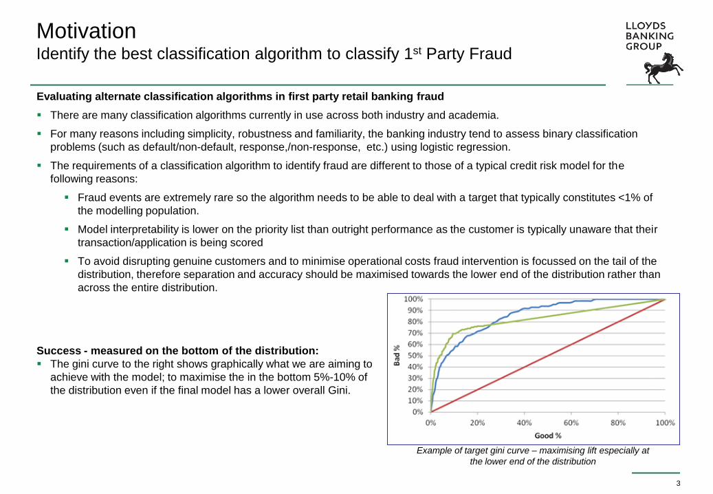
To avoid disrupting genuine customers and to minimise operational costs fraud intervention is focussed on the tail of the
distribution, therefore separation and accuracy should be maximised towards the lower end of the distribution rather than
across the entire distribution.
Success - measured on the bottom of the distribution:
The gini curve to the right shows graphically what we are aiming to
achieve with the model; to maximise the in the bottom 5%-10% of
the distribution even if the final model has a lower overall Gini.
Example of target gini curve – maximising lift especially at
the lower end of the distribution
4
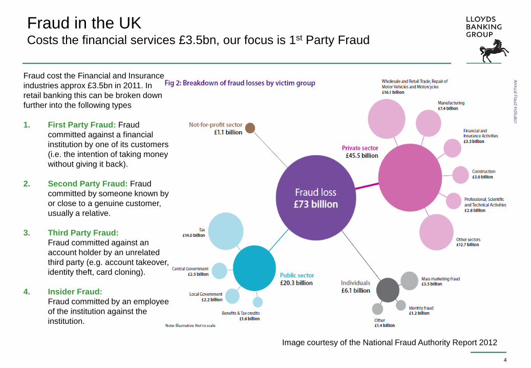
Fraud in the UK Costs the financial services £3.5bn, our focus is 1st Party Fraud
Fraud cost the Financial and Insurance
industries approx £3.5bn in 2011. In
retail banking this can be broken down
further into the following types
1. First Party Fraud: Fraud
committed against a financial
institution by one of its customers
(i.e. the intention of taking money
without giving it back).
2. Second Party Fraud: Fraud
committed by someone known by
or close to a genuine customer,
usually a relative.
3. Third Party Fraud:
Fraud committed against an
account holder by an unrelated
third party (e.g. account takeover,
identity theft, card cloning).
4. Insider Fraud:
Fraud committed by an employee
of the institution against the
institution.
Image courtesy of the National Fraud Authority Report 2012
5
Approach to Identifying Alternative Algorithms We have worked closely with two leading universities to explore the options
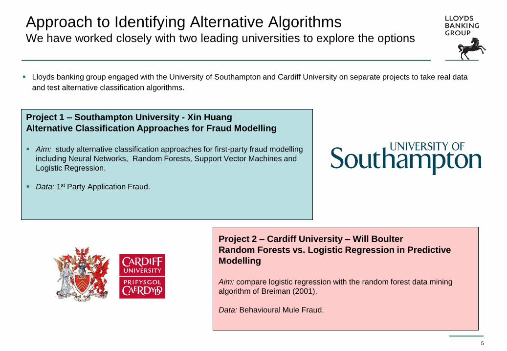
Lloyds banking group engaged with the University of Southampton and Cardiff University on separate projects to take real data
and test alternative classification algorithms.
Project 1 – Southampton University - Xin Huang
Alternative Classification Approaches for Fraud Modelling
Aim: study alternative classification approaches for first-party fraud modelling
including Neural Networks, Random Forests, Support Vector Machines and
Logistic Regression.
Data: 1st Party Application Fraud.
Project 2 – Cardiff University – Will Boulter
Random Forests vs. Logistic Regression in Predictive
Modelling
Aim: compare logistic regression with the random forest data mining
algorithm of Breiman (2001).
Data: Behavioural Mule Fraud.

Result:
• The neural network and random forest achieve the
highest performance compared to the others, in
terms of both gini coefficient and the level of
cumulative bad at the 5% cut-off point.
6
Project 1 – Southampton University - Xin Huang On application fraud data, Neural Networks and Random forests prove to be
the most effective classification algorithms
Project: Alternative Classification Approaches for Fraud Modelling
Study alternative classification approaches for first-party application fraud modelling including :
Logistic Regression
Neural Networks
Random Forests
Support Vector Machines
Sample:- Current Account applications over an extended
period (> 200k observations)
Outcome Window: 12 months
Fraud Flag:-
1. Charged-off as 1st Party Fraud with loss
2. Identified as an account used for Mule fraud
3. Account intervention by fraud operations
Model Predictors:
Customer information both from the application form
and the bureau records. Reduced to 112 variables
after eliminating weak predictors.
Validation:
The data set is split into three parts: training,
validation and test. All results come from the testing
set.
Technique Gini
Coefficient
Cumulative Bad
at 5%
Logistic Regression (WoE)
61.8% 29%
Neural Networks 65.6% 36%
SVM 64.5% 31%
Random Forest 65.2% 36%
Logistic Regression2 (raw data) 64% 33%
Modelling Dataset:
7
Project 1 – Southampton University - Xin Huang The advantage over logistic regression is modest
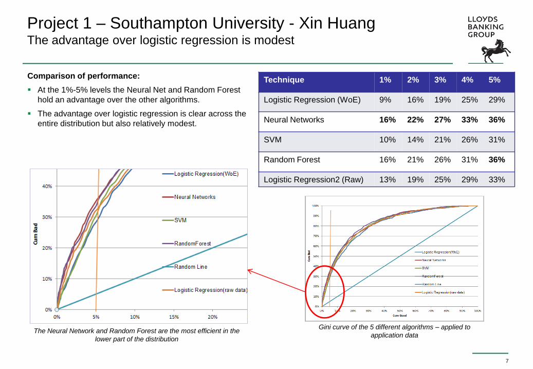
Comparison of performance:
At the 1%-5% levels the Neural Net and Random Forest
hold an advantage over the other algorithms.
The advantage over logistic regression is clear across the
entire distribution but also relatively modest.
Technique 1% 2% 3% 4% 5%
Logistic Regression (WoE) 9% 16% 19% 25% 29%
Neural Networks 16% 22% 27% 33% 36%
SVM 10% 14% 21% 26% 31%
Random Forest 16% 21% 26% 31% 36%
Logistic Regression2 (Raw) 13% 19% 25% 29% 33%
Gini curve of the 5 different algorithms – applied to
application data The Neural Network and Random Forest are the most efficient in the
lower part of the distribution
8
Project 1 – Southampton University - Xin Huang Once additional factors are considered, Random Forests offer the most
promise. There may also be further opportunity in combining approaches
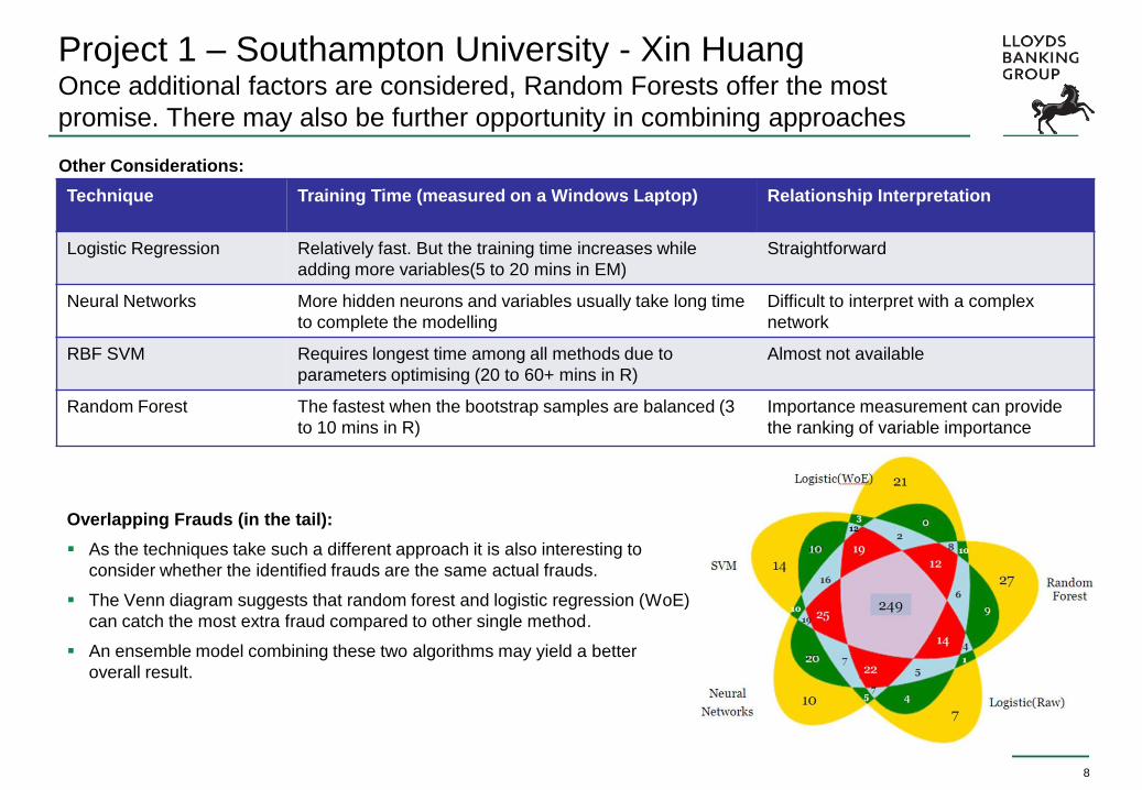
Overlapping Frauds (in the tail):
As the techniques take such a different approach it is also interesting to
consider whether the identified frauds are the same actual frauds.
The Venn diagram suggests that random forest and logistic regression (WoE)
can catch the most extra fraud compared to other single method.
An ensemble model combining these two algorithms may yield a better
overall result.
Technique Training Time (measured on a Windows Laptop) Relationship Interpretation
Logistic Regression
Relatively fast. But the training time increases while
adding more variables(5 to 20 mins in EM)
Straightforward
Neural Networks
More hidden neurons and variables usually take long time
to complete the modelling
Difficult to interpret with a complex
network
RBF SVM Requires longest time among all methods due to
parameters optimising (20 to 60+ mins in R)
Almost not available
Random Forest
The fastest when the bootstrap samples are balanced (3
to 10 mins in R)
Importance measurement can provide
the ranking of variable importance
Other Considerations:
9
Project 1 – Southampton University - Xin Huang Conclusion: Random forests are recommended for further study
All of these three alternative methods are worthy of further investigation given their ability to explain the non-linear patterns of the
data set; e.g. neural networks and random forests can perform at least as well as logistic regression classification.
Random forests are highly recommended for further study since they require less training time, give relatively high performance
and provide a useful variable importance measurement output.
Various fraud modelling approaches should be viewed as complementary rather than competitors. They can be used in
conjunction to detect different fraudsters.
To get a performance boost from neural networks, support vector machines or random forests, more variables are needed for
training. Therefore, from a business perspective, their benefits must be balanced against the cost of processing more variables
and also their potential instability.
Random Forests vs. Logistic Regression in Predictive Modelling
Project: Compare logistic regression with the relatively new random forest data mining algorithm of Breiman (2001), which
has become popular because of its high accuracy and ability to handle large datasets.
Approach: Build a behavioural model on current accounts that have been open for less than a year and identify which
accounts will go on to commit mule fraud within a week. To replicate current practice and to deal with the large volume of
data, the approach will be supplemented with an exclusion model.
The techniques being compared are:
1. Simplistic Logistic Regression
2. Dual stage Logistic Regression
3. Dual stage Random Forests
10
Project 2 – Cardiff University – Will Boulter Compare simple & dual stage Logistic Regression with Random Forests on
behavioural dataset to identify Mule Fraud
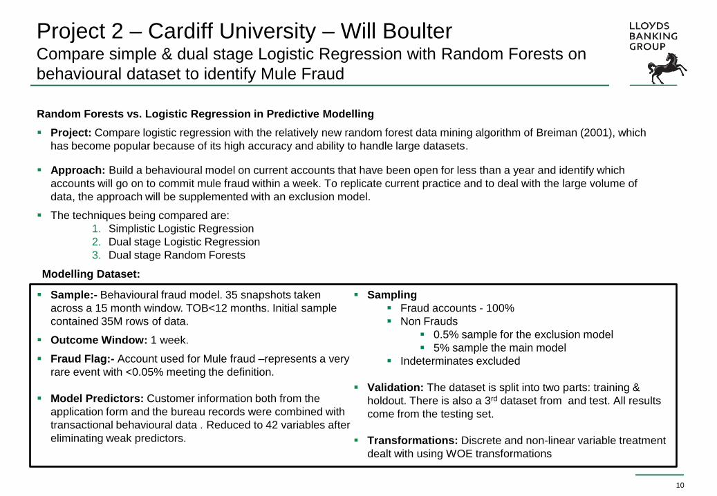
Sample:- Behavioural fraud model. 35 snapshots taken
across a 15 month window. TOB<12 months. Initial sample
contained 35M rows of data.
Outcome Window: 1 week.
Fraud Flag:- Account used for Mule fraud –represents a very
rare event with <0.05% meeting the definition.
Model Predictors: Customer information both from the
application form and the bureau records were combined with
transactional behavioural data . Reduced to 42 variables after
eliminating weak predictors.
Sampling
Fraud accounts - 100%
Non Frauds
0.5% sample for the exclusion model
5% sample the main model
Indeterminates excluded
Validation: The dataset is split into two parts: training &
holdout. There is also a 3rd dataset from and test. All results
come from the testing set.
Transformations: Discrete and non-linear variable treatment
dealt with using WOE transformations
Modelling Dataset:
Exclusion model Gini is stable across validation samples
11
Project 2 – Cardiff University – Will Boulter Exclusion model developed as a simple logistic regression model with a gini
of 71.3%
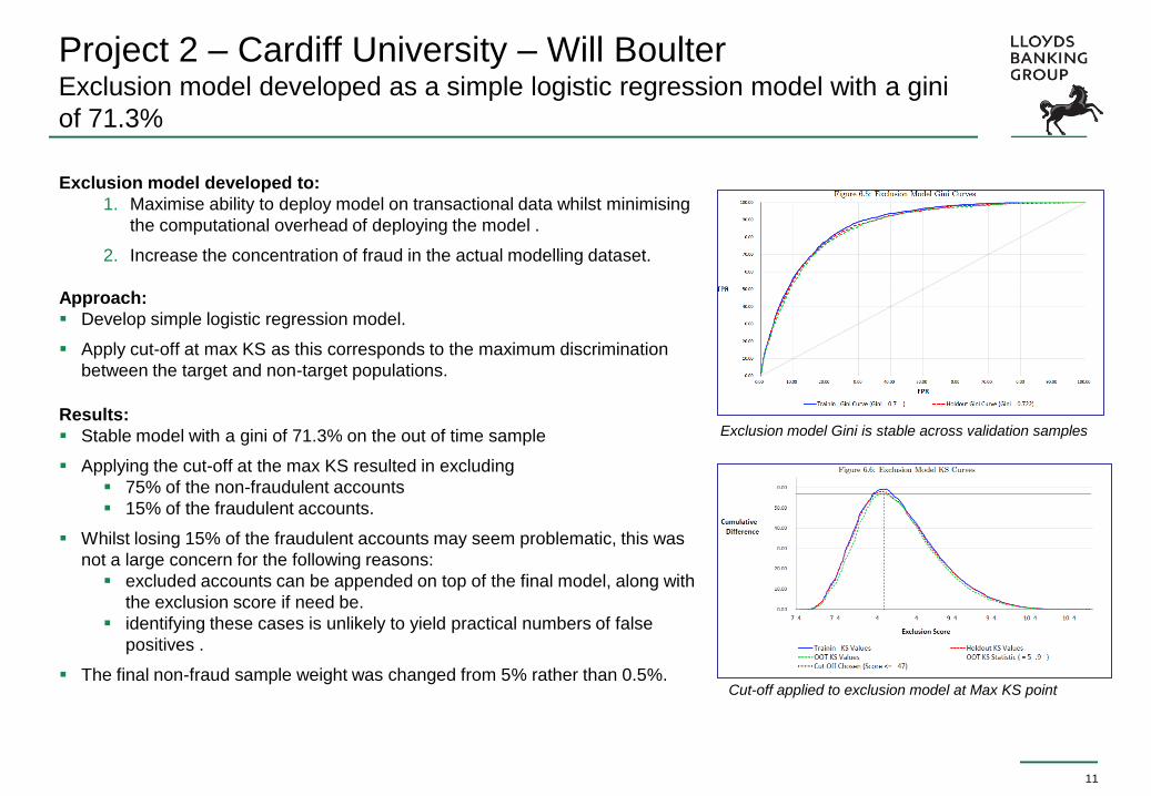
Exclusion model developed to:
1. Maximise ability to deploy model on transactional data whilst minimising
the computational overhead of deploying the model .
2. Increase the concentration of fraud in the actual modelling dataset.
Approach:
Develop simple logistic regression model.
Apply cut-off at max KS as this corresponds to the maximum discrimination
between the target and non-target populations.
Results:
Stable model with a gini of 71.3% on the out of time sample
Applying the cut-off at the max KS resulted in excluding
75% of the non-fraudulent accounts
15% of the fraudulent accounts.
Whilst losing 15% of the fraudulent accounts may seem problematic, this was
not a large concern for the following reasons:
excluded accounts can be appended on top of the final model, along with
the exclusion score if need be.
identifying these cases is unlikely to yield practical numbers of false
positives .
The final non-fraud sample weight was changed from 5% rather than 0.5%.
Cut-off applied to exclusion model at Max KS point
12
Project 2 – Cardiff University – Will Boulter Dual Stage Logistic Model delivers a gini of 75.2% and significant lift at the
lower end of the distribution
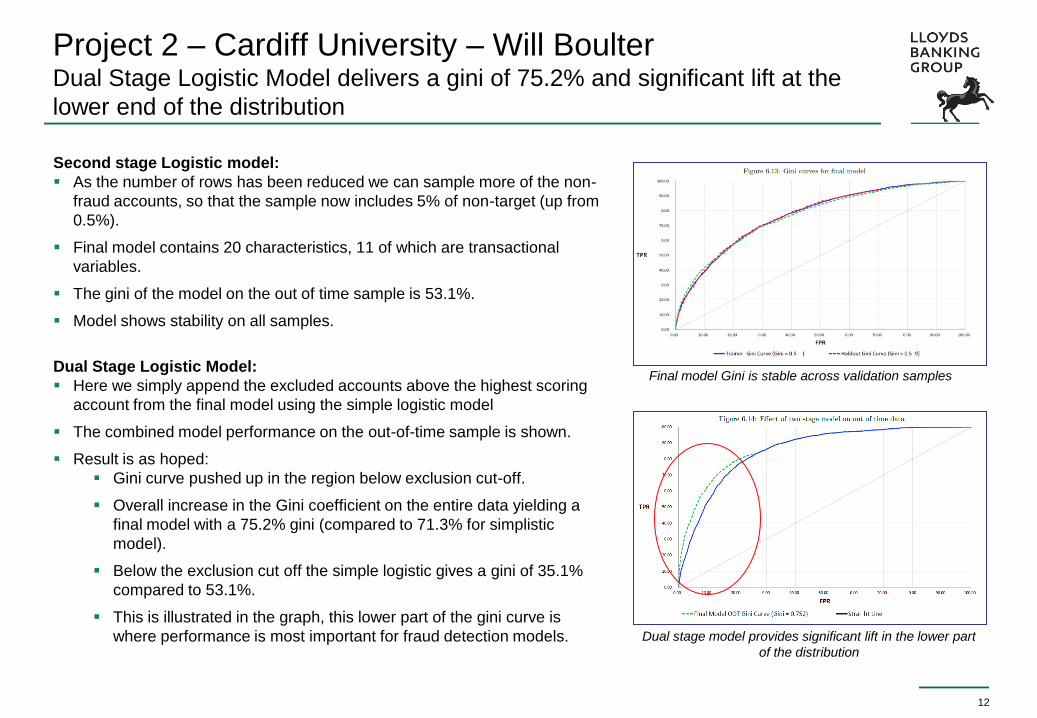
Second stage Logistic model:
As the number of rows has been reduced we can sample more of the non-
fraud accounts, so that the sample now includes 5% of non-target (up from
0.5%).
Final model contains 20 characteristics, 11 of which are transactional
variables.
The gini of the model on the out of time sample is 53.1%.
Model shows stability on all samples.
Dual Stage Logistic Model:
Here we simply append the excluded accounts above the highest scoring
account from the final model using the simple logistic model
The combined model performance on the out-of-time sample is shown.
Result is as hoped:
Gini curve pushed up in the region below exclusion cut-off.
Overall increase in the Gini coefficient on the entire data yielding a
final model with a 75.2% gini (compared to 71.3% for simplistic
model).
Below the exclusion cut off the simple logistic gives a gini of 35.1%
compared to 53.1%.
This is illustrated in the graph, this lower part of the gini curve is
where performance is most important for fraud detection models.
Final model Gini is stable across validation samples
Dual stage model provides significant lift in the lower part
of the distribution
13
Project 2 – Cardiff University – Will Boulter Random Forest has a higher gini but Logistic Regression works better at the
bottom of the distribution
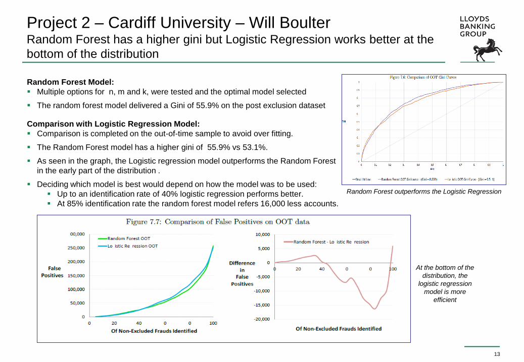
Random Forest Model:
Multiple options for n, m and k, were tested and the optimal model selected
The random forest model delivered a Gini of 55.9% on the post exclusion dataset
Comparison with Logistic Regression Model:
Comparison is completed on the out-of-time sample to avoid over fitting.
The Random Forest model has a higher gini of 55.9% vs 53.1%.
As seen in the graph, the Logistic regression model outperforms the Random Forest
in the early part of the distribution .
Deciding which model is best would depend on how the model was to be used:
Up to an identification rate of 40% logistic regression performs better.
At 85% identification rate the random forest model refers 16,000 less accounts.
Random Forest outperforms the Logistic Regression
At the bottom of the
distribution, the
logistic regression
model is more
efficient
14
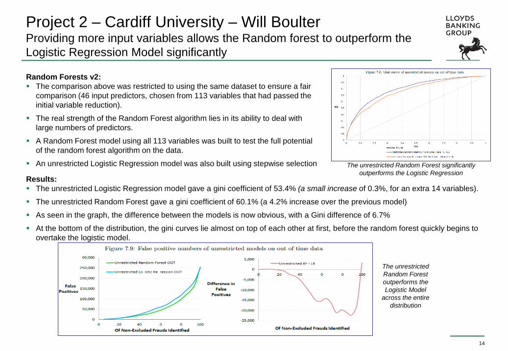
Project 2 – Cardiff University – Will Boulter Providing more input variables allows the Random forest to outperform the
Logistic Regression Model significantly
Random Forests v2:
The comparison above was restricted to using the same dataset to ensure a fair
comparison (46 input predictors, chosen from 113 variables that had passed the
initial variable reduction).
The real strength of the Random Forest algorithm lies in its ability to deal with
large numbers of predictors.
A Random Forest model using all 113 variables was built to test the full potential
of the random forest algorithm on the data.
An unrestricted Logistic Regression model was also built using stepwise selection
Results:
The unrestricted Logistic Regression model gave a gini coefficient of 53.4% (a small increase of 0.3%, for an extra 14 variables).
The unrestricted Random Forest gave a gini coefficient of 60.1% (a 4.2% increase over the previous model)
As seen in the graph, the difference between the models is now obvious, with a Gini difference of 6.7%
At the bottom of the distribution, the gini curves lie almost on top of each other at first, before the random forest quickly begins to
overtake the logistic model.
The unrestricted Random Forest significantly
outperforms the Logistic Regression
The unrestricted
Random Forest
outperforms the
Logistic Model
across the entire
distribution
15
Project 2 – Cardiff University – Will Boulter Random Forests consistently outperform Logistic Regression especially
when trained on datasets with a large number of predictors
Conclusion:
In terms of the gini coefficient, the Random Forest algorithm consistently outperforms logistic regression .
The performance gap between the Random Forest and Logistic Regression models seems to be dependent on the number of
variables available.
For fraud, our aim is to maximise the separation in the lower part of the distribution. Here we saw the logistic regression
outperform random forests in a very small percentage of the overall population, but one which corresponded to around 34% of
the accounts used for mule fraud (until we made more variables available).
There are some additional promising avenues for future research after this project. One technique for consideration is referred
to as “model blending” and involves combining many different types of models to achieve a better prediction.
16
Overall Conclusion Logistic Regression is one of the best algorithms available for classifying
fraud. However, Random Forests can consistently outperform regression.
Conclusion:
Of the various approaches reviewed, Random Forests has emerged as the most likely algorithm to replace Logistic
Regression for classifying fraud data as it can provide:
Better rank ordering across the whole score distribution
The model retains some interpretability through the importance statistic
The relatively simple computational demands allow fast processing of large dataset
Next Steps:
The projects described here have been built using the limited processing power of a single laptop computer however the
results have still been compelling. We hope to build and deploy a Random forest over the next 12-18 months using a much
more powerful server which we expect to yield even more impressive results.
Beyond Random Forests, both of the projects have suggested that further opportunities may be available by combining
multiple approaches together to fully maximise efficiency.

Questions?
For further enquiries on this project or to discuss recruitment opportunities please contact me directly:
17

18
Appendix: Introduction to the Random Forest Algorithm Random Forests introduced by Breiman in 2001 is based on decision tree’s
using bootstrapping and aggregating (‘bagging’)
Random Forests:
Uses CART (Classification and Regression Trees) – developed by Breiman in 1984
Breiman introduced random forests in 2001 which combines 2 concepts:
1. Consider a random subset of variables at each decision point
2. Aggregate the results of several models, each built on a different bootstrap
sample (random sampling with replacement). Breiman combined the words
‘bootstrap’ and ‘aggregating’ to coin the phrase ‘bagging’
Algorithm Overview:
1. Take a data set of size N, with M prospective predictors and a target variable Y (this will be binary).
2. Choose the parameters (these should be adjusted for optimal performance):
• n - the number of trees to build,
• m - the number of variables to consider at each split. By default this is set to ⌊√M⌋, • k - the percentage of the original data to be used as training data. By default k ≈ 63% of the original.
3. Take a sample of k% of the observations from the original data. The left over data is referred to as out of bag or OOB
data.
4. Build a full decision tree on the training data, using the CART algorithm with one alteration: At each node, only consider a
random subset of m of the M possible predictors with which to split.
5. Estimate the generalisation error of the forest so far using the OOB data.
6. Take a new sample of the original data (with replacement), and repeat steps 4 and 5.
7. Repeat step 6 until n trees have been built.
8. When this iterative process ends, the forest is complete. To make a prediction about a new observation we send it through
each decision tree until it reaches a leaf. If this leaf contained a majority of class 1 during the training stage, then the tree
votes for class 1 - otherwise it votes for class 2 (in the unlikely case of a tie, the vote is selected randomly). The votes
from each tree in the forest are added up, and used to make a prediction about the class of the unlabelled observation.