EVA Robotic Assistant Project: Platform Attitude Prediction

Kevin Nickels ninity University

ER4 August 10,2000

b n e t h Baker ERLuRobotic Systems Technology Branch

Automation, Robotics, & Simulation Division Engin&g Directorate

Kevin Nickels

https://ntrs.nasa.gov/search.jsp?R=20030064068 2018-06-12T14:08:13+00:00Z

EVA Robotic Assistant Project:

Platform Attitude Prediction

Final Report

NASNASEE Summer Faculty Fellowship Program - 2000

Johnson Space Center

Prepared By:

Academic Rank:

University & Department:

NASNJSC

Directorate:

Division:

Branch:

JSC Colleague:

Date Submitted:

Contract Number:

Kevin M. Nickels, Ph. D.

Assistant Professor

Trinity University

Department of Engineering Science

San Antonio TX 782 12

Engineering

Automation, Robotics & Simulation Division

Robotic Systems Technology Branch

Kenneth Baker

August 10,2000

NAG 9-867

11-1

ABSTRACT

The Robotic Systems Technology Branch is currently working on the development of an EVA Robotic Assistant under the sponsorship of the Surface Systems Thrust of the NASA Cross Enter- prise Technology Development Program (CETDP). This will be a mobile robot that can follow a field geologist during planetary surface exploration, carry his tools and the samples that he collects, and provide video coverage of his activity.

Prior experiments have shown that for such a robot to be useful it must be able to follow the geologist at walking speed over any terrain of interest. Geologically interesting terrain tends to be rough rather than smooth. The commercial mobile robot that was recently purchased as an initial testbed for the EVA Robotic Assistant Project, an ATRV Jr., is capable of faster than wallring speed outside but it has no suspension. Its wheels with inflated rubber tires are attached to axles that are connected directly to the robot body. Any angular motion of the robot produced by driving over rough terrain will directly affect the pointing of the on-board stereo cameras. The resulting image motion is expected to make tracking of the geologist more difficult. This will either require the tracker to search a larger part of the image to find the target from frame to frame or to search mechanically in pan and tilt whenever the image motion is large enough to put the target outside of the image in the next frame.

This project consists of the design and implementation of a Kalman filter that combines the output of the angular rate sensors and linear accelerometers on the robot to estimate the motion of the robot base. The motion of the stereo camera pair mounted on the robot that results from this motion as the robot drives over rough terrain is then straightforward to compute.

The estimates may then be used, for example, to command the robot’s on-board pan-tilt unit to compensate for the camera motion induced by the base movement. This has been accomplished in two ways: first, a standalone head stabilizer has been implemented and second, the estimates have been used to influence the search algorithm of the stereo tracking algorithm. Studies of the image motion of a tracked object indicate that the image motion of objects is suppressed while the robot is crossing rough terrain.

This work expands the range of speed and surface roughness over which the robot should be able to track and follow a field geologist and accept arm gesture commands from the geologist.

11-2

INTRODUCTION

The focus of this work is to develop a high-fidelity estimate of the angular orientation and angular velocity of the robot base. Sensors that are utilized to arrive at this estimate include three mutually orthogonal gyrometers, three mutually orthogonal linear accelerometers, and a magnetic compass.

The estimates may then be used, for example, to command the robot’s on-board pan-tilt unit to compensate for the camera motion induced by the base movement. This has been accomplished in two ways: first, a standalone head stabilizer has been implemented and second, the estimates have been used to influence the search algorithm of the stereo tracking algorithm.

Rover Hardware

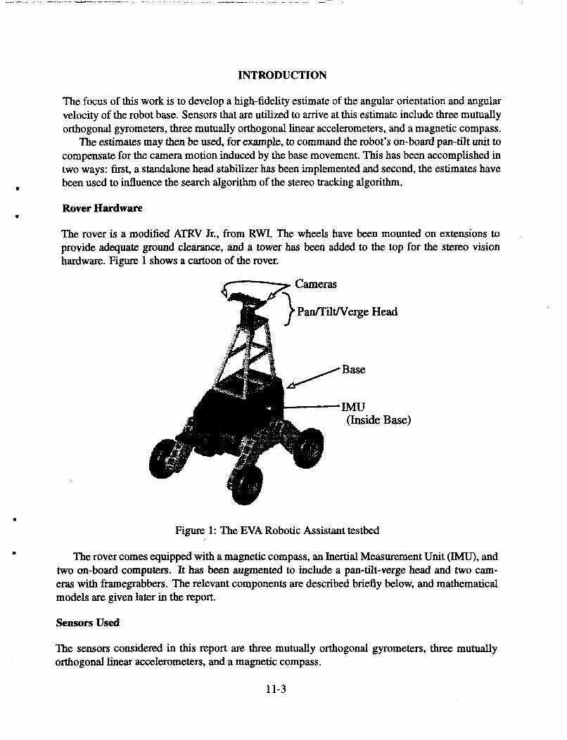
The rover is a modified ATRV Jr., from RWI. The wheels have been mounted on extensions to provide adequate ground clearance, and a tower has been added to the top for the stereo vision hardware. Figure 1 shows a cartoon of the rover.

IMU (Inside Base)

0

Figure 1: The EVA Robotic Assistant testbed

e The rover comes equipped with a magnetic compass, an Inertial Measurement Unit (IMU), and two on-board computers. It has been augmented to include a pan-tilt-verge head and two cam- eras with framegrabbers. The relevant components are described briefly below, and mathematical models are given later in the report.

sensors used

The sensors considered in this report are three mutually orthogonal gyrometers, three mutually orthogonal linear accelerometers, and a magnetic compass.

11-3

A gyrometer measures angular velocity about a single axis. These measurements are corrupted by gyro biases [3]. These biases are commonly estimated for purposes of compensation (see below for mathematical sensor models used.) After compensation, the angular rates recovered can be integrated to arrive at an estimate of the rotation of a body relative to some fixed initial orientation.

A linear accelerometer measures acceleration along a single axis. The accelerations can be integrated to arrive at linear velocities, and integrated again to arrive at position relative to some initial position. In this work, the accelerometers were not used in this fashion, but were used to measure the direction of the gravitational vector while the rover was at rest. See [SI for more discussion on inertial data.

The linear accelerometers and gyros used in this project were packaged in a single Inertial Measurement Unit (IMU), the DMU-6X from Crossbow. A magnetic compass yields a bearing with respect to magnetic north. The magnetic compass used in this project was the TCM2 from Precision Navigation.

Actuators Used

The stereo pan-tilt-verge (PTV) heads considered in this report are the Zebra Vergence from Pyxis Corp (formerly Helpmate, formerly TRC) and the Biclops from Metrica. Each of these heads accepts movement commands via a serial port from an external computer. Each head supports two cameras, which are used for image acquisition.

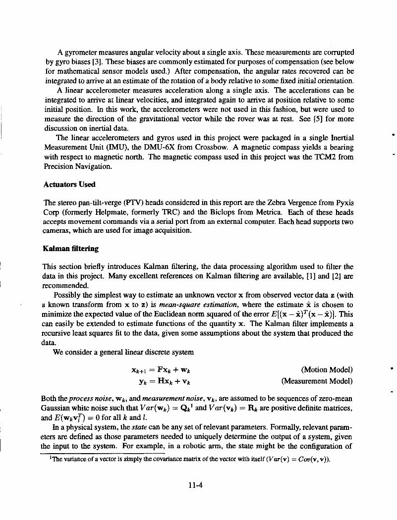
Kalman filtering

This section briefly introduces Kalman filtering, the data processing algorithm used to filter the data in this project. Many excellent references on Kalman filtering are available, [I] and [2] are recommended.

Possibly the simplest way to estimate an unknown vector x from observed vector data z (with a known transform from x to z) is mean-square estimation, where the estimate 12 is chosen to minimize the expected value of the Euclidean nom squared of the error E[(x - k)'(x - 12)) This can easily be extended to estimate functions of the quantity x. The Kalman filter implements a recursive least squares fit to the data, given some assumptions about the system that produced the data.

We consider a general linear discrete system

(Motion Model) (Measurement Model)

Both theprocess noise, wt, and measurement noise, vk , are assumed to be sequences of zero-mean Gaussian white noise such that Var(wk) = Q k l and Var(vk) = R k are positive definite matrices, and E(wkv7) = 0 for all k and 1.

In a physical system, the state can be any set of relevant parameters. Formally, relevant param- eters are dehed as those parameters needed to uniquely determine the output of a system, given the input to the system. For example, in a robotic arm, the state might be the configuration of

'The variance of a vector is simply the covariance matrix of the vector with itself <Var(v) = COV(V, v)).

11-4

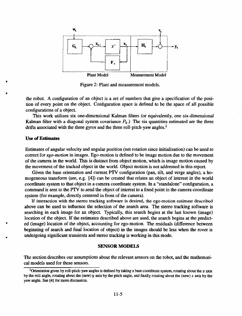
Figure 2: Plant and measurement models.

the robot. A configuration of an object is a set of numbers that give a specification of the posi- tion of every point on the object. Configuration space is defined to be the space of all possible configurations of a object.

This work utilizes six onedimensional Kalman filters (or equivalently, one six-dimensional Kalman filter with a diagonal system covariance Pk.) The six quantities estimated are the three drifts associated with the three gyros and the three roll-pitch-yaw angles.2

Use of Estimates

Estimates of angular velocity and angular position (net rotation since initialization) can be used to correct for ego-motion in images. Ego-motion is defined to be image motion due to the movement of the camera in the world. This is distinct from object motion, which is image motion caused by the movement of the tracked object in the world. Object motion is not addressed in this report.

Given the base orientation and current PTV configuration (pan, tilt, and verge angles), a ho- mogeneous transform (see, e.g. [4]) can be created that relates an object of interest in the world coordinate system to that object in a camera coordinate system. In a “standalone” configuration, a command is sent to the PTV to send the object of interest to a fixed point in the camera coordinate system (for example, directly centered in front of the camera).

If’ interaction with the stereo tracking software is desired, the ego-motion estimate described above can be used to influence the selection of the search area. The stereo tracking software is searching in each image for an object. Typically, this search begins at the last known (image) location of the object. If the estimates described above are used, the search begins at the predict-

beginning of search and final location of object) in the images should be less when the rover is b ed (image) location of the object, accounting for ego-motion. The residuals (difference between

8 undergoing significant transients and stereo tracking is working in this mode.

SENSOR MODELS

The section describes our assumptions about the relevant sensors on the robot, and the mathemati- cal models used for these sensors.

‘Orientation given by roll-pitch-yaw angles is defined by taking a base coordinate system, rotating about the z axis by the roll angle, rotating about the (new) y axis by the pitch angle, and finally rotating about the (new) z axis by the yaw angle. See [4] for more discussion.

11-5

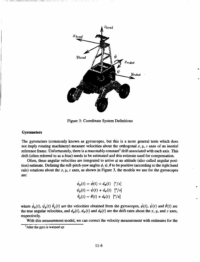
Figure 3: Coordinate System Definitions

Gyrometers

The gyrometers (commonly known as gyroscopes, but this is a more general term which does not imply rotating machinexy) measure velocities about the orthogonal x, y, x axes of an inertial reference frame. Unfortunately, there is a reasonably constant3 drift associated with each axis. This drift (often referred to as a bias) needs to be estimated and this estimate used for compensation.

Often, these angular velocities are integrated to arrive at an attitude (also called angular posi- tion) estimate. Defining the roll-pitch-yaw angles 4, $, 8 to be positive (according to the right hand rule) rotations about the z, g, z axes, as shown in Figure 3, the models we use for the gyroscopes are:

where #g(t), $,(t) t$(t) are the velocities obtained from the gyroscopes, &t), $(t) and b(t) are the true angular velocities, and $4(t) , d$(t) and &(t) are the drift rates about the x, y, and z axes, respectively.

With this measurement model, we can correct the velocity measurement with estimates for the 3 ~ t e r the gyro is warmed up

11-6

drift rates as follows

assuming the drift rates are known.

Accelerometers

The three on-board accelerometers measure accelerations along orthogonal x, y, z axes of their local reference frame. These accelerations can be integrated to arrive at estimates for velocity. The velocity estimates may then be integrated to arrive at estimates for position. This portion of the filter has not been implemented.

FILTER COMPUTATIONS

In order to maximally exploit our understanding of the dynamics of planetary rover operations, we defined two distinct modes of operation for the filter. These are defined to be rest and maneuvering. During rest, we utilize the assumption that the rover is stationary (in a fixed but unknown orien- tation) in a vertically oriented gravitational field. During maneuvering, we make no assumptions about the movement of the vehicle.

Determination of Mode

We have designed a transient detector to distinguish between these modes of operation. This detec- tor utilizes hysteresis to avoid becoming confused by outliers (the data from both the gyrometers and accelerometers are reasonably noisy.) Each gyrometer data point is compared against a running average of the previous 30 samples. If it is greater than 0.5 d e g r d s from this average, that data point is defined to be a transient data point. If 5 consecutive data points are labelled as transient data points, the state is defined to be transient. Leaving transient mode should be a more conser- vative transition, so 30 consecutive non-transient data points are required to leave transient mode. If fewer than these thresholds are reached, no mode changes are made. All of these thresholds are defined experimentally and are tunable. This transient detector allows robust determination of the motion state of the rover.

Gyro Drift Estimates - Rest Mode

If the robot is at rest, the measured angular velocities consist completely of drift. In this case, simple one-dimensional discrete Kalman Filters are used to estimate drift about each axis. The assumed models are

de(k + 1) = de(k) + w(k) (Motion Model) (Measurement Model) e&) = e @ ) + de(k) + v(k) = de(k) + v(k)

11-7

leading to a filter implementation of

where w (k) and 21 (k) are assumed to be zero-mean Gaussian white noise of covariance &( k) and R(k) , respectively. The filters for the C$ and $ rotations are analogous.

Attitude Estimate - Rest Mode

At rest, the attitude of the robot can be estimated based on the projection of gravity (which is assumed to be directed along the +z axis of the inertial frame)[5],

$( t ) = -sin-'g,/g @(t) = sin-l 9 V

9ms(lc, ( t ) ) Instead of direct estimation, these measurements of attitude are combined with previous estimates of attitude in one-dimensional Kalman filters to achieve smoothing and outlier rejection.

Gym Drift Estimates - Maneuvering Mode

If the ERA is maneuvering, the simplifying assumptions made in the previous sections are invalid. Therefore, we use different models for this mode. We simply maintain a constant drift estimate and increase the uncertainty of the estimate with time. In essence, we are neglecting the observation by setting the K h a n gain to zero.

Angular Rate Estimates - Maneuvering Mode

(No Estimate Update) (Uncertainty Update)

To estimate the actual angular rates in this case, we subtract the gyro drift estimates from the gyrometer reading:

h

= dg(W - 4 ( k ) ["/SI

&) = - 4 ( k ) [0/4 e ( k ) = bg(k) - de@) ["/SI h

Attitude Estimation - Maneuvering Mode

As the vehicle acceleration is superimposed on the gravitational acceleration, the attitude estimates during maneuvering are derived from integration of the angular acceleration, corrected by the drift estimates as described above.

11-8

where A is the sampling period. This integration needs to be done via a numerically sound (e.g. rectangular, trapezoidal, Runge-Kutta) algorithm. These estimates are folded into one-dimensional Kalman filters to achieve smoothing and outlier rejection.

"

2 .

RESULTS

-1

-2

Figures 4 and 5 illustrate the performance of the filters for the gyro drifts and orientation angles. Figure 6 illustrates the behavior of the standalone head stabilization.

+ + + + - + '.

'.

- . - . - ._ . -.-.-.-.-.-._._._._.___._.___._____ .. '.

-

Initialization of drift

I I 1 1

O t

+ +

+ + + I . .. ........ ++ + . . + ....... ... + + + ++ + + + *

+ + +++

-3' I I I I I

0 10 20 30 40 =ample

-10

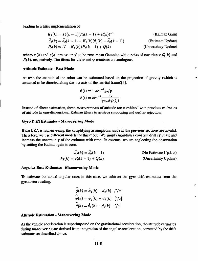
Figure 4: Drift Estimation I (Roll only)

Figure 4 shows the initialization of the drift estimate d4 while the base is at rest. Initially, the uncertainty associated with the drift estimate is high. Therefore, the drift measurements q5dS affect the drift considerably. After the drift estimates become more certain, new measurements begin to affect the drift estimates less. The computed velocity $vel quickly approaches zero.

11-9

Drift estimates during Transient

+

-3 I I I 1 I I 1 I I

550 800 850 700 750 800 850 900 950 lo00 I C =mPk

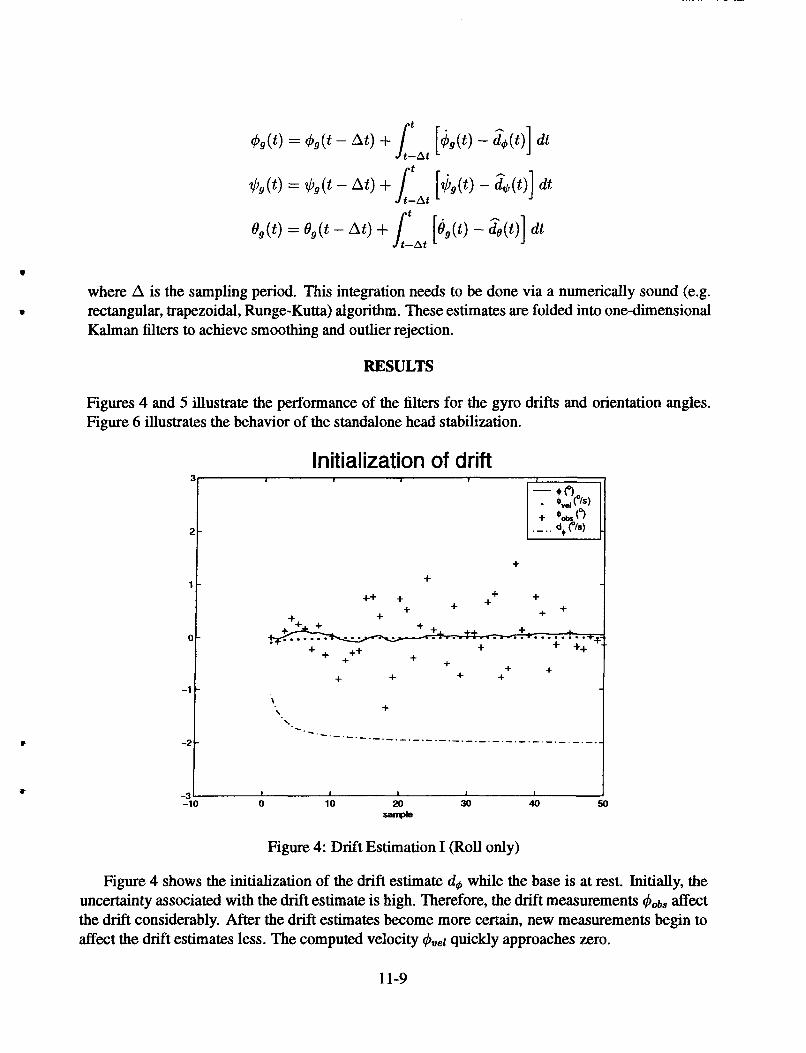
Figure 5: Drift Estimation 11 (Roll only)

io

Figure 5 illustrates both sets of Kalman filters: the orientation angles and drift estimates. After many samples, the estimate for the drift is fairly certain. Upon entering an angular transient, there is a detection lag of several samples. During this time (near sample 635) the drift estimate does not change. As described above, once a transient is detected, updates to the drift estimates are suspended for the duration of the transient. In this test, the robot begins at rest, drives over an obstacle, then is at rest again.

This filter also shows the difference in uncertainty between the at-rest observations of the atti- tude (derived from the accelerometers) and the observations derived by integrating the gyro mea- surements. The derived measurements are more precise, but are subject to a slow drift over time, while the accelerometer-derived measurements are bias-free, but have a high degree of uncertain- ty. Both types of measurements are used over time, yielding the behavior shown in Figure 5: a filter that responds quickly and accurately to measure transient behavior, but will reset the attitude estimates any time the base is at rest.

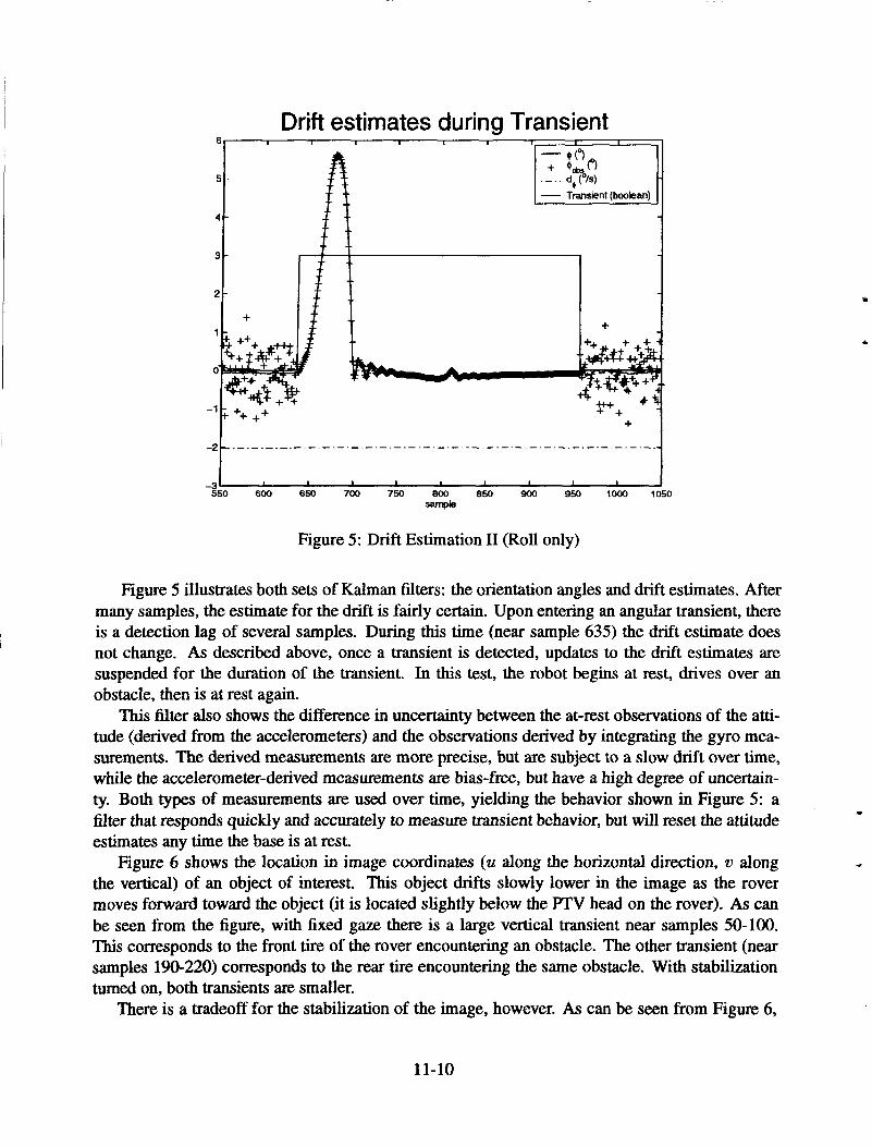
Figure 6 shows the location in image coordinates (u along the horizontal direction, 21 along the vertical) of an object of interest. This object drifts slowly lower in the image as the rover moves forward toward the object (it is located slightly below the ryTV head on the rover). As can be seen from the figure, with fixed gaze there is a large vertical transient near samples 50-100. This corresponds to the front tire of the rover encountering an obstacle. The other transient (near samples 190-220) corresponds to the rear tire encountering the same obstacle. With stabilization turned on, both transients are smaller.

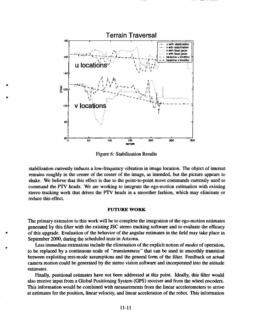
There is a tradeoff for the stabilization of the image, however. As can be seen from Figure 6,

11-10

Terrain Traversal 180 I I 1

u with stabilimiion v with stabilization

la/t-

...

.-

. . 140f

I . ..

11 S

I . .

I ... - .

Figure 6: Stabilization Results

stabilization currently induces a low-frequency vibration in image location. The object of interest remains roughly in the center of the center of the image, as intended, but the picture appears to shake. We believe that this effect is due to the point-to-point move commands currently used to command the PTV heads. We are working to integrate the ego-motion estimation with existing stereo tracking work that drives the PTV heads in a smoother fashion, which may eliminate or reduce this effect.

FUTURE WORK

The primary extension to this work will be to complete the integration of the ego-motion estimates generated by this filter with the existing JSC stereo tracking software and to evaluate the efficacy of this upgrade. Evaluation of the behavior of the angular estimates in the field may take place in September 2000, during the scheduled tests in Arizona.

Less immediate extensions include the elimination of the explicit notion of mudes of operation, to be replaced by a continuous scale of "transientness" that can be used to smoothly transition between exploiting rest-mode assumptions and the general form of the filter. Feedback on actual camera motion could be generated by the stereo vision software and incorporated into the attitude estimates.

Finally, positional estimates have not been addressed at this point. Ideally, this filter would also receive input from a Global Positioning System (GPS) receiver and from the wheel encoders. This information would be combined with measurements from the linear accelerometers to arrive at estimates for the position, linear velocity, and linear acceleration of the robot. This information

11-1 1

could be used, for example, to generate a three-dimensional path that the rover has followed.

CONCLUSION

Inertial data can be used to compensate for ego-motion in images taken from an outdoor rover. This compensation can be treated as a standalone behavior, to keep a specified object of interest centered in an image, or as an input to a more complex object tracking algorithm. Initial tests reveal that some low-frequency oscillation was introduced as a result of the stabilization, but that the amplitude of image location transients due to obstacles in the path of an outdoor rover decreased. This should expand the range of speed and surface roughness over which the rover should be able to visually track and follow a field geologist.

REFERENCES

[ 11 R. G. Brown. Introduction to Random Signal Analysis and Kalman Filtering. John Wiley & Sons, New York, 1983.

[2] C. K. Chui and G. Chen. Kalmun Filtering with Real-Time Applications. Springer-Verlag, Berlin, 1987.

[3] E. Foxlin. Inertial head-tracker sensor fusion by a complementary separate-bias k h a n filter. In Proc. 19% Krtual Reality Annual International Symposium, 1996.

[4] M. Spong and M. Vidyasagar. Robot Dynanics and Control. John Wiley & Sons, New York, 1989.

L

[5] J. Vaganay, M. J. Aldon, and A. Fournier. Mobile robot attitude estimation by fusion of inertial data. In Proceedings IEEE International Conference Robotics and Automatibn, pages 277- 282,1993.

11-12