See discussions, stats, and author profiles for this publication at: https://www.researchgate.net/publication/223603370

A comparison of neural network and linear scoring models in credit union

environment

Article  in  European Journal of Operational Research · February 1996

DOI: 10.1016/0377-2217(95)00246-4

CITATIONS

327

READS

954

3 authors:

Some of the authors of this publication are also working on these related projects:

Multi-state intensity models with random effects and B Splines View project

Energy efficient homes and mortgage risk View project

Vijay Desai

CA Technologies

16 PUBLICATIONS   564 CITATIONS   

SEE PROFILE

Jonathan Crook

The University of Edinburgh

86 PUBLICATIONS   2,316 CITATIONS   

SEE PROFILE

George Allen Overstreet

University of Virginia

46 PUBLICATIONS   647 CITATIONS   

SEE PROFILE

All content following this page was uploaded by George Allen Overstreet on 27 February 2018.

The user has requested enhancement of the downloaded file.

E L S E V I E R European Journal of Operational Research 95 (1996) 24-37

EUROPEAN JOURNAL

OF OPERATIONAL RESEARCH

T h e o r y a n d M e t h o d o l o g y

A comparison of neural networks and linear scoring models in the credit union environment

V i j a y S. D e s a i a, *, J o n a t h a n N . C r o o k b, G e o r g e A . O v e r s t r e e t , Jr. a

a Mclntire School of Commerce, University of Virginia, Charlottesville, VA 22 903, USA b Department of Business Studies, University of Edinburgh, 50 George Square, Edinburgh, EH89JY, UK

Received January 1995; revised August 1995

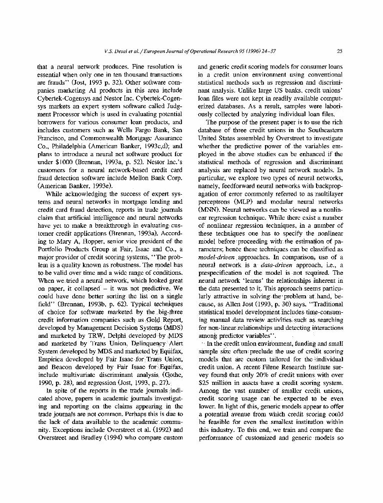
Abstract

The purpose of the present paper is to explore the ability of neural networks such as multilayer perceptrons and modular neural networks, and traditional techniques such as linear discriminant analysis and logistic regression, in building credit scoring models in the credit union environment. Also, since funding and small sample size often preclude the use of customized credit scoring models at small credit unions, we investigate the performance of generic models and compare them with customized models. Our results indicate that customized neural networks offer a very promising avenue if the measure of performance is percentage of bad loans correctly classified. However, if the measure of performance is percentage of good and bad loans correctly classified, logistic regression models are comparable to the neural networks approach. The performance of generic models was not as good as the customized models, particularly when it came to correctly classifying bad loans. Although we found significant differences in the results for the three credit unions, our modular neural network could not accommodate these differences, indicating that more innovative architectures might be necessary for building effective generic models.

Keywords: Neural networks; Banking; Credit scoring

1. Introduction

Recent issues of trade publications in the credit and banking area have published a number of articles heralding the role of artificial intelligence (AI) tech- niques in helping bankers make loans, develop mar- kets, assess creditworthiness and detect fraud. For example, HNC Inc., considered a leader in neural

* Corresponding author.

network technology, offers, among other things, products for credit card fraud detection (Falcon), automated mortgage underwriting (Colleague), and automated property valuation. Clients for HNC' s Falcon software include AT & T Universal Card, Household Credit Services, Colonial National Bank, First USA Bank, First Data Resources, First Chicago Corp., Wells Fargo & Co., and Visa International (American Banker, 1994a,b; 1993a,b). According to Allen Jost, the director of Decision Systems for HNC Inc., "Traditional techniques cannot match the fine resolution across the entire range of account profiles

0377-2217/96/$15.00 Copyright © 1996 Elsevier Science B.V. All rights reserved SSDI 0377-2217(95)00246-4

V.S. Desai et a l . / European Journal of Operational Research 95 (1996) 24-37 25

that a neural network produces. Fine resolution is essential when only one in ten thousand transactions are frauds" (Jost, 1993 p. 32). Other software com- panies marketing AI products in this area include Cybertek-Cogensys and Nestor Inc. Cybertek-Cogen- sys markets an expert system software called Judg- ment Processor which is used in evaluating potential borrowers for various consumer loan products, and includes customers such as Wells Fargo Bank, San Francisco, and Commonwealth Mortgage Assurance Co., Philadelphia (American Banker, 1993c,d); and plans to introduce a neural net software product for under $1000 (Brennan, 1993a, p. 52). Nestor Inc. 's customers for a neural network-based credit card fraud detection software include Mellon Bank Corp. (American Banker, 1993e).

While acknowledging the success of expert sys- tems and neural networks in mortgage lending and credit card fraud detection, reports in trade journals claim that artificial intelligence and neural networks have yet to make a breakthrough in evaluating cus- tomer credit applications (Brennan, 1993a). Accord- ing to Mary A. Hopper, senior vice president of the Portfolio Products Group at Fair, Isaac and Co., a major provider of credit scoring systems, "The prob- lem is a quality known as robustness, The model has to be valid over time and a wide range of conditions. When we tried a neural network, which looked great on paper, it collapsed - it was not predictive. We could have done better sorting the list on a single field" (Brennan, 1993b, p. 62). Typical techniques of choice for software marketed by the big-three credit information companies such as Gold Report, developed by Management Decision Systems (MDS) and marketed by TRW, Delphi developed by MDS and marketed by Trans Union, Delinquency Alert System developed by MDS and marketed by Equifax, Empirica developed by Fair Isaac for Trans Union, and Beacon developed by Fair Isaac for Equifax, include multivariate discriminant analysis (Gothe, 1990, p. 28), and regression (Jost, 1993, p. 27).

In spite of the reports in the; trade journals indi- cated above, papers in academic journals investigat- ing and reporting on the claims appearing in the trade journals are not common. Perhaps this is due to the lack of data available to the academic commu- nity. Exceptions include Overstreet et al. (1992) and Overstreet and Bradley (1994) who compare custom

and generic credit scoring models for consumer loans in a credit union environment using conventional statistical methods such as regression and discrimi- nant analysis. Unlike large US banks, credit unions' loan files were not kept in readily available comput- erized databases. As a result, samples were labori- ously collected by analyzing individual loan files.

The purpose of the present paper is to use the rich database of three credit unions in the Southeastern United States assembled by Overstreet to investigate whether the predictive power of the variables em- ployed in the above studies can be enhanced if the statistical methods of regression and discriminant analysis are replaced by neural network models. In particular, we explore two types of neural networks, namely, feedforward neural networks with backprop- agation of error commonly referred to as multilayer perceptrons ( M L P ) a n d modular neural networks (MNN). Neural networks can be viewed as a nonlin- ear regression technique. While there exist a number of nonlinear regression techniques, in a number of these techniques one has to specify the nonlinear model before proceeding wi th the estimation of pa- rameters; hence these techniques can be classified as model-driven approaches. In comparison, use of a neural network is a data-driven approach, i.e,, a prespecification o f the model is not required. The neural network: qearns' the relationships inherent in the data presented to it. This approach seems particu- larly attractive in solving t hep rob l em a t hand, be- cause, a s Allen Jost (1993, p, 30)says , "Traditional statistical model development includes time-consum- ing manual data review activities such as searching for non-linear relationships and detecting interactions among predictor variables".

In the credit: union environment, funding and small sample size often preclude the use of credit scoring models that are custom tailored for the:individual credit union. A recent Filene Research Institute sur- vey found that only 20% of Credit unions with over $25 million in assets have a credit scoring system. Among the vast number of smaller credit unions, credi t scoring usage can be expected to be even lower. In light of this, generic models appear to offer a potential avenue from which credit scoring could be feasible for even the smallest institution within this industry. To this end, we train and compare the performance of customized and generic models so

26 V.S. Desai et a l . / European Journal of Operational Research 95 (1996) 24-37

that the costs and benefits of the two approaches can be evaluated.

Proponents of customized models argue that credit unions enjoy very narrow fields of membership, normally employment related, and hence individual credit unions differ markedly from each other. For example, one credit union included in the present study consists of teachers whereas another one con- sists of telephone company employees. Thus, generic models would miss important differences among in- dividual credit unions. If indeed there are differences in the data representing the different credit unions, one way to detect these differences and take advan- tage of them would be to use modular neural net- works, a network architecture consisting of a multi- plicity of networks competing with each other to learn various segments of the input data space. Thus, we train and compare the performance of modular neural network models with the generic and cus- tomized neural networks as well as models based upon linear discriminant analysis and logistic regres- sion.

A comparison of the neural network models with linear discriminant analysis and logistic regression suggests that, in terms of correctly classifying good and bad loans, the neural network models outperform linear discriminant analysis, but are only marginally better than logistic regression models. However, in terms of correctly classifying bad loans, the neural network models outperform both conventional tech- niques. Since bad loans are only a small proportion of the total loans made, this result resonates with the claim made by Allen Jost of HNC Inc. that tradi- tional techniques cannot match the fine resolution produced by neural nets. In comparing generic and customized models we found that the customized models perform significantly better than generic models. However, the performance of modular neu- ral networks was not significantly better than the generic neural network model, suggesting that per- haps the differences between the individual credit unions are not that important.

In Section 2 and Section 3 we review conven- tional statistical techniques and neural network mod- els respectively; Section 4 describes the data, the sources of data, and provides the specifics of the neural networks used; Section 5 presents the results of our experiments, and Section 6 presents the con- clusions and suggestions for future research.

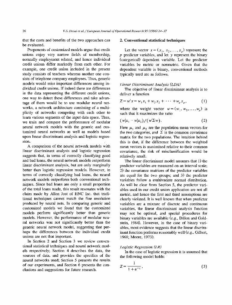
2. Conventional statistical techniques

Let the vector x = (x l, x 2 . . . . . Xp) represent the p predictor variables, and let y represent the binary (categorical) dependent variable. Let the predictor variables be metric or nonmetric. Given that the dependent variable is binary, conventional methods typically used are as follows.

Linear Discriminant Analysis (LDA) The objective of linear discriminant analysis is to

deliver a function

Z = w t x = W l X 1 -~- w 2 x 2 -~ • • • - ~ W p X p , (1)

where the weight vector w = ( w 1, w e . . . . . Wp) is such that it maximizes the ratio

- (2) Here /z I and /z 2 are the population mean vectors for the two categories, and ~ is the common covariance matrix for the two populations. The intuition behind this is that, if the difference between the weighted mean vectors is maximized relative to their common covariance, the risk of misclassification would be relatively small.

The linear discriminant model assumes that 1) the predictor variables are measured on an interval scale; 2) the covariance matrices of the predictor variables are equal for the two groups; and 3) the predictor variables follow a multivariate normal distribution. As will be clear from Section 5, the predictor vari- ables used in our credit union application are not all metric, and hence the first and third assumptions are clearly violated. It is well known that when predictor variables are a mixture of discrete and continuous variables, the linear discriminant analysis function may not be optimal, and special procedures for binary variables are available (e.g., Dillon and Gold- stein, 1984). However, in the case of binary vari- ables, most evidence suggests that the linear discrim- inant function performs reasonably well (e.g., Gilbert, 1968; Moore, 1973).

Logistic Regression (LR) In the case of logistic regression it is assumed that

the following model holds:

1 Z = 1 + e -z ' (3)

VS. Desk et al./European Journal of Operational Research 95 (1996) 24-37 27

where Z = The probability of class outcome. z = wa + w,x, + wzx* + . . . +w,x,.

The logistic regression model does not require the assumptions necessary for the linear discriminant problem. In fact, Harrell and Lee (1985) found that even when the assumptions of LDA are satisfied, LR is almost as efficient as LDA. One advantage of

LDA is that ordinary least-squares procedures can be used to estimate the coefficients of the linear dis-

criminant function, whereas maximum-likelihood methods are required for the estimation of a logistic regression model. However, given the availability of high speed computers today, computational simplic- ity is no longer considered to be an adequate crite- rion for choosing a method. A second advantage of discriminant analysis over logistic regression is that prior probabilities and misclassification costs can be easily incorporated into the LDA model. Misclassifi- cation costs and prior probabilities can also be incor- porated into neural networks (e.g., Tam and Kiang, 1992); however, since we want the results of the three methods to be comparable, the present study does not incorporate misclassification costs into the models studied. The LDA model did use the propor- tion of good and bad loans in the training samples as prior probabilities.

3. Neural networks

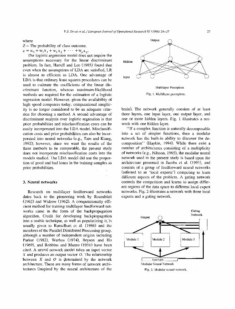
Research on multilayer feedforward networks dates back to the pioneering work by Rosenblatt (1962) and Widrow (1962). A computationally effi- cient method for training multilayer feedforward net- works came in the form of the backpropagation algorithm. Credit for developing backpropagation into a usable technique, as well as popularizing it, is usually given to Rumelhart et al. (1986) and the members of the Parallel Distributed Processing group, although a number of independent origins including Parker (19821, Werbos (19741, Bryson and Ho (19691, and Robbins and Munro (1951) have been cited. A neural network model takes an input vector X and produces an output vector 0. The relationship between X and 0 is determined by the network architecture. There are many forms of network archi- tectures (inspired by the neural architecture of the

Output n

Hidden

Input

Multilayer Perceptron

Fig. 1. Multilayer perceptron.

brain). The network generally consists of at least

three layers, one input layer, one output layer, and one or more hidden layers. Fig. 1 illustrates a net- work with one hidden layer.

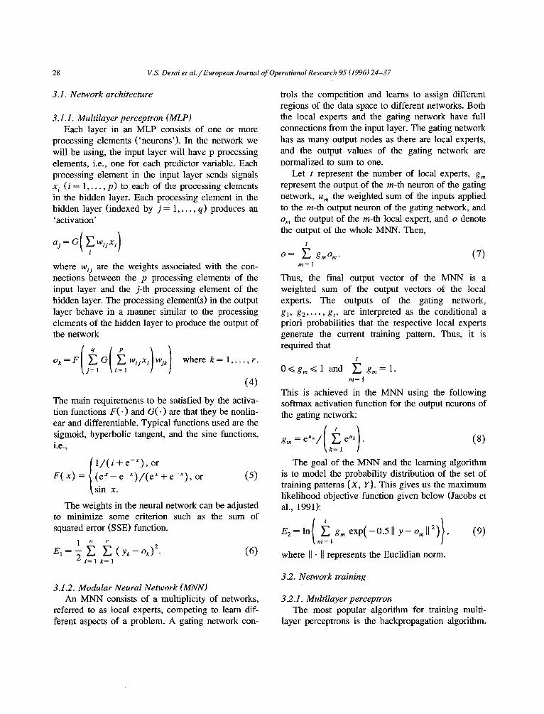
“If a complex function is naturally decomposable into a set of simpler functions, then a modular network has the built-in ability to discover the de- composition’ ’ (Haykin, 1994). While there exist a number of architectures consisting of a multiplicity of networks (e.g., Nilsson, 1965), the modular neural network used in the present study is based upon the architecture presented in Jacobs et al. (1991), and consists of a group of feedforward neural networks (referred to as ‘local experts’) competing to learn different aspects of the problem. A gating network controls the competition and learns to assign differ- ent regions of the data space to different local expert networks. Fig. 2 illustrates a network with three local experts and a gating network.

output 0

Gating Network

Modular Neural Network

Fig. 2. Modular neural network.

28 V.S. Desai et a l . / European Journal of Operational Research 95 (1996) 24-37

3.1. Network architecture

3.1.1. Multilayer perceptron (MLP) Each layer in an MLP consists of one or more

processing elements ( 'neurons'). In the network we will be using, the input layer will have p processing elements, i.e., one for each predictor variable. Each processing element in the input layer sends signals x i (i = 1 . . . . . p) to each of the processing elements in the hidden layer. Each processing element in the hidden layer (indexed by j = 1 . . . . . q) produces an 'activation'

aj=G( ~i wijxi )

where wij are the weights associated with the con- nections between the p processing elements of the input layer and the j-th processing element of the hidden layer. The processing element(s) in the output layer behave in a manner similar to the processing elements of the hidden layer to produce the output of the network

o k = F G ~_.wijx i w~k where k = l . . . . . r. i = l

(4)

The main requirements to be satisfied by the activa- tion functions F ( - ) and G(-) are that they be nonlin- ear and differentiable. Typical functions used are the sigmoid, hyperbolic tangent, and the sine functions, i.e.,

' l / ( i + e - X ) , o r F(x ) = (e x - e -X) / (e x + e-X), or (5)

sin x.

The weights in the neural network can be adjusted to minimize some criterion such as the sum of squared error (SSE) function.

lkk = ( yk - 0 0 2 . (6 )

l = l k = l

3.1.2. Modular Neural Network (MNN) An MNN consists of a multiplicity of networks,

referred to as local experts, competing to learn dif- ferent aspects of a problem. A gating network con-

trois the competition and learns to assign different regions of the data space to different networks. Both the local experts and the gating network have full connections from the input layer. The gating network has as many output nodes as there are local experts, and the output values of the gating network are normalized to sum to one.

Let t represent the number of local experts, g,, represent the output of the m-th neuron of the gating network, u m the weighted sum of the inputs applied to the m-th output neuron of the gating network, and o,, the output of the m-th local expert, and o denote the output of the whole MNN. Then,

t

O = E groOm • ( 7 ) m = l

Thus, the final output vector of the MNN is a weighted sum of the output vectors of the local experts. The outputs of the gating network, gl, g2 . . . . . gt, are interpreted as the conditional a priori probabilities that the respective local experts generate the current training pattern. Thus, it is required that

t

O <~ gm <~ l and ~ gm = l. m = l

This is achieved in the MNN using the following softmax activation function for the output neurons of the gating network:

g , . = e " ~ / e u* . ( 8 )

The goal of the MNN and the learning algorithm is to model the probability distribution of the set of training patterns {X, Y}. This gives us the maximum likelihood objective function given below (Jacobs et al., 1991):

E2 =ln( ~ gm exp(-O'5ll Y - ° " ] ' 2 ) ) (9)

where I1" II represents the Euclidian norm.

3.2. Network training

3.2.1. Multilayer perceptron The most popular algorithm for training multi-

layer perceptrons is the backpropagation algorithm.

V.S. Desai et al./ European Journal of Operational Research 95 (1996) 24-37 29

As the name suggests, the error computed from the output layer is backpropagated through the network, and the weights are modified according to their contribution to the error function. Essentially, back- propagation performs a local gradient search, and hence its implementation, although not computation- ally demanding, does not guarantee reaching a global minimum. A number of heuristics are available to alleviate this problem, some of which are presented below.

Let x~ ~] be the current output of the j-th neuron in layer s, I~ s] the weighted summation of the inputs to the i-th neuron in layer s, f ' ( l [ ~J) the derivative of the activation function of the i-th neuron in layer s, and elk s] the local error of the k-th neuron in layer s. Then, after some mathematical simplification (e.g., see Haykin, 1994, pp. 144-152) the weight change equation suggested by backpropagation and (6) can be expressed as follows:

AWl; ] = ~ f t ( i:s]) E ( elk s+ l]Wki)X~ s - 1] ..1_ OAwij. k

(lO)

for non-output layers, and

AWl} ] = 7"1( Yi -- o i ) f ' ( l i ) x ~ s- l] "b OmWij. ( 1 1 )

for the output layer. Here 7/ is the learning coeffi- cient, and 0 is the momentum term. One heuristic that is used to prevent the network from getting stuck at a local minimum is random presentation of the training data (e.g., Haykin 1994, pp. 149-150.) In the absence of the second term in (10) and (11), setting a low learning coefficient results in slow learning, whereas a high learning coefficient can produce divergent behavior. The second term in (10) and (11) reinforces general trends whereas oscilla- tory behavior is canceled out, thus allowing a low learning coefficient but faster learning. Last, it is suggested that starting the training with a large learn- ing coefficient and letting its value decay as training progresses speeds up convergence, All these heuris- tics have been used in the models studied in the current paper.

There are three criteria that are commonly used to stop network training, namely, after a fixed number of iterations, or after the error reaches a certain prespecified minimum, or after the network reaches a fairly stable state and learning effectively ceases. In

the current paper we allowed the network to run for a maximum of 100000 iterations. Training was stopped before 100000 iterations if the error crite- rion (E 1 defined in (6)) reached below 0.1. Also, the percentage of training patterns correctly classified was checked after every cycle of 1000 iterations and the network saved if there was an improvement over the previous best saved network. Thus, the network used on the test data set was the one that had shown the best performance on the training data set during a training of up to 100,000 iterations. The same crite- ria were also used for the MNN described below.

3.2.2. Modular neural network Like the MLP, training in MNN is also done

using the backpropagation of error. Training of the local experts and the gating network can occur si- multaneously, or each local expert can be trained in a hierarchical fashion. The learning rule is designed to encourage competition among the local experts so that, for a given input vector, the gating network will tend to choose a single local expert rather than a mixture o f them. In this way the input space is automatically partitioned into regions so that each local expert takes responsibility for a different re- gion.

Given (9), after some mathematical simplification (e.g., Haykin, 1994, pp. 482-487) the modif ied weight change equations for the output layers of the local experts and the gating network can be ex- pressed as follows:

Aw!; l --- r lh i (Y i - - o i ) f ' ( t i ) x ~ s- '] + OAwij (12)

for local expert, and

Aw~; ] --- r/( hi-- gi) x~ s- '1 + OAwij (13)

for the gating network, where

gi exp( - 0.5 II Y -- oi [12 )

h i = ~_,tm=lg m exp(-0.511 y - o , , t l 2 ) " (14)

h i can be interpreted as the posterior probability that the i-th local expert is responsible for the current output vector.

3.3. Network size

Important questions about network size that need to be answered are as follows: one, how does one

30 V.S. Desai et a l . / European Journal of Operational Research 95 (1996) 24-37

determine the number of processing elements in the hidden layer, and second, how many hidden layers are adequate? As yet there are no firm answers for these questions; however, certain heuristics are avail- able. A higher number of processing elements will lead to a greater flexibility on the part of the network to fit the data. However, this need not necessarily be good because then the network will not only capture the information content of the data but will also learn the error in the data, and hence will not be very useful for the purpose of generalization or prediction. As for the second question, theoretically, a single hidden layer should be sufficient, but the training time required with a single hidden layer may be very high. Addition of a second hidden layer may reduce the training time.

In stepwise regression, one can start with a small number of variables and add the most significant variable (forward selection) one by one, or one can start with a large number of variables and eliminate the least significant variable (backward elimination) one by one. Criteria to select best subsets of regres- sors are also available. Equivalent strategies in neu- ral networks modeling have been explored. For ex- ample, the cascade correlation network (Fahlman and Lebierre, 1990) starts with zero neurons in the hid- den layer and adds one neuron at a time to the hidden layer till the error criterion is satisfied or the performance stops improving. Alternatively, one can start with a network with a large number of neurons and eliminate neurons. It has been suggested that "starting with oversized networks rather than with tight networks seems to make it easier to find a good solution" (Weigend et al., 1990). One then tackles the problem of overfitting by somehow eliminating the excess neurons. While a number of methods for eliminating the excess neurons have been explored, a method that seems to be readily applicable in our case is given below.

3.3.1. Network pruning The hypothesi s that " . . . the simplest most robust

network which accounts for a data set will~ on average, lead to the best generalization to the popula- tion from which the training set has been drawn" was made by Rumelhart (reported in Hanson and Pratt, 1988). One of the simplest implementations of this hypothesis is to check the network at periodic

intervals and eliminate a certain maximum number of nodes in the hidden layers if the elimination does not lead to a significant deterioration in performance. We implemented this hypothesis in our current paper as follows. As mentioned above each network was trained for up to 100000 iterations. The following procedure was used after every cycle of 1000 itera- tions to check whether one or more of the processing elements could be permanently disabled:

(a) Find the percentage of the training data set correctly classified to determine a 'reference' level of performance.

(b) Disable the processing element by setting its output to 1.0.

(c) If the percentage of the training data set correctly classified did not drop below 75% of the 'reference' level the processing element was added to the 'candidate' prune list.

(d) Disable the processing element by setting its output to 0.0.

(e) If the percentage of the training data set correctly classified did not drop below 75% of the 'reference' level the processing element was added to the 'candidate' prune list.

(f) Re-enable the the processing element and con- tinue with the next one.

(g) Sort the 'candidate' prune list in the order of performance and disable the top two candidates by setting their output to zero.

4. Data sample and model construction

4.1. Data sample

As mentioned earlier, unlike large banks, credit unions' loan files were not kept in readily available computerized databases. Consequently samples had to be laboriously collected by analyzing individual loan files. Data were collected from the loan files of three credit unions in the Southeastern United States for the period 1988 through 1991. Credit union L is predominantly made up of teachers and credit union M is predominantly made up of telephone company employees, whereas credit union N represents a more diverse state-wide sample. The narrowness of mem- bership is somewhat mitigated by the inclusion of family members in all three credit unions. Only

V.S. Desai et al . / European Journal of Operational Research 95 (1996) 24-37 31

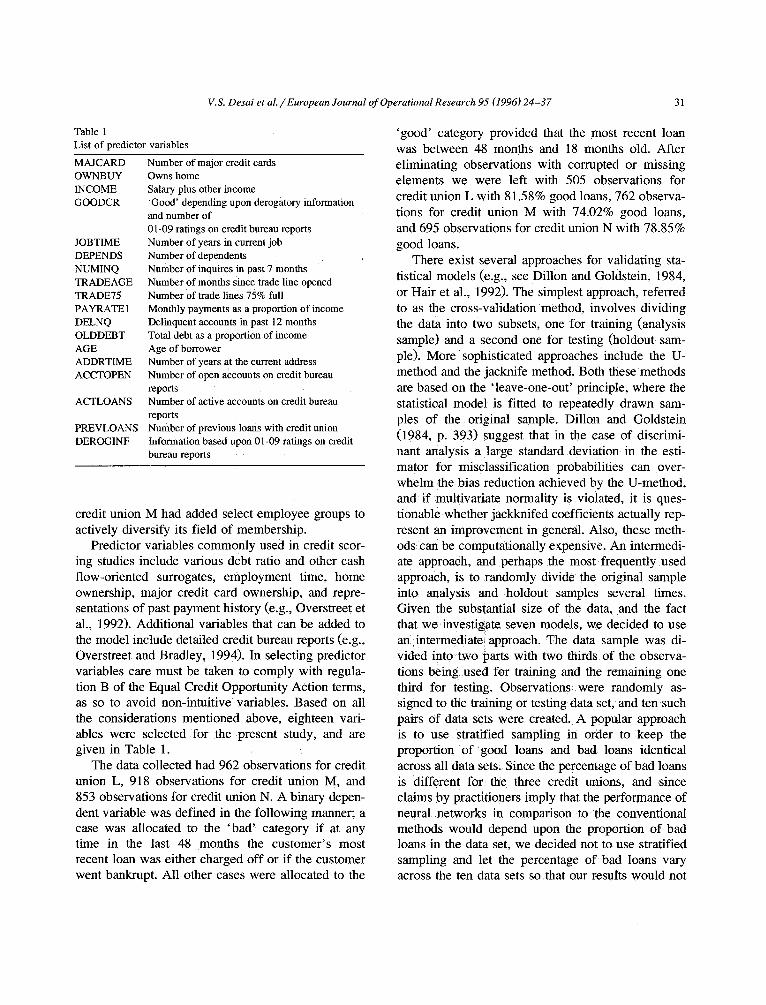
Table 1 List of predictor variables

MAJCARD OWNBUY INCOME GOODCR

JOBTIME DEPENDS NUMINQ TRADEAGE TRADE75 PAYRATE 1 DELNQ OLDDEBT AGE ADDRTIME ACCTOPEN

ACTLOANS

PREVLOANS DEROGINF

Number of major credit cards Owns home Salary plus other income 'Good' depending upon derogatory information and number of 01-09 ratings on credit bureau reports Number of years in current job Number of dependents Number of inquires in past 7 months Number of months since trade line opened Number of trade lines 75% full Monthly payments as a proportion of income Delinquent accounts in past 12 months Total debt as a proportion of income Age of borrower Number of years at the current address Number of open accounts on credit bureau reports Number of active accounts on credit bureau reports Number of previous loans with credit union Information based upon 01-09 ratings on credit bureau reports

credit union M had added select employee groups to actively diversify its field o f membership.

Predictor variables commonly used in credit scor- ing studies include various debt ratio and other cash f low-oriented surrogates, employment time, home ownership, major credit card ownership, and repre- sentations of past payment history (e.g., Overstreet et al., 1992). Addi t ional variables that can be added to the model include detailed credit bureau reports (e.g., Overstreet and Bradley, 1994). In selecting predictor variables care must be taken to comply with regula- tion B of the Equal Credit Opportunity Act ion terms, as so to avoid non-intuit ive variables. Based on all the considerations ment ioned above, eighteen vari- ables were selected for the p resen t s tudy, and are given in Table 1.

The data collected had 962 observations for credit union L, 918 observations for credit union M, and 853 observations for credit union N. A binary depen- dent variable was defined in the fol lowing manner; a case was al located to the ' b a d ' category if at any time in the last 48 months the cus tomer ' s most recent loan was either charged off or if the customer went bankrupt. All other cases were al located to the

' good ' category provided that the most recent loan was between 48 months and 18 months old. After el iminating observations with corrupted or missing elements we were left with 505 observations for credit union L with 81.58% good loans, 762 observa- tions for credit union M with 74.02% good loans, and 695 observations for credit union N with 78.85% good loans.

There exist several approaches for validating sta- tistical models (e.g., see Dillon and Goldstein, 1984, or Hair et al., 1992). The simplest approach, referred to as the cross-validation method, involves dividing the data into two subsets, one for training (analysis sample) and a second one for testing (holdout sam- ple). More sophisticated approaches include the U- method and the jacknife method. Both these methods are based on the ' leave-one-out ' principle, where the statistical model is fitted to repeatedly drawn sam- ples of the original sample. Dil lon and Goldstein (1984, p. 393) suggest that in the case o f discrimi- nant analysis a large standard deviation in the esti- mator for misclassification probabili t ies can over- whelm the bias reduction achieved by the U-method, and i f multivariate normali ty is violated, it is ques- t ionable whether jackknifed coefficients actually rep- resent an improvement in general. Also, these meth- ods can be computat ionally expensive, An intermedi- ate approach, and perhaps the most frequently used approach, is t o randomly divide the original sample into analysis and holdout samples several times. Given the substantial size of the data, and the fact that we investigate seven models, we decided to use an in termedia te approach. The data sample was di- vided into two parts with two thirds of the observa- tions being used for training and the remaining one third for testing. Observations were randomly as- signed to the training or testing data set, and ten such pairs of data sets were created. A popular approach is to use stratified sampling in order to k e e p the proport ion of good loans and bad loans identical across all data sets. Since the percentage of bad loans is different for the three credit unions, and since claims by practit ioners imply that the performance of neural networks in comparison to the conventional methods would depend upon the proport ion o f bad loans in the data set, we decided not to use stratified sampling and let the percentage of bad loans vary across the ten data sets so tha t our results would not

32 V.S. Desai et a l . / European Journal of Operational Research 95 (1996) 24-37

be dependent upon the particular composition of the data sample at hand. As Section 5 indicates when the results were compared, we accounted for this varia- tion by performing paired t-tests. The data sets for the generic models were created by merging the data sets for the individual credit unions.

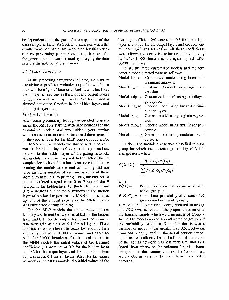
4.2. Model construction

As the preceding paragraphs indicate, we want to use eighteen predictor variables to predict whether a loan will be a 'good' loan or a 'bad' loan. This fixes the number of neurons in the input and output layers to eighteen and one respectively. We have used a sigmoid activation function in the hidden layers and the output layer, i.e.,

F(z) = 1/ (1 + e-Z).

After some preliminary testing we decided to use a single hidden layer starting with nine neurons for the customized models, and two hidden layers starting with nine neurons in the first layer and three neurons in the second layer for the MLP generic models. For the MNN generic models we started with nine neu- rons in the hidden layer of each local expert and six neurons in the hidden layer of the gating network. All models were trained separately for each of the 10 samples for each credit union. Also, note that due to pruning the models at the end of training did not have the same number of neurons as some of them were eliminated due to pruning. Thus, the number of neurons deleted ranged from 0 to 7 out of the 9 neurons in the hidden layer for the MLP models, and 0 to 4 neurons out of the 9 neurons in the hidden layer of the local experts of the MNN models. Also, up to 1 of the 3 local experts in the MNN models was eliminated during training.

For the MLP models the initial values of the learning coefficient (r/) were set at 0.3 for the hidden layer and 0.15 for the output layer, and the momen- tum term (0) was set at 0.4 for all layers. These coefficients were allowed to decay by reducing their values by half after 10000 iterations, and again by half after 30 000 iterations. For the local experts in the MNN models the initial values of the learning coefficient (~7) were set at 0.9 for the hidden layer and 0.6 for the output layer, and the momentum term (0) was set at 0.4 for all layers. Also, for the gating network in the MNN models, the initial values of the

learning coefficient (~7) were set at 0.3 for the hidden layer and 0.075 for the output layer, and the momen- tum term (0) was set at 0.4. All these coefficients were allowed to decay by reducing their values by half after 10000 iterations, and again by half after 30 000 iterations.

In all, the three customized models and the four generic models tested were as follows: Model lda_c: Customized model using linear dis-

criminant analysis. Model lr_ c: Customized model using logistic re-

gression. Model mlp_c: Customized model using multilayer

perceptron. Model lda_ g: Generic model using linear discrimi-

nant analysis. Model lr_ g: Generic model using logistic regres-

sion. Model mlp_ g: Generic model using multilayer per-

ceptron. Model m n n g: Generic model using modular neural

network. In the LDA models a case was classified into the

group for which the posterior probability P(Gj[Z) was greatest, where

P(ZIGj)P(Gj) p( jlz) = 2

E p(zL c,)P(a/) i=1

with: P(G~) = Prior probability that a case is a mem-

ber of group j. P(ZI Gj) = Conditional probability of a score of Z,

given membership of group j. Here Z is the discriminant score generated using (1), and P(Gj) was set equal to the proportion of cases in the training sample which were members of group j. In the LR models a case was allocated to group j if the probability (equal to Z in (3)) that it was a member of group j was greater than 0.5. Following Tam and Kiang (1992), in the neural networks mod- els a case was allocated as a 'bad' loan if the output of the neural network was less than 0.5, and as a 'good' loan otherwise, the rationale for this scheme being that in the training data set the 'good' loans were coded as ones and the 'bad' loans were coded as zeros.

V.S. Desai et al. / European Journal of Operational Research 95 (1996) 24-37 33

4.3. Computational experience

The LR and LDA models were implemented on a Sequent $2000/750 machine with eighteen 386 and 486 processors, using SPSS version 6.0. The pro- gram was probably run on a single 20 MHz 386 processor. The CPU seconds required for training each sample ranged from 4 to 25 seconds for LDA models and 7 to 65 seconds for LR models. The MLP and MNN models were run on an IBM P S / 2

machine with a 33 MHz 486 processor, using Neu- ralWorks Professional H/Plus. The real time re- quired for training each sample ranged from 300 to 900 seconds.

5. Comparison of results

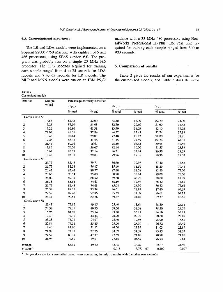
Table 2 gives the results of our experiments for the customized models, and Table 3 does the same

Table 2 Customized models

Data set Sample % bad

Percentage correctly classified

mlp_ c Ida_ c lr_ c

% total % bad % total % bad % total % bad

Credit union L" 1 14.88 83.33 32.00 83.30 16.00 82.70 24.00 2 17.26 87.50 31.03 82.70 20.69 81.00 34.48 3 17.26 86.90 41.38 83.90 31.03 82.10 37.93 4 22.02 81.55 37.84 84.52 32.43 82.74 37.84 5 18.45 82.14 29.03 77.40 16.13 78.00 38.71 6 17.26 83.33 41.38 • 81.55 27.59 82.74 41.38 7 21.43 80.36 16.67 78.50 08.33 80.95 30.56 8 17.86 79.76 56.67 82.14 10.00 81.55 23.33 9 16.67 85.71 32.14 86.31 32.14 86.90 39.29

10 18.45 83.33 29~03 79.76 19.35 80.36 29.03 Credit union M: 1 26.77 85.43 79.71 86.60 70.97 87.40 73.53 2 26.77 88.58 76.47 85.40 18.64 88.20 79.41 3 20.47 85.43 80.77 87.40 31.58 85.80 75.00 4 23.63 90.94 75.00 90.20 35.14 89.00 75.00 5 24.02 89.37 88.52 89.80 22.22 88.60 81.97 6 26.38 88.58 74.63 88.19 12.96 86.22 71.64 7 26.77 85.43 74.63 85.04 28.30 86.22 77.61 8 25.59 88.19 75.38 86.61 28.89 87.40 67.69 9 27.59 87.40 72.86 85.43 31.37 86.61 67.14

10 24.41 90.55 82.26 89.37 21.05 89.37 80.65 Credit union N: 1 25.43 75.86 49.15 75.40 18.64 78.50 27.11 2 24.57 77.15 40.35 78.50 31.58 78.50 24.56 3 15.95 81.90 35.14 83.20 35.14 84.10 35.14 4 19.40 77.15 44.44 78.90 22.22 80.60 28.89 5 23.28 76.72 24.07 75.40 12.96 75.90 18.52 6 22.84 79.31 35.85 75.00 28.30 76.72 26.42 7 19.40 81.90 31.11 80.60 28.89 81.03 28.89 8 21.98 74.13 37.25 74.57 31.37 75.43 31.37 9 24.57 80.17 47.37 77.59 21.05 78.88 21.05

I 0 21.98 77.59 19.61 77.16 21.57 76.72 19.61

average 83.19 49.72 82.35 38.49 82.67 44.93 p-value a 0.018 5.7E - 07 0.109 0.007

a The p-values are for a one-tailed paired t-test comparing the mlp_ c results with the other two methods.

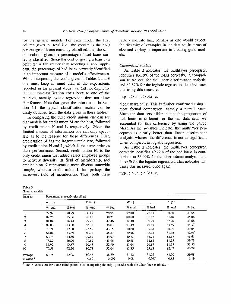
34 V.S. Desai et al . / European Journal of Operational Research 95 (1996) 24-37

for the generic models. For each model the first column gives the total (i.e., the good plus the bad) percentage of loans correctly classified, and the sec- ond column gives the percentage of bad loans cor- rectly classified. Since the cost of giving a loan to a defaulter is far greater than rejecting a good appli- cant, the percentage of bad loans correctly identified is an important measure of a model 's effectiveness. While interpreting the results given in Tables 2 and 3 one must keep in mind that, in the experiments reported in the present study, we did not explicitly include misclassification costs because one of the methods, namely logistic regression, does not allow that feature. Note that given the information in Sec- tion 4.1, the typical classification matrix can be easily obtained from the data given in these tables.

In comparing the three credit unions one can see that models for credit union M are the best, followed by credit union N and L respectively. Given the limited amount of information one can only specu- late as to the reasons for these differences. First, credit union M has the largest sample size, followed by credit union N and L, which is the same order as their performance. Second, credit union M is the only credit union that added select employee groups to actively diversify its field of membership, and credit union N represents a more diverse statewide sample, whereas credit union L has perhaps the narrowest field of membership. Thus, both these

factors indicate that, perhaps as one would expect, the diversity of examples in the data set in terms of size and variety is important in creating good mod- els.

Customized models As Table 2 indicates, the multilayer perceptron

identifies 83.19% of the loans correctly, in compari- son to 82.35% for the linear discriminant analysis, and 82.67% for the logistic regression. This indicates that using this measure,

mlp_ c > lr_ c > Ida_ c,

albeit marginally. This is further confirmed using a more formal comparison, namely a paired t-test. Since the data sets differ in that the proportion of bad loans is different for the ten data sets, we accounted for this difference by using the paired t-test. As the p-values indicate, the multilayer per- ceptron is clearly better than linear discriminant analysis, whereas the difference is not as significant when compared to logistic regression.

As Table 2 indicates, the multilayer perceptron correctly identifies 49.72% of the bad loans in com- parison to 38.49% for the discriminant analysis, and 44.93% for the logistic regression. This indicates that using this measure, once again,

mlp_ c > lr_ c > Ida_ c.

Table 3 Generic models

Data set Percentage correctly classified

mlp_ g mnn_ g Ida_ g lr_ g

% total % bad % total % bad % total % bad % total % bad

1 79.97 28.29 8 0 . 1 2 28,95 79.80 27.63 80.30 33.55 2 82.26 35.06 81.80 38.31 80.60 31.82 81.40 35.06 3 81.04 36.44 79.20 47.46 82.40 37.29 82.70 40.68 4 82.88 33.80 83.33 38.03 83.49 40.85 83.49 44.37 5 79.21 32.88 78.59 43.15 80.60 37.67 80.01 39.04 6 81.04 53.69 80.73 35.57 80.58 38.93 81.35 42.95 7 80.73 44.30 79.82 44.97 80.73 36.24 82.57 41.61 8 78.89 50.00 79.82 41.96 80.58 32.88 81.35 39.73 9 81.92 43.87 80.43 32.90 81.04 30.97 81.35 33.55

10 79.51 62.50 80.73 32.64 81.35 33.33 82.42 40.28

average 80.75 42.08 80.46 38.39 81.12 34.76 81.70 39.08 p-value a 0.191 0.197 0.98 0.035 0.83 0.19

a The p-values are for a one-tailed paired t-test comparing the mlp_ g results with the other three methods;

V.S. Desai et al. / European Journal o f Operational Research 95 (1996) 24-37 35

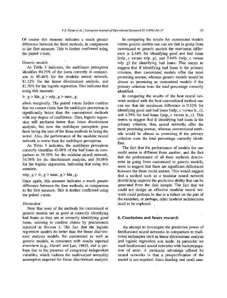
Of course this measure indicates a much greater difference between the three methods, in comparison to the first measure. This is further confirmed using the paired t-tests.

Generic models As Table 3 indicates, the multilayer perceptron

identifies 80.75% of the loans correctly in compari- son to 80.46% for the modular neural network, 81.12% for the linear discriminant analysis, and 81.70% for the logistic regression. This indicates that using this measure,

lr_ g > I d a g > mlp_ g > mnn_ g,

albeit marginally. The paired t-tests further confirm that we cannot claim that the multilayer perceptron is significantly better than the conventional methods with any degree of confidence. Thus, logistic regres- sion still performs better than linear discriminant analysis, but now the multilayer perceptron goes from being the best of the three methods to being the worst. Also, the performance of the modular neural network is worse than the multilayer perceptron.

As Table 3 indicates, the multilayer perceptron correctly identifies 42.08% of the bad loans in com- parison to 38.39% for the modular neural network, 34.76% for the discriminant analysis, and 39.08% for the logistic regression, indicating that using this measure,

mlp_g > lr_g > mnn_g > lda_g.

Once again, this measure indicates a much greater difference betweep the four methods, in comparison to the first measure. This is further confirmed using the paired t-tests.

Discussion Note that none of the methods for customized or

generic models are as good at correctly identifying bad loans as they are at correctly identifying good loans, seeming to confirm claims by practitioners reported in Section 1. The fact that the logistic regression models do better than the linear discrimi- nant analysis models, for customized as well as generic models, is consistent with results reported elsewhere (e.g., Harrell and Lee, 1985), and is per- haps due to the presence of categorical independent variables, which violates the multivariate normality assumption required for linear discriminant analysis.

In comparing the results for customized models versus generic models one can see that in going from customized to generic models the maximum differ- ence is 2.44% for identifying good and bad loans (mlp_c versus mlp_g), and 7.64% (mlp_c versus mlp_g) for identifying bad loans. This seems to suggest that if identifying bad loans is the primary criterion, then customized models offer the most promising avenue, whereas generic models would be almost as promising as customized models if the primary criterion were the total percentage correCtly identified.

In comparing the results of the best neural net- work method with the best conventional method one can see that the maximum difference is 0.52% for identifying good and bad loans (mlp_ c versus lr_ c), and 4.79% for bad loans (mlp_ c versus l r c). This seems to suggest that if identifying bad loans is the primary criterion, then neural networks offer the most promising avenue, whereas conventional meth- ods would be almost as promising if the primary criterion were the total percentage correctly identi- fied.

The fact that the performance of models for one credit union is different from another, and the fact that the performance of all three methods deterio- rates in going from customized to generic models, seem to suggest that there are significant differences between the three credit unions. This would suggest that a method such as a modular neural network should help improve the predictive ability that can be generated from the data sample. The fact that we could not design an effective modular neural net- work could perhaps be due to a failure onthe part of the modelers, or perhaps, other modular architectures need to be explored.

6. Conclusions and future research

An attempt to investigate the predictive power of feedforward neural networks in comparison to tradi- tional techniques such as linear discriminant analysis and logistic regression was made. In particular we used feedforward neural networks with backpropaga- tion of error. A particular advantage offered by neural networks is that a prespecification of the model is not required. Since funding and small sam-

36 V.S. Desai et aL / European Journal of Operational Research 95 (1996) 24-37

pie size often preclude the use of customized credit scoring models at small credit unions, we investi- gated the performance of generic models and com- pared them with customized models.

Our results indicate that customized neural net- works offer a promising avenue if the measure of performance is percentage of bad loans correctly classified. However, if the measure of performance is percentage of good and bad loans correctly classi- fied, logistic regression models are comparable to the neural networks approach. The performance of generic models was not as good as the customized models, particularly when it came to correctly classi- fying bad loans. Also, there were significant differ- ences in the results for the three credit unions, indicating that more innovative architectures might be necessary for building effective generic models, which, we believe, could be a fruitful area for future research.

Acknowledgement

Financial support from the McIntire Associates Program is gratefully acknowledged by the first au- thor.

References

American Banker (1994a), March 2, 15:1. American Banker (1994b), April 22, 17:1. American Banker (1993a), August 27, 14:4. American Banker (1993b), July 14, 3:1. American Banker (1993e), June 25, 3:1. American Banker (1993d), March 29, 15A:l. American Banker (1993e), October 5, 14:1. Brennan, P.J. (1993a), "Promise of Artificial Intelligence remains

elusive in banking today", Bank Management, July, 49-53. Brerman, P.J. (1993b), "Profitability scoring comes of age",

Bank Management, September, 58-62. Bryson, A.E., and Ho, Y.C. (1969), Applied Optimal Control,

Hemisphere, New York. Dillon, W.R., and Goldstein, M. (1984), Multivariate Analysis

Methods and Applications, Wiley, New York. Fahlman, S.E., and Lebierre, C. (1990), "The Cascade-Correla-

tion learning architecture", School of Computer Science Re- port CMU-CS-90-100, Carnegie Mellon University.

Gilbert, E.S. (1968), "On discrimination using qualitative vari- ables", Journal of the American Statistical Association 63, 1399-1412.

Gothe, P. (1990), "Credit Bureau point scoring sheds light on shades of gray", The Credit WorM, May-June, 25-29.

Hair, J.F., Anderson, R.E., Tatham, R.L., and Black, W.C. (1992), Multivariate Data Analysis: Eighth Readings, Macmillan, New York.

Hanson, S.J. and Pratt, L. (1988), "A comparison of different biases for minimal network construction with back-propa- gation", in: D.S. Touretzky (ed.) Advances in Neural Infor- mation Processing Systems I, Morgan Kanfinann, San Mateo, CA, 177-185.

Harrell, F.E., and Lee, K.L. (1985), "A comparison of the discrimination of discriminant analysis and logistic regression under multivariate normality", in: P.K. Se (ed.) Biostatistics: Statistics in Biomedical, Public Health, and Environmental Sciences, North-Holland, Amsterdam.

Haykin, S. (1994), Neural Networks: A Comprehensive Founda- tion, Macmillan, New York.

Jacobs, R.A., Jordan, M.I., Nowlan, S.J., and Hinton, G.E. (1991), "Adaptive mixtures of local experts", Neural Computation 3, 79-87.

Jost, A. (1993), "Neural networks: A logical progression in credit and marketing decision systems", Credit WorM, March/April, 26-33.

Lapedes, A., and Farber, R. (1987), "Non-linear signal processing using neural networks: Prediction and system modeling", Los Alamos National Laboratory Report LA-UR-87-2662.

Moore, D.H. (1973), "Evaluation of five discrimination proce- dures for binary variables", Journal of the American Statisti- cal Association 68, 399.

Nilsson, N.J. (1965), Learning Machines: Foundations of Train- able Pattern-Classifying Systems, McGraw-Hill, New York.

Overstreet, Jr., G.A., and Bradley, Jr., E.L. (1994), "Applicability of generic linear scoring models in the USA Credit Union environment: Further analysis", Working Paper, University of Virginia.

Overstreet, Jr., G.A., Bradley, Jr., E.L., and Kemp, R.S. (1992), "The flat-maximum effect and generic linear scoring model: A test", 1MA Journal of Mathematics Applied in Business and Industry 4, 97-109.

Parker, D.B. (1982), "Learning logic", Invention Report 581-64 (File I), Office of Technology Licensing, Stanford University.

Robbins, H., and Munro, S. (1951), "A stochastic approximation method", Annals of Mathematical Statistics 22, 400-407.

Rosenblatt, F. (1962), Principles of Neurodynamics, Spartan Books, Washington, DC.

Rumelhart, D.E. (1988), "Learning and generalization", in: Pro- ceedings of the IEEE International Conference on Neural Networks, plenary address, San Diego.

Rumelhart, D.E., Hinton, G.E., and Williams, R.J. (1986), "Learning internal representations by error propagation", in: D.E. Rumelhart and J.L. McCleland (eds.), Parallel Dis- tributed Processing: Explorations in the Microstructures of Cognition, Vol. 1, MIT Press, Cambridge, MA, 318-362.

Werhos, P. (1974), "Beyond regression: New tools for prediction and analysis in the behavioral sciences", Unpublished Ph.D. dissertation, Dept. of Applied Mathematics, Harvard Univer- sity.

V.S. Desai et aL / European Journal of Operational Research 95 (1996) 24-37 37

Widrow, B. (1962), "Generalization and information storage in networks of adaline 'neurons'", in: M.C. Yovitz, G.T. Jacobi, and G.D. Goldstein (eds.), Self-organizing Systems, Spartan Books, Washington, DC, 435-461.

Tam, K.Y., and Kiang, M.Y. (1992), "Managerial applications of

neural networks: The case of bank failure predictions", Man- agement Science 38, 926-947.

Weigend, A.S., Huberman, B.A., and Rumelhart, D.E. (1990), "Predicting the future: A connectionist approach", Working Paper, Stanford University.

View publication statsView publication stats