Euro Area Real-Time Density Forecasting

with Financial or Labor Market Frictions

Peter McAdam and Anders Warne*

February 1, 2018

Abstract: We compare real-time density forecasts for the euro area using three DSGE mod-

els. The benchmark is the Smets and Wouters model and its forecasts of real GDP growth and

inflation are compared with those from two extensions. The first adds financial frictions and

expands the observables to include a measure of the external finance premium. The second

allows for the extensive labor-market margin and adds the unemployment rate to the observ-

ables. The main question we address is if these extensions improve the density forecasts of real

GDP and inflation and their joint forecasts up to an eight-quarter horizon. We find that adding

financial frictions leads to a deterioration in the forecasts, with the exception of longer-term

inflation forecasts and the period around the Great Recession. The labor market extension

improves the medium to longer-term real GDP growth and shorter to medium-term inflation

forecasts weakly compared with the benchmark model.

Keywords: Bayesian inference, DSGE models, forecast comparison, inflation, output, predic-

tive likelihood.

JEL Classification Numbers: C11, C32, C52, C53, E37.

1. Introduction

Medium-size dynamic stochastic general equilibrium (DSGE) models—as exemplified by Smets

and Wouters (2007)—have been widely used among central banks for policy analysis, forecast-

ing and to provide a structural interpretation of economic developments; see, e.g., Del Negro

and Schorfheide (2013) and Lindé, Smets, and Wouters (2016). Recent years have, however,

constituted an especially challenging policy environment. Given the global financial crisis in

late 2008, the Great Recession that followed, and the European sovereign debt crisis starting in

late 2009, many economies witnessed sharp falls in activity and inflation, persistent increases

in unemployment, and widening financial spreads. In such a severe downturn, large forecasts

errors may be expected across all models.

Acknowledgements: We are grateful for discussions with Kai Christoffel, Günter Coenen, Geoff Kenny,Matthieu Darracq Paries and Frank Smets as well as suggestions from participants at the RCC5 meeting in April2017 at the European Central Bank. The opinions expressed in this paper are those of the authors and do notnecessarily reflect views of the European Central Bank or the Eurosystem.

* Monetary Policy Research Division of DG-Research and Forecasting and Policy Modelling Division of DG-Economics, respectively. Both authors: European Central Bank, 60640 Frankfurt am Main, Germany; e-mail:peter.mcadam@ecb.europa.eu, anders.warne@ecb.europa.eu.

In the case of DSGE models, two prominent criticisms additionally emerged: (i) that such

models were lacking ‘realistic’ features germane to the crisis, namely financial frictions and

involuntary unemployment; and (ii) that their strong equilibrium underpinnings made them

vulnerable to forecast errors following a severe, long-lasting downturn. For such debates see,

inter alia, Caballero (2010), Hall (2010), Ohanian (2010), Buch and Holtemöller (2014) and

Lindé et al. (2016).

In this paper we compare real-time density forecasts for the euro area based on three estimated

DSGE models. The benchmark is that of Smets and Wouters (2007), as adapted to the euro

area, and its real-time forecasts of real GDP growth and inflation. These forecasts are compared

with those from two extensions of the model. The first adds the financial accelerator mecha-

nism of Bernanke, Gertler, and Gilchrist (1999) (BGG) and augments the list of observables to

include a measure of the external finance premium. The second allows for an extensive labor

margin, following Galí (2011) and Galí, Smets, and Wouters (2012), and, likewise, augments

the unemployment rate to the set of observables. We label these models SW, SWFF and SWU,

respectively. The euro area real-time database (RTD), on which these models are estimated and

assessed, is described in Giannone, Henry, Lalik, and Modugno (2012). To extend the data back

in time, we follow Smets, Warne, and Wouters (2014) and link the real-time data to various

updates from the area-wide model (AWM) database; see Fagan, Henry, and Mestre (2005).

More generally, while financial frictions had already been introduced into some estimated

DSGE models prior to the financial crisis, such extensions of the ‘core’ model were not yet

standard; see, e.g., Christiano, Motto, and Rostagno (2003, 2008) and De Graeve (2008). Since

the crisis there has been an active research agenda exploring extensions to the core model. For

instance, Lombardo and McAdam (2012) considered the inclusion of the financial accelerator

on firms’ financing side alongside constrained and unconstrained households; see also Kolasa,

Rubaszek, and Skrzypczyński (2012). Del Negro and Schorfheide (2013) also integrated the

effect of BGG financial frictions on the core (SW) model and compared its forecasting perfor-

mance with, e.g., non model-based ones. Moreover, Christiano, Trabandt, and Walentin (2011)

considered the open-economy dimension to financial frictions in a somewhat larger-scale model,

which also included labor market frictions.

However, in terms of forecasting performance and model fit, it is by no means clear whether

these extensions have improved matters. For instance, while Del Negro and Schorfheide (2013)

and Christiano et al. (2011) favorably report the forecasting performance of the SW model aug-

mented by financial frictions, Kolasa and Rubaszek (2015) find that adding financial frictions can

worsen the average quality of density forecasts, depending on the friction examined. Moreover,

while Del Negro and Schorfheide (2013) use (US) real time data, the other two studies do not.

Nor is there a common basis of forecast comparison across these papers: Kolasa and Rubaszek

(2015) and Del Negro and Schorfheide (2013) emphasize density forecasts, whereas Christiano

et al. (2011) use point forecasts.

– 2 –

Against this background, we strive to make the following contributions. First, we report the

density forecasting of the SW model and the two model variants, SWFF and SWU, over a period

prior to and after the more recent crises; namely, 2001–2014. These additional variants, reflect

‘missing’ elements emphasized by some critics of the core model: namely, financial frictions,

and ‘extensive’ labor-market modelling. The importance of combining models for predictive

and policy-analysis purposes is an enduring topic in the literature, see e.g., Levine, McAdam,

and Pearlman (2008), Geweke and Amisano (2011), or Amisano and Geweke (2017). In that

respect, it is important to compare sufficiently differentiated models, to balance different and

relevant economic mechanisms. Indeed, although the BGG extension to the core model has

been much discussed, that allowing for extensive employment fluctuations has received less

attention. And yet, we know that unemployment was high by international comparisons in

many euro area economies prior to the crisis, and slow to revert back to pre-crisis levels thereafter

(European Commission, 2016). It is of interest therefore to assess the forecasting contribution

of models which attempted to capture extensive fluctuations over the crisis. To our knowledge,

this is the first time these three models have been estimated on a common basis and directly

compared with an emphasis on their density forecasting comparisons. Accordingly, we can

address the question of whether these extensions did or can improve the density forecasts of

growth and inflation and their joint forecasts.

Our second contribution is that we focus on real-time forecasting performance. It has be-

come standard to use real-time data when analyzing the out-of-sample forecast performances of

competing models. In our exercises, we utilize the euro area RTD. It is also worth noting that

forecasting applications of the RTD for the euro area have been relatively few. An important

exception is Smets et al. (2014), who also use the SWU model for real-time analysis, and other

examples are Conflitti, De Mol, and Giannone (2015) and Pirschel (2016). In view of the limited

number of studies based on real-time euro area data, our paper can therefore be seen as building

on and extending this important line of research.

The paper is organized as follows. The RTD of the euro area is the main topic in Section 2,

along with how this data is linked backward in time with various updates of the AWM database.

Section 3 discusses the prior distributions for the parameters of the three DSGE models, while

sketches of the models are provided in the Online Appendix. Section 4 contains the empirical

results on point and density forecasts of real GDP growth and GDP deflator inflation, includ-

ing backcasts, nowcasts, and one-quarter-ahead up to eight-quarter-ahead forecasts. Section 5

summarizes the main findings.

2. The Euro Area Real-Time Database

Following Croushore and Stark (2001), it is standard to utilize real-time data when comparing

and evaluating out-of-sample forecasts of macroeconomic models for the USA; see Croushore

(2011) for a literature review. Much less real-time analysis has been undertaken with euro

area data, mainly since it has only more recently become more readily accessible; see, however,

– 3 –

Coenen, Levin, and Wieland (2005), Coenen and Warne (2014), Conflitti et al. (2015), Pirschel

(2016) and Smets et al. (2014).

The RTD of the ECB is described in Giannone et al. (2012) and data from the various vintages

can be downloaded from the Statistical Data Warehouse (SDW) of the ECB. The RTD covers

vintages starting in January 2001 and has been available on a monthly basis, covering a large

number of monthly, quarterly, and annual data for the euro area, until early 2015 when the

vintage frequency changed from three to two per quarter. The original monthly frequency of

the RTD largely followed the publication of the Monthly Bulletin of the ECB since 2001 and

was therefore frozen at the beginning of each month. This ECB publication was replaced in

2015 by the Economic Bulletin, published in the second and third month of each quarter, and

the vintage frequency of the RTD has changed accordingly. Specifically, the two vintages per

quarter since 2015 are dated in the middle of the first month and in the beginning of the third

month. The latter vintage is therefore timed similarly to the third month vintages prior to 2015.

In this study we use the last vintage of each quarter and consider the vintages from 2001Q1–

2014Q4 for estimation and forecasting. As actuals for the density forecast calculations, we have

opted for annual revisions, meaning that the assumed actual value of a variable in year Y and

quarter Q is taken from this time period in the RTD vintage dated year Y +1 and quarter Q, i.e.

we also require the vintages 2015Q1–2015Q4 in order to cover actuals up to 2014Q4. The data

on real GDP, private consumption, total investment, the GDP deflator, total employment and

real wages are all quarterly. For the last vintage per quarter, the first four variables are typically

published with one lag while the two labor market variables lag with two quarters, leading to

an unbalanced end point of the data, also known as a ragged edge; see, e.g. Wallis (1986).

The unemployment and nominal interest rate series (three-month EURIBOR) are available

on a monthly frequency, while the lending rate is neither included in the RTD vintages nor in

the AWM updates; our treatment of this variable is discussed in Section 2.2. Since the last

vintage per quarter is frozen early during the third month, it covers interest rate data up to the

second month, while the unemployment rate lags one month. For our quarterly series of these

variables we take the monthly averages. This means that for the last quarter of each vintage we

have two monthly observations of the interest rate (first and second month of the quarter) and

one of the unemployment rate (first month of the quarter). More details on this issue and the

ragged edge property of each vintage are given in Section 2.3.

2.1. Linking the RTD Vintages to the AWM Updates

The RTD vintages typically only cover data starting in the mid-1990s and to extend the data

back in time we follow Smets et al. (2014) and make use of the updates from the AWM database.

The data on all observables except for the external finance premium (the spread between the

total lending rate and a short-term nominal interest rate) are constructed as sketched in Table 1,

and the vintages are portrayed for these variables in Figure 1.

– 4 –

The observed variables of the SW model are given by the log of real GDP for the euro area

(yt), the log of real private consumption (ct), the log of real total investment (it), the log of

total employment (et), the log of quarterly GDP deflator inflation (πt), the log of real wages

(wt), and the short-term nominal interest rate (rt) given by the 3-month EURIBOR rate.1 The

unemployment rate (ut) is added to the set of observables in the SWU model; see also the Online

Appendix for details on the measurement equations.

The AWM updates include data on the eight observables in the SW and SWU models from

1970Q1. As in Smets et al. (2014) we only consider data from 1979Q4, such that the growth

rates are available from 1980Q1. To link the AWM updates to the RTD vintages we have

followed a few simple rules. First, for each variable except the unemployment rate the AWM

data on a variable is multiplied by a constant equal to the ratio of the RTD and AWM values

for a particular quarter. For each RTD vintage up to 2013Q4 this quarter is 1995Q1, while it

is 2000Q1 for the RTD vintages from 2014Q1 onwards. Regarding the unemployment rate, the

AWM data are adjusted for updates 2 and 3 only. These updates are employed in connection

with RTD vintages 2001Q1 until 2003Q2. For these vintages, the AWM data on unemployment

is multiplied by a constant equal to the ratio between its RTD and AWM values in 1995Q1.2

Second, when prepending the AWM updates to the RTD vintages, the common start dates in

the second column of Table 1 are used. That is, for each linked vintage the AWM data is taken

up to the quarter prior to the common start date, while RTD data is taken from that date.

The data from the various vintages on the eight variables taken from the RTD and the AWM

updates are plotted in Figure 1. It is noteworthy that the medium-term paths of the variables

do not change considerably over the 56 vintages, while details on the revisions of the data are

displayed in Figure 2. The difference between the maximum and the minimum values of all

vintages are plotted in Figure 2. From the plots of the nominal interest rate in Figure 1, it

would appear as if the nominal interest rate is hardly revised. However, in Figure 2, it can be

seen that some of the revisions are quite large. For the differences since 2001Q1, the revisions are

primarily explained by the last data point. That is, the first vintage when data is available covers

only 2 of the 3 three months for the vintage identifier quarter, while the vintages thereafter cover

all three months of the same quarter. Concerning the unemployment rate, it can be seen that

1Except for the nominal interest rate, the natural logarithm of each observable is multiplied by 100 to obtain acomparable scale.2This adjustment avoids having a jump in the unemployment rate for the vintages up to 2003Q2. For the datain 1995Q1, the RTD vintage in 2001Q1 gives 11.27 percent while the AWM update 2 provides 11.38 percent.Similarly, for RTD vintage 2003Q2 the unemployment rate in 1995Q1 is 10.60 percent while the AWM update 3gives a value of 11.38 percent, a difference close to 0.8 percent. Once we turn to RTD vintage 2003Q3 and later,this discrepancy between the AWM update and RTD vintage values is close to zero. For this reason we do notadjust the unemployment rate in the AWM for updates 4 and later. The interested reader may also consult thenotes below Table 1 concerning changes in the definition of unemployment which may explain the discrepanciesbetween the early RTD vintages and AWM updates 2 and 3.

– 5 –

the revisions gradually become smaller over the sample and that for the data until the mid-90s

the time series is typically revised downward over the AWM updates.3

Turning to the six variables in first differences of the natural logarithms, the plots in Figure 2

indicate that the average revisions are generally larger since the mid-90s, reflecting the revisions

to the RTD, with the total investment revisions on average being the largest. It is also noteworthy

that the revisions to the total employment growth series are more volatile for the earlier vintages

compared to the more recent, especially during the 80s; see Figure 1.

2.2. The Lending Rate

The observed variable for the external finance premium or spread, denoted by st, is given by the

total lending rate minus a short-term nominal interest rate. Following Lombardo and McAdam

(2012), the latter is equal to the 3-month EURIBOR rate from 1999Q1 onwards. Prior to EMU,

synthetic values of this variable has been calculated as GDP-weighted averages of the available

country data.4 The growth rates of this synthetic data were then used to create the backtracked

history for a given official starting point. The historical data on the total lending rate from

1980Q1–2002Q4 is identical to the data constructed and used by Darracq Paries, Kok Sørensen,

and Rodriguez-Palenzuela (2011), while the data from 2003Q1 onwards is also available from

the SDW.5 A graph of the resulting spread variable is available in McAdam and Warne (2018,

Figure 1).

The lending rate is not covered by the RTD and the AWM and we have therefore chosen to

use data on this variable as discussed in the previous paragraph. For each given vintage we

take the observations from 1980Q1 until the quarter prior to the vintage date. An important

reason for excluding the data point for the vintage date from each pseudo real-time vintage is

that the outstanding amount weights for the total lending rate is only available at a quarterly

frequency, while the sectorial lending rates for non-financial corporations and households for

house purchases are available at a monthly frequency. In principle, it is possible to take the

weights from the last available quarter, but as the sectorial data are averages of the monthly

rates and we do not have access to the latter prior to 2003, we refrain from such calculations.6

3It should be kept in mind that the euro area is a time-varying aggregate with new countries being added to thearea over the RTD vintages; see Table 1 for some more information.4In cases of full data availability, this means values for Germany, France, Italy, Spain and the Netherlands.5The entry point for the SDW is located at www.ecb.europa.eu/stats/ecb_statistics/sdw/html/index.en.html.Specifically, the total lending rate from 2003Q1 is computed from the outstanding amounts weighted total lend-ing rate for non-financial corporations (SDW code: MIR.M.U2.B.A2I.AM.R.A.2240.EUR.N) and households forhouse purchases (MIR.M.U2.B.A2C.AM.R.A.2250.EUR.N). The outstanding amounts for the lending rates aregiven by BSI.Q.U2.N.A.A20.A.1.U2.2240.Z01.E for NFCs and BSI.Q.U2.N.A.A20.A.1.U2.2250.Z01.E for house-holds.6It is interesting to note that the sectorial lending rates in the SDW in January 2017 are equal to the sectorialnumber we have, which were collected in July 2015. Hence, there is some support for the hypothesis that thesectorial lending rates are not subject to substantial revisions over our sample.

– 6 –

2.3. The Ragged Edge of Real-Time Data

The ragged edge property of real-time data means that it is unbalanced or incomplete at the end

of the sample for each vintage. When forecasting, we refer to the vintage date as the nowcast

period, and to the quarter prior to it as the backcast period. Table 2 provides details on the

vintage dates when there is missing data on the variables covered by the RTD. The table also

lists the number of missing observations for each variable for the backcast and the nowcast

period, respectively.

Concerning the backcast period, it can be seen from Table 2 that employment and wage data

are missing for all vintages, while unemployment and interest rate data always exist. For real

GDP, there are three vintages with missing backcasts, all occurring during the first five vintages.

In the cases of private consumption and total investment, the total number of missing backcast

period observations is nine, most of which occur in the first third of the sample, while the GDP

deflator has a total of 16 such missing observations, likewise mainly located in the first third of

the forecast sample. Note that the GDP deflator is always missing when the consumption and

investment data for the backcast period is not available.

For the nowcast period, we find that data on all variables except for the nominal interest rate

and the unemployment rate are missing. For these latter variables, the nominal interest rate

is never missing, while the unemployment rate nowcast is missing in five vintages, all but one

occurring during the first half of the sample.

3. Prior Distributions

The details on the prior distributions of the structural parameters of the three models are listed in

Table 3; the equations of the models are presented in the Online Appendix where more details on

the parameters are also provided. For the SW model and the extension with financial frictions

(SWFF) the prior parameters have typically been selected as in Del Negro and Schorfheide

(2013), where US instead of euro area data are used. In the case of ξe (the fraction of firms

that are unable to adjust employment to its total desired labor input; see equation A.16) we use

the same prior as in Smets and Wouters (2003) and in Smets et al. (2014). Before we go into

further details, it should be borne in mind that we use exactly the same priors for the models

for all data vintages. Moreover, the priors have been checked with the real-time data vintages

to ensure that the posterior draws are well behaved.7

Turning first to the structural parameters, the priors are typically the same across the three

models. One difference is the prior mean and standard deviation of ξp (the degree of price

stickiness) for the SWFF model, which has a higher mean and a lower standard deviation than

in the other two models. The prior standard deviation of ϕ (the steady-state elasticity of the

7The posterior draws have been obtained using the random-walk Metropolis (RWM) sampler with a normalproposal density for the three models; see An and Schorfheide (2007) and Warne (2017) for details. The totalnumber of posterior draws is 750,000, where the first 250,000 are discarded as a burn-in sample. The computationshave been carried out with YADA, developed at the ECB by Warne.

– 7 –

capital adjustment cost function) is unity in Galí et al. (2012) and Smets et al. (2014) while it

is 1.5 in Del Negro and Schorfheide (2013). We have here selected the somewhat more diffuse

prior for the SW and SWU models, while the SWFF has the tighter prior. In the case of the

elasticity of labor supply with respect to the real wage, σl, we have opted for a more informative

prior for the SWFF model, whose prior standard deviation is half the size of the prior in the

other two models. Compared with Del Negro and Schorfheide (2013) and Galí et al. (2012),

regarding γ (the steady-state per capita growth rate) we have opted for a prior with a lower

mean and standard deviation for all the models. This is in line with the prior selected by Smets

et al. (2014) when the sample includes data after 2008, i.e., after the onset of the financial

crisis. Furthermore, and following Galí et al. (2012) and Smets et al. (2014), the σc parameter is

calibrated to unity (inverse elasticity of intertemporal substitution) for the SWU model, while it

has a prior mean of unity and a standard deviation of 0.25 for the SW model, and higher mean

and lower standard deviation for the SWFF models. The priors for ζsp,b and s in the SWFF

model are taken from Del Negro and Schorfheide (2013).

The parameters of the shock processes are displayed in Table 4. The autoregressive parameters

all have the same prior across models and shocks, except for the spread shock whose prior has

a higher mean and a lower standard deviation than for the priors of the other shock processes;

see also Del Negro and Schorfheide (2013). Following this article, we have also opted to use the

beta prior for the shock-correlation parameter ρga in the three models.8 Regarding the standard

deviations we have followed Del Negro and Schorfheide (2013) and have an inverse gamma prior

for the SW and SWFF models, and a uniform prior for the SWU model, as in Galí et al. (2012)

and Smets et al. (2014). The prior of the standard deviation of the spread shock is, like the

autoregressive parameter for this shock process, taken from Del Negro and Schorfheide (2013).

Finally, we have opted to calibrate the moving average parameters of the price (µp) and wage

(µw) markup shocks to zero so that all shock processes have the same representation.9

4. Density Forecasting with Ragged Edge Real-Time Data

In this section we compare marginalized h-step-ahead forecasts for real GDP growth and inflation

using the three DSGE models. These models are re-estimated annually using the Q1 vintage for

each year. For example, the 2001Q1 vintage is used to obtain posterior draws of the parameters

for all vintages with year 2001.10 Section 4.1 outlines the methodology for the density forecasts

based on log-linearized DSGE models and using Monte Carlo (MC) integration to estimate

8Well-informed readers may recall that ρga has a normal prior in Galí et al. (2012) and Smets et al. (2014), withmean 0.5 and standard deviation 0.25.9The empirical evidence from estimating the three DSGE models using the priors discussed in this section andwith update 14 of the AWM database, covering the sample 1980Q1–2013Q4, is provided by McAdam and Warne(2018). Apart from the posterior evidence on the estimated parameters, including their identification, they alsoshow impulse responses and forecast error variance decompositions. For further discussions on the identificationof the parameters of DSGE models, see also Iskrev (2010).10This has the advantage of speeding up the underlying computations considerably and also mimics well howoften such models are re-estimated in practise within a policy institution.

– 8 –

the predictive likelihood. Point forecasts obtained from the predictive density are discussed in

Section 4.2, while density forecasts for the full sample as well as recursive estimates using the MC

estimator are discussed in Section 4.3. In Section 4.4, we turn our attention to comparing the MC

estimates of the predictive likelihood with those obtained using a normal density approximation

based on the mean and covariance matrix of the predictive density. If the resulting normal

predictive likelihood approximates the MC estimator based predictive likelihood well, it makes

sense to decompose the former into a forecast uncertainty term and a quadratic standardized

forecast error term, as suggested by Warne, Coenen, and Christoffel (2017), to analyze the forces

behind the ranking of models from the predictive likelihood.

4.1. Estimation of the Predictive Likelihood

Density forecasting with Bayesian methods in the context of linear Gaussian state-space mod-

els is discussed by Warne et al. (2017). Although they do not consider real-time data with

back/nowcasting, it is straightforward to adjust their approach to deal with such ragged edge

data issues.

To this end, let YT = {y1, y2, . . . , yT } be a real-valued time series of an n-dimensional vector of

observables, yt. Given a vintage τ ≥ t, let y(τ)t denote the “observation” (measurement) in vintage

τ of this vector of random variables dated time period t, while Y(τ)T = {y(τ)

1 , y(τ)2 , . . . , y

(τ)T }. The

ragged edge property of, e.g., vintage τ = T means that some elements of y(T )t have missing

values when t = T , and possibly also for, say, T − 1; see Table 2 where, for example, real wages

has missing values for periods τ − 1 and τ for all vintages τ . In addition, we let y(a)t denote

the actual observed value of yt, which is used to assess the density forecasts of yt. This value is

given by y(t+4)t in our empirical study.

To establish some further notation, let the observable variables yt be linked to a vector of

state variables ξt of dimension m through the equation

yt = µ+H ′ξt + wt, t = 1, . . . , T. (1)

The errors, wt, are assumed to be i.i.d. N(0, R), with R being an n × n positive semi-definite

matrix, while the state variables are determined from a first-order VAR system:

ξt = Fξt−1 +Bηt. (2)

The state shocks, ηt, are of dimension q and i.i.d. N(0, Iq) and independent of wτ for all t and

τ , while F is an m×m matrix, and B is m× q. The parameters of this model, (µ,H,R,F,B),

are uniquely determined by the vector of model parameters, θ.

The system in (1) and (2) is a state-space model, where equation (1) gives the measurement

or observation equation and (2) the state or transition equation. Provided that the number

of measurement errors and state shocks is large enough and an assumption about the initial

conditions is added, we can calculate the likelihood function with a suitable Kalman filter.

– 9 –

With Et being the expectations operator, a log-linearized DSGE model can be written as:

A−1ξt−1 +A0ξt +A1Etξt+1 = Dηt. (3)

The matrices Ai (m×m), with i = −1, 0, 1, and D (m× q) are functions of the vector of DSGE

model parameters. Provided that a unique and convergent solution of the system (3) exists, we

can express the model as the first order VAR system in (2).

Suppose we have N draws from the posterior distribution of θ using vintage τ = T . These

draws are denoted by θ(i) ∼ p(θ|Y(T )T ) for i = 1, 2, . . . , N . When back/now/forecasting we make

use of the smoothed estimates of the state variables ξ(i)t|T = E[ξt|Y(T )T , θ(i)] and the corresponding

covariance matrix P(i)t|T for t ≤ T . For the nowcast this means t = T and the backcast, say,

t = T − 1. In forecasting mode, the smooth estimates for t = T are used as initial conditions for

the state variables.

Furthermore, if the model has measurement errors (R �= 0) we also need smooth estimates of

the measurement errors as well as their covariance matrix when back/nowcasting. Since there

exists an equivalent representation to the state-space setup where all measurement errors are

moved to the state equations, we henceforth assume without loss of generality that R = 0.

Suppose that we are interested in the density forecasts of a subset of the observable variables,

denoted by xt = S′yt, where the selection matrix S is n × s with s ≤ n, and that we wish to

examine each horizon h individually. In the empirical study, we let the matrix S select inflation

and real GDP growth jointly or individually, while h = −1, 0, 1, . . . , 8, where h = 0 represents

the nowcast, a positive number a forecast, while a negative horizon is a backcast.

The nowcast of xT for a fixed value of θ = θ(i) is Gaussian with mean x(i)T |T and covariance

matrix Σ(i)x,T |T , where

x(i)T |T = S′(µ+H ′ξ(i)T |T

),

Σ(i)x,T |T = S′H ′P (i)

T |THS.

It should be kept in mind that the state-space parameters (µ,H,F,B) depend on θ(i), but we

have suppressed the index i here for notational convenience.

The predictive likelihood of x(a)T —the actual value of the variables of interest—conditional

on θ(i) exists if Σ(i)x,T |T has full rank s and is then given by the usual expression for Gaussian

densities. The predictive likelihood of, for example, x(a)T−1 conditional on θ(i) can be computed

analogously once the smooth estimates of the state variables and their covariance matrix are

replaced by ξ(i)T−1|T and P (i)

T−1|T , respectively.

The forecast of xT+h conditional on θ = θ(i) is also Gaussian, but with mean x(i)T+h|T and

covariance matrix Σ(i)x,T+h|T , where

x(i)T+h|T = S′(µ+H ′ξ(i)T+h|T

),

Σ(i)x,T+h|T = S′H ′P (i)

T+h|THS.

– 10 –

for h = 1, 2, . . . , h∗. In addition, the forecasts of the state variables and their covariance matrix

are given by

ξ(i)T+h|T = F hξ

(i)T |T ,

P(i)T+h|T = F hP

(i)T |T

(F ′)h

.

The predictive likelihood of x(a)T+h conditional on θ(i) can directly be evaluated using these re-

cursively computed means and covariances.

The objective of density forecasting with vintage τ = T is to estimate the predictive likelihood

of x(a)T+h for h = −1, 0, 1, . . . , h∗ by integrating out the dependence on the parameters from the

predictive conditional likelihood. One approach is to use MC integration, which means that

pMC

(x

(a)T+h

∣∣Y(T )T

)=

1N

N∑i=1

p(x

(a)T+h

∣∣Y(T )T , θ(i)

). (4)

Under certain regularity conditions (Tierney, 1994), the right hand side of equation (4) con-

verges almost surely to the predictive likelihood p(x

(a)T+h

∣∣Y(T )T

); see Warne et al. (2017) and the

references therein for further discussions.

To compare the density forecasts of the three DSGE models, we use their log predictive score.

For each horizon h and model, the log predictive score is the sum of the log of the predictive

likelihood in equation (4) over the different vintages. This well-known scoring rule is optimal

in the sense that it uniquely determines the model ranking among all local and proper scoring

rules; see Gneiting and Raftery (2007) for a survey on scoring rules. However, there is no

guarantee that it will pick the same model as the forecast horizon or the selected subset of

variables changes.

4.2. Point Forecasts of Real GDP Growth and Inflation

The point forecast is given by the mean of the predictive density. It is computed by averaging

over the mean forecast conditional on the parameters using a sub-sample of the 500,000 post-

burn-in posterior parameter draws; see, e.g., Warne et al. (2017, equation 12). Specifically, we use

10,000 of the available 500,000 draws, taken as draw number 1, 51, 101, etc, thereby combining

modest computational costs with a lower correlation between the draws and a sufficiently high

estimation accuracy. The recursively estimated paths of these point forecasts are shown using

so called spaghetti-plots for real GDP growth (chart A) and inflation (chart B) in Figure 3

along with the actual values of the variables (solid black lines) and the recursive posterior mean

estimates of the corresponding variable mean (dashed black lines). Each chart contains three

sub-charts corresponding to the three DSGE models, where the forecast paths are red for the

SW model, blue for the SWFF model, and green for the SWU model.

Turning first to real GDP growth, it is noteworthy that the SWFF model over-predicts during

most of the forecast sample. Moreover, the other two models also tend to over-predict since early

2009 and therefore the beginning of the Great Recession. The mean errors for the backcasts

– 11 –

(h = −1), nowcasts (h = 0), and the forecasts up to eight-quarters-ahead for the full forecast

sample 2001Q1–2014Q4 are listed in Table 5 and they confirm the ocular inspection. It is

interesting to note that the mean errors for the SWFF model are fairly constant over the forecast

horizons with h ≥ 1 and the largest in absolute terms, while those of the other two models are

smaller but vary more. Over the one- and two-quarter-ahead horizons as well as for back- and

nowcasts, the SW point forecasts have smaller mean errors than those of the SWU model, while

the latter model has smaller mean errors from the three-quarter-ahead horizon. Nevertheless,

the real GDP growth mean errors are substantial, also for the shorter horizons, especially as the

SW and SWU models seem to produce higher forecasts since the onset of the crisis, while the

actual real GDP growth data tends to move in the opposite direction.

Concerning the inflation point forecasts in Chart B of Figure 3, the SWFF model under-

predicts and especially at the shorter horizons with h ≥ 1. On the other hand, the SW and

SWU models have similar mean errors and share the tendency to over-predict once h ≥ 2. It

is also noteworthy that the SW and SWU models often have upward sloping forecast paths,

while the SWFF model tends to provide v-shaped paths with a lower end-point than starting-

point. From Table 5 it can be seen that mean errors are the largest for the SWFF model at the

shorter horizons and the smallest at the longer horizons, while those of the SW and SWU models

are increasing with the horizon and roughly equal, with the SW model errors being somewhat

smaller (larger) than the SWU model errors for h ≥ 2 (h ≤ 1).11

The spaghetti-plots of the point forecasts can also be compared with the recursive posterior

mean estimates of mean real GDP growth (γ + e) and inflation (π), respectively, as indicated

by the dashed lines. For real GDP growth in Chart A, the SW and SWU models both have

downward sloping recursive mean growth estimates with the point estimates being close to but

below 0.50 percent per quarter in 2001. Towards the end of the forecast sample estimated mean

real GDP growth is around 0.35 and 0.30 percent for the SW and SWU models, respectively. By

contrast, the SWFF model has a hump-shaped path with an estimated quarterly mean growth

rate of around 0.65 percent just prior to the Great Recession and never below 0.50 percent.

In the case of inflation, the SWFF model has the lowest point estimates of mean inflation and

the SW model the highest. Following the fall in the path of actual inflation in 2009, there is a

permanent fall in the point estimate paths for the SWFF model, while the effects on the SW and

SWU models are moderate and temporary. Furthermore, it can be deduced that the upward-

sloping forecast paths of the SW and SWU models can be explained by their mean reversion

properties, where the point nowcasts are typically below the estimate of mean inflation.

11Mean errors for the subsamples 2001Q1–2008Q3 and 2008Q4–2014Q4 are available in McAdam and Warne(2018, Tables 10–11). For real GDP growth it is notable that the ordering of the models using the earlier sampleand based on the mean errors is virtually unaffected compared with the full sample and that most mean errors arecloser to zero, with the exception of the inflation forecasts errors with h ≤ 1. Moreover, for the mean errors since2008Q4 the errors for real GDP growth are considerably more problematic for all models, as already suggestedby the spaghetti-plots in Figure 3, while the inflation mean forecast errors are much less affected by the GreatRecession and are only marginally larger for the latter sample.

– 12 –

In view of the downward sloping paths for the recursive posterior mean estimates of real

GDP growth, it is curious that the point forecasts seem to jump up to higher rates with the

onset of the Great Recession for, in particular, the SW and SWU models.12 Table 6 lists the

point nowcasts and h-step-ahead forecasts of real GDP growth for the SWU model based on the

2008Q4 and 2009Q1 vintages. Not only are the point forecasts for each horizon substantially

higher for the 2009Q1 vintage than for the 2008Q4 vintage, but also when forecasts for the same

quarter are compared. There can be three possible sources for this upward shift:

(i) the posterior distribution of the parameters has changed between the two vintages;

(ii) revisions to the data available in both vintages; and

(iii) the new data in the 2009Q1 vintage.

A complete separation of these three sources of change is not possible, especially since changes

in the posterior distribution depends on revisions to common data period observations and the

new data points, i.e., (i) is an indirect effect on the point forecasts from changes to the latter

two direct sources.

With this caveat in mind, the first source can be investigated by simply using the posterior

distribution from the 2008Q4 vintage when forecasting with the 2009Q1 vintage. In Table 6 this

case is referred to as Parameters and the effect on the point forecasts in 2009Q1 from this source

of change is in fact weakly positive. In other words, the real GDP growth path is somewhat

higher than when the posterior distribution from the 2009Q1 vintage is used. Hence, the upward

shift in the projected path of real GDP growth is not due to a shift of the posterior distribution.

The second source can be investigated by using all the available data from the 2008Q4 vintage

instead of the corresponding values from the 2009Q1 vintage, while the very latest data points

of the latter vintage remain in the information set. The data from the two vintages that applies

to the SWU model are shown in McAdam and Warne (2018, Figure 21).13 In Table 6 this case

is called Revisions and this change to the input in the computation of the point forecasts indeed

lowers the path substantially. Apart from the nowcast, which drops to zero, the new path is

quite flat with values from 0.4 percent to 0.3 percent growth and therefore much closer to the

estimated mean growth rate.

The third source is examined by treating all the new data points in the 2009Q1 vintage as

unobserved. From the New data case in Table 6 we find that the point forecast path is lower

than the original 2009Q1 path, but also somewhat higher than the path for the Revisions case.

12Lindé et al. (2016) show that (annual) real GDP growth forecasts for the U.S. overshoot actual growth duringthe crisis in the fall of 2008 and the slow and pro-longed recovery that followed. This feature is not just present intheir benchmark DSGE model, but also in their Bayesian VAR model (Figure 4), which uses the same observablesas the DSGE model.13There are not any revisions prior to 1995 for these two vintages as their data prior to 1995 are taken from thesame AWM update; see Table 1 for further details. It is also noteworthy that the variables which has been subjectto many relatively larger revisions are private consumption growth, total investment growth, and unemployment.In addition, the nominal interest rate is subject to one large revision for 2008Q4. For this quarter, the 2008Q4vintage data point is computed as the average of the monthly observations for October and November, while the2009Q1 vintage data point is the average of all three months.

– 13 –

These two sources of change may also be compared with the case when the 2009Q1 vintage

data is completely replaced with the 2008Q4 vintage and the latest data points are treated as

unobserved, called Old data in Table 6. Compared with the New data case it can be seen that the

point forecast path is lowered, especially for the nowcast and shorter-term forecasts. Similarly,

when comparing the Old data case to the Revisions case, we learn about the impact that the last

data points have on the forecast path. The large negative real GDP, private consumption, and

total investment growth rate data for the 2008Q4 quarter and taken from the 2009Q1 vintage

in the Revisions case are likely to explain the decrease on the nowcast of real GDP growth

relative to the Old data case, while the large drop in the short-term nominal interest rate from

4.2 percent to 2.2 percent in 2009Q1 acts as a likely catalyst to raise the shorter-term (one to

three-quarter-ahead) point forecast path of real GDP growth.

To summarize, the evidence in the Table suggests that the source for the upward jump of the

real GDP growth point forecast path is the combination of revisions of the historical data and

the use of the latest observations of the model variables. At the same time, the effect these data

changes have on the posterior distribution of the model parameters indirectly leads to a sobering

impact on the projected path, i.e. had the posterior been unaffected then this path would have

been even higher.

4.3. Density Forecasts: Empirical Evidence Using the MC Estimator

The log predictive scores for the full forecast sample (2001Q1–2014Q4) are shown in Figure 4

over the various forecast horizons when the predictive likelihood is estimated with the MC

estimator in equation (4). The figure includes three charts where those in the top row show the

log score for the density forecasts of real GDP growth (left) and GDP deflator inflation (right),

while the chart in the bottom row provides the log score of the joint density forecasts. The most

striking feature of the charts is that the SWFF model is overall outperformed by the SW and

SWU models and, given the findings in Section 4.2, this result is not surprising. The exceptions

concern inflation at the eight-quarter-ahead horizon and real GDP growth for the back- and

nowcasts. Concerning the other two models, it is interesting to note that the SWU model

has a higher log score than the SW model for the inflation forecasts up to six quarters ahead

and for real GDP growth from the four-quarters-ahead forecasts. Turning to the joint density

forecasts, the SW model has a higher log score for the shorter-term, while the SWU model wins

from the two-quarters-ahead. It should be kept in mind that numerically, the differences in

log score between the SW and SWU models are quite small; see McAdam and Warne (2018,

Table 13) for details. For example, for the four-quarter-ahead real GDP forecasts, the difference

is approximately 1 log-unit in favor of the SWU model, while for inflation the difference at the

same horizon is about 1.5 log-units, and for the joint forecast roughly 2 log-units.14 Finally, and

14Recall that the exponential function value of 1.5 is about 4.5, corresponding to the posterior predictive oddsratio when the models are given equal prior probability.

– 14 –

omitting the backcast period, since all the models have a larger log score for inflation than for

real GDP growth they are better at forecasting the former variable than the latter.

The recursive estimates of the average log score for the real GDP growth and inflation, re-

spectively, are shown in Figure 5. To save space, we focus on six of the ten horizons for h and

leave out the log scores for the joint density forecasts; see instead McAdam and Warne (2018)

for details. Concerning real GDP growth in Chart A, it is noteworthy that all models display

a drop in average log score with the onset of the crisis in 2008Q4 and 2009Q1 when growth

fell to about −1.89 and −2.53 percent per quarter, respectively. The ranking of the models for

the different forecast horizons is to some extent affected by this two-quarter event, where the

nowcast ordering of the SWU model switches from being at the top to the bottom of the three,

while the SW and SWU trade places for the h-quarter-ahead forecasts from h = 4.

Continuing with the recursive average log scores for inflation in Chart B, the ranking of

the models for the h-quarter-ahead forecasts with h ≥ 4 is stable over the sample. For the

two-quarter-ahead forecasts and onwards, there is an increasing impact on the scores with the

onset of the crisis for the SW and SWU models, while the paths of SWFF model display little

change. As a consequence, the SWFF model jumps from the third and last to the first rank

for the eight-quarter-ahead forecasts in early 2010. A possible explanation is that the forecast

errors of the SWFF model are smaller than those of the others models from this point in time.

We shall return to the question of the impact of the forecast errors on the density forecasts in

Section 4.4.15

Turning to the recursive average log scores since the onset of the economic crisis in 2008Q4 in

Figure 6 it is interesting to note that the SWFF model is competitive for the real GDP growth

and inflation forecasts individually as well as jointly during and after the Great Recession for

the euro area. The finding that a variant of the SWFF model plays an important role around

the Great Recession in the US has previously been shown by Del Negro and Schorfheide (2013)

and Del Negro, Giannoni, and Schorfheide (2015). Hence, while the SWFF model does not help

to sharpen the density forecasts in normal times, there is evidence also for the euro area that

it can improve the density forecasts during times of financial turbulence. The ranking of the

models at the end of this shorter forecast sample is, however, not much affected when compared

with the full forecast sample.

4.4. Evidence Based on the Normal Approximation

Let us now turn to the issue of how well the predictive density can be approximated by a normal

density when the purpose is to compute the log predictive score. The estimated log predictive

15The recursive average log scores for both variables are displayed in McAdam and Warne (2018, Figure 23.C)and are overall in line with the finding that the SW and SWU models yield similar density forecasts and arebetter than the SWFF model. Since the onset of the crisis there is a tendency for the SWU model to forecastbetter over the medium and longer term, while the SW model tends to dominate these horizons weakly beforethe crisis. It is also interesting to note that for the nowcasts, the SWU model ranks first before the crisis andtrades places with the SW model after the crisis.

– 15 –

score using the normal approximation is estimated as discussed in Warne et al. (2017, Sec-

tion 3.2.2). The numerical differences between the MC estimator and the normal approximation

of the log predictive score for the full sample are listed in Table 7 and it is striking how small

they are.16 This suggests that the predictive likelihood is very well approximated by a normal

likelihood for the three DSGE models. Overall, the differences are positive and for the individual

variables well below unity.17

This comparison implicitly assumes that the MC estimator is accurate. It is shown by Warne

et al. (2017, Online Appendix, Part D) that the numerical standard error is small for the number

of parameter draws used for estimation in the current paper (10,000 posterior draws out of a

500,000 available post burn-in draws) and for dimensions of the set of predicted variables that

are greater than two, but also that this standard error is close to the across chain variation of the

point estimate of the log predictive likelihood. Since the models considered in that study have

greater dimensions (number of observables, number of parameters, number of state variables,

shocks, and so on) than the models in the current paper, we expect the numerical precision of

the MC estimator in the current case to be at least as good as found by Warne et al. (2017).

By construction, the only source of non-normality of the MC estimator is the posterior dis-

tribution of the parameters.18 One indicator for checking if the normal density will approximate

the MC estimator well is the share of parameter uncertainty of the total uncertainty when rep-

resented by the predictive covariance matrix; see, e.g., Warne et al. (2017, equation 13) for

a decomposition of this matrix.19 In this decomposition parameter uncertainty is represented

by the covariance matrix of the mean predictions of the observed variables conditional on the

parameters. The more these conditional mean predictions vary across parameter values, the

larger the share of parameter uncertainty is, with the consequence that the MC estimator mixes

normal densities that potentially lie far from each other. Hence, the greater the parameter un-

certainty share is, the more likely it is that the predictive density is not well approximated by

the normal density. Recursive estimates of the parameter uncertainty share are shown for real

GDP growth and inflation in McAdam and Warne (2018, Figure 26). Overall, the share is less

than ten percent and in the case of real GDP growth typically less than five percent with little

variation over time. In addition, there is a tendency for the share to be slightly lower at the

longer forecast horizons.

16Recall from Table 2 that there are three backcasts of real GDP growth and 16 backcasts of inflation, whilethe number of nowcasts is 56 for both variables. We can therefore deduce that the number of h-quarter-aheadforecasts is equal to 56 − h for h ≥ 0. The differences in average log score for the full forecasting sample aretherefore minor.17Differences between the MC estimator and the normal approximation of the recursive estimates in average logscore for the full forecast sample are shown in McAdam and Warne (2018, Figure 25). The evidence they presentsuggests that while the normal approximation is generally very accurate, its performance deteriorates when theactuals lie in the tails of the predictive density.18From equation (4) we find that each individual density on the right hand side is normal, yielding an estimatorwhich is mixed normal.19See also Adolfson, Lindé, and Villani (2007b) and Geweke and Amisano (2014) for further discussions ondecomposing the estimated predictive covariance matrix.

– 16 –

Since the normal density provides a good approximation to the MC estimator of the predictive

likelihood, it can meaningfully be utilized to examine which moments of the predictive density

that matter most for the ranking of models. Following Warne et al. (2017) we decompose the log

of the normal density into a forecast uncertainty (FU) term based on minus one-half times the

log determinant of the predictive covariance matrix and a quadratic standardized forecast error

(FE) term. For the univariate case, it should be kept in mind that a lower predictive variance

yields a higher FU-term value. The decomposition is shown for the average log predictive score

of real GDP growth in Figure 7, with the FU term in Panel A and the FE term in Panel B.20 The

FU term is very smooth for all models and slowly rising over the forecast sample for all h ≥ 0,

reflecting that the predictive variance is slowly getting lower as the information set increases.

For all positive h, the SW model has the highest value, while the SWU model tends to have the

lowest value after the onset of the crisis. The FE term, on the other hand, is more volatile and

determines the rank of the SWFF model when h ≥ 1. This term is also decisive when ranking

the SW and SWU model, especially for longer horizons and after the crisis.

The decompositions of the average log predictive score for inflation are shown in Figure 8.

The behavior of the FU term is very different from the real GDP growth case. While it remains

quite smooth for the SW and SWU models, it tends to trend weakly downward for the SWFF

model and all h ≥ 1 prior to 2005, when it begins to trend upward strongly until it levels out

around 2009–2010. Moreover, the FU term is falling weakly in the early years of the forecast

sample for the SW and SWU models, and thereafter remains quite stable for the latter model

while it begins to drift downward again for the former model around 2007. Towards the end

of the forecast sample, the FU terms of the SW and SWFF models are very close, while the

SWU model has slightly higher values. Concerning the FE term, it is notable that for h ≤ 4 it

is trending downward strongly for the SWFF model due to larger standardized forecast errors,

and consequently the ranking of the SWFF model over these horizons is due to both terms. For

the longer term forecasts, the SWFF model is competitive when looking at the FE term, where

in particular it is fairly constant from 2008–2009 onwards. This is mainly in line with the time

profile of the FU term, suggesting that the actual longer term forecast errors are quite similar

not only since but also for some years prior to the onset of the Great Recession.

The time profiles of the FE term for the SW and SWU models are quite similar and for the

shorter term forecasts nearly equal. For these forecasts, the SWU model seems to have a slight

advantage over the SW model, suggesting that the ranking of these two models for such horizons

is manly determined by the FU term. Turning to the medium and longer term forecasts, it can

be seen that the FE term is typically greater for the SW model than for the SWU model, with

the effect that the ranking of these models prior to the crisis is due to the FE term, while the

sum of the FU and FE terms even out after the crisis. In other words, the lower predictive

20It should here be kept in mind that dating along the horizontal axis in the Figure follows the dating of the logpredictive score. This means that 2004Q4 for h-quarter-ahead forecasts concerns the outcome in 2004Q4 for thedensity forecast made h quarters earlier.

– 17 –

variances of the SWU model compared with the SW model after the crisis go hand in hand

with higher standardized forecast errors, indicating that the actual forecast errors from these

two models are quite similar for the medium and longer term inflation forecasts.

5. Summary and Conclusions

In this paper we compare real-time density forecasts of real GDP growth and inflation for the euro

area using a version of the Smets and Wouters (2007) model as a benchmark. We consider two

extensions of this model that focus on (i) financial frictions using the BGG financial accelerator

framework (Bernanke et al., 1999), and (ii) extensive labor market variations following Galí et al.

(2012), respectively. The former model expands the vector of observables with a measure of the

external finance premium (SWFF model), while the latter adds the unemployment rate (SWU

model).

The euro area RTD typically covers data starting in the mid-1990s and to extend the data

back in time we have followed Smets et al. (2014) and made use of the updates from the AWM

database back to 1980. The forecast comparison sample begins with the first RTD vintage in 2001

and ends in 2014, thereby covering the period of wage moderation, the global financial crises,

the Great Recession that followed, the European sovereign debt crisis, and the period of policy

rates close to the effective lower bound towards the end of the forecast sample. Consequently,

this is a time period that we expect to be uniquely challenging for any model to forecast well.

The density forecasts of the three models are compared using the log predictive score over the

forecast sample 2001Q1–2014Q4 for the backcasts, the nowcasts and the one to eight-quarter-

ahead horizons for real GDP growth and inflation, separately and jointly. In addition, we use two

methods for estimating the underlying predictive likelihoods, the MC integration estimator and

the normal approximation based on the mean and covariance of the predictive density. While

the former estimator is consistent under standard assumptions, the latter estimator allows for a

more detailed analysis of the density forecasting properties provided that errors from using the

approximation are small.

One important finding from the empirical forecast comparison exercise is that adding financial

frictions of the BGG-type overall leads to a deterioration of the forecasts. In fact, this shortcom-

ing is not only present in the density forecasts but also in the point forecasts, where the SWFF

model typically over-predicts real GDP growth and under-predicts inflation. The finding that

the SWFF model does not improve the forecasts relative to the benchmark is also supported

by Kolasa and Rubaszek (2015), who use U.S. data and where the forecasts are not based on

real-time data.21

One exception to this finding concerns the longer-term (eight-quarter-ahead) inflation fore-

casts, where the mean errors of the SWFF model are fairly close to zero and its density forecasts

21Kolasa and Rubaszek (2015) also consider a second type of financial friction where, following Iacoviello (2005),the extension to the benchmark model instead incorporates housing and collateral constraints into the householdsector. This type of financial friction outperforms the benchmark model as well as their SWFF-type model duringtimes of financial turbulence.

– 18 –

are the highest among the three models we have studied. Moreover, there is evidence that the

SWFF model at least for some horizons improves the density forecasts for real GDP growth and

inflation after the onset of the Great Recession, as previously shown for US data by Del Negro

and Schorfheide (2013) and Del Negro et al. (2015). Hence, it is likely that the SWFF model

may still be useful once pooling of the forecasts is considered; see, e.g., Amisano and Geweke

(2017) and the references therein.

In line with the results in Warne et al. (2017) for the euro area and Kolasa and Rubaszek

(2015) for the U.S., we find that the predictive density at the actual values, represented by the

MC estimator of the predictive likelihood, is generally well approximated with a normal density.

However, we also find that the approximation is less accurate when the actuals give very low

values for the height of the predictive density, such as at the onset of the Great Recession.

Since the normal density provides a very good approximation of the predictive density when

estimating the predictive likelihood, we have also utilized the formulation of the former density to

decompose the predictive likelihood into a forecast uncertainty (FU) term, given by minus one-

half times the log determinant of the predictive covariance matrix, and a quadratic standardized

forecast error (FE) term. This decomposition allows for an analysis of which moment of the

density is mainly contributing to the ranking of models in the forecast comparison exercise. A

similar exercise was also conducted by Warne et al. (2017) who found that their results were

mainly driven by differences in forecast uncertainty among their models, while the FE term was

the main factor when the ranking of models changed. In the present study, the FE term often

plays a much more prominent role for the ranking of the three models.

In the wake of the Great Recession, two apparent shortcomings of DSGE models were often

raised in the discussions. First, DSGE models lack an endogenous treatment of financial fric-

tions and, furthermore, do not allow for involuntary unemployment. Second, it has been argued

that the strong equilibrium mechanisms of these models have made them vulnerable to forecast

errors following a severe and long-lasting economic downturn. Our evidence suggests that while

financial frictions of the BGG-type may improve the forecasts of real GDP growth and inflation

around such an event, these frictions typically lead to a deterioration in the forecasting per-

formance for the euro area. Modelling and measuring unemployment, on the other hand, has

overall improved the density forecasts compared with the benchmark model since the onset of

the crisis, albeit not dramatically.

Concerning the second criticism, we note that all three DSGE models display larger mean

forecast errors since the onset of the Great Recession than before this event. However, it is not

possible to prove or disprove that this is a result of the equilibrium mechanisms of the models.

In fact, the mean reversion properties of the models are not exceptionally strong compared with

reduced-form models with fixed parameters and, hence, how quickly the point forecasts return

to the means of the variables depends mainly on which shocks are important at the various

forecast horizons.

– 19 –

The possibility of improving the forecasts of the models through predictions pools has been

mentioned above and is an interesting avenue for future research. In view of the finding that the

DSGE models typically over-predict real GDP growth since the onset of the Great Recession,

it may also be important to consider additional information about euro area developments. In

particular, Smets et al. (2014) make use of the ECB’s Survey of Professional Forecasters (SPF)

which is conducted during the first month of each quarter since 2001. Although the question of

how to best utilize the survey data from the SPF is open, it should be kept in mind that Smets

et al. caution against replacing the mean real GDP growth rate with the “five-year-ahead” SPF

average on the basis that it worsens their point forecasts.22 An examination of these issues is

beyond the scope of this paper, but is an appealing area for future research.

22For analyses on the optimal combination of individual survey forecasts and how this combination compareswith the standard equal weight (average) combination for the ECB’s SPF, see Conflitti et al. (2015).

– 20 –

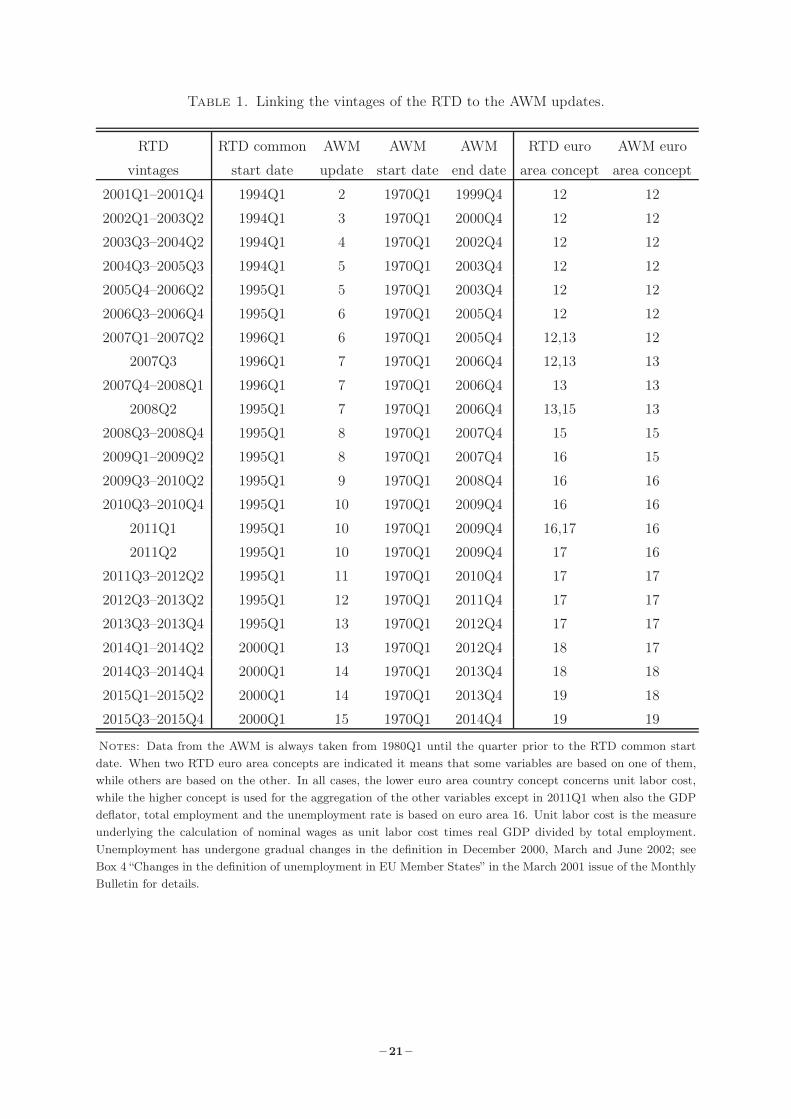
Table 1. Linking the vintages of the RTD to the AWM updates.

RTD RTD common AWM AWM AWM RTD euro AWM euro

vintages start date update start date end date area concept area concept

2001Q1–2001Q4 1994Q1 2 1970Q1 1999Q4 12 12

2002Q1–2003Q2 1994Q1 3 1970Q1 2000Q4 12 12

2003Q3–2004Q2 1994Q1 4 1970Q1 2002Q4 12 12

2004Q3–2005Q3 1994Q1 5 1970Q1 2003Q4 12 12

2005Q4–2006Q2 1995Q1 5 1970Q1 2003Q4 12 12

2006Q3–2006Q4 1995Q1 6 1970Q1 2005Q4 12 12

2007Q1–2007Q2 1996Q1 6 1970Q1 2005Q4 12,13 12

2007Q3 1996Q1 7 1970Q1 2006Q4 12,13 13

2007Q4–2008Q1 1996Q1 7 1970Q1 2006Q4 13 13

2008Q2 1995Q1 7 1970Q1 2006Q4 13,15 13

2008Q3–2008Q4 1995Q1 8 1970Q1 2007Q4 15 15

2009Q1–2009Q2 1995Q1 8 1970Q1 2007Q4 16 15

2009Q3–2010Q2 1995Q1 9 1970Q1 2008Q4 16 16

2010Q3–2010Q4 1995Q1 10 1970Q1 2009Q4 16 16

2011Q1 1995Q1 10 1970Q1 2009Q4 16,17 16

2011Q2 1995Q1 10 1970Q1 2009Q4 17 16

2011Q3–2012Q2 1995Q1 11 1970Q1 2010Q4 17 17

2012Q3–2013Q2 1995Q1 12 1970Q1 2011Q4 17 17

2013Q3–2013Q4 1995Q1 13 1970Q1 2012Q4 17 17

2014Q1–2014Q2 2000Q1 13 1970Q1 2012Q4 18 17

2014Q3–2014Q4 2000Q1 14 1970Q1 2013Q4 18 18

2015Q1–2015Q2 2000Q1 14 1970Q1 2013Q4 19 18

2015Q3–2015Q4 2000Q1 15 1970Q1 2014Q4 19 19

Notes: Data from the AWM is always taken from 1980Q1 until the quarter prior to the RTD common startdate. When two RTD euro area concepts are indicated it means that some variables are based on one of them,while others are based on the other. In all cases, the lower euro area country concept concerns unit labor cost,while the higher concept is used for the aggregation of the other variables except in 2011Q1 when also the GDPdeflator, total employment and the unemployment rate is based on euro area 16. Unit labor cost is the measureunderlying the calculation of nominal wages as unit labor cost times real GDP divided by total employment.Unemployment has undergone gradual changes in the definition in December 2000, March and June 2002; seeBox 4 “Changes in the definition of unemployment in EU Member States” in the March 2001 issue of the MonthlyBulletin for details.

– 21 –

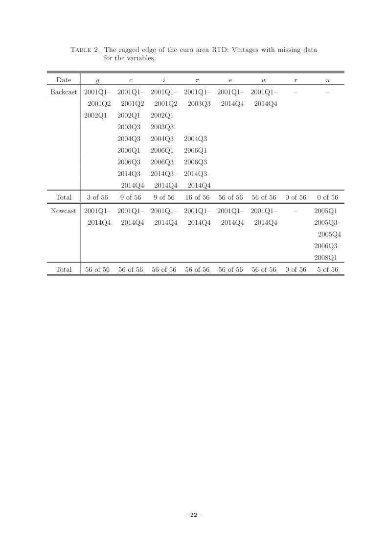
Table 2. The ragged edge of the euro area RTD: Vintages with missing datafor the variables.

Date y c i π e w r u

Backcast 2001Q1– 2001Q1– 2001Q1– 2001Q1– 2001Q1– 2001Q1– – –

2001Q2 2001Q2 2001Q2 2003Q3 2014Q4 2014Q4

2002Q1 2002Q1 2002Q1

2003Q3 2003Q3

2004Q3 2004Q3 2004Q3

2006Q1 2006Q1 2006Q1

2006Q3 2006Q3 2006Q3

2014Q3– 2014Q3– 2014Q3–

2014Q4 2014Q4 2014Q4

Total 3 of 56 9 of 56 9 of 56 16 of 56 56 of 56 56 of 56 0 of 56 0 of 56

Nowcast 2001Q1– 2001Q1– 2001Q1– 2001Q1– 2001Q1– 2001Q1– – 2005Q1

2014Q4 2014Q4 2014Q4 2014Q4 2014Q4 2014Q4 2005Q3–

2005Q4

2006Q3

2008Q1

Total 56 of 56 56 of 56 56 of 56 56 of 56 56 of 56 56 of 56 0 of 56 5 of 56

– 22 –

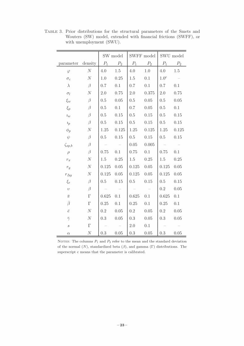
Table 3. Prior distributions for the structural parameters of the Smets andWouters (SW) model, extended with financial frictions (SWFF), orwith unemployment (SWU).

SW model SWFF model SWU model

parameter density P1 P2 P1 P2 P1 P2

ϕ N 4.0 1.5 4.0 1.0 4.0 1.5

σc N 1.0 0.25 1.5 0.1 1.0c –

λ β 0.7 0.1 0.7 0.1 0.7 0.1

σl N 2.0 0.75 2.0 0.375 2.0 0.75

ξw β 0.5 0.05 0.5 0.05 0.5 0.05

ξp β 0.5 0.1 0.7 0.05 0.5 0.1

ıw β 0.5 0.15 0.5 0.15 0.5 0.15

ıp β 0.5 0.15 0.5 0.15 0.5 0.15

φp N 1.25 0.125 1.25 0.125 1.25 0.125

ψ β 0.5 0.15 0.5 0.15 0.5 0.15

ζsp,b β – – 0.05 0.005 – –

ρ β 0.75 0.1 0.75 0.1 0.75 0.1

rπ N 1.5 0.25 1.5 0.25 1.5 0.25

ry N 0.125 0.05 0.125 0.05 0.125 0.05

r∆y N 0.125 0.05 0.125 0.05 0.125 0.05

ξe β 0.5 0.15 0.5 0.15 0.5 0.15

υ β – – – – 0.2 0.05

π Γ 0.625 0.1 0.625 0.1 0.625 0.1

β Γ 0.25 0.1 0.25 0.1 0.25 0.1

e N 0.2 0.05 0.2 0.05 0.2 0.05

γ N 0.3 0.05 0.3 0.05 0.3 0.05

s Γ – – 2.0 0.1 – –

α N 0.3 0.05 0.3 0.05 0.3 0.05

Notes: The columns P1 and P2 refer to the mean and the standard deviationof the normal (N), standardized beta (β), and gamma (Γ) distributions. Thesuperscript c means that the parameter is calibrated.

– 23 –

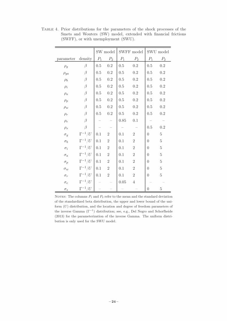
Table 4. Prior distributions for the parameters of the shock processes of theSmets and Wouters (SW) model, extended with financial frictions(SWFF), or with unemployment (SWU).

SW model SWFF model SWU model

parameter density P1 P2 P1 P2 P1 P2

ρg β 0.5 0.2 0.5 0.2 0.5 0.2

ρga β 0.5 0.2 0.5 0.2 0.5 0.2

ρb β 0.5 0.2 0.5 0.2 0.5 0.2

ρi β 0.5 0.2 0.5 0.2 0.5 0.2

ρa β 0.5 0.2 0.5 0.2 0.5 0.2

ρp β 0.5 0.2 0.5 0.2 0.5 0.2

ρw β 0.5 0.2 0.5 0.2 0.5 0.2

ρr β 0.5 0.2 0.5 0.2 0.5 0.2

ρe β – – 0.85 0.1 – –

ρs β – – – – 0.5 0.2

σg Γ−1/U 0.1 2 0.1 2 0 5

σb Γ−1/U 0.1 2 0.1 2 0 5

σi Γ−1/U 0.1 2 0.1 2 0 5

σa Γ−1/U 0.1 2 0.1 2 0 5

σp Γ−1/U 0.1 2 0.1 2 0 5

σw Γ−1/U 0.1 2 0.1 2 0 5

σr Γ−1/U 0.1 2 0.1 2 0 5

σe Γ−1/U – – 0.05 4 – –

σs Γ−1/U – – – – 0 5

Notes: The columns P1 and P2 refer to the mean and the standard deviationof the standardized beta distribution, the upper and lower bound of the uni-form (U) distribution, and the location and degree of freedom parameters ofthe inverse Gamma (Γ−1) distribution; see, e.g., Del Negro and Schorfheide(2013) for the parameterization of the inverse Gamma. The uniform distri-bution is only used for the SWU model.

– 24 –

Table 5. Mean errors based on predictive mean as point forecast for the sample2001Q1–2014Q4.

∆y π

h SW SWFF SWU SW SWFF SWU

-1 0.045 −0.337 −0.218 0.154 0.227 0.136

0 −0.168 −0.388 −0.279 0.067 0.228 0.039

1 −0.382 −0.595 −0.439 0.028 0.278 0.004

2 −0.472 −0.655 −0.490 −0.018 0.284 −0.040

3 −0.502 −0.666 −0.486 −0.064 0.270 −0.084

4 −0.488 −0.650 −0.443 −0.113 0.241 −0.132

5 −0.467 −0.637 −0.400 −0.155 0.211 −0.172

6 −0.440 −0.622 −0.358 −0.186 0.185 −0.202

7 −0.411 −0.607 −0.318 −0.215 0.155 −0.231

8 −0.380 −0.587 −0.279 −0.238 0.129 −0.252

– 25 –

Table 6. Point forecasts of real GDP growth of the SWU model for the 2008Q4and 2009Q1 vintages.

Forecast horizon

Vintage 0 1 2 3 4 5 6 7 8

2008Q4 0.144 0.276 0.350 0.385 0.399 0.400 0.395 0.389 0.382

2009Q1 0.214 0.596 0.710 0.721 0.687 0.634 0.576 0.521 0.472

Point forecasts from the 2009Q1 vintage subject to input change

Source 0 1 2 3 4 5 6 7 8

Parameters 0.289 0.665 0.764 0.766 0.724 0.665 0.602 0.543 0.491

Revisions −0.001 0.394 0.401 0.364 0.331 0.310 0.301 0.299 0.303

New data 0.349 0.406 0.421 0.417 0.405 0.391 0.378 0.367 0.358

Old data 0.240 0.308 0.342 0.358 0.362 0.360 0.357 0.354 0.351

Actuals −2.529 −0.110 0.421 0.199 0.388 0.953 0.382 0.268 0.751

Notes: The three cases for changes to the construction of the 2009Q1 vintage point forecasts aredefined as follows: Parameters refers to changing the posterior parameter draws from the 2009Q1vintage to the 2008Q4 vintage draws; Revisions means that all the historical data from the 2008Q4vintage are used instead of the data for the same time periods from the 2009Q1 vintage, whilethe latest data points from the 2009Q1 vintage are still taken into account; New data refers tothe case when the latest data points for each variable from the 2009Q1 vintage are excluded fromthe dataset and where the data prior to these dates are included; while Old data means that onlydata from the 2008Q4 vintage are used and where the latest data points from the 2009Q1 vintageare therefore treated as unobserved.

– 26 –

Table 7. Differences in log predictive score between the MC estimator and thenormal approximation for the sample 2001Q1–2014Q4.

∆y π ∆y & π

h SW SWFF SWU SW SWFF SWU SW SWFF SWU

-1 0.012 0.015 0.008 0.060 −0.042 0.025 0.030 −0.024 0.055

0 0.292 0.195 0.617 0.094 0.028 0.073 0.375 0.162 0.688

1 0.498 0.444 0.485 0.358 0.153 0.265 0.885 0.500 0.852

2 0.474 0.442 0.444 0.486 0.329 0.320 1.004 0.668 0.900

3 0.502 0.458 0.474 0.473 0.414 0.297 1.002 0.790 0.890

4 0.529 0.481 0.496 0.444 0.508 0.253 0.974 0.899 0.846

5 0.497 0.471 0.467 0.394 0.559 0.218 0.908 1.005 0.804

6 0.513 0.489 0.468 0.349 0.597 0.187 0.906 1.080 0.792

7 0.513 0.493 0.472 0.272 0.644 0.122 0.827 1.151 0.719

8 0.477 0.512 0.451 0.227 0.664 0.082 0.752 1.213 0.669

– 27 –

Figure 1. Euro area RTD vintages 2001Q1–2015Q4 extended back in time usingAWM database annual vintages.

Real GDP, ∆yt Private consumption, ∆ct Total investment, ∆it

GDP deflator, πt Total employment, ∆et Real wages, ∆wt

Nominal interest rate, rt Unemployment, ut

RTD 2001

RTD 2003

RTD 2005

RTD 2007

RTD 2009

RTD 2011

RTD 2013

RTD 20151980 1980

198019801980

198019801980

1990 1990

199019901990

199019901990

2000 2000

200020002000

200020002000

2010 2010

201020102010

201020102010

15 12

1010

8

65

4

3

2

2

2

1

1

11

0.5

0

00

0

000

-0.5-1

-1-1 -2

-2-2-3

-4-6

– 28 –

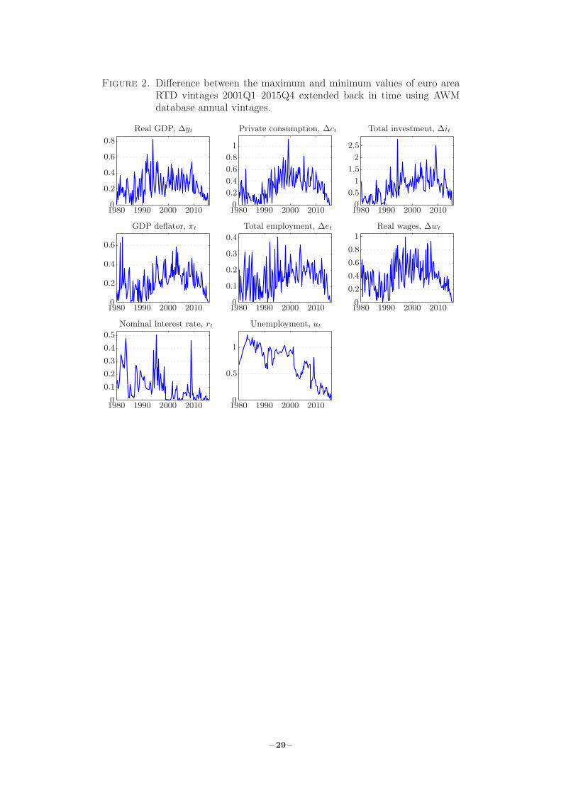
Figure 2. Difference between the maximum and minimum values of euro areaRTD vintages 2001Q1–2015Q4 extended back in time using AWMdatabase annual vintages.

Real GDP, ∆yt Private consumption, ∆ct Total investment, ∆it

GDP deflator, πt Total employment, ∆et Real wages, ∆wt

Nominal interest rate, rt Unemployment, ut

1980 1980

198019801980

198019801980

1990 1990

199019901990

199019901990

2000 2000

200020002000

200020002000

2010 2010

201020102010

201020102010

2.52

1.5

1

1

1

1

0.8

0.8

0.8

0.6

0.6

0.60.6

0.5

0.5

0.5

0.4

0.4

0.4

0.4

0.40.4

0.3

0.3

0.2

0.2

0.2

0.2

0.20.2

0.1

0.1

0 0

000

000

– 29 –

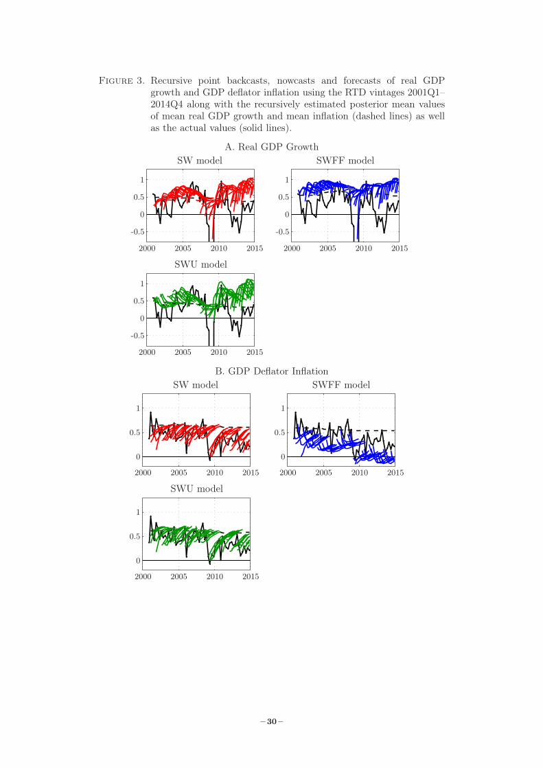
Figure 3. Recursive point backcasts, nowcasts and forecasts of real GDPgrowth and GDP deflator inflation using the RTD vintages 2001Q1–2014Q4 along with the recursively estimated posterior mean valuesof mean real GDP growth and mean inflation (dashed lines) as wellas the actual values (solid lines).

A. Real GDP GrowthSW model SWFF model

SWU model

2000

20002000

2005

20052005

2010

20102010

2015

20152015

1

11

0.5

0.50.5

0

00

-0.5

-0.5-0.5

B. GDP Deflator InflationSW model SWFF model

SWU model

2000

20002000

2005

20052005

2010

20102010

2015

20152015

1

11

0.5

0.50.5

0

00

– 30 –

Figure 4. Log predictive scores based on the MC estimator of the predictivelikelihood for real GDP growth and inflation based on backcasts,nowcasts, and one-to eight-quarter-head forecasts over the vintages2001Q1–2014Q4.

GDP deflator inflationReal GDP growth

Joint

20

10

8

8 8

6

6 6

4

4 4

2

2 2

0

0

0

0

0

0

-10

-20

-20

-40

-50

-60

-80

-100

SW modelSWFF modelSWU model

Notes: Forecast horizons are displayed on the horizontal axis with h = −1 being the backcast horizon and h = 0

the nowcast horizon.

– 31 –

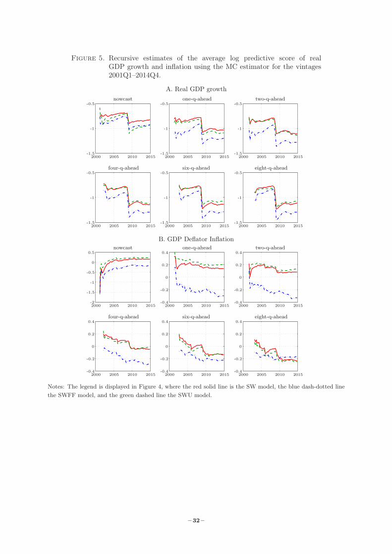
Figure 5. Recursive estimates of the average log predictive score of realGDP growth and inflation using the MC estimator for the vintages2001Q1–2014Q4.

A. Real GDP growthnowcast one-q-ahead two-q-ahead

four-q-ahead six-q-ahead eight-q-ahead

200020002000

200020002000

200520052005

200520052005

201020102010

201020102010

201520152015

201520152015

-0.5-0.5-0.5

-0.5-0.5-0.5

-1-1-1

-1-1-1

-1.5-1.5-1.5

-1.5-1.5-1.5

B. GDP Deflator Inflationnowcast one-q-ahead two-q-ahead

four-q-ahead six-q-ahead eight-q-ahead

200020002000

200020002000

200520052005

200520052005

201020102010

201020102010

201520152015

201520152015

0.5

0.40.40.4

0.40.4

0.20.20.2

0.20.2

000

00

0

-0.2-0.2-0.2

-0.2-0.2

-0.4-0.4-0.4

-0.4-0.4

-0.5

-1

-1.5

-2

Notes: The legend is displayed in Figure 4, where the red solid line is the SW model, the blue dash-dotted linethe SWFF model, and the green dashed line the SWU model.

– 32 –

Figure 6. Recursive estimates of the average log predictive score of realGDP growth and inflation using the MC estimator for the vintages2008Q4–2014Q4.

A. Real GDP growthnowcast one-q-ahead two-q-ahead

four-q-ahead six-q-ahead eight-q-ahead

200820082008

200820082008

201020102010

201020102010

201220122012

201220122012

201420142014

201420142014

-0.7-0.7-0.7

-0.7

-0.9-0.9-0.9

-0.9

-1.1-1.1-1.1

-1.1

-1.3-1.3-1.3

-1.3

00

-0.8-0.8-0.8

-0.8

-1-1-1

-1

-1.2-1.2-1.2

-1.2

-2-2

-4-4

-6

-6 -8

-8 -10

B. GDP Deflator Inflationnowcast one-q-ahead two-q-ahead

four-q-ahead six-q-ahead eight-q-ahead

200820082008

200820082008

201020102010

201020102010

201220122012

201220122012

201420142014

201420142014

-0.5-0.5-0.5

-0.5-0.5

0.40.3

0.20.1

000

00

0-0.1-0.2

-1-1-1

-1-1

Notes: See the notes to Figure 4.

– 33 –

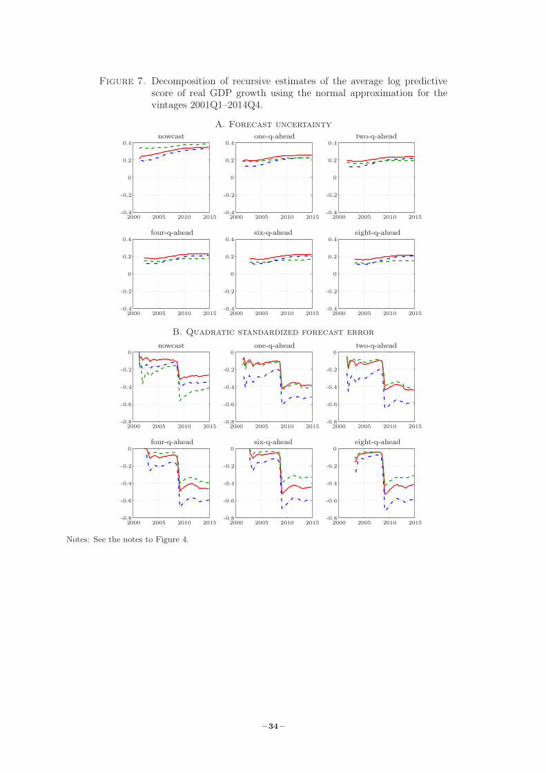
Figure 7. Decomposition of recursive estimates of the average log predictivescore of real GDP growth using the normal approximation for thevintages 2001Q1–2014Q4.

A. Forecast uncertaintynowcast one-q-ahead two-q-ahead

four-q-ahead six-q-ahead eight-q-ahead

200020002000

200020002000

200520052005

200520052005

201020102010

201020102010

201520152015

201520152015

0.40.40.4

0.40.40.4

0.20.20.2

0.20.20.2

000

000

-0.2-0.2-0.2

-0.2-0.2-0.2

-0.4-0.4-0.4

-0.4-0.4-0.4

B. Quadratic standardized forecast errornowcast one-q-ahead two-q-ahead

four-q-ahead six-q-ahead eight-q-ahead

200020002000

200020002000

200520052005

200520052005

201020102010

201020102010

201520152015

201520152015

000

000

-0.2-0.2-0.2

-0.2-0.2-0.2

-0.4-0.4-0.4

-0.4-0.4-0.4

-0.6-0.6-0.6

-0.6-0.6-0.6

-0.8-0.8-0.8

-0.8-0.8-0.8

Notes: See the notes to Figure 4.

– 34 –

Figure 8. Decomposition of recursive estimates of the average log predictivescore of inflation using the normal approximation for the vintages2001Q1–2014Q4.

A. Forecast uncertaintynowcast one-q-ahead two-q-ahead

four-q-ahead six-q-ahead eight-q-ahead

200020002000

200020002000

200520052005

200520052005

201020102010

201020102010

201520152015

201520152015

3

2.5

2

1.5

1.41.41.4

1.41.4

1.21.21.2

1.21.2

111

11

1

0.80.80.8

0.80.8

0.60.60.6

0.60.6

B. Quadratic standardized forecast errornowcast one-q-ahead two-q-ahead

four-q-ahead six-q-ahead eight-q-ahead

200020002000

200020002000

200520052005

200520052005

201020102010

201020102010

201520152015

201520152015

000

000

-0.1-0.1-0.1

-0.1-0.1

-0.2-0.2-0.2

-0.2-0.2

-0.3-0.3-0.3

-0.3-0.3

-0.4-0.4-0.4

-0.4-0.4

-0.5-0.5-0.5

-0.5-0.5

-0.5

-0.6-0.6-0.6

-0.6-0.6

-1

-1.5

-2

Notes: See the notes to Figure 4.

– 35 –

References

Adolfson, M., Laséen, S., Lindé, J., and Villani, M. (2007a), “Bayesian Estimation of an Open

Economy DSGE Model with Incomplete Pass-Through,” Journal of International Economics,

72(2), 481–511.

Adolfson, M., Lindé, J., and Villani, M. (2007b), “Forecasting Performance of an Open Economy

DSGE Model,” Econometric Reviews, 26(2), 289–328.

Amisano, G. and Geweke, J. (2017), “Prediction Using Several Macroeconomic Models,” Review

of Economics and Statistics, 99(5), 912–925.

An, S. and Schorfheide, F. (2007), “Bayesian Analysis of DSGE Models,” Econometric Reviews,

26(2), 113–172.

Bernanke, B. S., Gertler, M., and Gilchrist, S. (1999), “The Financial Accelerator in a Quanti-

tative Business Cycle Framework,” in J. B. Taylor and M. Woodford (Editors), Handbook of

Macroeconomics, volume 1C, 1341–1393, North Holland, Amsterdam.

Buch, C. M. and Holtemöller, O. (2014), “Do we need New Modelling Approaches in Macroe-

conomics?” in Financial Cycles and the Real Economy, chapter 3, 36–58, Edward Elgar

Publishing.

Caballero, R. J. (2010), “Macroeconomics after the Crisis: Time to Deal with the Pretense-of-

Knowledge Syndrome,” Journal of Economic Perspectives, 24(4), 85–102.

Chari, V. V., Kehoe, P. J., and McGrattan, E. R. (2009), “New Keynesian Models: Not Yet

Useful for policy Analysis,” American Economic Journal: Macroeconomics, 1(1), 242–266.

Christiano, L. J., Motto, R., and Rostagno, M. (2003), “The Great Depression and the Friedman-

Schwartz Hypothesis,” Journal of Money, Credit, and Banking, 35(6), 1119–1197.

Christiano, L. J., Motto, R., and Rostagno, M. (2008), “Shocks, Structures or Monetary Policies?

The Euro Area and US After 2001,” Journal of Economic Dynamics and Control, 32(8), 2476–

2506.

Christiano, L. J., Trabandt, M., and Walentin, K. (2011), “Introducing Financial Frictions and

Unemployment into a Small Open Economy Model,” Journal of Economic Dynamics and

Control, 35(12), 1999–2041.

Coenen, G., Levin, A., and Wieland, V. (2005), “Data Uncertainty and the Role of Money as

Information Variable for Monetary Policy,” European Economic Review, 49(4), 975–1006.

Coenen, G. and Warne, A. (2014), “Risks to Price Stability, the Zero Lower Bound and Forward

Guidance: A Real-Time Assessment,” International Journal of Central Banking, 10(2), 7–54.

Conflitti, C., De Mol, C., and Giannone, D. (2015), “Optimal Combination of Survey Forecasts,”

International Journal of Forecasting, 31(4), 1096–1103.

Croushore, D. (2011), “Frontiers of Real-Time Data Analysis,” Journal of Economic Literature,

49(1), 72–110.

Croushore, D. and Stark, T. (2001), “A Real-Time Data Set for Macroeconomists,” Journal of

Econometrics, 105(1), 111–130.

– 36 –

Darracq Paries, M., Kok Sørensen, C., and Rodriguez-Palenzuela, D. (2011), “Macroeconomic

Propagation under Different Regulatory Regimes: Evidence from an Estimated DSGE Model

for the Euro Area,” International Journal of Central Banking, 7(4), 49–113.

De Graeve, F. (2008), “The External Finance Premium and the Macroeconomy: US Post-WWII

Evidence,” Journal of Economic Dynamics and Control, 32(11), 3415–3440.

Del Negro, M., Giannoni, M. P., and Schorfheide, F. (2015), “Inflation in the Great Recession

and New Keynesian Models,” American Economic Journal: Macroeconomics, 7(1), 168–196.

Del Negro, M. and Schorfheide, F. (2013), “DSGE Model-Based Forecasting,” in G. Elliott

and A. Timmermann (Editors), Handbook of Economic Forecasting, volume 2, 57–140, North

Holland, Amsterdam.

European Commission (2016), “Labour Market and Wage Developments in Europe Annual Re-

view,” European Commission.

Fagan, G., Henry, J., and Mestre, R. (2005), “An Area-Wide Model for the Euro Area,” Economic

Modelling, 22(1), 39–59.

Fisher, J. D. M. (2015), “On the Structural Interpretation of the Smets-Wouters “Risk Premium”

Shock,” Journal of Money, Credit and Banking, 47(2–3), 511–516.

Galí, J. (2011), “The Return Of The Wage Phillips Curve,” Journal of the European Economic

Association, 9(3), 436–461.

Galí, J., Smets, F., and Wouters, R. (2012), “Unemployment in an Estimated New Keynesian

Model,” in D. Acemoglu and M. Woodford (Editors), NBER Macroeconomics Annual 2011,

329–360, University of Chicago Press.

Geweke, J. and Amisano, G. (2011), “Optimal Prediction Pools,” Journal of Econometrics,

164(1), 130–141.

Geweke, J. and Amisano, G. (2014), “Analysis of Variance for Bayesian Inference,” Econometric

Reviews, 33(1–4), 270–288.

Giannone, D., Henry, J., Lalik, M., and Modugno, M. (2012), “An Area-Wide Real-Time Data-

base for the Euro Area,” Review of Economics and Statistics, 94(4), 1000–1013.

Gneiting, T. and Raftery, A. E. (2007), “Strictly Proper Scoring Rules, Prediction, and Estima-

tion,” Journal of the American Statistical Association, 102, 359–378.

Hall, R. E. (2010), “Why Does the Economy Fall to Pieces after a Financial Crisis?” Journal of

Economic Perspectives, 24(4), 45–66.

Iacoviello, M. (2005), “House Prices, Borrowing Constraints, and Monetary Policy in the Busi-

ness Cycle,” American Economic Review, 95(3), 739–764.

Iskrev, N. (2010), “Local Identification in DSGE Models,” Journal of Monetary Economic, 57(2),

189–202.

Kimball, M. S. (1995), “The Quantitative Analytics of the Basic Nonmonetarist Model,” Journal

of Money, Credit, and Banking, 27(4), 1241–77.

– 37 –

Kolasa, M. and Rubaszek, M. (2015), “Forecasting using DSGE Models with Financial Frictions,”

International Journal of Forecasting, 31(1), 1–19.

Kolasa, M., Rubaszek, M., and Skrzypczyński, P. (2012), “Putting the New Keynesian DSGE

Model to the Real-Time Forecasting Test,” Journal of Money, Credit, and Banking, 44(7),

1301–1324.

Levine, P., McAdam, P., and Pearlman, J. (2008), “Quantifying and Sustaining Welfare Gains

from Monetary Commitment,” Journal of Monetary Economics, 55(7), 1253–1276.

Lindé, J., Smets, F., and Wouters, R. (2016), “Challenges for Central Banks’ Macro Models,”

in J. B. Taylor and H. Uhlig (Editors), Handbook of Macroeconomics, volume 2B, 2185–2262,

North Holland, Amsterdam.

Lombardo, G. and McAdam, P. (2012), “Financial Market Frictions in a Model of the Euro

Area,” Economic Modelling, 29(6), 2460–2485.

McAdam, P. and Warne, A. (2018), “Euro Area Real-Time Density Forecasting with Financial

or Labor Market Frictions,” Forthcoming in the ECB Working Paper Series. Available for

download at: http://www.texlips.net/awarne/researchpapers.html.

Ohanian, L. (2010), “The Economic Crisis from a Neoclassical Perspective,” Journal of Economic

Perspectives, 24(4), 45–66.

Pirschel, I. (2016), “Forecasting Euro Area Recessions in Real-Time,” Kiel Working Paper, No.

2020.

Smets, F., Warne, A., and Wouters, R. (2014), “Professional Forecasters and Real-Time Fore-

casting with a DSGE Model,” International Journal of Forecasting, 30(4), 981–995.

Smets, F. and Wouters, R. (2003), “An Estimated Stochastic Dynamic General Equilibrium

Model for the Euro Area,” Journal of the European Economic Association, 1(5), 1123–1175.

Smets, F. and Wouters, R. (2005), “Comparing Shocks and Frictions in U.S. and Euro Area

Business Cycles: A Bayesian DSGE Approach,” Journal of Applied Econometrics, 20(2), 161–

183.

Smets, F. and Wouters, R. (2007), “Shocks and Frictions in US Business Cycles: A Bayesian

DSGE Approach,” American Economic Review, 97(3), 586–606.

Tierney, L. (1994), “Markov Chains for Exploring Posterior Distributions,” The Annals of Sta-

tistics, 22(4), 1701–1728, with discussion, p. 1728–1762.

Wallis, K. F. (1986), “Forecasting with an Econometric Model: The Ragged Edge Problem,”

Journal of Forecasting, 5(1), 1–13.

Warne, A. (2017), “YADA Manual — Computational Details,” Manuscript, European Central

Bank. Available with the YADA distribution.

Warne, A., Coenen, G., and Christoffel, K. (2017), “Marginalized Predictive Likelihood Com-

parisons of Linear Gaussian State-Space Models with Applications to DSGE, DSGE-VAR and

VAR Models,” Journal of Applied Econometrics, 32(1), 103–119.

– 38 –

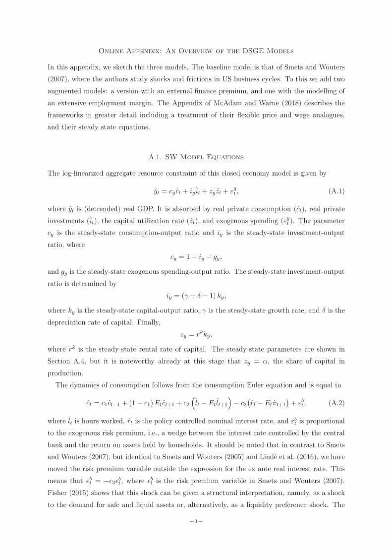
Online Appendix: An Overview of the DSGE Models

In this appendix, we sketch the three models. The baseline model is that of Smets and Wouters

(2007), where the authors study shocks and frictions in US business cycles. To this we add two

augmented models: a version with an external finance premium, and one with the modelling of

an extensive employment margin. The Appendix of McAdam and Warne (2018) describes the

frameworks in greater detail including a treatment of their flexible price and wage analogues,

and their steady state equations.

A.1. SW Model Equations

The log-linearized aggregate resource constraint of this closed economy model is given by

yt = cy ct + iy it + zyzt + εgt , (A.1)

where yt is (detrended) real GDP. It is absorbed by real private consumption (ct), real private

investments (it), the capital utilization rate (zt), and exogenous spending (εgt ). The parameter

cy is the steady-state consumption-output ratio and iy is the steady-state investment-output

ratio, where

cy = 1 − iy − gy,

and gy is the steady-state exogenous spending-output ratio. The steady-state investment-output

ratio is determined by

iy = (γ + δ − 1) ky,

where ky is the steady-state capital-output ratio, γ is the steady-state growth rate, and δ is the

depreciation rate of capital. Finally,

zy = rkky,

where rk is the steady-state rental rate of capital. The steady-state parameters are shown in

Section A.4, but it is noteworthy already at this stage that zy = α, the share of capital in

production.

The dynamics of consumption follows from the consumption Euler equation and is equal to

ct = c1ct−1 + (1 − c1)Etct+1 + c2

(lt − Et lt+1

)− c3

(rt − Etπt+1

)+ εbt , (A.2)

where lt is hours worked, rt is the policy controlled nominal interest rate, and εbt is proportional

to the exogenous risk premium, i.e., a wedge between the interest rate controlled by the central

bank and the return on assets held by households. It should be noted that in contrast to Smets

and Wouters (2007), but identical to Smets and Wouters (2005) and Lindé et al. (2016), we have

moved the risk premium variable outside the expression for the ex ante real interest rate. This

means that εbt = −c3εbt , where εbt is the risk premium variable in Smets and Wouters (2007).

Fisher (2015) shows that this shock can be given a structural interpretation, namely, as a shock

to the demand for safe and liquid assets or, alternatively, as a liquidity preference shock. The

– 1 –

parameters of the consumption Euler equation are:

c1 =λ/γ

1 + (λ/γ), c2 =

(σc − 1) (whl/c)σc (1 + (λ/γ))

, c3 =1 − (λ/γ)

σc (1 + (λ/γ)),

where λ measures external habit formation, σc is the inverse of the elasticity of intertemporal

substitution for constant labor, while whl/c is the steady-state hourly real wage bill to consump-

tion ratio. If σc = 1 (log-utility) and λ = 0 (no external habit) then the above equation reduces

to the familiar purely forward looking consumption Euler equation.

The log-linearized investment Euler equation is given by

it = i1 it−1 + (1 − i1)Etit+1 + i2qt + εit, (A.3)

where qt is the real value of the existing capital stock, while εit is an exogenous investment-specific

technology variable. The parameters of (A.3) are given by

i1 =1

1 + βγ1−σc, i2 =

1(1 + βγ1−σc) γ2ϕ

,

where β is the discount factor used by households, and ϕ is the steady-state elasticity of the

capital adjustment cost function.

The dynamic equation for the value of the capital stock is

qt = q1Etqt+1 + (1 − q1)Etrkt+1 −

(rt − Etπt+1

)+ c−1

3 εbt , (A.4)

where rkt is the rental rate of capital. The parameter q1 is here given by

q1 = βγ−σc(1 − δ) =1 − δ

rk + 1 − δ.

Turning to the supply-side of the economy, the log-linearized aggregate production function

can be expressed as

yt = φp

[αks

t + (1 − α) lt + εat

], (A.5)

where kst is capital services used in production, and εat an exogenous total factor productivity

variable. As mentioned above, the parameter α reflects the share of capital in production, while

φp is equal to one plus the steady-state share of fixed costs in production.

The capital services variable is used to reflect that newly installed capital only becomes

effective with a one period lag. This means that

kst = kt−1 + zt, (A.6)

where kt is the installed capital. The degree of capital utilization is determined from cost

minimization of the households that provide capital services and is therefore a positive function

of the rental rate of capital. Specifically,

zt = z1rkt , (A.7)

– 2 –

where z1 =1 − ψ

ψand ψ is a positive function of the elasticity of the capital adjustment cost

function and normalized to lie between 0 and 1. The larger ψ is the costlier it is to change

the utilization of capital. The log-linearized equation that specifies the development of installed

capital is

kt = k1kt−1 + (1 − k1) it + k2εit. (A.8)

where k1 =1 − δ

γand k2 = (γ + δ − 1)

(1 + βγ1−σc

)γϕ.

From the monopolistically competitive goods market, the price markup (µpt ) is equal to minus

the real marginal cost (µct) under cost minimization by firms. That is,

µpt = α

(ks

t − lt

)− wt + εat , (A.9)

where the real wage is given by wt. Similarly, the real marginal cost is

µct = αrk

t + (1 − α) wt − εat , (A.10)

where (A.10) is obtained by substituting for the optimally determined capital-labor ratio in

equation (A.12).

Due to price stickiness, and partial indexation to lagged inflation of those prices that cannot

be re-optimized, prices adjust only sluggishly to their desired markups. Profit maximization by

price-setting firms yields the log-linearized price Phillips curve,

πt = π1πt−1 + π2Etπt+1 − π3µpt + εpt

= π1πt−1 + π2Etπt+1 + π3µct + εpt ,

(A.11)

where εpt is an exogenous price markup process. The parameters of the Phillips curve are given

by

π1 =ıp

1 + βγ1−σc ıp, π2 =

βγ1−σc

1 + βγ1−σc ıp, π3 =

(1 − ξp)(1 − βγ1−σcξp

)(1 + βγ1−σc ıp) ξp ((φp − 1)εp + 1)

.

The degree of indexation to past inflation is determined by the parameter ıp, ξp measures the

degree of price stickiness such that 1− ξp is the probability that a firm can re-optimize its price,

and εp is the curvature of the Kimball (1995) goods market aggregator.

Cost minimization of firms also implies that the rental rate of capital is related to the capital-

labor ratio and the real wage according to.

rkt = −

(ks

t − lt

)+ wt. (A.12)

In the monopolistically competitive labor market the wage markup is equal to the difference

between the real wage and the marginal rate of substitution between labor and consumption

µwt = wt −

(σl lt +

11 − (λ/γ)

[ct − λ

γct−1

]), (A.13)

where σl is the elasticity of the labor input with respect to real wages.

– 3 –

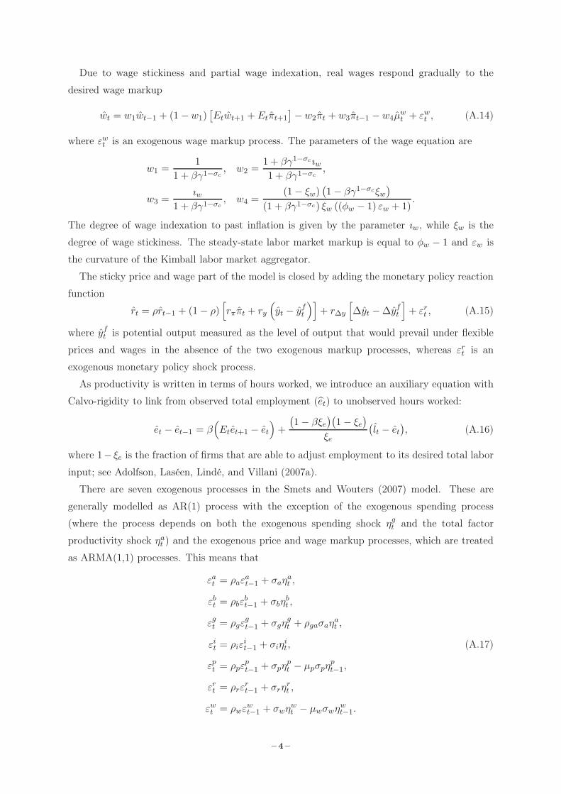
Due to wage stickiness and partial wage indexation, real wages respond gradually to the

desired wage markup

wt = w1wt−1 + (1 −w1)[Etwt+1 + Etπt+1

] −w2πt + w3πt−1 − w4µwt + εwt , (A.14)

where εwt is an exogenous wage markup process. The parameters of the wage equation are

w1 =1

1 + βγ1−σc, w2 =

1 + βγ1−σc ıw1 + βγ1−σc

,

w3 =ıw

1 + βγ1−σc, w4 =

(1 − ξw)(1 − βγ1−σcξw

)(1 + βγ1−σc) ξw ((φw − 1) εw + 1)

.

The degree of wage indexation to past inflation is given by the parameter ıw, while ξw is the

degree of wage stickiness. The steady-state labor market markup is equal to φw − 1 and εw is

the curvature of the Kimball labor market aggregator.

The sticky price and wage part of the model is closed by adding the monetary policy reaction

function

rt = ρrt−1 + (1 − ρ)[rππt + ry

(yt − yf

t

)]+ r∆y

[∆yt − ∆yf

t

]+ εrt , (A.15)

where yft is potential output measured as the level of output that would prevail under flexible

prices and wages in the absence of the two exogenous markup processes, whereas εrt is an

exogenous monetary policy shock process.

As productivity is written in terms of hours worked, we introduce an auxiliary equation with

Calvo-rigidity to link from observed total employment (et) to unobserved hours worked:

et − et−1 = β(Etet+1 − et

)+

(1 − βξe

)(1 − ξe

)ξe

(lt − et

), (A.16)

where 1− ξe is the fraction of firms that are able to adjust employment to its desired total labor

input; see Adolfson, Laséen, Lindé, and Villani (2007a).

There are seven exogenous processes in the Smets and Wouters (2007) model. These are

generally modelled as AR(1) process with the exception of the exogenous spending process

(where the process depends on both the exogenous spending shock ηgt and the total factor

productivity shock ηat ) and the exogenous price and wage markup processes, which are treated

as ARMA(1,1) processes. This means that

εat = ρaεat−1 + σaη

at ,

εbt = ρbεbt−1 + σbη

bt ,

εgt = ρgεgt−1 + σgη

gt + ρgaσaη

at ,

εit = ρiεit−1 + σiη

it,

εpt = ρpεpt−1 + σpη

pt − µpσpη

pt−1,

εrt = ρrεrt−1 + σrη

rt ,

εwt = ρwεwt−1 + σwη

wt − µwσwη

wt−1.

(A.17)

– 4 –

The shocks ηjt , j = {a, b, g, i, p, r, w}, are N(0, 1), where ηb

t is a preference shock (proportional

to a risk premium shock), ηit is an investment-specific technology shock, ηp

t is a price markup

shock, ηrt is a monetary policy or interest rate shock, and ηw

t is a wage markup shock.

A.2. The SWFF Model

Lombardo and McAdam (2012) and Del Negro and Schorfheide (2013) introduce financial fric-

tions into variants of the SW model based on the financial accelerator approach of Bernanke

et al. (1999); see also Christiano et al. (2003, 2008) and De Graeve (2008). This amounts to

replacing the value of the capital stock equation in (A.4) with

Etret+1 − rt = ζsp,b

(qt + kt − nt

) − c−13 εbt + εet , (A.18)

and

ret − πt =

(1 − q1

)rkt + q1qt − qt−1, (A.19)

where ret is the gross return on capital for entrepreneurs, nt is entrepreneurial equity (net worth),

and εet captures mean-preserving changes in the cross-sectional dispersion of ability across en-

trepreneurs, a spread shock. The parameter q1 is here given by

q1 =1 − δ

rk + 1 − δ,

where rk is generally not equal to β−1γσc + δ − 1 since the spread between gross returns on

capital for entrepreneurs and the nominal interest rate need not equal zero. The spread shock

is assumed to follows the AR(1) process

εet = ρeεet−1 + σeη

et . (A.20)

The parameters ζsp,b is the steady-state elasticity of the spread with respect to leverage. It may

be noted that if ζsp,b = σe = 0, then the financial frictions are shut down and equations (A.18)

and (A.19) yield the original value of the capital stock equation (A.4).

The log-linearized net worth of entrepreneurs equation is given by

nt = ζn,e

(ret − πt

) − ζn,r

(rt−1 − πt

)+ ζn,q

(qt−1 + kt−1

)+ ζn,nnt−1 − ζn,σω

ζsp,σω

εet−1, (A.21)

where ζn,e, ζn,r, ζn,q, ζn,n, and ζn,σω are the steady-state elasticities of net worth with respect to

the return on capital for entrepreneurs, the interest rate, the cost of capital, lagged net worth,

and the volatility of the spread shock. Furthermore, ζsp,σω is the steady-state elasticity of the

spread with respect to the spread shock. Expressions for these elasticities are given in McAdam

and Warne (2018, Section A.10).

A.3. The SWU Model

The Galí, Smets, and Wouters (2012, GSW) model is an extension of the standard SW model

which explicitly provides a mechanism for explaining unemployment. This is accomplished by

– 5 –

modelling the labor supply decisions on the extensive margin (whether to work or not) rather

than on the intensive margin (how many hours to work). As a consequence, the unemployment

rate is added as an observable variable, while labor supply shocks are admitted. This allows the

authors to overcome the lack of identification of wage markup and labor supply shocks raised

by Chari, Kehoe, and McGrattan (2009) in their critique of new Keynesian models. From a

technical perspective the GSW model is also based on the assumption of log-utility, i.e. the

parameter σc is assumed to be unity, but the equations presented below will instead be written

as if this is a free parameter and therefore treat σc as in McAdam and Warne (2018, Section A.1

and A.7).

Smets, Warne, and Wouters (2014) present a variant of the GSW model aimed for the euro

area and this version is presented below. The log-linearized aggregate resource constraint is

given by equation (A.1). The consumption Euler equation may be expressed as

λt = Etλt+1 +(rt − Etπt+1

) − c−13 εbt , (A.22)

where λt is the log-linearized marginal utility of consumption, given by

λt = − σc

1 − (λ/γ)

[ct − λ

γct−1

]+

(σc − 1)(whl/c)1 − (λ/γ)

lt, (A.23)

while εbt is the preference shock. Making use of (A.22) and (A.23), the consumption Euler

equation can be written in the more familiar form in equation (A.2), and where c3 is given by

the expressions below this equation. However, below we have use for the expression for λt.

Concerning the Phillips curve, it is similar to equation (A.11), but differs in the way that the

price markup shock enters the model:

πt = π1πt−1 + π2Etπt+1 − π3

(µp

t − µn,pt

). (A.24)

The expressions for πi below equation (A.11) hold and the natural price markup shock µn,pt =

100εpt . The average price markup and the real marginal cost variables are given by equation (A.9)

and (A.10), respectively. Relative to equation (A.11), the price markup shock εpt = π3100εpt .

Smets, Warne, and Wouters (2014) uses the shock εpt , while we wish to treat the price markup

shock symmetrically in the three models and therefore keep equation (A.11) such that our price

markup shock is given by εpt .23

In the GSW model, the wage Phillips curve in equation (A.14) is replaced with the following

expression for real wages

wt = w1wt−1 + (1 − w1)[Etwt+1 + Etπt+1

] − w2πt + w3πt−1 −w4

[µw

t − µn,wt

], (A.25)

23This has the advantage of separating the parameters describing the price markup shock process from theparameters of the price Phillips curve as π3 is no longer multiplied by the shock process. This separation ofparameters may be also useful when estimating the parameters of the model.

– 6 –

where µwt is the average wage markup and µn,w

t is the natural wage markup. Notice that the wi

parameters are given by the expressions below equation (A.14) for i = 1, 2, 3, while

w4 =

(1 − ξw

)(1 − βγ1−σcξw

)(1 + βγ1−σc

)ξw

(1 + εwσl

) .In addition, GSW and Smets, Warne, and Wouters (2014) let the curvature of the Kimball labor

market aggregator be given by εw =φw

φw − 1.

The average wage markup is defined as the difference between the real wage and the marginal

rate of substitution, which is a function of the adjusted smoothed trend in consumption, xt,

the marginal utility of consumption λt, total employment, et, and the labor supply shock. This

expression is equal to the elasticity of labor supply times the unemployment rate, i.e.

µwt = σlut

= wt −(xt − λt + εst + σlet

),

(A.26)

where unemployment is defined as labor supply minus total employment:

ut = lst − et. (A.27)

The labor supply shock is assumed to follow and AR(1) process such that

εst = ρsεst−1 + σsη

st . (A.28)

The natural wage markup shock is expressed as 100εwt and is, in addition, equal to the elasticity

of labor supply times the natural rate of unemployment. Accordingly,

µn,wt = 100εwt = σlu

nt . (A.29)

The natural rate of unemployment, unt , is defined as the unemployment rate that would prevail

in the absence of nominal wage rigidities, and is here proportional to the natural wage markup.

Finally, we here let the wage markup shock, εwt , be defined such that:

εwt = w4µn,wt = w4100εwt .

Hence, the wage markup shock εwt enters equation (A.25) suitably re-scaled and, apart from the

definition of the w4 parameter, the wage Phillips curve is identical to equation (A.14). This has

the advantage of allowing us to treat the wage markup shock as symmetrically as possible in the

three models.24

The adjusted smoothed trend in consumption is given by

xt = κt − 11 − (λ/γ)

[ct − λ

γct−1

], (A.30)

24Analogous to the case for the price markup shock, this also separates the wage markup shock parameters betterfrom the parameters entering w4; GSW and Smets et al. (2014) use the shock εw

t as the wage markup shock.

– 7 –

where the second term on the right hand side is the adjustment, while the smoothed trend in

consumption is given by

κt =(1 − υ

)κt−1 +

υ

1 − (λ/γ)

[ct − λ

γct−1

]. (A.31)

Making use of equation (A.23), we find that xt − λt = κt when σc = 1, thereby simplifying the

expression of the average markup in (A.26). Provided that σc = 1, the parameter υ measures

the weight on the marginal utility of consumption of the smooth trend in consumption. Notice

that if σc = υ = 1 and εst = 0, then the average wage markup in (A.26) is very similar to the

wage markup in equation (A.13) of the SW model, with the only difference being that et replaces

lt.

A.4. The Steady-State Equations

It remains to provide expressions for the steady-state values of the capital-output ratio, the

rental rate of capital, and the hourly real wage bill to consumption ratio which relate them

to the parameters of the model. The steady-state exogenous spending to output ratio gy is a

calibrated parameter and set to 0.18 by Smets and Wouters (2007). From the expressions for

the q1 parameter it follows that

rk =1

βγ−σc+ δ − 1.

The capital-output ratio is derived in a stepwise manner in the model appendix to Smets and

Wouters (2007). The steady-state relations there are

w =

[αα (1 − α)(1−α)

φp (rk)α

]1/(1−α)

,l

k=

(1 − α) rk

αw,

k

y= φp

[l

k

]α−1

,

where ky = k/y. From these relationships it is straightforward, albeit tedious, to show that

zy = rkky = α.

The steady-state relation between real wages and hourly real wages is

w = φwwh,

so that the steady-state hourly real wage bill to consumption ratio is given by

whl

c=

(1 − α) rkky

φwαcy=

1 − α

φwcy,

where the last equality follows from the relationship of zy = rkky = α.

A.5. The Measurement Equations

The Smets and Wouters (2007) model is consistent with a balanced steady-state growth path

(BGP) driven by deterministic labor augmenting technological progress. The observed variables

for the euro area are given by quarterly data of the log of real GDP for the euro area (yt),

the log of real private consumption (ct), the log of real total investment (it), the log of total

– 8 –

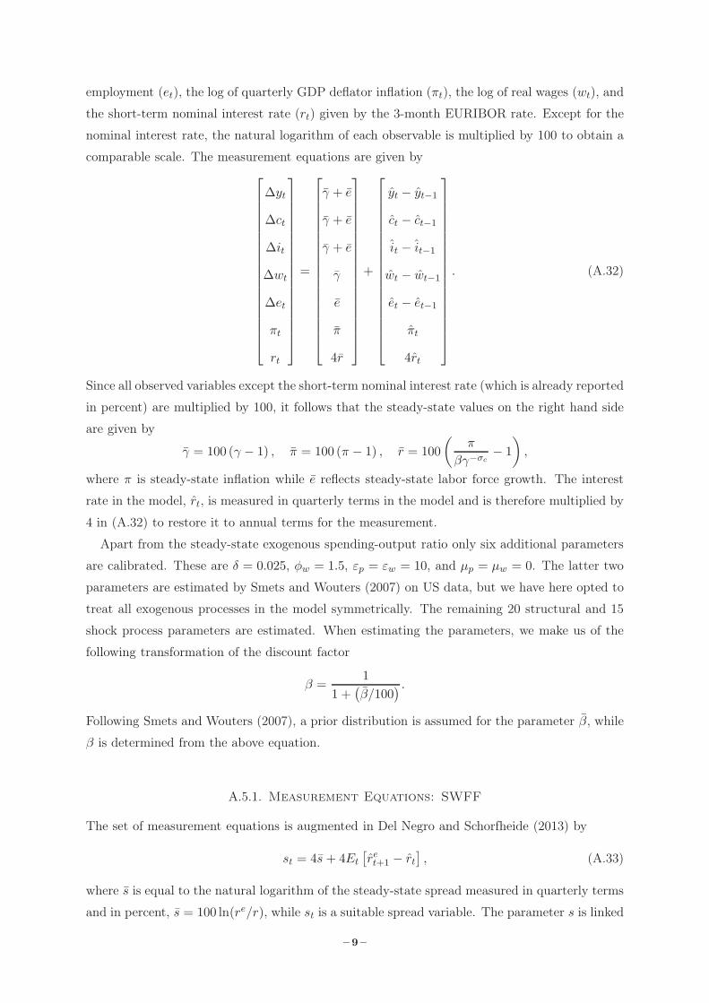
employment (et), the log of quarterly GDP deflator inflation (πt), the log of real wages (wt), and

the short-term nominal interest rate (rt) given by the 3-month EURIBOR rate. Except for the

nominal interest rate, the natural logarithm of each observable is multiplied by 100 to obtain a

comparable scale. The measurement equations are given by⎡⎢⎢⎢⎢⎢⎢⎢⎢⎢⎢⎢⎢⎢⎢⎢⎢⎢⎢⎣

∆yt

∆ct

∆it

∆wt

∆et

πt

rt

⎤⎥⎥⎥⎥⎥⎥⎥⎥⎥⎥⎥⎥⎥⎥⎥⎥⎥⎥⎦

=

⎡⎢⎢⎢⎢⎢⎢⎢⎢⎢⎢⎢⎢⎢⎢⎢⎢⎢⎢⎣

γ + e

γ + e

γ + e

γ

e

π

4r

⎤⎥⎥⎥⎥⎥⎥⎥⎥⎥⎥⎥⎥⎥⎥⎥⎥⎥⎥⎦

+

⎡⎢⎢⎢⎢⎢⎢⎢⎢⎢⎢⎢⎢⎢⎢⎢⎢⎢⎢⎣

yt − yt−1

ct − ct−1

it − it−1

wt − wt−1

et − et−1

πt

4rt

⎤⎥⎥⎥⎥⎥⎥⎥⎥⎥⎥⎥⎥⎥⎥⎥⎥⎥⎥⎦

. (A.32)

Since all observed variables except the short-term nominal interest rate (which is already reported

in percent) are multiplied by 100, it follows that the steady-state values on the right hand side

are given by

γ = 100 (γ − 1) , π = 100 (π − 1) , r = 100(

π

βγ−σc− 1

),

where π is steady-state inflation while e reflects steady-state labor force growth. The interest

rate in the model, rt, is measured in quarterly terms in the model and is therefore multiplied by

4 in (A.32) to restore it to annual terms for the measurement.

Apart from the steady-state exogenous spending-output ratio only six additional parameters

are calibrated. These are δ = 0.025, φw = 1.5, εp = εw = 10, and µp = µw = 0. The latter two

parameters are estimated by Smets and Wouters (2007) on US data, but we have here opted to

treat all exogenous processes in the model symmetrically. The remaining 20 structural and 15

shock process parameters are estimated. When estimating the parameters, we make us of the

following transformation of the discount factor

β =1

1 +(β/100

) .Following Smets and Wouters (2007), a prior distribution is assumed for the parameter β, while

β is determined from the above equation.

A.5.1. Measurement Equations: SWFF

The set of measurement equations is augmented in Del Negro and Schorfheide (2013) by

st = 4s + 4Et

[ret+1 − rt

], (A.33)

where s is equal to the natural logarithm of the steady-state spread measured in quarterly terms

and in percent, s = 100 ln(re/r), while st is a suitable spread variable. The parameter s is linked

– 9 –

to the steady-state values of the model variable variables according to

re

r= (1 + s/100)1/4 ,

r

π= β−1γσc ,

re

π= rk + 1 − δ.

If there are no financial frictions, then re = r, with the consequence that the steady-state

real interest rate is equal to the steady-state real rental rate on capital plus one minus the

depreciation rate of capital, i.e., the Smets and Wouters steady-state value; see Section A.4.

Del Negro and Schorfheide (2013) estimate s, ζsp,b, ρe, and σe while the parameters F and κe

are calibrated. The latter two parameters will appear in the next Section on the steady-state,

but it is useful to know that they represent the steady-state default probability and survival

rate of entrepreneurs, respectively, with F determined such that in annual terms the default

probability is 0.03 (0.0075 in quarterly terms) and κe = 0.99. These values are also used by

Del Negro et al. (2015). Finally, the financial frictions extension also involves the following

calibrated parameters: δ = 0.025, φw = 1.5, εp = εw = 10, and µp = µw = 0.

A.5.2. Measurement Equations: SWU

The steady-state values of the capital-output ratio, etc., are determined as in Section A.4 for the

SW model. The model is consistent with a BGP, driven by deterministic labor augmenting trend

growth, and the vector of observed variables for the euro area is augmented with an equation

for unemployment, denoted by ut. Specifically,

ut = u+ ut. (A.34)

The steady-state parameter u is given by

u = 100(φw − 1σl

), (A.35)

where (φw − 1) is the steady-state labor market markup and σl is the elasticity of labor supply

with respect to the real wage. Apart from the parameter σc, four additional structural param-

eters are calibrated. These are gy = 0.18, δ = 0.025, and εp = 10 as in the SW model. Unlike

Galí et al. (2012) and Smets et al. (2014) we estimate the persistence parameter of the labor

supply shock, ρs, and calibrate φw = 1.5. The latter parameter can also be estimated and yields

posterior mean and mode estimates very close to 1.5 when using the same prior as in Galí et al.

(2012) and Smets et al. (2014). We have opted to calibrate it in this study in order to treat it

in the same way across the three models.

– 10 –