Embed Size (px)
Citation preview
Calculus of Multivariables
1
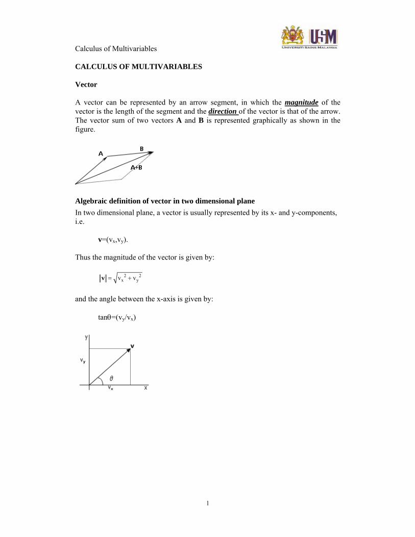
CALCULUS OF MULTIVARIABLES Vector A vector can be represented by an arrow segment, in which the magnitude of the vector is the length of the segment and the direction of the vector is that of the arrow. The vector sum of two vectors A and B is represented graphically as shown in the figure.
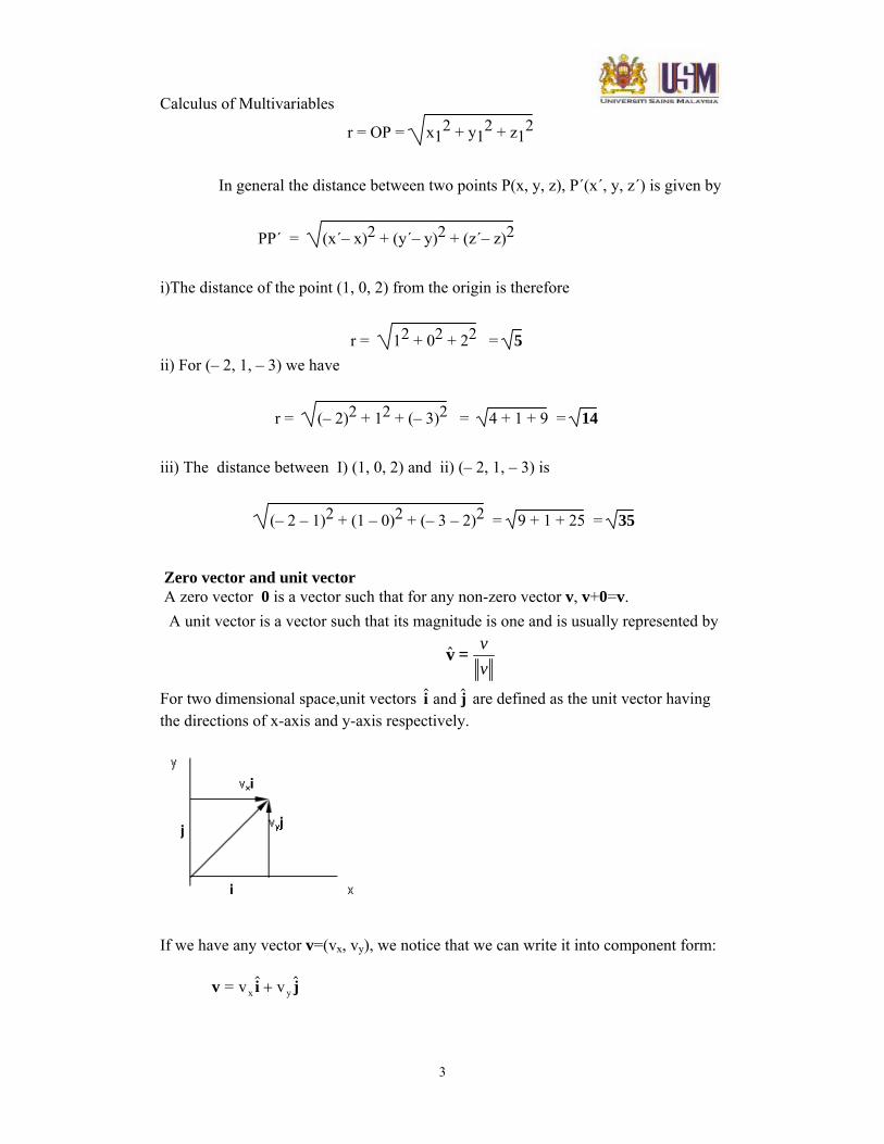
Algebraic definition of vector in two dimensional plane In two dimensional plane, a vector is usually represented by its x- and y-components, i.e.
v=(vx,vy).
Thus the magnitude of the vector is given by: 2 2
x yv v= +v and the angle between the x-axis is given by: tanθ=(vy/vx)

Calculus of Multivariables
2
Algebraic definition of vectors in three dimensional space
A vector v is defined in the three dimensional space by its x-, y- and z- components “ v=(vx,vy,vz) The magnitude of v is: 2 2 2
x y zv v v= + +v
x
y
z
o
(V , 0 , 0)x
(0 , V , 0)y
(0 , 0 , V )z
(V , V , V )x y z V
α
γβ
The angle α, β and γ are called the direction angles. The direction cosines of the vectors are defined by:
yx zvv v
cos , cos ,cosα β γ= = =v v v
Notice that: cos2α+cos2β+cos2γ=1. Example: Calculate the distances of the points i) (1, 0, 2), ii) (– 2, 1, – 3) from the origin. Also calculate the distance between each pair of points. Solution: The distance, r, from the origin O to the point P(x1, y1, z1) is given by
Calculus of Multivariables
3
r = OP = x12 + y1
2 + z12
In general the distance between two points P(x, y, z), P´(x´, y, z´) is given by
PP´ = (x´– x)2 + (y´– y)2 + (z´– z)2 i)The distance of the point (1, 0, 2) from the origin is therefore
r = 12 + 02 + 22 = 5 ii) For (– 2, 1, – 3) we have
r = (– 2)2 + 12 + (– 3)2 = 4 + 1 + 9 = 14
iii) The distance between I) (1, 0, 2) and ii) (– 2, 1, – 3) is
(– 2 – 1)2 + (1 – 0)2 + (– 3 – 2)2 = 9 + 1 + 25 = 35 Zero vector and unit vector A zero vector 0 is a vector such that for any non-zero vector v, v+0=v. A unit vector is a vector such that its magnitude is one and is usually represented by
ˆ vv
v =
For two dimensional space,unit vectors i jand are defined as the unit vector having the directions of x-axis and y-axis respectively.
If we have any vector v=(vx, vy), we notice that we can write it into component form: v i j= v vx y+
Calculus of Multivariables
4
Two dimensions ( ) ( ) ( )( ) ( ), , 0 0,
ˆ ˆ 1,0 0,1
v x y x y
x y x i y j
= = +
= + = +
Similar to the two dimensional space, unit vectors parallel to the x-, y- and z-axis are defined as:
Three dimensions ( ) ( ) ( )( )( ) ( ) ( ), , ,0,0 0, ,0 0,0,
ˆˆ ˆ 1,0,0 0,1,0 0,0,1
v x y z x y z
x y z x i y j z k
= = + +
= + + = + +
(0,0,1)ˆ and (0,1,0)ˆ (1,0,0);ˆ === kji and thus,
kjiv ˆvˆvˆv)v,v,(v zyxzyx ++== Example: If v=2 i -3 j is a vector, find the unit vector which has the same direction as that of v. Solution:
2 22 3 13= + =v
Unit vector which has the same direction as that of v is
ˆ ˆ2i-3jˆ13
vv
=v =
Practice 1: Calculate the magnitude and direction for each of the position vectors:- i) a = 3i ii) b = i + j iii) c = 3i – 3j iv) d = 3 i + j v) e = i + 2 j Find unit vectors in the direction of each vector. Addition and scalar multiplication of vector Geometric vector addition: Arrange the vectors head to tail. The sum is the vector beginning with tail of the first vector and ending with the sum of the last vector. Use the law of sines and the law of cosines to solve for the length of the vector the angle.
ba)sin()sin( βα
= and )cos(2222 γabbac −+=
Algebraic vector addition: Two dimensions: If necessary break the vectors into x-components and y-components
Calculus of Multivariables
5
)sin(
)cos(
θ
θ
⋅=
⋅=
vy
vx.
Combine the x-components and y-components separately ),( 212121 yyxxvv ++=+ .
Three dimensions: ),,( 21212121 zzyyxxvv +++=+ .
Scalar multiplication: If u=(ux, uy), v=(vx, vy) and α is a scalar then (i) u+v=(ux+vx, uy+vy) (ii) αu=(αux, αuy) (iii) –u=(-ux, -uy) (iv) u-v=u+(-v)=(ux-vx, uy-vy) Theorem : Algebraic properties of vector ,if u, v and w are vectorsα and β are two scalars and 0 is the zero vector (i) u+v=v+u (ii) u+(v+w)=(u+v)+w (iii) v+(-v)=0 (iv) (αβv)=α(βv) (v) (α+β)v=αv+βv (vi) α(u+v)=αu+αv (vii) ⏐αv⏐=α⏐v⏐ Dot product Dot product of two vector u=ux i +uy j and v=vx i +vy j is a scalar and is defined as: u•v=uxvx+uyvy Multiply two vectors to obtain a scalar. Defined for n-dimensional space. Two dimensions numberyyxxvv =⋅+⋅=⋅ 212121 Three dimensions numberzzyyxxvv =⋅+⋅+⋅=⋅ 21212121
. )cos( 212121 vandvbetweenanglepositivesmallesttheiswherevvvv θθ⋅=⋅ Length of a vector: vvv ⋅=
Angle between two vectors: 21
21)cos(vvvv ⋅
=θ
Calculus of Multivariables
6
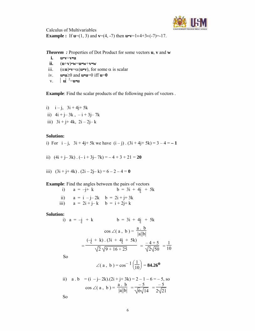
Example : If u=(1, 3) and v=(4, -7) then u•v=1×4+3×(-7)=-17.
Theorem : Properties of Dot Product for some vectors u, v and w i. u•v=v•u
ii. (u+v)•w=u•w+v•w iii. (αu)•v=α(u•v), for some α is scalar iv. u•u≥0 and u•u=0 iff u=0 v. ⏐u⏐2=u•u
Example: Find the scalar products of the following pairs of vectors . i) i – j, 3i + 4j+ 5k ii) 4i + j– 3k , – i + 3j– 7k iii) 3i + j+ 4k, 2i – 2j– k Solution: i) For i – j, 3i + 4j+ 5k we have (i – j) . (3i + 4j+ 5k) = 3 – 4 = – 1 ii) (4i + j– 3k) . (– i + 3j– 7k) = – 4 + 3 + 21 = 20 iii) (3i + j+ 4k) . (2i – 2j– k) = 6 – 2 – 4 = 0
Example: Find the angles between the pairs of vectors i) a = –j+ k b = 3i + 4j- + 5k
ii) a = i – j– 2k b = 2i + j+ 3k iii) a = 2i + j– k b = i + 2j+ k Solution: i) a = –j- + k b = 3i + 4j- + 5k
cos ∠( a , b ) = a . b | |a | |b
= (–j- + k) . (3i + 4j- + 5k)
2 9 + 16 + 25 =
– 4 + 52 50
= 1
10
So
∠( a , b ) = cos– 1 ⎝⎜⎛
⎠⎟⎞1
10 = 84.26o
ii) a . b = (i – j– 2k).(2i + j+ 3k) = 2 – 1 – 6 = – 5, so
cos ∠( a , b ) = a . b | |a | |b =
– 56 14
= – 5
2 21
So
Calculus of Multivariables
7
∠( a , b ) = 180° – cos– 1 ⎝⎜⎛
⎠⎟⎞5
2 21 = 123.06o
iii) a . b = (2i + j– k ).(i + 2j+ k) = 2 + 2 – 1 = 3 so
cos ∠( a , b ) = a . b | |a | |b =
36 =
12
So
∠( a , b ) = cos– 1 ⎝⎜⎛⎠⎟⎞1
2 = 60o
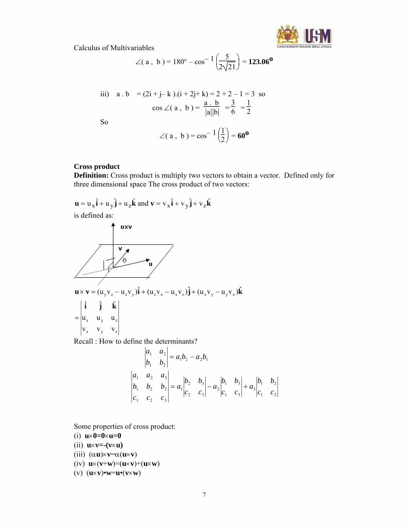
Cross product Definition: Cross product is multiply two vectors to obtain a vector. Defined only for three dimensional space The cross product of two vectors:
kjiv kjiu ˆvˆvˆv andˆuˆuˆu zyxzyx ++=++= is defined as:
zyx
zyx
xyyxzxxzyzzy
vvvuuu
ˆˆˆ
ˆ)vuv(uˆ)vuv(uˆ)vuv(u
kji
kjivu
=
−+−+−=×
Recall : How to define the determinants?
21
213
31
312
32
321
321
321
321
122121
21
ccbb
accbb
accbb
acccbbbaaa
bababbaa
+−=
−=
Some properties of cross product: (i) u×0=0×u=0 (ii) u×v=-(v×u) (iii) (αu)×v=α(u×v) (iv) u×(v+w)=(u×v)+(u×w) (v) (u×v)•w=u•(v×w)
Calculus of Multivariables
8
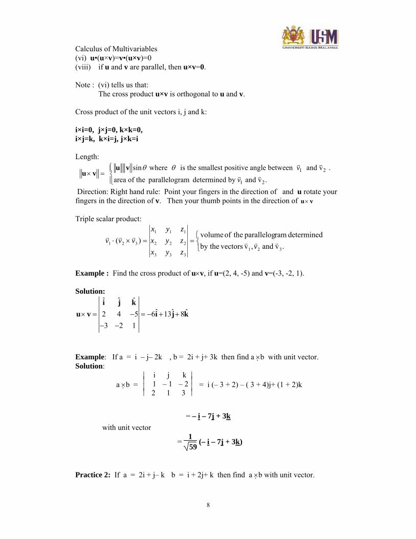
(vi) u•(u×v)=v•(u×v)=0 (viii) if u and v are parallel, then u×v=0.
Note : (vi) tells us that: The cross product u×v is orthogonal to u and v. Cross product of the unit vectors i, j and k: i×i=0, j×j=0, k×k=0, i×j=k, k×i=j, j×k=i Length:
1 2
1 2
sin where is the smallest positive angle between and v .
area of the parallelogram determined by and v . v
vθ θ⎧⎪× = ⎨
⎪⎩
u vu v
Direction: Right hand rule: Point your fingers in the direction of and u rotate your fingers in the direction of v. Then your thumb points in the direction of ×u v Triple scalar product:
⎩⎨⎧
==×⋅.v and ,v vectorsby the
determined ramparallelog theof volume)(
321333
222
111
321 vzyxzyxzyx
vvv
Example : Find the cross product of u×v, if u=(2, 4, -5) and v=(-3, -2, 1).
Solution:
ˆ ˆ ˆˆ ˆ ˆ2 4 5 6 13 8
3 2 1× = − = − + +
− −
i j ku v i j k
Example: If a = i – j– 2k , b = 2i + j+ 3k then find a ×b with unit vector. Solution:
a ×b = ⎪⎪⎪⎪
⎪⎪⎪⎪ i j k
1 – 1 – 22 1 3
= i (– 3 + 2) – ( 3 + 4)j+ (1 + 2)k
= – i – 7j + 3k
with unit vector
= 159
(– i – 7j + 3k)
Practice 2: If a = 2i + j– k b = i + 2j+ k then find a ×b with unit vector.
Calculus of Multivariables
9
Practice 3: If a = 3i – 2 j_ + k , b = i + j_ + k and c = 2i + j_ – 3k
evaluate: a . b × c
Vector Gradient
The gradient of a (scalar) function ( )yxff ,= is defined by
( ) ( ) ( )ji yxfyxfyxf yx ,,, +=∇ .
As we can see, the gradient of a function is a vector field. It is the vector field which
will points in the direction of the greatest rate of change of the function f. The
magnitude of the gradient is the greatest rate of change.
Example
Find the gradient of ( ) yyxyxf 3, 2 += .
Solution
The gradient of f is ( )jiji 32 2 ++=+=∇ xxyfff yx .
Functions of several variables Definition: A function f of two variables is a rule that assigns to each ordered pair of real numbers ),( yx in a set D a unit real number denoted by ).,( yxf The set D is the domain of f is the set of values that f takes on, that is, { }.),(),( Dyxyxf ∈ ),( yxfz = maps each ordered pair ),( yx to a unique number z . ),,( zyxfw = maps each ordered triple ),,( zyx to a unique number w . Example : Find the domains of the following functions and evaluate ).2,3(f
(a) 1
1),(
−++
=x
yxyxf
Solution: This function is not defined whenever ,1=x so the domain does not include all the
points on the plane .1=x
Calculus of Multivariables
10
We consider the expression 1++ yx . This expression is not defined for
01 ≤++ yx or .1−≤+ yx
Example: Find the domain and range of
229),( yxyxg −−= Solution:
The function g is defined only for 09 22 ≥−− yx which is equivalent to
922 ≤+ yx , so the domain
}9:),{(}09:),{( 2222 ≤+=≥−−= yxyxyxyxD
Practice 4: Determine the domain of each of the following.
i) ( , )g x y x y= +
ii) ( , )g x y x y= +
iii) 2 2( , ) (9 9 )g x y In x y= − −
GRAPH: QUADRIC SURFACES
Definition If f is a function of two variables with domain D, then the graph of f is the
set of points ),,( zyx in 3R such that ),( yxfz = and ),( yx is in D.
LEVEL CURVES AND SURFACES
• Level curves The level curves of ),( yxfz = have equations kyxf =),( .
),( yxfz = describes a surface above and/or below the x-y plane. If the surface is cut by the horizontal plane kz = and the resulting curve is projected onto the x-y plane we obtain the level curve of height k. • Level surfaces The level surfaces of ),,( zyxfw = have equations kzyxf =),,( . If ),,( zyxf assigned a temperature to each point in space, then the level surfaces would be surfaces of constant temperature.
Calculus of Multivariables
11
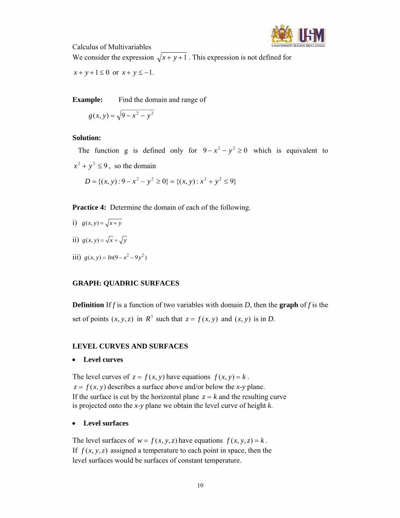
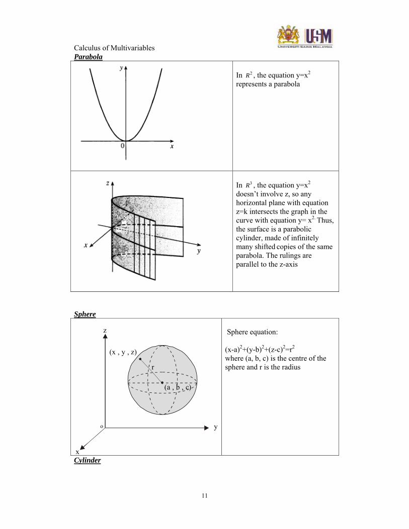
Parabola
In 2R , the equation y=x2 represents a parabola
In 3R , the equation y=x2 doesn’t involve z, so any horizontal plane with equation z=k intersects the graph in the curve with equation y= x2. Thus, the surface is a parabolic cylinder, made of infinitely many shifted copies of the same parabola. The rulings are parallel to the z-axis
Sphere
Sphere equation: (x-a)2+(y-b)2+(z-c)2=r2 where (a, b, c) is the centre of the sphere and r is the radius
Cylinder
x
y
z
o
(x , y , z)
(a , b , c)
r
Calculus of Multivariables
12
x
y
z
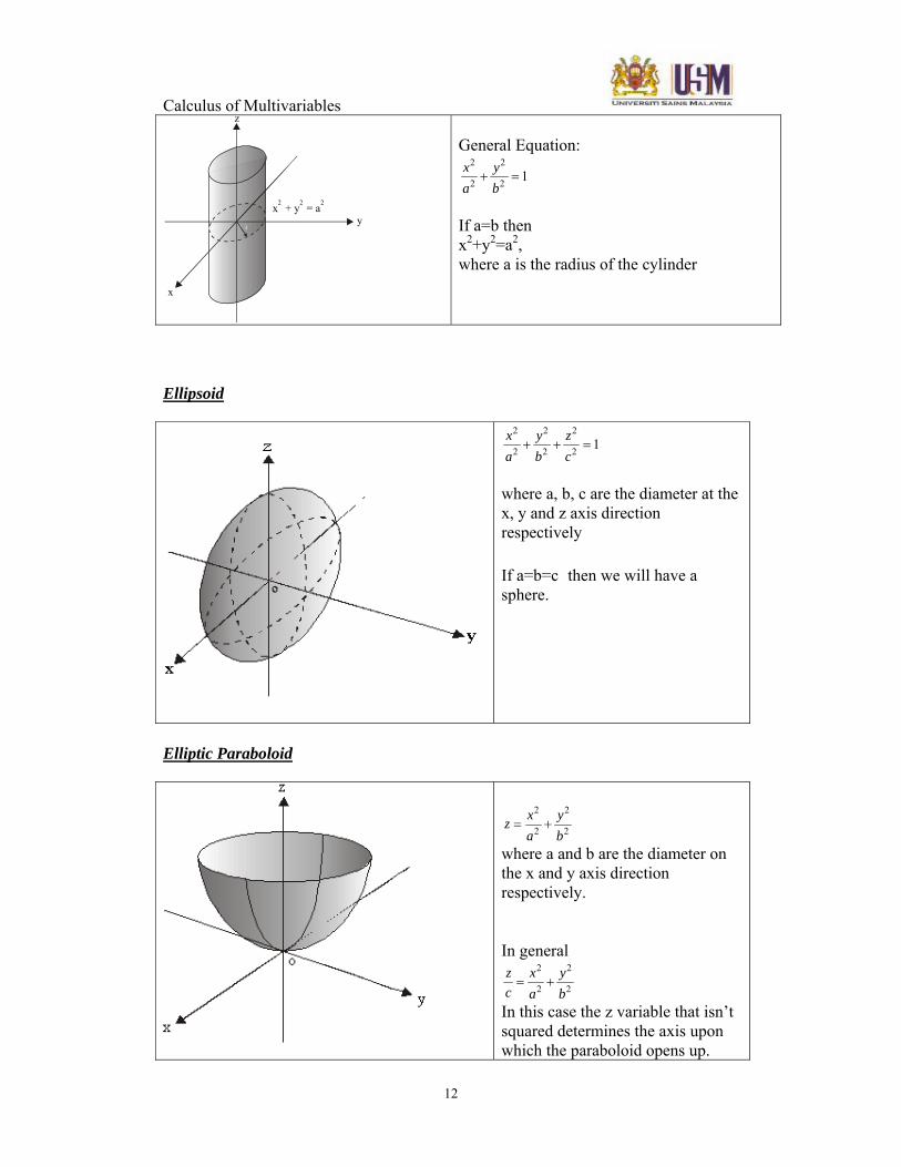
x + y = a2 2 2
General Equation:
2 2
2 2 1x ya b
+ =
If a=b then x2+y2=a2, where a is the radius of the cylinder
Ellipsoid
2 2 2
2 2 2 1x y za b c
+ + =
where a, b, c are the diameter at the x, y and z axis direction respectively If a=b=c then we will have a sphere.
Elliptic Paraboloid
2 2
2 2x yza b
= +
where a and b are the diameter on the x and y axis direction respectively. In general
2 2
2 2z x yc a b= +
In this case the z variable that isn’t squared determines the axis upon which the paraboloid opens up.
Calculus of Multivariables
13
Also, the sign of c will determine the direction that the paraboloid opens. If c is positive then it opens up and if c is negative then it opens down.
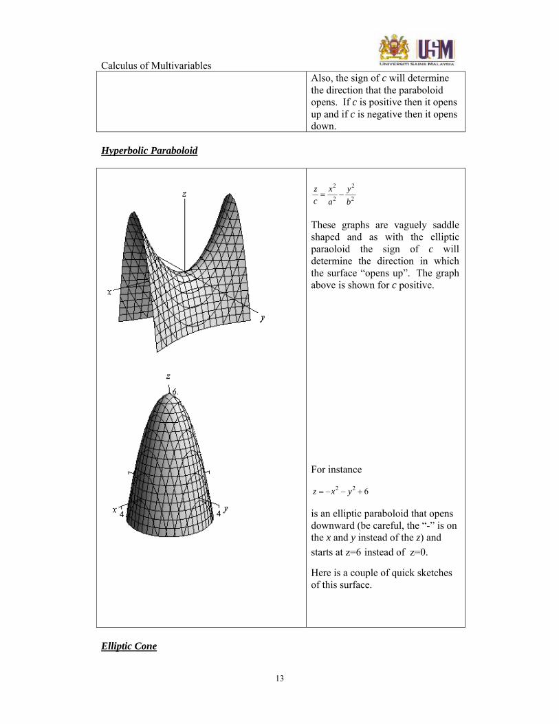
Hyperbolic Paraboloid
2 2
2 2z x yc a b= −
These graphs are vaguely saddle shaped and as with the elliptic paraoloid the sign of c will determine the direction in which the surface “opens up”. The graph above is shown for c positive.
For instance
2 2 6z x y= − − +
is an elliptic paraboloid that opens downward (be careful, the “-” is on the x and y instead of the z) and starts at z=6 instead of z=0.
Here is a couple of quick sketches of this surface.
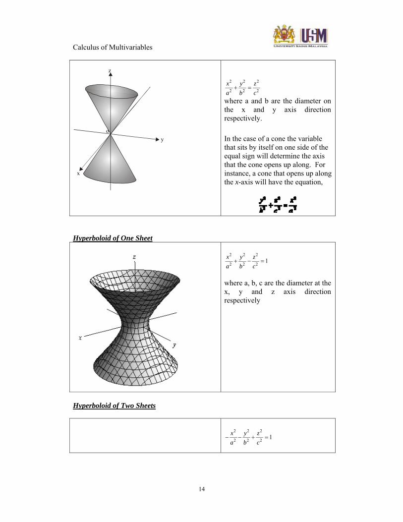
Elliptic Cone
Calculus of Multivariables
14
x
y
z
o
2 2 2
2 2 2x y za b c
+ =
where a and b are the diameter on the x and y axis direction respectively. In the case of a cone the variable that sits by itself on one side of the equal sign will determine the axis that the cone opens up along. For instance, a cone that opens up along the x-axis will have the equation,
Hyperboloid of One Sheet
2 2 2
2 2 2 1x y za b c
+ − =
where a, b, c are the diameter at the x, y and z axis direction respectively
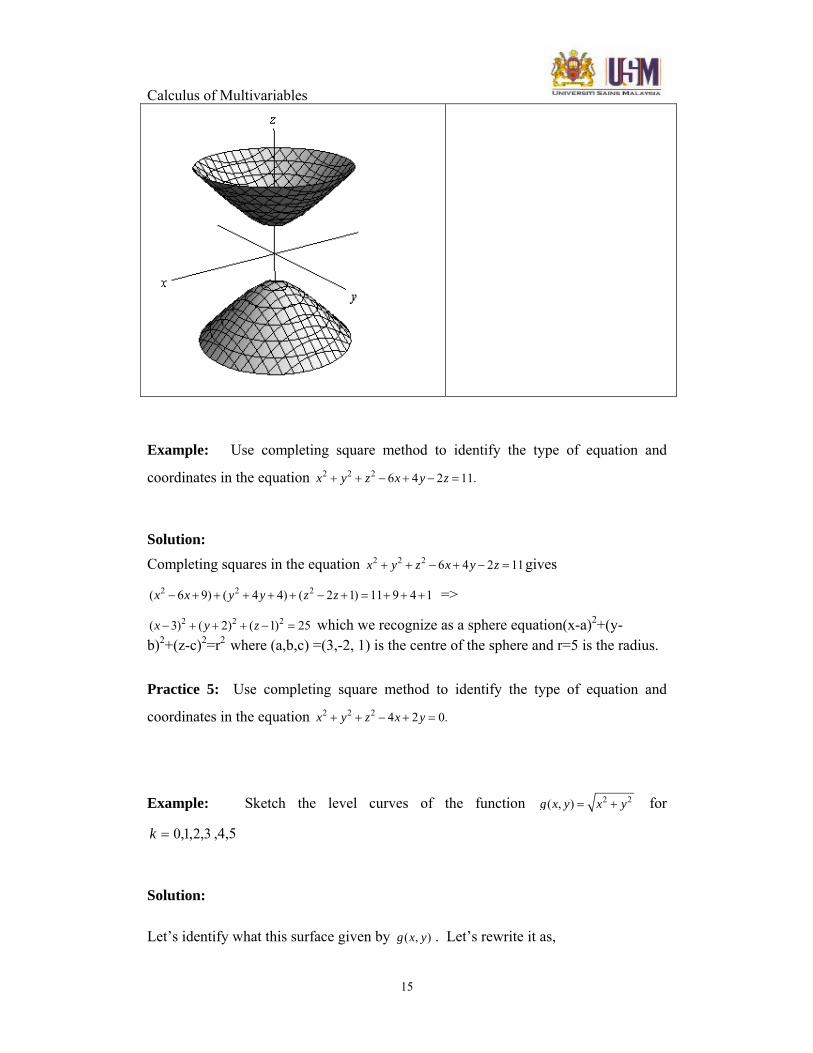
Hyperboloid of Two Sheets
2 2 2
2 2 2 1x y za b c
− − + =
Calculus of Multivariables
15
Example: Use completing square method to identify the type of equation and
coordinates in the equation 2 2 2 6 4 2 11.x y z x y z+ + − + − =
Solution:
Completing squares in the equation 2 2 2 6 4 2 11x y z x y z+ + − + − = gives 2 2 2( 6 9) ( 4 4) ( 2 1) 11 9 4 1x x y y z z− + + + + + − + = + + + =>
2 2 2( 3) ( 2) ( 1) 25x y z− + + + − = which we recognize as a sphere equation(x-a)2+(y-b)2+(z-c)2=r2 where (a,b,c) =(3,-2, 1) is the centre of the sphere and r=5 is the radius.
Practice 5: Use completing square method to identify the type of equation and
coordinates in the equation 2 2 2 4 2 0.x y z x y+ + − + =
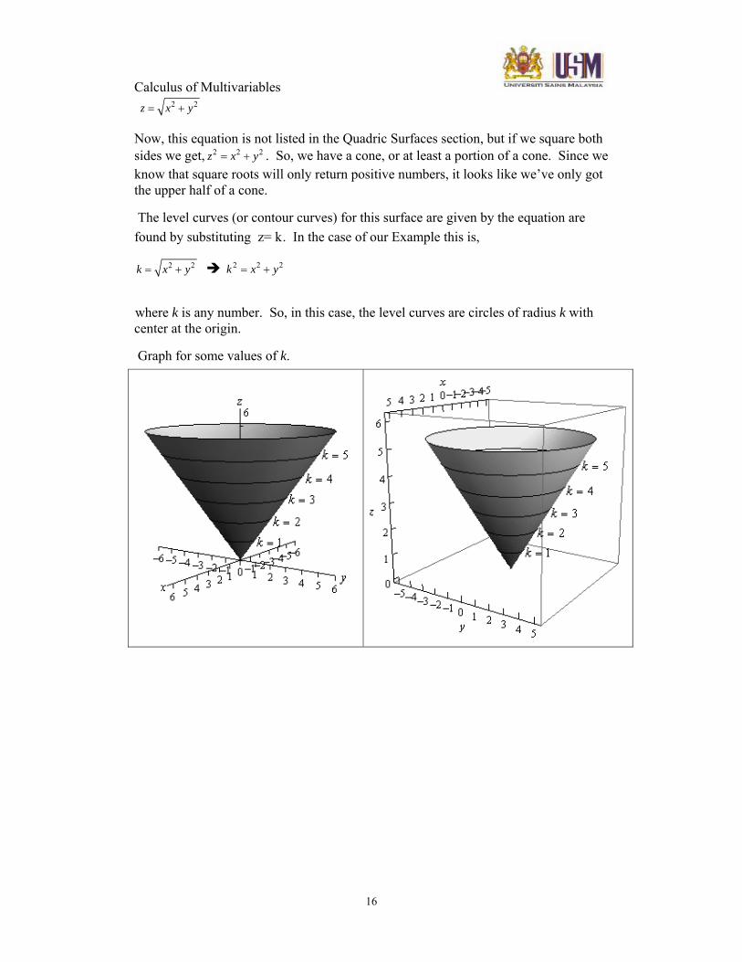
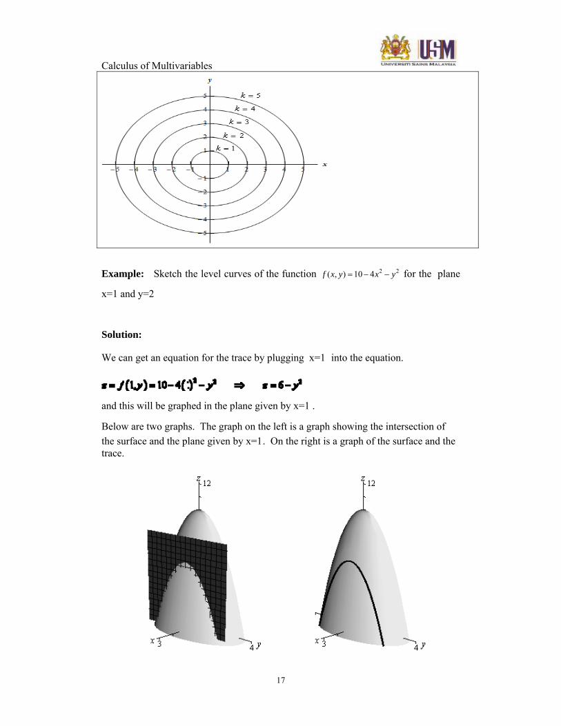
Example: Sketch the level curves of the function 2 2( , )g x y x y= + for
3,2,1,0=k ,4,5
Solution:
Let’s identify what this surface given by ( , )g x y . Let’s rewrite it as,
Calculus of Multivariables
16
2 2z x y= +
Now, this equation is not listed in the Quadric Surfaces section, but if we square both sides we get, 2 2 2z x y= + . So, we have a cone, or at least a portion of a cone. Since we know that square roots will only return positive numbers, it looks like we’ve only got the upper half of a cone.
The level curves (or contour curves) for this surface are given by the equation are found by substituting z= k. In the case of our Example this is,
2 2k x y= + 2 2 2k x y= +
where k is any number. So, in this case, the level curves are circles of radius k with center at the origin.
Graph for some values of k.
Calculus of Multivariables
17
Example: Sketch the level curves of the function 2 2( , ) 10 4f x y x y= − − for the plane
x=1 and y=2
Solution:
We can get an equation for the trace by plugging x=1 into the equation.
and this will be graphed in the plane given by x=1 .
Below are two graphs. The graph on the left is a graph showing the intersection of the surface and the plane given by x=1. On the right is a graph of the surface and the trace.
Calculus of Multivariables
18
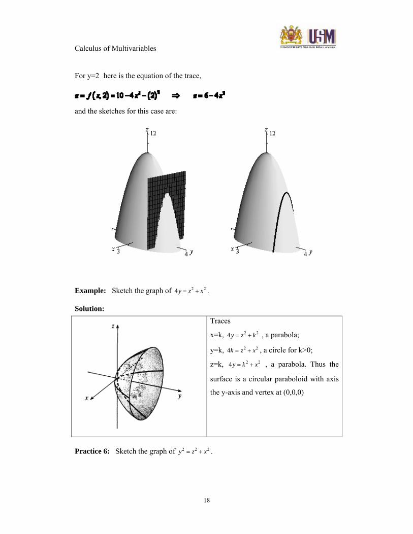
For y=2 here is the equation of the trace,
and the sketches for this case are:
Example: Sketch the graph of 2 24y z x= + .
Solution:
Traces
x=k, 2 24y z k= + , a parabola;
y=k, 2 24k z x= + , a circle for k>0;
z=k, 2 24y k x= + , a parabola. Thus the
surface is a circular paraboloid with axis
the y-axis and vertex at (0,0,0)
Practice 6: Sketch the graph of 2 2 2y z x= + .
Calculus of Multivariables
19
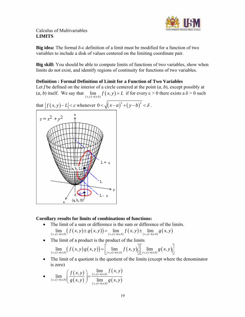
LIMITS Big idea: The formal δ-ε definition of a limit must be modified for a function of two variables to include a disk of values centered on the limiting coordinate pair. Big skill: You should be able to compute limits of functions of two variables, show when limits do not exist, and identify regions of continuity for functions of two variables. Definition : Formal Definition of Limit for a Function of Two Variables Let f be defined on the interior of a circle centered at the point (a, b), except possibly at (a, b) itself. We say that
( ) ( )( )
, ,lim ,
x y a bf x y L
→= if for every ε > 0 there exists a δ > 0 such
that ( ),f x y L ε− < whenever ( ) ( )2 20 x a y b δ< − + − < .
Corollary results for limits of combinations of functions:
• The limit of a sum or difference is the sum or difference of the limits.
( ) ( )( ) ( )( )
( ) ( )( )
( ) ( )( )
, , , , , ,lim , , lim , lim ,
x y a b x y a b x y a bf x y g x y f x y g x y
→ → →± = ±
• The limit of a product is the product of the limits
( ) ( )( ) ( )( )
( ) ( )( )
( ) ( )( )
, , , , , ,lim , , lim , lim ,
x y a b x y a b x y a bf x y g x y f x y g x y
→ → →
⎡ ⎤ ⎡ ⎤= ⎢ ⎥ ⎢ ⎥⎣ ⎦ ⎣ ⎦
• The limit of a quotient is the quotient of the limits (except where the denominator is zero)
• ( ) ( )
( )( )
( ) ( )( )
( ) ( )( )
, ,
, ,, ,
lim ,,lim
, lim ,x y a b
x y a bx y a b
f x yf x yg x y g x y
→
→→
⎛ ⎞=⎜ ⎟⎜ ⎟
⎝ ⎠
Calculus of Multivariables
20
• The limit of a polynomial always exists and is found simply by substitution.
( ) ( )( )( ) ( )
, ,lim , ,n nx y a b
P x y P a b→
=
Notes on disproving limits:
• For a limit to exist, the function must approach that limit for every possible path of (x, y) approaching (a, b). Thus, it is usually very hard to prove a limit exists, and easier to show a limit does not exist. • So, if a function f(x, y) approaches L1 as (x, y) approaches (a, b) along a path P1 and f(x, y) approaches L2 ≠ L1 as (x, y) approaches (a, b) along a different path P2, then
( ) ( )( )
, ,lim ,
x y a bf x y
→ does not exist.
• Some simple paths to try are the lines along x = a, y = b, or any other line through the point.
Example:
Evaluate ( ) ( )
2
2, 2,1
2 3lim5 3x y
x y xyxy y→
++
Solution:
( ) ( )
2 2
2 2, 2,1
2 3 2(2) (1) 3(2)(1) 14lim5 3 5(2)(1) 3(1) 13x y
x y xyxy y→
+ += =
+ +
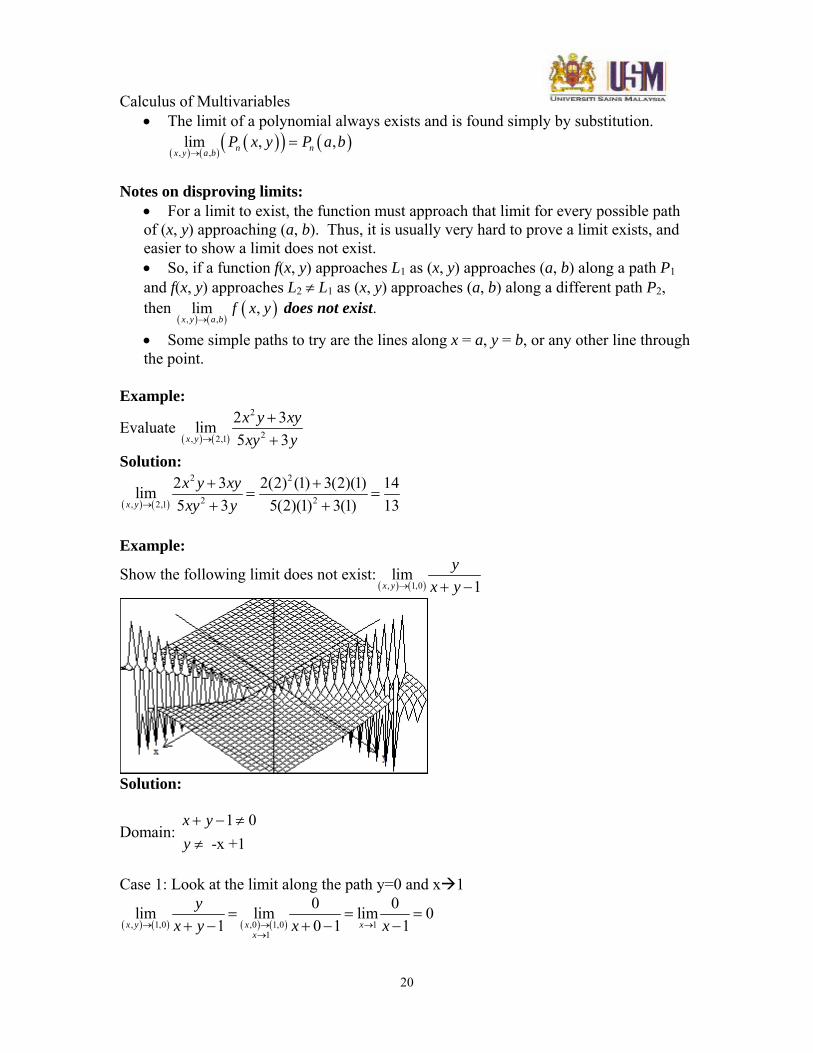
Example:
Show the following limit does not exist:( ) ( ), 1,0
lim1x y
yx y→ + −
Solution:
Domain: 1 0
-x +1x yy+ − ≠≠
Case 1: Look at the limit along the path y=0 and x 1
( ) ( ) ( ) ( ), 1,0 ,0 1,0 1 1
0 0lim lim lim 01 0 1 1x y x x
x
yx y x x→ → →
→
= = =+ − + − −
Calculus of Multivariables
21
Case 2: Look at the limit along the path x=1 and y 0
( ) ( ) ( ) ( ), 1,0 1, 1,0 0 y 0
lim lim lim 11 1 1x y y y
y y yx y y y→ → →
→
= = =+ − + −
The original limit does not exist
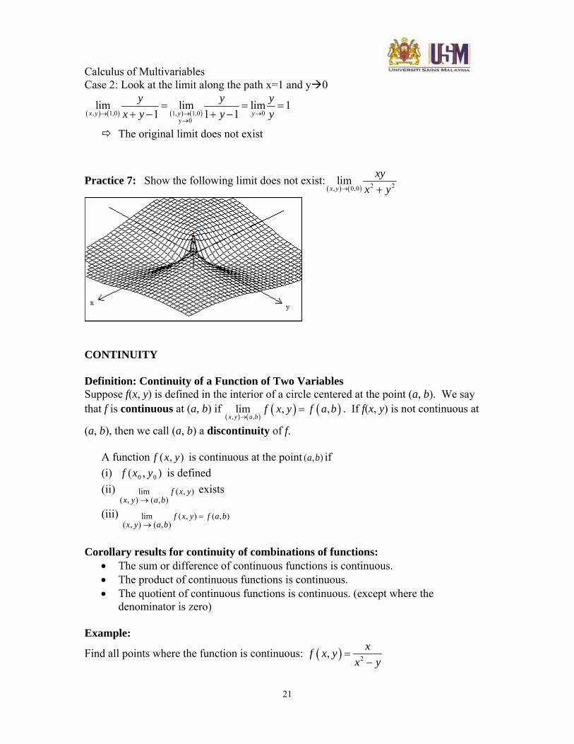
Practice 7: Show the following limit does not exist:( ) ( ) 2 2, 0,0
limx y
xyx y→ +
CONTINUITY Definition: Continuity of a Function of Two Variables Suppose f(x, y) is defined in the interior of a circle centered at the point (a, b). We say that f is continuous at (a, b) if
( ) ( )( ) ( )
, ,lim , ,
x y a bf x y f a b
→= . If f(x, y) is not continuous at
(a, b), then we call (a, b) a discontinuity of f. A function ),( yxf is continuous at the point ( , )a b if
(i) ),( 00 yxf is defined (ii) lim ( , )
( , ) ( , )f x y
x y a b→ exists
(iii) lim ( , ) ( , )( , ) ( , )
f x y f a bx y a b
=→
Corollary results for continuity of combinations of functions:
• The sum or difference of continuous functions is continuous. • The product of continuous functions is continuous. • The quotient of continuous functions is continuous. (except where the
denominator is zero) Example:
Find all points where the function is continuous: ( ) 2, xf x yx y
=−

Calculus of Multivariables
22
xy
Solution:
(i) 2 2f(a,b) is defined except where x -y=0 or y= x is discontinuous
(ii) 2 2lim ( , ) exists except where x -y=0 or y= x is discontinuous ( , ) ( , )
f x yx y a b→
(iii) 2 2lim ( , ) ( , ) except where x -y=0 or y= x is discontinuous ( , ) ( , )
f x y f a bx y a b
=→
Therefore 2( , ) is for {( , ) | x }f x y continuous x y y ≠
Practice 8: Find all points where the function is continuous:
( ) ( ) ( )
( ) ( )
2
2 2 if , 0,0,
0 if , 0,0
x y x yx yf x y
x y
⎧≠⎪ += ⎨
⎪ =⎩
Calculus of Multivariables
23
PARTIAL DIFFERENTIAL EQUATIONS
Definition: Consider a function f(x,y) of two variables. If we treat y as a constant, f may be differentiated with respect to x. The result is called the partial derivative of f with
respect to x and is denoted by fx or dxdf . If we let z = f(x,y), we write fx =
dxdz . The partial
derivative with respect to y is similarly defined by treating x as constant and differentiating f(x,y) with respect to y. • Differentiability A function is differentiable if it possesses the property of local linearity. For functions of two variables this means we can accurately approximate the surface using a tangent plane. Definition: A function ),( yxf is differentiable at the point ),( 00 yx if
),( 00 yxxf∂∂ and ),( 00 yx
yf∂∂ exist and fΔ can be written as
yxyyxyfxyx
xff Δ+Δ+Δ
∂∂
+Δ∂∂
=Δ 210000 ),(),( εε
where 0, 21 →εε as )0,0(),( →ΔΔ yx . • First partials
hyxfhyxfyx
yf
hyxfyhxfyx
xf
h
h
),(),(lim),(
),(),(lim),(
0
0
−+=
∂∂
−+=
∂∂
→
→
We can interpret partial derivatives as rates of change. If ),( yxfz = , then xz ∂∂ /
represents the rate of change of z with respect to x when y is fixed. Similarly, yz ∂∂ / is
the rate of change of z with respect to y when x is fixed.
Theorem: If ),( yxf has continuous first partial derivatives in a neighborhood of ),( 00 yx then ),( yxf is differentiable at the point ),( 00 yx . Theorem: Differentiability ⇒ continuity.
Calculus of Multivariables
24
Example: i) If f(x,y) = xy + excos y, compute fx and fy. ii) For f as in (a), calculate fx(1,π/2). Solution i) Treating y as a constant and differentiating with respect to x, we get fx(x,y) = y + excos y. Differentiating with respect y and considering x as a constant gives fy(x,y) = x – exsin y. ii) Substituting x = 1 and y = π/2, we get fx(1,π/2) =π/2 + e1cos(π/2) = π/2. Practice 9:
i) If 24332 xyeyxyxz −+= , calculate
dxdz and
dydz
.
ii) If ,24),( 22 yxyxf −−= find )1,1(xf and ).1,1(yf
iii) Show that the function yeyxu x sin),( = is a solution of Laplace’s equation.
02
2
2
2
=∂∂
+∂∂
yu
xu is called Laplace equation.
• Increments
),(),( yxfyyxxff −Δ+Δ+=Δ is called the increment of f and is the actual change in the function f as ),( yx is moved to ),( yyxx Δ+Δ+ . • Total differentials
yyfx
xfdf Δ
∂∂
+Δ∂∂
= is called the total differential of f and is the tangent plane
approximation to the change in f as ),( yx is moved to ),( yyxx Δ+Δ+ . The ( ) ( ), ,x ydf f x y dx f x y dy= +
total differential is actually the equation for the tangent plane in local coordinates centered at the point of tangency.
Calculus of Multivariables
25
The total differential of f x y z( , , ) is defined by the equation
d ffx
d xfy
d yfz
d z= + +∂∂
∂∂
∂∂
whether or not x, y and z are independent of each other, provided only that the partial derivatives involved are continuous. Example: (a) If z = f(x,y) = x2 + 3xy – y2 , find the differential dz.
(b) If x changes from 2 to 2.05 and y changes from 3 to 2.96, compare the value of Δz and dz.
Solution
(a) dyyxdxyxdyyzdx
xzdz )23()32( −++=
∂∂
+∂∂
= .
(b) Putting x = 2, dx = Δx = 0.05, y = 3, and dy = Δy = - 0.04, we get dz = [2(2) + 3(3)]0.05 + [3(2) - 2(3)](- 0.04) = 0.65
The increment of z is Δz = f(2.05,2.96) - f(2,3) = [(2.05)2 + 3(2.05)(2.96) - (2.96)2 ] - [22 + 3(2)(3) – 32 ] = 0.6449
Notice that Δz = dz but dz is easier to compute.
HIGHER DERIVATIVES
If ),,( yxfz = we use the following notations.
xxfxf
xf
x=
∂∂
=⎟⎠⎞
⎜⎝⎛∂∂
∂∂
2
2
yxfyxf
yf
x=
∂∂∂
=⎟⎟⎠
⎞⎜⎜⎝
⎛∂∂
∂∂ 2
xyfxyf
xf
y=
∂∂∂
=⎟⎠⎞
⎜⎝⎛∂∂
∂∂ 2
yyfyf
yf
y=
∂∂
=⎟⎟⎠
⎞⎜⎜⎝
⎛∂∂
∂∂
2
2
Clairut’s Theorem Suppose f is defined on a disk D that contains the points ).,( ba If the functions xyf and yxf are both continuous on D, then ),(),( bafbaf yxxy = or
∂∂ ∂
∂∂ ∂
2 2fy x
fx y
= or f fyx xy=
Calculus of Multivariables
26
if the derivatives involved are continuous.
THE CHAIN RULE
The Chain Rule (Case 1) One independent variable ),( yxfz = is a differentiable functions of x and y, where )(tgx = and )(thy = are both differentiable functions of t.
Then z is a differentiable function of t anddtdy
yf
dtdx
xf
dtdz
∂∂
+∂∂
=
Example:
If ,sin,cos22 teytexandyxu tt ==−= find dtdu
Solution:
dtdy
yu
dtdx
xu
dtdu
∂∂
+∂∂
=
( ) ( )( )( ) ( )
[ ]( )( ).2sin2cos2
2sinsincos2cossin2sin2sincos2cos2
cossinsin2sincoscos2cossin2sincos2
2
222
222
ttettte
ttttttetetetetetete
teteytetex
t
t
t
tttttt
tttt
−=
−−=
−−−=
+−−=
+−+−=
Practice 10: If ,3 42 xyyxz += where tx 2sin= and ty cos= , find dtdz / when .0=t
Practice 11: The pressure P (in kilopascals), volume V (in liters), and tempreture T (in kelvins) of a
mole of an ideal gas are related by the equation .31.8 TPV = Find the rate at which the
pressure is changing when the tempreture is 300 K and increasing at a rate 0.1 K/s and
the volume is 100 L and increasing at a rate of 0.2 L/s.
The Chain Rule (Case 2): Two independent variables ),( yxfz = is a differentiable
functions of x and y, where ),( tsgx = and ),( tshy = are both differentiable functions of
s and t. Then z is a differentiable function of t and
Calculus of Multivariables
27
sy
yz
sx
xz
sz
∂∂
∂∂
+∂∂
∂∂
=∂∂
ty
yz
tx
xz
tz
∂∂
∂∂
+∂∂
∂∂
=∂∂
Example: If ,sin yez x= where 2stx = and tsy 2= , find sz ∂∂ / and tz ∂∂ / . Solution:
Since the Chain Rule gives
sy
yz
sx
xz
sz
∂∂
∂∂
+∂∂
∂∂
=∂∂ and
ty
yz
tx
xz
tz
∂∂
∂∂
+∂∂
∂∂
=∂∂
we calculate the derivatives:
yexz x sin=∂∂ 2t
sx=
∂∂ ye
yz x cos=∂∂ st
sy 2=∂∂
sttx 2=∂∂ 2s
ty=
∂∂
Then,
)2)(cos())(sin( 2 styetyesy
yz
sx
xz
sz xx +=
∂∂
∂∂
+∂∂
∂∂
=∂∂
)cos(2)sin( 222 22
tsstetset stst +=
))(cos()2)(sin( 2syestyety
yz
tx
xz
tz xx +=
∂∂
∂∂
+∂∂
∂∂
=∂∂
)cos()2)(sin( 222 22
tsessttse stst +=
)cos()sin(2 2222
tsestsstetstst +=
Implicit Differentiation
Example:
Find dxdy if xyyx 633 =+
Calculus of Multivariables
28
Solution: Finding dxdy means that y is a function of x; that is ).(xfy =
Differentiating y with respect to x gives
⎟⎠⎞
⎜⎝⎛ +=+
dxdyxy
dxdyyx .1633 22
( ) 22 3663 xydxdyxy −=−
xy
xydxdy
22
2
2
−−
=
Practice 12:
Find xz∂∂ and
yz∂∂ if .16333 =+++ xyzzyx
EXTREME VALUES Big idea: Partial derivatives can be used to find the extrema of functions of two variables, just as derivatives could be used to find extrema of functions of a single variable. Big skill: You should be able to find extrema and saddle points of functions of two variables. Definition of Critical Point A point ),( 00 yx in the domain of the function ),( yxf is called a critical point if
(i) 0),(),( 0000 =∂∂
=∂∂ yx
yfyx
xf
(ii) ),(or ),( 0000 yxyfyx
xf
∂∂
∂∂ is undefined
(iii) ),( 00 yx is a boundary point Example : Determine the critical point for 2 2( , ) 2 3 4 3 5f x y x y x y= + − + + Solution: First we need to find ( , )xf x y and ( , )yf x y
( , ) 4 4xf x y x= − ( , ) 6 3yf x y y= +
Calculus of Multivariables
29
Now we find where ( , ) 0xf x y = and ( , ) 0yf x y = .
0 4 41
xx
= −=
0 6 312
y
y
= +
− =
So the critical point for 2 2( , ) 2 3 4 3 5f x y x y x y= + − + + is 12(1, )− .
Practice 13: Determine the critical point for 2 2( , ) 4 8 10 5f x y x y xy x y= + − + − +
Practice 14: Determine the critical point for 3 2 21 1( , ) 4 503 2
f x y x x y y= + + − + .
• Local extrema Definition: We call f(a, b) a local maximum of f if there is an open disk R cantered at point (a, b) for which f(a, b) ≥ f(x, y) for all (x, y) ∈ R. Similarly, we call f(a, b) a local minimum of f if there is an open disk R centered at point (a, b) for which f(a, b) ≤ f(x, y) for all (x, y) ∈ R. In either case, f(a, b) is called a local extremum. It is possible to test smooth critical points to see if they are local maximums or minimums using a two dimensional version of the second derivative test. Theorem[Second Derivative Test] Suppose the second partial derivatives of ),( yxf are continuous in a neighborhood
of the point ),( 00 yx and 0),(),( 0000 =∂∂
=∂∂ yx
yfyx
xf . Define
2 2
0 0 0 02 20 0 0 0 0 02 2
0 0 0 02
( , ) ( , )( , ) ( , ) ( , )
( , ) ( , )xx yy xy
f fx y x yy xx
D f x y f x y f x yf fx y x y
x y y
∂ ∂∂ ∂∂ ⎡ ⎤= = ⋅ − ⎣ ⎦∂ ∂
∂ ∂ ∂
(i) If 0>D and 0),( 002
2
>∂∂ yx
xf then ),( 00 yxf is a local minimum.
(ii) If 0>D and 0),( 002
2
<∂∂ yx
xf then ),( 00 yxf is a local maximum.
(iii) If 0<D then ),( 00 yxf is a saddle point. (iv) If 0=D then the test is inconclusive.
then • If 0D > and ( , ) 0xxf a b < , then ( , )f a b is a relative maximum. • If 0D > and ( , ) 0xxf a b > , then ( , )f a b is a relative minimum. • If 0D < , the f(x,y) has a saddle point at (a,b).
Calculus of Multivariables
30
• If 0D = then the test fails.
Example : Find all relative extrema and/or saddle points for 2 2( , ) 2 3 4 3 5f x y x y x y= − − − + + .
First we need to find the critical point(s) for 2 2( , ) 2 3 4 3 5f x y x y x y= − − − + + . That is we need to find where ( , ) 0xf x y = and ( , ) 0yf x y = .
( , ) 4 40 4 4
1
xf x y xx
x
= − −= − −= −
and ( , ) 6 3
0 6 312
yf x y y
y
y
= − +
= − +
=
Thus, the critical point for the given function is at 11,2
⎛ ⎞−⎜ ⎟⎝ ⎠
.
To determine if any relative extrema or saddle points exist we need to find the second partial derivatives.
( , ) 4, ( , ) 6, ( , ) ( , ) 0xx yy xy yxf x y f x y f x y f x y= − = − = = Now we need to evaluate
2( , ) ( , ) ( , )
( 4) ( 6) 024
xx yy xyD f a b f a b f a b⎡ ⎤= ⋅ − ⎣ ⎦= − ⋅ − −=
.
Since D > 0 and ( , ) 4 0xxf a b = − < we conclude that a relative maximum exists at ( ) ( )1 1 1
2 2 21, , ( 1, ) 1, ,7.75f− − = − .
Practice 15: Find all relative extrema for 3 2 21( , ) 6 4 42
f x y x x y y= + + + + .
• Absolute or Global Extrema Definition: Absolute Extrema We call f(a, b) the absolute maximum of f if f(a, b) ≥ f(x, y) for all (x, y) ∈ domain. Similarly, we call f(a, b) the absolute minimum of f if f(a, b) ≤ f(x, y) for all (x, y) ∈ domain. Theorem : Extreme Value Theorem Suppose that f(x, y) is continuous on a closed and bounded region 2R∈ . Then f has both an absolute maximum and absolute minimum on R. Theorem[Candidates] The extreme values of a function can only occur at a critical point, they cannot occur anywhere else.
Calculus of Multivariables
31
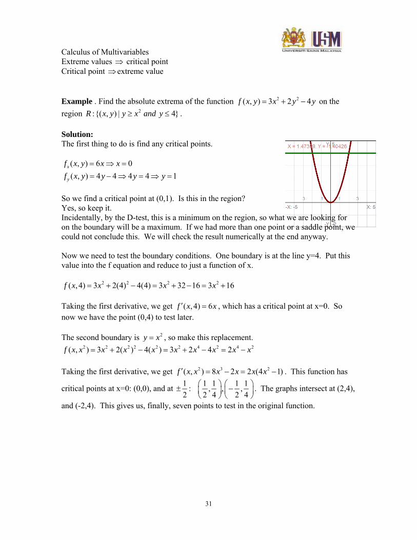
Extreme values ⇒ critical point Critical point ⇒ extreme value Example . Find the absolute extrema of the function 2 2( , ) 3 2 4f x y x y y= + − on the region 2:{( , ) | 4}R x y y x and y≥ ≤ . Solution: The first thing to do is find any critical points.
( , ) 6 0( , ) 4 4 4 4 1
x
y
f x y x xf x y y y y
= ⇒ == − ⇒ = ⇒ =
So we find a critical point at (0,1). Is this in the region? Yes, so keep it. Incidentally, by the D-test, this is a minimum on the region, so what we are looking for on the boundary will be a maximum. If we had more than one point or a saddle point, we could not conclude this. We will check the result numerically at the end anyway. Now we need to test the boundary conditions. One boundary is at the line y=4. Put this value into the f equation and reduce to just a function of x.
2 2 2 2( , 4) 3 2(4) 4(4) 3 32 16 3 16f x x x x= + − = + − = + Taking the first derivative, we get ( , 4) 6f x x′ = , which has a critical point at x=0. So now we have the point (0,4) to test later. The second boundary is 2y x= , so make this replacement.
2 2 2 2 2 2 4 2 4 2( , ) 3 2( ) 4( ) 3 2 4 2f x x x x x x x x x x= + − = + − = − Taking the first derivative, we get 2 3 2( , ) 8 2 2 (4 1)f x x x x x x′ = − = − . This function has
critical points at x=0: (0,0), and at 1 1 1 1 1: , , ,2 2 4 2 4
⎛ ⎞ ⎛ ⎞± −⎜ ⎟ ⎜ ⎟⎝ ⎠ ⎝ ⎠
. The graphs intersect at (2,4),
and (-2,4). This gives us, finally, seven points to test in the original function.
Calculus of Multivariables
32
2 2
2 2
2 2
2 2
(0,1) 3(0) 2(1) 4(1) 2 4 2(0,4) 3(0) 2(4) 4(4) 32 16 16(0,0) 3(0) 2(0) 4(0) 0
1 1 1 1 1 1, 3 2 42 4 2 4 4 8
fff
f
= + − = − = −
= + − = − =
= + − =
⎛ ⎞ ⎛ ⎞ ⎛ ⎞ ⎛ ⎞= + − = −⎜ ⎟ ⎜ ⎟ ⎜ ⎟ ⎜ ⎟⎝ ⎠ ⎝ ⎠ ⎝ ⎠ ⎝ ⎠
2 2
2 2
2 2
1 1 1 1 1 1, 3 2 42 4 2 4 4 8
(2, 4) 3(2) 2(4) 4(4) 12 32 16 28( 2, 4) 3( 2) 2(4) 4(4) 28
f
ff
⎛ ⎞ ⎛ ⎞ ⎛ ⎞ ⎛ ⎞− = − + − = −⎜ ⎟ ⎜ ⎟ ⎜ ⎟ ⎜ ⎟⎝ ⎠ ⎝ ⎠ ⎝ ⎠ ⎝ ⎠
= + − = + − =
− = − + − =
As expected, the minimum on the region at (0,1,-2) is the absolute minimum. And the absolute maximum on the region occurs at the intersections of the boundary conditions, (2,4,28) and (-2,4,28). Since the two values are the same, both are absolute maxima. Lagrange multipliers To find the maximum and minimum values of f(x, y) subject to the constraint g(x, y) = c (assuming these extreme values exist) 1. Find all values of x, y and λ such that ∇f(x, y) = λ∇g(x, y) and g(x, y) = c 2. Evaluate f(x, y) at all of the points found in (1). The largest of these values is the maximum value of f(x, y) and the smallest value is the minimum value of f(x, y). Example : Find the smallest value of x2 + y2 subject to the constraint y + 3x = 3. Solution: Notice that ∇f = 2xi + 2yj and ∇g = 3i + j. Using Lagrange multipliers, we have ∇f = λ∇g, where λis a scalar. This gives us the three equations 2x = 3 λ (1) 2y = λ (2) y + 3x = 3 (3) Solve for x and y in (1) and (2), respectively, we have x = (3/2) λand y = λ /2. Plugging these into (3), we have (λ/2) + 3(3λ/2) = 3 ⇔ 5λ = 3. So λ= 3/5. Plugging in λ= 3/5 into our equations above, we see that x = 9/10 and y = 3/10. Example :
Calculus of Multivariables
33
Find the maximum and minimum values of the function f(x, y) = x2 + 2y2 that lie on the circle x2 + y2 = 1. Solution: Using Lagrange multipliers, we have ∇f = λ∇g, where λis a scalar. This gives us the three equations 2x = 2xλ (1) 4y = 2yλ (2) x2 + y2 = 1 (3) From (1), we have that either x = 0 or λ= 1. If x = 0, then (3) tells us that y = ±1. So, we have the points (0, ±1). If λ= 1, then (2) gives us 4y = 2y, so y = 0. But if y = 0, (3) tells us that x ±1. This gives us the points (±1, 0). Evaluating f(x, y) at these four points, we have f(0, 1) = 2, f(0, –1) = 2, f(1, 0) = 1, and f(–1, 0) = 1. Thus, the maximum value of f(x, y) on the circle x2 + y2 = 1 is f(0, ±1) = 2 and the minimum value is f(±1, 0) = 1. To find the maximum and minimum values of f(x, y) subject to the constraint g(x, y) = c (assuming these extreme values exist)
i. Find all values of x, y and λ such that ∇f(x, y) = λ∇g(x, y) and g(x, y) = c
ii. Evaluate f(x, y) at all of the points found in (1). The largest of these values is the
maximum value of f(x, y) and the smallest value is the minimum value of f(x, y).
Example : Find the smallest value of x2 + y2 subject to the constraint y + 3x = 3. Solution: Notice that ∇f = 2xi + 2yj and ∇g = 3i + j. Using Lagrange multipliers, we have ∇f = λ∇g, where λ is a scalar. This gives us the three equations 2x = 3 λ (1) 2y = λ (2) y + 3x = 3 (3) Solve for x and y in (1) and (2), respectively, we have x = (3/2) λ and y = λ /2. Plugging these into (3), we have (λ/2) + 3(3λ/2) = 3 ⇔ 5λ = 3. So λ= 3/5. Plugging in λ= 3/5 into our equations above, we see that x = 9/10 and y = 3/10. Practice 16: Find the maximum and minimum values of the function f(x, y) = x2 + 2y2 that lie on the circle x2 + y2 = 1. References
Calculus of Multivariables
34
1. Paul Dawkins, (2011) , Paul's Online Math Notes [Online Access: on September 2011 http://tutorial.math.lamar.edu/Classes/CalcIII/3DCoords.aspx ]
2. Dan Clegg,Barbara Frank, ,(2003), Multivariable calculus 5th edition, Brooks/Cole Thomson Learning
Calculus Of Multivariables
1
Double Integral 1. Objectives To compute the volume of a solid bounded by a surface z = f(x, y) and a region in the x-y plane, we can integrate in one direction to find the cross-sectional area of thin slices of the solid, then integrate in the other direction to find the volume of the solid. You should be able to compute the double integral of a function of two variables for various bounded regions in the x-y plane. 2. The antiderivative of functions of 2 variables Let ),( yxf be a function of two variables. The antiderivative of ),( yxf with respect to x is denoted by ∫ dxyxf ),( . Similarly, the antiderivative of ),( yxf with respect to y is denoted
by ∫ dyyxf ),( .
[ ] ),(),( yxfdxyxfx
=∂∂ ∫ and [ ] ),(),( yxfdyyxf
y=
∂∂∫
Example 1 Antiderivative with respect to x Find the antiderivative of 22 332 xyxy ++ with respect to x. Solution
∫ +++=++ )(3)332( 32222 yCxxyyxdxxyxy Example 2 Antiderivative with respect to y Find the antiderivative of 22 yx + with respect to y. Solution
∫ ++=+ )(31)( 3222 xCyyxdyyx
3. The definite integral of functions of 2 variables
Calculus Of Multivariables
2
How to find the definite integral ∫b
a
dyyxf ),( of a function of 2 variables?
In ∫b
a
dyyxf ),( , the limits of integration refer to limits for y.
∫b
a
dyyxf ),( = ),(),( axFbxF − , where ∫= dyyxfyxF ),(),( .
Example 3
Evaluate the definite integral ∫ +1
0 22 )( dyyx .
Solution
1
0
1
0 3222
31)(
=
=∫ ⎥⎦
⎤⎢⎣⎡ +=+
y
yyyxdyyx
= ⎥⎦⎤
⎢⎣⎡ +
312x − [0+0]
= x2 + 31
4. Iterated Integrals 4.1 Successive integrals
dxdyyxfxx
xx
xyy
xyy∫ ∫=
=
=
= ⎥⎦⎤
⎢⎣⎡2
1
2
1
)(
)(),( , obtained by two successive integrations, is called an
iterated integral.
Calculus Of Multivariables
3
Example 4
Evaluate the iterated integral dxdyyx∫ ∫ ⎥⎦⎤
⎢⎣⎡ +
2
1
1
0 22 )(
Solution
dxdyyx∫ ∫ ⎥⎦⎤
⎢⎣⎡ +
2
1
1
0 22 )( = ∫ +
2
1 2 )
31( dxx
= 2
1
3
33 ⎥⎥⎦
⎤
⎢⎢⎣
⎡+
xx
= ⎟⎠⎞
⎜⎝⎛ +−⎟
⎠⎞
⎜⎝⎛ +
31
31
32
38
= 38
4.2 Interchanging the order of integration Example 5
Evaluate the iterated integral dydxyx∫ ∫ ⎥⎦⎤
⎢⎣⎡ +
1
0
2
1 22 )(
Solution
dydxyx∫ ∫ ⎥⎦⎤
⎢⎣⎡ +
1
0
2
1 22 )( = ∫ +
1
0 2 )
37( dyy
= 1
0
3
37
31
⎟⎠⎞
⎜⎝⎛ +y
= ⎟⎠⎞
⎜⎝⎛ +−⎟
⎠⎞
⎜⎝⎛ +
30
30
37
31
= 38
Important result:
dxdyyx∫ ∫ ⎥⎦⎤
⎢⎣⎡ +
2
1
1
0 22 )( and dydxyx∫ ∫ ⎥⎦
⎤⎢⎣⎡ +
1
0
2
1 22 )( have the same value!!
Calculus Of Multivariables
4
4.3 Variable Limits of Integration Example 6
Evaluate the iterated integral ∫ ∫ ⎥⎦⎤
⎢⎣⎡1
0
2 dxxydyx
x
Solution Explanation of the steps
∫ ∫ ⎥⎦⎤
⎢⎣⎡1
0
2 dxxydyx
x= dxxy
xy
xy∫
⎥⎥⎥
⎦
⎤
⎢⎢⎢
⎣
⎡ =
=
1
0 2
221 (find the antiderivative with respect to y)
= dxxx∫
⎥⎥⎦
⎤
⎢⎢⎣
⎡−
1
0
53
22 (substitute the limits of integration)
= ∫ −1
0 53 )(
21 dxxx (find the antiderivative with respect to x)
= 241
5. Concept of double integrals 1.1 Definite integral for functions of a single variable
xsfdxxfn
ii
b
an
Δ= ∑∫=∞→
)(lim)(1
provided that the limit exists.
a bxi−1 si xi x
y=f(x)
f(si)
y
Δx=xi-xi-1
Calculus Of Multivariables
5
5.2 Definite integral for functions of two variables
yxtsfdAyxf j
n
ii
m
jmR
nΔΔ= ∑ ∑∫∫
= =∞→∞→),(limlim),(
1 1 provided that the limit exists.
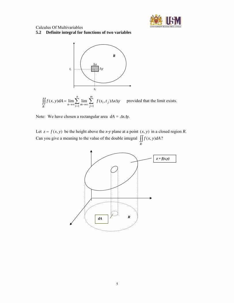
Note: We have chosen a rectangular area dA = ΔxΔy. Let ),( yxfz = be the height above the x-y plane at a point ),( yx in a closed region R. Can you give a meaning to the value of the double integral ∫∫
R
dAyxf ),( ?
R
Δx Δy
si
ti
RdA
z = f(x,y)
Calculus Of Multivariables
6
If ),( yxfz = is equal to the height at ),( yx , then the value of the double integral
∫∫R
dAyxf ),( represents the solid volume over the region R bounded above and below by the
surfaces ),( yxfz = and 0=z (the x-y plane) respectively. 5.3 Some properties of double integrals 1. ∫∫ ∫∫=
R R
dAyxfcdAyxcf ),(),( , where c is a constant.
2. ∫∫ ∫∫ ∫∫+=+
R R R
dAyxgdAyxfdAyxgyxf ),(),()],(),([
3. ∫∫ ∫∫ ∫∫
∪
+=21 1 2
),(),(),(RR R R
dAyxfdAyxfdAyxf if the areas R1 and R2 do not overlap.
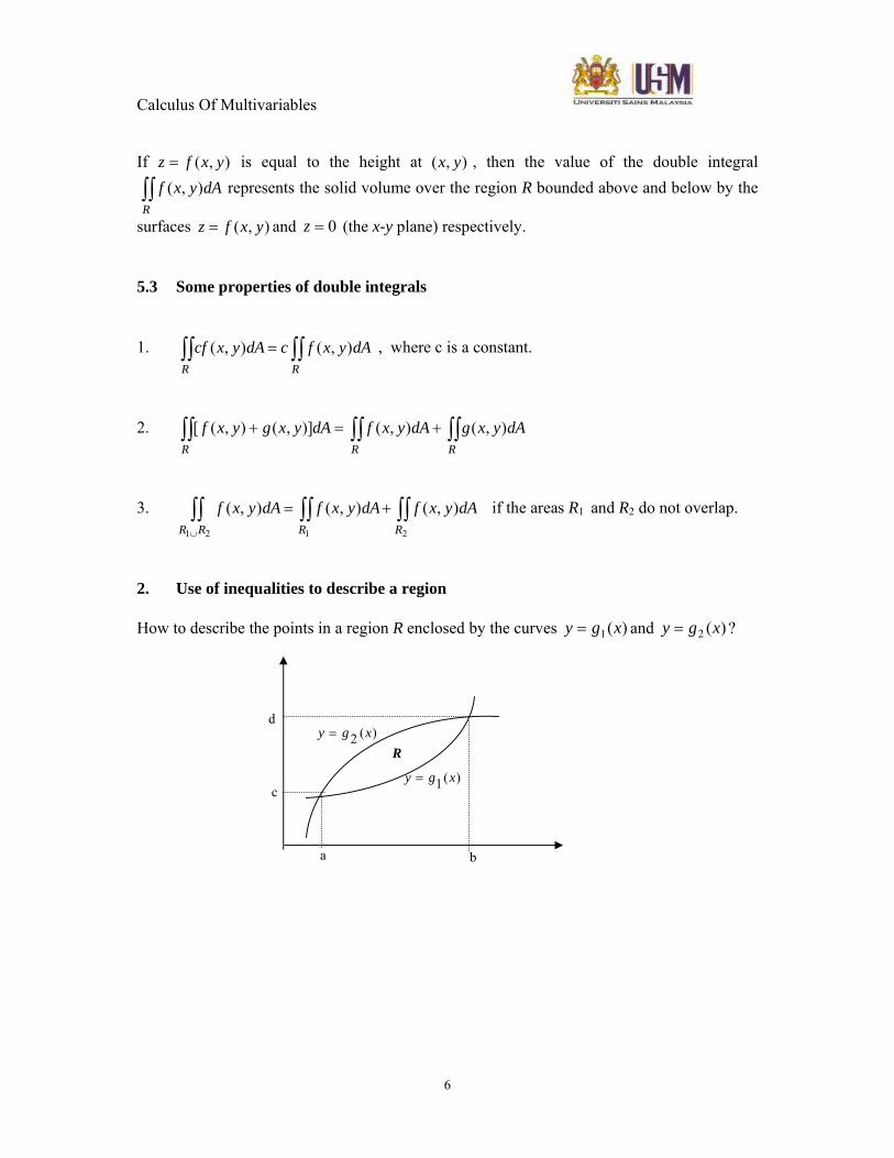
2. Use of inequalities to describe a region How to describe the points in a region R enclosed by the curves )(1 xgy = and )(2 xgy = ?
)(2 xgy =
)(1 xgy =
R
a b
c
d
Calculus Of Multivariables
7
The points (x, y) in R can be described by a set of inequalities: I. g1(x) ≤ y ≤ g2(x) a ≤ x ≤ b or II. g2
−1(y) ≤ x ≤ g1−1(y)
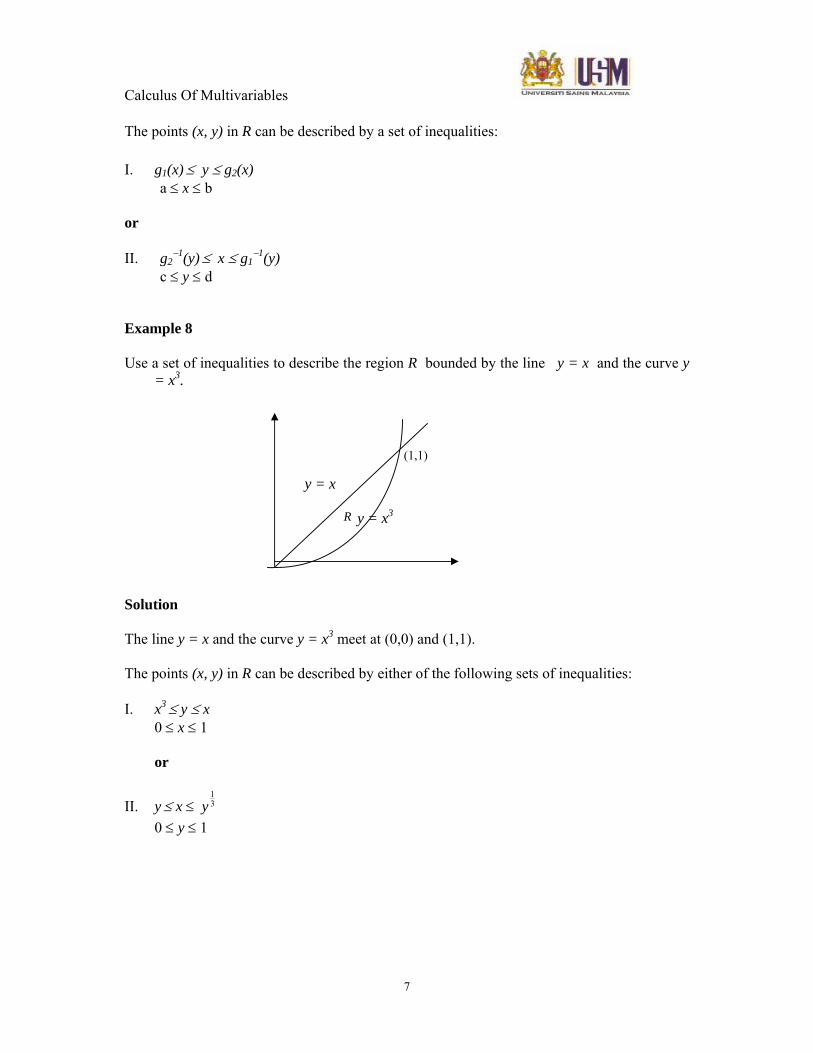
c ≤ y ≤ d Example 8
Use a set of inequalities to describe the region R bounded by the line y = x and the curve y = x3.
y = x y = x3
Solution The line y = x and the curve y = x3 meet at (0,0) and (1,1). The points (x, y) in R can be described by either of the following sets of inequalities: I. x3 ≤ y ≤ x 0 ≤ x ≤ 1 or
II. y ≤ x ≤ 31
y 0 ≤ y ≤ 1
R
(1,1)

Calculus Of Multivariables
8
7. Use of an iterated integral to evaluate a double integral
How to evaluate the double integral ∫∫R
dAyxf ),(?
∫∫R
dAyxf ),( = ∫ ∫ ⎥⎦
⎤⎢⎣⎡b
a
xg
gdxdyyxf
x
)(
2
1 )(),(
= ∫ ∫ ⎥
⎦
⎤⎢⎣
⎡ −
−
d
c
yg
ygdydxyxf
)(
)(
111
2),(
Example 9: By integrating with respect to y first and x second, evaluate the double integral ∫∫
R
xydA ,
where R is the region bounded by the curves y = x and y = x3.
Solution R is the region bounded below and above by g1(x) = x3 and g2(x) = x, and on the left and right by x = 0 and x = 1. g2(x) = x g1(x) = x3
(1,1)
Calculus Of Multivariables
9
∫∫R
xydA = ∫ ∫ ⎥⎦⎤
⎢⎣⎡b
a
xg
gdxdyyxf
x
)(2
1 )(),(
= ∫ ∫ ⎥⎦⎤
⎢⎣⎡1
0
3 dxxydyx
x
= dxxyx
x3
1
0
2
2∫⎥⎥⎦
⎤
⎢⎢⎣
⎡
= dxxx∫ ⎥⎦⎤
⎢⎣⎡ −
1
0 73
21
21
= 161
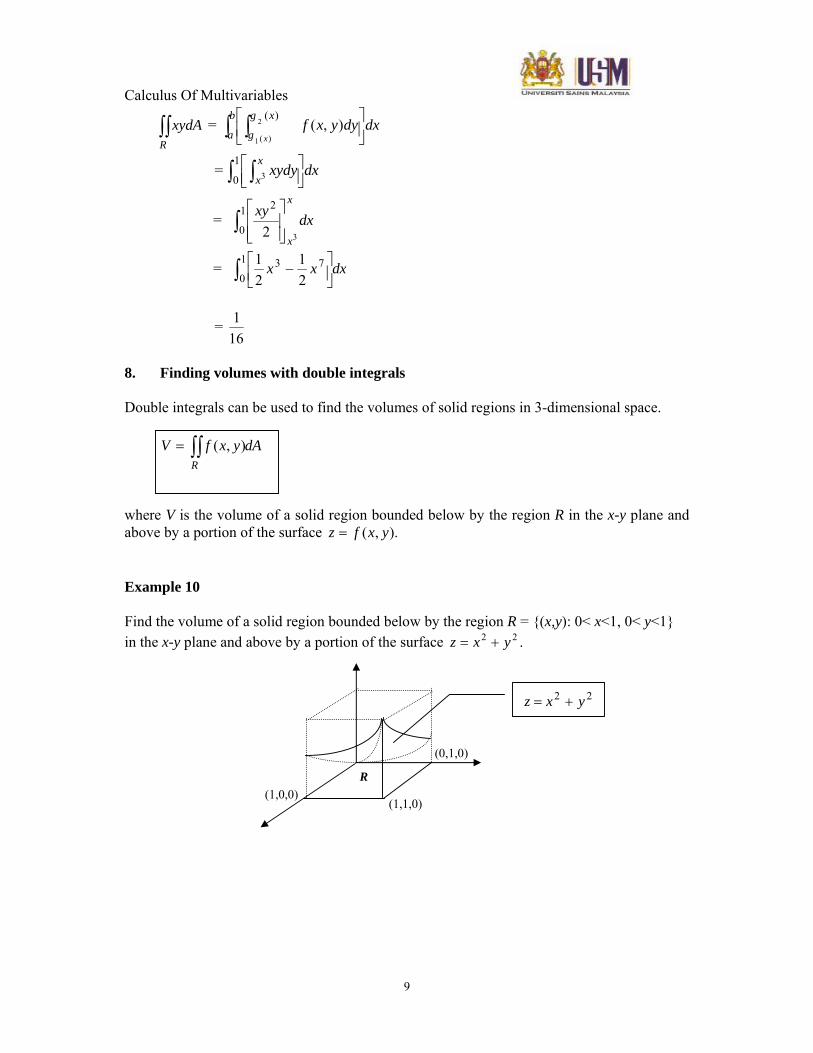
8. Finding volumes with double integrals Double integrals can be used to find the volumes of solid regions in 3-dimensional space. dAyxfV
R∫∫= ),(
where V is the volume of a solid region bounded below by the region R in the x-y plane and above by a portion of the surface ).,( yxfz = Example 10 Find the volume of a solid region bounded below by the region R = {(x,y): 0< x<1, 0< y<1} in the x-y plane and above by a portion of the surface 22 yxz += .
R
(0,1,0)
(1,0,0) (1,1,0)
22 yxz +=
Calculus Of Multivariables
10
Solution
( )
32
31
)(
1
02
1
0
1
022
22
=
⎟⎠⎞
⎜⎝⎛ +=
⎥⎦⎤
⎢⎣⎡ +=
+=
∫
∫ ∫
∫∫
dyy
dydxyx
dAyxVR
9. Other Applications of Double Integrals 9.1 Area The area of a closed region R in the x-y plane is given by A = ∫∫
R
dxdy .
9.2 Mass A thin sheet of material of uniform thickness covers a region R in the x-y plane. Suppose the sheet has varying density ),( yxρ (in kg/m2) at each point (x,y) in the region R. The total mass M of the sheet is given by ∫∫=
R
dxdyyxM ),(ρ .
9.3 Mean value
The mean value of f(x,y) over a closed region R is defined as ∫∫R
dxdyyxfA
),(1 ,
where A is the area of the region R.
R
Calculus Of Multivariables
11
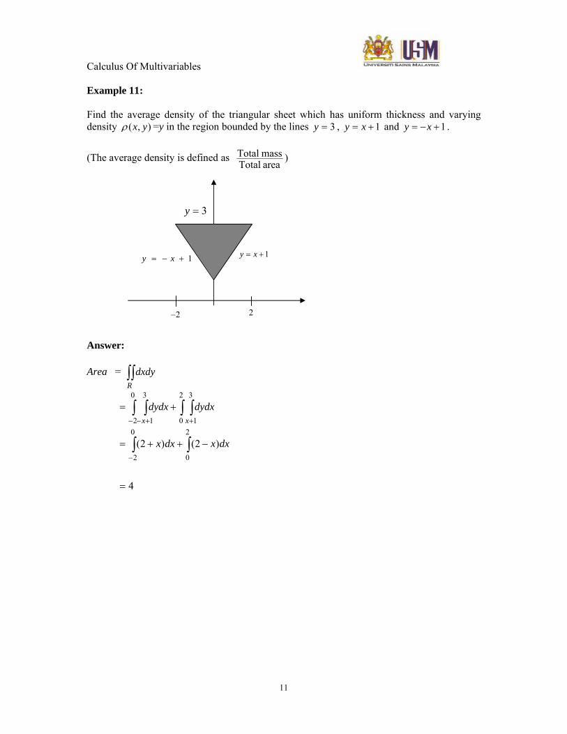
Example 11: Find the average density of the triangular sheet which has uniform thickness and varying density ),( yxρ =y in the region bounded by the lines 3=y , 1+= xy and 1+−= xy . (The average density is defined as
area Totalmass Total )
Answer: Area = ∫∫
R
dxdy
4
)2()2(0
2
2
0
0
2
2
0
3
1
3
1
=
−++=
+=
∫ ∫
∫ ∫ ∫∫
−
− ++−
dxxdxx
dydxdydxxx
3=y
1+= xy1+−= xy
−2 2
Calculus Of Multivariables
12
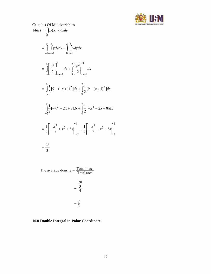
∫∫=R
dxdyyxMass ),(ρ
328
832
1832
1
]82[21]82[
21
])1(9[21])1(9[
21
22
2
0
230
2
23
0
2
2
0
22
0
2
2
0
22
0
2
2
0
3
1
23
1
2
0
2
2
0
3
1
3
1
=
⎥⎥⎦
⎤
⎢⎢⎣
⎡+−−+
⎥⎥⎦
⎤
⎢⎢⎣
⎡++−=
+−−+++−=
+−++−−=
⎥⎥⎦
⎤
⎢⎢⎣
⎡+
⎥⎥⎦
⎤
⎢⎢⎣
⎡=
+=
−
−
−
− ++−
− ++−
∫ ∫
∫ ∫
∫ ∫
∫ ∫ ∫∫
xxxxxx
dxxxdxxx
dxxdxx
dxydxy
ydydxydydx
xx
xx
The average density =
area Totalmass Total
37
4328
=
=
10.0 Double Integral in Polar Coordinate
Calculus Of Multivariables
13
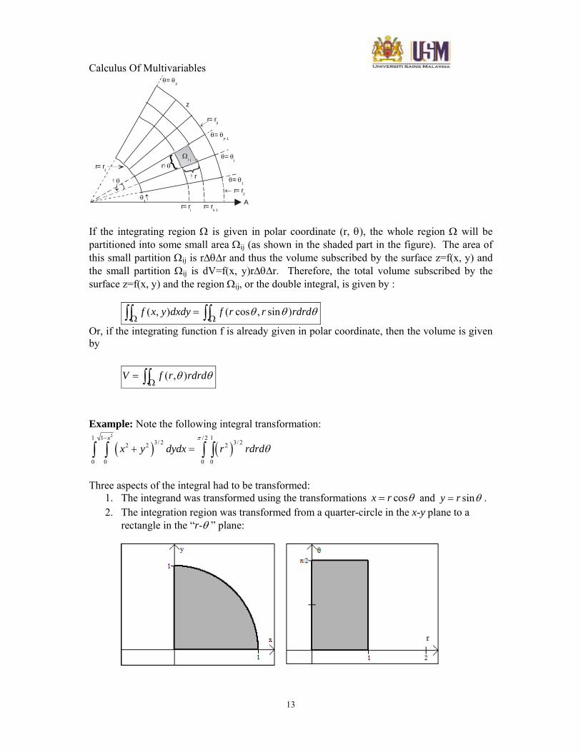
θ θ=2
z
r= r2
θ θ=j+ 1
θ θ=j
θ θ=1
r= r2
r= rj+ 1
r= rj
↑θ1
Ωi j
rr θ{r= r
1
θ↓
A
If the integrating region Ω is given in polar coordinate (r, θ), the whole region Ω will be partitioned into some small area Ωij (as shown in the shaded part in the figure). The area of this small partition Ωij is rΔθΔr and thus the volume subscribed by the surface z=f(x, y) and the small partition Ωij is dV=f(x, y)rΔθΔr. Therefore, the total volume subscribed by the surface z=f(x, y) and the region Ωij, or the double integral, is given by : θθθ rdrdrrfdxdyyxf )sin,cos(),(∫∫ ∫∫Ω Ω
=
Or, if the integrating function f is already given in polar coordinate, then the volume is given by
∫∫Ω= θθ rdrdrfV ),(
Example: Note the following integral transformation:
( ) ( )21 1 / 2 1
3/ 2 3/ 22 2 2
0 0 0 0
x
x y dydx r rdrdπ
θ−
+ =∫ ∫ ∫ ∫
Three aspects of the integral had to be transformed:
1. The integrand was transformed using the transformations cosx r θ= and siny r θ= . 2. The integration region was transformed from a quarter-circle in the x-y plane to a
rectangle in the “r-θ ” plane:
Calculus Of Multivariables
14
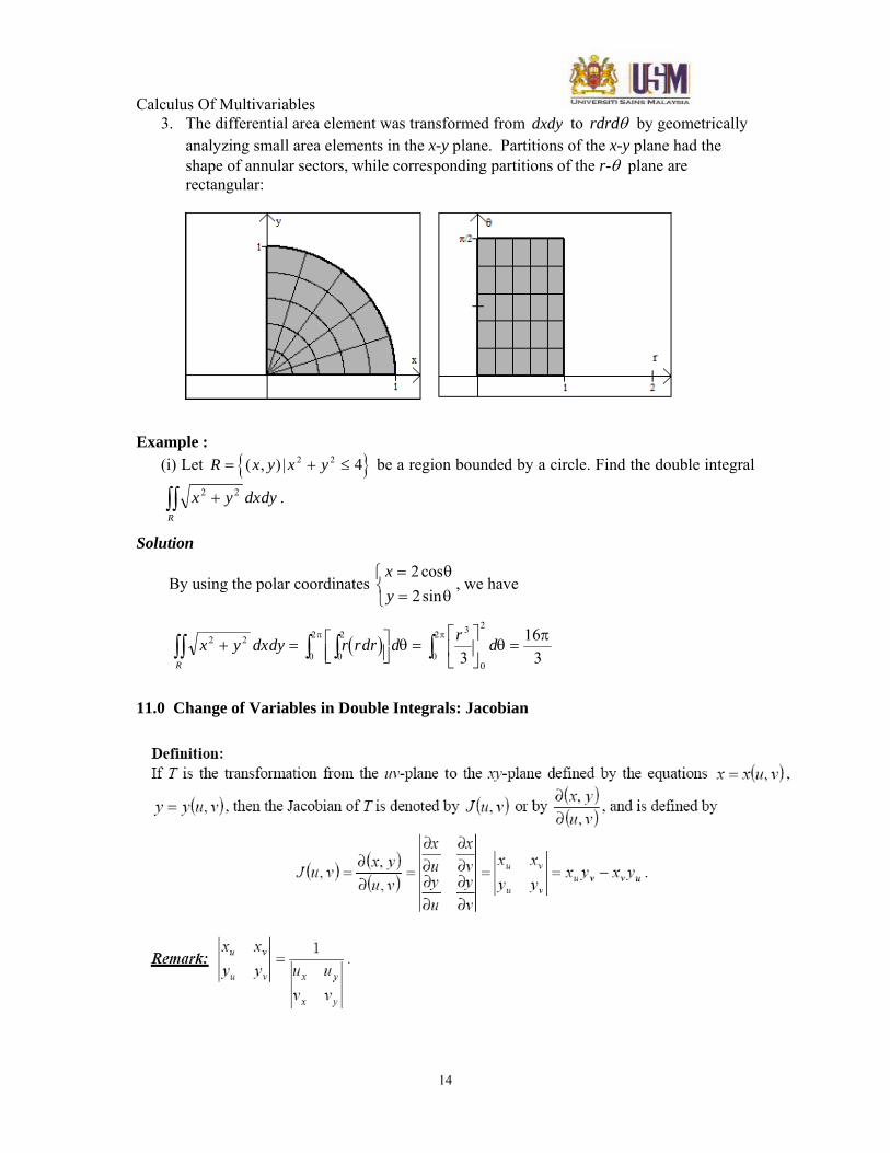
3. The differential area element was transformed from dxdy to rdrdθ by geometrically analyzing small area elements in the x-y plane. Partitions of the x-y plane had the shape of annular sectors, while corresponding partitions of the r-θ plane are rectangular:
Example :
(i) Let { }R x y x y= + ≤( , ) | 2 2 4 be a region bounded by a circle. Find the double integral
x y dxdyR
2 2+∫∫ .
Solution
By using the polar coordinates xy==
⎧⎨⎩
22
cossin
θθ
, we have
( )x y dxdy r rdr d r dR
2 2
0
2
0
2 3
0
2
0
2
316
3+ = ⎡
⎣⎢⎤⎦⎥
=⎡
⎣⎢
⎤
⎦⎥ =∫∫ ∫∫ ∫
π πθ θ
π
11.0 Change of Variables in Double Integrals: Jacobian
Calculus Of Multivariables
15
Theorem: If a region S in the u-v plane is mapped onto the region R in the x-y plane by the one-to-one transformation T defined by ( ),x g u v= and ( ),y h u v= , where g and h have
continuous first derivatives on S, and if f is continuous on R and the Jacobian ( )( )
,,
x yu v
∂∂
is
nonzero on S, then
( ) ( ) ( )( ) ( )( )
,, , , ,
,R S
x yf x y dA f g u v h u v dudv
u v∂
=∂∫∫ ∫∫ .
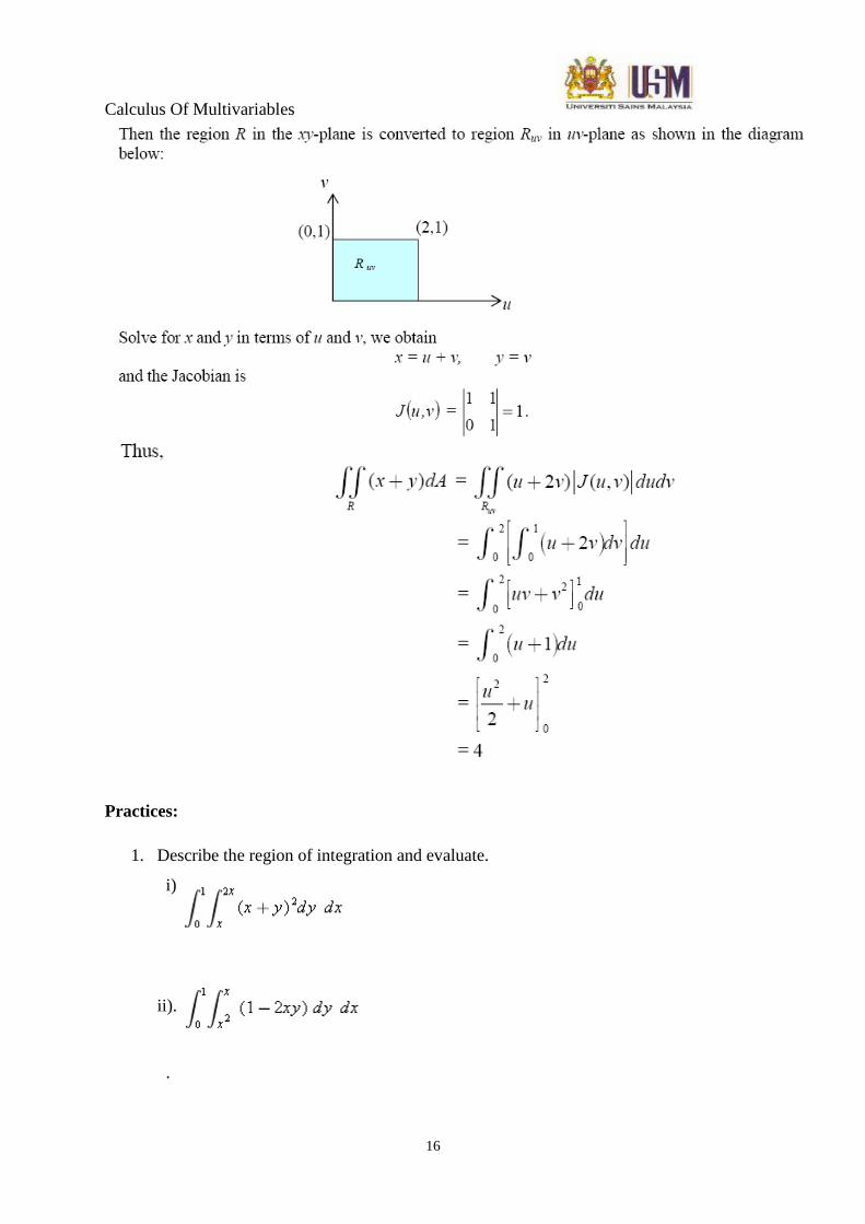
Calculus Of Multivariables
16
Practices:
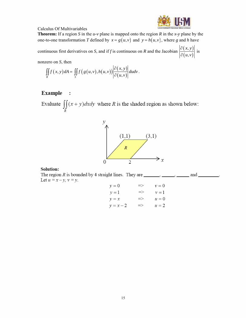
1. Describe the region of integration and evaluate.
i)
ii).
.
Calculus Of Multivariables
17
iii).
iv).
v).
2. Integrate over the triangular region with vertices (0, 0), (1, 1), (1, 2).
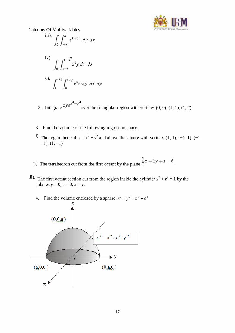
3. Find the volume of the following regions in space.
i) The region beneath z = x2 + y
2 and above the square with vertices (1, 1), (−1, 1), (−1,
−1), (1, −1)
ii) The tetrahedron cut from the first octant by the plane .
iii). The first octant section cut from the region inside the cylinder x2 + z
2 = 1 by the
planes y = 0, z = 0, x = y.
4. Find the volume enclosed by a sphere 2 2 2 2
x y z a
Calculus Of Multivariables
18
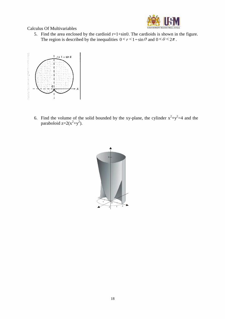
5. Find the area enclosed by the cardioid r=1+sin . The cardioids is shown in the figure.
The region is described by the inequalities 0 1 sin and 0 2r .
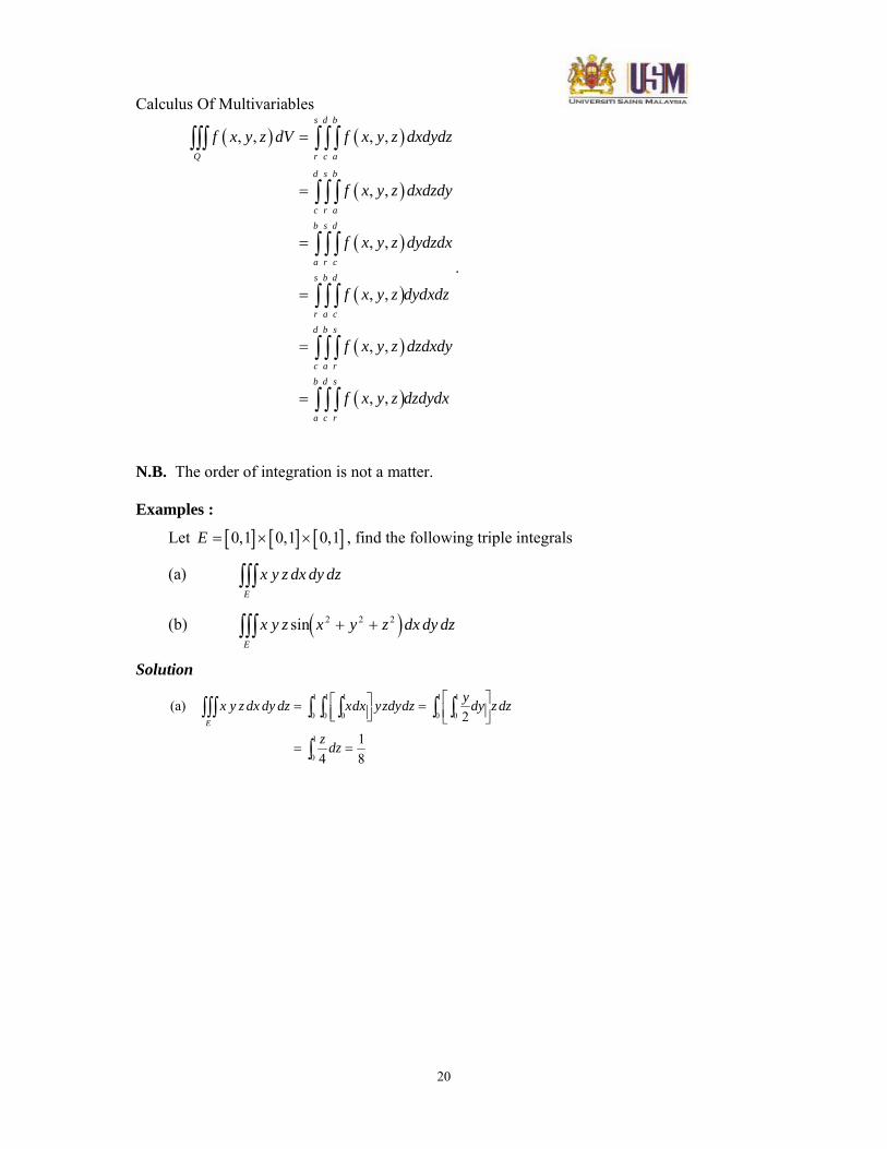
6. Find the volume of the solid bounded by the xy-plane, the cylinder x2+y
2=4 and the
paraboloid z=2(x2+y
2).
-2
-10
221
4

Calculus Of Multivariables
19
Triple integral 1. Objective
A triple integral is an integral taken over a volume of space.You should be able to compute triple integrals.
2. Triple integral
The triple integral is defined with a three variable function f(x, y, z), which is called the integrating function and an integrating region R, which is in the three dimensional space. It should be noted that the function f(x, y, z) cannot be plotted out over a three dimensional domain. In order to define the triple integral, the integrating region R, for example say a parallelepiped as shown in the figure are equally partitioned into small cubics Rijk, which is located at (xi, yj, zk) with lengths of Δx, Δy and Δz in the x, y and z directions respectively. The volume of the small partition Rijk = =ΔxΔyΔz and the triple integral of the function f(x, y, z) over the integrating region R is defined as : ∑∫∫∫∫∫∫ ==
kjiijkkji
RRdVzyxfdVzyxfdxdydzzyxf
,,),,(),,(),,(
2.1 Calculation of triple integral :Order of Integration is Interchangeable If a function f(x, y) is integrable on the box Q = {(x, y, z) | a ≤ x ≤ b, c ≤ y ≤ d, r ≤ z ≤ s }, then we can write the triple integral of f over Q as:
R
Partition Rijk at position of (xi,yj,zk) having vol. of dVijk=ΔxΔyΔz
x
y
z
Calculus Of Multivariables
20
( ) ( )
( )
( )
( )
( )
( )
, , , ,
, ,
, ,
, ,
, ,
, ,
s d b
Q r c a
d s b
c r ab s d
a r c
s b d
r a cd b s
c a rb d s
a c r
f x y z dV f x y z dxdydz
f x y z dxdzdy
f x y z dydzdx
f x y z dydxdz
f x y z dzdxdy
f x y z dzdydx
=
=
=
=
=
=
∫∫∫ ∫ ∫ ∫
∫ ∫ ∫
∫ ∫ ∫
∫ ∫ ∫
∫ ∫ ∫
∫ ∫ ∫
.
N.B. The order of integration is not a matter. Examples :
Let [ ] [ ] [ ]E = × ×0 1 0 1 0 1, , , , find the following triple integrals
(a) x y z dx dy dzE∫∫∫
(b) ( )x y z x y z dx dy dzE
sin 2 2 2+ +∫∫∫
Solution
(a)
x y z dx dy dz xdx yzdydz y dy z dz
z dz
E∫∫∫ ∫∫∫ ∫∫
∫
= ⎡⎣⎢
⎤⎦⎥
= ⎡⎣⎢
⎤⎦⎥
= =
0
1
0
1
0
1
0
1
0
1
0
1
2
418
Calculus Of Multivariables
21
( ) ( )
( )
( ) ( )[ ]
( sin sin
cos
cos cos
b)
x yz x y z dxdydz x x y z dx yzdydz
x y z yzdydz
y z y z ydy zdz
E
2 2 2 2 2 2
0
1
0
1
0
1
2 2 2
0
1
0
1
0
1
2 2 2 2
0
1
0
1
12
12
1
+ + = + +⎡⎣⎢
⎤⎦⎥
= − + +⎡⎣⎢
⎤⎦⎥
= + − + +⎡⎣⎢
⎤⎦⎥
∫∫∫ ∫∫∫
∫∫
∫∫
( ) ( )[ ]( ) ( ) ( )[ ]( ) ( ) ( )[ ]
( )
= + − + +
= + − + −
= − + + + +
= − + −
∫
∫
14
1
14
2 1 2
18
2 1 2
18
3 3 2 3 1 1
2 2 2 2
0
1
0
1
2 2 2
0
1
2 2 2
0
1
sin sin
sin sin sin
cos cos cos
cos cos cos
y z y z zdz
z z z zdz
z z z
2.2 Triple integral with a more general integrating region If Q has the form Q = {(x, y, z) | (x, y) ∈ R (a bounded region in the xy plane) and g1(x, y) ≤ z ≤ g2(x, y)}, then
( ) ( )( )
( )2
1
,
,
, , , ,g x y
Q R g x y
f x y z dV f x y z dzdA=∫∫∫ ∫∫ ∫
Example: Find the volume bounded by the planes 2x+y+z=2, x=0, y=0 and z=0. Solution :We need to find
R
V dxdydz= ∫∫∫ bounded by the above 4 planes
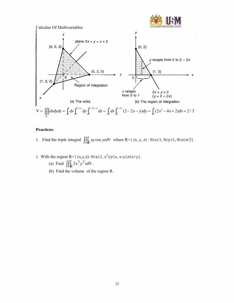
Calculus Of Multivariables
22
1 2 2 2 2 1 2 2 1 2
0 0 0 0 0 0(2 2 ) (2 4 2) 2 / 3
x x y x
R
V dxdydz dx dy dz dx x y dy x x dx− − − −
= = = − − = − + =∫∫∫ ∫ ∫ ∫ ∫ ∫ ∫
Practices: 1. Find the triple integral ∫∫∫R yzdVxy cos where R={ (x, y, z) : 0≤x≤1, 0≤y≤1, 0≤z≤π/2}.
2. With the region R={ (x,y,z): 0≤x≤1, x2≤y≤x, x-y≤z≤x+y}.
(a) Find ∫∫∫R zdVyx 232 .
(b) Find the volume of the region R.


![EDX-F03 EDX-F04 [EUM-E] - valook3d.clvalook3d.cl/fichas/conectividad/dmx_inalambricos/1901.pdf · It is able to store 6 scenes through DMX control panel ECP-103 . It is allowed to](https://img.pdfslide.us/doc/110x75/5b7b5a9e7f8b9a004b8c7da1/edx-f03-edx-f04-eum-e-it-is-able-to-store-6-scenes-through-dmx-control-panel.jpg)


![DX-610 626[EUM-L]](https://img.pdfslide.us/doc/110x75/54079577dab5ca7c508b4761/dx-610-626eum-l.jpg)
