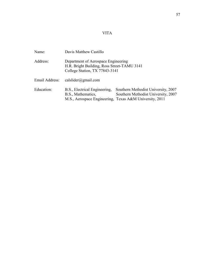
Embed Size (px)
Citation preview

EULER-BERNOULLI IMPLEMENTATION OF SPHERICAL ANEMOMETERS FOR
HIGH WIND SPEED CALCULATIONS VIA STRAIN GAUGES
A Thesis
by
DAVIS MATTHEW CASTILLO
Submitted to the Office of Graduate Studies of
Texas A&M University
in partial fulfillment of the requirements for the degree of
MASTER OF SCIENCE
May 2011
Major Subject: Aerospace Engineering
Euler-Bernoulli Implementation of Spherical Anemometers for High Wind Speed
Calculations via Strain Gauges
Copyright 2011 Davis Matthew Castillo
EULER-BERNOULLI IMPLEMENTATION OF SPHERICAL ANEMOMETERS FOR
HIGH WIND SPEED CALCULATIONS VIA STRAIN GAUGES
A Thesis
by
DAVIS MATTHEW CASTILLO
Submitted to the Office of Graduate Studies of
Texas A&M University
in partial fulfillment of the requirements for the degree of
MASTER OF SCIENCE
Approved by:
Chair of Committee, John E. Hurtado
Committee Members, Shankar Bhattacharyya
Edward B. White
Head of Department, Demitris Lagoudas
May 2011
Major Subject: Aerospace Engineering
iii
ABSTRACT
Euler-Bernoulli Implementation of Spherical Anemometers for High Wind Speed
Calculations via Strain Gauges. (May 2011)
Davis Matthew Castillo, B.S., Southern Methodist University
Chair of Advisory Committee: Dr. John E. Hurtado
New measuring methods continue to be developed in the field of wind
anemometry for various environments subject to low-speed and high-speed flows,
turbulent-present flows, and ideal and non-ideal flows. As a result, anemometry has
taken different avenues for these environments from the traditional cup model to sonar,
hot-wire, and recent developments with sphere anemometers. Several measurement
methods have modeled the air drag force as a quadratic function of the corresponding
wind speed. Furthermore, by incorporating non-drag fluid forces in addition to the main
drag force, a dynamic set of equations of motion for the deflection and strain of a
spherical anemometer’s beam can be derived. By utilizing the equations of motion to
develop a direct relationship to a measurable parameter, such as strain, an approximation
for wind speed based on a measurement is available. These ODE’s for the strain model
can then be used to relate directly the fluid speed (wind) to the strain along the beam’s
length.
The spherical anemometer introduced by the German researcher Holling presents
the opportunity to incorporate the theoretical cantilevered Euler-Bernoulli beam with a

iv
spherical mass tip to develop a deflection and wind relationship driven by cross-area of
the spherical mass and constriction of the shaft or the beam’s bending properties.
The application of Hamilton’s principle and separation of variables to the
Lagrangian Mechanics of an Euler-Bernoulli beam results in the equations of motion for
the deflection of the beam as a second order partial differential equation (PDE). The
boundary conditions of our beam’s motion are influenced by the applied fluid forces of a
relative drag force and the added mass and buoyancy of the sphere. Strain gauges will
provide measurements in a practical but non-intrusive method and thus the concept of a
measuring strain gauge is simulated. Young’s Modulus creates a relationship between
deflection and strain of an Euler-Bernoulli system and thus a strain and wind relation can
be modeled as an ODE.
This theoretical sphere anemometer’s second order ODE allows for analysis of
the linear and non-linear accuracies of the motion of this dynamic system at
conventional high speed conditions.

v
DEDICATION
To my greatest inspirations,
My wife and best friend, Samantha,
My dear parents, Luis and Maria,
And My Lord up above.
vi
ACKNOWLEDGEMENTS
First, I would like to thank my advisor, Dr. John E. Hurtado. His support these
past few years has meant everything to my career. His advice and encouragement have
helped me understand concepts and theories that at times appeared to be of a foreign
language. His patience has not only helped with research but with the struggles of
everyday life. I look forward to using his sound advice now and well into my career.
I would like to thank my committee members, Dr. Shankar Bhattacharyya, and
Dr. Edward White, for their support of my research. Dr. Bhattacharyya your classes in
controls helped challenge me to a better understanding of control theory. I would
especially like to thank Dr. Othon Rediniotis for his help in understanding some basic
concepts of fluid theory, which helped my research immensely. A special thanks to Dr.
Haisler and Karen Knabe for helping me get through the administrative hurdles which I
found myself having to jump over frequently.
I would like to acknowledge the financial support of the Human Diversity
Fellowship and the Aerospace Department. I am also thankful for the research work with
Kane’s Method at NASA JSC with L-3 colleagues Dan Erdberg and Dr. Tushar Gosh.
During my graduate years at Texas A&M University, I give thanks to the
inspiration and support from those closest, including, but not limited to Bryan Castillo,
Roberto Espinosa, Ruby Rodriguez, Juan Enciso, Ian Horbaczewski, Amanda Oleksy,
Martin Ore, and Sharon Morgan. Whether in need for words of wisdom, a friend to
study, a workout partner, or help with tough times you have been there for me.

vii
Thanks to my wife for her numerous sacrifices the past few years. Her
motivation and encouragement have helped me become a better man. Also, thanks to my
wife for the many times she helped edit and review my thesis. Finally, thanks to my
parents for listening and offering support through the hardest of times. Thank you for
believing in me and always being proud. Most importantly, however, thanks to my father
in heaven for the strength and spirit to accomplish another life goal.
viii
NOMENCLATURE
Frequency Coefficient and Harmonic of
c Distance of Strain Gauge from Center of Beam
Added Mass Coefficient
Drag Coefficient
Kroneker Delta Function
Dirac Delta Function
Variation Operator
Spherical Coordinate Unit Vectors
Strain of Beam
Approximate Strain with Measurement Error
E Young’s Modulus
Drag Force from Wind
Buoyancy Force
Added Mass Force
I Second Moment of Inertia of Beam
LHS Left Hand Side Notation
Mass of Sphere
Linear Density of Beam, Density of fluid
Potential Fluid Function
Radius of Sphere, Beam
ix
RHS Right Hand Side Notation
Wind Speed, Wind Acceleration
Estimated Wind Speed
x
TABLE OF CONTENTS
Page
ABSTRACT .............................................................................................................. iii
DEDICATION .......................................................................................................... v
ACKNOWLEDGEMENTS ...................................................................................... vi
NOMENCLATURE .................................................................................................. viii
TABLE OF CONTENTS .......................................................................................... x
LIST OF FIGURES ................................................................................................... xii
CHAPTER
I INTRODUCTION ................................................................................ 1
II BACKGROUND .................................................................................. 5
A. Anemometer Background .......................................................... 5
B. Using Spherical Anemometer .................................................... 6
C. Drag Forces ................................................................................ 7
D. Buoyancy and Added Mass Concepts ....................................... 8
E. Hamilton’s Principle via Lagrange’s Method ............................ 11
III DEVELOPING EQUATIONS OF MOTION FOR SPHERE
ANEMOMETER .................................................................................. 12
A. Spherical Anemometer Proposal ............................................... 12
B. Euler-Bernoulli Beam Derivations ............................................ 13
1. Lagrange’s Method ........................................................ 13
2. Lagrangian for Hybrid Body .......................................... 14
3. Non-Homogenous vs. Homogenous .............................. 18
C. Implementing Fluid Forces ........................................................ 19
1. Applying Buoyancy, Added Mass, and Drag ................. 19
2. Separation of Variables .................................................. 20
3. Equations of Motion for Anemometer ........................... 26
4. From EOM PDE to Strain ODE ..................................... 27
xi
CHAPTER Page
IV CALCULATING WIND SPEED ........................................................ 30
A. Simulation Preparation .............................................................. 30
B. Wind Environment Model ......................................................... 31
C. Euler-Bernoulli Beam Model .................................................... 32
D. Simulations ................................................................................ 34
1. Introducing Strain Gauge Noise Parameters .................. 35
2. Introducing Parameter Perturbation .............................. 37
3. Introducing Average Window Method .......................... 41
4. Introducing Frequency Sampling ................................... 43
5. Recording Data Methods: Real-Time vs. Data Logger .. 45
V DISCUSSION ....................................................................................... 49
A. Full-Bridge Strain Gauge Implementation ................................ 49
B. Water Energy Harvesting .......................................................... 51
C. Modification of Frequency ....................................................... 52
D. Additional Dimension Analysis ................................................ 53
VI CONCLUSION ..................................................................................... 55
REFERENCES .......................................................................................................... 57
VITA ......................................................................................................................... 58
xii
LIST OF FIGURES
FIGURE Page
1 Spherical coordinate diagram for sphere mass ........................................... 9
2 Spherical anemometer diagram .................................................................. 13
3 Strain model according to steady wind oscillations .................................. 35
4 Wind model approximations according to steady state ............................. 36
5 Strain model magnitude ............................................................................. 38
6 Perturbation of .................................................................................... 38
7 Perturbation of beam radius ....................................................................... 39
8 Perturbation of elasticity ............................................................................ 40
9 Perturbation of beam length ....................................................................... 40
10 Perturbation of sphere radius ...................................................................... 41
11 Wind estimate with strain gauge noise of 1%, 5%, 10% ........................... 41
12 Wind estimate average method error.......................................................... 42
13 Wind estimate via frequency sampling ...................................................... 44
14 Wind estimate of running average with sampled frequencies .................... 45
15 Wind estimate with running average method error per frequency ............. 45
16 Wind estimate running average method with data logger .......................... 47
17 Wind estimate with data logger and amplitude of 5 mph .......................... 48
18 Wind estimate with data logger and amplitude of 15 mph ........................ 48
19 Simple wheatstone bridge .......................................................................... 50

1
CHAPTER I
INTRODUCTION
This thesis will focus on the analytical modeling of a hybrid body in a high wind
speed environment and the effect of the induced flow forces in a non-viscous fluid.
Hybrid bodies have not always been used to describe bodies of mass in motion due to
the extra degrees of freedom brought into the analytical calculations as a result. It is
common practice to use rigid bodies in most dynamic calculations to avoid the
nonlinearities that a multi-body system can encounter. Additionally, continuous bodies
can experience sheer stresses and compressions among an indiscrete domain; thus, these
additional nonlinearities will impose a variable force in the multi-body system equation
of motion.
Classical Mechanics is often applied to rigid bodies to model their equations of
motion. These simple systems have the center of mass as the object of interest for the
body’s motion. Aerodynamics however requires precision for every degree of freedom
in the system; consequently, external forces applying sheer stress and compression to a
continuous body are subject to numerous influences per point. Finite element methods
have been used often to deal with the additional degrees of freedom that these complex
bodies of masses entail. However, for our theoretical problem we will approach our
modeling of the continuous body with generalized coordinates. In this thesis we will use
Lagrange’s equations for the continuous beam and rigid sphere mass proposed for the
________
The journal model is IEEE Transactions on Automatic Control.

2
anemometer system.
Current research focused on anemometry has made breakthroughs in new
measurement techniques suited for specific conditions [1]. The hybrid model used by
Holling, via optics, a spherical anemometer is used to calculate highly oscillating wind
speeds to a greater capacity than the traditional cup anemometer design and to a similar
accuracy as that of the hot wire anemometer [2]. As a result this spherical anemometer is
calibrated to react with the given wind environment and then extrapolated for a
differential model.
With the increase of natural disasters, wind environments can take many forms.
Tornadoes and high wind speeds of nature can be catastrophic. Careful analysis by a
record of wind speeds in particular neighborhoods could provide benefits to insurance
companies, meteorology, and even civilians. For this reason a robust method of
providing an anemometer to provide accurate but inexpensive readings could be a tool to
be used in the future. Because wind forces can act in unpredictable ways and wind
anemometer with recording abilities could help determine the wind speeds experiences
at one home versus another within close vicinity.
This experimental model has contributed an innovative way to absorb these
contributing forces and relating the wind speed based on the beam’s deflection. The
experimental work established has as a result brought motivation to develop a full
dynamical analysis of this hybrid model to create the equations of motion for a spherical
anemometer including additional inline fluid forces that may not be included in
traditional approximations.

3
The nonlinearities consist of the concepts of the added mass phenomenon,
buoyancy, and drag forces. Although these wind forces can prove to be minimal in most
low fluid density environments, the dynamical model will prove significance, or lack
thereof, in such a system. The goal of the integration of these fluid influences into this
theoretical model is a robust second order differential system which can output wind
measurement approximations for a given wind model.
Creating this robust dynamical model will require accuracy in the calculation of
the deflection in an experimental setting. The development of an estimated dynamic
model for the wind speed according to the equations of motion will be achieved by
adopting this comprehensive model. The basis for this theory’s development consists of
the theories of separation of variables, Euler- Bernoulli beams, Hamilton’s Principle,
Lagrange’s Equations, and steady state solutions.
The development of these necessary theories will construct the dynamic model to
estimate the wind speed of the given experimental environment. By simulating the
dynamic ODE model for the motion of the spherical anemometer, the system’s response
to varying beam properties and wind conditions can be further analyzed. The steps taken
to achieve this dynamic model are as follows:
1. Develop the distinct nonlinear fluid forces which will affect this hybrid
system.
2. Research the properties of continuous bodies for the beam of this spherical
anemometer.

4
3. Use Hamilton’s principle via Lagrange Method to conjure equations of
motion for the hybrid system.
4. Incorporate the boundary conditions for the given system requirements to
satisfy the beam and sphere’s motion subject to all forces in system.
5. Develop a relationship between the beam’s deflections via EOM into the
corresponding wind speed.
6. Calculate the partial differential equations using separation of variables and
uncoupling methods.
7. Create a relationship between strain and the differential equations of motion.
8. Test the dynamic model of strain for behavior.
9. Reiterate process with simulated measurement error to project strain and
wind speed relationship.
10. Implement data recording method for complete simulation.
Once the methodology is achieved, the model will be applied for a variety of
simulation test cases to verify the accuracy to given wind models.
5
CHAPTER II
BACKGROUND
This chapter will briefly introduce the different ways anemometers measure and
approximate wind speed to assemble distinct and similar qualities to the spherical
anemometer. A further description of the Newtonian physics of the fluid induced forces
affecting the spherical anemometer’s motion will be developed to bond the relationship
between force and motion. For further investigation of the motion of this anemometer
particularly, the beam, an assertion has to be made to define this beam as a continuous
body which thus has infinite number of positions in motion. The development of
kinematics of this hybrid body of mass will be aided by using Hamilton’s Principle and
Lagrange’s Method.
The contributions by Holling and Blevins consist as the central ideas for this model.
The concepts and derivations of the corresponding fluid forces for this model will be
further explained by applying known fluid properties from works by Blevins. The
deflection, motion from the neutral axis, calculated via Lagrange’s Method will then
become important in developing the relationship to the sought after wind speed
approximation in the proceeding chapter.
A. Anemometer Background
The purpose of anemometers when they were first developed was simple; it needed
to find a method to calculate practical wind speeds. The basic model consists of a
6
number of hemispherical cups connected in an array form by rods to a central vertical
shaft. The use of the cup anemometer simply approximates the wind speed by the
number of turns by the cups due to the wind force applied in a specific period of time.
Hot-wire anemometers have also been used for high frequency analysis of rapidly
changing winds found in turbulence wind conditions. Holling’s experiment revealed a
rapidly changing wind environment is best read with a hot-wire anemometer for speed;
however, the sphere anemometer more frequently provides better approximations of the
wind model’s speed without over-speeding like the traditional cup anemometer does in
the same environment. The sphere anemometer demonstrates an improvement from the
over-speeding problem the cup anemometer showed with higher frequency winds [2].
B. Using Spherical Anemometer
Holling’s model proves that the wind induces a drag force to be the main driving
component of the beam’s excitation and motion; for this case, the drag will be a
component to develop and include in the beam model’s equations. Blevins’s contribution
to buoyancy and added mass forces for flow induced models will contribute to the rest of
the force application for this model. The flexibility of this anemometer contributes to the
hybrid aspect of this body mass and thus introduces a different kinematic model with
specific properties. The flexibility in this spherical anemometer can lead to several
uncertainties and degrees of freedom as a result but for the purpose of the wind
conditions and model needed we will assume the Euler Bernoulli Beam properties for
the flexible vertical shaft of this anemometer.

7
C. Drag Forces
Drag has been used in a general basis as a force with quadratic velocity
dependence,
(2-1)
The drag force is best suited to comply at relative high fluid speeds (wind speed
in this case). Ideal flow is assumed to avoid additional considerations such as shear,
viscosity, and other fluid non-linearities. These generalizations are made with the
consideration that the wind speed of the environment is much greater than the speed of
the body mass. However, when considering fluids and masses that accelerate quickly, a
beam with a relative drag force is better suited according to Blevins’s formula [3].
(2-2)
In this linear relative drag force it be must be noted that the measured units
are that of Newtons per length of the cross section. The rest of the variables are familiar
to the traditional drag force such as a varying drag coefficient, (dependent on the
shape of the body mass) in the given fluid with density . When given the scenario
of the anemometer exposed to a wind environment governed as ’s properties, the
drag force is dynamically dependent upon the fluid speed, U, and the speed of the
anemometer, . The motion of the anemometer, y references the deflection from the
beam’s neutral axis, position at complete rest. This beam’s deflection, y, is both a
function of time and position since the deflection of the beam will vary along the beam

8
and with respect to time. The numerous points of motion and deflection will make the
drag force of the anemometer in its entirety complex due to the drag forces subject not
just upon the spherical mass but also along the beam of the anemometer. However if a
spherical mass’s cross sectional area can be relatively large compared to a thin beam’s
cross sectional area; consequently, the drag along the thin beam can be neglected. The
parameter considerations in Chapter 5 will detail the equations used to make the
mentioned assumptions.
D. Buoyancy and Added Mass Concepts
Two additional forces that develop for a mass present in a fluid flow include
buoyancy and added mass. Air is still subject to same inline fluid forces as denser fluids
such as water but air’s significantly lower density lowers the magnitude of these two
forces.
Buoyancy is commonly referred to in examples masses submerged in fluids,
commonly water, to show the fluid force phenomenon opposing other forces such as
gravity. Added Mass is also present in the movements of mass structures submersed in
fluids under fluid acceleration.
Both of these are considered inline forces and a result of the pressure gradient
present at the surface of the mass subject to the wind speed model. This inertial force as
described by Blevins can be calculated by means of the integral equation for

9
(2-3)
Blevins identifies the potential function for the flow over a sphere with radius of
R as:
(2-4)
With the potential function known for the flow surrounding a spherical mass, the
Navier-Stokes equation can be used applying the potential equation’s properties for the
purpose of calculating the pressure along the spherical mass. Under the assumption of an
inviscid fluid the Navier-Stokes equation can be re-written as:
(2-5)
This gradient’s argument can be inferred to equal to a constant in space or a
function of time . Thus Blevins states the pressure as,
(2-6)
The inline force integral requires the normal vector and dS to be calculated.
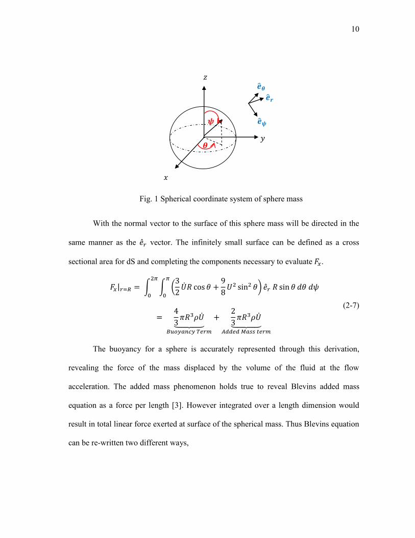
Because the principal mass affected is a sphere, Figure 1 geometrically projects the
simpler evaluation via spherical coordinates.
10
With the normal vector to the surface of this sphere mass will be directed in the
same manner as the vector. The infinitely small surface can be defined as a cross
sectional area for dS and completing the components necessary to evaluate .
(2-7)
The buoyancy for a sphere is accurately represented through this derivation,
revealing the force of the mass displaced by the volume of the fluid at the flow
acceleration. The added mass phenomenon holds true to reveal Blevins added mass
equation as a force per length [3]. However integrated over a length dimension would
result in total linear force exerted at surface of the spherical mass. Thus Blevins equation
can be re-written two different ways,
Fig. 1 Spherical coordinate system of sphere mass
11
(2-8)
By calculating and applying the previous equation it can be calculated to be
composed of the accumulation of these forces result in the net fluid forces applied.
E. Hamilton’s Principle via Lagrange’s Method
Classical kinematics can come to a struggle to define this anemometer’s motion
along the beam length due to the continuous with several degrees of freedom. As another
solution better suited to incorporate a continuous body, Hamilton’s principle will derive
a set of differential equations of motion of the given system using generalized
coordinates. Hamilton’s principle allows for the use of the Lagrangian, the basic
building block for using Lagrange’s Method.
Both theories along with the inline fluid forces present in the wind model will be applied
to the Euler-Bernoulli beam theory in the following chapter.
12
CHAPTER III
DEVELOPING EQUATIONS OF MOTION FOR SPHERE ANEMOMETER
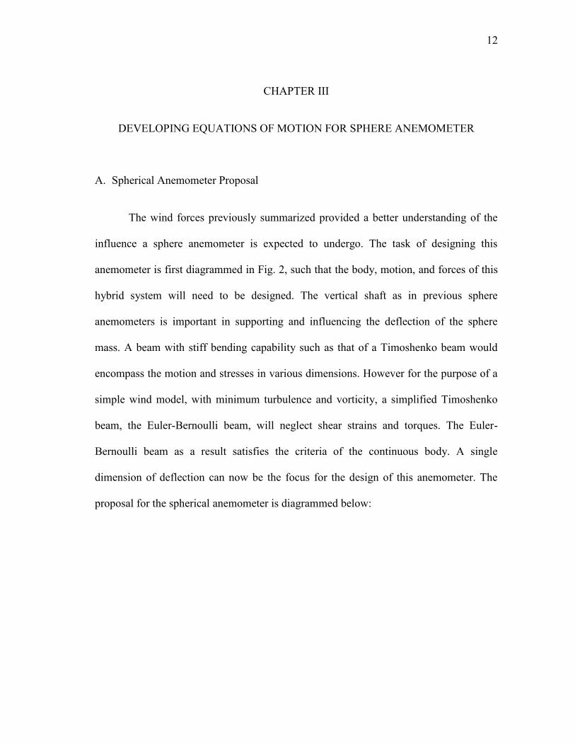
A. Spherical Anemometer Proposal
The wind forces previously summarized provided a better understanding of the
influence a sphere anemometer is expected to undergo. The task of designing this
anemometer is first diagrammed in Fig. 2, such that the body, motion, and forces of this
hybrid system will need to be designed. The vertical shaft as in previous sphere
anemometers is important in supporting and influencing the deflection of the sphere
mass. A beam with stiff bending capability such as that of a Timoshenko beam would
encompass the motion and stresses in various dimensions. However for the purpose of a
simple wind model, with minimum turbulence and vorticity, a simplified Timoshenko
beam, the Euler-Bernoulli beam, will neglect shear strains and torques. The Euler-
Bernoulli beam as a result satisfies the criteria of the continuous body. A single
dimension of deflection can now be the focus for the design of this anemometer. The
proposal for the spherical anemometer is diagrammed below:
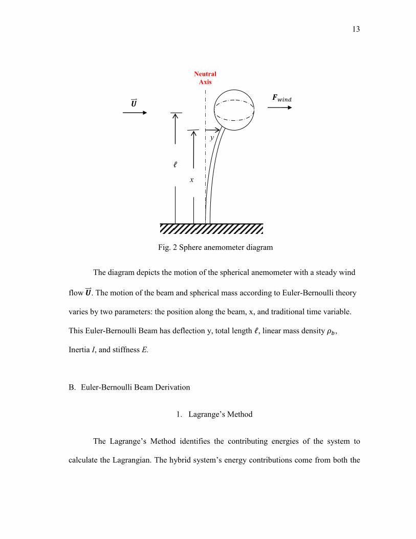
13
The diagram depicts the motion of the spherical anemometer with a steady wind
flow . The motion of the beam and spherical mass according to Euler-Bernoulli theory
varies by two parameters: the position along the beam, x, and traditional time variable.
This Euler-Bernoulli Beam has deflection y, total length , linear mass density ,
Inertia I, and stiffness E.
B. Euler-Bernoulli Beam Derivation
1. Lagrange’s Method
The Lagrange’s Method identifies the contributing energies of the system to
calculate the Lagrangian. The hybrid system’s energy contributions come from both the
Neutral
Axis
x
y
Fig. 2 Sphere anemometer diagram

14
beam and sphere’s kinetic and potential energies. Because of the assumption to use a
cantilevered Euler-Bernoulli beam, torsion influences can be ignored and bending occurs
in a single plane. Thus, deflection along the continuous rigid beam will be parallel to the
wind direction. The motion of the sphere mass moves together with the beam’s end and
thus its speed is equivalent to the beam at the tip. Both the speed of the beam and the
speed of the mass sphere can be identified as and respectively. Therefore
the kinetic energies are:
(3-1)
Similarly, this beam’s potential energy will be composed of the elasticity of
material, second moment of inertia, and deflection along the entirety of the beam. The
spherical mass is a rigid body with a constant potential energy in the deflection of the
beam for small deflections thus only the beam contributes to the dynamic potential
energy, V.
(3-2)
2. Lagrangian for Hybrid Body
The Lagrangian is considered the difference in kinetic minus potential energy;
however, a complete system can be composed of discrete, continuous, and boundary
15
parts. Thus we can develop Hamilton’s Principle further with the full Lagrangian known
as:
(3-3)
In this beam’s case, the complete Lagrangian only has continuous and boundary
components due to the lack of a discrete component in the cantilevered beam system.
The continuous part here corresponds to the kinetic and potential energy along the length
of the beam. The boundary part corresponds with the mass tip’s properties.
As described in the previous section the main wind force will be applied upon the
spherical mass at the beam’s end and thus produce work energy in the anemometer
system. For the development of the following PDE equations, the non-potential
work will influence the energy contributions for the hybrid system and thus the
Lagrangian. The non-potential forces in this system consist of the combination of inline
wind forces. Therefore,
(3-4)
only represents the non-potential forces acting at the length of the beam,
specifically the mass tip. The development of Euler Bernoulli Beams complies with the
Lagrange-D’Alembert Principle, which states the following:
(3-5)

16
The Lagrangian, L, is expressed in terms of a variation by the operator. This
satisfies the equation made possible by Hamilton’s Principle. Thus variation of the
Lagrangian in conjunction with Hamilton’s Principle states:
(3-6)
Because of the hybrid system, the satisfying equation will be applied to the
corresponding parts of the system. A note should be made that there is a distinct
difference in the time derivative used with the kinetic terms and the spatial derivatives
appearance with the potential term.
(3-7)
In Equation 3-7, each kinetic and potential variation term prevent a traditional
integration from being used; consequently, the integration by parts method will be used
to progress the derivation process with either respect to time or length. Hurtado explains
this process as one such that the boundary conditions specifically are produced per
17
implementation of integration by parts to the potential variation term [4]. The first
boundary condition term, BC1, is produced from the first integration’s boundary terms
set to zero and the second boundary condition term, BC2, is a result of the second
integration procedure. Next we show both BC1 and BC2 for further evaluation.
Boundary Conditions for Parameter :
BC1: (3-8)
BC2:
(3-9)
By the definition of a variation such that By following
Figure 2, the first two boundary conditions are set for this cantilevered beam.
BC3 :
BC4:
(3-10)
BC3 and BC 4 infer the fixed end of the beam having zero deflections and zero
slopes respectively at all times. Applying these conditions to the first two boundary
conditions allows for the bending moment and shear moment to be identified as shown
below:
BC1: (3-11)
18
BC2:
As a result Equation 3-7’s integral terms simplify to:
(3-12)
3. Non-Homogenous vs. Homogenous
The homogenous partial differential equations lie in the integral of Equation 3-
12. Along with this PDE, the set of non-homogenous boundary conditions in Equations
3-10 and 3-11 accompany the equations. The shear boundary condition is mostly
affected by the sphere mass at length of the beam and thus is not equal to zero. In order
to apply modal analysis to the PDE’s, the equations are rewritten by use of the Dirac
delta function. The Dirac delta function allows for the third boundary condition to be re-
written such that:
(3-13)
With homogenous boundary conditions,
(3-14)
19
C. Implementing Fluid Forces
1. Applying Buoyancy, Added Mass, and Drag
According to the buoyancy equation our buoyancy force will be,
(3-15)
Considering the anemometer is exposed to wind resistance and air’s fluid
properties, Blevins Added Mass component applies to the deflected beam. The scenario
best fits the added mass phenomenon in an accelerating fluid case. So the added mass
force is,
(3-16)
In both equations, indicates the density of air, V is the volume of the mass tip
sphere exposed to the wind environment, U is the wind speed, and is the mass
acceleration. The third component, which this anemometer will be exposed to, is the
drag force. The drag is calculated in a similar fashion to Blevins’ Galloping and
Fluttering cases for the point mass examples he studies. A relative form of the drag force
is introduced by Blevins to factor large body accelerations,
(3-17)
20
These three force components equate to a total wind force representative
of the force affecting the anemometer’s mass tip in the non-homogenous differential
equations of motion derived beforehand.
(3-18)
2. Separation of Variables
The concept of separation of variables is considered for the case of the Euler-
Bernoulli beam due to the partial differential equations subject to two parameters. The
first assumption made is:
(3-19)
Then the Euler Bernoulli equation where and are
constant beam property values. Substitution leads Equation 3-19 to:
(3-20)
The first step for the separation process involves solving for the spatial
component by division of :
(3-21)
21
By introducing as a constant equal to
, then the variable can be defined as
the harmonic frequency to satisfy the orthogonal function in equation
(3-22)
This procedure yields a function with four orthogonal terms.
(3-23)
If we recall the conditions of our non-homogenous partial differential equations
with homogenous boundary conditions, then we can re-state the boundary conditions in
Equation 3-14 with definition in Equation 3-23.
(3-24)
Equations 3-24 entail not just as unknowns to solve but also the
variable. This is representative of the resonance frequency for the hybrid system.
22
Thus, if can be calculated by a system equations that can be analyzed
individually via the matrix representation of the system of equations [A][C] = [0], where
[A] is a 4x4 coefficient representation of our four equation listed above, [C] =
[ , and [0] is a 4x1 matrix of zeros. Solving this problem requires using the
properties of a determinant to set [A] to be a singular matrix (determinant equals zero) to
satisfy the 4 applied boundary conditions of Equations 3-24. Because is left as an
unknown in the system the following infinite solutions can be produced from the
resulting statement:
(3-25)
While Equation 3-25 reveals solutions for , there are infinite frequencies to
choose from. For the purpose of this work only the first three harmonics or available
frequencies will be included. For future works additional frequencies could be used.
To solve for we can re-write as,
(3-26)
Now we can define or y = via index notation. This
method proves efficient in the uncoupling procedure for a T(t) solution, the expansion
and the calculation of . As stated earlier, the beam’s PDE and wind force are re-
written when applied to Equation 3-13 with the new definition for the loading force:
(3-27)
(3-28)
23
In order to arrive at an ordinary differential equation for T(t) we follow the
following: Multiply by and integrate from for both sides,
(3-29)
In Equation 3-23 was defined as an accumulation of orthogonal
components or eigenfunction expansions in Sin, Cos, Sinh, and Cosh [5]. Thus
according, to Byrne’s definition of orthogonal functions via inner spaces the harmonics
of can be subject to the orthogonal condition [6]. Below we can apply the inner space
product to the spatial function:
(3-30)
Here represents a normalized . For normalization, each individual
harmonic will need to be normalized. For example using the variable to normalize the
first as follows:
(3-31)
24
For simplicity of notation the normalized notation will be withheld from the
following derivation but included in the simulation. Evaluating each term individually
yields the following:
The LHS,
(3-32)
(3-33)
The RHS,
(3-34)
25
The term can be recalled from Equation 3-18 to be a function of
terms, thus by substitution and application of definition of y from
Equation 3-19 the terms become expandable.
Because of the drag force’s use of a relative velocity, the absolute value presents
further complexities towards the simplification of the theoretical derivation of these
equations of motion. Experimentally and for simulation purposes an integrator will
satisfy this condition without a problem. Eliminating the absolute value will be
conditional by
For ,
(3-35)
First, Term simplifies:
(3-36)
Second, term:
(3-37)
Third, term:

26
(3-38)
Fourth, term:
(3-39)
Fifth, term:
(3-40)
Now our PDE equation becomes an ODE for T(t):
(3-41)
3. Equations of Motion for Anemometer
The non-linear ODE that results from the equation above occurs when j =i = k,
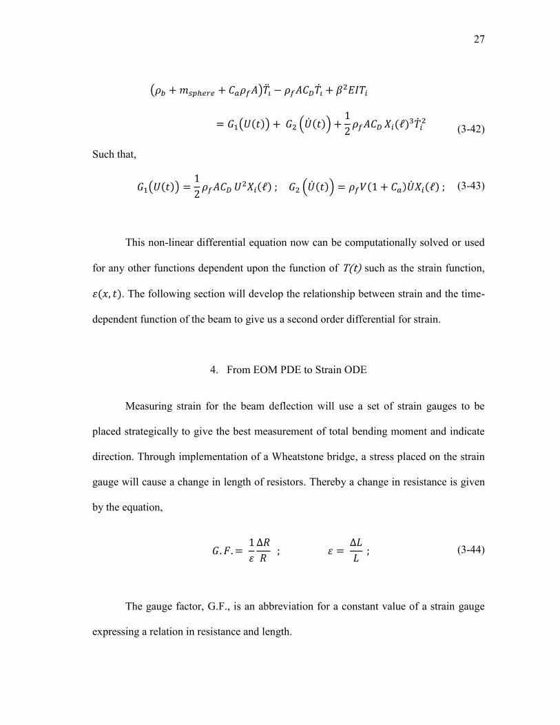
27
(3-42)
Such that,
(3-43)
This non-linear differential equation now can be computationally solved or used
for any other functions dependent upon the function of T(t) such as the strain function,
. The following section will develop the relationship between strain and the time-
dependent function of the beam to give us a second order differential for strain.
4. From EOM PDE to Strain ODE
Measuring strain for the beam deflection will use a set of strain gauges to be
placed strategically to give the best measurement of total bending moment and indicate
direction. Through implementation of a Wheatstone bridge, a stress placed on the strain
gauge will cause a change in length of resistors. Thereby a change in resistance is given
by the equation,
(3-44)
The gauge factor, G.F., is an abbreviation for a constant value of a strain gauge
expressing a relation in resistance and length.
28
According to Young’s Modulus strain is related to stress by,
(3-45)
The function u is the deflection equation for the beam in Equation 3-18 and c is
the displacement of the strain gauge from the central axis of the beam’s center, in this
particular research it will placed on the outside of the beam thus, c will reflect the
magnitude of the beam’s radius.
Thus,
(3-46)
By applying the separation of variable Equation 3-19 to relate between strain and
the equations of motion for anemometer’s beam,
Accordingly we can find , and
(3-47)
We will define
(3-48)
By some algebraic coefficient multiplication we can use to create a second
order differential:
29
(3-49)
This differential equation for the beam’s strain is now a second order non-linear
ODE dependent upon wind speed and acceleration. A computational solution of this
differential can be integrated using MATLAB’s ordinary differential equation solver.
The preceding strain model however contains several parameters that have been briefly
discussed but for the purpose of a future experiment a design method for several
parameters will be detailed in the following chapter. This strain model thus will serve as
the true model for the strain the sphere anemometer will undergo at , the placement of
a test strain gauge. For approximation of wind speed not all the parameters of Equation
3-48 will be available and thus another approximation will be discussed.
30
CHAPTER IV
CALCULATING WIND SPEED
The wind force loads and the derivations of the motion of the sphere anemometer
have led to a strain model that can be used for simulation of the true strain per the theory
implementations. The next phase for the wind speed approximation lays in the design of
both the wind model and the physical anemometer parameter dimensions. As some
theories have been applied earlier the same must be applied in the design of both
environment and system to prepare the simulation.
A. Simulation Preparation
The anemometer simulation will be represented by using the strain model
presented earlier, along with a theoretical strain gauge influenced by white noise to
project realistic measurement errors with accuracy as Omega’s SG-Series strain gauges.
The wind model consists of a ramp function followed by a semi-steady state phase
containing relatively small amplitudes of oscillation. This simulation will undergo a
sixty second run time for the purposes of the following examples. Using the
measurements from the theoretical strain gauge, the steady state equation will
approximate the wind model .
31
B. Wind Environment Model
For the given wind model there will two be two important phases for which the
wind model will pertain to during simulation. These sections can be classified as a
transient or a steady state. The transient state behaves as its name suggests for the initial
ten seconds of the time window. This portion, unlike a steady state, has a fluctuation in
wind speed and acceleration. During the transient phase, the anemometer is subject to all
of the fluid forces previously derived and as a result maintains the complexity of the
complete strain ODE. Although using the complete strain ODE would provide the best
accuracy, an experimental setting would not be able to provide strain rates necessary for
the higher order terms of the model. Because the strain gauge measurement involves
white noise for this simulation, the strain rate cannot be approximated using the rates of
the measurements. Consequently analyzing the steady state approach is the best fitting
for wind approximations.
Thus the following simulations will be analyzed by an environment experiencing
that a ten second wind transient state followed by an semi-ideal steady state experience
with minor oscillations. To assume a steady state we will incorporate the model as
follows:
(4-1)
Where,
32
(4-2)
The purpose of is to simulate the slight oscillations, amplitude , that can
occur during the steadiest phases of a wind environment.
During steady state conditions however the components necessary to
approximate are simply compiled from the measured strain, , without a need for the
measured strain’s rates since constant wind conditions will render , and , negligible to
zero in a perfect constant wind or an ideal steady state.
C. Euler-Bernoulli Beam Model
Several theories and approximations have already been assumed and made for
simplicity purposes in modeling the vertical shaft for the spherical anemometer. The
Euler-Bernoulli beam theory was adopted for this model; as a result, the physical
parameters influenced will be constrained to a degree for the simulations to follow.
In chapter 2, the concept of an Euler-Bernoulli beam was introduced due to the favorable
properties that prevent shear and other trans-axial strains from influencing the primary
deflection of beam from neutral axis. The first constraint distinguishes the material
composition of this beam. The theoretical beam (the experimental anemometer’s shaft)
is restricted to a small deflection to length ratio. A material with a high enough stiffness
and density to prevent large deflections is required. This restriction is defined by Euler-
Bernoulli’s theory which cannot approximate accurately at large deflection ratios due to
the associated non-linear motion. With AL6061’s high density of 2700 kg/m3 and Elastic
33
modulus upwards of 7 Giga-Pascal, the beam should maintain relative small deflections
despite high wind speeds; consequently this aluminum alloy is proposed for testing.
However another essential parameter in an accurate model of an E.B’s beam
deflection pertains to maintaining a 10:1 length to width ratio. As a result, this
assumption for length can be considered for the simulations.
(4-3)
The second approximation to be considered is the negligible drag force of the
beam’s normal surface area to the wind. The general thought is to make sure that the
ratio of drag force upon the spherical mass to the drag force along the beam’s length is
large enough to deem the beam’s length drag force negligible. Thus minimizing the
continuous parameters of the beam’s drag will leave a relatively small load across the
length of the beam. For this reason only a drag force is loaded at the beam’s end. The
parameters to take into account are , , and as the most critical to
affecting the surface area subject to the drag force. Using approximation for the
negligible drag force of
(4-4)
In contrast to the drag force applied at the beam’s end, will
introduce another constraint to consider with design parameters. Ideally a decent
approximation for this condition would suggest
(4-5)
34
Applying Equations 4-3, 4-4, and 4-5 to yields a direct relationship between
the sphere’s radius and the beam’s radius . Equation 4-6 below shows this.
(4-6)
Thus, this leaves the radii of beam and sphere mass variable to a degree of
convenience and practicality. The beam’s width however does need to be large enough
to hold a basic strain gauge such as the SG-Series strain gauges by Omega, featuring a
width ranging from 0.1 - 0.2 inches, depending upon the specific model [6,7].
Incorporating the previous consideration in conjunction with the drag force condition
will allow for the following parameters to be set:
, , and
Although, these parameters are higher larger in magnitude than other previous
experiments, the strain gauge will be physically accommodated under these parameters.
D. Simulations
The simulation of the spherical anemometer is next tested with steady state wind
conditions, variations in beam parameters, error magnitude per strain gauge, parameter
uncertainty, and sampling frequency to accurately compare steady state responses and
the respective wind approximations.
35
1. Introducing Strain Gauge Noise Parameters
The linear relationship between the motion, deflection of the beam, and the strain
active along the beam is directly related by the scaled factor shown previously, thus the
true strain can directly the strain model in Equation 3-49 by ode45’s Rung-Kutta’s
method. In order to understand the effect and magnitude of strain to expect with the
giving considerations our first simulation is the baseline model approximation as shown
below:
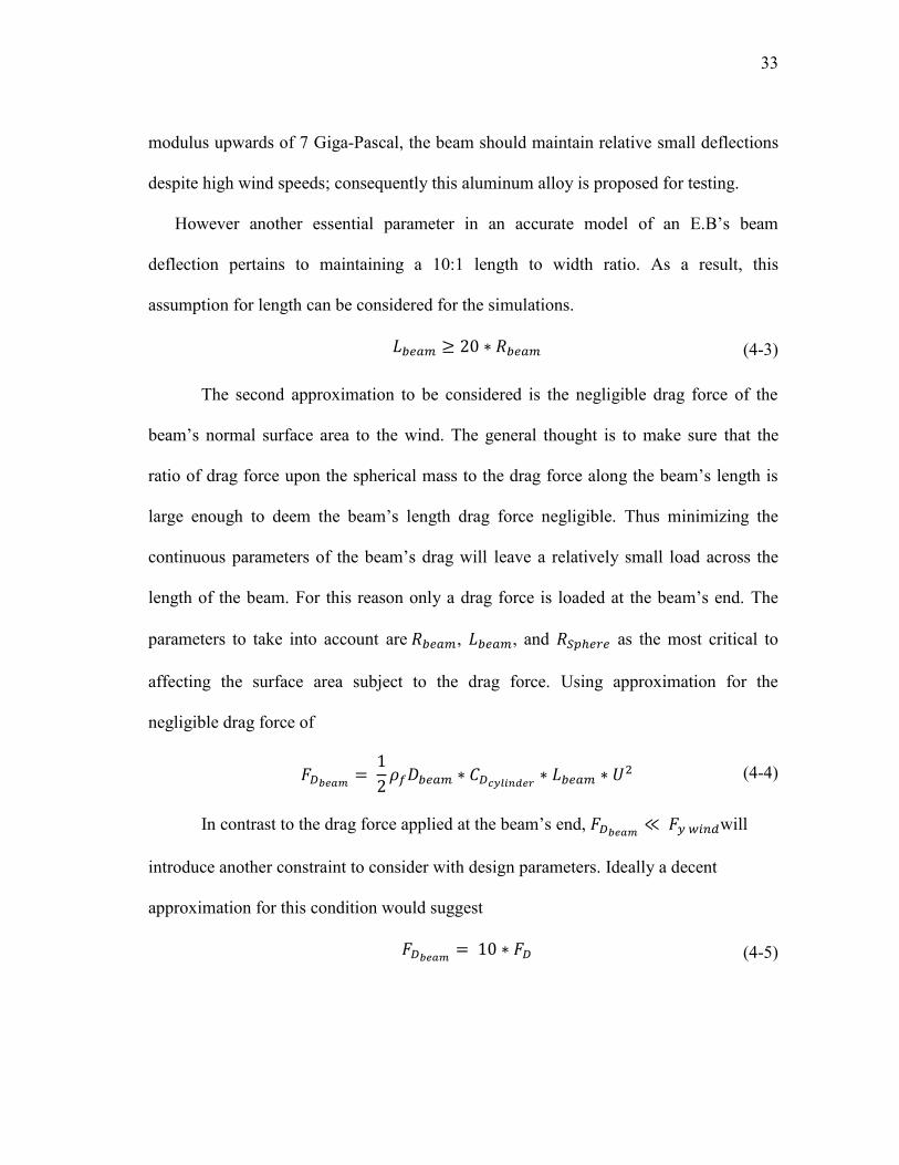
Fig. 3 Strain model according to steady wind oscillation
Figure 3 shows the complete collection of measured strains varied in error
magnitude by a white noise application to the true strain model integrated by ODE45.
Above the true strain model and the measured strains, following the standard deviation
0 10 20 30 40 50 60 -2
0
2
4
6
8
10
12 x 10
-5 Eps & Eps hats Strain
Str
ain
Time (sec)
36
of white noise by 1%, 5%, 10%. True strain, 1% error, 5% error, and 10% error and
shown from thinnest to widest plots respectively.
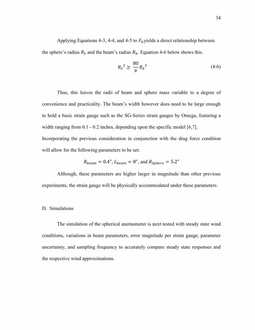
Implementation of the Steady State equation for the approximation of
specifically, is indicated below:
(4-7)
This steady state approximation will allow for wind analysis with varying strain
gauge noise.
Fig. 4 Wind model approximations according to steady state
0 10 20 30 40 50 60 0
20
40
60
80
100
120
140
160
180
200 U
h at with 1%, 5%, 10% std dev error vs. Time
Time (sec)
Speed (
MP
H)
(MP
H)

37
The wind approximations shown in Figure 4 reveal the effects of the strain
gauge’s accuracy. The additional straight line approximately shown at 150 mph is the
calculated by means of an averaged window from t= 30 to 60 seconds. averages
the measured strain during the steady state and thus can calculate a steady state
approximation for the 30 second window span.
These calculations show the constant variance due to the high frequency in the
strain measurements per point due to the non-fixed time steps of the Runge-Kutta
method used. The large number of measurements leaves open the possibility to attempt
averaging a set number of strain measurements and using the corresponding strain
average to continuously update a wind approximation. Using this running average
should help offset the white noise at the expense of a delay depending on the time
window used.
2. Introducing Parameter Perturbation
Known parameters for experimental test can often be inaccurate to a degree due
to numerous reasons such as calibration issues, physical dimension errors, equipment
inaccuracies, etc. Parameter perturbation can be concerning in these simulations as well
if the true strain for the anemometer is not exact due to a slightly longer beam, heavier
density material, or even inaccurate coefficient for drag.
The purpose of the following simulations involves modifying the individual
parameters of the strain steady state equation and observe significant changes if any.
38
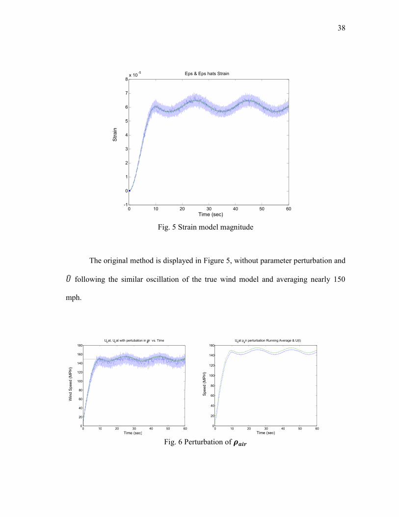
Fig. 5 Strain model magnitude
The original method is displayed in Figure 5, without parameter perturbation and
following the similar oscillation of the true wind model and averaging nearly 150
mph.
Fig. 6 Perturbation of
0 10 20 30 40 50 60 0
20
40
60
80
100
120
140
160 U
h at p a ir perturbation Running Average & U(t)
Time (sec)
Sp
ee
d (
MP
H)
(MP
H)
0 10 20 30 40 50 60 0
20
40
60
80
100
120
140
160
180 U
h at, U h at with pertubation in p
a ir vs. Time
Time (sec)
Win
d S
pe
ed
(M
PH
)
(MP
H)
0 10 20 30 40 50 60 -1
0
1
2
3
4
5
6
7
8 x 10 -5 Eps & Eps hats Strain
Time (sec)
Str
ain
n

39
Figure 6 shows the effects of modifying the density of air, , or distance to
strain from center of beam, having an error of up to 5%, gives a result very similar in
characteristic to the original calculation for . However, the exception in results is a
constant under approximation by 4 mph.
Fig. 7 Perturbation of beam radius
Radius of the beam proves to be one of the most significant and dramatic
changes in wind approximation results. Figure 7 shows how a 5 % error in the beam’s
radius is capable of a -15 mph or -10% errors in wind approximation. Through
perturbation of the beam’s radius it can be inferred that radius length does have at least a
fourth order exponential influence upon the steady state equations.
0 10 20 30 40 50 60 0
20
40
60
80
100
120
140
160
180 U
h at Beam Redius perturbation Running Average & U(t)
Time (sec) 0 10 20 30 40 50 60 0
20 40 60 80
100 120 140 160 180 200
U h at, U
h at with pertubation in Radius of Beam vs. Time
Time (sec)
40
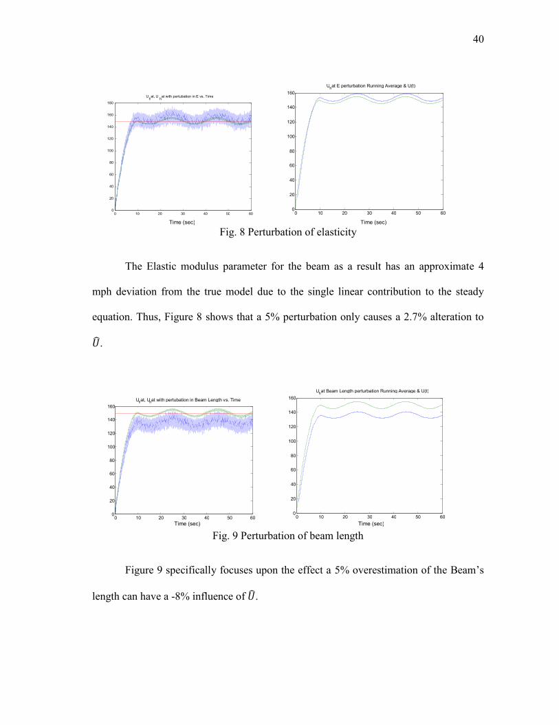
Fig. 8 Perturbation of elasticity
The Elastic modulus parameter for the beam as a result has an approximate 4
mph deviation from the true model due to the single linear contribution to the steady
equation. Thus, Figure 8 shows that a 5% perturbation only causes a 2.7% alteration to
.
Fig. 9 Perturbation of beam length
Figure 9 specifically focuses upon the effect a 5% overestimation of the Beam’s
length can have a -8% influence of .
0 10 20 30 40 50 60 0
20
40
60
80
100
120
140
160 U
h at Beam Length perturbation Running Average & U(t)
Time (sec) 0 10 20 30 40 50 60 0
20
40
60
80
100
120
140
160 U
h at, U h at with pertubation in Beam Length vs. Time
Time (sec)
0 10 20 30 40 50 60 0
20
40
60
80
100
120
140
160 U
h at E perturbation Running Average & U(t)
Time (sec)
0 10 20 30 40 50 60 0 20 40 60 80
100 120 140 160 180
U h at, U
h at with pertubation in E vs. Time
Time (sec)

41
Fig. 10 Perturbation of sphere radius
Figure 10’s slight estimation errors are shown above due to perturbations of
sphere radius.
3. Introducing Average Window Method
Because of the high frequency in MATLAB’s ODEs having a running average
window can take a width of readings and average for a rolling time span which in
effect will average the strain gauges white noise that can interfere with estimating
accuracy of . Shown below in Figure 11 the imminent difference is shown:
Fig. 11 Wind estimate with strain gauge noise 1%, 5%, 10%
0 10 20 30 40 50 60 0
20
40
60
80
100
120
140
160 U
h at Running Average & U(t)
Time (sec)
0 10 20 30 40 50 60 0 20 40 60 80
100 120 140 160 180 200
U h at with 1%, 5%, 10% std dev error vs. Time
Time (sec)
0 10 20 30 40 50 60 0
20
40
60
80
100
120
140
160 U
h at Sphere Radius perturbation Running Average & U(t)
Time (sec) 0 10 20 30 40 50 60 0
20
40
60
80
100
120
140
160
180 U
h at, U h at with pertubation in Radius Sphere vs. Time
Time (sec)
42
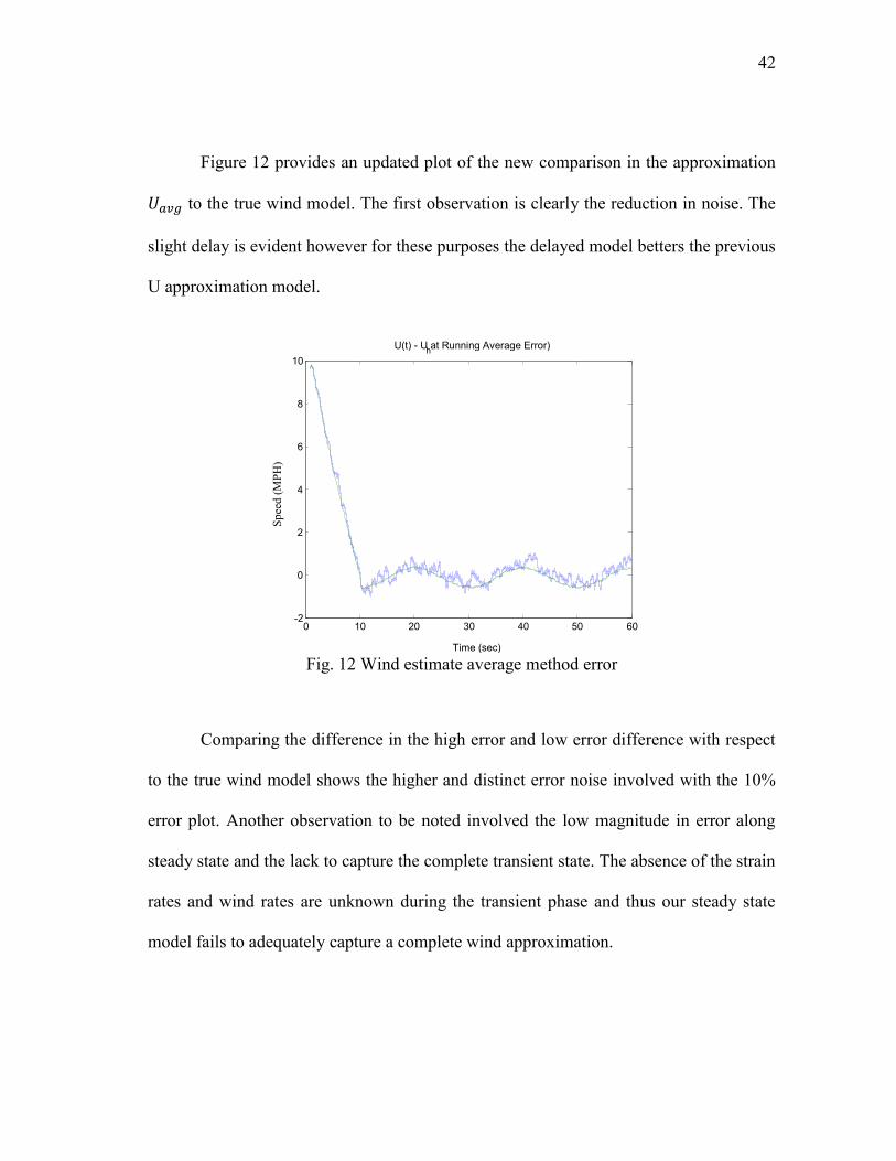
Figure 12 provides an updated plot of the new comparison in the approximation
to the true wind model. The first observation is clearly the reduction in noise. The
slight delay is evident however for these purposes the delayed model betters the previous
U approximation model.
Fig. 12 Wind estimate average method error
Comparing the difference in the high error and low error difference with respect
to the true wind model shows the higher and distinct error noise involved with the 10%
error plot. Another observation to be noted involved the low magnitude in error along
steady state and the lack to capture the complete transient state. The absence of the strain
rates and wind rates are unknown during the transient phase and thus our steady state
model fails to adequately capture a complete wind approximation.
0 10 20 30 40 50 60 -2
0
2
4
6
8
10 U(t) - U
h at Running Average Error)
Time (sec)
Sp
eed
(M
PH
)
(MP
H)
43
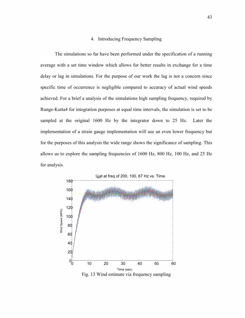
4. Introducing Frequency Sampling
The simulations so far have been performed under the specification of a running
average with a set time window which allows for better results in exchange for a time
delay or lag in simulations. For the purpose of our work the lag is not a concern since
specific time of occurrence is negligible compared to accuracy of actual wind speeds
achieved. For a brief a analysis of the simulations high sampling frequency, required by
Runge-Kutta4 for integration purposes at equal time intervals, the simulation is set to be
sampled at the original 1600 Hz by the integrator down to 25 Hz. Later the
implementation of a strain gauge implementation will use an even lower frequency but
for the purposes of this analysis the wide range shows the significance of sampling. This
allows us to explore the sampling frequencies of 1600 Hz, 800 Hz, 100 Hz, and 25 Hz
for analysis.
Fig. 13 Wind estimate via frequency sampling
0 10 20 30 40 50 60 0
20
40
60
80
100
120
140
160
180 U h at at freq of 200, 100, 67 Hz vs. Time
Time (sec)
Win
d S
pee
d (
MP
H)
(MP
H)
44
The U approximations in Figure 13 tend to indicate the lower frequencies to be
closer to the U(t) model; however, the high fluctuation in all of the sampled
approximation models impedes an accurate conclusion. The wide range of +/- 10 mph
does not provide with a reliable result to infer from. For this reason the running average
is performed upon each sampled model:
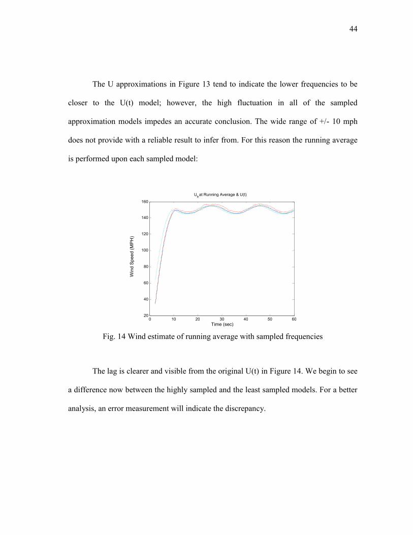
Fig. 14 Wind estimate of running average with sampled frequencies
The lag is clearer and visible from the original U(t) in Figure 14. We begin to see
a difference now between the highly sampled and the least sampled models. For a better
analysis, an error measurement will indicate the discrepancy.
0 10 20 30 40 50 60 20
40
60
80
100
120
140
160 U
h at Running Average & U(t)
Time (sec)
Win
d S
pee
d (
MP
H)
(MP
H)
45
Fig. 15 Wind estimate with running average method error per frequency
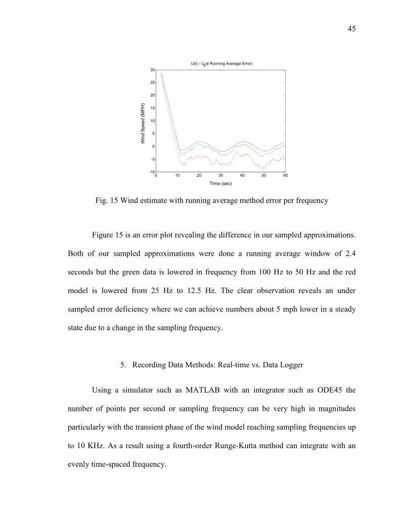
Figure 15 is an error plot revealing the difference in our sampled approximations.
Both of our sampled approximations were done a running average window of 2.4
seconds but the green data is lowered in frequency from 100 Hz to 50 Hz and the red
model is lowered from 25 Hz to 12.5 Hz. The clear observation reveals an under
sampled error deficiency where we can achieve numbers about 5 mph lower in a steady
state due to a change in the sampling frequency.
5. Recording Data Methods: Real-time vs. Data Logger
Using a simulator such as MATLAB with an integrator such as ODE45 the
number of points per second or sampling frequency can be very high in magnitudes
particularly with the transient phase of the wind model reaching sampling frequencies up
to 10 KHz. As a result using a fourth-order Runge-Kutta method can integrate with an
evenly time-spaced frequency.
0 10 20 30 40 50 60 -10
-5
0
5
10
15
20
25
30 U(t) - U
h at Running Average Error)
Time (sec)
Win
d S
pee
d (
MP
H)
(MP
H)
46
For an experimental setting the sampling frequency will be influenced by
memory available for data storage and processing speeds of equipment. Unless working
with real-time equipment or experimental equipment nearby, data loggers provide the
best solution to have data stored to be retrieved at a later time. Utilizing equipment such
as data loggers will require a sampling frequency no higher than 1 Hz. For this reason,
the effect of frequency sampling will be examined for the wind approximation of the
given wind models.
For the following cases a comparison between a 1000 Hz sampled approximation
to a sampled approximation of the theoretical data logger under varying amplitudes in
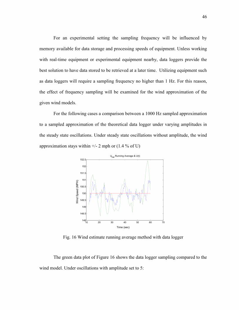
the steady state oscillations. Under steady state oscillations without amplitude, the wind
approximation stays within +/- 2 mph or (1.4 % of U)
Fig. 16 Wind estimate running average method with data logger
The green data plot of Figure 16 shows the data logger sampling compared to the
wind model. Under oscillations with amplitude set to 5:
10 20 30 40 50 60 70 148
148.5
149
149.5
150
150.5
151
151.5
152
152.5 U
hat Running Average & U(t)
Time (sec)
Win
d S
pee
d (
MP
H)
(MP
H)
47
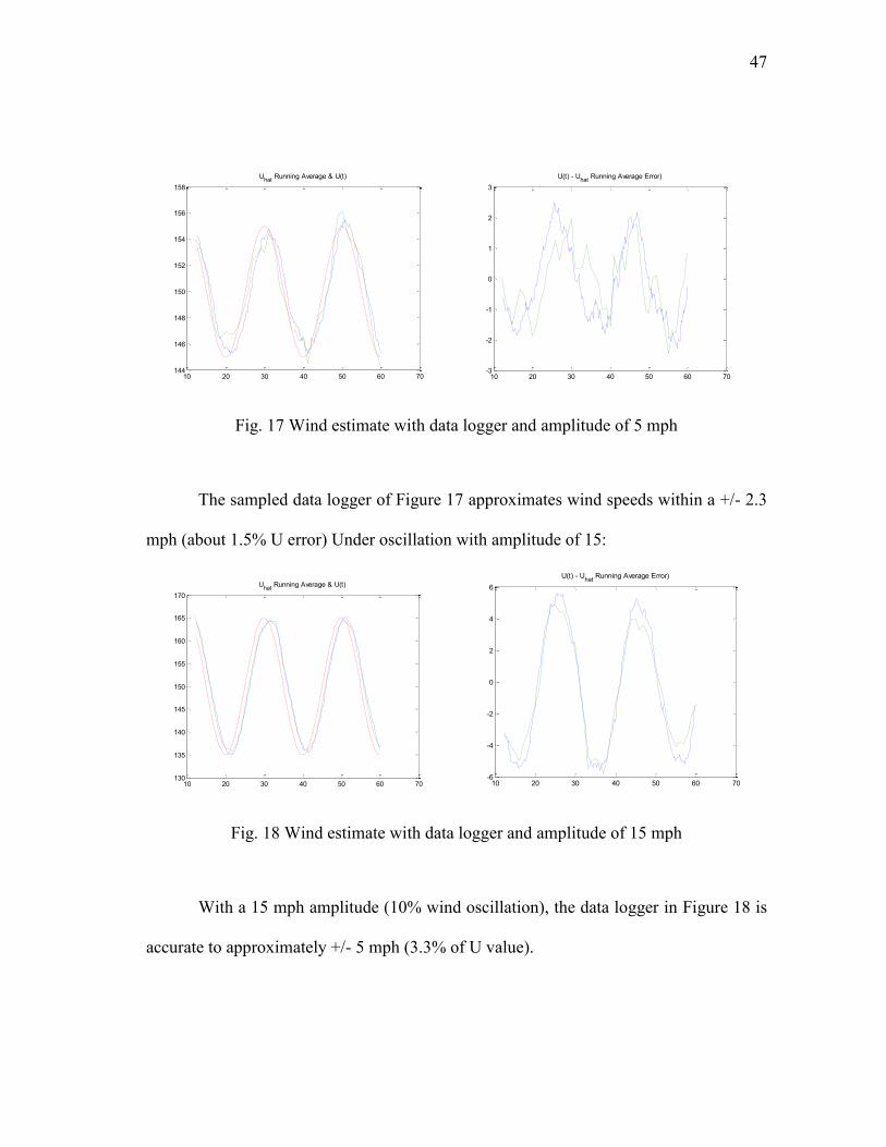
Fig. 17 Wind estimate with data logger and amplitude of 5 mph
The sampled data logger of Figure 17 approximates wind speeds within a +/- 2.3
mph (about 1.5% U error) Under oscillation with amplitude of 15:
Fig. 18 Wind estimate with data logger and amplitude of 15 mph
With a 15 mph amplitude (10% wind oscillation), the data logger in Figure 18 is
accurate to approximately +/- 5 mph (3.3% of U value).
10 20 30 40 50 60 70144
146
148
150
152
154
156
158
Uhat
Running Average & U(t)
10 20 30 40 50 60 70-3
-2
-1
0
1
2
3
U(t) - Uhat
Running Average Error)
10 20 30 40 50 60 70130
135
140
145
150
155
160
165
170
Uhat
Running Average & U(t)
10 20 30 40 50 60 70-6
-4
-2
0
2
4
6
U(t) - Uhat
Running Average Error)
48
CHAPTER V
DISCUSSION
Simulation performances by the steady state strain model for high speed wind
were approximately analyzed for accuracy. Sampling frequency, steady state wind
model, averaging window method and parameter perturbation was tested in Chapter 4.
Strain measurements are designed by following the characteristics of a white noise
subject to a standard derivation of a magnitude high enough to ensure satisfying the
standard tolerances of Omega’s strain gauge specifications [7].
A. Full-Bridge Strain Gauge Implementation
Chapter 4 showed how measurement error was applied due to strain error which
was estimated by a white noise with a tolerance between 1-5%.
National Instruments details the important resistance change and thereby strain by the
schematic implementation of a Wheatstone bridge with simply one main resistor
representing a strain gauge up to all four active resistors representing four strain gauges.
This difference represents a quarter-bridge strain gauge model and the full-bridge strain
gauge respectively.
49
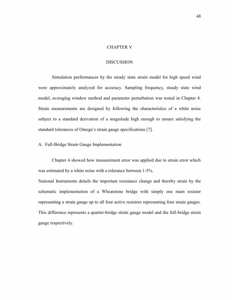
Fig. 19 Simple wheatstone bridge [6]
In Figure 19, the external voltage yields no output voltage if
.
(5-1)
However with stain gauge application in conjunction with Equation 3-43 will
yield variable resistance for . According to a National Instruments’ tutorial,
(5-2)
Here will refer to the nominal resistance per strain gauge, GF is the constant
Gauge Factor, and the compressed or tensed strain [7].
To have a better understanding of exactly how the strain may be calculated in an
experimental setting, we carry out the following example for a full-bridge strain gauge
realization.
For an experimental hardware setup the four strain gauges must be arranged for
compression and tension purposes along the same position of the beam. Each strain
gauge will have a nominal resistance and be accurate within +/- 0.5% according to
50
Agilent [8]. From an experimental setting the of each strain gauge are assumed equal
and thus,
(5-3)
The is the only measurable variable thus,
(5-4)
This is the ideal case though where nominal resistance does not influence the
strain reading. However the tolerance in nominal resistance can influence the actual
strain of the Wheatstone bridge. Thus a statistical analysis could be implemented to
simulated true strains and voltages to establish nominal resistance values not exactly
equal and see how accurately the strain can still be represented by the output voltage
function. Because the full strain gauge contains noise in the resistance but are combined
in the voltage calculations, the noise should reduce with the higher number of
combinations of strains in a compression/tension pair. This simulation would lead the
ground work for typical voltages to look for and anticipate if tested in a wind tunnel with
real time data analysis.
51
B. Water Energy Harvesting
Another growing purpose for investigation involves the use of waves and natural
currents to create and store a clean and renewable energy source. Keeping track and
optimizing the use of the water’s natural to store energy would require a method of
keeping track of the current’s speed. A type of fluid anemometer is necessary in this case
to keep track of the fluids changing speed.
To implement this idea several factors could play into effect such as the
performance needs of such a fluid measuring device. Assuming the purpose is to provide
a simple reading of water speed in a fairly steady environment; the spherical
anemometer is submerged in water but could be designed in a similar fashion to the
anemometer for wind. The fluid density is the top change in this environment from
relatively small 1.8 kg/m3 to magnitude of approximately 990 kg/m
3. One of the things
to consider is how dynamic the water currents will be in terms of sudden currents
changing from steady state. With the application of the running average method, the
way the readings are recorded and the time lag will change to better fit the needs.
Analyzing typical wave speeds will reveal a higher undergoing strain per fluid speed but
overall lower fluid speeds in this scenario.
C. Modification of Frequency
Different weather services describe gusts of wind to be a distinctly higher wind
speed held over a short time span of a few seconds. Thus the approximation model could

52
be expanded to accept steady wind models with oscillations spanning different lengths of
time. An alteration in the frequency of gusts in an otherwise steady wind model could be
analyzed for accuracy by data logger, as done in chapter 4, to see if the calculations are
delayed. The calculations would still involve some approximations as with earlier
examples. Because the recording frequency is approximately 1 Hz and gusts of wind are
at least strong for a couple of seconds, oversampling is not a concern.
One other concern that may need to addressed when the environment model
begins to diverge from the steady state model with not only higher oscillations but
varying frequencies. For example a wind gust will not likely oscillate with the same
period and strength in a normal environment. Thus wind gust could vary from very low
frequencies to gusts of up to 3 seconds and maybe shorter. This could propose a need to
make the model of the anemometer’s resonance frequency is set to be much higher than
that of the wind. Thus changing the physical properties would need to be optimized to
increase frequency. One frequency factor is dependent upon the mass of the mass tip.
However making the mass smaller would also reduce drag and other fluid forces. For
this reason simulations with a hollow sphere could expand the opportunity to introduce
wind gusts and continue broadening the capabilities of this anemometer.
D. Additional Dimension Analysis
Ideal flow was treated to a one dimensional constraint for simplicity but when
experiencing realistic unknown wind direction and conditions, the sphere anemometer is
subject to bending in a combination of directions.
53
A proposed solution would involve expanding the idea of half-bridge Wheatstone
strain gauges. By placing at least two sets of Wheatstone Half-Bridges at the four
quadrants of the sphere anemometer’s beam at least two strain gauges will always be
subject to tension and two to compression. The only exceptions would occur if the wind
direction of is directly perpendicular to a quadrant of the beam. For this case, an
overall strain would have to be calculated by a vector-like combination of both strain
gauge magnitudes.
54
CHAPTER VI
CONCLUSION
The approximation model of this research has provided a viable solution to
implement a sphere anemometer under steady high wind speeds with modest accuracy.
Although many linearized forces and assumptions were made for the purpose of an
attainable ODE to integrate and test different setups; the accuracy of the strain model
proved to be accurate with the filtering effect of an average time window for the wind
speed approximation .
The continued accuracy of the steady strain model proves to be better than
expected despite large amplitude oscillation in wind environment. Parameter
perturbation proved to be critical for the three physical parameter fit to satisfy the
considerations of the anemometer design. The thickness of the beam of this Euler-
Bernoulli revealed the strongest influence for the wind approximation by a great
magnitude.
This approximation algorithm has incorporated a complete dynamic model that
sometimes captures small but still contributing fluid forces. These forces are typically
not incorporated into a sphere anemometer’s algebraic deflection-wind speed model. The
effects of the inline fluid terms can be expected to have a much more significant effect in
a fluid with high density like water. Several possibilities as discussed in the previous
chapter are available to continue pursuing results.
55
A Full-Bridge Wheatstone implementation would statistically reduce the strain
measurement error and thus provide an increased accuracy in the wind approximations.
Implementing a different restriction for the averaging time window due memory
constraints could also affect the delay of the results and/or the accuracy to capture higher
frequency wind model changes by the steady strain model.
Lastly the steady strain model has been dynamically modeled to incorporate the
loads affecting sphere anemometer other than the drag of the mass sphere. By
incorporating D’Alembert’s Principle, Lagrange’s Method, Euler-Bernoulli Beams,
Navier-Stokes theory, and Young’s Modulus the relationship to wind progressed into
complete differential equations of motion.
56
REFERENCES
[1] B. Pedersen, T. Pedersen, H. Klung, N. Van Der Borg, N. Kelley, J. Dahlberg, Wind
speed measurement and use of cup anemometry. In: Hunter, R.S. (Ed.), Expert
Group Study on Recommended Particles for Wind Turbine Testing and Evaluation,
vol. 11, second ed. International Energy Agency, 2003.
[2] M. Holling, B. Schulte, S. Barth, and J. Peinke, “Sphere Anemometer- A Faster
Alternative Solution to Cup Anemometry,” Journal of Physics: Conference Series
vol. 75 no. 1, pp 1-6, 2007.
[3] R. Blevins, Flow-Induced Vibrations. New York, New York: Van Nostrand
Reinhold, 1990, chapter 2.1-2.2, 6.1.
[4] J. Hurtado, Kinematic and Kinetic Principles. College Station, Texas: Lulu
Marketplace, 2007.
[5] S. Han, H. Benaroya, and T. Wei, “Dynamics of Transversely Vibrating Beams
Using Four Engineering Theories,” Journal of Sound and Vibrations, Vol. 225, no.
5, pp. 935 – 988, 1999.
[6] C. L. Byrne, “Selected Topics in Applied Mathematics” in Lecture Notes: University
of Massachusetts Lowell, 2011, pp. 257-262,
http://faculty.uml.edu/cbyrne/amread.pdf
[7] National Instruments, Strain Gauge Measurement, Application Note 078, Austin,
Texas, National Instruments Corporation, 1998.
[8] Agilent Technologies, Practical Strain Gauge Measurements, Application Note 290,
Santa Clara, California, Agilent Technologies, 1999.
57
VITA
Name: Davis Matthew Castillo
Address: Department of Aerospace Engineering
H.R. Bright Building, Ross Street-TAMU 3141
College Station, TX 77843-3141
Email Address: [email protected]
Education: B.S., Electrical Engineering, Southern Methodist University, 2007
B.S., Mathematics, Southern Methodist University, 2007
M.S., Aerospace Engineering, Texas A&M University, 2011


![An isogeometric collocation approach for Bernoulli–Euler ... · the so-called differential quadrature methods [51–54]. A particular feature of Bernoulli–Euler beam and Kirchhoff](https://img.pdfslide.us/doc/110x75/602c9703becf5e244842da2c/an-isogeometric-collocation-approach-for-bernoulliaeuler-the-so-called-differential.jpg)