Ettore Majorana: Unpublished Research Notes on Theoretical Physics

Fundamental Theories of Physics

An International Book Series on The Fundamental Theories of Physics:Their Clarification, Development and Application

Series Editors:GIANCARLO GHIRARDI, University of Trieste, ItalyVESSELIN PETKOV, Concordia University, CanadaTONY SUDBERY, University of York, UKALWYN VAN DER MERWE, University of Denver, CO, USA

Volume 159

For other titles published in this series, go to www.springer.com/series/6001

Ettore Majorana:Unpublished Research Noteson Theoretical Physics

Edited by

S. Esposito

University of Naples “Federico II”Italy

E. Recami

University of BergamoItaly

A. van der Merwe

University of DenverColorado, USA

R. Battiston

University of PerugiaItaly

EditorsSalvatore Esposito Alwyn van der MerweUniversità di Napoli “Federico II” University of DenverDipartimento di Scienze Fisiche Department of Physics and AstronomyComplesso Universitario di Monte S. Angelo Denver, CO 80208Via Cinthia USA80126 NapoliItaly

Erasmo Recami Roberto BattistonUniversità di Bergamo Università di PerugiaFacoltà di Ingegneria Dipartimento di Fisica24044 Dalmine (BG) Via A. PascoliItaly 06123 Perugia

Italy

Back cover photo of E. Majorana: Copyright by E. Recami & M. Majorana, reproduction of the photo isnot allowed (without written permission of the right holders)

ISBN 978-1-4020-9113-1 e-ISBN 978-1-4020-9114-8

Library of Congress Control Number: 2008935622

c© 2009 Springer Science + Business Media B.V.No part of this work may be reproduced, stored in a retrieval system, or transmitted in any form or by anymeans, electronic, mechanical, photocopying, microfilming, recording or otherwise, without the writtenpermission from the Publisher, with the exception of any material supplied specifically for the purpose ofbeing entered and executed on a computer system, for the exclusive use by the purchaser of the work.

Printed on acid-free paper

9 8 7 6 5 4 3 2 1

springer.com

“But, then, there are geniuses like Galileo and Newton.Well, Ettore Majorana was one of them...”

Enrico Fermi (1938)

CONTENTS

Preface xiii

Bibliography xxxvii

Table of contents of the complete set of Majorana’s Quaderni(ca. 1927-1933) xliii

CONTENTS OF THE SELECTED MATERIAL

Part I

Dirac Theory 3

1.1 Vibrating string [Q02p038] 31.2 A semiclassical theory for the electron [Q02p039] 4

1.2.1 Relativistic dynamics 41.2.2 Field equations 7

1.3 Quantization of the Dirac field [Q01p133] 221.4 Interacting Dirac fields [Q02p137] 25

1.4.1 Dirac equation 251.4.2 Maxwell equations 271.4.3 Maxwell-Dirac theory 291.4.3.1 Normal mode decomposition 311.4.3.2 Particular representations of Dirac operators 32

1.5 Symmetrization [Q02p146] 351.6 Preliminaries for a Dirac equation in real terms [Q13p003] 35

1.6.1 First formalism 361.6.2 Second formalism 381.6.3 Angular momentum 401.6.4 Plane-wave expansion 441.6.5 Real fields 451.6.6 Interaction with an electromagnetic field 45

vii

viii E. MAJORANA: RESEARCH NOTES ON THEORETICAL PHYSICS

1.7 Dirac-like equations for particles with spin higher than 1/2[Q04p154] 471.7.1 Spin-1/2 particles (4-component spinors) 471.7.2 Spin-7/2 particles (16-component spinors) 481.7.3 Spin-1 particles (6-component spinors) 481.7.4 5-component spinors 55

Quantum Electrodynamics 57

2.1 Basic lagrangian and hamiltonian formalism for the electro-magnetic field [Q01p066] 57

2.2 Analogy between the electromagnetic field and the Dirac field[Q02a101] 59

2.3 Electromagnetic field: plane wave operators [Q01p068] 642.3.1 Dirac formalism 68

2.4 Quantization of the electromagnetic field [Q03p061] 712.5 Continuation I: angular momentum [Q03p155] 782.6 Continuation II: including the matter fields [Q03p067] 822.7 Quantum dynamics of electrons interacting with an electro-

magnetic field [Q02p102] 842.8 Continuation [Q02p037] 942.9 Quantized radiation field [Q17p129b] 952.10 Wave equation of light quanta [Q17p142] 1002.11 Continuation [Q17p151] 1012.12 Free electron scattering [Q17p133] 1042.13 Bound electron scattering [Q17p142] 1122.14 Retarded fields [Q05p065] 116

2.14.1 Time delay 1182.15 Magnetic charges [Q03p163] 119

Appendix: Potential experienced by an electric charge [Q02p101] 121

Part II

Atomic Physics 125

3.1 Ground state energy of a two-electron atom [Q12p058] 1253.1.1 Perturbation method 1253.1.2 Variational method 1283.1.2.1 First case 1293.1.2.2 Second case 1303.1.2.3 Third case 131

3.2 Wavefunctions of a two-electron atom [Q17p152] 1333.3 Continuation: wavefunctions for the helium atom [Q05p156] 1363.4 Self-consistent field in two-electron atoms [Q16p100] 1413.5 2s terms for two-electron atoms [Q16p157b] 1443.6 Energy levels for two-electron atoms [Q07p004] 144

3.6.1 Preliminaries for the X and Y terms 148

CONTENTS ix

3.6.2 Simple terms 1513.6.3 Electrostatic energy of the 2s2p term 1553.6.4 Perturbation theory for s terms 1573.6.5 2s2p 3P term 1583.6.6 X term 1593.6.7 2s2s 1S and 2p2p 1S terms 1693.6.8 1s1s term 1703.6.9 1s2s term 1743.6.10 Continuation 1753.6.11 Other terms 176

3.7 Ground state of three-electron atoms [Q16p157a] 1833.8 Ground state of the lithium atom [Q16p098] 184

3.8.1 Electrostatic potential 1843.8.2 Ground state 185

3.9 Asymptotic behavior for the s terms in alkali [Q16p158] 1903.9.1 First method 1913.9.2 Second method 195

3.10 Atomic eigenfunctions I [Q02p130] 1973.11 Atomic eigenfunctions II [Q17p161] 2013.12 Atomic energy tables [Q06p026] 2043.13 Polarization forces in alkalies [Q16p049] 2053.14 Complex spectra and hyperfine structures [Q05p051] 2113.15 Calculations about complex spectra [Q05p131] 2193.16 Resonance between a p (� = 1) electron and an electron with

azimuthal quantum number �′ [Q07p117] 2233.16.1 Resonance between a d electron and a p shell I 2243.16.2 Eigenfunctions of d 5

2, d 3

2, p 3

2and p 1

2electrons 225

3.16.3 Resonance between a d electron and a p shell II 2273.17 Magnetic moment and diamagnetic susceptibility for a one-

electron atom (relativistic calculation) [Q17p036] 2293.18 Theory of incomplete P ′ triplets [Q07p061] 233

3.18.1 Spin-orbit couplings and energy levels 2333.18.2 Spectral lines for Mg and Zn 2373.18.3 Spectral lines for Zn, Cd and Hg 238

3.19 Hyperfine structure: relativistic Rydberg corrections [Q04p143] 2393.20 Non-relativistic approximation of Dirac equation for a two-

particle system [Q04p149] 2423.20.1 Non-relativistic decomposition 2433.20.2 Electromagnetic interaction between two charged par-

ticles 2443.20.3 Radial equations 245

3.21 Hyperfine structures and magnetic moments: formulae and ta-bles [Q04p165] 246

3.22 Hyperfine structures and magnetic moments: calculations[Q04p169] 2513.22.1 First method 2513.22.2 Second method 254

x E. MAJORANA: RESEARCH NOTES ON THEORETICAL PHYSICS

Molecular Physics 261

4.1 The helium molecule [Q16p001] 2614.1.1 The equation for σ-electrons in elliptic coordinates 2614.1.2 Evaluation of P2 for s-electrons: relation between W

and λ 2634.1.3 Evaluation of P1 275

4.2 Vibration modes in molecules [Q06p031] 2754.2.1 The acetylene molecule 278

4.3 Reduction of a three-fermion to a two-particle system [Q03p176] 282

Statistical Mechanics 287

5.1 Degenerate gas [Q17p097] 2875.2 Pauli paramagnetism [Q18p157] 2885.3 Ferromagnetism [Q08p014] 2895.4 Ferromagnetism: applications [Q08p046] 3005.5 Again on ferromagnetism [Q06p008] 307

Part III

The Theory of Scattering 311

6.1 Scattering from a potential well [Q06p015] 3116.2 Simple perturbation method [Q06p024] 3166.3 The Dirac method [Q01p106] 317

6.3.1 Coulomb field 3186.4 The Born method [Q01p109] 3196.5 Coulomb scattering [Q01p010] 3216.6 Quasi coulombian scattering of particles [Q01p001] 324

6.6.1 Method of the particular solutions 3276.7 Coulomb scattering: another regularization method [Q01p008] 3286.8 Two-electron scattering [Q03p029] 3306.9 Compton effect [Q03p041] 3316.10 Quasi-stationary states [Q03p103] 332

Appendix: Transforming a differential equation [Q03p035] 337

Nuclear Physics 339

7.1 Wave equation for the neutron [Q17p129] 3397.2 Radioactivity [Q17p005] 3397.3 Nuclear potential [Q17p006] 340

7.3.1 Mean nucleon potential 3407.3.2 Computation of the interaction potential between nu-

cleons 3427.3.3 Nucleon density 345

CONTENTS xi

7.3.4 Nucleon interaction I 3477.3.4.1 Zeroth approximation 3517.3.5 Nucleon interaction II 3527.3.5.1 Evaluation of some integrals 3557.3.5.2 Zeroth approximation 3587.3.6 Simple nuclei I 3637.3.7 Simple nuclei II 3657.3.7.1 Kinematics of two α particles (statistics) 367

7.4 Thomson formula for β particles in a medium [Q16p083] 3687.5 Systems with two fermions and one boson [Q17p090] 3707.6 Scalar field theory for nuclei? [Q02p086] 370

Part IV

Classical Physics 385

8.1 Surface waves in a liquid [Q12p054] 3858.2 Thomson’s method for the determination of e/m [Q09p044[ 3878.3 Wien’s method for the determination of e/m (positive charges)

[Q09p048b] 3888.4 Determination of the electron charge [Q09p028] 390

8.4.1 Townsend effect 3908.4.1.1 Ion recombination 3908.4.1.2 Ion diffusion 3928.4.1.3 Velocity in the electric field 3938.4.1.4 Charge of an ion 3938.4.2 Method of the electrolysis (Townsend) 3948.4.3 Zaliny’s method for the ratio of the mobility coefficients 3948.4.4 Thomson’s method 3958.4.5 Wilson’s method 3968.4.6 Millikan’s method 396

8.5 Electromagnetic and electrostatic mass of the electron[Q09p048] 397

8.6 Thermionic effect [Q09p053] 3978.6.1 Langmuir Experiment on the effect of the electron cloud 399

Mathematical Physics 403

9.1 Linear partial differential equations. Complete systems[Q11p087] 4039.1.1 Linear operators 4049.1.2 Integrals of an ordinary differential system and the par-

tial differential equation which determines them 4059.1.3 Integrals of a total differential system and the associ-

ated system of partial differential equation that deter-mines them 406

9.2 Algebraic foundations of the tensor calculus [Q11p093] 4099.2.1 Covariant and contravariant vectors 409

xii E. MAJORANA: RESEARCH NOTES ON THEORETICAL PHYSICS

9.3 Geometrical introduction to the theory of differential quadraticforms I [Q11p094] 4099.3.1 The symbolic equation of parallelism 4099.3.2 Intrinsic equations of parallelism 4099.3.3 Christoffel’s symbols 4119.3.4 Equations of parallelism in terms of covariant compo-

nents 4129.3.5 Some analytical verifications 4139.3.6 Permutability 4149.3.7 Line elements 4149.3.8 Euclidean manifolds. any Vn can always be considered

as immersed in a Euclidean space 4159.3.9 Angular metric 4169.3.10 Coordinate lines 4179.3.11 Differential equations of geodesics 4189.3.12 Application 420

9.4 Geometrical introduction to the theory of differential quadraticforms II [Q11p113] 4229.4.1 Geodesic curvature 4229.4.2 Vector displacement 4229.4.3 Autoparallelism of geodesics 4249.4.4 Associated vectors 4249.4.5 Remarks on the case of an indefinite ds2 425

9.5 Covariant differentiation. Invariants and differential parame-ters. Locally geodesic coordinates [Q11p119] 4259.5.1 Geodesic coordinates 4259.5.1.1 Applications 4279.5.2 Particular cases 4299.5.3 Applications 4309.5.4 Divergence of a vector 4319.5.5 Divergence of a double (contravariant) tensor 4329.5.6 Some laws of transformation 4339.5.7 ε systems 4349.5.8 Vector product 4359.5.9 Extension of a field 4359.5.10 Curl of a vector in three dimensions 4369.5.11 Sections of a manifold. Geodesic manifolds 4369.5.12 Geodesic coordinates along a given line 437

9.6 Riemann’s symbols and properties relating to curvature[Q11p138] 4419.6.1 Cyclic displacement round an elementary parallelogram 4419.6.2 Fundamental properties of Riemann’s symbols of the

second kind 4439.6.3 Fundamental properties and number of Riemann’s sym-

bols of the first kind 4449.6.4 Bianchi identity and Ricci lemma 4479.6.5 Tangent geodesic coordinates around the point P0 447

Index 449

Preface

Without listing his works, all of which are highly notable both for theoriginality of the methods utilized as well as for the importance of theresults achieved, we limit ourselves to the following:

In modern nuclear theories, the contribution made by this researcherto the introduction of the forces called ‘Majorana forces’ is universallyrecognized as the one, among the most fundamental, that permits usto theoretically comprehend the reasons for nuclear stability. The workof Majorana today serves as a basis for the most important research inthis field.

In atomic physics, the merit of having resolved some of the most in-tricate questions on the structure of spectra through simple and elegantconsiderations of symmetry is due to Majorana.

Lastly, he devised a brilliant method that permits us to treat thepositive and negative electron in a symmetrical way, finally eliminat-ing the necessity to rely on the extremely artificial and unsatisfactoryhypothesis of an infinitely large electrical charge diffused in space, aquestion that had been tackled in vain by many other scholars [4].

With this justification, the judging committee of the 1937 competitionfor a new full professorship in theoretical physics at Palermo, chairedby Enrico Fermi (and including Enrico Persico, Giovanni Polvani andAntonio Carrelli), suggested the Italian Minister of National Educa-tion should appoint Ettore Majorana “independently of the competitionrules, as full professor of theoretical physics in a university of the Italiankingdom1 because of his high and well-deserved reputation” [4]. Evi-dently, to gain such a high reputation the few papers that the Italianscientist had chosen to publish were enough. It is interesting to note thatproper light was shed by Fermi on Majorana’s symmetrical approach toelectrons and antielectrons (today climaxing in its application to neu-trinos and antineutrinos) and on its ability to eliminate the hypothesis

1Which happened to be the University of Naples.

xiii

xiv E. MAJORANA: RESEARCH NOTES ON THEORETICAL PHYSICS

known as the “Dirac sea”, a hypothesis that Fermi defined as “extremelyartificial and unsatisfactory”, despite the fact that in general it had beenuncritically accepted. However, one of the most important works of Ma-jorana, the one that introduced his “infinite-components equation” wasnot mentioned: it had not been understood yet, even by Fermi and hiscolleagues.

Bruno Pontecorvo [2], a younger colleague of Majorana at the Instituteof Physics in Rome, in a similar way recalled that “some time after hisentry into Fermi’s group, Majorana already possessed such an eruditionand had reached such a high level of comprehension of physics that hewas able to speak on the same level with Fermi about scientific problems.Fermi himself held him to be the greatest theoretical physicist of ourtime. He often was astounded ....”

Majorana’s fame rests solidly on testimonies like these, and even moreon the following ones.

At the request of Edoardo Amaldi [1], Giuseppe Cocconi wrote fromCERN (18 July 1965):

In January 1938, after having just graduated, I was invited, essentiallyby you, to come to the Institute of Physics at the University of Romefor six months as a teaching assistant, and once I was there I would havethe good fortune of joining Fermi, Gilberto Bernardini (who had beengiven a chair at Camerino University a few months earlier) and MarioAgeno (he, too, a new graduate) in the research of the products ofdisintegration of μ “mesons” (at that time called mesotrons or yukons),which are produced by cosmic rays....

A few months later, while I was still with Fermi in our workshop,news arrived of Ettore Majorana’s disappearance in Naples. I rememberthat Fermi busied himself with telephoning around until, after somedays, he had the impression that Ettore would never be found.

It was then that Fermi, trying to make me understand the sig-nificance of this loss, expressed himself in quite a peculiar way; he whowas so objectively harsh when judging people. And so, at this point, Iwould like to repeat his words, just as I can still hear them ringing in mymemory: ‘Because, you see, in the world there are various categories ofscientists: people of a secondary or tertiary standing, who do their bestbut do not go very far. There are also those of high standing, who cometo discoveries of great importance, fundamental for the development ofscience’ (and here I had the impression that he placed himself in thatcategory). ‘But then there are geniuses like Galileo and Newton. Well,Ettore was one of them. Majorana had what no one else in the worldhad ...’.

Fermi, who was rather severe in his judgements, again expressed him-self in an unusual way on another occasion. On 27 July 1938 (after

PREFACE xv

Majorana’s disappearance, which took place on 26 March 1938), writingfrom Rome to Prime Minister Mussolini to ask for an intensification ofthe search for Majorana, he stated: “I do not hesitate to declare, and itwould not be an overstatement in doing so, that of all the Italian andforeign scholars that I have had the chance to meet, Majorana, for hisdepth of intellect, has struck me the most” [4].

But, nowadays, some interested scholars may find it difficult to ap-preciate Majorana’s ingeniousness when basing their judgement only onhis few published papers (listed below), most of them originally writtenin Italian and not easy to trace, with only three of his articles havingbeen translated into English [9, 10, 11, 12, 28] in the past. Actually,only in 2006 did the Italian Physical Society eventually publish a bookwith the Italian and English versions of Majorana’s articles [13].

Anyway, Majorana has also left a lot of unpublished manuscriptsrelating to his studies and research, mainly deposited at the DomusGalilaeana in Pisa (Italy), which help to illuminate his abilities as atheoretical physicist, and mathematician too.

The year 2006 was the 100th anniversary of the birth of EttoreMajorana, probably the brightest Italian theoretician of the twentiethcentury, even though to many people Majorana is known mainly for hismysterious disappearance, in 1938, at the age of 31. To celebrate sucha centenary, we had been working—among others—on selection, study,typographical setting in electronic form and translation into English ofthe most important research notes left unpublished by Majorana: hisso-called Quaderni (booklets); leaving aside, for the moment, the no-table set of loose sheets that constitute a conspicuous part of Majo-rana’s manuscripts. Such a selection is published for the first time,with some understandable delay, in this book. In a previous volume[15], entitled Ettore Majorana: Notes on Theoretical Physics, we anal-ogously published for the first time the material contained in differentMajorana booklets—the so-called Volumetti, which had been written byhim mainly while studying physics and mathematics as a student andcollaborator of Fermi. Even though Ettore Majorana: Notes on Theo-retical Physics contained many highly original findings, the preparationof the present book remained nevertheless a rather necessary enterprise,since the research notes publicited in it are even more (and often ex-ceptionally) interesting, revealing more fully Majorana’s genius. Manyof the results we will cover on the hundreds of pages that follow arenovel and even today, more than seven decades later, still of significantimportance for contemporary theoretical physics.

xvi E. MAJORANA: RESEARCH NOTES ON THEORETICAL PHYSICS

Historical preludeFor nonspecialists, the name of Ettore Majorana is frequently associatedwith his mysterious disappearance from Naples, on 26 March 1938, whenhe was only 31; afterwards, in fact, he was never seen again.

But the myth of his “disappearance” [4] has contributed to nothingbut the fame he was entitled to, for being a genius well ahead of his time.

Ettore Majorana was born on 5 August 1906 at Catania, Sicily(Italy), to Fabio Majorana and Dorina Corso. The fourth of five sons,he had a rich scientific, technological and political heritage: three ofhis uncles had become vice-chancellors of the University of Catania andmembers of the Italian parliament, while another, Quirino Majorana,was a renowned experimental physicist, who had been, by the way, aformer president of the Italian Physical Society.

Ettore’s father, Fabio, was an engineer who had founded the firsttelephone company in Sicily and who went on to become chief inspectorof the Ministry of Communications. Fabio Majorana was responsible forthe education of his son in the first years of his school-life, but afterwardsEttore was sent to study at a boarding school in Rome. Eventually, in1921, the whole family moved from Catania to Rome. Ettore finishedhigh school in 1923 when he was 17, and then joined the Faculty ofEngineering of the local university, where he excelled, and counted Gio-vanni Gentile Jr., Enrico Volterra, Giovanni Enriques and future Nobellaureate Emilio Segre among his friends.

In the spring of 1927 Orso Mario Corbino, the director of the In-stitute of Physics at Rome and an influential politician (who had suc-ceeded in elevating to full professorship the 25-year-old Enrico Fermi,just with the intention of enabling Italian physics to make a qualityjump) launched an appeal to the students of the Faculty of Engineer-ing, inviting the most brilliant young minds to study physics. Segreand Edoardo Amaldi rose to the challenge, joining Fermi and FrancoRasetti’s group, and telling them of Majorana’s exceptional gifts. Af-ter some encouragement from Segre and Amaldi, Majorana eventuallydecided to meet Fermi in the autumn of that year.

The details of Majorana and Fermi’s first meeting were narratedby Segre [3], Rasetti and Amaldi. The first important work writtenby Fermi in Rome, on the statistical properties of the atom, is todayknown as the Thomas–Fermi method. Fermi had found that he neededthe solution to a nonlinear differential equation characterized by unusualboundary conditions, and in a week of assiduous work he had calculatedthe solution with a little hand calculator. When Majorana met Fermifor the first time, the latter spoke about his equation, and showed his

PREFACE xvii

numerical results. Majorana, who was always very sceptical, believedFermi’s numerical solution was probably wrong. He went home, andsolved Fermi’s original equation in analytic form, evaluating afterwardsthe solution’s values without the aid of a calculator. Next morning hereturned to the Institute and sceptically compared the results which hehad written on a little piece of paper with those in Fermi’s notebook,and found that their results coincided exactly. He could not hide hisamazement, and decided to move from the Faculty of Engineering tothe Faculty of Physics. We have indulged ourselves in the foregoinganecdote since the pages on which Majorana solved Fermi’s differentialequation were found by one of us (S.E.) years ago. And recently [22]it was explicitly shown that he followed that night two independentpaths, the first of them leading to an Abel equation, and the second oneresulting in his devising a method still unknown to mathematics. Moreprecisely, Majorana arrived at a series solution of the Thomas–Fermiequation by using an original method that applies to an entire class ofmathematical problems. While some of Majorana’s results anticipatedby several years those of renowned mathematicians or physicists, severalothers (including his final solution to the equation mentioned) have notbeen obtained by anyone else since. Such facts are further evidence ofMajorana’s brilliance.

Majorana’s published articlesMajorana published few scientific articles: nine, actually, besides his so-ciology paper entitled “Il valore delle leggi statistiche nella fisica e nellescienze sociali” (“The value of statistical laws in physics and the socialsciences”), which was, however, published not by Majorana but (posthu-mously) by G. Gentile Jr., in Scientia (36:55–56, 1942), and much laterwas translated into English. Majorana switched from engineering tophysics studies in 1928 (the year in which he published his first article,written in collaboration with his friend Gentile) and then went on topublish his works on theoretical physics for only a few years, practicallyonly until 1933. Nevertheless, even his published works are a mine ofideas and techniques of theoretical physics that still remain largely un-explored. Let us list his nine published articles, which only in 2006 wereeventually reprinted together with their English translations [13]:

1. Sullo sdoppiamento dei termini Roentgen ottici a causa dell’elet-trone rotante e sulla intensita delle righe del Cesio, Rendiconti Ac-cademia Lincei 8, 229–233 (1928) (in collaboration with GiovanniGentile Jr.)

xviii E. MAJORANA: RESEARCH NOTES ON THEORETICAL PHYSICS

2. Sulla formazione dello ione molecolare di He, Nuovo Cimento 8,22–28 (1931)

3. I presunti termini anomali dell’Elio, Nuovo Cimento 8, 78–83 (1931)

4. Reazione pseudopolare fra atomi di Idrogeno, Rendiconti AccademiaLincei 13, 58–61 (1931)

5. Teoria dei tripletti P’ incompleti, Nuovo Cimento 8, 107–113 (1931)

6. Atomi orientati in campo magnetico variabile, Nuovo Cimento 9,43–50 (1932)

7. Teoria relativistica di particelle con momento intrinseco arbitrario,Nuovo Cimento 9, 335–344 (1932)

8. Uber die Kerntheorie, Zeitschrift fur Physik 82, 137–145 (1933);Sulla teoria dei nuclei, La Ricerca Scientifica 4(1), 559–565 (1933)

9. Teoria simmetrica dell’elettrone e del positrone, Nuovo Cimento14, 171–184 (1937)

While still an undergraduate, in 1928 Majorana published his firstpaper, (1), in which he calculated the splitting of certain spectroscopicterms in gadolinium, uranium and caesium, owing to the spin of theelectrons. At the end of that same year, Fermi invited Majorana togive a talk at the Italian Physical Society on some applications of theThomas–Fermi model [23] (attention to which was drawn by F. Guerraand N. Robotti). Then on 6 July 1929, Majorana was awarded hismaster’s degree in physics, with a dissertation having as a subject “Thequantum theory of radioactive nuclei”.

By the end of 1931 the 25-year-old physicist had published two ar-ticles, (2) and (4), on the chemical bonds of molecules, and two more pa-pers, (3) and (5), on spectroscopy, one of which, (3), anticipated resultslater obtained by a collaborator of Samuel Goudsmith on the “Augereffect” in helium. As Amaldi has written, an in-depth examination ofthese works leaves one struck by their quality: they reveal both deepknowledge of the experimental data, even in the minutest detail, and anuncommon ease, without equal at that time, in the use of the symmetryproperties of the quantum states to qualitatively simplify problems andchoose the most suitable method for their quantitative resolution.

In 1932, Majorana published an important paper, (6), on the nona-diabatic spin-flip of atoms in a magnetic field, which was later extendedby Nobel laureate Rabi in 1937, and by Bloch and Rabi in 1945. Itestablished the theoretical basis for the experimental method used to re-verse the spin also of neutrons by a radio-frequency field, a method that

PREFACE xix

is still practised today, for example, in all polarized-neutron spectrome-ters. That paper contained an independent derivation of the well-knownLandau–Zener formula (1932) for nonadiabatic transition probability.It also introduced a novel mathematical tool for representing sphericalfunctions or, rather, for representing spinors by a set of points on thesurface of a sphere (Majorana sphere), attention to which was drawn notlong ago by Penrose and collaborators [29] (and by Leonardi and cowork-ers [30]). In the present volume the reader will find some additions (ormodifications) to the above-mentioned published articles.

However, the most important 1932 paper is that concerning a rela-tivistic field theory of particles with arbitrary spin, (7). Around 1932 itwas commonly believed that one could write relativistic quantum equa-tions only in the case of particles with spin 0 or 1/2. Convinced ofthe contrary, Majorana—as we have known for a long time from hismanuscripts, constituting a part of the Quaderni finally published here—began constructing suitable quantum-relativistic equations for higherspin values (1, 3/2, etc.); and he even devised a method for writingthe equation for a generic spin value. But still he published nothing,2

until he discovered that one could write a single equation to cover aninfinite family of particles of arbitrary spin (even though at that timethe known particles could be counted on one hand). To implement hisprogramme with these “infinite-components” equations, Majorana in-vented a technique for the representation of a group several years beforeEugene Wigner did. And, what is more, Majorana obtained the infinite-dimensional unitary representations of the Lorentz group that would berediscovered by Wigner in his 1939 and 1948 works. The entire the-ory was reinvented in a Soviet series of articles from 1948 to 1958, andfinally applied by physicists years later. Sadly, Majorana’s initial ar-ticle remained in the shadows for a good 34 years until Fradkin [28],informed by Amaldi, realized what Majorana many years earlier hadaccomplished. All the scientific material contained in (and in prepa-ration for) this publication of Majorana’s works is illuminated by themanuscripts published in the present volume.

At the beginning of 1932, as soon as the news of the Joliot–Curieexperiments reached Rome, Majorana understood that they had discov-ered the “neutral proton” without having realized it. Thus, even beforethe official announcement of the discovery of the neutron, made soon af-terwards by Chadwick, Majorana was able to explain the structure andstability of light atomic nuclei with the help of protons and neutrons,

2Starting in 1974, some of us [21] published and revaluated only a few of the pages devotedin Majorana’s manuscripts to the case of a Dirac-like equation for the photon (spin-1 case).

xx E. MAJORANA: RESEARCH NOTES ON THEORETICAL PHYSICS

antedating in this way also the pioneering work of D. Ivanenko, as bothSegre and Amaldi have recounted. Majorana’s colleagues remember thateven before Easter he had concluded that protons and neutrons (indis-tinguishable with respect to the nuclear interaction) were bound by the“exchange forces” originating from the exchange of their spatial positionsalone (and not also of their spins, as Heisenberg would propose), so as toproduce the α particle (and not the deuteron) as saturated with respectto the binding energy. Only after Heisenberg had published his own arti-cle on the same problem was Fermi able to persuade Majorana to go for a6-month period, in 1933, to Leipzig and meet there his famous colleague(who would be awarded the Nobel prize at the end of that year); and fi-nally Heisenberg was able to convince Majorana to publish his results inthe paper “Uber die Kerntheorie”. Actually, Heisenberg had interpretedthe nuclear forces in terms of nucleons exchanging spinless electrons, as ifthe neutron were formed in practice by a proton and an electron, whereasMajorana had simply considered the neutron as a “neutral proton”, andthe theoretical and experimental consequences were quickly recognizedby Heisenberg. Majorana’s paper on the stability of nuclei soon becameknown to the scientific community—a rare event, as we know—thanks tothat timely “propaganda” made by Heisenberg himself, who on severaloccasions, when discussing the “Heisenberg–Majorana” exchange forces,used, rather fairly and generously, to point out more Majorana’s than hisown contributions [33]. The manuscripts published in the present bookrefer also to what Majorana wrote down before having read Heisenberg’spaper. Let us seize the present opportunity to quote two brief passagesfrom Majorana’s letters from Leipzig. On 14 February 1933, he wroteto his mother (the italics are ours): “The environment of the physicsinstitute is very nice. I have good relations with Heisenberg, with Hund,and with everyone else. I am writing some articles in German. Thefirst one is already ready ...” [4]. The work that was already ready is,naturally, the cited one on nuclear forces, which, however, remained theonly paper in German. Again, in a letter dated 18 February, he told hisfather (our italics): “I will publish in German, after having extended it,also my latest article which appeared in Il Nuovo Cimento” [4].

But Majorana published nothing more, either in Germany—wherehe had become acquainted, besides with Heisenberg, with other renownedscientists, including Ehrenfest, Bohr, Weisskopf and Bloch—or after hisreturn to Italy, except for the article (in 1937) of which we are about tospeak. It is therefore important to know that Majorana was engaged inwriting other papers: in particular, he was expanding his article aboutthe infinite-components equations. His research activity during the years1933–1937 is testified by the documents presented in this volume, and

PREFACE xxi

particularly by a number of unpublished scientific notes, some of whichare reproduced here: as far as we know, it focused mainly on field theoryand quantum electrodynamics. As already mentioned, in 1937 Majoranadecided to compete for a full professorship (probably with the only de-sire to have students); and he was urged to demonstrate that he was stillactively working in theoretical physics. Happily enough, he took from adrawer3 his writing on the symmetrical theory of electrons and antielec-trons, publishing it that same year under the title “Symmetric theoryof electrons and positrons”. This paper—at present probably the mostfamous of his—was initially noticed almost exclusively for having intro-duced the Majorana representation of the Dirac matrices in real form.But its main consequence is that a neutral fermion can be identical withits antiparticle. Let us stress that such a theory was rather revolution-ary, since it was at variance with what Dirac had successfully assumedin order to solve the problem of negative energy states in quantum fieldtheory. With rare daring, Majorana suggested that neutrinos, which hadjust been postulated by Pauli and Fermi to explain puzzling features ofradioactive β decay, could be particles of this type. This would enablethe neutrino, for instance, to have mass, which may have a bearing onthe phenomena of neutrino oscillations, later postulated by Pontecorvo.

It may be stressed that, exactly as in the case of other writingsof his, the “Majorana neutrino” too started to gain prominence onlydecades later, beginning in the 1950s; and nowadays expressions suchas Majorana spinors, Majorana mass and even “majorons” are fashion-able. It is moreover well known that many experiments are currentlydevoted the world over to checking whether the neutrinos are of theDirac or the Majorana type. We have already said that the materialpublished by Majorana (but still little known, despite everything) con-stitutes a potential gold mine for physics. Many years ago, for exam-ple, Bruno Touschek noticed that the article entitled “Symmetric theoryof electrons and positrons” implicitly contains also what he called thetheory of the “Majorana oscillator”, described by the simple equationq + ω2q = εδ(t), where ε is a constant and δ is the Dirac function [4].According to Touschek, the properties of the Majorana oscillator arevery interesting, especially in connection with its energy spectrum; butno literature seems to exist on it yet.

3As we said, from the existing manuscripts it appears that Majorana had formulated alsothe essential lines of his paper (9) during the years 1932–1933.

xxii E. MAJORANA: RESEARCH NOTES ON THEORETICAL PHYSICS

An account of the unpublished manuscriptsThe largest part of Majorana’s work was left unpublished. Even thoughthe most important manuscripts have probably been lost, we are nowin possession of (1) his M.Sc. thesis on “The quantum theory of ra-dioactive nuclei”; (2) five notebooks (the Volumetti) and 18 booklets(the Quaderni); (3) 12 folders with loose papers; and (4) the set ofhis lecture notes for the course on theoretical physics given by him atthe University of Naples. With the collaboration of Amaldi, all thesemanuscripts were deposited by Luciano Majorana (Ettore’s brother) atthe Domus Galilaeana in Pisa. An analysis of those manuscripts allowedus to ascertain that they, except for the lectures notes, appear to havebeen written approximately by 1933 (even the essentials of his last arti-cle, which Majorana proceeded to publish, as we already know, in 1937,seem to have been ready by 1933, the year in which the discovery of thepositron was confirmed). Besides the material deposited at the DomusGalilaeana, we are in possession of a series of 34 letters written by Ma-jorana between 17 March 1931 and 16 November 1937, in reply to hisuncle Quirino—a renowned experimental physicist and a former presi-dent of the Italian Physical Society—who had been pressing Majoranafor help in the theoretical explanation of his experiments:4 such lettershave recently been deposited at Bologna University, and have been pub-lished in their entirety by Dragoni [8]. They confirm that Majorana wasdeeply knowledgeable even about experimental details. Moreover, Et-tore’s sister, Maria, recalled that, even in those years, Majorana—whohad reduced his visits to Fermi’s institute, starting from the beginningof 1934 (that is, just after his return from Leipzig)—continued to studyand work at home for many hours during the day and at night. Did hecontinue to dedicate himself to physics? From one of those letters of histo Quirino, dated 16 January 1936, we find a first answer, because welearn that Majorana had been occupied “for some time, with quantumelectrodynamics”; knowing Majorana’s love for understatements, this nodoubt means that during 1935 he had performed profound research atleast in the field of quantum electrodynamics.

This seems to be confirmed by a recently retrieved text, writtenby Majorana in French [25], where he dealt with a peculiar topic inquantum electrodynamics. It is instructive, as to that topic, to quotedirectly from Majorana’s paper.

4In the past, one of us (E.R.) was able to publish only short passages of them, since they arerather technical; see [4].

PREFACE xxiii

Let us consider a system of p electrons and set the following assumptions:1) the interaction between the particles is sufficiently small, allowingus to speak about individual quantum states, so that one may regardthe quantum numbers defining the configuration of the system as goodquantum numbers; 2) any electron has a number n > p of inner energylevels, while any other level has a much greater energy. One deduces thatthe states of the system as a whole may be divided into two classes. Thefirst one is composed of those configurations for which all the electronsbelong to one of the inner states. Instead, the second one is formed bythose configurations in which at least one electron belongs to a higherlevel not included in the above-mentioned n levels. We shall also assumethat it is possible, with a sufficient degree of approximation, to neglectthe interaction between the states of the two classes. In other words,we will neglect the matrix elements of the energy corresponding to thecoupling of different classes, so that we may consider the motion of thep particles, in the n inner states, as if only these states existed. Ouraim becomes, then, translating this problem into that of the motion ofn − p particles in the same states, such new particles representing theholes, according to the Pauli principle.

Majorana, thus, applied the formalism of field quantization to Dirac’shole theory, obtaining a general expression for the quantum electrody-namics Hamiltonian in terms of anticommuting “hole quantities”. Letus point out that in justifying the use of anticommutators for fermionicvariables, Majorana commented that such a use “cannot be justified ongeneral grounds, but only by the particular form of the Hamiltonian.In fact, we may verify that the equations of motion are better satisfiedby these relations than by the Heisenberg ones.” In the second (andthird) part of the same manuscript, Majorana took into considerationalso a reformulation of quantum electrodynamics in terms of a pho-ton wavefunction, a topic that was particularly studied in his Quaderni(and is reproduced here). Majorana, indeed, reformulated quantum elec-trodynamics by introducing a real-valued wavefunction for the photon,corresponding only to directly observable degrees of freedom.

In some other manuscripts, probably prepared for a seminar atNaples University in 1938 [24], Majorana set forth a physical inter-pretation of quantum mechanics that anticipated by several years theFeynman approach in terms of path integrals. The starting point inMajorana’s notes was to search for a meaningful and clear formulationof the concept of quantum state. Afterwards, the crucial point in theFeynman formulation of quantum mechanics (namely that of consider-ing not only the paths corresponding to classical trajectories, but all thepossible paths joining an initial point with the final point) was really in-troduced by Majorana, after a discussion about an interesting exampleof a harmonic oscillator. Let us also emphasize the key role played by the

xxiv E. MAJORANA: RESEARCH NOTES ON THEORETICAL PHYSICS

symmetry properties of the physical system in the Majorana analysis, afeature quite common in his papers.

Do any other unpublished scientific manuscripts of Majorana exist?The question, raised by his answer to Quirino and by his letters fromLeipzig to his family, becomes of greater importance when one reads alsohis letters addressed to the National Research Council of Italy (CNR)during that period. In the first one (dated 21 January 1933), he asserts:“At the moment, I am occupied with the elaboration of a theory for thedescription of arbitrary-spin particles that I began in Italy and of whichI gave a summary notice in Il Nuovo Cimento ....” [4]. In the secondone (dated 3 March 1933) he even declares, referring to the same work:“I have sent an article on nuclear theory to Zeitschrift fur Physik. Ihave the manuscript of a new theory on elementary particles ready, andwill send it to the same journal in a few days” [4]. Considering thatthe article described above as a “summary notice” of a new theory wasalready of a very high level, one can imagine how interesting it wouldbe to discover a copy of its final version, which went unpublished. (Is itstill, perhaps, in the Zeitschrift fur Physik archives? Our search has sofar ended in failure.)

A few of Majorana’s other ideas which did not remain concealedin his own mind have survived in the memories of his colleagues. Onesuch reminiscence we owe to Gian-Carlo Wick. Writing from Pisa on 16October 1978, he recalls:

The scientific contact [between Ettore and me], mentioned by Segre,happened in Rome on the occasion of the ‘A. Volta Congress’ (longbefore Majorana’s sojourn in Leipzig). The conversation took place inHeitler’s company at a restaurant, and therefore without a blackboard...; but even in the absence of details, what Majorana described in wordswas a ‘relativistic theory of charged particles of zero spin based on theidea of field quantization’ (second quantization). When much later Isaw Pauli and Weisskopf’s article [Helv. Phys. Acta 7 (1934) 709], Iremained absolutely convinced that what Majorana had discussed wasthe same thing ... [4, 26].

Teaching theoretical physicsAs we have seen, Majorana contributed significantly to theoretical re-search which was among the frontier topics in the 1930s, and, indeed, inthe following decades. However, he deeply thought also about the basics,and applications, of quantum mechanics, and his lectures on theoreticalphysics provide evidence of this work of his.

PREFACE xxv

As realized only recently [34], Majorana had a genuine interest inadvanced physics teaching, starting from 1933, just after he obtained, atthe end of 1932, the degree of libero docente (analogous to the GermanPrivatdozent title). As permitted by that degree, he requested to beallowed to give three subsequent annual free courses at the University ofRome, between 1933 and 1937, as testified by the lecture programmesproposed by him and still present in Rome University’s archives. Suchdocuments also refer to a period of time that was regarded by his col-leagues as Majorana’s “gloomy years”. Although it seems that Majorananever delivered these three courses, probably owing to lack of appropri-ate students, the topics chosen for the lectures appear very interestingand informative.

The first course (academic year 1933–1934) proposed by Majo-rana was on mathematical methods of quantum mechanics.5 The sec-ond course (academic year 1935–1936) proposed was on mathematicalmethods of atomic physics.6 Finally, the third course (academic year1936–1937) proposed was on quantum electrodynamics.7

Majorana could actually lecture on theoretical physics only in 1938when, as recalled above, he obtained his position as a full professor inNaples. He gave his lectures starting on 13 January and ending with hisdisappearance (26 March), but his activity was intense, and his interestin teaching was very high. For the benefit of his students, and perhaps

5The programme for it contained the following topics: (1) unitary geometry, linear trans-formations, Hermitian operators, unitary transformations, and eigenvalues and eigenvectors;(2) phase space and the quantum of action, modifications of classical kinematics, and generalframework of quantum mechanics; (3) Hamiltonians which are invariant under a transforma-tion group, transformations as complex quantities, noncompatible systems, and representa-tions of finite or continuous groups; (4) general elements on abstract groups, representationtheorems, the group of spatial rotations, and symmetric groups of permutations and otherfinite groups; (5) properties of the systems endowed with spherical symmetry, orbital andintrinsic momenta, and theory of the rigid rotator; (6) systems with identical particles, Fermiand Bose–Einstein statistics, and symmetries of the eigenfunctions in the centre-of-massframes; (7) Lorentz group and spinor calculus, and applications to the relativistic theory ofthe elementary particles.6The corresponding subjects were matrix calculus, phase space and the correspondence prin-ciple, minimal statistical sets or elementary cells, elements of quantum dynamics, statisticaltheories, general definition of symmetry problems, representations of groups, complex atomicspectra, kinematics of the rigid body, diatomic and polyatomic molecules, relativistic theoryof the electron and the foundations of electrodynamics, hyperfine structures and alternatingbands, and elements of nuclear physics.7The main topics were relativistic theory of the electron, quantization procedures, field quan-tities defined by commutability and anticommutability laws, their kinematic equivalence withsets with an undetermined number of objects obeying Bose–Einstein or Fermi statistics, re-spectively, dynamical equivalence, quantization of the Maxwell–Dirac equations, study ofrelativistic invariance, the positive electron and the symmetry of charges, several applica-tions of the theory, radiation and scattering processes, creation and annihilation of oppositecharges, and collisions of fast electrons.

xxvi E. MAJORANA: RESEARCH NOTES ON THEORETICAL PHYSICS

also for writing a book, he prepared careful lecture notes [17, 18]. Arecent analysis [36] showed that Majorana’s 1938 course was very inno-vative for that time, and this has been confirmed by the retrieval (inSeptember 2004) of a faithful transcription of the whole set of Majo-rana’s lecture notes (the so-called Moreno document) comprising the sixlectures not included in the original collection [19].

The first part of his course on theoretical physics dealt with thephenomenology of atomic physics and its interpretation in the frame-work of the old Bohr–Sommerfeld quantum theory. This part has astrict analogy with the course given by Fermi in Rome (1927–1928),attended by Majorana when a student. The second part started, in-stead, with classical radiation theory, reporting explicit solutions to theMaxwell equations, scattering of solar light and some other applications.It then continued with the theory of relativity: after the presentation ofthe corresponding phenomenology, a complete discussion of the mathe-matical formalism required by that theory was given, ending with someapplications such as the relativistic dynamics of the electron. Then,there followed a discussion of important effects for the interpretation ofquantum mechanics, such as the photoelectric effect, Thomson scatter-ing, Compton effects and the Franck–Hertz experiment. The last partof the course, more mathematical in nature, treated explicitly quantummechanics, both in the Schrodinger and in the Heisenberg formulations.This part did not follow the Fermi approach, but rather referred topersonal previous studies, getting also inspiration from Weyl’s book ongroup theory and quantum mechanics.

A brief sketch of Ettore Majorana: Notes on TheoreticalPhysics

In Ettore Majorana: Notes on Theoretical Physics we reproduced, andtranslated, Majorana’s Volumetti: that is, his study notes, written inRome between 1927 and 1932. Each of those neatly organized booklets,prefaced by a table of contents, consisted of about 100−150 sequentiallynumbered pages, while a date, penned on its first blank page, recordedthe approximate time during which it was completed. Each Volumettowas written during a period of about 1 year. The contents of those note-books range from typical topics covered in academic courses to topicsat the frontiers of research: despite this unevenness in the level of so-phistication, the style is never obvious. As an example, we can recallMajorana’s study of the shift in the melting point of a substance whenit is placed in a magnetic field, or his examination of heat propagation

PREFACE xxvii

using the “cricket simile”. As to frontier research arguments, we canrecall two examples: the study of quasi-stationary states, anticipatingFano’s theory, and the already mentioned Fermi theory of atoms, report-ing analytic solutions of the Thomas–Fermi equation with appropriateboundary conditions in terms of simple quadratures. He also treatedtherein, in a lucid and original manner, contemporary physics topicssuch as Fermi’s explanation of the electromagnetic mass of the electron,the Dirac equation with its applications and the Lorentz group.

Just to give a very short account of the interesting material in theVolumetti, let us point out the following.

First of all, we already mentioned that in 1928, when Majoranawas starting to collaborate (still as a university student) with the Fermigroup in Rome, he had already revealed his outstanding ability in solvinginvolved mathematical problems in original and clear ways, by obtain-ing an analytical series solution of the Thomas–Fermi equation. Letus recall once more that his whole work on this topic was written onsome loose sheets, and then diligently transcribed by the author him-self in his Volumetti, so it is contained in Ettore Majorana: Notes onTheoretical Physics. From those pages, the contribution of Majorana tothe relevant statistical model is also evident, anticipating some impor-tant results found later by leading specialists. As to Majorana’s majorfinding (namely his methods of solutions of that equation), let us stressthat it remained completely unknown until very recently, to the extentthat the physics community ignored the fact that nonlinear differentialequations, relevant for atoms and for other systems too, can be solvedsemianalytically (see Sect. 7 of Volumetto II). Indeed, a noticeable prop-erty of the method invented by Majorana for solving the Thomas–Fermiequation is that it may be easily generalized, and may then be applied toa large class of particular differential equations. Several generalizationsof his method for atoms were proposed by Majorana himself: they wererediscovered only many years later. For example, in Sect. 16 of Vol-umetto II, Majorana studied the problem of an atom in a weak externalelectric field, that is, the problem of atomic polarizability, and obtainedan expression for the electric dipole moment for a (neutral or arbitrar-ily ionized) atom. Furthermore, he also started applying the statisticalmethod to molecules, rather than single atoms, by studying the case ofa diatomic molecule with identical nuclei (see Sect. 12 of Volumetto II).Finally, he considered the second approximation for the potential insidethe atom, beyond the Thomas–Fermi approximation, by generalizingthe statistical model of neutral atoms to those ionized n times, the casen = 0 included (see Sect. 15 of Volumetto II). As recently pointed outby one of us (S.E.) [23], the approach used by Majorana to this end is

xxviii E. MAJORANA: RESEARCH NOTES ON THEORETICAL PHYSICS

rather similar to the one now adopted in the renormalization of physicalquantities in modern gauge theories.

As is well documented, Majorana was among the first to studynuclear physics in Rome (we already know that in 1929 he defended anM.Sc. thesis on such a subject). But he continued to do research onsimilar topics for several years, till his famous 1933 theory of nuclearexchange forces. For (α,p) reactions on light nuclei, whose experimentalresults had been interpreted by Chadwick and Gamov, in 1930 Majoranaelaborated a dynamical theory (in Sect. 28 of Volumetto IV) by describ-ing the energy states associated with the superposition of a continuousspectrum and one discrete level [35]. Actually, Majorana provided acomplete theory for the artificial disintegration of nuclei bombarded byα particles (with and without α absorption). He approached this ques-tion by considering the simplest case, with a single unstable state of anucleus and an α particle, which spontaneously decays by emitting an α

particle or a proton. The explicit expression for the total cross-sectionwas also given, rendering his approach accessible to experimental checks.Let us emphasize that the peculiarity of Majorana’s theory was the intro-duction of quasi-stationary states, which were considered by U. Fano in1935 (in a quite different context), and widely used in condensed matterphysics about 20 years later.

In Sect. 30 of Volumetto II, Majorana made an attempt to finda relation between the fundamental constants e, h and c. The inter-est in this work resides less in the particular mechanical model adoptedby Majorana (which led, indeed, to the result e2 � hc far from thetrue value, as noticed by the Majorana himself) than in the interpre-tation adopted for the electromagnetic interaction, in terms of particleexchange. Namely, the space around charged particles was regarded asquantized, and electrons interacted by exchanging particles; Majorana’sinterpretation substantially coincides with that introduced by Feynmanin quantum electrodynamics after more than a decade, when the spacesurrounding charged particles would be identified with the quantum elec-trodymanics vacuum, while the exchanged particles would be assumedto be photons.

Finally, one cannot forget the pages contained in Volumetti IIIand V on group theory, where Majorana showed in detail the relation-ship between the representations of the Lorentz group and the matricesof the (special) unitary group in two dimensions. In those pages, aimedalso at extending Dirac’s approach, Majorana deduced the explicit formof the transformations of every bilinear quantity in the spinor fields.Certainly, the most important result achieved by Majorana on this sub-ject is his discovery of the infinite-dimensional unitary representations

PREFACE xxix

of the Lorentz group: he set forth the explicit form of them too (seeSect. 8 of Volumetto V, besides his published article (7)). We havealready recalled that such representations were rediscovered by Wigneronly in 1939 and 1948, and later, in 1948–1958, were eventually stud-ied by many authors. People such as van der Waerden recognized theimportance, also mathematical, of such a Majorana result, but, as weknow, it remained unnoticed till Fradkin’s 1966 article mentioned above.

This volume: Majorana’s research notesThe material reproduced in Ettore Majorana: Notes on Theoretical Phys-ics was a paragon of order, conciseness, essentiality and originality, somuch so that those notebooks can be partially regarded as an innova-tive text of theoretical physics, even after about 80 years, besides beinganother gold mine of theoretical, physical and mathematical ideas andhints, stimulating and useful for modern research too.

But Majorana’s most remarkable scientific manuscripts—namelyhis research notes—are represented by a host of loose papers and bythe Quaderni: and this book reproduces a selection of the latter. Butthe manuscripts with Majorana’s research notes, at variance with theVolumetti, rarely contain any introductions or verbal explanations.

The topics covered in the Quaderni range from classical physics toquantum field theory, and comprise the study of a number of applica-tions for atomic, molecular and nuclear physics. Particular attention wasreserved for the Dirac theory and its generalizations, and for quantumelectrodynamics.

The Dirac equation describing spin-1/2 particles was mostly con-sidered by Majorana in a Lagrangian framework (in general, the canon-ical formalism was adopted), obtained from a least action principle (seeChap. 1 in the present volume). After an interesting preliminary studyof the problem of the vibrating string, where Majorana obtained a (clas-sical) Dirac-like equation for a two-component field, he went on to con-sider a semiclassical relativistic theory for the electron, within whichthe Klein–Gordon and the Dirac equations were deduced starting froma semiclassical Hamilton–Jacobi equation. Subsequently, the field equa-tions and their properties were considered in detail, and the quantizationof the (free) Dirac field was discussed by means of the standard formal-ism, with the use of annihilation and creation operators. Then, theelectromagnetic interaction was introduced into the Dirac equation, andthe superposition of the Dirac and Maxwell fields was studied in a verypersonal and original way, obtaining the expression for the quantized

xxx E. MAJORANA: RESEARCH NOTES ON THEORETICAL PHYSICS

Hamiltonian of the interacting system after a normal-mode decomposi-tion.

Real (rather than complex) Dirac fields, published by Majoranain his famous paper, (9), on the symmetrical theory of electrons andpositrons, were considered in the Quaderni in various places (seeSect. 1.6), by two slightly different formalisms, namely by different de-compositions of the field. The introduction of the electromagnetic in-teraction was performed in a quite characteristic manner, and he thenobtained an explicit expression for the total angular momentum, carriedby the real Dirac field, starting from the Hamiltonian.

Some work, as well, at the basis of Majorana’s important paper(7) can be found in the present Quaderni (see Sect. 1.7 of this vol-ume). We have already seen, when analysing the works published byMajorana, that in 1932 he constructed Dirac-like equations for spin 1,3/2, 2, etc. (discovering also the method, later published by Pauli andFiertz, for writing down a quantum-relativistic equation for a genericspin value). Indeed, in the Quaderni reproduced here, Majorana, start-ing from the usual Dirac equation for a four-component spinor, obtainsexplicit expressions for the Dirac matrices in the cases, for instance, ofsix-component and 16-component spinors. Interestingly enough, at theend of his discussion, Majorana also treats the case of spinors with anodd number of components, namely of a five-component field.

With regard to quantum electrodynamics too, Majorana dealt withit in a Lagrangian and Hamiltonian framework, by use of a least actionprinciple. As is now done, the electromagnetic field was decomposedin plane-wave operators, and its properties were studied within a fullLorentz-invariant formalism by employing group-theoretical arguments.Explicit expressions for the quantized Hamiltonian, the creation and an-nihilation operators for the photons as well as the angular momentumoperator were deduced in several different bases, along with the appro-priate commutation relations. Even leaving aside, for a moment, thescientific value those results had especially at the time when Majoranaachieved them, such manuscripts have a certain importance from the his-torical point of view too: they indicate Majorana’s tendency to tackletopics of that kind, nearer to Heisenberg, Born, Jordan and Klein’s, thanto Fermi’s.

As we were saying, and as already pointed out in previous liter-ature [21], in the Quaderni one can find also various studies, inspiredby an idea of Oppenheimer, aimed at describing the electromagneticfield within a Dirac-like formalism. Actually, Majorana was interestedin describing the properties of the electromagnetic field in terms of areal wavefunction for the photon (see Sects. 2.2, 2.10), an approach that

PREFACE xxxi

went well beyond the work of contemporary authors. Other noticeableinvestigations of Majorana concerned the introduction of an intrinsictime delay, regarded as a universal constant, into the expressions forelectromagnetic retarded fields (see Sect. 2.14), or studies on the mod-ification of Maxwell’s equations in the presence of magnetic monopoles(see Sect. 2.15).

Besides purely theoretical work in quantum electrodynamics, someapplications as well were carefully investigated by Majorana. This isthe case of free electron scattering (reported in Sect. 2.12), where Ma-jorana gave an explicit expression for the transition probability, and thecoherent scattering, of bound electrons (see Sect. 2.13). Several otherscattering processes were also analysed (see Chap. 6) within the frame-work of perturbation theory, by the adoption of Dirac’s or of Born’smethod.

As mentioned above, the contribution by Majorana to nuclearphysics which was most known to the scientific community of his time ishis theory in which nuclei are formed by protons and neutrons, boundby an exchange force of a particular kind (which corrected Heisenberg’smodel). In the present Quaderni (see Chap. 7), several pages were de-voted to analysing possible forms of the nucleon potential inside a givennucleus, determining the interaction between neutrons and protons. Al-though general nuclei were often taken into consideration, particularcare was given by Majorana to light nuclei (deuteron, α particle, etc.).As will be clear from what is published in this volume, the studies per-formed by Majorana were, at the same time, preliminary studies andgeneralizations of what had been reported by him in his well-knownpublication (8), thus revealing a very rich and personal way of think-ing. Notice also that, before having understood and thought of all thatled him to the paper mentioned, (8), Majorana had seriously attemptedto construct a relativistic field theory for nuclei as composed of scalarparticles (see Sect. 7.6), arriving at a characteristic description of thetransitions between different nuclei.

Other topics in nuclear physics were broached by Majorana (andwere presented in the Volumetti too): we shall only mention, here, thestudy of the energy loss of β particles when passing through a medium,when he deduced the Thomson formula by classical arguments. Suchwork too might a priori be of interest for a correct historical reconstruc-tion, when confronted with the very important theory on nuclear β decayelaborated by Fermi in 1934.

The largest part of the Quaderni is devoted, however, to atomicphysics (see Chap. 3), in agreement with the circumstance that it wasthe main research topic tackled by the Fermi group in Rome in 1928–

xxxii E. MAJORANA: RESEARCH NOTES ON THEORETICAL PHYSICS

1933. Indeed, also the articles published by Majorana in those yearsdeal with such a subject; and echoes of those publications can be found,of course, in the present Quaderni, showing that, especially in the caseof article (5) on the incomplete P ′ triplets, some interesting material didnot appear in the published papers (see Sect. 3.18).

Several expressions for the wavefunctions and the different energylevels of two-electron atoms (and, in particular, of helium) were dis-covered by Majorana, mainly in the framework of a variational methodaimed at solving the relevant Schrodinger equation. Numerical values forthe corresponding energy terms were normally summarized by Majoranain large tables, reproduced in this book. Some approximate expressionswere also obtained by him for three-electron atoms (and, in particular,for lithium), and for alkali metals; including the effect of polarizationforces in hydrogen-like atoms.

In the present Quaderni, the problem of the hyperfine structure ofthe energy spectra of complex atoms was moreover investigated in somedetail, revealing the careful attention paid by Majorana to the existingliterature. The generalization, for a non-Coulombian atomic field, of theLande formula for the hyperfine splitting was also performed by Majo-rana, together with a relativistic formula for the Rydberg corrections ofthe hyperfine structures. Such a detailed study developed by Majoranaconstituted the basis of what was discussed by Fermi and Segre in awell-known 1933 paper of theirs on this topic, as acknowledged by thoseauthors themselves.

A small part of the Quaderni was devoted to various problems ofmolecular physics (see Sect. 4.3). Majorana studied in some detail, forexample, the helium molecule, and then considered the general theoryof the vibrational modes in molecules, with particular reference to themolecule of acetylene, C2H2 (which possesses peculiar geometric prop-erties).

Rather important are some other pages (see Sects. 5.3, 5.4, 5.5),where the author considered the problem of ferromagnetism in the frame-work of Heisenberg’s model with exchange interactions. However, Majo-rana’s approach in this study was, as always, original, since it followedneither Heisenberg’s nor the subsequent van Vleck formulation in termsof a spin Hamiltonian. By using statistical arguments, instead, Majo-rana evaluated the magnetization (with respect to the saturation value)of the ferromagnetic system when an external magnetic field acts on it,and the phenomenon of spontaneous magnetization. Several examplesof ferromagnetic materials, with different geometries, were analysed byhim as well.

PREFACE xxxiii

A number of other interesting questions, even dealing with topicsthat Majorana had encountered during his academic studies at RomeUniversity (see Chaps. 8, 9), can be found in these Quaderni. This isthe case, for example, of the electromagnetic and electrostatic mass ofthe electron (a problem that was considered by Fermi in one of his 1924known papers), or of his studies on tensor calculus, following his teacherLevi-Civita. We cannot discuss them here, however, our aim being thatof drawing the attention of the reader to a few specific points only. Thediscovery of the large number of exceedingly interesting and importantstudies that were undertaken by Majorana, and written by him in theseQuaderni, is left to the reader’s patience.

About the format of this volumeAs is clear from what we have discussed already, Majorana used to puton paper the results of his studies in different ways, depending on hisopinion about the value of the results themselves. The method usedby Majorana for composing his written notes was sometimes the fol-lowing. When he was investigating a certain subject, he reported hisresults only in a Quaderno. Subsequently, if, after further research onthe topic considered, he reached a simpler and conclusive (in his opinion)result, he reported the final details also in a Volumetto. Therefore, in hispreliminary notes we find basically mere calculations, and only in somerare cases can an elaborated text, clearly explaining the calculations,be found in the Quaderni. In other words, a clear exposition of manyparticular topics can be found only in the Volumetti.

The 18 Quaderni deposited at the Domus Galilaeana are bookletsof approximately of 15 cm × 21 cm, endowed with a black cover anda red external boundary, as was common in Italy before the SecondWorld War. Each booklet is composed of about 200 pages, giving a totalof about 2,800 pages. Rarely, some pages were torn off (by Majoranahimself), while blank pages in each Quaderno are often present. In afew booklets, extra pages written by the author were put in.

An original numbering style of the pages is present only in Quaderno1 (in the centre at the top of each page). However, all the Quadernihave nonoriginal numbering (written in red ink) at the top-left corner oftheir odd pages. Blank pages too were always numbered. Interestinglyenough, even though original numbering by Majorana in general is notpresent, nevertheless sometimes in a Quaderno there appears an originalreference to some pages of that same booklet. Some other strange cross-references, not easily understandable to us, appear (see below) in several

xxxiv E. MAJORANA: RESEARCH NOTES ON THEORETICAL PHYSICS

booklets. Some of them refer, probably, to pages of the Volumetti, butwe have been unable to interpret the remaining ones.

As was evident also from a previous catalogue of the unpublishedmanuscripts, prepared long ago by Baldo, Mignani and Recami [14],often the material regarding the same subject was not written in theQuaderni in a sequential, logical order: in some cases, it even appearedin the reverse order.

The major part of the Quaderni contains calculations without ex-planations, even though, in few cases, an elaborated text is fortunatelypresent.

At variance with what is found for the Volumetti, in the Quadernino date appears, except for Quaderni 16 (“1929–1930”), 17 (“startedon 20 June 1932”) and, probably, 7 (“about year 1928”). Therefore, theactual dates of composition of the manuscripts may be inferred only froma detailed comparison of the topics studied therein with what is presentin the Volumetti and in the published literature, including Majorana’spublished papers. Some additional information comes from some cross-references explicitly penned by the author himself, referring either to hisQuaderni or to his Volumetti. In a few cases, references to some of theexisting literature are explicitly introduced by Majorana.

Since no consequential or time order is present in the presentQuaderni, in this book we have grouped the material by subject, andgrouped the topics into four (large) parts. To identify the correspon-dence between what is reproduced by us in a given section and thematerial present in the original manuscripts, we have added a “code”to each section (or, in some cases, subsection). For instance, the codeQ11p138 means that section contains material present in Quaderno 11,starting from page 138.

Of course, we have also reported, in a second index (to be found atthe end of this Preface, after the Bibliography), the complete list of thesubjects present in the 18 Quaderni. If a particular subject is reproducedalso in the present volume, this is indicated by the mere presence of thecorresponding “code”.

We have made a major effort in carefully checking and typing allequations and tables, and, even more, in writing down a brief presenta-tion of the argument exploited in each subsection. In addition, we haveinserted among Majorana’s calculations a minimum number of words,when he had left his formalism without any text, trying to facilitatethe reading of Majorana’s research notebooks, but limiting as much aspossible the insertion of any personal comments of ours. Our hope isto have rendered the intellectual treasures, contained in the Quaderni,accessible for the first time to the widest audience. With such an aim,

PREFACE xxxv

we have had frequent recourse to more modern notations for the mathe-matical symbols. For example, the Laplacian operator has been written∇2 by us, instead of Δ2; the gradient has been denoted by ∇ , insteadof grad; and the vector product is represented by ×, instead of ∧; and soon. Analogously, we have treated the scalar product between vectors. Insome cases, when the corresponding vectorial quantities were operators,we have retained the original Majorana notation, (a, b), which is stillused in many mathematical books.

The figures appearing in the Quaderni have been reproduced anew,without the use of photographic or scanning devices, but they are oth-erwise true in form to the original drawings. The same holds for tables;several tables had gaps, since in those cases Majorana for some reasondid not perform the corresponding calculations. Other minor correctionsperformed by us, mainly related to typos in the original manuscripts,have been explicitly pointed out in suitable footnotes. More precisely,all changes with respect to the original, introduced by us in the presentEnglish version, have been pointed out by means of footnotes. Many ad-ditional footnotes have been introduced, whenever the interpretation ofsome procedures, or the meaning of particular parts, required some morewords of presentation. Footnotes which are not present in the originalmanuscript are denoted by the symbol @. Moreover, all the additionswe have made ourselves in the present volume are written, as a rule, initalics, while the original text written by Majorana always appears inRoman characters.

At the end of this Preface, we attach a short Bibliography. Farfrom being exhaustive, it provides just some references about the topicstouched upon in this Preface.

xxxvi E. MAJORANA: RESEARCH NOTES ON THEORETICAL PHYSICS

Acknowledgements

This work was partially supported by grants from MIUR-University ofBergamo and MIUR-University of Perugia. For their kind helpfulness,we are indebted to C. Segnini, the former curator of the Domus Galileanaat Pisa, as well as to the previous curators and directors. Thanks aremoreover due to A. Drago, A. De Gregorio, E. Giannetto, E. MajoranaJr. and F. Majorana for valuable cooperation over the years. The re-alization of this book has been possible thanks to a valuable technicalcontribution by G. Celentano, which is gratefully acknowledged here.

The Editors

Bibliography

Biographical papers, written by witnesses who knew Ettore Majorana,are the following:

1. Amaldi, E.: La Vita e l’Opera di Ettore Majorana. Accademia deiLincei, Rome (1966); Amaldi, E.: Ettore Majorana: man and scien-tist. In: Zichichi, A. (ed.) Strong and Weak Interactions. Academic,New York (1966); Amaldi, E.: Ettore Majorana, a cinquant’annidalla sua scomparsa. Nuovo Saggiatore 4, 13–26 (1988); Amaldi,E.: From the discovery of the neutron to the discovery of nuclearfission. Phys. Rep. 111, 1–322 (1984)

2. Pontecorvo, B.: Fermi e la Fisica Moderna. Riuniti, Rome (1972);Pontecorvo, B.: Proceedings of the International Conference on theHistory of Particle Physics, Paris, July 1982. Journal de Physique43, 221–236 (1982)

3. Segre, E.: Enrico Fermi, Physicist. University of Chicago Press,Chicago (1970); Segre, E.: A Mind Always in Motion. Universityof California Press, Berkeley (1993)

Accurate biographical information, completed by the reproduction ofmany documents, is to be found in the following book (where almostall the relevant documents existing by 2002—discovered or collected bythat author—appeared for the first time):

4. Recami, E.: Il Caso Majorana: Epistolario, Documenti, Testi-monianze, 2nd edn. Mondadori, Milan (1991); Recami, E.: IlCaso Majorana: Epistolario, Documenti, Testimonianze, 4th edn.,pp. 1–273. Di Renzo, Rome (2002)

See also:

5. Recami, E.: Ricordo di Ettore Majorana a sessant’anni dalla suascomparsa: l’opera scientifica edita e inedita. Quad. Stor. Fis. Soc.Ital. Fis. 5, 19–68 (1999)

xxxvii

xxxviii E. MAJORANA: RESEARCH NOTES ON THEORETICAL PHYSICS

6. Cordella, F., De Gregorio, A., Sebastiani, F.: Enrico Fermi. GliAnni Italiani. Riuniti, Rome (2001)

7. Esposito S.: Fleeting genius. Phys. World 19, 34–36 (2006);Recami, E.: Majorana: his scientific and human personality. In:Proceedings of the International Conference on Ettore Majorana’slegacy and the physics of the XXI century, PoS(EMC2006)016.SISSA, Trieste (2006)

8. Dragoni, G. (ed.): Ettore e Quirino Majorana tra Fisica Teorica eSperimentale. CNR, Rome, (in press)

Scientific published articles by Majorana have been discussed and/ortranslated into English in the following papers:

9. Majorana, E.: On nuclear theory. Z. Phys. 82, 137–145 (1933); En-glish translation in Brink, D.M.: Nuclear Forces, part 2. Pergamon,Oxford (1965)

10. Majorana, E.: Relativistic theory of particles with arbitraryintrinsic angular momentum. Nuovo Cimento 9, 335–344 (1932);English translation in Orzalesi, C.A.: Technical report no. 792.Department of Physics and Astrophysics, University of Maryland,College Park (1968)

11. Majorana, E.: Symmetrical theory of the electron and the positron.Nuovo Cimento 14, 171–184 (1937); English translation in Sinclair,D.A.: Technical translation no. TT-542, National Research Councilof Canada (1975)

12. Majorana, E.: A symmetric theory of electrons and positrons.Nuovo Cimento 14, 171–184 (1937); English translation in Maiani,L.: Soryushiron Kenkyu 63, 149–162 (1981)

13. Bassani, G.F. (ed.): Ettore Majorana—Scientific Papers. SocietaItaliana di Fisica, Bologna/Springer, Berlin (2006)

A preliminary catalogue of the unpublished papers by Majorana firstappeared [5] as well as in:

14. Baldo, M., Mignani, R., Recami E.: Catalogo dei manoscrittiscientifici inediti di E. Majorana. In: Preziosi, B. (ed.) EttoreMajorana—Lezioni all’Universita di Napoli. Bibliopolis, Naples(1987)

BIBLIOGRAPHY xxxix

The English translation of the Volumetti appeared as:

15. Esposito, S. Majorana, E., Jr., van der Merwe, A., Recami, E.(eds.): Ettore Majorana—Notes on Theoretical Physics. Kluwer,Dordrecht (2003)

The original Italian version, was published in:

16. Esposito, S., Recami, E. (eds.): Ettore Majorana—Appunti Ineditidi Fisica Teorica. Zanichelli, Bologna (2006)

The anastatic reproduction of the original notes for the lectures deliveredby Majorana at the University of Naples (during the first months of 1938)is in:

17. Preziosi, B. (ed.): Ettore Majorana—Lezioni all’Universita diNapoli. Bibliopolis, Naples (1987)

The complete set of the lecture notes (including the so-called Morenodocument) was published in:

18. Esposito, S. (ed.): Ettore Majorana—Lezioni di Fisica Teorica.Bibliopolis, Naples (2006)

See also:

19. Drago, A., Esposito, S.: Ettore Majorana’s course on theoreticalphysics: a recent discovery. Phys. Perspect. 9, 329–345 (2007)

An English translation of (only) his notes for his inaugural lecture ap-peared as:

20. Preziosi, B., Recami, E.: Comment on the preliminary notes ofE. Majorana’s inaugural lecture. In: Bassani, G.F. (ed.) EttoreMajorana—Scientific Papers, pp. 263–282. Societa Italiana diFisica, Bologna/Springer, Berlin (2006)

Other previously unknown scientific manuscripts by Majorana have beenrevaluated (and/or published with comments) in the following articles:

21. Mignani, R., Baldo, M., Recami, E.: About a Dirac-like equationfor the photon, according to Ettore Majorana. Lett. Nuovo Cimento11, 568–572 (1974); Giannetto, E.: A Majorana–Oppenheimerformulation of quantum electrodynamics. Lett. Nuovo Cimento 44,140–144 & 145–148 (1985); Giannetto, E.: Su alcuni manoscrittiinediti di E. Majorana. In: Bevilacqua, F. (ed.) Atti del IXCongresso Nazionale di Storia della Fisica, p. 173, Milan (1988);

xl E. MAJORANA: RESEARCH NOTES ON THEORETICAL PHYSICS

Esposito, S.: Covariant Majorana formulation of electrodynamics.Found. Phys. 28, 231–244 (1998)

22. Esposito, S.: Majorana solution of the Thomas–Fermi equation.Am. J. Phys. 70, 852–856 (2002); Esposito, S.: Majorana trans-formation for differential equations. Int. J. Theor. Phys. 41,2417–2426 (2002); Esposito, S.: Fermi, Majorana and the statisticalmodel of atoms. Found. Phys. 34, 1431–1450 (2004)

23. Majorana, E.: Ricerca di un’espressione generale delle correzionidi Rydberg, valevole per atomi neutri o ionizzati positivamente.Nuovo Cimento 6, 14–16 (1929). The corresponding originalmaterial is contained in [15, 16], while a comment is in Esposito,S.: Again on Majorana and the Thomas–Fermi model: a commentabout physics/0511222. arXiv:physics/0512259

24. Esposito, S.: A peculiar lecture by Ettore Majorana. Eur. J. Phys.27, 1147–1156 (2006); Esposito, S.: Majorana and the path-integralapproach to quantum mechanics. Ann. Fond. Louis De Broglie 31,1–19 (2006)

25. Esposito, S.: Hole theory and quantum electrodynamics in anunknown manuscript in French by Ettore Majorana. Found. Phys.37, 956–976 & 1049–1068 (2007)

26. Esposito S.: An unknown story: Majorana and the Pauli–Weisskopfscalar electrodynamics. Ann. Phys. (Leipzig) 16, 824–841 (2007).

27. Esposito, S.: A theory of ferromagnetism by Ettore Majorana.Annals of Physics (2008), doi: 10.1016/j.aop.2008.07.005

Some scientific papers elaborating on several intuitions by Majoranaare the following:

28. Fradkin, D.: Comments on a paper by Majorana concerningelementary particles. Am. J. Phys. 34, 314–318 (1966)

29. Penrose, R.: Newton, quantum theory and reality. In: Hawking,S.W., Israel, W. (eds.) 300 Years of Gravitation. CambridgeUniversity Press, Cambridge (1987); Zimba, J., Penrose, R.: Stud.Hist. Philos. Sci. 24, 697–720 (1993); Penrose, R.: Ombre dellaMente, pp. 338–343, 371–375. Rizzoli, Milan (1996)

30. Leonardi C., Lillo, F., Vaglica, A., Vetri, G.: Majorana and Fanoalternatives to the Hilbert space. In: Bonifacio, R. (ed.) Mysteries,

BIBLIOGRAPHY xli

Puzzles, and Paradoxes in Quantum Mechanics, p. 312. AIP, Wood-bury (1999); Leonardi C., Lillo, F., Vaglica, A., Vetri, G.: Quan-tum visibility, phase-difference operators, and the Majorana sphere.Preprint. Physics Deparment, University of Palermo (1998); Lillo,F.: Aspetti fondamentali nell’interferometria a uno e due fotoni.Ph.D. thesis, Department of Physics, University of Palermo (1998)

31. Casalbuoni, R.: Majorana and the infinite component waveequations. arXiv:hep-th/0610252

Further scientific papers can be found in:

32. Licata, I. (ed.): Majorana legacy in contemporary physics. Elec-tronic J. Theor. Phys. 3 issue 10 (2006); Dvoeglazov, V. (ed.):Ann. Fond. Louis De Broglie 31 issues 2–3 (2006)

Further historical studies on Majorana’s work may be found in the fol-lowing recent papers:

33. De Gregorio, A.: Il ‘protone neutro’, ovvero della laboriosaesclusione degli elettroni dal nucleo. arXiv:physics/0603261

34. De Gregorio, A., Esposito, S.: Teaching theoretical physics: thecases of Enrico Fermi and Ettore Majorana. Am. J. Phys. 75,781–790 (2007)

35. Di Grezia, E., Esposito, S.: Majorana and the quasi-stationarystates in nuclear physics. Found. Phys. 38, 228–240 (2008)

36. Drago A., S. Esposito, S.: Following Weyl on quantum mechanics:the contribution of Ettore Majorana. Found. Phys. 34, 871–887(2004)

37. Esposito, S.: Ettore Majorana and his heritage seventy years later.Ann. Phys. (Leipzig) 17, 302–318 (2008)

TABLE OF CONTENTSOF THE COMPLETE SET OF MAJORANA’SQUADERNI (ca. 1927-1933)

Quaderno 11

Quasi coulombian scattering of particles [6.6] . . . . . . . . . . . . . . . . . . . . . . . . 1Coulomb scattering: another regularization method [6.7] . . . . . . . . . . . . 8Coulomb scattering [6.5] . . . . . . . . . . . . . . . . . . . . . . . . . . . . . . . . . . . . . . . . . . . 10Lorentz group and relativistic equations of motion . . . . . . . . . . . . . . . . . 14Algebra of the Dirac spinors . . . . . . . . . . . . . . . . . . . . . . . . . . . . . . . . . . . . . . . 26Lorentz group and spinor algebra; relativistic equations, non-relativisticlimit . . . . . . . . . . . . . . . . . . . . . . . . . . . . . . . . . . . . . . . . . . . . . . . . . . . . . . . . . . . . . . . 37Hydrogen atom (relativistic treatment) . . . . . . . . . . . . . . . . . . . . . . . . . . . . .42Quantization rules . . . . . . . . . . . . . . . . . . . . . . . . . . . . . . . . . . . . . . . . . . . . . . . . . 50Hydrogen atom (relativistic treatment) . . . . . . . . . . . . . . . . . . . . . . . . . . . . .51Relativistic spherical waves . . . . . . . . . . . . . . . . . . . . . . . . . . . . . . . . . . . . . . . . 64Basic lagrangian and hamiltonian formalism for the electromagnetic field[2.1] . . . . . . . . . . . . . . . . . . . . . . . . . . . . . . . . . . . . . . . . . . . . . . . . . . . . . . . . . . . . . . . 66Electromagnetic field: plane wave operators [2.3] . . . . . . . . . . . . . . . . . . . 6825 blank pages . . . . . . . . . . . . . . . . . . . . . . . . . . . . . . . . . . . . . . . . . . . . . . . . . . . . . 76Electron theory (two free electrons; starting of the study of two inter-acting electrons) . . . . . . . . . . . . . . . . . . . . . . . . . . . . . . . . . . . . . . . . . . . . . . . . . . 101Scattering from a potential: the Dirac method [6.3] . . . . . . . . . . . . . . . 106Scattering from a potential: the Born method [6.4] . . . . . . . . . . . . . . . . 109Plane waves in parabolic coordinates . . . . . . . . . . . . . . . . . . . . . . . . . . . . . .114Oscillation frequencies of ammonia . . . . . . . . . . . . . . . . . . . . . . . . . . . . . . . .118Oriented atoms passing through a point with vanishing magnetic field .. . . . . . . . . . . . . . . . . . . . . . . . . . . . . . . . . . . . . . . . . . . . . . . . . . . . . . . . . . . . . . . . . . . 121Quantization of the Dirac field [1.3] . . . . . . . . . . . . . . . . . . . . . . . . . . . . . . . 133Bessel functions . . . . . . . . . . . . . . . . . . . . . . . . . . . . . . . . . . . . . . . . . . . . . . . . . . 141Dirac theory . . . . . . . . . . . . . . . . . . . . . . . . . . . . . . . . . . . . . . . . . . . . . . . . . . . . . . 145Dirac theory (Weyl equation) for a two-component neutrino . . . . . . .150Rigid body . . . . . . . . . . . . . . . . . . . . . . . . . . . . . . . . . . . . . . . . . . . . . . . . . . . . . . . 154Internal orbitals of calcium (Coulomb potential plus a screened term);1s terms . . . . . . . . . . . . . . . . . . . . . . . . . . . . . . . . . . . . . . . . . . . . . . . . . . . . . . . . . . 161

1The number at the end of any dotted line denotes the page number of the given Quadernowhere the topic was first covered, while the number embraced in square brackets gives thesection number of the present volume where Majorana’s calculations are now presented.

xliii

xliv E. MAJORANA: RESEARCH NOTES ON THEORETICAL PHYSICS

Representation of the rotation group . . . . . . . . . . . . . . . . . . . . . . . . . . . . . . 180Theory of unstable states (time-energy uncertainty relation) . . . . . . 186End of Quaderno 1 . . . . . . . . . . . . . . . . . . . . . . . . . . . . . . . . . . . . . . . . . . . . . . . 190

Quaderno 2

Classical electromagnetism . . . . . . . . . . . . . . . . . . . . . . . . . . . . . . . . . . . . . . . . . . 1Problem of diatomic molecules . . . . . . . . . . . . . . . . . . . . . . . . . . . . . . . . . . . . . . 3General relativity . . . . . . . . . . . . . . . . . . . . . . . . . . . . . . . . . . . . . . . . . . . . . . . . . . 35Klein-Gordon theory: quantum dynamics of electrons interacting withan electromagnetic field (continuation of p.102-112) [2.8] . . . . . . . . . . . 37Dirac theory: vibrating string [1.1] . . . . . . . . . . . . . . . . . . . . . . . . . . . . . . . . . 38Dirac theory: semiclassical theory for the electron [1.2] . . . . . . . . . . . . . 39Dirac theory (calculations) . . . . . . . . . . . . . . . . . . . . . . . . . . . . . . . . . . . . . . . . . 60Problem of deformable charge . . . . . . . . . . . . . . . . . . . . . . . . . . . . . . . . . . . . . . 69Dirac theory . . . . . . . . . . . . . . . . . . . . . . . . . . . . . . . . . . . . . . . . . . . . . . . . . . . . . . . 75Klein-Gordon theory: relativistic equation for a free particle or a particlein an electromagnetic field . . . . . . . . . . . . . . . . . . . . . . . . . . . . . . . . . . . . . . . . . 81Scalar field theory for nuclei? [7.6] . . . . . . . . . . . . . . . . . . . . . . . . . . . . . . . . . 86Electric capacity of the rotation ellipsoid . . . . . . . . . . . . . . . . . . . . . . . . . . . 98Potential experienced by an electric charge [2] . . . . . . . . . . . . . . . . . . . . 101Klein-Gordon theory: quantum dynamics of electrons interacting withan electromagnetic field [2.7] . . . . . . . . . . . . . . . . . . . . . . . . . . . . . . . . . . . . . . 102Dirac spinors . . . . . . . . . . . . . . . . . . . . . . . . . . . . . . . . . . . . . . . . . . . . . . . . . . . . . 113Diatomic molecules . . . . . . . . . . . . . . . . . . . . . . . . . . . . . . . . . . . . . . . . . . . . . . . 121Atomic eigenfunctions [3.10] . . . . . . . . . . . . . . . . . . . . . . . . . . . . . . . . . . . . . . 130Interacting Dirac fields [1.4] . . . . . . . . . . . . . . . . . . . . . . . . . . . . . . . . . . . . . . .137Dirac theory: symmetrization [1.5] . . . . . . . . . . . . . . . . . . . . . . . . . . . . . . . . 146Dirac theory . . . . . . . . . . . . . . . . . . . . . . . . . . . . . . . . . . . . . . . . . . . . . . . . . . . . . . 150Perturbative calculations (transition probability) . . . . . . . . . . . . . . . . . . 157Calculations . . . . . . . . . . . . . . . . . . . . . . . . . . . . . . . . . . . . . . . . . . . . . . . . . . . . . . 170Hydrogen atom in an electric field . . . . . . . . . . . . . . . . . . . . . . . . . . . . . . . . 176Maxwell equations and Lorentz transformations . . . . . . . . . . . . . . . . . . . 182Dirac spinors . . . . . . . . . . . . . . . . . . . . . . . . . . . . . . . . . . . . . . . . . . . . . . . . . . . . . 184Isomorphism between the Lorentz group and the unimodular group intwo dimensions . . . . . . . . . . . . . . . . . . . . . . . . . . . . . . . . . . . . . . . . . . . . . . . . . . . 196End of Quaderno 2 . . . . . . . . . . . . . . . . . . . . . . . . . . . . . . . . . . . . . . . . . . . . . . . 196

EnclosuresAnalogy between the electromagnetic field and the Dirac field (4 pages)[2.2] . . . . . . . . . . . . . . . . . . . . . . . . . . . . . . . . . . . . . . . . . . . . . . . . . . . . 101/1÷101/4

TABLE OF CONTENTS xlv

Quaderno 3

Dirac theory generalized to higher spins . . . . . . . . . . . . . . . . . . . . . . . . . . . . . 1Maxwell equations . . . . . . . . . . . . . . . . . . . . . . . . . . . . . . . . . . . . . . . . . . . . . . . . . 11Maxwell equations in the Dirac-like form . . . . . . . . . . . . . . . . . . . . . . . . . . . 20Table of contents of several topics? . . . . . . . . . . . . . . . . . . . . . . . . . . . . . . . . 26Table . . . . . . . . . . . . . . . . . . . . . . . . . . . . . . . . . . . . . . . . . . . . . . . . . . . . . . . . . . . . . . 29Two-electron scattering [6.8] . . . . . . . . . . . . . . . . . . . . . . . . . . . . . . . . . . . . . . . 29Electron in an electromagnetic field (Hamiltonian) . . . . . . . . . . . . . . . . . 31The operator

√1 − ∇2 . . . . . . . . . . . . . . . . . . . . . . . . . . . . . . . . . . . . . . . . . . . . 34

Coulomb scattering (transformation of a differential equation) [6] . . .35Hydrogen atom (relativistic treatment) . . . . . . . . . . . . . . . . . . . . . . . . . . . . .36Coulomb scattering? . . . . . . . . . . . . . . . . . . . . . . . . . . . . . . . . . . . . . . . . . . . . . . . 38Compton effect [6.9] . . . . . . . . . . . . . . . . . . . . . . . . . . . . . . . . . . . . . . . . . . . . . . . 4119 blank pages . . . . . . . . . . . . . . . . . . . . . . . . . . . . . . . . . . . . . . . . . . . . . . . . . . . . . 42Quantization of the electromagnetic field [2.4] . . . . . . . . . . . . . . . . . . . . . . 61Quantization of the electromagnetic field (including the matter fields)[2.6] . . . . . . . . . . . . . . . . . . . . . . . . . . . . . . . . . . . . . . . . . . . . . . . . . . . . . . . . . . . . . . . 67Spinor representation of the Lorentz group . . . . . . . . . . . . . . . . . . . . . . . . . 7120 blank pages . . . . . . . . . . . . . . . . . . . . . . . . . . . . . . . . . . . . . . . . . . . . . . . . . . . . . 75Atom in a time-dependent electromagnetic field . . . . . . . . . . . . . . . . . . . . 95Electrostatic problem . . . . . . . . . . . . . . . . . . . . . . . . . . . . . . . . . . . . . . . . . . . . . . 99Starting of the study of the Auger effect . . . . . . . . . . . . . . . . . . . . . . . . . . 100Calculations about the continuum spectrum of a system . . . . . . . . . . 101Group of permutations (Young tableaux) . . . . . . . . . . . . . . . . . . . . . . . . . 102Quasi-stationary states [6.10] . . . . . . . . . . . . . . . . . . . . . . . . . . . . . . . . . . . . . 1035 blank pages . . . . . . . . . . . . . . . . . . . . . . . . . . . . . . . . . . . . . . . . . . . . . . . . . . . . . 108Darboux formulae, Bernoulli polynomials, differential equations . . . 113Gamma function . . . . . . . . . . . . . . . . . . . . . . . . . . . . . . . . . . . . . . . . . . . . . . . . . .119Riemann ζ function . . . . . . . . . . . . . . . . . . . . . . . . . . . . . . . . . . . . . . . . . . . . . . .131Hydrogen atom . . . . . . . . . . . . . . . . . . . . . . . . . . . . . . . . . . . . . . . . . . . . . . . . . . . 1355 blank pages . . . . . . . . . . . . . . . . . . . . . . . . . . . . . . . . . . . . . . . . . . . . . . . . . . . . . 138Calculations . . . . . . . . . . . . . . . . . . . . . . . . . . . . . . . . . . . . . . . . . . . . . . . . . . . . . . 143Calculations (continuation from p.180-187) . . . . . . . . . . . . . . . . . . . . . . . .144Quantization of the electromagnetic field (angular momentum) [2.5] 155Magnetic charges [2.15] . . . . . . . . . . . . . . . . . . . . . . . . . . . . . . . . . . . . . . . . . . . 163Calculations . . . . . . . . . . . . . . . . . . . . . . . . . . . . . . . . . . . . . . . . . . . . . . . . . . . . . . 165Pointing vector . . . . . . . . . . . . . . . . . . . . . . . . . . . . . . . . . . . . . . . . . . . . . . . . . . . 169Calculations (Dirac equation) . . . . . . . . . . . . . . . . . . . . . . . . . . . . . . . . . . . . . 1701 blank page follow . . . . . . . . . . . . . . . . . . . . . . . . . . . . . . . . . . . . . . . . . . . . . . . 174Reduction of a three-fermion system to a two-particle one (H+

2 molecule?)[4.3] . . . . . . . . . . . . . . . . . . . . . . . . . . . . . . . . . . . . . . . . . . . . . . . . . . . . . . . . . . . . . . 175

xlvi E. MAJORANA: RESEARCH NOTES ON THEORETICAL PHYSICS

Calculations (Dirac equation; continuation from p.170-173) . . . . . . . 180Calculations . . . . . . . . . . . . . . . . . . . . . . . . . . . . . . . . . . . . . . . . . . . . . . . . . . . . . . 188End of Quaderno 3 . . . . . . . . . . . . . . . . . . . . . . . . . . . . . . . . . . . . . . . . . . . . . . . 189

EnclosuresDirac equation generalized to higher spins (15 pages) . . . A/1-1÷A/4-3Dirac equation (angular momentum) (4 pages) . . . . . . . . . . B/2-1÷B/2-4Dirac equation for a field interacting with an electromagnetic field (4pages) . . . . . . . . . . . . . . . . . . . . . . . . . . . . . . . . . . . . . . . . . . . . . . . . . . C/1-1÷C/1-4Dirac equation for a field interacting with an electromagnetic field (4pages) . . . . . . . . . . . . . . . . . . . . . . . . . . . . . . . . . . . . . . . . . . . . . . . .C/11-1÷C/11-4Field quantization of the Dirac equation (1 page) . . . . . . . . . . . .Z/1÷Z/2

Quaderno 4

Spectroscopic (numerical and theoretical) calculations (lithium?) . . . . 1Calculations (Group theory; Lorentz group) . . . . . . . . . . . . . . . . . . . . . . . . 22Oscillator; (D’Alembert) wave equation . . . . . . . . . . . . . . . . . . . . . . . . . . . . 28Quantum mechanics; Fourier transforms . . . . . . . . . . . . . . . . . . . . . . . . . . . 33Group theory; Euler’s functions; Euler relation for a geometric solid;permutations . . . . . . . . . . . . . . . . . . . . . . . . . . . . . . . . . . . . . . . . . . . . . . . . . . . . . . 38Blackbody . . . . . . . . . . . . . . . . . . . . . . . . . . . . . . . . . . . . . . . . . . . . . . . . . . . . . . . . . 46Group theory; spherical functions; group of rotations . . . . . . . . . . . . . . . 48Angular momentum matrices; rigid rotator . . . . . . . . . . . . . . . . . . . . . . . . . 55Second order differential equation . . . . . . . . . . . . . . . . . . . . . . . . . . . . . . . . . . 60Rigid rotator . . . . . . . . . . . . . . . . . . . . . . . . . . . . . . . . . . . . . . . . . . . . . . . . . . . . . . 63Time-dependent perturbation theory (applications) . . . . . . . . . . . . . . . . 65Statistical thermodynamics . . . . . . . . . . . . . . . . . . . . . . . . . . . . . . . . . . . . . . . . 69Evaluation of an integral . . . . . . . . . . . . . . . . . . . . . . . . . . . . . . . . . . . . . . . . . . . 70Statistical thermodynamics . . . . . . . . . . . . . . . . . . . . . . . . . . . . . . . . . . . . . . . . 71Hydrogen molecular ion . . . . . . . . . . . . . . . . . . . . . . . . . . . . . . . . . . . . . . . . . . . . 74Calculations (theoretical) . . . . . . . . . . . . . . . . . . . . . . . . . . . . . . . . . . . . . . . . . . 77Standard thermodynamics . . . . . . . . . . . . . . . . . . . . . . . . . . . . . . . . . . . . . . . . . 781 blank page . . . . . . . . . . . . . . . . . . . . . . . . . . . . . . . . . . . . . . . . . . . . . . . . . . . . . . . 82Stock exchange list . . . . . . . . . . . . . . . . . . . . . . . . . . . . . . . . . . . . . . . . . . . . . . . . 833 blank pages . . . . . . . . . . . . . . . . . . . . . . . . . . . . . . . . . . . . . . . . . . . . . . . . . . . . . . 84(Generalized) Dirac equation “et similia”; 12-component spinors . . . 873 blank pages . . . . . . . . . . . . . . . . . . . . . . . . . . . . . . . . . . . . . . . . . . . . . . . . . . . . . . 95Plane-wave expansion (Spherical coordinates); Schrodinger equation (forhydrogen) and the Laplace transform; Legendre polynomials . . . . . . . 98Spatial rotations in 4 dimensions (spherical coordinates; generators) 108

TABLE OF CONTENTS xlvii

16 blank pages . . . . . . . . . . . . . . . . . . . . . . . . . . . . . . . . . . . . . . . . . . . . . . . . . . . .121Variational principle in the Minkowski space-time . . . . . . . . . . . . . . . . . 1371 blank page . . . . . . . . . . . . . . . . . . . . . . . . . . . . . . . . . . . . . . . . . . . . . . . . . . . . . .138Variational principle and Hamilton equations . . . . . . . . . . . . . . . . . . . . . 139Hyperfine structure: relativistic Rydberg corrections [3.19] . . . . . . . . 143Dirac equation: non-relativistic decomposition, electromagnetic interac-tion of a two charged particle system, radial equations [3.20] . . . . . . 149Dirac equation for spin-1/2 particles (4-component spinors) [1.7.1] 154Dirac equation for spin-7/2 particles (16-component spinors) [1.7.2] 155Dirac equation for spin-1 particles (6-component spinors) [1.7.3] . . .157Dirac equation for 5-component spinors [1.7.4] . . . . . . . . . . . . . . . . . . . . 160Hyperfine structures and magnetic moments: formulae and tables [3.21]. . . . . . . . . . . . . . . . . . . . . . . . . . . . . . . . . . . . . . . . . . . . . . . . . . . . . . . . . . . . . . . . . . . 165Hyperfine structures and magnetic moments: calculations [3.22] . . . 169Dirac equation (generalized) . . . . . . . . . . . . . . . . . . . . . . . . . . . . . . . . . . . . . . 174Representations of the Lorentz group . . . . . . . . . . . . . . . . . . . . . . . . . . . . . 181End of Quaderno 4 . . . . . . . . . . . . . . . . . . . . . . . . . . . . . . . . . . . . . . . . . . . . . . . 187

EnclosuresCalculations for atomic eigenfunctions (3 pages) . . . . . . . . . . . 74/1÷74/3Calculations for atomic eigenfunctions (3 pages) . . . . . . . . . 106/1÷106/3Relativistic motion of a particle; hypergeometric functions (2 pages) . . .. . . . . . . . . . . . . . . . . . . . . . . . . . . . . . . . . . . . . . . . . . . . . . . . . . . . . . . . . .139/1÷139/2

Quaderno 5

Dirac equation for electrons and positrons . . . . . . . . . . . . . . . . . . . . . . . . . . . 1Schrodinger equation . . . . . . . . . . . . . . . . . . . . . . . . . . . . . . . . . . . . . . . . . . . . . . . . 3Field quantization of the Schrodinger equation (Jordan-Klein theory) 8Field quantization (Jordan-Klein theory) . . . . . . . . . . . . . . . . . . . . . . . . . . . 11Creation and annihilation operators (Jordan-Klein theory) . . . . . . . . . 14Planar motion of a point in a central field (canonical transformations) .. . . . . . . . . . . . . . . . . . . . . . . . . . . . . . . . . . . . . . . . . . . . . . . . . . . . . . . . . . . . . . . . . . . . 15Dirac equation (non-relativistic limit) . . . . . . . . . . . . . . . . . . . . . . . . . . . . . . 24Maxwell equations (variational principle) . . . . . . . . . . . . . . . . . . . . . . . . . . .28Phase space; classical and quantum “product” . . . . . . . . . . . . . . . . . . . . . 31Complex spectra and hyperfine structures [3.14] . . . . . . . . . . . . . . . . . . . . 51Wave equations . . . . . . . . . . . . . . . . . . . . . . . . . . . . . . . . . . . . . . . . . . . . . . . . . . . . 63Phase space (continuation from p.45-50) . . . . . . . . . . . . . . . . . . . . . . . . . . . 71Relativistic dynamics of particles . . . . . . . . . . . . . . . . . . . . . . . . . . . . . . . . . . 74Retarded fields . . . . . . . . . . . . . . . . . . . . . . . . . . . . . . . . . . . . . . . . . . . . . . . . . . . . .76

xlviii E. MAJORANA: RESEARCH NOTES ON THEORETICAL PHYSICS

Legendre polynomials . . . . . . . . . . . . . . . . . . . . . . . . . . . . . . . . . . . . . . . . . . . . . . 77Intensity of the spectral lines . . . . . . . . . . . . . . . . . . . . . . . . . . . . . . . . . . . . . . 96Maxwell equations . . . . . . . . . . . . . . . . . . . . . . . . . . . . . . . . . . . . . . . . . . . . . . . . 100Atomic spectral terms (angular momentum operators) . . . . . . . . . . . . 102Phase space (continuation from p.71-73) . . . . . . . . . . . . . . . . . . . . . . . . . . 109Maxwell equations (variational principle) . . . . . . . . . . . . . . . . . . . . . . . . . 117Phase space (continuation from p.109-116) . . . . . . . . . . . . . . . . . . . . . . . . 1196 (almost) blank pages . . . . . . . . . . . . . . . . . . . . . . . . . . . . . . . . . . . . . . . . . . . .124Table of integrals . . . . . . . . . . . . . . . . . . . . . . . . . . . . . . . . . . . . . . . . . . . . . . . . . 130Calculations about complex spectra [3.15] . . . . . . . . . . . . . . . . . . . . . . . . . 13110 blank pages . . . . . . . . . . . . . . . . . . . . . . . . . . . . . . . . . . . . . . . . . . . . . . . . . . . .137Calculations (angular momentum) . . . . . . . . . . . . . . . . . . . . . . . . . . . . . . . . 147Calculations . . . . . . . . . . . . . . . . . . . . . . . . . . . . . . . . . . . . . . . . . . . . . . . . . . . . . . 150Wavefunctions for the helium atom [3.3] . . . . . . . . . . . . . . . . . . . . . . . . . . 156Maxwell equations . . . . . . . . . . . . . . . . . . . . . . . . . . . . . . . . . . . . . . . . . . . . . . . . 164Wavefunctions for the helium atom (continuation from p.156-163) [3.3]. . . . . . . . . . . . . . . . . . . . . . . . . . . . . . . . . . . . . . . . . . . . . . . . . . . . . . . . . . . . . . . . . . . 166Legendre polynomials . . . . . . . . . . . . . . . . . . . . . . . . . . . . . . . . . . . . . . . . . . . . . 176Spherical functions . . . . . . . . . . . . . . . . . . . . . . . . . . . . . . . . . . . . . . . . . . . . . . . 17711 blank pages . . . . . . . . . . . . . . . . . . . . . . . . . . . . . . . . . . . . . . . . . . . . . . . . . . . .181Spherical functions . . . . . . . . . . . . . . . . . . . . . . . . . . . . . . . . . . . . . . . . . . . . . . . 192Integrals; Fourier transform for the Coulomb potential . . . . . . . . . . . . 194End of Quaderno 5 . . . . . . . . . . . . . . . . . . . . . . . . . . . . . . . . . . . . . . . . . . . . . . . 195

Quaderno 6

Helium molecular ion . . . . . . . . . . . . . . . . . . . . . . . . . . . . . . . . . . . . . . . . . . . . . . . 1Dirac equation (representations of the spin operator) . . . . . . . . . . . . . . . . 6Ferromagnetism (Slater determinants) [5.5] . . . . . . . . . . . . . . . . . . . . . . . . . .8Scattering from a potential well [6.1] . . . . . . . . . . . . . . . . . . . . . . . . . . . . . . . 15Simple perturbation method for the Schrodinger equation [6.2] . . . . . 24Atomic energy tables [3.12] . . . . . . . . . . . . . . . . . . . . . . . . . . . . . . . . . . . . . . . . 26Anomalous terms of He . . . . . . . . . . . . . . . . . . . . . . . . . . . . . . . . . . . . . . . . . . . . 29Vibration modes in molecules [4.2] . . . . . . . . . . . . . . . . . . . . . . . . . . . . . . . . . 31Acetylene molecule [4.2.1] . . . . . . . . . . . . . . . . . . . . . . . . . . . . . . . . . . . . . . . . . . 33Vibration modes in molecules [4.2] . . . . . . . . . . . . . . . . . . . . . . . . . . . . . . . . . 39H2 molecule . . . . . . . . . . . . . . . . . . . . . . . . . . . . . . . . . . . . . . . . . . . . . . . . . . . . . . . 44H2O molecule . . . . . . . . . . . . . . . . . . . . . . . . . . . . . . . . . . . . . . . . . . . . . . . . . . . . . 51Scattering from a potential . . . . . . . . . . . . . . . . . . . . . . . . . . . . . . . . . . . . . . . . 52? . . . . . . . . . . . . . . . . . . . . . . . . . . . . . . . . . . . . . . . . . . . . . . . . . . . . . . . . . . . . . . . . . . 99Numerical tables . . . . . . . . . . . . . . . . . . . . . . . . . . . . . . . . . . . . . . . . . . . . . . . . . .101

TABLE OF CONTENTS xlix

Calculations and tables (about helium and hydrogen) . . . . . . . . . . . . . 107Table of contents of several topics . . . . . . . . . . . . . . . . . . . . . . . . . . . . . . . . .194End of Quaderno 6 . . . . . . . . . . . . . . . . . . . . . . . . . . . . . . . . . . . . . . . . . . . . . . . 195

Quaderno 7 (dated about 1928)

Legendre polynomials . . . . . . . . . . . . . . . . . . . . . . . . . . . . . . . . . . . . . . . . . . . . . . . 1Energy levels for two-electron atoms [3.6] . . . . . . . . . . . . . . . . . . . . . . . . . . . 4Theory of incomplete P ′ triplets (spin-orbit couplings and energy levels)[3.18.1] . . . . . . . . . . . . . . . . . . . . . . . . . . . . . . . . . . . . . . . . . . . . . . . . . . . . . . . . . . . . 61Calculations . . . . . . . . . . . . . . . . . . . . . . . . . . . . . . . . . . . . . . . . . . . . . . . . . . . . . . . 67Molecular calculations (for the diatomic molecule and further general-ization?); Slater determinants . . . . . . . . . . . . . . . . . . . . . . . . . . . . . . . . . . . . . . 69Two-electron atoms (3d 3d 1D terms) . . . . . . . . . . . . . . . . . . . . . . . . . . . . . . . 75Two-electron atoms (calculations) . . . . . . . . . . . . . . . . . . . . . . . . . . . . . . . . . .81Theory of incomplete P ′ triplets (energy levels for Mg and Zn) [3.18.2]. . . . . . . . . . . . . . . . . . . . . . . . . . . . . . . . . . . . . . . . . . . . . . . . . . . . . . . . . . . . . . . . . . . . 90Theory of incomplete P ′ triplets (calculations) . . . . . . . . . . . . . . . . . . . . . 92Calculations . . . . . . . . . . . . . . . . . . . . . . . . . . . . . . . . . . . . . . . . . . . . . . . . . . . . . . 108Theory of incomplete P ′ triplets (energy levels for Zn, Cd and Hg)[3.18.3] . . . . . . . . . . . . . . . . . . . . . . . . . . . . . . . . . . . . . . . . . . . . . . . . . . . . . . . . . . . 111Calculations (quasi-stationary states, applied to the theory of incom-plete P ′ triplets?) . . . . . . . . . . . . . . . . . . . . . . . . . . . . . . . . . . . . . . . . . . . . . . . . 112Perturbation theory . . . . . . . . . . . . . . . . . . . . . . . . . . . . . . . . . . . . . . . . . . . . . . 114Resonance between a p (� = 1) electron and an electron of azimuthalquantum number �′ [3.16] . . . . . . . . . . . . . . . . . . . . . . . . . . . . . . . . . . . . . . . . . 117Calculations on some applications of the Thomas-Fermi model . . . . 123? . . . . . . . . . . . . . . . . . . . . . . . . . . . . . . . . . . . . . . . . . . . . . . . . . . . . . . . . . . . . . . . . . 161Dirac equation (applications) . . . . . . . . . . . . . . . . . . . . . . . . . . . . . . . . . . . . . 162Wave fields (variational principle) . . . . . . . . . . . . . . . . . . . . . . . . . . . . . . . . . 1782P spectroscopic terms . . . . . . . . . . . . . . . . . . . . . . . . . . . . . . . . . . . . . . . . . . . 180Scattering from a potential (Dirac and Pauli equation) . . . . . . . . . . . . 181End of Quaderno 7 . . . . . . . . . . . . . . . . . . . . . . . . . . . . . . . . . . . . . . . . . . . . . . . 198

Quaderno 8

Permutations . . . . . . . . . . . . . . . . . . . . . . . . . . . . . . . . . . . . . . . . . . . . . . . . . . . . . . . 12 blank pages . . . . . . . . . . . . . . . . . . . . . . . . . . . . . . . . . . . . . . . . . . . . . . . . . . . . . . 12Ferromagnetism [5.3] . . . . . . . . . . . . . . . . . . . . . . . . . . . . . . . . . . . . . . . . . . . . . . .14Calculations on three coupled oscillators . . . . . . . . . . . . . . . . . . . . . . . . . . . 362 blank pages . . . . . . . . . . . . . . . . . . . . . . . . . . . . . . . . . . . . . . . . . . . . . . . . . . . . . . 40

l E. MAJORANA: RESEARCH NOTES ON THEORETICAL PHYSICS

Linear equations . . . . . . . . . . . . . . . . . . . . . . . . . . . . . . . . . . . . . . . . . . . . . . . . . . . 42Ferromagnetism: applications [5.4] . . . . . . . . . . . . . . . . . . . . . . . . . . . . . . . . . 46Differential equations; oscillators . . . . . . . . . . . . . . . . . . . . . . . . . . . . . . . . . . . 86Oscillators . . . . . . . . . . . . . . . . . . . . . . . . . . . . . . . . . . . . . . . . . . . . . . . . . . . . . . . . 112Bessel functions . . . . . . . . . . . . . . . . . . . . . . . . . . . . . . . . . . . . . . . . . . . . . . . . . . 118Wave Mechanics . . . . . . . . . . . . . . . . . . . . . . . . . . . . . . . . . . . . . . . . . . . . . . . . . . 125Legendre polynomials (multiplication rules) . . . . . . . . . . . . . . . . . . . . . . . 133Differential equations; oscillators . . . . . . . . . . . . . . . . . . . . . . . . . . . . . . . . . . 135Geometric and wave optics; differential equations . . . . . . . . . . . . . . . . . 144Integrals . . . . . . . . . . . . . . . . . . . . . . . . . . . . . . . . . . . . . . . . . . . . . . . . . . . . . . . . . . 176End of Quaderno 8 . . . . . . . . . . . . . . . . . . . . . . . . . . . . . . . . . . . . . . . . . . . . . . . 174

Quaderno 9

Doppler effect; diffraction and interference; mirrors . . . . . . . . . . . . . . . . . . 1Determination of the electron charge and the Townsend effect; methodsby Townsend, Zaliny, Thomson, Wilson, Millikan, Rutherford & Chal-look [8.4] . . . . . . . . . . . . . . . . . . . . . . . . . . . . . . . . . . . . . . . . . . . . . . . . . . . . . . . . . . 28Electrometers, electrostatic machines . . . . . . . . . . . . . . . . . . . . . . . . . . . . . . .39Experiments by Persico, Rolland, Wood; oscillographs (cathode rays) 41Thomson’s method for the determination of e/m [8.2] . . . . . . . . . . . . . . 44Wilson’s chamber; Townsend effect . . . . . . . . . . . . . . . . . . . . . . . . . . . . . . . . .45Electromagnetic and electrostatic mass of the electron [8.5] . . . . . . . . .48Wien’s method for the determination of e/m (positive charges) [8.3] 48Dampses and Aston experiments; calculations . . . . . . . . . . . . . . . . . . . . . . 50Isotopes, mass spectrographs, Edison effect . . . . . . . . . . . . . . . . . . . . . . . . .52Oscillographs; Richardson, photoelectric effects; Langmuir experiment .. . . . . . . . . . . . . . . . . . . . . . . . . . . . . . . . . . . . . . . . . . . . . . . . . . . . . . . . . . . . . . . . . . . . 53Fermat principle . . . . . . . . . . . . . . . . . . . . . . . . . . . . . . . . . . . . . . . . . . . . . . . . . . . 64Classical oscillators . . . . . . . . . . . . . . . . . . . . . . . . . . . . . . . . . . . . . . . . . . . . . . . . 66Mirror, lenses . . . . . . . . . . . . . . . . . . . . . . . . . . . . . . . . . . . . . . . . . . . . . . . . . . . . . . 84Integrals; numerical tables . . . . . . . . . . . . . . . . . . . . . . . . . . . . . . . . . . . . . . . . 106Numerical calculations; Clairaut’s problem . . . . . . . . . . . . . . . . . . . . . . . . 120Determination of a function from its moments . . . . . . . . . . . . . . . . . . . . 140Wave Mechanics (Schrodinger); angular momentum; spin . . . . . . . . . .151Evaluation of the integral

∫ π/20 sin kx/ sin x dx . . . . . . . . . . . . . . . . . . . . 164

Characters of Dj ; anomalous Zeeman effect . . . . . . . . . . . . . . . . . . . . . . . 173Harmonic oscillators; Born and Heisenberg matrices . . . . . . . . . . . . . . .188End of Quaderno 9 . . . . . . . . . . . . . . . . . . . . . . . . . . . . . . . . . . . . . . . . . . . . . . . 190

TABLE OF CONTENTS li

Quaderno 10

(Master thesis, chapter I) Spontaneous ionization . . . . . . . . . . . . . . . . . . . 1(Master thesis, chapter II) Fundamental law for the radioactive phenom-ena . . . . . . . . . . . . . . . . . . . . . . . . . . . . . . . . . . . . . . . . . . . . . . . . . . . . . . . . . . . . . . . . 183 blank pages . . . . . . . . . . . . . . . . . . . . . . . . . . . . . . . . . . . . . . . . . . . . . . . . . . . . . . 27(Master thesis, chapter III) Scattering of an α particle . . . . . . . . . . . . . 304 blank pages . . . . . . . . . . . . . . . . . . . . . . . . . . . . . . . . . . . . . . . . . . . . . . . . . . . . . . 40(Master thesis, chapter IV) Gamow and Houtermans calculations . . 443 blank pages . . . . . . . . . . . . . . . . . . . . . . . . . . . . . . . . . . . . . . . . . . . . . . . . . . . . . . 53(Master thesis) Introduction . . . . . . . . . . . . . . . . . . . . . . . . . . . . . . . . . . . . . . . 561 blank page . . . . . . . . . . . . . . . . . . . . . . . . . . . . . . . . . . . . . . . . . . . . . . . . . . . . . . . 66Evaluation of

∫ ∞a sin x/x dx; solutions of integral equations; ∇2 u +

k2u = 0; ∇2 ϕ = z; retarded potentials . . . . . . . . . . . . . . . . . . . . . . . . . . . . . 67Forced oscillations . . . . . . . . . . . . . . . . . . . . . . . . . . . . . . . . . . . . . . . . . . . . . . . . . 90Interference; mirrors and Fresnel biprism; Fizeau dispersion; retardedpotentials and oscillators; geometric optics and interference . . . . . . . . 98Permutations . . . . . . . . . . . . . . . . . . . . . . . . . . . . . . . . . . . . . . . . . . . . . . . . . . . . . 190End of Quaderno 10 . . . . . . . . . . . . . . . . . . . . . . . . . . . . . . . . . . . . . . . . . . . . . . 193

Quaderno 11

Representations of groups . . . . . . . . . . . . . . . . . . . . . . . . . . . . . . . . . . . . . . . . . . . 16 blank pages . . . . . . . . . . . . . . . . . . . . . . . . . . . . . . . . . . . . . . . . . . . . . . . . . . . . . . . 6Helium atom (average energy with the variational method; asymmetricpotential barrier; potential of the internal masses; eigenfunctions of one-and two-electron atom; limit Stark effect) . . . . . . . . . . . . . . . . . . . . . . . . . . 12Hartree method for two-electron atoms . . . . . . . . . . . . . . . . . . . . . . . . . . . . .297 blank pages . . . . . . . . . . . . . . . . . . . . . . . . . . . . . . . . . . . . . . . . . . . . . . . . . . . . . . 65Green functions (applications); integral logarithm function . . . . . . . . . 72Helium atom (variational method) . . . . . . . . . . . . . . . . . . . . . . . . . . . . . . . . . 83Linear partial differential equations (complete systems) [9.1] . . . . . . . .87Absolute differential calculus (covariant and contravariant vectors) [9.2]. . . . . . . . . . . . . . . . . . . . . . . . . . . . . . . . . . . . . . . . . . . . . . . . . . . . . . . . . . . . . . . . . . . . 93Absolute differential calculus (equations of parallelism, Christoffel’s sym-bols, permutability, line elements, Euclidean manifolds, angular metric,coordinate lines, geodesic lines) [9.3] . . . . . . . . . . . . . . . . . . . . . . . . . . . . . . . 94Absolute differential calculus (geodesic curvature, parallel displacement,autoparallelism of geodesics, associated vectors, indefinite metric) [9.4]. . . . . . . . . . . . . . . . . . . . . . . . . . . . . . . . . . . . . . . . . . . . . . . . . . . . . . . . . . . . . . . . . . . 113Absolute differential calculus (geodesic coordinates, divergence of a vec-tor and of a tensor, transformation laws, ε systems, vector product, field

lii E. MAJORANA: RESEARCH NOTES ON THEORETICAL PHYSICS

extension, curl of a vector, geodesic manifolds) [9.5] . . . . . . . . . . . . . . . 119Absolute differential calculus (cyclic displacement, Riemann’s symbols,Bianchi identity and Ricci lemma, tangent geodesic coordinates) [9.6] .. . . . . . . . . . . . . . . . . . . . . . . . . . . . . . . . . . . . . . . . . . . . . . . . . . . . . . . . . . . . . . . . . . . 138Dirac equation in presence of an electromagnetic field . . . . . . . . . . . . . 160Group theory . . . . . . . . . . . . . . . . . . . . . . . . . . . . . . . . . . . . . . . . . . . . . . . . . . . . . 166Eigenvalue problem (p + ax)ψ = 0 . . . . . . . . . . . . . . . . . . . . . . . . . . . . . . . . 172Permutations . . . . . . . . . . . . . . . . . . . . . . . . . . . . . . . . . . . . . . . . . . . . . . . . . . . . . 174Scattering from a potential (partial waves) . . . . . . . . . . . . . . . . . . . . . . . . 180End of Quaderno 11 . . . . . . . . . . . . . . . . . . . . . . . . . . . . . . . . . . . . . . . . . . . . . . 196

Quaderno 12

Dipoles (?); oscillators (?); Bernoulli polynomials . . . . . . . . . . . . . . . . . . . . 1Poisson brackets . . . . . . . . . . . . . . . . . . . . . . . . . . . . . . . . . . . . . . . . . . . . . . . . . . . 21Dirac equation; elementary physical quantities . . . . . . . . . . . . . . . . . . . . . 32Calculations on applications of the Thomas-Fermi model . . . . . . . . . . . 45Mean values of rn between concentric spherical surfaces . . . . . . . . . . . . 48Theoretical calculations on the Townsend experiment . . . . . . . . . . . . . . 51Dirac equation (spinning electron in a central field) . . . . . . . . . . . . . . . . 53Surface waves in a liquid [8.1] . . . . . . . . . . . . . . . . . . . . . . . . . . . . . . . . . . . . . . 54Ground state energy of a two-electron atom [3.1] . . . . . . . . . . . . . . . . . . . 58Integral representation of the Bessel functions . . . . . . . . . . . . . . . . . . . . . . 70Radiation theory (matter-radiation interaction) . . . . . . . . . . . . . . . . . . . . 76Bessel functions . . . . . . . . . . . . . . . . . . . . . . . . . . . . . . . . . . . . . . . . . . . . . . . . . . . .79Radiation theory (“dispersive” motion of an electron) . . . . . . . . . . . . . . 82Variational principle; Hamilton formalism . . . . . . . . . . . . . . . . . . . . . . . . . . 88Integrals . . . . . . . . . . . . . . . . . . . . . . . . . . . . . . . . . . . . . . . . . . . . . . . . . . . . . . . . . . . 90Bessel functions . . . . . . . . . . . . . . . . . . . . . . . . . . . . . . . . . . . . . . . . . . . . . . . . . . . .92Legendre spherical functions . . . . . . . . . . . . . . . . . . . . . . . . . . . . . . . . . . . . . . . 96Vector spaces; dual spaces . . . . . . . . . . . . . . . . . . . . . . . . . . . . . . . . . . . . . . . . 100Mendeleev’s table . . . . . . . . . . . . . . . . . . . . . . . . . . . . . . . . . . . . . . . . . . . . . . . . .112Unitary geometry and hermitian forms . . . . . . . . . . . . . . . . . . . . . . . . . . . .130Infinite-dimensional vector spaces . . . . . . . . . . . . . . . . . . . . . . . . . . . . . . . . . 142Evaluation of some integrals (for the helium atom) . . . . . . . . . . . . . . . . 1451 blank page . . . . . . . . . . . . . . . . . . . . . . . . . . . . . . . . . . . . . . . . . . . . . . . . . . . . . .151Hilbert spaces . . . . . . . . . . . . . . . . . . . . . . . . . . . . . . . . . . . . . . . . . . . . . . . . . . . . 152Evaluation of some integrals (for the helium atom) . . . . . . . . . . . . . . . . 154Dirac equation (non-relativistic limit) . . . . . . . . . . . . . . . . . . . . . . . . . . . . . 155Diamagnetism . . . . . . . . . . . . . . . . . . . . . . . . . . . . . . . . . . . . . . . . . . . . . . . . . . . . 156

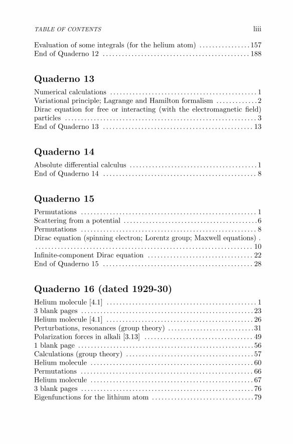
TABLE OF CONTENTS liii

Evaluation of some integrals (for the helium atom) . . . . . . . . . . . . . . . . 157End of Quaderno 12 . . . . . . . . . . . . . . . . . . . . . . . . . . . . . . . . . . . . . . . . . . . . . . 188

Quaderno 13

Numerical calculations . . . . . . . . . . . . . . . . . . . . . . . . . . . . . . . . . . . . . . . . . . . . . . 1Variational principle; Lagrange and Hamilton formalism . . . . . . . . . . . . . 2Dirac equation for free or interacting (with the electromagnetic field)particles . . . . . . . . . . . . . . . . . . . . . . . . . . . . . . . . . . . . . . . . . . . . . . . . . . . . . . . . . . . . 3End of Quaderno 13 . . . . . . . . . . . . . . . . . . . . . . . . . . . . . . . . . . . . . . . . . . . . . . . 13

Quaderno 14

Absolute differential calculus . . . . . . . . . . . . . . . . . . . . . . . . . . . . . . . . . . . . . . . . 1End of Quaderno 14 . . . . . . . . . . . . . . . . . . . . . . . . . . . . . . . . . . . . . . . . . . . . . . . . 8

Quaderno 15

Permutations . . . . . . . . . . . . . . . . . . . . . . . . . . . . . . . . . . . . . . . . . . . . . . . . . . . . . . . 1Scattering from a potential . . . . . . . . . . . . . . . . . . . . . . . . . . . . . . . . . . . . . . . . . .6Permutations . . . . . . . . . . . . . . . . . . . . . . . . . . . . . . . . . . . . . . . . . . . . . . . . . . . . . . . 8Dirac equation (spinning electron; Lorentz group; Maxwell equations) .. . . . . . . . . . . . . . . . . . . . . . . . . . . . . . . . . . . . . . . . . . . . . . . . . . . . . . . . . . . . . . . . . . . . 10Infinite-component Dirac equation . . . . . . . . . . . . . . . . . . . . . . . . . . . . . . . . . 22End of Quaderno 15 . . . . . . . . . . . . . . . . . . . . . . . . . . . . . . . . . . . . . . . . . . . . . . . 28

Quaderno 16 (dated 1929-30)

Helium molecule [4.1] . . . . . . . . . . . . . . . . . . . . . . . . . . . . . . . . . . . . . . . . . . . . . . . 13 blank pages . . . . . . . . . . . . . . . . . . . . . . . . . . . . . . . . . . . . . . . . . . . . . . . . . . . . . . 23Helium molecule [4.1] . . . . . . . . . . . . . . . . . . . . . . . . . . . . . . . . . . . . . . . . . . . . . . 26Perturbations, resonances (group theory) . . . . . . . . . . . . . . . . . . . . . . . . . . .31Polarization forces in alkali [3.13] . . . . . . . . . . . . . . . . . . . . . . . . . . . . . . . . . . 491 blank page . . . . . . . . . . . . . . . . . . . . . . . . . . . . . . . . . . . . . . . . . . . . . . . . . . . . . . . 56Calculations (group theory) . . . . . . . . . . . . . . . . . . . . . . . . . . . . . . . . . . . . . . . . 57Helium molecule . . . . . . . . . . . . . . . . . . . . . . . . . . . . . . . . . . . . . . . . . . . . . . . . . . . 60Permutations . . . . . . . . . . . . . . . . . . . . . . . . . . . . . . . . . . . . . . . . . . . . . . . . . . . . . . 66Helium molecule . . . . . . . . . . . . . . . . . . . . . . . . . . . . . . . . . . . . . . . . . . . . . . . . . . . 673 blank pages . . . . . . . . . . . . . . . . . . . . . . . . . . . . . . . . . . . . . . . . . . . . . . . . . . . . . . 76Eigenfunctions for the lithium atom . . . . . . . . . . . . . . . . . . . . . . . . . . . . . . . . 79

liv E. MAJORANA: RESEARCH NOTES ON THEORETICAL PHYSICS

Symmetric group . . . . . . . . . . . . . . . . . . . . . . . . . . . . . . . . . . . . . . . . . . . . . . . . . . 80Thomson formula for β particles in a medium [7.4] . . . . . . . . . . . . . . . . . 83Calculations (group theory; atomic eigenfunctions) . . . . . . . . . . . . . . . . . 84Ground state of the lithium atom (electrostatic potential) [3.8.1] . . . 98Self-consistent field in two-electron atoms [3.4] . . . . . . . . . . . . . . . . . . . . 100Numerical calculations . . . . . . . . . . . . . . . . . . . . . . . . . . . . . . . . . . . . . . . . . . . . 103Ground state of the lithium atom [3.8.2] . . . . . . . . . . . . . . . . . . . . . . . . . . 112Numerical calculations and tables . . . . . . . . . . . . . . . . . . . . . . . . . . . . . . . . . 114Helium atom; two-electron atoms . . . . . . . . . . . . . . . . . . . . . . . . . . . . . . . . . 134Asymptotic expansion . . . . . . . . . . . . . . . . . . . . . . . . . . . . . . . . . . . . . . . . . . . . 141Ground state of three-electron atoms [3.7] . . . . . . . . . . . . . . . . . . . . . . . . .1572s terms for two-electron atoms [3.5] . . . . . . . . . . . . . . . . . . . . . . . . . . . . . . 157Asymptotic behavior for the s terms in alkali [3.9] . . . . . . . . . . . . . . . . 158Calculations (group theory) . . . . . . . . . . . . . . . . . . . . . . . . . . . . . . . . . . . . . . . 174Numerical calculations . . . . . . . . . . . . . . . . . . . . . . . . . . . . . . . . . . . . . . . . . . . . 1754 blank pages . . . . . . . . . . . . . . . . . . . . . . . . . . . . . . . . . . . . . . . . . . . . . . . . . . . . . 185Eigenvalue equation . . . . . . . . . . . . . . . . . . . . . . . . . . . . . . . . . . . . . . . . . . . . . . 189End of Quaderno 16 . . . . . . . . . . . . . . . . . . . . . . . . . . . . . . . . . . . . . . . . . . . . . . 190

Quaderno 17 (dated 20 June 1932)

Proton-neutron scattering . . . . . . . . . . . . . . . . . . . . . . . . . . . . . . . . . . . . . . . . . . . 1Radioactivity [7.2] . . . . . . . . . . . . . . . . . . . . . . . . . . . . . . . . . . . . . . . . . . . . . . . . . . 5Nuclear potential (mean nucleon potential) [7.3.1] . . . . . . . . . . . . . . . . . . . 6Nuclear potential (interaction potential between nucleons) [7.3.2] . . . . 9Nuclear potential (nucleon density) [7.3.3] . . . . . . . . . . . . . . . . . . . . . . . . . .12Nuclear potential (nucleon interaction) [7.3.4] . . . . . . . . . . . . . . . . . . . . . . 14Nuclear potential (nucleon interaction) [7.3.5] . . . . . . . . . . . . . . . . . . . . . . 20Nuclear potential (simple nuclei) [7.3.6] . . . . . . . . . . . . . . . . . . . . . . . . . . . . 31Nuclear potential (simple nuclei) [7.3.7] . . . . . . . . . . . . . . . . . . . . . . . . . . . . 33Magnetic moment and diamagnetic susceptibility for a one-electron atom(relativistic calculation) [3.17] . . . . . . . . . . . . . . . . . . . . . . . . . . . . . . . . . . . . . . 36General transformations for matrices . . . . . . . . . . . . . . . . . . . . . . . . . . . . . . . 39Symmetrical theory of the electron and positron . . . . . . . . . . . . . . . . . . . 40General transformations for matrices . . . . . . . . . . . . . . . . . . . . . . . . . . . . . . . 43Dirac equation (real components); �A + λA = p . . . . . . . . . . . . . . . . . . . 45Maxwell equations in the Dirac-like form; spinor transformations (con-tinuation from p.159-160) . . . . . . . . . . . . . . . . . . . . . . . . . . . . . . . . . . . . . . . . . . 69Numerical calculations . . . . . . . . . . . . . . . . . . . . . . . . . . . . . . . . . . . . . . . . . . . . . 72Symmetrical theory of the electron and positron (continuation from p.40-42) . . . . . . . . . . . . . . . . . . . . . . . . . . . . . . . . . . . . . . . . . . . . . . . . . . . . . . . . . . . . . . . . 74

TABLE OF CONTENTS lv

Calculations . . . . . . . . . . . . . . . . . . . . . . . . . . . . . . . . . . . . . . . . . . . . . . . . . . . . . . . 82Maxwell equations in the Dirac-like form; spinor transformations . . . 831 blank page . . . . . . . . . . . . . . . . . . . . . . . . . . . . . . . . . . . . . . . . . . . . . . . . . . . . . . . 88? . . . . . . . . . . . . . . . . . . . . . . . . . . . . . . . . . . . . . . . . . . . . . . . . . . . . . . . . . . . . . . . . . . 89Dirac equation . . . . . . . . . . . . . . . . . . . . . . . . . . . . . . . . . . . . . . . . . . . . . . . . . . . . . 90Calculations (perturbation theory) . . . . . . . . . . . . . . . . . . . . . . . . . . . . . . . . . 923 blank pages . . . . . . . . . . . . . . . . . . . . . . . . . . . . . . . . . . . . . . . . . . . . . . . . . . . . . . 94Degenerate gas of spinless electrons [5.1] . . . . . . . . . . . . . . . . . . . . . . . . . . . 97Calculations (spherical harmonics; recursive relations) . . . . . . . . . . . . . . 98Phase space; classical and quantum “product” . . . . . . . . . . . . . . . . . . . . 1042 blank pages . . . . . . . . . . . . . . . . . . . . . . . . . . . . . . . . . . . . . . . . . . . . . . . . . . . . . 127Wave equation for the neutron [7.1] . . . . . . . . . . . . . . . . . . . . . . . . . . . . . . . 129Quantized radiation field [2.9] . . . . . . . . . . . . . . . . . . . . . . . . . . . . . . . . . . . . .129Free electron scattering [2.12] . . . . . . . . . . . . . . . . . . . . . . . . . . . . . . . . . . . . . 133Wave equation of light quanta [2.10] . . . . . . . . . . . . . . . . . . . . . . . . . . . . . . 142Bound electron scattering [2.13] . . . . . . . . . . . . . . . . . . . . . . . . . . . . . . . . . . .142Wave equation of light quanta (continuation from p.142) [2.11] . . . . 151Wavefunctions of a two-electron atom [3.2] . . . . . . . . . . . . . . . . . . . . . . . . 152Maxwell equations in the Dirac-like form; spinor transformations . . 156Atomic eigenfunctions (lithium) [3.11] . . . . . . . . . . . . . . . . . . . . . . . . . . . . 161Classical theory of multipole radiation . . . . . . . . . . . . . . . . . . . . . . . . . . . . 166Calculations (quantum mechanics) . . . . . . . . . . . . . . . . . . . . . . . . . . . . . . . . 167Atomic eigenfunctions (hydrogen) . . . . . . . . . . . . . . . . . . . . . . . . . . . . . . . . .171Calculations (quantum mechanics) . . . . . . . . . . . . . . . . . . . . . . . . . . . . . . . . 179Formulae (relativistic quantum mechanics) . . . . . . . . . . . . . . . . . . . . . . . . 183End of Quaderno 17 . . . . . . . . . . . . . . . . . . . . . . . . . . . . . . . . . . . . . . . . . . . . . . 190

Quaderno 18

Maxwell electrodynamics (variational principle) . . . . . . . . . . . . . . . . . . . . . 1Bessel functions; generalized Green functions; Hamilton equations . . . 8Scattering from a potential (Green functions) . . . . . . . . . . . . . . . . . . . . . . 18Scattering from a potential (α particles); Ritz method . . . . . . . . . . . . . .27Calculations (quantum field theory) . . . . . . . . . . . . . . . . . . . . . . . . . . . . . . . . 54Cubic symmetry . . . . . . . . . . . . . . . . . . . . . . . . . . . . . . . . . . . . . . . . . . . . . . . . . . . 55Thermodynamics; van der Waals equation . . . . . . . . . . . . . . . . . . . . . . . . . 59Calculations (quantum mechanics; perturbation theory) . . . . . . . . . . . . 66“Double” (second) quantization . . . . . . . . . . . . . . . . . . . . . . . . . . . . . . . . . . . . 69Calculations (permutations; Young tableaux) . . . . . . . . . . . . . . . . . . . . . . .74Atomic calculations (helium?); Dirac matrices; van der Waals curves 89Numerical calculations (helium? hydrogen?) . . . . . . . . . . . . . . . . . . . . . . 106

lvi E. MAJORANA: RESEARCH NOTES ON THEORETICAL PHYSICS

Differential equation . . . . . . . . . . . . . . . . . . . . . . . . . . . . . . . . . . . . . . . . . . . . . . 156Pauli paramagnetism [5.2] . . . . . . . . . . . . . . . . . . . . . . . . . . . . . . . . . . . . . . . . 157Helium (anomalous terms) . . . . . . . . . . . . . . . . . . . . . . . . . . . . . . . . . . . . . . . . 158End of Quaderno 18 . . . . . . . . . . . . . . . . . . . . . . . . . . . . . . . . . . . . . . . . . . . . . . 160

PART I

1

DIRAC THEORY

1.1. VIBRATING STRING

Starting from the problem of the vibrating string (which is studied in theframework of the canonical formalism), Majorana obtained a (classical)Dirac-like equation for a two-component field u = (u1, u2), where Paulimatrices σ appear.

−12

δ

∫ [(∂q

∂t

)2

−(

∂q

∂x

)2]

dτ = 0,

q =∂2q

∂x2, p =

∂q

∂t,

H =12

∫ [

p2 +(

∂q

∂x

)2]

dx,

(q1, p1) (q2, p2) (q3, p3) . . . ,

H =12

∑

λ

(λ2q2λ + p2

λ).

� =1c2

∂2

∂t− ∇2 =

(1c

∂

∂t+ σx

∂

∂x+ σy

∂

∂y+ σr

∂

∂z

)

×(

1c

∂

∂t− σx

∂

∂x− σy

∂

∂y− σz

∂

∂z

),

(1c

∂

∂t− σx

∂

∂xσy

∂

∂yσz

∂

∂z

)u = 0,

u = (u1, u2),

∂u

∂t= c

(σx

∂

∂x+ σy

∂

∂y+ σz

∂

∂z

)u,

3

4 E. MAJORANA: RESEARCH NOTES ON THEORETICAL PHYSICS

σx =∣∣∣∣

0 11 0

∣∣∣∣ , σy =

∣∣∣∣

0 −ii 0

∣∣∣∣ , σz =

∣∣∣∣

1 00 −1

∣∣∣∣ ,

1c

∂u1

∂t=

(∂

∂x− i

∂

∂y

)u2 +

∂

∂zu1,

1c

∂u2

∂t=

(∂

∂x+ i

∂

∂y

)u1 −

∂

∂zu2,

(1c

∂

∂t− ∂

∂z

)u1 =

(∂

∂x− i

∂

∂y

)u2,

(1c

∂

∂t+

∂

∂z

)u2 =

(∂

∂x+ i

∂

∂y

)u1.

x0 = ict,

x1 = x,

x2 = y,

x3 = z,

i

(∂

∂x0+ i

∂

∂x3

)u1 =

(∂

∂x1− ∂

∂x2

)u2,

i

(∂

∂x0− i

∂

∂x3

)u2 =

(∂

∂x1+

∂

∂x2

)u1.

1.2. A SEMICLASSICAL THEORY FOR THEELECTRON

1.2.1 Relativistic DynamicsIn the following, the relativistic equations of motion for an electron ina force field F are considered in a non-usual way, by separating theradial F r and the transverse component F t (with respect to the particlevelocity βc) of the force. Expressions for the time derivative of the chargedensity ρ and current density i, which satisfy the continuity equation,are obtained.

DIRAC THEORY 5

charge + e

mass m

ρ, ix = ρβx, iy = ρβy, iz = ρβz;

βx = vx/c, βy = vy/c, βz = vz/c;

β =√

β2x + β2

y + β2z = v/c.

ddt

mvx√1 − β2

= eFx,

ddt

mvy√1 − β2

= eFy,

ddt

mvz√1 − β2

= eFz.

k =e

mc.

ddt

β√

1 − β2=

1kF ,

ddt

β√

1 − β2=

β√

1 − β2+

(β · β)β(1 − β2)3/2

=1

√1 − β2

(

β +β · β

1 − β2β

)

,

1√

1 − β2β +

1(1 − β2)3/2

(β · β)β =1kF .

1kF · β =

1(1 − β2)3/2

(β · β),

1kF × β =

1√

1 − β2β × β;

βr = (1 − β2)3/2 1kF r,

βt =√

1 − β21kF t;

6 E. MAJORANA: RESEARCH NOTES ON THEORETICAL PHYSICS

β = βr + βt,

F = F r + F t.

F r =(

(Fxβx + Fyβy + Fzβz)βx

β2, (Fxβx + Fyβy + Fzβz)

βy

β2,

(Fxβx + Fyβy + Fzβz)βz

β2

),

F t =(

Fx − (Fxβx + Fyβy + Fzβz)βx

β2, Fy − (Fxβx + Fyβy + Fzβz)

βy

β2,

Fz − (Fxβx + Fyβy + Fzβz)βr

β2

).

βx =

√1 − β2

k[Fx − (Fxβx + Fyβy + Fzβz)βz] =

ddt

βx,

βy =

√1 − β2

k[Fx − (Fxβx + Fyβy + Fzβz)βz] =

ddt

βy,

βr =

√1 − β2

k[Fx − (Fxβy + Fyβy + Fzβz)βz] =

ddt

βz.

∂ρ

∂t+ c

(∂ix∂x

+∂iy∂y

+∂iz∂z

)= 0;

dρ

dt=

∂ρ

∂t+ c

(βx

∂ρ

∂x+ βy

∂ρ

∂y+ βz

∂ρ

∂z

);

dρ

dt= c

(βx

∂ρ

∂x+ βy

∂ρ

∂y+ βz

∂ρ

∂z− ∂ix

∂x− ∂iy

∂y− ∂iz

∂z

);

∂ix∂t

=dixdt

− c

(βx

∂ix∂x

+ βy∂iy∂y

+ βz∂iz∂z

);

dixdt

=ddt

(ρβx) = βxdρ

dt+ ρ

dβx

dt

= βx · c(

βx∂ρ

∂x+ βy

∂ρ

∂y+ βz

∂ρ

∂z− ∂ix

∂x− ∂iy

∂y− ∂iz

∂z

)

+ρ

√1 − β2

k[Fx − (Fxβx + Fyβy + Fzβz)βx] .

DIRAC THEORY 7

1.2.2 Field EquationsThe author began now to study the field equations for an electron in anelectromagnetic potential (ϕ,C) by following two different approaches.In the first part, he “tries” with a semiclassical Hamilton-Jacobi equationcorresponding to the relativistic expression for the energy-momentum re-lation, by imposing the constraint of a positive value for the energy.From appropriate correspondence relations, he then deduced a Klein-Gordon equation for the field ψ and, on introducing the Pauli matrices,the Dirac equations for the electron 4-component wavefunction. Some(mathematical) consequences of the formalism adopted (mainly relatedto the charge-current density) were also analyzed.In the second part, Majorana focused his attention on the standard for-malism for the Dirac equation, again discussing in detail the expressionsfor the Dirac charge-current density (ρ, i) and some peculiar constraintson Lorentz-invariant field quantities. He introduced and studied the con-sequences of several ansatz leading to Dirac-like equations for the elec-tron.

−(−1

c

∂S

∂t+

e

cϕ

)2

+∑

x

(∂S

∂x+

e

cCx

)2

+ m2c2 = 0;

−1c

∂S

∂t+

e

cϕ > 0 .

ψ = A e2πiS/h, A = |ψ|.

∂ψ

∂x=

(∂A

∂x+ A

2πi

h

∂S

∂x

)e2πiS/h =

(1A

∂A

∂x+

2πi

h

∂S

∂x

)ψ

∂2ϕ

∂x2=

(∂2A

∂x2+ 2

∂A

∂x

2πi

h

∂S

∂x+ A

2πi

h

∂S

∂x2− A

4π2

h2

∂S

∂x2

)e2πiS/h

=(

1A

∂2A

∂x2+

2A

2π

h

∂S

∂x+

2πi

h

∂2S

∂x2− 4π2

h2

∂S

∂x2

)ψ

Versuchsweise: 1

1@ This German word means “tentatively”, and refers to the successive assumptions. Note,however, that in the original paper the cited word is written as “versucherweiser”.

8 E. MAJORANA: RESEARCH NOTES ON THEORETICAL PHYSICS

⎧⎪⎪⎪⎪⎨

⎪⎪⎪⎪⎩

∂S

∂x=

h

2πi

1ψ

∂ψ

∂x;

∂S

∂t=

h

2πi

1ψ

∂ψ

∂t;

∂S

∂x= − h

2πi

1ψ

∂ψ

∂x;

∂S

∂t= − h

2πi

1ψ

∂ψ

∂t.

−[(

−1c

h

2πi

∂

∂t+

e

cϕ

)]2

+∑

x

[(h

2πi

∂

∂x+

e

cCx

)ψ

]2

+m2c2ψ2 = 0. (B)

Approximate condition:

ψ

(−1

c

h

2πi

∂

∂t+

e

cϕ

)ψ + ψ

(1c

h

2πi

∂

∂t+ eϕ

)ψ > 0.

In exact form:

−(−1

c

∂S

∂t+

e

cϕ

)2

+∑

x

(∂S

∂x+

e

cCx

)2

+ m2c2 = 0, (A)

|ψ| = 1; (C)

ψ = e2πiS/h,

∂ψ

∂x=

2πi

h

∂S

∂xψ.

(A) ≡ (B) + (C).

ψ0 = sin2π

hS, ψ1 = cos

2π

hS;

∂ψ0

∂x=

2π

h

∂S

∂xcos

2π

hS,

∂ψ1

∂x= −2π

h

∂S

∂xsin

2π

hS;

h

2π

∂ψ0

∂x=

∂S

∂xψ1,

h

2π

∂ψ1

∂x= −∂S

∂xψ0,

DIRAC THEORY 9

∂S

∂x=

1ψ1

h

2π

∂ψ0

∂x= − 1

ψ0

h

2π

∂ψ1

∂x.

——————–

δ

∫ {(1c

h

2π

∂ϕ0

∂t− e

cϕψ1

)(1c

h

2π

∂ψ1

∂t+

e

cϕψ0

)

+∑

x

(h

2π

∂ψ0

∂x+

e

cCxψ1

)(h

2π

∂ψ1

∂x− e

cCxψ0

)+ m2c2ψ0ψ1

}

dτ = 0

(dτ = dV dt). 2

h

2π

∂

∂t

(1c

h

2π

∂ψ0

∂t− e

cϕψ1

)+

e

cϕ

(1c

h

2π

∂ϕ1

∂t+

e

cϕψ0

)

−∑

x

[h

2π

∂

∂x

(h

2π

∂ψ0

∂x+

e

cCxϕ1

)− e

cCx

(22π

∂ψ1

∂x− e

cCxψ0

)]

+m2c2ψ0 = 0.

[−1

c

h

2πi

∂

∂t+

e

cϕ + ρ3 σ ·

(h

2πi∇ +

e

cC

)+ ρ1mc

]ψ = 0,

σx =∣∣∣∣

0 11 0

∣∣∣∣ , σy =

∣∣∣∣

0 −ii 0

∣∣∣∣ , σz =

∣∣∣∣

1 00 −1

∣∣∣∣ ;

A = (ψ1, ψ2), B = (ψ3, ψ4).

[−1

c

h

2πi

∂

∂t+

e

cϕ + σ ·

(h

2πi∇ +

e

cC

)]A + mcB = 0,

[−1

c

h

2πi

∂

∂t+

e

cϕ − σ ·

(h

2πi∇ +

e

cC

)]B + mcA = 0.

ρ = AA + BB = ψ1ψ1 + ψ2ψ2 + ψ3ψ3 + ψ4ψ4,

ix = AσxA + BσxB = −ψ1ψ2 − ψ2ψ1 + ψ3ψ4 + ψ4ψ3,

iy = AσyA + BσyB = i(ψ1ψ2 − ψ2ψ1 − ψ3ψ4 + ψ4ψ3),

iz = AσrA + BσrB = −ψ1ψ1 + ψ2ψ2 + ψ3ψ3 − ψ4ψ4.

2@ Note that, more appropriately, it should be written d4τ = d3V dt, since dτ denotes the4-dimensional volume element, while drmV is the 3-dimensional space volume element.

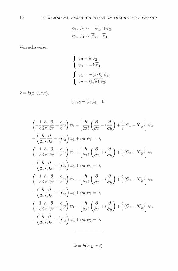
10 E. MAJORANA: RESEARCH NOTES ON THEORETICAL PHYSICS

ψ1, ψ2 ∼ −ψ4, +ψ3,

ψ3, ψ4 ∼ ψ2, −ψ1.

Versuchsweise:{

ψ3 = k ψ2,

ψ4 = −k ψ1;{

ψ1 = −(1/k) ψ4,

ψ2 = (1/k) ψ3;

k = k(x, y, r, t),

ψ1ψ3 + ψ2ψ4 = 0.

(−1

c

h

2πi

∂

∂t+

e

cϕ

)ψ1 +

[h

2πi

(∂

∂x− i

∂

∂y

)+

e

c(Cx − iCy)

]ψ2

+(

h

2πi

∂

∂z+

e

cCz

)ψ1 + mcψ3 = 0,

(−1

c

h

2πi

∂

∂t+

e

cϕ

)ψ2 +

[h

2πi

(∂

∂x+ i

∂

∂y

)+

e

c(Cx + iCy)

]ψ1

−(

h

2πi

∂

∂z+

e

cCz

)ψ2 + mcψ4 = 0,

(−1

c

h

2πi

∂

∂t+

e

cϕ

)ψ3 −

[h

2πi

(∂

∂x− i

∂

∂y

)+

e

c(Cx − iCy)

]ψ4

−(

h

2πi

∂

∂z+

e

cCz

)ψ3 + mcψ1 = 0,

(−1

c

h

2πi

∂

∂t+

e

cϕ

)ψ4 −

[h

2πi

(∂

∂x+ i

∂

∂y

)+

e

c(Cx + iCy)

]ψ3

+(

h

2πi

∂

∂z+

e

cCz

)ψ4 + mcψ2 = 0.

——————–

k = k(x, y, r, t)

DIRAC THEORY 11(−1

c

h

2πi

∂

∂t+

e

cϕ

)ψ1 +

[h

2πi

(∂

∂x− i

∂

∂y

)+

e

c(Cx − iCy)

]ψ2

+(

h

2πi

∂

∂z+

e

cCz

)ψ1 + kmcψ2 = 0,

(−1

c

h

2πi

∂

∂t+

e

cϕ

)ψ2 +

[h

2πi

(∂

∂x+ i

∂

∂y

)+

e

c(Cx + iCy)

]ψ1

−(

h

2πi

∂

∂z+

e

cCz

)ψ2 − kmcψ1 = 0,

(−1

c

h

2πi

∂

∂t+

e

cϕ

)(kψ2) −

[h

2πi

(∂

∂x− i

∂

∂y

)+

e

c(Cx − iCy)

](−kψ1)

−(

h

2πi

∂

∂z+

e

cCz

)(kψ2) + mcψ1 = 0,

(−1

c

h

2πi

∂

∂t+

e

cϕ

)(−kψ1) −

[h

2πi

(∂

∂x+ i

∂

∂y

)+

e

c(Cx + iCy)

](kψ2)

+(

h

2πi

∂

∂z+

e

cCz

)(−kψ1) + mcψ2 = 0.

——————–

without field3 : k = ±1; ψ3 = ψ2; ψ4 = −ψ1; ϕ,C = 0

−1c

h

2πi

∂

∂tψ1 +

h

2πi

(∂

∂x− i

∂

∂y

)ψ2 +

h

2πi

∂

∂rψ1 + mcψ2 = 0,

−1c

h

2πi

∂

∂tψ2 +

h

2πi

(∂

∂x+ i

∂

∂y

)ψ1 −

h

2πi

∂

∂rψ2 − mcψ1 = 0,

−1c

h

2πi

∂

∂tψ2 +

h

2πi

(∂

∂x− i

∂

∂y

)ψ1 −

h

2πi

∂

∂rψ2 + mcψ1 = 0,

+1c

h

2πi

∂

∂tψ1 −

h

2πi

(∂

∂x+ i

∂

∂y

)ψ2 −

h

2πi

∂

∂rψ1 + mcψ2 = 0.

For real u1, u2, u3, u4:

3@ This interesting side note is present in the original manuscript: we can use ±m in placeof k = ±1: k = 1 corresponds to m and k = −1 corresponds to −m.

12 E. MAJORANA: RESEARCH NOTES ON THEORETICAL PHYSICS

k = 1 : ψ1 =u1 + iu2√

2, ψ2 =

u3 + iu4√2

,

ψ3 =u3 − iu4√

2, ψ4 =

−u1 + iu2√2

;

k = −1 : ψ1 =u1 + iu2√

2, ψ2 =

u3 + iu4√2

,

ψ3 =−u3 + iu4√

2, ψ4 =

u1 − iu2√2

.

ρ = u21 + u2

2 + u23 + u2

4,

ix = − (2u1u3 + 2u2u4) ,

iy = − (2u1u4 − 2u2u3) ,

iz = −(u2

1 + u22 − u2

3 − u24

).

1c

h

2π

∂

∂tu1 −

h

2π

∂

∂xu3 −

h

2π

∂

∂yu4 −

h

2π

∂

∂zu1 − mcu4 = 0,

1c

h

2π

∂

∂tu2 −

h

2π

∂

∂xu4 +

h

2π

∂

∂yu3 −

h

2π

∂

∂zu2 − mcu3 = 0,

1c

h

2π

∂

∂tu3 −

h

2π

∂

∂xu1 +

h

2π

∂

∂yu2 +

h

2π

∂

∂zu3 + mcu2 = 0,

1c

h

2π

∂

∂tu4 −

h

2π

∂

∂xu2 −

h

2π

∂

∂yu1 +

h

2π

∂

∂zu4 + mcu1 = 0.

1c

h

2π

∂

∂tu =

[h

2π

(γ1

∂

∂x+ γ2

∂

∂y+ γ3

∂

∂r

)+ δ mc

]u.

γ1 =

∣∣∣∣∣∣∣∣

0 0 1 00 0 0 11 0 0 00 1 0 0

∣∣∣∣∣∣∣∣

, γ2 =

∣∣∣∣∣∣∣∣

0 0 0 10 0 −1 00 −1 0 01 0 0 0

∣∣∣∣∣∣∣∣

,

γ3 =

∣∣∣∣∣∣∣∣

1 0 0 00 1 0 10 0 −1 00 0 0 −1

∣∣∣∣∣∣∣∣

, δ =

∣∣∣∣∣∣∣∣

0 0 0 10 0 1 00 −1 0 0−1 0 0 0

∣∣∣∣∣∣∣∣

.

γ1 = ρ1, γ2 = −σyρ2, γ3 = ρ3, δ = −iσxρ2.

DIRAC THEORY 13

For u = u(r, t):

h

2π

(1c

∂

∂t− ∂

∂z

)u1 = mcu4,

h

2π

(1c

∂

∂t− ∂

∂z

)u2 = mcu3,

h

2π

(1c

∂

∂t+

∂

∂z

)u3 = −mcu2,

h

2π

(1c

∂

∂t+

∂

∂z

)u4 = −mcu1;

u1 = λ1R e2πih

(−at+bz),

u2 = λ2R e2πih

(−at+bz),

u3 = λ3R e2πih

(−at+bz),

u1 = λ4R e2πih

(−at+bz).

−i(a

c+ b

)λ1 = mcλ4,

−i(a

c+ b

)λ2 = mcλ3,

−i(a

c− b

)λ3 = −mcλ2,

−i(a

c− b

)λ4 = −mcλ1;

a2

c2= m2c2 + b2,

λ4

λ1= − i

mc

(a

c+ b

)=

λ3

λ2.

——————–

ρ = u†L0u, ix = u†L1u, iy = u†L2u, iz = u†L3u;

L0 =

∣∣∣∣∣∣∣∣

1 0 0 00 1 0 00 0 1 00 0 0 1

∣∣∣∣∣∣∣∣

, L1 = −

∣∣∣∣∣∣∣∣

0 0 1 00 0 0 11 0 0 01 0 0 0

∣∣∣∣∣∣∣∣

= −γ1,

14 E. MAJORANA: RESEARCH NOTES ON THEORETICAL PHYSICS

L2 = −

∣∣∣∣∣∣∣∣

0 0 0 10 0 −1 00 −1 0 01 0 0 0

∣∣∣∣∣∣∣∣

= −γ2, L3 = −

∣∣∣∣∣∣∣∣

1 0 0 00 1 0 00 0 −1 00 0 0 −1

∣∣∣∣∣∣∣∣

= −γ3.

ρ2 = (u21 + u2

2 + u23 + u2

4)2

= u41 + u4

2 + u43 + u4

4 + 2u21u

22 + 2u2

1u23 + 2u2

1u24 + 2u2

2u23

+2u22u

24 + 2u2

3u24,

i2x = 4(u1u3 + u2u4)2 = 4u21u

23 + 4u2

2u24 + 8u1u2u3u4,

i2y = 4(u1u4 − u2u3)2 = 4u21u

24 + 4u2

2u23 − 8u1u2u3u4,

i2z = (u21 + u2

2 − u23 − u2

4)2,

= u41 + u4

2 + u43 + u2

4 + 2u21u

22 − 2u2

1u23 − 2u2

1u24 − 2u2

2u23

−2u22u

24 + 2u2

3u24;

ρ2 − i2x − i2y − i2z = 0.

——————–

(ψ1ψ1 + ψ2ψ2 + ψ3ψ3 + ψ4ψ4)2 = ψ21ψ

21 + ψ

22ψ

22 + ψ

23ψ

23 + ψ

24ψ

24

+ 2ψ1ψ2ψ1ψ2 + 2ψ1ψ3ψ1ψ3 + 2ψ1ψ4ψ1ψ4 + 2ψ2ψ3ψ2ψ3

+ ψ2ψ4ψ2ψ4 + 2ψ3ψ4ψ3ψ4,

(−ψ1ψ2 − ψ2ψ1 + ψ3ψ4 + ψ4ψ3)2 = ψ21ψ

22 + ψ

22ψ

21 + ψ

23ψ

24 + ψ

24ψ

23

+ 2ψ1ψ2ψ1ψ2 − 2ψ1ψ3ψ2ψ4 − 2ψ1ψ4ψ2ψ3 − 2ψ2ψ3ψ1ψ4

− 2ψ2ψ4ψ1ψ3 + 2ψ3ψ4ψ3ψ4,

−(ψ1ψ2 − ψ2ψ1 − ψ3ψ4 + ψ4ψ3)2 = −ψ21ψ

22 − ψ

22ψ

21 − ψ

23ψ

24 − ψ

24ψ

23

+ 2ψ1ψ2ψ1ψ2 + 2ψ1ψ3ψ2ψ4 − 2ψ1ψ4ψ2ψ3 − 2ψ2ψ3ψ1ψ4

+ 2ψ2ψ4ψ1ψ3 + 2ψ3ψ4ψ3ψ4,

(−ψ1ψ1 + ψ2ψ2 + ψ3ψ3 − ψ4ψ4)2 = ψ21ψ

21 + ψ

22ψ

22 + ψ

23ψ

23 + ψ

24ψ

24

− 2ψ1ψ2ψ1ψ2 − 2ψ21ψ

23ψ1ψ3 + 2ψ1ψ4ψ1ψ4 + 2ψ2ψ3ψ2ψ3

− 2ψ2ψ4ψ2ψ4 − 2ψ3ψ4ψ3ψ4.

ρ2 − i2z = 4ψ1ψ2ψ1ψ2 + 4ψ1ψ3ψ1ψ3 + 4ψ2ψ4ψ2ψ4 + 4ψ3ψ4ψ3ψ4,

i2x + i2y = 4ψ1ψ2ψ1ψ2 − 4ψ1ψ4ψ2ψ3 − 4ψ2ψ3ψ1ψ4 + 4ψ3ψ4ψ3ψ4.

DIRAC THEORY 15

ρ2 − i2x − i2y − i2r = 4ψ1ψ3ψ1ψ3 + 4ψ2ψ4ψ2ψ4 + 4ψ1ψ4ψ2ψ3

+ 4ψ2ψ3ψ1ψ4

= 4(ψ1ψ3 + ψ2ψ4)(ψ1ψ3 + ψ2ψ4) = QQ;

Q = 2(ψ1ψ3 + ψ2ψ4), Q = (ψ1ψ3 + ψ2ψ4).

——————–[(

W

c+

e

cϕ

)+ ρ3

∑

x

σx

(px +

e

cCx

)+ ρ1mc

]

ψ = 0.

δ

∫ψ

[W

c+

e

cϕ + ρ3

∑

x

σx

(px +

e

cCx

)+ ρ1mc

]

ψ dτ = 0;

dτ = dV dt.ψ1ψ3 + ψ2ψ4 − ψ1ψ3 − ψ4ψ2 = 0.

δ

∫ {

ψ

[W

c+

e

cϕ + ρ3

∑

x

σx

(px +

e

cCx

)+ ρ1mc

]

ψ

+ λ i(ψ1ψ3 + ψ2ψ4 − ψ1ψ3 − ψ2ψ4)

}

dτ = 0.

∣∣∣∣∣∣∣∣

0 0 i 00 0 0 i−i 0 0 00 −i 0 0

∣∣∣∣∣∣∣∣

= −ρ2.

δ

∫ψ

[W

c+

e

cϕ + ρ3

∑

x

σx

(px +

e

cCx

)+ ρ1mc − λρ2

]

ψ dτ = 0.

⎧⎪⎪⎪⎨

⎪⎪⎪⎩

[W

c+

e

cϕ + ρ3

∑

x

σx

(px +

e

cCx

)+ ρ1mc

]

ϕ = λ ρ2ψ,

ψρ2ψ = 0.

ρ3σx = αx, ρ3σy = αy, ρ3σz = αz, ρ1 = α4, ρ2 = α5;

16 E. MAJORANA: RESEARCH NOTES ON THEORETICAL PHYSICS

αiαk + αkαi = 2δik;

α = (αx, αy, αz).

[W

c+

e

cϕ + α ·

(p +

e

cC

)+ α4mc

]ψ = α5λψ, ψα5ψ = 0.

−W

cψ =

[e

cϕ + α ·

(p +

e

cC

)+ α4mc − α5λ

]ψ,

−ψα5W

cψ =

e

cϕ ψα5ψ−

∑

x

ψαxα5

(px +

e

cCx

)ψ− ψα4α5 mcψ−λψψ.

A = (ψ1, ψ2), B(ψ3, ψ4).

[W

c+

e

cϕ + σ ·

(p +

e

cC

)]A + mcB = −λ iB,

BA − AB = 0.

[W

c+

e

cϕ − σ ·

(p +

e

cC

)]B + mcA = λ iB.

(−1

c

h

2πi

∂

∂t+

e

cϕ

)ψ1 +

[h

2πi

(∂

∂x− i

∂

∂y

)+

e

c(Cx − iCy)

]ψ2

+(

h

2πi

∂

∂z+

e

cCz

)ψ1 + mcψ3 = −λ iψ3,

(−1

c

h

2πi

∂

∂t+

e

cϕ

)ψ2 +

[h

2πi

(∂

∂x+ i

∂

∂y

)+

e

c(Cx + iCy)

]ψ1

−(

h

2πi

∂

∂z+

e

cCz

)ψ2 + mcψ4 = −λ iψ4,

(−1

c

h

2πi

∂

∂t+

e

cϕ

)ψ3 −

[h

2πi

(∂

∂x− i

∂

∂y

)+

e

c(Cx − iCy)

]ψ4

−(

h

2πi

∂

∂z+

e

cCz

)ψ3 + mcψ1 = λ iψ1,

(−1

c

h

2πi

∂

∂t+

e

cϕ

)ψ4 −

[h

2πi

(∂

∂x+ i

∂

∂y

)+

e

c(Cx − iCy)

]ψ3

+(

h

2πi

∂

∂z+

e

cCz

)ψ4 + mcψ2 = λ iψ2.

DIRAC THEORY 17

ψ1ψ3 + ψ2ψ4 − ψ3ψ1 − ψ4ψ2 = 0.

(1c

h

2πi

∂

∂t+

e

cϕ

)ψ1 −

[h

2πi

(∂

∂x+ i

∂

∂y

)− e

c(Cx + iCy)

]ψ2

−(

h

2πi

∂

∂z− e

cCz

)ψ1 + mcψ3 = λ iψ3,

(1c

h

2πi

∂

∂t+

e

cϕ

)ψ2 −

[h

2πi

(∂

∂x− i

∂

∂y

)− e

c(Cx − iCy)

]ψ1

+(

h

2πi

∂

∂z− e

cCz

)ψ2 + mcψ4 = λ iψ4,

(1c

h

2πi

∂

∂t+

e

cϕ

)ψ3 +

[h

2πi

(∂

∂x+ i

∂

∂y

)− e

c(Cx + iCy)

]ψ4

+(

h

2πi

∂

∂z− e

cCz

)ψ3 + mcψ1 = −λ iψ1,

(1c

h

2πi

∂

∂t+

e

cϕ

)ψ4 +

[h

2πi

(∂

∂x− i

∂

∂y

)− e

c(Cx − iCy)

]ψ3

−(

h

2πi

∂

∂z− e

cCz

)ψ4 + mcψ2 = −λ iψ2.

1c

h

2πi

∂

∂t(ψ1ψ3 + ψ2ψ4 − ψ3ψ1 − ψ4ψ2)

= ψ1

e

cϕψ3 − ψ1

[h

2πi

(∂

∂x− i

∂

∂y

)+

e

c(Cx − iCy)

]ψ4

−ψ1

(h

2πi

∂

∂z+

e

cCz

)ψ3 + mcψ1ψ1 − λ iψ1ψ1

+ψ2

e

cϕψ4 − ψ2

[h

2πi

(∂

∂x+ i

∂

∂y

)+

e

c(Cx + iCy)

]ψ3

+ψ2

(h

2πi

∂

∂z+

e

cCz

)ψ4 + mcψ2ψ2 − λ iψ2ψ2

−ψ3

e

cϕψ1 − ψ3

[h

2πi

(∂

∂x− i

∂

∂y

)+

e

c(Cx − iCy)

]ψ2

−ψ3

(h

2πi

∂

∂z+

e

cCz

)ψ1 − mcψ3ψ3 − λ iψ3ψ3

−ψ4

e

cϕψ2 − ψ4

[h

2πi

(∂

∂x+ i

∂

∂y

)+

e

c(Cx − iCy)

]ψ1

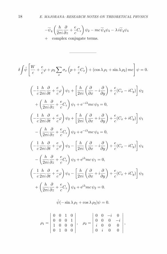
18 E. MAJORANA: RESEARCH NOTES ON THEORETICAL PHYSICS

−ψ4

(h

2πi

∂

∂z+

e

cCz

)ψ2 − mcψ4ψ4 − λ iψ4ψ4

+ complex conjugate terms.

——————–

δ

∫ψ

[W

c+

e

cϕ + ρ3

∑

x

σx

(p +

e

cCx

)+ (cos λ ρ1 + sin λ ρ2) mc

]

ψ = 0.

(−1

c

h

2πi

∂

∂t+

e

cϕ

)ψ1 +

[h

2πi

(∂

∂x− i

∂

∂y

)+

e

c(Cx − iCy)

]ψ2

+(

h

2πi

∂

∂z+

e

cCz

)ψ1 + e−iλmcψ3 = 0,

(−1

c

h

2πi

∂

∂t+

e

cϕ

)ψ2 +

[h

2πi

(∂

∂x+ i

∂

∂y

)+

e

c(Cx + iCy)

]ψ1

−(

h

2πi

∂

∂z+

e

cCz

)ψ2 + e−iλmcψ4 = 0,

(−1

c

h

2πi

∂

∂t+

e

cϕ

)ψ3 −

[h

2πi

(∂

∂x− i

∂

∂y

)+

e

c(Cx − iCy)

]ψ4

−(

h

2πi

∂

∂z+

e

cCz

)ψ3 + eiλmcψ1 = 0,

(−1

c

h

2πi

∂

∂t+

e

cϕ

)ψ4 −

[h

2πi

(∂

∂x+ i

∂

∂y

)+

e

c(Cx + iCy)

]ψ3

+(

h

2πi

∂

∂z+

e

cCz

)ψ4 + eiλmcψ2 = 0.

ψ(− sin λ ρ1 + cos λ ρ2)ψ = 0.

ρ1 =

∣∣∣∣∣∣∣∣

0 0 1 00 0 0 11 0 0 00 1 0 0

∣∣∣∣∣∣∣∣

, ρ2 =

∣∣∣∣∣∣∣∣

0 0 −i 00 0 0 −ii 0 0 00 i 0 0

∣∣∣∣∣∣∣∣

,

DIRAC THEORY 19

cos λ ρ1 + sin λ ρ2 =

∣∣∣∣∣∣∣∣

0 0 e−iλ 00 0 0 e−iλ

eiλ 0 0 00 eiλ 0 0

∣∣∣∣∣∣∣∣

,

− sin λ ρ1 + cos λ ρ2 =

∣∣∣∣∣∣∣∣

0 0 −ie−iλ 00 0 0 −ie−iλ

ieiλ 0 0 00 ieiλ 0 0

∣∣∣∣∣∣∣∣

.

ψ(− sin λ ρ1 + cos λ ρ2)ψ

= (1/i)(e−iλψ1ψ3 + e−iλψ2ψ4 − eiλψ3ψ1 − eiλψ4ψ2

)= 0.

e−iλ(ψ1ψ3 + ψ2ψ4) − eiλ(ψ3ψ1 + ψ4ψ2) = 0.

1c

h

2πi

∂

∂t

(e−iλψ1ψ3 + e−iλψ2ψ4 − eiλψ3ψ1 − eiλψ4ψ2

)

= −1c

h

2π(e−iλψ1ψ3 + e−iλψ2ψ4 + eiλψ3ψ2 + eiλψ4ψ2)

∂λ

∂t+ D + D,

D = e−iλ

{ψ1

e

cϕψ3 − ψ1

[h

2πi

(∂

∂x− i

∂

∂y

)+

e

c(Cx − iCy)

]ψ4

−ψ1

(h

2πi

∂

∂z+

e

cCz

)ψ3 + eiλmcψ1ψ1

}

+ e−iλ

{ψ2

e

cϕψ4 − ψ2

[h

2πi

(∂

∂x+ i

∂

∂y

)+

e

c(Cx + iCy)

]ψ3

+ψ2

(h

2πi

∂

∂z+

e

cCz

)ψ4 + eiλmcψ2ψ2

}

+ e+iλ

{ψ3

e

cϕψ1 + ψ3

[h

2πi

(∂

∂x− i

∂

∂y

)+

e

c(Cx − iCy)

]ψ2

+ψ3

(h

2πi

∂

∂z+

e

cCz

)ψ1 + e−iλmcψ3ψ3

}

+ e+iλ

{ψ4

e

cϕψ2 + ψ4

[h

2πi

(∂

∂x+ i

∂

∂y

)+

e

c(Cx + iCy)

]ψ1

−ψ4

(h

2πi

∂

∂z+

e

cCz

)ψ2 + e−iλmcψ4ψ4

}

20 E. MAJORANA: RESEARCH NOTES ON THEORETICAL PHYSICS

= −e

cCx

[e−iλ(+ψ1ψ4 + ψ2ψ3) + eiλ(ψ3ψ2 + ψ4ψ1)

]

+e

cCy

[i e−iλ(ψ1ψ4 − ψ2ψ3) − i eiλ(ψ4ψ1 − ψ3ψ2)

]

−e

cCz

[e−iλ(ψ1ψ3 − ψ2ψ4) + eiλ(ψ3ψ1 − ψ4ψ2)

]

+mc(ψ1ψ1 + ψ2ψ2 − ψ3ψ3 − ψ4ψ4

)

− h

2πi

[(ψ1

∂

∂xψ4 + ψ2

∂

∂xψ3

)e−iλ +

(ψ3

∂

∂xψ2 + ψ4

∂

∂xψ1

)eiλ

]

+h

2πi

[(ψ1

∂

∂yψ4 − ψ2

∂

∂xψ3

)e−iλ +

(ψ3

∂

∂xψ2 − ψ4

∂

∂xψ1

)eiλ

]

− h

2πi

[(ψ1

∂

∂zψ1 − ψ2

∂

∂zψ4

)e−iλ +

(ψ3

∂

∂zψ1 − ψ4

∂

∂zψ2

)eiλ

].

[4]

β =

∣∣∣∣∣∣∣∣

0 0 e−iλ 00 0 0 e−iλ

e−iλ 0 0 00 e−iλ 0 0

∣∣∣∣∣∣∣∣

,

γ =

∣∣∣∣∣∣∣∣

0 0 −ie−iλ 00 0 0 −ie−iλ

ieiλ 0 0 00 eiλ 0 0

∣∣∣∣∣∣∣∣

.

ψ =

∣∣∣∣∣∣∣∣

ψ1

ψ2

ψ3

ψ4

∣∣∣∣∣∣∣∣

,ψ† = |ψ1, ψ2, ψ3, ψ4),

ψ = |ψ1ψ2ψ3ψ4).

β = β(λ), γ = γ(λ);

β = cos λ ρ1 + sin λ ρ2, γ = − sin λ ρ1 + cos λ ρ2;

βγ = γβ = 0, β2 = γ2 = 1.

ψγψ = 0.

4@ Note that some things in the last three square brackets (the x, y, z-derivatives and theindices 1, 2, 3, 4 of the ψ components) should be slightly corrected. However, at variance withwhat is usually done by us, we choose to leave unchanged the expressions appearing in theoriginal manuscript.

DIRAC THEORY 21

0 = −1c

h

2πψβψ

∂λ

∂t− 2

e

cψβσ · Cψ − ψβσ · pψ + ψ†βσ · pψ.

——————–

ψβψ = e−iλ(ψ1ψ3 + ψ2ψ4) + eiλ(ψ3ψ1 + ψ4ψ2) = 2e−iλ(ψ1ψ3 + ψ2ψ4).

1c

h

2π

∂

∂t(e−iλψ1ψ3 + e−iλψ2ψ4 + eiλψ3ψ1 + eiλψ4ψ2)

=1c

h

2π

(−i e−iλψ1ψ3 − i e−iλψ2ψ4 + i eiλψ3ψ1 + i eiλψ4ψ1

) ∂λ

∂t+ L + L,

L = i e−iλ

{ψ2

e

cϕψ3 − ψ1

[h

2π

(∂

∂x− i

∂

∂y

)+

e

c(Cx − iCy)

]ψ4 − . . .

}

+ i e−iλ

{. . .

}

+ i e+iλ

{. . .

}

+ i e+iλ

{. . .

}

= ie

cϕ[e−iλ(ψ1ψ3 + ψ2ψ4) + eiλ(ψ3ψ1 + ψ4ψ2)

]

+ ie

cCx

[e−iλ(ψ1ψ4 + ψ2ψ3) − eiλ(ψ3ψ2 + ψ4ψ1)

]

+ ie

cCy

[. . .

]

± ie

cCz

[. . .

]

− h

2π

[(ψ1

∂

∂xψ4 + ψ2

∂

∂xψ3)e−iλ −

(ψ3

∂

∂xψ2 + ψ4

∂

∂xψ1

)eiλ

]

− h

2π

[. . .

]

− h

2π

[. . .

].

22 E. MAJORANA: RESEARCH NOTES ON THEORETICAL PHYSICS

1c

h

2π

∂

∂t(ψβψ) = 2

e

cψγ σ · C ψ + ψγ σ · pψ − ψxγ σ · pψ.

——————–

e−iλ(ψ1ψ3 + ψ2ψ4) − eiλ(ψ3ψ1 + ψ4ψ2) = 0.

eiλ =

√ψ1ψ3 + ψ2ψ4

ψ3ψ1 + ψ4ψ2

; e−iλ(ψ1ψ3 + ψ2ψ4) > 0;

|ψ1ψ3 + ψ2ψ| > 0,

provided that not all ψi be zero (ψ1 = ψ2 = ψ3 = ψ4 = 0) at the sametime.

1.3. QUANTIZATION OF THE DIRAC FIELD

The canonical quantization of a Dirac field ψ is here considered (start-ing from a Lagrangian density L), by introducing the field variables P, Pconjugate to ψ,ψ. After imposing the commutation rules, the Hamilto-nian H was deduced, and an expression for the energy W was obtainedin terms of the annihilation and creation operators a, b. The quantitiesni are number operators.

WA = V A − cσ · p B − mc2A,

WB = V B − cσ · pA − mc2B.

W0B0 =(

V +p2

2m+ mc2

)B0,

A0 = − σ · pB0

2mc.

W = − h

2πi

∂

∂tpx =

h

2πi

∂

∂x

L =1

2m

{(−W

c+

e

cϕ

)ψ

(W

c+

e

cϕ

)ψ

+∑

x

(−px +

e

cAx

)ψ

(px +

e

cAx

)ψ + m2c2 ψψ

}

.

DIRAC THEORY 23

ψ, P =(−W

c+

e

cϕ

)ψ;

ψ, P =(

W

c+

e

cϕ

)ψ.

ψ(q) ψ(q′) − ψ(q′) ψ(q) = 0, P (q) P (q′) − P (q′) P (q) = 0,

ψ(q) ψ(q′) − ψ(q′) ψ(q) = 0, P (q) P (q′) − P ′(q) P (q) = 0,

ψ(q) ψ(q′) − ψ(q′) ψ(q) = 0, P (q) P (q′) − P (q′) P (q) = 0.

ψ(q) P (q′) − P (q′) ψ(q) = δ(q − q′) 2mc,

ψ(q) P (q′) − P (q′) ψ(q) = 0,

ψ(q) P (q′) − P (q′) ψ(q) = 0,

ψ(q) P (q′) − P (q′) ψ(q′) = −δ(q − q′) 2mc.

H =1

2m

{(−W

c+

e

cϕ

)ψ

W

cψ +

(W

c+

e

cϕ

)ψ

W

cψ

}− L

=1

2m

{P (P − e

cϕψ

)+ P

(P − e

cϕψ

)− PP

+∑

x

(−px +

e

cAx

)ψ

(px +

e

cAx

)ψ + m2c2 ψψ

=1

2m

{PP − e

cϕ (Pψ + Pψ)

+∑

x

(−px +

e

cAx

)ψ

(px +

e

cAx

)ψ + m2c2 ψψ

}

.

a, a; b, b.

ab − ba = 2mc,

ab − ba = −2mc.

n =1

2√

mc

{1

4√

m2c2 + p2b + 4

√m2c2 + p2a

}

,

n′ =1

2√

mc

{1

4√

m2c2 + p2b − 4

√m2c2 + p2a

}

.

24 E. MAJORANA: RESEARCH NOTES ON THEORETICAL PHYSICS

1 + n1 + n2 =1

2mc

[1

√m2c2 + p2

bb +√

m2c2 + p2aa

]

,

n1 − n2 =1

2mc

[ab + ab

];

n1 =1

4mc

{1

4√

m2c2 + p2b + 4

√m2c2 + p2 a

}

×{

14√

m2c2 + p2b + 4

√m2c2 + p2 a

}

,

n2 =1

4mc

{1

4√

m2c2 + p2b − 4

√m2c2 + p2 a

}

×{

14√

m2c2 + p2b − 4

√m2c2 + p2 a

}

.

ψ =∑

aifi, P =∑

bif i;

ψ =∑

aif i, P =∑

bifi.

W =1

2m

{∑

i

bibi +∑

i

(m2c2 + p2i ) aiai

−e

c

∑

i,k

∫f i(q) fk(q) ϕ(q) dq · (biak + bkai)

+e

c

∑

i,k

∫f i(q) fk(q) (pi + pk) · A dq · aiak

+e2

c2

∑

i,k

∫f i(q) fk(q)A2 dq

⎫⎬

⎭.

ai = 4

√m2c2

m2c2 + p2i

(ui − vi),

bi = mc4

√m2c2 + p2

i

m2c2(ui + vi);

DIRAC THEORY 25

biak = mc 4

√m2c2 + p2

i

m2c2 + p2k

(uiuk − vivk − uivk + viuk),

aiak =mc

4

√(m2c2 + p2

i )(m2c2 + p2k)

(uiuk + vivk − uivk − viuk).

1.4. INTERACTING DIRAC FIELDS

In the following pages, the author again studied the problem of the elec-tromagnetic interaction of a Dirac field ψ; the electromagnetic scalarand vector potentials are denoted with ϕ and C, respectively. After someexplicit passages on the (interacting) Dirac equation (see Sect. 1.4.1),Majorana considered in some detail also the Maxwell equations for theelectromagnetic field (see Sect. 1.4.2). The starting point are the fieldequations deduced from a variational principle, and the role of the gaugeconstraints is particularly pointed out. The superposition of Dirac andMaxwell fields was, then, studied using again a canonical formalism (seeSect. 1.4.3); choosing appropriate state variables and conjugate mo-menta, the quantization of both the Dirac and the Maxwell field wascarried out. An expression for the Hamiltonian of the interacting sys-tem was deduced and, finally, normal mode decomposition was as wellintroduced (see Sect. 1.4.3.1). This part ends with some explicit matrixexpressions for the Dirac operators in particular representations (seeSect. 1.4.3.2).

1.4.1 Dirac Equation

[(W

c+

e

cϕ

)+ αx

(px +

e

cCx

)+ αy

(py +

e

cCy

)

+αz

(pz +

e

cCz

)+ βmc

]ψ = 0;

αx = ρ1σx, αy = ρ1σy, αz = ρ1σz, β = ρ3;

−1eρ = ψψ, −1

eix = −ψαxψ, −1

eiy = ψαyψ, −1

eiz = ψαzψ;

26 E. MAJORANA: RESEARCH NOTES ON THEORETICAL PHYSICS

ρ1 =∣∣∣∣

0 11 0

∣∣∣∣ , ρ2 =

∣∣∣∣

0 −ii 0

∣∣∣∣ , ρ3 =

∣∣∣∣

1 00 −1

∣∣∣∣ ,

σx =∣∣∣∣

0 11 0

∣∣∣∣ , σy =

∣∣∣∣

0 −ii 0

∣∣∣∣ , σz =

∣∣∣∣

1 00 1

∣∣∣∣ ,

αx =

∣∣∣∣∣∣∣∣

0 0 0 10 0 1 00 1 0 01 0 0 0

∣∣∣∣∣∣∣∣

, αy =

∣∣∣∣∣∣∣∣

0 0 0 −i0 0 i 00 −i 0 0i 0 0 0

∣∣∣∣∣∣∣∣

,

αz =

∣∣∣∣∣∣∣∣

0 0 1 00 0 0 −11 0 0 00 −1 0 0

∣∣∣∣∣∣∣∣

, β =

∣∣∣∣∣∣∣∣

1 0 0 00 1 0 00 0 −1 00 0 0 −1

∣∣∣∣∣∣∣∣

.

P0 =W

c+

e

cϕ, Px = px +

e

cCx, Py = py +

e

cCy, Pz = pz +

e

cCz .

F = (Px, Py, Pz), α = (αx, αy, αz).

[P0 + α · F + βmc] ψ = 0.

(P0 + mc)ψ1 + (Px − iPy)ψ4 + Pzψ3 = 0,

(P0 + mc)ψ2 + (Px + iPy)ψ3 − Pzψ4 = 0,

(P0 − mc)ψ3 + (Px − iPy)ψ2 + Pzψ1 = 0,

(P0 − mc)ψ4 + (Px + iPy)ψ1 − Pzψ2 = 0.

(W

c+ mc

)ψ1 + (px − ipy)ψ4 + pzψ3

+e

c[ϕψ1 + (Cx − iCy)ψ4 + Czψ3] = 0,

DIRAC THEORY 27(

W

c+ mc

)ψ2 + (px + ipy)ψ3 − pzψ4

+e

c[ϕψ2 + (Cx + iCy)ψ3 − Czψ4] = 0,

(W

c− mc

)ψ3 + (px − ipy)ψ2 + pzψ1

+e

c[ϕψ3 + (Cx − iCy)ψ2 + Czψ1] = 0,

(W

c− mc

)ψ4 + (px + ipy)ψ1 − pzψ2

+e

c[ϕψ4 + (Cx + iCy)ψ1 − Czψ3] = 0;

(−W

c+ mc

)ψ1 − (px + ipy)ψ4 − pzψ3

+e

c[ϕψ1 + (Cx + iCy)ψ4 + Czψ3] = 0,

(−W

c+ mc

)ψ2 − (px − ipy)ψ3 + pzψ4

+e

c[ϕψ2 + (Cx − iCy)ψ3 − Czψ4] = 0,

(−W

c− mc

)ψ3 − (px + ipy)ψ2 − pzψ1

+e

c[ϕψ3 + (Cx + iCy)ψ2 + Czψ1] = 0,

(−W

c− mc

)ψ4 − (px − ipy)ψ1 + pzψ2

+e

c[ϕψ4 + (Cx − iCy)ψ1 − Czψ2] = 0.

u0 = ψ1ψ1 + ψ2ψ2 + ψ3ψ3 + ψ4ψ4,

ux = −(ψ1ψ4 + ψ2ψ3 + ψ3ψ2 + ψ4ψ1),uy = i(ψ1ψ4 − ψ2ψ3 + ψ3ψ2 − ψ4ψ1),uz = −(ψ1ψ3 − ψ2ψ4 + ψ3ψ2 − ψ4ψ2).

1.4.2 Maxwell Equations

x0 = ict, x1 = x, x2 = y, x3 = z;

S0 = iρ, S1 = ρvx

c, S2 = ρ

vy

c, S3 = ρ

vz

c;

28 E. MAJORANA: RESEARCH NOTES ON THEORETICAL PHYSICS

φ0 = iϕ, φ1 = Cx, φ2 = Cy, φ3 = Cz;

Fik =∂φk

∂xi− ∂φi

∂xk.

F01 = iEx, F23 = Hx,F02 = iEy, F31 = Hy,F03 = iEz, F12 = Hz.

The Maxwell equations are:

∑

k

∂Fik

∂xk= 4πSi, I

∂Fik

∂xl+

∂Fkl

∂xi+

∂Fli

∂xk= 0. II

I 4πSi =∑

k

∂Fik

∂xk=

∂

∂xi

∑

k

∂φk

∂xk−

∑

k

∂2

∂xkφi

=∂

∂xi∇ ·φ − ∇2 φi,

4πS = ∇× ∇ · φ − ∇2 φ.

Additional constraint:

∇ ·φ = 0;

∇2 φ + 4πS = 0.

Variational approach:

δ

∫ ∑

i<k

F 2ikdτ = δ

∫ ∑[(

∂φk

∂xi

)2

− ∂φk

∂xi

∂φi

∂xk

]

dτ

= −2∫ ∑

k

[∇2 φk − ∂

∂xk∇ ·φ

]δφk

= 2∫ ∑

k

(∂

∂xk∇ ·φ − ∇2 φk

)δφk;

DIRAC THEORY 29

δ

∫S · φ dτ =

∫ ∑

k

Sk δφk;

δ

∫ [

−S · φ +18π

∑

i<k

F 2ik

]

dτ = −∑

k

[Sk +

14π

∇2 φk

− 14π

∂

∂xk∇ ·φ

]δφk.

δ

∫ [

+S · φ − 18π

∑

i<k

F 2ik

]

dτ = 0,

4πS + ∇2 φ − ∇ (∇ ·φ) = 0. I

(A)

The Maxwell equations are obtained from:

δ

∫ [

+S · φ − 18π

∑(∂φk

∂xi

)2]

dτ = 0;

∇2 φ + 4πS = 0,

∇ ·φ = 0.

⎫⎬

⎭I

1.4.3 Maxwell-Dirac Theory

[(W

c+

e

cϕ

)+ α ·

(p +

e

cC

)+ βmc

]= M ;

Mψ = 0.

The Dirac equation is obtained from:

δ

∫ψMψ dτ = 0;

(δψ)Mψ + ψMδψ = 2 Re[(δψ)Mψ

]= 0,

M ψ = 0.

30 E. MAJORANA: RESEARCH NOTES ON THEORETICAL PHYSICS

In

δ

∫ [

ψMψ − 18π

∑

i<k

F 2ik

]

dτ = 0,

the Dirac equationM ψ = 0

is obtained from a variation of the variables ψ, while the Maxwell equa-tions

−4πS − ∇2 φ + ∇ (∇ ·φ) = 0

come from a variation of φ.Eichinvarianz:5 ϕ = 0.State variables:

ψ1, ψ2, ψ3, ψ4;

Cx, Cy, Cz;

Conjugate momenta:

− h

2πiψ1, − h

2πiψ2, − h

2πiψ3, − h

2πiψ4;

Px = − Ex

4πc, Py = − Ey

4πc, Pz = − Ez

4πc.

E =1c

∂C

∂t, H = ∇×C;

ϕ = 0,

∇ ·C = 0.

δ

∫ψ

[+W + cα ·

(p +

e

cC

)+ βmc2

]ψ

− 18π

[

(∇×C)2 − 1c2

(∂C

∂t

)2]

dτ = 0.

5@ This German word means “gauge invariance”; the author uses this property in order toset the potential ϕ to zero.

DIRAC THEORY 31

Pi(q)Ck(q′) − Ck(q′)Pi(q) =h

2πiδ(q − q′),

ψi(q)ψk(q′) + ψk(q

′)ψi(q) = δ(q − q′).

C = ABA,

Cik =∑

AirBrsAsk =∑

BrsAirAks,

Cki =∑

BrsAkrAis =∑

BsrAirAks =∑

BrsAirArs;

∂Ci

∂t= −cEi = 4πc2Pi = Cik.

H =∫ {

−ψ[cα ·

(p +

e

cC

)+ βmc2

]ψ +

18π

|∇×C|2 + 2πc2|F |2}

dτ.

1.4.3.1 Normal mode decomposition.

ψ =∑

arψr, ψ =∑

arψr;

aras + asar = δrs.

C =∑

qνuν , P =∑

pνuν ;

pνqν − qνpν =h

2π.

akaiak − aiakak = akaiak + aiakak = δikak,

akaibk − aibkak = akaibk − aiakbk = (aka−aiak)bk,

ak biak − biakak = bi(akak − akak).

|∇×C|2 =∑

i,k

[(∂Ci

∂xk

)2

− ∂Ci

∂xk

∂Ck

∂xi

]

.

Ci

∑ ∂ck

∂xk= 0,

∫∂Ci

∂xk

∂Ck

∂xidτ = −

∫Ci

∂2Ck

∂xi∂xk= −

∫Ci

∂

∂xi

∂ck

∂xk,

32 E. MAJORANA: RESEARCH NOTES ON THEORETICAL PHYSICS

∑

i,k

∫∂Ci

∂xk

∂Ck

∂xidτ = −

∑

i,k

∫Ci

∂

∂xi

∂Ck

∂xk= −C · ∇ (∇ ·C) = 0.

∫|∇×C|2dτ = −

∫C∇2 Cdτ =

∑q2ν

4π2v2

c2,

∫|F |2dτ =

∑p2

ν .

H = −[cα ·

(p +

e

c

∑qνuν(q)

)+ βmc2

]+

π

2c2

∑qv2v2+2πc2

∑p2

ν .

πv2

2c2q2ν + 2πc2p2

ν = 2πc2

(p2

ν +v2

4c2q2ν

)

= 2πc2

(pν − νi

2c2qν

)(pν +

νi

2c2qν

).

cν = c

√2π

hν

(pν − νi

2c2qν

), cν = c

√2π

hν

(pν =

νi

2c2qν

);

cνcν =Wν

hν− 1

2, cν cν =

Wν

hν+

12,

cν cν − cνcν = 1

Wν = hν

(cνcν +

12

).

1.4.3.2 Particular representations of Dirac operators.

ρ =∣∣∣∣

1 00 −1

∣∣∣∣ , ε =

∣∣∣∣

0 10 0

∣∣∣∣ , ε

∣∣∣∣

0 01 0

∣∣∣∣ .

ε2 = 0, ε2 = 0, ρ2 = 1;

ερ + ρε = 0, ερ + ρε = 0, εε + εε = 1;

εε =∣∣∣∣

0 00 1

∣∣∣∣ , εε =

∣∣∣∣

1 00 0

∣∣∣∣ .

aras + asar = δrs, aras + asar = 0, aras + asar = 0.

DIRAC THEORY 33

For s > r:

ar = ρ1ρ2 · · · ρr−1εr,

ar = ρ1ρ2 · · · ρr−1εr,

as = ρ1ρ2 · · · ρr−1ρr · · · ρs−1εs,

as = ρ1ρ2 · · · ρr−1ρr · · · ρs−1εs,

aras = −ρrρr+1 · · · ρs−1εrεs,

asar = ρrρr+1 · · · ρs−1εrεs,

aras + asar = 0,

aras + asar = 0,

aras = −ρr · · · ρs−1εrεs,

asar = ρr · · · ρs−1εsεr,

arar = εrεr,

arar = εrεr,

arar + arar = 1.

cc − cc = 1,

cc = r.

cr−1,r =√

r,

cr,r−1 =√

r,

crs = δr+1,s

√s,

crs = δr−1,s

√r;

(cc)rs =∑

t

crtcts = tδr+1,tδt−1,s = tδrs = (r + 1)δrs,

(cc)rs =∑

t

crtcts =√

r√

sδr−1,tδt+1,s = rδrs.

cc − cc = 1.

c=

∣∣∣∣∣∣∣∣∣∣∣∣

0√

1 0 0 00 0

√2 0 0

0 0 0√

3 00 0 0 0

√4

0 0 0 0 0. . .

∣∣∣∣∣∣∣∣∣∣∣∣

, c=

∣∣∣∣∣∣∣∣∣∣∣∣

0 0 0 0 0√1 0 0 0 0

0√

2 0 0 00 0

√3 0 0

0 0 0√

4 0. . .

∣∣∣∣∣∣∣∣∣∣∣∣

;

34 E. MAJORANA: RESEARCH NOTES ON THEORETICAL PHYSICS

cc =

∣∣∣∣∣∣∣∣∣∣∣∣

0 0 0 0 00 1 0 0 00 0 2 0 00 0 0 3 00 0 0 0 4

. . .

∣∣∣∣∣∣∣∣∣∣∣∣

, cc =

∣∣∣∣∣∣∣∣∣∣∣∣

1 0 0 0 00 2 0 0 00 0 3 0 00 0 0 4 00 0 0 0 5

. . .

∣∣∣∣∣∣∣∣∣∣∣∣

.

——————–

ε =∣∣∣∣

0 10 0

∣∣∣∣ , ε =

∣∣∣∣

0 01 0

∣∣∣∣ , ρ =

∣∣∣∣

1 00 −1

∣∣∣∣ , εε =

∣∣∣∣

0 00 1

∣∣∣∣ .

a1 = ε1, a1 = ε1,

a2 = ρ1ε2, a2 = ρ1ε2.

a1 =

∣∣∣∣∣∣∣∣

0 0 1 00 0 0 10 0 0 00 0 0 0

∣∣∣∣∣∣∣∣

, a1 =

∣∣∣∣∣∣∣∣

0 0 0 00 0 0 01 0 0 00 1 0 0

∣∣∣∣∣∣∣∣

,

a2 =

∣∣∣∣∣∣∣∣

0 1 0 00 0 0 00 0 0 −10 0 0 0

∣∣∣∣∣∣∣∣

, a2 =

∣∣∣∣∣∣∣∣

0 0 0 01 0 0 00 0 0 00 0 −1 0

∣∣∣∣∣∣∣∣

.

——————–

a =

∣∣∣∣∣∣

0 1 00 0

√2

0 0 0

∣∣∣∣∣∣, a =

∣∣∣∣∣∣

0 0 01 0 00

√2 0

∣∣∣∣∣∣,

aa =

∣∣∣∣∣∣

0 0 00 1 00 0 2

∣∣∣∣∣∣, aa =

∣∣∣∣∣∣

1 0 00 2 00 0 0

∣∣∣∣∣∣;

a2 =

∣∣∣∣∣∣

0 0√

20 0 00 0 0

∣∣∣∣∣∣, a2 =

∣∣∣∣∣∣

0 0 00 0 0√2 0 0

∣∣∣∣∣∣;

aa + aa =

∣∣∣∣∣∣

1 0 00 3 00 0 2

∣∣∣∣∣∣.

DIRAC THEORY 35

1.5. SYMMETRIZATION

Inserted in the discussion of the Maxwell-Dirac theory (see Sect. 1.4.3),we find a page where the (anti-)symmetrization of Dirac fields, describingspin-1/2 particles, was considered.

ψ =∑

arψr,

ϕ = ϕ(nr),

with nr = 0, 1.

(1)∑

nr = 1; ns is different from zero:

ϕ = ϕ(s) = cs;

ϕ ∼∑

csψs(q).

(2)∑

nr = 2; ns, nt are different from zero (s < t):

ϕ = ϕ(s, t) = cst;

ϕ ∼∑

s<t

cstψs(q1)ψt(q2) − ψt(q2)ψs(q1)√

2.

(3)∑

nr = n; ni1 , ni2 , . . . , nin are different from zero(ii < i2 < i3 < . . . < in):

ϕ = ϕ(i1, i2, . . . in);

ϕ ∼ 1√n!

∑

p

(−1)pPq ψi1(q1)ψi2(q2) · · ·ψin(qn).

1.6. PRELIMINARIES FOR A DIRACEQUATION IN REAL TERMS

What is reported in the following appears to be a preliminary study forMajorana’s article on a Symmetrical theory of electrons and positrons[Nuovo Cim. 14 (1937) 171], where he put forth the known Majorana rep-resentation for spin-1/2 fields. The Dirac equation and its consequenceswere considered using slightly different formalisms (different decomposi-tions of the wave function ψ). An expression was obtained for the totalangular momentum carried by the field ψ, starting from the Hamilto-nian. In some places, the interaction with the electromagnetic potential

36 E. MAJORANA: RESEARCH NOTES ON THEORETICAL PHYSICS

(ϕ,A) was included as well in a somewhat interesting fashion. Note,however, that real fields (that is: directly related to the Majorana repre-sentation mentioned above) were considered only in very few points inthe following pages.

1.6.1 First Formalism

αx = ρ1σx, αy = ρ3, αz = ρ1σz,

β = −ρ1σy.

Without field (That is, without interaction with the electromagnetic field),and for U = U , we have:

[W

c+ (α,p) + βmc

]U = 0.

For ψ = U + iV :[W

c+ (α,p) + βmc

]U + i

e

c[ϕ + (α,A)]V = 0,

[W

c+ (α,p) + βmc

]V − i

e

c[ϕ + (α,A)]U = 0.

β′ = −iβ; μ =2πmc

h; ε =

2πe

hc

(=

1137e

).

[1c

∂

∂t− (α, ∇ ) + β′μ

]U + ε [ϕ + (α,A)]V = 0,

[1c

∂

∂t− (α, ∇ ) + β′μ

]V − ε [ϕ + (α,A)]U = 0.

δ

∫ {V ∗

[1c

∂

∂t− (α, ∇ ) + β′μ

]U +

12εV ∗ [ϕ + (α, A)]

+12εU∗[ϕ + (α,A)]U

}dq dt = 0.

——————–

ψ = U + iV, ψ = U∗ − iV ∗.

DIRAC THEORY 37[1c

∂

∂t− (α, ∇ ) + β′μ

]U + ε[ϕ + (α,A)]V = 0,

[1c

∂

∂t− (α, ∇ ) + β′μ

]V − ε[ϕ + (α,A)]U = 0.

[6]

δ

∫ihc

2π

{U∗

[1c

∂

∂t− (α, ∇ ) + β′μ

]U

+ V ∗[1c

∂

∂t− (α, ∇ ) + β′μ

]V

+ εU∗[ϕ + (α,A)]V − εV ∗[ϕ + (α,A)]U} dq dt = 0.

[7]

6@ In the original manuscript, the author neglect to equate the following expression to zero.7@ Here, the following insert appears in the original manuscript, reporting what follows:

iδ

Z

(X

Aikqiqk +X

Bikqiqk)dt = 0.

Aik = Aik(t) = Aki(t), Bik = Bik(t) = −Bki(t).A = A, B = B.By taking the variation with respect to the conjugate variables qk and

P

i Aikqi:

δqi

X

k

(Aik qk + Bikqk) −X

k

(Aik qk + Bikqk)δqi = 0.

(δqi,X

k

[Aik qk + Bikqk]) = 0.

X

k

(Aik qk + Bikqk) = 0.

H = −iX

ik

Bikqiqk.

qk = −2ai

h(qkH − Hqk)

= −2π

h

X

rs

Brs(qkqrqs − qrqsqk).

X

k

Aik qk = −2π

h

X

krs

AikBrs(qkqrqs − qrqsqr)

= −2π

h

X

krs

AikBrs[(qkqr + qrqk)qs − qr(qkqr + qsqk)].

qr

X

k

Aikqk

!

+

X

k

Aikq − k

!

qr = +h

4πδir.

[The footnote continues on the next page]

38 E. MAJORANA: RESEARCH NOTES ON THEORETICAL PHYSICS

Ui(q)Uk(q′) + Uk(q′)Ui(q) =12δikδ(q − q′),

Ui(q)Vk(q′) + Vk(q′)Ui(q) = 0,

Vi(q)Vk(q′) + Vk(q′)Vi(q) =12δikδ(q − q′).

1.6.2 Second Formalism

[W

c+ ρ1(σ,p) + ρ3mc

]ψ = 0.

A = (ψ1, ψ2), B = (ψ3, ψ4):(

W

c+ mc

)A + (σ,p)B = 0,

(W

c− mc

)B + (σ,p)A = 0.

A = −(

W

c+ mc

)−1

(σ,p)B,

B = −(

W

c− mc

)−1

(σ,p)A.

ε =√

m2c2 + p2.

W

c= ±ε.

7

X

k

Aik qk = −1

2

X

s

Bisqs +1

2

X

r

Briqr

= −X

k

Bikqk.

qrqs + qsqr = +h

4π

X

i

A−1si δir

= +h

4πA−1

rs .

DIRAC THEORY 39

1)W

c= ε:

A = −(ε + mc)−1(σ,p)B,

A =(−[(ε + mc)−1pB] , σ

).

AA =([(ε + mc)−1pB] , [(ε + mc)−1pB]

)

+i[(ε + mc)−1pxB][(ε + mc)−1pyσzB]

−i[(ε + mc)−1pyB][(ε + mc)−1pxσzB]

+i[(ε + mc)−1pyB](ε + mc)−1pzσxB

−i[(ε + mc)−1pzB](ε + mc)−1pyσxB

+i[(ε + mc)−1pzB](ε + mc)−1pxσyB

−i[(ε + mc)−1pxB](ε + mc)−1pzσyB.

∫AA dq =

∫B(ε + mc)−2p2B dq =

∫B(ε + mc)−1(ε − mc)B dq,

∫(AA + BB) dq =

∫B

2ε

ε + mcB dq.

2)W

c= ε:

B = (ε + mc)−1(σ,p)A,

∫BB dq =

∫A(ε + mc)−1(ε − mc)A dq,

∫(AA + BB) dq =

∫A

2ε

ε + mcA dq.

——————–

A =

√ε + mc

2εA′ − (σ,p)

√2ε(ε + mc)

B′,

B =(σ,p)

√2ε(ε + mc)

A′ +

√ε + mc

2εB′.

40 E. MAJORANA: RESEARCH NOTES ON THEORETICAL PHYSICS

∫(AA + BB) dq =

∫(A′A + B′B) dq.

A′ =

√ε + mc

2εA +

(σ,p)√

2ε(ε + mc)B,

B′ =(σ,p)

√2ε(ε + mc)

A +

√ε + mc

2εB.

1.6.3 Angular Momentumψ = (A,B), ψ′ = (A′, B′).

H = −cρ1(σ,p) − ρ3mc2 − eϕ − ρ1(σ, eU).

∫ψHψ dq =

∫ {−cA(σ,p)B − cB(σ,p)A − mc2AA

+mc2BB − eAϕA − eBϕB

−eA(σ,U)B − eB(σ,U)A}

dq

=∫

ψH0ψ dq +∫

ψH1ψ dq.

H = H0 + H1,

H0 = −cρ1(σ,p) − ρ3mc2, H1 = −eϕ − ρ1(σ, eU).

∫ψH0ψ dq =

∫ {−eA(σ,p)B − cB(σ,p)A

−mc2AA + mc2BB}

dq = c

∫(B′εB′ − A′εA′) dq.

Nx =12

(x

H0

c+

H0

cx

)= x

H0

c− h

4πiρ1σx,

xε − εx = − h

2π

px

ε.

DIRAC THEORY 41∫

ψNxψ dq =∫

ψ′N ′xψ dq

=∫

(B′xεB − A′xεA) dq

− h

4πi

∫ {A′ px

εA′ − B′ px

εB′ + A′σxB + B′σxA

−A′ px(σ,p)ε(ε + mc)

B − B′ px(σ,p)ε(ε + mc)

A

}dq

+h

2πi

∫A′

{(ε − mc)mcpx

4ε3− σx

(σ,p)2ε

+(ε − mc)(2ε + mc)

4ε3B

+m2c2px

4ε3+

mcσx(σ,p)2ε(ε + mc)

∓ (ε − mc)(2ε + mc)mcpx

4ε3(ε + mc)

}A′ dq

+h

2πi

∫A′

{mcpx(σ,p)

4ε3+ σx

ε − mc

2ε− (2ε + mc)px(ε − mc)(σ,p)

4ε3(ε + mc)

− m2c2px(σ,p)4ε3(ε + mc)

+mcσx

2ε− (2ε + mc)px(σ,p)mc

4ε3(ε + mc)

}

+h

2πi

∫B′ {. . .}A′ dq +

h

2πi

∫B′ {. . .}B′ dq

=∫

(B′xεB − A′xεA) dq +∫

h

2πi

{−A′

[mcpx + εσx(σ,p)

2ε(ε + mc)

]A′

+ B′[mcpx + εσx(σ,p)

2ε(ε + mc)

]}B′ dq.

N ′x = −ρ3

[xε +

h

4πi

mcpx + εσx(σ,p)ε(ε + mc)

]

= −ρ3

[xε +

h

4πi

px

ε+

h

4π

pyσz − pzσy

ε + mc

].

——————–

H ′0

c= −ρ3ε.

42 E. MAJORANA: RESEARCH NOTES ON THEORETICAL PHYSICS

∫ψxψ dq =

∫(A′xA′ + B′xB) dq

+h

2πi

∫A′

[−mcpx

4ε3+

σx(σ,p)2ε(ε + mc)

−(ε − mc)(2ε + mc)px

4ε3(ε + mc)

]A′ dq

+h

2πi

∫A′

[mc(σ, p)px

4ε3(ε + mc)+

σx

2ε

−(2ε + mc)(σ,p)px

4ε3(ε + mc)

]B′ dq

+h

2πi

∫[B′ [. . .]A′ dq +

h

2πi

∫B′ [. . .] dq

=∫

(A′xA′ + B′xB′) dq

+h

2πi

∫A′ i(pyσz − pzσy)

2ε(ε + mc)A′ dq

+h

2πi

∫A′

[σx

2ε− (σ,p)px

2ε2(ε + mc)

]B′ dq

+h

2πi

∫B′

[−σx

2ε+

(σ,p)px

2ε2(ε + mc)

]A′ dq

+h

2πi

∫B′ i(pyσz − pzσy)

2ε(ε + mc)B′ dq.

x′ = x +h

2π

pyσz − pzσy

2ε(ε + mc)+

h

2πρ2

(σx

2ε− (σ,p)px

2ε2(ε + mc)

).

N ′x =

12

(x′H

′0

c+

H ′0

cx

)= −ρ3xε − h

4πiρ3

px

ε

− h

2πρ3

pyσz − pzσy

2(ε + mc)

= −ρ3

{xε +

h

4πi

px

ε+

h

4π

pyσz − pzσy

ε + mc

}.

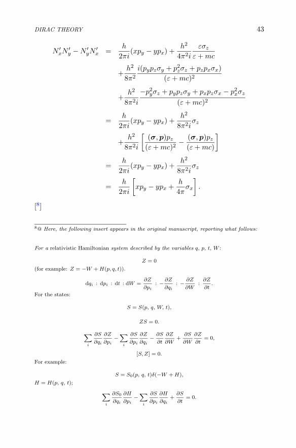
DIRAC THEORY 43

N ′xN ′

y − N ′yN

′x =

h

2πi(xpy − ypx) +

h2

4π2i

εσz

ε + mc

+h2

8π2

i(pypzσy + p2zσz + pzpxσx)

(ε + mc)2

+h2

8π2i

−p2yσz + pypzσy + pxpzσx − p2

xσz

(ε + mc)2

=h

2πi(xpy − ypx) +

h2

8π2iσz

+h2

8π2i

[(σ,p)pz

(ε + mc)2− (σ,p)pz

(ε + mc)

]

=h

2πi(xpy − ypx) +

h2

8π2iσz

=h

2πi

[xpy − ypx +

h

4πσx

].

[8]

8@ Here, the following insert appears in the original manuscript, reporting what follows:

For a relativistic Hamiltonian system described by the variables q, p, t, W :

Z = 0

(for example: Z = −W + H(p, q, t)).

dqi : dpi : dt : dW =∂Z

∂pi: − ∂Z

∂qi: − ∂Z

∂W:

∂Z

∂t.

For the states:

S = S(p, q, W, t),

ZS = 0.

X

i

∂S

∂qi

∂Z

∂pi−X

i

∂S

∂pi

∂Z

∂qi− ∂S

∂t

∂Z

∂W+

∂S

∂W

∂Z

∂t= 0,

[S, Z] = 0.

For example:

S = S0(p, q, t)δ(−W + H),

H = H(p, q, t);

X

i

∂S0

∂qi

∂H

∂pi−X

i

∂S

∂pi

∂H

∂qi+

∂S

∂t= 0.

44 E. MAJORANA: RESEARCH NOTES ON THEORETICAL PHYSICS

1.6.4 Plane-Wave ExpansionFor the Dirac field:

H = H0 + H1, H ′ = H ′0 + H ′

1;

H0 = −cρ1(σ,p) − ρ3mc2, H1 = −eϕ − eρ1(σ,U);

H ′0 = −ρ3cε, ε =

√m2c2 + p2.

ε =√

m2c2 + h2γ2.

ψ = (A,B), ψ′ = (A′, B′):

A(q) =∫

a(γ) e2πi(γ,q)dγ, a(γ) =∫

A(q) e−2πi(γ,q)dq;

B(q) =∫

b(γ) e2πi(γ,q)dγ, b(γ) =∫

B(q) e−2πi(γ,q)dq;

A′(q) =∫

a′(γ) e2πi(γ,q)dγ, a′(γ) =∫

A′(q) e−2πi(γ,q)dq;

B′(q) =∫

b(γ) e2πi(γ,q)dγ, b′(γ) =∫

B′(q) e−2πi(γ,q)dq.

a(γ) =

√ε + mc

2εa′(γ) − h(σ,γ)

√2ε(ε + mc)

b′(γ),

b(γ) =h(σ,γ)

√2ε(ε + mc)

a′(γ) +

√ε + mc

2εb′(γ);

a′(γ) =

√ε + mc

2εa(γ) +

h(σ,γ)√

2ε(ε + mc)b(γ),

b′(γ) = − h(σ,γ)√

2ε(ε + mc)a(γ) +

√ε + mc

2εb(γ).

χ(γ) = (a, b), χ′(γ) = (a′, b′):

χ(γ) =

[√ε + mc

2ε− ihρ2(σ,γ)

√2ε(ε + mc)

]

χ′(γ),

χ′(γ) =

[√ε + mc

2ε+

ihρ2(σ,γ)√

2ε(ε + mc)

]

χ(γ).

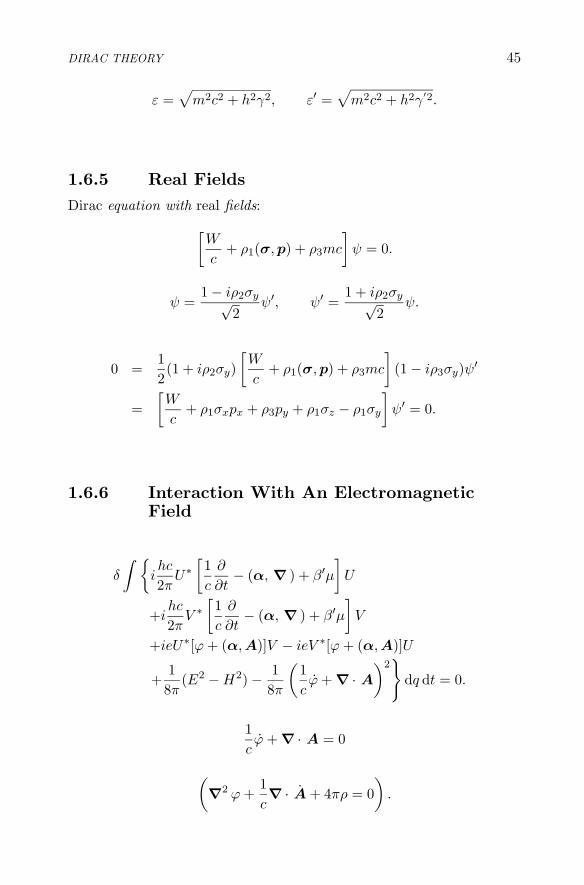
DIRAC THEORY 45

ε =√

m2c2 + h2γ2, ε′ =√

m2c2 + h2γ′2.

1.6.5 Real FieldsDirac equation with real fields:

[W

c+ ρ1(σ,p) + ρ3mc

]ψ = 0.

ψ =1 − iρ2σy√

2ψ′, ψ′ =

1 + iρ2σy√2

ψ.

0 =12(1 + iρ2σy)

[W

c+ ρ1(σ,p) + ρ3mc

](1 − iρ3σy)ψ′

=[W

c+ ρ1σxpx + ρ3py + ρ1σz − ρ1σy

]ψ′ = 0.

1.6.6 Interaction With An ElectromagneticField

δ

∫ {ihc

2πU∗

[1c

∂

∂t− (α, ∇ ) + β′μ

]U

+ihc

2πV ∗

[1c

∂

∂t− (α, ∇ ) + β′μ

]V

+ieU∗[ϕ + (α,A)]V − ieV ∗[ϕ + (α,A)]U

+18π

(E2 − H2) − 18π

(1cϕ + ∇ · A

)2}

dq dt = 0.

1cϕ + ∇ · A = 0

(∇2 ϕ +

1c∇ · A + 4πρ = 0

).

46 E. MAJORANA: RESEARCH NOTES ON THEORETICAL PHYSICS

[1c

∂

∂t− (α, ∇ ) + β′

]U +

2πe

hc[ϕ + (α,A)]V = 0,

[1c

∂

∂t− (α, ∇ ) + β′

]V − 2πe

hc[ϕ + (α,A)]U = 0.

(1c2

∂2

∂t2− ∇2

)ϕ + 4πei(U∗V − V ∗U) = 0,

(1c2

∂

∂t2− ∇2

)A − 4πei(U∗αV − V ∗αV ) = 0.

ρ = −ei(U∗V − V ∗U) = −eψψ − ψ∗ψ

2,

I = ei(U∗αV − V ∗αU) = eψαψ − ψ∗αψ

2

(ψ = U + iV ).

P0 = − 14πc

(1cϕ + ∇ · A

),

Px = − 14πc

Ex,

Py = − 14πc

Ey,

Pz = − 14πc

Ez.

1cϕ + ∇ · A = 0 : P0 = 0;

∇2 ϕ + ∇ · A + 4πρ = 0 : ρ = −c∇ · F

(F = (Px, Py, Pz)).

H =∫ {

ψ[−c(α,p) − βmc2

]ψ − (A, I) + 2πc2P 2 +

18π

|∇×A|2}

dq.

DIRAC THEORY 47

1.7. DIRAC-LIKE EQUATIONS FORPARTICLES WITH SPIN HIGHERTHAN 1/2

By starting from the known Dirac equation for a 4-component spinor, theauthor then wrote down the corresponding equations for 16-component,6-component and 5-component spinors. Explicit expressions for the Diracmatrices for the cases considered were given, thus producing for the firsttime Dirac-like equations for particle with spin higher than 1/2. In thefollowing we report what found in the Quaderno 4 in the same orderas the material appears there; it seems evident, in fact, that the authorhas obtained the reported results just in this order, i.e., not in the moreobvious way from 4-component case to 5-component, to 6-component, to16-component case.

1.7.1 Spin-1/2 Particles (4-Component Spinors)

(W

c+

e

cA0

)→ p0,

(px +

e

cAx

)→ px,

(py +

e

cAy

)→ py,

(pz +

e

cAz

)→ pz.

p0ψ1 + pxψ4 − ipyψ4 + pzψ3 + mc ψ1 = 0,

p0ψ2 + pxψ3 + ipyψ3 − pzψ4 + mc ψ2 = 0,

p0ψ3 + pxψ2 − ipyψ2 + pzψ1 − mc ψ3 = 0,

p0ψ4 + pxψ1 + ipyψ1 + pzψ2 − mc ψ4 = 0.

ψ1 ψ2 ψ3 ψ4

ψ1 p0 + mc 0 pz px − ipy

ψ2 0 p0 + mc px + ipy −pz

ψ3 pz px − ipy p0 − mc 0

ψ4 px + ipy −pz 0 p0 − mc

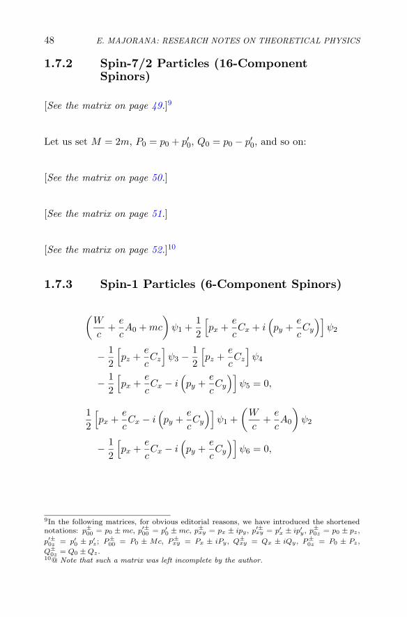
48 E. MAJORANA: RESEARCH NOTES ON THEORETICAL PHYSICS

1.7.2 Spin-7/2 Particles (16-ComponentSpinors)

[See the matrix on page 49.]9

Let us set M = 2m, P0 = p0 + p′0, Q0 = p0 − p′0, and so on:

[See the matrix on page 50.]

[See the matrix on page 51.]

[See the matrix on page 52.]10

1.7.3 Spin-1 Particles (6-Component Spinors)

(W

c+

e

cA0 + mc

)ψ1 +

12

[px +

e

cCx + i

(py +

e

cCy

)]ψ2

− 12

[pz +

e

cCz

]ψ3 −

12

[pz +

e

cCz

]ψ4

− 12

[px +

e

cCx − i

(py +

e

cCy

)]ψ5 = 0,

12

[px +

e

cCx − i

(py +

e

cCy

)]ψ1 +

(W

c+

e

cA0

)ψ2

− 12

[px +

e

cCx − i

(py +

e

cCy

)]ψ6 = 0,

9In the following matrices, for obvious editorial reasons, we have introduced the shortenednotations: p±00 = p0 ± mc, p′±00 = p′0 ± mc, p±xy = px ± ipy , p′±xy = p′x ± ip′y , p±0z = p0 ± pz ,

p′±0z = p′0 ± p′z ; P±00 = P0 ± Mc, P±

xy = Px ± iPy , Q±xy = Qx ± iQy , P±

0z = P0 ± Pz ,

Q±0z = Q0 ± Qz .

10@ Note that such a matrix was left incomplete by the author.

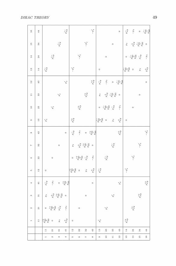
DIRAC THEORY 49

12

34

56

78

910

11

12

13

14

15

16

11

21

31

41

12

22

32

42

13

23

33

43

14

24

34

44

111

p′+ 00

p+ 00

0p

zp− x

y0

p′ z

p′− x

y

221

0p′+ 00

p+ 00

p+ x

y−

pz

0p′ z

p′− x

y

331

pz

p− x

yp′+ 00

p− 00

00

p′ z

p′− x

y

441

p+ x

y−

pz

0p′+ 00

p− 00

0p′ z

p′− x

y

512

0p′+ 00

p+ 00

0p

zp− x

yp′+ x

y−

p′ z

622

00

p′+ 00

p+ 00

p+ x

y−

pz

p′+ x

y−

p′ z

732

0p

zp− x

yp′+ 00

p− 00

0p′+ x

y−

p′ z

842

0p+ x

y−

pz

0p′+ 00

p− 00

p′+ x

y−

p′ z

913

p′ z

p′− x

yp′− 00

p+ 00

0p

zp− x

y0

10

23

p′ z

p′− x

y0

p′− 00

p+ 00

p+ x

y−

pz

0

11

33

p′ z

p′− x

yp

zp− x

yp′− 00

p− 00

00

12

43

p′ z

p′+ x

yp+ x

y−

pz

0p′− 00

p− 00

0

13

14

p′+ x

y−

p′ z

0p′− 00

p+ 00

0p

zp− x

y

14

24

p′+ x

y−

p′ z

00

p′− 00

p+ 00

p+ x

y−

pz

15

34

p′+ x

y−

p′ z

0p

zp− x

yp′− 00

p− 00

0

16

44

p′+ x

y−

p′ z

0p+ x

y−

pz

0p′− 00

p− 00

50 E. MAJORANA: RESEARCH NOTES ON THEORETICAL PHYSICS

11

22

33

44

21

+12

√2

31

+13

√2

41

+14

√2

32

+23

√2

42

+24

√2

43

+34

√2

21

−12

√2

31

−13

√2

41

−14

√2

32

−23

√2

42

−24

√2

43

+34

√2

11

P+ 00

00

00

Pz

√2

P− xy

√2

00

00

Qz

√2

Q− x

y√

20

00

22

0P

+ 00

00

00

0P

+ xy

√2

Pz

√2

00

00

Q+ x

y√

2−

Qz

√2

0

33

00

P− 00

00

Pz

√2

0P

− xy

√2

00

0Q

z√

20

Q− x

y√

20

0

44

00

0P

− 00

00

P+ xy

√2

0P

z√

20

00

Q+ x

y√

20

−Q

z√

20

21

+12

√2

00

00

P+ 00

P+ xy

2−

Pz 2

Pz 2

P− xy

20

0Q

+ xy

2−

Qz 2

Qz 2

Q+ x

y

20

31

+13

√2

Pz

√2

0P

z√

20

P− xy

2P0

00

0P

− xy

2

Q− x

y

20

00

0Q

− xy

241

+14

√2

P+ xy

√2

00

P− xy

√2

−P

z 20

P0

00

Pz 2

−Q

z 20

00

0−

Qz 2

32

+23

√2

0P

− xy

√2

P+ xy

√2

0P

z 20

0P0

0−

Pz 2

−Q

z 20

00

0−

Qz 2

42

+24

√2

0−

Pz

√2

0P

z√

2

P+ xy

20

00

P0

P+ xy

2−

Q+ x

y

20

00

0−

Q+ x

y

243

+34

√2

00

00

0P

+ xy

2

Pz 2

−P

z 2

P− xy

2P

− 00

0−

Q+ x

y

2−

Qz 2

Qz 2

−Q

− xy

20

21

−12

√2

00

00

0Q

+ xy

2−

Qz 2

−Q

z 2−

Q− x

y

20

P+ 00

P+ xy

2−

Pz 2

−P

z 2−

P+ xy

20

31

−13

√2

Qz

√2

0Q

z√

20

Q− x

y

20

00

0−

Q− x

y

2

P− xy

2P0

00

0−

P− xy

241

−14

√2

Q+ x

y√

20

0Q

− xy

√2

−Q

z 20

00

0−

Qz 2

−P

z 20

P0

00

Pz 2

32

−23

√2

0Q

− xy

√2

Q+ x

y√

20

Qz 2

00

00

Qz 2

−P

z 20

0P0

0P

z 242

−24

√2

0−

Qz

√2

0Q

z√

2

Q+ x

y

20

00

0−

Q+ x

y

2−

P+ xy

20

00

P0

P+ xy

243

−34

√2

00

00

0Q

+ xy

2−

Qz 2

−Q

z 2−

Q− x

y

20

0−

P+ xy

2

Pz 2

Pz 2

P− xy

2P

− 00

DIRAC THEORY 51

11

21

31

41

12

22

32

42

13

23

33

43

14

24

34

44

11

0 00

p− 0

z−

p− x

y0

p′− 0

z−

p′− x

y

21

00 0

−p+ x

yp+ 0

z0

p′− 0

z−

p′− x

y

31

p+ 0

zp− x

y0 0

00

p′− 0

z−

p′− x

y

41

p+ x

yp− 0

z0

0 00

p′− 0

z−

p′− x

y

12

00 0

0p− 0

z−

p− x

y−

p′+ x

yp+ 0

z

22

00

0 0−

p+ x

yp+ 0

z−

p′+ x

yp′+ 0

z

32

0p+ 0

zp− x

y0 0

0−

p′+ x

yp′+ 0

z

42

0p+ x

yp− 0

z0

0 0−

p′+ x

yp′+ 0

z

13

p′+ 0

zp′− x

y0 0

0p− 0

z−

p− x

y0

23

p′+ 0

zp′− x

y0

0 0−

p+ x

yp+ 0

z0

33

p′+ 0

zp′− x

yp+ 0

zp− x

y0 0

00

43

p′+ 0

zp′− x

yp+ x

yp− 0

z0

0 00

14

p′+ x

yp′− 0

z0

0 00

p− 0

z−

p− x

y

24

p′+ x

yp′− 0

z0

00 0

−p+ x

yp+ 0

z

34

p′+ x

yp′− 0

z0

p+ 0

zp− x

y0 0

0

44

p′+ x

yp′− 0

z0

p+ x

yp− 0

z0

0 0

52 E. MAJORANA: RESEARCH NOTES ON THEORETICAL PHYSICS

11

22

33

44

21

+12

√2

31

+13

√2

41

+14

√2

32

+23

√2

42

+24

√2

43

+34

√2

21

−12

√2

31

−13

√2

41

−14

√2

32

−23

√2

42

−24

√2

43

+34

√2

11

00

00

0P

− 0z

√2

P− xy

√2

00

00

Q− 0

z√

2−

Q− x

y√

20

00

22

00

00

00

0P

+ xy

√2

P+ 0z

√2

00

00

−Q

+ xy

√2

Q+ 0

z√

20

33

00

00

0P

+ 0z

√2

0P

− xy

√2

00

0−

Q+ 0

z√

20

Q− x

y√

20

0

44

00

00

21

+12

√2

00

0

31

+13

√2

P+ 0z

√2

0P

− 0z

√2

41

+14

√2

P+ xy

√2

00

32

+23

√2

0P

− xy

√2

P+ xy

√2

42

+24

√2

0P

− 0z

√2

0

43

+34

√2

00

0

21

−12

√2

00

00

0−

Q+ x

y

2

Q+ 0

z

2−

Q− 0

z

2

Q− x

y

20

0−

P+ xy

2

P+ 0z

2−

P− 0z

2

P− xy

20

31

−13

√2

Q+ 0

z√

20

−Q

− 0z

√2

Q− x

y

20

00

0−

Q− x

y

2

P− xy

20

00

0P

− xy

241

−14

√2

Q+ x

y√

20

0Q

− 0z

20

00

0−

Q+ 0

z

2

P− 0z

20

00

0P

− 0z

232

−23

√2

0Q

− xy

√2

−Q

+ xy

√2

0Q

+ 0z

20

00

0−

Q+ 0

z

2−

P+ 0z

20

00

0−

P+ 0z

242

−24

√2

0Q

+ 0z

√2

0−

Q+ 0

z√

2

Q+ x

y

20

00

0Q

+ xy

2−

P+ xy

20

00

0−

P+ xy

243

−34

√2

00

00

0Q

+ xy

2−

Q+ 0

z

2

Q− 0

z

2−

Q− x

y

20

−P

+ xy

2

P+ 0z

2−

P− 0z

2

P− xy

20

DIRAC THEORY 53

−12

[pz +

e

cCz

]ψ1 +

(W

c+

e

cA0

)ψ3 +

12

[pz +

e

cCz

]ψ6 = 0,

−12

[pz +

e

cCz

]ψ1 +

(W

c+

e

cA0

)ψ4 +

12

[pz +

e

cCz

]ψ6 = 0,

−12

[px +

e

cCx + i

(py +

e

cCy

)]ψ1 +

(W

c+

e

cA0

)ψ5

+12

[px +

e

cCx + i

(py +

e

cCy

)]ψ6 = 0,

−12

[px +

e

cCx + i

(py +

e

cCy

)]ψ2 +

12

[pz +

e

cCz

]ψ3

+12

[pz +

e

cCz

]ψ4 +

12

[px +

e

cCx − i

(py +

e

cCy

)]ψ5

+(

W

c+

e

cA0 − mc

)= 0.

——————–

In first approximation, for Cx = Cy = Cz = 0:

ψ1 = 0, ψ2 =px − ipy

2mcψ6, ψ3 = − pz

2mcψ6,

ψ4 = − pz

2mcψ6; ψ5 = −px + ipy

2mcψ6;

{

−p2

x + p2y + p2

z

2mc+

W

c+

e

cA0 − mc

}

ψ6 = 0,

W = mc − eA0 +p2

z + p2y + p2

z

2m.

——————–

(W

c+

e

cA0

)+ αx

(px +

e

cCx

)+ αy

(py +

e

cCy

)

+αz

(pz +

e

cCz

)+ βmc = 0;

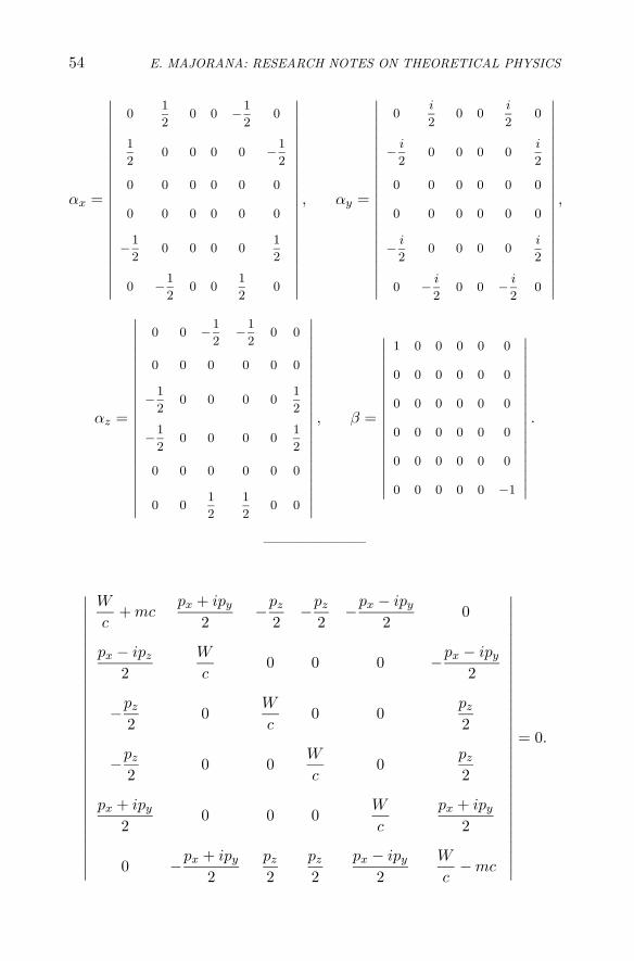
54 E. MAJORANA: RESEARCH NOTES ON THEORETICAL PHYSICS

αx =

∣∣∣∣∣∣∣∣∣∣∣∣∣∣∣∣∣∣∣∣∣

01

20 0 −1

20

1

20 0 0 0 −1

2

0 0 0 0 0 0

0 0 0 0 0 0

−1

20 0 0 0

1

2

0 −1

20 0

1

20

∣∣∣∣∣∣∣∣∣∣∣∣∣∣∣∣∣∣∣∣∣

, αy =

∣∣∣∣∣∣∣∣∣∣∣∣∣∣∣∣∣∣∣∣∣

0i

20 0

i

20

− i

20 0 0 0

i

2

0 0 0 0 0 0

0 0 0 0 0 0

− i

20 0 0 0

i

2

0 − i

20 0 − i

20

∣∣∣∣∣∣∣∣∣∣∣∣∣∣∣∣∣∣∣∣∣

,

αz =

∣∣∣∣∣∣∣∣∣∣∣∣∣∣∣∣∣∣∣∣∣

0 0 −1

2−1

20 0

0 0 0 0 0 0

−1

20 0 0 0

1

2

−1

20 0 0 0

1

2

0 0 0 0 0 0

0 01

2

1

20 0

∣∣∣∣∣∣∣∣∣∣∣∣∣∣∣∣∣∣∣∣∣

, β =

∣∣∣∣∣∣∣∣∣∣∣∣∣∣∣∣∣

1 0 0 0 0 0

0 0 0 0 0 0

0 0 0 0 0 0

0 0 0 0 0 0

0 0 0 0 0 0

0 0 0 0 0 −1

∣∣∣∣∣∣∣∣∣∣∣∣∣∣∣∣∣

.

——————–

∣∣∣∣∣∣∣∣∣∣∣∣∣∣∣∣∣∣∣∣∣∣∣∣∣∣∣∣∣∣

W

c+ mc

px + ipy

2−pz

2−pz

2−px − ipy

20

px − ipz

2W

c0 0 0 −px − ipy

2

−pz

20

W

c0 0

pz

2

−pz

20 0

W

c0

pz

2

px + ipy

20 0 0

W

c

px + ipy

2

0 −px + ipy

2pz

2pz

2px − ipy

2W

c− mc

∣∣∣∣∣∣∣∣∣∣∣∣∣∣∣∣∣∣∣∣∣∣∣∣∣∣∣∣∣∣

= 0.

DIRAC THEORY 55

∣∣∣∣∣∣∣∣∣∣∣∣∣∣∣∣∣∣∣∣∣∣∣∣∣∣∣∣∣∣

2W

c0 0 0 0

W

c− mc

0W

c0 0 0 −px − ipy

2

0 0W

c0 0

pz

2

0 0 0W

c0

pz

2

0 0 0 0W

c

px + ipy

2

W

c− mc −px + ipy

2pz

2pz

2p−xy

2W

c− mc

∣∣∣∣∣∣∣∣∣∣∣∣∣∣∣∣∣∣∣∣∣∣∣∣∣∣∣∣∣∣

= 0,

2W 6

c6− 2

W 5

c5mc− W 4

c4(p2

x + p2y + p2

z)−W 4

c4

(W 2

c2− 2Wm + m2c2

)= 0,

W 2

c2− m2c2 −

(p2

x + p2y + p2

z

)= 0.

1.7.4 5-Component Spinors

(W

c+

e

cA0 + mc

)ψ1 +

12

[px +

e

cCx + i

(py +

e

cCy

)]ψ2

− 1√2

[pz +

e

cCz

]ψ3 −

12

[px +

e

cCx − i

(py +

e

cCy

)]ψ4 = 0,

12

[px +

e

cCx − i

(py +

e

cCy

)]ψ1 +

(W

c+

e

cA0

)ψ2

−12

[px +

e

cCx − i

(py +

e

cCy

)]ψ5 = 0,

− 1√2

[pz +

e

cCz

]ψ1 +

(W

c+

e

cA0

)ψ3 +

1√2

[pz +

e

cCz

]ψ5 = 0,

−12

[px +

e

cCx + i

(py +

e

cCy

)]ψ1 +

(W

c+

e

cA0

)ψ4

+12

[px +

e

cCx + i

(py +

e

cCy

)]ψ5 = 0,

56 E. MAJORANA: RESEARCH NOTES ON THEORETICAL PHYSICS

−12

[px +

e

cCx + i

(py +

e

cCy

)]ψ2 +

1√2

[pz +

e

cCz

]ψ3

+12

[px +

e

cCx − i

(py +

e

cCy

)]ψ4 +

(W

c+

e

cA0 − mc

)ψ5 = 0.

(W

c+

e

cA0

)+ αx

(px +

e

cCx

)+ αy

(py +

e

cCy

)

+αz

(pz +

e

cCz

)+ βmc = 0,

αx =

∣∣∣∣∣∣∣∣∣∣∣∣∣∣∣∣∣∣∣

01

20 −1

20

1

20 0 0 −1

2

0 0 0 0 0

−1

20 0 0

1

2

0 −1

20

1

20

∣∣∣∣∣∣∣∣∣∣∣∣∣∣∣∣∣∣∣

, αy =

∣∣∣∣∣∣∣∣∣∣∣∣∣∣∣∣∣∣∣

0i

20

i

20

− i

20 0 0

i

2

0 0 0 0 0

− i

20 0 0

i

2

0 − i

20 − i

20

∣∣∣∣∣∣∣∣∣∣∣∣∣∣∣∣∣∣∣

,

αz =

∣∣∣∣∣∣∣∣∣∣∣∣∣∣∣∣∣∣∣

0 0 − 1√2

0 0

0 0 0 0 0

− 1√2

0 0 01√2

0 0 0 0 0

0 01√2

0 0

∣∣∣∣∣∣∣∣∣∣∣∣∣∣∣∣∣∣∣

, β =

∣∣∣∣∣∣∣∣∣∣∣∣∣∣∣

1 0 0 0 0

0 0 0 0 0

0 0 0 0 0

0 0 0 0 0

0 0 0 0 −1

∣∣∣∣∣∣∣∣∣∣∣∣∣∣∣

.

2

QUANTUM ELECTRODYNAMICS

2.1. BASIC LAGRANGIAN ANDHAMILTONIAN FORMALISM FOR THEELECTROMAGNETIC FIELD

The author studied the dynamics of the electromagnetic field in a la-grangian framework; the Lagrangian density L was deduced from a leastaction principle and, following a canonical formalism, the Hamiltoniandensity H was then obtained.

δ

∫Ldsdt = 0,

1cϕ + ∇ ·A = 0,

L =18π

{− 1

c2ϕ2 + |∇ ϕ|2 +

1c2

(A2x + A2

y + A2z)

− |∇ Ax|2 − |∇ Ay|2 − |∇ Az|2}

.

ϕ, P0 = − 14πc2

ϕ,

Ax, Px =1

4πc2Ax,

Ay, Py =1

4πc2Ay,

Az, Pz =1

4πc2Az,

�ϕ = 0,

�A = 0.

57

58 E. MAJORANA: RESEARCH NOTES ON THEORETICAL PHYSICS

E = −∇ ϕ − 1cA.

H = ∇×A.

H = P0ϕ + PxAx + PyAy + PzAz − L

=18π

{− 1

c2ϕ2 − |∇ ϕ|2 +

1c2

(A2x + A2

y + A2z) + |∇ Ax|2

+ |∇ Ay|2 + |∇ Az|2}

= 2πc2(−P 20 + P 2

x + P 2y + P 2

z )

+18π

(−|∇ ϕ|2 + |∇ Ax|2 + |∇ Ay|2 + |∇ Az|2

),

4πcP0 = ∇ ·A,

1cϕ + ∇ ·A = 0,

∇2 ϕ +1c∇ · A = 0.

∫H ds =

18π

∫ {−(∇ ·A)2 − |∇ ϕ|2 +

1c2

(A2x + A2

y + A2z)

+ |∇ A2x| + |∇ Ay|2 + |∇ Az|2

}ds

=18π

∫ {−(∇ ·A)2 + ϕ∇2 ϕ +

1c2

(A2x + A2

y + A2z)

− A · ∇2 A

}ds.

E = −∇ ϕ − 1cA,

∫E2ds =

∫ {|∇ ϕ|2 +

2c(∇ ϕ) · A +

1c2

(A2x + A2

y + A2z)}

ds

=∫ {

−ϕ∇2 ϕ − 2cϕ∇ · A +

1c2

(A2x + A2

y + A2z)}

ds

=∫ {

ϕ∇2 ϕ +1c2

(A2x + A2

y + A2z)}

ds,

QUANTUM ELECTRODYNAMICS 59

H = ∇×A,∫H2ds =

∫|∇×A|2ds =

∫A · ∇×∇×A ds

=∫ {

A · ∇ (∇ ·A) − A · ∇2 A}

ds

=∫ {

−(∇ ·A)2 − A · ∇2 A}

ds,

[1]

∫H ds =

18π

∫(E2 + H2) ds.

2.2. ANALOGY BETWEEN THEELECTROMAGNETIC FIELD AND THEDIRAC FIELD

In the following pages, the author explored the possibility of describ-ing the electromagnetic field in full analogy with what usually done fora Dirac field. In a three-dimensional formalism, he then introduced awavefunction ψ in terms of the electric and magnetic fields E,H (and,more specifically, in terms of quantities E ± iH), and its dynamics (forfree fields) was developed in close analogy with the Dirac procedure forspin-1/2 fields. Commutation (rather than anticommutation) rules forDirac-like matrices were adopted, and energy eigenvalues and eigenvec-tors were calculated.For further details, see R. Mignani, M. Baldo and E. Recami, Lett.Nuovo Cim. 11 (1974) 568; E. Giannetto, Atti del IX Congresso Nazio-nale di Storia della Fisica, edited by F. Bevilacqua (Milan, 1988) 173;S. Esposito, Found. Phys. 28 (1998) 231.

1@ In the original manuscript, the author pointed out that, from:

1

cϕ + ∇ ·A = 0, �ϕ = 0,

it follows that:

∇2 ϕ +1

c∇ · A = 0.

60 E. MAJORANA: RESEARCH NOTES ON THEORETICAL PHYSICS

4πρ − ∇ ·E = 0, ∇ ·H = 0,

4πI +1c

∂E

∂t= ∇×H, −1

c

∂H

∂t= ∇×E.

ψ1 = E1 − iH1 = Ex − iHx,

ψ2 = E2 − iH2 = Ey − iHy,

ψ3 = E3 − iH3 = Ez − iHz.

∇ ·ψ = ∇ ·E − i∇ ·H = 4πρ. (1)

∇×ψ = ∇×E − i∇×H = −1c

∂H

∂t− 1

c

∂E

∂t− 4πiI

= − i

c

(∂E

∂t− i

∂H

∂t

)− 4πiI,

4πI +1c

∂ψ

∂t= +i∇×ψ. (2)

——————–

The Maxwell equations are given by:

1c

∂ψ

∂t− i∇×ψ + 4πI = 0,

∇ ·ψ − 4πρ = 0.

1c

∂ψ1

∂t− i

∂ψ3

∂y+ i

∂ψ2

∂z+ 4πIx = 0,

1c

∂ψ2

∂t− i

∂ψ1

∂z+ i

∂ψ3

∂x+ 4πIy = 0,

1c

∂ψ3

∂t− i

∂ψ2

∂x+ i

∂ψ1

∂y+ 4πIz = 0,

∂ψ1

∂x+

∂ψ2

∂y+

∂ψ3

∂z− 4πρ = 0.

QUANTUM ELECTRODYNAMICS 61

Without charge:⎧⎪⎪⎪⎪⎪⎪⎪⎪⎪⎪⎪⎪⎪⎪⎨

⎪⎪⎪⎪⎪⎪⎪⎪⎪⎪⎪⎪⎪⎪⎩

W

cψ1 + ipyψ3 − ipzψ2 = 0,

W

cψ2 + ipzψ1 − ipxψ3 = 0,

W

cψ3 + ipxψ2 − ipyψ1 = 0,

pxψ1 + pyψ2 + pzψ3 = 0.

[2](

W

c+ αxpx + αypy + αzpz

)ψ = 0. (3)

αx =

∣∣∣∣∣∣

0 0 00 0 −i0 +i 0

∣∣∣∣∣∣, αy =

∣∣∣∣∣∣

0 0 +i0 0 0−i 0 0

∣∣∣∣∣∣,

αz =

∣∣∣∣∣∣

0 −i 0+i 0 00 0 0

∣∣∣∣∣∣, 1 =

∣∣∣∣∣∣

1 0 00 1 00 0 1

∣∣∣∣∣∣.

[3]

αxαy − αyαx = −iαz,

[αx, αz]− = +iαy,

[αy, αz]− = iαx.

βx = |1 0 0|, βy = |0 1 0|, βz = |0 0 1|.

(βxpx + βypy + βzpz) ψ = 0. (4)

Following the Dirac method, the eigenvalues of the Maxwell equation areobtained from:

2@ The line before the fourth equation means that it is deduced from the previous threeequations.3@ Note that the signs on the RHS of the following two equations were wrong: correctly, wehave αxαy − αyαx = iαz and [αx, αz ]− = −iαy.

62 E. MAJORANA: RESEARCH NOTES ON THEORETICAL PHYSICS

∣∣∣∣∣∣

W/c −ipz ipy

ipz W/c −ipx

−ipy ipx W/c

∣∣∣∣∣∣= 0,

(W

c

)3

− p2 W

c= 0,

W

c=

⎧⎨

⎩

p,−p,

0,

p =√

p2x + p2

y + p2z.

W/c ψ1 ψ2 ψ3

p p2y + p2

z −pxpy − ippz −pxpz + ippy

−p p2y + p2

z −pxpy + ippz −pxpz − ippy

0 px py pz

——————–

For t = 0:

ψ1 = a δ(x − x0)δ′(y − y0)δ′(r − r0),ψ2 = b δ′(x − x0)δ(y − y0)δ′(z − z0),ψ3 = −(a + b) δ′(x − x0)δ′(y − y0)δ(z − z0).

∂ψ1

∂x+

∂ψ2

∂y+

∂ψ3

∂z= 0.

ψ1(x, y, z) =∫

A(x0, y0, z0) δ(x − x0)δ′(y − y0)δ′(z − z0) dx0dy0dz0,

ψ2(x, y, z) =∫

B(x0, y0, z0) δ′(x − x0)δ(y − y0)δ′(z − z0) dx0dy0dz0,

ψ3(x, y, z) =∫−(A + B) δ′(x − x0)δ′(y − y0)δ(z − z0) dx0dy0dz0.

ψ1 =∂2A

∂y∂z, ψ2 =

∂2B

∂z∂x, ψ3 = −∂2(A + B)

∂x∂y;

QUANTUM ELECTRODYNAMICS 63

∂ψ1

∂x=

∂3A

∂x∂y∂z,

∂ψ2

∂y=

∂2B

∂x∂y∂z,

∂ψ3

∂z= −∂2(A + B)

∂x∂y∂z.

——————–

∂′A

∂y∂z= ψ1,

∂A

∂y=∫

ψ1dz + fy,

A = A0 + F1(x, y) + F2(x, z);∂2B

∂z∂x= ψ2,

B = B0 + F3(x, y) + F4(y, z).

ψ3 = −∂2(A + B)∂x∂y

= −∂2(A0 + B0)∂x∂y

+ F (x, y).

By substituting the expressions:

ψ1 =∂2A

∂y∂z, ψ2 =

∂2B

∂z∂x, ψ3 =

∂2C

∂x∂y,

into the Maxwell equations, we get:

1c

∂3A

∂y∂z∂t− i

∂3C

∂x∂2y+ i

∂2B

∂x∂2z= 0,

1c

∂3B

∂z∂x∂t− i

∂3A

∂y∂2z+ i

∂3C

∂y∂2x= 0,

1c

∂3C

∂x∂y∂t− i

∂3B

∂z∂2x+ i

∂3A

∂z∂2y= 0;

∂3(A + B + C)∂x∂y∂z

= 0.

A + B + C = 0.

∂

∂y

(1c

∂2

∂z∂t+ i

∂2

∂x∂y

)A + i

∂

∂x

(∂2

∂2y+

∂2

∂2z

)B = 0,

∂

∂x

(1c

∂2

∂z∂t− i

∂2

∂x∂y

)B − i

∂

∂y

(∂2

∂2x+

∂2

∂2z

)A = 0,

64 E. MAJORANA: RESEARCH NOTES ON THEORETICAL PHYSICS

[∂

∂y

(1c

∂2

∂x∂t− i

∂2

∂y∂z

)A − ∂

∂x

(1c

∂2

∂y∂t+ i

∂2

∂x∂z

)B = 0.

]

——————–

A = −a ei(γ1x+γ2y+γ3z),

B = −b ei(γ1x+γ2y+γ3z),

C = −c ei(γ1x+γ2y+γ3z);

ψ1 = a γ2γ3 ei(γ1x+γ2y+γ3z),

ψ2 = b γ3γ1 ei(γ1x+γ2y+γ3z),

ψ3 = c γ1γ2 ei(γ1x+γ2y+γ3z).

2.3. ELECTROMAGNETIC FIELD: PLANEWAVE OPERATORS

Plane wave expansion of the electromagnetic field was considered in away similar to what is usually done for a Dirac or a Klein-Gordon field.In the second part, the author again introduced a sort of photon wavefield Ψ, in close analogy to the Dirac field for a spin-1/2 particle andin a full Lorentz-invariant formalism. The properties of this field arededuced from general group-theoretic arguments.

ϕ, P0 = − 14πc2

ϕ, ϕ = 4πc2P0;

Ax, Px =1

4πc2Ax, Ax = 4πc2Px;

Ay, Py =1

4πc2Ay, Ay = 4πc2Py;

Az, Pz = − 14πc2

Az, Az = 4πc2Pz;

P0, −ϕ, P0 = − 14π

∇2 ϕ;

Px, −Ax, Px =14π

∇2 Ax;

Py, −Ay, Py =14π

∇2 Ay;

Pz, −Az Pz =14π

∇2 Az.

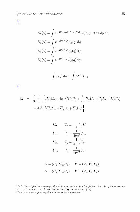
QUANTUM ELECTRODYNAMICS 65

[4]

U0(γ) =∫

e−2πi(γ1x+γ2y+γ3z)ϕ(x, y, z) dxdy dz,

Ux(γ) =∫

e−2πiγ ·qAx(q) dq.

Uy(γ) =∫

e−2πiγ ·qAy(q) dq,

Uz(γ) =∫

e−2πiγ ·qAz(q) dq.

∫L(q) dq =

∫M(γ) dγ,

[5]

M =18π

{− 1

c2U0U0 + 4π2γ2U0U0 +

1c2

(UxUx + UyUy + UzUz)

− 4π2γ2(UxUx + UyUy + U zUz)}

.

U0, V0 = − 14πc2

U0,

Ux, Vx =1

4πc2Ux,

Uy, Vy =1

4πc2Uy,

Uz, Vz =1

4πc2U z.

U = (Ux, Uy, Uz), V = (Vx, Vy, Vz),

U = (Ux, Uy, Uz), V = (Vx, Vy, Vz),

4@ In the original manuscript, the author considered in what follows the role of the operators∇2 = L2 and L =

√∇2. He denoted with q the vector (x, y, z).

5@ A bar over a quantity denotes complex conjugation.

66 E. MAJORANA: RESEARCH NOTES ON THEORETICAL PHYSICS

U0(γ) = U0(−γ),

U0(γ) = U0(−γ),

U(γ) = U(−γ),

U(γ) = U(−γ),

V (γ) = V (−γ),

V (γ) = V (−γ),

V 0(γ) = V0(−γ),

V 0(γ) = V0(−γ).

1c2

U0 + 4π2γ2U0 = 0,

1c2

U + 4π2γ2U = 0,

1cU0 + 2πi(γ1Ux + γ2Uy + γ3Uz) = 0,

2πiγ2U0 +1c(γ1Ux + γ2Uy + γ3Uz) = 0.

[6]

ψ0(γ) =∫

e−2πiγ ·q · 12c√

h

(√2πγc ϕ(q) +

i√2πγc

ϕ(q))

dq,

ψx(γ) =∫

e−2πi(γ ·q · 12c√

h

(√2πγc Ax(q) +

i√2πγc

Ax(q))

dq,

ψy(γ) =∫

e−2πiγ ·q · 12c√

h

(√2πγc Ay(q) +

i√2πγc

Ay(q))

dq,

ψz(γ) =∫

e−2πiγ ·q · 12c√

h

(√2πγc Az(q) +

i√2πγc

Az(q))

dq.

ϕ(q) = c√

h

∫1√

2πγc[ψ0(γ) + ψ0(−γ)] e2πiγ ·qdγ,

ϕ(q) =c√

h

i

∫ √2πγc [ψ0(γ) − ψ0(−γ)] e2πiγ ·qdγ,

6@ Probably, the author proceeded in analogy with the Dirac field .

QUANTUM ELECTRODYNAMICS 67

Ax(q) = c√

h

∫1√

2πγc[ψx(γ) + ψx(−γ)] e2πiγ ·qdγ,

. . . ,

Ax(q) =c√

h

i

∫ √2πγc [ψx(γ) − ψx(−γ)] e2πiγ ·qdγ,

. . . ,

[7]

�ϕ =1c2

ϕ − ∇2 ϕ

=

√h

c i

∫ √2πγc

{ψ0(γ) − ψ0(−γ)

+ 2πγc i ψ0(γ) + 2πγc i ψ0(−γ)}

e2πiγ ·qdγ.

ψ0(γ) = −2πγc i ψ0(γ), ψ0(γ) = 2πγc i ψ0(γ),

ψ(γ) = −2πγc i ψx(γ), ψx(γ) = 2πγc i ψx(γ),. . . .

18π

∫ {− 1

c2ϕ2 − |∇ ϕ|2 +

1c2

(A2x + A2

y + A2z)

+ |∇ Ax|2 + |∇ Ay|2 + |∇ Az|2}

dq

=∫

hγc

{−ψ0(γ)ψ0(γ) + ψ0(γ)ψ0(γ)

2+

ψx(γ)ψx(γ) + ψx(γ)ψx(γ)2

+ψy(γ)ψy(γ) + ψy(γ)ψy(γ)

2+

ψz(γ)ψz(γ) + ψz(γ)ψz(γ)2

}

dγ,

W =∫

hγc{−ψ0(γ)ψ0(γ) + ψx(γ)ψx(γ)

+ ψy(γ)ψy(γ) + ψz(γ)ψz(γ)}

dγ.

7@ In the original manuscript, the author also cited the following (seeming) identity, whosemeaning in this general framework is not clear:

0 = ϕ(q) − ϕ(q)

= c√

h

Z

1√

2πγc

n

ψ0(γ) + ψ0(−γ) + 2πγc i ψ0(q) − 2πγc i ψ0(−γ)o

e2πiγ·qdγ.

68 E. MAJORANA: RESEARCH NOTES ON THEORETICAL PHYSICS

ψ0(γ)ψ0(γ′) − ψ0(γ′)ψ0(γ) = −δ(γ − γ′),

ψx(γ)ψx(γ′) − ψx(γ′)ψx(γ) = +δ(γ − γ′),

. . . .

∇2 ϕ +1c∇ · A =

= c√

h

∫2π

√2πγ

c

{−γ[ψ0(γ) + ψ0(−γ)] + γx[ψx(γ) − ψx(−γ)]

+ γy[ψy(γ) − ψy(−γ)] + γz[ψz(γ) − ψz(−γ)]}

e2πiγ ·qdγ,

1cϕ + ∇ ·A

=ch√

i

∫ √2π

γc

{γ[ψ0(γ) − ψ0(−γ)] − γx[ψx(γ) − ψx(−γ)]

− γy[ψy(γ) − ψy(−γ)] − γz[ψz(γ) − ψz(−γ)]}

e2πiγ ·qdγ,

γψ0 − γxψx − γyψy − γzψz = 0,

γψ0 − γxψx − γyψy − γzψz = 0,

ψ0 = ψ0(γ), ψx = ψx(γ), . . ., ψ0 = ψ0(γ), ψx = ψx(γ), . . ..

2.3.1 Dirac Formalism

Ψ = (ψ0, ψx, ψy, ψz),

H = − h

2πi

∂

∂t, px =

h

2πi

∂

∂x, pz =

h

2πi

∂

∂y, pz =

h

2πi

∂

∂z;

Sx =

∣∣∣∣∣∣∣∣

0 0 0 00 0 0 00 0 0 −10 0 1 0

∣∣∣∣∣∣∣∣

, Sy =

∣∣∣∣∣∣∣∣

0 0 0 00 0 0 10 0 0 00 −1 0 0

∣∣∣∣∣∣∣∣

,

Sz =

∣∣∣∣∣∣∣∣

0 0 0 00 0 −1 00 1 0 00 0 1 0

∣∣∣∣∣∣∣∣

;

QUANTUM ELECTRODYNAMICS 69

Tx =

∣∣∣∣∣∣∣∣

0 1 0 01 0 0 00 0 0 00 0 0 0

∣∣∣∣∣∣∣∣

, Ty =

∣∣∣∣∣∣∣∣

0 0 1 00 0 0 01 0 0 00 0 0 0

∣∣∣∣∣∣∣∣

,

Tz =

∣∣∣∣∣∣∣∣

0 0 0 10 0 0 00 0 0 01 0 0 0

∣∣∣∣∣∣∣∣

.

1) Ψ′ = HΨ = hγcΨ

2) Ψ′ = pxΨ = hγxΨ

3) Ψ′ = pyΨ = hγyΨ

4) Ψ′ = pzΨ = hγzΨ

5) Ψ′ = SxΨ =

⎧⎪⎪⎪⎪⎨

⎪⎪⎪⎪⎩

−γy∂

∂γz+ γz

∂

∂γy+

∣∣∣∣∣∣∣∣∣∣

0 0 0 0

0 0 0 0

0 0 0 −1

0 0 1 0

∣∣∣∣∣∣∣∣∣∣

⎫⎪⎪⎪⎪⎬

⎪⎪⎪⎪⎭

Ψ

6) Ψ′ = SyΨ =

⎧⎪⎪⎪⎪⎨

⎪⎪⎪⎪⎩

−γz∂

∂γz+ γx

∂

∂γz+

∣∣∣∣∣∣∣∣∣∣

0 0 0 0

0 0 0 1

0 0 0 0

0 −1 0 0

∣∣∣∣∣∣∣∣∣∣

⎫⎪⎪⎪⎪⎬

⎪⎪⎪⎪⎭

Ψ

7) Ψ′ = SzΨ =

⎧⎪⎪⎪⎪⎨

⎪⎪⎪⎪⎩

−γx∂

∂γy+ γy

∂

∂γx+

∣∣∣∣∣∣∣∣∣∣

0 0 0 0

0 0 −1 0

0 1 0 0

0 0 0 0

∣∣∣∣∣∣∣∣∣∣

⎫⎪⎪⎪⎪⎬

⎪⎪⎪⎪⎭

Ψ

8) Ψ′ = TxΨ =

⎧⎪⎪⎪⎪⎨

⎪⎪⎪⎪⎩

−γ∂

∂γx− γx

2γ+

∣∣∣∣∣∣∣∣∣∣

0 0 0 0

1 −γx/γ 0 0

0 −γy/γ 0 0

0 −γz/γ 0 0

∣∣∣∣∣∣∣∣∣∣

− 2πi ct γx

⎫⎪⎪⎪⎪⎬

⎪⎪⎪⎪⎭

Ψ

70 E. MAJORANA: RESEARCH NOTES ON THEORETICAL PHYSICS

9) Ψ′ = TyΨ =

⎧⎪⎪⎪⎪⎨

⎪⎪⎪⎪⎩

−γ∂

∂γy− γy

2γ+

∣∣∣∣∣∣∣∣∣∣

0 0 0 0

0 0 −γx/γ 0

1 0 −γy/γ 0

0 0 −γz/γ 0

∣∣∣∣∣∣∣∣∣∣

− 2πi ct γy

⎫⎪⎪⎪⎪⎬

⎪⎪⎪⎪⎭

Ψ

10) Ψ′ = TzΨ =

⎧⎪⎪⎪⎪⎨

⎪⎪⎪⎪⎩

−γ∂

∂γz− γz

2γ+

∣∣∣∣∣∣∣∣∣∣

0 0 0 0

0 0 0 −γx/γ

0 0 0 −γy/γ

1 0 0 −γz/γ

∣∣∣∣∣∣∣∣∣∣

− 2πi ct γz

⎫⎪⎪⎪⎪⎬

⎪⎪⎪⎪⎭

Ψ

ψ0 = 0,Ψ = (ψx, ψy, ψz).

γ = (γx, γy, γz), γ =√

γ2x + γ2

y + γ2z .

(γ′, γ′x, γ′

y, γ′z) = C(γ, γx, γy, γz),

C = ‖cik‖ (i, k = 0, 1, 2, 3)

c200 −

3∑

i=1

c20i = 1,

c00 ci0 −3∑

k=1

c0k cik = 0, (i = 1, 2, 3),

ci0 ck0 −3∑

k=10

cik cki = −∂ik, (i, k = 1, 2, 3).

Ψ′(γ′) = e−2πic(γ′−γ)t

√γ

γ′ D Ψ(γ),

D = ‖dik‖ (i, k = 1, 2, 3)

d11 = c11 −γ′

x

γ′ c01, d21 = c21 −γ′

y

γ′ c01, d31 = c31 −γ′

z

γ′ c01,

d12 = c12 −γ′

x

γ′ c02, d22 = c22 −γ′

y

γ′ c02, d32 = c32 −γ′

z

γ′ c02,

d13 = c13 −γ′

x

γ′ c03, d23 = c23 −γ′

y

γ′ c03, d33 = c33 −γ′

z

γ′ c03.

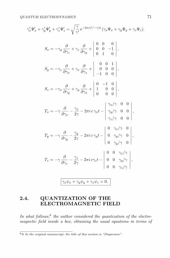
QUANTUM ELECTRODYNAMICS 71

γ′xΨ′

x + γ′yΨ

′y + γ′

zΨ′z =

√γ

γ′ e−2πc(γ′−γ)t (γxΨx + γyΨy + γzΨz).

Sx = −γy∂

∂γz+ γz

∂

∂γy+

∣∣∣∣∣∣

0 0 00 0 −10 1 0

∣∣∣∣∣∣,

Sy = −γz∂

∂γx+ γx

∂

∂γz+

∣∣∣∣∣∣

0 0 10 0 0

−1 0 0

∣∣∣∣∣∣,

Sz = −γx∂

∂γy+ γy

∂

∂γx+

∣∣∣∣∣∣

0 −1 01 0 00 0 0

∣∣∣∣∣∣,

Tx = −γ∂

∂γx− γx

2γ− 2πi c γxt −

∣∣∣∣∣∣∣

γx/γ 0 0

γy/γ 0 0

γz/γ 0 0

∣∣∣∣∣∣∣,

Ty = −γ∂

∂γy− γy

2γ− 2πi c γyt −

∣∣∣∣∣∣∣

0 γx/γ 0

0 γy/γ 0

0 γy/γ 0

∣∣∣∣∣∣∣,

Tz = −γ∂

∂γz− γz

2γ− 2πi cγzt −

∣∣∣∣∣∣∣

0 0 γx/γ

0 0 γy/γ

0 0 γz/γ

∣∣∣∣∣∣∣,

γxψx + γyψy + γzψz = 0.

2.4. QUANTIZATION OF THEELECTROMAGNETIC FIELD

In what follows,8 the author considered the quantization of the electro-magnetic field inside a box, obtaining the usual equations in terms of

8@ In the original manuscript, the title of this section is “Dispersion”.

72 E. MAJORANA: RESEARCH NOTES ON THEORETICAL PHYSICS

oscillators. Particular care was devoted to distinguish the role of theright-handed polarized states from that of the left-handed ones.

∇ ·E = ∇ ·C = 0.

dS = dxdy dz:

18π

∫ (E2 − H2

)dS dt = minimum,

ϕ = 0.

E = −1c

∂C

∂t, H = ∇×C;

δE = −1c

∂

∂tδC, δH = ∇× δC.

1c

∂H

∂t+ ∇×E = 0,

1c

∂E

∂t= ∇×H = ∇×∇×C = ∇ (∇ ·C) − ∇2 C

= −∇2 C.

Conjugate variables:

Cx, Cy, Cz;

− 14πc

Ex, − 14πc

Ey, − 14πc

Ez.

H =18π

∫(E2 + H2) dS.

Let us consider the electromagnetic field confined inside a cube with sidek, its volume being S = k3:

γ1 =n1

k, γ2 =

n2

k, γ3 =

n3

k.

dN = 2k3 dγ1 dγ2 dγ3.

v = cγ.

QUANTUM ELECTRODYNAMICS 73

γ =√

γ21 + γ2

2 + γ23 =

v

c.

A1s = k1 cos 2π(γ1x + γ2y + γ3z) + k2 sin 2π(γ1x + γ2y + γ3z),

A2s = −k1 sin 2π(γ1x + γ2y + γ3z) + k2 cos 2π(γ1x + γ2y + γ3z),

A3s = k1 cos 2π(γ1x + γ2y + γ3z) − k2 sin 2π(γ1x + γ2y + γ3z),

A4s = k1 sin 2π(γ1x + γ2y + γ3z) + k2 cos 2π(γ1x + γ2y + γ3z);

A1s and A2

s correspond to right-handed, circularly polarized waves, whileA3

s and A4s correspond to the left-handed ones.

The direction of s = (v1, v2, v3) is defined by the right-handed directionof k1, k2. Note that γ1, γ2, γ3 are given apart from a simultaneous changeof sign!

s −→ −s,k1, k2 −→ k2, k1.

A1−s = A2

s,

A2−s = A1

s,

A3−s = A4

s,

A4−s = A3

s.

|k1| = 1, |k2| = 1; S = k3.

C =∑

aisA

is,

E =∑

bisA

is.

Notice that, in these sums, the terms corresponding to s and those cor-responding to −s give the same contribution: s ≡ −s. The terms with sand −s are counted only once; the sign of s is defined by the right-handedrotation of k1,k2 !

74 E. MAJORANA: RESEARCH NOTES ON THEORETICAL PHYSICS

aisb

is − bi

sais =

2hc

iS.

bis = −1

cai

s, ais =

14πγ2c

bis.

ais + 4π2γ2c2ai

s = 0, bis + 4π2γ2c2bi

s = 0,

γ2c2 = ν2.

ais = −cbi

s,

bis = 4π2γ2c ai

s.

H =∑

s,i

4π2γ2ai2s + bi2

s

8πS.

ais = −4πc

S

∂H

∂bis

, bis =

4πc

S

∂H

∂ais

.

pis =

√νSπ

hcai

s, qis =

√S

4πνhcbis,

ais =

√hc

νSπpi

s, bis =

√4πνhc

Sqis.

H =∑

ν,i

12(pi2

s + qi2s )hν.

pisq

is − qi

spis =

1i, ai

sbis − bi

sais =

2hc

iS.

pis = −2πνqi

s = −2π

h

∂H

∂qis

, qis = 2πνpi

s =2π

h

∂H

∂pis

.

QUANTUM ELECTRODYNAMICS 75

s → pRs =

p′s − q2s√

2, qR

s =q′s + p′s√

2, pR

s qRs − qR

s pRs =

1i;

−s → PR−s =

p2s − q′s√

2, qR

−s =q2s + p′s√

2, pR

−sqR−s − qR

−spR−s =

1i;

s → pLs =

p4s − q3

s√2

, qLs =

q4s + p3

s√2

, pLs qL

s − qLs pL

s =1i;

−s → pL−s =

p3s − q4

s√2

, qL−s =

q3s + p4

s√2

, pL−sq

L−s − qL

−spL−s =

1i.

From now on, the terms with s are distinct from those with −s !

pRs qR

s − qRs pR

s =1i, pL

s qLs − qL

s pLs =

1i.

as =pR

s − iqRs√

2bs =

pLs − iqL

s√2

a�s =

pRs + iqR

s√2

b�s =

pLs + iqL

s√2

asa�s − a�

sas = 1 bsb�s − b�

sbs = 1

a�sas =

12(pD 2

s + qD 2s ) − 1

2b�sbs =

12(pS 2

s + qS 2s ) − 1

2

a�sas = ns, (ns = 0, 1, 2, . . .) b�

sbs = n′s

as(ns, ns + 1) =√

ns + 1 bs(n′s, n

′s + 1) =

√n′

s + 1

a�s(ns, ns − 1) =

√ns bs(n′

s, n′s−1) =

√n′

s

pRs =

as + a�s√

2, pL

s =bs + b�

s√2

;

qRs = i

as − a�s√

2, qL

s = ibs + b�

s√2

.

76 E. MAJORANA: RESEARCH NOTES ON THEORETICAL PHYSICS

W =12

∑

s,i

12hνs(pi 2

s + qi 2s )

=∑

s

12hνs(pD 2

s + qD 2s ) +

∑

s

12hνs(pS 2

s + qS 2s )

=∑

s

hνs(ns + n′s) (+ an infinite constant).

p1s =

pRs + qR

−s√2

, q1s =

qRs − pR

−s√2

,

p2s =

pR−s + qR

s√2

, q2s =

qR−s − pR

s√2

,

p3s =

pL−s + qL

s√2

, q3s =

qL−s − pL

s√2

,

p4s =

pL−s + qL

−s√2

, q4s =

qLs − pL

−s√2

(in the LHS s and −s are gathered together, while on the RHS they arekept distinct).

p1s =

12[as + ia−s + a�

s − ia�−s], q1

s =12[ias − a−s − ia�

s − a�−s],

p2s =

12[a−s + ias + a�

−s − ia�s], q2

s =12[ias − as − ia�

s − a�s],

p3s =

12[b−s + ibs + b�

−s − ib�s], q3

s =12[ib−s − bs − ib�

−s − b�s],

p4s =

12[bs + ib−s + b�

s − ib�s], q4

s =12[ibs − b−s − ib�

s − b�−s].

as = . . . , bs = . . . , a∗s = . . . , b∗s = . . . .

In what follows, the orthogonal functions Ais are defined for all the values

of s (see page 73); the indices of k1, k2 are given in such a way that thevectors k1, k2, s form a right-handed trihedron. The vectors k1 and k2

transform one into the other by changing s into −s. Each function Ais

is counted twice, due to the relations:

A1s = A2

−s, A2s = A1

−s, A3s = A4

−s, A4s = A3

−s.

QUANTUM ELECTRODYNAMICS 77

C =c

2

√h

πS

∑

s

1√

νs[(as + a�

s)A1s + i(as − a�

s)A2s

+ i(bs − b�s)A

3s + (bs + b�

s)A4s],

E =

√πh

S

∑

s

√νs [i(as − a�

s)A1s − (as + a�

s)A2s

− (bs + b�s)A

3s + i(bs − b�

s)A4s].

as(ns, ns+1) =√

ns + 1, bs(n′s, n

′s+1) =

√n′

s + 1,

a�s(ns, ns−1) =

√ns, bs(n′

s, n′s−1) =

√n′

s,asa

�s − a�

sas = 1, bsb�s − b�

sbs = 1,a�

sas = ns, b�sbs = n′

s.

W =14

∑

s

hνs[� a2s+ � a∗2s + asa

∗s + a∗sas−� a2

s−� a∗2s + asa∗s + a∗sas

−� b2s−� b∗2s + bsb

∗s + b∗sbs+ � b2

s+ � b∗2s + bsb∗s + b∗sbs]

=∑

s

hνs(ns + n′s+1) =

∑

s

hνs(ns + Ns) + an infinite constant,

with:

ns = a∗sas,

Ns = b∗sbs.

By absorbing the infinite constant into W , we have:

WR =∑

s

hνs(ns + Ns).

We have used Ns instead of n′s: ns corresponds to right-handed polarized

waves, while Ns to the left-handed ones.

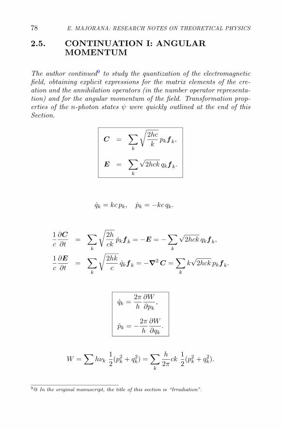
78 E. MAJORANA: RESEARCH NOTES ON THEORETICAL PHYSICS

2.5. CONTINUATION I: ANGULARMOMENTUM

The author continued9 to study the quantization of the electromagneticfield, obtaining explicit expressions for the matrix elements of the cre-ation and the annihilation operators (in the number operator representa-tion) and for the angular momentum of the field. Transformation prop-erties of the n-photon states ψ were quickly outlined at the end of thisSection.

C =∑

k

√2hc

kpkfk,

E =∑

k

√2hck qkfk.

qk = kc pk, pk = −kc qk.

1c

∂C

∂t=

∑

k

√2h

ckpkfk = −E = −

∑

k

√2hck qkfk,

1c

∂E

∂t=

∑

k

√2hk

cqkfk = −∇2 C =

∑

k

k√

2hck pkfk.

qk =2π

h

∂W

∂pk,

pk = −2π

h

∂W

∂qk.

W =∑

hνk12(p2

k + q2k) =

∑

k

h

2πck

12(p2

k + q2k).

9@ In the original manuscript, the title of this section is “Irradiation”.

QUANTUM ELECTRODYNAMICS 79

qk = −2πi

h(qkW − Wqk),

pk = −2πi

h(pkW − Wqk);

i(qkW − Wqk) =∂W

∂pk,

−i(pkW − Wpk) =∂W

∂qk;

−i(qkpk − pkqk) = 1,

+i(pkqk − qkpk) = 1.

pkqk − qkpk =1i.

W =∑

k

hνk

(nk +

12

)=∑

hνkp2

k + q2k

2.

12(p2

k + q2k) =

pk + iqk√2

pk − iqk√2

+12,

ak =pk − iqk√

2, a∗k =

pk + iqk√2

.

aka∗k − a∗kak =

i

2(pkqk − qkpk + pkqk − qkpk) = 1.

a∗kak = nk,aka

∗k = nk + 1.

ak =pk − iqk√

i, pk =

ak + a∗k√2

,

a∗k =pk + iqk√

i, qk =

a∗k − ak

i√

2.

80 E. MAJORANA: RESEARCH NOTES ON THEORETICAL PHYSICS

ak =

∣∣∣∣∣∣∣∣∣∣∣∣

0 1 0 0 0 0 . . .

0 0√

2 0 0 0 . . .

0 0 0√

3 0 0 . . .

0 0 0 0√

4 0 . . .

0 0 0 0 0√

5 . . .. . . . . . . . . . . . . . . . . . . . .

∣∣∣∣∣∣∣∣∣∣∣∣

,

a∗k =

∣∣∣∣∣∣∣∣∣∣∣∣∣∣

0 0 0 0 0 0 . . .1 0 0 0 0 0 . . .

0√

2 0 0 0 0 . . .

0 0√

3 0 0 0 . . .

0 0 0√

4 0 0 . . .

0 0 0 0√

5 0 . . .. . . . . . . . . . . . . . . . . . . . .

∣∣∣∣∣∣∣∣∣∣∣∣∣∣

;

a∗kak =

∣∣∣∣∣∣∣∣∣∣

0 0 0 0 . . .0 1 0 0 . . .0 0 2 0 . . .0 0 0 3 . . .

. . . . . . . . . . . . . . .

∣∣∣∣∣∣∣∣∣∣

,

aka∗k =

∣∣∣∣∣∣∣∣∣∣

1 0 0 0 . . .0 2 0 0 . . .0 0 3 0 . . .0 0 0 4 . . .

. . . . . . . . . . . . . . .

∣∣∣∣∣∣∣∣∣∣

;

pk =

∣∣∣∣∣∣∣∣

0 1/√

2 0 . . .

1/√

2 0 1 . . .0 1 0 . . .

. . . . . . . . . . . .

∣∣∣∣∣∣∣∣

,

qk =

∣∣∣∣∣∣∣∣

0 i/√

2 0 . . .

−i/√

2 0 −i . . .0 i 0 . . .

. . . . . . . . . . . .

∣∣∣∣∣∣∣∣

.

C ′ = C + ε S C, E′ = E + ε S E.

p′r = pr + ε∑

s

Srsps, q′r = qr + ε∑

s

Srsqs.

Srs = −Ssr.

QUANTUM ELECTRODYNAMICS 81

ψ = ψ(n1, n2, . . .),

ψ′ = ψ +T

iεψ;

q′ = q +ε

i(qT − Tq),

p′ = p +ε

i(pT − Tp).

prT − Tpr = i∑

Srsps,

qrT − Tqr = i∑

Srsqs.

T =∑

rs

Srs prqs.

T is the angular momentum in units h/2π.

T =∑

Srsprqs =∑

r<s

Srs(prqs − psqr).

prqs − psqr =12i

(a∗ra∗s − aras − a∗ras + ara

∗s

− a∗sa∗r − asar + a∗sar − asa

∗r)

=1i(ara

∗s − asa

∗r).

T =∑

r<s

1i(ara

∗s − asa

∗r)Srs.

For n photons:

ψ = ψ(n1, n2, . . .) δ(∑

ni − n)

.

For n = 1, ψ = ψ(n1, n2, . . .) and all ni but one vanish, and the non-zeronumber is equal to 1:

ψ(1, 0, 0, 0, 0, . . .) = c1,

ψ(0, 1, 0, 0, 0, . . .) = c2,

ψ(0, 0, 1, 0, 0, . . .) = c3,

. . . .

82 E. MAJORANA: RESEARCH NOTES ON THEORETICAL PHYSICS

ψ = (c1, c2, c3, . . .).

ψ′ = Tψ.

∑

r<s

Srs(ara∗s − asa

∗r) =

∑

r,s

Srsara∗s,

1i

∑

rs

Srsara∗sψ = (c′1, c

′2, . . .).

c′s =1i

∑Srscr = i

∑Ssrcr.

c′r = i∑

Srscs.

2.6. CONTINUATION II: INCLUDING THEMATTER FIELDS

What had been studied in the Sect. 2.4 was tentatively generalized hereto the case of an electromagnetic field interacting with a charged Diracfield ψ. As above, the scalar potential is assumed to be zero, ϕ = 0, andagain the box volume is S = k3.

Dirac equations:[W

c+ ρ3 σ ·

(p +

e

cC)

+ ρ1mc

]ψ = 0.

p = (px, py, pz). For plane waves, px, py, pz are constant.

ψrp = (ψ1, ψ2, ψ3, ψ4) = e(2πi/h)(pxx+pyy+pzz)(ε1, ε2, ε3, ε4),

W

c=

⎧⎨

⎩

+√

m2c2 + p2, for r = 1, 2,

−√

m2c2 + p2, for r = 3, 4.

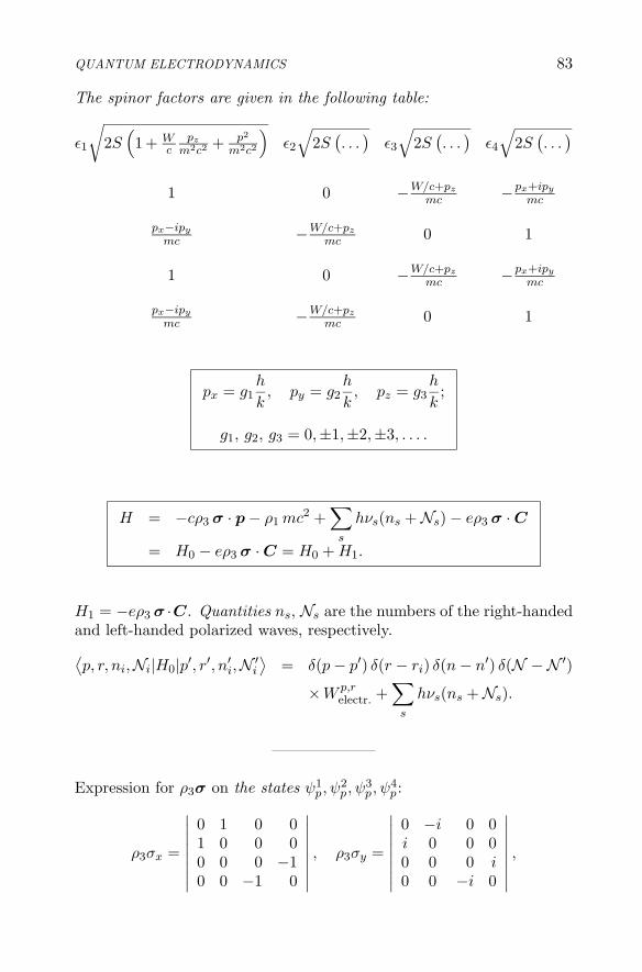
QUANTUM ELECTRODYNAMICS 83

The spinor factors are given in the following table:

ε1

√2S

(1 + W

cpz

m2c2+ p2

m2c2

)ε2

√2S

(. . .

)ε3

√2S

(. . .

)ε4

√2S

(. . .

)

1 0 −W/c+pz

mc −px+ipy

mc

px−ipy

mc −W/c+pz

mc 0 1

1 0 −W/c+pz

mc −px+ipy

mc

px−ipy

mc −W/c+pz

mc 0 1

px = g1h

k, py = g2

h

k, pz = g3

h

k;

g1, g2, g3 = 0,±1,±2,±3, . . . .

H = −cρ3 σ · p − ρ1 mc2 +∑

s

hνs(ns + Ns) − eρ3 σ · C

= H0 − eρ3 σ · C = H0 + H1.

H1 = −eρ3 σ ·C. Quantities ns, Ns are the numbers of the right-handedand left-handed polarized waves, respectively.⟨p, r, ni,Ni|H0|p′, r′, n′

i,N ′i

⟩= δ(p − p′) δ(r − ri) δ(n − n′) δ(N −N ′)

×W p,relectr. +

∑

s

hνs(ns + Ns).

——————–

Expression for ρ3σ on the states ψ1p, ψ

2p, ψ

3p, ψ

4p:

ρ3σx =

∣∣∣∣∣∣∣∣

0 1 0 01 0 0 00 0 0 −10 0 −1 0

∣∣∣∣∣∣∣∣

, ρ3σy =

∣∣∣∣∣∣∣∣

0 −i 0 0i 0 0 00 0 0 i0 0 −i 0

∣∣∣∣∣∣∣∣

,

84 E. MAJORANA: RESEARCH NOTES ON THEORETICAL PHYSICS

ρ3σz =

∣∣∣∣∣∣∣∣

1 0 0 00 −1 0 00 0 −1 00 0 0 1

∣∣∣∣∣∣∣∣

.

ψ1p = (1, 0, 0, 0) e(2πi/h)(pxx+pyy+pzz),

ψ2p = (0, 1, 0, 0) e(2πi/h)(pxx+pyy+pzz),

ψ3p = (0, 0, 1, 0) e(2πi/h)(pxx+pyy+pzz),

ψ4p = (0, 0, 0, 1) e(2πi/h)(pxx+pyy+pzr).

2.7. QUANTUM DYNAMICS OFELECTRONS INTERACTING WITH ANELECTROMAGNETIC FIELD

The dynamics of a system composed of interacting electrons and pho-tons is considered in the realm of Quantum Field Theory (Klein-Gordontheory). The electrons are described by a field ψ (or P , deduced fromψ), while the electromagnetic field is described in terms of the potential(ϕ,C). An expression for the quantized Hamiltonian is given, along withthe commutation rules for creation/annihilation operators.For a charge −e we have:

[(− h

2πic

∂

∂t+

e

cϕ

)2

−∑

x

(h

2πi

∂

∂x+

e

cCx

)2

− m2c2

]

ψ = 0.

P =h2

8π2c2m

(∂

∂t+

2πi

heϕ

)ψ,

P =h2

8π2c2m

(∂

∂t− 2πi

heϕ

)ψ.

[1c2

(∂

∂t− 2πi

heϕ

)2

−∑

x

(∂

∂x+

2πi

hceCx

)2

+4π2

h2m2c2

]

ψ = 0,

[1c2

(∂

∂t+

2πi

heϕ

)2

−∑

x

(∂

∂x− 2πi

hceCx

)2

+4π2

h2m2c2

]

ψ = 0.

∇2 Cx − ∂

∂x∇ ·C =

∂Cx

∂y2+

∂2Cx

∂r2− ∂2Cy

∂x∂y− ∂2Cz

∂x∂z.

QUANTUM ELECTRODYNAMICS 85[

h2

8π2mc2

(∂

∂t− 2πi

heϕ

)2

− h2

8π2m

∑

x

(∂

∂x+

2πi

hceCx

)2

+12mc2

]

ψ = 0,

(1)

[h2

8π2mc2

(∂

∂t+

2πi

heϕ

)2

− h2

8π2m

∑

x

(∂

∂x− 2πi

hceCx

)2

+12mc2

]

ψ = 0.

(2)

(∂

∂t− 2πi

heϕ

)P = −1

2mc2ψ +

h2

8π2m

∑

x

(∂

∂x+

2πi

hceCx

)2

ψ, (3)

(∂

∂t+

2πi

heϕ

)P = −1

2mc2ψ +

h2

8π2m

∑

x

(∂

∂x− 2πi

hceCx

)ψ, (4)

(∂

∂t+

2πi

heϕ

)ψ =

8π2mc2

h2P, (5)

(∂

∂t− 2πi

heϕ

)ψ =

8π2mc2

h2P . (6)

ρ =he

4πimc2

[ψ

(∂

∂t− 2πi

hceϕ

)ψ − ψ

(∂

∂t+

2πi

hceϕ

)ψ

],

ix = − he

4πimc

[ψ

(∂

∂x+

2πi

hceϕ

)ψ − ψ

(∂

∂x− 2πi

hcdx

)ψ

],

. . . .

——————–

dτ = dV dt.

[10]

10@ Notice that, more appropriately, one should write d4τ = d3V dt, since dτ denotes the4-dimensional volume element, while drmV is the 3-dimensional space volume element.

86 E. MAJORANA: RESEARCH NOTES ON THEORETICAL PHYSICS

δ

∫ {h2

8π2m

[1c2

(∂

∂t+

2πi

heϕ

)ψ

(∂

∂t− 2πi

heϕ

)ψ

−∑

x

(∂

∂x− 2πix

hceCx

)ψ ·

(∂

∂x+

2πi

hceCx

)ψ

]

− 12mc2ψψ +

18π

(∣∣∣∣1c

∂C

∂t+ ∇ ϕ

∣∣∣∣

2

− |∇×C|2)}

dτ = 0.

(7)

From this, the variation with respect to ψ or ψ gives Eq. (1) or (2),respectively. The variation with respect to ϕ yields:

− 14π

∑

x

∂

∂x

(∂ϕ

∂x+

1c

∂C

∂t

)

− he

4πimc2

[ψ

(∂

∂t− 2πi

heϕ

)ψ − ψ

(∂

∂t+

2πi

heϕ

)ψ

]= 0,

14π

∇ ·E − ρ = 0. (8)

The variation with respect to Cx instead gives:

− 14πc

∂

∂t

(∂ϕ

∂x+

1c

∂Cx

∂t

)− 1

4π

[∂

∂y

(∂Cy

∂x− ∂Cx

∂y

)

− ∂

∂z

(∂Cx

∂z− ∂Cz

∂x

)]− he

4πimc

[ψ

(∂

∂x+

2πi

hceCx

)ψ

−ψ

(∂

∂x− 2πi

hceCx

)ψ

]= 0,

14πc

∂Ex

∂t− 1

4π

(∂Hz

∂y− ∂Hy

∂r

)+ ix = 0, (9)

and similarly for the other components.

A =18π

∑

x

(1c

∂Cx

∂t+

∂ϕ

∂x

)2

=18π

1c2

∑

x

(∂Cx

∂t

)2

+18π

(∂ϕ

∂x

)2

+1

4πc

∑

x

∂Cx

∂t

∂ϕ

∂x,

B =1

4πc2

∑

x

(∂Cx

∂t

)2

+1

4πc

∑

x

∂Cx

∂t

∂ϕ

∂x,

QUANTUM ELECTRODYNAMICS 87

B − A =1

8πc2

∑

x

(∂Cx

∂t

)2

− 18π

∑

x

(∂ϕ

∂x

)2

.

——————–

Without matter fields, the conjugate Hamiltonian variables are:

Cx, − 14πc

Ex;

Cy, − 14πc

Ey;

Cz, − 14πc

Ez;

ϕ, 0

[11]

H =18π

|∇×C|2 +18π

E2 +14π

∑

x

∂ϕ

∂xEx,

Ex = c

(∂Hz

∂y− ∂Hy

∂z

),

Cx = −cEx − c∂ϕ

∂x, Ex = −∂ϕ

∂x− 1

c

∂Cx

∂t,

ϕ = . . .

0 = 0 = − 14π

∇ ·E.

In the following we consider a particle with charge −e and assume ϕ = 0.

δ

∫Ldτ = 0, with dτ = dV dt.

δ

∫ {h2

8π2m

[1c2

∂

∂tψ

∂

∂tψ

−∑

x

(∂

∂x− 2πi

hceCx

)ψ

(∂

∂x+

2πi

hceCx

)ψ

]

−12mc2 ψψ +

18π

[1c

∣∣∣∣∂C

∂t

∣∣∣∣

2

− |∇×C|2]}

dτ = 0.

(7′)

11@ In the following, the author looked for the variable conjugate to ϕ.

88 E. MAJORANA: RESEARCH NOTES ON THEORETICAL PHYSICS

ψ, P =h2

8π2mc2

∂

∂tψ;

ψ, P =h2

8π2mc

∂

∂tψ;

Cx, − Ex

4πc=

14πc2

∂Cx

∂t:

Cy, − Ey

4πc=

14πc2

∂Cy

∂t;

Cz, − Ez

4πc=

14πc2

∂Cz

∂t.

H =∫ [

8π2mc2

h2PP +

12mc2 ψψ +

h2

8π2m

∑

x

(∂

∂x− 2πi

hceCx

)ψ

×(

∂

∂x+

2πi

hceCx

)ψ +

18π

(E2 + H2)]

dV,

H =∫ [

8π2mc2

h2PP +

12mc2 ψψ +

h2

8π2m∇ψ · ∇ψ+

+hc

4πimcC · (ψ∇ ψ − ψ∇ ψ)

+c2

2mc2|C|2ψψ +

18π

(E2 + H2)]

dV.

ρ =2πi

he(ψP − ψP ),

i = − he

4πimc

[ψ

(∇ +

2πi

hceC

)ψ − ψ

(∇ − 2πC

hceC

)ψ

]

= − he

4πimc(ψ∇ ψ − ψ∇ψ) − c2

mc2ψψ C.

∇ ·f ′k = 0, fλ = ∇ ϕλ; ∇2 ϕλ + λ2ϕλ = 0.

{∇2 fλ + λ2fλ = 0,∇2 f ′

k + k2f ′k = 0.

QUANTUM ELECTRODYNAMICS 89∫

fλ · fλ′ dV = δλλ′ ,∫

f ′k · f ′

k′ dV = δkk′ ,∫

fλ · fk dV = 0;

∫ϕλϕλ′ dV =

1λ′2

∫fλ · fλ′ dV =

1λ2

δλλ′ ,

λϕλ = uλ;∫

uλuλ′ dV = δλλ′ .

ψ =∑

[Aλ (qλ + Qλ) + iBλ (pλ − Pλ)]λϕλ, (Aλ = Bλ)

P =∑

[Cλ (pλ + Pλ) + iDλ (qλ − Qλ)]λϕλ; (Cλ = Dλ)

∫PP dV =

∑[C2

λ (pλ + Pλ)2 + D2λ (qλ − Qλ)2

],

∫ψψ dV =

∑[A2

λ (qλ + Qλ)2 + B2λ (pλ − Pλ)2

].

8π2mc2

h2

∫PP dV +

12m

(m2c2 + λ2 h2

4π2

)∫ψψ dV

=8π2mc2

h2

∑

λ

[C2

λ (pλ + Pλ)2 + D2λ (qλ − Qλ)2

]

+1

2m

(m2c2 + λ2 h2

4π2

)∑

λ

[A2

λ (qλ + Qλ)2 + B2λ (pλ − Pλ)2

]

=∑

λ

[12p2

λ +12q2λ +

12P 2

λ +12Q2

λ

]c

√

m2c2 + λ2h2

4π2,

8π2mc2

h2C2

λ +1

2m

(m2c2 + λ2 h2

4π2

)B2

λ =12c

√

m2c2 + λ2h2

4π2,

8π2mc2

h2D2

λ +1

2m

(m2c2 + λ2 h2

4π2

)A2

λ =12c

√

m2c2 + λ2h2

4π2,

90 E. MAJORANA: RESEARCH NOTES ON THEORETICAL PHYSICS

8π2mc2

h2C2

λ =1

2m

(m2c2 + λ2 h2

4π2

)B2

λ,

8π2mc2

h2D2

λ =1

2m

(m2c2 + λ2 h2

4π2

)A2

λ,

A2λ = B2

λ =mc

2

√

m2c2 + λ2 h2

4π2

,

C2λ = D2

λ =h2

32π2mc

√

m2c2 + λ2h2

4π2.

ψ =1√2

∑

λ

√mc

√m2c2 + λ2h2/4π2

[qλ + q′λ + i

(pλ − p′λ

)]uλ,

P =h

4π√

2

∑

λ

√√m2c2 + λ2h2/4π2

mc

[pλ + p′λ + i

(qλ − q′λ

)]uλ.

4/i = 2(pλqλ − qλpλ) + 2(p′λq′λ − q′λp′λ) ± 2i(qλq′λ − q′λqλ)∓2i(pλp′λ − p′λpλ),

0 = (pλqλ − qλpλ) − (p′λq′λ − q′λp′λ) + (pλq′λ − q′λpλ) − (p′λqλ − qλp′λ),0 = (pλqλ − qλpλ) − (p′λq′λ − q′λp′λ) − (pλq′λ − q′λpλ) − (p′λqλ − qλp′λ),0 = (pλq′λ − q′λpλ) + (p′λqλ − qλp′λ) ± (pλp′λ − p′λpλ) ± (qλq′λ − q′λqλ).

pλqλ − qλpλ = 1/i, p′λq′λ − q′λp′λ = 1/i,pλq′λ − q′λpλ = 0, p′λqλ − qλp′λ = 0,pλp′λ − p′λpλ = 0, qλq′λ − q′λqλ = 0.

——————–

−Ze =∫

ρdV =2πi

he

∫(ψP − ψ P ) dV,

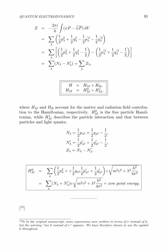
QUANTUM ELECTRODYNAMICS 91

Z = −2πi

h

∫(ψP − ψP ) dV

=∑

λ

(12p2

λ +12q2λ − 1

2p′2λ − 1

2q′2λ

)

=∑

λ

[(12p2

λ +12q2λ − 1

2

)−(

12p′2λ +

12q′2λ − 1

2

)]

=∑

λ

(Nλ − N ′λ) =

∑

λ

Zλ.

H = HM + HR,HM = H0

M + H1M ,

where HM and HR account for the matter and radiation field contribu-tion to the Hamiltonian, respectively. H0

M is the free particle Hamil-tonian, while H1

M describes the particle interaction and that betweenparticles and light quanta.

Nλ =12pλ2 +

12qλ2 − 1

2,

N ′λ =

12p′λ2 +

12q′λ2 −

12,

Zλ = Nλ − N ′λ.

H0M =

∑

λ

(12p2

λ + +12qλ2

12p′λ2 +

12q′λ2

)c

√

m2c2 + λ2h2

4π2

=∑

λ

(Nλ + N ′λ)c

√

m2c2 + λ2h2

4π2+ zero point energy.

——————–

[12]

12@ In the original manuscript, some expressions were written in terms of ν instead of k,but the warning “use k instead of ν” appears. We have therefore chosen to use the symbolk throughout.

92 E. MAJORANA: RESEARCH NOTES ON THEORETICAL PHYSICS

C =∑

k

AkQkfk +∑

λ

BλPλfλ,

−E =∑

k

CkPkfk −∑

λ

DλQλfλ

(∇×fλ = 0).∫

E2dV =∑

k

C2kP 2

k +∑

λ

D2λQ2

λ.

Hx =∂Cz

∂y− ∂Cy

∂z,

H2x =

(∂Cz

∂y

)2

+(

∂CH

∂r

)2

− 2∂Cx

∂y

∂Cy

∂x,

H2 =∑

x

|∇ Cx|2 −∑

xy

∂Cx

∂y

∂Cy

∂x=∑

k

A2kN

2Q2k.

∫H2dV = . . . .

PkQk − QkPk = 1/i,PλQλ − QλPλ = 1/i.

C2k

8π=

12

hck

2π,

A2k

8π=

12

hck

2π,

Dλ2

8π=

12;

Ck =√

2hck,

Ak =

√2hc

k,

Dλ =√

4π = 2√

π,

Bλ =hc√π

.

QUANTUM ELECTRODYNAMICS 93

Nk =12(P 2

k + Q2k) −

12.

C =∑

k

√2hc

kQkf

′k +

∑

λ

hc√π

Pλfλ,

−E =∑

k

√2hckPkf

′k −

∑

λ

√4πQλfλ.

νk = ck

2π.

HR =12

∑

k

hck

2π(Q2

k + P 2k ) +

12

∑

λ

Q2λ

=∑

k

12(P 2

k + Q2k) hνk +

12

∑

λ

Q2λ

=∑

k

Nhνk +∑

λ

12Q2

λ + rest energy.

——————–

[13]∇ uλ = ∇ λϕλ = λfλ,

∇ ψ =1√2

∑

λ

√mc

√m2c2 + λ2h2/4π2

[qλ + q′λ + i(pλ − p′λ)

]λfλ,

ψ∇ ψ − ψ∇ ψ = −imc∑

λλ′

14√

(m2c2 + λ2h2/4π2) (m2c2 + λ′h2/4π2)

×[(pλ − p′λ)(qλ′ + q′λ′)− (pλ′ − p′λ′)(qλ + q′λ)

]λ′uλfλ′ .

∇ ·ϕλfλ′ = fλ · fλ′ − λ′2ϕλϕλ′ .

13@ In the original manuscript, the expression ∇uλ = ∇λuλ = λfλ was written down,which is evidently incorrect.

94 E. MAJORANA: RESEARCH NOTES ON THEORETICAL PHYSICS

ψ =1√2

∑

λ

√mc

√m2c2 + h2λ2/4π2

[qλ + q′λ + i(pλ − p′λ)

]uλ,

P =h

4π√

2

∑

λ

√√m2c2 + h2λ2/4π2

mc

[pλ + p′λ + i(qλ − q′λ)

]uλ.

[14]

aλ =1√2(qλ + ipλ), bλ =

1√2(q′λ + ip′λ),

aλ =1√2(qλ − ipλ), bλ =

1√2(q′λ − ip′λ).

[aλ, aμ] − [bλ, bμ] − [aλ, bμ] − [bλ, aμ] = 2δλμ,

−[aλ, aμ] + [bλ, bμ] + [aλ, bμ] − [bλ, aμ] = 2δλμ.

[x, y] = xy ∓ yx,

where the upper/lower sign refers to Einstein/Fermi particles.

[aλ, aμ] + [bλ, bμ] + [aλ, bμ] + [bλ, aμ] = 0,[aλ, aμ] + [bλ, bμ] + [aλ, bμ] + [bλ, aμ] = 0,[aλ, aμ] + [bλ, bμ] + [aλ, bμ] + [bλ, aμ] = 0,[aλ, aμ] + [bλ, bμ] − [aλ, bμ] − [bλ, aμ] = 0,[aλ, aμ] + [bλ, bμ] − [aλ, bμ] − [bλ, aμ] = 0,[aλ, aμ] + [bλ, bμ] − [aλ, bμ] − [bλ, aμ] = 0,[aλ, aμ] − [bλ, bμ] + [bλ, aμ] − [aλ, bμ] = 0,[aλ, aμ] − [bλ, bμ] + [bλ, aμ] − [aλ, bμ] = 0.

2.8. CONTINUATION

ψ =∑

λ

√mc

√m2c2 + h2λ2/4π2

mc (aλ + bλ) uλ,

P =hi

4π

∑

λ

√√m2c2 + h2λ2/4π2

mc(aλ − bλ) uλ,

14@ In the original manuscript the simple formulas (a − ib)(a + ib) = a2 + b2 + i(ab − ba)and (a + ib)(a − ib) = a2 + b2 − i(ab − ba) are noted on the side.

QUANTUM ELECTRODYNAMICS 95

ψ =∑

λ

√mc

√m2c2 + h2λ2/4π2

(aλ + bλ) uλ,

P = − hi

4π

∑

λ

√√m2c2 + h2λ2/4π2

mc(aλ − bλ) uλ.

From the commutation relations reported at the end of the previous Sec-tion, we deduce that:

[aλ, aμ] +[bλ, bμ

]= 0,

[aλ, bμ

]+[bλ, aμ

]= 0,

[aλ, aμ] +[bλ, bμ

]= 0,

[aλ, bμ] +[bλ, aμ

]= 0,

[aλ, aμ] + [bλ, bμ] = 0,

[aλ, bμ] + [bλ, aμ] = 0,

[aλ, aμ] +[bλ, bμ

]= 0,

[bλ, bμ] + [aλ, bμ] = 0;

[aλ, aμ] −[bλ, bμ

]= 2δλμ,

[aλ, aμ] −[bλ, bμ

]= −2δλμ.

0 = [a + ib, a + ib] = [a, a] − [b, b] + i[a, b] + i[b, a],0 = [a − ib, a − ib] = [a, a] − [b, b] − i[a, b] − i[b, a],0 = [a + ib, a − ib] = [a, a] + [b, b] − i[a, b] + i[b, a],0 = [a − ib, a + ib] = [a, a] + [b, b] + i[a, b] − i[b, a];

[a, a] = [b, b] = [a, b] = [b, a] = 0.

2.9. QUANTIZED RADIATION FIELD

The author again considered the quantization of the electromagnetic field,but using now another expansion in a basis different from that adoptedin Sects. 2.4, 2.5. In the original manuscript, the present Section andthe following four Sections are placed in the Quaderno 17 just after whathas been here reported in Sect. 7.1.

E = −1c

∂C

∂t,

1c2

∂2C2

∂t2= ∇2 C = −1

c

∂E

∂t.

96 E. MAJORANA: RESEARCH NOTES ON THEORETICAL PHYSICS

Cx, Cy, Cz;

− Ex

4πc, − Ey

4πc, − Ez

4πc.

γ1, γ2, γ3 = 0,±1,±2, . . . ;

γ =c

k

√γ2

1 + γ22 + γ2

3 ;

px =h

kγ1, py =

h

kγ2, pz =

h

kγ3.

|ks| = 1, ks = k−s.

f s = ks e2πi(γsi x/k+γs

2y/k+γs3z/k) 1√

k3.

[15]

C =∑

asf s,

E =∑

bsf s.

as = a−s,

bs = b−s.

asas′ − as′as = 0,

bsbs′ − bs′bs = 0,

asbs′ − bs′as =2hc

iδs,s′ .

15@ In the original manuscript, the normalization factor 1/√

k3 is incorrectly treated as adenominator instead of a numerator.

QUANTUM ELECTRODYNAMICS 97

C = −cE =∑

−c bsf s; E = −c∇2 C =∑ 4π2ν2

s

casf s.

as = −c bs,

bs =4π2ν2

s

cas.

ddt

(as +

c

2πνsibs

)= −c bs − 2πνsi as = −2πνsi

(as +

c

2πνsibs

),

ddt

(as −

c

2πνsibs

)= −c bs + 2πνsi as = 2πνsi

(as −

c

2πνsibs

).

As = as +c

2πνsibs,

Bs = as −c

2πνsibs;

As = −2πνsi As,

Bs = 2πνsi Bs;

As = B−s,

Bs = A−s.

AsBs − BsAs = 0,

AsBs − BsAs = 0,

AsBs − BsAs = 0,

AsAs − AsAs =2hc2

πνs,

BsBs − BsBs = −2hc2

πνs.

98 E. MAJORANA: RESEARCH NOTES ON THEORETICAL PHYSICS

AsAt − AtAs = 0,

BsBt − BtBs = 0,

AsAt − AtAs = 0,

BsBt − BtBs = 0,

AsBt − BtAs = 0,

AsBt − BtAs = 0,

AsAt − AtAs =2hc2

πνsδst,

BsBt − BtBs = −2hc2

πνsδst.

Zs =1c

√πνs

2hAs.

ZsZt − ZtZs = 0,

ZsZt − ZtZs = 0,

ZsZt − ZtZs = δst.

ZsZs = ns.

< ns|Zs|ns+1 >=√

ns + 1,

< ns|Zs|ns−1 >=√

ns.

[16]

As = c

√2h

πνsZs,

16@ In the original manuscript, the unidentified Ref. 5.45 is here alluded to.

QUANTUM ELECTRODYNAMICS 99

as =As + A−s

2= c

√2h

πνs

Zs + Z−s

2,

bs =2πνsi

c

As − As

2= i

√2hπνs (Zs − Z−s).

Ws =18π

∑(bsbs +

4π2ν2s

c2asas

)

=18π

∑2hπνs

[(Zs − Z−s)(Zs − Z−s) + (Zs + Z−s)(Zs + Z−s)

]

=14

∑hνs{2ZsZs + 2Z−sZ−s}

=∑

hνsZsZs + Z−sZ−s

2=∑(

ns +12

)hνs.

f s =1

k3/2e2πi(γs

1x/k+γs2y/k+γs

3z/k)ks,

f−s =1

k3/2e−2πi(γs

1x/k+γs2y/k+γs

3z/k)ks = f s.

f s =1

k3/2e2πiγs·r/kks,

with r = (x, y, z).

C =∑

s

c

2

√2h

πνs(Zsf s + Zsf s),

E =∑

s

i√

2hπνs (Zsf s − Zsf s).

100 E. MAJORANA: RESEARCH NOTES ON THEORETICAL PHYSICS

E2(r) = −2hπ

k3

∑

s,t

√νsνt ks · kt

{ZsZt e2πi(γs+γt)·r/k

+ZsZt e−2πi(γs+γt)·r/k − ZsZt e2πi(γs−γt)·r/k

−ZsZt e2πi(−γs+γt)·r/k}

.

[17]

H2(r) = −2hπ

k3

∑

s,t

√νsνt k′

s · k′t

{ZsZt e2πi(γs+γt)·r/k

+ZsZt e−2πi(γs+γt)·r/k − ZsZt e2πi(γs−γt)·r/k

−ZsZt e2πi(−γs+γt)·r/k}

.

2.10. WAVE EQUATION OF LIGHT QUANTA

Quantized fields of the electromagnetic interaction were again consideredin these pages, with an emphasis (the name of this Section is the originalone) on the definition of a wavefunction ψ for the photon. Matrix ele-ments of the annihilation and creation operators Z, Z were reported inthe subsequent Section, along with quantum expressions for the photonenergy and angular momentum.[18]

C =∑

asf s, E =∑

bsf s;

as = c

√2h

πνs

Zs + Z−s

2, bs = i

√2hπνs (Zs − Z−s).

f s =1

k3/2e2πiγs·r/hks,

f s = f−s.

17C ∼ (e2πiγr/k, 0, 0), H ∼ (0, 2πi(γ/k) e2πγr/k, 0) .18@ The original manuscript alludes here to the unidentified Ref. 11.20.

QUANTUM ELECTRODYNAMICS 101

γs = (γs1, γ

s2, γ

s3),

γ1, γ2, γ3 = 0,±1,±2,±3, . . . ;

νs =c

kγs, hνs =

hc

kγs.

ψ =∑

Zsf s.

C =∑

s

c

√2h

πνs

Zs + Z−s

2f s =

∑

s

c

√2h

πνs

Zsf s + Zsf s

2,

E =∑

s

i√

2hπνs (Zs − Z−s)f s =∑

s

i√

2hπνs (Zsf s − Zsf s).

2.11. CONTINUATION

∇ ·C = 0.

1c

∂E

∂t= ∇×∇×C = −∇2 C,

1c

∂H

∂t− ∇×E =

1c

∂

∂t∇×C.

C =∑

c

√h

2πνs(Zsf s + Zsf s),

∂C

∂t=

∑c

√h

2πνs(Zsf s + ˙Zsf s),

∇2 C =∑ 2πνs

c

√2hπνs (Zsf s + Zsf s);

E =∑

i√

2hπνs (Zsf s − Zsf s),

∂E

∂t=

∑i√

2hπνs (Zsf s −˙Zsf s).

102 E. MAJORANA: RESEARCH NOTES ON THEORETICAL PHYSICS

i√

2hπνs (Zs − ˙Z−s) − 2πνs

√2hπνs (Zs + Z−s) = 0,

√h

2πνs(Zs + ˙Z−s) + i

√2hπνs(Zs − Z−s) = 0.

Zs − ˙Z−s = −2πiνs (Zs + Z−s),

Zs + ˙Z−s = −2πiνs (Zs − Z−s).

Zs = −2πiνsZs,˙Zs = 2πiνsZs,

˙Z−s = 2πiνsZ−s.

∫E2

8πdτ =

∑ hνs

4(Zs − Z−s)(Zs − Z−s)

=∑ hνs

4(ZsZs + Z−sZ−s − ZsZ−s − Z−sZs)

=∑ hνs

2

(ZsZs + ZsZs

2− ZsZ−s + ZsZ−s

2

)

.

∫H2

8πdτ =

∑ hνs

4(Zs + Z−s)(Zs + Z−s)

=∑ hνs

4(ZsZs + Z−sZ−s + ZsZ−s + Z−sZs)

=∑ hνs

2

(ZsZs + ZsZs

2+

ZsZ−s + ZsZ−s

2

)

.

∫E2 + H2

8πdτ =

∑hνs

ZsZs + ZsZs

2.

eiLx (0, 0, 1) = f s,

iLeiLx(0,−1, 0) = ∇×f s

f−s × ∇×f s = iL(1, 0, 0).

QUANTUM ELECTRODYNAMICS 103

Let us denote with rs a unitary vector along the propagation direction:

∫E × H

4πcdτ =

∑−hνs

2c(Zs − Z−s)(Zs + Z−s)rs

=∑ hνs

2crs (ZsZs − Z−sZ−s − Z−sZs − ZsZ−s)

=∑ hνs

crs

ZsZs + ZsZ−s

2.

ZsZs − ZsZs = 1.

ZsZs = X.

ZsX − XZs = (Zs, X) = Zs, Zik(Xk − Xi) = 1,

ZsX − XZs = (Zs, X) = −Zs, Zik(Xk − Xi) = −1.

< X|Z|X + 1 > = f(X),< X + 1|Z|X > = f(X).

< X|ZZ|X > = < X|Z|X − 1 >< X − 1|Z|X >= |f(X − 1)|2,< X|ZZ|X > = < X|Z|X + 1 >< X + 1|Z|X >= |f(X)|2;

|f(X)|2 = X + 1,

|f(X0)|2 = 1, X0 = 0.

|f(X)|2 = |f(X − 1)|2 + 1,

|f(X0)|2 = 1.

< X0|ZZ|X0 > = 0,

< X0|ZZ|X0 > = |f(0)|2.

ZsZs = ns, (ns = 0, 1, 2 . . .)

< ns|Zs|ns + 1 > =√

ns + 1,

< ns + 1|Zs|ns > =√

ns.

104 E. MAJORANA: RESEARCH NOTES ON THEORETICAL PHYSICS

f s = f−s.

∫E2 + H2

8πdτ =

∑hνs

(ns +

12

),

∫E × H

4πcdτ =

∑ hνs

crs

(ns +

12

).

2.12. FREE ELECTRON SCATTERING

The interaction between electrons and electromagnetic radiation was herestudied in detail, and expressions for the matrix elements of the inter-action energy (as well as for the transition probability) were explicitlyobtained. Some care was also devoted to the kinematics of the processhere considered. The material reported in this Section starts with thatpresent in Quaderno 17 on the page following 151bis, but the completestudy of the subject starts at page 133 of the same Quaderno.

[W

c+ ρ1 σ ·

(p +

e

cC)

+ ρ3 mc

]ψ = 0.

Using Dirac coordinates:

ψr = ur1√k3

e2πi(Γ r1x/k+Γ r

2y/k+Γ r3z/k).

ur = (ur1, ur

2, ur3, ur

r), uuur = 1, Γ =√

Γ r1 + Γ r

2 + Γ r3.

Er = ±c

√

m2c2 +h2

k2Γ 2 .

H = H0 + I,

H0 = −c ρ1 σ · p − ρ3 mc2 +∑

s

nshνs,

I = −c ρ1 σ · e

cC = −e ρ1 σ · C.

QUANTUM ELECTRODYNAMICS 105

< . . . |H0| . . . > = Er +∑

nshνs,

< r;ns . . . |I|r′;ns + 1 . . . > = −√

ns + 1ec

2

√2h

πνs

×∫

ψr ρ1σ · f s ψr′ dτ,

< r;ns . . . |I|r′;ns − 1 . . . > = −√ns

ec

2

√2h

πνs

×∫

ψr ρ1 σ · f−s ψr′ dτ.

ψr = ur1

k3/2e2πiΓ r·r/k,

ψr′ = ur′1

k3/2e2πiΓ r′ ·r/k,

f s = ks1

k3/2e2πiγs·r/k,

f−s = f s

1k3/2

e−2πiγs·r/k.

ks = k−s.

∫ψr ρ1σ · f s ψr′ dτ = k−7/2 ur ρ1 σ · ks ur′

×∫

e2πi(Γ r′+γs−Γ r

)·r/kdτ

=ur ρ1 σ · ks ur′

k7/2δΓ r

, Γ r′+γs

,

∫ψr ρ1σ · f−s ψr′ dτ =

ur ρ1 σ · ks ur′

k7/2δΓ r

, Γ r′−γs.

< r;ns . . . |I|r′;ns + 1 . . . > = − ec

2k3/2

√ns + 1

√2h

πνs

× ur ρ1 σ · ks ur′ δΓ r,Γ r′

+γs,

< r;ns . . . |I|r′;ns − 1 . . . > = − ec

2k3/2

√ns

√2h

πνs

× ur ρ1 σ · ks ur′ δΓ r,Γ r′−γs

.

106 E. MAJORANA: RESEARCH NOTES ON THEORETICAL PHYSICS

For t = 0: a1 = 1, a2, . . . = 0.For t → 0:

ai = −2πi

he2πi(Ei−E1)t/h Hi1;

ai = − 1Ei − E1

(e2πi(Ei−E1)t/h − 1

)Hi1.

H12 = 0.

a2 = −2πi

h

∑

i

−1Ei − E1

e2πi(E2−Ei)t/h(e2πi(Ei−E1)t/h − 1

)H2iHi1

=2πi

h

∑

i

1Ei − E1

(e2πi(E2−E1)t/h − e2πi(E2−Ei)t/h

)H2iHi1;

a2 =∑

i

[1

(Ei − E1)(E2 − E1)

(e2πi(E2−E1)t/h − 1

)

− 1(E2 − Ei)(Ei − E1)

e2πi(E2−Ei)t

]H2iHi1.

electron radiation

2 b nt = 1

i, i′ r, r′↗↘

↘↗ nt = 1, ns = 1

1 a ns = 1

Γ a + γs = Γ b + γt = Γ r = Γ r′ + γs + γt

s, t label the incident and the scattered quanta, respectively.

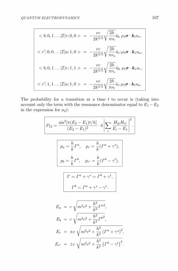
QUANTUM ELECTRODYNAMICS 107

< b; 0, 1 . . . |I|r; 0, 0 > = − ec

2k3/2

√2h

πνtub ρ1σ · ktur,

< r′; 0, 0 . . . |I|a; 1, 0 > = − ec

2k3/2

√2h

πνsur′ρ1σ · ksua,

< b; 0, 1 . . . |I|r; 1, 1 > = − ec

2k3/2

√2h

πνsub ρ1σ · ksur,

< r′; 1, 1 . . . |I|a; 1, 0 > = − ec

2k3/2

√2h

πνtur′ρ1σ · ktua.

The probability for a transition at a time t to occur is (taking intoaccount only the term with the resonance denominator equal to E1−E2

in the expression for a2):

P12 =sin2[π(E2 − E1)t/h]

(E2 − E1)2· 4

∣∣∣∣∣

∑

i

H2iHi1

Ei − E1

∣∣∣∣∣

2

.

pa =h

kΓ a, pr =

h

k(Γ a + γs),

pb =h

kΓ b, pr′ =

h

k(Γ b − γt).

Γ = Γ a + γs = Γ b + γt,

Γ b = Γ a + γs − γt.

Ea = c

√

m2c2 +h2

k2Γ a2,

Eb = c

√

m2c2 +h2

k2Γ b2,

Er = ±c

√

m2c2 +h2

k2(Γ a + γs)2,

Er′ = ±c

√

m2c2 +h2

k2

(Γ b − γt

)2.

108 E. MAJORANA: RESEARCH NOTES ON THEORETICAL PHYSICS

E1 = c

√

m2c2 +h2

k2Γ a2 + hνs,

E2 = c

√

m2c2 +h2

k2(Γ a + γs − γt)2 + hνt,

Ei = ±c

√

m2c2 +h2

k2(Γ a + γs)2,

Ei′ = ±c

√

m2c2 +h2

k2(Γ a − γt)2 + hνs + hνt.

Let us denote by u the spin function for a plane wave with momentumpx, py, pz and by u0 that for a wave of zero momentum.

up =[f1 ∓ f2

α · pp

]u0,

where the upper/lower sign refers to positive/negative energy waves.

f1 =

√1 +

√1 + p2/m2c2

2√

1 + p2/m2c2, f2 =

√−1 +

√1 + p2/m2c2

2√

1 + p2/m2c2;

|f21 | + |f2

2 | = 1.

α = ρ1 σ.

ub =[f b1 − f b

2

α · pb

pb

]u0

b , ur

[f r1 ∓ f r

2

α · pr

pr

]u0

r ,

ua =[fa1 − f b

2

α · pa

pa

]u0

a, ur′

[f r′1 ∓ f r′

2

α · pr′

pr′

]u0

r′ .

We consider positive waves ua, ub.

QUANTUM ELECTRODYNAMICS 109

[19]

1) Positive ur:

ub α · kt ur ur α · ks ua

= u0b

(f b1 − f b

2

α · pb

pb

)α · kt

(f r1 − f r

2

α · pr

pr

)u0

r

× u0r

(f r1 − f r

2

α · pr

pr

)α · ks

(fa1 − fa

2

α · pa

pa

)u0

a

= u0b

[f b1α · ktf

r2

α · pr

pr+ f b

2

α · pb

pbα · ktf

r1

]u0

r

× u0r

[f r1α · ksf

a2

α · pa

pa+ f r

2

α · pr

prα · ksf

a1

]u0

a.

2) Negative ur:

ub α · kt ur ur α · ks ua

= u0b

[f b1f r

1α · kt − f b2f r

2

α · pb

pbα · kt

α · pr

pr

]u0

r

× u0r

[f r1fa

1 α · ks − f r2fa

2

α · pr

prα · ks

α · pa

pa

]u0

r .

3) Positive ur′ :

ub α · ks ur′ ur′α · kt ua = . . .

[which is obtained from 1) with the replacements r → r′, ks → kt,kt → ks].

4) Negative ur′ :

ub α · ks ur′ ur′ α · kt ua = . . .

[which is obtained from 1) with the replacements r → r′, ks → kt,kt → ks].

19@ The original manuscript alludes here to the unidentified Ref. 10.40.

110 E. MAJORANA: RESEARCH NOTES ON THEORETICAL PHYSICS

1)∑

positive ur

ub α · kt ur urα · ks ua

= u0b

[f b1f r

2α · ktα · pr

pr+ f r

1f b2

α · pb

pbα · kt

]

×[f r1fa

2 α · ksα · pa

pa+ f r

2fa1

α · pr

prα · ks

]u0

a

= u0b

[f b1f r

2σ · ktσ · pr

pr+ f b

2f r1

σ · pb

pbσ · kt

]

×[f r1fa

2 σ · ksσ · pa

pa+ f r

2fa1

σ · pr

prσ · ks

]u0

a.

(σ · kt)(σ · pr) = kt · pr + iσ · kt × pr,

(σ · kt)(σ · pr)(σ · ks)(σ · pr)= (kt · pr)(ks · pa) + i(kt · pr)(σ · ks × pa)

+ i(ks · pa)(σ · kp × pr) − (σ · kt × pr)(σ · ks × pa)

=(kt · pr)(ks · pa) + i(kt · pr)(σ · ks × pa)+i(ks · pa)(σ · kt × pr) − (kt × pr)(ks × pa)−i[σ, (kt × pr) × (ks × pa)].

For ua = u0a, pa = 0: fa

1 = 1, fa2 = 0.

——————–

1)∑

positive ur

ub α · kt ur urα · ks ua

= u0b

[f b1f r

2σ · ktσ · pr

pr+ f b

2f r1

σ · pb

pbσ · kt

]f r2

σ · pr

prσ · ks u0

a.

For ks · pr = 0:

(σ · kt)(σ · pr)(σ · pr)(σ · ks) = p2r(σ · kt)(σ · ks)

= p2r(kt · ks) + ip2

r(σ · kt × ks),

(σ · pb)(σ · kt)(σ · pr)(σ · ks) = (pb · kt + iσ · pb × kt) iσ · pr × ks

= −(pb × kt) · (pr × ks) + i(pb · kt)(σ · pr × ks)− iσ · (pb × kt) × (pr × ks).

QUANTUM ELECTRODYNAMICS 111

2)∑

negative ur

ub α · kt ur ur α · ks ua

= u0b

[f b1f b

1σ · kt − f b2f b

2

σ · pb

pbσ · kt

σ · pr

pr

]f r1σ · ksu

0a.

3)∑

positive ur′

ub α · ks ur′ ur′ α · kt ua

= u0b

[f b1f r′

2 σ · ksσ · pr′

pr′− f b

2f r′1

σ · pb

pbσ · ks

]f r′2

σ · pr′

pr′σ · kt u0

a.

4)∑

negative ur′

ub α · ks ur′ ur′ α · kt ua

= u0b

[f b1f r′

1 σ · ks − f b2f r′

2

σ · pb

pbσ · ks

σ · pr

pr

]f r′1 σ · kt u0

a.

——————–

Let us denote with η the average value with respect to u0b and u0

a:

|u0bAu0

a|2 = u0bAu0

aAu0b =

12u0

bAAu0a =

14[(AA)11 + (AA)22].

A = A0 + iσ · B,

AA = [A0 + iσ · B][A0 − iσ · B]= A0A0 + iA0σ · B − iA0σ · B + B · B + iσ · B × B.

AA = A0A0 + B · B, |ub0Aua

0|2 =12A0A0 +

12B · B.

γs = (γs, 0, 0), ks = (0, 0, 1), γt = (γt sin ϑ cos ϕ, γt sin ϑ sin ϕ, γt cos ϑ).Near the resonance we have:

νt =νs

1 +hνs

mc2(1 − sin ϑ cos ϕ)

.

pr =hνs

c(1, 0, 0), pr′ = −hνt

c(sin ϑ cos ϕ, sin ϑϕ, cos ϑ),

112 E. MAJORANA: RESEARCH NOTES ON THEORETICAL PHYSICS

pb =hνt

c

((1 +

hνs

mc2

)(1 − sin ϑ cos ϕ), − sin ϑ sin ϕ, − cos ϑ

).

E1 = mc2 + hνs,

E′1 = ±

√m2c4 + h2ν2

t + hνs + hνt,

Ei = ±√

m2c4 + h2ν2s ,

Er ∼ E1.

2.13. BOUND ELECTRON SCATTERING

Let us consider f bound electrons; the unperturbed energy of the systeminteracting with an electromagnetic field is En+

∑s nshνs. Denoting with

ψa(q1, . . . , qf ) the electron wavefunction corresponding to energy Ea, theinteraction with the electromagnetic field is described by:

< a;ns . . . |I|b;ns + 1 . . . > = −e c

√h(ns + 1)

2πνs

×∫

ψa

f∑

i=1

αi · f s(q1) ψf dτ,

< a;ns . . . |I|b;ns − 1 . . . > = −e c

√hns

2πνs

×∫

ψa

f∑

i=1

αi,f s(q1) ψf dτ.

αi = ρi1 σi.

In first approximation, λ � |qi|;

fs(qi) ∼ fs(0) =ks

k3/2.

For coherent scattering , by labelling with S, t the incident and scatteredquantum, respectively, with wave-vectors ks, kt, we have:

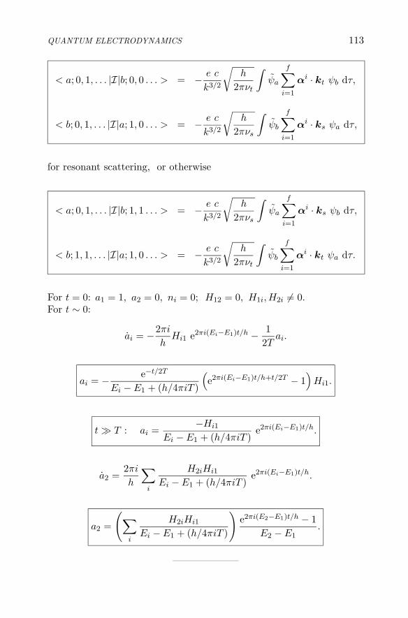
QUANTUM ELECTRODYNAMICS 113

< a; 0, 1, . . . |I|b; 0, 0 . . . > = − e c

k3/2

√h

2πνt

∫ψa

f∑

i=1

αi · kt ψb dτ,

< b; 0, 1, . . . |I|a; 1, 0 . . . > = − e c

k3/2

√h

2πνs

∫ψb

f∑

i=1

αi · ks ψa dτ,

for resonant scattering, or otherwise

< a; 0, 1, . . . |I|b; 1, 1 . . . > = − e c

k3/2

√h

2πνs

∫ψa

f∑

i=1

αi · ks ψb dτ,

< b; 1, 1, . . . |I|a; 1, 0 . . . > = − e c

k3/2

√h

2πνt

∫ψb

f∑

i=1

αi · kt ψa dτ.

For t = 0: a1 = 1, a2 = 0, ni = 0; H12 = 0, H1i,H2i �= 0.For t ∼ 0:

ai = −2πi

hHi1 e2πi(Ei−E1)t/h − 1

2Tai.

ai = − e−t/2T

Ei − E1 + (h/4πiT )

(e2πi(Ei−E1)t/h+t/2T − 1

)Hi1.

t � T : ai =−Hi1

Ei − E1 + (h/4πiT )e2πi(Ei−E1)t/h.

a2 =2πi

h

∑

i

H2iHi1

Ei − E1 + (h/4πiT )e2πi(Ei−E1)t/h.

a2 =

(∑

i

H2iHi1

Ei − E1 + (h/4πiT )

)e2πi(E2−E1)t/h − 1

E2 − E1.

——————–

114 E. MAJORANA: RESEARCH NOTES ON THEORETICAL PHYSICS

When a variable magnetic field H = H(t) is included in the interaction,we have to consider also the diagonal magnetic moments μi. For Hx =Hy = 0,Hz = H(t):

a1 =2πi

hH(t) μ1 a1,

a1 = e(2πi)/h μ1

∫Hdt

.

ai = −2πi

hHi1 e2πi(Ei−E1)t/h e

(2πi)/h μ1

∫Hdt

− 12T

ai +2πi

hH μi ai.

ai = e−t/2T e(2πi)/h μi

R

Hdt

(−2πi

hHi1

)

×

⎡

⎢⎣∫

e2πi(Ei − E1)t/h + t/2T + (2πi)/h (μ1 − μi)

∫Hdt

dt + C

⎤

⎥⎦ .

a2 = −2πi

h

∑

i

H2i e2πi(E2−E1)t/hai +2πi

hHμ2a2.

a2 =(−2πi

h

)e(2πi/h) μ2

∫Hdt

×

⎡

⎢⎣∑

H2i

∫ t

0e2πi(E2 − Ei)t/h − (2πi/h) μ2

∫Hdt

ai dt

⎤

⎥⎦ .

H = H0 cos 2πνt,∫

Hdt =H0

2πνsin 2πνt,

2π

h(μ1 − μi)

∫Hdt =

H0(μ1 − μ − i)hν

sin 2πνt,

QUANTUM ELECTRODYNAMICS 115

e(2πi/h)(μ1 − μi)

∫Hdt

= ei[H0(μ1 − μi)/hν] sin 2πνt

= eiAi sin 2πνt,

Ai =H0(μ1 − μi)

hν.

[20]

eiAi sin 2πνt = ci0 + ci

i e2πνit + ci−1 e−2πνit + ci

2e4πνit + ci

−2 e−4πνit + . . . .

ω = 2πνt:

eiAi sin ω = ci0 + ci

1 eiω + ci−1 e−iω + ci

2 e2iω + ci−2 e−2iω + . . . .

ci0 =

12π

∫ 2π

0eiAi sin ω dω.

ζ = eiω, sin ω =ζ − ζ−1

2i, dζ = iζdω, dω = −i

dζ

ζ;

eiAi sin ωdω =1iζ

eAi(ζ−ζ−1)/2dζ.

ci0 =

12πi

∮1ζeAi(ζ−ζ−1)/2dζ.

eAi(ζ−ζ−1)/2 = 1+Aiζ − ζ−1

2+

A2i

2!

(ζ − ζ−1

2

)2

+A3

i

3!

(ζ − ζ−1

2

)3

+ . . . .

(ζ − ζ−1

)n =n∑

r=0

ζn−2r

(nr

)(−1)r,

20@ The original manuscript alludes here to the unidentified Ref. 11.05.

116 E. MAJORANA: RESEARCH NOTES ON THEORETICAL PHYSICS

(ζ − ζ−1

)2n =2n∑

r=0

(−1)rζ2n−2r

(2nr

)

=n∑

s=−n

(−1)n

(2n

n + s

)ζ−2s(−1)s(−1)n

(2nn

)

=(2n)!n!2

(−1)n.

ci0 = 1 − A2

i

1 · 22+

A4i

2!2 · 24− . . . = I0(Ai).

2.14. RETARDED FIELDS

The possibility is considered, in the following pages, of introducing anintrinsic constant time delay τ (or an intrinsic space constant ε = cτ)in the expressions for the electromagnetic retarded fields, generically de-noted with f(x, y, z, t).

f = f(x, y, z, t).

ϕ(x, y, z, t) = f(x, y, z, t − r

c

)= f(x, y, z, t).

ϕ′x(x, y, z, t) = f ′

x

(x, y, z, t − r

c

)− x

rcf ′

t

(x, y, z, t − r

c

)

= f ′x(x, y, z, t) − x

rcf ′

t(x, y, z, t),

ϕ′′x(x, y, z, t) = f

′′

x2

(x, y, z, t − r

c

)− 2x

rcf

′′xt

(x, y, z, t − r

c

)

+x2

r2c2f

′′tt

(x, y, z,−r

c

)− r2 − x2

r3cf ′

t

(x, y, z, t − r

c

)

= f ′′xx(x, y, z, t) − 2x

rcf

′′xt(x, y, z, t) +

x2

r2c2f

′′tt(x, y, z, t)

−r2 − x2

r3cf ′

t(x, y, z, t).

ϕ′t(x, y, z, t) = f ′

t

(x, y, z, t − r

c

)= f ′

t(x, y, z, t),

ϕ′′tt(x, y, z, t) = f

′′t

(x, y, z, t − r

c

)= f

′′tt(x, y, z, t).

QUANTUM ELECTRODYNAMICS 117

� = ∇2 − 1c2

∂2

∂t2:

�ϕ(x, y, z, t) = ∇2 f(x, y, z, t − r

c

)− 2

c

∂2

∂r∂t(x, y, z, t)

− 2rc

f ′t(x, y, z, t),

∂

∂rϕ(x, y, z, t) =

∑

x

x

rf ′

x

(x, y, z, t − r

c

)− 1

cf ′

t

(x, y, z, t − r

c

)

=∂

∂zf(x, y, z, t) − 1

cf ′

t(x, y, z, t),

∂2

∂r∂tϕ(x, y, z, t) =

∂2

∂r∂tf(x, y, z, t) − 1

cf

′′t (x, y, z, t).

�ϕ +2c

∂2

∂z∂tϕ = ∇2 f − 2

c2f

′′t − 2

rcf ′

t

= �f − 1c2

f′′t − 2

rcf ′

t.

�f = ∇2 ϕ +2rc

ϕ′ +2c

∂2

∂z∂tϕ.

——————–

ϕ(x, y, z, t) = f

(

x, y, z, t −√

r2 + ε2

c

)

= f(x, y, z, t).

f(x, y, z, t) = ϕ

(

x, y, z, t −√

r2 + ε2

c

)

,

f ′x(x, y, z, t) = ϕ′

x

(

x, y, z, t −√

r2 + ε2

c

)

+x

c√

r2 + ε2ϕ′

t

(

x, y, z, t +√

r2 + ε2

c2

)

,

118 E. MAJORANA: RESEARCH NOTES ON THEORETICAL PHYSICS

f′′xx(x, y, z, t) = ϕ

′′x

(

x, y, z, t +√

r2 + ε2

c

)

+2x

c√

r2 + ε2ϕ

′′xt

(

x, y, z, t +√

r2 + ε2

c2

)

+r2 + ε2 − x2

c(r2 + ε2)3/2ϕ′

t

(

x, y, z, t +√

r2 + ε2

c

)

+x2

c2(r2 + ε2)ϕ

′′tt

(

x, y, z, t +√

r2 + ε2

c

)

,

f′′tt(x, y, z, t) = ϕ

′′tt

(

x, y, z, t +√

r2 + ε2

c

)

.

�f′′tt(x, y, z, t) = ∇2 ϕ

(

x, y, z, t +√

r2 + ε2

c

)

− ε2

c2(r2 + ε2)ϕ

′′tt

(

x, y, t +√

r2 + ε2

c

)

+2r2 + 3ε2

c(√

r2 + ε2)3ϕ′

t

(

x, y, z, t +√

r2 + ε2

c

)

+2r

c√

r2 + ε2

∂2

∂r∂tϕ

(

x, y, z, t +√

r2 + ε2

c

)

.

�f = ∇2 ϕ − ε2

c2(r2 + ε2)ϕ +

2r2 + 3ε2

c(r2 + ε2)3/2ϕ +

2z

c√

r2 + ε2

∂2

∂r∂tϕ.

2.14.1 Time DelayWith the introduction of a time delay τ , which is a universal constant(classically τ = 0), by setting

ε = τc ,

QUANTUM ELECTRODYNAMICS 119

we get:

Φ =∫

1√r2 + ε2

S

(t −

√z2 + ε2

c, x, y, z

)dxdy dz,

and, for ε → 0:

Φ =∫

1rS(t − r

c, x, y, z

)dxdy dz

−ε2

{∫1

2r3S(t − r

c, x, y, z

)dxdy dz

+∫

12r2c

S(t − r

c, x, y, z

)dxdy dz

}+ . . . .

2.15. MAGNETIC CHARGES

A modification of the classical Maxwell equations was considered in thefollowing pages, in order to include also the effect of magnetic charges.

A(q) = − 14π

∫ ∇ · g(q′)r

dq′.

g0 = − 14π

∇∫ ∇ · g(q′)

rdq′,

g1 = g − g0.

g = (δ(q − q0); 0; 0),

∇ · g = δ′(x − x0) δ(y − y0) δ(z − z0).r = |q′ − q|:

∫δ′(x′ − x0) δ(y − y0) δ(z − z0)

rdq′

=∫

δ′(x′ − x0)√(y0 − y)2 + (z0 − z)2 + (x′ − x)2

dx′

=∫

δ(x′ − x0)x′ − x

[(y0 − y)2 + (z0 − z)2 + (x′ − x)2]3/2dx′

= − x − x0

[(x − x0)2 + (y − y0)2 + (z − z0)2]3/2

= −x − x0

R3.

120 E. MAJORANA: RESEARCH NOTES ON THEORETICAL PHYSICS

g01 =

3(x − x0)2 − R2

R5, g0

2 =3(x − x0)(y − y0)

R5,

g03 =

3(x − x0)(z − z0)R5

;

g11 = δ(q − q0) −

3(x − x0)2 − R2

R5, g1

2 = −3(x − x0)(y − y0)R5

,

g13 = −3(x − x0)(z − z0)

R5.

——————–

E =E′ + E′′

2, H =

H ′ + H ′′

2.

4πI∫

+1c

∂E′

∂t= ∇×H ′, 4πI +

1c

∂E′′

∂t= ∇×H ′′,

−4πI − 1c

∂H ′

∂t= ∇×E′, 4πI − 1

c

∂H ′′

∂t= ∇×E′′,

∇ ·E′ = 4πρ, ∇ ·E′′ = 4πρ,

∇ ·H ′ = 4πρ, ∇ ·H ′′ = −4πρ.

⎧⎪⎨

⎪⎩

4πI (1 − i) +1c

∂(E′ − iH ′)∂t

= i∇× (E′ − iH ′),

∇ · (E′ − iH ′) = 4πρ (1 − i),

⎧⎪⎨

⎪⎩

4πI (1 + i) +1c

∂(E′′ − iH ′′)∂t

= i∇× (E′′ − iH ′′),

∇ · (E′′ − iH ′′) = 4πρ (1 + i),

QUANTUM ELECTRODYNAMICS 121

⎧⎪⎨

⎪⎩

4πI (1 + i) +1c

∂(E′ + iH ′)∂t

= −i∇× (E′ + iH ′),

∇ · (E′ + iH ′) = 4πρ (1 + i),

⎧⎪⎨

⎪⎩

4πI (1 − i) +1c

∂(E′′ + iH ′′)∂t

= −i∇× (E′′ + iH ′′),

∇ · (E′′ + iH ′′) = 4πρ (1 − i),

For E′ = −H ′′, H ′ = E′′ we re-obtain the Maxwell equations:

E =E′ + H ′

2, H =

H ′ − E′

2.

[21]

Appendix:Potential experienced by an electric charge: a par-ticular case

For a charge-1 particle:

dV

dt= − 1

2(a2 + t)(a2 + t)(c2 + t)= − 1

2(a2 + t)√

c2 + t,

21@ The page ended with an attempt to generalize the above results to arbitrary linear com-binations of the E and H fields (with space-time dependent coefficients), in the case ofMaxwell equations without sources:

E′ = αE + βH, H′ = −βE + αH;

α = α(q, t), β = β(q, t);

1

c

∂E

∂t= ∇×H, −1

c

∂H

∂t= ∇×E,

∇ ·E = 0, ∇ ·H = 0;

∇ ·E′ = ∇α · E + ∇β · H,

∇ ·H′ = −∇β · E + ∇α · H.

122 E. MAJORANA: RESEARCH NOTES ON THEORETICAL PHYSICS

−1c

= V =∫ ∞

0

dt

2(a2 + t)√

(c2 + t)

=∫ ∞

c

dz

z2 + (a2 − c2)=

1√a2 − c2

(π

2− arctan

c√a2 − c2

)

=1√

a2 − c2arctan

√a2 − c2

c.

z =√

c2 + t,

z2 = c2 + t,

dt = 2z dz,

t = z2 − c2,

a2 + t = z2 + (a2 − c2).

c = a√

1 − β2, a2 − c2 = a2β2.

1c

= V =1aβ

arctanβ√

1 − r2=

1aβ

arcsin β.

c = aβ

arcsin β; V =

1c

=1a

arcsin β

β.

(∂Cx

∂z− ∂Cz

∂Cx

)2

+(

∂Cy

∂x− ∂Cx

∂y

)2

+(

∂Cz

∂y− ∂Cy

∂z

)2

= |∇ Cx|2 + |∇ Cy|2 + |∇ Cz|2 −∑

xy

∂Cx

∂y

∂Cy

∂x.

PART II

3

ATOMIC PHYSICS

3.1. GROUND STATE ENERGY OF ATWO-ELECTRON ATOM

Let us consider a nucleus of charge Z with two electrons. In electronicunits we have:

∇2 ψ + 2(E − V )ψ = 0,

V = −Z

r1− Z

r2+

1r3

.

In the same units, but denoting with W the energy in rydberg, we haveW = 2E and thus:

Wψ = V ψ − ∇2 ψ,

that is:

Wψ = −2Z

(1r1

+1r2

)ψ +

2r3

ψ − ∇2 ψ = Hψ.

3.1.1 Perturbation MethodIn first approximation, neglecting the interaction and up to a normal-ization constant, we have:

125

126 E. MAJORANA: RESEARCH NOTES ON THEORETICAL PHYSICS

ψ = e−Zr1 e−Zr2 ,

and:

H0ψ = W0ψ = −2Z2ψ,

where H0 is the unperturbed Hamiltonian:

H0 = −2Z

(1r1

+1r2

)− ∇2 .

In fact:

∇2 ψ =∂2ψ

∂r21

+∂2ψ

∂r22

+2r1

∂ψ

∂r1+

2r2

∂ψ

∂r2= 2Z2ψ − 2Z

(1r1

+1r2

)ψ.

In first approximation, assuming a normalized ψ, we have:

dW =∫

2r3

ψ2dτ,

and since, evidently,

W0 =∫

ψH0ψdτ,

more expressively we can write:

W = W0 + ΔW =∫

ψ

(H0 +

2r

)ψdτ =

∫ψHψdτ.

The correct value W appears, then, to be the mean value of the energyrelative to the function ψ that, in first approximation, coincides withthe energy eigenfunction. This will be useful in comparing the resultsobtained with the perturbation method with those of the variationalmethod.1

We thus have:

dW =

∫2r3

e−2Z(r1+r2)dτ∫

e−2Z(r1+r2)dτ

.

The integration with respect to the angular coordinates gives:

1@ In the original manuscript, the variational method is appropriately called the “minimummethod”.

ATOMIC PHYSICS 127

dW =2∫∫

r21r

22

1ρ

e−2Z(r1+r2)dr1 dr2

∫∫r21r

22 e−2Z(r1+r2)dr1dr2

,

where ρ is the greater value between r1 and r2. By restricting the doubleintegration field to the region r1 ≤ r2, the numerator and the denomi-nator will be divided by a factor two, so that:

dW =

∫ ∞

02r2 e−2Zr2dr2

∫ r2

0r21 e−2Zr1dr1

∫ ∞

0r22 e−2Zr2dr2

∫ r2

0r21 e−2Zr1dr1

.

Now we have:∫

r21 e−2Zr1dr1 = − r2

1

2Ze−2Zr1 +

1Z

∫r1e−2Zr1dr1

= − r21

2Ze−2Zr1 − r1

2Z2e−2Zr1 +

12Z2

∫e−2Zr1dr1

=(− r2

1

2Z− r1

2Z2− 1

4Z3

)e−2Zr1 ,

so that:∫ r2

0r21 e−2Zr1dr1 =

14Z3

−(

14Z3

+r2

2Z2+

r22

2Z

)e−2Zr2 .

We thus have:dW =

N

D,

N =∫ ∞

0

r2

2Z3e−2Zr2dr2 −

∫ ∞

0

r2

2Z3e−4Zr2dr2 −

∫ ∞

0

r22

Z2e−4Zr2

−∫ ∞

0

r22

Ze−4zr2dr2

=1

8Z5− 1

32Z5− 1

32Z5− 3

128Z5=

5128Z5

,

D =∫ ∞

0

r22

4Z3e−2Zr2dr2 −

∫ ∞

0

r22

4Z3e−4Zr2dr2 −

∫ ∞

0

r32

2Z2e−4Zr2dr2

−∫ ∞

0

r42

2Ze−4Zr2dr2

=1

16Z6− 1

128Z6− 3

256Z6− 3

256Z6=

132Z6

,

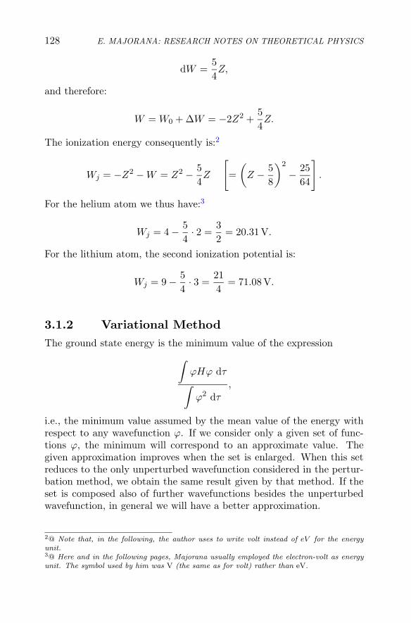
128 E. MAJORANA: RESEARCH NOTES ON THEORETICAL PHYSICS

dW =54Z,

and therefore:

W = W0 + ΔW = −2Z2 +54Z.

The ionization energy consequently is:2

Wj = −Z2 − W = Z2 − 54Z

[

=(

Z − 58

)2

− 2564

]

.

For the helium atom we thus have:3

Wj = 4 − 54· 2 =

32

= 20.31 V.

For the lithium atom, the second ionization potential is:

Wj = 9 − 54· 3 =

214

= 71.08 V.

3.1.2 Variational MethodThe ground state energy is the minimum value of the expression

∫ϕHϕ dτ

∫ϕ2 dτ

,

i.e., the minimum value assumed by the mean value of the energy withrespect to any wavefunction ϕ. If we consider only a given set of func-tions ϕ, the minimum will correspond to an approximate value. Thegiven approximation improves when the set is enlarged. When this setreduces to the only unperturbed wavefunction considered in the pertur-bation method, we obtain the same result given by that method. If theset is composed also of further wavefunctions besides the unperturbedwavefunction, in general we will have a better approximation.

2@ Note that, in the following, the author uses to write volt instead of eV for the energyunit.3@ Here and in the following pages, Majorana usually employed the electron-volt as energyunit. The symbol used by him was V (the same as for volt) rather than eV.

ATOMIC PHYSICS 129

3.1.2.1 First case. To this end, we consider the functions

ϕ = e−k(r1+r2)

with arbitrary k. We have:

Hϕ = −2k2ϕ + 2(k − Z)(

1r1

+1r2

)ϕ +

2r3

ϕ,

∫ϕHϕ dτ

∫ϕ2 dτ

= −2k2 + 4(k − r)

∫ ∞

0r1 e−2kr1dr1

∫ ∞

0r21 e−2kr1dr1

+54k

= −2k2 + 4(k − Z)k +54k,

that is:

Wmean = 2k2 − 4kZ +54k.

The minimum will be reached when:

4k − 4Z +54

= 0,

that is:

k = Z − 516

.

In this case we have:

W = 2(

Z − 516

)2

− 4Z

(Z − 5

16

)+

54

(Z − 5

16

),

that is:

W = −2Z2 +54Z − 25

128= −2

(Z − 5

16

)2

= −2k2.

The ionization energy will be

Wj = −Z2 − W = Z2 − 54Z +

25128

.

For the helium atom:

Wj =217128

= 22.95 V.

130 E. MAJORANA: RESEARCH NOTES ON THEORETICAL PHYSICS

3.1.2.2 Second case. Let ϕ be an arbitrary function; thewavefunction of the ground state can be approximated by an expressionof the form:

y = aϕ + bHϕ,

so that we have:

Wmean =

∫yHy dτ∫

y2 dτ

=

∫(aϕ + bHϕ)(aHϕ + bH2ϕ) dτ

∫(aϕ + bHϕ)2 dτ

=a2

∫ϕHϕ dτ + b2

∫Hϕ · H2ϕ dτ + ab

∫Hϕ · Hϕ dτ + ab

∫Hϕ · Hϕ dτ

a2

∫ϕ2 dτ + b2

∫Hϕ · Hϕ dτ + 2ab

∫ϕ · dτ

By noting that∫ (

Hϕ · Hϕ − ϕ H2ϕ)

dτ =∫

[(Hϕ)Hϕ − ϕH(Hϕ)] dτ = 0

or: ∫Hϕ · Hϕ dτ =

∫ϕ · H2ϕ dτ,

and, in general,∫

Hmϕ · Hnϕ dτ =∫

ϕHm+nϕ dτ,

we get:

Wmean =a2A + 2abB + b2C

a2 + 2abA + b2B,

where

A =

∫ϕ · Hϕ dτ∫

ϕ2 dτ

, B =

∫ϕ · H2ϕ dτ∫

ϕ2 dτ

, C =

∫ϕ · H3ϕ dτ∫

ϕ2 dτ

.

If we consider the generalized trial function

y = a0ϕ + a1Hϕ + a2H2ϕ + . . . + anHnϕ,

ATOMIC PHYSICS 131

we analogously get:

Wmedia =

n∑

i,k=0

aiak Ai+k+1

n∑

i,k=0

aiak Ai+k

,

where:

Ar =

∫ϕHrϕ dτ∫

ϕ2 dτ

,

and W will be the smallest root of the following equation:∣∣∣∣∣∣∣∣∣∣

A1 − W A2 − A1W . . . An − An−1WA2 − A1W A3 − A2W . . . An+1 − AnWA3 − A2W A4 − A3W . . . An+2 − An+1W. . .An − An−1W An+1 − AnW . . . A2n−1 − A2n−2W

∣∣∣∣∣∣∣∣∣∣

= 0.

For n = 1, we simply have:∣∣∣∣

A1 − W A2 − A1WA2 − A1W A3 − A2W

∣∣∣∣ = 0.

Often, this procedure does not converge, because, starting from a givenvalue of n, quantity Hnϕ exhibits too many singularities, which forcesus to consider only combinations of the form

y = a0ϕ + a1Hϕ + . . . + an−1Hn−1ϕ.

The inclusion of additional terms is not useful, since the correspondinga coefficients would necessarily vanish.

3.1.2.3 Third case. In our efforts for the search of the mini-mum value, let us consider the set of functions of the form:

ϕ = e−kr1 e−kr2 e�r3 ,

with arbitrary k and �. A particular case of this set (� = 0) has beenconsidered in Sect. 3.1.2.1; then, we will certainly obtain a better ap-proximation. We get:

132 E. MAJORANA: RESEARCH NOTES ON THEORETICAL PHYSICS

Wmean =

∫e−k(r1+r2)+�r3He−k(r1+r2)+�r3 dτ

∫e−2k(r1+r2)+2�r3 dτ

.

Now we have:

∇2 ϕ = ∇2 e−k(r1+r2)+�r3

= 2k2ϕ + 2�2ϕ − 2k�ϕ cos r1 · r3 − 2k�ϕ cos r2 · r3

−2k

r1ϕ − 2k

r2ϕ +

4�

r3ϕ,

or, by setting:

α13 = cos r1r3, a23 = cos r2r3,

and, remembering the expression for H, we obtain:

Hϕ = −2k2ϕ−2�2ϕ+2k�ϕα13+2k�ϕα23−2Z − k

r1ϕ−2

Z − k

r2ϕ+

2 − 4�

r3ϕ.

It follows that

Wmean = −2k2 − 2�2 + 2k�

∫ϕ2α13 dτ∫

ϕ2 dτ

+ 2k�

∫ϕ2α23 dτ∫

ϕ2 dτ

−2(Z − k)

∫1r1

ϕ2 dτ∫

ϕ2 dτ

− 2(Z − k)

∫1r2

dτ∫

ϕ2 dτ

+ (2 − 4�)

∫1r3

ϕ2 dτ∫

ϕ2 dτ

.

Due to the symmetry of function ϕ for the two electrons, the third andfourth term above in the r.h.s are equal, as well as the fifth and the sixthterms. Moreover, by observing that

α13 =r21 + r2

3 − r22

2r1r3, α23 =

r22 + r2

3 − r21

2r2r3,

ATOMIC PHYSICS 133

we have:

Wmean = −2k2 − 2�2 + k�

∫r1

r3ϕ2 dτ

∫ϕ2 dτ

+ k�

∫r2

r3ϕ2 dτ

∫ϕ2 dτ

+k�

∫r3

r1ϕ2 dτ

∫ϕ2 dτ

+ k�

∫r3

r2ϕ2 dτ

∫ϕ2 dτ

− k�

∫r22

r1r3ϕ2 dτ

∫ϕ2 dτ

− k�

∫r21

r2r3ϕ2 dτ

∫ϕ2 dτ

−2(Z − k)

∫1r1

ϕ2 dτ∫

ϕ2 dτ

− 2(Z − k)

∫1r2

ϕ2 dτ∫

ϕ2 dτ

+ (2 − 4�)

∫1r3

ϕ2 dτ∫

ϕ2 dτ

.

[4]

3.2. WAVEFUNCTIONS OF ATWO-ELECTRON ATOM

The author again considered two-electron atoms, but now he focused onpossible expressions for their wavefunctions. The notation is similar tothat of the previous Section.

y = 1 − 2r1 − 2r2 +12r3 + a(r2

1 + r22) + br2

3 + cr1r2 + d(r1 + r2)r3 + . . . ,

∂y

∂r1= −2 + 2ar1 + cr2 + dr3 + . . . .

yr1=0,r2=r3=R = 1 − 32R + . . . ,

(∂y

∂r1

)

r1=0, r2=r3=R

= −2 + (c + d)R + . . . .

c + d = 3.[5]

4@ This Section is left incomplete in the original manuscript, which continues as follows:“By performing a first integration on the 4-dimensional surface r1 = const., r2 = const.,apart from a common factor in the numerator and in the denominator of the fractional termsabove, and observing that on the considered surface we have the mean values of the followingexpressions, we find that . . . ”.5@ The numerical values for the coefficients c, d are deduced by requiring that y and its firstderivative have a node at the same position when the two-electron system collapses into aone-electron one [r1 = 0 (or r2 = 0) and r3 = 0].

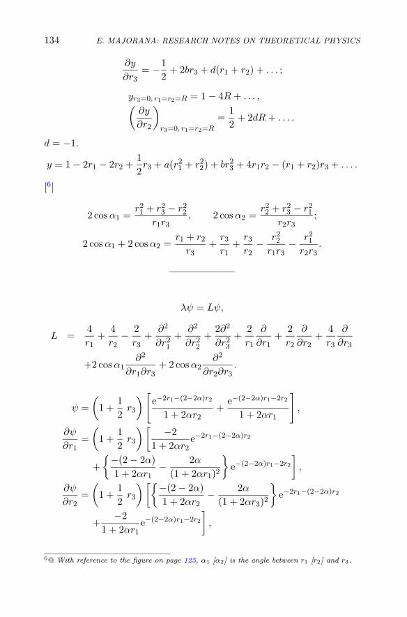
134 E. MAJORANA: RESEARCH NOTES ON THEORETICAL PHYSICS

∂y

∂r3= −1

2+ 2br3 + d(r1 + r2) + . . . ;

yr3=0, r1=r2=R = 1 − 4R + . . . ,(

∂y

∂r2

)

r3=0, r1=r2=R

=12

+ 2dR + . . . .

d = −1.

y = 1 − 2r1 − 2r2 +12r3 + a(r2

1 + r22) + br2

3 + 4r1r2 − (r1 + r2)r3 + . . . .

[6]

2 cos α1 =r21 + r2

3 − r22

r1r3, 2 cos α2 =

r22 + r2

3 − r21

r2r3;

2 cos α1 + 2 cos α2 =r1 + r2

r3+

r3

r1+

r3

r2− r2

2

r1r3− r2

1

r2r3.

——————–

λψ = Lψ,

L =4r1

+4r2

− 2r3

+∂2

∂r21

+∂2

∂r22

+2∂2

∂r23

+2r1

∂

∂r1+

2r2

∂

∂r2+

4r3

∂

∂r3

+2 cos α1∂2

∂r1∂r3+ 2 cos α2

∂2

∂r2∂r3.

ψ =(

1 +12

r3

)[e−2r1−(2−2α)r2

1 + 2αr2+

e−(2−2α)r1−2r2

1 + 2αr1

]

,

∂ψ

∂r1=

(1 +

12

r3

)[−2

1 + 2αr2e−2r1−(2−2α)r2

+{−(2 − 2α)1 + 2αr1

− 2α

(1 + 2αr1)2

}e−(2−2α)r1−2r2

],

∂ψ

∂r2=

(1 +

12

r3

)[{−(2 − 2α)1 + 2αr2

− 2α

(1 + 2αr3)2

}e−2r1−(2−2α)r2

+−2

1 + 2αr1e−(2−2α)r1−2r2

],

6@ With reference to the figure on page 125, α1 [α2] is the angle between r1 [r2] and r3.

ATOMIC PHYSICS 135

∂ψ

∂r3=

12

[e−2r1−(2−2α)r2

1 + 2αr2+

e−(2−2α)r1 − 2r2

1 + 2αr1

]

,

∂2ψ

∂r21

=(

1 +12

r3

)[4

1 + 2αr2e−2r1−(2−2α)r2

+{

(2 − 2α)2

1 + 2αr1+

4α(2 − 2α)(1 + 2αr1)2

+8α2

(1 + 2αr1)3

}e−(2−2α)r1−2r2

],

∂2ψ

∂r22

=(

1 +12

r3

)[{(2 − 2α)2

1 + 2αr2+

4α(2 − 2α)(1 + 2αr2)2

+8α2

(1 + 2αr2)3

}e−2r1−(2−2α)r2 +

41 + 2αr1

e−(2−2α)r1−2r2

],

∂2ψ

∂r23

= 0,

∂2ψ

∂r1∂r3=

−11 + 2αr2

e−2r1−(2−2α)r1

+{−(1 − α)1 + 2αr1

− α

(1 + 2αr1)2

}e−(2−2α)r1−2r2 ,

∂2ψ

∂r2∂r3=

{−(1 − α)1 + 2αr2

− α

(1 + 2αr2)2

}e−2r1−(2−2α)r2

+−1

1 + 2αr1e−(2−2α)r1−2r2 .

Lψ = P (r1, r2, r3)e−2r1−(2−2α)r2 + P (r2, r1, r3)e−2(2−2α)r1−2r2 ,

P =1 + r3/21 + 2αr2

{4r1

+4r2

+2r3

+ 4 + (2 − 2α)2 +4α(2 − 2α)1 + 2αr2

+8α2

(1 + 2αr2)2− 4

r1− 4 − 4α

r2− 4α

r2(1 + 2αr2)+

2r3 (1 + r3/2)

− 2 cos α1

1 + r3/2− cos α2

1 + 12r3

(2 − 2α +

2α

1 + 2αr1

)}

=1 + r3/21 + 2αr2

{4 + (2 − 2α)2 +

8α2

1 + 2αr2− 1

1 + r3/2− cos α1

1 + r3/2

− cos α2

1 + r3/2

(2 − 2α +

2α

1 + 2αr1

)}.

136 E. MAJORANA: RESEARCH NOTES ON THEORETICAL PHYSICS

3.3. CONTINUATION: WAVEFUNCTIONSFOR THE HELIUM ATOM

ψ = e−p,

p =2r1 + 2r2 −

12r3 + a(r2

1 + r22) + br1r2 + cr2

3 + d(r1 + r2)r3

1 + e(r1 + r2) + fr3.

λ =4r1

+4r2

− 2r3

+ ∇2

=4r1

+4r2

− 2r3

+∂2

∂r21

+∂2

∂r22

+ 2∂2

∂r23

+2r1

∂

∂r1+

2r2

∂

∂r2+

4r3

∂

∂r3

+2 cos α1 ·∂2

∂r1∂r3+ 2 cos α2 ·

∂2

∂r2∂r3.

α1 = OP1 − P2P1; α2 = OP2 − P1P2.

ψ0 = e−2r1−2r2+ 12r3 ;

∂

∂r1= −2,

∂

∂r2= −2,

∂

∂r3=

12,

∂2

∂r21

= 4,∂2

∂r22

= 4,∂2

∂r23

=14,

∂2

∂r1∂r2= 4,

∂2

∂r1∂r3= −1,

∂2

∂r2∂r3= −1.

λ0 =4r1

+4r2

− 2r3

+ 4 + 4 +12− 4

r1− 4

r2+

2r3

− 2 cos α1 − 2 cos α2

=172

− 2 cos α1 − 2 cos α2,

λmax0 = 8.5, λmin

0 = 4.5.

ATOMIC PHYSICS 137

2 =(

∂p

∂r1

)

r1=0,r2=r3=R

=(2 + bR + dR)(1 + eR + fR) − e

[2R − 1

2R + aR2 + cR2 + dR2]

(1 + eR + fR)2

=2 + R

(b + d + 2e+2f − 3

2e)

+R2(be+ bf + � de + df − ae− ce−� de)1 + R(2e + 2f) + R2(e2 + f2 + 2ef)

=2 + R

(b + d + 1

2e + 2f)

+ R2(−ae + be + bf − ce + df)1 + R(2e + 2f) + R2(e2 + f2 + 2ef)

.

b + d +12e + 2f = 4e + 4f,

−ae + be + bf − ce + df = 2e2 + 2f2 + 4ef ;

b + d − 72e − 2f = 0,

ac − be − bf + ce − df + 2e2 + 4ef + 2f2 = 0.

−12

=(

∂p

∂r3

)

r3=0,r1=r2=R

=

(−1

2 + 2dR)(1 + 2eR) − f(2R + 2R + aR2 + aR2 + bR2)

(1 + 2eR)2

=−1

2 + R(2d − e − 4f) + R2(4de − 2af − bf)1 + 4eR + 4e2R2

.

2d − e − 4f = −2e,

4de − 2af − bf = −2e2.

2d + e − 4f = 0,

2b + 2d − 7e − 4f = 0,

2af + bf − de − 2e2 = 0,

ae − be − bf + ce − df + 2e2 + 4ef + 2f2 = 0.

138 E. MAJORANA: RESEARCH NOTES ON THEORETICAL PHYSICS

e = A, f = B,

d = −A

2+ 2B,

b = 4A,

a = 0,

c = 2A − 12B.

p0 =2r1 +2r2 − 1

2r3 + 4Ar1r2 +(2A− 1

2B)r23 +

(2B − 1

2A)(r1 + r2)r3

1 + A(r1 + r2) + Br3.

ψ0 = e−p, ∇2 ψ0 = (−∇2 p + (∇ p)2)ψ0.

λ =4r1

+4r2

− 2r3

− ∂2p

∂r21

− ∂2p

∂r22

− 2∂2p

∂r23

− 2r1

∂p

∂r1− 2

r2

∂p

∂r2− 4

r3

∂p

∂r3

−2 cos α1∂2p

∂r1∂r3− 2 cos α2

∂2p

∂r2∂r3+

(∂p

∂r1

)2

+(

∂p

∂r2

)2

+ 2(

∂p

∂r3

)2

+2 cos α1∂p

∂r1

∂p

∂r3+ 2 cos α2

∂p

∂r2

∂p

∂r3.

p =R

S.

∂p

∂r1=

1S2

(∂R

∂r1S − dS

dr1R

),

∂p

∂r2=

1S2

(∂R

∂r2S − ∂S

∂r2R

),

∂p

∂r3=

1S2

(∂R

∂r3S − ∂S

∂r3R

).

∂2p

∂r21

=1S3

[(∂2p

∂r21

S +∂R

∂r1

∂S

∂r1− ∂S

∂r1

∂R

∂r1− ∂2S

∂r21

)S

−2(

∂R

∂r1S − ∂S

∂r1R

)∂S

∂r1

]

=1S3

[S

(∂2R

∂r21

− R∂2S

∂r21

)− 2

∂S

∂r1

(S

∂R

∂r1− R

∂S

∂r1

)];

ATOMIC PHYSICS 139

∂2p

∂r1∂r2=

1S3

[S

(∂2R

∂r1∂r2+

∂R

∂r1

∂S

∂r2− ∂S

∂r1

∂R

∂r2− R

∂2S

∂r1∂r2

)

−2∂S

∂r2

(S

∂R

∂r1− R

∂S

∂r1

)]

=1S3

[S

(∂2R

∂r1∂r2− R

∂2S

∂r1∂r2− ∂R

∂r1

∂S

∂r2− ∂R

∂r2

∂S

∂r1

)

+2R∂S

∂r1

∂S

∂r2

].

R = 2r1 + 2r2 −12r3 + 4Ar1r2 +

(2A − 1

2B

)r23

+(

2B − 12A

)(r1 + r2)r3,

S = 1 + A(r1 + r2) + Br3.

∂R

∂r1= 2+4Ar2 +

(2B − 1

2A

)r3,

∂R

∂r2= 2+4Ar1 +

(2B − 1

2A

)r3,

∂R

∂r3= −1

2+

(2B − 1

2A

)(r1 + r2) + (4A − B)r3;

∂2R

∂r21

= 0,∂2R

∂r22

,∂2R

∂r23

= 4A − B;

∂2R

∂r1∂r2= 4A,

∂2R

∂r1∂r3= 2B − 1

2A,

∂2R

∂r2∂r3= 2B − 1

2A.

∂S

∂r1= A,

∂S

∂r2= A,

∂S

∂r3= B;

∂2S

∂r21

= 0,∂2S

∂r22

= 0,∂2S

∂r23

= 0;

∂2S

∂r1∂r2= 0,

∂2S

∂r1∂r3= 0,

∂2S

∂r2∂r3= 0.

p = p0.

[7]

7@ The original manuscript then continues with some calculations aimed at evaluating thederivatives of p. In the following we report only the final results.

140 E. MAJORANA: RESEARCH NOTES ON THEORETICAL PHYSICS

∂p

∂r1= 2 +

−4Ar1 − 2A2r21 + 2A2r2

2 − 2A2r23 − 4A2r1r2 − 4ABr1r3

[1 + A(r1 + r2) + Br3]2,

∂p

∂r2= 2 +

−4Ar2 − 2A2r22 + 2A2r2

1 − 2A2r23 − 4A2r1r2 − 4ABr2r3

[1 + A(r1 + r2) + Br3]2,

∂p

∂r3=

1[1 + A(r1 + r2) + Br3]2

{[1 + a(R1 + R2) + bR3]

[−1

2

+(

2B − 12A

)(r1 + r2) + (4A − B)r3

]

−B

[2r1 + 2r2 −

12r3 + 4Ar1r2 +

(2A − 1

2B

)r23

+(

2B − 12A

)(r1 + r2)r3

]}.

——————–

ψ0 =(

1 +12r3

)e−2r1−2r2 .

∂ψ0

∂r1= −2ψ0,

∂ψ0

∂r2= −2ψ0,

∂ψ0

∂r3=

12

e−2r1−2r2 ;

∂2ψ0

∂r21

= 4ψ0,∂2ψ0

∂r22

= 4ψ0,∂2ψ0

∂r23

= 0;

∂2ψ0

∂r1∂r3= 4ψ0,

∂2ψ0

∂r1∂r3= e−2r1−2r2 ,

∂2ψ0

∂r23

= e−2r1−2r2 .

λ0 =4r1

+4r2

− 2r3

+ 4 + 4 − 4r1

− 4r2

+1

1 + 12r3

2r3

− 21 + 1

2r3cos α1 −

21 + 1

2r3cos α2

= 8 − 11 + 1

2r3− 2

1 + 12r3

(cos α1 + cos α2) ,

λmax0 = 8, λmin

0 = 3.

——————–

ATOMIC PHYSICS 141

λψ = Lψ, L =4r1

+4r2

− 2r3

+ ∇2 .

χ =√

r1r2r3 ψ.

λχ = L′χ =√

r1r2r3 Lψ,

L′ =√

r1r2r3 L1

√r1r2r3

.

L′ =4r1

+4r2

− 2r3

+(

∂2

∂r21

− 1r1

∂

∂r1+

34r2

1

)+

(∂2

∂r22

− 1r2

∂

∂r2+

34r2

2

)

+(

2∂2

∂r23

− 2r3

∂

∂r3+

32r2

3

)+

(2r1

∂

∂r1− 1

r21

)

+(

2r2

∂

∂r2− 1

r23

)+

(4r3

∂

∂r3− 2

r33

)

+2 cos α1

(∂2

∂r1∂r3− 1

2r1

∂

∂r3− 1

2r3

∂

∂r1+

14r1r3

)

+2 cos α2

(∂2

∂r2∂r3− 1

2r2

∂

∂r3− 1

2r3

∂

∂r2+

14r2r3

).

∂

∂r1

1√

r1= − 1

2r

1√

r1,

∂2

∂r21

1√

r1=

34r2

1√

r1,

∂2

∂r1∂r3

1√

r1r3=

14r1r3

.

∂2

∂r21

−→ ∂2

∂r21

− 1r1

∂

∂r1+

34r2

1

,

∂

∂r1−→ ∂

∂r1− 1

2r1,

∂2

∂r1∂r3−→ ∂2

∂r1∂r3− 1

2r1

∂

∂r3− 1

2r3

∂

∂r1+

14r1r3

.

3.4. SELF-CONSISTENT FIELD INTWO-ELECTRON ATOMS

A self-consistent field method is here applied to the problem of two-electron atoms with nuclear charge Z. The quantities r1 and r2 are

142 E. MAJORANA: RESEARCH NOTES ON THEORETICAL PHYSICS

the distance of the two electrons from the nucleus, while r12 denotes theinter-electron distance.

Eϕ = Hϕ =(−2

Z

r1− 2

Z

r2+

2r12

)ψ − ∇2 ϕ.

W =

∫ϕHψdτ∫

ϕ2dτ

.

δ

∫ϕ(H − W ′)ϕdτ = 0.

∫ϕ(H − W )ϕdτ = 0,

δϕ = αϕ:

δ

∫ϕ(H − W ′)ϕdτ = 2α

∫ϕ(H − W ′)ϕdτ = 0;

W ′ = W.

——————–

δ

∫ϕ(H − W )ϕdτ = 0. (1)

ϕ(r1, r2, r12) = y(r1)y(r2),

δϕ = y(r1)δy(r2) + y(r2)δy(r1).

δ

∫ϕ(H − W )ϕdτ

= 2∫

[y(r1)δy(r2) + y(r2)δy(r1)](H − W )y(r1)y(r2)dτ

= 4∫

y(r2)δy(r1)(H − W )[y(r1)y(r2)]dq2 = 0 (2)

= −2Z

r1y(r1)y(r2) − y(r1)

2Z

r2y(r2) + y(r1)

z

r12y(r2) − y(r1)∇2 y(r2)

− ∇2 y(r1) · y(r2) − Wy(r1)y(r2),

ATOMIC PHYSICS 143

δ

∫ϕ(H − W )ϕdτ = 4

∫δy(r1)

{[−2Z

r1−

∫2Zy2(r1)

r2dq2

+∫

2y2(r2)r12

dq2 −∫

y(r2)∇2 y(r2)dτ − W

]

−∇2 y(r1)}

dq1.

[−2Z

r1−

∫2Zy2(r2)

r2dq2 +

∫2y2(r2)

r12dq2

−∫

y(r2)∇2 y(r2)dq2 − W

]y(r1) − ∇2 y(r1) = 0,

[−2Z

r2−

∫2Zy2(r1)

r1dq1 +

∫2y2(r1)

r12dq1

−∫

y(r1)∇2 y(r1)dq1 − W

]y(r2) − ∇2 y(r2) = 0.

∫ [−2Zy2(r2)

r2+ y(r2)∇2 y(r2)

]dq2 = A

=∫ [

−2Zy2(r2)r1

− y(r1)∇2 y(r2)]

dq1.

(−2Z

r1+

∫2y2(r2)

r12dq2 − W + A

)y(r1) − ∇2 y(r1) = 0,

(W − A)y(r1) =(−2z

r1+

∫2y2(r2)

r12dq2

)y(r1) − ∇2 y(r1).

W − A = B, r1 = r:

By(r) =(−2Z

r1+

∫2y2(r2)

r12dq2

)y(r) − d2y

dr2− 2

r

dy

dr;

B = −2Z

r1+

∫2y2(r2)

r12dq2 −

1yy′′ − 2

ryy′.

P = ry:

B = −2Z

r+

∫2y2(r2)

r12dq2 −

P ′′

P.

144 E. MAJORANA: RESEARCH NOTES ON THEORETICAL PHYSICS

0 = −8πP 2

r2− 1

r

d2

dr2

rP ′′

P,

8πP 2 + rd2

dr2

rP ′′

P= 0,

−8πP 2 = r

[ddr

(rP ′′′ + P ′′

P− rP ′′P ′

P 2

)]

= r

[rP ′′′′ + 2P ′′′

P− 2P ′P ′′ − 2rP ′P ′′′ − rP ′′2

P 2+

2rP ′2P ′′

P 2

].

3.5. 2s TERMS FOR TWO-ELECTRONATOMS

An approximate expression for the energy (in rydbergs) W (which isequal to half the mean value of the potential energy) of the 2s terms oftwo-electron atoms with charge Z is given. For further details, see Sect.15 of Volumetto III.

−W =54Z2 − 34

81± 32

729Z = Z2 +

14Z2 +

306 ∓ 32729

Z

=

⎧⎪⎪⎪⎪⎪⎪⎨

⎪⎪⎪⎪⎪⎪⎩

Z2 +14Z2 − 0.3759Z = Z2 +

14(Z2 − 1.5034Z),

for ortho-states,

Z2 +14Z2 − 0.4636Z = Z2 +

14(Z2 − 1.8546Z),

for para-states.

3.6. ENERGY LEVELS FORTWO-ELECTRON ATOMS

In the following pages, the author evaluates the energies for a number ofterms in two-electron atoms, by using certain expressions for the corre-sponding wavefunctions. The numerical values are grouped in few tables.

ATOMIC PHYSICS 145

rψ1 = y1ϕm1 (m = 1, 0,−1),

rψ2 = y2ϕm′1 (m′ = 1, 0,−1).

dτ =dxdydz

4π.

ϕ11ϕ

11 = ϕ1

1ϕ−11 = 1 − 1√

5ϕ0

2,

ϕ01ϕ

01 = (ϕ0

1)2 = 1 +

2√5ϕ0

2.

For y1ϕ11:

V (r2) =1r2

∫ r2

0y21dr1 +

∫ ∞

r2

1r1

y21dr1

−(

15√

5r31

∫ r2

0r21y

21dr1 +

r22

5√

5

∫ ∞

r2

1r31

y21dr1

)

ϕ02.

For y1ϕ01:

V (r2) =1r2

∫ r1

0y21dr1 +

∫ ∞

r2

1r1

y21dr1

+

(2

5√

5r32

∫ r2

0r21y

21dr1 +

2r22

5√

5

∫ ∞

r2

1r31

y21dr1

)

ϕ02.

A =∫

y21y

22

ridr1dr2,

B =∫

r2ky

21y

22

r3i

dr1dr2,

with ri ≥ rk.

146 E. MAJORANA: RESEARCH NOTES ON THEORETICAL PHYSICS

Electrostatic energy

y1ϕ11 y1ϕ

01 y1ϕ

−11

y2ϕ11 A +

125

B A − 225

B A +125

B

y2ϕ02 A − 2

25B A +

425

B A − 225

B

y2ϕ−12 A +

125

B A − 225

B A +125

B

� Electrostatic energy

2 A +125

B

1 A − 15B

0 A +25B

E2 = S,E1 + E2 = 2T, E1 = 2T − S,E0 + E1 + E2 = 2S + R, E0 = 2S + R − 2T.

2p2p 1D : A +125

B1Z

A =93512

4Z

=93128

= 0.181640625 = 0.72656253P : A − 1

5B

Z → ∞one electron

1S : A +35B

1Z

B =45512

4Z

B =45128

= 0.08789005 = 0.3515625

ATOMIC PHYSICS 147

1D A +125

B =2371280

= 0.18515625

Z = 1 3P A − 15B =

21128

= 0.1640625

1S A +25B =

111512

= 0.216796875

For y = x2e−12x, y2 = x4e−x, N = 24 we have in fact:

A =1

N2

∫y21y

22

xidx1dx2 =

2N2

∫ ∞

0y21dx1

∫ ∞

x1

y22

x2dx2,

∫y22

x2dx2 =

∫x3

2e−x2dx2 = −(x3

2 + 3x22 + 6x2 + 6)e−x2 ,

∫ ∞

x1

y22

x2dx2 = (x3

1 + 3x21 + 6x1 + 6)e−x1 ,

N2A = 2∫ ∞

0(x7

1 + 3x61 + 6x5

1 + 6x41)e

−2x1dx1

= 2(

7!28

+ 36!27

+ 65!26

+ 64!25

)=

3158

+1354

+452

+ 9 =8378

,

A =837

8 · 576=

938 · 64

=93512

.

B =1

N2

∫x2

1y21y

22

x3i

dx1dx2 =2

N2

∫ ∞

0x2

1y21dx1

∫ ∞

x1

y22

x32

dx2,

∫y22

x32

dx2 =∫

x2e−x2dx2 = −(x2 + 1)e−x2 ,

∫ ∞

x1

y22

x32

dx2 = (x1 + 1)e−x1 ,

N2B = 2∫ ∞

0(x7

1 + x61)e

−2x1dx1

= 2(

7!28

+6!27

)=

3158

+454

=4058

= 50.625,

148 E. MAJORANA: RESEARCH NOTES ON THEORETICAL PHYSICS

B =405

8 · 576=

458 · 64

=45512

.

2s2s 1Σ : As1Z

As =77512

4Z

As =77128

= 0.150390625 = 0.6015625

For y = (x2 − 2x)e−12x, y2 = (x4 − 4x3 + 4x2)e−x, N = 24 − 24 + 8 we

have in fact:

A =1

N2

∫y21y

22

xidx1dx2 =

2N2

∫ ∞

0y21dx1

∫ ∞

x1

y22

x2dx2,

∫y22

x2dx2 =

∫(x3

2 − 4x22 + 4x2)e−x2dx2 = −(x3

2 − x22 + 2x2 + 2)e−x2 ,

∫ ∞

x1

y22

x2dx2 = (x3

1 − x21 + 2x1 + 2)e−x1 ,

N2A = 2∫ ∞

0(x4

1 − 4x31 + 4x2

1)(x31 − x2

1 + 2x1 + 2)e−2x1dx1

= 2∫ ∞

0(x7

1 − 5x61 + 10x5

1 − 10x41 + 8x2

1)e−2x1dx1

= 2(

7!256

− 56!

128+ 10

5!64

− 104!32

+ 82!8

)

=3158

− 2254

+752

− 15 + 4 =778

= 9.625.

3.6.1 Preliminaries For The X And Y Terms

(2s)2 1S + 2p2p 1S = X + Y .

dτ1 =dx1dy1dz1

4π, dτ = dτ1dτ2.

ATOMIC PHYSICS 149

2p2p 1S :

(2s)2 1S :

u = (x1x2 + y1y2 + z1z2)e−12(z1+z2);

v = (r1 − 2)(r2 − 2)e−12(r1+r2);

uv = (x1x2 + y1y2 + z1z2)(r1r2 − 2r1 − 2r2 + 4)e−r1−r2 .

∫u2dτ =

∫(x1x2 + y1y2 + z1z2)2e−r1−r2dτ

= 3∫

x21x

22e

−r1−r2dτ

= 3(∫

x21e

r1dτ1

)2

=13

(∫r21e

−r1dτ1

)2

=13

(∫r41e

−r1dr1

)2

=13

242 = 192,

∫v2dτ =

(∫(r2

1 − 4r1 + 4)e−r1dτ1

)2

=(∫

(r41 − 4r3

1 + 4r21)e

−r1dr1

)2

= 64.

∫uv

r12= 2

∫dτ1

∫

r2>r1

uv

r12dτ2,

∫

r2>r1

uv

r12dτ2 =

13

r21 e−r1

∫ ∞

r1

r2(r1r2 − 2r1 − 2r2 + 4)e−r2dr2

=13

r21 e−2r1

[r1(r2

1 + 2r1 + 2) − 2r1(r1 + 1)

−2(r21 + 2r1 + 2) + 4(r1 + 1)

],

∫uv

r12dτ = 2

∫ ∞

0

(13r41 −

23r61

)e−2r1dr1

= 2(

13

7!28

− 23

6!27

)=

1058

− 152

=458

:

150 E. MAJORANA: RESEARCH NOTES ON THEORETICAL PHYSICS

1√NuNv

∫uv

r12dτ =

164√

3458

=15√

3512

= 0.050743676003.

77512

15√

3512

15√

3512

111512

.

a − E c

c b − E,

E2 − (a + b)E + ab − c2 = 0,

E =a + b

2±

√(a − b

2

)2

+ c2.

a + b

2=

47256

, −a − b

2=

17512

,

(a − b

2

)2

=172

5122=

2895122

, c2 =6755122

,

(a − b

2

)+

c2 =964

(512)2,

√(a − b

2

)2

+ c2 =√

964(512)2

.

E1 =94 −

√964

512=

47 −√

241256

,

E2 =94 +

√964

512=

47 +√

241256

.

X E1 = 0.12295244347 −

√241

256

Y E2 = 0.24423505747 +

√241

256

E1 + E2 = 0.3671975 =47128

.

ATOMIC PHYSICS 151

a − E1 c

c b − E1

=

−17 +√

964512

15√

3512

15√

3512

17 +√

964512

=0.027438182 0.050743676

0.050743676 0.093844432,

a − E2 c

c b − E2

=

−17 −√

964512

15√

3512

15√

3512

17 −√

964512

=0.093844432 0.050743676

0.050743676 0.027438182.

X =√

p1 (2s)2 1S −√p2 2p2p 1S,

Y =√

p2 (2s)2 1S +√

p1 2p2p 1S,

p1 + p2 = 1.

p1 =675

1928 − 34√

964=

964 + 17√

9641928

= 0.774,

p2 =675

1928 + 34√

964=

964 − 17√

9641928

= 0.226.

3.6.2 Simple Terms

2s2s 2s2p1 2s2p0 2s2p−1

2p12s 2p12p1 2p12p0 2p12p−1

2p02s 2p02p1 2p02p0 2p02p−1

2p−12s 2p−12p1 2p−12p0 2p−12p−1

——————–

152 E. MAJORANA: RESEARCH NOTES ON THEORETICAL PHYSICS

m = 2singlets

2p12p1

2p12p1

∣∣∣∣

2371280

∣∣∣∣

2p2p 1D =2371280

——————–

m = 1singlets 2s2p1

2p12p0

2s2p1 2p12p0

0

02371280

2p2p 1D =2371280

——————–

m = 1triplets 2s2p1

2p12p0

2s2p1 2p12p0

17128

0

021128

2s2p 3P =17128

2p2p 3P =21128

——————–

m = 0singlets

2s2p0

2s2s

2p12p−1

2p02p0

2s2p0 2s2s 2p12p−1 2p02p0

49256

0 0 0

077512

15√

2512

15512

015√

2512

33160

27√

22560

015512

27√

22560

5012560

With a suitable change of states:

ATOMIC PHYSICS 153

2p2p 1D =

√132p12p−1 −

√232p02p0,

2p2p 1S =

√232p12p−1 +

√132p02p0,

we have:8

2s2p0

2s2s

2p2p 1D

2p2p 1S

2s2p0 2s2s 2p2p 1D 2p2p 1S

49256

0 0 0

077512

015

√3

512

0 02371280

0

015

√3

5120

111512

2p2p1D =2371280

X =47 −

√241

256[(2s)2 1S

],

Y =47 +

√241

256[2p2p 1S

],

[9]——————–

m = 0triplets 2s2p0

2p12p−1

2s2p0 2p12p−1

0

021128

2p2p 3P =21128

——————–

8@ In the table below we have preferred to denote with the shorthand notations 2p2p 1D and2p2p 1S (used even elsewhere in the original manuscript) what the author reported in the fullexpressions given above.9@ With X and Y the author denotes the eigenvalues of the subsystem formed by 2s2s and

2p2p 1S =q

232p12p−1 +

q

132p02p0.

154 E. MAJORANA: RESEARCH NOTES ON THEORETICAL PHYSICS

2p2p 1D :2371280

= 0.185.156.250;

2p2p 3P :21128

= 0.164.062.500;

2s2p 3P :17128

= 0.132.812.500;

2s2p 1P :49256

= 0.191.406.250;

−√p2 2s2s 1S +

√p1 2p2p 1S = Y :

47 +√

241256

= 0.244.235.057;

√p1 2s2s 1S +

√p2 2p2p 1S = X :

47 −√

241256

= 0.122.952.443.

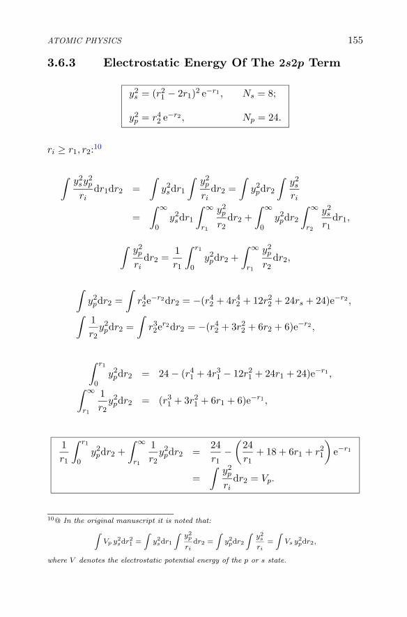
ATOMIC PHYSICS 155

3.6.3 Electrostatic Energy Of The 2s2p Term

y2s = (r2

1 − 2r1)2 e−r1 , Ns = 8;

y2p = r4

2 e−r2 , Np = 24.

ri ≥ r1, r2:10

∫y2

sy2p

ridr1dr2 =

∫y2

sdr1

∫y2

p

ridr2 =

∫y2

pdr2

∫y2

s

ri

=∫ ∞

0y2

sdr1

∫ ∞

r1

y2p

r2dr2 +

∫ ∞

0y2

pdr2

∫ ∞

r2

y2s

r1dr1,

∫y2

p

ridr2 =

1r1

∫ r1

0y2

pdr2 +∫ ∞

r1

y2p

r2dr2,

∫y2

pdr2 =∫

r42e

−r2dr2 = −(r42 + 4r4

2 + 12r22 + 24rs + 24)e−r2 ,

∫1r2

y2pdr2 =

∫r32e

r2dr2 = −(r42 + 3r2

2 + 6r2 + 6)e−r2 ,

∫ r1

0y2

pdr2 = 24 − (r41 + 4r3

1 − 12r21 + 24r1 + 24)e−r1 ,

∫ ∞

r1

1r2

y2pdr2 = (r3

1 + 3r21 + 6r1 + 6)e−r1 ,

1r1

∫ r1

0y2

pdr2 +∫ ∞

r1

1r2

y2pdr2 =

24r1

−(

24r1

+ 18 + 6r1 + r21

)e−r1

=∫

y2p

ridr2 = Vp.

10@ In the original manuscript it is noted that:

Z

Vp y2sdr2

1 =

Z

y2sdr1

Z

y2p

ridr2 =

Z

y2pdr2

Z

y2s

ri=

Z

Vs y2pdr2,

where V denotes the electrostatic potential energy of the p or s state.

156 E. MAJORANA: RESEARCH NOTES ON THEORETICAL PHYSICS

∫y2

sVpdr1 =∫ ∞

0

[(24r3

1 − 96r21 + 96r1)er1

−(r61 + 2r5

1 − 2r41 − 24r3

1 − 24r21 + 96r1

)e−2r1

]dr1

= 144 − 192 + 96 − 720128

+24064

+4832

+14416

+488

− 964

.

1NsNp

∫y2

sy2p

ridr1dr2 =

34− 1 +

12− 15

512− 5

256+

1128

+364

+132

− 18

=83512

= M.

32y2

s − 12y2

p = 12

(y2

s

N2s

−y2

p

N2p

)

= (r41 − 6r3

1 + 6r21)e

−r1 = t1.

∫t1t2ri

dr1dr2 = 2∫ ∞

0t1dr1

∫ ∞

r1

t2r2

dr2,

∫t2r2

dr2 =∫

(r32 − 6r2

2 + 6r2)e−r2dr2 = −(r32 − 3r2

2)e−r2 .

Es + Ap − 2M =1

144

∫t1t2ri

dr1dr2

=172

∫ ∞

0(r4

1 − 6r31 + 6r2

1)(r31 − 3r2

1)e−2ridr1

=∫ ∞

0(r7

1 − 9r61 + 24r5

1 − 18r41)e

−2r1dr1

=172

(5040256

− 9 · 720128

+24 · 120

64− 18 · 24

32

)

=35128

− 4584

+58− 3

16=

1128

.

Es =77512

; Ap =93512

;

M =Es + Ap

2− 1

256=

83512

= 0.162109375.

ATOMIC PHYSICS 157

3.6.4 Perturbation Theory For s Terms

ψ = er1−r2 .

H0 = − 1r1

− 1r2

− 12∇2

1 −12∇2

2.

H0ψ0 =[− 1

r1− 1

r2−

(12− 1

r1

)−

(12− 1

r2

)]ψ0 = −ψ0.

Then: E0 = −1. For λ → 0:

H = H0 + λH1, H1 =1

r12.

ψ = ψ0 + λψ1 + λ2ψ2 + . . . ,

E = E0 + λE1 + λ2E2 + . . . .

0 = (H − E)ψ= (H0 + λH1 − E0 − λE1 − λ2E2 . . .)(ψ0 + λψ1 + λ2ψ + . . .)

=

(

H0 + λH1 −∞∑

i=0

λiEi

) ∞∑

k=0

λkψk;

(H0 − E0)ψn = (E1 − H1)ψn−1 + E2ψn−2 + E3ψn−3 + . . . + Enψ0.

(H0 − E0)ψ0 = 0,

(H0 − E0)ψ1 = (E1 − H1)ψ0,

E1 =58.

By setting:

ψ1 = y e−r1−r2 ,

158 E. MAJORANA: RESEARCH NOTES ON THEORETICAL PHYSICS

we have:

∇2 ψ1 =(

2 − 2r1

− 2r2

)y e−r1−r2−2

(∂y

∂r1+

∂y

∂r2

)e−r1−r2+∇2 y e−r1−r2 ,

(H0 − E0)ψ1 =(

1 − 1r1

− 1r2

− 12∇2

)ψ1

=(

∂y

∂r1+

∂y

∂r2+

12− 1

2y

)e−r1−r2 =

(58− 1

r12

)er1−r2 ,

∂y

∂r1+

∂y

∂r2− 1

2∇2 y =

58− 1

r12.

y =∞∑

�=0

P�(cos θ) fl(r1, r2).

3.6.5 2s2p 3P TermLet us consider the functions:

(r1 − 2)e−12r1 , r2e−

12r2 .

ψ = e−12(r1+r2)

[(r1 − 2)r2ϕ

01(q2) − (r2 − 2)r1ϕ

02(q1)

],

ψ2 = e−(r1+r2){(r1 − 2)2r2

2 + (r2 − 2)2r21

−2r1r2(r1 − 2)(r2 − 2)ϕ01(q1)ϕ0

1(q2)

+2√5(r1 − 2)2r2

2ϕ02(q2) +

2√5(r2 − 2)2r2

1ϕ02(q1)

},

where we have used: ϕ012 = 1 +

2√5ϕ0

2.

N = 384 = 2 · 8 · 24.

ATOMIC PHYSICS 159

43

∫ ∞

0(r5

1 − 2r4)er1dr1

∫ ∞

r1

r2(r2 − 2)e−r2dr2

=43

∫ ∞

0(r7

1 − 2r61)e

−2r1dr1 =454

.

Isp =45

4 · 384=

15512

.

3.6.6 X TermZ = 2.

dτ =dxdydz

4π.

[11]

y1 = r1r2e−r1−r2 ,

y2 = (r1 + r2)e−r1−r2 ,

y3 = e−r1−r2 ,

y4 = (x1x2 + y1y2 + z1z2)e−r1−r2 .

∫y21 dτ =

(∫ ∞

0r41e

−2r1dr1

)2

=(

2432

)2

=916

,

∫y22 dτ = 2

∫ ∞

0r41e

−2r1dr1

∫ ∞

0r22e

−2rdr2 + 2(∫ ∞

0r31e

2r1dr1

)2

,

= 2 · 34· 14

+ 2 ·(

38

)2

=2132

,

∫y23 dτ =

(∫ ∞

0r21e

−2r1dr1

)2

=(

14

)2

=116

,

∫y24 dτ =

13

(∫r41e

−2r1dr1

)2

=13

(34

)2

=316

,

∫y1y2 dτ = 2

∫ ∞

0r41e

2r1dr1

∫ ∞

0r32e

−2r2dr2 = 2 · 34· 38

=916

,

11@ Remember that the X term is a superposition of the 2s2s 1S and 2p2p 1S ones.

160 E. MAJORANA: RESEARCH NOTES ON THEORETICAL PHYSICS

∫y1y3 dτ =

(∫ ∞

0r31e

−2r1dr1

)2

=(

38

)2

=964

,

∫y2y3 dτ = 2

∫r31e

−2r1dr1

∫r22e

−2r2dr2 = 2 · 38· 14

=316

.

Kinetic energy: T = −12∇2 .

Potential energy: U = − 2r1

− 2r2

+1r3

.

∇21 r1e−r1 =

(r1 − 4 +

2r1

)er1 =

(1 − 4

r1+

2r21

)r1e−r1 ,

−12∇2

1 r1e−r1

(−r1

2+ 2 − 1

r1

)e−r1 =

(−1

2+

2r1

− 1r21

)r1e−r1 .

∫y1Ty1 dτ = 2

∫ ∞

0

(−r4

1

2+ 2r3

1 − r21

)e−2r1dr1

∫ ∞

0r42e

−2r2dr2

= 2 ·(−3

8+

34− 1

4

)· 34

=316

,

∫y2Ty1 dτ = 2

∫ ∞

0

(−r4

1

2+ 2r3

1 − r21

)e−2r1dr1

∫ ∞

0r32e

−2r2dr2

+2∫ ∞

0

(−r3

1

2+ 2r2

1 − r1

)e−2r1dr1

∫ ∞

0r43e

−2r2dr1

= 2 · 18· 38

+ 2(− 3

16+

12− 1

4

)· 34

=332

+332

=316

.

−12∇2 r1e−r1 =

(−r1

2+ 2 − 1

r1

)e−r1 ,

−12∇2 r1e−r1 =

(−1

2+

1r1

)e−r1 ,

T y2 =(−r1

2+ 2 − 1

r1

)e−r1−r2 +

(−1

2+

1r1

)r2e−r1−r2 .

∫y1Ty2 dτ = 2

∫ ∞

0

(−r4

1

2+ 2r3

1 − r31

)e−2r1dr1

∫ ∞

0r32e

−2r1dr2

+2∫ ∞

0

(−1

2r31 + r2

1

)e−2r1dr1

∫ ∞

0r42e

−2r1dr2

= 2 · 18· 38

+ 2 · 116

· 34

=316

,

ATOMIC PHYSICS 161

∫y3Ty1 dτ = 2

∫ ∞

0

(−r3

1

2+ 2r2

1 − r1

)e−2r1dr1

∫ ∞

0r32e

−2r2dr2

= 2 · 116

· 38,

∫y4Ty dτ = 0,

∫y2Ty2 dτ = 2

∫ ∞

0

(−r4

1

2+ 2r2

1 − r21

)e−2r1dr1

∫ ∞

0r22e

−2r2dr2

+2∫ ∞

0

(−r3

1

2+ r2

1

)e−2r1dr1

∫ ∞

0r32e

−2r2dr2

+2∫ ∞

0

(−r3

1

2+ 2r2

1 − r1

)e−2r1dr1

∫ ∞

0r32e

−2r2dr2

+2∫ ∞

0

(−r2

1

2+ r1

)e−2r1dr1

∫ ∞

0r42e

−2r2dr2

= 2 · 18· 14

+ 2 · 116

· 38

+ 2 · 116

· 38

+ 2 · 18· 34

=116

+364

+364

+316

=1132

,

∫y2Ty3 dτ = 2

∫ ∞

0

(−r3

1

2+ r2

1

)e−2r1dr1

∫ ∞

0r22e

−r2dr2

+2∫ ∞

0

(−r2

1

2+ r1

)e−2r1dr1

∫ ∞

0r32e

−2r2dr2

= 2 · 116

· 14

+ 2 · 18· 38

=132

+332

=18,

∫y3Ty3 dτ = 2

∫ ∞

0

(−r2

1

2+ r1

)e−2r1dr1

∫ ∞

0r22e

−r2dr2

= 2 · 18· 14

=116

.

T1(x1x2 + y1y2 + z1z2)e−r1−r2

= (x1x2 + y1y2 + z1z2)(−1

2+

1r1

)e−r1−r2

+ (x1x2 + y1y2 + z1z2)1r1

e−r1−r2 .

162 E. MAJORANA: RESEARCH NOTES ON THEORETICAL PHYSICS

∫y4Ty4 dτ = 2

∫(x1x2 + y1y2 + r1r2)2

(−1

2+

2r1

)e−2r1−2r2dτ

=23

∫ ∞

0

(−r4

1

2+ 2r3

1

)e−2r1dr1

∫ ∞

0r42e

−r2dr

=23· 38· 34

=316

.

∫y1Uy1 dτ = −4

∫ ∞

0r31e

−2r1dr1

∫ ∞

0r42e

−2r1dr2

+2∫ ∞

0r41e

−2r1dr1

∫ ∞

r1

r32e

−2r2dr2

= −4 · 38· 34

+ 2 · 8378192

= −98

+8374096

= −37714096

,

given that:∫

r32e

−2r2dr2 = −(

12r32 +

34r22 +

34r2 +

38

)e−2r2 ,

∫ ∞

r1

r32e

−2r2dr2 =(

12r31 +

34r21 +

34r1 +

38

)e−2r1 ,

∫ ∞

0

(12r71 +

34r61 +

34r51 +

38r41

)e4r1dr1

=12

50404096 · 16

+34

7201024 · 16

+34

1204096

+38

241024

=3158192

+1354096

+45

2048+

91024

=8378192

.

∫Uy1 y2 dτ = −4

∫ ∞

0r31e

−2r1dr1

∫ ∞

0r32e

−2r2dr2

−4∫ ∞

0r41e

−2r1dr1

∫ ∞

0r22e

−2r2dr2

+2∫ ∞

0r41e

−2r1dr

∫ ∞

r1

r22e

−2r2dr2

+2∫ ∞

0r32e

−2r2dr2

∫ ∞

r2

r31e

−2r1dr1

= −4 · 38· 38− 4 · 3

4· 14

+ 2 · 872048

+ 2 · 9128

= − 916

− 34

+87

1024+

964

= −11131024

,

ATOMIC PHYSICS 163

because:∫ ∞

r1

r22e

−2r2dr2 =(

12r21 +

12r1 +

14

)e−2r1 ,

∫ ∞

r2

r31e

−2r1dr1 =(

12r32 +

34r22 +

34r2 +

38

)e−2r2 ,

∫ ∞

0

(12r61 +

12r51 +

14r41

)e−4r2dr1

=12

72016384

+12

1204096

+14

241024

=87

2048,

∫ ∞

r2

(12r62 +

34r52 +

34r42 +

38r32

)e−4r2dr2

=12

72016384

+34

1204096

+34

241024

+38

9256

=9

128.

∫y3 y1 U dτ = −4

∫ ∞

0r21e

−2r1dr1

∫ ∞

0r22e

−2r2dr2

+2∫ ∞

0r31e

−2r1dr1

∫ ∞

r1

r22e

−2r2dr2

= −4 · 12· 38

+ 2 · 331024

= −38

+33512

= −159512

,

since:∫ ∞

r1

r22e

−2r2dr2 =(

12r21 +

12r1 +

14

)e−2r1 ,

∫ ∞

0

(12r51 +

12r41 +

14r31

)e−4r2dr1

=12

1204096

+12

241024

+14

6256

=15

1024+

3256

+3

512=

331024

.

∫U y2 y2 dτ = −12

∫ ∞

0r31e

−2r1dr1

∫ ∞

0r22e

−2r2dr2

−4∫ ∞

0r1e−2r1dr1

∫ ∞

0r32e

−2r2dr2

+2∫ ∞

0r41e

−2r1dr1

∫ ∞

r1

r2e−2r2dr2

+2∫ ∞

0r22e

−2r2dr2

∫ ∞

r2

r31e

−2r1dr2

+4∫ ∞

0r31e

−2r1dr1

∫ ∞

r1

r22e

−2r2dr2

164 E. MAJORANA: RESEARCH NOTES ON THEORETICAL PHYSICS

= −12 · 38· 14− 4 · 1

4· 34

+ 2 · 211024

+ 2 · 631024

+ 4 · 331024

= −98− 3

4+

21512

+63512

+33256

= −158

+95256

= −405256

,

because:

∫ ∞

r1

r2e−2r2dr2 =(

12r1 +

14

)e−2r1 ,

∫ ∞

0

(12r51 +

14r41

)e−4r2dr1

=12

1204096

+14

241024

=15

1024+

3512

=21

1024,

∫ ∞

r2

r31e

−2r1dr1 =(

12r32 +

34r22 +

34r2 +

38

)e−2r2 ,

∫ ∞

0

(12r32 +

34r22 +

34r2 +

38

)e−4r2dr2

=12

1204096

+34

241024

+34

6256

+38

264

=15

1024+

9512

+9

512+

3256

=63

1024,

∫ ∞

r1

r22e

−2r2dr2 =(

12r21 +

12r1 +

14

)e−2r1 ,

∫ ∞

0

(12r21 +

12r1 +

14

)e−4r1dr1

=12

1204096

+12

241024

+14

6256

=15

1024+

3256

+3

512=

331024

.

∫U y3 y2 dτ = −4

∫ ∞

0r21e

−2r1dr1

∫ ∞

0r22e

−2r2dr2

−4∫ ∞

0r31e

−2r1dr1

∫ ∞

0r2e−2r2dr2

+2∫ ∞

0r22e

−2r2dr2

∫ ∞

r2

r21e

−2r2dr1

+2∫ ∞

0r31e

−2r1dr1

∫ ∞

r1

r2e−2r2dr2

ATOMIC PHYSICS 165

= −4 · 14· 14− 4 · 3

8· 14

+ 2 · 132

+ 2 · 9512

= −58

+25256

= −135256

,

given that:

∫ ∞

r2

r21e

−2r1dr1 =(

12r22 +

12r2 +

14

)e−2r2 ,

∫ ∞

0

(12r22 +

12r2 +

14

)e−4r2dr2

=12

241024

+12

6256

+14

264

=132

,∫ ∞

r1

r2e−2r2dr2 =(

12r1 +

14

)e−2r1 ,

∫ ∞

0

(12r41 +

14r31

)e−2r1dr1 =

12

241024

+14

6256

=9

512.

∫y3 U y3 dτ = −4

∫ ∞

0r1e−2r1dr1

∫ ∞

0r22e

−2r2dr2

+2∫ ∞

0r21e

−2r1dr1

∫ ∞

0r2e−2r2dr2

= −4 · 14· 14

+ 2 · 5256

= −14

+5

128= − 27

128,

because:

∫ ∞

r1

r2e−2r2dr2 =(

12r1 +

12

)e2r1 ,

∫ ∞

0

(12r31 +

14r21

)e−4r1dr1 =

12

6256

+14

264

=5

256.

∫y4 U y1 dτ =

23

∫ ∞

0r41e

−2r1dr1

∫ ∞

r1

r22e

−2r2dr2

=23· 5558192

=1854096

,

166 E. MAJORANA: RESEARCH NOTES ON THEORETICAL PHYSICS

since:∫ ∞

r1

r22e

−2r2dr2 =(

12r21 +

12r1 +

14

)e−2r1 ,

∫ ∞

0

(12r71 +

12r61 +

14r51

)e−4r1

=12

504064 · 1024

+12

72016 · 1024

+14

1204 · 1024

=3158192

+45

2048+

152048

=5558192

.

∫U y2 y4 dτ =

∫1

r12y2 y4 dτ

=23

∫ ∞

0r51e

−2r1dr1

∫ ∞

r1

r2e−2r2dr2

+23

∫ ∞

0r42e

−2r2dr2

∫ ∞

r1

r21e

−2r1dr1

=23· 15512

+23· 872048

=5

256+

291024

=49

1024,

given that:∫ ∞

0

(12r61 +

14r51

)e−4r1dr1

=12

72016384

+14

1204096

=45

2048+

152048

=15512

,∫ ∞

0

(12r61 +

12r51 +

14r41

)e−4r1dr1

=12

72016384

+12

1204096

+14

241024

=45

2048+

151024

+3

512=

872048

.

∫1

r12y3 y4 dτ =

23

∫ ∞

0r41e

−2r1dr1

∫ ∞

r1

r2e−2r2dr2 =7

512,

because:∫ ∞

0

(12r51 +

14r41

)e−4r1r1

=12

1204096

+14

241024

=15

1024+

3512

=21

1024.

ATOMIC PHYSICS 167

∫U y2

4 dτ = −43

∫ ∞

0r31e

−2r1dr1

∫ ∞

0r42e

−2r2dr2

+23

∫ ∞

0r41e

−2r1dr1

∫ ∞

r1

r32e

−2r2dr2

+415

∫ ∞

0r61e

−2r1dr1

∫ ∞

r1

r2e−2r2dr2

= −43· 38· 34

+23· 8378192

+415

4058192

= −38− 879

4096+

272048

= −38

+3334096

= −12034096

,

since:∫ ∞

0

(12r71 +

34r61 +

34r51 +

38r41

)e−4r1dr1

=12

504064 · 1024

+34

72016 · 1024

+120

4 · 1024+

38

241024

=3158192

+1354096

+45

2048+

91024

=8378192

,∫ ∞

0

(12r71 +

14r61

)e−4r1dr1

=12

504064 · 1024

+14

72016 · 1024

=3158192

+45

4096=

4058192

.

Normalization matrix Kinetic energy

y1 y2 y3 y4

y19

16

9

16

9

640

y29

16

21

32

3

160

y39

64

3

16

1

160

y4 0 0 03

16

y1 y2 y3 y4

y13

16

3

16

3

640

y23

16

11

32

1

80

y33

64

1

8

1

160

y4 0 0 03

16

168 E. MAJORANA: RESEARCH NOTES ON THEORETICAL PHYSICS

Potential energy1

r12matrix

y1 y2 y3 y4

y1 −3771

4096−1113

1024−159

512

185

4096

y2 −1113

1024−405

256−135

256

49

1024

y3 −159

512−135

256− 27

128

7

512

y4 − 185

4096

49

1024

7

512−1203

4096

y1 y2 y3 y4

y1837

4096

231

1024

33

512

185

4096

y2231

1024

75

256

25

256

49

1024

y333

512

25

256

5

128

7

512

y4185

4096

49

1024− 7

512

333

4096

Potential energy Energywithout interaction without interaction

y1 y2 y3 y4

y1 −9

8−21

16−3

80

y2 −21

16−15

8−5

80

y3 −3

8−5

8−1

40

y4 0 0 0 −3

8

y1 y2 y3 y4

y1 −15

16−9

8−21

640

y2 −9

8−49

32−1

20

y3 −21

64−1

2− 3

160

y4 0 0 0 − 3

16

ATOMIC PHYSICS 169

Total energy

y1 y2 y3 y4

y1 −3003

4096− 921

1024−135

512

185

4096

y2 − 921

1024−317

256−103

256

49

1024

y3 −135

512−103

256− 19

128

7

512

y4185

4096− 49

1024

7

512− 435

4096

3.6.7 2s2s 1S And 2p2p 1S Terms[12]

2s2s 1S : y1 − y2 + y3 = q,

2p2p 1S : y4.

H = T + U = T + U0 +1

r12

∫(y1 − y2 + y3)L(y1 − y2 + y3)dτ = L11 + L22 + L33 − 2L12 + 2L23

=∫

qLq dτ

∫q2dτ =

916

+2132

+116

− 98

+932

− 38

=116

;∫

qU0q dτ = −98− 15

8− 1

4+

218

− 34

+54

= −18;

12@ Remember that the 2s2s 1S and 2p2p 1S terms are superpositions of the terms called Xand Y by the author. The notation used here is the same as in the previous subsection.

170 E. MAJORANA: RESEARCH NOTES ON THEORETICAL PHYSICS

∫qTq dτ =

316

+1132

+116

− 38

+332

− 14

=116

;∫

q1

r12q dτ =

8374096

+75256

+5

128− 231

512+

33256

− 25128

=77

4096;

∫qHq dτ = −3003

4096− 317

256− 19

128+

921512

− 135256

+103128

= − 1794096

.

∫y24dτ =

316

;∫

y4U0y4 dτ = −38;

∫y4Ty4 dτ =

316

;∫

y4r12y4 dτ =3334096

;∫

y4Hy4 dτ = − 4354096

.

∫y1(y1 − y2 + y3)dτ =

916

− 916

+964

=964

,∫

y1(y1 − y2 + y3)dτ =916

− 2132

+316

=332

,∫

y3(y1 − y2 + y3)dτ =964

− 316

+116

=164

.

3.6.8 1s1s Termψ ∼ e−r1−r2 ,

∫r21e

−2r1dr1

∫r22e

−2r2dr2 =116

,

ψ2 = 16 e−2r1−2r2 .

R − r < � < R + r, dp =�

2Rrd�.

ATOMIC PHYSICS 171

∫1�

dp =∫ R+r

R−r

dl

2Rr=

1R

,

∫1�2

dp =1

2Rr

∫ R+r

2−r

d�

�=

12Rr

logR + r

R − r,

∫(p + r1)e−2pdp = −

(12p +

12r1 +

14

)e−2p +

14r1 +

14.

∫e−2r1

{[−

(12p +

12r1 +

14

)e−2p +

12r1 +

14

]log

p + 2r1

p

+[−

(12p +

12r1 +

14

)e−2p +

12r1 +

14

]1

p(2r1 + p)

]dp.

12Rr

logR + r

R − r=

1R2

(1 +

13

r2

R2+

15

r4

R4+ . . . +

12n + 1

r2n

R2n+ . . .

).

∫1

r12ψ2dr = 32

{∫ ∞

0r21e

−2r1dr1

∫ ∞

r1

e−2r2dr2

+13

∫ ∞

0r41e

−2r1dr1

∫ ∞

r1

1r22

e−2r2dr2

+15

∫ ∞

0r61e

−2r1dr1

∫ ∞

r1

1r42

e−2r2dr2 + . . .

}.

r2 = tr1 (t > 1):

16∫

1r12

e−2r1−2r2dτ = 32∫

r2>r1

1r12

e−2r1−2r2dτ

= 32∫

t>1

1r12

e−(2+2t)r1dτ.

172 E. MAJORANA: RESEARCH NOTES ON THEORETICAL PHYSICS

r21r

22dr1dr2 = t2r5

1dr1dτ

12r1r2

logr2 + r1

r2 − r1=

12r2

1tlog

t + 1t − 1

.

∫1

r12ψ2dτ = 32

∫

t>1e−(2+2t)r1dt

= 16∫

t>1tr3

1 logt + 1t − 1

e−2(1+t)r1dr1dt

= 16∫ ∞

1t log

t + 1t − 1

dt

∫ ∞

0r31e

−2(1+t)r1dr1

= 6∫ ∞

1

t

(t + 1)4log

t + 1t − 1

dt,

t + 1t − 1

= er, dt =−2er

(er − 1)2,

t =er + 1er − 1

, t + 1 =2er

er − 1,

1t + 1

=er − 12er

,t

(t + 1)4=

(er − 1)3(er + 1)16e4r

.

t

(t + 1)4log

t + 1t − 1

dt = −er + 1er − 1

(er − 1)4

16e4rr

2er

(er − 1)2dr

= −(er + 1)(er − 1)8e2r

dr.

∫1

r12ψ2dτ =

34

∫ ∞

0(e−r + e−3r)rdr =

34

(1 − 1

9

)=

23.

The probability curve p(�) (r1 + r2 > �, |r1 − r2| < �) for the mutualdistance r12 is obtained as follows.

ψ = 4 e−r1−r2 , ψ2 = 16 e−2r1−2r2 .

p(�) = 8�

∫ ∞

0r1e−2r1dr1

∫ r1+�

|�−r1|r2e−2r2dr2

= 8�

{∫ �

0r1e−2r1dr1

∫ �+r1

�−r1

r2e−2r2dr2

+∫ ∞

�r1e−2r1dr1

∫ r1+�

r1−�r2e−2r2dr2

}.

ATOMIC PHYSICS 173

∫r2e−2r2dr2 = −

(12r1 +

14

)e−2r2 ,

∫ �+r1

�−r1

r2e−2r2dr2 =(

12� − 1

2r1 +

14

)e−2�+2r1

−(

12� +

12r1 +

14

)e−2�−2r1 ,

∫ r1+�

r1−�e−2r2dr2 =

(12r1 −

12� +

14

)e−2r1+2�

−(

12r1 +

12� +

14

)e−2r1−2�.

p(�) = 8�

{e−2�

∫ �

0

(−1

2r21 +

12�r1 +

14r1

)dr1

+e2l

∫ ∞

l

(12r21 −

12�r1 +

14r1

)e−4r1dr1

−e−2�

∫ ∞

0

(12r21 +

12�r1 +

14r1

)e−4r1dr1

}

= 8� e−2�

(112

�3 +18�2 +

116

�

).

p(�) =(

12�2 + �3 +

25�4

)e−2� =

(12

+ � +23�2

)�2e−2�.

∫e−2x dx =

12,

∫xe−2x dx =

14,

∫x2e−2x dx =

14,

∫x3e−2x dx =

38,

∫x4e−2x dx =

34,

∫x5e−2x dx =

158

.

174 E. MAJORANA: RESEARCH NOTES ON THEORETICAL PHYSICS

r212 =

∫ ∞

0�2p(�) d� = . . . ,

r12 =∫ ∞

0� p(�) d� =

316

+34

+54

=3516

,

1 =∫ ∞

0p(�) d� =

18

+38

+12

= 1,

(1

r12

)=

∫ ∞

0

1�

p(�) d� =18

+14

+14

=58,

(1

r212

)=

∫ ∞

0

1�2

p(�) d� =14

+14

+16

=23.

——————–

p′(�) =(

� + 2�2 +23�3 − 4

3�4

)e−2�.

3.6.9 1s2s TermThe states are now given by:

e−r1−r2 , (r2 − 2)e−r1− 12r2 ,

where the normalization factors are:

N1 = 16, N2 = 2, N1N2 =18,

1√N1N2

= 2√

2,

so that:

4 e−r1−r2 ,1√2(r2 − 2)e−r1− 1

2r2 .

∫r21e

−2r1dr1 = −(

12r21 +

12r1 +

14

)e−2r1 ,

1r2

∫ r2

0r21e

−2r1dr1 =1

4r2−

(1

4r2+

12

+12r2

)e−2r2 ,

∫r1e−2r1dr1 = −

(12r1 +

14

)e−2r1 ,

∫ ∞

r2

r1e−2r1dr1 =(

14

+12r2

)e−2r2 .

ATOMIC PHYSICS 175∫ ∞

0r21e

−2r1dr1

∫ ∞

r1

(r22 − 2r2)e−

32r2dr2

+∫ ∞

0(r3

2 − 2r22)e

− 32r2

∫ ∞

r3

r1e−2r1dr1

=∫ ∞

0

(23r41 −

49r31 −

827

r21

)e−

72r1dr1

+∫ ∞

0

(12r42 −

34r32 −

12r22

)e−

72r2dr2

=23· 24 · 32

75− 4

9· 6 · 16

74− 8

27· 2 · 8

73

+12· 24 · 32

75− 3

4· 6 · 16

74− 1

2· 2 · 8

73

=173

(51249

− 1283 · 7 − 128

27+

38449

− 727

− 8)

.

3.6.10 Continuatione−Z(r1+r2):

Hψ =(−Z2 +

1r12

)ψ, Hψ · Hψ =

(Z4 − 2r2

r12+

1r212

)ψ2.

H = Z2 − 58Z, (H)2 = Z4 − 5

4Z3 +

2564

Z2;

∫Hψ ·Hψdτ =

∫ψH2ψdτ = H2 = Z4 − 5

4Z3 +

23Z2 = (H)2 +

53192

Z2.

e(Z− 516)(r1+r2), Z∗ = Z − 5

16:

Hψ =(−Z∗2 − 5

161r1

− 516

1r2

+1

r12

)ψ,

Hψ · Hψ =(

Z∗4 − 58

Z∗2

r1− 5

8Z∗3

r2+

2Z∗

r12+

25256

1r21

+25256

1r22

+25128

1r1r2

− 58r1r12

− 58r2r12

+1

r212

).

——————–

176 E. MAJORANA: RESEARCH NOTES ON THEORETICAL PHYSICS

1λ

method:

1s2s 1S :54(Z2 − 0.1855)2 =

54Z2 − 0.4637Z + 0.0430,

1s2s 3S :54(Z2 − 0.1503)2 =

54Z2 − 0.3758Z + 0.0282.

1s2s 1S − Z2 :14Z2 − 0.4637Z + 0.0430,

1s2s 3S − Z2 :14Z2 − 0.37582Z + 0.0282.

1s2s 1S

Z14Z2 − 0.4637Z

14Z2 − 0.4637Z + 0.0430

2 0.0726 0.11563 0.8589 0.90194 2.1452 2.1882

1s2s 3S

Z14Z2 − 0.3758Z

14Z2 − 0.3758Z + 0.0282

2 0.2484 0.27663 1.1226 1.15084 2.4968 2.5250

3.6.11 Other Terms

Normalization matrix

p1 = y1 − 3y2 + 9y3,p2 = y1 − 2y2 + 3y3,p3 = y1 − y2 + y3,p4 = y4.

p1 p2 p3 p4

p19

160 0 0

p2 03

320 0

p3 0 01

160

p4 0 0 03

16

ATOMIC PHYSICS 177

Kinetic energy Potential energy without interaction

p1 p2 p3 p4

p121

16

3

160 0

p23

16

5

32

1

160

p3 01

16

1

160

p4 0 0 03

16

p1 p2 p3 p4

p1 −27

8− 3

160 0

p2 − 3

16−3

8− 1

160

p3 0 − 1

16−1

80

p4 0 0 0 −3

8

Energy without interaction Interaction (1/r12)

p1 p2 p3 p4

p1 −33

160 0 0

p2 0 − 7

320 0

p3 0 0 − 1

160

p4 0 0 0 − 3

16

p1 p2 p3 p4

p12205

4096

105

4096

21

4096

101

4096

p2105

4096

165

4096

1

4096− 39

4096

p321

4096

1

4096

77

4096

45

4096

p4101

4096− 39

4096

45

4096

333

4096

Total energy λ = 1

p1 p2 p3 p4

p1 −6243

4096

105

4096

21

4096

101

4096

p2105

4096− 731

4096

1

4096− 39

4096

p321

4096

1

4096− 179

4096

45

4096

p4101

4096− 39

4096

45

4096− 435

4096

178 E. MAJORANA: RESEARCH NOTES ON THEORETICAL PHYSICS

Total potential energy

p1 p2 p3 p4

p111619

4096− 663

4096

21

4096

101

4096

p2 − 663

4096−1371

4096− 255

4096− 39

4096

p321

4096− 255

4096− 435

4096

45

4096

p4101

4096− 39

4096

45

4096−1203

4096

[13]∫

p1Lp1 dτ = L11 + 9L22 + 81L33 + 18L13 − 6L12 − 54L23,∫

p2Lp1 dτ = L11 + 6L22 + 27L33 + 12L13 − 5L12 − 27L23,∫

p3Lp1 dτ = L11 + 3L22 + 9L33 + 10L13 − 4L12 − 12L23,∫

p4Lp1 dτ = L14 − 3L24 + 9L24,

∫p2Lp2 dτ = L11 + 4L22 + 9L33 + 6L13 − 4L12 − 12L23,

∫p3Lp2 dτ = L11 + 2L22 + 3L33 + 4L13 − 3L12 − 5L23,

∫p4Lp2 dτ = L14 − 2L24 + 3L34,

∫p3Lp3 dτ = L11 + L22 + L33 + 2L13 − 2L12 − 2L23,

∫p4Lp3 dτ = L14 − L24 + L34,

13@ The author evaluates the matrix elements of operators L, between p states, in terms ofthose between y states, already considered on the previous pages. In the following, we do notreport the mere arithmetic calculations aimed at obtaining the numbers given in the tables.

ATOMIC PHYSICS 179∫

p4Lp4 dτ = L44.

——————–

q1 =43

p1,

q2 = 4

√23

p2,

X = 4

√12

+17

4√

241p3 −

4√3

√12− 17

4√

241p4,

Y ′ = 4

√12

+17

4√

241p3 +

4√3

√12

+17

4√

241p4;

p1 =34q1,

p2 =14

√32q2,

p3 =14

√12

+17

4√

241X +

14

√12− 17

4√

241Y ′,

p4 = −√

34

√12− 17

4√

241X +

√3

4

√12

+17

4√

241Y ′.

[14]

∫q1Aq1 dτ =

169

A11,

∫q2Aq1 dτ =

163

√23

A12,

∫XAq1 dτ =

163

√12

+17

4√

241A13 − 16

3√

3

√12− 17

4√

241A14,

14@ For the new states considered by the author, see the previous footnote.

180 E. MAJORANA: RESEARCH NOTES ON THEORETICAL PHYSICS

∫Y 1Aq1 dτ =

169

√12− 17

4√

241A13 +

163√

3

√12

+17

4√

241A14,

∫q2Aq2 dτ =

323

A22,

∫XAq2 dτ = 16

√23

√12

+17

4√

241A23 − 16

√2

3

√12− 17

4√

241A24,

∫Y ′Aq2 dτ = 16

√23

√12− 17

4√

241A23 +

16√

23

√12

+17

4√

241A24,

∫XAX dτ = 16

(12

+17

4√

241

)A33 +

163

(12− 17

4√

241

)A44

− 16√3

√675964

A34,

∫Y ′AX dτ = 668

√675964

A33 − 83

√675964

A44 +16√

317

2√

241A34,

∫Y ′AY ′ dτ = 16

(12− 17

4√

241

)A33 +

163

(12

+17

4√

241

)A44

+16√

3

√675965

A34.

[15]

XX : 12.38026 A33 + 1.20658 A44 − 7.72988 A34,

Y ′Y ′ : 3.61974 A33 + 4.12675 A44 + 7.72988 A34,

XY ′ : 6.69427 A33 − 2.23142 A44 + 5.05789 A34,

Xq1 : 4.691A13 − 1.465A14,

Xq2 : 11.492A23 − 3.588A24,

Y ′q1 : 2.5368 A13 + 2.7086 A14,

Y ′q2 : 6.214A23 + 6.635A34,

15@ In the original manuscript some numerical (arithmetic) calculations are given (notreported here), leading to the following expressions for the matrix elements.

ATOMIC PHYSICS 181

Normalization matrix Total potential energy

q1 q2 X Y ′

q1 1 0 0 0

q2 0 1 0 0

X 0 0 1 0

Y ′ 0 0 0 1

q1 q2 X Y ′

q1 −5.063 −0.703 −0.012 0.0798

q2 −0.708 −3.570 −0.8813 −0.4500

X −0.012 −0.6813 −1.75410 0

Y ′ 0.0798 −0.4500 0 1.57753

Kinetic energy

q1 q2 X Y ′

q1 2.333 0.816 0 0

q2 0.816 1.687 0.7182 0.3884

X 0 0.7182 1.00000 0

Y ′ 0 0.3884 0 1.00000

Total energy λ = 1

q1 q2 q3 q4

q1 −2.710 0.112 −0.012 0.0798

q2 0.112 −1.904 0.0370 −0.0617

q3 −0.012 0.0370 0.78410 0

q4 0.0798 −0.0617 0 0.51153

——————–

182 E. MAJORANA: RESEARCH NOTES ON THEORETICAL PHYSICS

Total energy λ = 0.90

q1 q2 X Y ′

q1 −2.649 −0.0109

q2 −1.863 −0.0315

X −0.0109 −0.0315 −0.76869 0

Y ′ 0

Total energy λ = 0.89

q1 q2 X Y ′

q1 −2.631 −0.0106

q2 −1.851 −0.0434

X −0.0106 −0.0434 0.76921 0

Y ′ 0

Total energy λ = 0.86

q1 q2 X Y ′

q1 −2.611 −0.0104

q2 −1.837 −0.0547

X −0.0104 −0.0547 0.76893 0

Y ′ 0

ATOMIC PHYSICS 183

Total energy λ = 0.92

q1 q2 X Y ′

q1 −2.665 −0.0111

q2 −1.874 −0.0189

X −0.0111 −0.0189 −0.76737

Y ′ 0

3.7. GROUND STATE OFTHREE-ELECTRON ATOMS

An approximate expression for the energy (in rydbergs) W (which isequal to half the mean value of the potential energy) of the ground stateof three-electron atoms with charge Z is here obtained, starting fromparticular forms for the wavefunctions ψ (or radial wavefunctions χ) ofthe three electrons. For further details, see Sect. 15 of Volumetto III,referring to the case of two-electron atoms.

For Z → ∞ (ρ = Zr):

ψ1 = ψ2 = a e−ρ, ψ3 =a

4√

2(2 − ρ)e−ρ/2.

χ1 = χ2 = a ρ e−ρ, χ3 =a

4√

2ρ(2 − ρ)e−ρ/2.

2∫

1r12

ψ21(q1)ψ2

1(q2) dq1 dq2 =54,

2∫

1r13

ψ21(q1)ψ2

3(q3) dq1 dq3 =12− 13

162=

12− 0.0802 = 0.4198,

2∫

1r13

ψ1(q1)ψ3(q1)ψ1(q3)ψ3(q1) dq1 dq3 =32729

= 0.0439.

184 E. MAJORANA: RESEARCH NOTES ON THEORETICAL PHYSICS

−W =q

4Z2 − 5

4Z − 2

(12− 13

162

)Z +

32729

Z

=94Z2 −

(54

+580729

)Z

= 2Z2 − 54Z +

14Z2 − 580

729Z

= 2Z2 − 54Z +

14Z2 − 0.7956Z

= 2Z2 − 54Z +

14(Z2 − 3.1824Z)

= 2Z2 − 54Z +

14(Z2 − 4Z + 0.8176Z).

[16]

3.8. GROUND STATE OF THE LITHIUMATOM

3.8.1 Electrostatic PotentialAn expression for the electrostatic potential energy V of the lithium atomis obtained as a function of the distance r from the nucleus, by meansof a semiclassical approach (a Poisson equation for V with an effectivecharge density). A table with numerical values for this potential is givenas well. See also Sect. 3.11.

2∫

ϕ2(q1, q2)dq2 = k e−43r1/8.

−(

d2V

dr2+

2r

dV

dr

)= k e−43r/8,

−d2(rV )dr2

= k r e−43r/8 = k r e−αr,

−d(rV )dr

= −k

α

(r +

1α

)e−αk,

−rV =k

α2

(r +

2α

)e−αr + 1.

16@ In the original manuscript, in the last line of the previous expression, the first two termsare missing.

ATOMIC PHYSICS 185

k = α3: 17

−V =1r

+(

2r

+438

)e−43r/8,

−2V =2r

+(

4r

+434

)e−43r/8.

[18]

r −2V 2

„

V +3

r

«

r −2V 2

„

V +3

r

«

r −2V

0 ∞ 10.750 0.85 2.5132 4.5456 2.4 0.83340.05 109.363 10.637 0.9 2.3427 4.3240 2.5 0.80000.1 49.649 10.351 0.95 2.1959 4.1199 2.6 0.76920.15 30.041 9.959 1 2.0683 3.9317 2.7 0.74070.2 20.495 9.505 1.1 1.8571 3.5974 2.8 0.71430.25 14.978 9.022 1.2 1.6889 3.3111 2.9 0.68970.3 11.469 8.531 1.3 1.5512 3.0642 3 0.66670.35 9.0943 8.0485 1.4 1.4359 2.8498 3.1 0.64520.4 7.4170 7.5830 1.5 1.3376 2.6624 3.2 0.62500.45 6.1930 7.1404 1.6 1.2524 2.4976 3.3 0.60610.5 5.2760 6.7240 1.7 1.1779 2.3515 3.4 0.58820.55 4.5738 6.3353 1.8 1.1119 2.2214 3.5 0.57140.6 4.0257 5.9743 1.9 1.0531 2.1048 3.6 0.55560.65 3.5906 5.6402 2 1.0003 1.9997 3.7 0.54050.7 3.2395 5.3319 2.1 0.9525 1.9046 3.8 0.52630.75 2.9522 5.0478 2.2 0.9092 1.8181 3.9 0.51280.8 2.7137 4.7863 2.3 0.8696 1.7391 4 0.5000

3.8.2 Ground State

The electrostatic potential inside the lithium atom considered above isnow used in order to determine (mainly, numerically) the Schrodingerradial wavefunction for the ground state of this atom.

χ′′ + 2(E − V )X = 0;

17@ The following expression for the electrostatic potential holds for the 2s term of lithium.18@ The numerical values reported in the following table are obtained from the expression ofV given just above. In the original manuscript the value in the sixth column correspondingto r = 2 is erroneously written as 2.9997 (instead of 1.9997).

186 E. MAJORANA: RESEARCH NOTES ON THEORETICAL PHYSICS

W = −2E: 19

χ′′ = (2V + W )χ.

2V = −6r

+ 10.75 + . . . ,

χ′′ =(−6

r+ 10.75 + W + . . .

)χ.

χ = x + ax2 + bx3 + . . . , (x = r)χ′′ = 2a + 6bx + . . . ;

2a + 6br + . . . =(−6

r+ 10.75 + W + . . .

)(r + ar2 + . . .),

2a + 6br = −6 + (10.75 + W − 6a)r;

a = −3, b =28.75 + W

6.

[20]

19@ The energy W is measured in rydbergs.20@ In the following tables, Majorana gave the numerical values of the Schrodinger radialwavefunction χ (and its derivatives) for some values of r. They should have been obtainedby solving the differential equation reported above. However, it is interesting to note that thequoted numerical values do not come out neither by using the series expansion method out-lined in the notes (method I), nor by solving numerically the equation with the approximateexpression for the potential quoted just above (method II). Probably, the numerical valuesgiven by the author were obtained by considering the complete potential considered at the endof the previous subsection (method III). To give an idea of the departure from the Majoranatables, in the following we give some values of χ and its derivatives for W = 0.32, obtainedby using the mentioned three methods. Notice that the series solution can be applied only forr � 1:

Series solution (method I)

r χ χ′ χ′′0 0.00000 1.0000 −6.00000.05 0.04311 0.7363 −4.54650.10 0.07484 0.5453 −3.09300.15 0.09885 0.4270 −1.63950.20 0.11876 0.3814 −0.18600.25 0.13820 0.4084 1.26750.30 0.16081 0.5081 2.72100.35 0.19023 0.6805 4.17450.40 0.23008 0.9256 5.62800.45 0.28400 1.2433 7.08150.50 0.35562 1.6337 8.53500.55 0.44859 2.0968 9.98850.60 0.56652 2.6326 11.44200.65 0.71306 3.2410 12.89550.70 0.89184 3.9222 14.34900.75 1.10648 4.6759 15.80250.80 1.36064 5.5024 17.25600.85 1.65794 6.4015 18.70950.90 2.00201 7.3734 20.16300.95 2.39648 8.4178 21.61651.00 2.84500 9.5350 23.0700

Numerical solution (method II)

r χ χ′ χ′′0 0.00000 1.00000 −6.00000.05 0.04307 0.73387 −4.68510.10 0.07437 0.52656 −3.63920.15 0.09652 0.36656 −2.79400.20 0.11165 0.24454 −2.11450.25 0.12148 0.15294 −1.57160.30 0.12735 0.08565 −1.13810.35 0.13037 0.03775 −0.79230.40 0.13138 0.00531 −0.51630.45 0.13110 −0.01481 −0.29680.50 0.13007 −0.02509 −0.12100.55 0.12872 −0.02748 0.02070.60 0.12743 −0.02345 0.13610.65 0.12647 −0.01416 0.23240.70 0.12608 −0.00042 0.31500.75 0.12649 0.01719 0.38830.80 0.12786 0.03832 0.45650.85 0.13038 0.06281 0.52300.90 0.13420 0.09064 0.59100.95 0.13950 0.12197 0.66321.00 0.14646 0.15708 0.7425

ATOMIC PHYSICS 187

W = 0.32 W = 0.34r χ χ′ χ′′ χ χ′ χ′′

0 0.00000 1.00000 −6.0000 0.00000 1.00000 −6.00000.05 0.04307 0.73389 −4.6969 0.04307 0.73392 −4.69610.10 0.07435 0.52574 −3.6675 0.07435 0.52581 −3.66610.15 0.09641 0.36328 −2.6853 0.09641 0.36341 −2.86360.20 0.11126 0.23620 −2.2448 0.11128 0.23643 −2.24290.25 0.12047 0.13645 −1.7668 0.12051 0.13678 −1.76400.30 0.12525 0.05780 −1.3964 0.12530 0.05822 −1.39450.35 0.12652 −0.00456 −1.1201 0.12659 −0.00404 −1.10820.40 0.12500 −0.05426 −0.8871 0.12510 −0.05365 −0.88530.45 0.12126 −0.09407 −0.7122 0.12139 −0.09337 −0.71050.50 0.11573 −0.12608 −0.5736 0.11589 −0.12530 −0.57200.55 0.10876 −0.15188 −0.4626 0.10896 −0.15103 −0.46130.60 0.10063 −0.17269 −0.3729 0.10087 −0.17178 −0.37180.65 0.09156 −0.18944 −0.2995 0.09185 −0.18848 −0.29860.70 0.08174 −0.20285 −0.23864 0.08208 −0.20185 −0.238980.750.80 0.06042 −0.22174 −0.14463 0.06087 −0.22070 −0.144490.850.90 0.03764 −0.23261 −0.07613 0.03820 −0.23158 −0.076500.951.00 0.01409 −0.23753 −0.02463 0.01475 −0.23656 −0.025491.1 −0.00972 −0.23793 0.01494 −0.00897 −0.23707 0.015611.2 −0.03359 −0.23483 0.04571 −0.03256 −0.23413 0.043921.31.4 −0.07912 −0.22107 0.08829 −0.07819 −0.22081 0.085691.51.6 −0.12138 −0.20068 0.11317 −0.12045 −0.20101 0.109901.71.8 −0.15914 −0.17660 0.12602 −0.15835 −0.17763 0.122231.92.0 −0.19190 −0.18082 0.13055 −0.19139 −0.15265 0.126372.12.22.3

Numerical solution (method III)

r χ χ′ χ′′0 0.00000 1.00000 −6.00000.05 0.04307 0.73381 −4.68900.10 0.07435 0.52575 −3.66790.15 0.09641 0.36328 −2.86280.20 0.11126 0.23620 −2.24370.25 0.12048 0.13644 −1.76490.30 0.12526 0.05778 −1.39570.35 0.12653 −0.00459 −1.10940.40 0.12501 −0.05430 −0.88720.45 0.12126 −0.09411 −0.71220.50 0.11573 −0.12613 −0.57450.55 0.10875 −0.15193 −0.46240.60 0.10062 −0.17274 −0.37290.65 0.09155 −0.18949 −0.29950.70 0.08173 −0.20289 −0.23850.75 0.07131 −0.21351 −0.18780.80 0.06041 −0.22179 −0.14460.85 0.04916 −0.22808 −0.10780.90 0.03764 −0.23266 −0.07610.95 0.02592 −0.23576 −0.04861.00 0.01408 −0.23758 −0.0246

188 E. MAJORANA: RESEARCH NOTES ON THEORETICAL PHYSICS

W = 0.36 W = 0.38

r χ χ′ χ′′ χ χ′ χ′′

0 0.00000 1.00000 −6.0000 0.00000 1.00000 −6.000000.05 0.04307 0.73385 −4.6952 0.04307 0.73387 −4.69440.10 0.07435 0.52590 −3.6648 0.07436 0.52597 −3.66350.15 0.09642 0.36358 −2.8619 0.09643 0.36373 −2.86020.20 0.11130 0.23667 −2.2410 0.11132 0.23691 −2.23920.25 0.12054 0.13711 −1.7621 0.12058 0.13745 −1.76020.30 0.12535 0.05865 −1.3925 0.12541 0.05908 −1.39070.35 0.12667 −0.00352 −1.1064 0.12675 −0.00300 −1.10450.40 0.12521 −0.05304 −0.8835 0.12532 −0.05243 −0.88190.45 0.12153 −0.09268 0.7089 0.12167 −0.09199 −0.70730.50 0.11607 −0.12453 −0.5706 0.11625 −0.12377 −0.56920.55 0.10918 −0.15019 −0.4601 0.10940 −0.14937 −0.45880.60 0.10114 −0.17088 −0.3707 0.10140 −0.17000 −0.36970.65 0.09216 −0.18753 −0.2977 0.09247 −0.18660 −0.29690.70 0.08244 −0.20086 −0.23737 0.08280 −0.19989 −0.236770.750.80 0.06133 −0.21967 −0.14435 0.06179 −0.21867 −0.144190.850.90 0.03876 −0.23056 −0.07685 0.03932 −0.22957 −0.077170.951.00 0.01541 −0.23560 −0.02633 0.01607 −0.23467 −0.027131.1 −0.00821 −0.23622 0.01229 −0.00746 −0.23539 0.011021.2 −0.03172 −0.23343 0.04215 −0.03089 −0.23275 0.040431.31.4 −0.07725 −0.22054 0.08311 −0.07633 −0.22029 0.080601.51.6 −0.11951 −0.20132 0.10665 −0.11860 −0.20164 0.103471.71.8 −0.15754 −0.17865 0.11845 −0.15676 −0.17966 0.114731.92.0 −0.19086 −0.15447 0.12221 −0.19036 −0.15627 0.118082.12.22.3

ATOMIC PHYSICS 189

W = 0.32 W = 0.34

r χ χ′ χ′′ χ χ′ χ′′

0.00 0.0000000 1.00000 −6.0000 0.0000000 1.00000 −6.00000.01 0.0097048 0.94143 −5.7155 0.0097048 0.94143 −5.71530.02 0.0188379 0.88565 −5.4432 0.0188379 0.88565 −5.44290.03 0.0274266 0.83253 −5.1828 0.0274267 0.83253 −5.18230.04 0.0354970 0.78196 −4.9341 0.0354971 0.78196 −4.93340.05 0.0430739 0.73381 −4.6969 0.0430740 0.73382 −4.69610.06 0.050181 0.68798 −4.4706 0.050181 0.68800 −4.46960.07 0.056841 0.64436 −4.2548 0.056841 0.64439 −4.25370.08 0.063075 0.60285 −4.0493 0.063076 0.60289 −4.04810.09 0.068904 0.56334 −3.8537 0.068906 0.56340 −3.85240.10 0.074348 0.52574 −3.6695 0.074350 0.52581 −3.66610.11 0.079425 0.48996 −3.4903 0.079428 0.49004 −3.48890.12 0.084153 0.45591 −3.3220 0.084157 0.45600 −3.32050.13 0.088549 0.42350 −3.1620 0.088554 0.42360 −3.16040.14 0.092628 0.39625 −3.0099 0.092635 0.39276 −3.00820.15 0.096406 0.36328 −2.8653 0.096415 0.36341 −2.86360.16 0.099898 0.33532 −2.7280 0.099908 0.33547 −2.72630.17 0.103117 0.30870 −2.5976 0.103128 0.30887 −2.59580.18 0.106076 0.28335 −2.4738 0.106089 0.28354 −2.47200.19 0.108788 0.25920 −2.3563 0.108803 0.25941 −2.35450.20 0.111264 0.23620 −2.2448 0.111281 0.23643 −2.2429

2.0 −0.19190 −0.15082 0.13055 −0.19139 −0.15265 0.126372.2 −0.21945 −0.12476 0.12930 −0.21940 −0.12745 0.124882.4 −0.24184 −0.09936 0.12416 −0.24242 −0.10295 0.119612.6 −0.25927 −0.07526 0.11646 −0.26066 −0.07977 0.111882.8 −0.27205 −0.05287 0.10727 −0.27444 −0.05829 0.102723.0 −0.28054 −0.03241 0.09726 −0.28411 −0.03873 0.09282

190 E. MAJORANA: RESEARCH NOTES ON THEORETICAL PHYSICS

W = 0.36 W = 0.38

r χ χ′ χ′′ χ χ′ χ′′ −2V

0.00 0.0000000 1.00000 −6.0000 0.0000000 1.00000 −6.0000 ∞0.01 0.0097048 0.94143 −5.7151 0.0097048 0.94144 −5.7149 589.260.02 0.0188379 0.88565 −5.4425 0.0188381 0.88566 −5.4421 289.270.03 0.0274267 0.83254 −5.1817 0.0274270 0.83255 −5.1812 189.290.04 0.0354972 0.78198 −4.9327 0.0354976 0.78199 −4.9320 139.320.05 0.0430744 0.73385 −4.6952 0.0430749 0.73387 −4.6944 109.3630.06 0.050182 0.68804 −4.4687 0.050183 0.68807 −4.4678 89.4090.07 0.056843 0.64444 −4.2527 0.056844 0.64448 −4.2516 75.1750.08 0.063078 0.60295 −4.0470 0.063080 0.60300 −4.0459 64.5190.09 0.068908 0.56347 −3.8512 0.068911 0.56353 −3.8500 56.2490.10 0.074353 0.52590 −3.6648 0.074357 0.52597 −3.6635 49.6490.11 0.079432 0.49015 −3.4875 0.079436 0.49023 −3.4860 44.2650.12 0.084162 0.45612 −3.3190 0.084167 0.45622 −3.3175 39.7960.13 0.088560 0.42374 −3.3190 0.088566 0.42385 −3.1573 36.0290.14 0.092642 0.39292 −3.0066 0.092649 0.39305 −3.0050 32.8140.15 0.096423 0.36358 −2.8619 0.096431 0.36393 −2.8602 30.0410.16 0.099918 0.33565 −2.7246 0.099928 0.33582 −2.7228 27.6280.17 0.103140 0.30906 −2.5941 0.103152 0.30925 −2.5923 25.5110.18 0.106103 0.28374 −2.4702 0.106117 0.28395 −2.4684 23.6410.19 0.108819 0.25963 −2.3527 0.108835 0.25986 −2.3508 21.9800.20 0.111300 0.23667 −2.2410 0.111318 0.23691 −2.2392 20.495

2.0 −0.19086 −0.15447 0.12221 −0.19036 −0.15627 0.118082.2 −0.21931 −0.13013 0.12044 −0.21926 −0.13278 0.116032.4 −0.24296 −0.10654 0.11502 −0.24353 −0.11009 0.110422.6 −0.26202 −0.08428 0.10722 −0.26339 −0.08876 0.102512.8 −0.27679 −0.06373 0.09807 −0.27915 −0.06916 0.093323.0 −0.28764 −0.04508 0.08822 −0.29118 −0.05147 0.08348

3.9. ASYMPTOTIC BEHAVIOR FOR THE sTERMS IN ALKALI

The author looked for a solution of the Schrodinger equation for alkalimetals, at large distances from the nucleus. In such an asymptotic limitthe potential energy experienced by the external electron is approxima-tively coulombian. Two different methods were considered: in the firstone, the eigenfunction is written in the form of a polynomial times anexponential decreasing factor, while the second one is that typical of ho-mogeneous differential equations (for lowering the order of the equationby one unit).

ATOMIC PHYSICS 191

3.9.1 First MethodE = −2W : 21

y′′ =(−2

r+ E

)y.

y = P e−√

Ex,

y′ = (P ′ −√

EP ) e−√

Ex,

y′′ = (P ′′ − 2√

EP ′ + EP ) e−√

Ex;

P ′′ − 2√

EP ′ + EP =(−2

r+ E

)P,

P ′′ − 2√

EP ′ +2rP = 0.

P = αnxn + αn−1xn−1 + . . . ,

P ′ = nαnxn−1 + (n − 1)αn−1xn−2 + . . . ,

P ′′ = n(n − 1)αnxn−2 + (n − 1)(n − 2)αn−1xn−3 + . . . .

(r + 1) r αr+1 − 2r√

Eαr + 2αr = 0;

αr+1 =2(r

√E − 1)

r(r + 1)αr, αr =

r(r + 1)2(r

√E − 1)

αr+1.

n =1√E

, E =1n2

.

For n → ∞, αn = 1 and

αn−1 =−(n − 1)n

2(1 − (n − 1)√

E)= −(n − 1)n2

2.

21@ Observe that the author apparently uses x or r to denote the same quantity. However,below, it is r = k + x, quantity k being the distance from the last node of the eigenfunction.

192 E. MAJORANA: RESEARCH NOTES ON THEORETICAL PHYSICS

Denoting with D the distance from the last node: 22

E n P D

1 1 x 0

0.444 1.5 x32 − 9

16x

12 +

27512

x− 12 + . . .

0.25 2 x2 − 2x 2

0.16 2.5

0.111 3 x3 − 9x2 +272

x 7.1

3.5

0.0625 4

——————–

Denoting with k the distance from the last node:

r = k + x,

P ′′ − 2√

EP ′ +2rP = 0,

P ′′ − 2√

EP ′ +2

k + xP = 0.

P = a1x + a2x2 + a3x

3 + . . . ,

P ′ = a1 + 2a2x + 3a3x2 + . . . ,

P ′′ = 2a2 + 6a3x + 12a4x2 + . . . .

1k + x

=1k− x

k2+

x2

k3− x3

k4+ . . . .

22@ In the following table the author puts for some approximated expressions for the poly-nomial P for some maximum values n of the index r. For a given n, the first one of thecoefficient αn is equal to 1, while the other non-vanishing coefficients (with decreasing r) areobtained from the formula

αr =r(r + 1)

2(r√

E − 1)αr+1

on setting√

E = 1/n. In the last column of the table, Majorana reports the distance fromx = 0 of the greatest root of the considered polynomial. In the following, such a distance willbe indicated by k.

ATOMIC PHYSICS 193

[23]

P ′′ = 2a2 + 6a3x + 12a4x2 + 20a5x

3 . . .

−2√

EP ′ = − 2√

Ea1 − 4√

Ea2x − 6√

Ea3x2 − 8

√8a4x

3 . . .

2k + x

P =2ka1x +

2ka2x

2 +2ka3x

3

− 2k2

a1x2 − 2

k2a2x

3

2k3

a1x3 . . .

2a2 − 2√

Ea1 = 0,

6a3 − 4√

Ea2 +2ka1 = 0,

12a4 − 6√

Ea3 +2ka2 −

2k2

a1 = 0,

20a5 − 8√

Ea4 +2ka3 −

2k2

a2 +2k3

a1 = 0;

a2 =√

Ea1,

3a3 = 2√

Ea2 −1ka1,

6a4 = 3√

Ea3 −1ka2 +

1k2

a1,

10a5 = 4√

Ea4 −1ka3 +

1k2

a2 −1k3

a1.

a2 =√

Ea1,

a3 =23

√Ea2 −

13

a1

k,

a4 =24

√Ea3 −

16

(a2

k− a1

k2

),

a5 =25

√Ea4 −

110

(a3

k− a2

k2+

a1

k3

),

. . .

an =2n

√Ean−1 −

2n(n − 1)

(an−2

k− an−3

k2+

an−4

k2. . .

).

23@ The following method is useful in order to determine the coefficients of the series ex-pansion for P which satisfies the differential equation reported above.

194 E. MAJORANA: RESEARCH NOTES ON THEORETICAL PHYSICS

a2 =√

Ea1,

a3 =23Ea1 −

13

a1

k= a1

(23E − 1

31k

),

a4 =13e

32 a1 −

16

a1

k

√E − 1

6

√Ea1

k+

16

a1

k2

= a1

(13e

32 − 1

3E

12

k+

16

1k2

)

.

——————–

P ∼= x + ax1/√

E ,

P ′ ∼= 1 +a√E

x1/√

E−1,

P ′′ ∼= a1√E

(1√E

− 1)

x1/√

E−2.

P ′′ − 2√

EP ′ +2

k + xP ∼= a

1√E

(1√E

− 1)

x1/√

E−2 − 2√

E

−2ax1/√

E−1 +2x

k + x+

2ax1/√

E

k + x.

——————–

y′′ =(

E − 2r

)y =

(E − 2

k + x

)y

=(

E − 2k

+ 2x

k2− 2

x2

k3+ . . .

)y.

Zeroth approximation:

y′′ =(

E − 2k

)y.

First approximation:

y′′ =(

E − 2k

+2x

k2

)y.

x1 =(

k2

2

)2/3 (E − 2

k+

2x

k2

), dx1 =

(2k2

)1/3

dx.

ATOMIC PHYSICS 195

d2y

dx21

=(

k2

2

)2/3 (E − 2

k+

2x

k2

)y = x1y.

x = 0 : x1∼= −2.33;

−2.33 ∼=(

x2

2

)2/3 (E − 2

k

),

E − 2k∼= −2.33

(2k2

)2/3

,

E ∼=2k− 2.33

(2k2

)2/3

=2k− 2.33 · 22/3

k4/3∼=

2k− 3.70

k4/3+ . . . .

3.9.2 Second Method

y = e−R

udx,

y′ = −u y,

y′′ = (u2 − u′)y.

u2 − u′ = −2r

+ E,

u2 − u′ − E +2x

= 0.

u =√

E − a1

x− a2

x2− a3

x3− a4

x4,

a0 = −√

E = −1/n.

u = −a0 −a1

x− a2

x2− a3

x3− . . . ,

u1 =a1

x2+ 2

a2

x3+ 3

a3

x4+ . . . ,

u2 = a20 + (a0a1 + a1a0)

1x

+ (a0a2 + a21 + a2a0)

1x2

+ . . . .

a0 = −√

E = − 1n

,

196 E. MAJORANA: RESEARCH NOTES ON THEORETICAL PHYSICS

2a0a1 + 2 = 0, a1 = − 1a0

=1√E

= n,

a0ar + a1ar−1 + . . . + ara0 − (r − 1)ar−1 = 0, r �= 0, 1.

For r > 0 it is:

ar+1 =a1ar + a2ar−1 + . . . + ara1 − rar

2√

E

=n

2(a1ar + a2ar−1 + . . . + ara1 − rar).

a0 = − 1n

,

a1 = n,

a2 =n3

2− n2

2,

a3 =n5

2− n4 +

n3

2.

——————–

u′ = u2 − E − 2x

.

t = xE, x =t

E,

u = p√

E, p =u√E

;

dp

dt=

1E3/2

du

dx.

dp

dt=

1√E

(p2 − 1) +2

t√

E,

dp

dt= n(p2 − 1) +

2n

t,

p2 − 1 +2t

=√

Edp

dt.

ATOMIC PHYSICS 197

First approximation:

p2 − 1 +2t

= 0;

p =

√

1 − 2t.

[24]

3.10. ATOMIC EIGENFUNCTIONS I

In this part, the author searches for solutions of the Schrodinger equationwith a screened Coulomb potential, likely to be applied to specific atomicproblems, although it is not very clear what particular atom the authorhas in mind (probably he refers to the 1s term of lithium). See also thenext Section.In the following we give detailed comments of the mathematical passagesreported which, otherwise, would result of unclear interpretation.

The equation:

χ′′ + 2[E − V − k(k + 1)

x2

]χ = 0

can be solved by setting:

χ = xk+1 e−R

u dx,

χ′ =[(k + 1)xk − u xk+1

]e−R

u dx =(

k + 1x

− u

)xk+1 e−

R

u dx,

χ′′ =[k(k + 1)xk−1 − 2(k + 1)u xk − u′x[k + 1] + u2xk+1

]e−R

u dx

=[k + 1x2

− 2(k + 1)ux

− u′ + u2

]xk+1 e−

R

u dx.

We then have the following equation for u:

u′ = 2(E − V ) − 2(k + 1)x

u + u2.

24@ This Section was left incomplete by the author.

198 E. MAJORANA: RESEARCH NOTES ON THEORETICAL PHYSICS

1st application. Let us consider the following form for the potential:

V = a − b

x.

We thus have:

u′ = 2E − 2a +2b

x− 2(k + 1)

xu + u2,

and for u′ = 0 we get:

u =b

k + 1.

The energy eigenvalue is:

E = −12

[b2

(k + 1)2− a

].

2nd application. For k = 0, let us consider a screened potential of theform V = −ZV /x, with

ZV = 9 − 24.3x + 0x2,

and try a solution of the form:

u = 9 − ax + bx2.

By this substitution we have:

−a + 2bx 81 − 18ax + 2E − 48.6 + 2a − 2bx,

so that:

a = −23E − 10.8, b = −9

2a.

More in general, the equation:

u′ = u2 + 2E + 2ZV − u

x,

with:ZV ∼ 8.5 − 15x,

becomes:

u′ ∼ u2 + 2E + 30 + 28.5 − u

x.

ATOMIC PHYSICS 199

For u ∼ 8.5 we get E ∼ −21; other detailed results are reported in thefollowing table 25 26:

x ZV E = −20 E = −21 E = −20

00.050.100.15

97.856.926.20

u u′

9.000 −2.5338.87 −2.18.81 −0.38.88 3.1

u u′

9.000 −3.208.83 −3.28.70 −1.98.65 0.1

u u′

9.000 −3.8678.79 −4.38.59 −3.68.43 −2.6

For very small x, we have to push on the approximation; for example,for 0 < x < 0.05 we could use ZV = 9−24.3x+580x3. We thus consider:

ZV = 9 − 24.3x + kx3,

u = 9 − ax − bx2 + cx3,

and substituting these expressions in the above differential equation foru, we get the unknown coefficients:

a = −23E − 10.8, b = −9

2a, c =

14(a2 − 81a + 2k

).

In such an approximation, for the function χ defined above and satisfyingnow (for k = 0) the equation

χ′′ = −2(

ZV

x+ E

)χ,

we obtain the values reported in the following tables:ZV x E = −21.4

97.857.366.926.546.205.905.635.144.70

3.90

00.050.0750.100.1250.150.1750.200.250.30

(0.35)0.40

(0.45)0.50

χ χ′ χ′′

0 1.000 −180.0320 0.357 −8.680.0385 0.177 −5.910.0413 0.055 −3.950.0416

25@ In the original table, the author also reported the values of u′′ for x = 0: −22.8, −28.8and −34.8 for E = −20, E = −21 and E = −22, respectively.26@ The table was evaluated by the author by successive iterations, as can be deduced fromthe numerical calculations reported in the original manuscript.

200 E. MAJORANA: RESEARCH NOTES ON THEORETICAL PHYSICS

ZV x E = −21.7 E = −22

97.857.366.926.54

00.050.0750.100.125

χ χ′ χ′′

0 1.000 −180.0320 0.358 −8.660.0385 0.178 −5.890.0414 0.057 −3.930.0418

χ χ′ χ′′

0 1.000 −180.0320 0.359 −8.640.0386 0.180 −5.880.0415 0.059 −3.920.0419

In the considered interval 0 < x < 0.05 we could also use a screeningfactor XV = 9 − 23.2x and try for a solution of the form:

χ =∑

n

cnxn.

Substituting it in the following equation:

χ′′ = −(

18x

− 46.4 + 2E

)χ,

we get the following iterative expression for the coefficients:

n(n − 1)cn = −18cn−1 + (46.4 − 2E) cn−2,

cn = − 18n(n − 1)

cn−1 +46.4 − 2E

n(n − 1)cn−2.

The first coefficients are 27:

c0 = 0,

c1 = 1,

c2 = −9,

c3 = 27 +46.4 − 2E

6,

c4 = −812

− (46.4 − 2E) ,

c5 =72920

+94

(46.4 − 2E) +1

120(46.4 − 2E)2 .

27@ The original manuscript features some numerical calculations (whose interpretationseems unclear) that are apparently related to the solution here investigated.

ATOMIC PHYSICS 201

3.11. ATOMIC EIGENFUNCTIONS II

The author looks for expressions for the atomic wavefunctions, obtainedas solutions of the radial Schrodinger equation. An explicit series solu-tion for a lithium wavefunction is reported.

χ′′ + 2(E − V )χ = 0.

For the 2s term of lithium:

−V =1r

+(

2r

+438

)e−43r/8.

χ = P e−√−2E r = P e−r/n,

(n = n∗).

χ′ =(P ′ −

√−2E P

)e−

√−2E r,

χ′′ =(P ′′ − 2

√−2E P ′ − 2EP

)e−

√−2E r.

P ′′ − 2√−2E P ′ − 2V P = 0.

√−2E =

1n

, n = n∗.

P ′′ − 2n

P ′ +[2r

+(

4r

+434

)e−43r/8

]P = 0.

P =∞∑

s=1

asrs, a1 = 1, a0 = 0.

s(s − 1)as −2n

(s − 1)as−1 + 2as−1 + 4s−2∑

�=0

(−43/8)�

�!as−1−�

+434

s−3∑

�=0

(−43/8)�

�!as−2−� = 0.

202 E. MAJORANA: RESEARCH NOTES ON THEORETICAL PHYSICS

[28]

s(s − 1)as −2n

(s − 1)as−1 + 2as−1 +s−2∑

�=0

(4 − 2�)(−43/8)�

�!as−1−� = 0.

——————–

χ′′ +[− 1

n2+

2r

+(

4r

+434

)e−43r/8

]χ = 0, E = − 1

2n2.

χ =∞∑

s=1

lsrs, b0 = 0, b1 = 1.

[29]

s(s − 1)bs + 2bs−1 −1n2

bs−2 +s−2∑

�=0

(4 − 2�)(−43/8)�

�!bs−1−� = 0.

[30]n−2 = 0.34 n−2 = 0.35 n−3 = 0, 36

b1 1.000000 1.000000 1.000000b2 −3.000000 −3.000000 −3.000000b3 4.848333 4.850000 4.851667

——————–

y′′ +(

2E +2Z

x− �(� + 1)

x2

)y = 0.

λ = −2E.

y′′ +(−λ +

2Z

x− �(� + 1)

x2

)y = 0.

y = e−R

udx, y′ = −u y, y′′ = (u2 − u′)y.

28@ In the original manuscript the following expression is not explicitly equated to 0.29@ As in the previous footnote.30@ In the original manuscript the author evidently intended to evaluate (from the previousiterative formula) also the coefficients b4, b5, b6, even for different values of n−2.

ATOMIC PHYSICS 203

u′ = u2 − λ +2Z

x− �(� + 1)

x2.

u ∼ −� + 1x

for x → 0.

y(0) = y(x1) = y(x2) = . . . = y(xn) = 0.

U = x(x − x1)(x − x2) . . . (x − xn)u = P u,

P = x(x − x1) . . . (x − xn).

u =U

P, u′ =

U ′P − UP ′

P 2;

limx→∞

U

P=

√λ.

U ′P − UP ′ = U2 − λP 2 +2Z

xP 2 − �(� + 1)

x2P 2.

For n = 0:

P = x, U =√

λ x + a,

P ′ = 1, U ′ =√

λ.

U ′P − UP ′ = −a,

U2 = λx2 + 2a√

λ x + a2.

−a = 2a√

λ x + a2 + 2Zx − �(� + 1).

a√

λ + Z = 0, a2 + a − �(� + 1) = 0;

λ =Z2

(� + 1)2, a = −(� + 1).

——————–

204 E. MAJORANA: RESEARCH NOTES ON THEORETICAL PHYSICS

y = eb/x+a(x + a)nx3 e−x/n.

y = e−R

udx, y′ = −u y, y′′ = (−u′ + u2)y.

1n2

− u2 + u′ +6x2

= −2V .

u =b

(x + α)2+

3 − n

x + a− 3

x+

1n

.

For x → 0:

u = −3x

+1n

+3 − n

a+

b

a2−

(3 − n

a2+

2b

a3

)x + . . . ,

u′ =3x2

−(

3 − n

a2+

2b

a3

)+ . . . ,

u2 =9x2

− 6x

(1n

+3 − n

a+

b

a2

)+

(1n

+3 − n

a+

b

a2

)2

+6(

3 − n

a2+

2b

a3

)+ . . . .

3.12. ATOMIC ENERGY TABLES

Energy unit: Ze2/a0 = 2Z Rh.

Electrostatic energy

1s 2s 2p1 2p0 2p−1

1s5

18

17

81

2s17

81

77

512

83

512

83

512

83

512

2p183

512

237

1280

447

2560

237

1280

2p083

512

447

2560

501

2560

447

2560

2p−183

512

237

1280

447

2560

237

1280

Exchange energy

1s 2s 2p1 2p0 2p−1

1s −16

729

2s16

729−

15

512

15

512

15

512

2p115

512−

27

2560

27

1280

2p015

512

27

2560−

27

2560

2p−115

512

27

1280

27

2560−

ATOMIC PHYSICS 205

number ofelectrons

configurationsenergy-E/Rh

energy-E/Rh

1 1s 2S Z2 Z2

2 (1s)2 1S 2Z + 2 − 5

4Z 2Z2 − 1.25Z

3 (1s)2s 2S9

4Z2 − 5965

2916Z 2.25Z2 − 2.04561Z

4 (1s)2(2s)2 1S

5 (1s)2(2s)2(2p)2 2P

6 (1s)2(2s)2(2p)2 3P

6 (1s)2(2s)2(2p)2 1S

6 (1s)2(2s)2(2p)2 1D

7 (1s)2(2s)2(2p)3 4S

7

7

7

3.13. POLARIZATION FORCES IN ALKALIES

The author considered the polarization forces in alkali elements (in par-ticular, in hydrogen and hydrogen-like atoms), obtaining some approxi-mate expressions for the corresponding correction to the atomic energylevels.

206 E. MAJORANA: RESEARCH NOTES ON THEORETICAL PHYSICS

∇21 ψ(q1) + 2(E1 − V1)ψ(q1) = 0,

∇22 ϕ(q2) + 2(E2 − V2)ϕ(q2) = 0,

where ψ describes fast movements (short periods), while ϕ slow ones(large periods), and ψ, ϕ are separated.

q1 = (x1, y1, r1), q2 = (x2, y2, r2),

∇21 =

∑ ∂2

∂x21

, ∇22 =

∑ ∂2

∂x22

.

x12x1

r3

2x1x2

r3

y1y1

r3

−y1y2

r3

z1z1

r3

−z1z3

r3

⎫⎪⎪⎪⎪⎪⎪⎪⎪⎬

⎪⎪⎪⎪⎪⎪⎪⎪⎭

− 2x1x2 − y1y2 − z1z2

r3= V.

For s terms, r → ∞.

ψ(q1) −→ ψ′(q1, q2):

∇21 ψ′(q1, q2) + 2(E1 + δE1 − V1 − V )ψ′(q1, q2) = 0,

δE1 =∫

V ψψ′dτ1, δE1 = δE1(q2).

At first approximation:

ψ′(q1, q2) = −ψ(q1) − 2x2Zx(q1) − y2Zy(q1) − z2Zz(q1).

∫Zx(q1)Zy(q1)dx1dy1dz1 = 0.

Zx, Zy, Zz are infinitesimals for r → ∞.

ATOMIC PHYSICS 207

Zx is symmetric around x,

Zy is symmetric around y,

∫ψ(q1)Zx(q1)dτ1 = 0,

Zz is symmetric around z,

Zx = f(x1, y21 + z2

1), Zx(x1, y21 + z2

1) = −Zx(−x1, y21 + z2

1),Zy = f(y1, z2

1 + x21), . . .

Zr = f(z1, x21 + y2

1), f(x1, y21 + z2

1) = −f(−x1, y21 + z2

1).

δE1∼= −(4x2

2 + y22 + r2

2)∫

x1

r3ψ(q1)rxdτ1

∼=12

∫V ψ′ψ′dτ1.

ϕ(q2) −→ ϕ′(q2):

∇22 ϕ′(q2) + 2(E2 + δE2 − V2 − δE1)ϕ′(q2) = 0,

δE2 =∫

δE1ϕ(q2)ϕ′(q2)dτ2∼=

∫δE1ϕ

2(q2)dτ2.

ψ = ψ′(q1, q2)ϕ′(q2).

∇1 =∂

∂x1i1 +

∂

∂y1j1+

∂

∂r1k1, ∇2 =

∂

∂x2i2 +

∂

∂y2j2+

∂

∂r2k2.

(∇21 + ∇2

2 )ψ + 2(E1 + E2 + δE2 − V1 − V2 − V )ψ= ∇2

1 ψ + 2(E1 + δE1 − V1 − V )ψ + ∇22 ψ + 2(E2 + δE2 − V2 − δE1)ψ

= ϕ′(q2)∇22 ψ′(q1, q2) + 2∇2 ϕ′(q2) · ∇2 ψ′(q1, q2)

∼= ϕ′(q2)∇22 [ψ(q1) + 2x2Zx(q1) − y2Zy(q1) − z2Zz(q1)]

+2 ∇2 ϕ′(q2) · ∇2 [ψ(q1) + 2x2Zx(q1) − y2Zy(q1) − z1Zz(q1)]

= 0 + 4∂ϕ′(q2)

∂x2Zx(q1) − 2

∂ϕ′(q2)∂y2

Zy(q1) − 2∂ϕ′(q2)

∂z2Zz(q1)

∼= 4∂ϕ(q2)∂x2

Zx(q1) − 2∂ϕ(q2)

∂y2Zy(q2) − 2

∂ϕ(q2)∂z2

Zz(q1).

——————–

208 E. MAJORANA: RESEARCH NOTES ON THEORETICAL PHYSICS

δW ∼= δE2 −∫

ψ′(q1, q2)ϕ′(q2)[2∂ϕ′(q2)

∂x2Zx(q1) −

∂ϕ′(q2)∂y2

Zy(q1)

−∂ϕ′(q2)∂z2

Zz(q1)]

dτ1dτ2

∼= δE2 −{

4∫

Z2x(q1)dτ1

∫x2ϕ

′(q2)∂ϕ′(q2)

∂x2dτ2

+∫

Z2y (q1)dτ1

∫y2ϕ

′(y2)∂ϕ′(q2)

∂y2dτ2

+∫

Z2z (q1)dτ1

∫z2ϕ

′(z2)∂ϕ′(q2)

∂z2dτ2

}

∼= δE2 − 6∫

Z2x(q1)dτ1

∫x2ϕ(q2)

∂(q2)∂x2

dτ2.

∫x2ϕ

∂ϕ

∂x2dx2dy2dz2 =

12

∫x2

∂ϕ2

∂x2dx2dy2dz2

=12

∫∂(x2ϕ

2)∂x2

dτ2 −12

∫ϕ2dτ2 = −1

2.

dW ∼= dE2 + 3∫

Zx2(q1)dτ1.

——————–

x1ψ1 =∞∑

1

akψk,

−Zx =1r3

∞∑

1

ak

E11 − Ek

1

,

∑a2

k =∫

x21ψ

21dτ1.

dE2∼= −6

∫x2

2ϕ2dτ2

1r6

∑

k

a2k

E11 − Ek

1

,

dE2 = − 6r6

∑ a2k

E11 − Ek

1

∫x2

2ϕ2dτ2.

ATOMIC PHYSICS 209

dW = dE2 + 3∫

Z2x(q1)dτ1

= − 6r6

∑ a2k

E11 − Ek

1

∫x2

2ϕ2dτ2 +

3r6

∑ a2k

(E11 − Ek

1 )2.

On denoting with αψ the electric susceptivity,

αψ = 2∫

r3ψZxdτ1 = 2∑ a2

k

E11 − Ek

1

,

and with α the susceptivity of the first atom, we get:

dE2 = −3α

r6

∫x2

2ϕ2dτ2.

∑a2

k =∫

x21ψ

2dτ,

−∑ α2

k

E11 − Ek

1

=α

2=

∫x2

1ψ2dτ

W.

For hydrogen, W = 0.444e2

α0.

∑ α2k

(E11 − Ek

1 )2>

∫x2

1ψ2dτ

W 2=

∫x2

1ψ2dτ

WW1

(W1 is slightly lower than W ). At a very approximate level:

∑ α2k

(E11 − Ek

1 )2∼=

∫x2

1ψ2dτ1

W 2.

dE2 = − 6Wr6

∫x2

1ψ2dτ1

∫x2

2ϕ2dτ2

(for hydrogen this equals to13.5r6

).

dW = dE2 + 3∫

Z2x(q1)dτ1

∼= − 6Wr6

∫x2

1ψ2dτ1

∫x2

2ϕ2dτ2 +

3r6WW1

∫x2

1ψ2dτ1

∼= − 6Wr6

∫x2

1ψ2dτ1

∫x2

2ϕ2dτ2

⎛

⎜⎜⎝1 − 1

2W1

∫x2

2ϕ2dτ2

⎞

⎟⎟⎠ .

——————–

210 E. MAJORANA: RESEARCH NOTES ON THEORETICAL PHYSICS

For hydrogen-like atoms (Z1 ≥ Z2):

ψ, Z1, E1 =12Z2

1 ;

ϕ, Z2, E2 = −12Z2

2 .

W = 0.444 Z21 , W1 < 0.444 Z2

1 .

∫x2

1ψdτ1 =1

Z21

,

∫x2

2ϕ2dτ2 =

1Z2

2

.

δE2 = − 13.5r6Z4

1Z22

, δW = − 13.5r6Z4

1Z22

(1 − Z2

2

2W1

).

2W1 < 2W, 2W1∼= 0.87 Z2

1 .

δW ∼= − 13.5r6Z4

1Z22

(1 − Z2

2

0.87 Z21

), δE2 = − 13.5

r6Z41Z2

2

.

δW = − 13.5r6Z3

1Z32

(Z2

Z1− Z3

2

0.87 Z31

),

Z2

Z1= p,

δW = − 13.5r6Z3

1Z32

(p − p3

0.87

).

q =1

p + 1p

=p

p2 + 1.

p +1p

=1q, p2 − 1

qp + 1 = 0,

p =12q

−√

14q2

− 1 =1 −

√1 − 4q2

2q=

2q2 + 2q4 + . . .

2q,

p = q + q3 + . . . , p3 = q3 + . . . .

δW ∼= − 13.5r6Z3

1Z32

(q + q3 − q3

0.87

).

ATOMIC PHYSICS 211

By extrapolating to any value of p:

1W1

− 1 ∼= 0.15,

δW = − 13.5r6Z3

1Z32

(q − 0.15q3).

For Z1 = Z2, q = 1/2:

δW = − 13.5r6Z3

1Z32

(0.5 − 0.15 (0.5)3)) = −13.5 · 0.481r6Z3

1Z32

=6.49

r6Z31Z3

2

.

3.14. COMPLEX SPECTRA ANDHYPERFINE STRUCTURES

In this Section, Majorana studied the problem of the hyperfine struc-ture of the energy spectra of complex atoms. The starting point was the(non-relativistic) Lande formula for the hyperfine splitting, which is thengeneralized to the case (which the author calls the “non Coulomb field”case) when the complex atom may be regarded as made of an inner partwith an average effective nuclear charge Z1, and an outer one with aneffective nuclear charge Ze, and a principal quantum number n∗ [see, forcomparison, the papers by E. Fermi and E. Segre, Mem. Accad. d’Italia4 (1933) 131 and S. Goudsmith, Phys. Rev. 43 (1933) 636].The hyperfine separations between a given group of energy levels wereconsidered in the framework introduced by Houston [see W.V. Houston,Phys. Rev. 33 (1929) 297 and especially E.U. Condon and G.H. Short-ley, Phys. Rev. 35 (1930) 1342], where X stands for the exchangeperturbation energy (which is effective in the Russell-Saunders or L− Sconfiguration) and A is the perturbation integral measuring the spin en-ergy (which is, instead, effective in the j-j coupling. It is interestingto note that Majorana considered also a generalization of the two men-tioned couplings, where both X and A play a role.)

The Lande formula for the hyperfine structures (without relativistic cor-rections) is

δW =μ2

0

1840i g(i) cos(i, j)

2�(� + 1j + 1

(1r3

),

cos(i, j) =i(i + 1) + j(j + 1) − (� + 1)

2ij.

212 E. MAJORANA: RESEARCH NOTES ON THEORETICAL PHYSICS

For the s terms:

�

(1r3

)= 2πψ2(0),

δW =μ2

0

1840i g(i) cos(i, j)

8π

3ψ2(0).

In a Coulomb field:

(1r3

)Z3

a30

1n3�

(� + 1

2

)(� + 1)

,

and for the s terms:

ψ2(0) =Z3

a30

1πn3

.

δW =μ2

0

1840i g(i) cos(i, j)

Z3

a30

4n3(j + 1)(2� + 1)

=α2Rh1840

i g(i) cos(i, j)2Z3

n3(j + 1)(2� + 1),

which is valid also for s terms. The Rydberg corrections are

2RhZ2

n3

(i g(i) cos(i, j)

Z

(j + 1)(2� + 1)

).

In a non-Coulomb field, an expression analogous to Lande formula holds:

δW =α2Rh1840

i g(i) cos(i, j)2Z1Z

2e

n∗3(j + 1)(2� + 1).

α2Rh = 5.83 cm−1,α2Rh1840

= 3.17 · 10−3 cm−1.

The values of1

n∗31

(j + 1)((2� + 1)

ATOMIC PHYSICS 213

are reported in the following table:

n s p 12

p 32

d 32

d 52

f 52

f 72

123

29

215

225

235

249

263

2112

136

160

1100

1140

1196

1252

3281

2243

2405

2675

2945

21323

21701

4196

1288

1480

1800

11120

11568

12016

s, p 12

p 32

d 32

d 52

f 52

f 72

3/2(j + 1)(2� + 1)

= 1,13,

15,

325

,335

,349

,121

.

[31]

n s p 12

p 32

d 32

d 52

f 52

f 72

1 1

218

124

140

3127

181

1135

1225

1225

1315

4164

1192

1320

31600

32240

33136

11344

By using the Houston formula (Goudsmith method), for the terms 3p012,1p1 we have:

31@ The values in the following table were obtained by multiplying those in the previous oneby 3/2.

214 E. MAJORANA: RESEARCH NOTES ON THEORETICAL PHYSICS

s 12

p 32

⎧⎨

⎩

j = 2

j = 1

s 12

p 12

⎧⎨

⎩

j = 1

j = 0

and, in general, for the terms 3L�−1, �, �+1, 1L�:

S 12

L�+ 12

⎧⎨

⎩

j = L + 1

j = L

S 12

L�− 12

⎧⎨

⎩

j = L

j = L − 1

In the Russell-Saunders approximation (A = 0) the energy of the givenlevels are as follows:

⎧⎨

⎩

singlet: X,

triplet: 0;

j = � + 1, j = �, j = �, j = � − 1,

E = 0, X, 0, 0.

For the j-j coupling, the energy of the given levels are instead as follows:⎧⎨

⎩

S1/2 L�+1/2 : A�,

S1/2 L�−1/2 : − A(� + 1);

ATOMIC PHYSICS 215

j = � + 1, j = �, j = �, j = � − 1,

E = A�, A�, −A(� + 1), −A(� + 1).

E�+1 = A�, E�−1 = −A(� + 1).

E2 + a1E + a2 = 0,

⎧⎨

⎩

a1 = c1X + c2A,

a2 = c3X2 + c4A

2 + c5XA.

A = 0 X = 0

a1 = −X, a1 = +A,a2 = 0, a2 = −A2�(� + 1);

A = 0 X = 0

a1 = c1X, a1 = c2A,a2 = c3X

2, a2 = c4A2;

c1 = −1, c2 = +1, c3 = 0, c4 = −�(� + 1).

E2 + (A − X)E + [c5AX − �(� + 1)A2] = 0.

Adopting A as energy unit, and measuring X in A units (instead ofconsidering X/A):

E2 − (X − 1)E + [c5X − �(� + 1)] = 0.

For X → ∞, the two roots of the previous equation are

E′ = X, E′′ = −1;

E′E′′ = −X, E′E′′ = c5X,

c5 = −1.

E2 − (X − 1)E − [X + �(� + 1)] = 0.

E =X − 1

2±

√(X + 1

2

)2

+ �(� + 1).

216 E. MAJORANA: RESEARCH NOTES ON THEORETICAL PHYSICS

1L� =X − 1

2+

√(X + 1

2

)2

+ �(� + 1),

3L�+1 = �,

3L� =X − 1

2−

√(X + 1

2

)2

+ �(� + 1),

3L�−1 = −(� + 1).

——————–

For the L − S coupling:∑

f(ri) si · �i = a S · L.

Ψmm′ =1√

g

g∑

r=1

ψrm ϕr

m′ ;

m = L, L − 1, . . . , −L; m′ = S, S − 1, . . . , −S.

For g = 4:

ϕ1 ϕ2 ϕ3 ϕ4

ϕ1 a11S a12S a13S a14Sϕ2 a21S a22S a23S a24Sϕ3

ϕ4

b11L b12L b13L b14Lb21L b22L

b44L

Hψrmϕr

m =4∑

i=1

AiBi L S =∑

i,m1,m′1,s,t

Lmm1Sm′m′1Ai

rsBirtψ

tmϕt

m′1;

[32]

HΨmm′ =H√

g

g∑

r=1

Ψmm′ =1√

g

∑

i,m1,m′1,r,s,t

Lmm1Sm′m′1Ai

rsBirtψ

tmϕt

m′1;

32@ In the original manuscript, the factor 1/√

g, appearing before the second sum in thefollowing expression, is omitted.

ATOMIC PHYSICS 217

HΨmm′ =∑

Hmm′,m1m′1Ψm1m

′1,

〈HΨmm′ |Ψab〉 = Hmm′,ab,

Hmm′,ab =

⎛

⎝1g

∑

i,r,t

Airt Bi

rt

⎞

⎠LmaSm′b.

——————–

E2 − (X − 1)E − [X + �(� + 1)] = 0.

For an atom in a magnetic field H there is an additional contribution tothe energy of the form Hμ0mg; redefining Hμ0m → H we have:33

E2 − (X − 1 + pH)E − [X + �(� + 1)] + qXH + tH = 0.

Since the considered unperturbed energy levels have different multiplici-ties g′ and g′′, the contribution of H is twofold, g′H and g′′H:

⎧⎪⎨

⎪⎩

g′ + g′′

= p,

qX + t = pX − 1

2+ (g

′′ − g′)

√(X + 1

2

)2

+ �(� + 1).

——————–

Transitions between three energy levels A,B,C: 34

33@ In the following expression, as reported in the original manuscript, the factor E in thesecond term and the equating to zero is lacking.34@ In the following, E denotes the electric field, qAC , qBC the electric dipole moments andνAC , νBC the frequencies of the given transitions.

218 E. MAJORANA: RESEARCH NOTES ON THEORETICAL PHYSICS

MAB = qACE · qAC

hνAC+ qBC

E · qBC

hνBC;

MAC =∑

c

1hνAC

qAC|qBC| =∑

c

1νAC

√PACPBC.

Transition 2P − 2D: 35

12

32

√5 · 9 +

√1 · 1 100

32

12

√2 · 5 5

12

32

√5 · 1 5

12

12

√5 · 5 25

Transition 2P − 2F :

35@ The numbers in the following tables indicate the amplitudes (third column) and intensi-ties (fourth column) of a spectral line associated with a given transition between two energylevels (specified in the first two columns).

ATOMIC PHYSICS 219

2P 32—2F 7

2

√9 · 20 180

2P 32—2F 5

2

√7 · 1 +

√1 · 14 45

2P 12—2F 7

20

2P 12—2F 5

2

√5 · 14 70

Relative intensity between P 32

and P 12: 225/70=3.2.

3.15. CALCULATIONS ABOUT COMPLEXSPECTRA

[36]Eigenvalues of η: j(j + 1) − j′(j′ + 1) − 6.

j = j′ + 2

j′ = j − 2, j′(j′ + 1) = (j − 2)(j − 1) = j2 − 3j + 2;

η = 4j′ = 4j − 8, −η = 8 − 4j.

∣∣∣∣∣∣∣∣∣∣∣∣∣∣∣∣∣∣

−4j + 4m A 0 0 0

A −4j + 2m + 6 B 0 0

0 B −4j + 8 C 0

0 0 C −4j − 2m + 6 D

0 0 0 D −4j − 4m

∣∣∣∣∣∣∣∣∣∣∣∣∣∣∣∣∣∣

where:37

A = 2√

(j − m)(j + m − 3), B =√

6(j − m − 1)(j + m − 2),

36@ It appears here the reference to an unknown “second appendix of the §10” [see, probably,E. Fermi and E. Segre, Mem. Accad. d’Italia 4 (1933) 131].37@ The symbols A, B, C, D do not appear in the original manuscript, but have been intro-duced here for obvious typographic reasons (the matrix is much too large).

220 E. MAJORANA: RESEARCH NOTES ON THEORETICAL PHYSICS

C =√

6(j − m − 2)(j + m − 1), D = 2√

(j − m − 3)(j + m).

[38]

j

(j − 1

2

)(j − 1)

(j − 3

2

),

2j(2j − 1)(2j − 2)(2j − 3).

j = 5:

38@ The original manuscript continues with some calculations aimed at finding the four non-vanishing eigenvalues of the matrix above (whose determinant is equal to 0), the product ofwhich, apart from a numerical factor, is set far below in the text (framed expression). Onlyfor the present case, we have chosen to reproduce those calculations, in this footnote, sincethe method followed by the author is particularly interesting. For the other cases, withdifferent matrices, appearing in this Section we do not report the analogous calculations.

−4(j − m − 3)(j + m) + 4(j + m)(4j + 2m − 6)

−4j2 + 4m2 + 12j + 12m + 16j2 + 24jm + 8m2 − 24j − 24m

= 12j2 + 24jm + 12m2 − 12j − 12m

= 12(j + m − 1)(j + m).

24p

6(j − m − 1)(j − m)(j + m − 3)(j + m − 2) (j + m − 1)(j + m)

48p

6(j − m − 1)(j + m − 2) (j − m)(j + m − 1)(j + m)

144(j − m − 1)(j − m)(j + m − 1)(j + m)

48p

6(j − m − 2)(j + m − 1) (j − m − 1)(j − m)(j + m)

24p

6(j − m − 3)(j − m − 2)(j + m − 1)(j + m) (j − m − 1)(j − m)

p

(j + m − 3)(j + m − 2)(j + m − 1)(j + m)

2p

(j − m)(j + m − 2)(j + m − 1)(j + m)p

6(j − m − 1)(j − m)(j + m − 1)(j + m)

2p

(j − m − 2)(j − m − 1)(j − m)(j + m)p

(j − m − 3)(j − m − 2)(j − m − 1)(j − m)

m = 0 (this is imposed since the eigenvalues do not depend on m)

2(j − 3)(j − 2)(j − 1)j

8j(j − 2)(j − 1)j

6(j − 1)j(j − 1)j

2j(j − 1)[(j − 3)(j − 2) + 4(j − 2)j + 3(j − 1)j]

ATOMIC PHYSICS 221

10 · 9 · 8 · 7 = 5040.

m = 0 m = 1 m = 5

120 360 50401200 1920 02400 2160 01200 576 0120 24 0

5040 5040 5040

——————–

j = j + 1

η = j(j + 1) − (j − 1)j − 6 = 2j − 6, −η = −2j + 6.

∣∣∣∣∣∣∣∣∣∣∣∣∣∣∣∣∣∣

−2j + 4m − 2 A 0 0 0

A −2j + 2m + 4 B 0 0

0 B −2j + 6 C 0

0 0 C −2j − 2m + 4 D

0 0 0 D −2j − 4m − 2

∣∣∣∣∣∣∣∣∣∣∣∣∣∣∣∣∣∣

where:39

A = 2√

(j − m + 1)(j + m − 2), B =√

6(j − m)(j + m − 1),

C =√

6(j − m − 1)(j + m), D = 2√

(j − m − 2)(j + m + 1).

[40]

2j(2j − 1)(2j − 2)2j + 2

4,

39@ The symbols A, B, C, D do not appear in the original manuscript, but, once more, theyhave been introduced here for obvious typographic reasons (the matrix is much too large).40@ The original manuscript continues with some calculations aimed at finding the four non-vanishing eigenvalues of the matrix above (whose determinant is equal to 0), the product ofwhich, apart from a numerical factor, is given below in the text (framed expressions).

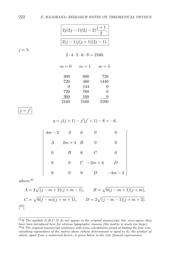
222 E. MAJORANA: RESEARCH NOTES ON THEORETICAL PHYSICS

2j(2j − 1)(2j − 2)j + 1

2,

2(j − 1)j(j + 1)(2j − 1).

j = 5:2 · 4 · 5 · 6 · 9 = 2160.

m = 0 m = 1 m = 5

360 600 720720 480 1440

0 144 0720 768 0360 168 0

2160 2160 2160

j = j′

η = j(j + 1) − j′(j′ + 1) − 6 = −6.

∣∣∣∣∣∣∣∣∣∣∣∣∣∣∣∣∣∣

4m − 2 A 0 0 0

A 2m + 4 B 0 0

0 B 6 C 0

0 0 C −2m + 4 D

0 0 0 D −4m − 2

∣∣∣∣∣∣∣∣∣∣∣∣∣∣∣∣∣∣

where:41

A = 2√

(j − m + 2)(j + m − 1), B =√

6(j − m + 1)(j + m),

C =√

6(j − m)(j + m + 1), D = 2√

(j − m − 1)(j + m + 2).

[42]

41@ The symbols A, B, C, D do not appear in the original manuscript, but, once again, theyhave been introduced here for obvious typographic reasons (the matrix is much too large).42@ The original manuscript continues with some calculations aimed at finding the four non-vanishing eigenvalues of the matrix above (whose determinant is equal to 0), the product ofwhich, apart from a numerical factor, is given below in the text (framed expressions).

ATOMIC PHYSICS 223

46j(j + 1)(2j − i)(2j + 3),

2j(2j − 1)(2j + 2)(2j + 3)

6.

j = 5:

m = 0 m = 1 m = 5

840 900 18030 30 810

600 486 135030 252 0

840 672 02340 2340 2340

3.16. RESONANCE BETWEEN A p (� = 1)ELECTRON AND AN ELECTRONWITH AZIMUTHAL QUANTUMNUMBER �′

Complex spectra are again considered, now evaluating resonance termsbetween electrons belonging to different shells.

Exchange energy:

K(n, 1,m�; n′, l′,m′�) =

∑bkGk,

Gk = er(4π)2∫ ∞

0

∫ ∞

0R(n, 1, r)R(n′, l′, r)R(n, 1, r′)R(n′, l′, r′)

× rkn

rk+1�

r2r′2dr dr′,

where:

224 E. MAJORANA: RESEARCH NOTES ON THEORETICAL PHYSICS

m� m′� b0 b1 b2 b3 b4

� = 1 �′ = 1 ±1 ±1 1 0 1/25 0 0±1 0 0 0 3/25 0 0±1 ∓1 0 0 6/25 0 0

0 0 1 0 4/25 0 0

� = 1 �′ = 2 ±1 ±2 0 2/5 0 3/245 0±1 ±1 0 1/5 0 9/245 0±1 0 0 1/15 0 18/245 0±1 ∓1 0 0 0 30/245 0±1 ∓2 0 0 0 90/245 0

0 ±2 0 0 0 15/245 00 ±1 0 1/5 0 24/245 00 0 0 4/15 0 27/245 0

Only the coefficients b�′−1 and b�′+1 are non vanishing.

3.16.1 Resonance Between A d Electron And Ap Shell I

`

m′s = 1/2

´ `

m′s = 1/2

´

m� ms m′� = 2 m′

� = 1 m′� = 0 m′

� = −1 m′� = −2

1 −1/2 0 0 0 0 00 −1/2 0 0 0 0 0

−1 −1/2 0 0 0 0 01 1/2 A B C D E R0 1/2 F G H G F R

−1 1/2 E D C B A R

S S S S S

where:43

43@ The symbols A, B, C, D, E, F, G, H, R, S do not appear in the original manuscript, buthave been introduced here for typographic reasons. Note that in the last row the author gavethe sum of all the terms in the corresponding column (for example, S = A + F + E, orS = B + G + D, etc.). He proceeded similarly with respect to the last column (for example,R = A + B + C + D + E, etc.).

ATOMIC PHYSICS 225

A =25G1 +

3245

G3, B =15G1 +

9245

G3,

C =115

G1 +18245

G3, D =30245

G3,

E =45245

G3, F =15245

G3,

G =15G1 +

24245

G3, H =415

G1 +27245

G3,

S =25G1 +

63245

G3, R =23G1 +

2449

G3.

3.16.2 Eigenfunctions Of d52, d3

2, p3

2And p1

2

ElectronsThe eigenfunctions are expressed by means of the notation (n′, �′,m′

j ,m′s).

We replace (n′, �′,m′�,m

′s) simply with (m′

�,m′s).

For d 52

:

j′ m′

5

2

5

2

„

2,1

2

«

5

2

3

2

r

4

5

„

1,1

2

«

+

r

1

5

„

2,−1

2

«

5

2

1

2

r

3

5

„

0,1

2

«

+

r

2

5

„

1,−1

2

«

5

2−1

2

r

2

5

„

−1,1

2

«

+

r

3

5

„

0,−1

2

«

5

2−3

2

r

1

5

„

−2,1

2

«

+

r

4

5

„

−1,−1

2

«

5

2−5

2

„

−2,−1

2

«

226 E. MAJORANA: RESEARCH NOTES ON THEORETICAL PHYSICS

For d 32

:

j′ m′

3

2

3

2

r

1

5

„

1,1

2

«

−r

4

5

„

2,−1

2

«

3

2

1

2

r

2

5

„

0,1

2

«

−r

3

5

„

1,−1

2

«

3

2−1

2

r

3

5

„

−1,1

2

«

−q

25

„

0,−1

2

«

3

2−3

2

r

4

5

„

−2,1

2

«

−r

1

5

„

−1,−1

2

«

For p 32

:

j m

3

2

3

2

„

1,1

2

«

3

2

1

2

r

2

3

„

0,1

2

«

+

r

1

3

„

1,−1

2

«

3

2−1

2

r

1

3

„

−1,1

2

«

+

r

2

3

„

0,−1

2

«

3

2−3

2

„

−1,−1

2

«

For p 12

:

j m

1

2

1

2

r

1

3

„

0,1

2

«

−r

2

3

„

1,−1

2

«

1

2−1

2

r

2

3

„

−1,1

2

«

−r

1

3

„

0,−1

2

«

ATOMIC PHYSICS 227

3.16.3 Resonance Between A d Electron And Ap Shell II

d 52

j m m′ = 5/2 m′ = 3/2 m′ = 1/2 m′ = −1/2 . . . . . .

p 32

3/2 3/2 A B C D3/2 1/2 E3/2 −1/2 F3/2 −3/2 0

S1

mean values T1

p 12

1/2 1/2 G1/2 −1/2 H

S2

mean values T2

S1

S2

Smean values T

where:44

A =25G1 +

3245

, B =425

G1 +36

1125G3, C = . . . ,

D = . . . , E =10245

G3, F =15245

G3,

G =5

245G3, H =

30245

G3,

S1 =25G1 +

28245

G3, T1 =110

G1 +7

245G3,

S2 =35245

G3, T2 =35490

G3,

S =25G1 +

63245

G3, T =115

G1 +21490

G3.

44@ See the previous footnote. Notice also that S = S1 + S2, and analogously for the Tterms.Here the manuscript is corrupted and we have represented by dots the expressions we cannoteasily interpret.

228 E. MAJORANA: RESEARCH NOTES ON THEORETICAL PHYSICS

d 32

j m m′ = 5/2 m′ = 3/2 m′ = 1/2 m′ = −1/2

p 32

3/2 3/2 A B C D3/2 1/23/2 −1/23/2 −3/2

S1

mean values T1

p 12

1/2 1/21/2 −1/2

S2

mean values T2

Smean values

where:45

A = . . . , B = . . . , C = . . . , D = . . . ,

S1 =115

G1 +63245

G3, T1 =160

G1 +63980

G3,

S2 =13G1, T2 =

16G1,

S =25G1 +

63245

G3.

Mean values:

d 52p 3

2:

115

G1 +21490

G3 +16

(15G1 −

21245

G3

)=

110

G1 +7

245G3,

d 52p 1

2:

115

G1 +21490

G3 −13

(15G1 −

21245

G3

)=

114

G3,

d 32p 3

2:

115

G1 +21490

G3 −14

(15G1 −

21245

G3

)=

160

G1 +63980

G3,

d 32p 1

2:

115

G1 +21490

G3 +12

(15G1 −

21245

G3

)=

16G1.

45@ See the previous footnote.

ATOMIC PHYSICS 229

If G1 = 1 and G3 =12:

d 52p 3

2: 0.0881 +

16· 0.1571 = 0.1143,

d 52p 1

2: 0.0881 − 1

3· 0.1571 = 0.0357,

d 32p 3

2: 0.0881 − 1

4· 0.1571 = 0.0488,

d 32p 1

2: 0.0881 +

12· 0.1571 = 0.1667.

3.17. MAGNETIC MOMENT ANDDIAMAGNETIC SUSCEPTIBILITYFOR A ONE-ELECTRON ATOM(RELATIVISTIC CALCULATION)

The following notes are aimed at evaluating the magnetic moment of anhydrogen-like atom by starting from the Dirac equation for an electronin an electromagnetic potential field (ϕ,C).

In the non-relativistic case:

σμ = − e2

6mc2

3a20

Z2.

[(W

c+

e

cϕ

)+ ρ1 σ ·

(p +

e

cC)

+ ρ3mc

]ψ = 0,

ϕ = +Ze

r.

A = (ψ1, ψ2), B = (ψ3, ψ4),

(W

c+

Ze2

rc+ mc

)A + σ

(p +

e

cC)

B = 0,

(W

c+

Ze2

rc− mc

)B − σ

(p +

e

cC)

A = 0.

230 E. MAJORANA: RESEARCH NOTES ON THEORETICAL PHYSICS

Cx = −12yH, Cy =

12xH, Cz = 0;

Hx = 0, Hy = 0, Hz = H.

W = −Ze2

r− ρ3mc2 − cρ1 σ · p − eH

rρ1(xσy − yσx).

∂W

∂H= −μz.

[W +

Ze2

r+ ρ3mc2 + cρ1σ · p +

e

2Hρ1(xσy − yσx)

]ψi = 0,

ψ = ψ0 + Hψ1 + H2ψ2 + . . . ,

W = W0 + HW1 + H2W2 + . . . .

[W0 +

Ze2

r+ ρ3mc2 + cρ1σ · p

]ψ0 = 0,

[W0 +

Ze2

r+ ρ3mc2 + cρ1σ · p

]ψ1 +

[W1 +

e

2ρ1(xσy − yσx)

]ψ0 = 0,

[W0 +

Ze2

r+ ρ3mc2 + cρ1σ · p

]ψ2

+[W1 +

e

2ρ1(xσy − yσx)

]ψ1 + W2ψ0 = 0.

W1 = −e

2

∫ψ0ρ1(xσy − yσx)ψ0dτ .

ATOMIC PHYSICS 231

W2 =e

2

∫ψ0ρ1(xσy − yσx)ψ1dτ − W1

∫ψ0ψ1dτ

= −∫

ψ0

[W1 +

e

2ρ1(xσy − yσx)

]ψ1dτ

= −∫

ψ1

[W1 +

e

2ρ1(xσy − yσx)

]ψ0dτ.

ψ0 = (A0, B0):

(W0 +

Ze2

r+ mc2

)A0 + cσ · pB0 = 0,

(W0 +

Ze2

r− mc2

)B0 − cσ · pA0 = 0.

A0 = f0Sm−1, B0 = g0S

m1 ,

(m = ±1/2, k = 1)

Smk = S

±l/21 .

(W0 +

Ze2

r+ mc2

)f0 + c

h

2πi

ddr

g0 = 0,

(W0 +

Ze2

r− mc2

)g0 − c

h

2πi

(ddr

+2r

)f0 = 0.

f0 =u0

r, g0 =

iv0

r:

(W0 + mc2 +

Ze2

r

)u0 + c

h

2π

(ddr

− 1r

)v0 = 0,

(W0 − mc2 +

Ze2

r

)v0 + c

h

2π

(ddr

+1r

)u0 = 0.

232 E. MAJORANA: RESEARCH NOTES ON THEORETICAL PHYSICS

p2 =W 2

c2− m2c2,

−W 20 + m2c4 =

4π2e4

h2c2m2c4Z2,

√−W 2

0 + m2c4 =2πc2

hcmcZ =

2πe2

hmZ,

α =2πe2

hc,

W0 = mc2√

1 − Z2α2, a0 =h2

4π2mc2.

v0 = r√

1−Z2α2e−Zr/a0 ,

u0 =Zα

1 +√

1 − Z2α2r√

1−Z2α2e−Zr/a0 .

(ddr

− 1r

)v0 = v0

(√1 − Z2α2

r− Z

a0− 1

r

)

= v0

(W − mc2

r mc2− Z

a0

),

and substituting in the equation above:

v0

(W − mc2

r mc2− Z

a0

)+

2π

hc

(W0 + mc2 +

Ze2

r

)u0 = 0,

u0 = −W0 − mc2 − r

a0mc2Z

r(W0 + mc2) + Ze2

hc

2πmc2v0

=mc2 − W0 +

mc2Z

a0r

Ze2 + (W0 + mc2)rh

2πmc2u0.

ATOMIC PHYSICS 233

3.18. THEORY OF INCOMPLETE P ′

TRIPLETS

On pages 61-68 and 90-116 of Quaderno 7, the author elaborated thetheory of incomplete P ′ triplets, as published by him in E. Majorana,Nuovo Cim. 8 (1931) 107. In the following, we reproduce only few topicsthat were not included in the published paper (which may be consultedfor further reference).

3.18.1 Spin-Orbit Couplings And Energy Levels

c s1 · �1 + c s2 · �2

�1 = 1 s1 = 1/2 j1 s1 · �1

3/2 1/21/2 −1

c =23δ, δ =

32c.

Interaction Diagonal terms ofterms s1 · �1 + s2 · �2

1D2 A + B/25 03P2

3P13P0 A − B/5 −1 −1/2 1/2

1S0 A + 2B/5 0

s · � = sx�x + sy�y + sz�z

=12

(sx + isy) (�x − ily) +12

(sx − isy) (�x + i�y) + σz�z.

The quantity � · s for � = 1, s = 1/2 is as follows:

[See the table on page 234.]

234 E. MAJORANA: RESEARCH NOTES ON THEORETICAL PHYSICS

For atoms with one p electron in the inner shells and one s in the outerone (like neon), denoting with I the exchange energy, we have:

[See the tables on page 235.]

For high Z and I = 1:

[See the figure on page 236.]

�z sz

jz

1 12

12

0 12

12

1 − 12

12

−1 12

− 12

0 − 12

− 12

−1 − 12

− 32

1 12

12

12

0 0 0 0 0

0 12

12

0 0√

22

0 0 0

1 − 12

12

0√

22

− 12

0 0 0

−1 12

− 12

0 0 0 − 12

√2

20

0 − 12

− 12

0 0 0√

22

0 0

−1 − 12

− 32

0 0 0 0 0 12

ATOMIC PHYSICS 235

m = 2

�z s1z s2

z 11

2

1

2

11

2

1

2−I +

1

2c

m = 1

�z s1z s2

z 01

2

1

21 − 1

2

1

21

1

2− 1

2

01

2

1

2−I c

√2

20

1 −1

2

1

2c

√2

2−1

2c −I

11

2−1

20 −I 1

2c

m = 0

�z s1z s2

z −11

2

1

20 − 1

2

1

20

1

2− 1

21 − 1

2− 1

2

−11

2

1

2−I − 1

2c

√2

2c 0

0 −1

2

1

2

√2

2c 0 −I 0

01

2−1

20 −I 0

√2

2c

1 −1

2−1

20 0

√2

2c −I − 1

2c

236 E. MAJORANA: RESEARCH NOTES ON THEORETICAL PHYSICS

ATOMIC PHYSICS 237

3.18.2 Spectral Lines For Mg And Zn[46]

Zn Mg(22′) 2086.72 2779.93(12′) 2070.11 2776.8021′ 2104.34 2783.0811′ 2087.27 2779.9301′ 2079.10 2778.3810′ 2096.88 2781.52

46The wavelengths of the following spectral lines are expressed in angstroms.

238 E. MAJORANA: RESEARCH NOTES ON THEORETICAL PHYSICS

3.18.3 Spectral Lines For Zn, Cd And Hg[47]

Zn Cd HgP ′

2 − P ′1 (399)

P ′1 − P ′

0 220 748 1938P ′

2 − P ′0 (619)

P2 − P1 389 1170 4534P1 − P0 189 544 1774P2 − P0 579 1714 6408

[48]

Zn Cd HgP ′

1 − P2 2104.34 47521 2329.27 42932 2002.7 49933P ′

1 − P1 2087.27 47910 2267.46 44102 1832.6 54567P ′

1 − P0 2079.10 48098 2239.85 44646 1774.9 56341P ′

0 − P1 2096.88 47690 2306.61 43354 1900.1 52629

47As above, the wavelengths of the following spectral lines are expressed in angstroms.48In the following table the author reported the wavelength (in angstroms) and the frequency(in cm−1) for the spectral lines in the first and the second column, respectively, for eachelement. As pointed out by the author himself, these values do not take into account thecorrection induced by propagation of light in air.

ATOMIC PHYSICS 239

3.19. HYPERFINE STRUCTURE:RELATIVISTIC RYDBERGCORRECTIONS

A relativistic formula for the Rydberg corrections of the hyperfine struc-tures was derived in the following calculations. Some particular cases,including s-orbit terms, were considered in detail. Probably, the presentcalculations were at the basis of what discussed in an appendix of E.Fermi and E. Segre, Mem. Accad. d’Italia 4 (1933) 131 on the sametopic, as acknowledged by the authors themselves.By using electronic units: γ =

√k2 − α2, α = Z/c.

μ0 = γ, α =√

k2 − γ2, μ0 + k = k + γ.

A = μ0 + k = k + γ, B = nr + γ, L =√

(nr + γ)2 + α2.

E = cB

L− c2,

E

c+ 2c = c

B

L+ c.

β =αc

L, αβ =

α2c

L.

dE

dnr= αc2 1

[(nr + γ)2 + α2]3/2.

a+μ0−1 =

α

c

11 − 2γ

.

β(μ0 + k) = αcA

L, −α

E

c= αc − αc

B

L.

b+μ0−1 = −A − 1

c

11 − 2γ

,

bμ0+1 =αc

L− 2αc

B

L(1 + 2γ)− αc

A(1 + 2γ)− αc

B

A L(1 + 2γ).

240 E. MAJORANA: RESEARCH NOTES ON THEORETICAL PHYSICS

2γC =(

A c + A cB

L+

α2c

L

)α

c

11 − 2γ

−(

αcA

L+ αc − αc

B

L

)A − 1

c(1 − 2γ)

−αA

L+ 2α

A B

L(1 + 2γ)+

α

1 + 2γ+ α

B

L(1 + 2γ)

=α

L

(AB

1 − 2γ+

α2

1 − 2γ− A2 − A

1 − 2γ+

AB − B

1 − 2γ

−A +2AB

1 + 2γ+

B

1 + 2γ

)+ α

(A

1 − 2γ− A − 1

1 − 2γ+

11 + 2γ

).

−C =α

√(nr + γ)2 + α2

12γ(4γ2 − 1)

·[4k(nr + γ) + 2

√(nr + γ)2 + α2

]

−dE

dε=

z2α

[(nr + γ)2 + α2]21

2γ(4γ2 − 1)

·[4k(nr + γ) + 2

√(nr + γ)2 + α2

]= −

∫uv

r2dr.

For Z → 0 (α2 → 0, γ = k, nr + γ = n):

−C =±α

2k (k − 1/2),

−dE

dε=

±Z2α

2n3k (k − 1/2).

In particular (2j + 1 = |2k|), for k = � + 1, j = � + 1/2:

−C =α

2(� + 1) (� + 1/2),

−dE

dε=

Z2α

2n3 (� + 1/2) (� + 1),

ATOMIC PHYSICS 241

while, for k = −�, j = � − 1/2:

−C =−α

2� (� + 1/2),

−dE

dε=

−Z2α

2n3� (� + 1/2).

The ratio R between the Rydberg corrections for the hyperfine structuresin the relativistic form and those in the classical (non-relativistic) formis then given by:

R =(2j + 1) (k − 1/2)

γ(4γ2 − 1)

(

2knr + γ

√(nr + γ)2 + α2

+ 1

)

.

For nr → ∞:

R =(j + 1/2)(4k2 − 1)

γ(4γ2 − 1).

For j = 1/2:

R =1

γ(4γ2 − 1)

[

2nr + γ

√(nr + γ)2 + α2

+ 1

]

,

and, for n = 1, 2, . . .:

1s : R =1

2γ2 − γ=

2γ + 1γ(4γ2 − 1)

,

2s : R =1 +

√2 + 2γ

γ(4γ2 − 1),

. . .

∞s : R =3

γ(4γ2 − 1).

242 E. MAJORANA: RESEARCH NOTES ON THEORETICAL PHYSICS

The corrections T on the absolute value of the hyperfine structures areinstead:

T = Rn3

[(nr + γ)2 + α2]3/2.

For the s terms we have nr = n − 1, γ2 + α2 = 1:

T = Rn3

[n2 − 2(n − 1)(1 − γ)]3/2.

In particular:

1s T =1

2γ2 − γ,

2s T =8[(2 + 2γ) +

√2 + 2γ]

γ(2γ − 1)(2γ + 1)(2 + 2γ)2,

. . .

8T1s

T2s=

(2γ + 1)(2 + 2γ)2

2 + 2γ +√

2 + 2γ=

(2γ + 1)(2 + 2γ)1 + 1/

√2 + 2γ

.

For γ = 0.74:

8T1s

T2s=

2.48 · 3.481 + 1/

√3.48

=8.631.536

= 5.62.

3.20. NON-RELATIVISTICAPPROXIMATION OF DIRACEQUATION FOR A TWO-PARTICLESYSTEM

After having obtained the usual non-relativistic decomposition of theDirac wavefunction (at a first as well as at a second approximation),the author considered a particular expression for of the electromagneticinteraction between a system of two identical charged particle (probablyelectrons in an atom). Then, he obtains the radial equations for theDirac components in a central field ϕ.

ATOMIC PHYSICS 243

3.20.1 Non-Relativistic Decomposition

α = ρ1σ, ψ = (A,B);

ρ1ψ = ρ1(A,B) = (B,A), ρ3ψ = ρ3(A,B) = (A,−B);

σψ = (σA,σB), ρ1σψ = (σB,σA);

ψαψ = AσB + BσA

(W

c+

e

cϕ

)ψ + ρ1

(σ,p +

e

cU)

ψ + ρ3 mc ψ = 0.

([W

c+

e

cϕ

]A,

[W

c+

e

cϕ

]B

)

+([

σ,p +e

cU]B,

[σ,p +

e

cU]A)

+ (mcA, −mcB) = 0.

(W

c+

e

cϕ

)A +

(σ,p +

e

cU)

B + mc A = 0,

(W

c+

e

cϕ

)B +

(σ,p +

e

cU)

A − mc B = 0.

For U = 0:(

W

c+

e

cϕ

)A + (σ,p) B + mc A = 0,

(W

c+

e

cϕ

)B + (σ,p)A − mc B = 0.

Since (σ,p) (σ,p) = p2:(

W

c+

e

cϕ

)B − 1

2mcp2 − mc B = 0,

W = mc2 − eϕ +1

2mp2.

244 E. MAJORANA: RESEARCH NOTES ON THEORETICAL PHYSICS

In a first approximation:

A = − 12mc

(σ,p) B,

while, in the second approximation:

A = − 12mc

(σ,p) B +W + eϕ

4m2c3(σ,p) B.

3.20.2 Electromagnetic Interaction BetweenTwo Charged Particles

By considering the total interaction:

e2

r12

(1 − (α,α′)

),

the magnetic interaction term is:

− e2

r12(α,α′) = − e2

r12ρ1ρ

′1 (σ,σ′).

The 4 components Aij of the wavefunction may be written as:

A11 A12 A21 A22

ψ1ψ2 ψ1ψ2 ψ3ψ4 ψ3ψ4

ψ′1ψ

′2 ψ′

3ψ′4 ψ′

1ψ′2 ψ′

3ψ′4

The complete expression for the energy is:

W = −e ϕ(q) − e ϕ(q′) − cρ1 (σ,p) − cρ′1(σ′ · p′)

−ρ3 mc2 − ρ′3 mc2 +e2

r12− e2

r12ρ1ρ

′1

(σ · σ′) .

In first approximation:

A12 = − 12mc

(σ,p) A22,

A21 = − 12mc

(σ′,p′)A22.

ATOMIC PHYSICS 245

3.20.3 Radial EquationsA = (ψ1, ψ2), B = (ψ1, ψ4):

(W

c+

e

cϕ

)A + (σ,p) B + mc A = 0,

(W

c+

e

cϕ

)B + (σ,p) A − mc B = 0.

By introducing the two-valued Pauli spherical function L correspondingto (�, j), and L1 = σzL corresponding to (�1, j) (with �1 = 2j − �):

B = g(r)L, A = f(r)σrL = f(r)L1

(it having been put L = σzL1).

(σ,p) A = (σ,p) f(r)σrL

= (σxpx + σypy + σzpz)f(r)(x

rσx +

y

rσy +

z

rσz

)L

= pxf(r)x

rL + pyf(r)

y

rL + prf(r)

z

rL

+i[pxf(r)

y

r− pyf(r)

x

r

]σzL

+i[pyf(r)

z

r− pzf(r)

y

r

]σxL

+i[pzf(r)

x

r− pxf(r)

z

r

]σyL.

pxf(r)x

rL =

x2

r2L prf(r) +

h

2πi

r2 − x2

r3f(r)L + f(r)

x

rpxL,

pyf(r)z

rσxL =

z

rσxL

y

rprf(r) − h

2πi

yr

r3f(r)σxL + f(r)

z

rσxpyL

=yz

r2σxL prf(r) − h

2πi

yr

r3f(r) σxL +

f(r)r

σx zpyL;

[pyf(r)

z

r− pzf(r)

y

r

]σxL = −f(r)

r(ypz − zpy) σxL.

(σ,p) A = L

{prf(r) +

z

r

h

2πif(r) − i

f(r)r

h

2π(σ, �)

},

(σ,p) A = L

{h

2π

∂f

∂r+

h

2πi

z

rf(r) +

h

2πi

f(r)r

(k − 1)}

f(r).

246 E. MAJORANA: RESEARCH NOTES ON THEORETICAL PHYSICS

(σ, �) ={

�−� − 1 = k − 1, (σ, �1) =

{−� − 2

� + 1 = −(k + 1).

(W + mc2 + eϕ

)f(r) + c

h

2πi

{ddr

− k − 1r

}g(r) = 0,

(W − mc2 + eϕ

)g(r) + c

h

2πi

{ddr

+k + 1

r

}f(r) = 0.

By setting r · g(r) = v, r · f(r) = i u:49

(W + mc2 + eϕ

)u − c

h

2π

(ddr

− k

r

)v = 0,

(W − mc2 + eϕ

)v + c

h

2π

(ddr

+k

r

)u = 0.

3.21. HYPERFINE STRUCTURES ANDMAGNETIC MOMENTS: FORMULAEAND TABLES

In the following the author reported some final formulae concerning hisstudies on hyperfine structures and the atomic magnetic moments (asin the previous Section, he set E = W − mc2, eϕ = −V ). Relatedcalculations are developed in the next Section.

(E − V + 2mc2) u − ch

2π

(ddr

− k

r

)v = 0,

(E − V ) v + ch

2π

(ddr

+k

r

)u = 0,

49In the original manuscript, the second equation in the following is written incorrectly as:

`

W − mc2 − eϕ´

v + ch

2π

„

d

dr+

k

r

«

u = 0.

ATOMIC PHYSICS 247

k =

⎧⎪⎪⎪⎪⎨

⎪⎪⎪⎪⎩

� + 1(

j = � +12

),

−�

(j = � − 1

2

),

k =(

j +12

)2

− �(� + 1), |k| = j +12,

k(k − 1) = �(� + 1).

Atomic magnetic moment:

μ0 =eh

4πmc, −M = j g(j) μ0 = −e

k

j + 1

∫r u v dr, (1)

μ0 g(j) = −k

j

e

j + 1

∫r u v dr. (1′)

Magnetic field at the origin:

j C = H =2k

j + 1e

∫u v

r2dr, (2)

C =2k

j(j + 1)e

∫u v

r2dr. (2′)

Nuclear magnetic moment:

Mn = i g(i)μ0

1840= i g(i) μ, μ =

eh

4πMnc=

μ0

1840. (2)

Hyperfine structure formula:

δW = −(Mn,H) = −(i, j) g(i) μ C

= −(i, j) g(i) μ2k

j(j + 1)e

∫u v

r2dr,

(3)

[50]

50@ In the following the author introduced the sum f = i + j.

248 E. MAJORANA: RESEARCH NOTES ON THEORETICAL PHYSICS

(i, j) =f(f + 1) − i(i + 1) − j(j + 1)

2.

——————–

In first approximation:

u =h

4πmc

(ddr

− k

r

)v,

∫ru v dr = −

(k +

12

)h

4πmc= −

(k +

12

)− μ0

e,

∫u v

r2dr = − (k − 1)

h

4πmc

1r3

= − (k − 1)1r3

μ0

e.

Atomic magnetic moment:

−M

μ0=

k(k + 1/2)j + 1

,

g(j) =k(k + 1/2)j(j + 1)

=

⎧⎪⎪⎪⎪⎨

⎪⎪⎪⎪⎩

2� + 22� + 1

(j = � +

12

),

2�

2� + 1

(j = � − 1

2

).

Magnetic field at the origin:

H = j C = −2k(k − 1)j + 1

μ01r3

= −2�(� + 1)j + 1

μ01r3

,

C = −2k(k − 1)j(j + 1)

μ01r3

= −2�(� + 1)j(j + 1)

μ01r3

.

Hyperfine structure formula:

δW =μ2

0

1840(i, j) g(i)

2k(k − 1)j(j + 1)

1r3

=μ2

0

1840(i, j) g(i)

2�(� + 1)j(j + 1)

1r3

.

For s-terms:∫

u v

r2dr = −2πψ2(0)

h

4πmc= −2πψ2(0)

μ0

e.

ATOMIC PHYSICS 249

H = j C = −8π

3ψ2(0) μ0,

C = −16π

3ψ2(0) μ0.

δW =μ2

0

1840(i, j) g(i)

16π

3ψ2(0) =

μ20

1840(2i + 1) g(i)

8π

3ψ2(0).

——————–

In first approximation, with a Coulomb field:

1r3

=Z3

a30

1n3 �(� + 1/2)(� + 1)

and, for s-terms,

ψ2(0) =Z3

a30

1πn3

.

2�(� + 1)j(j + 1)

1r3

s-terms:16π

3ψ2(0)

⎫⎪⎪⎪⎬

⎪⎪⎪⎭

=Z3

a30

4n3 j(j + 1)(2� + 1)

δW =μ2

0

1840(i, j) g(i)

Z3

a30

4n3 j(j + 1)(2� + 1)

(which holds also for s-terms).

μ20/a3 =

12

α2 Rh, α =2πe2

hc, α2R/c = 5.83 cm−1.

δW =2α2Rh1840

(i, j) g(i)Z3

n3 j(j + 1)(2� + 1),

δW

hc= δn = 0.00634 (i, j) g(i)

Z3

n3 j(j + 1)(2� + 1)cm−1.

The term δn1 corresponds to the particular case f = i + j, that is,cos i j = 1 and (i, j) = i j:

250 E. MAJORANA: RESEARCH NOTES ON THEORETICAL PHYSICS

δn1 = 0.00634Z3 i g(i)

n3 (j + 1)(2� + 1)cm−1.

——————–

a + b = c:

cos a b =(a, b)a b

,

(a, b) =c(c + 1) − a(a + 1) − b(b + 1)

2.

a b c (a, b) cos ca b

1/2 1/2 1 1/4 10 −3/4 −3

1 1/2 3/2 1/2 11/2 −1 −2

2 1/2 5/2 1 13/2 −3/2 −3/2

� 1/2 � + 1/2 �/2 1� − 1/2 −(� + 1)/2 −(� + 1)/2

a b c (a, b) cos ca b

1 1 2 1 11 −1 −10 −2 −2

3/2 1 5/2 3/2 13/2 −1 −7/31/2 −5/2 −5/3

2 1 3 2 12 −1 −1/21 −3 −3/2

3 1 4 3 13 −1 −1/32 −4 −4/3

� 1 � + 1 � 1� −1 −1/�

� − 1 −(� + 1) −(� + 1)/�

ATOMIC PHYSICS 251

a b c (a, b) cos ca b

3/2 3/2 3 9/4 12 −3/4 −1/31 −11/4 −11/90 −15/4 −5/3

2 3/2 7/2 3 15/2 −1/2 −1/63/2 −3 −11/2 −9/2 −3/2

� 3/2 � + 3/2 3�/2 1� + 1/2 �/2 − 3/2 1/3 − 1/�� − 1/2 −�/2 − 2 −1/3 − 4/3�� − 3/2 −3�/2 − 3/2 −1 − 1/�

3.22. HYPERFINE STRUCTURES ANDMAGNETIC MOMENTS:CALCULATIONS

Some calculations concerning atomic systems with magnetic moment arepresented in the following, by using similar notations as in the previousSection. The Dirac equation for the u and v wavefunctions underliessuch study. Explicit iterative formulae for the perturbative calculationof the wavefunctions are given, as well as the relevant self-consistentrelations (left unsolved).

3.22.1 First MethodOn using electronic units:51

α = Z/c, μ0 = 1/2c.

(E +

Z

r+ 2c2

)u − c

(ddr

− k

r

)v = 0,

(E +

Z

r

)v + c

(ddr

+k

r

)u = 0.

51@ In the original manuscript, an unidentified reference (see pages 15 and 25) appears here.

252 E. MAJORANA: RESEARCH NOTES ON THEORETICAL PHYSICS

(E′ +

Z

r+ 2c2

)y1 − c

(ddr

− k

r

)y2 = ε ry2,

(E′ +

Z

r

)y2 + c

(ddr

+k

r

)y1 = 0

for ε → 0.

y1 = P ′e−β′r, y2 = Q′e−β′r,

P ′ =∑

a′μrμ, Q′ =∑

b′μrμ,

a′μ = aμ + ε a∗μ, etc. 52

Remembering that α = Z/c:

(μ + k)a′μ + α b′μ = β′a′μ−1 −E′

cb′μ−1,

−α a′μ + (μ − k)b′μ =(

E′

c+ 2c

)a′μ−1 + β′b′μ−1 −

E

cb′μ−2.

Note that it is unnecessary to vary β.

(μ + k) a∗μ + α b∗μ = β a∗μ−1 −E

cb∗μ−1 + β∗aμ−1 −

E∗

cbμ−1,

−α a∗μ + (μ − k) b∗μ =(

E

c+ 2c

)a∗μ−1 + β b∗μ−1 +

E∗

caμ−1

+β∗ bμ−1 −1c

bμ−2.

[β (μ + k) − α

E

c

]a∗μ +

[α β +

E

c(μ − k)

]b∗μ

=(

β β∗ +E

c

E∗

c

)αμ−1 +

(−β

E∗

c+

E

cβ∗

)bμ−1 −

E

c

1c

bμ−2.

Let us set

ν = μ0 + nr

52@ That is: b′μ = bμ + ε b∗μ, β′ = β + ε β∗, E′ = E + ε E∗.

ATOMIC PHYSICS 253

and assume that

bν = 0 but aν �= 0 :

(b∗ν = 0)

[β (ν + k) − α

E

c

]a∗ν =

(β β∗ +

E

c

E∗

c

)aν−1

+(−β

E∗

c+

E

cβ∗

)bν−1 −

E

c

bν−2

c.

(1)

⎧⎪⎪⎪⎪⎪⎪⎪⎪⎨

⎪⎪⎪⎪⎪⎪⎪⎪⎩

(ν + k + 1) a∗ν+1 + α b∗ν+1 = β a∗ν + β∗ aν − E∗

cbν

−α a∗ν+1 + (ν + 1 − k) b∗ν+1 =(

E

c+ 2c

)a∗ν +

E∗

caν

+β∗ bν − 1c

bν−1

(2)

⎧⎪⎪⎪⎪⎪⎪⎪⎪⎨

⎪⎪⎪⎪⎪⎪⎪⎪⎩

(ν + k + 2) a∗ν+2 + α b∗ν+2 = β a∗ν+1 −E

cb∗ν+1

−α a∗ν+2 + (ν + 2 − k) b∗ν+2 =(

E

c+ 2c

)a∗ν+1

+β b∗ν+1 −1c

bν

(3)

β a∗ν+2 −E

cb∗ν+2 = 0. (4)

We can set β∗ = 0 or, rather:

β∗ = βE∗

E.

254 E. MAJORANA: RESEARCH NOTES ON THEORETICAL PHYSICS

It follows that:

β β∗ +E

c

E∗

c=

E∗

E

(β2 +

E2

c2

)= −2E∗,

−βE∗

c+

E

cβ∗ = 0,

β∗aν − E∗

cbν = 0,

E∗

caν + β∗bν =

E∗

E

(E

caν + β bν

)= −2c

E∗

Eaν .

[β (ν + k) − α

E

c

]a∗ν = −2E∗aν−1 −

E

c2bν−2, (1′)

⎧⎪⎪⎨

⎪⎪⎩

(ν + k + i) a∗ν+1 + α b∗ν+1 = β a∗ν

−α a∗ν+1 + (ν + 1 − k) b∗ν+1 =(

E

c+ 2c

)a∗ν − 2c

E∗

Eaν − 1

cbν−1

(2′)

Equations (1′), (2′), (3) and (4) are six homogeneous equations in a∗ν ,a∗ν+1, b∗ν+1, a∗ν+2, b∗ν+2 and −1.

3.22.2 Second Method

⎧⎪⎪⎪⎪⎨

⎪⎪⎪⎪⎩

(E′ +

Z

r+ 2c2

)y1 − c

(ddr

− k

r

)y2 = ε ry2,

(E′ +

Z

r

)y2 + c

(ddr

+k

r

)y2 = ε ry1.

E∗ = Z

∫r u v dr.

ATOMIC PHYSICS 255

With the previous notations:

⎧⎪⎪⎪⎪⎪⎪⎪⎪⎪⎪⎪⎪⎪⎪⎨

⎪⎪⎪⎪⎪⎪⎪⎪⎪⎪⎪⎪⎪⎪⎩

(μ + k) a∗μ + α b∗μ = β a∗μ−1 −E

cb∗μ−1 + β∗ aμ−1

−E∗

cbμ−1 +

1c

aμ−2,

−α a∗μ + (μ − k) b∗μ =(

E

c+ 2c

)a∗μ−1 + β b∗μ−1 +

E∗

caμ−1

+β∗bμ−1 −1c

bμ−2.

ν = μ0 + νr.

bν = 0, aν �= 0.

Note that is is unnecessary to vary β.

[β (ν + k) − α

E

c

]aν =

(β β∗ +

E

c

E∗

c

)aν−1 −

(β

E∗

c

−E

cβ∗

)bν−1 +

β

caν−2 −

E

c2bν−2

(1)

(b∗ν = 0).

β a∗ν+2 −E

cb∗ν+2 = 0. (4)

⎧⎪⎪⎪⎨

⎪⎪⎪⎩

(ν + k + 2) a∗ν+2 + α b∗ν+2 = β a∗ν+1 −E

cb∗ν+1 +

1c

aν ,

−α a∗ν+2 + (ν + 2 − k) b∗ν+2 =(

E

c+ 2c

)a∗ν+1 + β b∗ν+1 −

1c

bν .

(3)

Note that a∗ν+2/b∗ν+2 is different from what obtained by Eq. (4), so thata∗ν+2 = b∗ν+2 = 0:

⎧⎪⎨

⎪⎩

a∗ν+2 = 0, b∗ν+2 = 0,

β a∗ν+1 −E

cb∗ν+1 +

1c

aν = 0.

256 E. MAJORANA: RESEARCH NOTES ON THEORETICAL PHYSICS

⎧⎪⎪⎪⎪⎪⎪⎪⎪⎨

⎪⎪⎪⎪⎪⎪⎪⎪⎩

(ν + k + 1) a∗ν+1 + α b∗ν+1 = β a∗ν + β∗ aν − E∗

cbν +

1c

aν−1,

−α a∗ν+1 + (ν + 1 − k) b∗ν+1 =(

E

c+ 2c

)a∗ν +

E∗

caν

+β∗ bν − 1c

bν−1.

(2)

[See the equations on pages 257 and 258.]53

a11 0 0 0 0 a16

−β a22 α 0 0 0

0 0 0 β −E

c0

a41 −α a43 0 0 a46

0 −βE

ca34 α 0

0 a62 −β −α a65 a66

= 0.

For a suitable value of β∗, from (3) and (4) we get:

a∗ν+1 = 0, b∗ν+1 =aν

E,

⎧⎪⎪⎪⎨

⎪⎪⎪⎩

α

Eaν = β a∗ν + β∗ aν − E∗

cbν +

1c

aν−1,

ν + 1 − k

Eaν =

(E

c+ 2c

)a∗ν +

E∗

caν + β∗bν − 1

cbν−1.

(2′)

Equations (1) and (2′) are homogeneous equations in a∗ν , β∗ and 1, sothat:

[See equation on page 259.]

53Note that the second determinant differs from the first one with respect the ordering ofthe rows (1,2,3,4,5,6 in the first, and 1,2,6,3,4,5 in the second matrix), as pointed out by theauthor himself in the original manuscript.

ATOMIC PHYSICS 257

β(ν

+k)−

αE c

00

00

−2E

∗ aν−

1−

E c2b ν

−2

−β

(ν+

k+

1)α

00

0

−(

E c+

2c)

−α

ν+

1−

k0

0−

2cE

∗

Ea

ν−

1 2b ν

−1

0−

βE c

ν+

k+

2α

0

0−(

E c+

2c)

−β

−α

ν+

2−

k−

1 cb ν

00

0β

−E c

0

=0

258 E. MAJORANA: RESEARCH NOTES ON THEORETICAL PHYSICS

β(ν

+k)−

αE c

00

00

−2E

∗ aν−

1−

E c2b ν

−2

−β

(ν+

k+

1)α

00

0

00

0β

−E c

0

−(

E c+

2c)

−α

ν+

1−

k0

0−

2cE

∗

Ea

ν−

1 2b ν

−1

0−

βE c

ν+

k+

2α

0

0−(

E c+

2c)

−β

−α

ν+

2−

k−

1 cb ν

=0

ATOMIC PHYSICS 259

βa

ν−

E∗ cb ν

+1 ca

ν−

1−

α Eα

ν

(E c

+2c)

b νE

∗ ca

ν−

1 cb ν

−1−

ν+

1−

k

Eα

ν

β(ν

+k)−

αE c

−(

βa

ν−

1+

E cb ν

−1

)−

E∗ c

(E c

aν−

1−

βb ν

−1

)−

β ca

ν−

2+

E c2b ν

−2

=0

4

MOLECULAR PHYSICS

4.1. THE HELIUM MOLECULE

4.1.1 The Equation For σ-electrons In EllipticCoordinates

We assume the nuclei to be fixed at a distance r one from the other(in electronic units); the nuclei are supposed to have positive charges,of magnitude Z ≤ 2, taking approximatively into account the screeningaction of the other electrons.

∇2 ψ + 2(

E +Z

r1+

Z

r2

)ψ = 0.

By measuring the energy (denoted with W ) in Rh we have W = 2E,from which:

∇2 ψ + Wψ + 2Z

(1r1

+1r2

)ψ = 0.

Putting:

u =r1 + r2

2, v =

r1 − r2

2,

r1 = u + v, r2 = u − v,

r21 = u2 + 2uv + v2, r2

2 = u2 − 2uv + v2, r1r2 = u2 − v2,

we have

∇2 ψ =∂2ψ

∂u2|∇ u|2 +

∂2ψ

∂v2|∇ v|2 +

∂ψ

∂u∇ ·u +

∂ψ

∂v∇ · v,

261

262 E. MAJORANA: RESEARCH NOTES ON THEORETICAL PHYSICS

and, since

|∇ u|2 =1 + cos(r1, r2)

2=

12

+r21 + r2

2 − 44r1r2

=12

+u2 + v2 − 22(u2 − v2)

=u2 − 1u2 − v2

,

|∇ v|2 =12− u2 + v2 − 2

2(u2 − v2)=

1 − v2

u2 − v2,

∇2 u =1r1

+1r2

=1

u + v+

1u − v

=2u

u2 − v2,

∇2 v =1r1

− 1r2

=1

u + v− 1

u − v= − 2v

u2 − v2,

it follows that

∇2 ψ =u2 − 1u2 − v2

∂2ψ

∂u2+

1 − v2

u2 − v2

∂2ψ

∂v2+

2u

u2 − v2

∂ψ

∂u− 2v

u2 − v2

∂ψ

∂v;

u2 − 1u2 − v2

∂2ψ

∂u2+

1 − v2

u2 − v2

∂2ψ

∂v2+

2u

u2 − v2

∂u

∂u− 2v

u2 − v2

∂ψ

∂v

+Wψ +2Z1

u + vψ +

2Z2

u − vψ = 0,

where, for the sake of generality, we have distinguished Z1 from Z2 (whilewe take the half-distance between the nuclei equal to 1). On multiplyingthe previous equation by (u2 − v2):

(u2 − 1)∂2ψ

∂u2+ 2u

∂ψ

∂u+ 2u(Z1 + Z2)ψ + (1 − v2)

∂2ψ

∂v2− 2v

∂ψ

∂v−2v(Z1 − Z2)ψ + u2Wψ − v2Wψ = 0. (1)

By settingψ = P1(u)P2(v),

and again Z1 = Z2 = Z, we have the following separated equations:

(u2 − 1)P ′′1 + 2uP ′

1 + 4uZP1 + u2WP1 − λP1 = 0, (2)(1 − v2)P ′′

2 − 2vP ′2 − v2WP2 + λP2 = 0. (3)

These equations have to be solved together in order to determine Wand λ. It is useful to deduce firstly a relation between W and λ fromthe second equation, which does not depend on Z (but depends on thedistance between the nuclei, which we have definitively chosen to be

MOLECULAR PHYSICS 263

equal to 2; with a similarity transformation we can always turn backto this case). Such a relation between W and λ depends only on theazimuthal quantum number, related to P2, and not on the radial one,corresponding to P1.

4.1.2 Evaluation Of P2 For s-electrons: RelationBetween W And λ

The quantity P2 does not change sign if we replace v with −v; v variesbetween −1 and 1; singular points are at v = −1 and v = 1. Let us setP2(−1) = 1, so that P ′

2(−1) is determined:

2P ′2(−1)W + λ = 0,

P ′2(−1) =

W − λ

2.

Quantity λ results as determined as the smallest value for which P ′2(0) =

0. In Eq. (2) we put, for the moment,

v = x − 1 = −1 + x, x = v + 1;

it follows:

(2x − x2)P ′′2 + (2 − 2x)P ′

2 − (1 − x)2WP2 + λP2 = 0;

and, setting:

P2 = 1 +W − λ

2x + bx2 + cx3 + . . . ,

P ′2 =

W − λ

2+ 2bx + 3cx2 + . . . ,

P ′′2 = 2b + 6cx + . . . ,

after some algebra1

b =(W − λ)2

16− W + λ

8,

c =b

3+

W − λ

18b +

W

18− W (W − λ)

18.

1@ In the original manuscript some scratch calculations are reported, leading to the follow-ing expressions for b and c (obtained by substituting the expansions for P2, P ′

2, P ′′2 into the

differential equation for P2 written above).

264 E. MAJORANA: RESEARCH NOTES ON THEORETICAL PHYSICS

P2 = 1 +W − λ

2x +

[(W − λ)2

16− W + λ

8

]x2 + cx3 + . . .

W = −1

λ = −0.3 λ = −0.4 λ = 0.348

v P2 −P ′2 P ′′

2 P2 −P ′2 P ′′

2 P2 −P ′2 P ′′

2

−1 1.000 0.350 0.396 1.000 0.300 0.395 1.000 0.326

−0.9 967 313 0.365 972 261 0.379 0.969

−0.8 937 277 0.346 948 224 0.364 0.942

−0.7 911 243 0.33 927 188 0.35 0.919

−0.6 888 211 0.31 910 153 0.34 0.899

−0.5 868 181 0.30 896 119 0.34 0.882

−0.4 852 151 0.29 886 085 0.33 0.868

−0.3 838 123 879 051 0.858

−0.2 0.850

−0.1 0.846

0 0.845

[2]

2@ The table reported in the original manuscript contains slightly different numerical valueswith respect to those one can evaluate from the formulae given by the author, namely:

W = −1

λ = −0.3 λ = −0.4 λ = 0.348

v P2 −P ′2 P ′′

2 P2 −P ′2 P ′′

2 P2 −P ′2 P ′′

2

−1 1.000 0.350 0.386 1.000 0.300 0.395 1.000 0.326

−0.9 0.967 0.313 0.368 0.972 0.261 0.377 0.969

−0.8 0.937 0.277 0.341 0.948 0.226 0.359 0.942

−0.7 0.911 0.244 0.32 0.927 0.189 0.34 0.919

−0.6 0.888 0.213 0.30 0.910 0.156 0.32 0.899

−0.5 0.869 0.185 0.27 0.896 0.125 0.31 0.881

−0.4 0.851 0.159 0.25 0.885 0.095 0.29 0.867

−0.3 0.837 0.135 0.877 0.067 0.856

−0.2 0.847

−0.1 0.840

0 0.835

Probably, the numerical values for the second derivative of P ′′2 were deduced in some manner

from the following formula (which appears in the manuscript):

P ′′2 =

2vP ′2 − (v2 + λ)P2

1 − v2.

MOLECULAR PHYSICS 265

Let us now set:

P2 = eR

zdv,

P ′2 = z e

R

zdv,

P ′′2 = (z′ + z2) e

R

zdv;

(1 − v2)z′ + (1 − v2)z2 − 2vz + λ − v2W = 0. (4)

By solving Eq. (4) with respect to z′:

z′ =2v

1 − v2z − λ − v2W

1 − v2− z2. (5)

λ and z are infinitesimals with W ; we will put:

z = z1 + z2 + z3 + . . . , λ = λ1 + λ2 + . . . ,

where z1 stands for a first-order infinitesimal, z2 for a second-order in-finitesimal, etc. We will have:

z′1 =2v

1 − v2z1 −

λ1 − v2W

1 − v2, (6)

from which, by imposing regularity conditions on the boundaries, 3

z1 = − 11 − v2

∫ v

−1(λ1 − v2W )dv

= − 11 − v

(λ1 −

13W +

13Wv − 1

3Wv2

).

We set:

q1 = z1 = −13Wv, (7)

�1 = λ1 =13W. (8)

When determining z2, etc., we will set:

q1 = z1, q2 = z1 + z2, q3 = z1 + z2 + z3, . . .

�1 = λ1, �2 = λ1 + λ2, �3 = λ1 + λ2 + λ3, . . .

3@ In the original manuscript the upper limit of the following integrals is not explicitlyindicated.

266 E. MAJORANA: RESEARCH NOTES ON THEORETICAL PHYSICS

In general we will have:

q′n+1 =2v

1 − v2qn+1 −

�n+1 − v2W

1 − v2− q2

n.

From it:

qn+1 =1

1 − v2

∫ v

−1

[v2W − �n+1 − (1 − v2) q2

n

]dv

=1

1 − v2

[13v3W +

13W − v �n+1 − �n+1 −

∫ v

−1(1 − v2) q2

n dv

]

=13

v2W − vW + W − 3�n+1

1 − v− 1

1 − v2

∫ v

−1(1 − v2) q2

n dv

= −13Wv +

11 − v

(−�n+1 +

13W − 1

1 + v

∫ v

−1(1 − v2) q2

n dv

),

and, by imposing the regularity at the point v = 1, it must be:

�n+1 =13W − 1

2

∫ 1

−1(1 − v2) q2

n dv. (9)

By substituting Eq. (9) into previous equation:

qn+1 = −13Wv +

11 − v

(12

∫ 1

−1(1 − v2) q2

n dv

− 11 + v

∫ v

−1(1 − v2) q2

n dv

), (10)

or, more easily,

qn+1 = −13Wv +

11 − v2

(12v

∫ 1

−1(1 − v2) q2 dv

−∫ v

0(1 − v2) q2

n dv

). (10′)

By taking into account that qn+1(v) = −qn+1(−v), we also have:

�n+1 = W − 2qn+1(−1) = W + 2qn+1(1), (11)

which can replace Eq. (9). Let us now evaluate q2; since q1 = −13Wv,

by substitution into Eq. (9′):

MOLECULAR PHYSICS 267

q2 = −13Wv +

11 − v2

[12v

∫ 1

−1(1 − v2)

(−1

3Wv

)2

dv

−∫ v

0(1 − v2)

(−1

3Wv

)2

dv

]

,

that is:

q2 = −13vW +

W 2

91

(1 − v2)

(215

v − 13v3 +

15v5

),

or, more simply:

q2 = −13vW −

(145

v3 − 2135

v

)W 2, (12)

l2 =13W − 2

135W 2.

Recalling that

z = z1 + z2 + z3 + . . . ,

λ = λ1 + λ2 + λ3 + . . . ,

qn = z1 + z2 + . . . + zn,

�n = λ1 + λ2 + . . . + λn,

and that zn and λn are infinitesimals of order n, with this procedure wecan obtain any term in the series expansion of z and λ with increasingpowers of W :

z = −13vW −

(145

v3 − 2135

v

)W 2 + . . . , (13)

λ =13W − 2

135W 2 + . . . . (14)

From z we can then obtain P2:

P2 = eR

zdv,

by choosing a suitable normalization, in such a way that P2(−1) =P2(1) = 1:

P2 = e16(1−v2)W− 1

540(1−4v2+3v4)W 2+... , (15)

P2(0) = e16W− 1

540W 2+... .

——————–

268 E. MAJORANA: RESEARCH NOTES ON THEORETICAL PHYSICS

The expansions (12), (13) and (15) cannot be used for large values of W .Then, we now consider asymptotic expansions with decreasing powersof W for W tending to the (negative) infinity. We will set:

z = y1 + y2 + y3 + . . . ,

λ = m1 + m2 + . . . ,

pn = y1 + . . . + yn,

Ln = m1 + . . . + mn,

where we always assume that mn+1/mn or yn+1/yn are infinitesimals forW → −∞ and consider only infinities of higher order. By substitutioninto Eq. (5):

y21 = −m1 − v2W

1 − v2, (16)

so that, by requiring regularity in the singular points,

L1 = m1 = W, (17)p1 = y1 = ±

√−W.

Since p1(v) = p1(−v) (and∫ 0−1 p1(v)dv is certainly negative) and p1 has

the same sign as v,

p1 = y1 = −√−W, v < 0;

p1 = y1 =√−W, v > 0.

(18)

Note that the discontinuity at the point 0 results in a divergence for z′

in Eq. (5), which cannot be neglected; however, by replacing the jumpwith a suitable junction line in the interval −ε, +ε, |z′| will be of theorder of

√−W/ε, while the other infinities are of the same order of W .

Then we can neglect z′ provided that:

ε√−W � 1,

and since W tends to the infinity, we may take the limit ε = 0.For the successive approximations we have to consider:

p′n =2v

1 − v2pn − Ln+1 − v2W

1 − v2− p2

n+1, (19)

and, imposing the regularity conditions,

Ln+1 = W − 2pn(−1) = W + 2pn(1), (20)

MOLECULAR PHYSICS 269

one gets

pn+1 = −√

−Ln+1 − v2W

1 − v2+

2v

1 − v2pn − p′n (v < 0), (21)

pn+1 =

√

−Ln+1 − v2W

1 − v2+

2v

1 − v2pn − p′n (v > 0). (22)

The asymptotic expansions of z do not yield a continuous curve andcannot be used in any interval around v = 0 whose extension is of theorder of

√−W . We will find later an appropriate approximation formula

for z.We now focus directly on the asymptotic expansion of λ as a functionof W .By integrating Eq. (2) from −1 to 0 we obtain:

λ = W

∫ 0

−1v2P2 dv

∫ 0

−1P2 dv

. (23)

For W → −∞ it suffices to integrate over a very small interval, startingat −1 for any order of approximation; this would be an indication of thefact that the asymptotic expansion is never convergent.By setting

x = 1 + v, v = x − 1,

Equation (2) becomes:

(2x − x2)P ′′2 + (2 − 2x)P ′

2 − (1 − x)2 WP2 + λP2 = 0, (24)

and, putting

P2 = Re−√−Wx,

P ′2 = (R′ − R

√−W )e−

√−Wx,

P ′′2 = (R′′ − 2R′√−W − RW )e−

√−Wx,

it follows:

(2x − x2)R′′ − [(2x − x2)2√−W − (2 − 2x)]R′ − (2x − x2)RW

−(1 − x)2RW − 2R(1 − x)√−W + λR = 0,

270 E. MAJORANA: RESEARCH NOTES ON THEORETICAL PHYSICS

that is:

(2x − x2)R′′ − 2[(2x − x2) −√

W − (1 − x)]R′

−[W − λ + 2(1 − x)√−W ]R = 0.

For x = 0 we will take R = 1. It follows:

2R′(0) = W − λ + 2√−W,

where from:

R = 1 +W − λ + 2

√−W

2x + bx2 + . . . ,

R′ =W − λ + 2

√−W

2+ 2bx + . . . ,

R′′ = 2b + . . . .

By substitution into the above equation, from the vanishing of first-orderterms, one has

4b − 2(W − λ − 2√−W )

√−W − (W − λ − 2

√−W ) + 2

√−W = 0,

where from:

b =(W − λ − 2

√−W − 1)

2

√−W +

W − lλ − 2√−W

4.

On the other hand, asymptotically we have:

λ = W − W

∫ ∞

0(2x − x2)P2dx∫ ∞

0P2dx

,

and, since

P2 = (1 + ax + bx2 + . . .) e−√−Wx,

(2x − x2)P2 = [2x + (2a − 1)x2 + (2b − a)x3 + . . .] e−√−Wx,

MOLECULAR PHYSICS 271

we deduce:

λ = W − W

2−W

+2a − 1

(−W )32

+2b − a

W 2

1√−W

+a

−W+

b

(−W )32

+ . . .

,

λ = W + 2√−W

1 +2a − 12√−W

+2b − a

−W − 2

1 +a√−W

+b

−W

= W + 2√−W − 1 + . . . .

Summing up, for the moment we know the behavior of the functionλ = λ(W ) for small and large values of W :

W → 0, λ =13W − 2

135W 2 + . . . ,

W → −∞, λ = W + 2W 2 +√−W − 1 + . . . .

(25)

Let us put againP2 = e

R v−1 rdv;

it follows:

z′ =2v

1 − v2z − λ − v2W

1 − v2− r2. (5)

As an approximate solution, we take:

z = a arctan b v. (26)

Substituting it into Eq. (5):

ab

1 + b2v2=

2va

1 − v2arctan b v − λ − v2W

1 − v2− u2 arctan2 b v + . . . . (27)

We require that this equation be satisfied for v = 0; it follows:

ab = −λ. (28)

Regularity conditions for v = 1 impose:

2a arctan b = λ − W. (29)

272 E. MAJORANA: RESEARCH NOTES ON THEORETICAL PHYSICS

We also require that the equation be satisfied for v = 1, since:

limv→1

2av arctan b v − λ + v2W

1 − v2= −W − a arctan b − ab

1 + b2.

It follows:

W + a arctan b +2ab

1 + b2+ a2 arctan2 b = 0. (30)

From Eqs. (28), (29), (30) we can determine a, b and λ. We can thenconsider the following equations:

W +(

λ − W

2

)2

+λ − W

2− 2λ

1 + b2= 0, (31)

b = tan(

bW − λ

2λ

)= tan

⎛

⎜⎝b

1 − λ

W

2λ

W

⎞

⎟⎠ , (32)

a = −λ

b. (33)

By taking a series expansion, for small W we have:

λ =13W + KW 2 + . . . ,

λ

W=

13

+ KW + . . . .

Equation (32) becomes:

b = tan

⎛

⎜⎝b

23− KW + . . .

23

+ 2KW + . . .

⎞

⎟⎠ = tan

(b − 9

2bKW + . . .

).

On the other hand:(

b − 92bKW

)= arctan b = b − 1

3b3 + . . . ,

from which:

−92KbW = −1

3b3 + . . . ,

b2 =272

KW + . . . .

MOLECULAR PHYSICS 273

Substituting it into Eq. (31):

1 +19W − 1

3+

12KW − 2

3− 2KW + 9KW + . . . = 0,

from which:

19

+12K − 2K + 9K = 0,

19

+152

K = 0,

K = − 2135

,

λ =13W − 2

135W 2 + . . . ,

which agrees with Eq. (25). We have thus an exact result holding infirst and second approximation:

b2 = −15W + . . . . (34)

For the asymptotic expansion (W → −∞), we set:

λ = W + 2√−W + α + . . . .

By substituting it into Eq. (31), noting that b is an infinite of order 1/2and equating to zero higher-order infinities, we have:

α√−W +

√−W = 0,

from which α = −1 and:

λ = W + 2√−W − 1 + . . . ,

which again agrees with Eq. (25). We can likely presume that forarbitrary W a very good approximation for λ = λ(W ) is obtained.

[4]−W −λ b

0 0 0

1 +0.348 0.47

2 +0.731 0.72

3 1.151 0.94

4

4@ It is not very clear how the author obtained the values reported in the following table.Probably, for a given value of W , λ was obtained from the approximate Eq. (25) for W → 0(in this case, for −W = 2, 3 we would have −λ = 0.726, 1.133), while b is deduced from Eq.(31).

274 E. MAJORANA: RESEARCH NOTES ON THEORETICAL PHYSICS

[5]

W = −2

λ = −0.72 λ = −0.74 λ = 0.73

v P2 −P ′2 P ′′

2 P2 −P ′2 P ′′

2 P2 −P ′2 P ′′

2

−1 1.000 0.640 0.885 1.000 0.630 0.883 1.000 635

−0.95 969.1 596.8 845 969.6 586.8 844 969 592

−0.9 940.3 555.5 808 941.3 545.5 808 941 550

−0.85

−0.8 888.7 478.0 741 890.7 468.0 744 890 473

−0.7 844.5 406.9 686 847.5 396.5 690 846 402

−0.6 807.2 340.5 638 811.2 329.8 644 809 335

−0.5 776 279 599 781 267.5 606 778.5 273

−0.4 751 221 568 757 208.5 577 754 215

−0.3 732 165 543 739 152 555 735.5 158

−0.2 718 112 525 726 97 540 722 105

−0.1 709 60 513 719 44 532 714 52

0 706 9 508 717 −9 531 711.5 0

W = −3

λ = −1.14 λ = −1.16 λ = 1.143

v P2 −P ′2 P ′′

2 P2 −P ′2 P ′′

2 P2 −P ′2 P ′′

2

−1 1.000 0.930 1.467 1.000 0.920 1.463 1.000 0.928

−0.95 955.3 858.9 1.379 955.8 849.1 1.377 955 857

−0.9 914.1 792.0 1.297 915.0 782.3 1.295 914 790

−0.85 876.1 729.1 1.223 877.5 719.5 1.222 876 728

−0.8 841.1 669.7 1.154 843.0 660.1 1.154 841 668

−0.7 780 561 1.032 783 551 1.033 780 559

−0.6 729 463 936 733 453 940 730 461

−0.5 687 373 855 692 363 862 688 371

−0.4 654 291 791 660 280 801 655 289

−0.3 629 214 743 636 202 756 630 212

−0.2 611 141 708 620 128 725 612 139

−0.1 600 71 687 611 56 708 602 69

0 597 3 680 609 −15 706 599 0

5@ The following two tables seem the continuation of the table appearing at page 264, but itis not clear how the author obtained the numerical values reported here. Note that, as above,in some places the author omits the notation “0.” in the reported numbers.Probably, the numerical values for the second derivative of P ′′

2 were deduced in some mannerfrom the following formula (which appears in the manuscript):

P ′′2 =

2vP ′2 − (2v2 + λ)P2

1 − v2,

for W = −2, and

P ′′2 =

2vP ′2 − (3v2 + λ)P2

1 − v2

for W = −3.

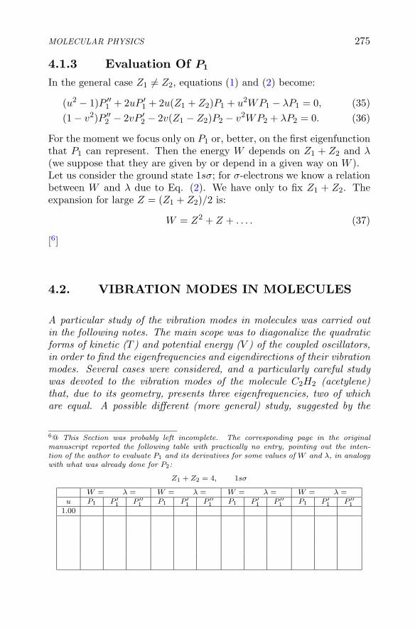
MOLECULAR PHYSICS 275

4.1.3 Evaluation Of P1

In the general case Z1 �= Z2, equations (1) and (2) become:

(u2 − 1)P ′′1 + 2uP ′

1 + 2u(Z1 + Z2)P1 + u2WP1 − λP1 = 0, (35)(1 − v2)P ′′

2 − 2vP ′2 − 2v(Z1 − Z2)P2 − v2WP2 + λP2 = 0. (36)

For the moment we focus only on P1 or, better, on the first eigenfunctionthat P1 can represent. Then the energy W depends on Z1 + Z2 and λ(we suppose that they are given by or depend in a given way on W ).Let us consider the ground state 1sσ; for σ-electrons we know a relationbetween W and λ due to Eq. (2). We have only to fix Z1 + Z2. Theexpansion for large Z = (Z1 + Z2)/2 is:

W = Z2 + Z + . . . . (37)

[6]

4.2. VIBRATION MODES IN MOLECULES

A particular study of the vibration modes in molecules was carried outin the following notes. The main scope was to diagonalize the quadraticforms of kinetic (T ) and potential energy (V ) of the coupled oscillators,in order to find the eigenfrequencies and eigendirections of their vibrationmodes. Several cases were considered, and a particularly careful studywas devoted to the vibration modes of the molecule C2H2 (acetylene)that, due to its geometry, presents three eigenfrequencies, two of whichare equal. A possible different (more general) study, suggested by the

6@ This Section was probably left incomplete. The corresponding page in the originalmanuscript reported the following table with practically no entry, pointing out the inten-tion of the author to evaluate P1 and its derivatives for some values of W and λ, in analogywith what was already done for P2:

Z1 + Z2 = 4, 1sσ

W = λ = W = λ = W = λ = W = λ =u P1 P ′

1 P ′′1 P1 P ′

1 P ′′1 P1 P ′

1 P ′′1 P1 P ′

1 P ′′1

1.00

276 E. MAJORANA: RESEARCH NOTES ON THEORETICAL PHYSICS

just considered molecule of acetylene, was envisaged at the end of thisSection.

T =12

∑x2

i , V =12

∑(xi − xi−1)2;

∂T

∂xi= xi,

∂V

∂xi= xi − xi−1 − xi+1 + xi = 2xi − xi+1 − xi−1.

The equation of motion is then:

xi = xi+1 − 2xi + xi−1.

xi = ciη:xi = ciη = xi+1 − 2xi + xi−1,

ciη = (ci+1 − 2ci + ci−1)η.

η = −λη:−ciλ = (ci+1 − 2ci + ci−1).

cr = kr:

−λ = k − 2 +1k,

k2 − (2 − λ)k + 1 = 0;

k =2 − λ ±

√−4λ + λ2

2= 1 − λ

2±

√

−λ +14λ2

= 1 − λ

2±

√14λ(λ − 4).

k = eiϕ, ϕ = arccos(

1 − λ

2

).

k1 = e2πiN , k2 = e2 2πi

N , . . . kr = er 2πiN , . . . kN = 1;

ϕ1 =2π

N, ϕ2 = 2

2π

N, . . . ϕr =

r

N2π, . . . ϕn = 2π.

cos ϕ = 1 − λ

2,

λ

2= 1 − cos ϕ, λ = 4 sin2 ϕ

2;

λr = 4 sin2 r

Nπ.

——————–

MOLECULAR PHYSICS 277

U =12

∑aikqiqk, T =

12

∑bikqiqk.

[7]

qi =∑

Sirξr.

∑aikqiqk =

∑aikSirSksξrξs =

∑Arsξrξs,

∑bikqiqk =

∑bikSirSksξr ξs =

∑Brsξr ξs,

[8]

Ars =∑

aikSirSks, A = S∗aS,

Brs =∑

bikSirSks, B = S∗bS.

Brs = δrs, Ars = λrδrs.

λsδrs =∑

ik

aikSirSks,

δrs =∑

ik

bikSirSks.

(∑

ik

(aik − λsbik)SirSks = 0

)

· ξr,

∑

ik

(aik − λrbik)SirSks = 0;

∑

ik

(aik − λsbik)qiSks = 0;

∑

k

(aik − λsbik)Sks = 0, i = 1, 2, . . . , n;

7@ In the original manuscript, the potential and kinetic energies are loosely written asU = 1/2

P

aik, T = 1/2P

bik.8@ In the original manuscript, the dots (differentiation with respect to time) over the ξvariables in the last expression were omitted.

278 E. MAJORANA: RESEARCH NOTES ON THEORETICAL PHYSICS

∑

k

(aik − λtbik)Skt = 0.

∑bikSitSks = f(t)δrs.

4.2.1 The Acetylene Molecule

V =12

(aq2

1 + bq22 + aq2

3

).

y1 + y2 = q2,x1 + x2 = q1 + q2 + q3,x2 − y2 = q3,

y1 = q2 − y2,x1 = q1 + q2 + q3 − x2 = q1 + q2 − y2,x2 = y2 + q3,

y2 − y1 = 2y2 − q2.

x2 − x1 + 12(y2 − y1) = 0.

2y2 + q3 − q1 − q2 + 24y2 − 12q2 = 0,

26y2 − q1 − 13q2 + q3 = 0.

y2 =q1 + 13q2 − q3

26, y1 =

−q1 + 13q2 + q3

26,

x2 =q1 + 13q2 + 25q3

26, x1 =

25q1 + 13q2 + q3

26.

(26)2(x21 + x2

2 + 12y21 + 12y2

2)= (q1 + 13q2 + 25q3)2 + (25q1 + 13q2 + q3)2

+ 12(q1 + 13q2 − q3)2 + 12(−q1 + 13q2 + q3)2.

MOLECULAR PHYSICS 279

[9]

q21 q2

2 q23 q1q2 q2q3 q3q1

1 169 625 26 650 50625 169 1 650 26 5012 2028 12 312 −312 −2412 2028 12 −312 312 −24

650 4394 650 676 676 5226

25 169 25 26 26 2

26(x2

1 + x22 + 12y2

1 + 12y22

)

= 25q21 + 169q2

2 + 25q23 + 26q1q2 + 26q2q3 + 2q3q1.

U =12

a 0 0

0 b 0

0 0 a

, T ′ = 26T =12

25 13 1

13 169 13

1 13 25

,

T =12

2526

12

126

12

132

12

126

12

2526

.

U − λT =

a − 2526

λ −12λ

126

λ

−12λ b − 13

2λ −1

2λ

− 126

λ −12λ a − 25

26λ

.

9@ The following table was aimed to fully evaluate the expression just reported above. Thenumbers given in the lines 2 through 4 are just the coefficients of the terms indicated in thefirst line, while those in the sixth line are the corresponding sums. In the last line the authorlisted these sums divided by 26.

280 E. MAJORANA: RESEARCH NOTES ON THEORETICAL PHYSICS

[10]

2V = aq21 + bq2

2 + aq23,

2T =2526

q21 +

132

q22 +

2526

q23 + q1q2 + q2q3 +

113

q3q1.

u =q1 + q3

2, v =

q1 − q3

2,

q1 = u + v, q3 = u − v.

q21 + q2

3 = 2u2 + 2v2, q1q3 = u2 − v2, q1 + q3 = 2u.

[11]

2V = 2au2 + 2av2 + bq22,

2T =2513

u2 +2513

v2 +132

q22 + 2uq2 +

113

u2 − 113

v2

= 2u2 +2413

v2 +132

q22 + 2uq2.

[12]

2V = 2av2 +2au2 + bq2,

2T =2413

v2 +2u2 +132

q22 + 2uq2,

⎫⎪⎬

⎪⎭=⇒ λ1 =

1312

a, v =q1 − q3

2.

2V ′ = 2au2 + bq22,

2T ′ = 2u2 +132

q21 + 2uq2.

10@ In the original manuscript the author evidently attempted to evaluate “directly” thevalues of λ which satisfy the equation det(U − λT ) = 0. The first of the three roots wascorrectly reported, namely λ1 = (26/24)a, while the expressions of the other two roots wereleft incomplete.11@ In the original manuscript, all the variables entering the expressions for the kineticenergy given below appeared undotted.12@ In the following the author pointed out that one eigenvalue is λ1 = (26/24)a, corre-sponding to the eigenmode v.

MOLECULAR PHYSICS 281

U ′ =2a 0

0 b, T ′ =

2 1

1132

,

U ′ − λT ′ =

2a − 2λ −λ

−λ b − 132

λ

.

[13]

12λ2 − (13a + 2b)λ + 2ab = 0

——————–

T =12(aϕ2

1 + aϕ22 − 2bϕ1ϕ2),

b < a.

x =ϕ1 + ϕ2

2, y =

ϕ1 − ϕ2

2,

ϕ1 = x + y, ϕ2 = x − y.

ϕ21 + ϕ2

2 = 2x2 + 2y2, ϕ1ϕ2 = x2 − y2.

T =12

[2(a − b)x2 + 2(a + b)y2

];

∂T

∂x= 2(a − b)x,

∂T

∂y= 2(a + b)y.

V = −C1ϕ1 + C2(t)ϕ2 = [−C1 + C2(t)]x − [C1 + C2(t)]y;

13@ The following expression, equated to zero, is the determinant of the previous char-acteristic matrix. It can be noted that the author did not report the expressions for thecorresponding two eigenvalues, namely:

13 a + 2 b ±√

169 a2 − 44 a b + 4 b2

24,

whose physical meaning probably, was not clear.

282 E. MAJORANA: RESEARCH NOTES ON THEORETICAL PHYSICS

∂V

∂x= −C1 + C2(t),

∂V

∂y= −[C1 + C2(t)].

2(a − b)x = −C1 + C2(t).

——————–

T =12

(aϕ2

1 − 2bϕ1ϕ2 + cϕ22

),

V = −C1ϕ1 + C2ϕ2;

∂T

∂ϕ1= aϕ1 − bϕ2,

∂T

∂ϕ2= cϕ2 − bϕ1,

∂V

∂ϕ1= −C1,

∂V

∂ϕ2= C2.

aϕ1 − bϕ2 = C1,

cϕ2 − bϕ1 = C2.

ϕ2 = ϕ2 = ϕ2 = 0:

aϕ1 = C1,

−bϕ1 = C2;

C2 =b

aC1.

4.3. REDUCTION OF A THREE-FERMIONTO A TWO-PARTICLE SYSTEM

The following calculations are aimed at studying the system formed bythree fermions, the first two being described by the state Ψ(q1, q2), andthe third one by Ψ(q). After some general remarks, the author shows howthe study of the system considered may be reduced to that of a suitabletwo-particle system. Probably, he refers to the H+

2 molecule or similarsystems.

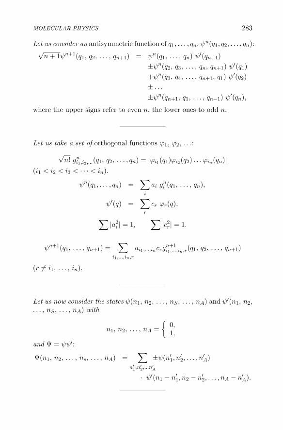
MOLECULAR PHYSICS 283

Let us consider an antisymmetric function of q1, . . . , qn, ψn(q1, q2, . . . , qn):√

n + 1ψn+1(q1, q2, . . . , qn+1) = ψn(q1, . . . , qn) ψ′(qn+1)±ψn(q2, q3, . . . , qn, qn+1) ψ′(q1)+ψn(q3, q4, . . . , qn+1, q1) ψ′(q2)± . . .

±ψn(qn+1, q1, . . . , qn−1) ψ′(qn),

where the upper signs refer to even n, the lower ones to odd n.

——————–

Let us take a set of orthogonal functions ϕ1, ϕ2, . . .:√

n! gni1,i2,...(q1, q2, . . . , qn) = |ϕi1(q1)ϕi2(q2) . . . ϕin(qn)|

(i1 < i2 < i3 < · · · < in).

ψn(q1, . . . , qn) =∑

i

ai gni (q1, . . . , qn),

ψ′(q) =∑

r

cr ϕr(q),

∑|a2

i | = 1,∑

|c2r | = 1.

ψn+1(q1, . . . , qn+1) =∑

i1,...,in,r

ai1,...,incrgn+1i1,...,in,r(q1, q2, . . . , qn+1)

(r �= i1, . . . , in).

——————–

Let us now consider the states ψ(n1, n2, . . . , nS , . . . , nA) and ψ′(n1, n2,. . . , nS , . . . , nA) with

n1, n2, . . . , nA ={

0,1,

and Ψ = ψψ′:

Ψ(n1, n2, . . . , ns, . . . , nA) =∑

n′1,n′

2,...n′A

±ψ(n′1, n

′2, . . . , n

′A)

· ψ′(n1 − n′1, n2 − n′

2, . . . , nA − n′A).

——————–

284 E. MAJORANA: RESEARCH NOTES ON THEORETICAL PHYSICS

Ψ(q1, q2) = −Ψ(q2, q1),

Ψ(q1, q2) =∑

aik ϕi(q1) ϕk(q2),

aik = −aki,∑

|a2ik| = 1;

Ψ(q) =∑

ci ϕi(q),

∑|c2

i | = 1.

Ψ(q1, q2, q) =Ψ(q1, q2)ψ(q) + Ψ(q2, q)ψ(q1) + Ψ(q, q1)ψ(q2)√

3= −Ψ(q2, q1, q) = −Ψ(q1, q, q2) = −Ψ(q, q2, q1)= Ψ(q2, q, q1) = Ψ(q, q1, q2).

√3 Ψ(q1, q2, q) =

∑

i,k,r

aik cr [ϕi(q1)ϕk(q2)ϕr(q) + ϕi(q2)ϕk(q)ϕr(q1)

+ϕi(q)ϕk(q1)ϕr(q2)] .

∫ΨΨ dτ1dτ2dτ =

13

∑

i,k,r;�,m,s

aika�m crcs [δi�δkmδrs + δisδk�δrm

+ δimδksδr� + . . .]

=∑

i,k,r;�,m,s

aika�m [δi�δkmδrs + δisδk�δrm

+ δimδksδr�] crcs

=∑

r,s

Ars crcs.

Ars =∑

i,k

aikaik δrs +∑

k

askakr +∑

i

aisari

= δrs +∑

i

(aisari + airasi)

= δrs +∑

i

(asiair + ariais),

MOLECULAR PHYSICS 285

Ars = δrs − 2∑

i

asiari

by using aik = −aki.

Ars = δrs − Lrs,

L = AA.

——————–

Without interaction we have:

aik = −2πi

h

∑

�

(Hi�alk + Hk�ai�),

¯aik =2πi

h

∑

�

(Hi�a�k + Hk�ai�).

[14]

ddt

∑

i

(asiari) = −2πi

h

∑

i,�

(asia�iHr� + asiar�Hi� − a�iariHs� − as�ariHi�).

Krs =∑

i

asiari,

[15]

∂

∂tKrs = −2πi

h

∑

�

(K�sHr� − Kr�H�s),

K = −2πi

h(KH − HK).

14@ In the following expression appearing in the original manuscript, the author pointed outthe cancellation of the second and fourth term in the sum.15@ In the original manuscript, some signs in the following expressions were incorrect.

5

STATISTICAL MECHANICS

5.1. DEGENERATE GAS

A degenerate gas of spinless electrons in a box of length L is consideredin the following. The electrostatic interaction between the particles istaken into account in a peculiar way.

[1]

For spinless electrons:

ψ�,m,n =1

L3/2e2πi(�x+my+nz)/h =

1L3/2

e2π p·q/h,

T =h2

2L2m(�2 + m2 + n2),

px =h�

L, py =

hm

L, pz =

hn

L.

Ψ =1√N !

∑

±ψ1(q1) · · ·ψn(qn),

ψi = ψ�i,mi,ni.

Aik =∫

e2

r12|ψ2

i (q1)| |ψ2k(q2)| dq1 dq2 = A (independent of i and k),

Iik =∫

e2

r12ψi(q1)ψk(q2)ψi(q2)ψk(q1) dq1 dq2.

1@ In the original manuscript, the unidentified Ref. 8.47 appears here.

287

288 E. MAJORANA: RESEARCH NOTES ON THEORETICAL PHYSICS

∫ΨHΨdτ =

n∑

i=1

Ti +12

∑

i,k

Aik − 12

∑

i,k

Iik,

Aik = A, Iik =e2h2

π|pi − pk|2L3.

5.2. PAULI PARAMAGNETISM

In the following notes the author reported a (preliminary?) study onPauli paramagnetism. He considered an ensemble of N degenerate fer-mions (so that N is proportional to the third power of the Fermi mo-mentum, or V 3/2 where V is the electrostatic potential) interacting witha magnetic field H by means of the Pauli term μ0H, and obtained anexpression for the magnetic susceptibility χ. The number of spin-up andspin-down fermions was denoted with n′ and n′′, respectively.

N

2= kV 3/2.

N = n′ + n′′,

n′ = k (V + μ0H)3/2 � kV 3/2 +32kV 1/2μ0H =

N

2+

32

μ0H

V· N

2,

n′′ = k (V − μ0H)3/2 � kV 3/2 − 32kV 1/2μ0H =

N

2− 3

2μ0H

V· N

2.

n′ − n′′ =32

μ0H

VN,

μ0(n′ − n′′) =32

μ20H

VN.

χ =(n′ − n′′)μ0

H=

32

Nμ2

0

V.

[2]

2@ In the original manuscript some numerical calculations appear here, that probably rep-resent an attempt to evaluate the magnetic susceptibility of sodium Na (considered as an

STATISTICAL MECHANICS 289

5.3. FERROMAGNETISM

In this Section, Majorana studied the problem of ferromagnetism in theframework of the Heisenberg model with the exchange interaction. How-ever, it is rather evident that the Majorana approach is seemingly orig-inal, since he does not follow neither the Heisenberg formulation (seeW. Heisenberg, Z. Phys. 49 (1928) 619) nor the subsequent van Vleckformulation (which followed Dirac) in terms of spin Hamiltonian (seeJ.H. van Vleck, The Theory of Electric and Magnetic Susceptibilities(Oxford University Press, London, 1932). He considered a system of iatoms (located at positions r1, r2, etc.) with spin parallel to the appliedmagnetic field on a total of n atoms, and started by writing the Slater de-terminants A of the atomic wavefunctions ψ with respect to the possiblecombinations of i spin-up atoms out of the n total atoms. The Heisen-berg exchange interaction (which is of electrostatic origin) Vrs amongnearest neighbor atoms (the number of nearest neighbors is denoted witha) was then introduced and the energy E of the system evaluated. Thesubsequent calculations, performed by employing statistical arguments,were aimed to obtain the magnetization of the system (with respect tothe saturation value) when a magnetic field H acts on the magnetic mo-ment μ of each atom. For further discussion, see S. Esposito, preprintarXiv:0805.3057 [physics:hist-ph].

r1, r2, . . . ri ↑ ↑ ↑ . . .

ri+1, . . . rn ↓ ↓ ↓ . . .

A(r1 . . . ri|ri+1 . . . rn) =

∣∣∣∣∣∣∣∣∣∣∣∣∣∣

ψr1(q1)δ(s1 − 1) . . . ψr1(qn)δ(sn − 1). . .

ψri(q1)δ(s1 − 1) . . . ψri(qn)δ(sn − 1)

ψri+1(q1)δ(s1 + 1) . . . ψri+1(qn)δ(sn + 1). . .

ψrn(q1)δ(s1 + 1) . . . ψrn(qn)δ(sn + 1)

∣∣∣∣∣∣∣∣∣∣∣∣∣∣

ensemble of 6 · 1023 (Avogadro’s number) nucleons, or 3 · 1022 nuclei):

V = p · 1, 59 · 10−12 volt,

χ =3

2· 3 · 1022 0, 85 · 10−40

p · 1, 59 · 10−12=

3

2

3 · 0, 85

p · 1, 5910−6.

290 E. MAJORANA: RESEARCH NOTES ON THEORETICAL PHYSICS

Ai(r11, r

12 . . . r1

1|r1i+1, r

1i+2 . . . r1

n). . .

Aτ (rτ1 , . . . . . . rτ

1 |rτi+1, r

τn)

τ =n!

i!(n − i)!

(the order of r1 . . . ri or

ri+1 . . . rn is not important

).

If H is the interaction operator acting on each particle, the electrostaticinteraction potential V0 is given by:

V0 =∫

Hψ1(q1)ψ1(q1)ψ2(q2)ψ2(q2) . . . ψn(qn)ψn(qn) dq1 . . . dqn.

The exchange energy between r and s orbits Vrs:

Vrs =∫

e2

|q1 − q2|ψr(q1)ψs(q1)ψr(q2)ψs(q2) dq1dq2;

Vrs = Vsr.

Hmm = V0 −∑

r<s

Vrs +rmi∑

r=rm1

rmn∑

s=rmi+1

Vrs,

and for m �= n:

Hmn =

⎧⎪⎪⎪⎪⎨

⎪⎪⎪⎪⎩

−Vrs, for a transition from Am to An by exchangingthe opposite intrinsic orientation in the orbitsψr and ψs,

0, for the other cases.

In the ferromagnetic case, if each atom has n neighbor atoms:3

Vrs =

⎧⎨

⎩

ε, (neighbor atoms),

0, (distant atoms).

E = H − V0 +∑

r<s

Vrs = H − V0 +na

2ε.

3@ In the original manuscript, the upper limits of the second sum in the expression for Emm

are both (incorrectly) written as rni .

STATISTICAL MECHANICS 291

Emm =rmi∑

rm1

rmn∑

rmi+1

Vrs = Nm ε,

and for m �= n:

Emn =

⎧⎨

⎩

−Vrs,

0.

Can we consider E as diagonal, in a statistical sense? Let us assumethat it can be.For any given value of N , y solutions exist:

y = y(N).

N

y

In each of the quantities A we exchange randomly an orbit ↑ with a ↓one; the quantities A change into B:

A1 −→ B1

. . .Aτ −→ Bτ

♦

Statistically, the set of B’s coincides with that of the A’s.

y0 = y(N0),

that is, we have y0 quantities A corresponding to N0. If we perform thetransformation ♦, the quantities B corresponding to the y0 quantities Awill be distributed between

N0 − 2a and N0 + 2a,

292 E. MAJORANA: RESEARCH NOTES ON THEORETICAL PHYSICS

and letp2a, N0 + 2a,p2a−2, N0 + 2a − 2,. . .p2, N0 + 2,p0, N0,. . .p−2, N0 − 2,. . .p−2a, N0 − 2a,

be the probabilities that one out of the mentioned B quantities corre-sponds to N = N0 + 2a, or N0 + 2a − 2, etc.We can evaluate the average increment:

ΔN0 =a∑

−a

2r p2r.

In fact, on average an electron ↑ has

N0

ielectrons ↓ and a − N0

ielectrons ↑

as neighbors, while an electron ↓ has

N0

n − ielectrons ↑ and a − N0

n − ielectrons ↓

as neighbors. By performing the mentioned exchange, we evidently have:

ΔN0 = 2a − 2N0

(1i

+1

n − i

).

Let us assume that the probabilities p obey the following law (which wecan call “normal”)

p2r =(

12

+ΔN0

4a

)a+r (12− ΔN0

4a

)a−r (2a)!(a − r)!(a + r)!

.

Assuming that, for a restricted range,

y(N0 + 1) = y0 ek,

. . .

y(N0 ± a) = y0 e±ka,

STATISTICAL MECHANICS 293

the condition that y(N) does not change while we pass from A’s to B’scan be expressed as:

a∑

−a

p2r e−2kr = 1,

which is solved by:

ek =1 +

ΔN0

2a

1 − ΔN0

2a

.

The trivial solution:k = 0

has to be excluded since, although it does not change y = y(N) for shortranges, it gives rise to a non constant “flux” of “radions”4 through anysection N = N0 of the curve y = y(N) when passing from the A’s to theB’s.It follows that, by considering y as a continuous function of N :

y′

y= log

2 − N

a

(1i

+1

n − i

)

N

a

(1i

+1

n − i

) ,

and setting

α =1a

(1i

+1

n − i

)=

n

a i (n − i),

y′

y= log

(2

αN− 1

),

we have

d log y = log(

2αN

− 1)

dN.

t =2

αN− 1,

t + 1 =2

αN,

N =2

α(t + 1),

4@ We find the original text quite obscure.

294 E. MAJORANA: RESEARCH NOTES ON THEORETICAL PHYSICS

dN = − 2α(t + 1)2

dt;

d log y = − log t · 2α(t + 1)2

dt.

log y =2α

log t

(t + 1)− 2

α

∫dt

t(t + 1)

=2α

log t

t + 1− 2

αlog t +

2α

log(t + 1) + k

=2α

log2

αN− 2

α

(1 − αN

2

)log

(2

αN− 1

)+ k,

y = c

(2

αN

) 2α

(2

αN− 1

)− 2α

+N

,

or

y = c

(2

2 − αN

) 2α

(2

αN− 1

)N

,

ory = c (t + 1)

2α t−

2α

+N = c (t + 1)2α t

− 2α

+ 2α(t+1) ;

y(0) = c = y

(2α

)= c, y

(2α

+ ε2

)= 0.

∫y dN ∼=

∫y

(1α

)e−αN ′2

dN ′ =√

π

αy

(1α

)=

√π

αc 2

2α .

Since the number of solutions is(

ni

), we have:

c =(

ni

) √1π

n

a i (n − i)1

22i(n−i)a

n

=

√1aπ

√n

i(n − i)

(12

)a·2i(n−i)n

(ni

)=

(ni

)12

2α

√α

π.

STATISTICAL MECHANICS 295

y = c

(2

αN

) 2α

(2

αN− 1

)− 2α

+N

,

y = c

(2

2 − αN

) 2α

(2

αN− 1

)N

.

——————–

Numerical example:

n = 10, i = 3, a = 4,

(ni

)= 120, α =

542

,2α

= 16.8,

c = 0.0002046,

[5]

y = 0.0002046(

16.8N

)16.8 (16.8N

− 1)−16.8+N

,

y = 0.0002046(

16.816.8 − N

)16.8 (16.8N

− 1)N

.

[6]

5@ Note that the correct value of c is 0.0002047.6@ The following table lists some values of y for given N (for example, 0 or 16.8, 1 or 15.8,etc.) as calculated from the previous expressions. Note, however, that the (complete) correctnumerical values should be as:

N y

0 − 16.8 0.00021 − 15.8 0.00912 − 14.8 0.0943 − 13.8 0.544 − 12.8 2.075 − 11.8 5.666 − 10.8 11.657 − 9.8 18.478 − 8.8 22.908.4 23.35

296 E. MAJORANA: RESEARCH NOTES ON THEORETICAL PHYSICS

N y

0 − 16.8 0.00021 − 15.8 0.00882 − 14.8 0.0893 − 13.84 − 12.85 − 11.8 5.696 − 10.87 − 9.8 18.458 − 8.88.4 23.35

——————–

We can also write:

y = c 22α (1 − α2N ′2)−

1α

(1 − αN

1 + αN

)N ′

,

whereN ′ = N − 1

α,

which points out the symmetry property.

log y = k − 1α

log(1 − α2N ′2) + N ′ log1 − αN ′

1 + αN ′ .

log(1 − αN ′) = −αN ′ − 12α2N ′2 − 1

3α3N ′3 − . . . ,

log(1 + αN ′) = αN ′ − 12α2N ′2 +

13α3N ′3 + . . . ;

log(1 − α2N ′2) = −α2N ′2 − 12α4N ′4 − . . . ,

log1 − αN ′

1 + αN ′ = −2αN ′ − 23α3N ′3 − . . . ;

log y = k − αN ′2 − 16α3N ′4 − 1

15α5N ′6 − 1

28α7N ′8 − 1

45α9N ′10 − . . . .

e−WkT = e−

NεkT = e−LN = Ce−LN ′

,

L =ε

kT, C = e−

Lα .

STATISTICAL MECHANICS 297

log(y e−WkT ) = k + log C − LN ′ − αN ′2 − 1

6α3N ′4 − 1

15α5N ′6 − . . .

= k + log C − LN ′ − 1α

log(1 − α2N ′2) + N ′ log1 − αN ′

1 + αN ′ .

ddN

log(y e−

WkT

)= −L + log

1 − αN ′

1 + αN ′ = −L + log(

2αN

− 1)

,

d2

dN2log

(y e−

WkT

)= − 2

αN2

αN

2 − αN= − 2

N(2 − αN)=

2α

(1 − α2N ′2);

(y e−

WkT

)

max= y0 e−

W0kT ,

−1 +2

αN0= eL,

2αN0

= eL + 1,

N0 =2

α(eL + 1),

αN =2

eL + 1,

2 − αN ==2eL

eL + 1,

αN(2 − αN) =4eL

(eL + 1)2.

y0 = c

(eL + 1

eL

) 2α

eLN0 ,

y0 e−WkT = e−LN0 c

(eL + 1

eL

) 2α

eLN0 = c

(eL + 1

eL

) 2α

.

y e−WkT = c

(eL + 1

eL

) 2α

e−(eL+1)2

4eL α(N−N0)2.

298 E. MAJORANA: RESEARCH NOTES ON THEORETICAL PHYSICS

∫y e−

WkT dN =

∫y dN ·

(eL + 12eL

) 2α

√4eL

(eL + 1)2

=∫

y dN ·(

1 + e−L

2

) 2α 2

√eL

eL + 1

=(

ni

)(1 + e−L

2

) 2α 2

√eL

eL + 1

=(

ni

)(1 + e−L

2

)a2i(n−i)

n 2√

eL

eL + 1.

M =μH

kT.

↑ ↑ ↑ . . . ↑1 2 3 i

↓ ↓ ↓ . . . ↓i + 1 i + 2 i + 3 n

The ratio S between the magnetic moment under the influence of thefield H and the saturation magnetic moment is:

S =

∑ 2i

n

(ni

)(1 + e−L

2

)a2i(n−i)

n

eM2i[e−Mn

]

∑(ni

)(1 + e−L

2

)a2i(n−i)

n

eM2i[e−Mn

]− 1.

log∫

e−WkT eM(2i−n)y dN

= a2i(n − i)

nlog

1 + e−L

2+ 2Mi − i log i − (n − i) log(n − i) + const.

⊕

By taking the derivative with respect to i and equating the result to 0:

a2(n − 2i)

nlog

1 − e−L

2+ 2M − log i− � 1 + log(n − i)+ � 1 = 0,

logi

n − i= 2M + a

2(n − 2i)n

log1 + e−L

2.

⊗

STATISTICAL MECHANICS 299

S′ =2i − n

n=

2i

n− 1,

2i

n= 1 + S′,

i

n=

1 + S′

2;

n − i

n=

1 − S′

2.

log1 + S′

1 − S′ = 2M − 2aS′ log1 + e−L

2.

It follows:

log1 + S′

1 − S′ = 2μ

kTH + 2aS′ log

21 + e−

εkT

.

For small H and large T :

2S = 2μ

kTH + 2aS log

21 + e−

εkT

.

For T lower7 than the Curie point: for a given value of H there exist 2values of S which, for not extremely high H, are practically equal andopposite.From

⊗it follows:

a2i(n − i)n

log1 + e−L

2=

(log

i

n − i− 2M

)i

n − i

n − 2i.

Substituting in⊕

:

−2Mii

n − 2i+ log i · i2

n − 2i− log(n − i) · (n − i)2

n − 2i.

Let us set (y > 0):

log1 + y

1 − y= 2ay log

21 + e−

εkT

,

log1 + y + Δy

1 − y − Δy= 2

μ

kTH + 2a(y + Δy) log

21 + e−

εkT

,

7@ We find the original text to be quite obscure, and our own interpretation is only a probableone.

300 E. MAJORANA: RESEARCH NOTES ON THEORETICAL PHYSICS

Δy

1 − y2=

μ

kTH + a log

21 + e−

εkT

Δy,

[8]

Δy =

μH

kT1

1 − y2− a log

21 − e−

εkT

.

The LHS in⊕

can also be written as:

a1 − S′2

2n log

1 + e−L

2+ M(1 + S′)n − n

1 + S′

2log n

1 + S′

2

−n1 − S′

2log n

1 − S′

2+ const.

=(

a1 − S′2

2log

1 + e−L

2MS′ − 1 + S′

2log

1 + S′

2

−1 − S′

2log

1 − S′

2

)+ const.

5.4. FERROMAGNETISM: APPLICATIONS

In the following, the author gives some examples of ferromagnetic ma-terials with different geometries (corresponding to different numbers iof oriented spins on a total of n, and to different numbers a of nearestneighbors). Three insert also appear, mainly aimed at evaluating sometheoretical quantities related to spontaneous magnetization.

a = 3, i = 3, n − i = 3;(

ni

)= 20.

8@ In the original manuscript, the following formula is incorrectly written as:

Δy =

μH

kT

1 − y2 − a log2

1 − e−ε

kT

.

STATISTICAL MECHANICS 301

1, 2, 3 5 52, 3, 4 5 33, 4, 5 5 54.5, 6 5 55, 6, 1 5 36, 1, 2 5 5

1, 2, 4 5 51, 2, 5 5 52, 3, 5 5 72, 3, 6 5 53, 4, 6 5 53, 4, 1 5 74, 5, 1 5 54, 5, 2 5 55, 6, 2 5 75, 6, 3 5 56, 1, 3 5 56, 1, 4 5 7

1, 3, 5 9 72, 4, 6 9 7

18 52 9

ff

5.4

2 312 56 7

9

=

;

5.4

18 · 0.42 + 2 · 3.62 = 28.8

2 · 2.42 + 12 · 0.42 + 6 · 1.62 = 28.8

N y1 y2 Ny1 Ny2 N2y1 N2y2 N3y1 N3y2

3 2 6 18 545 18 12 90 60 450 300 2250 15007 6 42 294 20589 2 18 162 1458

20 20 108 108 612 612 3708 3612

——————–

Mean value:a i(n − i)

n − 1=

1α

,

3 · 3 · 35

= 5.4.

302 E. MAJORANA: RESEARCH NOTES ON THEORETICAL PHYSICS

(a

n−1

)2, i−1

in−i−1

n−i = ni−i2−n+1i(n−i) ,

an−1

a−1n−2 , 1

in−i−1

n−i + i−1i

1n−i = n−2

i(n−i) ,

an−1 , 1

i(n−i) .

1) −

2) n−1n

n−2n

n−3n

[i(n−i)−(n−1)]n3

i(n−i)(n−1)(n−2)(n−3)i(n−i)−(n−1)

i(n−i) ,

3) n−1n

n−2n

4n

[i(n−i)−(n−1)]n3

i(n−i)(n−1)(n−2)(n−3)[i(n−i)−(n−1)]

i(n−i)4

n−3 ,

4) n−1n

2n

1n

[i(n−i)−(n−1)]n3

i(n−i)(n−1)(n−2)(n−3)i(n−i)−(n−1)

i(n−i)2

(n−2)(n−3) .

a2 [i(n − i) − (n − 1)]ni(n − i)(n − 1)(n − 2)(n − 3)

+1

i(n − i)n

n − 1a − 1n − 2

[n − 2 − 4

i(n − i) − (n − 1)n − 3

]

+1

i(n − i)a

n − 1

[1 − 2

i(n − i) − (n − 1)(n − 2)(n − 3)

]

=1

i(n − i)(n − 1)(n − 2)(n − 3){a2n [i(n − i) − (n − 1)]

+a(a − 1)(n − 2)(n − 3) − 4a(a − 1) [i(n − i) − (n − 1)]+a(n − 2)(n − 3) −2a [i(n − i) − (n − 1)]}

=(a2n − 4a2 + 2a)[i(n − i) − (n − 1)] + a2(n − 2)(n − 3)

i(n − i)(n − 1)(n − 2)(n − 3).

Mean value of the square of the terms in the diagonal:

i(n − i)(a2n − 4a2 + 2a)[i(n − i) − (n − 1)] + a2(n − 2)(n − 3)

(n − 1)(n − 2)(n − 3)

= 3 · 3 · 24 · 4 + 10860

=183660

= 30.6 =61220

=a2

(n − 1)2i2(n − i)2 +

4n − 6(n − 2)(n − 3)

a2

(n − 1)2i2(n − i)2

− 4n − 4(n − 2)(n − 3)

a2

(n − 1)2i2(n − i)2

+2a

(n − 2)(n − 3)1

n − 1i2(n − i)2 − a2n

(n − 2)(n − 3)i(n − i)

+4a2

(n − 2)(n − 3)i(n − i) − 2a

(n − 2)(n − 3)i(n − i) +

a2

n − 1i(n − i).

STATISTICAL MECHANICS 303

[9]

terms in the diagonal eigenvalues

meanvalue

ai(n−i)n−1

ai(n−i)n−1

meanvalue of thesquare

a2i2(n−i)2

(n−1)2+ k2 a2i2(n−i)2

(n−1)2+ k2 + ai(n−i)

n−1

Statistically:

terms in the diagonal eigenvalues

meanvalue

ai(n−i)n

ai(n−i)n

meanvalue of thesquare

a2i2(n−i)2

n2 + 2ai2(n−i)2

n3a2i2(n−i)2

n2 + 2ai2(n−i)2

n3 + ai(n−i)n

——————–

n = 24, i = 6, a = 2;(

ni

)= 134596.

9@ In the original manuscript, there appears here the matrix:˛

˛

˛

˛

˛

˛

V4 + V5 −V5 −V4

−V5 V5 + V6 −V4

−V4 −V4 V6 + V4

˛

˛

˛

˛

˛

˛

,

whose meaning is unclear to us.

304 E. MAJORANA: RESEARCH NOTES ON THEORETICAL PHYSICS

[10]

y N yN N − N0 (N − N0)2 y(N − N0)2

20412 12 244944 2.61 6.8 13900068040 10 680400 0.61 0.4 2600034020 8 272160 −1.39 1.9 650009072 6 54432 −3.39 11.5 1040003024 4 12096 −5.39 29 88000

28 0 0 −9.39 88 2000134596 1264032 424000

1 9.3913 3.15

9.3913 =21623

=2 · 6 · 18

23,

3.15 � 2 · 2 · 36 · 324243

= 3.375.

——————–

n = 60, i = 10, a = 1, n − i = 50.

[11]

10@ The numbers in the last line of the following table are the mean values of y, yN andy(N −N0)2, respectively, which are obtained by dividing the numbers in the previous line by134596.11@ See the previous footnote. The symbols introduced below have the following meaning:according to what is asserted in the original manuscript:

y† = y

ffi„

3010

«

· 210 , yN‡ = yN

ffi„

6020

«

· 210,

y(N − N0)2§

= y(N − N0)2ffi„

3010

«

· 210.

STATISTICAL MECHANICS 305

y† N yN ‡ N − N0 (N − N0)2 y(N − N0)2§

1 10 10 1.52 2.31 2.311.071 8 8.57 −0.48 0.23 0.250.341 6 2.05 −2.48 6.15 2.100.037 4 0.15 −4.48 20 0.740.001 2 −6.48 42 0.040 0 −8.48 722.450 20.77 5.44

1 8.48 2.22

1 · 2 · 100 · 2500216000

= 2.31.

——————–

(ni

)∼=

√n

2π

nn i−i (n − i)−(n−i)

√i√

n − i=

k

ii (n − i)n−i√

i√

n − i,

k =√

n

2πnn.

Pi solutions with apparent momentum n − 2i,

Qi solutions with intrinsic momentum n − 2i.

i ≤ n/2.

Pi =i∑

j=0

Qi, Qi = Pi − Pi−1.

pi =(

ni

).

qi = pi − pi−1;

pi−1 = pii

n − i + 1,

qi = pi − pi−1 = pi

(1 − i

n − i + 1

)= pi

n − 2i + 1n − i + 1

,

qi =(

ni

)n + 1 − 2i

n + 1 − i.

306 E. MAJORANA: RESEARCH NOTES ON THEORETICAL PHYSICS

n = 4:i pi ni

0 1 11 4 32 6 2

∑

σ

P σi =

(ni

)a i(n − i)

n,

∑

σ

P σi

2 =(

ni

) [a2i2(n − i)2

n2+

2a i2(n − i)2

n3+

a i(n − i)n

],

∑

σ

Qσi =

∑

σ

P σi −

∑

s

P σi−1

=(

ni

)a i(n − i)

n−

(n

i − 1

)a(i − i)(n − i + 1)

n

=(

ni

)a i(n − 2i + 1)

n,

∑Qi

qi=

a i(n + 1 − i)n

.

——————–

Curves of the eigenvalues corresponding to apparent momentum N −2i:yi = yi(N).For large n, yi tend to the limiting form:

logyi

n= n + n fi

(2

a nN

)= n + nfi(x), x =

2a n

N.

fi(x)max = fi(xi0), xi

0 =2

a n

a i(n − i)n

= 2i

n

n − i

n,

f ′i(x

i0) = 0,

f ′′i (xi

0) = − a

/(41n

n − i

n+ 8

i2

n2

(n − i)2

n2

).

N : μ2 =2a i2(n − i)2

n3+

a i(n − i)n

,

χ : μ′2 =8a i2(n − i)2

a n5+

4i(n − i)a n3

.

STATISTICAL MECHANICS 307

5.5. AGAIN ON FERROMAGNETISM

In the following pages, the author probably comes back again to ferromag-netism, but the meaning is quite obscure to us. See also E. Majorana,Nuovo Cim. 8 (1931) 78.∣∣∣∣∣∣∣∣∣∣∣∣

ψ1(q1) ψ1(q2) . . . ψ1(qn)

ψ2(q1) ψ2(q2) . . . ψ2(qn)

. . .

ψn(q1) ψn(q2) . . . ψn(qn)

∣∣∣∣∣∣∣∣∣∣∣∣

= ψ1(q1)

∣∣∣∣∣∣∣∣∣

ψ2(q1) . . . ψ2(qn)

. . .

ψn(q1) . . . ψn(qn)

∣∣∣∣∣∣∣∣∣

± ψ1(q2)

∣∣∣∣∣∣∣∣∣

ψ2(q3) . . . ψ2(q1)

. . . . . . . . .

ψn(q3) . . . ψn(q1)

∣∣∣∣∣∣∣∣∣

+ . . .n∑

r=1

ϕ(qr+1, qr+2, . . . , qn, q1, . . . , qr−1)ψ(qr), n = 2p + 1.

[12]1 ↑↑↑ 0

2 ↑↑↓ ϕ1(ψ2ψ3) − ϕ2(ψ1ψ3) (123)

3 ↑↓↑ ϕ3(ψ1ψ2) − ϕ1(ψ3ψ2) (132)

4 ↑↓↓ 0

5 ↓↑↑ ϕ2(ψ3ψ1) − ϕ3(ψ2ψ1) (123)

6 ↓↑↓ 0

7 ↓↓↑ 0

8 ↓↓↓ 0ψ, ϕ, u, v.

ψ1ψ2(u1v2−u2v1)ϕ3u3+ψ2ψ3(u2v3−u3v2)ϕ1u1+ψ3ψ1(u3v1−u1v3)ϕ2u2.

12@ In the original manuscript, some pages of scratch calculations appear here: they dealwith combinations of several objects grouped in different ways, probably with an eye on thestudy of ferromagnetism (see below).

PART III

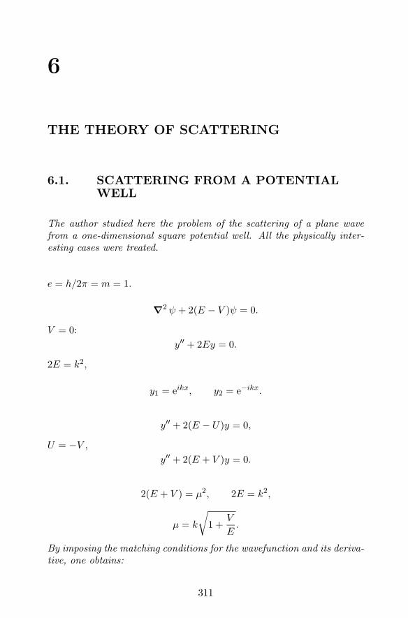
6

THE THEORY OF SCATTERING

6.1. SCATTERING FROM A POTENTIALWELL

The author studied here the problem of the scattering of a plane wavefrom a one-dimensional square potential well. All the physically inter-esting cases were treated.

e = h/2π = m = 1.

∇2 ψ + 2(E − V )ψ = 0.

V = 0:y′′ + 2Ey = 0.

2E = k2,

y1 = eikx, y2 = e−ikx.

y′′ + 2(E − U)y = 0,

U = −V ,y′′ + 2(E + V )y = 0.

2(E + V ) = μ2, 2E = k2,

μ = k

√

1 +V

E.

By imposing the matching conditions for the wavefunction and its deriva-tive, one obtains:

311

312 E. MAJORANA: RESEARCH NOTES ON THEORETICAL PHYSICS

y =

⎧⎪⎪⎪⎪⎪⎪⎪⎪⎪⎪⎪⎪⎪⎪⎪⎨

⎪⎪⎪⎪⎪⎪⎪⎪⎪⎪⎪⎪⎪⎪⎪⎩

1 +√

1 + VE

2eik(x+a)−iμa +

1 −√

1 + VE

2e−ik(x+a)−iμa,

x < −a,

eiμx,

[g = 1 +

12

V

E

]− a < x < a,

1 +√

1 + VE

2eik(x−a)+iμa +

1 −√

1 + VE

2e−ik(x+a)+iμa,

a < x,

E > 0,

E =12

μ2 − V, E =12

k2,

μ = k

√

1 +V

E, k =

μ√

1 + VE

.

√g gives the ratio of the wave amplitude inside and outside the well.1

E < 0, E > −V :

√

1 +V

E= i

√V

−E− 1,

μ = ik

√V

−E− 1 = k1

√V

−E− 1, k1 = ik.

1@ That is: g is given by the ratio a2+b2/c2 where a [b] is the coefficient of the first [second]wave term in the first or third row, while c is the coefficient of the wave term in the secondrow (c = 1). Note that the quantity we call g, here and in what follows, is in the originalmanuscript denoted by y, the same as the symbol there used for the wave function.

THE THEORY OF SCATTERING 313

y =

⎧⎪⎪⎪⎪⎪⎪⎪⎪⎪⎪⎪⎪⎪⎨

⎪⎪⎪⎪⎪⎪⎪⎪⎪⎪⎪⎪⎪⎩

1 + i√

V−E − 1

2ek1(x+a)−iμa +

1 − i√

V−E − 1

2e−k1(x+a)−iμa,

x < −a,

eiμx, − a < x < a,

1 + i√

V−E − 1

2ek1(x−a)+iμa +

1 − i√

V−E − 1

2e−k1(x−a)+iμa,

a < x,

−V < E < 0,

E =12μ2 − V , E = −1

2k2

1,

μ = k1

√V

−E− 1, k1 =

μ√

V−E − 1

.

Stationary states:2

2@ In the original manuscript, there appear here the following calculations:

1 + iq

V−E

− 1

2eiμa = c in = c eniπ/2.

e−iμa

"

cos k(x + a) + i

r

i +V

Esin k(x + a)

#

,

eiμa

"

cos k(x + a) − i

r

i +V

Esin k(x + a)

#

;

− sin μa cos k(x − a) + cos μa

r

1 +V

Esin k(x + a),

cos μa cos k(x − a) − sin μa

r

1 +V

Esin k(x + a).

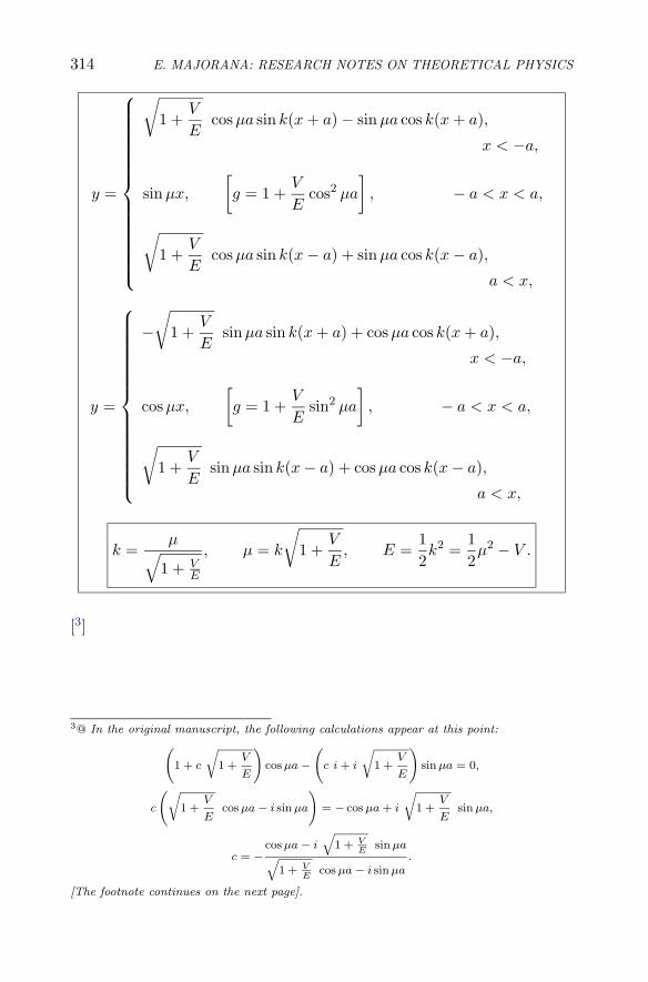
314 E. MAJORANA: RESEARCH NOTES ON THEORETICAL PHYSICS

y =

⎧⎪⎪⎪⎪⎪⎪⎪⎪⎪⎪⎪⎪⎪⎪⎨

⎪⎪⎪⎪⎪⎪⎪⎪⎪⎪⎪⎪⎪⎪⎩

√

1 +V

Ecos μa sin k(x + a) − sin μa cos k(x + a),

x < −a,

sin μx,

[g = 1 +

V

Ecos2 μa

], − a < x < a,

√

1 +V

Ecos μa sin k(x − a) + sinμa cos k(x − a),

a < x,

y =

⎧⎪⎪⎪⎪⎪⎪⎪⎪⎪⎪⎪⎪⎪⎪⎨

⎪⎪⎪⎪⎪⎪⎪⎪⎪⎪⎪⎪⎪⎪⎩

−√

1 +V

Esin μa sin k(x + a) + cos μa cos k(x + a),

x < −a,

cos μx,

[g = 1 +

V

Esin2 μa

], − a < x < a,

√

1 +V

Esin μa sin k(x − a) + cos μa cos k(x − a),

a < x,

k =μ

√1 + V

E

, μ = k

√

1 +V

E, E =

12k2 =

12μ2 − V .

[3]

3@ In the original manuscript, the following calculations appear at this point:

1 + c

r

1 +V

E

!

cos μa −

c i + i

r

1 +V

E

!

sin μa = 0,

c

r

1 +V

Ecos μa − i sin μa

!

= − cos μa + i

r

1 +V

Esin μa,

c = −cos μa − i

q

1 + VE

sin μaq

1 + VE

cos μa − i sin μa.

[The footnote continues on the next page].

THE THEORY OF SCATTERING 315

Reflection

y =

⎧⎪⎪⎪⎪⎪⎪⎪⎪⎪⎪⎪⎪⎪⎪⎪⎪⎪⎨

⎪⎪⎪⎪⎪⎪⎪⎪⎪⎪⎪⎪⎪⎪⎪⎪⎪⎩

[

2

√

1 +V

Ecos 2μa − i

(2 +

V

E

)sin 2μa

]

eik(x+a)

+V

Ei sin 2μa e−ik(x+a), x < −a,

(

1 +

√

1 +V

E

)

eiμ(x−a) −(

1 −√

1 +V

E

)

e−iμ(x−a),

− a < x < a,

2

√

1 +V

Eeik(x−a), a < x,

incident energy: A = 4 + 4V

E+

V 2

E2sin2 2μa,

reflected energy: Ar =V 2

E2sin2 2μa,

refracted energy: AR = 4 + 4V

E,

reflecting power: ρ =Ar

A=

V 2

E2 sin2 2μa

4 + 4VE + V 2

E2 sin2 2μa;

minima: μa = nπ

2.

3

r

1 +V

E+ 1

!

cos μa − i

r

1 +V

E+ 1

!

sin μa =

r

1 +V

E+ 1

!

e−iμa,

r

1 +V

E− 1

!

cos μa + i

r

1 +V

c− 1

!

sin μa =

r

1 +V

E− 1

!

eiμa;

r

1 +V

E

!

e−iμa

,

−

1 −r

1 +V

E

!

eiμa .

316 E. MAJORANA: RESEARCH NOTES ON THEORETICAL PHYSICS

6.2. SIMPLE PERTURBATION METHOD

In the following few passages, Majorana traced the general lines of asimple perturbation method in order to solve the Schrodinger equationfor a particle in a potential field V in terms of the known eigenstates ψi.

∇2 ψ + 2(E − V )ψ = 0.

∇2 ψ0 + 2Eψ0 = 0.

ψ = ψ0 + χ,

∇2 ψ0 + 2(E − V )ψ0 + ∇2 χ + 2(E − V )χ = 0,

∇2 χ + 2(E − V )χ = 2V ψ0.

∇2 ψi + 2(Ei − V )ψi = 0.

2V ψ0 = 2∑

ciψi,

∇2 χ + 2(E − V )χ = 2∑

ciψi.

χ =∑

diψi,

∇2 ψi + 2(E − V )ψi = 2(E − Ei)ψi;

∇2 χ + 2(E − V )χ = 2∑

di(E − Ei)ψ,

di =ci

E − Ei.

THE THEORY OF SCATTERING 317

6.3. THE DIRAC METHOD

The author applied the perturbation theory to the problem of the scat-tering of a particle of momentum p = hγ from a potential V ; the free-particle wavefunction is denoted with φγ. Some approximated expres-sions for the transition probability were obtained within the frameworkof the Dirac method, which are subsequently applied to the particularcase of Coulomb scattering.

E =1

2mp2 + V

=h2

2mγ2 + V.

φγ = e2πi(γxx+γyy+γzz) e−2πi(h/2m)γ2t,

<γ′|V |γ′′>=∫

φγ′ V φγ′′dxdydz = kγ′γ′′ e−2πi(h/2m)(γ′′2−γ′2)t

= kγ′γ′′ e2πi(h/2m)(γ′2−γ′′2)t.

ψ =∫

αγ φγ dγ,

αγ = − 2πi

h

∫kγ′γ′′ e2πi(h/2m)(γ2−γ′2)t αγ′ dγ′.

For t = 0 4:αγ = δ (γ − γ0) .

For t > 0:1st approximation:

αγ = − 2πi

hkγγ0 e2πi(h/2m)(γ2−γ2

0)t,

αγ = − 2m

h2(γ2 − γ20)

kγγ0

(e2πi(h/2m)(γ2−γ2

0)t − 1)

+ δ (γ − γ0) .

4@ Here the author denotes with γ0 = p0/h the momentum (divided by h) of the free particle,while δ(x) signifies the Dirac delta-function.

318 E. MAJORANA: RESEARCH NOTES ON THEORETICAL PHYSICS

2nd approximation:

αγ = − 2πi

hkγγ0 e2πi(h/2m)(γ2−γ2

0)t +4πim

h3

∫kγγ′kγ′γ0

1γ′2 − γ2

0

×(e2πi(h/2m)(γ2−γ2

0)t − e2πi(h/2m)(γ2−γ′2)t)

dγ′,

αγ = − 2m

h2(γ2 − γ20)

kγγ0

γ2 − γ20

(e2πi(h/2m)(γ2−γ2

0)t − 1)

+4m2

h4

∫kγγ′kγ′γ0

(e2πi(h/2m)(γ2−γ2

0)t − 1(γ2 − γ2

0)(γ′2 − γ20)

−e2πi(h/2m)(γ2−γ′2)t − 1(γ2 − γ′2)(γ′2 − γ2

0)

)

dγ′ + δ (γ − γ0) .

In first approximation, for γ �= γ0, we have:

|αγ |2 =16m2

h4(γ2 − γ20)2

|kγγ0 |2 sin2 πh(γ2 − γ2

0)t2m

.

Neglecting constant terms, for t → ∞ we get:

|αγ |2 =8π2m

h3|kγγ0 |

2 t δ(γ2 − γ2

0

),

and the transition probability is:

Pγ0γ =8π2m

h3|kγγ0 |

2 δ(γ2 − γ2

0

).

In second approximation:

|αγ |2 =16m2

h4(γ2 − γ20)2

|kγγ0 |2 sin2 πh(γ2 − γ2

0)t2m

+32m3

h6(γ2 − γ20)

sinπh(γ2 − γ2

0)t2m

∫ (kγγ0kγγ′kγ′γ0 + kγγ0kγγ′kγ′γ0

)

×(

sin πh(γ2 − γ′2)t/2m

(γ2 − γ′2)(γ′2 − γ20)

− sin πh(γ2 − γ20)t/2m

(γ2 − γ20)(γ′2 − γ2

0)

)dγ′.

6.3.1 Coulomb FieldFor a Coulomb field:

V =C

r=

∫Vγ e2πi(γxx+γyy+γzz) dxdy dz,

THE THEORY OF SCATTERING 319

Vγ = C

∫e−2πiγ ·q

rdq = C

∫ ∞

0

2γ

sin 2πγr dr =C

πγ2;

kγ′γ′′ = Vγ′−γ′′ =C

π|γ′ − γ′′|2 .

In first approximation:

Pγ0γ =8mC2

h3|γ − γ0|4δ(γ2 − γ2

0

)=

mC2

2h3γ40 sin4 θ/2

δ(γ2 − γ2

0

).

In second approximation, for γ �= γ0: 5

αγ = −2m

h2

1γ2 − γ2

0

C

π(γ − γ0)2(e2πi(h/2m)(γ2−γ2

0)t − 1)

+4m2

h4

∫C2

π2|γ − γ′|2|γ′ − γ0|2

(e2πi(h/2m)(γ2−γ2

0)t − 1(γ2 − γ2

0)(γ′2 − γ20)

−e2πi(h/2m)(γ2−γ′2)t − 1(γ2 − γ′2)(γ′2 − γ2

0)

)

dγ′.

6.4. THE BORN METHOD

The scattering from a given center was studied here by means of the Bornmethod, and approximated expressions for the scattered partial waveswere obtained.

∇2 ψ + k2ψ = Fψ.

ψ = ψ0 + ψ1 + ψ2 + . . . ,

∇2 ψ0 + k2ψ0 = 0,

∇2 ψ1 + k2ψ1 = Fψ0,

∇2 ψ2 + k2ψ2 = Fψ2,

. . . ,

∇2 ψn + k2ψn = Fψn−1,

. . . .

5@ Probably, the author started to evaluate the transition probability for Coulomb scatteringin a second approximation, but succeeded only in obtaining an expression for the coefficientαγ .

320 E. MAJORANA: RESEARCH NOTES ON THEORETICAL PHYSICS

ψn(q) = − 14π

∫eik|q−q′|

|q − q′| F (q′) ψn−1(q′) dq′.

ψ0(q) = eiku0·q,

ψ1(q) = − 14π

∫eik|q−q′|

|q − q′| eiku0·q′F (q′) dq′,

ψ2(q) =1

16π2

∫∫eik|q−q′|

|q − q′|eik|q′−q′′|

|q′ − q′′| eiku0·q′′F (q′) F (q′′) dq′ dq′′,

|u0| = 1.|q| = r → ∞:

ψ1(q) = − 14πr

∫eik|q−q′| eiku0·q′

F (q′) dq′.

|q| = r, q = r u, |u| = 1;

|q′| = r′, q′ = r′ u′, |u′| = 1,

r → ∞:|q − q′| = r − r′u · u′,

ψ1(q) = −eikr

4πr

∫eikr′(u0−u)·u′

F (q′) dq′.

ψ2(q) =eikr

16π2r

∫∫eik|q′−q′′|

|q′ − q′′| eikr′′u0·u′′eikr′u′·u F (q′) F (q′′) dq′ dq′′.

q′′ = q′ + �:

ψ2(q) =eikr

16π2r

∫eik(u0−u)·q′

F (q′) dq′∫

eik|�|

|�| eiku0·� F (q′ + �) d�.

F =12π

∫Fγ eiγ·q dγ,

Fγ =∫

F e−iγ ·q dq,

∫e−iγ ·q eikr

rdq =

4π

γ2 − k2,

THE THEORY OF SCATTERING 321

r → ∞:

ψ1(q) = −eikr

4πFk(u−u0),

ψ2(q) =eikr

16π2r

∫eik(u0−u)·q′

F (q′) dq′∫

2|ku0 + γ|2 − k2

Fγ eiγ·q′dγ

=eikr

16π2r

∫2

|ku0 + γ|2 − k2Fγ dγ

∫ei(ku0−ku+γ)·q′

F (q′) dq′,

ψ2(q) =eikr

8π2r

∫FγFk(u−u0)−γ

|ku0 + γ|2 − k2dγ

ψ2(q) =eikr

8π2r

∫Fγ−ku0Fku−γ

γ2 − k2dγ.

6.5. COULOMB SCATTERING

The Schrodinger equation for the scattering of a wave from a Coulombpotential is solved and, in particular, the phase advancement is evaluated.

Ze charge of the scatterer;

Z ′e charge of the incident particle;

M mass of the incident particle.

We adopt units such that M = 1, ZZ ′e2 = 1, h/2π = 1. It follows that:

the length unit is h2/4π2MZZ ′e2 = (m/M) (1/ZZ ′) a0; 6

the energy unit is 4π2MZ2Z ′2e4/h2 = 2(M/m) Z2Z ′2 Rh; 7

the velocity unit is 2πZZ ′e2/h = ZZ ′/137c, where 1/137 =e2/(1/2π)hc.

The Schrodinger equation is:

∇2 ψ + 2(

E − 1r

)ψ = 0.

6Here m denotes the electron mass and a0 � 0.529 · 10−9 the Bohr radius.71 Rh = 13.54 V [Remember that the symbol V used by Majorana should more appropriatelyunderstood as eV].

322 E. MAJORANA: RESEARCH NOTES ON THEORETICAL PHYSICS

ψ =n∑

�=0

α�X�(r)

rP�(cos θ),

X ′′� +

(k2 − 2

r− �(� + 1)

r2

)X� = 0,

k2 = 2E (the velocity of the ingoing particle in large units is v =(ZZ ′/137)c k).

X� = X 1� + X 2

� ,

X 1� = x�+1 eikx F

(� + 1 +

i

k, 2� + 2, −2ikx

),

X 2� = x�+1 e−ikx F

(� + 1 − i

k, 2� + 2, 2ikx

),

F (α, β, x) = 1 +α

βx +

α(α + 1)2!β(β + 1)

x2 +α(α + 1)(α + 2)

3!β(β + 1)(β + 2)x3 + . . . .

Alternative solution

X ′′ +(

k2 − 2r− �(� + 1)

r2

)X = 0,

� takes non-integer values greater than −1/2,

X = r�+1 u,

u′′ + 2� + 1

ru′ +

(k2 − 2

r

)u = 0.

[8]

u′′ +(

δ0 +δ1

r

)u′ +

(ε0 +

ε1r

)u = 0,

δ0 = 0, δ1 = 2(� + 1), ε0 = k2, ε1 = −2:

u ∼∫

eiktr (t − 1)�+i/k (t + 1)�−i/k dt.

8@ This equation is a particular case of the more general one reported just after it, and isalso considered by the author in another place; see Appendix 6.10.

THE THEORY OF SCATTERING 323

[...]9

|Im log(1 − t)| ≤ π, |Im log(1 + t)| ≤ π:

u =∫ 1

−1eiktr (1 − t)�+i/k (1 + t)�−i/k dt .

For r = 0, on setting 1 − t = 2x:

u(0) =∫ 1

−1(1 − t)�+i/k (1 + t)�−i/k dt =

∫ 1

0(2x)�−i/k (2 − 2x)�+i/k 2dx

= 22�+1

∫ 1

0(x)�−i/k (1 − x)�+i/k dx,

u(0) = 22�+1 Γ (� + 1 − i/k) Γ (� + 1 + i/k)Γ (2� + 2)

. (1)

|r| > 0:

u = u1 + u2,

u1 = e−i(π/2)(�+1+i/k) eikx

∫ ∞

0e−krp p�+i/k (2 + ip)�−ik dp,

u2 = ei(π/2)(�+1−i/k) e−ikx

∫ ∞

0e−krp p�−+i/k (2 − ip)�+ik dp.

For real r we have u2 = u1.

u1 = (kr)−(�+1) e−i(π/2)(�+1+i/k)−(i/k) log kr eikr

×∫ ∞

0e−p p�+i/k (2 + ip/kr)�−ik dp.

For r → ∞:

u1 = (kr)−(�+1) eπ/2k e−i(π/2)(�+1) eikr−(i/k) log kr 2�−i/k Γ(� + 1 + i/k)

= 2�(kr)−(�+1) eπ/2k e−i(π/2)(�+1) eikr−(i/k) log 2kr Γ(� + 1 + i/k).

Now, replace � with � − ε�; the phase advancement becomes then:

k� = ε�π

2− arg

Γ(� + 1 + i/k)Γ(� + 1 − ε� + i/k)

.

9@ The author then evaluates u′ and u′′ and verifies that the assumed form for u satisfiesthe previous differential equation.

324 E. MAJORANA: RESEARCH NOTES ON THEORETICAL PHYSICS

1/4 > a > 0:

(� − ε�) (� + 1 − ε�) = � (� + 1) − a,(

� +12− ε�

)2

=(

� +12

)2

− a,

ε� = � +12−

√(� +

12

)2

− a.

6.6. QUASI COULOMBIAN SCATTERINGOF PARTICLES

Let us assume a scattering potential of the form:

k√r2 + a2

, (1)

a being the magnitude of the radius of the scatterer. By denoting withT the kinetic energy of the incident particles, let us define the minimumapproach distance10 b in the limit Coulomb field (a = 0) as:

k

b= T ; b =

k

T. (2)

The scattering intensity under an angle θ will be obtained on multi-plying that appearing in the Rutherford formula by a numerical factordepending on the mutual ratios of a, b, λ/2π (λ being the wavelength ofthe free particle) and θ. Let us set:

i = f(α, β, θ) iR, (3)

where iR is the intensity calculated from the Rutherford formula (a = 0)and

α =a

λ/2π, β =

b

λ/2π. (4)

Since for a = 0 the Rutherford formula is exact, we have:

f(0, β, θ) = 1. (5)

10@ That is, the scattering parameter.

THE THEORY OF SCATTERING 325

Let us now consider a fixed α and take the limit β → 0. At zeroth orderapproximation, i.e., exactly for β = 0, we can use the Wentzel method.By choosing as mass unit M , wavelength unit λ/2π and velocity unit vfor the incident particles, from λ = h/Mv it follows that h = 2π in ourunits. Moreover, the kinetic energy of the incident particle is 1/2.From Eqs. (4) and (2) it follows that b = β, k = β/2 and a = α. Bysubstituting these into Eq. (1), we get the expression for the potentialenergy, and the Schrodinger equation corresponding to the eigenvalue1/2 will be:

∇2 ψ +(

1 − β√r2 + α2

)ψ = 0. (6)

Let us set:ψ = ψ0 + ψ1 + ψ2 + . . . ,

where:

∇2 ψn + ψn =β√

r2 + α2ψn−1. (7)

In order to avoid convergence problems, instead of β/√

r2 + α2 let usconsider the expression β

(1/

√r2 + α2 − 1/R

)for r < R and 0 for r >

R; in the final results we will take the limit R → ∞. Eq. (7) is thenreplaced by: 11

∇2 ψn + ψn = P ψn−1; (8)

P =

⎧⎪⎪⎨

⎪⎪⎩

β

(1√

r2 + α2− 1

R

), for r < R;

0, for r > R.

Setting ψ0 = eiz, we have:

∇2 ψ1 + ψ1 = P eiz. (9)

For an univocal solution of Eq. (9) we will choose ψ1 to represent adiverging wave. In this case Eq. (9) can be integrated and, putting

r12 =√

(x − x′)2 + (y − y′)2 + (z − z′)2,

11@ In the original manuscript, the factor β is lacking.

326 E. MAJORANA: RESEARCH NOTES ON THEORETICAL PHYSICS

we get:

ψ1(x, y, z) = − 14π

∫P (x′, y′, z′)

ei(r12+z′)

r12dx′dy′dz′. (10)

Assuming the point (x, y, z) to be far from the origin, we have (r is thedistance from the origin, θ the angle between the vector radius and thez-axis):

r → ∞ : ψ1(r, θ) = − 14πr

∫P (x′, y′, z′) eir

× eir′(cos θ′−cos θ cos θ′−sin θ sin θ′ cos φ′) dx′dy′dz′,

cos θ′(1 − cos θ) − sin θ sin θ′ cos φ′

= 2 sin θ/2[sin θ/2 cos θ′ − cos θ/2 sin θ′ cos φ′]

= 2 sin θ/2[cos (π/2 − θ/2) cos θ′ + sin (π/2 − θ/2) sin θ′ cos

(φ′ − π

)],

r → ∞ : ψ1(r, θ) = − eir

2 r sin θ/2

∫ ∞

0r′P (r′) sin

(2 sin θ/2 r′

)dr′,

(11)whence we easily deduce:

f(α, 0, θ) =2β

sin θ/2∫ ∞

0r′P (r′) sin

(2 sin θ/2 r′

)dr′. (12)

In we simply replace P with β/√

r2 + α2, the integral in Eq. (12) doesnot converge; however, we can circumvent this difficulty by keeping in-determinate the upper integration limit and assuming, for the resultingintegral, its mean value which for the upper limit tends to infinity. Wethus find:

f(α, 0, θ) = 2 sin θ/2∫ ∞

0

r√r2 + α2

sin (2 sin θ/2 r) dr

=∫ ∞

0

x sin xdx√

x2 + 4α2 sin2 θ/2= ϕ (α sin θ/2) .

(13)

THE THEORY OF SCATTERING 327

6.6.1 Method Of The Particular Solutions

u′′� +

(1 − β√

r2 + α2− �(� + 1)

r2

)u� = 0. (14)

For the hydrogen atom we consider the values β = 0.4, 0.5, 0.6, 0.7and α = 0, 0.2, 0.4, 0.6, 0.8, 1. The solution of Eq. (14) is reportednumerically in the following tables for � = 0 and β = 0.4. 12

α = 0 α = 0.2 α = 0.4r0

0.1

0.2

0.3

0.4

0.5

0.6

0.7

0.8

0.9

1.0

1.1

1.2

1.3

u u′ u′′

0 1 0.4001.019

0.1018 0.3051.049

0.2067 0.2071.070

0.3137 0.1091.080

0.4217 0.0001.080

0.5297 -0.1061.069

0.6366 -0.212

u u′ u′′

0 1 0u u′ u′′

0 1 0

12@ The author uses a numerical algorithm (unknown to us) in order to infer the solutionu(r) of Eq. (14) from its second (and first) derivative, and the first few results obtained aredisplayed in the tables.

328 E. MAJORANA: RESEARCH NOTES ON THEORETICAL PHYSICS

α = 0.6 α = 0.8 α = 1.0r0

0.1

0.2

0.3

0.4

0.5

0.6

0.7

0.8

0.9

1.0

1.1

1.2

1.3

u u′ u′′

0 1 0u u′ u′′

0 1 0u u′ u′′

0 1 0

6.7. COULOMB SCATTERING: ANOTHERREGULARIZATION METHOD

Let us assume the potential to be as follows:

V =

{V0, for r < R,

k/r, for r > R.(1)

r

V

R

V0

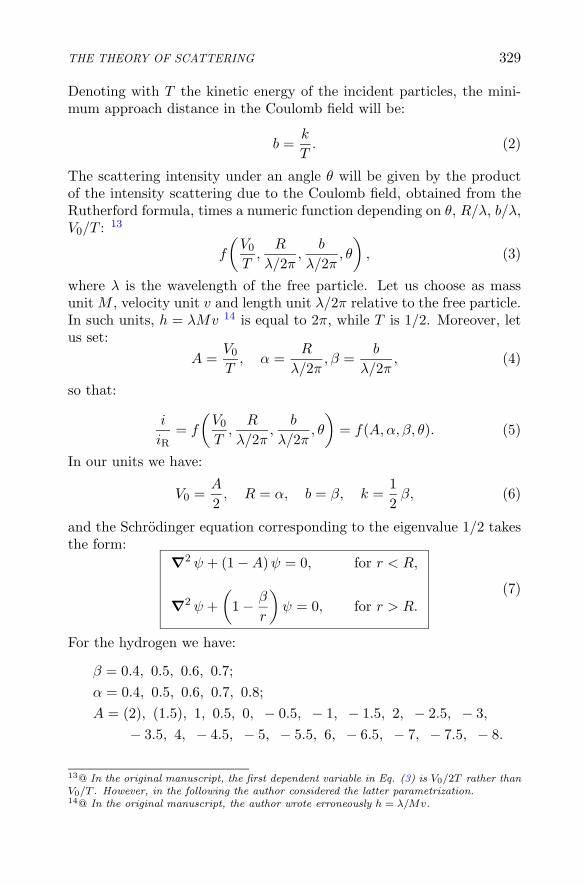
THE THEORY OF SCATTERING 329

Denoting with T the kinetic energy of the incident particles, the mini-mum approach distance in the Coulomb field will be:

b =k

T. (2)

The scattering intensity under an angle θ will be given by the productof the intensity scattering due to the Coulomb field, obtained from theRutherford formula, times a numeric function depending on θ, R/λ, b/λ,V0/T : 13

f

(V0

T,

R

λ/2π,

b

λ/2π, θ

), (3)

where λ is the wavelength of the free particle. Let us choose as massunit M , velocity unit v and length unit λ/2π relative to the free particle.In such units, h = λMv 14 is equal to 2π, while T is 1/2. Moreover, letus set:

A =V0

T, α =

R

λ/2π, β =

b

λ/2π, (4)

so that:

i

iR= f

(V0

T,

R

λ/2π,

b

λ/2π, θ

)= f(A,α, β, θ). (5)

In our units we have:

V0 =A

2, R = α, b = β, k =

12

β, (6)

and the Schrodinger equation corresponding to the eigenvalue 1/2 takesthe form:

∇2 ψ + (1 − A)ψ = 0, for r < R,

∇2 ψ +(

1 − β

r

)ψ = 0, for r > R.

(7)

For the hydrogen we have:

β = 0.4, 0.5, 0.6, 0.7;α = 0.4, 0.5, 0.6, 0.7, 0.8;A = (2), (1.5), 1, 0.5, 0, − 0.5, − 1, − 1.5, 2, − 2.5, − 3,

− 3.5, 4, − 4.5, − 5, − 5.5, 6, − 6.5, − 7, − 7.5, − 8.

13@ In the original manuscript, the first dependent variable in Eq. (3) is V0/2T rather thanV0/T . However, in the following the author considered the latter parametrization.14@ In the original manuscript, the author wrote erroneously h = λ/Mv.

330 E. MAJORANA: RESEARCH NOTES ON THEORETICAL PHYSICS

6.8. TWO-ELECTRON SCATTERING

v, v′ be the velocities of the two beams;

n0, n′0 be the rest number densities of the two beams;

n = n0/√

1 − v2/c2, n′ = n′0/

√1 − v′2/c2 be the number densities

in the laboratory reference frame;

vr be the relative velocity according to the relativistic kinematics;

S(vr) be the cross section.

The number N of collisions for unit volume and time can be written as:

N = a(v, v′

)n n′ = S(vr) n0 n′

0

vr√1 − v2

r/c2.

In terms of a we thus have:

S =a

vr

√1 − v2

r/c2

√1 − v2/c2

√1 − v′2/c2

(classically (that is: non relativistically), we have instead S = a/|v−v′|).Without considering the resonance in the scattering cross section, let u(0 ≤ u ≤ vr) be the velocity of the first electron after the collision in itsinitial reference frame; we have:

dS = S (vr, u) du.

Let us now denote with u1 the relative velocity between the frame ofthe first electron before (after) the collision and that of the second elec-tron after (before) the collision. By taking into account the resonancebetween the two electrons, u and u1 are indistinguishable. Putting, con-ventionally, u ≤ u1, the maximum value of u is given by 15:

umax = umin = c

√√√√1 − 4 (1 − v2

r/c2)(1 +

√1 − v2

r/c2)2 =

y

2

√

2 − y2

c2

(

y = c

√1 −

√1 − v2

r/c2

1 +√

1 + v2r/c2

)

.

The relation between u and u1 is the following:1

√1 − u2/c2

+1

√1 − u2

1/c2= 1 +

1√

1 − v2r/c2

.

15In this case we have u = u1

THE THEORY OF SCATTERING 331

6.9. COMPTON EFFECT

n = n0/√

1 − v2/c2, number of electrons per cm3;

n0, rest number densities of the electron beams;

N , number of photons 16 per cm3;

N0 = Nν0/ν, number of photons per cm3 in the electron frame;

hν, energy of one photon;

hν0, energy of one photon in the electron frame (before or afterthe collision);

u1, relative velocity between the ingoing electron frame and theoutgoing one (according to relativistic kinematics);

S(ν0), cross section.

The number of collisions for unit volume and time is thus:

S(ν0) n0 N0 c = a n N,

so that, in terms of a,

S(ν0) =a

c

1√

1 − v2/c2

ν

ν0.

The differential cross section can be written as:

dS = F (ν0, u) du,

so thatS =

∫ ∞

0F (ν0, u) du.

Classically, the cross section is given by:

Sclass =8π

3e4

m2c4.

16@ For the sake of clarity, here and in the following we have translated with “photons”what was termed “quanta” in the original manuscript.

332 E. MAJORANA: RESEARCH NOTES ON THEORETICAL PHYSICS

6.10. QUASI-STATIONARY STATES

The author considered the transition from a discrete (unperturbed) stateψ0 with energy E0 to a continuum (perturbed) state ψ, assuming thatthe unperturbed system has two continuum spectra φW and ψW withenergy E0 + W . What here reported are the scratch calculations whichprepared the Sect. 28 of Volumetto IV, to which we refer the readerfor notations and further explanations of the arguments treated by theauthor. However, a further generalization is present here with respect towhat considered after Eq. (4.499) of Volumetto IV.

ψ =1

ε2/Q2 + π2Q2

(εI

Q2ψ0 +

ε2|I|2Q4

ψW − ε|I|2Q2

∫ψW ′

W ′ − WdW ′

+ε2IL

Q4φW − εIL

Q4

∫φW ′

W ′ − WdW ′

)

+I

∫e−2πi(ε′−ε)t/hdW ′

(ε′2/Q2 + π2Q2)(W ′ − W )ψ0

+|I|2Q2

∫e−2πi(ε′−ε)t/hε′ψW ′

(ε′2/Q2 + π2Q2)(W ′ − W )dW ′

−|I|2∫

e−2πi(ε′−ε)t/hdW ′

(ε′2/Q2 + π2Q2)(W ′ − W )

∫ψW ′′dW ′′

W ′′ − W ′

+IL

Q2

∫e−2πi(ε′−ε)t/hε′φW ′

(ε′2/Q2 + π2Q2)(W ′ − W )dW ′

−IL

∫e−2πi(ε′−ε)t/hdW ′

(ε′2/Q2 + π2Q2)(W ′ − W )

∫φW ′′dW ′′

W ′′ − W ′

+|L|2Q2

ψW − IL

Q2φW .

ψ =(

A ψ0 + B ψW + CφW +∫

b ψW ′dW ′ +∫

c φW ′dW ′)

e−2πiEt/h,

Quantity A:

1(ε2/Q2 + π2Q2)(ε′ − ε)

=Q2

(ε′ + iπQ2)(ε′ − iπQ2)(ε′ − ε),

R1 = e2πiεt/h e−2π2Q2t/h 12πi(ε + iπQ2)

,

THE THEORY OF SCATTERING 333

R2 =1

ε2/Q2 + π2Q2,

−2πi

(R1 +

12R2

)=

1ε2/Q2 + π2Q2

[e2πiεt e−2π2Q2t/h

×(− ε

Q2+ iπ

)− iπ

],

A =1

ε2/Q2 + π2Q2

[εI

Q2

(1 − e2πiεt/h e−t/2T

)

−Iπi(1 − e(2πi/h)εt e−t/2T

)],

A =I

ε + iπQ2

(1 − e2πiεt/h e−t/2T

).

Quantity B:

1ε2/Q2 + π2Q2

ε2|I|2Q4

+π2|I|2

ε2/Q2 + π2Q2+

|L|2Q2

=1

Q2

(|I|2 + |L|2

)= 1,

B = 1.

Quantity C:

1ε2/Q2 + π2Q2

ε2IL

Q4+

π2IL

ε2/Q2 + π2Q2− IL

Q2= 0,

C = 0.

334 E. MAJORANA: RESEARCH NOTES ON THEORETICAL PHYSICS

Quantity b: 17

∫e−2πi(ε′−ε)t/hdε′

(ε′2/Q2 + π2Q2)(ε′ − ε)(ε′ − ε′′)

=∫

Q2e−2πi(ε′−ε)t/hdε′

(ε′ + iπQ2)(ε′ − iπQ2)(ε′ − ε)(ε′ − ε′′),

−2πi

(R0 +

12R1 +

12R2

),

R0 = e2πiεt/h e−2π2Q2t/h 1−2πi(ε + iπQ2)(ε′′ + ipiQ2)

,

R1 =1

ε2/Q2 + π2Q2

1ε − ε′′

,

R2 = e2πi(ε−ε′′t/h −1ε′′2/Q2 + π2Q2

1ε − ε′′

.

−2πi

(R0 +

12R1 +

12R2

)=

1ε2/Q2 + π2Q2

1ε′′2/Q2 + π2Q2

×[e2πiεt/h e−t/2T

(ε

Q2− iπ

)(ε′′

Q2− iπ

)

−(

ε′′2

Q2+ π2Q2

)πi

ε − ε′′+

(ε2

Q2+ π2Q2

)πie2πi (ε−ε′′)t/h

ε − ε′′

]

,

b = −ε|I|2Q2

1ε′ − ε

1ε2/Q2 + π2Q2

+ε′|I|2Q2

1ε′ − ε

e2πi(ε−ε′)t/h

ε′2/Q2 + π2Q2

+|I|2

ε2/Q2 + π2Q2

1ε′2/Q2 + π2Q2

×[e2πiεt/h e−t/2T

(ε

Q2− iπ

) (ε′

Q2− iπ

)

−(

ε′2

Q2+ π2Q2

)πi

ε − ε′+

(ε2

Q2+ π2Q2

)πie2πi (ε−ε′)t/h

ε − ε′

]

=|I|2

ε + iπQ2

1ε − ε′

− |I|2ε′ + iπQ2

1ε − ε′

e2πi (ε−ε′)t/h

+|I|2 e2πi εt/h−t/2T

(ε + iπQ2)(ε′ + iπQ2),

17@ Cf. the figure above.

THE THEORY OF SCATTERING 335

b =|I|2

(ε + iπQ2)(ε′ + iπQ2)

[−1 + e2πi εt/h−t/2T

+ε + iπQ2

ε − ε′

(1 − e2πi (ε−ε′)t/h

)],

b =|I|2

(ε + iπQ2)(ε′ + iπQ2)

[−e2πi (ε−ε′)t/h + e2πi εt/h−t/2T

+ε′ + iπQ2

ε − ε′

(1 − e2πi (ε−ε′)t/h

)].

Quantity c:

c = −εIL

Q2

1ε′ − ε

1ε2/Q2 + π2Q2

+ε′IL

Q2

1ε′ − ε

e2πi(ε−ε′)t/h

ε′2/Q2 + π2Q2

+IL

ε2/Q2 + π2Q2

1ε′2/Q2 + π2Q2

×[e2πiεt/h e−t/2T

(ε

Q2− iπ

)(ε′

Q2− iπ

)

−(

ε′2

Q2+ π2Q2

)πi

ε − ε′+

(ε2

Q2+ π2Q2

)πie2πi (ε−ε′)t/h

ε − ε′

]

=IL

ε + iπQ2

1ε − ε′

− IL

ε′ + iπQ2

1ε − ε′

e2πi (ε−ε′)t/h

+IL e2πi εt/h−t/2T

(ε + iπQ2)(ε′ + iπQ2).

c =IL

(ε + iπQ2)(ε′ + iπQ2)

[−1 + e2πi εt/h−t/2T

+ε + iπQ2

ε − ε′

(1 − e2πi (ε−ε′)t/h

)].

336 E. MAJORANA: RESEARCH NOTES ON THEORETICAL PHYSICS

ψ = e−2πi Et/h ψW +I

ε + iπQ2

(e−2πiEt/h − e−2πi(E0−k)t/h e−t/2T

)ψ0

− I

ε + iπQ2

∫IψW ′ + LφW ′

ε′ + iπQ2e−2πi Et/h

(1 − e2πi εt/h−t/2T

)dε′

+I

∫IψW ′ + LφW ′

ε′ + iπQ2e−2πi Et/h 1

ε′ − ε

(1 − e2πi(ε−ε′)t/h

)dε′,

ψ = e−2πi Et/h ψW + a e−2πi E0t/h ψ0

+∫

bW

(IψW ′ + LφW ′

)dW ′ · e−2πi E′t/h,

Hψ = E e−2πi Et/hψW + IW e−2πi E0t/hψ0 + aE0e−2πi E0t/hψ0

+∫

a e−2πi E0t/hIW ′ψW ′dW ′ +∫

a e−2πi E0t/hLW ′φW ′dW ′

+∫

E′bW ′(IψW ′ + LφW ′

)e−2πi E′t/hdW ′

+Q2

∫bW ′dW ′ · ψ0 e−2πi E′t/h,

IW = I:

a = − 2πi

h

(e−2πi Wt/hI + Q2

∫bW ′e−2πi W ′t/hdW ′

),

bW ′ = − 2πi

he−2πi W ′t/h a.

ψ = e−2πi Et/hψW

+I

ε + iπQ2

(e−2πiEt/h − e−2πi(E0−k)t/h e−t/2T

)ψ0

− I

ε + iπQ2

∫ (IψW ′ + LφW ′

)

ε′ + iπQ2e−2πi E′t/h

×(1 − e2πi ε′t/h−t/2T

)dε′

+I

ε + iπQ2

∫ (IψW ′ + LφW ′

)

ε − ε′e−2πi Et/h

×(1 − e2πi(ε−ε′)t/h

)dε′.

THE THEORY OF SCATTERING 337

ψ = ψ′ + ψ′′,

ψ′ = e−2πi Et/hψW +I

ε + iπQ2e−2πiEt/h ψ0

− I

ε + iπQ2

∫ (IψW ′ + LφW ′

)

ε′ − εe−2πi Et/h

(1 − e2πi (ε′−ε)t/h

)dε′,

ψ′′ = − I

ε + iπQ2e−2πi(E0−k)t/h e−t/2T ψ0

− I

ε + iπQ2

∫ (IψW ′ + LφW ′

)

ε′ + iπQ2e−2πi E′t/h

(1 − e2πi ε′t/h−t/2T

)dε′.

Appendix:Transforming a differential equation

u′′ +(

δ0 +δ1

r

)u′ +

(ε0 +

ε1r

)u = 0,

χ = rk u.

u = r−k u,

u′ = u

(χ′

χ− k

r

),

u′′ = u

(χ′

χ− k

r

)2

+ u

(χ′′

χ− χ′2

χ2+

k

r2

)

= u

(χ′′

χ− 2

k

r

χ′

χ+

k(k + 1)r2

).

(χ′′

χ− 2

k

r

χ′

χ+

k(k + 1)r2

)+ δ0

χ′

χ− δ0

k

r+

δ1

r

χ′

χ− kδ1

r2+ ε0 +

ε1r

= 0,

χ′′ +(

δ0 +δ1

r− 2

k

r

)χ′ +

(ε0 +

ε1 − kδ0

r+

k(k + 1) − kδ1

r2

)χ = 0.

k =δ1

2; δ1 = 2k,

χ′′ + δ0χ′ +

(ε0 +

ε1 − kδ0

r− k(k − 1)

r2

)χ = 0.

7

NUCLEAR PHYSICS

7.1. WAVE EQUATION FOR THE NEUTRON

Denoting with ε the electric or diamagnetic susceptivity, the Lagrangiandescribing the electromagnetic field is:

−12ε(E2 − H2).

Using Dirac coordinates,

[W

c+ ρ1 σ · p + ρ3 mc +

ε

2cρ3 (E2 − H2)

]ψ = 0.

7.2. RADIOACTIVITY

In the following table the author referred to some radioactive nuclidesgrouped by their atomic number Z. The number following the (old) nameof the given isotope is its mass number. Probably this table was aimedat cataloguing the isotopes existing at the time of Majorana according toZ for further studies.

[1]

Z = 90 U X1 234U Y 231Io 230Rd Ac 227Th 232Rd Th 228

Z = 89 Ac 227Ms Th2 228

1@ In the original manuscript, the unidentified Ref. 9.28 appears here.

339

340 E. MAJORANA: RESEARCH NOTES ON THEORETICAL PHYSICS

Z = 88 Ra 226Ac X 223Ms Th1 228Th X 224

Z = 86 Rn 222An 219Tn 220

Z = 84 Ra A 218Ra C′ 214Ra F 210Ac A 215Ac C′ 211Th A 216Th C′ 212

Z = 83 Ra C 214Ra E 210Ac C 211Th C 212

Z = 82 Ra B 214Ra D 210Ac B 211Th B 212

Z = 81 Ra C′′ 210Ac C′′ 207Th C′′ 208

7.3. NUCLEAR POTENTIAL

In the following pages, the author considered the problem of finding thenucleon potential inside a given nucleus. In particular, he focused on theinteraction between neutrons and protons, assuming that the interactionbetween protons is approximatively given only by the usual electrostaticrepulsion, while that between neutrons is negligible. Many of the resultsdiscussed apply to a general nucleus of atomic number Z and mass num-ber A, although particular attention was here given to α particles.What reported in the following is, at the same time, a preliminary studyand a generalization of what published by Majorana in Z. Phys. 82(1933) 137, or in La Ricerca Scientifica 4 (1933) 559, on the nuclearexchange forces.

7.3.1 Mean Nucleon PotentialSome expressions for the matrix elements of the interaction potentialbetween neutrons and protons in a given nucleus were defined in the fol-lowing. The author considered the case of a nucleus composed of a num-ber a of protons (whose wavefunctions, depending on the coordinates q,were denoted with ψ) and A of neutrons (whose wavefunctions, depend-ing on the coordinates Q, were denoted with ϕ). The state function ofthe nucleons was written as a Slater determinant.With reference to the published papers quoted above, the given form ofthe matrix elements of the interaction potential (also considered in the

NUCLEAR PHYSICS 341

following subsections) in terms of Dirac δ-functions corresponds to thehypothesis that the mean energy per nucleon cannot exceed a certainlimit, whatever large be the nuclear density. It is also assumed that thedensity of neutrons is larger than that of protons.In the second part, it seems that the author considered the particularcase of a nucleus of helium (with only two protons and two neutrons),probably thought as composed of two deuterium nuclei (denoted, in theoriginal manuscript, as d and D, respectively). However, it is also possi-ble that the author was initially studying the scattering of two nuclei withmass numbers a and A, respectively, and that only later on he turnedto the particular case cited above. The interaction potential between thenucleon s in the first nucleus and the nucleon S in the second one wasdenoted with V sS.

ψ1, ψ2, . . . ψa; q1, q2, . . . qa;ϕ1, ϕ2, . . . ϕA; Q1, Q2, . . . QA

(A ≥ a).

ψ =1√a!

∣∣∣∣∣∣

ψ1(q1) . . . ψ1(qa). . .ψa(q1) . . . ψa(qa)

∣∣∣∣∣∣,

ϕ =1√A!

∣∣∣∣∣∣

ϕ1(Q1) . . . ϕ1(QA). . .ϕA(Q1) . . . ϕA(AA)

∣∣∣∣∣∣.

〈q′, Q′|V |q′′, Q′′〉 = δ(q′′ − Q′) δ(Q′′ − q′) f |q′ − Q′|.

〈q′s, Q′s|V sS |q′′s , Q′′

S〉 = δ(q′′s − Q′S) δ(Q′′

S − q′s) f |q′s − Q′S |;

V S =∑

s

V sS , V s =∑

S

V sS ;

V sS =∫∫∫∫

ψ(q′s)ϕ(Q′s)δ(Q

′′S − q′s)

× δ(q′′s − Q′S)ψ(q′′s )ϕ(Q′′

S)dq′sdQ′Sdq′′sdQ′′

S ;

f |q′s − Q′S | =

∫∫f |q′s − q′′s | ψ(q′s)ψ(q′′s )ϕ(q′′s )ϕ(q′s)dq′sdq′′s ;

Vs =

∫∫f |q′s − q′′s | ψ(q′s)ψ(q′′s )

[∑

S

ϕS(q′s)ϕS(q′′s )

]

dq′sdq′′s .

342 E. MAJORANA: RESEARCH NOTES ON THEORETICAL PHYSICS

〈q′|V s|q′′〉 = f |q′ − q′′|∑

S

ϕS(q′)ϕS(q′′).

7.3.2 Computation Of The Interaction Potentialbetween Nucleons

The following calculations seems to be aimed at obtaining an expres-sion for the interaction potential between nucleons (the primed quantitiesprobably refer to neutrons, while the unprimed ones to protons); see alsothe beginning of the next subsection.

∫∫dq dq′

|q − q′|2 =∫

dq

∫dq′

(q − q′)2.

q′ = (ρ, ϑ, ϕ),dq′ = ρ2 sin ϑ dϑ dϕ dρ,

|q − q′|2 = |q2| + ρ2 − 2|q|ρ cos ϑ,

s = |q − q′|,s2 = |ϕ2| + |ρ2| − 2|q|ρ cos ϑ,

� 2s ds = � 2|q|ρ sin ϑ dϑ.

R′ > q:

∫dq′

|q − q′|2 = π

(2R′ +

R′2 − q2

qlog

R′ + q

R′ − q

).

R′ > q:

|q| − ρ ≤ s ≤ |q| + ρ,

dq′ =sρ

|q| dsdϕdρ = 2πsρ

|q|dsdρ.

∫dq′

|q − q′|2 =2π

|q|

∫ρdρ

∫ds

s+ . . . =

2π

|q|

∫ρdρ log

|q| + ρ

|q| − ρ+ . . . .

∫ρ dρ log(q + ρ) =

12ρ2 log(q − ρ) − 1

2

∫ρ2

q + ρdρ

=12ρ2 log(q + ρ) − 1

4(ρ − q)2 − 1

2q2 log(q + ρ).

NUCLEAR PHYSICS 343

∫dq′

|q − q′|2 =2π

q

∫ q

0ρ dρ log

q + ρ

q − ρ+

2π

q

∫ R′

qρ dρ log

ρ + q

ρ − q

=2π

q

{12R′2 log(R′ + q) − 1

4(R′ − q)2

−12q2 log(R′ + q) +

14q2 +

12q2 log q

−[12R′2 log(R′ − q) − 1

4(R′ + q)2

−12q2 log(R′ − q) +

14q2 +

12q2 log q

]}.

dq′ = dx′ dy′ dz′:

F (q) =∫

q′<R′

dq′

|q′ − q|2 =

⎧⎪⎪⎪⎪⎨

⎪⎪⎪⎪⎩

π

(2R′ +

R′2 − q3

qlog

R′ + q

R′ − q

), q < R′;

π

(2R′ − q2 − R′2

qlog

q + R′

q − R′

), q > R′.

1π

F (0) = 4R′,1π

F (R′) = 2R′.

q > R′:

logq + R′

q − R′ = 2(

R′

q+

13

R′3

q3+

15

R′5

q5+ . . .

);

q2 − R′2

q· 2(

R′

q+

13

R′3

q3+ . . .

)= 2R′

(1 − 2

3R′2

q2− 2

15R′4

q4− . . .

).

F (q) + F

(R′2

q

)= 4πR′.

(q > R′) : F (q) =4πR′3

q2

(13

+115

R′2

q2+

135

R′4

q4+ . . .

);

(q < R′) : F (q) = 4πR′(

1 − 13

q2

R′2 − 115

q4

R′4 − 135

q6

R′6 − . . .

).

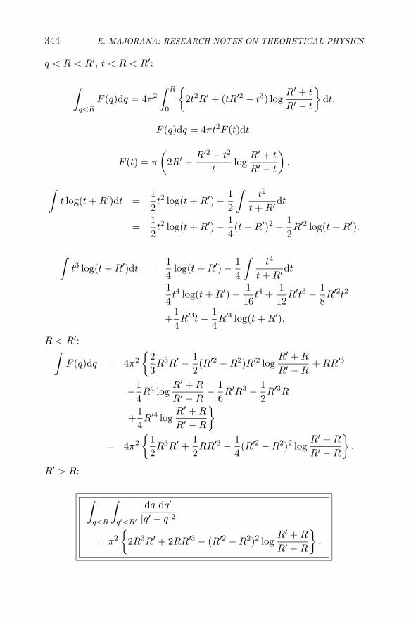
344 E. MAJORANA: RESEARCH NOTES ON THEORETICAL PHYSICS

q < R < R′, t < R < R′:

∫

q<RF (q)dq = 4π2

∫ R

0

{2t2R′ + (tR′2 − t3) log

R′ + t

R′ − t

}dt.

F (q)dq = 4πt2F (t)dt.

F (t) = π

(2R′ +

R′2 − t2

tlog

R′ + t

R′ − t

).

∫t log(t + R′)dt =

12t2 log(t + R′) − 1

2

∫t2

t + R′dt

=12t2 log(t + R′) − 1

4(t − R′)2 − 1

2R′2 log(t + R′).

∫t3 log(t + R′)dt =

14

log(t + R′) − 14

∫t4

t + R′dt

=14t4 log(t + R′) − 1

16t4 +

112

R′t3 − 18R′2t2

+14R′3t − 1

4R′4 log(t + R′).

R < R′:∫

F (q)dq = 4π2

{23R3R′ − 1

2(R′2 − R2)R′2 log

R′ + R

R′ − R+ RR′3

−14R4 log

R′ + R

R′ − R− 1

6R′R3 − 1

2R′3R

+14R′4 log

R′ + R

R′ − R

}

= 4π2

{12R3R′ +

12RR′3 − 1

4(R′2 − R2)2 log

R′ + R

R′ − R

}.

R′ > R:

∫

q<R

∫

q′<R′

dq dq′

|q′ − q|2

= π2

{2R3R′ + 2RR′3 − (R′2 − R2)2 log

R′ + R

R′ − R

}.

NUCLEAR PHYSICS 345

7.3.3 Nucleon DensityIn the following the author worked out some expressions for the nucleondensity, starting from the potential and kinetic energy densities V andT of a system of nucleons (the proton and neutron density are denotedwith ρ(=

∑Z1 ψiψ1) and ρ′(=

∑Y1 ϕiϕ1), respectively). Notice that the

potential energy density V is given, up to a factor −π2, by the last for-mula in the previous subsection, with the replacements R,R′ → ρ, ρ′.

Potential energy per unit volume:

−V = 2ρρ′13 + 2ρ′ρ

13 − (ρ′

23 − ρ

23 )2 log

ρ′13 + ρ

13

|ρ′ 13 − ρ13 |

.

Kinetic energy per unit volume:

T =35(ρ

53 + ρ′

53 ).

ρ = ρ′: 2

−V = 4ρ43 =

250081

,

T =65ρ

53 =

125081

.

T = −12V.

65ρ

53 = ρ

43 , ρ

13 =

106

=53, ρ =

12527

;

−V

ρ=

203

,

T

2ρ=

53.

−∂V

∂ρ= −∂V

∂ρ′=

83ρ

13 =

409

,

∂T

∂ρ=

∂T

∂ρ′= ρ

23 =

259

;

2@ The numerical values 2500/81 and 1250/81 seem to have been written by the author afterhe deduced the numerical value for ρ (see below).

346 E. MAJORANA: RESEARCH NOTES ON THEORETICAL PHYSICS

−(

∂V

∂ρ+

∂T

∂ρ

)=

53.

ρ �= ρ′ (ρ < ρ′):

−∂V

∂ρ= 2ρ′

13 +

23ρ−

23 ρ′ +

43ρ−

13

(ρ′

23 − ρ

23

)log

ρ′13 + ρ

13

ρ′13 − ρ−

13

−13ρ−

23

(ρ′

23 − ρ

23

)(ρ′

13 + ρ

13 ) · log

(ρ′

13 + ρ

13

),

−∂V

∂ρ′= 2ρ

13 +

23ρ′−

23 ρ − 4

3ρ′−

13

(ρ′

23 − ρ

23

)log

ρ′13 + ρ

13

ρ′13 − ρ−

13

+13ρ′−

23

(ρ′

23 − ρ

23

)(ρ′

13 + ρ

13

)· log(ρ′

13 + ρ

13

);

∂T

∂ρ= ρ

23 ,

∂T

∂ρ′= ρ′

23 .

T = −12V :

35(ρ

53 + ρ′

53 ) = ρρ′

13 + ρ′ρ

13 − 1

2(ρ′

23 − ρ

23 )2 log

ρ′13 + ρ

13

ρ′13 − ρ

13

.

ρ′ = kρ:

35ρ

53 (1 + k

53 ) = (k + k

13 )ρ

43 − 1

2ρ

43 (k

23 − 1)2 log

k13 + 1

k13 − 1

,

35ρ

13 (1 + k

53 ) = (k + k

13 ) − 1

2(k

23 − 1)2 log

k13 + 1

k13 − 1

.

[3]

ρ =12527

⎧⎪⎨

⎪⎩

k13 + k − 1

2(k23 − 1)2 log k

13 +1

k13 −1

1 + k53

⎫⎪⎬

⎪⎭

3

.

3@ In the original manuscript, the power 2 of the factor (k23 − 1) in the following equation

is missing.

NUCLEAR PHYSICS 347

7.3.4 Nucleon Interaction IExplicit expressions for a particular form of the interaction potentialbetween Z protons and Y neutrons are worked out. See also the paperpublished by Majorana in Z. Phys. 82 (1933) 137, or in La RicercaScientifica 4 (1933) 559.

Denote with q, Q the center-of-mass coordinates.

〈q′Q′|V |quQu〉 = −δ(q′′ − Q′) δ(Q′′ − q′)λe2

r.

N = Z + Y .1

(Z/2)!

∑ψ1(q1) . . . ψZ/2(qZ/2)ψ1(qZ/2+1) . . . ψZ/2(qZ),

1(Y/2)!

∑ϕ1(Q1) . . . ϕY/2(qY/2)ϕ1(QY/2+1) . . . ϕY/2(QY ).

U = −Z∑

i=1

Y∑

�=1

∫ψi(q

′)ψi(q′′)ϕ�(q′′)ϕ�(q′)

λe2

|q′ − q′′|dq′dq′′

+Z∑

i<k=2

∫ψi(q

2)ψi(q′′)ψk(q′′)ψk(q′′)

e2

|q′ − q′′| dq′dq′′

+ negligible exchange terms.

[4]

ρ =Z∑

1

ψiψi, ρ′ =Y∑

1

ϕiϕi.

U = −∫〈q′′|ρ|q′〉 〈q′|ρ′|q′′〉 λe2

|q′ − q′′| dq′dq′′

+12

∫〈q′|ρ|q′〉 〈q′′|ρ|q′′〉 e2

|q′ − q′′| dq′dq′′.

〈q′|VP |q′′〉 = − λe2

|q′ − q′′| 〈q′|ρ′|q′′〉

+ δ(q′ − q′′)∫〈q′′′|ρ|q′′′〉 e2

|q′ − q′′′| dq′′′,

〈Q′|VN |Q′′〉 = − λe2

|Q′ − Q′′| 〈Q′|ρ|Q′′〉.

4@ Notice that here the author refers to the “ordinary” exchange energy depending on theelectrostatic interaction among protons.

348 E. MAJORANA: RESEARCH NOTES ON THEORETICAL PHYSICS

[5]

Aq− v2,q+ v

2=

1h3

∫e−2πi p·v/hA(p, q) dp,

A(p, q) =∫

e2πi p·v/hAq− v2,q+ v

2dv.

In Classical Mechanics: 6

ρ =

⎧⎨

⎩

2, p < P,

0, p > P ;ρ′ =

⎧⎨

⎩

2, p′ < P ′,

0, p′ > P ′.

VP (p, q) =1h3

∫e2

|q′ − q| ρ(q′, p′) dq′dp′ − 1h

∫λe2

π|p − p′|2 ρ′(Q, p′) dp′,

VN = −1h

∫λe2

π|p − p′|2 ρ(q, p) dp.

P = P (q), P ′ = P ′(Q);∫

p<Pdp =

43πP 3,

∫

p′<P ′dp′ =

43πP ′3.

VP (p, q) =∫

8π

3e2

|q′ − q|P 3

h3dq′

−2λe2

h

(2P ′ +

P ′2 − p2

plog

P ′ + p

P ′ − p

)p < P ′,

VP (p, q) =∫

8π

3e2

|q′ − q|P 3(q′)

h3dq′

−2λe2

h

(2P ′(q) − p2 − P ′2

plog

p + P ′

p − P ′

)p > P ′.

5@ In the following, the author deals with a semiclassical approach, which is valid when thenumber of particles is sufficiently large. The quantities VP and VN considered below are,then, the classical functions corresponding to the quantum matrix elements discussed before.See E. Majorana, Z. Phys. 82 (1933) 137 or La Ricerca Scientifica 4 (1933) 559.6@ In the following, the author postulates for simplicity that the one-particle states are eitherempty or doubly occupied with opposite spins. Moreover, by assuming that at a given positionq (or Q) the protons (or neutrons) occupy the states with minimum kinetic energy, it followsthat a maximum value P for the proton momentum (and, similarly, P ′ for neutrons) doesexist. See the papers quoted in the previous footnote.

NUCLEAR PHYSICS 349

[7]

VN (p, q) = −2λe2

h

(2P +

P 2 − p2

Plog

P + p

P − p

), p < P ;

VN (p, q) = −2λe2

h

(2P − p2 − P 2

Plog

p + P

p − P

), p > P.

C(q) =∫

8π

3P 3(q′)|q′ − q|

e2

h3dq′.

VP (P, q) =

⎧⎪⎪⎪⎪⎨

⎪⎪⎪⎪⎩

C − 2λe2

h

(2P ′ +

P ′2 − P 2

Plog

P ′ + P

P ′ − P

), P < P ′;

C − 2λe2

h

(2P ′ − P 2 − P ′2

Plog

P + P ′

P − P ′

), P > P ′;

VN (P ′, q) =

⎧⎪⎪⎪⎪⎨

⎪⎪⎪⎪⎩

−2λe2

h

(2P − P ′2 − P 2

P ′ logP ′ + P

P ′ − P

), P < P ′;

−2λe2

h

(2P − P 2 − P ′2

P ′ logP + P ′

P − P ′

), P > P ′.

T =P 2

2M.

7@ The original manuscript presents here an insert dealing with the following Fourier trans-forms:

ϕ(ξ) =

Z

e−2πiξxf(x)dx, f(x) =

Z

e2πiξxϕ(ξ)dξ,

ϕ′(ξ) =

Z

e−2πiξxf ′(x)dx, f ′(x) =

Z

e2πiξxϕ′(ξ)dξ,

where, in particular:

ϕ′(ξ) =1

ξϕ(ξ), f ′(x) =

Z

1

π(x − x1)2f(x1)dx1.

350 E. MAJORANA: RESEARCH NOTES ON THEORETICAL PHYSICS

[8]

VP (P, q) +P 2

2M= −AP ,

VN (P ′, q) +P ′2

2M= −AN .

By considering a statistical method: 9

TP (q) =3P 2

10M,

V P (q) = C − 2λe2

h

[32P ′ +

32

P ′3

P 2− 3

4(P ′2 − P 2)2

P 3log

P ′ + P

|P ′ − P |

],

TN (q) =3P ′2

10M,

V N (q) = −2λe2

h

[32P +

32

P 3

P ′2 − 34

(P ′2 − P 2)2

P ′3 logP ′ + P

|P ′ − P |

];

P 3(V P − C) = P ′3 V N .

Limiting condition:

−{

P 3

P 3 + P ′3[V P (Q) + TP (Q)

]+

P ′3

P 3 + P ′3[TN (Q)

]}

=P 3

P 3 + P ′3 AP +P ′3

P 3 + P ′3 AN .

8@ In the following, the author probably denotes with AP (or AN ) the energy associatedwith the proton (or neutron) exchange interaction.9@ An application of the theory of nuclear forces introduced above to heavy nuclei, composedof a large number of nucleons, is now apparently investigated, so that statistical methodsmay apply.

NUCLEAR PHYSICS 351

7.3.4.1 Zeroth approximation.C = 0; P = constant, P ′ = constant.k = P ′/P :

VP (P, q) = −2λe2

hP

[2k + (k2 − 1) log

k + 1|k − 1|

],

VN (P ′, q) = −2λe2

hP

[2 − k2 − 1

klog

k + 1|k − 1|

].

TP =3P 2

10M,

V N = −2λe2

hP

[32k +

32k3 − 3

4(k2 − 1)2 log

k + 1|k − 1|

],

TN =3k2P 2

10M,

V P = −2λe2

hP

[32

+3

2k3− 3

4(k2 − 1)2

k3log

k + 1|k − 1|

].

Particular case: k = 1.

VP (P, q) = VN (P ′, q) = −4λe2

hP, T =

P 2

2M;

V N (q) = −6λe2

hP = V P (q), TN =

3P 2

10M.

−3λe2

hP +

3P 2

10M= −4λe2

hP +

P 2

2M,

λe2

hP =

P 2

5M,

P = 5Mλe2

h.

VP (P, q) = −20Mλ2e4

h2, Tnuc =

252

Mλ2e4

h2;

V = −30Mλ2e4

h2, T =

152

Mλ2e4

h2.

352 E. MAJORANA: RESEARCH NOTES ON THEORETICAL PHYSICS

AP = AN =152

λ2Me4

h2.

[10]

7.3.5 Nucleon Interaction IIExplicit expressions for another particular form of the interaction poten-tial between Z protons and Y neutrons are worked out.

〈q′, Q′|V |q′′, Q′′〉 = −δ(q′′ − Q′)δ(Q′′ − q′)A e−|q′−q′′|/ε.

For protons: ρ =∑Z

1 ψiψi; for neutrons: ρ′ =∑Y

1 ϕiϕi.

〈q′|VP |q′′〉 = −A e−|q′−q′′|/ε〈q′|ρ′|q′〉 + δ(q′ − q′′)∫

e2

|q − q′| 〈q|ρ|q〉 dq,

〈q′|VN |q′′〉 = −A e−|q′−q′′|/ε〈q′|ρ|q′′〉.

In Classical Mechanics11, assuming a degenerate gas of nucleons:

ρ =

⎧⎨

⎩

2, p < P,

0, p > P ;ρ′ =

⎧⎨

⎩

2, p < P ′,

0, p > P ′.

A e−|q′−q′′|/ε = A e−v/ε = A e−(h/ε)(v/h) = A e−k v/h, (k = h/ε).

VP (p, q) =1h3

∫e2

|q − q′|ρ(q′, p′) dq′dp′

−A

∫8πh/ε

(h2/ε2 + 4π2|p − p′|2)2ρ′(q, p′) dp′,

VN (p, q) = −A

∫8πh/ε

(h2/ε2 + 4π2|p − p′|2)2ρ(q, p′) dp′.

10@ In the original manuscript there appears also the following note:

15

2

Me4

h2= 9500 V

(V stands for eV), where the nucleon mass value M � 938 MeV had been used.11@ See footnote 6.

NUCLEAR PHYSICS 353

Let us set:

P0 =h

2πε,

h

ε= 2πP0.

[12]

VP (p, q) =1h3

∫e2

|q − q′|ρ(q′, p′) dq′dp′

− A

π2

∫P0

(P 20 + |p − p′|2)2 ρ′(q, p′) dp′,

VN (p, q) = − A

π2

∫P0

(P 20 + |p − p′|2)2 ρ′(q, p′) dp′.

P = P (q), P ′ = P ′(q),∫p<P dp = 4πP 3/3.

For a degenerate gas of nucleons:

VP (p, q) =8π

31h3

∫e2

|q − q′|P3(q′) dq′ − 2A

π2

∫

p′<P

P0

(P 20 + |p − p′|2)2 dp′,

VN (p, q) = −2A

π2

∫

p′<P

P0

(P 20 + |p − p′|2)2 dp′.

VP (p, q) =∫

8π

3e2

|q′ − q|P 3(q′)

h3dq′ − 2A

π

{arctan

P ′ + p

P0

+arctanP ′ − p

P0− 1

2P0

plog

P 20 + (P ′ + p)2

P 20 + (P ′ − p)2

},

VN (p, q) = −2A

π

{arctan

P + p

P0+ arctan

P − p

P0

−12

P0

plog

P 20 + (P + p)2

P 20 + (P − p)2

}.

12@ In the original manuscript, the unidentified Ref. 5.25 appears here.

354 E. MAJORANA: RESEARCH NOTES ON THEORETICAL PHYSICS

[13]

VP (P, q) +P 2

2M= −AP ,

VN (P ′, q) +P 2

2M= −AN .

VP (P, q) =∫

8π

3e2

|q′ − q|P 3(q′)

h3dq′ − 2A

π

{arctan

P ′ + P

P0

+arctanP ′ − P

P0− 1

2P0

plog

P 20 + (P ′ + P )2

P 20 + (P ′ − P )2

},

VN (P ′, q) = −2A

π

{arctan

P + P ′

P0+ arctan

P − P ′

P0

−12

P0

P ′ logP 2

0 + (P + P ′)2

P 20 + (P − P ′)2

}.

Limiting conditions:

−[P 3V P (Q) + P 3TP (Q) + P ′3TN (Q)

]= P 3AP + P ′3AN ;

P 3V P = P ′3VN + P 3C,

P 3(V P − C

)= P ′3V N .

C = C =∫

8π

3e2

|q − q′|P 3(q′)

h3dq′.

13@ In the original manuscript, the unidentified Ref. 11.59 appears here.

NUCLEAR PHYSICS 355

P ′3V N = −2A

π

{P0PP ′ + (P 3 + P ′3) arctan

P + P ′

P0

−(P ′3 − P 3) arctanP ′ − P

P0

−P03(P 2 + P ′2) + P 2

0

4log

P 20 + (P + P ′)2

P 20 + (P ′ − P )2

}

= P 3(V p − C).

7.3.5.1 Evaluation of some integrals.For p < P ′:[14]

∫

p′<P ′

P0

(P 20 + |p − p′|2)2 dp′ =

=2πP0

P

[∫ p

0s ds

∫ p+s

p−s

t dt

(P 20 + t2)2

+∫ P ′

ps ds

∫ s+p

s−p

t dt

(P 20 + t2)2

]

=2πP0

p

[∫ p

0s ds · 1

2

{1

P 20 + (p − s)2

− 1P 2

0 + (p + s)2

}

+∫ P ′

ps ds · 1

2

{1

P 20 + (s − p)2

− 1P 2

0 + (s + p)2

}]

=2πP0

p

∫ P ′

0s ds · 1

2

{1

P 20 + (p − s)2

− 1P 2

0 + (p + s)2

}

(the last expression holds also for p > P ′).

∫s ds

P 20 + (p − s)2

=∫

(p − s) d(p − s)P 2

0 + (p − s)2+∫

p ds

P 20 + (p − s)2

=12

log[P 2

0 + (p − s)2]+

p

P0arctan

s − p

P0,

14@ In the original manuscript, the unidentified Ref. 2.50 appears here.

356 E. MAJORANA: RESEARCH NOTES ON THEORETICAL PHYSICS

∫s ds

P 20 + (p + s)2

=12

log[P 2

0 + (p + s)2]− p

P0arctan

p + s

P0;

∫ P ′

0

s ds

P 20 + (p − s)2

=12

logP 2

0 + (P ′ − p)2

P 20 + p2

+p

P0

(arctan

P ′ − p

P0+ arctan

p

P0

),

∫ P ′

0

s ds

P 20 + (p + s)2

=12

logP 2

0 + (P ′ + p)2

P 20 + p2

− p

P0

(arctan

P ′ − p

P0− arctan

p

P0

).

∫

p′<P ′

P0

(P 20 + (p − p′)2)2

dp′ = π

{−1

2P0

plog

P 20 + (P ′ + p)2

P 20 + (P ′ − p)2

+arctanP ′ + p

P0+ arctan

P ′ − p

P0

}.

[15]∫

p<Pdp

∫

p′<P ′

P0

(P 20 + |p − p′2|2)2 dp′ = 4π3

{∫ P

0p2 arctan

P ′ + p

P0dp

+∫ P

0p2 arctan

P ′ − p

P0dp − 1

2P0

∫ P

0p log

P 20 + (P ′ + p)2

P 20 + (P ′ − p)2

dp

}.

∫p2 arctan

P ′ + p

P0dp

=13

p3 arctanP ′ + p

P0− 1

3P0

∫p3

P 20 + (P ′ + p)2

dp

=13

p3 arctanP ′ + p

P0

−13P0

∫(p + P ′)3 − 3P ′(p + P ′)2 + 3P ′2(p + P ′) + P ′3

P 20 + (p + P ′)2

dp

15@ In the original manuscript, the unidentified Ref. 3.43 appears here.

NUCLEAR PHYSICS 357

=13

p3 arctanp + P ′

P0− 1

3P0

[∫(p + P ′) dp −

∫3P ′ dp

+∫

(3P ′2 − P 20 )(p + P ′)

P 20 + (p + P ′)2

dp −∫

P ′(P ′2 − 3P 20 )

P 20 + (p + P ′)2

dp

]

=13

p3 arctanp + P ′

P0− 1

3P0

[12p2 − 2P ′p

+3P ′2 − P 2

0

2log{P 2

0 + (p + P ′)2}− P ′(P ′2 − 3P 2

0 )P0

arctanp + P ′

P0

].

∫p2 arctan

P ′ − p

P0=

13

p3 arctanP ′ − p

P0+

13

P0

[12p2 + 2P ′p

+3P ′2 − P 2

0

2log{P 2

0 + (p − P ′)2}− P ′(P ′3 − 3P 2

0 )2

P0arctan

P ′ − p

P0

].

∫p log

P 20 + (p + P ′)2

P 20 + (p − P ′)2

dp

=12

p2 logP 2

0 + (p + P ′)2

P 20 + (p − P ′)2

−∫

p2(p + P ′)P 2

0 + (p + P ′)2dp

+∫

p2(p − P ′)P 2

0 + (p − P ′)2dp

=12

p2 logP 2

0 + (p + P ′)2

P 20 + (p − P ′)2

−∫

(p + P ′)3 − 2P ′(p + P ′)2 + P ′2(p + P ′)P 2

0 + (p + P ′)2dp

+∫

(p − P ′)3 + 2P ′(p − P ′)2 + P ′2(p − P ′)P 2

0 + (p − P ′)2dp

=12

p2 logP 2

0 + (p + P ′)2

P 20 + (p − P ′)2

−∫

(p + P ′) dp +∫

2P ′dp

−∫

(P ′2 − P 20 )(p + P ′)

P 20 + (p + P ′)2

dp +∫

2P ′P 20 dp

P 21 + (p + P ′)2

+∫

(p − P ′) dp +∫

2P ′dp +∫

(P ′2 − P 20 )(p − P ′)

P 20 + (p − P ′)2

dp

358 E. MAJORANA: RESEARCH NOTES ON THEORETICAL PHYSICS

−∫

2P ′P 20

P 20 + (p − P ′)2

dp

=

12

p2 logP 2

0 + (p + P ′)2

P 20 + (p − P ′)2

+ 2P ′p − P ′2 − P 20

2log

P 20 + (p + P ′)2

P 20 + (p − P ′)2

−2P ′P0 arctanP ′ + p

P0+ 2P ′P0 arctan

P ′ − p

P0.

∫p2 arctan

P ′ + p

P0dp +

∫p2 arctan

P ′ − p

P0dp

−12P0

∫p log

P 20 + (p + P ′)2

P 20 + (p − P ′)2

dp

=13P0P

′p +13(p3 + P ′3) arctan

P ′ + p

P0+

13(p3 − P ′3) arctan

P ′ − p

P0

−3P0P2 + 3P0P

′2 + P 30

12log

P 20 + (p + P )2

P 20 + (p − P )2

.

∫

p<P

∫

p′<P ′

P0 dp dp′

(P 2 + |p − p′|2)2

=43π2

{P0PP ′ + (P 3 + P ′3) arctan

P + P ′

P0

− (P ′3 − P 3) arctanP ′ − P

P0

−3P0P′2 + P 3

0 + 3P0P′2

4log

P 20 + (P + P ′)2

P 20 + (P ′ − P )2

}.

7.3.5.2 Zeroth approximation.C = 0; P 3V P = P ′3V N ;P = constant, P ′ = constant.k = P ′/P , t = Po/P :

NUCLEAR PHYSICS 359

TP (P, q) =P 2

2M,

TN (P ′, q) =P ′2

2M=

k2P 2

2M.

VP (P, q) = −2A

π

{arctan

1 + k

t+ arctan

k − 1t

− t

2log

(k + 1)2 + t2

(k − 1)2 + t2

},

VN (P ′, q) = −2A

π

{arctan

1 + k

t− arctan

k − 1t

− t

2klog

(k + 1)2 + t2

(k − 1)2 + t2

}.

P 3V P = −2A

πP 3

{kt + (1 + k3) arctan

1 + k

t

−(k3 − 1) arctank − 1

t

−t3(1 + k2) + t2

4log

(k + 1)2 + t2

(k − 1)2 + t2

}.

Particular case: k = 1, P = P ′.

VP (P, q) = VN (P ′, q) = −2A

π

{arctan

2t− t

2log

4 + t2

t2

};

V P = −2A

π

{t + 2 arctan

2t− t

6 + t2

4log

4 + t2

t2

}.

+2A

π

{t + 2 arctan

2t− t

6 + t2

4log

4 + t2

t2

}− 3P 2

5M

=2A

π

{arctan

2t− t

2log

4 + t2

t2

}− P 2

M.

360 E. MAJORANA: RESEARCH NOTES ON THEORETICAL PHYSICS

[16]

2P 2

5M=

2A

π

{t

2 + t2

4log

4 + t2

t2− t

},

P 2

2M=

5A

2π

{t

2 + t2

4log

4 + t2

t2− t

}.

P 2

2M= Ay;

P 20

2M= Ax;

P0

P= t =

√x

y;

y =52π

{√x

y

[x + 2y

4ylog

x + 4y

x− 1]}

.

y =52π

{t

2 + t2

4log

4 + t2

t2− t

}.

T =35T (P ); P0 =

h

2πε.

[17]t =√

x/y x = T (P0)/A y = T (P )/A −V (P )/A0.3 0.0213 0.237 0.5400.4 0.0387 0.242 0.4590.5 0.0587 0.235 0.3940.6 0.0806 0.224 0.3390.7 0.1039 0.212 0.2930.8 0.1261 0.197 0.253

t =√

x/y T/A −V /A [−V (P ) − T (P )]/A [−V /2 − T ]/A0.3 0.142 0.892 0.303 0.3040.4 0.145 0.724 0.217 0.2170.5 0.141 0.600 0.159 0.1590.6 0.134 0.498 0.115 0.1150.7 0.127 0.417 0.081 0.08150.8 0.118 0.349 0.056 0.0565

16@ In the original manuscript, the unidentified Ref. 1.03 appears here.17@ The numerical values in the following tables have been obtained by using the appropriateequations above, with a given value of the parameter t. In particular, x has been calculatedfrom x = t2y. Note that, sometimes, the last digit in the numerical values appearing in thetable is slightly erroneous.

NUCLEAR PHYSICS 361

For t = 0.6:

A = 80 · 106 V;

T (P0) = 6.5 · 106 V;

2πε = 11 · 10−13, ε = 1.75 · 10−13;

−V (P ) = 27 · 106 V;

T (P ) = 18 · 106 V;

−V (P ) − T (P ) = 9 · 106 V;

−V = 40 · 106 V;

T = 11 · 106 V;

−V /2 − T = 9 · 106 V.

V (0, q) =2A

π

(2 arctan

1t− 2t

1 + t2

).

t −V (0, q)/A0.3 1.2800.4 1.0760.5 0.9000.6 0.7500.7 0.6240.8 0.519

——————–

General case: k > 1, k = P ′/P , t = P0/P .

V P = k3V N = −2A

π

{kt + (1 + k3) arctan

1 + k

t

−(k3 − 1) arctank − 1

t− t

3(1 + k2) + t2

4log

(k + 1)2 + t2

(k − 1)2 + t2

}.

AP = −VP (P ) − TP (P )

=2A

π

{arctan

1 + k

t+ arctan

k − 1t

− t

2log

(k + 1)2 + t2

(k − 1)2 + t2

}− P 2

2M,

362 E. MAJORANA: RESEARCH NOTES ON THEORETICAL PHYSICS

AN = −VN (P ′) − TN (P ′)

=2A

π

{arctan

1 + k

t− arctan

k − 1t

− t

2klog

(k + 1)2 + t2

(k − 1)2 + t2

}− k2P 2

2M.

TP =3P 2

10M; TN =

3k2P 2

10M.

−V P − TP − k3TN = AP + k3AN .

P 2

2M+

k5P 2

2M− 3P 2

10M− 3k5P 2

10M

=2A

π

{1 + k2 + t2

4log

(k + 1)2 + t2

(k − 1)2 + t2− kt

}=

1 + k5

5MP 2,

P 2

2M=

51 + k5

A

πt

{1 + k2 + t2

4log

(k + 1)2 + t2

(k − 1)2 + t2− k

}.

y =1A

P 2

2M; x =

1A

P 20

2M;

t =P0

P=√

x

y=

√T (P0)T (P )

; T (P0) = t2T (P ).

y =5

1 + k5

t

π

{1 + k2 + t2

4log

(k + 1)2 + t2

(k − 1)2 + t2− k

}.

y = T (P )/A:

k = 1 k = 21/19 k = 22/18 k = 23/17t = 0.5 0.235 0.204 0.157 0.109

0.6 0.225 0.196 0.154 0.1110.7 0.211 0.187 0.149 0.1090.8 0.195 0.174 0.142 0.1060.9 0.179 0.162 0.133 0.1011.0 0.165 0.194 0.124 0.096

NUCLEAR PHYSICS 363

k2y = T (P ′)/A:

k = 1 k = 21/19 k = 22/18 k = 23/17t = 0.5 0.236 0.249 0.234 0.199

0.6 0.225 0.240 0.231 0.2020.7 0.211 0.228 0.223 0.2000.8 0.195 0.213 0.212 0.1940.9 0.179 0.198 0.199 0.1851.0 0.165 0.182 0.186 0.175

7.3.6 Simple Nuclei IIn the following pages the author considered the nucleon interaction dis-cussed in Sect. 7.3.4.

b0 =h2

4π2Me2= 2.9 · 10−12 = a0

m

M,

S =2π2Me4

h2=

M

m· 1 Rh = 25000 V,

e2

b0= 50000 V.

For deuterium 2H:

q = q1 − q2, ψ0 = e−λx/2b0 , E0 = −λ2

2S.

For Z + Y = N > 2:

ψ ∼ ψ1(q1)ψ2(q2) . . . ψn(qn),

withq1 + q2 + . . . + qn = 0.

Q =1n

(q1 + q2 + . . . + qn).

ψ = ψ(q1 − Q, q2 − Q, q3 − Q, . . . , qn − Q),

q′ = q1 − Q, q′2 = q2 − Q, . . . q′n = qn − Q.

q′1 + q′2 + . . . + q′n = 0;

364 E. MAJORANA: RESEARCH NOTES ON THEORETICAL PHYSICS

ψ = ψ(q′1, q′2, . . . , q′n).

p′i =h

2πi

∂

∂qi; p′i =

h

2πi

∂

∂qi.

p1 = p′1 −1n

(p′1 + p′2 + . . . + p′n),. . .

pi = p′i −1n

(p′1 + p′2 + . . . + p′n);

pi = p′1 −1n

∑pi.

∑p2

i =∑

p′2i − 2n

(∑p′i

)2+

1n

(∑p′i

)2=∑

p′2i − 1n

(∑p′i

)2.

T =1

2M

{∑p′2i − 1

n

(∑pi

)}.

For an α particle:

ψ ∼ e−s(r1+r2+r3+r4)/b0 ,

r1 = |q1|, r2 = |q2|, r3 = |q3|, r4 = |q4|.

∑p′2i ψ = − h2

4π2

(4s2

b20

− 2r1

s

b0− 2

r2

s

b0− 2

r3

s

b0− 2

r4

s

b0

)ψ;

pi = (x1i , x

2i , x

3i ),

∑p′iψ = − s

b0

42πi

(xk

1

r1+

xk2

r2+

xk3

r3+

xk4

r4

)ψ;

(∑p′i

)2ψ =

{

− h2

4π2

s2

b20

(

4 + 2∑

i<k

qi · qk

rirk

)

+s

b0

h2

4π2

(2r1

+2r2

+2r3

+2r4

)}ψ.

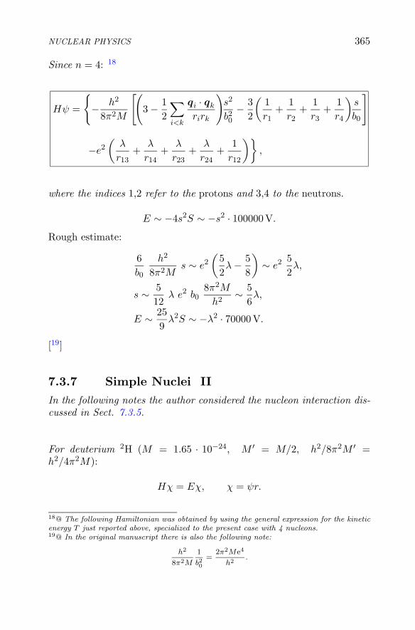
NUCLEAR PHYSICS 365

Since n = 4: 18

Hψ =

{

− h2

8π2M

[(

3 − 12

∑

i<k

qi · qk

rirk

)s2

b20

− 32

(1r1

+1r2

+1r3

+1r4

)s

b0

]

−e2

(λ

r13+

λ

r14+

λ

r23+

λ

r24+

1r12

)},

where the indices 1,2 refer to the protons and 3,4 to the neutrons.

E ∼ −4s2S ∼ −s2 · 100000 V.

Rough estimate:

6b0

h2

8π2Ms ∼ e2

(52λ − 5

8

)∼ e2 5

2λ,

s ∼ 512

λ e2 b08π2M

h2∼ 5

6λ,

E ∼ 259

λ2S ∼ −λ2 · 70000 V.

[19]

7.3.7 Simple Nuclei IIIn the following notes the author considered the nucleon interaction dis-cussed in Sect. 7.3.5.

For deuterium 2H (M = 1.65 · 10−24, M ′ = M/2, h2/8π2M ′ =h2/4π2M):

Hχ = Eχ, χ = ψr.

18@ The following Hamiltonian was obtained by using the general expression for the kineticenergy T just reported above, specialized to the present case with 4 nucleons.19@ In the original manuscript there is also the following note:

h2

8π2M

1

b20=

2π2Me4

h2.

366 E. MAJORANA: RESEARCH NOTES ON THEORETICAL PHYSICS

H = −(

h2

4π2M

∂

∂r2+ A e−r/ε

).

χ ∼ r

(1 +

r

ξ

)e−r/η.

∫χ2dr =

∫r2e−2r/ηdr +

2ξ

∫r3e−2r/ηdr +

1ξ2

∫r4e−2r/ηdr

=η3

4+

3η4

4ξ+

3η5

4ξ2=

η3

4

(1 + 3

η

ξ+

η2

ξ2

).

∂χ

∂r=[1 +(

2ξ− 1

η

)r − 1

ξηr2

]e−r/η,

∂2χ

∂r2=[(

2ξ− 2

η

)−(

4ξη

− 1η2

)r +

1ξη2

r2

]e−r/η.

−Hχ =h2

4π2M

[(2ξ− 2

η

)−(

4ξη

− 1η2

)r +

1ξη2

r2

]e−r/η

+A e−(1/ε+1/η)r · r(

1 +r

ξ

).

−χHχ =h2

4π2M

[(2ξ− 2

η

)r +(

2ξ2

− 6ξη

+1η2

)r2

+(− 4

ξ2η+

2ξη2

)r3 +

1ξ2η2

r4

]e−2r/η

+(

r2 +2ξr3 +

1ξ2

r4

)A e−(1/ξ+2/η)r.

−∫

χHχdr =h2

4π2M

{η2

2ξ− η

2+

η3

2ξ2− 3η2

2ξ+

η

4− 3η3

2ξ2+

3η2

4ξ+

3η3

4ξ2

}

+A

⎧⎪⎪⎪⎨

⎪⎪⎪⎩

2(

1ε

+2η

)3 +12

ξ

(1ε

+2η

)4 +24

ξ2

(1ε

+2η

)5

⎫⎪⎪⎪⎬

⎪⎪⎪⎭

.

NUCLEAR PHYSICS 367

B =h2

8π2Mε2=

12M

(h

2πε

)2

=P 2

0

2M= T (P0);

h2

4π2M= 2Bε2.

k =η

ξ, t =

η

ε, η = t ε, ξ =

1k

η =t

kε.

∫χ2 dr = ε3 t3

4(1 + 3k + 3k2

),

−∫

χHχ dr = −Bε3

{t

2+

kt

2+

k2t

2

}

+Aε3

{2t3

(2 + t)3+

12kt3

(2 + t)4+

24k2t3

(2 + t)5

}.

−H = A

1(1 + t

2

)3 +3k

(1 + t

2

)4 +3k2

(1 + t

2

)5

1 + 3k + 3k2− B · 2

t2· 1 + k + k2

1 + 3k + 3k2.

−Hk = 1 t = 0.6 0.3303A − 2.381B

t = 0.7 0.2826A − 1.749Bt = 0.8 0.2432A − 1.339B

20

7.3.7.1 Kinematics of two α particles (statistics).Mp

∼= MN

For one α particle:

ψ(q1, q2;Q1, Q2) = ψ(B) ϕ(q′1, q′2;Q

′1, Q

′2),

q′1 = q1 − B, q′2 = q2 − B, Q′2 = Q1 − B, Q′

2 = Q2 = B;

q′1 + q′2 + Q′1 + Q′

2 = 0, B =14(q1 + q2 + Q1 + Q2).

For two α particles, without considering statistical effects (ψ �= ψ1):

ψ(q1, q2;Q1, Q2) ψ1(q3, q4; Q3, Q4);

20@ From the original manuscript it is evident that the author intended to obtain a similartable for the value k = 0.8; however, no numerical value for H was reported.

368 E. MAJORANA: RESEARCH NOTES ON THEORETICAL PHYSICS

including statistical effects:

ψ =16

∑± ψ(qi1 , qi2 ;Qk1Qk2) ψ1(qi3qi4 ; Qk3Qk4),

with ii < i2, i3 < i4, k1 < k2, k3 < k4.[21]

i1 i2 k1 k2

1 2 + 1 2 +1 3 − 1 3 −1 4 + 1 4 +2 3 + 2 3 +2 4 − 2 4 −3 4 + 3 4 +

7.4. THOMSON FORMULA FOR βPARTICLES IN A MEDIUM

Majorana considered here the problem of the energy loss of β particles inpassing through a medium, as discussed in the articles by E.J. Williams,Proc. Roy. Soc. A130 (1930) 310, 328.22 By using the classical the-

orem of momentum∫

Fdt =∫

dp, he first obtained an expression for

the velocity v′ of β particles and then, from their kinetic energy T ′, theenergy Q acquired by atomic electrons during the collision. Here, quan-tity a is the impact parameter and τ the Bohr’s time of collision. Theclassical number of collisions in which a certain β particle looses energybetween Q and Q + dQ in traversing the medium (assumed to be a gasof free electrons, initially at rest) is denoted by ψ(Q) dQ, while J is theionization potential.

21@ In the original manuscript, three handwritten lines appear in the table below, connectingthe 1st with the 6th row, the 2nd with the 5th row, the 3rd with the 4th row, respectively,pointing out the possible proton+neutron states in the two α particles.22@ In his notes the author quoted a paper by Williams and Terroux as present in the sameissue of the above cited journal. However, no such a paper was published in that issue.Probably he referred to the important article of E.J. Williams and F.R. Terroux, Proc. Roy.Soc. A126 (1930) 289 which reported on some experimental observations.

NUCLEAR PHYSICS 369

F =e2

r2, Fn =

e2a

r3,

r =√

a2 + x2.

∫Fndt =

∫e2a

r3dt =

∫e2a

(a2 + x2)32

dt =∫

e2a

(a2 + x2)12

dx

v.

x = a tanϕ, a2 + x2 =a2

cos2 ϕ, dx =

adϕ

cos2 ϕ.

∫Fndt =

∫e2a cos2 ϕ

a3

adϕ

v cos2 ϕ=∫ π/2

−π/2

e2 cos ϕ dϕ

av

=2e2

av= 2τ

e2

a2,

τ =a

v, v =

a

τ.

v′ =2e2

a v m,

T ′ =12mv′2 =

2e4

a2v2m,

T ′ =e4

a2T.

Q = T ′ =2e4

a2mv2

[a2 =

2e4

Qmv2

].

For n electrons per unit volume:23

23@ In the original manuscript the typo “per centimeter” occurs.

370 E. MAJORANA: RESEARCH NOTES ON THEORETICAL PHYSICS

ψ(Q) dQ = −π n da2 =2πe4

Q2mv2n dQ.

[ψ(Q) =

2πe4n

mv2

1Q2

].

[1 ∼=∫ ∞

Jψ(Q) dQ =

2πe4n

mv2

1J

],

that is, the Thomson formula.

7.5. SYSTEMS WITH TWO FERMIONS ANDONE BOSON

In the following the author seems to consider a system formed by oneboson and two fermions, with momentum γ0, γ′, γ′′, respectively. It is notclear to what he precisely referred himself; the topic was only sketched.

Let us consider three fields

ψ(γ′), ϕ(γ′′), χ(γ0),

with:

χ = (χ1, χ2), ψ = (ψ1, ψ2), ϕ = (ϕ1, ϕ2).

χi(γ)χi(γ′) − χi(γ

′)χi(γ) = δ(γ − γ′),ψi(γ)ψi(γ

′) + ψi(γ′)ψi(γ) = δ(γ − γ′),

ϕ(γ)ϕi(γ′) + ϕi(γ

′)ϕi(γ) = δ(γ − γ′).

R =∫

χR0χdγ0 +∫

ψR′ψ dγ′ +∫

ϕR′′ψ dγ

′′.

7.6. SCALAR FIELD THEORY FOR NUCLEI?

In the following pages the author apparently elaborated a relativistic fieldtheory for nuclei composed of scalar particles of two different kinds (one

NUCLEAR PHYSICS 371

with positive charge and the other with negative charge), described bythe complex scalar field ψ and its conjugate P (this is the continuationof what reported in Sections 2.7 and 2.8). The total number of suchconstituents is denoted with N , while Z is the net charge; the num-ber of “positive” particles is L, while that of the “negative” ones is M .Explicit expressions of some operators and their matrix elements weregiven. In particular, transitions between different nuclei were describedin the framework of the theory considered. For a more detailed discus-sion, see S. Esposito, Ann. Phys. (Leipzig) 16 (2007) 824.

[ψ0, P0] = 1, [ψ0, ψ1] = 0, [P0, P1] = 0,

[ψ1, P1] = 1, [ψ0, P1] = 0, [ψ1, P0] = 0.

ψ =ψ0 − iψ1√

2, P =

P0 + iPi√2

.

[24]

N =∫

−2πi

h

(ψP − ψP

)dV.

ψψ =ψ2

0 + ψ21

2, PP =

P 20 + P 2

1

2.

ψP − ψP = i(ψ0P1 − ψ1P0).

ψ0 =∑

qr0u

r, ψ1 =∑

qr1u

r,

P0 =∑

pr0ur, P1 =

∑pr1ur.

N =2π

h

∑

r

(qr0p

r1 − qr

1pr0).

[ψ, ψ] =12[ψ0, ψ0] +

12[ψ1, ψ1] +

i

2[ψ0, ψ1] −

i

2[ψ1, ψ0],

[ψ,ψ] =12[ψ0, ψ0] −

12[ψ1, ψ1] −

i

2[ψ0, ψ1] −

i

2[ψ1, ψ0].

24@ Note that, in subsequent pages, the author denotes with Z the following operator corre-sponding, effectively, to the net charge rather than to the total number N of particles.

372 E. MAJORANA: RESEARCH NOTES ON THEORETICAL PHYSICS

∇2 ur + k2rur = 0,

∫ur2dV = 1.

∫PP dV =

12

∑(p2

0r + p21r),

∫ψψ dV =

12

∑(q2

0r + q21r),

∫∇ ψ · ∇ ψ dV =

12

∑k2

r(q20r + q2

1r).

The Hamiltonian H without external field is (we write q0, q1, p0, p1, kinstead of qr

0, qr1, pr

0, pr1, kr):

H0 =∑

r

4π2mc2

h2(p2

0 + p21) +

h2

16π2mk2(q2

0 + q21) +

14mc2(q20 + q2

1

)

=∑

r

{4π2mc2

h2p20 +(

h2k2

16π2m+

14mc2

)q20

+4π2mc2

h2p21 +(

h2k2

16π2m+

14mc2

)q21

}.

ν2 =c2k2

4π2+

m2c4

h2, h2ν2 = m2c4 +

c2h2k2

4π2,

hν =

√

m2c4 +c2h2k2

4π2=√

m2c4 + p2c2 = c√

m2c2 + p2,

E =∑

Er, Er = Nrhνr = Nrc√

m2c2 + p2.

Nr =W r

0 − hνr

hνr.

N =∑

Nr, Z =∑

Zr,

Nr = 0, 1, 2, . . . ; Zr = Nr, Nr − 2, Nr − 4, . . . ,−Nr.

|Zr| ≤ Nr, |Z| ≤ N.

——————–

NUCLEAR PHYSICS 373

With an external field endowed with vector potential C = 0 and scalarpotential ϕ �= 0:

ϕ =∑

ϕrur,

ϕr =∫

ϕu2rdV, ϕrs =

∫urusϕdV,

H = H0 −2π

he∑

rs

ϕrs(qr0p

s1 − qr

1ps0).

——————–

Nr Zr

0 0 0 0

1 0 11 0

}1, −1

2 0 21 12 0

⎫⎬

⎭2, 0, −2

3 0 31 22 13 0

⎫⎪⎪⎬

⎪⎪⎭3, 1, −1, −3

By using units such that h = 2π, ν = 1/2π, hν = 1:

W

hν=

12P 2

0 +12Q2

0 +12P 2

1 +12Q2

1,

N =12P 2

0 +12Q2

0 +12P 2

1 +12Q2

1 − 1,

Z = Q0P1 − Q1P0.

P0Q0 − Q0P0 =1i, P1Q1 − Q1P1 =

1i,

P0P1 − P1P0 = 0, etc.

N = 0, 1, 2, . . . ; Z = N, N − 2, , . . . ,−N.

374 E. MAJORANA: RESEARCH NOTES ON THEORETICAL PHYSICS

NP0 − P0N = iQ0, −(ZP0 − P0Z) = −iP1,

NQ0 − Q0N = −iP0, −(ZQ0 − Q0Z) = −iQ1,

NP1 − P1N = iQ1, −(ZP1 − P1Z) = iP0,

NQ1 − Q1N = −iP1, −(ZQ1 − Q1Z) = iQ0.

P0 Q0 P1 Q1

(N, Z); (N + 1, Z + 1) f++(N, Z) if++(N, Z) +if++(N, Z) −f++(N, Z)

(N, Z); (N + 1, Z − 1) f+−(N, Z) if+−(N, Z) −if+−(N, Z) +f+−(N, Z)

(N, Z); (N − 1, Z + 1) f−+(N, Z) −if−+(N, Z) +if−+(N, Z) +f−+(N, Z)

(N, Z); (N − 1, Z − 1) f−−(N, Z) −if−−(N, Z) −if−−(N, Z) −f−−(N, Z)

12P 2

0 + 12Q2

0

+ 12P 2

1 + 12Q2

1 − 1Q0P1 − Q1P0

(N, Z); (N + 2, Z + 2) 0 0

(N, Z); (N + 2, Z) 0

2f++(N, Z)·f+−(N + 1, Z + 1)−2f+−(N, Z)·f++(N + 1, Z + 1)

(N, Z); (N + 2, Z − 2)

(N, Z); (N, Z + 2)

(N, Z); (N, Z)

2|f++(N, Z)|2+2|f+−(N, Z)|2+2|f−+(N, Z)|2+2|f−−(N, Z)|2 − 1

2|f2++(N, Z)|

+2|f2−−(N, Z)|

−2|f+−(N, Z)|2−2|f−+(N, Z)|2

(N, Z); (N, Z − 2)

(N, Z); (N − 2, Z + 2)

(N, Z); (N − 2, Z) 0

(N, Z); (N − 2, Z − 2) 0 0

NUCLEAR PHYSICS 375

f++(N,Z) = f−−(N + 1, Z + 1),f+−(N,Z) = f−+(N + 1, Z − 1).

|f++(N,Z)|2 + |f−−(N,Z)|2 =N + Z + 1

4,

|f+−(N,Z)|2 + |f−+(N,Z)|2 =N − Z + 1

4.

f−−(N,Z) = f++(N − 1, Z − 1),f−+(N,Z) = f+−(N − 1, Z + 1).

|f++(N,Z)|2 + |f++(N − 1, Z − 1)|2 =N + Z + 1

4,

|f+−(N,Z)|2 + |f+−(N − 1, Z + 1)|2 =N − Z + 1

4.

√(N + Z + 2)(N − Z + 2) −

√(N − Z + 2)(N + Z + 2) = 0.

|f++(N,Z)|2 =N + Z + 2

8,

|f+−(N,Z)|2 =N − Z + 2

8.

f++ =

√N + Z + 2

8,

f+− =

√N − Z + 2

8,

f−+ =

√N − Z

8,

f−− =

√N + Z

8.

P0(N,Z;N ′, Z ′) =

√N + Z + 2

8δN+1,N ′ δZ+1,Z′

+

√N − Z + 2

8δN+1,N ′δZ−1,Z′

+

√N − Z

8δN−1,N ′ δZ+1,Z′

+

√N + Z

8δN−1,N ′ δZ−1,Z′

= a + b + c + d,

376 E. MAJORANA: RESEARCH NOTES ON THEORETICAL PHYSICS

Q0(N,Z;N ′, Z ′) = ia + ib − ic − id,

P1(N,Z;N ′, Z ′) = ia − ib + ic − id,

Q1(N,Z;N ′, Z ′) = −a + b + c − d.

——————–

N =

∣∣∣∣∣∣∣∣∣∣∣∣∣∣∣∣∣∣∣∣

0 0 0 0 0 0 . . .

0 1 0 0 0 0 . . .

0 0 1 0 0 0 . . .

0 0 0 2 0 0 . . .

0 0 0 0 2 0 . . .

0 0 0 0 0 2 . . .. . . . . . . . . . . . . . . . . . . . .

∣∣∣∣∣∣∣∣∣∣∣∣∣∣∣∣∣∣∣∣

,

Z =

∣∣∣∣∣∣∣∣∣∣∣∣∣∣∣∣∣∣∣∣∣∣∣

0 0 0 0 0 0 . . .

0 1 0 0 0 0 . . .

0 0 −1 0 0 0 . . .

0 0 0 2 0 0 . . .

0 0 0 0 0 0 . . .

0 0 0 0 0 −2 . . .. . . . . . . . . . . . . . . . . . . . .

∣∣∣∣∣∣∣∣∣∣∣∣∣∣∣∣∣∣∣∣∣∣∣

.

[25]

25The columns and rows of the following matrix are ordered for N, Z equal to 0,0; 1,1; 1,-1;2,2; 2,0; 2,-2; 3,3; 3,1; 3,-1; 3,-3; . . ., respectively.

NUCLEAR PHYSICS 377

P0 =

∣∣∣∣∣∣∣∣∣∣∣∣∣∣∣∣∣∣∣∣∣∣∣∣∣∣∣∣∣∣∣∣∣∣∣∣∣∣∣∣∣∣∣∣∣∣∣∣∣∣∣∣∣∣∣∣∣∣

012

12

0 0 0 0 0 0 0 . . .

12

0 0√

22

12

0 0 0 0 0 . . .

12

0 0 012

√2

20 0 0 0 . . .

0√

22

0 0 0 0√

32

12

0 0 . . .

012

12

0 0 0 0√

22

√2

20 . . .

0 0√

22

0 0 0 0 012

√3

2. . .

0 0 0√

32

0 0 0 0 0 0 . . .

0 0 012

√2

20 0 0 0 0 . . .

0 0 0 0√

22

12

0 0 0 0 . . .

0 0 0 0 0√

32

0 0 0 0 . . .

. . . . . . . . . . . . . . . . . . . . . . . . . . . . . . . . .

∣∣∣∣∣∣∣∣∣∣∣∣∣∣∣∣∣∣∣∣∣∣∣∣∣∣∣∣∣∣∣∣∣∣∣∣∣∣∣∣∣∣∣∣∣∣∣∣∣∣∣∣∣∣∣∣∣∣

——————–

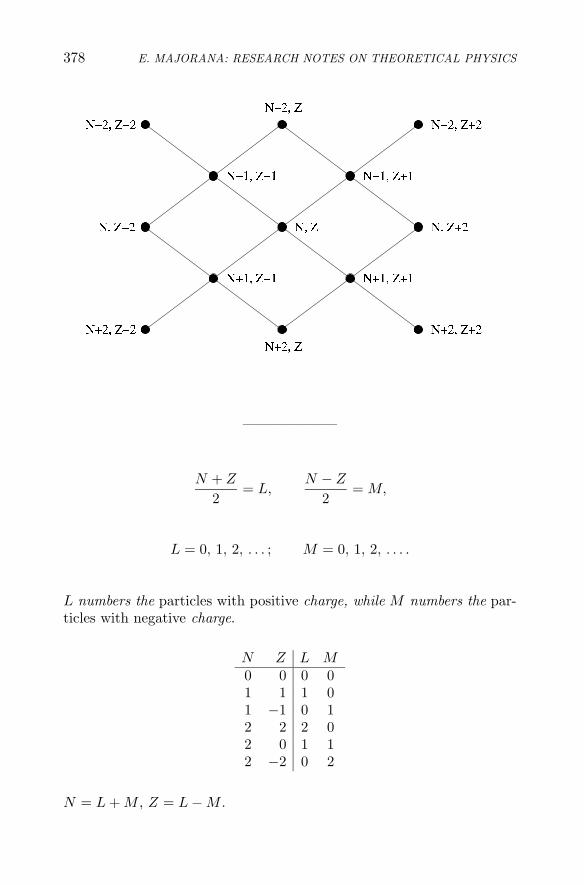
378 E. MAJORANA: RESEARCH NOTES ON THEORETICAL PHYSICS

——————–

N + Z

2= L,

N − Z

2= M,

L = 0, 1, 2, . . . ; M = 0, 1, 2, . . . .

L numbers the particles with positive charge, while M numbers the par-ticles with negative charge.

N Z L M0 0 0 01 1 1 01 −1 0 12 2 2 02 0 1 12 −2 0 2

N = L + M , Z = L − M .

NUCLEAR PHYSICS 379

N Z N + 1 Z + 1

L M L + 1 M

N Z N + 1 Z − 1

L M L M + 1

N Z N − 1 Z + 1

L M L M − 1

N Z N − 1 Z − 1

L M L − 1 M

P0(L,M ;L′,M ′) =√

L + 12

δL+1,L′ δMM ′ +√

L

2δL−1,L′ δMM ′

+√

M + 12

δLL′ δM+1,M ′ +√

M

2δLL′ δM−1,M ′ .

√2 P0 = PL

0 + PM0 = PL + PM ,√

2 Q0 = QL0 + QM

0 = QL + QM ,√2 P1 = QL

0 − QM0 = QL − QM ,√

2 Q1 = −PL0 + PM

0 = −PL + PM .

PL0√2

=

∣∣∣∣∣∣∣∣∣∣∣∣∣∣∣∣∣∣∣∣∣∣∣∣

012

0 0 0 . . .

−12

0√

22

0 0 . . .

0√

22

0√

32

0 . . .

0 0√

32

0 1 . . .

. . . . . . . . . . . . . . . . . .

∣∣∣∣∣∣∣∣∣∣∣∣∣∣∣∣∣∣∣∣∣∣∣∣

,

380 E. MAJORANA: RESEARCH NOTES ON THEORETICAL PHYSICS

QL0√2

=

∣∣∣∣∣∣∣∣∣∣∣∣∣∣∣∣∣∣∣∣∣∣∣∣

0i

20 0 0 . . .

− i

20 i

√2

20 0 . . .

0 −i

√2

20 i

√3

20 . . .

0 0 −i

√3

20 i . . .

. . . . . . . . . . . . . . . . . .

∣∣∣∣∣∣∣∣∣∣∣∣∣∣∣∣∣∣∣∣∣∣∣∣

.

[26]

PL0 QL

0 − QL0 PL

0 = −i.

√2 PL = P0 − Q1,√2 QL = Q0 + P1,√2 PM = P0 + Q1,√2 QM = Q0 − P1.

For h = 2π, ν = 1/2π:

W

hν=

12P 2

L +12Q2

L +12P 2

M +12Q2

M ,

N = L + M =12P 2

L +12Q2

L − 12

+12P 2

M +12Q2

M − 12,

L =12P 2

L +12Q2

L − 12, M =

12P 2

M +12Q2

M − 12,

Z = L − M = Q0P1 − Q1P0 =12P 2

L +12Q2

L − 12P 2

M − 12Q2

M .

——————–

26@ Notice that, by using the matrices given above, the following relation is not actuallysatisfied.

NUCLEAR PHYSICS 381

ψP =14{ψLPL + ψMPM + ψLPM + ψMPL

− PLψL − PMψM + PLψM + PMψL

+ i(ψ2

L + P 2L − ψ2

M − P 2M

−ψLψM + ψMψL + PLPM − PMPL)} .

——————–

Versuchsweise: 27

PM = ψM = 0

(mc2 = 1, h = 2π).

[ψ, P ] =12, [ψ, ψ] = −i, [P, P ] =

i

4.

We have, thus, the classical theory! 28

ψψ =ψ2

L + P 2L

2,

PP =ψ2

L + P 2L

8=

14ψψ,

ψP =i

4(ψ2

L + P 2L).

27@ This German word means “tentatively”, and refers to the successive assumptions. Note,however, that in the original paper the cited word is written as “versucherweiser”.28@ That is, a theory with only positively charged particle, without antiparticles.

PART IV

8

CLASSICAL PHYSICS

8.1. SURFACE WAVES IN A LIQUID

The author studied the propagation of surface waves in liquids under theaction of the gravitational potential U and the liquid pressure P . Someparticular cases were considered in detail.

μα = μF − ∇ p.

F = ∇ U :

α = ∇ U − 1μ

∇ p.

μ = μ(p);

P

∫dp

μ, ∇ P =

1μ

∇ p.

α = ∇ (U − P ).

v = ∇ ϕ,

α = ∇ ∂ϕ

∂t+ vx∇ ∂ϕ

∂x+ vy ∇ ∂ϕ

∂y+ vz ∇ ∂y

∂r

= ∇ ∂ϕ

∂t+

12

∇ V 2.

∇ ∂ϕ

∂t+ ∇ 1

2V 2 − ∇U + ∇ P = 0,

∂ϕ

∂t+

12V 2 − U + P = 0.

For a liquid:

385

386 E. MAJORANA: RESEARCH NOTES ON THEORETICAL PHYSICS

U = g z, P =p

μ.

∂ϕ

∂t+

12V 2 − g z +

p

μ= 0,

∇2 ϕ = 0.

ϕ = Aeωi(t−x/v)ekiz.

∇2 ϕ = −ϕ

(ω2

v2+ k2

).

Since ∇2 ϕ = 0, we have:

k = ±ω

vi,

ϕ = eωi(t−x/v)(Aeωzv + Be−ωzv

).

For small amplitudes:

∂ϕ

∂t− g z +

p

μ= 0.

For z = 0,dp

dt= 0:

∂2ϕ

∂t2− g

∂ϕ

∂z= 0.

For z = �:

∂ϕ

∂z= 0.

−ω2eωi(t−x/v)(A + B) = gω

v(A − B)eωi(t−x/v),

g

v(A − B) = −ω(A + B).

Aeω�/v − Be−ω�/v = 0,

B = Ae2ω�v.

CLASSICAL PHYSICS 387

B + A

B − A=

g

ωv.

g

ωv=

eω�v + e−ω�v

eω�v − e−ω�v.

λ = v/ ω

2π=

2πv

ω,

v

ω=

λ

2π,

v = ωλ

2π, ω = v

2π

λ.

λ

2π

g

v2=

e2π�/λ + e−2π�/λ

e2π�/λ − e−2π�/λ,

2π

λ

v2

g=

e2π�/λ − e−2π�/λ

e2π�/λ + e−2π�/λ= tanh

2π�

λ,

v2 = gλ

2πtanh

2π�

λ, v =

√

gλ

2πtanh

2π�

λ.

For � � λ

2π:

v =√

g �.

For � � λ

2π:

v =

√

gλ

2π.

8.2. THOMSON’S METHOD FOR THEDETERMINATION OF e/m

The equations of motion for the electron moving in the Thomson appa-ratus, aimed at the determination of the charge to mass ratio, e/m, arestudied by the author in these pages.

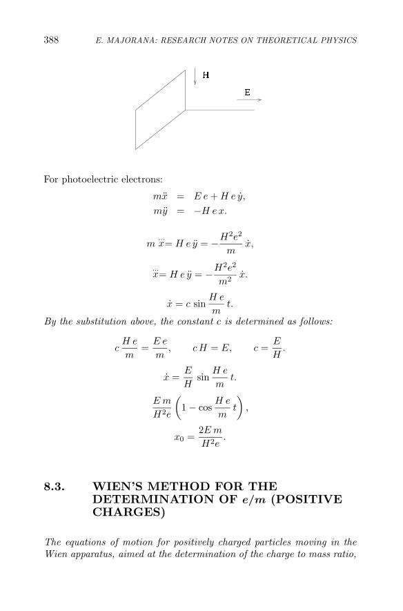
388 E. MAJORANA: RESEARCH NOTES ON THEORETICAL PHYSICS

For photoelectric electrons:

mx = E e + H e y,

my = −H ex.

m...x= H e y = −H2e2

mx,

...x= H e y = −H2e2

m2x.

x = c sinH e

mt.

By the substitution above, the constant c is determined as follows:

cH e

m=

E e

m, cH = E, c =

E

H.

x =E

Hsin

H e

mt.

E m

H2e

(1 − cos

H e

mt

),

x0 =2E m

H2e.

8.3. WIEN’S METHOD FOR THEDETERMINATION OF e/m (POSITIVECHARGES)

The equations of motion for positively charged particles moving in theWien apparatus, aimed at the determination of the charge to mass ratio,

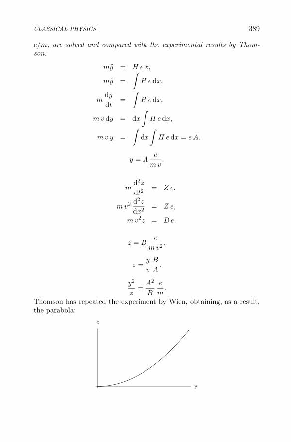
CLASSICAL PHYSICS 389

e/m, are solved and compared with the experimental results by Thom-son.

my = H ex,

my =∫

H edx,

mdy

dt=

∫H edx,

mv dy = dx

∫H edx,

mv y =∫

dx

∫H edx = eA.

y = Ae

mv.

md2z

dt2= Z e,

mv2 d2z

dx2= Z e,

mv2z = B e.

z = Be

mv2.

z =y

v

B

A.

y2

z=

A2

B

e

m.

Thomson has repeated the experiment by Wien, obtaining, as a result,the parabola:

y

Z

390 E. MAJORANA: RESEARCH NOTES ON THEORETICAL PHYSICS

mv2max = 2V e,

zmin =B

2V.

8.4. DETERMINATION OF THE ELECTRONCHARGE

In the following, the author studied several electrical effects in gases,with particular reference to the Townsend effect, that is, the increaseof the photoelectric saturation current from an electrode as a functionof the distance d between plane parallel electrodes for high values of theelectric field (whose strength was denoted with X). The quantity n givesthe number of electric charges (electrons) per unit volume, while theTownsend coefficient α is the number of new ion pairs produced per cen-timeter of path in the gas by electron impacts. The gas is at the pressurep and temperature T , while D is a diffusion coefficient.This study was aimed to obtain determinations of the electron charge e(with different experimental methods).

8.4.1 Townsend Effect

8.4.1.1 Ion recombination.dn

dt=

dm

dt= q − α m n. (1)

CLASSICAL PHYSICS 391

n = m:dn

dt= q − αn2. (2)

q − αn2 = 0; n0 =√

q

α. (3)

dn

q − αn2= dt,

dn

2√

q

(1

√q + n

√α

+1

√q − n

√α

)= dt,

12√

qαlog

√q + n

√α

√q − n

√α

= t,

√q + n

√α

√q − n

√α

= e2t√

qα =e2t

√qα

1,

n

√α

q=

e2t√

qα − 1e2t

√qα + 1

,

n =√

q

α

e2t√

qα − 1e2t

√qα + 1

,

n = n0e√

4αqt − 1e√

4αqt + 1.

n = n0e2n0αt − 1e2n0αt + 1

(4)

(formula applying to a source active for a time t).

——————–

dn

dt= −αn2,

dn

n2= −α dt,

1n0

− 1n

= −αt,

1n

=1n0

+ αt,

n =1

1n0

+ αt=

n0

1 + n0αt(5)

392 E. MAJORANA: RESEARCH NOTES ON THEORETICAL PHYSICS

(formula applying to a source extinguished at time t).

——————–

For the determination of α we can use the following setup, where iA, iBare the saturation currents measured by setting alternately the electrical

tension in A and B, respectively, with iB =12

iA.

V = σv, T = d/v.nB =

nA

1 + nAαT,

and since nB =12

nA,nAαT = 1.

iA = nAV e, iAαT = V e.

α =V e

iAT.

For air we have α = 1.65 · 10−6 = 3480e (Townsend).

8.4.1.2 Ion diffusion.dn

dt= q − αn2 + D∇2 n.

dn

dt= q − αn2 + D

d2n

dx2.

Fordn

dt= 0 and neglecting α,

Dd2n

dx2− q = 0,

d2n

dx2= − q

D,

n =q

2D

(�2 − x2

).

CLASSICAL PHYSICS 393

∫n dx =

q�3

D− 1

3q�3

D=

23

q

D�3.

Q =23

q

D�3e.

Q = 2q � t,13

�2

De = t.

D coefficients (Townsend)+ ions - ions

dry air 0.028 0.043wet air 0.032 0.026dry CO2 0.023 0.026dry H2 0.123 0.190

8.4.1.3 Velocity in the electric field.

N1 = Ddn

dx, N1 = V n.

V n = Ddn

dx, V = D

1n

dn

dx, V = D

1p

dp

dx,

V =D

pn e X.

p = n kT,n

p=

1kT

=N

π,

[1]

V = DN

πeX =

D

kTeX,

The relation utilized by Townsend relation is for X = 1:

V = DN

πe =

D

kTe.

8.4.1.4 Charge of an ion.

n = DN

πe,

N e =πn

D,

1N is the total number of charged particles, while π is the atmospheric pressure (see below).

394 E. MAJORANA: RESEARCH NOTES ON THEORETICAL PHYSICS

where π is the atmospheric pressure. Townsend has found:

Ne′ =96540 · 3 109

22400= 1.3 · 1010,

e

e′= 1.04.

8.4.2 Method of the Electrolysis (Townsend)The oxygen and hydrogen which are formed at the electrode are stronglyelectrified, positively or negatively depending on the kind of electrolysis.From the Stokes law:

v = k a2.

n = q

/43πa3 .

e =Q

n,

where q is evaluated thermodynamically.

8.4.3 Zaliny’s Method For The Ratio Of TheMobility Coefficients

V − k u = 0,

V − k1 v = 0,

u

v=

k1

k=

11.24

.

CLASSICAL PHYSICS 395

Mobility coefficients+ ions - ions ratio T (oC)

dry air 1.36 1.87 1.375 13.5wet air 1.37 1.51 1.10 14dry CO2 0.76 0.81 1.07 17.5wet CO2 0.81 0.75 0.915 17dry H2 6.70 7.95 1.19 20wet H2 5.30 5.60 1.05 20

−y =1y

K

log b/au.

12

b2 − 12

y2 =K

log b/au t =

K

log b/au

x

V.

V(b2 − a2

)=

2K

log b/au x.

Q = π(b2 − a2

)V, Q =

2Kπ

log b/au x.

u =Q log b/a

2πKx.

8.4.4 Thomson’s Method

396 E. MAJORANA: RESEARCH NOTES ON THEORETICAL PHYSICS

8.4.5 Wilson’s MethodIt is as the Thomson’s method, with the addition of an electric field tothe gravity. The charge e is obtained from the ratio between the fallvelocities with and without the field:

v1

v=

43πρ g a3 + Xe

43πρ g a3

.

By determining a from the Stokes formula (see below), we van obtainthe value of e.

8.4.6 Millikan’s Method

The Stokes law:

v =29

ga2

μ(σ − ρ)

has been corrected by Cunningham for droplets with small radius:

v =29

ga2

μ(σ − ρ)

(1 + A

�

a

),

where A is a numerical constant and � is the mean free path. By settingB = A� we have:

v =29

ga2

μ(σ − ρ)

(1 +

B

a

).

CLASSICAL PHYSICS 397

8.5. ELECTROMAGNETIC ANDELECTROSTATIC MASS OF THEELECTRON

The expressions for the electromagnetic and the electrostatic mass ofthe electron are derived, by evaluating the magnetic energy W and theanalogous electrostatic energy W/c2.

H =e u sin θ

r2,

H2 =e2 u2 sin2 θ

r4,

H2

8π=

e2 u2 sin2 θ

8πr4.

4πr2 H2

8πdr =

e2u2

3r2dr.

∫ ∞

a

dr

r2=

1a.

W =e2u2

3a=

12

mu2.

m =23

e2

a(electromagnetic),

m =23

e2

a c2(electrostatic).

8.6. THERMIONIC EFFECT

In the following the author studied electron emission induced by therm-ionic effect, obtaining the Richardson formula for the electron current.Moreover, he subsequently considered also the Langmuir effect (for lowvoltage) induced by the cloud of (slowly moving) electrons (space charge)around the cathode, which limits the electron emission from the cathode.

398 E. MAJORANA: RESEARCH NOTES ON THEORETICAL PHYSICS

Let V e be the extraction work; in order that an electron comes out ofthe metal, the following relation must hold:

V e ≤ 12

mu2.

The Maxwell distribution gives:

dn = C e−m u2/kT du,

dn = n

√hm

πe−h m u2

du,

h = 1/2kT .

V e =12

mu20, u0 =

√2 V e

m.

The number of electrons emitted is then given by:

∫ ∞√

2V e/m2 dn = 2n

√hm

π

∫ ∞√

2V e/me−h m u2

du

= n

√hm

π

1hm

√2 V E/m

e−b/T

= n

√1

2 V e hπe−b/T

= n

√kT

π V ee−b/T .

From this, the Richardson formula for the electron current i follows(Richardson effect):

i = aT 1/2 e−b/T .

Instead, with the photoelectric theory, it has been found that:

i = aT 2 e−b/T .

Electron emission starts around 1000oC; for several elements (sodium)it starts around 200oC. If T is small, the value for the saturation currentis reached very quickly.

——————–

CLASSICAL PHYSICS 399

V e =12

mu2.

V = u/300:

u

300e =

12

mu2,

u =√

u

√2e

300m.

e = 4.77 · 10−10, m = 0.9 · 10−27,

2e

300m= 5.53 · 1015,

u =√

u · 594 km/s.

8.6.1 Langmuir Experiment on the Effect of theElectron Cloud

At low values of the potential, the electron current does not change withvarying T .

d2V

dx2= −4πρ.

i = ρ v = const.

v = k√

V , −4πρ =c√V

.

d2V

dx2=

c√V

,

d2V

dx2=

ddx

dV

dx;

ddV

dx=

c√V

dx,

dV

dxd

dV

dx=

c√V

.

(dV

dx

)2

= c√

V + const.

400 E. MAJORANA: RESEARCH NOTES ON THEORETICAL PHYSICS

V (0) = 0, V (�) = V1.

v = v0

√V , ρ =

i

v0

√V

.

[2]

i = kV 3/2

x2.

——————–

Effects that are an obstacle to the reaching of the value of the saturationcurrent are the following.1) the cloud of slowly moving electrons around the cathode (Langmuireffect):

imax = k V 3/2;

2) the magnetic field produced by the filament (a voltage of the order of1 volt is required):

m x = E e − H z,

m z = H x,

E =A

x, H =

B

x,

m x =A

xe − B

xz, mx x = A e − B z,

m z =B

xx;

3) a non-vanishing gradient of the voltage along the filament (of theorder of 1 volt/cm).

2@ It is not clear how the author solved the differential equation for V , thus obtaining theexpression for ρ and, finally, the following expression for the current i. Nevertheless, theexpression for i is correct, choosing in a given way the integration constant in the differentialequation above.

CLASSICAL PHYSICS 401

If the effects 1), 2) and 3) are removed in some way, the saturation ofthe current is reached at a very lower voltage. This has been verifiedexperimentally by Schottky.3 The effect 3) is removed by switching offthe voltage and measuring i at the same time instant.

3In the original manuscript, the author writes this name (between brackets) as “Sciochi”.

9

MATHEMATICAL PHYSICS

In the following six Sections, the author studied a number of topics deal-ing with tensor calculus, following closely the text T. Levi-Civita, Lezionidi calcolo differenziale assoluto (Stock, Rome, 1925), which was presentin the Majorana personal library. For the notations used and furthercomments on the topics treated, we refer the reader to this book (wedenote it as Levi-Civita I) or to its English translation (denoted as Levi-Civita E) in T. Levi-Civita, The Absolute Differential Calculus – Calcu-lus of Tensors (Blackie & Son, London, 1926). Some explicit referencesto chapters (III and IV) or pages (pp. 48, 60, 123, 137, 140, 141, 143,160, 173, 174, 178, 197 of Levi-Civita I or pp. 36, 47, 107, 119, 121,123, 131, 140, 152, 153, 156, 172 of Levi-Civita E) of this book are re-ported throughout the manuscript. A few results, on the contrary, do notappear in the mentioned book; they were obtained by Majorana, or hesimply reported what was expounded in the university course taught byLevi-Civita at the University of Rome and followed by Majorana himself.

9.1. LINEAR PARTIAL DIFFERENTIALEQUATIONS. COMPLETE SYSTEMS

X1, . . . , Xn:

∑Xidxi = 0.

y(x1, . . . , xn) = C,

dy =∑ ∂y

∂xidxi.

∂y

∂xi= pXi, p = p(x1 . . . xn).

403

404 E. MAJORANA: RESEARCH NOTES ON THEORETICAL PHYSICS

dy =∑

pXidxi =∑

Aidxi.

∂Ai

∂xj− ∂Aj

∂xi= 0.

p

(∂Xi

∂xj− ∂Xj

∂xi

)+ Xi

∂p

∂xj− Xj

∂p

∂xi= 0,

p

(∂Xj

∂xk− ∂Xk

∂xj

)+ Xj

∂p

∂xk− Xk

∂p

∂xj= 0,

p

(∂Xk

∂xi− ∂Xi

∂xk

)+ Xk

∂p

∂xi− Xi

∂p

∂xk= 0;

Xk

(∂Xi

∂xj− ∂Xj

∂xk

)+ Xi

(∂Xj

∂xk− ∂Xk

∂xj

)+ Xj

(∂Xk

∂xi− ∂Xi

∂xk

)= 0.

9.1.1 Linear Operators

Auv = vAu + uAv = (−Au)v + uAv.

A =N∑

r=1

ar∂

∂xr, B =

N∑

r=1

br∂

∂xr.

AB =N∑

r,s=1

ar∂

∂xr

(bs

∂

∂xs

)

=N∑

r,s=1

arbs∂2

∂xr∂xs+

N∑

r,s=1

ar∂bs

∂xr

∂

∂xs,

BA =N∑

r,s=1

arbs∂2

∂xr∂xs+

N∑

r,s=1

br∂as

∂xr

∂

∂xs,

AB − BA = (A,B) =N∑

r,s=1

(ar

∂bs

∂xr− br

∂as

∂xr

)∂

∂xs.

MATHEMATICAL PHYSICS 405

AB =∑

rs

arbs∂2

∂xr∂xs+∑

s

(Abs)∂

∂xs,

BA =∑

rs

arbs∂2

∂xr∂xs+∑

s

(Bas)∂

∂xs,

AB − BA = (A,B) =N∑

s=1

(Abs − Bas)∂

∂xs.

——————–

A1, . . . , An:

B =n∑

1

λiAi, C =n∑

1

μiAi.

BC =n∑

i,k=1

λiAiμkAk =∑

i,k

λiμkAiAk +∑

i,k

λi(Aiμk)Ak,

CB =∑

i,k

λiμkAkAi −∑

i,k

μi(Aiλk)Ak,

(B.C) = BC − CB

=∑

i,k

λiμk(Ai, Ak) +∑

k

[∑

i

(λiAiμk − μiAiλk)

]

Ak.

9.1.2 Integrals Of An Ordinary DifferentialSystem And The Partial DifferentialEquation Which Determines Them

x1, . . . , xn:

dxi

dt= Xi(x|t). (1)

f(x|t) = constant:

∂f

∂t+∑ ∂f

∂xi

dxi

dt= 0,

∂f

∂t+∑ ∂f

∂xiXi = 0.

406 E. MAJORANA: RESEARCH NOTES ON THEORETICAL PHYSICS

A =∂

∂t+∑

Xi∂

∂xi,

Af = 0.

f(x|t) constant for any value of of 1 implies Af = 0.Conversely, Af = 0 implies f(x|t) constant for any value of of 1.

9.1.3 Integrals Of A Total Differential SystemAnd The Associated System Of PartialDifferential Equation That DeterminesThem

duα =n∑

1

Xαidxi, α = 1, . . . , m.

f(x|u) = constant:

df =∑ ∂f

∂xidxi +

∑ ∂f

∂uαduα

=n∑

i=1

(∂f

∂xi+

m∑

α=1

∂f

∂uαXαi

)

dxi.

∂f

∂xi+

m∑

α=1

∂f

∂uαXαi = 0 (i = 1, 2, . . . , n).

Ωi =m∑

α=1

Xαi∂

∂uα.

Bi =∂

∂xi+ Ωi, (i = 1, 2, . . . , n).

Bif = 0, (i = 1, 2, . . . n).

——————–

Complete systems:

Akf = 0,

MATHEMATICAL PHYSICS 407

Ak =N∑

1

akν∂

∂xν(k = 1, 2, . . . , n);

(Ai, Ak) =n∑

1

piklAl, pikl = −pkil.

Jacobian systems:(Ai, Ak) = 0.

Reduction of a complete system to a Jacobian one:

Bif =n∑

k=1

cikAkf, ‖cik‖ �= 0.

N − n = m; xn+1 = u1, xn+2 = u2, . . . xN = um:

Akf =N∑

1

aki∂f

∂xi=

m∑

1

aki∂f

∂xi+ Ukf = 0,

Uk =m∑

r=1

ak,n+r∂

∂ur.

n∑

i=1

aki∂f

∂xi+ Ukf = 0, k = 1, 2, . . . , n, ‖aki‖ �= 0;

n∑

i=1

aki∂f

∂xi= −Ukf.

n∑

i=1

αkraki∂f

∂xi= −αkrUkf,

where αri =Ari

Ais the reciprocal element of ari:∑

i

αriaki = δik,∑

i

αkiakr = δir.

n∑

i=1

n∑

r=1

αkraki∂f

∂xi=

n∑

i=1

δir∂f

∂xi

=∂f

∂xr= −

n∑

r=1

αkrUkf,

408 E. MAJORANA: RESEARCH NOTES ON THEORETICAL PHYSICS

that is a Jacobian system.Conversely, let us start from a Jacobian system:

∂f

∂xi+ Ωif = 0, i = 1, 2, . . . n,

where Ωi are linear operators depending only on u1, . . . , um,

Ωi =m∑

α=1

Xiα∂

∂uα.

By setting:

Bi =∂

∂xi+ Ωi,

we have:

Bif = 0, i = 1, 2, . . . , n,

Bi =∑

i

αkiAk.

The Poisson brackets of the B operators are linear combinations of thePoisson brackets of the A operators and of the A themselves, and sincethe A operators define a complete system and, in turn, are combinationsof the B operators, we have:

(Bi, Bk) =∑

i

qik�B�.

Bi =∂

∂xi+ Ωi, Bk =

∂

∂xk+ Ωk.

BiBk =∂2

∂xi∂xk+ Ωi

∂

∂xk+

∂

∂xiΩk + ΩiΩk,

BkBi =∂2

∂xi∂xk+ Ωk

∂

∂xi+

∂

∂xkΩi + ΩkΩi,

(Bi, Bk) =(

Ωi∂

∂xk− ∂

∂xkΩi

)+(

∂

∂xiΩk − Ωk

∂

∂xi

)+ ΩiΩk − ΩkΩi

= Ωik = 0.

MATHEMATICAL PHYSICS 409

9.2. ALGEBRAIC FOUNDATIONS OF THETENSOR CALCULUS

9.2.1 Covariant And Contravariant Vectors

S : x −→ x,

S−1∗ : u −→ u′.

Covariant:

u′i = uk

∂xk

∂x′i

, u′′i u

′k

∂x′k

∂x′′i

= ur∂xr

∂x′k

∂x′k

∂x′′i

= ur∂xr

∂x′′i

= uk∂xk

∂x′′i

.

Contravariant:

u′i = uk ∂x′i

∂xk, u′′iu′k ∂x′′i

∂x′k = ur∂x′′k

∂xr

∂x′′i

∂x′k = ur ∂x′′i

∂xr= uk ∂x′′i

∂xk.

9.3. GEOMETRICAL INTRODUCTION TOTHE THEORY OF DIFFERENTIALQUADRATIC FORMS I

9.3.1 The Symbolic Equation Of Parallelism

dR · δP = 0

(δP taken on the surface);

3∑

ν=1

dYν δyν = 0

(δyν being the most general ones).

9.3.2 Intrinsic Equations Of ParallelismDeduction of the intrinsic equations:

δyν =2∑

k=1

∂yν

∂xk∂xk,

Yν =2∑

i=1

∂yν

∂xiRi

410 E. MAJORANA: RESEARCH NOTES ON THEORETICAL PHYSICS

(Ri = Rλi; R is the length of the vector; λi = dxi/ds),

R2 =∑

aikRiRk.

2∑

ν=1

dyν δyν =3∑

ν=1

2∑

i=1

d(

∂yν

∂xiRi

) 2∑

k=1

∂yν

∂xνδxk

=∑

k

τkδrk = 0,

τk =3∑

ν=1

2∑

i=1

∂yν

∂xkd(

∂yν

∂xiRi

).

τk = 0.

τk =3∑

ν=1

2∑

i=1

∂yν

∂xk

∂yν

∂xidRi +

3∑

ν=1

2∑

i=1

2∑

j=1

Ri ∂yν

∂xk

∂2yν

∂xi∂xjdxj

=2∑

i=1

aikdRi +2∑

i,j=1

Ridxj

3∑

ν=1

∂yν

∂xk

∂2yν

∂xi∂xj

=2∑

i=1

aikdRi +2∑

i,j=1

Ridxj

⎡

⎣i j

k

⎤

⎦ .

3∑

ν=1

∂yν

∂xk

∂2yν

∂xi∂xj=∑

ν

∂

∂xj

∂yν

∂xk

∂yν

∂xi−∑

ν

∂yν

∂xi

∂2yν

∂xk∂xj.

⎡

⎣i j

k

⎤

⎦ =∂

∂xjaik −

⎡

⎣k j

i

⎤

⎦ ,

⎡

⎣i j

k

⎤

⎦+

⎡

⎣j k

i

⎤

⎦ =∂

∂xjaik,

⎡

⎣j k

i

⎤

⎦+

⎡

⎣k i

j

⎤

⎦ =∂

∂xkaji,

⎡

⎣k i

j

⎤

⎦+

⎡

⎣i j

k

⎤

⎦ =∂

∂xiakj ,

MATHEMATICAL PHYSICS 411

⎡

⎣i j

k

⎤

⎦ =12

(∂

∂xiaki +

∂

∂xjaki −

∂

∂xkaij

).

dR · δP =∑

τk δxk, τk = 0,

τk =2∑

i=1

aik dRi +2∑

i,j=1

⎡

⎣i j

k

⎤

⎦Ridxj = 0.

τk is a covariant vector; in fact,∑

τkδxk = invariant.

τ � =∑

k

a�kτk,

τ � is a contravariant vector.

τ � = dRi +2∑

i,j=1

⎧⎨

⎩

i j

�

⎫⎬

⎭Ridxj = 0.

dR� = −2∑

i,j=1

⎧⎨

⎩

i j

�

⎫⎬

⎭Ridxj

(which is the equation of the parallelism).

9.3.3 Christoffel’s Symbols

⎡

⎣j �

k

⎤

⎦ =12

(∂

∂xja�k +

∂

∂x�akj −

∂

∂xkaj�

),

⎧⎨

⎩

j �

i

⎫⎬

⎭=∑

k

aik

⎡

⎣j �

k

⎤

⎦ ,

⎡

⎣j �

k

⎤

⎦ =

⎡

⎣� j

k

⎤

⎦ ,

⎧⎨

⎩

j �

i

⎫⎬

⎭=

⎧⎨

⎩

� j

i

⎫⎬

⎭;

∂aik

∂xj=

⎡

⎣j k

i

⎤

⎦+

⎡

⎣j i

k

⎤

⎦ ,

412 E. MAJORANA: RESEARCH NOTES ON THEORETICAL PHYSICS

⎡

⎣j �

k

⎤

⎦ =∑

aik

⎧⎨

⎩

j �

i

⎫⎬

⎭.

——————–

a =

∣∣∣∣∣∣

a11 . . . a1n

. . .an1 . . . ann

∣∣∣∣∣∣.

∂a

∂xi=∑

r,s

∂ars

∂xi

ars

a,

∂ log a

∂xi=∑

r,s

ars ∂ars

∂xi=∑

r,s

ars

⎛

⎝

⎡

⎣i r

s

⎤

⎦+

⎡

⎣i s

r

⎤

⎦

⎞

⎠

=∑

r

⎧⎨

⎩

i r

r

⎫⎬

⎭+∑

s

⎧⎨

⎩

i s

s

⎫⎬

⎭= 2∑

r

⎧⎨

⎩

i r

r

⎫⎬

⎭,

∂ log√

a

∂xi=∑

r

⎧⎨

⎩

i r

r

⎫⎬

⎭.

9.3.4 Equations Of Parallelism In Terms OfCovariant Components

dR� = −∑

ij

⎧⎨

⎩

i j

�

⎫⎬

⎭Ridxj (contravariant components),

Rs =∑

as�R�,

dRs =∑

�

as� dRl +∑

�

R� das�,

das� =∑

t

∂asl

∂xtdxt =

∑

t

⎛

⎝

⎡

⎣t s

�

⎤

⎦+

⎡

⎣t �

s

⎤

⎦

⎞

⎠Rldxt,

MATHEMATICAL PHYSICS 413

dRs =∑

�

as� dR� +∑

�,t

R�

⎛

⎝

⎡

⎣t s

�

⎤

⎦+

⎡

⎣t �

s

⎤

⎦

⎞

⎠dxt

= −∑

i,j

⎡

⎣i j

s

⎤

⎦Ridxj +∑

�,t

R�

⎛

⎝

⎡

⎣t s

�

⎤

⎦+

⎡

⎣t �

s

⎤

⎦

⎞

⎠dxt

=∑

�,t

R�

⎡

⎣t s

�

⎤

⎦ dxt.

⎡

⎣t s

�

⎤

⎦ =∑

r

a�r

⎧⎨

⎩

t s

r

⎫⎬

⎭,

dRs =∑

�,t,r

a�rR�dxt

⎧⎨

⎩

t s

r

⎫⎬

⎭=∑

t,r

Rrdxt

⎧⎨

⎩

t s

r

⎫⎬

⎭.

Equations of the parallelism

contravariant components : dRi = −∑

�,k

⎧⎨

⎩

� k

i

⎫⎬

⎭R�dxk

covariant components : dRi =∑

�,k

⎧⎨

⎩

i k

�

⎫⎬

⎭R� dxk

9.3.5 Some Analytical Verifications

xi = xi(s), i = 1, 2,

Ri = −2∑

ell=1

⎧⎨

⎩

� k

i

⎫⎬

⎭R�xk

V i = −∑

�,k

⎧⎨

⎩

� k

i

⎫⎬

⎭V �xk;

414 E. MAJORANA: RESEARCH NOTES ON THEORETICAL PHYSICS

∑

i

RiVi = −∑

i,�,k

⎧⎨

⎩

� k

i

⎫⎬

⎭R�Vixk;

Ri =∑

�,k

⎧⎨

⎩

i k

�

⎫⎬

⎭R�xk,

V i =∑

�,k

⎧⎨

⎩

i k

�

⎫⎬

⎭V�xk;

∑RiVi = −

∑

i,�,k

⎧⎨

⎩

� k

i

⎫⎬

⎭R�V�xk,

∑

i

RiV i =∑

i,�,k

⎧⎨

⎩

i k

�

⎫⎬

⎭RiV�xk =

∑

i,�,k

⎧⎨

⎩

� k

i

⎫⎬

⎭R�Vixk,

dds

(R · V ) =dds

∑

i

RiVi =∑

i

RiVi +∑

i

RiVi = 0.

9.3.6 Permutability

dδxi = −∑

k,�

⎧⎨

⎩

k �

i

⎫⎬

⎭δxk dx�, δxi = −

∑

k,�

⎧⎨

⎩

k �

i

⎫⎬

⎭dxk δx�,

dδxi = δdxi.

xi + dxi + δxi + dδxi = xi + δxi + dxi + δdxi.

9.3.7 Line Elements

ds2 =n∑

i,k=1

aikdxidxk.

λi =dxi

ds, λi =

n∑

k=1

aikλk, λi =

∑aikλk,

MATHEMATICAL PHYSICS 415

n∑

i,k=1

aikλiλk =

n∑

i=1

λiλi =n∑

i,k=1

aikλiλk = 1,

Ri = Rλi, Ri = Rλi,

R2 =n∑

i,k=1

aikRiRk =

n∑

i=1

RiRi =n∑

i,k=1

aikRiRk.

cos θ =n∑

i,k=1

aikλiμk =

n∑

i=1

λiμi =n∑

k=1

λkμk =n∑

i,k=1

aikλiμk,

R · V =n∑

i=1

RiVi.

9.3.8 Euclidean Manifolds. Any Vn Can AlwaysBe Considered As Immersed In AEuclidean Space

Wp (immersed in Vn):

xi = fi(ui, . . . , up) (i = 1, 2, . . . , n; p < n).

ds2 =n∑

i,k=1

aikdxidxk =n∑

i,k=1

p∑

r,s=1

aik∂xi

∂ur

∂xk

∂usdurdus

=p∑

r,s=1

brsdurdus,

brs =n∑

i,k=1

aik∂xi

∂ur

∂xk

∂us.

——————–

An arbitrary Vn can always be considered as immersed in a Euclideanspace.Vn immersed in SN , N > n.

416 E. MAJORANA: RESEARCH NOTES ON THEORETICAL PHYSICS

y1(x), y2(x), . . . , yN (x).

n∑

i,k=1

aikdxidxk =N∑

ν=1

dy2ν ,

dyν =n∑

i=1

∂yν

∂xidxi =

n∑

k=1

∂yν

∂xkdxk,

dy2ν =

n∑

i,k=1

∂yν

∂xi

dyν

dxkdxidxk.

n∑

i,k=1

aikdxidxk =N∑

ν=1

n∑

i,k=1

dyν

∂xi

∂yν

∂xkdxidxk,

aik =N∑

ν=1

∂yν

∂xi

∂yν

∂xk(i, k = 1, 2, . . . , n).

If N =n(n + 1)

2, the problem has a solution.

n N = n(n + 1)/21 12 33 64 10

C = min(N − n),

min N ≤ n(n + 1)2

,

C ≤ n(n + 1)2

− n =n(n − 1)

2.

n max (Nmin) Cmax

n(n + 1)/2 n(n − 1)/21 1 02 3 13 6 34 10 6

9.3.9 Angular Metric

R2 =∑

aikRiRk, V 2 =

∑aikV

iV k,

MATHEMATICAL PHYSICS 417

|R + V |2 =∑

aik(Ri + V i)(Rk + V k) = R2 + V 2 + 2∑

aikRiV k,

R · V =∑

i,k

aikRiV k =

∑

i

RiVi =∑

i

RiVi =∑

ik

aikRiVk.

For a definite form a, and taking xi and yi not proportional, it follows:∣∣∣∑

aikxiyk

∣∣∣2

<∑

aikxixk ·∑

aikyiyk.

zi = λxi + μyi.

∑aikzizk > 0,

λ2∑

aikxixk + 2λμ∑

aikxiyk + μ2∑

aikyiyk > 0,

(∑aikxiyk

)2<∑

aikxixk ·∑

aikyiyk.

cos θ =n∑

i,k=1

aikλiμk =

n∑

i=1

λiμi =n∑

i=1

λiμi =

n∑

i,k=1

aikλiμk,

R · V =∑

aikRiV k =

∑RiVi =

∑RiV

i =∑

aikRiVk.

9.3.10 Coordinate LinesFor the coordinate line i (aj = constant for j �= i), the parameters λi

are:

λj =dxj

ds=

⎧⎨

⎩

0 (j �= i),

1/√

aii (j = i).

The moments of the normal to the surface xi = constant are:

μj = 0 for j �= i, μi =1√aii

.

The angle between the coordinate lines i and k is given by:

cos θ =∑

arsλrλ′s =

aik√aiiakk

.

418 E. MAJORANA: RESEARCH NOTES ON THEORETICAL PHYSICS

The angle between the hypersurfaces xi = constant and xk = constantis given by:

cos θ =aik

√aiiakk

.

Let si be a unitary vector along the line i (the parameters are then equalto the contravariant components: λj = 0 for j �= i, λi = 1/

√aii).

Let ni be a unitary vector normal to the hypersurface xi = constant (themoments are then equal to the covariant components: μj = 0 for j �= i,μi = 1/

√aii).

R · si =∑

Rj(si)j =Ri√aii

,

R · ni =∑

Rjni,j =Ri

√aii

;

Ri =√

aii R · si, Ri =√

aii R · ni.

9.3.11 Differential Equations Of Geodesicsxi = xi(t):

s =∫ √

aikdxidxk =∫

ds.

I =∫ B

Ads =

∫ B

A

√aikdxidxk,

δI =∫ B

Aδds.

ds2 =∑

aikdxidxk,

ds δds =∑

aikdxidδxk +12

∑δaik · dxidxk,

δaik =∑ δaik

δxjδxj ,

δds =∑

aikxiδdxk +12

∑

i,k,j

δaik

δxjδxj xixkds.

MATHEMATICAL PHYSICS 419

δI =∫ ∑

aikxiδdxk +12

∫ ∑

i,k,j

δaik

δxjδxj xixkds.

∫ ∑aikxidδxk =

∑aikxiδxk

∣∣∣B

A−∫ B

A

∑

i,k

(aikxi + aikxi)δxk.

δI =∫ B

A

∑

k

δxk ·

⎛

⎝12

∑

i,j

∂aij

δxkxixj −

∑

i

aikxi −∑

i

aikxi

⎞

⎠ds.

——————–

aik =∑

j

∂aik

∂xjxj ,

dI =∫ B

A

∑

k

δxk

⎛

⎝12

∑

i,j

∂aij

∂xkxixj −

∑

i,j

∂aik

∂xjxixj −

∑

i

aikxi

⎞

⎠ds.

dI = −∫

pkδxkds, δI +∫ B

Apkδxkds = 0,

pk =∑

i,j

⎡

⎣i j

k

⎤

⎦ xixj +∑

i

aikxi.

∑

i

aikxi +∑

i,j

⎡

⎣i j

k

⎤

⎦ xixj = 0 (k = 1, 2, . . . , n).

pi =∑

k

aikpk,

pk =∑

i,j

⎧⎨

⎩

i j

k

⎫⎬

⎭xixj + xk.

420 E. MAJORANA: RESEARCH NOTES ON THEORETICAL PHYSICS

Equations of the geodesic lines

dI = −∫

AB

∑pkδxkds, pk =

∑

ij

⎡

⎣i j

k

⎤

⎦ xixj +∑

i

aij xi

pi =∑

aikxk, pk =∑

ij

⎧⎨

⎩

i j

k

⎫⎬

⎭xixj + ak

pk = 0, that is:n∑

i,j=1

⎡

⎣i j

k

⎤

⎦ xixj +n∑

i=1

aikxi = 0

(k = 1, 2, . . . , n),

or

pk = 0, that is: xk +n∑

i,j=1

⎧⎨

⎩

i j

k

⎫⎬

⎭xixj = 0

(k = 1, 2, . . . , n).

9.3.12 Application

ds2 = dx21 + r2dx2

2.

a11 = 1, a22 = r2, a12 = 0;

a11 = 1, a22 =1r2

, a12 = 0.

∂a11

∂x1=

∂a11

∂x2= 0,

∂a22

∂x1=2rr′,

∂a22

∂x2=0,

∂a12

∂x1=

∂a12

∂x2= 0.

⎡

⎣1 1

1

⎤

⎦ =12

(∂a11

∂x1+

∂a11

∂x1− ∂a11

∂x1

)= 0,

⎡

⎣1 2

1

⎤

⎦ =12

(∂a11

∂x2+

∂a12

∂x1− ∂a12

∂x1

)= 0,

MATHEMATICAL PHYSICS 421⎡

⎣2 2

1

⎤

⎦ = −rr′,

⎡

⎣1 1

2

⎤

⎦ = 0,

⎡

⎣1 2

2

⎤

⎦ = rr′,

⎡

⎣2 2

2

⎤

⎦ = 0.

⎧⎨

⎩

1 1

1

⎫⎬

⎭= 0,

⎧⎨

⎩

1 2

1

⎫⎬

⎭= 0,

⎧⎨

⎩

2 2

1

⎫⎬

⎭= −rr′,

⎧⎨

⎩

1 1

2

⎫⎬

⎭= 0,

⎧⎨

⎩

1 2

2

⎫⎬

⎭=

r′

r,

⎧⎨

⎩

2 2

2

⎫⎬

⎭= 0.

x1 − rdr

dx1x2

2 = 0, r2x2 + 2rdr

dx1x1x2 = 0,

or

x1 − rdr

dx1x2

2 = 0, x2 +2r

dr

dx1x1x2 = 0.

sin α = rx2, r sin α = r2x2,

dds

(r sin α) = 2rdr

dx1x1x2 + r2x2 = 0,

r2x2 = constant.

⎧⎪⎪⎪⎨

⎪⎪⎪⎩

x1 = rdr

dx1x2

2, x1 = rdr

dx1

c2

r4,

x2 = −2r

dr

dx1xx2, r2x2 = c.

422 E. MAJORANA: RESEARCH NOTES ON THEORETICAL PHYSICS

9.4. GEOMETRICAL INTRODUCTION TOTHE THEORY OF DIFFERENTIALQUADRATIC FORMS II

9.4.1 Geodesic Curvature[1]xi = xi(s); x1, x2, . . . , xn are the coordinates in the space Vn.

dI = −∫

AB

∑

k

pkδxkds

= −∫

AB

∑

k

pkδxkds;

∫ ∑

k

(pkdxk − pkδxk)ds = 0,

∑

k

pkδxk =∑

k

pkδxk.

geodesic curvature

pk =∑

i

akixi +∑

i,j

⎡

⎣i j

k

⎤

⎦ xixj , covariant components;

pk = xi +∑

i,j

⎧⎨

⎩

i j

k

⎫⎬

⎭xixj , contravariant components.

9.4.2 Vector Displacement

s s + ds

parallel displacement xi xi −∑

i,k

⎧⎨

⎩

l k

i

⎫⎬

⎭xlxk ds = ui

line displacement xi xi + xi ds = vi

1@ In the original manuscript, a reference appears (p. 154) of a unspecified text.

MATHEMATICAL PHYSICS 423

vi − ui =

⎡

⎣∑

�,k

⎧⎨

⎩

� k

i

⎫⎬

⎭xlk

⎤

⎦ds = pids.

ui, ui + pids;xi, xi + pids.

∑aikxixk = 1.

∑aik(aik(ai + pids)(xk + pkds)

= 1 + 2∑

i,k

aikxipkds +

∑

i,k

aikpipkds2,

∑aikxip

k =∑

i,k

aikxixk +∑

i,k,�,m

aik

⎧⎨

⎩

� m

k

⎫⎬

⎭xix�xm

=∑

i,k

aikxixk +∑

i,�,m

⎡

⎣� m

i

⎤

⎦ x�xmxi

=12

⎡

⎣∑

i,k

aikdds

(xixk)

+∑

i,k,�

xixk

(∂ai�

∂xk+

∂ak�

∂xi− ∂aik

∂x�

)x�

⎤

⎦

=12

⎡

⎣∑

i,k

aikdds

(xixk)

+∑

i,k

xixk

(−∂aik

∂s+

∂aik

∂s+

∂aik

∂s

)⎤

⎦

=12

dds

∑aikxixk = 0.

——————–∑

i,k

aikpi = ρ2.

424 E. MAJORANA: RESEARCH NOTES ON THEORETICAL PHYSICS

t · t = 1, t · (t + ρds) = 1,

(t + ρ ds)(t + ρds) = 1 + ρ2ds2;

cos(t, t + ρds) =1

1 + (1/2)ρ2ds= 1 − 1

2ds2,

sin(t, t + ρ ds) = ρds.

9.4.3 Autoparallelism Of Geodesics

pk =∑

aikxi +∑

i,j

⎡

⎣i j

k

⎤

⎦ xixj = 0,

pk = xk +∑

i,j

⎧⎨

⎩

i j

k

⎫⎬

⎭xixj = 0.

λi = xi,

dλk = xds = −∑

i,j

⎧⎨

⎩

i j

k

⎫⎬

⎭λidxj (antiparallelism)

9.4.4 Associated Vectors

V k =dRk

ds+∑

i,j

⎧⎨

⎩

i j

k

⎫⎬

⎭Rixj =

τk

ds

τk = 0 : dRk +∑

i,j

⎧⎨

⎩

i j

k

⎫⎬

⎭Ridxj = 0 (parallelism);

for Rk = xk :

V k = pk = xk +∑

i,j

⎧⎨

⎩

i j

k

⎫⎬

⎭xixj (geodesic curvature);

pk = xk +∑

i,j

⎧⎨

⎩

i j

k

⎫⎬

⎭xixj = 0 (equation of the geodesic lines).

MATHEMATICAL PHYSICS 425

9.4.5 Remarks On The Case Of An Indefiniteds2

ds2 =∑

aikdxidxk, ‖aik‖ �= 0.

time directions: ds2 > 0 (∞n−1);space directions: ds2 < 0 (∞n−1);

null interval directions: ds2 = 0 (∞n−1).

9.5. COVARIANT DIFFERENTIATION.INVARIANTS AND DIFFERENTIALPARAMETERS. LOCALLY GEODESICCOORDINATES

9.5.1 Geodesic Coordinates

xi = xi(x1, x2, . . . , xn) (i = 1, 2, . . . , n).

∂aik

∂xj= 0 (i, k, j = 1, 2, . . . , n).

P = P0(x01, x

02, . . . , x

0n) = P 0(x0

1, x02, . . . , x

0n)

aik =∑

r,s

ars∂xr

∂ri

∂xs

∂xk,

∂aik

∂aj=∑

r,s,t

∂ars

∂xt

∂xr

∂xi

∂xs

∂xk

∂xt

∂xj+∑

r,s

ars∂2xr

∂xi∂xj

∂xs

∂xk

+∑

r,s

ars∂xr

∂xi

∂2xs

∂xk∂xj.

∂xi

∂xk= aik, dxi =

∑aikdxk,

dx = Sdx.

x = Ux′, dx = Udx′,

426 E. MAJORANA: RESEARCH NOTES ON THEORETICAL PHYSICS

dx = S Udx.

P P0

xr = xr +12

∑

i,k

qrikxixk, qr

ik = qrki, (xr)0 = 0,

∂xr

∂xj= δrj +

∑

k

qrjkxk,

(∂xr

∂xj

)

0

= 1,

∂2xr

∂xj∂x�= qr

j�,

(∂2xr

∂xj∂x�

)

0

= qrj�.

(∂aik

∂xj

)

0

=(

∂aik

∂xj

)

0

+∑

r

ark

(∂2xr

∂xi∂xj

)

0

+∑

s

ais

(∂2xs

∂xk∂xj

)

0

=(

∂aik

∂xj

)

0

+∑

r

akrqrij +∑

s

airqrkj .

∑

r

airqrkj +

∑

r

akrqrij = −

(∂aik

∂xj

)

0

,

∑

r

akrqrji +∑

r

ajrqrki = −

(∂akj

∂xi

)

0

,

∑

r

ajrqrik +∑

r

airqrjk = −

(∂aji

∂xk

)

0

.

∑

r

airqrkj =

12

{(∂aik

∂xj

)

0

+(

∂aji

∂xk

)

0

−(

∂akj

∂xi

)

0

}=

⎡

⎣k j

i

⎤

⎦

0

.

∑i a

siair = δrs.

qskj =

⎧⎨

⎩

k j

s

⎫⎬

⎭0

=(

∂rxs

∂xk∂xj

)

0

.

MATHEMATICAL PHYSICS 427

geodesic coordinates xi for the point xi = xi = 0

dxi = dxi +12

∑

k,j

⎧⎨

⎩

k j

i

⎫⎬

⎭dxkdxj ,

dxi = dxi −12

∑

k,j

⎧⎨

⎩

k j

i

⎫⎬

⎭dxkdxj + . . . ,

∂2xi

∂xk∂xj= −

⎧⎨

⎩

k j

i

⎫⎬

⎭,

∂2xi

∂xk∂xj=

⎧⎨

⎩

k j

i

⎫⎬

⎭0

.

geodesic coordinates xi

∂xi

∂xk= δik −

∑

j

⎧⎨

⎩

k j

i

⎫⎬

⎭0

dxj ,

∂xi

∂xk= δik +

∑

j

⎧⎨

⎩

k j

i

⎫⎬

⎭dxj .

9.5.1.1 Applications. 1◦ parallelism: (dR = 0), (Ri0) = (Ri)0,

(dxi)0 = (dxi)0.

Ri =∑

k

Rk ∂xi

∂xk,

dRi = −∑

k,j

⎧⎨

⎩

k j

i

⎫⎬

⎭Rkdxj , covariant components.

Ri =∑

Rk∂xk

∂xi, (Ri)0 = (Ri)0,

dRi =∑⎧⎨

⎩

i j

k

⎫⎬

⎭Rkdxj , covariant components.

428 E. MAJORANA: RESEARCH NOTES ON THEORETICAL PHYSICS

2◦ geodesic lines:(

dxi

ds

)

0

=(

dxi

ds

)

0

.

dxi

ds=∑

k

∂xi

∂xk

dxk

ds,

d2xi

ds2=∑

k

∂xi

∂xk

d2xk

ds2+∑

k,j

∂2xi

∂xk∂xj

dxk

ds

dxj

ds.

d2xk

ds= 0.

xi +∑

k,j

⎧⎨

⎩

k j

i

⎫⎬

⎭xkxj = 0.

∑airxr +

∑

k,j

⎡

⎣k j

r

⎤

⎦ xkxj = 0.

3◦ geodesic curvature:

pk =d2kk

ds2= xk +

∑

k,j

⎧⎨

⎩

k j

i

⎫⎬

⎭xkxj .

4◦ Associated vectors:

V i =dR

i

ds, R

i =∑

k

Rk dxi

dxk,

dRi

ds=

dRi

ds+∑

k,j

⎧⎨

⎩

k j

i

⎫⎬

⎭Rkxj .

5◦ Covariant differentiation:

Ai1...iμk1...km | r =

∂

∂xrA

i1...iμk1...km

.

Ai1...iμk1...km

=∑

p,q

Ap1...pμq1...qm

∂xi1

∂xp1

. . .∂xiμ

∂xpm

∂xq1

∂xk1

. . .∂xqμ

∂xkm

.

MATHEMATICAL PHYSICS 429

Ai1...iμk1...km|r =

∂

∂xrA

i1...iμk1...km

+∑

p

Ai2...iμk1...km

⎧⎨

⎩

p r

i1

⎫⎬

⎭+ . . .

−∑

p

Ai1...iμp,k2...km

⎧⎨

⎩

k1 r

p0

⎫⎬

⎭+ . . . .

Ak1...kμ

ii...im|l=

∂

∂x�A

k1...kμ

ii...im

=∂A

k1...kμ

i1...im

∂x�+∑

j

Ak1...kr−1jkr+1...kμ

i1...im

⎧⎨

⎩

j �

kr

⎫⎬

⎭

−∑

j

Ak1...kμ

i1...iρ−1jiρ+1...iμ

⎧⎨

⎩

iρ �

j

⎫⎬

⎭

9.5.2 Particular Cases1)

Ai|k =∂Ai

∂xk−

n∑

p=1

⎧⎨

⎩

i k

p

⎫⎬

⎭Ap,

Ai|k − Ak|i =∂Ai

∂xk− ∂Ak

∂xi.

2)

Ai|k =

∂Ai

∂xk+

n∑

p=1

Ap

⎧⎨

⎩

p k

i

⎫⎬

⎭.

3)

f|i =∂f

∂xi= fi.

fi|k = fik = f|i|k =∂2f

∂xi∂xk−∑

p

fp

⎧⎨

⎩

i k

p

⎫⎬

⎭.

fik = fki.

430 E. MAJORANA: RESEARCH NOTES ON THEORETICAL PHYSICS

4)

Aik|j =∂Aik

∂xj−

n∑

p=1

Apk

⎧⎨

⎩

i j

p

⎫⎬

⎭−

n∑

p=1

Aip

⎧⎨

⎩

k j

p

⎫⎬

⎭.

5)

Aik|j =

∂Aik

∂xj+

n∑

p=1

Apk

⎧⎨

⎩

p j

i

⎫⎬

⎭+

n∑

p=1

Aip

⎧⎨

⎩

p j

k

⎫⎬

⎭.

6)

aik|j =∂aik

∂xj−

n∑

p=1

apk

⎧⎨

⎩

i j

p

⎫⎬

⎭−

n∑

p=1

aip

⎧⎨

⎩

k j

p

⎫⎬

⎭

=∂aik

∂xj−

⎡

⎣i j

k

⎤

⎦−

⎡

⎣k j

i

⎤

⎦ = 0 (Ricci lemma).

9.5.3 Applications

V i =∑

aikVk, Vi =∑

aikVk;

V i|j =∑

aikVk|j , Vi|j =∑

aikVk|j .

Covariant derivative of the scalar product:

χ = U · V =∑

U iVi =∑

UiVi =∑

aikUiV k =

∑aikUiVk.

χj =∑

i

(U i|jVi + U iV|j),

∑

i

U i|jVi =

n∑

k=1

aikUk|jVi =n∑

i=1

Ui|jVi,

χj =∑

i

(Ui|jVi + U iVi|j).

U = V :

χj = 2∑

Ui|jUi.

MATHEMATICAL PHYSICS 431

9.5.4 Divergence Of A Vector

Θ =n∑

i,j=1

aijXi|j =∑

i

X i|i,

Xi|j =∑

k

aikXk|j ,

Θ =n∑

i,j,k=1

aijaikXkj =

n∑

j,k=1

δjkXk|j =

n∑

k=1

Xk|k.

X i|i =

∂X i

∂xi+∑

p

Xp

⎧⎨

⎩

p i

i

⎫⎬

⎭,

Θ =∑

X i|i =

n∑

i=1

∂X i

∂xi+

n∑

i,p=1

Xp

⎧⎨

⎩

p i

i

⎫⎬

⎭.

1ada =

∑akidaik.

dxr −→ da:

1a

∂a

∂xr=∑

k,i

aki ∂aik

∂xr=∑

i,k

aki

⎡

⎣i r

k

⎤

⎦+∑

i,k

aki

⎡

⎣k r

i

⎤

⎦

= 2∑

i,k

aik

⎡

⎣i r

k

⎤

⎦ .

∂ log√

a

∂xr=

n∑

i,k=1

aik

⎡

⎣i r

k

⎤

⎦ =n∑

i=1

⎧⎨

⎩

i r

i

⎫⎬

⎭.

n∑

i,p=1

⎧⎨

⎩

p i

i

⎫⎬

⎭Xp =

n∑

p=1

∂ log√

a

∂xpXp.

Θ =n∑

i=1

(∂X i

∂xi+

1√a

∂√

a

∂xiX i

),

Θ =1√a

n∑

i=1

∂√

aXi

∂xi.

432 E. MAJORANA: RESEARCH NOTES ON THEORETICAL PHYSICS

Special case:

X = ∇u, Xi =∂u

∂xi.

∇ ·X = ∇2 u.

∇2 u =n∑

i,k=1

aikuik =n∑

i=1

ui|i =

1√a

n∑

i=1

∂

∂xi

√aui,

where

ui =n∑

k=1

aikuk =n∑

k=1

aik ∂u

∂xk.

9.5.5 Divergence Of A Double (Contravariant)Tensor

Given X ik:

Y i =n∑

k=1

X ik|k

(which, in general, is different from∑n

k=1 Xki|k),

Yi =n∑

k,�=1

ak�Xik|l.

Yi =∑

r

airYr =

n∑

r,k=1

airXrk|k =

n∑

k=1

Xki |k =

∑

�,k

ak�Xi�|k

=∑

�,k

ak�Xik|�.

Coming back to

Y i =n∑

k=1

X ik|k,

let us suppose X to be antisymmetric:

X ik + Xki = 0.

X ik|j =

∂X ik

∂xj+∑

p

⎧⎨

⎩

p j

i

⎫⎬

⎭Xpk +

∑

p

⎧⎨

⎩

p j

k

⎫⎬

⎭X ip,

MATHEMATICAL PHYSICS 433

X ik|k =

∂X ik

∂xk+∑

p

⎧⎨

⎩

p k

i

⎫⎬

⎭Xpk +

∑

p

⎧⎨

⎩

p k

k

⎫⎬

⎭X ip.

∑

p,k

⎧⎨

⎩

p k

i

⎫⎬

⎭Xpk = 0

(if X is antisymmetric).

Y i =∑

k

∂X ik

∂xk+∑

p,k

⎧⎨

⎩

p k

k

⎫⎬

⎭X ip.

∑

k

⎧⎨

⎩

p k

k

⎫⎬

⎭=

1√a

∂√

a

∂xp.

Y i =∑

k

(∂X ik

∂xk+

1√a

∂√

a

∂xkX ik

)

=1√a

∑

k

(√a∂X ik

∂xk+ X ik ∂

√a

∂xk

)

=1√a

n∑

k=1

∂(√

aXik)∂xk

.

9.5.6 Some Laws Of TransformationFor n covariant systems λα|i (i is the covariance index; α is the orderingnumber of the system):

∇ = |λα|i|, ∇ = |λα|i|,

∇ = ∇D, D =(

x1 . . . xn

x1 . . . xn

).

dx = Sdx.λα = S∗−1

λα.

P = ‖piα‖, piα = λα|i,

P = S∗−1P, x = S−1x.

——————–

434 E. MAJORANA: RESEARCH NOTES ON THEORETICAL PHYSICS

∑aik dxi dxk =

∑aik dxi dxk,

dx∗ adx = dx∗ a dx,

dx∗ adx = (S dx)∗aS dx = dx∗S∗aS dx.

a = S∗aS, a = S∗−1aS−1.

——————–

a = aD2, ∇ = ∇D,∇

±√

a=

∇±√

a.

9.5.7 ε SystemsContravariant ε system:

1√a

n

Si1...in=1

λ1|i1 λ2|i2 · · ·λn|in

=n∑

1

εi1,i2,...,inλ1|i1λ2|i2 . . . λn|in = invariant,

εi1...in is an antisymmetric contravariant tensor:

εi1...in =

⎧⎪⎪⎪⎪⎪⎪⎪⎨

⎪⎪⎪⎪⎪⎪⎪⎩

0 if in are not all different each other,

1√a

if in form an even permutation of 1, 2, . . . , n,

− 1√a

if in form an odd permutation of 1, 2, . . . , n.

Covariant ε system (it is the reciprocal of the previous one):

εi1...in =

⎧⎨

⎩

0 . . .√a . . .

−√

a . . .

εi1...in =∑

k1...kn

ai1k1ai2k2 . . . ainknεk1...kn = a εi1...in .

MATHEMATICAL PHYSICS 435

9.5.8 Vector ProductVector product of v1 . . . vn−1:

wi =n∑

i1...in1=1

εi,i1...in−1v1|i1 . . . vn−1|in−1,

wi =n∑

i1...in1=1

εi,i1...in−1vi11 vi2

2 . . . vin−1

n−1 .

‖pik‖ =

∣∣∣∣∣∣∣∣

0 0 . . . . . . 0v11 v2

1 . . . . . . vn1

. . . . . . . . . . . . . . .v1n v2

n . . . . . . vnn

∣∣∣∣∣∣∣∣

,

‖qik‖ =

∣∣∣∣∣∣∣∣

0 0 . . . . . . 0v1|1 v1|2 . . . . . . v1|n. . . . . . . . . . . . . . .vn|1 vn|2 . . . . . . vn|n

∣∣∣∣∣∣∣∣

.

W i =1√aQ|i (Q|i is the algebraic complement of q|i),

Wi =√

aP|i (P|i is the algebraic complement of p|i).

∑

i

W ivr|i = 0,∑

1

Wivir = 0 (r = 1, 2, . . . , n − 1).

9.5.9 Extension Of A Field

dV =√

a dx1 dx2 . . . . . . xn.

∫

C

√a dx1 . . . dxn =

∫

C

√a D dx1 . . . dxn.

a = D2a,√

a = D√

a.

∫

C

√a dx1 . . . dxn =

∫

C

√adx1 . . . dxn.

436 E. MAJORANA: RESEARCH NOTES ON THEORETICAL PHYSICS

9.5.10 Curl Of A Vector In Three DimensionsIn general, in n dimensions the curl of a vector is the two indices anti-symmetric system

pi� = Xi|� − X�|i.

Xi|� =∂Xi

∂x�−∑

p

Xp

⎧⎨

⎩

i �

p

⎫⎬

⎭,

X�|i =∂X�

∂xi−∑

p

Xp

⎧⎨

⎩

� i

p

⎫⎬

⎭.

pi� =∂Xi

∂x�− ∂X�

∂xi.

In 3 dimensions:

Rh =3∑

i,�=1

εhi�X�|i,

that is:R1 =

1√a(X3|2 − X2|3) =

1√ap32,

and analogous relations for R2 and R3. Summing up:⎧⎪⎪⎪⎪⎪⎪⎪⎪⎪⎪⎨

⎪⎪⎪⎪⎪⎪⎪⎪⎪⎪⎩

R1 =1√a

p32 =1√a

(∂X3

∂x2− ∂X2

∂x3

),

R2 =1√a

p13 =1√a

(∂X1

∂x3− ∂X3

∂x1

),

R3 =1√a

p21 =1√a

(∂X2

∂x1− ∂X1

∂x2

).

9.5.11 Sections Of A Manifold. GeodesicManifolds

Let us consider m directions λα (α = 1, 2, . . . ,m). The directions ξ withparameters

ξi =m∑

α=1

ραλiα

MATHEMATICAL PHYSICS 437

and the moments

ξi =m∑

α=1

ραλα|i

are defined for arbitrary ρ provided that:

m∑

i=1

ξiξi = 1

that is:m∑

α,β=1

m∑

i=1

ραρβλiαλβ|i =

m∑

α,β=1

ραρβ

m∑

i=1

λiαλβ|i

=m∑

α,β=1

ραρβ cos(αβ) = 1.

The section2 G is defined by means of m directions (it is a set of ∞m−1

directions).The geodesic surface of pole P is made of the geodesic curves outgoingfrom P along the section λ, μ.The geodesic manifold V m with m dimensions and with pole P is madeof the ∞m−1 geodesic lines outgoing from P along a section Gm; itcontains ∞m points. Geodesic surfaces correspond to m = 2, whilegeodesic hypersurfaces to m = n − 1.

9.5.12 Geodesic Coordinates Along A GivenLine

xi = xi(x1, x2, . . . , xn),

xi = f1(s).

dyi = dxi +m∑

k,j=i

⎧⎨

⎩

k j

i

⎫⎬

⎭dxk dxj .

dxi =n∑

�=1

Si� dy� =n∑

�=1

Si� dxl +n∑

k,i,�=1

Si�

⎧⎨

⎩

k j

l

⎫⎬

⎭dxk dxj .

2@ The symbol G is introduced by the author in reference to the initial of the Italian word“giacitura”, which means “section”.

438 E. MAJORANA: RESEARCH NOTES ON THEORETICAL PHYSICS

Si� = Si�(s).

∂xi

∂x�= Si�,

∂2xi

∂xk∂xj=

n∑

�=1

Si�

⎧⎨

⎩

k j

�

⎫⎬

⎭,

∂Si�

∂xm=

∂Sim

∂x�,

∂2xi

∂xk∂xj=

∂Sik

∂xj,

∂Si�

∂xj=

m∑

�=1

Sil

⎧⎨

⎩

k j

�

⎫⎬

⎭,

n∑

i=1

Si�

⎧⎨

⎩

k j

�

⎫⎬

⎭=

n∑

i=1

Si�

⎧⎨

⎩

j k

�

⎫⎬

⎭.

∂Sik

ds=

n∑

j=i

∂Sik

∂xjxj =

n∑

i,j=1

Si�

⎧⎨

⎩

k j

�

⎫⎬

⎭xj

(k = 1, 2, . . . , n; i = 1, 2, . . . , n).

dxi

ds=

n∑

k=1

∂xi

∂xkxk =

n∑

k=1

Sikxk.

xi =∫ n∑

k=1

Sikxk ds +n∑

�=1

Si�δx� +n∑

k,j,�=1

Si�

⎧⎨

⎩

k j

�

⎫⎬

⎭δxkδxj

=∫ n∑

k=1

Sikxk ds +n∑

�=1

Si�

⎛

⎝δx� +n∑

k,j=1

⎧⎨

⎩

k j

�

⎫⎬

⎭δxkδxj

⎞

⎠

Second proof:

xi = pi(s) +m∑

�=1

Si�(s)

⎛

⎝δx� +12

n∑

k,j=1

⎧⎨

⎩

k j

l

⎫⎬

⎭δxkδxj

⎞

⎠

+first-order infinitesimals.

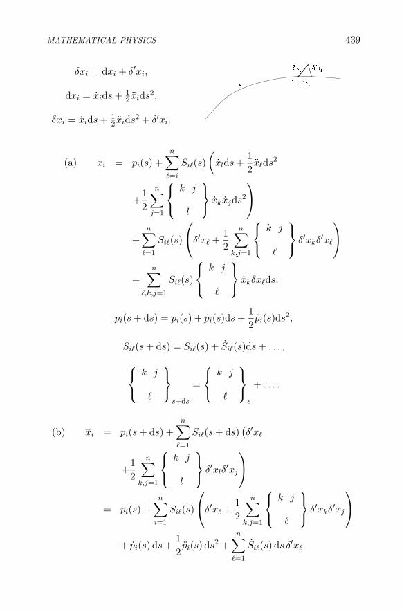
MATHEMATICAL PHYSICS 439

δxi = dxi + δ′xi,

dxi = xids + 12 xids2,

δxi = xids + 12 xids2 + δ′xi.

(a) xi = pi(s) +n∑

�=i

Si�(s)(

xlds +12x�ds2

+12

n∑

j=1

⎧⎨

⎩

k j

l

⎫⎬

⎭xkxjds2

⎞

⎠

+n∑

�=1

Si�(s)

⎛

⎝δ′x� +12

n∑

k,j=1

⎧⎨

⎩

k j

�

⎫⎬

⎭δ′xkδ

′x�

⎞

⎠

+n∑

�,k,j=1

Si�(s)

⎧⎨

⎩

k j

�

⎫⎬

⎭xkδx�ds.

pi(s + ds) = pi(s) + pi(s)ds +12pi(s)ds2,

Si�(s + ds) = Si�(s) + Si�(s)ds + . . . ,

⎧⎨

⎩

k j

�

⎫⎬

⎭s+ds

=

⎧⎨

⎩

k j

�

⎫⎬

⎭s

+ . . . .

(b) xi = pi(s + ds) +n∑

�=1

Si�(s + ds)(δ′x�

+12

n∑

k,j=1

⎧⎨

⎩

k j

l

⎫⎬

⎭δ′xlδ

′xj

⎞

⎠

= pi(s) +n∑

i=1

Si�(s)

⎛

⎝δ′x� +12

n∑

k,j=1

⎧⎨

⎩

k j

�

⎫⎬

⎭δ′xkδ

′xj

⎞

⎠

+ pi(s) ds +12pi(s) ds2 +

n∑

�=1

Si�(s) ds δ′x�.

440 E. MAJORANA: RESEARCH NOTES ON THEORETICAL PHYSICS

(a-b) pi(s) ds +12pi(s) ds2 +

n∑

�=1

Si�(s) ds δ′xl

=n∑

�=1

Si�(s)

⎛

⎝x�ds +12xlds2 +

12

n∑

k,j=1

⎧⎨

⎩

k j

�

⎫⎬

⎭xkxjds2

⎞

⎠

+n∑

�,k,j=1

Si�(s)

⎧⎨

⎩

k j

�

⎫⎬

⎭xkδ

′xj ds.

⎧⎪⎪⎪⎪⎪⎪⎪⎪⎪⎪⎪⎪⎪⎪⎪⎪⎪⎪⎨

⎪⎪⎪⎪⎪⎪⎪⎪⎪⎪⎪⎪⎪⎪⎪⎪⎪⎪⎩

1st order: pi(s) ds =n∑

�=1

Si�(s)x� ds,

2nd order:12pi(s),ds2 +

n∑

�=1

Si�(s)ds δ′xl

=12

n∑

�=1

Si�x�(s)ds2 +12

n∑

�,k,j=1

Si�(s)

⎧⎨

⎩

k j

�

⎫⎬

⎭xk xj ds2

+n∑

�,k,j=1

Si�(s)

⎧⎨

⎩

k j

�

⎫⎬

⎭xk δ′xj ds.

For arbitrary δ′xj :

⎧⎪⎪⎪⎪⎪⎪⎪⎪⎪⎪⎪⎪⎪⎪⎪⎪⎪⎪⎪⎪⎪⎨

⎪⎪⎪⎪⎪⎪⎪⎪⎪⎪⎪⎪⎪⎪⎪⎪⎪⎪⎪⎪⎪⎩

pi(s) =n∑

�=1

Si�(s)x� =n∑

j=1

Sij(s)xj (1)

(i = 1, 2, . . . , n),

pi(s) =n∑

�=1

Si�x�(s) +n∑

�,k,j=1

Si�(s)

⎧⎨

⎩

k j

�

⎫⎬

⎭xkxj (2)

(i = 1, 2, . . . , n),

Sij(s) =n∑

�,k=1

Si�(s)

⎧⎨

⎩

k j

�

⎫⎬

⎭xk (3)

(i, j = 1, 2, . . . , n).

From (3), by summing over every value of i, we obtain the quantities Sij

(with n2 arbitrary constants; for example they are given by the initial

MATHEMATICAL PHYSICS 441

values). By taking the derivative of (1) with respect to s and replacingSij(s) with their expression in (3), we get (2) identically. Then, it isenough to satisfy only (1). We find:

pi(s) =∫ n∑

�=1

Si�(s)x�(s)ds.

Since the integrals are defined up to a constant, we thus have 2n2 arbi-trary constants, n2 of which are trivial (additive constants). The finalformula coincides with the one already obtained above:

xi =∫ n∑

�=1

Si�x� ds +n∑

�=1

Si�

⎛

⎝δx� +n∑

k,j=1

⎧⎨

⎩

k j

�

⎫⎬

⎭δxkδxj

⎞

⎠

Si� being the solutions of the n differential systems (3).

9.6. RIEMANN’S SYMBOLS ANDPROPERTIES RELATING TOCURVATURE

9.6.1 Cyclic Displacement Round AnElementary Parallelogram

xi → xi + δxi → xi + δxi + δ′xi → xi + δ′xi → xi,

ui → uii → ui

2 → ui3 → ui

4.

dui = −n∑

k,j=1

⎧⎨

⎩

k j

i

⎫⎬

⎭ukdxj =

∑X i

jdxj ,

X ij = −

n∑

k=1

⎧⎨

⎩

k j

i

⎫⎬

⎭uk

(X ij is not a tensor). Up to 2nd order infinitesimals:

442 E. MAJORANA: RESEARCH NOTES ON THEORETICAL PHYSICS

δui = −n∑

k,j=1

⎧⎨

⎩

k j

i

⎫⎬

⎭0

(uk)0 δxj ,

X ij = −

n∑

k=1

⎧⎨

⎩

k j

i

⎫⎬

⎭0

(uk)0 −n∑

k,�=1

⎡

⎣ ∂

∂x�

⎧⎨

⎩

k j

i

⎫⎬

⎭

⎤

⎦

0

(ux)0 δx�

+n∑

k,�,m=1

⎧⎨

⎩

k j

i

⎫⎬

⎭0

⎧⎨

⎩

m �

k

⎫⎬

⎭0

(um)0 δx�.

Δui =∮ n∑

j=1

X ijdxj =

∫ P1

P

n∑

j=1

X ijdxj +

∫ P2

P1

. . . +∫ P3

P2

. . . +∫ P4=P

P3

. . .

=(∫ P1

P. . . +

∫ P3

P2

. . .

)+(∫ P2

P1

. . . +∫ P4=P

P3

. . .

)

=n∑

k,j,�=1

∂

∂x�

⎧⎨

⎩

k j

i

⎫⎬

⎭uk δx� dxj

−n∑

k,�,m,j=1

⎧⎨

⎩

k j

i

⎫⎬

⎭

⎧⎨

⎩

m �

k

⎫⎬

⎭um δx� dxj

−n∑

k,j,�=1

∂

∂x�

⎧⎨

⎩

k j

i

⎫⎬

⎭uk dx� δxj

+n∑

k,�,m,j=1

⎧⎨

⎩

k j

i

⎫⎬

⎭

⎧⎨

⎩

m �

k

⎫⎬

⎭um dx� δxj .

Δur = −n∑

i,h,k=1

ui dxk δxk

⎡

⎣n∑

p=1

⎛

⎝

⎧⎨

⎩

i k

p

⎫⎬

⎭

⎧⎨

⎩

p h

r

⎫⎬

⎭

−

⎧⎨

⎩

i h

p

⎫⎬

⎭

⎧⎨

⎩

p k

r

⎫⎬

⎭

+∂

∂xk

⎧⎨

⎩

i k

r

⎫⎬

⎭− ∂

∂xk

⎧⎨

⎩

i h

r

⎫⎬

⎭

⎞

⎠

⎤

⎦ .

MATHEMATICAL PHYSICS 443

Δur = +n∑

i,h,k=1

{ir, hk}ui dxh δxk

which is the Riemann curvature.

9.6.2 Fundamental Properties Of Riemann’SSymbols Of The Second Kind

{ir, hk} = − ∂

∂xh

⎧⎨

⎩

i k

r

⎫⎬

⎭+

∂

∂xk

⎧⎨

⎩

i h

r

⎫⎬

⎭

−n∑

p=1

⎡

⎣

⎧⎨

⎩

p h

r

⎫⎬

⎭

⎧⎨

⎩

i k

p

⎫⎬

⎭−

⎧⎨

⎩

p k

r

⎫⎬

⎭

⎧⎨

⎩

i h

p

⎫⎬

⎭

⎤

⎦

Properties of Riemann’s symbols of the second kind:

1) {ir, hk} = arihk,

(covariance with respect to the indices i, h, k,contravariance with respect to the index r)

2) {ir, hk} = −{ir, kh},

3) {ir, hk} + {hr, ki} + {kr, ih} = 0 .

Up to 2nd order infinitesimals:

{1 1, 1 2} =∂

∂x1

⎧⎨

⎩

1 2

1

⎫⎬

⎭− ∂

∂x2

⎧⎨

⎩

1 1

1

⎫⎬

⎭= 0,

{2 1, 1 2} =∂

∂x1

⎧⎨

⎩

2 2

1

⎫⎬

⎭− ∂

∂x2

⎧⎨

⎩

2 1

1

⎫⎬

⎭=

23

+13

= 1,

{1 2, 1 2} =∂

∂x1

⎧⎨

⎩

1 2

2

⎫⎬

⎭− ∂

∂x2

⎧⎨

⎩

1 1

2

⎫⎬

⎭= −1

3− 2

3= −1,

{2 2, 1 2} =∂

∂x1

⎧⎨

⎩

2 2

2

⎫⎬

⎭− ∂

∂x2

⎧⎨

⎩

2 1

2

⎫⎬

⎭= 0.

444 E. MAJORANA: RESEARCH NOTES ON THEORETICAL PHYSICS

Δur = −n∑

i,h,k=1

{ir, hk}uiδxh δ′xk.

[3]

r = 1 : Δu1 = −u2(δx1 δ′x2 − δx2 δ′x1),r = 2 : Δu2 = u1(δx1 δ′x2 − δx2 δ′x1).

9.6.3 Fundamental Properties And Number OfRiemann’s Symbols Of The First Kind

(ij, hk) =n∑

r=1

ajr{ir, hk}

= −n∑

r=1

ajr∂

∂xh

⎧⎨

⎩

i k

r

⎫⎬

⎭+

n∑

r=1

ajr∂

∂xk

⎧⎨

⎩

i h

r

⎫⎬

⎭

−n∑

p,r=1

ajr

⎡

⎣

⎧⎨

⎩

p h

r

⎫⎬

⎭

⎧⎨

⎩

i k

p

⎫⎬

⎭

−

⎧⎨

⎩

p k

r

⎫⎬

⎭

⎧⎨

⎩

i h

p

⎫⎬

⎭

⎤

⎦

= − ∂

∂xh

⎡

⎣i k

j

⎤

⎦+n∑

r=1

∂ajr

∂xh

⎧⎨

⎩

i k

r

⎫⎬

⎭

+∂

∂xk

⎡

⎣i h

j

⎤

⎦−n∑

r=1

∂ajr

∂xk

⎧⎨

⎩

i h

r

⎫⎬

⎭

−n∑

rp=1

⎛

⎝

⎡

⎣p h

j

⎤

⎦

⎧⎨

⎩

i k

p

⎫⎬

⎭−

⎡

⎣p k

j

⎤

⎦

⎧⎨

⎩

i h

p

⎫⎬

⎭

⎞

⎠ .

3@ In the original manuscript, the following note appears: Change the sign of Riemann’ssymbols. Also, the following is pointed out, referring to equations reported in Levi-Civita I:Notes on the Tallis formulae: Eq. (3), p.201 is correct; Eq. (4), p.201, change the sign; Eq.(26), p.219 is correct.

MATHEMATICAL PHYSICS 445

Since:

n∑

r=1

∂ajr

∂xh

⎧⎨

⎩

i k

r

⎫⎬

⎭=

n∑

p=1

⎡

⎣p h

j

⎤

⎦

⎧⎨

⎩

i k

p

⎫⎬

⎭+

n∑

p=1

⎡

⎣j h

p

⎤

⎦

⎧⎨

⎩

i k

p

⎫⎬

⎭

etc., we finally have:

(ij, hk) = − ∂

∂xh

⎡

⎣i k

j

⎤

⎦+∂

∂xk

⎡

⎣i h

j

⎤

⎦

+n∑

p=1

⎛

⎝

⎡

⎣j h

p

⎤

⎦

⎧⎨

⎩

i k

p

⎫⎬

⎭−

⎡

⎣j k

p

⎤

⎦+

⎧⎨

⎩

i h

p

⎫⎬

⎭

⎞

⎠ .

Properties of Riemann’s symbols of the first kind:

1) covariance with respect to every index,

2) (ij, hk) = −(ij, kh),

3) (ij, hk) = −(ji, hk).

In fact:

∂

∂xh

⎡

⎣i k

j

⎤

⎦− ∂

∂xk

⎡

⎣i h

j

⎤

⎦

=12

(∂2ajk

∂xi∂xh− ∂2aih

∂xi∂xk− prt2aik

∂xj∂xh+

∂2aih

∂xj∂xk

)

= −

⎛

⎝ ∂

∂xh

⎡

⎣j k

i

⎤

⎦− ∂

∂xk

⎡

⎣j h

i

⎤

⎦

⎞

⎠ ,

etc.;

n∑

p=1

⎡

⎣j h

p

⎤

⎦

⎧⎨

⎩

i k

p

⎫⎬

⎭=

n∑

p,q=1

apq

⎡

⎣j h

p

⎤

⎦

⎡

⎣i k

q

⎤

⎦

=n∑

p=1

⎡

⎣i k

p

⎤

⎦

⎧⎨

⎩

j h

p

⎫⎬

⎭,

446 E. MAJORANA: RESEARCH NOTES ON THEORETICAL PHYSICS

etc.

4) (ij, hk) + (hj, ki) + (kj, ih) = 0,

5) (ij, hk) + (ih, kj) + (ik, jh) = 0,

6) (ij, hk) = (hk, ij) .

In fact:

∂

∂xh

⎡

⎣i k

j

⎤

⎦− ∂

∂xk

⎡

⎣i h

j

⎤

⎦

=12

(∂2ajk

∂xi∂xh− ∂2aik

∂xj∂xh+

∂2ajh

∂xi∂xk+

∂2aih

∂xj∂xk

)

=∂

∂xi

⎡

⎣h j

k

⎤

⎦− ∂

∂xj

⎡

⎣h i

k

⎤

⎦

etc.; for the remaining proof, see property 3).

7) Number of the independent symbols of first kind.Given the indices i, j, h, k, irrespectively of their ordering, we have twoindependent symbols if all the indices are different from each other; oneindependent symbol if three indices are different and the fourth is equalto one of them; one independent symbol if we have two pairs of differentsymbols; no non-vanishing symbol in the other cases. Thus the totalnumber of independent symbols results to be:

2n(n − 1)(n − 2)(n − 3)

24+ 3

n(n − 1)(n − 2)6

+n(n − 1)

2

=n(n − 1)

12[(n − 2)(n − 3) + 6(n − 2) + 6] =

n2(n2 − 1)12

.

nn2(n2 − 1)

121 02 13 64 205 50

MATHEMATICAL PHYSICS 447

9.6.4 Bianchi Identity And Ricci LemmaThe Bianchi identity for the covariant derivatives of the Riemann’s sym-bols is:

{ir, hk}� + {ir, k�}h + {ir, �k}k = Arihk� = 0.

It can be easily verified by performing the covariant derivatives in locallycartesian coordinates.The same holds for the Ricci lemma:

(ij, hk)� + (ij, k�)h + (ij, �h)k = 0.

9.6.5 Tangent Geodesic Coordinates AroundThe Point P0

xi = (λi)0 s, xi =∫ s

0λids

(λi are evaluated in the point P0; in order to have geodesic coordinatesin P it is enough that the formula holds up to s2 terms, as we certainlyassume).

xi =n∑

k,j=1

⎧⎨

⎩

k j

i

⎫⎬

⎭xkxj = 0.

xi = −n∑

k,j=1

⎧⎨

⎩

k j

i

⎫⎬

⎭xkxj ,

...x i = −

n∑

k,j=1

ddxr

⎧⎨

⎩

k j

i

⎫⎬

⎭xkxj xr − 2

n∑

k,j=1

⎧⎨

⎩

k j

i

⎫⎬

⎭xkxj

= −n∑

k,j,r=1

d∂xr

⎧⎨

⎩

k j

i

⎫⎬

⎭xkxj xr

+ 2n∑

k,j,r,s=1

⎧⎨

⎩

k j

i

⎫⎬

⎭

⎧⎨

⎩

r s

j

⎫⎬

⎭xkxrxs.

448 E. MAJORANA: RESEARCH NOTES ON THEORETICAL PHYSICS

At a point P0:

xr = λr,

xr = −n∑

h,k=1

⎧⎨

⎩

h k

r

⎫⎬

⎭λhλk,

...x r =

n∑

i,h,k=1

xixhxk

⎡

⎣− ∂

∂xi

⎧⎨

⎩

h k

r

⎫⎬

⎭+ 2

n∑

p=1

⎧⎨

⎩

i p

r

⎫⎬

⎭

⎧⎨

⎩

h k

p

⎫⎬

⎭

⎤

⎦ .

INDEX

Acetylenevibration modes, 278

Actionfor the electromagnetic field, 57

Alkalis terms, 190polarization forces, 205

α particle, 364, 367Angular metric, 416Angular momentum

for the electromagnetic field, 78Associated vectors, 424, 428Atomic spectra

complex atoms, 219, 223hyperfine structure, 239hyperfine structures, 211

Atomic wavefunction, 136, 197, 201Atom

one-electronmagnetic moment, 229

Atomthree-electron

ground state, 183two-electron, 125, 133, 136

1s1s term, 1701s2s term, 1742p2s term, 1692s2p term, 155, 1582s2s term, 1692s terms, 144X term, 153, 159, 179Y ′ term, 153, 179energy levels, 144self-consistent field, 141

β particles traversing a medium, 368Bianchi identity, 447Bose-Einstein commutation relations, 94Center-of-mass, 347Christoffel’s symbols, 410–411Complete systems of differential operators,

406Compton effect, 331Coordinates

locally cartesian, 447Coulomb field, 318, 324

screening factor, 198Covariance index, 433Covariant differentiation, 428Cross section

two-electron scattering, 330Cunningham corrections to the Stokes’ law,

396Curie point, 299

Curl of a vector, 436Delta-function, 317Derivative

covariant, 428Determination of e, 390Determination of e/m, 387–388Deuterium, 363, 365Differential forms, 403Differential operators

complete systems, 406Jacobian systems, 407linear, 404

Dirac coordinates, 104, 339,Dirac equation, 25

16-component spinors, 484-component spinors, 475-component spinors, 556-component spinors, 48non-relativistic approximation, 242

Dirac fieldangular momentum, 40electromagnetic interaction, 25Hamiltonian, 46interacting with the electromagnetic field,

45normal mode decomposition, 31plane wave expansion, 44quantization, 22real, 35, 45

Dirac operatorsparticular representations, 32

Divergence of a tensor, 432Divergence of a vector, 431Electric charge (determination)

Millikan’s method, 396Thomson’s method, 395Townsend’s method, 394Wilson’s method, 396Zaliny’s method, 394

Electromagnetic and electrostatic mass, 397Electromagnetic field

analogy with the Dirac field, 59, 66Dirac formalism, 68Hamiltonian, 58interacting with bound electrons, 112interacting with electrons, 84Lagrangian, 57plane wave operators, 64quantization, 71, 78, 82, 84, 95, 100retarded, 116total energy, 58

Electron, 397bound, 112

449

450 E. MAJORANA: RESEARCH NOTES ON THEORETICAL PHYSICS

interaction with the electromagnetic field,84, 112

semiclassical theory, 4Electron wavefunction, 112Elliptic coordinates, 261Exchange energy, 223, 234, 290

tables, 204Exchange forces

nuclear, 340Extraction work, 398Fall velocity, 396Fermi-Dirac commutation relations, 94Ferromagnetism, 289, 300, 307Field extension, 435Gas

degenerate, 287, 352Gauge invariance, 30Geodesic coordinates, 425, 437

tangent, 447Geodesic curvature, 428Geodesic lines, 418, 428

autoparallelism, 424Geodesic manifolds, 436Geodesic surface, 437Goudsmith method, 213Ground state

three-electron atom, 183two-electron atom, 125

Hamiltonian formalism, 37, 43Helium

atomic wavefunction, 136composed of two deuterium nuclei, 340ionization energy, 128–129molecule, 261nuclear potential, 340

Houston formula, 213Hydrogen, 329Hydrogen atom, 327Hyperfine structures, 246, 251Ionization energy

for a two-electron atom, 129for a two electron atom, 128

Jacobian systems of differential operators,407

j-j coupling, 214Klein-Gordon equation, 7, 84, 370Lande formula, 211Langmuir experiment, 399Lithium, 201

electrostatic potential, 184ground state, 185

Lorentz transformationsfor the photon wavefunction, 70

Magnetic charges, 119Magnetic moment, 298

atomic, 247, 251for a one-electron atom, 229

nuclear, 247Magnetic moments

diagonal, 114Maxwell-Dirac theory, 29Maxwell distribution, 398Maxwell equations, 27

variational approach, 28Method of electrolysis (determination of e),

394Metric

indefinite, 425Millikan’s method (determination of e), 396Minimum approach distance, 324, 329Mobility coefficients, 394Molecules

vibration modes, 275Neutron-proton interaction, 340Neutron

susceptivity, 339wave equation, 339

Nuclear magnetic moment, 247Nuclear potential, 340Nuclei

scalar field theory, 370Nucleon density, 345Nucleon

interaction, 347, 352interaction potential, 340, 345kinetic energy, 345

Parallel displacement, 422Parallelism, 427

symbolic equations, 409Paramagnetism, 288Partial wave method, 319Pauli matrices, 3, 7Perturbation method

for a two-electron atom, 125, 157scattering, 316–317

Phase advancement, 323Photon

wave equation, 100Plane waves, 82Poisson brackets, 408Polarization forces, 205Potential

between nucleons, 340, 345nuclear, 340

Potential well, 311P ′ triplets, 233Quasi-stationary states, 332Radioactivity

tables, 339Radions, 293Reflecting power, 315Relativistic kinematics, 330–331Resonance

between � = 1 and �′ electrons, 223

INDEX 451

in the two-electron scattering, 330Retarded fields, 116Ricci lemma, 430, 447Richardson formula, 398Riemann curvature, 443Riemann’s symbols

first kind, 444second kind, 443

Russell-Saunders coupling, 214Rutherford formula, 324, 329Rydberg corrections, 212

relativistic, 239Saturation current, 392, 398Scattering

between two nuclei, 340Born method, 319bound electron, 112

coherent, 112Compton, 331Coulomb, 321, 328

Dirac method, 318Dirac method, 317free electron, 104from a potential well, 311intensity, 324, 329method of the particular solutions, 327quasi coulombian, 324resonant, 113screened Coulomb, 197simple perturbation method, 316transition probability, 318two-electron, 330

Schrodinger equation, 325, 329for a Coulomb field, 321

Screening factor, 198Slater determinants, 307Space charge, 399Spin-orbit coupling, 233Spin function, 108Stokes law, 396Surface waves, 385

Susceptibilityfor a one-electron atom, 229magnetic, 288

Susceptivityatomic, 209for the neutron, 339

Symmetrizationfor fermion fields, 35

Tallis formulae, 444Thermionic effect, 397Thomson formula

β particles, 368Thomson’s method (determination of e), 395Thomson’s method (determination of e/m),

387Three-fermion system, 282Time delay constant, 118Townsend coefficient

in air, 392Townsend effect, 390Townsend relation, 393Transformation laws

for covariant systems, 433Transition probability, 318Triplets P ′, 233Two-particle system

Dirac equation, 242ε systems, 434Variational method, 126

for a two-electron atom, 128Vector product, 435Vector

cyclic displacement, 441Vibrating string, 3Vibration modes in molecules, 275Wave equation

for the photon, 100Wavefunction

alkali atoms, 190two-electron atom, 133

Wien’s method (determination of e/m), 388Wilson’s method (determination of e), 396Zaliny’s method (determination of e), 394