Embed Size (px)
Citation preview
Volume 3 Number 10
Electronic Journal of Theoretical Physics
ISSN 1729-5254
EJTP
Majorana Issue
EditorIgnazio Licata
http://www.ejtp.com April, 2006 E-mail:[email protected]
Volume 3 Number 10
Electronic Journal of Theoretical Physics
ISSN 1729-5254
EJTP
Majorana Issue
EditorIgnazio Licata
http://www.ejtp.com April, 2006 E-mail:[email protected]

Editor in Chief
A. J. Sakaji
EJTP Publisher P. O. Box 48210 Abu Dhabi, UAE [email protected] [email protected]
Editorial Board
Co-Editor
Ignazio Licata,Foundations of Quantum Mechanics Complex System & Computation in Physics and Biology IxtuCyber for Complex Systems Sicily – Italy
[email protected]@ejtp.info [email protected]
Wai-ning Mei Condensed matter TheoryPhysics DepartmentUniversity of Nebraska at Omaha,
Omaha, Nebraska, USA e-mail: [email protected] [email protected]
Tepper L. Gill Mathematical Physics, Quantum Field Theory Department of Electrical and Computer Engineering Howard University, Washington, DC, USA e-mail: [email protected]
F.K. DiakonosStatistical Physics Physics Department, University of Athens Panepistimiopolis GR 5784 Zographos, Athens, Greece e-mail: [email protected]
Jorge A. Franco Rodríguez
General Theory of Relativity Av. Libertador Edificio Zulia P12 123 Caracas 1050 Venezuela e-mail: [email protected] [email protected]
J. A. MakiApplied Mathematics School of Mathematics University of East Anglia Norwich NR4 7TJ UK e-mail: [email protected]
Nicola Yordanov Physical Chemistry Bulgarian Academy of Sciences,BG-1113 Sofia, Bulgaria Telephone: (+359 2) 724917 , (+359 2) 9792546
e-mail: [email protected]
ndyepr[AT]bas.bg
S.I. ThemelisAtomic, Molecular & Optical Physics Foundation for Research and Technology - Hellas P.O. Box 1527, GR-711 10 Heraklion, Greece e-mail: [email protected]
T. A. HawaryMathematics Department of Mathematics Mu'tah University P.O.Box 6 Karak- Jordan e-mail: [email protected]
Arbab Ibrahim Theoretical Astrophysics and Cosmology Department of Physics, Faculty of Science, University of Khartoum, P.O. Box 321, Khartoum 11115, Sudan
e-mail: [email protected] [email protected]

Sergey Danilkin Instrument Scientist, The Bragg Institute Australian Nuclear Science and Technology Organization PMB 1, Menai NSW 2234 AustraliaTel: +61 2 9717 3338 Fax: +61 2 9717 3606
e-mail: [email protected]
Robert V. Gentry The Orion Foundation P. O. Box 12067 Knoxville, TN 37912-0067 USAe-mail: gentryrv[@orionfdn.org
Attilio Maccari Nonlinear phenomena, chaos and solitons in classic and quantum physics Technical Institute "G. Cardano" Via Alfredo Casella 3 00013 Mentana RM - ITALY
e-mail: [email protected]
Beny Neta Applied Mathematics Department of Mathematics Naval Postgraduate School 1141 Cunningham Road Monterey, CA 93943, USA
e-mail: [email protected]
Haret C. Rosu Advanced Materials Division Institute for Scientific and Technological Research (IPICyT) Camino a la Presa San José 2055 Col. Lomas 4a. sección, C.P. 78216 San Luis Potosí, San Luis Potosí, México
e-mail: [email protected]
A. AbdelkaderExperimental Physics Physics Department, AjmanUniversity Ajman-UAE e-mail: [email protected]
Leonardo Chiatti Medical Physics Laboratory ASL VT Via S. Lorenzo 101, 01100 Viterbo (Italy) Tel : (0039) 0761 236903 Fax (0039) 0761 237904
e-mail: [email protected]
Zdenek Stuchlik Relativistic Astrophysics Department of Physics, Faculty of Philosophy and Science, Silesian University, Bezru covo n´am. 13, 746 01 Opava, Czech Republic
e-mail: [email protected]
Copyright © 2003-2006 Electronic Journal of Theoretical Physics (EJTP) All rights reserved
Table of Contents
No Articles Page
1 Majorana Imoact on Contemporary Physics Ignazio Licata
i
2 The Scientific Work Of Ettore Majorana: An IntroductionErasmo Recami
1
3 On the Hamiltonian Form of Generalized Dirac Equation for Fermions with Two Mass States Sergey. I. Kruglov
11
4 Majorana Equation and exotics: Higher Derivative Models, Anyons and Noncommutative Geometry Mikhail S. Plyushchay
17
5 Wave Equations, Renormalization and Meaning of the Planck's Mass: Some Qualitative Considerations Leonardo Chiatti
33
6 Nonlinear Field Equations and Solitons as Particles Attilio Maccari
39
7 The Quantum Character of Physical Fields. Foundations of Field Theories Ludmila. I. Petrova
89
8 Relativistic Causality and Quasi -Orthomodular AlgebrasRenato Nobili
109
9 Lorentz Invariant Majorana Formulation of Electrodynamics in the Clifford Algebra Formalism Tomislav Ivezic
131
10 " Anticoherent" Spin States via the Majorana RepresentationJason Zimba
143
11 Stretching the Electron as Far as it Will Go G. W. Semenoff and P. Sodano
157
12 Why do Majorana Neutrinos Run Faster than Dirac Neutrinos?Zhi-zhong Xing and He Zhang
191
13 Universe Without Singularities A Group Approach to De Sitter Cosmology Ignazio Licata
211
14 Majorana and the Investigation of Infrared Spectra of Ammonia Elisabetta. Di Grezia
225
15 Exact Solution of Majorana Equation via Heaviside Operational Ansatz Valentino A. Simpao
239
16 A Logical Analysis of Majorana’s Papers on Theoretical Physics A. Drago and S. Esposito
249
17 Four Variations on Theoretical Physics by Ettore MajoranaSalvatore. Esposito
265
18 The Majorana Oscillator Eliano Pessa
285
19 Scattering of an \alpha Particle by a Radioactive NucleusUnpublished 1928 Ettore Majorana
293
20 Comments on a Paper by Majorana Concerning Elementary Particles David. M. Fradkin
305
Editorial Note
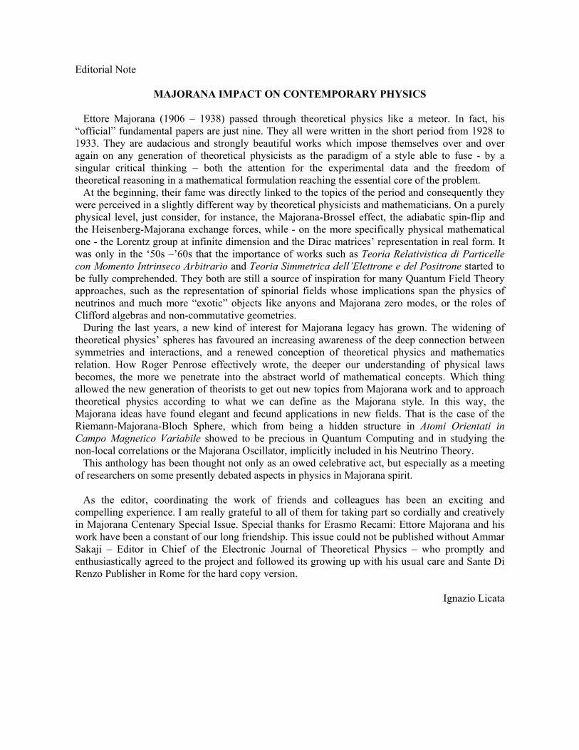
MAJORANA IMPACT ON CONTEMPORARY PHYSICS
Ettore Majorana (1906 – 1938) passed through theoretical physics like a meteor. In fact, his “official” fundamental papers are just nine. They all were written in the short period from 1928 to 1933. They are audacious and strongly beautiful works which impose themselves over and over again on any generation of theoretical physicists as the paradigm of a style able to fuse - by a singular critical thinking – both the attention for the experimental data and the freedom of theoretical reasoning in a mathematical formulation reaching the essential core of the problem.
At the beginning, their fame was directly linked to the topics of the period and consequently they were perceived in a slightly different way by theoretical physicists and mathematicians. On a purely physical level, just consider, for instance, the Majorana-Brossel effect, the adiabatic spin-flip and the Heisenberg-Majorana exchange forces, while - on the more specifically physical mathematical one - the Lorentz group at infinite dimension and the Dirac matrices’ representation in real form. It was only in the ‘50s –’60s that the importance of works such as Teoria Relativistica di Particelle con Momento Intrinseco Arbitrario and Teoria Simmetrica dell’Elettrone e del Positrone started to be fully comprehended. They both are still a source of inspiration for many Quantum Field Theory approaches, such as the representation of spinorial fields whose implications span the physics of neutrinos and much more “exotic” objects like anyons and Majorana zero modes, or the roles of Clifford algebras and non-commutative geometries.
During the last years, a new kind of interest for Majorana legacy has grown. The widening of theoretical physics’ spheres has favoured an increasing awareness of the deep connection between symmetries and interactions, and a renewed conception of theoretical physics and mathematics relation. How Roger Penrose effectively wrote, the deeper our understanding of physical laws becomes, the more we penetrate into the abstract world of mathematical concepts. Which thing allowed the new generation of theorists to get out new topics from Majorana work and to approach theoretical physics according to what we can define as the Majorana style. In this way, the Majorana ideas have found elegant and fecund applications in new fields. That is the case of the Riemann-Majorana-Bloch Sphere, which from being a hidden structure in Atomi Orientati in Campo Magnetico Variabile showed to be precious in Quantum Computing and in studying the non-local correlations or the Majorana Oscillator, implicitly included in his Neutrino Theory.
This anthology has been thought not only as an owed celebrative act, but especially as a meeting of researchers on some presently debated aspects in physics in Majorana spirit.
As the editor, coordinating the work of friends and colleagues has been an exciting and compelling experience. I am really grateful to all of them for taking part so cordially and creatively in Majorana Centenary Special Issue. Special thanks for Erasmo Recami: Ettore Majorana and his work have been a constant of our long friendship. This issue could not be published without Ammar Sakaji – Editor in Chief of the Electronic Journal of Theoretical Physics – who promptly and enthusiastically agreed to the project and followed its growing up with his usual care and Sante Di Renzo Publisher in Rome for the hard copy version.
Ignazio Licata
EJTP 3, No. 10 (2006) 1–10 Electronic Journal of Theoretical Physics
The Scientific Work Of Ettore Majorana:An Introduction
Erasmo Recami ∗
Facolta di Ingegneria, Universita statale di Bergamo; and I.N.F.N.–Sezione di Milano,Milan, Italia
Received 22 February 2006, Published 28 May 2006
Abstract: A Brief bibliography of the scientific work of Ettore Majorana has been discussed.c© Electronic Journal of Theoretical Physics. All rights reserved.
Keywords: Ettore Majorana, Scientific workPACS (2006): 01.30.Tt, 01.65.+g
1. Historical Prelude
Ettore Majorana’s fame solidly rests on testimonies like the following, from the
evocative pen of Giuseppe Cocconi. At the request of Edoardo Amaldi[1], he wrote from
CERN (July 18, 1965):
“In January 1938, after having just graduated, I was invited, essentially by you, to
come to the Institute of Physics at the University in Rome for six months as a teaching
assistant, and once I was there I would have the good fortune of joining Fermi, Bernardini
(who had been given a chair at Camerino a few months earlier) and Ageno (he, too, a
new graduate), in the research of the products of disintegration of μ “mesons” (at that
time called mesotrons or yukons), which are produced by cosmic rays [...]
“It was actually while I was staying with Fermi in the small laboratory on the second
floor, absorbed in our work, with Fermi working with a piece of Wilson’s chamber (which
would help to reveal mesons at the end of their range) on a lathe and me constructing a
jalopey for the illumination of the chamber, using the flash produced by the explosion of
an aluminum ribbon shortcircuited on a battery, that Ettore Majorana came in search of
Fermi. I was introduced to him and we exchanged few words. A dark face. And that was
2 Electronic Journal of Theoretical Physics 3, No. 10 (2006) 1–10
it. An easily forgettable experience if, after a few weeks while I was still with Fermi in
that same workshop, news of Ettore Majorana’s disappearance in Naples had not arrived.
I remember that Fermi busied himself with telephoning around until, after some days, he
had the impression that Ettore would never be found.
“It was then that Fermi, trying to make me understand the significance of this loss,
expressed himself in quite a peculiar way; he who was so objectively harsh when judging
people. And so, at this point, I would like to repeat his words, just as I can still hear
them ringing in my memory: ‘Because, you see, in the world there are various categories
of scientists: people of a secondary or tertiary standing, who do their best but do not
go very far. There are also those of high standing, who come to discoveries of great
importance, fundamental for the development of science’ (and here I had the impression
that he placed himself in that category). ‘But then there are geniuses like Galileo and
Newton. Well, Ettore was one of them. Majorana had what no one else in the world had
[...]’”
And, with first-hand knowledge, Bruno Pontecorvo, adds: “Some time after his entry
into Fermi’s group, Majorana already possessed such an erudition and had reached such
a high level of comprehension of physics that he was able to speak on the same level with
Fermi about scientific problems. Fermi himself held him to be the greatest theoretical
physicist of our time. He often was astounded [...]. I remember exactly these words that
Fermi spoke: ‘If a problem has already been proposed, no one in the world can resolve it
better than Majorana.’ ” (See also [2].)
Ettore Majorana disappeared rather misteriously on March 26, 1938, and was never
seen again [3]. The myth of his “disappearance” has contributed to nothing more than
the notoriety he was entitled to, for being a true genius and a genius well ahead of his
time.
Majorana was such a pioneer, that even his manuscripts known as the Volumetti,
which comprise his study notes written in Rome between 1927, when he abandoned his
studies in engineering to take up physics, and 1931, are a paragon not only of order,
based on argument and even supplied with an index, but also of conciseness, essentiality
and originality: So much so that those notebooks could be regarded as an excellent
modern text of theoretical physics, even after about eighty years, and a “gold-mine” of
seminal new theoretical, physical, and mathematical ideas and hints, quite stimulating
and useful for modern research. Such scientific manuscripts, incidentally, have been
published for the first time (in 2003) by Kluwer[4]. But Majorana’s most interesting
notebooks or papers –those that constituted his “reserach notes” will not see the light in
the near future: it being too hard the task of selecting, interpreting and...electronically
typing them! Each notebook was written during a period of about one year, starting
from the years —as we said above— during which Ettore Majorana was completing
his studies at the University of Rome. Thus the contents of these notebooks range
from typical topics covered in academic courses to topics at the frontiers of research.
Despite this unevenness in the level of sophistication, the style in which any particular
Electronic Journal of Theoretical Physics 3, No. 10 (2006) 1–10 3
topic is treated is never obvious. As an example, we refer here to Majorana’s study
of the shift in the melting point of a substance when it is placed in a magnetic field
or, more interestingly, his examination of heat propagation using the “cricket simile.”
Also remarkable is his treatment of contemporary physics topics in an original and lucid
manner, such as Fermi’s explanation of the electromagnetic mass of the electron, the
Dirac equation with its applications, and the Lorentz group, revealing in some cases
the literature preferred by him. As far as frontier research arguments are concerned,
let us here recall only two illuminating examples: the study of quasi-stationary states,
anticipating Fano’s theory by about 20 years, and Fermi’s theory of atoms, reporting
analytic solutions of the Thomas-Fermi equation with appropriate boundary conditions
in terms of simple quadratures, which to our knowledge were still lacking.
Let us recall that Majorana, after having switched to physics at the beginning of
1928, graduated with Fermi on July 6, 1929, and went on to colaborate with the famous
group created by Enrico Fermi and Franco Rasetti (at the start with O.M.Corbino’s
important help); a theoretical subdivision of which was formed mainly (in the order of
their entrance into the Institute) by Ettore Majorana, Gian Carlo Wick, Giulio Racah,
Giovanni Gentile Jr., Ugo Fano, Bruno Ferretti, and Piero Caldirola. The members of
the experimental subgroup were: Emilio Segre, Edoardo Amaldi, Bruno Pontecorvo, Eu-
genio Fubini, Mario Ageno, Giuseppe Cocconi, along with the chemist Oscar D’Agostino.
Afterwards, Majorana qualified for university teaching of theoretical physics (“Libera
Docenza”) on November 12, 1932; spent about six months in Leipzig with W. Heisenberg
during 1933; and then, for some unknown reasons, stopped participating in the activities
of Fermi’s group. He even ceased publishing the results of his research, except for his
paper “Teoria simmetrica dell’elettrone e del positrone,” which (ready since 1933) Majo-
rana was persuaded by his colleagues to remove from a drawer and publish just prior to
the 1937 Italian national competition for three full-professorships.
With respect to the last point, let us recall that in 1937 there were numerous Italian
competitors for these posts, and many of them were of exceptional caliber; above all:
Ettore Majorana, Giulio Racah, Gian Carlo Wick, and Giovanni Gentile Jr. (the son of
the famous philosopher bearing the same name, and the inventor of “parastatistics” in
quantum mechanics). The judging committee was chaired by E. Fermi and had as mem-
bers E. Persico, G. Polvani, A. Carrelli, and O. Lazzarino. On the recommendation of the
judging committee, the Italian Minister of National Education installed Majorana as pro-
fessor of theoretical physics at Naples University because of his “great and well-deserved
fame,” independently of the competition itself; actually, “the Commission hesitated to
apply the normal university competition procedures to him.” The attached report on the
scientific activities of Ettore Majorana, sent to the minister by the committee, stated:
“Without listing his works, all of which are highly notable both for their originality
of the methods utilized as well as for the importance of the achieved results, we limit
ourselves to the following:
“In modern nuclear theories, the contribution made by this researcher to the introduc-
4 Electronic Journal of Theoretical Physics 3, No. 10 (2006) 1–10
tion of the forces called “Majorana forces” is universally recognized as the one, among the
most fundamental, that permits us to theoretically comprehend the reasons for nuclear
stability. The work of Majorana today serves as a basis for the most important research
in this field.
“In atomic physics, the merit of having resolved some of the most intricate questions
on the structure of spectra through simple and elegant considerations of symmetry is due
to Majorana.
“Lastly, he devised a brilliant method that permits us to treat the positive and neg-
ative electron in a symmetrical way, finally eliminating the necessity to rely on the ex-
tremely artificial and unsatisfactory hypothesis of an infinitely large electrical charge
diffused in space, a question that had been tackled in vain by many other scholars.”
One of the most important works of Ettore Majorana, the one that introduces his
“infinite-components equation” was not mentioned, since it had not yet been understood.
It is interesting to note, however, that the proper light was shed on his theory of electron
and anti-electron symmetry (today climaxing in its application to neutrinos and anti-
neutrinos) and on his resulting ability to eliminate the hypothesis known as the “Dirac
sea,” a hypothesis that was defined as “extremely artificial and unsatisfactory,” despite
the fact that in general it had been uncritically accepted.
The details of Majorana and Fermi’s first meeting were narrated by E. Segre [5]:
“The first important work written by Fermi in Rome [‘Su alcune proprieta statistiche
dell’atomo’ (On certain statistical properties of the atom)] is today known as the Thomas-
Fermi method. . . . When Fermi found that he needed the solution to a non-linear differ-
ential equation characterized by unusual boundary conditions in order to proceed, in a
week of assiduous work with his usual energy, he calculated the solution with a little hand
calculator. Majorana, who had entered the Institute just a short time earlier and who
was always very skeptical, decided that Fermi’s numeric solution probably was wrong and
that it would have been better to verify it. He went home, transformed Fermi’s original
equation into a Riccati equation, and resolved it without the aid of any calculator, utiliz-
ing his extraordinary aptitude for numeric calculation. When he returned to the Institute
and skeptically compared the little piece of paper on which he had written his results
to Fermi’s notebook, and found that their results coincided exactly, he could not hide
his amazement.” We have indulged in the foregoing anecdote since the pages on which
Majorana solved Fermi’s differential equation have in the end been found, and it has been
shown recently [6] that he actually followed two independent (and quite original) paths
to the same mathematical result, one of them leading to an Abel, rather than a Riccati,
equation.
Majorana delivered his lectures only during the beginning of 1938, starting on Jan.13
and ending with his disappearance (March 26). But his activity was intense, and his
interest for teaching extremely high. For the benefit of his beloved students, and perhaps
also for writinng down a book, he prepared careful notes for his lectures. And ten of
such lectures appeared in print in 1987 (see ref.[7]): and arised the admired comments of
Electronic Journal of Theoretical Physics 3, No. 10 (2006) 1–10 5
many (especially British) scholars. The remainig six lecture-notes, which had gone lost,
have been rediscovered in 2005 by Salvatore Esposito and Antonino Drago, and will soon
appear in print.
2. Ettore Majorana’s Published Papers
Majorana published few scientific articles: nine, actually, besides his sociology paper
entitled “Il valore delle leggi statistiche nella fisica e nelle scienze sociali” (The value of
statistical laws in physics and the social sciences), which was however published not by
Majorana but (posthumously) by G. Gentile Jr., in Scientia [36 (1942) 55-56]. We already
know that Majorana switched from engineering to physics in 1928 (the year in which he
published his first article, written in collaboration with his friend Gentile) and then went
on to publish his works in theoretical physics only for a very few years, practically only
until 1933. Nevertheless, even his published works are a mine of ideas and techniques of
theoretical physics that still remains partially unexplored. Let us list his nine published
articles:
(1) “Sullo sdoppiamento dei termini Roentgen ottici a causa dell’elettrone rotante e
sulla intensita delle righe del Cesio,” in collaboration with Giovanni Gentile Jr.,
Rendiconti Accademia Lincei 8 (1928) 229-233.
(2) “Sulla formazione dello ione molecolare di He,” Nuovo Cimento 8 (1931) 22-28.
(3) “I presunti termini anomali dell’Elio,” Nuovo Cimento 8 (1931) 78-83.
(4) “Reazione pseudopolare fra atomi di Idrogeno,” Rendiconti Accademia Lincei 13
(1931) 58-61.
(5) “Teoria dei tripletti P’ incompleti,” Nuovo Cimento 8 (1931) 107-113.
(6) “Atomi orientati in campo magnetico variabile,” Nuovo Cimento 9 (1932) 43-50.
(7) “Teoria relativistica di particelle con momento intrinseco arbitrario,” Nuovo Cimento
9 (1932) 335-344.
(8) “Uber die Kerntheorie,” Zeitschrift fur Physik 82 (1933) 137-145; and “Sulla teoria
dei nuclei,” La Ricerca Scientifica 4(1) (1933) 559-565.
(9) “Teoria simmetrica dell’elettrone e del positrone,” Nuovo Cimento 14 (1937) 171-
184.
The first papers, written between 1928 and 1931, concern atomic and molecular
physics: mainly questions of atomic spectroscopy or chemical bonds (within quantum
mechanics, of course). As E. Amaldi has written [1], an in-depth examination of these
works leaves one struck by their superb quality: They reveal both a deep knowledge of
the experimental data, even in the minutest detail, and an uncommon ease, without equal
at that time, in the use of the symmetry properties of the quantum states in order to
qualitatively simplify problems and choose the most suitable method for their quantita-
tive resolution. Among the first papers, “Atomi orientati in campo magnetico variabile”
(Atoms oriented in a variable magnetic field) deserves special mention. It is in this arti-
6 Electronic Journal of Theoretical Physics 3, No. 10 (2006) 1–10
cle, famous among atomic physicists, that the effect now known as the Majorana-Brossel
effect is introduced. In it, Majorana predicts and calculates the modification of the spec-
tral line shape due to an oscillating magnetic field. This work has also remained a classic
in the treatment of non-adiabatic spin-flip. Its results —once generalized, as suggested
by Majorana himself, by Rabi in 1937 and by Bloch and Rabi in 1945— established the
theoretical basis for the experimental method used to reverse the spin also of neutrons
by a radio-frequency field, a method that is still practiced today, for example, in all
polarized-neutron spectrometers. The Majorana paper introduces moreover the so-called
Majorana sphere (to represent spinors by a set of points on the surface of a sphere), as
noted not long ago by R. Penrose [8] and others.
Majorana’s last three articles are all of such importance that none of them can be set
aside without comment.
The article “Teoria relativistica di particelle con momento intrinseco arbitrario” (Rel-
ativistic theory of particles with arbitrary spin) is a typical example of a work that is so
far ahead of its time that it became understood and evaluated in depth only many years
later. Around 1932 it was commonly thought that one could write relativistic quantum
equations only in the case of particles with zero or half spin. Convinced of the contrary,
Majorana —as we know from his manuscripts— began constructing suitable quantum-
relativistic equations [9] for higher spin values (one, three-halves, etc.); and he even
devised a method for writing the equation for a generic spin-value. But still he published
nothing, until he discovered that one could write a single equation to cover an infinite
series of cases, that is, an entire infinite family of particles of arbitrary spin (even if at
that time the known particles could be counted on one hand). In order to implement his
programme with these “infinite components” equations, Majorana invented a technique
for the representation of a group several years before Eugene Wigner did. And, what is
more, Majorana obtained the infinite-dimensional unitary representations of the Lorentz
group that will be re-discovered by Wigner in his 1939 and 1948 works. The entire theory
was re-invented by Soviet mathematicians (in particular Gelfand and collaborators) in a
series of articles from 1948 to 1958 and finally applied by physicists years later. Sadly,
Majorana’s initial article remained in the shadows for a good 34 years until D. Fradkin,
informed by E. Amaldi, released [Am. J. Phys. 34 (1966) 314] what Majorana many
years earlier had accomplished.
As soon as the news of the Joliot-Curie experiments reached Rome at the beginning
of 1932, Majorana understood that they had discovered the “neutral proton” without
having realized it. Thus, even before the official announcement of the discovery of the
neutron, made soon afterwards by Chadwick, Majorana was able to explain the structure
and stability of atomic nuclei with the help of protons and neutrons, antedating in this
way also the pioneering work of D. Ivanenko, as both Segre and Amaldi have recounted.
Majorana’s colleagues remember that even before Easter he had concluded that protons
and neutrons (indistinguishable with respect to the nuclear interaction) were bound by the
Electronic Journal of Theoretical Physics 3, No. 10 (2006) 1–10 7
“exchange forces” originating from the exchange of their spatial positions alone (and not
also of their spins, as Heisenberg would propose), so as to produce the alpha particle (and
not the deuteron) saturated with respect to the binding energy. Only after Heisenberg
had published his own article on the same problem was Fermi able to persuade Majorana
to meet his famous colleague in Leipzig; and finally Heisenberg was able to convince
Majorana to publish his results in the paper “Uber die Kerntheorie.” Majorana’s paper
on the stability of nuclei was immediately recognized by the scientific community –a
rare event, as we know, from his writings– thanks to that timely “propaganda” made by
Heisenberg himself. We seize the present opportunity to quote two brief passages from
Majorana’s letters from Leipzig. On February 14, 1933, he writes his mother (the italics
are ours): “The environment of the physics institute is very nice. I have good relations
with Heisenberg, with Hund, and with everyone else. I am writing some articles in
German. The first one is already ready....” The work that is already ready is, naturally,
the cited one on nuclear forces, which, however, remained the only paper in German.
Again, in a letter dated February 18, he tells his father (we italicize): “I will publish
in German, after having extended it, also my latest article which appeared in Nuovo
Cimento.” Actually, Majorana published nothing more, either in Germany or after his
return to Italy, except for the article (in 1937) of which we are about to speak. It is
therefore of importance to know that Majorana was engaged in writing other papers: in
particular, he was expanding his article about the infinite-components equations.
As we said, from the existing manuscripts it appears that Majorana was also formu-
lating the essential lines of his symmetric theory of electrons and anti-electrons during the
years 1932-1933, even though he published this theory only years later, when participating
in the forementioned competition for a professorship, under the title “Teoria simmetrica
dell’elettrone e del positrone” (Symmetrical theory of the electron and positron), a pub-
lication that was initially noted almost exclusively for having introduced the Majorana
representation of the Dirac matrices in real form. A consequence of this theory is that a
neutral fermion has to be identical with its anti-particle, and Majorana suggested that
neutrinos could be particles of this type. As with Majorana’s other writings, this article
also started to gain prominence only decades later, beginning in 1957; and nowadays
expressions like Majorana spinors, Majorana mass, and Majorana neutrinos are fashion-
able. As already mentioned, Majorana’s publications (still little known, despite it all) is
a potential gold-mine for physics. Recently, for example, C. Becchi pointed out how, in
the first pages of the present paper, a clear formulation of the quantum action princi-
ple appears, the same principle that in later years, through Schwinger’s and Symanzik’s
works, for example, has brought about quite important advances in quantum field theory.
3. Ettore Majorana’s Unpublished Papers
Majorana also left us several unpublished scientific manuscripts, all of which have
been catalogued [10] and kept at the “Domus Galilaeana” of Pisa, Italy. Our analysis
8 Electronic Journal of Theoretical Physics 3, No. 10 (2006) 1–10
of these manuscripts has allowed us to ascertain that all the existing material seems to
have been written by 1933; even the rough copy of his last article, which Majorana pro-
ceeded to publish in 1937 —as already mentioned— seems to have been ready by 1933,
the year in which the discovery of the positron was confirmed. Indeed, we are unaware
of what he did in the following years from 1934 to 1938, except for a series of 34 letters
written by Majorana between March 17, 1931, and November 16, 1937, in reply to his
uncle Quirino —a renowned experimental physicist and at a time president of the Ital-
ian Physical Society— who had been pressing Majorana for theoretical explanations of
his own experiments. By contrast, his sister Maria recalled that, even in those years,
Majorana —who had reduced his visits to Fermi’s Institute, starting from the beginning
of 1934 (that is, after his return from Leipzig)— continued to study and work at home
many hours during the day and at night. Did he continue to dedicate himself to physics?
From a letter of his to Quirino, dated January 16, 1936, we find a first answer, because
we get to learn that Majorana had been occupied “since some time, with quantum elec-
trodynamics”; knowing Majorana’s modesty and love for understatements, this no doubt
means that by 1935 Majorana had profoundly dedicated himself to original research in
the field of quantum electrodynamics.
Do any other unpublished scientific manuscripts of Majorana exist? The question,
raised by his letters from Leipzig to his family, becomes of greater importance when
one reads also his letters addressed to the National Research Council of Italy (CNR)
during that period. In the first one (dated January 21, 1933), Majorana asserts: “At the
moment, I am occupied with the elaboration of a theory for the description of arbitrary-
spin particles that I began in Italy and of which I gave a summary notice in Nuovo
Cimento....” In the second one (dated March 3, 1933) he even declares, referring to
the same work: “I have sent an article on nuclear theory to Zeitschrift fur Physik. I
have the manuscript of a new theory on elementary particles ready, and will send it
to the same journal in a few days.” Considering that the article described here as a
“summary notice” of a new theory was already of a very high level, one can imagine how
interesting it would be to discover a copy of its final version, which went unpublished. [Is
it still, perhaps, in the Zeitschrift fur Physik archives? Our own search ended in failure].
One must moreover not forget that the above-cited letter to Quirino Majorana, dated
January 16, 1936, revealed that his nephew continued to work on theoretical physics even
subsequently, occupying himself in depth, at least, with quantum electrodynamics.
Some of Majorana’s other ideas, when they did not remain concealed in his own mind,
have survived in the memories of his colleagues. One such reminiscence we owe to Gian
Carlo Wick. Writing from Pisa on October 16, 1978, he recalls: “...The scientific contact
[between Ettore and me], mentioned by Segre, happened in Rome on the occasion of
the ‘A. Volta Congress’ (long before Majorana’s sojourn in Leipzig). The conversation
took place in Heitler’s company at a restaurant, and therefore without a blackboard...;
but even in the absence of details, what Majorana described in words was a ‘relativistic
theory of charged particles of zero spin based on the idea of field quantization’ (second
Electronic Journal of Theoretical Physics 3, No. 10 (2006) 1–10 9
quantization). When much later I saw Pauli and Weisskopf’s article [Helv. Phys. Acta 7
(1934) 709], I remained absolutely convinced that what Majorana had discussed was the
same thing....”
We attach to this paper a short bibliography. Far from being exhaustive, it provides
only some references about the topics touched upon in this Introduction.
Acknowledgments
The author wishes to thank Ignazio Licata for his kind invitation to contribute to
this book. He is moreover grateful to A. van der Merwe, Salvatore Esposito and Ettore
Majoranna Jr. for their very stimulating cooperation along the years; and acknowledges
useful discussions with many colleagues (in particular Dharam Ahluwalia, Roberto Bat-
tiston and Enrico Giannetto).
10 Electronic Journal of Theoretical Physics 3, No. 10 (2006) 1–10
References
[1] E.Amaldi, La Vita e l’Opera di E. Majorana (Accademia dei Lincei; Rome, 1966);“Ettore Majorana: Man and scientist,” in Strong and Weak Interactions. Presentproblems, A.Zichichi ed. (Academic; New York, 1966).
[2] B.Pontecorvo, Fermi e la fisica moderna (Editori Riuniti; Rome, 1972); and inProceedings International Conference on the History of Particle Physics, Paris, July1982, Physique 43 (1982).
[3] E.Recami: Il caso Majorana: Epistolario, Documenti, Testimonianze, 2nd edition(Oscar, Mondadori; Milan, 1991), pp.230; 4th edition (Di Renzo; Rome, 2002), pp.273.
[4] S.Esposito, E.Majorana Jr., A. van der Merwe and E.Recami (editors): EttoreMajorana — Notes on Theoretical Pysics (Kluwer Acad. Press; Dordrecht and Boston,2003); 512 pages.
[5] E.Segre: Enrico Fermi, Fisico (Zanichelli; Bologna (1971); and Autobiografia di unFisico (Il Mulino; Rome, 1995).
[6] S.Esposito: “Majorana solution of the Thomas-Fermi equation”, Am. J. Phys. 70(2002) 852-856; “Majorana transformation for differential equations”, Int. J. Theor.Phys. 41 (2002) 2417-2426.
[7] Ettore Majorana – Lezioni all’Universita di Napoli, ed. by B.Preziosi (Bibliopolis;Napoli, 1987).
[8] R.Penrose, “Newton, quantum theory and reality,” in 300 Years of Gravitation,S.W.Hawking and W.Israel eds. (University Press; Cambridge, 1987); J.Zimba andR.Penrose, Stud. Hist. Phil. Sci. 24 (1993) 697; R. Penrose: Ombre della Mente(Shadows of the Mind) (Rizzoli; 1996), pp.338–343 and 371–375; and subsequent papersby C.Leonardi, F.Lillo, et al.
[9] R.Mignani, E.Recami e M.Baldo: “About a Dirac–like equation for the photon,according to E.Majorana”, Lett. Nuovo Cimento 11 (1974) 568, and subsequent papersby E.Giannetto and by S.Esposito.
[10] M.Baldo, R.Mignani, and E.Recami, “Catalogo dei manoscritti scientifici inediti diE.Majorana,” in Ettore Majorana – Lezioni all’Universita di Napoli, B.Preziosi ed.(Bibliopolis; Naples, 1987) pp.175-197; and E.Recami, “Ettore Majorana: L’opera editaed inedita,” Quaderni di Storia della Fisica (of the Giornale di Fisica) (S.I.F., Bologna)5 (1999) 19-68.
EJTP 3, No. 10 (2006) 11–16 Electronic Journal of Theoretical Physics
On the Hamiltonian Form of Generalized DiracEquation for Fermions with Two Mass States
S. I. Kruglov ∗
Physical and Environmental Sciences Department,University of Toronto at Scarborough,
1265 Military Trail, Toronto, Ontario, Canada M1C 1A4
Received 18 March 2006, Published 28 May 2006
Abstract: Dynamical and non-dynamical components of the 20-component wave function areseparated in the generalized Dirac equation of the first order, describing fermions with spin1/2 and two mass states. After the exclusion of the non-dynamical components, we obtainthe Hamiltonian Form of equations. Minimal and non-minimal electromagnetic interactions ofparticles are considered here.c© Electronic Journal of Theoretical Physics. All rights reserved.
Keywords: Quantum Electrodynamics, Dirac Equation, Barut Equation, ElectromagneticInteraction of ParticlesPACS (2006): 12.20.-m,03.65.Pm,94.20.wj
1. Introduction
We continue to investigate the first order generalized Dirac equation (FOGDE),
describing fermions with spin 1/2 and two mass states. This 20-component wave equation
was obtained in [1] on the base of Barut’s [2] second order equation describing particles
with two mass states. Barut suggested the second order wave equation for the unified
description of e, μ leptons. He treated this equation as an effective equation for partly
“dressed” fermions using the non-perturbative approach to quantum electrodynamics.
Some investigations of Barut’s second order wave equation and FOGDE were performed
in [3], [4], [5], [6], [7].
The purpose of this paper is to obtain the Hamiltonian Form of the 20-component
wave equation of the first order.
The paper is organized as follows. In Sec. 2, we introduce the generalized Dirac
12 Electronic Journal of Theoretical Physics 3, No. 10 (2006) 11–16
equation of the first order. The dynamical and non-dynamical components of the 20-
component wave function are separated, and quantum-mechanical Hamiltonian is derived
in Sec. 3. In Sec. 4, we make a conclusion. In Appendix, we give some useful matrices
entering the Hamiltonian. The system of units � = c = 1 is chosen, Latin letters run 1,
2, 3, and Greek letters run 1, 2, 3, 4, and notations as in [8] are used.
2. Field Equation of the First Order
The Barut second order field equation describing spin-1/2 and two mass states of
particles may be rewritten as [1]:(γμ∂μ − a
m∂2
μ + m)
ψ(x) = 0, (1)
where ∂μ = ∂/∂xμ = (∂/∂xm, ∂/∂(it)), ψ(x) is a Dirac spinor, m is a parameter with
the dimension of the mass, and a is a massless parameter. We imply a summation over
repeated indices. The commutation relations γμγν + γνγμ = 2δμν are valid for the Dirac
matrices. Masses of fermions are given by
m1 = ±m
(1−√4a + 1
2a
), m2 = ±m
(1 +√
4a + 1
2a
). (2)
Signs in Eq. (2) should be chosen to have positive values of m1, m2.
Eq. (1) can be represented in the first order form [1]:
(αμ∂μ + m) Ψ(x) = 0, (3)
where the 20-dimensional wave function Ψ(x) and 20× 20-matrices αμ are
Ψ(x) = {ψA(x)} =
⎛⎜⎝ ψ(x)
ψμ(x)
⎞⎟⎠ (ψμ(x) = − 1
m∂μψ(x)), (4)
αμ =(εμ,0 + aε0,μ
)⊗ I4 + ε0,0 ⊗ γμ. (5)
The I4 is a unit 4× 4-matrix, and ⊗ is a direct product of matrices. The elements of the
entire algebra obey equations as follows (see, for example, [9]):(εM,N
)AB
= δMAδNB, εM,AεB,N = δABεM,N , (6)
where A,B, M, N = 0, 1, 2, 3, 4.
After introducing the minimal electromagnetic interaction by the substitution ∂μ →Dμ = ∂μ − ieAμ (Aμ is the four-vector potential of the electromagnetic field), and the
non-minimal interaction with the electromagnetic field by adding two parameters κ1, κ2,
we come [1] to the matrix equation:[αμDμ +
i
2(κ0P0 + κ1P1) αμνFμν + m
]Ψ(x) = 0, (7)
Electronic Journal of Theoretical Physics 3, No. 10 (2006) 11–16 13
where P0 = ε0,0 ⊗ I4, P1 = εμ,μ ⊗ I4 are the projection operators, P 20 = P0, P 2
1 = P1,
P0 + P1 = 1, and αμν = αμαν − αναμ. Parameters κ0 and κ1 characterize fermion
anomalous electromagnetic interactions.
The tensor form of Eq. (7) is given by
(γνDν + iκ0γμγνFμν + m) ψ(x) + (aDμ + iκ0γνFνμ) ψμ(x) = 0, (8)
(Dμ + iκ1γνFμν) ψ(x) + (mδμν + iκ1aFμν) ψν(x) = 0, (9)
where Fμν = ∂μAν − ∂νAμ is the strength of the electromagnetic field. Eq. (8), (9) rep-
resent the system of equations for Dirac spinor ψ(x) and vector-spinor ψν(x) interacting
with electromagnetic fields.
3. Quantum-Mechanical Hamiltonian
In order to obtain the quantum-mechanical Hamiltonian, we rewrite Eq. (7) as
follows:
iα4∂tΨ(x) =
[αaDa + m + eA0α4+
(10)
+i
2(κ0P0 + κ1P1) αμνFμν
]Ψ(x).
One can verify with the help of Eq. (6) that the matrix α4 obeys the matrix equation
α44 − (1 + 2a)α2
4 + a2Λ = 0, (11)
where Λ:
Λ =(ε0,0 + ε4,4
)⊗ I4, (12)
is the projection operator, Λ2 = Λ. It should be noted that the matrix Λ can be considered
as the unit matrix in the 8-dimensional sub-space of the wave function [1]. The operator
Λ, acting on the wave function Ψ(x), extracts the dynamical components Φ(x) = ΛΨ(x).
We may separate1 the dynamical and non-dynamical components of the wave function
Ψ(x) by introducing the second projection operator:
Π = 1− Λ = εm,m ⊗ I4, (13)
so that Π2 = Π. This operator defines non-dynamical components Ω = ΠΨ(x). Multi-
plying Eq. (10) by the matrix
(1 + 2a)
a2α4 − α3
4
a2=
(ε0,4 +
1
aε4,0
)⊗ I4 − 1
aε4,4 ⊗ γ4,
and taking into consideration Eq. (11), we obtain the equation as follows:
i∂tΦ(x) = eA0Φ(x) +
[(1 + 2a)
a2α4 − α3
4
a2
] [αaDa + m + K
]Ψ(x), (14)
1 In the work [1], the dynamical and non-dynamical components of the wave function were not separated.
14 Electronic Journal of Theoretical Physics 3, No. 10 (2006) 11–16
where
K =i
2(κ0P0 + κ1P1) αμνFμν
(15)
= iFμν
[κ0
(ε0,0 ⊗ γμγν + ε0,ν ⊗ γμ
)+ κ1
(εμ,0 ⊗ γν + aεμ,ν ⊗ I4
)].
It should be mentioned that because Λ+Π = 1, the equality Ψ(x) = Φ(x)+Ω(x) is valid.
To eliminate the non-dynamical components Ω(x) from Eq. (14), we multiply Eq. (10)
by the matrix Π, and using the equality Πα4 = 0, we obtain
Π (αaDa + K) (Φ(x) + Ω(x)) + mΩ(x) = 0. (16)
With the help of equation ΠαaΠ = 0, one may find from Eq. (16), the expression as
follows:
Ω(x) = − (m + ΠK)−1 Π (αaDa + K) Φ(x). (17)
With the aid of Eq. (17), Eq. (14) takes the form
i∂tΦ(x) = HΦ(x), (18)
H = eA0 +
[(1 + 2a)
a2α4 − α3
4
a2
] [αaDa + m + K
](19)
× [1− (m + ΠK)−1 Π (αbDb + K)],
Eq. (18) represents the Hamiltonian form of the equation for 8-component wave function
Φ(x). It is obvious that for the relativistic description of fermionic fields, possessing two
mass states, it is necessary to have 8-component wave function (two bispinors). The
Hamiltonian (19) can be simplified by using products of matrices given in Appendix.
Now we consider the particular case of fermions minimally interacting with electro-
magnetic fields, κ0 = κ1 = 0, K = 0. In this case, Eq. (18) becomes
i∂tΦ(x) =
[eA0 +
m
a
(aε0,4 ⊗ I4 + ε4,0 ⊗ I4 − ε4,4 ⊗ γ4
)(20)
+1
a
(ε4,0 ⊗ γm
)Dm − 1
m
(ε4,0 ⊗ I4
)D2
m
]Φ(x).
In component form, Eq. (20) is given by the system of equations
i∂tψ(x) = eA0ψ(x) + mψ4(x),
(21)
i∂tψ4(x) =(eA0 − m
aγ4
)ψ4(x) +
(m
a+
1
aγmDm − 1
mD2
m
)ψ(x).
Eq. (21) can also be obtained from Eq. (8), (9), at κ0 = κ1 = 0, after the exclusion of
non-dynamical (auxiliary) components ψm(x) = −(1/m)Dmψ(x). So, only components
with time derivatives enter Eq. (21) and Eq. (18).
Electronic Journal of Theoretical Physics 3, No. 10 (2006) 11–16 15
4. Conclusion
We have analyzed the 20-component matrix equation of the first order, describing
fermions with spin 1/2 and two mass states which is convenient for different applications.
There are two parameters characterizing non-minimal electromagnetic interactions of
fermions including the interaction of the anomalous magnetic moment of particles. The
Hamiltonian form of the equation was obtained, and it was shown that the wave func-
tion, entering the Hamiltonian equation, contains 8 components what is necessary for
describing fermionic field with two mass states in the formalism of the first order. The
Hamiltonian (19) can be used for a consideration of the non-relativistic limit which is
convenient for the physical interpretation of constants κ0, κ1 introduced. This can be
done with the help of the Foldy - Wouthuysen procedure [10].
The approach developed may be applied for a consideration of two families of leptons
or quarks, but this requires further investigations.
Appendix
With the help of Eq. (6), one can obtain expressions as follows:[(1 + 2a)
a2α4 − α3
4
a2
]αmDm =
(1
aε4,0 ⊗ γm + ε4,m ⊗ I4
)Dm, (22)
ΠαmDm =(εm,0 ⊗ I4
)Dm, (23)
ΠK = iκ1Fmν
(εm,0 ⊗ γν + aεm,ν ⊗ I4
), (24)[
(1 + 2a)
a2α4 − α3
4
a2
]K = i
κ0
aFμν
(ε4,0 ⊗ γμγν + ε4,ν ⊗ γμ
)(25)
+iκ1F4ν
(ε0,0 ⊗ γν − 1
aε4,0 ⊗ γ4γν + aε0,ν ⊗ I4 − ε4,ν ⊗ γ4
).
One may verify that the equations
FnmFmi = BnBi −B2δni, FnmFmiFik = −B2Fnk (26)
are hold, where B2 = B2m, Bm = (1/2)εmnkFnk is the strength of the magnetic field. Eq.
(26) allow us to obtain the relation for the matrix Σ ≡ m + ΠK:
Σ4 − 4mΣ3 +(6m2 − b
)Σ2 + 2m
(b− 2m2
)Σ + m4 − bm2 = 0, (27)
where b = a2κ21B
2. From Eq. (27), we find the inverse matrix Σ−1:
Σ−1 =1
m2 (b−m2)
[Σ3 − 4mΣ2 +
(6m2 − b
)Σ + 2m
(b− 2m2
)]=
1
m+
1
m2 (b−m2)
[iκ1
(m2 − b
)Fmν + amκ21FmkFkν (28)
−ia2κ31FmkFknFnν
] (εm,0 ⊗ γν + aεm,ν ⊗ I4
).
16 Electronic Journal of Theoretical Physics 3, No. 10 (2006) 11–16
References
[1] S. I. Kruglov, Ann. Fond. Broglie 29, 1005 (2004); Errata-ibid (in press); arXiv:quant-ph/0408056.
[2] A. O. Barut, Phys. Lett. 73B, 310 (1978); Phys. Rev. Lett. 42, 1251 (1979).
[3] A. O. Barut, P. Cordero, and G. C. Ghirardi, Nuovo. Cim. A66, 36 (1970).
[4] A. O. Barut, P. Cordero, and G. C. Ghirardi, Phys. Rev. 182, 1844 (1969).
[5] R. Wilson, Nucl. Phys. B68, 157 (1974).
[6] V. V. Dvoeglazov, Int. J. Theor. Phys. 37, 1009 (1998); Ann. Fond. Broglie 25, 81(2000); Hadronic J. 26, 299 (2003).
[7] S. I. Kruglov, Quantization of fermionic fields with two mass states in the first orderformalism, to appear in the proceedings of 18th Workshop on Hadronic MechanicsHonoring the 70th Birthday of Prof. R.M. Santilli (Karlstad, Sweden, 20-22 Jun2005); arXiv: hep-ph/0510103.
[8] A. I. Ahieser, and V. B. Berestetskii, Quantum Electrodynamics (New York: WileyInterscience, 1969).
[9] S.I.Kruglov, Symmetry and Electromagnetic Interaction of Fields with Multi-Spin(Nova Science Publishers, Huntington, New York, 2001).
[10] L.L. Foldy, and S. A. Wouthuysen, Phys. Rev. 78, 29 (1950).
EJTP 3, No. 10 (2006) 17–31 Electronic Journal of Theoretical Physics
Majorana Equation and Exotics: Higher DerivativeModels, Anyons and Noncommutative Geometry
Mikhail S. Plyushchay ∗
Departamento de Fısica, Universidad de Santiago de Chile,Casilla 307, Santiago 2, Chile
Received 20 April 2006, Published 28 May 2006
Abstract: In 1932 Ettore Majorana proposed an infinite-component relativistic wave equationfor particles of arbitrary integer and half-integer spin. In the late 80s and early 90s it wasfound that the higher-derivative geometric particle models underlie the Majorana equation,and that its (2+1)-dimensional analogue provides with a natural basis for the description ofrelativistic anyons. We review these aspects and discuss the relationship of the equation to theexotic planar Galilei symmetry and noncommutative geometry. We also point out the relationof some Abelian gauge field theories with Chern-Simons terms to the Landau problem in thenoncommutative plane from the perspective of the Majorana equation.c© Electronic Journal of Theoretical Physics. All rights reserved.
Keywords: Majorana Equation, Dirac Equation, Noncommutative Geometry, Gauge TheoriesPACS (2006): 02.40.Gh, 03.65.Pm, 11.15.-q, 11.15.Ex
1. Introduction
Ettore Majorana was the first to study the infinite-component relativistic fields. In
the pioneering 1932 paper [1], on the basis of the linear differential wave equation of a
Dirac form, he constructed a relativistically invariant theory for arbitrary integer or half-
integer spin particles. It was the first recognition, development and application of the
infinite-dimensional unitary representations of the Lorentz group. During a long period
of time, however, the Majorana results remained practically unknown, and the theory
was rediscovered in 1948 by Gel’fand and Yaglom [2] in a more general framework of the
group theory representations. In 1966 Fradkin revived the Majorana remarkable work
(on the suggestion of Amaldi) by translating it into English and placing it in the context
of the later research [3]. In a few years the development of the concept of the infinite-
18 Electronic Journal of Theoretical Physics 3, No. 10 (2006) 17–31
component fields [4]–[8] culminated in the construction of the dual resonance models and
the origin of the superstring theory [9]–[15].
After the revival, the Majorana work inspired an interesting line of research based
on a peculiar property of his equation: its time-like solutions describe positive energy
states lying on a Regge type trajectory, but with unusual dependence of the mass, M ,
on the spin, s, Ms ∝ (const + s)−1. In 1970, Dirac [16] proposed a covariant spinor set
of linear differential equations for the infinite-component field, from which the Majorana
and Klein-Gordon equations appear in the form of integrability (consistency) conditions.
As a result, the new Dirac relativistic equation describes a massive, spin-zero positive-
energy particle. Though this line of research [17]–[22] did not find essential development,
in particular, due to the problems arising under the attempt to introduce electromagnetic
interaction, recently it was pushed [23]–[25] in the unexpected direction related to the
anyon theory [26]–[38], exotic Galilei symmetry [39]–[42], and non-commutative geometry
[43]–[46].
In pseudoclassical relativistic particle model associated with the quantum Dirac spin-
1/2 equation, the spin degrees of freedom are described by the odd Grassmann variables
[47]. In 1988 it was observed [48] that the (3+1)D particle analogue of the Polyakov
string with rigidity [49] possesses the mass spectrum of the squared Majorana equation.
The model of the particle with rigidity contains, like the string model [49], the higher
derivative curvature term in the action. It is this higher derivative term that effectively
supplies the system with the even spin degrees of freedom of noncompact nature and leads
to the infinite-dimensional representations of the Lorentz group. Soon it was found that
the quantum theory of another higher derivative model of the (2+1)D relativistic particle
with torsion [32], whose Euclidean version underlies the Bose-Fermi transmutation mech-
anism [50], is described by the linear differential infinite-component wave equation of the
Majorana form. Unlike the original Majorana equation, its (2+1)D analogue provides
with the quantum states of any (real) value of the spin, and so, can serve as a basis for
the construction of relativistic anyon theory [31]–[38]. It was shown recently [23, 24] that
the application of the special non-relativistic limit (c → ∞, s → ∞, s/c2 → κ = const)
[51, 52] to the model of relativistic particle with torsion produces the higher derivative
model of a planar particle [40] with associated exotic (two-fold centrally extended) Galilei
symmetry [39]. The quantum spectrum of the higher derivative model [40], being un-
bounded from below, is described by reducible representations of the exotic planar Galilei
group. On the other hand, the application of the same limit to the (2+1)D analogue of the
Dirac spinor set of anyon equations [38] gives rise to the Majorana-Dirac-Levy-Leblond
type infinite-component wave equations [24], which describe irreducible representations
of the exotic planar Galilei group corresponding to a free particle with non-commuting
coordinates [41].
Here we review the described relations of the Majorana equation to the higher deriva-
tive particle models, exotic Galilei symmetry and associated noncommutative structure.
We also discuss the relationship of the (2+1)D relativistic Abelian gauge field theories
with Chern-Simons terms [55]–[62] to the Landau problem in the noncommutative plane
Electronic Journal of Theoretical Physics 3, No. 10 (2006) 17–31 19
[25, 41, 53, 54] from the perspective of the Majorana equation.
2. Majorana Equation and Dirac Spinor Set of Equations
Majorana equation [1] is a linear differential equation of the Dirac form,
(P μΓμ −m) Ψ(x) = 0, (2.1)
with P μ = i∂μ and matrices Γμ generating the Lorentz group via the anti-de Sitter
SO(3,2) commutation relations similar to those satisfied by the usual γ-matrices1,
[Γμ, Γν ] = iSμν , [Sμν , Γλ] = i(ηνλΓμ − ημλΓν), (2.2)
[Sμν , Sλρ] = i(ημρSνλ − ημλSνρ + ηνλSμρ − ηνρSμλ). (2.3)
The original Majorana realization of the Γμ corresponds to the infinite-dimensional uni-
tary representation of the Lorentz group in which its Casimir operators C1 and C2 and
the Lorentz scalar ΓμΓμ take the values
C1 ≡ 1
2SμνS
μν = −3
4, C2 ≡ εμνλρSμνSλρ = 0, ΓμΓμ = −1
2. (2.4)
A representation space corresponding to (2.4) is a direct sum of the two irreducible
SL(2,C) representations characterized by the integer, j = 0, 1, . . ., and half-integer, j =
1/2, 3/2, . . ., values of the SU(2) subalgebra Casimir operator, M2i = j(j + 1), Mi ≡
12εijkS
jk. In both cases the Majorana equation (2.1) has time-like (massive), space-like
(tachyonic) and light-like (massless) solutions. The spectrum in the light-like sector is
Mj =m
j + 12
, j = s + n, n = 0, 1, . . . , s = 0 or1
2. (2.5)
The change Γμ → −Γμ in accordance with (2.2), (2.3) does not effect on representations
of the Lorentz group as a subgroup of the SO(3,2). For the Majorana choice with the
diagonal generator Γ0,
Γ0 = j +1
2, (2.6)
Eq. (2.1) has the time-like (P 2 < 0) solutions with positive energy.
In [16], Dirac suggested an interesting modification of the Majorana infinite-component
theory that effectively singles out the lowest spin zero time-like state from all the Majo-
rana equation spectrum. The key idea was to generate the Klein-Gordon and Majorana
wave equations via the integrability conditions for some covariant set of linear differential
equations. Dirac covariant spinor set of (3+1)D equations has the form
DaΨ(x, q) = 0, Da = (P μγμ + m)abQb, (2.7)
1 We use the metric with signature (−,+, +, +).
20 Electronic Journal of Theoretical Physics 3, No. 10 (2006) 17–31
where γ-matrices are taken in the Majorana representation, and Qa = (q1, q2, π1, π2) is
composed from the mutually commuting dynamical variables qα, α = 1, 2, and commuting
conjugate momenta πα, [qα, πβ] = iδαβ, while Ψ(x, q) is a single-component wave function.
The SO(3,2) generators are realized here as quadratic in Q operators,
Γμ =1
4QγμQ, Sμν =
i
8Q[γμ, γν ]Q,
where Q = Qtγ0. The covariance of the set of equations (2.7) follows from the com-
mutation relations [Sμν , Q] = − i4[γμ, γν ]Q, which mean that the Qa is transformed as a
Lorentz spinor, and so, the set of four equations (2.7) is the spinor set. Note also that
[Γμ, Q] = 12γμQ, and the Qa anticommute between themselves for a linear combination of
the SO(3,2) generators. This means that the Qa, Γμ and Sμν generate a supersymmetric
extension of the anti-de Sitter algebra.
The Klein-Gordon,
(P 2 + m2)Ψ = 0, (2.8)
and the Majorana equations (with the parameter m changed in the latter for 12m) are
the integrability conditions for the spinor set of equations (2.7) [16]. Taking into account
that the Γ0 = 14(q2
1 + q22 + π2
1 + π22) coincides up to the factor 1
2with the Hamiltonian of a
planar isotropic oscillator, one finds that the possible eigenvalues of the Γ0 are given by
the sets j = 0, 1, . . . and j = 1/2, 3/2, . . . in correspondence with Eq. (2.6). The former
case corresponds to the Γ0 eigenstates given by the even in qα wave functions, while the
latter case corresponds to the odd eigenstates. Having in mind the Majorana equation
spectrum (2.5) (with the indicated change of the mass parameter) and Eq. (2.8), one
concludes that the spinor set of equations (2.7) describes the positive energy spinless
states2 of the fixed mass.
3. Higher Derivative Relativistic Particle Models
The model of relativistic particle with curvature [48, 63, 64, 65], being an analogue
of the model of relativistic string with rigidity [49], is given by the reparametrization
invariant action
A = −∫
(m + αk)ds, (3.1)
where ds2 = −dxμdxμ, α > 0 is a dimensionless parameter3, and k is the worldline
curvature, k2 = x′′μx
′′μ, x′μ = dxμ/ds. In a parametrization xμ = xμ(τ), Lagrangian of the
system is L = −√−x2(m+k), where we assume that the particle moves with the velocity
less than the speed of light, x2 < 0, xμ = dxμ/dτ , and then k2 = (x2x2−(xx2)2)/(x2)3 ≥ 0
2 Staunton [20] proposed a modification of the Dirac spinor set of equations that describes the spin-1/2representation of the Poincare group3 For α < 0 the equations of motion of the system have the only solutions corresponding to the curvature-free case α = 0 of a spinless particle of mass m [48].
Electronic Journal of Theoretical Physics 3, No. 10 (2006) 17–31 21
[48]. The Lagrangian equations of motion have the form of the conservation law of the
energy-momentum vector,
d
dτPμ = 0, Pμ =
∂L
∂xμ− d
dτ
(∂L
∂xμ
). (3.2)
The dependence of the Lagrangian on higher derivatives supplies effectively the system
with additional translation invariant degrees of freedom described by the velocity vμ ≡ xμ
and conjugate momentum [48]. This higher derivative dependence is responsible for a
peculiarity of the system: though the particle velocity is less than the speed of light, the
equations of motion (3.2) have the time-like (P 2 < 0), the light-like (P 2 = 0) and the
space-like (P 2 > 0) solutions [48], whose explicit form was given in [48, 65]. This indicates
on a possible relation of the model (3.1) to the infinite-component field theory associated
with the Majorana equation. Unlike the Majorana system, however, the quantum version
of the model (3.1) has the states of integer spin only, which lie on the nonlinear Regge
trajectory of the form very similar to (2.5) [48],
Ml =m√
1 + α−2l(l + 1), l = 0, 1, . . . . (3.3)
The choice of the laboratory time gauge τ = x0 separates here the positive energy time-
like solutions.
Before we pass over to the discussion of a relativistic particle model more closely
related to the original (3+1)D Majorana equation from the viewpoint of the structure of
the spectrum, but essentially different from it in some important properties, it is worth
to note that the higher derivative dependence of the action does not obligatorily lead to
the tachyonic states. In Ref. [66] the model given by the action of the form (3.1) with
parameter m = 0 was suggested. It was shown there that in the case of x2 < 0, the
model is inconsistent (its equations of the motion have no solutions), but for x2 > 0 the
model is consistent and describes massless states of the arbitrary, but fixed integer or
half-integer helicities λ = ±j, whose values are defined by the quantized parameter α,
α2 = j2. The velocity higher than the speed of light in such a model originates from the
Zittervewegung associated with nontrivial helicity. System (3.1) with m = 0 possesses
additional local symmetry [66, 67] (action (3.1) in this case has no scale parameter), and
it is such a gauge symmetry that is responsible for separation of the two physical helicity
components from the infinite-component Majorana type field (cf. the system given by
the Dirac spinor set of equations (2.7)). Recently, the interest to such a higher derivative
massless particle system has been revived [68, 69] in the context of the massless higher
spin field theories [70, 71].
The (2+1)D relativistic model of the particle with torsion [32] is given by the action
A = −∫
(m + α�)ds, � = εμνλx′μx
′′νx
′′′λ , (3.4)
where α is a dimensionless parameter, and � is the particle worldline trajectory torsion.
Unlike the model (3.1), here the parameter α can take positive or negative values, and for
22 Electronic Journal of Theoretical Physics 3, No. 10 (2006) 17–31
the sake of definiteness, we assume that α > 0. Action (3.4) with α = 1/2 appeared origi-
nally in the Euclidean version in the context of the Bose-Fermi transmutation mechanism
[50, 29]. Like the model of the particle with curvature (3.1), the higher derivative system
(3.4) possesses the translation invariant dynamical spin degrees of freedom Jμ = −αeμ,
eμ = xμ/√−x2, as well as the three types of solutions to the classical equations of motion,
with P 2 < 0, P 2 = 0 and P 2 > 0 [32]. At the quantum level operators Jμ satisfy the
SO(2,1) commutation relations
[Jμ, Jμ] = −iεμνλJλ, (3.5)
analogous to those for the (2+1)D γ-matrices. Note that in (2+1)D, there is a duality
relation Jμ = −12εμνλS
νλ between the (2+1)D vector Jμ and the spin tensor Sμν satisfying
the commutation relations of the form (2.3). The parameter α is not quantized here, and
it fixes the value of the Casimir operator of the algebra (3.5), J2 = −α(α − 1) [32]. For
the gauge τ = x0, in representation where the operator J0 is diagonal, its eigenvalues
are j0 = α + n, n = 0, 1, . . .. This means that the spin degrees of freedom of the
system realize a bounded from below unitary infinite-dimensional representation D+α of
the universal covering group of the (2+1)D Lorentz group [72, 73]. The physical states
of the system are given by the quantum analogue of the constraint responsible for the
reparametrization invariance of the action (3.4) [32],
(PJ − αm)Ψ = 0. (3.6)
One can treat Eq. (3.6) as a (2+1)D analogue of the original Majorana equation (2.1).
The difference of the (2+1)D from the (3+1)D case proceeds from the isomorphism be-
tween SO(2,2) and SO(2,1)⊕SO(2,1) algebras, and here the SO(2,1) generators Jμ simul-
taneously play the role analogous to that played by the SO(3,2) generators Γμ satisfying
the commutation relations (2.2). In the time-like sector, the solutions of Eq. (3.6) de-
scribe the positive energy states of the spin sn = α + n lying on the Majorana type
trajectory [32]
Mn =m
1 + α−1n, n = 0, 1, . . . . (3.7)
4. Fractional Spin Fields
The (2+1)D analogue of the Majorana equation (3.6) being supplied with the Klein-
Gordon equation (2.8) describes the fields carrying irreducible representation of the
Poincare ISO(2,1) group of any, but fixed spin s = α > 0 [32], and so, can serve as a basis
for relativistic anyon theory [26]–[31]. Instead of these two equations, one can obtain the
same result starting from the linear differential (2+1)D Majorana-Dirac wave equations
suggested in [34]4. In such a case it is supposed that besides the index n associated with
the infinite-dimensional half-bounded unitary representation D+α , the infinite-component
4 Jackiw and Nair [33] proposed an alternative theory based on the (2+1)D Majorana equation suppliedwith the equation for topologically massive vector gauge field.
Electronic Journal of Theoretical Physics 3, No. 10 (2006) 17–31 23
field carries in addition a spinor index, and that it satisfies Eq. (3.6) as well as the Dirac
equation
(Pγ −m)Ψ = 0. (4.1)
As a consequence of Eqs. (3.6), (4.1), the Majorana-Dirac field satisfies not only the
Klein-Gordon equation, but also the equations
(Jγ + α)Ψ = 0, εμνλJμγνP λΨ = 0, (4.2)
and one finds that it describes the positive energy states of the mass m and spin s = α− 12
[34].
The alternative way to describe an anyon field of the fixed mass and spin consists in the
construction of the (2+1)D analogue of the Dirac spinor set of equations (2.7) generating
the Majorana and Klein-Gordon equations in the form of integrability conditions. The
construction needs the application of the so called deformed Heisenberg algebra with
reflection intimately related to parabosons [74, 75],
[a−, a+] = 1 + νR, R2 = 1, {a±, R} = 0, (4.3)
where ν is a real deformation parameter. Here operator N = 12{a+, a−} − 1
2(ν + 1) plays
the role of a number operator, [N, a±] = ±a±, allowing us to present a reflection operator
R in terms of a±: R = (−1)N = cos πN . For ν > −1 algebra (4.3) admits infinite-
dimensional unitary representations realized on a Fock space5. In terms of operators a±
the SO(2,1) generators (3.5) are realized in a quadratic form,
J0 =1
4{a+, a−}, J± = J1 ± iJ2 =
1
2(a±)2. (4.4)
Here JμJμ = −s(s−1) with s = 1
4(1±ν) on the even/odd eigensubspaces of the reflection
operator R, i.e. as in the (3+1)D case we have a direct sum of the two infinite-dimensional
irreducible representations of the (2+1)D Lorentz group. These quadratic operators
together with linear operators
L1 =1√2(a+ + a−), L2 =
i√2(a+ − a−), (4.5)
extend the SO(2,1) algebra into the OSP(1|2) superalgebra:
{Lα, Lβ} = 4i(Jγ)αβ, [Jμ, Lα] =1
2(γμL)α, (4.6)
where the (2+1)D γ-matrices are taken in the Majorana representation, (γ0)αβ = (σ2)α
β,
(γ1)αβ = i(σ1)α
β, (γ2)αβ = i(σ3)α
β, and (γμ)αβ = (γμ)αρερβ. With these ingredients, the
(2+1)D analogue of the Dirac spinor set of wave equations (2.7) is [38]((Pγ)α
β + mεαβ)LβΨ = 0. (4.7)
5 For negative odd integer values ν = −(2k + 1), k = 1, 2 . . ., the algebra has finite, (2k+1)-dimensionalnonunitary representations [74].
24 Electronic Journal of Theoretical Physics 3, No. 10 (2006) 17–31
From these two (α = 1, 2) equations the (2+1)D Majorana and Klein-Gordon equations
appear in the form of integrability conditions.
The spinor set of equations (4.7) was used, in particular, for investigation of the
Lorentz symmetry breaking in the (3+1)D massless theories with fractional helicity states
[76].
5. Exotic Galilei Group and Noncommutative Plane
A special non-relativistic limit (c is a speed of light) [51, 52]
c→∞, s→∞,s
c2= κ, (5.1)
applied to the spinor set of equations (4.7) results in the infinite-component Dirac-
Majorana-Levy-Leblond type wave equations [24]
i∂tφk +
√k + 1
2θ
P+
mφk+1 = 0, (5.2)
P−φk +
√2(k + 1)
θφk+1 = 0, (5.3)
where k = 0, 1, . . ., P± = P1 ± iP2, and
θ =κ
m2. (5.4)
The first equation (5.2) defines the dynamics. The second equation relates different
components of the field allowing us to present them in terms of the lowest component,
φk = (−1)k(κ
2
) k2
(P−m
)k
φ0. (5.5)
Though a simple substitution of the second equation into the first one shows that every
component φk satisfies the Shrodinger equation of a free planar particle, the nontrivial
nature of the system is encoded in its symmetry. The (2+1)D Poincare symmetry of the
original relativistic system in the limit (5.1) is transformed into the exotic planar Galilei
symmetry characterized by the noncommutative boosts [39, 41],
[K1,K2] = −iκ. (5.6)
The system of the two infinite-component equations (5.2), (5.3) can be presented in the
equivalent form
i∂tφ = Hφ, V−φ = 0, (5.7)
with
H = Pivi − 1
2mv+v− , V− = v− − P−
m. (5.8)
The translation invariant operators v± = v1±iv2, [vi, vj] = −iκ−1εij, is the non-relativistic
limit (5.1) of the noncompact Lorentz generators, −(c/s)J± → v±. The symmetry of the
Electronic Journal of Theoretical Physics 3, No. 10 (2006) 17–31 25
quantum mechanical system (5.7) is given by the Hamiltonian H, the space translation
generators Pi, and by the rotation and boost generators,
J = εijxiPj +1
2κv+v−, Ki = mxi − tPi + κεijvj. (5.9)
These integrals generate the algebra of the two-fold centrally extended planar Galilei
group [39, 41] characterized by the non-commutativity of the boosts (5.6).
The first equation from (5.7) is nothing else as a non-relativistic limit of the (2+1)D
Majorana equation (3.6) [24]. The system described by it (without the second equation
from (5.7)) corresponds to the classical system given by the higher derivative Lagrangian
L =1
2mxi
2 + κεijxixj, (5.10)
which, in its turn, corresponds to the non-relativistic limit (5.1) of the relativistic model
of the particle with torsion (3.4) [23]. It is interesting to note that the system (5.10) (for
the first time considered by Lukierski, Stichel and Zakrzewski [40], in ignorance of its
relation to the relativistic higher derivative model (3.4)), reveals the same dynamics as
a charged non-relativistic planar particle in external homogeneous magnetic and electric
fields [77]. The spectrum of the Hamiltonian (5.8),
En(P ) =1
2mP 2
i −mκ−1n, n = 0, 1, . . . , (5.11)
is not restricted from below, and the system (5.10), similarly to its relativistic analogue
(3.4), describes a reducible representation of the exotic Galilei group. The role of the
second equation from (5.7), whose component form is given by Eq. (5.3), consists in
singling out the highest (at fixed P 2i ) energy state from (5.11) with n = 0, and fixing an
irreducible infinite-dimensional unitary representation of the exotic planar Galilei group
[24, 77]. The system being reduced to the surface given by this second equation (classically
equivalent to the set of the two second class constraints Vi = 0, i = 1, 2) corresponds to
the exotic planar particle considered by Duval and Horvathy [41, 79], which is described
by the free particle Hamiltonian and an exotic symplectic two-form,
H =1
2mP 2
i , ω = dPi ∧ dxi +1
2θεijdPi ∧ dPj. (5.12)
The system (5.12) reveals a noncommutative structure encoded in the nontrivial commu-
tation relations of the particle coordinates,
[xi, xj] = iθεij. (5.13)
This noncommutative structure is the non-relativistic limit (5.1) [51] of the commutation
relations
[xμ, xν ] = −isεμνλP λ
(−P 2)3/2(5.14)
associated with the minimal canonical approach for relativistic anyon of spin s [78]. Note
that as was observed by Schonfeld [55] (see also [80]), the commutation relations (5.14) are
26 Electronic Journal of Theoretical Physics 3, No. 10 (2006) 17–31
dual to the (Euclidean) commutation relations for the mechanical momentum of a charged
particle in the magnetic monopole field. The latter system also admits a description by
the higher derivative Lagrangian [80],
LCM =1
2m�r 2 − eg
|�r|(�r × �r)2
(�r × �r) · �r . (5.15)
There is a close relationship between the charge-monopole non-relativistic system (5.15)
and the model of relativistic particle with torsion (3.4). Indeed, in a parametrization xμ =
xμ(τ), the torsion term from (3.4) takes the (Minkowski) form of the higher derivative
charge-monopole coupling term, but in the velocity space with vμ ≡ xμ,
Ltor = −α
√−v2
(εγρσvρvσ)2εμνλv
μvν vλ. (5.16)
For system (5.15) the relation �J�n + eg = 0 is the analogue of the (2+1)D Majorana
equation (3.6), where �n = �r/|�r| and �J is the charge-monopole angular momentum.
The exotic planar particle described by the symplectic structure (5.12), or by the
Dirac-Majorana-Levy-Leblond type equations (5.2), (5.3), can be consistently coupled to
an arbitrary external electromagnetic field at the classical level [41, 25]. However, at the
quantum level the Hamiltonian reveals a nonlocal structure in the case of inhomogeneous
magnetic field [25]. Another peculiarity reveals even in the case of homogeneous magnetic
field corresponding to the Landau problem for a particle in a noncommutative plane
[25, 54, 81], where the initial particle mass m is changed for the effective mass [41]
m∗ = m(1− eBθ), (5.17)
see below. As a result, the system develops three essentially different phases correspond-
ing to the subcritical, eBθ < 1, critical, eBθ = 1, and overcritical, eBθ > 1, values of the
magnetic field [25, 54].
6. Gauge Theories with Chern-Simons Terms and Exotic Par-
ticle
In the case of the choice of finite-dimensional non-unitary representations of the
deformed Heisenberg algebra with reflection (4.3) corresponding to the negative odd
values of the deformation parameter, ν = −(2k + 1), k = 1, 2, . . ., the (2+1)D spinor
set of equations (4.7) describes a spin-j field with j = k/2 and both signs of the energy
[82, 83, 37]. In particular, in the simplest cases of ν = −3 and ν = −5, Eq. (4.7) gives
rise, respectively, to the Dirac spin-1/2 particle theory and to the topologically massive
electrodynamics [55, 56]. The latter system is described by the Lagrangian
LTME = −1
4FμνF
μν − m
4εμνλAμFνλ, Fμν = ∂μAν − ∂νAμ. (6.1)
Let us suppress the dependence on the spatial coordinates xi by making a substitution
Aμ(x) → √mrμ(t). Then (6.1) takes a form of the Lagrangian of a non-relativistic
Electronic Journal of Theoretical Physics 3, No. 10 (2006) 17–31 27
charged particle in the homogeneous magnetic field B = m2e−1, L = 12mr2
i + 12eBεijrirj,
while the variable r0 disappears6.
In Ref. [62], Deser and Jackiw proposed an extension of the topologically massive
electrodynamics by adding to Lagrangian (6.1) the higher derivative term of the Chern-
Simons form,
LDJ = LTME + LECS, LECS = κm−1εμνλFμσ∂σFνλ, (6.2)
where κ is a dimensionless numerical parameter. Making the same substitution as before,
and changing ri → xi, we reduce the (2+1)D field Lagrangian (6.2) to the mechanical
Lagrangian for a particle in a plane,
L =1
2mx2
i +1
2eBεijxixj + κεijxixj, (6.3)
that describes the higher derivative model (5.10) coupled to the external homogeneous
magnetic field. The system (6.3), like the free higher derivative system (5.10) underlying
the special non-relativistic limit (5.1) of the (2+1)D Majorana equation, has a spectrum
unbounded from below. This drawback can be removed by supplying the coupled system
with the appropriately modified constraint (5.3) [25]. Classically, this is equivalent to the
change of the higher derivative Lagrangian (6.3) for the first order exotic Duval-Horvathy
Lagrangian [41]
Lex = Pixi − 1
2mP 2
i +1
2θεijPiPj +
1
2eBεijxixj, (6.4)
corresponding in a free case to the symplectic structure (5.12)7. It generates the equations
of motion with the effective mass (5.17), Pi = m∗xi, Pi = eBεijxj.
The interacting exotic particle system (6.4) can also be obtained by a reduction of an-
other (2+1)-dimensional Abelian gauge field theory given by the Lagrangian with several
Chern-Simons terms,
LH = −εμνλΦμ∂νAλ − 1
2λΦμΦμ − 1
2κm−1εμνλΦμ∂νΦλ − 1
2βmεμνλAμ∂νAλ, (6.5)
where λ, κ and β are dimensionless parameters. The system with Lagrangian (6.5) was
investigated by Hagen [59], see also [60]. Suppressing the dependence of the fields Φμ
and Aμ on the spatial coordinates by making the substitutions Aμ(x)→ √λmrμ(t) and
Φμ(x) → πμ(t)/√
mλ (we assume λ > 0), and denoting λβm2 = eB and κ/(λm2) = θ,
we reduce (6.5) to the first order Lagrangian
L = εijπirj − 1
2mπ2
i +1
2mπ2
0 +1
2θεijπiπj +
1
2eBεijrirj.
6 This corresponds to the nature of the A0 field, which can be removed by imposing the Weyl gaugeA0 = 0.7 For the system (6.3), one can get rid of the unbounded from below spectrum by changing the sign inthe first, kinetic term. In this case the problem reappears at κ = 0.
28 Electronic Journal of Theoretical Physics 3, No. 10 (2006) 17–31
Hence, the π0 plays the role of the auxiliary variable, and can be omitted using its equation
of motion π0 = 08. Then, changing the notations ri → xi and πi → εijPj, we arrive at
the Lagrangian (6.4).
Therefore, the both systems (6.3) and (6.4), corresponding (in a free case) to the
special non-relativistic limit (5.1) of the (2+1)D Majorana equation (3.6) and Dirac spinor
set of equations (4.7), can be treated as reduced versions of the relativistic Lagrangians
(6.2) and (6.5) of the (2+1)D Abelian gauge field theories with Chern-Simons terms.
7. Conclusion
To conclude, we point out two interesting open problems related to the Majorana
equation.
It is known that the spin-statistics connection for the infinite-component fields de-
scribed by the Majorana type equations is absent [5, 7, 8]. On the other hand, the
question on such a connection for the fields of fixed mass and spin described by the
Dirac covariant set of equations is open. The question on the spin-statistics relation for
the fractional spin field theories constructed on the basis of the (2+1)D analogue of the
Majorana equation also still waits for the solution.
As we saw, the original (3+1)D Majorana equation and the Dirac spinor set of equa-
tions constructed on its basis, as well as their (2+1)D analogues, have a hidden super-
symmetric structure encoded in the Majorana spectrum (2.5). Hence, it would be very
natural to try to construct a supersymmetric extension of these theories. Such an at-
tempt was undertaken in Ref. [83] for the case of the (2+1)D analogue of the Dirac
spinor set of equations. Within the framework of a restricted approach taken there, the
supersymmetric extension was obtained only for a few special cases corresponding to
finite-dimensional representations of the underlying deformed Heisenberg algebra with
reflection (4.3)9. A supersymmetric extension could help to resolve the problem of the
electromagnetic coupling, including the quantum case of the non-relativistic exotic par-
ticle in the noncommutative plane.
Acknowledgements. The work was supported in part by FONDECYT grant 1050001.
8 Disappearance of π0 (r0) is rooted in the independence of Lagrangian (6.5) of the time derivative ofΦ0 (A0).9 See also ref. [35] for the case of ν = 0.
Electronic Journal of Theoretical Physics 3, No. 10 (2006) 17–31 29
References
[1] E. Majorana, Teoria relativistica di particelle con momento intrinseco arbitrario,Nuovo Cimento 9 (1932) 335.
[2] I. M. Gel’fand and A. M. Yaglom, Zh. Eksp. Teor. Fiz. 18 (1948) 703, 1096, 1105.
[3] M. Fradkin, Am. J. of Physics 34 (1966) 314.
[4] C. Fronsdal, Phys. Rev. 156 (1967) 1665; Phys. Rev. 182 (1969) 1564; C. Fronsdaland R. White, Phys. Rev. 163 (1967) 1835.
[5] E. Abers, I. T. Grodsky and R. E. Norton, Phys. Rev. 159 (1967) 1222.
[6] Y. Nambu, Phys. Rev. 160 (1967) 1171.
[7] D. Tz. Stoyanov and I. T. Todorov, J. Math. Phys. 9 (1968) 2146.
[8] N. N. Bogolyubov, A. A. Logunov, A. I. Oksak and I. T. Todorov, General PrinciplesOf Quantum Field Theory Dordrecht, Netherlands: Kluwer (1990).
[9] G. Veneziano, Nuovo Cim. A 57 (1968) 190.
[10] A. Neveu and J. H. Schwarz, Nucl. Phys. B 31 (1971) 86.
[11] P. Ramond, Phys. Rev. D 3, 2415 (1971).
[12] S. Mandelstam, Phys. Rept. 13 (1974) 259.
[13] F. Gliozzi, J. Scherk and D. I. Olive, Phys. Lett. B 65 (1976) 282.
[14] M. B. Green and J. H. Schwarz, Nucl. Phys. B 181 (1981) 502.
[15] M. B. Green, J. H. Schwarz and E. Witten, Superstring Theory, CambridgeUniversity Press, Cambridge, 1987.
[16] P. A. M. Dirac, Proc. R. Soc. Lond. Ser. A 322 (1971) 435, and ibid. 328 (1972) 1.
[17] L. P. Staunton, Phys. Rev. D 13 (1976) 3269; L. P. Staunton and S. Browne, Phys.Rev. D 12 (1975) 1026.
[18] L. C. Biedenharn and H. Van Dam, Phys. Rev. D 9 (1974) 471; 14 (1976) 405.
[19] A. O. Barut and I. H. Duru, Phys. Rev. D 10 (1974) 3448.
[20] L. P. Staunton, Phys. Rev. D 10 (1974) 1760.
[21] H. Leutwyler and J. Stern, Annals Phys. 112 (1978) 94.
[22] N. Mukunda, H. Van Dam and L. C. Biedenharn, Phys. Rev. D 22 (1980) 1938.
[23] P. A. Horvathy and M. S. Plyushchay, JHEP 0206 (2002) 033 [hep-th/0201228].
[24] P. A. Horvathy and M. S. Plyushchay, Phys. Lett. B 595 (2004) 547[hep-th/0404137].
[25] P. A. Horvathy and M. S. Plyushchay, Nucl. Phys. B 714 (2005) 269[hep-th/0502040].
[26] J. M. Leinaas and J. Myrheim, Nuovo Cim. B 37 (1977) 1.
[27] F. Wilczek and A. Zee, Phys. Rev. Lett. 51 (1983) 2250.
[28] Y. S. Wu and A. Zee, Phys. Lett. B 147 (1984) 325.
30 Electronic Journal of Theoretical Physics 3, No. 10 (2006) 17–31
[29] R. MacKenzie, F. Wilczek, Int. J. Mod. Phys. A 3 (1988) 2827.
[30] D. V. Volkov, JETP Lett. 49 (1989) 541.
[31] M. S. Plyushchay, Phys. Lett. B 248 (1990) 107.
[32] M. S. Plyushchay, Phys. Lett. B 262 (1991) 71; Nucl. Phys. B 362 (1991) 54.
[33] R. Jackiw and V. P. Nair, Phys. Rev. D 43 (1991) 1933.
[34] M. S. Plyushchay, Phys. Lett. B 273 (1991) 250; Int. J. Mod. Phys. A 7 (1992)7045.
[35] D. P. Sorokin and D. V. Volkov, Nucl. Phys. B 409 (1993) 547.
[36] Ch. Chou, V. P. Nair and A. P. Polychronakos, Phys. Lett. B 304 (1993) 105[hep-th/9301037].
[37] J. L. Cortes and M. S. Plyushchay, J. Math. Phys. 35 (1994) 6049 [hep-th/9405193].
[38] M. S. Plyushchay, Phys. Lett. B 320 (1994) 91 [hep-th/9309148] .
[39] J.-M. Levy-Leblond, Galilei group and Galilean invariance. In: Group Theory andApplications (Loebl Ed.), II, Acad. Press, New York, p. 222 (1972); A. Ballesteros, M.Gadella and M. del Olmo, Journ. Math. Phys. 33 (1992) 3379; Y. Brihaye, C. Gonera,S. Giller and P. Kosinski, hep-th/9503046.
[40] J. Lukierski, P. C. Stichel, W. J. Zakrzewski, Annals of Physics (NY) 260 (1997) 224[hep-th/9612017].
[41] C. Duval and P. A. Horvathy, Phys. Lett. B 479 (2000) 284 [hep-th/0002233];Journ. Phys. A 34 (2001) 10097 [hep-th/0106089]
[42] P. A. Horvathy, L. Martina and P. C. Stichel, Phys. Lett. B 564 (2003) 149[arXiv:hep-th/0304215].
[43] N. Seiberg and E. Witten, JHEP 9909 (1999) 032 [hep-th/9908142].
[44] D. Bigatti and L. Susskind, Phys. Rev. D 62 (2000) 066004 [hep-th/9908056].
[45] M. R. Douglas and N. A. Nekrasov, Rev. Mod. Phys. 73 (2001) 977[hep-th/0106048].
[46] A. Connes, M. R. Douglas and A. S. Schwarz, JHEP 9802 (1998) 003[hep-th/9711162].
[47] F. A. Berezin and M. S. Marinov, Annals Phys. 104 (1977) 336.
[48] M. S. Plyushchay, Mod. Phys. Lett. A 3 (1988) 1299; Int. J. Mod. Phys. A 4 (1989)3851.
[49] A. M. Polyakov, Nucl. Phys. B 268 (1986) 406.
[50] A. M. Polyakov, Mod. Phys. Lett. A 3 (1988) 325.
[51] R. Jackiw and V. P. Nair, Phys. Lett. B 480 (2000) 237 [hep-th/0003130].
[52] C. Duval and P. A. Horvathy, Phys. Lett. B 547 (2002) 306 [arXiv:hep-th/0209166].
[53] P. A. Horvathy, Annals Phys. 299 (2002) 128 [hep-th/0201007].
[54] M. S. Plyushchay, hep-th/0603034.
[55] J. F. Schonfeld, Nucl. Phys. B 185 (1981) 157.
Electronic Journal of Theoretical Physics 3, No. 10 (2006) 17–31 31
[56] S. Deser, R. Jackiw and S. Templeton, Phys. Rev. Lett. 48 (1982) 975; AnnalsPhys. 140 (1982) 372.
[57] S. Deser and R. Jackiw, Phys. Lett. B 139 (1984) 371.
[58] A. M. Din and W. J. Zakrzewski, Phys. Lett. B 146 (1984) 341.
[59] C. R. Hagen, Phys. Rev. Lett. 58 (1987) 1074.
[60] S. Deser and R. Jackiw, Phys. Rev. Lett. 59 (1987) 1981.
[61] E. Witten, Commun. Math. Phys. 121 (1989) 351.
[62] S. Deser and R. Jackiw, Phys. Lett. B 451 (1999) 73 [hep-th/9901125].
[63] R. D. Pisarski, Phys. Rev. D 34 (1986) 670.
[64] V. V. Nesterenko, J. Phys. A 22 (1989) 1673.
[65] Y. A. Kuznetsov and M. S. Plyushchay, Nucl. Phys. B 389 (1993) 181.
[66] M. S. Plyushchay, Mod. Phys. Lett. A 4 (1989) 837; Phys. Lett. B 243 (1990) 383.
[67] E. Ramos and J. Roca, Nucl. Phys. B 436 (1995) 529 [hep-th/9408019]; 452 (1995)705 [hep-th/9504071].
[68] J. Mourad, hep-th/0410009.
[69] L. Edgren, R. Marnelius and P. Salomonson, JHEP 0505 (2005) 002[hep-th/0503136]; L. Edgren and R. Marnelius, hep-th/0602088.
[70] C. Fronsdal, Phys. Rev. D 18 (1978) 3624.
[71] M. A. Vasiliev, Phys. Lett. B 567 (2003) 139 [hep-th/0304049]; Comptes RendusPhysique 5 (2004) 1101 [hep-th/0409260].
[72] V. Bargmann, Annals Math. 48 (1947) 568.
[73] M. S. Plyushchay, J. Math. Phys. 34 (1993) 3954.
[74] M. S. Plyushchay, Nucl. Phys. B 491 [PM] (1997) 619 [hep-th/9701091];
[75] M. Plyushchay, Int. J. Mod. Phys. A 15 (2000) 3679 [hep-th/9903130].
[76] S. M. Klishevich, M. S. Plyushchay and M. Rausch de Traubenberg, Nucl. Phys. B616 (2001) 419 [hep-th/0101190].
[77] M. A. del Olmo and M. S. Plyushchay, Ann. Phys. (NY) (2006), in press[hep-th/0508020].
[78] J. L. Cortes and M. S. Plyushchay, Int. J. Mod. Phys. A 11 (1996) 3331[hep-th/9505117].
[79] P. A. Horvathy, hep-th/0602133.
[80] M. S. Plyushchay, Nucl. Phys. B 589 (2000) 413 [hep-th/0004032].
[81] S. Bellucci, A. Nersessian and C. Sochichiu, Phys. Lett. B 522 (2001) 345[hep-th/0106138].
[82] M. S. Plyushchay, Ann. Phys. (NY) 245 (1996) 339 [hep-th/9601116].
[83] M. S. Plyushchay, Mod. Phys. Lett. A 12 (1997) 1153 [hep-th/9705034].
EJTP 3, No. 10 (2006) 33–38 Electronic Journal of Theoretical Physics
Wave Equations, Renormalization and Meaning ofthe Planck’s Mass: Some Qualitative Considerations
Leonardo Chiatti ∗
Laboratorio di Fisica Medica ASL VT,Via S. Lorenzo 101,01100 Viterbo , Italy
Received 1 March 2006, Published 28 May 2006
Abstract: The five-dimensional version of the quantum relativistic Klein-Gordon waveequation is assumed to be a more fundamental description for the dynamics of the single particlewithout spin. The meaning of the renormalization procedure in QFT and the Planck’s massone are briefly discussed from this point of view.c© Electronic Journal of Theoretical Physics. All rights reserved.
Keywords: relativistic wave equations, renormalization, Planck massPACS (2006): 03.65.Pm; 11.10.Gh; 04.20.Cv
1. Introduction
The formulation of relativistically covariant wave equations was one of the first deci-
sive steps towards the (not yet reached) unification of quantum mechanics and relativity.
Maiorana has given various important, and may be not completely understood to date,
contributes to this subject (refs. 1, 2, 3, 4). Therefore, it seems right to speak about
the wave equations in a publication dedicated to his memory. We will express some ele-
mentary qualitative considerations on the relationship between this classical subject and
some more recent questions of the modern quantum field theory (QFT) and the quantum
gravity.
34 Electronic Journal of Theoretical Physics 3, No. 10 (2006) 33–38
2. The Klein-Gordon Equation
The prototype of the quantum-relativistic wave equations consists of well known
four-dimensional Klein-Gordon equation (KG4):[�2�2 + m2c2
]ψ(x0, x1, x2, x3) = 0 (1)
where m is the particle mass. We will limit our line of reasoning to this particular wave
equation, since it will be immediately applicable to any other similar equation.
The KG4 is a quantum translation of the ordinary dispersion law for free relativistic
particles and then it is valid for this kind of particles. It may be derived from the general
pentadimensional Klein-Gordon equation (KG5) :[�2�2 − (�/c)2∂2
τ
]ϕ(x0, x1, x2, x3, τ) = 0 (2)
if
ϕ(x0, x1, x2, x3, τ) = ψ(x0, x1, x2, x3)e−imc2τ
� (3)
in which τ is a scalar of Universe. In general, the KG5 does not satisfy the usual dispersion
law for the free relativistic particle and is, therefore, applicable to real interacting particles
or to virtual particles.
If one defines the mass operator as i(�/c2)∂τ , the wavefunctions represented by the
eq.(3) are eigenfunctions of this operator with eigenvalue m. These eigenfunctions satisfy
the eq.(1) and are associated with free real particles having a definite mass.
A generic linear superposition:
ϕ(x0, x1, x2, x3, τ) =∑
j
ψmj(x0, x1, x2, x3)e
−imjc2τ
� (4)
will be associated with a particle having a non definite mass (real interacting particle or
virtual particle). The Fourier analysis of the (4) gives the following relationship between
the dispersion of the mass, Δm and the dispersion of the τ variable, Δτ :
(Δmc2)(Δτ) ≈ � (5)
In the case of the real interacting particles, considered only within the limits of the
interaction area, the dispersion Δmc2 is of the same order as the interaction energy
Eint, thus one can write Eint(Δτ) ≈ �. Therefore, if we assume the KG5 to be the
fundamental equation, the KG4 is obtained as approximation in the limit (Δm)/m <<
1, that is Eint<< mc2. In other terms, the KG4 is an approximation which is no more
valid when the energy exchanged with other fields or particles during the interaction is
sufficiently high to create one or more copies of the particle under consideration.
The parameter τ must not be considered as a fifth spacetime coordinate; it admits an
immediate physical interpretation in the ordinary four-dimensional spacetime. In fact, if
one assumes the existence of a set of paths {xμ = xμ(τ) ; μ = 0, 1, 2, 3} in the ordinary
spacetime, such as dxμ/cdτ = γμ (so called Breit equation), the KG5 takes the form:
(iDτ )2ϕ(x0, x1, x2, x3, τ) = 0 (6)
Electronic Journal of Theoretical Physics 3, No. 10 (2006) 33–38 35
which is a constraint on the variation of ϕ along these paths. This is if the quadrivelocities
(Dirac matrices) γμdon’t depend explicitly on τ . D is the operator of total derivation.
Therefore, these paths consist in series of infinitesimal “jumps” at light speed along
the spacetime, a sort of generalization of the Zitterbewegung.
The paths orientation along the t axis is not, in general, definite. In other terms, both
the past and the future lightcones having their origin in an arbitrarily chosen point on a
certain path, do not always contain portions of that path. But, if the eq. (3) is valid:
dτ
dt= [τ,H] + ∂tτ = ∂tτ =
(dx0
cdτ
)−1
= γ0 (7)
since in this case H is the ordinary Klein-Gordon Hamiltonian, which not depend on
τ . Consequently, t = γ0τ + t0, that is, the paths have a fixed time orientation given
by the sign of the eigenvalue of γ0. So we arrive to the conclusion: in respect of the
interactions localizing the particle with an uncertainty greater than �/mc (that is for
interaction of energies Eint<< mc2), the particle is a time orientated process, its dynamics
being described by the KG4. Otherwise it is not a t-orientated process (creations and
annihilations of the particle take place, which diffuse it along the spatial radius �/mc)
and its dynamics is plausibly described by the KG5.
The equations (1), (2) may be immediately generalized to a curve spacetime, by
expressing the Dalembertian operator in the appropriate coordinates. If one admits
that the gravitation is described by the spacetime curvature, as it is, for example, in the
general relativity, one has immediately a description of the gravitational field effect on the
particle. This effect is manifested even for m = 0, as in any metric theory of gravitation.
Nevertheless, in the terms of the KG5 the gravitation is merely the dependence of the
quadrivelocities γμ on xμ.
3. Renormalization: A heuristic Justification
From the above reasoning follows that during the high energy interactions (Eint>>
mc2) the particle dynamics would be described by using the KG5 (for example, by adding
the proper terms describing the interaction with the external field). The formulation of
the modern quantum field theory (QFT) starts with a translation of the KG4 into the
second quantization formalism. This option enables to assume a definite time orientation
for all the interacting particles; after all, the time coordinate used by the observer in
order to coordinate the events is t, not τ . This results in necessity to renormalize the
calculated physical observables1. In fact, at each instant t0, the particle now appears to
be dispersed in the cloud of its various locations at that time t0 [the values of xi(τ), with
i = 1, 2, 3, corresponding to the various values of τ for which one has t(τ) = t0], extended
upon a space region of size �/mc. Naturally, the charge, the mass and the total quantum
1 For a discussion about the possibility to treat the problem involving several interacting particles byusing a formalism of first quantization, remaining at the ontological level of the KG5, one may see ref.5.
36 Electronic Journal of Theoretical Physics 3, No. 10 (2006) 33–38
numbers of the cloud and the single particle ones are the same. In fact, any time when
the particle passes through the hyperplane t = constant in the opposite directions, the
contributions to these observables elide each other.
An external interaction distorts the “form” of this cloud. Since the only physical
reality consists of interaction events with the outside, the physically relevant values must
be calculated by subtracting the “unperturbed” cloud from the “distorted” cloud one.
Any renormalization procedure is based on this principle. So, the renormalization is far
from being an “arbitrary” procedure or one introduced “ad hoc” only in order to arrive
to physically defined results, but it is a necessity resulting from the option to have a
t-oriented theory. In the terms of the QFT, it consists of subtracting of the unmodified
terms, which express the particle “self interaction” by through its own fields, from those
modified by the external interaction.
4. Limits of Applicability and Planck’s Mass
The particular expression of the limit Eint ≈ mc2, in which the KG5 is substituted
by the KG4, certainly depends on the field that mediates the interaction. For the elec-
trostatic field, this limit is reached when the distance r between two particles of charge e
goes below the value r0 at which the potential energy is equal to the rest energy : e2/r0
= mc2. If the interaction is mediated by a photon exchange, the limit is reached when
the photon wavelength λ goes below the value λ0 at which the photon energy is equal to
the rest energy: �c/λ0 = mc2, where λ0 = λ0/2π. Then, in the case of electromagnetic
interaction we have two different values of the collision parameter at which one passes
from the KG5 description to the KG4 one: r0 = e2/mc2 (the so called classical radius) for
the static interaction, λ0 = �/mc (the so called Compton wavelength) for the radiative
interaction. Their ratio is a fundamental constant of the Universe : the fine structure
constant α, and then it can’t be changed. Since α is much less than 1, the KG4 is not
more valid, in general, at distances comparable to λ0. In order to describe the dynamics
at shorter distances, it is necessary to use the KG5 or, according to the consolidated
practice, to pass to QFT formalism by using the second quantization.
Now let’s consider the gravitational interaction. One has now the static limit for
Gm2/r0 = mc2, that is for r0 = Gm/c2. In the case of graviton exchange the limit is still
expressed by �c/λ0 = mc2, that is λ0 = �/mc, since gravitons and photons manifest the
same dispersion laws.
The ratio of r0 and λ0 is now Gm2/�c and it depends on m; one has r0 = λ0 for m =
MPlanck = (�c/G)1/2. For the mass values less than Planck’s mass is r0 < λ0, while for
masses greater than Planck’s mass is r0 > λ0. In general, r0/λ0 = (m/ MPlanck)2.
From this point of view, the Planck’s mass is a parameter which controls the passage
between two different modes of violation of the KG4. In the terms of this reasoning, the
fundamental description of the dynamics is given by the KG5, which is a relativistically
invariant, continuous equation. Therefore, do not seem to emerge, for Eint > MPlanckc2,
transitions to finite or discrete geometries with the appearance of quantized spacetime

Electronic Journal of Theoretical Physics 3, No. 10 (2006) 33–38 37
intervals or breaking of the relativistic invariance.

38 Electronic Journal of Theoretical Physics 3, No. 10 (2006) 33–38
References
[1] E. Maiorana; Nuovo Cim. (9) , 335 (1932).
[2] E. Maiorana; Nuovo Cim. (14), 171 (1937).
[3] M. Baldo, R.Mignani, E. Recami; Lett. Nuovo Cim. (11), 568 (1974).
[4] D. Fradkin; Am. Journ. Phys. (34), 314 (1966).
[5] L. Chiatti; Le strutture archetipali del mondo fisico (in italian); Di Renzo, Roma 2005.
EJTP 3, No. 10 (2006) 39–88 Electronic Journal of Theoretical Physics
Nonlinear Field Equations and Solitons as Particles
Attilio Maccari ∗
Via Alfredo Casella 3,00013 Mentana (Rome)-Italy
Received 17 March 2006 , Published 28 May 2006
Abstract: Profound advances have recently interested nonlinear field theories and their exactor approximate solutions. We review the last results and point out some important unresolvedquestions. It is well known that quantum field theories are based upon Fourier series andthe identification of plane waves with free particles. On the contrary, nonlinear field theoriesadmit the existence of coherent solutions (dromions, solitons and so on). Moreover, one canconstruct lower dimensional chaotic patterns, periodic-chaotic patterns, chaotic soliton anddromion patterns. In a similar way, fractal dromion and lump patterns as well as stochasticfractal excitations can appear in the solution. We discuss in some detail a nonlinear Dirac fieldand a spontaneous symmetry breaking model that are reduced by means of the asymptoticperturbation method to a system of nonlinear evolution equations integrable via an appropriatechange of variables. Their coherent, chaotic and fractal solutions are examined in some detail.Finally, we consider the possible identification of some types of coherent solutions with extendedparticles along the de Broglie-Bohm theory. However, the last findings suggest an inadequacy ofthe particle concept that appears only as a particular case of nonlinear field theories excitations.c© Electronic Journal of Theoretical Physics. All rights reserved.
Keywords: Chaos, Fractal, Dromion, Soliton, Nonlinear Field Theories.PACS (2006): 05.45.Gg, 05.45.Df, 03.75.Lm, 05.45.Yv, 09.05.Fg, 11.10.-z, 11.10.Lm
1. Introduction
Solitons and other coherent solutions of nonlinear partial differential equations (NPDEs)
have been extensively studied and their importance have been recognized in quite differ-
ent areas of natural sciences and especially in almost all fields of physics such as plasma
physics, astrophysics, nonlinear optics, particle physics, fluid mechanics and solid state
physics. Solitons have been observed with spatial scales from 10−9m to 109m, if we
consider density waves in the spiral galaxies, the giant Red Spot in the atmosphere of
40 Electronic Journal of Theoretical Physics 3, No. 10 (2006) 39–88
Jupiter, the various types of plasma waves, superfluid helium, shallow water waves, struc-
tural phase transitions, liquid crystals, laser pulses, acoustics, high temperature supercon-
ductors, molecular systems, nervous pulses, population dynamics, Einstein cosmological
equations, elementary particles structure and so on ([4],[11],[15], [20],[28],[25],[30],[70]).
In particular, solitons of NPDEs in 1+1 dimensions (one spatial plus one temporal
dimension) possess the following properties:
(1) they are spatially localized;
(2) they maintain their localization during the time, i.e. they are waves of permanent
form;
(3) when a single soliton collides with another one, both of them retain their identities
and velocities after collision.
Usually mathematicians call solitons only the solutions that satisfy all the three above
mentioned properties (as we will see the third property is connected with the integrability
of the NPDEs) and call solitary waves solutions that satisfy only the first two properties.
However, in many physics papers, the concept of soliton has been applied in a more
extensive way, even if conditions ii)-iii) are not satisfied, because in the real world this
concept is so useful and fruitful that one cannot afford to consider only the perfect
mathematical world of soliton equations and not to use it.
For many years these solutions have been thought impossible, because a dispersive
and nonlinear medium was expected to alter the wave shape over time. The first soliton
observation has been given by John Scott Russell (1834) that found a solitary wave in a
water channel. In 1895 J. Korteweg and G. de Vries demonstrated that for shallow water
waves in a straight channel one is effectively left with a 1+1 dimensional problem and
derived the appropriate nonlinear equation for the Russell soliton [27].
Subsequently, solitons have been found in many other nonlinear equations (called S-
integrable equations) integrable by the inverse scattering transformation (IST) or spectral
transform [1].
On the other hand, equations integrable by an appropriate transformation on the
dependent/independent variables that convert them into a linear equation (integrable by
the Fourier method) have been called C-integrable equations.
In the last years it has been shown that S-integrable equations are only a limited sector
of nonlinear equations with solitonic solutions, because it has been demonstrated that
nonintegrable equations (for example the double-sine Gordon equation and the Hasegawa-
Mima system [65] and C-integrable systems have soliton solutions that satisfy conditions
i-iii).
Nontrivial solutions of nonlinear equations can be found with many different methods
and the inverse scattering method (S-integrable equations) has not a prominent role and
it would be not useful to limit the soliton concept to a particular integration technique.
Besides, there is no agreement about the concept of integrability for a nonlinear partial
differential equation.
In Sect. 2 we briefly review the most important NPDEs in 1+1 dimensions and their
coherent solutions, while in Sect. 3 we review the IST technique for obtaining interesting
Electronic Journal of Theoretical Physics 3, No. 10 (2006) 39–88 41
exact solutions of a nonlinear equation.
In Sect. 4 we consider S-integrable equations in 2+1 dimensions and in particular the
Davey-Stewartson and Kadomtsev-Petviashvili equations. They exhibit soliton solutions
that are now spatially localized in all the directions except one. However, in many
nonlinear NPDEs in 2+1 dimensions, different type of coherent solutions (dromions,
ring solitons as well as istantons, and breathers) are found. In particular, dromions are
solutions exponentially localized in all directions, which propagate with constant velocity
and are usually driven by straight line solitons, for example in the so called DS-I equation.
If we now consider the physics applications of the above treated concepts, we must
begin from the fact that two different procedures can be applied in order to find physically
relevant NPDEs and then determine their solutions: exact solutions of approximate model
equations or approximate solutions of exact equations.
In the first case using appropriate reduction methods (and in particular the asymp-
totic reduction (AP) method, a very general reduction method that can be also applied
to construct approximate solutions for weakly nonlinear ordinary differential equations
[Mac1, Mac8, Mac12]) and introducing approximations directly into the equations de-
scribing the system under study some model nonlinear equations are obtained and their
exact solutions are investigated. Usually the approximations concern with the temporal
and/or spatial scale of the solutions with respect to some physical parameters. The most
important nonlinear model equations are the above-mentioned S-integrable equations and
this fact is not obviously a coincidence. Indeed, as it has been known for some time, very
large classes of NPDEs, with a dispersive linear part, can be reduced, by a limiting proce-
dure involving the wave modulation induced by weak nonlinear effects, to a very limited
number of “universal” nonlinear evolution PDEs. These model equations appear in many
applicative fields because this reduction technique is able to take into account weakly non-
linear effects. The model equations are integrable, since it is sufficient that the very large
class from which they are obtainable contain just one integrable equation, because it is
clear from this method that the property of integrability is inherited through the limiting
technique. Using an appropriate reduction method provides a powerful tool to understand
the integrability of known equations and to derive new integrable equations likely to be
relevant in applicative contexts. By the AP method many new nonlinear S-integrable
equations have been identified for the first time ([40],[41],[43],[45],[49],[51],[53],[54],[56]).
In Sect.5 we illustrate a powerful method for nonlinear model equations, the multi-
linear variable separation technique, that can be used in order to obtain solitons and
other coherent solutions but also chaotic solutions, with their sensitive dependence on the
initial conditions, and fractals, with their self-similar structures. Since lower dimensional
arbitrary functions are present in the exact solutions of some two dimensional integrable
models, we can use lower dimensional chaotic and/or fractal solutions in order to obtain
solutions of higher dimensional integrable models.
However, a second procedure can be used in order to find coherent solutions for
NPDEs (Sec. 6): approximate solutions for correct equations, The AP method can be
applied directly to the original equations, which describe a given physical system. In this
42 Electronic Journal of Theoretical Physics 3, No. 10 (2006) 39–88
way, no model equation of the above mentioned type is obtained, because approximate
solutions are directly sought. It has been demonstrated that solitons and dromions exist
as approximate solutions in the particular case of ion acoustic waves in a unmagnetized
or magnetized plasma, electron waves and non-resonant interacting water waves in 2+1
dimensions [Mac4, Mac6, Mac14, Mac17]. In particular, we examine a nonlinear Dirac
field and demonstrate that each dromion propagates with its own group velocity and
during a collision maintains its shape, because a phase shift is the only change. They are
solutions of a C-integrable nonlinear partial differential system of equations describing
N-interacting waves (N¿1) for modulated amplitudes Ψj, j=1,. . .N. The AP method can
be applied to soliton and/or dromion propagation in nonlinear dispersive media without
the complexity of the IST technique. Moreover, in 3+1 dimensions there are no known
examples of S-integrable equations while the AP method is easily applicable.
In Sec. 7, we illustrate another example of the use of the AP method and consider a
spontaneous symmetry breaking model and in Sec. 8 demonstrate also in this case the
existence of dromions which preserve their shape during collisions, the only change being
a phase shift. Moreover, other coherent solutions (line solitons, multilumps, ring solitons,
instantons and breathers) are derived.
In Sec. 9 we show the existence of lower dimensional chaotic patterns such as chaotic-
chaotic and periodic-chaotic patterns as well as chaotic soliton and dromion patterns. At
last, we derive fractal dromion and lump solutions as well as stochastic fractal solutions.
In the conclusion we examine some important questions. From the results exposed in
the previous sections we see that quantum mechanics can be considered as a first order
approximation of a nonlinear theory. Moreover, dromions would correspond to extended
elementary particles, in such a way to perform the de Broglie-Bohm theories, however the
various type of coherent solutions suggest that elementary particles are only a particular
case of nonlinear excitations.
2. Solitons and Nonlinear Equations in 1+1 Dimensions
a) John Scott Russell
The first soliton observation was performed by John Scott Russell (1808-1882)
in 1834 in a canal near Edinburgh [14]. A small boat in the channel suddenly stopped
and a lump of bell-shaped water formed at the front of the boat and moved forward with
approximately constant speed and shape for about two miles. He called it the Great
Solitary Wave and with the aid of subsequent experiments derived an empirical law for
its speed
V =√
g(h + A), (2.1)
where g is the gravity acceleration, A the wave amplitude and h the channel profundity.
b)The Korteweg-de Vries (KdV equation)
For linear equations (valid in the limit of small amplitude solutions), solitons are not
possible due to the superposition principle (the sum of two solutions is yet a solution)
and to the dispersion (waves with different wavelength have different velocities).
Electronic Journal of Theoretical Physics 3, No. 10 (2006) 39–88 43
If we consider a solution formed by the sum of two waves with different wavelength
that are initially superposed, then after some time they will separate. In the dispersive
linear equations localized solutions cannot exist.
On the contrary, in nonlinear media (for example shallow water or plasma) the wave
packet spreadness can be exactly balanced with the nonlinear terms of the equation in
such a way to originate solitons and other coherent solutions. In particular, for solitons
in shallow water the appropriate nonlinear equation was found by Korteweg and de Vries
in 1895 [27]
Ut + Uxxx − 6UUx = 0, (2.2)
where U = U(x, t) stand for the wave amplitude, x represents the propagation direction
and t the time. The soliton solution (bell shaped and localized in space) is
U(x, t) =−2A2
cosh2[A(x− x0 − 4A2t)], (2.3)
where A is a positive constant. Note that “slim” solitons are “tall” and run faster. The
relation among velocity, width and amplitude is a characteristic property of solitons,
while on the contrary for traveling waves of linear equations all the three quantities are
usually independent of each other.
We note that if in (2.2) the nonlinear term is absent, then localized solutions would
be impossible due to the dispersion. On the other hand, if the second term is absent,
solution can develop a singularity in a finite time.
c) The Fermi-Pasta-Ulam experiment
In the first half of the XX century, the KdV equation was substantially forgotten
but suddenly it emerged in the statistical physics and then in plasma studies and in
all the phenomena with weak nonlinearities and dispersion (ion and electron waves in
magnetized or unmagnetized plasma, phonon packets in nonlinear crystals).
For example, we consider an oscillator chain coupled with nonlinear forces. It is well
known that the motion equations can be decoupled if we consider the normal modes that
are characterized by different frequencies and evolve independently with each other. The
motion is multiply periodic and the mode energy is constant over the time.
If then we introduce nonlinear forces among the oscillators, dramatic changes would
appear because we expect an energy transfer among the various frequencies (stochastic
behavior), as it is forecasted by the ergodic hypothesis and the energy equipartition.
With the beginning of the computer age, Fermi, Pasta and Ulam wanted to verify
this prediction and numerically integrated the nonlinear equations for the oscillators.
With their great surprise, they found that the prediction was wrong, because the energy
concentrated on a determinate mode over the time (‘recurrence’). Starting with only
one oscillator excited the energy distributed itself over the modes, but returned almost
completely in the first excited one. Thermodynamic equilibrium was not reached and the
excitation was stable.
d) The discovery of Zabusky and Kruskal
To elucidate this behavior, we must consider the KdV equation, that is the continuous
approximation of the oscillators chain. For a linear chain of atoms with a quadratic
44 Electronic Journal of Theoretical Physics 3, No. 10 (2006) 39–88
interaction, the motion equation is
myi = k (yi+1 − 2yi + yi−1) + kα[(yi+1 − yi)
2 − (yi − yi−1)2] , (2.4)
where yi = yi(t), i = 1, ..N , N is the total number of atoms and moreover we assume
that yN+1 = y1. By means of the fourth order Taylor expansion in a, where a is the
lattice constant, the motion equation becomes
yt′t′ = yx′x′ + εyx′yx′x′ + βyx′x′x′x′ + O(εa2, a4), (2.5)
where ε = 2aα, β = a2/12, t′ = ωt, ω =√
k/m, x′ = x/a and x = ia.
With the variable change T = εt/2, X = x− t, equation (2.5) yields
ε (VTX + VXVXX) + βVXXXX = 0, (2.6)
where y(x′, t′) = V (X,T ). Taking U = VX , one arrives to the KdV equation (2.2).
In 1965 Norman Zabusky and Martin Kruskal [86] numerically studied the KdV equa-
tion and found elastic collisions among localized solutions (that they called solitons) that
preserve their identities. Note however that an analytic (and then not numeric) expres-
sion for the elastic collision in the sine-Gordon equation (see subsect. f) was known from
1962 [69], but it was been ignored.
After the Zabusky-Kruskal’s discovery there was an explosion of papers about nonlin-
ear waves. It was demonstrated that the KdV equation is integrable by the IST technique
(see Sect. 3) and in the subsequent years many other applicative (and integrable) equa-
tions were found.
e) The nonlinear Schrodinger equation
The most important nonlinear equation is perhaps the nonlinear Schrodinger (NLS)
equation, that takes into account the slow modulation of a monochromatic plane wave
with weak amplitude, in a strongly dispersive and weakly nonlinear medium:
iΨt + Ψxx + s |Ψ|2 Ψ = 0, (2.7)
where Ψ(x, t) is a complex function and s = ±1.
The soliton solution exists only for s = 1 and is given by
Ψ(x, t) = Ψ0sech
[Ψ0
(x− at)√2
]exp
[i
(a(x− bt)
2
)], (2.8)
where a and b are arbitrary constants, the envelope and phase velocity, respectively. The
NLS equation is integrable by the IST method and has been applied in many fields (deep
water, self-focusing of laser in dieletrics, optical fibers, vortices in fluid flow, etc.).
f) The sine-Gordon equation
The sine-Gordon (sG) equation,
Uxx − Utt = sinU, (2.9)
Electronic Journal of Theoretical Physics 3, No. 10 (2006) 39–88 45
where U = U(x, t) is a real function, was studied for the first time by Bianchi, Backlund
and Darboux, because it describes pseudospherical surfaces with constant negative gaus-
sian curvatiure. It was probably known to Gauss, being the reduction of the fundamental
equation of differential geometry.
There are three types of coherent solutions:
i) kink, U = 4arc tan
{exp
[(x− vt− x0)√
1− v2
]}(2.10)
ii) antikink, U = 4arc tan
{exp
[−(x− vt− x0)√
1− v2
]}(2.11)
iii) breather (it is not a traveling wave, but a bound state formed by a kink-antikink
couple)
U = 4arc tan {(tan a) sin [(cos a)(t− t0)] sech [(sin a)(x− x0)]} , (2.12)
being v (¡1) and a arbitrary constants.
The collision of a kink-antikink couple is described by
U = 4arc tan
⎧⎨⎩vsinh
[x√
1−v2
]cosh
[vt√1−v2
]⎫⎬⎭ , (2.13)
that is not also in this case a traveling wave.
We now expose a simple method for obtaining soliton solutions of the SG equation
that is valid also for other nonlinear equations. We take a traveling wave with velocity v
as solution of (2.9),
U = U(x− vt) = U(T ). (2.14)
Substituting in (2.9), we obtain
(1− v2)UTT = sin U = −∂V
∂U= − ∂
∂U(1 + cos U) . (2.15)
For v¡1, the equation (2.15) describes the motion of a particle, with mass m = 1 − v2,
in a periodic potential. The kink solution corrisponds to a solution that passes from a
maximum of the potential to the other in an infinite time (the antikink solution moves
in the opposite direction). In the corresponding phase space, the soliton is constituted
by the separatrices. There are also multisolitonic solutions characterized by a passage
through varios maxima. On the contrary, if we assume v¿1, then m = v2 − 1, and the
potential becomes V=1-cosU and also in this case we get soliton solutions.
The sG equation, integrable by the IST, describes crystal dislocations (Frenkel-Kontorova
solitons), magnetic walls, liquid crystals, magnetic fluxes in Josephson junctions, etc.
Moreover, it is the Lorentz invariant and can be used in elementary particle physics, if
we want to identify solitons with extended particles (in this case per v¿1, one obtain
tachyons, particles with superluminal velocity).
46 Electronic Journal of Theoretical Physics 3, No. 10 (2006) 39–88
g) Topological and non topological coherent solutions
In relativistic local field theories it is important the distinction between topological and
non-topological solutions. In the first case, the boundary conditions at infinity are topo-
logically the same for the vacuum as for the coherent solution. On the contrary, in
topological solitons the boundary conditions at infinity are topologically different for the
coherent solution than for a physical vacuum state.
We consider a simple example of topological solution, the kink solution of a nonlinear
Klein-Gordon equation in 1+1 dimensions,
Uxx − Utt = −dV
dU, V (U) =
λ
4
[(m2
λ
)− U2
]2
. (2.16)
The potential has two vacuum states
U = ± m√λ
. (2.17)
Since a moving solution is easily found by boosting (Lorentz transformation) a stationary
solution, we consider only the latter and obtain
U = ± m√λ
tanh
[m√2
(x− x0)
], (2.18)
with plus (minus) sign for the (anti) kink. These solutions are topological because they
connect the two different vacuum states. A moving kink,
Φ =m√λ
tanh
[mγ√
2(x− x0 − vt)
], γ = (1− v2)−
12 , (2.19)
can be shown to collide with an anti-kink in a not shape conservative way.
3. Solving Methods for Nonlinear Equations
The IST method can be considered an extension to the linear case of the Fourier
method for linear partial differential equations. Given a generic NPDE, there is no
general method that can establish if soliton solutions exist and how can be constructed.
However the IST is the most important in the solitons seeking. The method was set up
by Gardner, Green, Kruskal e Miura [18] in 1967 in order to solve the KdV equation and
it was subsequently applied to many other NPDEs. In 1971 Zakharov and Shabat [87]
applied this method to the NLS equation, while in 1974 the equation sG was resolved by
Ablowitz, Kaup, Newell and Segur [3].
In 1968, Lax [31] demonstrated that the S-integrability of an equation is equivalent
to the identification of an operator (Lax) couple (L,A) in such a way that the equation
is obtained, for example in the 1+1 dimensions case, as a compatibility condition of the
system:
Lf = λf, (3.1)
Electronic Journal of Theoretical Physics 3, No. 10 (2006) 39–88 47
ft + Af = 0, (3.2)
with f = f(x, t). We consider for example the KdV equation,
Ut + Uxxxx − 3(U2)x = 0, (3.3)
where the operators L and A are
L = −∂2x + U, (3.4)
A = −4∂3x + 6U∂x + 3Ux. (3.5)
A simple calculation shows that the compatibility of the equations (3.1) e (3.2) is equiva-
lent to (3.3). The equation KdV is the first of a hierarchy of equations where L is always
given by the Schrodinger equation, while the temporal evolution operator A changes.
The principal drawback of the IST technique is that there is no method for finding the
Lax couple (if any) of a given NPDE and then to discover integrable equations.
The IST technique can be considered the nonlinear generalization of the Fourier
transform. We take for example the equation (3.1), i. e. the spectral problem for
the Schrodinger operator,(−∂2x + U(x)
)f(K, x) = λf(K,x) = K2f(K,x), (3.6)
where K2 ≥ 0 corresponds to the continuous spectrum and K2¡0 to the discrete spectrum.
It is well known that we can define a reflection coefficient R(K) and a transmission
coefficientT (K),
f(K, x)→ exp(−iKx) + R(K) exp(iKx), per x→ +∞ (3.7)
f(K,x)→ T (K) exp(−iKx), per x→ +∞ (3.8)
We now consider the eigenfunctions corresponding to the discrete eigenvalues K2 =
−p2n and define the normalization constant ρn, through the relation
limx→∞
(exp(2pnx) [f(ipn, x)]2 = ρn . (3.9)
If we know the initial condition U(x, t0), we must insert it in (3.6) and calculate the
spectral transform
S(K, t0) = [R(K, t0),−∞ < K <∞, pn, ρn(t0), n = 1, 2...N ] , (3.10)
where R(K, t0) is the reflection coefficient, N the number of discrete eigenvalues K2 =
−p2n, with pn¿0, and ρn the normalization constant (3.9).
At this point the function (3.10) is considered in the spectral space and it is demon-
strated that the temporal evolution is
pn(t) = pn(t0), ρn(t) = ρn(t0) exp(8p3n(t− t0)), R(K, t) = R(K, t0) exp(8iK3(t− t0)).
(3.11)
48 Electronic Journal of Theoretical Physics 3, No. 10 (2006) 39–88
We now antitransform in order to obtain U(x, t), by a procedure that can be synthesized
as follows. We define the function
M(z) =1
2π
∫ +∞
−∞dK exp(iKz)R(K) +
N∑n=1
ρn exp(−pnz), (3.12)
which satisfies the Gelfand-Levitan-Marchenko equation,
K(x, x′) + M(x + x′) +
∫ ∞
x
dx′′K(x, x′′)M(x′′ + x′) = 0, x′ ≥ x, (3.13)
where
U(x) = −2dK(x, x)
dx. (3.14)
The spectral transform is formed by three steps: i) construction of the spectral transform
(3.10); ii) evolution in the spectral space, (3.11); iii) antitransformation with (3.13-3.14).
The IST method has been able to find the correct language for the description of many
nonlinear equations. For example, in the KdV equation the discrete spectrum pn cor-
responds to the localized solutions (solitons) and the continuous spectrum to solutions
subject to dispersion (the so-called background).
In 1971 Zakharov e Faddeev demonstrated that the equation KdV is a hamiltonian
system with infinite freedom degrees and found the relative angle-action variables. For
this reason the KdV equation is called completely integrable.
A generalization of the Lax couple can be obtained if we take a NPDE as compatibility
condition for a overdetermined system of PDE for a vectorial wave function:
Ψx = A(u, λ)Ψ, Ψt = B(u, λ)Ψ, (3.15)
At −Bx + [A,B] = 0. (3.16)
Zakharov and Shabat [87] have demonstrated that the spectral problem can be reduced
to the solution of a Hilbert-Riemann matricial problem.
The IST can be extended with some difficulties in the 2+1 dimensional case [1], while
until now there is no known nonlinear equation in 3+1 dimensions, integrable through a
spectral problem in 3 dimensions. Other important solving techniques are the Darboux,
Backlund and Hirota methods ([13],[24],[66]).
4. Solitons and Coherent Solutions for Nonlinear Model Equa-
tions in 2+1 Dimensions
a) The Kadomtsev-Petviashvili equation
In the field of nonlinear equations in 2+1 dimensions, Kadomtsev and Petviashvili [26]
derived a new S-integrable nonlinear equation considering the stability of KdV solitons
with respect to transversal perturbations(Ut + Uxxx + 3(U2)x
)x
+ sUyy = 0, (4.1)
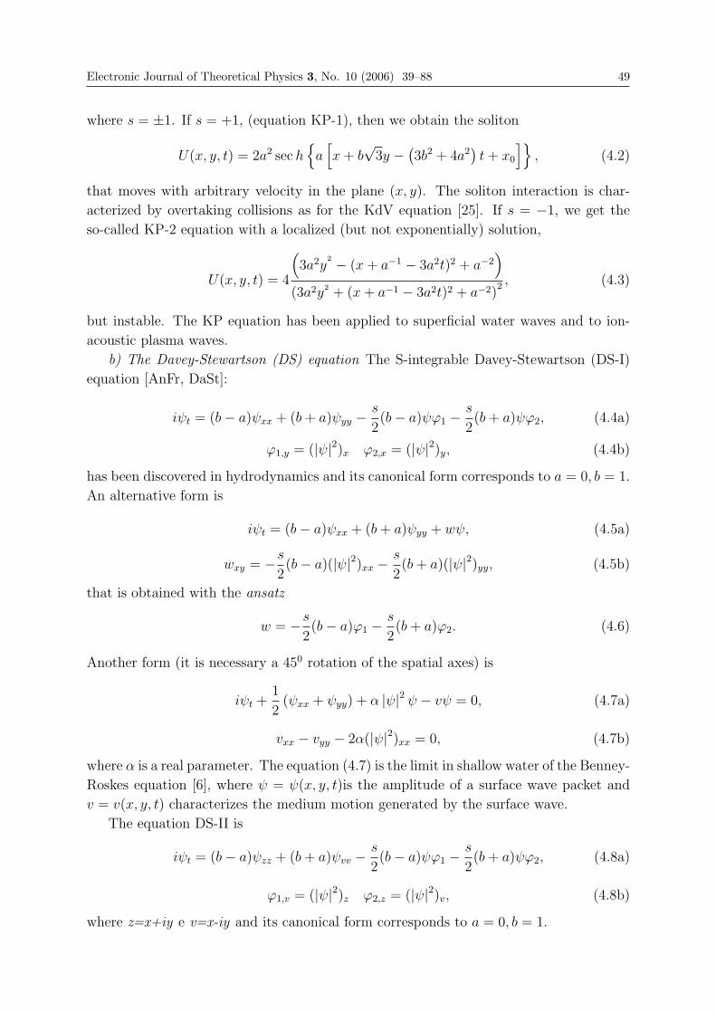
Electronic Journal of Theoretical Physics 3, No. 10 (2006) 39–88 49
where s = ±1. If s = +1, (equation KP-1), then we obtain the soliton
U(x, y, t) = 2a2 sec h{
a[x + b
√3y − (3b2 + 4a2
)t + x0
]}, (4.2)
that moves with arbitrary velocity in the plane (x, y). The soliton interaction is char-
acterized by overtaking collisions as for the KdV equation [25]. If s = −1, we get the
so-called KP-2 equation with a localized (but not exponentially) solution,
U(x, y, t) = 4
(3a2y
2 − (x + a−1 − 3a2t)2 + a−2)
(3a2y2 + (x + a−1 − 3a2t)2 + a−2)2 , (4.3)
but instable. The KP equation has been applied to superficial water waves and to ion-
acoustic plasma waves.
b) The Davey-Stewartson (DS) equation The S-integrable Davey-Stewartson (DS-I)
equation [AnFr, DaSt]:
iψt = (b− a)ψxx + (b + a)ψyy − s
2(b− a)ψϕ1 − s
2(b + a)ψϕ2, (4.4a)
ϕ1,y = (|ψ|2)x ϕ2,x = (|ψ|2)y, (4.4b)
has been discovered in hydrodynamics and its canonical form corresponds to a = 0, b = 1.
An alternative form is
iψt = (b− a)ψxx + (b + a)ψyy + wψ, (4.5a)
wxy = −s
2(b− a)(|ψ|2)xx − s
2(b + a)(|ψ|2)yy, (4.5b)
that is obtained with the ansatz
w = −s
2(b− a)ϕ1 − s
2(b + a)ϕ2. (4.6)
Another form (it is necessary a 450 rotation of the spatial axes) is
iψt +1
2(ψxx + ψyy) + α |ψ|2 ψ − vψ = 0, (4.7a)
vxx − vyy − 2α(|ψ|2)xx = 0, (4.7b)
where α is a real parameter. The equation (4.7) is the limit in shallow water of the Benney-
Roskes equation [6], where ψ = ψ(x, y, t)is the amplitude of a surface wave packet and
v = v(x, y, t) characterizes the medium motion generated by the surface wave.
The equation DS-II is
iψt = (b− a)ψzz + (b + a)ψvv − s
2(b− a)ψϕ1 − s
2(b + a)ψϕ2, (4.8a)
ϕ1,v = (|ψ|2)z ϕ2,z = (|ψ|2)v, (4.8b)
where z=x+iy e v=x-iy and its canonical form corresponds to a = 0, b = 1.
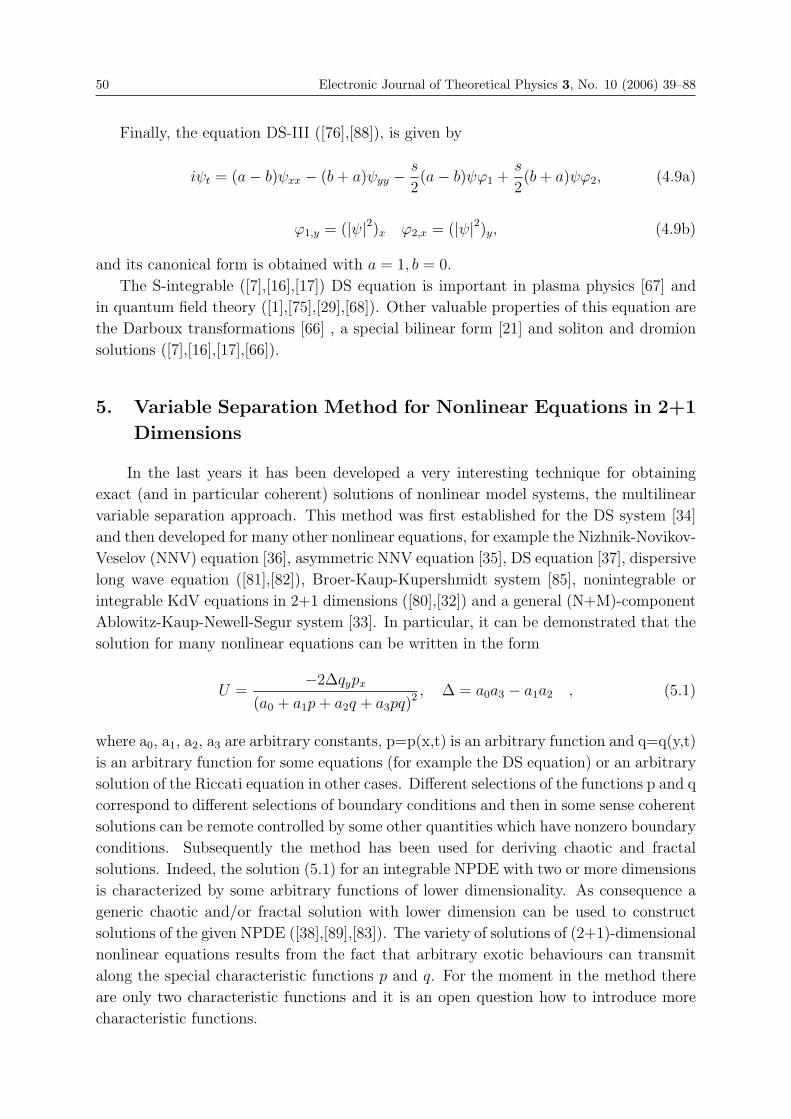
50 Electronic Journal of Theoretical Physics 3, No. 10 (2006) 39–88
Finally, the equation DS-III ([76],[88]), is given by
iψt = (a− b)ψxx − (b + a)ψyy − s
2(a− b)ψϕ1 +
s
2(b + a)ψϕ2, (4.9a)
ϕ1,y = (|ψ|2)x ϕ2,x = (|ψ|2)y, (4.9b)
and its canonical form is obtained with a = 1, b = 0.
The S-integrable ([7],[16],[17]) DS equation is important in plasma physics [67] and
in quantum field theory ([1],[75],[29],[68]). Other valuable properties of this equation are
the Darboux transformations [66] , a special bilinear form [21] and soliton and dromion
solutions ([7],[16],[17],[66]).
5. Variable Separation Method for Nonlinear Equations in 2+1
Dimensions
In the last years it has been developed a very interesting technique for obtaining
exact (and in particular coherent) solutions of nonlinear model systems, the multilinear
variable separation approach. This method was first established for the DS system [34]
and then developed for many other nonlinear equations, for example the Nizhnik-Novikov-
Veselov (NNV) equation [36], asymmetric NNV equation [35], DS equation [37], dispersive
long wave equation ([81],[82]), Broer-Kaup-Kupershmidt system [85], nonintegrable or
integrable KdV equations in 2+1 dimensions ([80],[32]) and a general (N+M)-component
Ablowitz-Kaup-Newell-Segur system [33]. In particular, it can be demonstrated that the
solution for many nonlinear equations can be written in the form
U =−2Δqypx
(a0 + a1p + a2q + a3pq)2 , Δ = a0a3 − a1a2 , (5.1)
where a0, a1, a2, a3 are arbitrary constants, p=p(x,t) is an arbitrary function and q=q(y,t)
is an arbitrary function for some equations (for example the DS equation) or an arbitrary
solution of the Riccati equation in other cases. Different selections of the functions p and q
correspond to different selections of boundary conditions and then in some sense coherent
solutions can be remote controlled by some other quantities which have nonzero boundary
conditions. Subsequently the method has been used for deriving chaotic and fractal
solutions. Indeed, the solution (5.1) for an integrable NPDE with two or more dimensions
is characterized by some arbitrary functions of lower dimensionality. As consequence a
generic chaotic and/or fractal solution with lower dimension can be used to construct
solutions of the given NPDE ([38],[89],[83]). The variety of solutions of (2+1)-dimensional
nonlinear equations results from the fact that arbitrary exotic behaviours can transmit
along the special characteristic functions p and q. For the moment in the method there
are only two characteristic functions and it is an open question how to introduce more
characteristic functions.
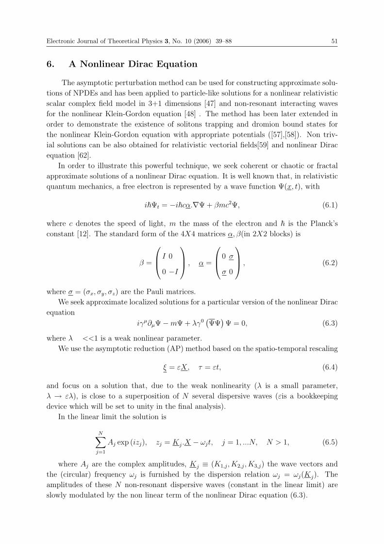
Electronic Journal of Theoretical Physics 3, No. 10 (2006) 39–88 51
6. A Nonlinear Dirac Equation
The asymptotic perturbation method can be used for constructing approximate solu-
tions of NPDEs and has been applied to particle-like solutions for a nonlinear relativistic
scalar complex field model in 3+1 dimensions [47] and non-resonant interacting waves
for the nonlinear Klein-Gordon equation [48] . The method has been later extended in
order to demonstrate the existence of solitons trapping and dromion bound states for
the nonlinear Klein-Gordon equation with appropriate potentials ([57],[58]). Non triv-
ial solutions can be also obtained for relativistic vectorial fields[59] and nonlinear Dirac
equation [62].
In order to illustrate this powerful technique, we seek coherent or chaotic or fractal
approximate solutions of a nonlinear Dirac equation. It is well known that, in relativistic
quantum mechanics, a free electron is represented by a wave function Ψ(x, t), with
i�Ψt = −i�cα.∇Ψ + βmc2Ψ, (6.1)
where c denotes the speed of light, m the mass of the electron and � is the Planck’s
constant [12]. The standard form of the 4X4 matrices α, β(in 2X2 blocks) is
β =
⎛⎜⎝ I 0
0 −I
⎞⎟⎠ , α =
⎛⎜⎝ 0 σ
σ 0
⎞⎟⎠ , (6.2)
where σ = (σx, σy, σz) are the Pauli matrices.
We seek approximate localized solutions for a particular version of the nonlinear Dirac
equation
iγμ∂μΨ−mΨ + λγ0(ΨΨ
)Ψ = 0, (6.3)
where λ <<1 is a weak nonlinear parameter.
We use the asymptotic reduction (AP) method based on the spatio-temporal rescaling
ξ = εX, τ = εt, (6.4)
and focus on a solution that, due to the weak nonlinearity (λ is a small parameter,
λ → ελ), is close to a superposition of N several dispersive waves (εis a bookkeeping
device which will be set to unity in the final analysis).
In the linear limit the solution is
N∑j=1
Aj exp (izj), zj = Kj.X − ωjt, j = 1, ...N, N > 1, (6.5)
where Aj are the complex amplitudes, Kj ≡ (K1,j, K2,j, K3,j) the wave vectors and
the (circular) frequency ωj is furnished by the dispersion relation ωj = ωj(Kj). The
amplitudes of these N non-resonant dispersive waves (constant in the linear limit) are
slowly modulated by the non linear term of the nonlinear Dirac equation (6.3).
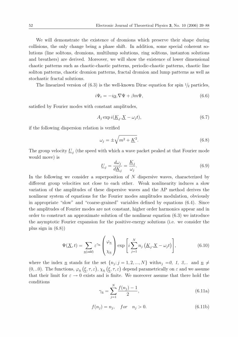
52 Electronic Journal of Theoretical Physics 3, No. 10 (2006) 39–88
We will demonstrate the existence of dromions which preserve their shape during
collisions, the only change being a phase shift. In addition, some special coherent so-
lutions (line solitons, dromions, multilump solutions, ring solitons, instanton solutions
and breathers) are derived. Moreover, we will show the existence of lower dimensional
chaotic patterns such as chaotic-chaotic patterns, periodic-chaotic patterns, chaotic line
soliton patterns, chaotic dromion patterns, fractal dromion and lump patterns as well as
stochastic fractal solutions.
The linearized version of (6.3) is the well-known Dirac equation for spin 1/2 particles,
iΨt = −iα.∇Ψ + βmΨ, (6.6)
satisfied by Fourier modes with constant amplitudes,
Aj exp i(Kj.X − ωjt), (6.7)
if the following dispersion relation is verified
ωj = ±√
m2 + K2. (6.8)
The group velocity U j (the speed with which a wave packet peaked at that Fourier mode
would move) is
U j =dωj
dKj
=Kj
ωj
. (6.9)
In the following we consider a superposition of N dispersive waves, characterized by
different group velocities not close to each other. Weak nonlinearity induces a slow
variation of the amplitudes of these dispersive waves and the AP method derives the
nonlinear system of equations for the Fourier modes amplitudes modulation, obviously
in appropriate “slow” and “coarse-grained” variables defined by equations (6.4). Since
the amplitudes of Fourier modes are not constant, higher order harmonics appear and in
order to construct an approximate solution of the nonlinear equation (6.3) we introduce
the asymptotic Fourier expansion for the positive-energy solutions (i.e. we consider the
plus sign in (6.8))
Ψ(X, t) =∑
n(odd)
εγn
⎛⎜⎝ϕn
χn
⎞⎟⎠ exp
[i
N∑j=1
nj
(Kj.X − ωjt
)], (6.10)
where the index n stands for the set {nj; j = 1, 2, ..., N} withnj =0, 1, 3,.. and n �=(0, ..0). The functions, ϕn
(ξ, τ, ε
), χn
(ξ, τ, ε
)depend parametrically on ε and we assume
that their limit for ε → 0 exists and is finite. We moreover assume that there hold the
conditions
γn =N∑
j=1
f(nj)− 1
2, (6.11a)
f(nj) = nj, for nj > 0. (6.11b)
Electronic Journal of Theoretical Physics 3, No. 10 (2006) 39–88 53
This implies that we obtain the main amplitudes if one of the indices nj has unit modulus
and all the others vanish. In the following we use the notation
ϕj = ϕn(ε→ 0) if nj = 1 and nm = 0 for j �= m, (6.12)
and similar notations for χn.
Taking into account (6.11-6.12), the Fourier expansion (6.10) can be written more
explicitly in the following form
Ψ(X, t) =N∑
j=1
⎡⎢⎣⎛⎜⎝ϕj
χj
⎞⎟⎠ exp(i(Kj.X − ωjt))
⎤⎥⎦+ O(ε). (6.13)
Substituting (6.13) in equation (6.3) and considering the different equations obtained
for every harmonic, we obtain for nj = 1, nm = 0, if j �= m at the lowest order of
approximation
χj = cjϕj =σKj
m + ωj
ϕj, (6.14)
and at the order of approximation of ε:
iϕj,τ = −iσ∇χj + σKχj − λ
N∑m=1
(ϕ+mϕm − χ+
mχm)ϕj, (6.15a)
iχj,τ + ωjχj = −iσ∇ϕj −mχj − λ
N∑m=1
(ϕ+mϕm − χ+
mχm)χj, (6.15b)
where χj is the correction of order ε to χj. After some calculations, we arrive at a system
of equations for the N modulated amplitudes ϕj,
ϕj,τ + U j∇ϕj − iλ
N∑m=1
bm |ϕm|2 ϕj = 0, (6.16)
where U j is the group velocity and bm is a constant coefficient given by
bm =2m
m + ωm
. (6.17)
The system of equations (6.16) is C-integrable by means of an appropriate transformation
of the dependent variables. We set
ϕj(ξ, τ) = ρj(ξ,τ) exp[iϑj(ξ, τ)
], j = 1, ..N, (6.18)
with ρj = ρj(ξ, τ) >0 and ϑj = ϑj(ξ, τ) real functions. Then equation (6.16) yields
ρj,τ + U j∇ρj = 0, (6.19a)
ϑj,τ + U j.∇ϑj − λ
N∑m=1
bmρ2m = 0. (6.19b)
54 Electronic Journal of Theoretical Physics 3, No. 10 (2006) 39–88
The general solution for the Cauchy problem of (6.19a) reads
ρj(ξ, τ) = ρj
(ξ − U jτ
), (6.20)
where the N real functions ρj
(ξ), which represent the initial shape, can be chosen arbi-
trarily. A simple particular case is the solution
ρj = ρj(ajξ + bjτ), (6.21a)
where bj, aj are real constants which satisfy the relation
ajU j + bj = 0. (6.21b)
The general solution of (6.19b) is
ϑj(ξ, τ) = δj(ξ − U jτ) + λ
N∑m=1
bm
∫ τ
0
(ρm(ξ − U j(τ − τ), τ))2dτ , (6.22)
where the N arbitrary functions δj(ξ) are fixed by the initial data. The particular solution
corresponding to (6.21b) is
ϑj(ξ, τ) = δj(ajξ + bjτ) + λ
N∑m=1
bm
∫ τ
0
(ρm(ξ − U j(τ − τ), τ))2dτ , (6.23a)
where
ajU j + bj = 0. (6.23b)
The approximate solution for the system of equations (6.3) is
Ψ(X, t) =N∑
j=1
⎛⎜⎝ 1
cj
⎞⎟⎠ ρj exp[i(ϑj + KjX − ωjt)
]+ O(ε). (6.24)
where cj is given by (6.14). The corrections of order to the approximate solution depend
on higher harmonics and can be easily calculated by the AP method.
a) Solitons. The C-integrable nature of the system (6.19) implies the existence of more
interesting solutions, because of the existence of arbitrary functions in the seed solutions.
It is possible the existence of N solitons, with fixed speeds but arbitrary shapes, which
interact each other preserving their shapes and propagate with the relative group velocity.
The collision of two solitons does not produce a change in the amplitude ρj of each of
them, but only a change in the phase given by equation (6.22).
For instance, we take
ρj(ξ, τ) =2Aj
ch(2Aj(ajξ + bjτ)
) , (6.25)
Electronic Journal of Theoretical Physics 3, No. 10 (2006) 39–88 55
δj = 0 for j=1 .. N, (6.26)
where Aj, for j = 1...N , are real constants, and the phase ϑj is given by (6.22).
Substituting (6.27) in (6.24) we obtain the approximate solution. Each soliton advances
with a constant velocity (the group velocity) before and after collisions. Only the phase
is changed during collisions owing to the presence of the other solitons.
b) Dromions. The existence of localized solutions is possible also for C-integrable sys-
tems, because dromion solutions are not exclusive characteristics of equations integrable
by the inverse scattering method.
A particular solution of the model system (6.19) is given by
ρj(ξ, τ) = Aj exp(−Bj
∣∣ξ − Ujτ∣∣), (6.27)
δj = 0 for j=1, 2. . . .N, (6.28)
where Aj, Bj are real constants (note that the functions ρj (3.4a) are localized) and ϑj
is given by equations (6.22).
c) Lumps. It is well known that in high dimension, in addition to the dromion solu-
tions, other interesting localized solutions, formed by rational functions, are the multiple
lumps. Obviously, there are many possible choices in order to obtain multilump solutions.
For instance, we take
ρj =Aj
Bj + Cj
∣∣ξ − Ujτ∣∣2 , (6.29a)
δj = 0 for j=1, . . . N, (6.29b)
where Aj, Bj and Cj are arbitrary constants.
d) Ring solitons. The multiple ring solitons are solutions that are not equal to zero
at some closed curves and decay exponentially away from the closed curves. A possible
selection is
ρj = Aj exp(−Bjfj(Rj)), (6.30a)
δj = 0 for j=1 .. N. (6.30b)
where
Rj =∣∣ξ − Ujτ
∣∣ , (6.30c)
fj(R) = (R−R0,j)2, (6.30d)
and Aj, Bj and R0,j are arbitrary constants. In Fig. 1 we show a collision between two
ring solitons: the initial condition is showed in Fig. 1a, then the two ring solitons collide
(Fig. 1b) and then separate (Fig. 1c). We can see that these solutions preserve their
shapes but with a phase shift.
56 Electronic Journal of Theoretical Physics 3, No. 10 (2006) 39–88
e) Instantons. If we choose a decaying function of time, we obtain also multiple
instanton solutions, for example,
ρj = Aj exp(ajξ − λjτ), (6.31a)
δj = 0 for j=1 .. N, (6.31b)
where Aj, α1,j are arbitrary constants and
λj = α1,jU1,j + α2,jU2,j. (6.31c)
f) Moving breather-like structures. Finally, if we choose some types of periodic functions
of time in the above mentioned solutions, then we obtain breathers. For example, we
take
ρj = Aj cos(ajξ − Ωjτ) exp[−Bj
∣∣ξ − Ujτ∣∣] , (6.32a)
δj = 0 for j=1 .. N, (6.32b)
where Aj, Bj, α1,jare arbitrary constants and
Ωj = ajU j. (6.32c)
g) Chaotic-chaotic and chaotic-periodic patterns. If we select at least one of the arbitrary
functions in order to contain some chaotic solutions of nonintegrable equations, then
we obtain some type of space-time chaotic patterns, the so-called chaotic-chaotic (in all
spatial directions) patterns. For example, we choose the arbitrary function as solution of
the chaotic Lorenz system
XT = −c(X − Y ), YT = X(a− Z)− Y, ZT = XY − bZ, (6.33a)
witha = 60, b = 8/3, c = 10,or of the Rossler system
XT = −Y − Z, YT = X + aY, ZT = b + Z(X − c), (6.33b)
with a = 0.15, b = 0.2, c = 10and T = ξ−U1τ (or T = ξ−U1τor T = ζ −U3τ). A phase
and amplitude chaotic-chaotic pattern is given by
ρj(ξ, τ) = X(ξ − U1,jτ)Y (η − U2,jτ)Z(ζ − U3,jτ) (6.34a)
δj = 0 for j = 1, . . ..N, (6.34b)
while ϑj is given by equations (6,22). An example is given in Fig. 2.
On the contrary, we obtain a phase chaotic-chaotic pattern, if we choose the function
(6.34b) as solution of the Lorenz system. Finally, if we select a chaotic-periodic solution
which is chaotic in one (or two) direction and periodic in the other(s) direction(s). then
we obtain the so-called chaotic-periodic patterns.
Electronic Journal of Theoretical Physics 3, No. 10 (2006) 39–88 57
h) Chaotic line soliton solutions
If we consider the soliton line solution (6.25-6.26) we can easily deduce a chaotic
solution when we select Aj as solution of the Lorenz system,
ρj(ξ, τ) =2Aj(ξ, τ)
ch(2(ajξ + bjτ)Aj(ξ, τ)
) , (6.35a)
δj = 0 for j=1 .. N, (6.35b)
where the phase ϑj is given as usual by (6.22), for j = 1...N , and the functions Aj =
Aj(Tj) = Aj(ajξ + bjτ) satisfy the third order ordinary differential equation equivalent
to the Lorenz system,
Aj,TTT + (b + c + 1)Aj,TT + (bc + b + A2j)Aj,T + c(b− ab + A2
j)Aj (6.35c)
−Aj,TT Aj,T + (c + 1)A2j,T
Aj
= 0.
i) Chaotic dromion and lump patterns
If we consider the dromion solution (6.27-6.28), we can transform it into a chaotic
pattern with an appropriate choice for Aj and/or Bj,
ρj(ξ, τ) = Aj exp(−Bj
∣∣ξ − Ujτ∣∣), (6.36a)
δj = 0 for j=1, 2. . . .N, (6.36b)
where Aj = Aj(Tj) = Aj(ajξ + bjτ) and/or Bj = Bj(Tj) = Bj(ajξ + bjτ) are solutions
of the Lorenz equation and ϑj is given by equations (6.22). We obtain an amplitude (Aj
chaotic) or a shape (Bj chaotic) or an amplitude and shape (Aj and Bj chaotic) dromion
chaotic pattern. Similar considerations can be applied to the lump solutions (6.29).
j) Nonlocal fractal solutions. If we choose
ρj(ξ, τ) =3∏
m=1
Tm,j |Tm,j|{sin
[ln(T 2
m,j
)]− cos[ln(T 2
m,j
)]}(6.37)
with T = (T1, T2, T3), T j = ξ−U jτ , we get a nonlocal fractal structure for small T j. It is
well known that if we plot the structure of the solution at smaller regions we can obtain
the same structures.
k) Fractal dromion and lump solutions. A fractal dromion (lump) solution is expo-
nentially (algebraically) localized in large scale and possesses self-similar structure near
the center of the dromion. We consider for example an amplitude fractal dromion
ρj(ξ, τ) = Aj exp(−Bj
∣∣ξ − Ujτ∣∣), (6.38a)
58 Electronic Journal of Theoretical Physics 3, No. 10 (2006) 39–88
δj = 0 for j=1, 2. . . .N, (6.38b)
where ϑj is given by equations (6.22) and Aj = Aj(Tj) = Aj(ajξ + bjτ) is given by
Aj = 2 + sin{ln[T 2
j
]}. (6.38c)
By a similar choice for Bj or δjwe obtain shape or phase fractal dromion.
l) Stochastic fractal dromion and lump excitations. It is well known the stochastic
fractal property of the continuous but nowhere differentiable Weierstrass function
W (x) =N∑
k=1
(c1)k sin
[(c2)
k x], N →∞, (6.39a)
with c2 odd and
c1c2 > 1 +3π
2. (6.39b)
A stochastic fractal solution is (see Fig. 3 for an example)
ρj(ξ, τ) =3∏
m=1
Am,j(ξm − Um,jτ), (6.40a)
δj = 0 for j=1, 2. . . .N, (6.40b)
where ϑj is as usual given by equations (6.22), Aj = (A1,j, A2,j, A3,j), ξ1 = ξ,ξ2 =
η,ξ3 = ζ, and Aj = Aj(ξ − U jτ) is given by
Aj = W (ξ − U jτ) + (ξ − U jτ)2. (6.40c)
m) Stochastic fractal dromion and lump excitations. In order to obtain a stochastic
amplitude fractal dromion we choose
ρj(ξ, τ) = Aj exp(−Bj
∣∣ξ − Ujτ∣∣), (6.41a)
δj = 0 for j=1, 2. . . .N, (6.41b)
where ϑj is given by equations (6.22) Aj = Aj(Tj) = Aj(ajξ + bjτ) is given by
Aj = W (Tj) + T 2j (6.41c)
By similar methods we obtain shape or phase stochastic fractal dromion as well as stochas-
tic fractal lump solutions.
Electronic Journal of Theoretical Physics 3, No. 10 (2006) 39–88 59
7. Spontaneous Symmetry Breaking Model
We now illustrate in some detail the use of the AP method and consider a scalar
complex field Φ = Φ(x), x = (x0 = t, x), coupled with a massless vectorial gauge field
Aμ = Aμ(x), Aμ = (A0, A), and seek approximate localized solutions for a spontaneous
symmetry breaking (or hidden symmetry or Higgs) model ([19],[22],[23]) with Lagrangian
[63]
L = [(∂μ + iqAμ) Φ]∗ [(∂μ + iqAμ) Φ]− 1
4FμνF
μν − a2
2b2(Φ∗Φ)2 +
a2
2(Φ∗Φ), (7.1a)
Fμν = ∂μAν − ∂νAμ. (7.1b)
The Lagrangian (7.1) is invariant under the local transformation
Φ(x)→ Φ′(x) = exp (−iα(x)Φ(x)) , (7.2a)
with accompanied by the gauge transformation on the potentials
Aμ(x)→ A′μ(x) = Aμ(x) +1
q∂μα(x). (7.2b)
We note that this model contains four field degrees of freedom, two in the complex scalar
Higgs field and two in the massless gauge field. The field equations are
∂μ∂μAν − ∂ν(∂μA
μ) = Jν , (7.3a)
Jν = iq [Φ∗ (∂νΦ)− (∂νΦ∗) Φ]− 2q2Aν |Φ|2 , (7.3b)
∂μ∂μΦ− a2
2Φ = −a2
b2|Φ|2 Φ, (7.3c)
where ∂μ∂μ = ∂2
t −∇2, a, b and q are parameters. The potential for the scalar field is
V (Φ) = −a2
2|Φ|2 +
a2
2b2|Φ|4 , (7.4)
and the physical vacuum is identified by the condition
|Φ|2 = b2. (7.5)
We consider the interaction and eventually the collisions among coherent solutions with
different velocities that are not close to each other and use the asymptotic reduction (AP)
method based on the spatio-temporal rescaling
ξ = ε2x, (7.6)
where
ξ = (ξ0, ξ), x = (x0, x). (7.7)
and the small positive nondimensional parameter ε is artificially introduced to serve as
bookkeeping device and will be set equal to unity in the final analysis. The linear evo-
lution is most appropriately described in terms of Fourier modes, which have a constant
60 Electronic Journal of Theoretical Physics 3, No. 10 (2006) 39–88
amplitude and a well defined group velocity (the speed with which a wave packet peaked
at that Fourier mode would move in ordinary space). We study the modulation, in terms
of the variables defined above, of the amplitude of the Fourier mode. The modulation
(that would remain constant in the absence of nonlinear effects) is best described in terms
of the rescaled variables, ξ, that account for the need to look on larger space and time
scales, to obtain a not negligible contribution from the nonlinear term. The reduction
method focuses on a solution that is small and is close to a superposition of N several
dispersive waves, with different group velocities.
In the linear limit the solution is a linear combination of dispersive waves. For example
for the scalar field the linear solution is
N∑j=1
Cj exp (−isj), sj = kj,μxμ = ωjt− Kj.x, (7.8)
where Cj are the complex amplitudes, kμj = (ωj, Kj), Kj ≡ (K1,j, K2,j, K3,j) the wave
vectors and the (circular) frequency ωj is furnished by the dispersion relation ωj = ωj(Kj).
The amplitudes of these N non-resonant dispersive waves (constant in the linear limit)
are slowly modulated by the nonlinear terms. We derive a model system of equations
for the slow modulation of the Fourier modes amplitudes and, subsequently, show that
it is C-integrable. The Cauchy problem is resolved, just by quadratures, and explicit
nontrivial solutions are constructed.
We introduce two real Higgs fields U = U(x, t) e W = W (x, t) and set
Φ =1√2
(b + U + iW ) . (7.9)
In the following we use the covariant ‘t Hooft gauge [tHo], which for this Abelian model
is (M=qb)
∂μAμ = λMW, (7.10)
where λ is an arbitrary parameter. For any finite λ, we obtain R gauges, that are
manifestly renormalisable, but involve unphysical Higgs fields such as W . We recall that
in the limit λ→∞ we obtain the U (unitary) gauge, where only physical particles appear.
Using (7.1-7.8), the equations (7.9-7.11) yield
(∂μ∂
μ + M2)Aν −
(1− 1
λ
)∂ν(∂μA
μ) = Jν , (7.11)
Jν = q
[(∂νU − U∂ν) (∂μA
μ)
λM
]− q2Aν
[U2 + 2bU +
(∂μAμ)2
λ2M2
], (7.12)
(∂μ∂
μ + M2)U = −a2U2
2b− a2
2b
(1 +
U
b
)(U2 +
(∂μAμ)2
λ2M2
). (7.13)
We consider now a superposition of N dispersive waves, characterized by different values
of the wave vector Kj and by group velocities not close to each other. Weak nonlinearity
Electronic Journal of Theoretical Physics 3, No. 10 (2006) 39–88 61
induces a slow variation of the amplitudes of these dispersive waves and the AP method
derives the nonlinear system of equations for the Fourier modes amplitudes modulation,
obviously in appropriate “slow” and “coarse-grained” variables defined by equations (7.7).
Since the amplitude of Fourier modes are not constant, higher order harmonics appear
and in order to construct an approximate solution that is small of order ε and that is close
in the limit of small ε to the linear solution (7.8), we introduce the asymptotic Fourier
expansion
U(xμ) =∞∑
n=−∞exp
(i
N∑j=1
nj sj
)εγnϕn(ξμ; ε), sj = kj,μx
μ = ωjt− Kj.x, (7.14)
Aν(xμ) =∞∑
n=−∞exp
(i
N∑j=1
njsj
)εγnψn(ξμ; ε), sj = kj,μx
μ = ωjt−Kj.x, (7.15)
where the index n stands for the set {nj; j = 1, 2, ..., N}. In the expansion (7.14) nj =
0,±1,±2, .., while in the expansion (7.15) nj may assume only odd values, nj = ±1,±3...
The functions, ψνn(ξ; ε), ϕn(ξ; ε) depend parametrically on ε and we assume that their
limit for ε→ 0 exists and is finite. We moreover assume that there hold the conditions
γn = γ−n, γn =N∑
j=1
|nj|. (7.16)
This implies that we obtain the main amplitudes if one of the indices nj has unit modulus
and all the others vanish. We use the following notations, for j = 1, 2, ...N ,
ϕn(ξ, ε→ 0) = ϕj(ξ), if nj = 1 and nm = 0 for j �= m, (7.17a)
ϕn(ξ; ε→ 0) = ϕ0(ξ), if nj = 0, (7.17b)
ϕn(ξ; ε→ 0) = ϕ2,j(ξ), if nj = 2 and nm = 0 for j �= m, (7.17c)
ϕn(ξ; ε→ 0) = ϕ11,jm(ξ), if nj = nm = 1 and nl = 0 for l �= j, m, j �= m,
(7.17d)
ϕn(ξ; ε→ 0) = ϕ1−1,jm(ξ), if nj = 1, nm = −1, and nl = 0 for l �= j, m , j �= m,
(7.17e)
while for the vectorial field we set
Ψνn(ξ; ε→ 0) = Ψν
j (ξ). (7.18)
62 Electronic Journal of Theoretical Physics 3, No. 10 (2006) 39–88
Taking into account (7.17-7.18), the Fourier expansion (7.14-7.15) can be written more
explicitly in the following form
Aν(x) = ε
N∑j=1
[exp(isj)Ψ
νj (ξ) + c.c.
]+ O(ε3), (7.19)
U(x) = εN∑
j=1
[exp(isj)ϕj(ξ) + ε exp(2isj)ϕ2,j(ξ) + c.c.] + ε2ϕ0(ξ)
+ε2N∑
j,m=1,j �=m
[exp(−isj − ism)ϕ11,jm(ξ) + exp(−isj + ism)ϕ1−1,jm(ξ) + c.c.] + O(ε3)
(7.20)
where c.c. stands for complex conjugate.
The standard procedure is to consider the different equations obtained from the co-
efficients of the Fourier modes. Substituting (7.19-7.20) in equations (7.11-7.15) and
considering the different equations obtained for every harmonic and for a fixed order of
approximation in ε, we obtain for nj = 1, nm = 0, if j �= m, to the order of ε, the
following system of equations for the main modulated amplitudes,
(−kj,μkμj + a2)ϕj = 0, (7.21a)
[(−kj,σk
σj + M2)gνμ +
(1− 1
ξ
)(kμ
j kνj )
]Ψj,μ = 0. (7.21b)
From (7.21a-b) we obtain the dispersion relations
ω2j = K
2
j + a2, ω2j = K2
j + M2, (7.22a)
with the associated group velocities
Vj =Kj
ωj
, Vj =Kj
ωj
. (7.22b)
Moreover, from (7.21b), as a consequence of the gauge invariance of the vectorial field
(only three components of the fields are independent), we obtain
kμj Ψj,μ = ωjΨj,0 −KΨ = 0. (7.23)
We obtain for nj = 1, nm = 0, if j �= m, to the order of ε2,
(−2ikj,μ∂μ)ϕj +
3a2
2b
(2ϕ0ϕj + 2ϕ2ϕ
∗j + |ϕj|2 ϕj
)(7.24a)
+3a2
b2
N∑m=1,m�=j
(|ϕm|2 ϕj + ϕ11,jmϕ∗j + ϕ1−1,jmϕj
)= 0
,
Electronic Journal of Theoretical Physics 3, No. 10 (2006) 39–88 63
[(−2kj,σ∂
σ)gνμ +
(1− 1
λ
)(∂μkν
j )
]Ψj,μ + i
(−2q2Ψνj
)( N∑m=1
|ϕm|2 + bϕ0
)= 0, (7.24b)
and for nj = 0, to the order of ε2,
ϕ0 = A
N∑m=1
|ϕm|2, A = −3
b, (7.25)
and for nj = 2, nm = 0, if j �= m, to the order of ε2,
ϕ2,j = B2ϕ2j , B2 = − 1
2b(7.26)
and for nj = 1, nm = 1, nl = 0 if j, m �= l, to the order of ε2,
ϕ11,jm =N∑
m=1
B11,jmϕjϕm, B11,jm =3a2
b(a2 + 2kμ
mkj,μ
) , (7.27)
and for nj = 1, nm = −1, nl = 0, if j, m �= l, to the order of ε2,
ϕ1−1,jm =N∑
m=1
B1−1,jmϕjϕ∗m, B1−1,jm =
3a2
b(a2 − 2kμ
mkj,μ
) . (7.28)
Using (7.24a-b) then equations (7.21-7.22) yield
(kj,μ∂μ)ϕj + i
N∑m=1
[αjm |ϕm|2
]ϕj = 0, (7.29a)
[(−2kj,σ∂
σ)gνμ +
(1− 1
λ
)(∂μkν
j )
]Ψj,μ + iβ
N∑m=1
[|ϕm|2]Ψν
j = 0, (7.29b)
where the coefficients α, β, are depending on the wave vectors of the scalar and vectorial
fields,
αjm = −3a2
b2+
9a6
b2(a4 − 4 (kμ
mkj,μ)2) , j �= m, (7.30a)
αjj = −9a2
2b2, β = 4q2. (7.30b)
The system of equations (7.28-7.29) is C-integrable by means of an appropriate transfor-
mation of the dependent variables. We set
ϕj(ξ) = ρj(ξ) exp [iϑj(ξ)] , j = 1, ..N, (7.31a)
Ψνj (ξ) = χν
j (ξ) exp[iδν
j (ξ)], j = 1, ..N, (7.31b)
64 Electronic Journal of Theoretical Physics 3, No. 10 (2006) 39–88
with ρj = ρj(ξ), χνj = χν
j (ξ) >0 and ϑj = ϑj(ξ), δνj = δν
j (ξ) real functions. Then equation
(7.28-7.29) yield
(kj,μ∂μ)ρj = 0, (7.32a)
(kj,μ∂μ)ϑj +
N∑m=1
[αjmρ2
m
]= 0, (7.32b)
and [(−2kj,σ∂
σ)gνμ + (1− 1
λ)(kν
j ∂μ)
]χj,μ = T μν
j χj,μ = 0, (7.33a)
[(−2kj,σ∂
σ)χνj g
νμ +
(1− 1
λ
)χν
j (∂μkν
j )
]δj,μ + β
N∑m=1
[|ϕm|2 χνj
]= 0 (7.33b)
We now consider a particular mode j with group velocity V j = 0, i. e. Kj = 0 (see
(7.22b)). This condition is equivalent to choose a frame where the solution of (7.33a) is
not depending on the time (the proper frame). Equations (7.33a-b) yield
χij = gi
j(ξ), δij = δi
j(ξ) + βτ
N∑m=1
gij(ξ), for i = 1, 2, 3 (7.34)
where gij(ξ), δi
j(ξ) are arbitrary functions of the space variables. Note that g0j (ξ) and
δ0j (ξ) are fixed by the gauge condition (7.31). By a Lorentz boost we can construct the
solution in a generic frame and in the following we use a frame moving con velocity
V j = (Vj, 0, 0)with respect to the proper frame
ξ = γj(ξ′−Vjτ
′), η = η′, ς = ς ′, τ = γj(τ′−Vjξ
′
c2), γj =
(1−
(Vj
c
)2)− 1
2
. (7.35)
On a similar way we obtain the solution for the Higgs field,
ρj = fj(ξ), ϑj = ϑj(ξ)− τ
N∑m=1
αjmf 2m(ξ) (7.36)
where fj(ξ), ϑj(ξ) are arbitrary functions of the space variables.
At last, an interesting particular solution for the Cauchy problem of (7.32a-7.33a)
reads
ρj(ξ, τ) = ρj
(V σ
j ξσ
), (7.37a)
χνj (ξ, τ) = χν
j
(V σ
j ξσ
), (7.37b)
where the 4N real functions ρj
(ξ), χi
j
(ξ), i=1, 2, 3, which represent the initial shape,
can be chosen arbitrarily and
kj,μVμj = 0, kj,μV
μj = 0. (7.38)
Electronic Journal of Theoretical Physics 3, No. 10 (2006) 39–88 65
Inserting (7.37b) in (7.33a) yields[(−2kj,σV
σj )gνμ + (1− 1
λ)(kν
j Vμj )
]χj,μ = T μν
j χj,μ = 0, (7.39)
and since
det T = 8
(2−
(1− 1
λ
))(kj,μV
μj )4 = 0, (7.40)
we obtain
χj,μVμj = 0. (7.41)
The field χ0j(ξ) is fixed by the gauge condition (7.41).
In conclusion, the approximate solution for the system of equations (7.11-7.13) is
Aν(x) = 2εN∑
j=1
χνj exp
[i(δν
j − kj,μxμ)]+ O(ε3), (7.42)
U(x) = εU1(x) + ε2U2(x) + O(ε3), (7.43a)
where
U1(x) = 2εN∑
j=1
[ρj cos(kj,μx
μ − ϑj)], (7.43b)
U2(x) = 2ε2
N∑j=1
[B2ρ
2j cos
[2(kj,μx
μ − ϑj
)]]+ ε2
(Aρ2
j
)(7.43c)
+ε2
N∑j,m=1,j �=m
[B11,jmρjρm cos
[(kj,μx
μ − ϑj
)+(km,μx
μ − ϑm
)]]+ε2
N∑j,m=1,j �=m
[B1−1,jmρjρm cos
[(kj,μx
μ − ϑj
)−(km,μx
μ − ϑm
)]].
The corrections of order to the approximate solution depend on higher harmonics and
can be easily calculated by the AP method.
The validity of the approximate solution should be expected to be restricted on
bounded intervals of the τ -variable and on time-scale t = O( 1ε2 ). If one wishes to study
solutions on intervals such that τ = O(1ε) then the higher terms will in general affect the
solution and must be included.
8. Coherent Solutions
In the following we have written the solutions in the moving frame of reference, but
for simplicity we have dropped the apices in the space and time variables.
66 Electronic Journal of Theoretical Physics 3, No. 10 (2006) 39–88
i) Nonlinear wave. The most simple solution of the system (7.29) is the plane wave
ρj = Aj = constant, ϑj = K′
jξ − ω′jτ (8.1a)
χμj = Bμ
j = constant, δμj = K
′jξ − ω
′′jτ (8.1b)
where the amplitudes and wave vectors are connected according to the nonlinear
dispersion relation
ω′j = V j.K
′j +
α
ω′j
N∑m=1
A2m, ω
′j = V j.K
′
j +1
ωj
N∑m=1
αjmA2m, (8.1c)
χ0j and δ0
j are fixed by the gauge condition (7.23).
ii) Solitons. In the following we seek coherent solutions and use the gauge condition
(7.23) which implies, being χνj = (χ0
j , χj),
χ0j =
Kj.χj
ωj
. (8.2)
The C-integrable nature of the system (7.29) implies the existence of more interesting
solutions, because of the existence of arbitrary functions in the seed solutions. It is
possible the existence of N solitons, with fixed speeds but arbitrary shapes, which interact
each other preserving their shapes and propagate with the relative group velocity. The
collision of two solitons does not produce a change in the amplitude ρj of each of them,
but only a change in the phase given by equation (7.36).
For instance, we take
ρj(ξ, τ) =2Aj
ch(2Aj γj(ξ − Vjτ)
) , (8.3a)
χij(ξ, τ) =
2Aj
ch (2Ajγj(ξ − Vjτ)), for i=1, 2, 3, (8.3b)
ϑj = δνj = 0 for j=1 .. N, (8.3c)
where Aj, for j = 1...N , are real constants,
γj =
⎛⎝1−(
Vj
c
)2⎞⎠− 1
2
, (8.3d)
γj is given by (7.35b) and the phase ϑj and δνj are given by (7.34-7.36). Each soliton
advances with a constant velocity (the group velocity) before and after collisions. Only the
phase is changed during collisions owing to the presence of the other solitons. Substituting
(8.3) in (7.42-7.43) we obtain the approximate solution good to the order of ε. Each
Electronic Journal of Theoretical Physics 3, No. 10 (2006) 39–88 67
soliton advances with a constant velocity (the group velocity) before and after collisions.
Only the phase is changed during collisions owing to the presence of the other solitons.
iii) Dromions. The existence of localized solutions is possible also for C-integrable sys-
tems, because dromion solutions are not exclusive characteristics of equations integrable
by the inverse scattering method.
A particular solution of the model system is given by
ρj(ξ, τ) = Aj exp
(−Bj
√γ2
j (ξ − Vjτ)2 + η2 + ς2
), (8.4a)
χij(ξ, t) = Ai
j exp(−Bi
j
√γ2
j (ξ − Vjτ)2 + y2 + z2))
, for i=1, 2, 3 (8.4b)
ϑj = δνj = 0 for j=1, 2. . . .N, (8.4c)
where Aj, Aj,Bj, Bj are real constants and ϑj and δνj are given by equations (7.34-7.36).
Substituting the solution (8.4) in equation (7.42-7.43) and taking N = 2 we obtain for
two dromions with different shapes and amplitudes the approximate solution
U(x, t) = 22∑
j=1
Aj exp
(−Bj
√γ2
j (x− Vjt)2 + y2 + z2)
)cos(kμ,jx
μ + ϑj), (8.5)
Aν(x, t) = 22∑
j=1
Aνj exp
(−Bν
j
√γ2
j (x− Vjt)2 + y2 + z2))
cos(kμ,jxμ + δj). (8.6)
In Fig. 4 we show a collision between two dromions for the Higgs field (see (7.43b) and
(8.5) with identical mass M = 100 GeV/c2, B1 = B2 = M , P1 = 1600 TeV/c, P2=2000
TeV/c): the initial condition is showed in Fig. 4a, then the two dromions collide (Fig.
4b) and then separate (Fig. 4c). We can see that dromions preserve their shapes but
with a phase shift.
iv) Lumps. It is well known that in high dimension, in addition to the dromion solu-
tions, other interesting localized solutions, formed by rational functions, are the multiple
lumps. Obviously, there are many possible choices in order to obtain multilump solutions.
For instance, we take
ρj(ξ, τ) =Aj
Bj + Cj
√γ2
j
(ξ − Vjτ
)2
+ η2 + ς2
, (8.7a)
χij(ξ, τ) =
Aij
Bij + Ci
j
√γ2
j (ξ − Vjτ)2 + η2 + ς2
, fori=1, 2, 3, (8.7b)
ϑj = δνj = 0 for j=1, . . . N, (8.7c)
where Aj, Bj, Cj, Aij, Bi
j and Cij are arbitrary constants and ϑν
j and δνj are given by
equations (7.34-7.36).
68 Electronic Journal of Theoretical Physics 3, No. 10 (2006) 39–88
v) Ring solitons. The multiple ring solitons are solutions that are not equal to zero
at some closed curves and decay exponentially away from the closed curves. A possible
selection is
ρj(ξ, τ) = Aj exp(−Bjfj(Rj(ξ, τ))), (8.8a)
χij(ξ, τ) = Ai
j exp(−Bijfj(Rj(ξ, τ))), for i=1, 2, 3, (8.8b)
ϑj = δνj = 0 for j=1 .. N. (8.8c)
where
Rj =
√γ2
j
(ξ − Vjτ
)2
+ η2 + ς2, Rj =√
γ2j (ξ − Vjτ)2 + η2 + ς2, (8.9a)
fj(Rj) = (Rj −R0,j)2, fj(Rj) = (Rj − R0,j)
2, (8.9b)
and Aj, Aij, Bj, Bi
j, R0,jand R0,j are arbitrary constants. In Fig. 5 we show a collision
between two ring solitons for the Higgs field (see (7.43b) and (8.8a) with identical mass
M = 100 GeV/c2, B1 = B2 = M2, P1 = P2=2000 TeV/c, R1 = 6/M, R2 = 12/M): the
initial condition is showed in Fig. 5a, then the two ring solitons collide (Fig. 5b) and
then separate (Fig. 5c). We can see that these solutions preserve their shapes but with
a phase shift.
vi) Instantons. If we choose a decaying function of time, we obtain also multiple
instanton solutions, for example,
ρj(ξ, τ) = Aj exp[−Bj γj
(ξ − Vjτ
)], (8.10a)
χij(ξ, τ) = Ai
j exp[−Bi
jγj (ξ − Vjτ)], for i=1, 2, 3, (8.10b)
ϑj = δνj = 0 for j=1 .. N, (8.10c)
where Aj, Aij, Bj, Bi
j are arbitrary constants.
vii) Moving breather-like structures. Finally, if we choose some types of periodic func-
tions of time in the above mentioned solutions, then we obtain breathers. For example,
we take
ρj(ξ, τ) = Aj cos(γj
(ξ − Vjτ
)) exp
[−Bj
√γ2
j
(ξ − Vjτ
)2
+ η2 + ς2
], (8.11a)
χij(ξ, τ) = Ai
j cos(γj (ξ − Vjτ)) exp
[−Bi
j
√γ2
j (ξ − Vjτ)2 + η2 + ς2
], for i=1, 2, 3,
(8.11b)
ϑj = δνj = 0 for j=1 .. N, (8.11c)
where Aj, Aij, Bj, Bi
jare arbitrary constants.
Electronic Journal of Theoretical Physics 3, No. 10 (2006) 39–88 69
9. Chaotic and Fractal Solutions
i) Chaotic-chaotic and chaotic-periodic patterns. If we select at least one of the
arbitrary functions of Section 7 in order to contain some chaotic solutions of nonintegrable
equations, then we obtain some type of space-time chaotic patterns, the so-called chaotic-
chaotic (in all spatial directions) patterns. For example, we choose the arbitrary function
as solution of the chaotic Lorenz system
XT = −c(X − Y ), YT = X(a− Z)− Y, ZT = XY − bZ, (9.1a)
witha = 60, b = 8/3, c = 10,or of the Rossler system
XT = −Y − Z, YT = X + aY, ZT = b + Z(X − c), (9.1b)
with a = 0.15, b = 0.2, c = 10and T = γ(ξ − V τ) (or T = η or T = ς). A phase and
amplitude chaotic-chaotic pattern is given by
ρj(ξ, τ) = X(γj(ξ − Vjτ))Y (η)Z(ζ), (9.2a)
χij(ξ, τ) = X i
j(γj(ξ − Vjτ))Y ij (η)Zi
j(ζ), for i=1, 2, 3, χ0j =
Kj.χj
ωj
(9.2b)
ϑj = δνj = 0 for j=1, 2. . . .N, (9.2c)
while ϑj and δνj is given by equations (7.34-7.36). An example is given in Fig. 6, for the
Higgs field ((7.43b) and (9.2a)) with M = 100 GeV/c2 and γ = 50.
On the contrary, we obtain a phase chaotic-chaotic pattern, if we choose the function
(9.2c) as solution of the Lorenz system. Finally, if we select a chaotic-periodic solution
which is chaotic in one (or two) direction and periodic in the other(s) direction(s). then
we obtain the so-called chaotic-periodic patterns.
ii) Chaotic line soliton solutions
If we consider the soliton line solution (8.3), we can easily deduce a chaotic solution
when we select Aj as solution of the Lorenz system,
ρj(ξ, τ) =2Aj(ξ, τ)
ch(2γj(ξ − Vjτ)Aj(ξ, τ)
) , ϑj = δνj = 0 for j=1 .. N, (9.3a)
χij(ξ, τ) =
2Aij(ξ, τ)
ch(2γj(ξ − Vjτ)Ai
j(ξ, τ)) , for i=1, 2, 3, χ0
j =Kj.χj
ωj
(9.3b)
where the phases ϑj and δνj are given as usual by (7.34-7.36), for j = 1...N , and the
functions Aij = Ai
j(Tj) = Aij(γj(ξ − Vjτ)) satisfy the third order ordinary differential
equation equivalent to the Lorenz system (9.1),
Aj,TTT + (b + c + 1)Aj,TT + (bc + b + A2j)Aj,T + c(b− ab + A2
j)Aj
−Aj,TT Aj,T +(c+1)A2j,T
Aj= 0.
(9.4)
70 Electronic Journal of Theoretical Physics 3, No. 10 (2006) 39–88
iii) Chaotic dromion and lump patterns
If we consider the dromion solution (8.4), we can transform it into a chaotic pattern
with an appropriate choice for Aj and/or Bj,
ρj(ξ, τ) = Aj exp(−Bj
√γ2
j
(ξ − Vjτ
)2
+ η2 + ς2), (9.5a)
χij(ξ, τ) = Ai
j exp
(−Bi
j
√γ2
j (ξ − Vjτ)2 + η2 + ς2
), for i=1, 2, 3, χ0
j =Kj.χj
ωj
(9.5b)
ϑj = δνj = 0 for j=1, 2. . . .N, (9.5c)
where the function Aj = Aj(Tj) = Aj(γj(ξ − Vjτ)) and/or the other amplitude and
shape functions Bj = Bj(Tj) = Bj(γj(ξ − Vjτ)),for the scalar field, and Aij = Ai
j(Tj) =
Aij(γj(ξ − Vjτ)) andBi
j = Bij(Tj) = Bi
j(γj(ξ − Vjτ)) for the vectorial field are solutions
of the Lorenz equation (9.4) and ϑjand δνj are given by equations (7.34-7.36). We obtain
an amplitude (Aj chaotic) or a shape (Bj chaotic) or an amplitude and shape (Aj and
Bj chaotic) dromion chaotic pattern. Similar considerations can be applied to the lump
solutions (8.7).
iv) Nonlocal fractal solutions. If we choose
ρj(ξ, τ) =3∏
m=1
Tm,j
∣∣∣Tm,j
∣∣∣ {sin[ln(T 2
m,j
)]− cos
[ln(T 2
m,j
)]}(9.6a)
χij(ξ, τ) =
3∏m=1
Tm,j |Tm,j|{sin
[ln(T 2
m,j
)]− cos[ln(T 2
m,j
)]}, for i=1, 2, 3, χ0
j =Kj.χj
ωj
(9.6b)
with T j = (T1,j, T2,j, T3,j), T j = (γj(ξ − Vjτ), η, ς), T j = (T1,j, T2,j, T3,j), T j = (γj(ξ −Vjτ), η, ς)we get a nonlocal fractal structure for small T jand T j. It is well known that if
we plot the structure of the solution at smaller regions we can obtain the same structures.
v) Fractal dromion and lump solutions. A fractal dromion (lump) solution is expo-
nentially (algebraically) localized in large scale and possesses self-similar structure near
the center of the dromion. We consider for example an amplitude fractal dromion
ρj(ξ, τ) = Aj exp(−Bj
√γ2
j
(ξ − Vjτ
)2
+ η2 + ς2), (9.7a)
χij(ξ, τ) = Aj exp(−Bj
√γ2
j (ξ − Vjτ)2 + η2 + ς2), for i=1, 2, 3, χ0j =
Kj.χj
ωj
(9.7b)
ϑj = δνj = 0 for j=1, 2. . . .N, (9.7c)
where ϑj and δνj are given by equations (7.34-7.36) and Ai
j = Aij(Tj) = Ai
j(γj(ξ − Vjτ)),
Aj = Aj(Tj) = Aj(γj(ξ − Vjτ)) are given by
Aij(Tj) = Aj(Tj) = 2 + sin
{ln[T 2
j
]}. (9.8)
Electronic Journal of Theoretical Physics 3, No. 10 (2006) 39–88 71
By a similar choice for Bj or Bj, δj, ϑjwe obtain shape or phase fractal dromion.
vi) Stochastic fractal dromion and lump excitations. It is well known the stochastic
fractal property of the continuous but nowhere differentiable Weierstrass function
W (x) =N∑
k=1
(c1)k sin
[(c2)
k x], N →∞, (9.9a)
with c2 odd and
c1c2 > 1 +3π
2. (9.9b)
A stochastic fractal solution is
ρj(ξ, τ) = A1,j(γj(ξ − Vjτ))A2,j(η)A3,j(ς), (9.10a)
χij(ξ, τ) = Ai
1,j(γj(ξ − Vjτ))Ai2,j(η)Ai
3.j(ς), for i=1, 2, 3, χ0j =
Kj.χj
ωj
(9.10b)
ϑj = δνj = 0 for j=1, 2. . . .N, (9.10c)
where ϑj and δνj are as usual given by equations (7.34-7.36), Aj = (A1,j, A2,j, A3,j),
Aj = (A1,j, A2,j, A3,j), and Aj = Aj(γj(ξ−Vjτ), η, ς), Aj = Aj(γj(ξ− Vjτ), η, ς) are given
by
A1,j(γj(ξ − Vjτ)) = A1,j(γj(ξ − Vjτ)) = W (γj(ξ − Vjτ)) + γ2j (ξ − Vjτ)2, (9.11a)
A2,j(η) = A2,j(η) = W (η) + (η)2 , A3,j(ς) = A3,j(ς) = W (ς) + (ς)2. (9.11b)
An example is given in Fig. 4 for the Higgs field (7.43b) and (9.10a) with M = 100
GeV/c2 and γ = 50.
vii) Stochastic fractal dromion and lump excitations. In order to obtain a stochastic
amplitude fractal dromion we choose
ρj(ξ, τ) = Aj exp(−Bj
√γ2
j
(ξ − Vjτ
)2
+ η2 + ς2), (9.12a)
χij(ξ, τ) = Ai
j exp(−Bij
√γ2
j (ξ − Vjτ)2 + η2 + ς2), for i=1, 2, 3, χ0j =
Kj.χj
ωj
(9.12b)
ϑj = δνj = 0 for j=1, 2. . . .N, (9.12c)
where ϑj and δνj are given by equations (7.34-7.36) and Ai
j = Aij(Tj) = Ai
j(γj(ξ−Vjτ)),
Aj = Aj(Tj) = Aj(γj(ξ − Vjτ)) are given by
Aij(Tj) = Aj(Tj) = W (Tj) + T 2
j , (9.13)
By similar methods we obtain shape or phase stochastic fractal dromion as well as stochas-
tic fractal lump solutions.
72 Electronic Journal of Theoretical Physics 3, No. 10 (2006) 39–88
10. Conclusion
Many extensions of the work exposed in the precedent sections are possible, for
example the investigation of nonlinear equations with solitons transporting superluminal
signals [60], a simple technique for obtaining nonlinear equations with dromions of a given
shape and velocity [61] and a modification of the Einstein general relativity equations that
can produce various types of coherent solutions [64].
However, a major problem is the possibility of identification between dromions and
elementary particles and indeed de Broglie [9], Bohm [8] and others ([71],[72],[73],[74])
hoped for the explanation of quantum mechanics through nonlinear classic effects.
Notably among others the Skyrme model ([77],[78],[79],[2]) describes nucleons and
nucleon-nucleon interactions, while topological solitons give rise to quantization of charges.
A localized and stable wave might be a good model for elementary, but we have seen that
in nonlinear field equations there is a great variety of coherent solutions and chaotic and
fractal patterns. If particles are excitations of nonlinear fields, it is clear that they are
not the only possible excitations.
On the contrary, the quantization of the nonlinear solutions is complicated because
there is no superposition principle. For example the shape of the dromion cannot be
considered the shape of the wave function for the reason that a quantum soliton cannot
be localized in space all the time and the uncertainty principle will cause a spreading. In
the last years many methods have been proposed in order to realize the quantization that
however seems to be possible in a satisfactory way only for weak nonlinear couplings.
In the next future, an exciting field of research will be the investigation of the physical
interpretation of coherent, chaotic and fractal solutions in elementary particles physics.
It is necessary to study further the behavior of the solutions, beyond the leading order
in the expansion parameter, as well as the derivation of the model equations for the
interactions among phase resonant waves.
References
[1] M. J. Ablowitz and P. A. Clarkson, Solitons, Nonlinear Evolution Equations andInverse Scattering, Cambridge, Cambridge University Press (1990).
[2] G. S. Adkins, C. R. Nappi, E. Witten, Nuclear Physics 228B, 552 (1983).
[3] M. J. Ablowitz, D. J. Kaup, A. C. Newell, H. Segur, Physical Review Letters 31, 125,(1973).
[4] A. G. Abanov and P. B. Wiegmann, Physical Review Letters 86, 1319 (2001).
[5] D. Anker, N. C. Freeman, Proc. Roy. Soc. London A 360, 529 (1978).
[6] D. J. Benney, G. J. Roskes, Studies Applied Mathematics 47, 377 (1969).
[7] M. Boiti, J. J.-P. Leon, M. Manna, F. Pempinelli, Inverse Problems 2, 271 (1986).
[8] D. Bohm, Causality and Chance in Modern Physics, London, Routledge & Kegan(1957).
Electronic Journal of Theoretical Physics 3, No. 10 (2006) 39–88 73
[9] L. de Broglie, The current interpretation of Wave Mechanics - A Critical Study,Amsterdam, Elsevier, (1964).
[10] A. Davey and K. Stewartson, Proc. R. Soc. London A 338, 101 (1974).
[11] A. S. Davydov, Solitons in Molecular Systems, Boston, Reidel (1991).
[12] P. A. M. Dirac, Proceedings of the Royal Society A 117, 610 (1928).
[13] P. G. Drazin, R. S. Johnson, Solitons : An Introduction, Cambridge, CambridgeUniversity Press (1989).
[14] G. S. Emmerson, John Scott Russell, London, John Murray, (1977).
[15] A. T. Filippov, The Versatile Soliton, Boston, Birkhauser (2000).
[16] A. S. Fokas and P. M. Santini, Physical Review Letters 63, 1329 (1989).
[17] A. S. Fokas and P. M. Santini, Physica D44, 99 (1990).
[18] C. S. Gardner, J. M. Greene, M. D. Kruskal, R. M. Miura, Physical Review Letters19, 1095, (1967).
[19] J. Goldstone, Nuovo Cimento 19, 154 (1961).
[20] A. Hasegawa, Optical Solitons in Fibers, New York, Springer-Verlag, (1990).
[21] J. Hietarinta, Physics Letters A 149, 133 (1990).
[22] P. W. Higgs, Physical Review Letters 13, 508 (1964).
[23] P. W. Higgs, Physical Review 145, 1156 (1966).
[24] R. Hirota, Journal of Mathematical Physics 14, 805 (1973).
[25] E. Infeld and N. Rowlands, Nonlinear Waves, Solitons and Chaos, Cambridge,Cambridge University Press (1992).
[26] B. B. Kadomtsev, V. I. Petviashvili, Sov. Phys. Dokl. 15, 539 (1970) [Dokl. Akad.Nauk SSSR 192, 753 (1970)].
[27] D. J. Korteweg, G. de Vries, Phil. Mag. 39, 422 (1895).
[28] Y. S. Kivshar and B. A. Malomed, Review of Modern Physics 61, 763 (1989).
[29] P. P. Kulish, V. D. Lipovsky, Physics Letters A 127, 413 (1988)
[30] L. Lam, J. Prost, Solitons in Liquid Crystals, New York, Springer-Verlag, 1992.
[31] P. D. Lax, Communications Pure and Applied Mathematics 21, 467, (1968).
[32] J. Lin, F.-m. Wu, Chaos, Solitons and Fractals 19, 189 (2004).
[33] S.-Y. Lou, C.-L. Chen, X.-Y. Tang, Journal of Mathematical Physics 43, 4078 (2002).
[34] S.-Y. Lou, J.-Z. Lu, Journal of Physics A 29, 4029 (1996).
[35] S.-Y. Lou, H.-Y. Ruan, Journal of Physics A 34, 305 (2001).
[36] S.-y. Lou, Physics Letters A 277, 94 (2000).
[37] S.-y. Lou, Physica Scripta 65, 7 (2000).
[38] S.-y. Lou, Physics Letters A 276, 1 (2000).
74 Electronic Journal of Theoretical Physics 3, No. 10 (2006) 39–88
[39] A. Maccari, Il Nuovo Cimento 111B, 917, (1996).
[40] A. Maccari, Journal of Mathematical Physics 37, 6207 (1996).
[41] A. Maccari, Journal of Mathematical Physics 38, 4151 (1997).
[42] A. Maccari, Journal of Plasma Physics 60, 275 (1998).
[43] A. Maccari, Journal of Mathematical Physics 39, 6547, (1998).
[44] A. Maccari, Journal of Physics A32, 693 (1999).
[45] A. Maccari, Journal of Mathematical Physics 40, 3971, (1999).
[46] A. Maccari, International Journal of Non-Linear Mechanics, 35, 239, (2000).
[47] A. Maccari, Physics Letters A 276, 79, (2000).
[48] A. Maccari, Physica D 135, 331, (2000).
[49] A. Maccari, Physics Letters A 265, 187, (2000).
[50] A. Maccari, International Journal of Non-Linear Mechanics 36, 335, (2001).
[51] A. Maccari, Journal of Mathematical Physics 42, 2689, (2001).
[52] A. Maccari, Chaos, Solitons and Fractals 14, 105, (2002).
[53] A. Maccari, Journal of Nonlinear Mathematical Physics 9, 11, (2002).
[54] A. Maccari, Nonlinearity 15, 807, (2002).
[55] A. Maccari, Chaos, Solitons and Fractals 15, 141 (2003).
[56] A. Maccari, Journal of Mathematical Physics 44, 242, (2003).
[57] A. Maccari, Chaos, Solitons and Fractals 16, 245, (2003).
[58] A. Maccari, Chaos, Solitons and Fractals 17, 141, (2003).
[59] A. Maccari, Journal of Mathematical Physics 45, 4506, (2004).
[60] A. Maccari, Chaos, Solitons and Fractals 23, 1099, (2005).
[61] A. Maccari, Physica Scripta 71, 20, (2005).
[62] A. Maccari, Physics Letters A 336, 117, (2005).
[63] A. Maccari, Chaos, Solitons and Fractals 27, 363, (2006).
[64] A. Maccari, Chaos, Solitons and Fractals, Special issue: Sir Hermann Bondi 1919-2005 28, 846, (2006).
[65] M. Makino, T. Kamimura, T. Taniuti, Journal Physics Society Japan 50, 980 (1981).
[66] V. B. Matveev, M. A. Salle, Darboux Transformations and Solitons, Springer, Berlin,(1991).
[67] K. Nishinari, K. Abe, J. Satsuma, J. Phys. Soc. Jpn. 62, 2021 (1993).
[68] G. D. Pang, F. C. Pu, B. H. Zhao, Physical Review Letters 65, 3227 (1990).
[69] K. K. Perring, T. H. R. Skyrme, Nuclear Physics 31, 550 (1962).
Electronic Journal of Theoretical Physics 3, No. 10 (2006) 39–88 75
[70] M. Remoissenet, Waves Called Solitons: Concepts and Experiments, New York,Springer-Verlag, 1992.
[71] Yu. P. Rybakov, Foundations of Physics 4, 149 (1974).
[72] Yu. P. Rybakov, Ann. Fond. L. de Broglie 2, 181 (1977)
[73] Yu. P. Rybakov, B. Saha, Foundations of Physics 25, 1723 (1995).
[74] Yu. P. Rybakov, B. Saha, Physics Letters A 122, 5 (1996)
[75] C. L. Schultz, M. J. Ablowitz, D. BarYaacov, Physical Review Letters 59, 2825(1987).
[76] E. I. Shulman, Teor.Mat.Fiz. 56, 131 (1983) [Theoric and Mathematical Physics 56,720 (1983)].
[77] T. H. R. Skyrme, Proceedings of the Royal Society of London 260A, 127, (1961).
[78] T. H. R. Skyrme, Proceedings of the Royal Society of London 262A, 237, (1961).
[79] T. H. R. Skyrme, Nuclear Physics 31, 556 (1962).
[80] X.-Y. Tang, S.-y. Lou, Communications Theoretical Physics 38, 1 (2001).
[81] X.-Y. Tang, S.-y. Lou, Chaos, Solitons and Fractals 14, 1451 (2002).
[82] X.-Y. Tang, C.-L. Chen, S.-y. Lou, Journal of Physics A 35, L293 (2002).
[83] X.-Y. Tang, S.-Y. Lou, Y. Zhang, Physical Review E, 66, 46601 (2002).
[84] G. ‘t Hooft, Nuclear Physics B 35, 167 (1971).
[85] J.-P.Ying, S.-Y. Lou, Z. Naturforsch., A: Physical Science 56, 619 (2001)
[86] N. J. Zabusky, M. D. Kruskal, Physical Review Letters 15, 240, (1965).
[87] V. E. Zakharov, A. B. Shabat, Zh. Eksp. Teor. Fiz. 61, 118, (1971) [Sov. Phys. JETP34, 62, (1972)]
[88] V. E. Zakharov, I. Shulman, Physica D 1, 192, (1980)
[89] C.-L. Zheng, Chinese Journal of Physics 41, 442 (2003).
76 Electronic Journal of Theoretical Physics 3, No. 10 (2006) 39–88
Figure Captions
Fig. 1: A ring soliton. The initial condition is represented in Fig. 1a, then the two
coherent solutions undergo a collision (Fig. 1b) and separate (Fig. 1c). Note that the
z-variable has been suppressed in order to construct a more clear solution representation.
Fig. 2: An amplitude chaotic-chaotic pattern. Note that the z-variable has been
suppressed in order to construct a more clear solution picture. Surface plot is shown in
the region X = [-100, 100], Y= [-100, 100] .
Fig. 3: A stochastic fractal solution with the Weierstrass function. Note that the z-
variable has been suppressed in order to construct a more clear solution picture. Surface
plot is shown in the region X = [-0.21, 0.21], Y = [-0.21, 0.21].
Fig. 4: Evolution plots of two dromions with identical shapes and amplitudes. Note
that the z-variable has been suppressed in order to construct a more clear solution picture.
The initial condition is represented in Fig. 4a, then the two dromions undergo a collision
(Fig. 4b) and separate (Fig. 4c).
Fig. 5: A ring soliton. The initial condition is represented in Fig. 5a, then the two
coherent solutions undergo a collision (Fig. 5b) and separate (Fig. 5c). Note that the
z-variable has been suppressed in order to construct a more clear solution representation.
Fig. 6: An amplitude chaotic-chaotic pattern. Note that the z-variable has been
suppressed in order to construct a more clear solution picture. Surface plot is shown in
the XY-region defined by X = [-100, 100], Y= [-100, 100] .
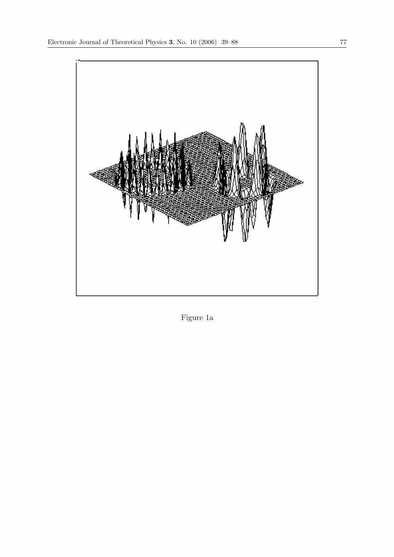
Electronic Journal of Theoretical Physics 3, No. 10 (2006) 39–88 77
Figure 1a
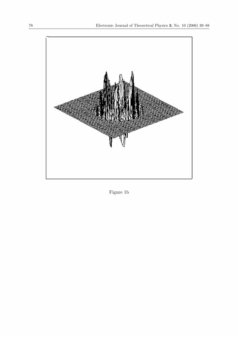
78 Electronic Journal of Theoretical Physics 3, No. 10 (2006) 39–88
Figure 1b
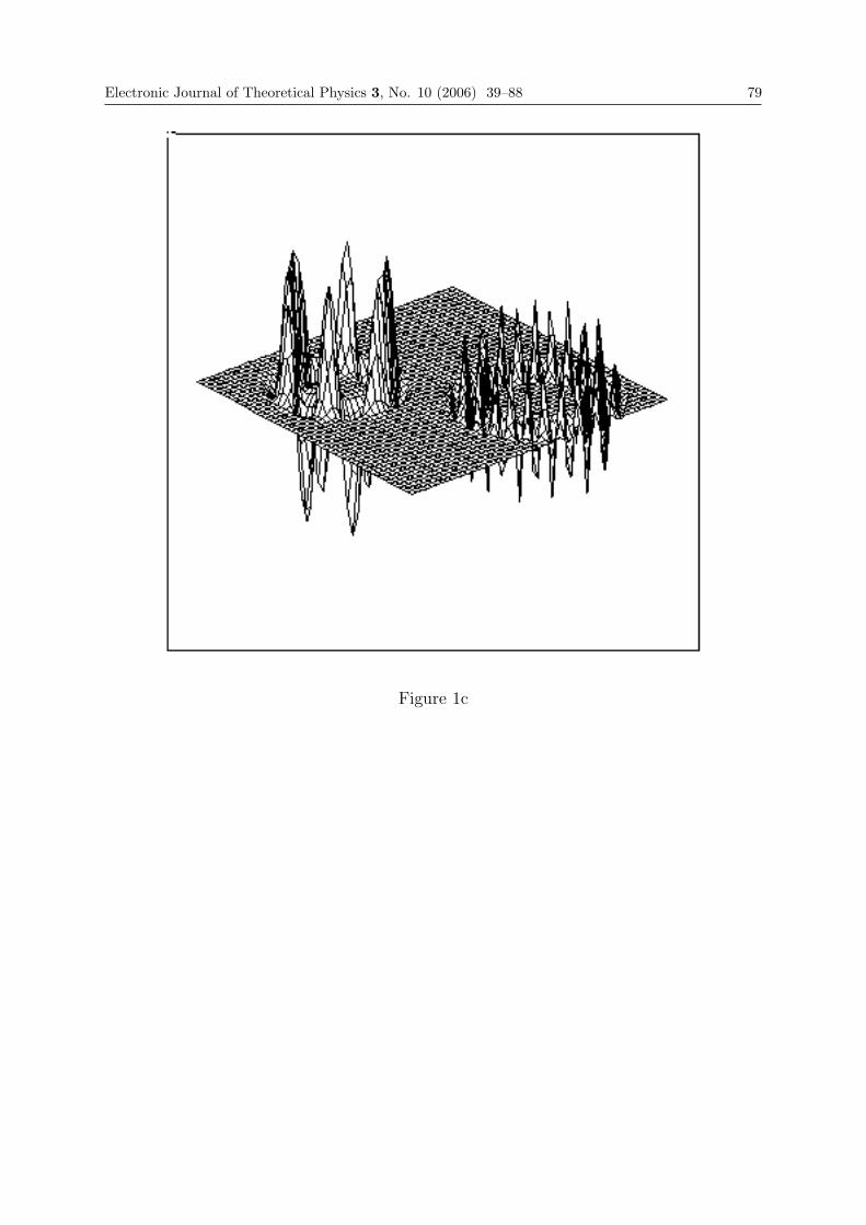
Electronic Journal of Theoretical Physics 3, No. 10 (2006) 39–88 79
Figure 1c
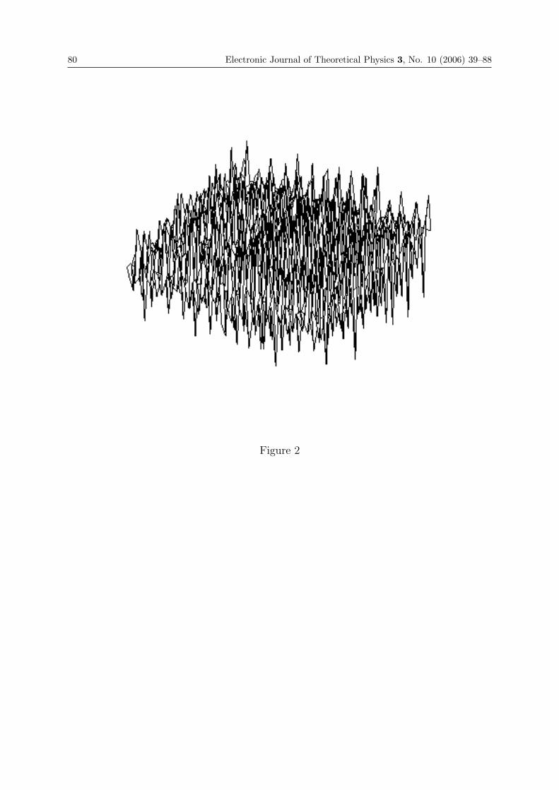
80 Electronic Journal of Theoretical Physics 3, No. 10 (2006) 39–88
Figure 2
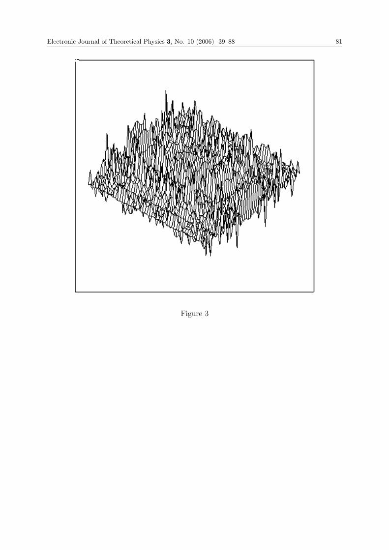
Electronic Journal of Theoretical Physics 3, No. 10 (2006) 39–88 81
Figure 3
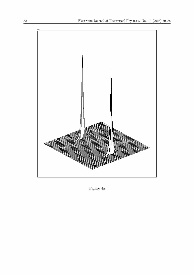
82 Electronic Journal of Theoretical Physics 3, No. 10 (2006) 39–88
Figure 4a
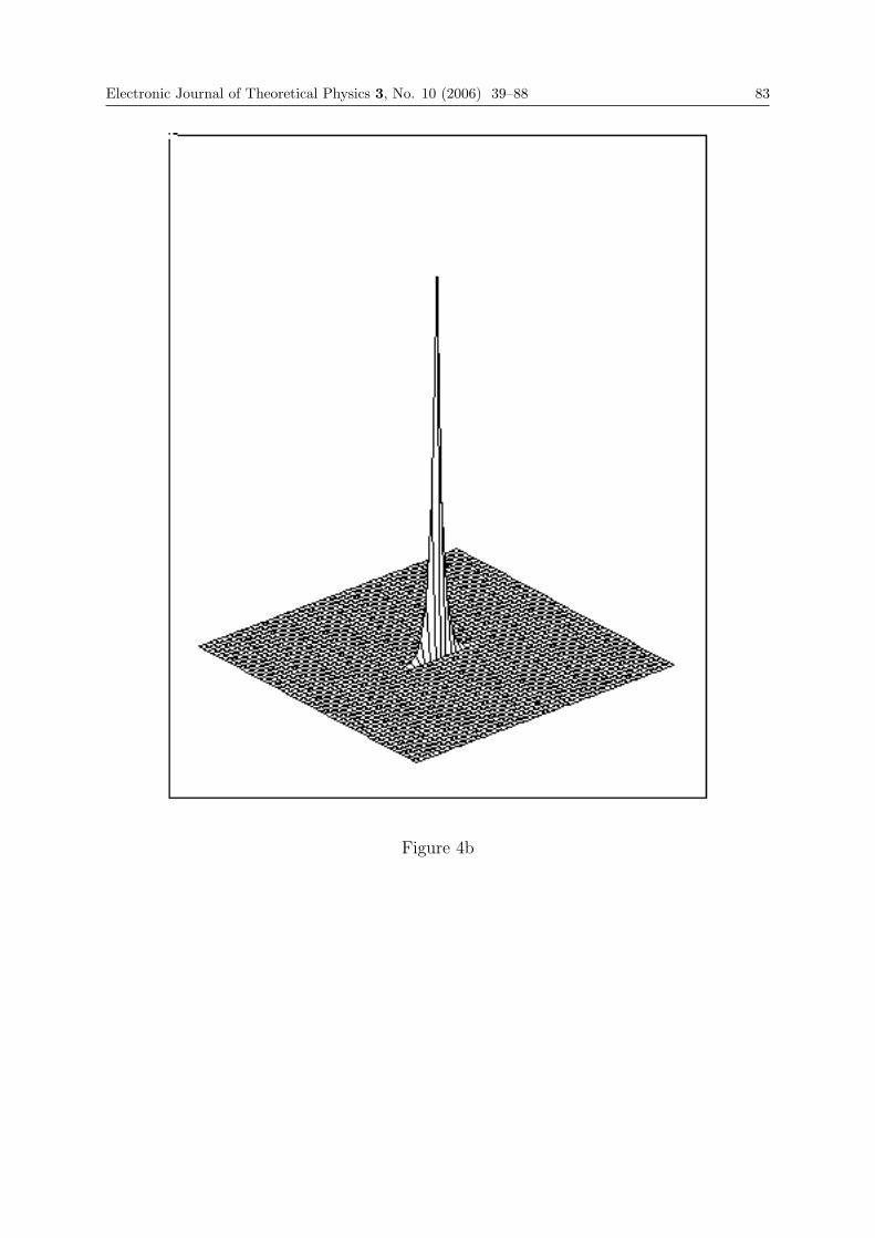
Electronic Journal of Theoretical Physics 3, No. 10 (2006) 39–88 83
Figure 4b
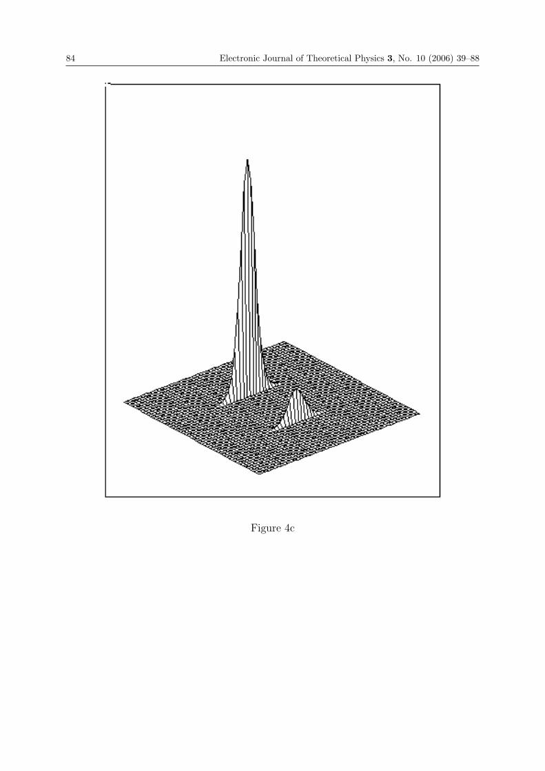
84 Electronic Journal of Theoretical Physics 3, No. 10 (2006) 39–88
Figure 4c
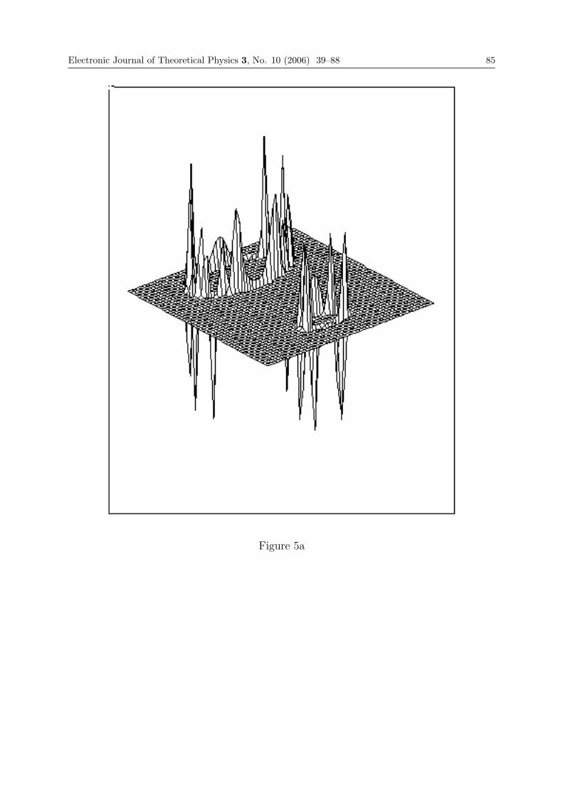
Electronic Journal of Theoretical Physics 3, No. 10 (2006) 39–88 85
Figure 5a
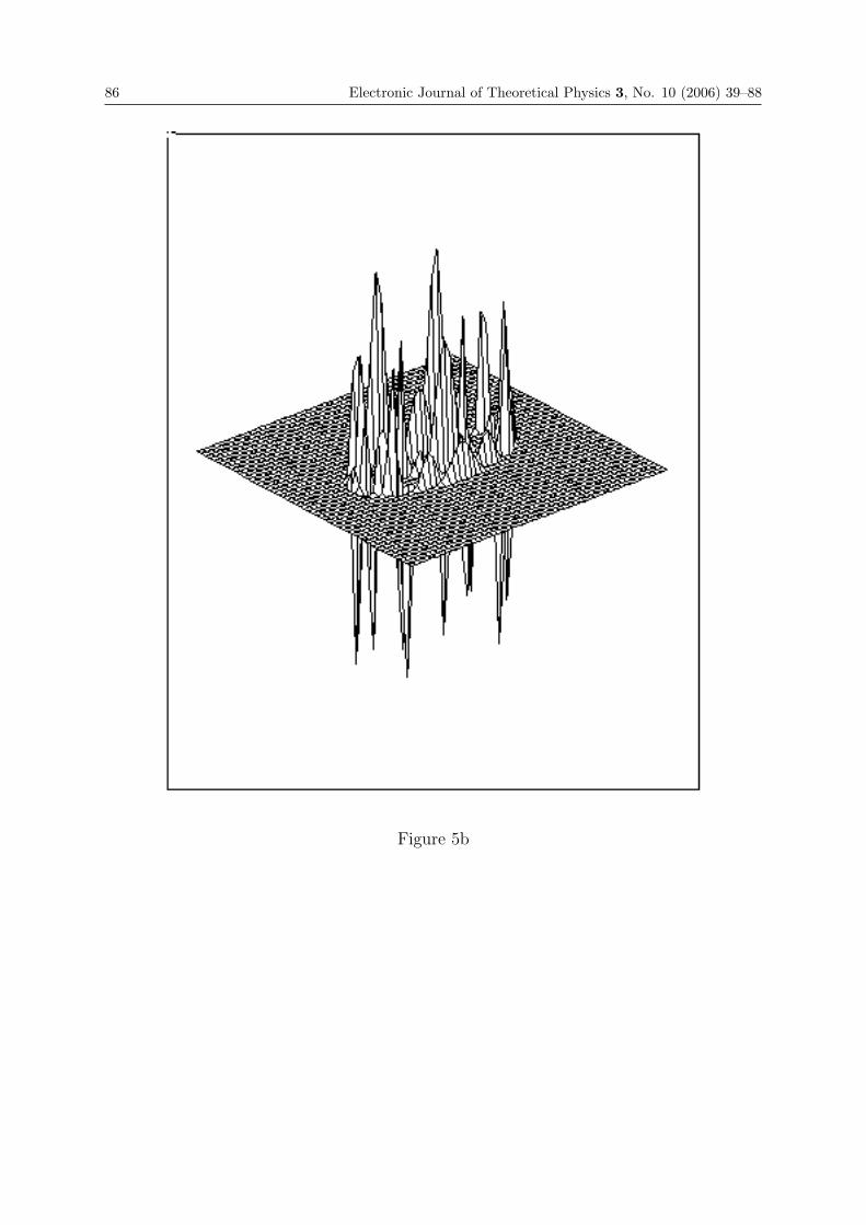
86 Electronic Journal of Theoretical Physics 3, No. 10 (2006) 39–88
Figure 5b
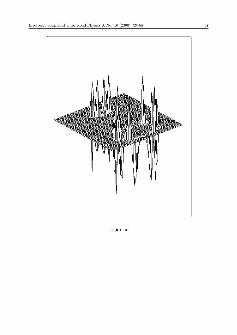
Electronic Journal of Theoretical Physics 3, No. 10 (2006) 39–88 87
Figure 5c
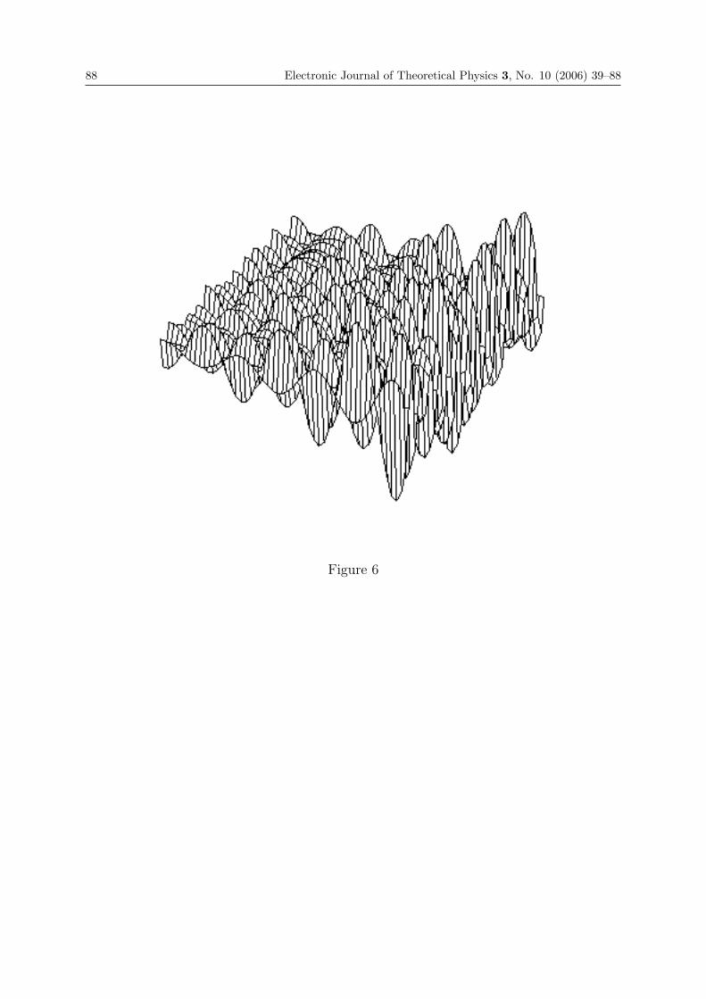
88 Electronic Journal of Theoretical Physics 3, No. 10 (2006) 39–88
Figure 6
EJTP 3, No. 10 (2006) 89–107 Electronic Journal of Theoretical Physics
The Quantum Character of Physical Fields.Foundations of Field Theories
L.I. Petrova ∗
Faculty of Computational Mathematics and Cybernetics,2nd Educational Building, Vorobjovy Gory,
Moscow State University,Moscow 119899, Russia
Received 10 March 2006, Published 28 May 2006
Abstract: The existing field theories are based on the properties of closed exterior forms, whichare invariant ones and correspond to conservation laws for physical fields. Hence, to understandthe foundations of field theories and their unity, one has to know how such closed exterior formsare obtained. In the present paper it is shown that closed exterior forms corresponding to fieldtheories are obtained from the equations modelling conservation (balance) laws for materialmedia. It has been developed the evolutionary method that enables one to describe the processof obtaining closed exterior forms. The process of obtaining closed exterior forms disclosesthe mechanism of evolutionary processes in material media and shows that material mediagenerate, discretely, the physical structures, from which the physical fields are formed. Thisjustifies the quantum character of field theories. On the other hand, this process demonstratesthe connection between field theories and the equations for material media and points to thefact that the foundations of field theories must be conditioned by the properties of materialmedia. It is shown that the external and internal symmetries of field theories are conditionedby the degrees of freedom of material media. The classification parameter of physical fields andinteractions, that is, the parameter of the unified field theory, is connected with the number ofnoncommutative balance conservation laws for material media.c© Electronic Journal of Theoretical Physics. All rights reserved.
Keywords: Foundations of Field Theories, Skew-Symmetric, Differential FormsPACS (2006): 11.10.Cd, 11.10.-z, 11.10.Jj, 11.30.-j, 03.65.Ta
Introduction
Originally, beginning from the 17th century, the physics based on the differential
equations, which describe physical processes. However, from the 20th century, the prob-
90 Electronic Journal of Theoretical Physics 3, No. 10 (2006) 89–107
lem of invariant (independent of the choice of the coordinate system) description of
physical phenomena arose. As the result, the formalisms based on the tensor, group,
variational methods, on the theories of symmetries, transformations and so on with the
basic requirement of invariance were developed in physics.
This gave rise to building the field theories that enable one to describe physical fields
and their interactions. Such theories were based on the postulates turned out practically
not to be connected with the equations of mathematical physics, which describe physical
processes. Just the absence of such a connection produced the emergence of the problems
in field theories that are connected with investigation of general foundations of existing
field theories, their unity, and constructing the general field theory.
In present paper it is shown that the connection of field theories with the equations
describing physical processes in material media must lie at the basis of the general field
theory.
The investigation of the foundations of field theories has been carried out using skew-
symmetric differential forms. Skew-symmetric differential forms, which deal with differ-
entials and differential expressions, can describe a conjugacy of various operators and
objects. This is of principal importance for mathematical physics and field theories since
the conjugated objects are invariants.
The properties of existing field theories are those of the closed exterior skew-symmetric
differential forms [1,2], which are conjugated objects and correspond to conservation laws
for physical fields. The properties of closed exterior forms explicitly or implicitly manifest
themselves essentially in all formalisms of field theory, such as the Hamilton formalism,
tensor approaches, group methods, quantum mechanics equations, the Yang-Mills theory
and others. The gauge transformations (unitary, gradient and so on), the gauge sym-
metries and the identical relations of field theories are transformations, symmetries and
relations of the theory of closed exterior forms.
Such connection between field theories and the theory of closed exterior forms enables
one to understand the properties of field theories, which are common for all existing field
theories.
However, this does not solve the basic problems of field theories. To understand
the general foundations of field theories and their unity, one must know how the closed
exterior forms connected with field theories are obtained.
It is known that the closed exterior forms are obtained from differential equations
provided the requirements of integrability of these equations [1].
In the present paper it is shown, firstly, that the equations describing (balance) con-
servation laws for material media serve as the differential equations from which the closed
exterior forms related to field theories and corresponding conservation laws for physical
fields are obtained. And, secondly, it is developed the method, which is evolutionary one
hence this method allows to find not only closed exterior forms, but also to describe the
process of obtaining closed exterior forms.
The process of obtaining closed exterior forms, on one side, demonstrates the con-
nection between field theories and the equations for material media, and, on other side,
Electronic Journal of Theoretical Physics 3, No. 10 (2006) 89–107 91
discloses the mechanism of evolutionary processes in material media and shows that ma-
terial media generate physical fields. This underlines the fact that the foundations of
field theories, namely, the theories describing physical fields, must be conditioned by the
properties of material media.
It has been possible to carry out the investigation of general foundations of field
theories due to the skew-symmetric differential forms, which, unlike to the exterior forms,
are defined on deforming manifolds and hence they possess the evolutionary properties.
The mathematical apparatus of such forms includes some nontraditional elements such as
nonidentical relations and degenerate transformation, and this enables one to describe the
evolutionary processes, discrete transitions, quantum jumps, and generation of various
structures.
In the first section the general properties of field theories are investigated with the help
of closed exterior forms. In the next section the analysis of the equations of the balance
conservation laws for material media, which describe the state of material system and the
mechanism of generating physical structures forming physical fields. In the last section
the general foundations of field theories obtained from the analysis of the equations for
material media are discussed.
1. Connection Of Field Theories with the Theory of Closed Ex-
terior Forms
Closed Exterior Forms and Conservation Laws
From the closure condition of the exterior form θp (p-form):
dθp = 0 (1.1)
one can see that the closed exterior form θp is a conserved quantity. This means that
this can correspond to a conservation law, namely, to some conservative quantity. If the
form is closed only on pseudostructure, i.e. this form is a closed inexact one, the closure
conditions are written as
dπθp = 0 (1.2)
dπ∗θp = 0 (1.3)
where ∗θp is the dual form.
Condition (1.3), i.e. the closure condition for dual form, specifies the pseudostructure
π. {Cohomology, sections of cotangent bundles, the eikonal surfaces, potential surfaces,
pseudo-Riemannian and pseudo-Euclidean spaces, and others are examples of the pseu-
dostructures and manifolds that are made up by pseudostructures.}From conditions (1.2) and (1.3) one can see the following. The dual form (pseudostruc-
ture) and closed inexact form (conservative quantity) made up a conjugated conservative
object that can also correspond to some conservation law. The conservation laws, to
which physical fields are subject, are just such conservation laws.
92 Electronic Journal of Theoretical Physics 3, No. 10 (2006) 89–107
The conservative object made up by the closed inexact exterior form and correspond-
ing dual form is a differential-geometrical structure. (Such differential-geometrical struc-
tures are examples of G-structures.) The physical structures, which made up physical
fields, and corresponding conservation laws are such differential-geometrical structures,
Properties of Closed Exterior Differential Forms
Invariance. Qauge transformations. It is known that the closed exact form is the
differential of the form of lower degree:
θp = dθp−1 (1.4)
Closed inexact form is also a differential, and yet not total but interior on pseudostructure
θpπ = dπθp−1 (1.5)
Since the closed form is a differential (a total one if the form is exact, or an interior
one on the pseudostructure if the form is inexact), it is obvious that the closed form turns
out to be invariant under all transformations that conserve the differential. The unitary
transformations, the tangent, the canonical, the gradient transformations and so on are
examples of such transformations. These are gauge transformations of field theories.
With the invariance of closed forms it is connected the covariance of relevant dual
forms.
Conjugacy. Duality. Symmetries. The closure of exterior differential forms is
the result of conjugating the elements of exterior or dual forms. The closure property
of the exterior form means that any objects, namely, the elements of exterior form, the
components of elements, the elements of the form differential, the exterior and dual forms,
the forms of sequential degrees and others, turn out to be conjugated.
With the conjugacy it is connected the duality.
The example of a duality having physical sense: the closed exterior form is a conserva-
tive quantity corresponding to conservation law, and the closed form (as the differential)
can correspond to a certain potential force.
The conjugacy is possible if there is one or another type of symmetry.
The gauge symmetries, which are interior symmetries of field theory and with which
gauge transformations are connected, are symmetries of closed exterior differential forms.
Symmetries of closed dual forms are exterior symmetries of the equations of field theory.
Identical relations of exterior forms. Since the conjugacy is a certain connec-
tion between two operators or mathematical objects, it is evident that, to express the
conjugacy mathematically, it can be used relations. These are identical relations.
The identical relations express the fact that each closed exterior form is the differential
of some exterior form (with the degree less by one). In general form such an identical
relation can be written as
dπϕ = θpπ (1.6)
Electronic Journal of Theoretical Physics 3, No. 10 (2006) 89–107 93
In this relation the form in the right-hand side has to be a closed one.
Identical relations of exterior differential forms are a mathematical expression of var-
ious types of conjugacy that leads to closed exterior forms.
Such relations like the Poincare invariant, vector and tensor identical relations, the
Cauchi-Riemann conditions, canonical relations, the integral relations by Stokes or Gauss-
Ostrogradskii, the thermodynamic relations, the eikonal relations, and so on are examples
of identical relations of closed exterior forms that have either the form of relation (1.6)
or its differential or integral analogs.
The Analysis of the Properties of Field Theories Using Closed Exterior
Forms
One can see that the properties of closed exterior differential forms correspond to the
properties of field theories. Hence, the mathematical principles of the theory of closed
exterior differential forms made up the basis of field theories that is common for all
existing field theories. (It should be emphasized that the field theories are connected
with the properties of inexact closed exterior forms.)
The connection between field theories and the theory of closed exterior forms is pri-
mary explained by the fact that the closure conditions of exterior and dual forms cor-
respond to conservation laws to which physical fields are subject. It is known that the
conservation laws for physical fields are those that state an existence of conservative phys-
ical quantities or objects. The physical structures, which made up physical fields, and
corresponding conservation laws are differential-geometrical structures formed by closed
exterior forms and dual ones. [Below, using the evolutionary forms it will be shown that
such physical structures arise in material media discretely.]
The properties of closed exterior and dual forms, namely, invariance, covariance, con-
jugacy, and duality, lie at the basis of the group, structural and other invariant methods
of field theories.
The nondegenerate transformations of field theory are transformations of closed exte-
rior forms. These are gauge transformations for spinor, scalar, vector, and tensor fields,
which are transformations of closed (0-form), (1-form), (2-form) and (3-form) respectively.
The gauge, i.e. internal, symmetries of the field theory equations (corresponding to
the gauge transformations) are those of closed exterior forms. The external symmetries
of the equations of field theory are symmetries of closed dual forms.
The basis of field theory operators is connected with the nondegenerate transforma-
tions of exterior differential forms. If, in addition to the exterior differential, we introduce
the following operators: (1) δ for transformations that convert the form of (p + 1) degree
into the form of p degree, (2) δ′ for cotangent transformations, (3) Δ for the dδ − δd
transformation, (4) Δ′ for the dδ′− δ′d transformation, one can write down the operators
in the field theory equations in terms of these operators that act on the exterior differ-
ential forms. The operator δ corresponds to Green’s operator, δ′ does to the canonical
transformation operator, Δ does to the d’Alembert operator in 4-dimensional space, and
94 Electronic Journal of Theoretical Physics 3, No. 10 (2006) 89–107
Δ′ corresponds to the Laplace operator.
It can be shown that the equations of existing field theories are those obtained on the
basis of the properties of the exterior form theory. The Hamilton formalism is based on
the properties of closed exterior form of the first degree and corresponding dual form. The
closed exterior differential form ds = −Hdt+pjdqj (the Poincare invariant) corresponds to
the field equation related to the Hamilton system. The Schrodinger equation in quantum
mechanics is an analog to field equation, where the conjugated coordinates are changed
by operators. It is evident that the closed exterior form of zero degree (and dual form)
correspond to quantum mechanics. Dirac’s bra- and cket- vectors constitute a closed
exterior form of zero degree [3]. The properties of closed exterior form of the second
degree (and dual form) lie at the basis of the electromagnetic field equations. The Maxwell
equations may be written as [4] dθ2 = 0, d∗θ2 = 0, where θ2 = 12Fμνdxμdxν (here Fμν is
the strength tensor). Closed exterior and dual forms of the third degree correspond to
the gravitational field. (However, to the physical field of given type it can be assigned
closed forms of less degree. In particular, to the Einstein equation [5] for gravitational
field it is assigned the first degree closed form, although it was pointed out that the type
of a field with the third degree closed form corresponds to the gravitational field.)
One can recognize that the gauge transformations as well as the symmetries and
equations of field theories are connected with closed exterior forms of given degree. This
enables one to introduce a classification of physical fields and interactions according to
the degree of closed exterior form. (If denote the degree of corresponding closed exterior
forms by k, the case k = 0 will correspond to strong interaction, k = 1 will correspond
to weak interaction, k = 2 will correspond to electromagnetic interaction, and k = 3
will correspond to gravitational interaction.) This shows that there exists a commonness
between field theories describing physical fields of different types. The degree of closed
exterior forms is a parameter that integrates fields theories into unified field theory.
Thus one can see that existing invariant field theories are based on the properties
of closed exterior forms. And such a connection also discloses the problems of existing
invariant field theories.
There are no answer to the question of how closed inexact exterior forms, which
correspond to physical structures and reflect the properties of conservation laws and on
which properties field theories are based, are obtained.
Below we will show that the answer to these question may be obtained from the anal-
ysis of differential equations describing the conservation laws for material media. These
are just the equations from which the closed exterior forms whose properties correspond
to field theories are obtained.
The evolutionary method of investigating these equations applied in the present paper
enables one to understand how physical fields are formed and what must lie at the basis
of the general field theory. [The method that enables one to find the closed exterior forms (the
invariants) had been proposed by Cartan [1]. The differential equations are imposed by the requirement
of obeying the closure condition of exterior form made up by the derivatives of these equations (it is
added the requirement that the external form differential vanishes), and next one finds the conditions
Electronic Journal of Theoretical Physics 3, No. 10 (2006) 89–107 95
that these requirements are satisfied (the integrability conditions). This method enables one to find the
closed exterior forms (the invariants) that can possess the equation under consideration. However, for
the evolutionary equations of mathematical physics describing physical processes it is important not only
to find closed forms, but it is also important to know how these forms are obtained, in other words, it
is important to know how the closure conditions of exterior forms are realized evolutionary. For this a
principally new evolutionary method is necessary.]
2. The Equations of Balance Conservation Laws for Material
System: The Evolutionary Processes in Material Media. Orig-
ination of Physical Structures
The conservation laws for material media (material media will be considered as
material systems) are the balance conservation laws for energy, linear momentum, angular
momentum, and mass. They are described by differential equations [6-8]. [Material system
is a variety of elements that have internal structure and interact to one another. Thermodynamic and
gas dynamical systems, systems of charged particles, cosmic systems, systems of elementary particles
and others are examples of material systems. Examples of elements that constitute the material system
are electrons, protons, neutrons, atoms, fluid particles, cosmic objects and others. The conservation laws
for material systems are balance ones. These are conservation laws that establish a balance between the
variation of physical quantity of material system and the corresponding external action.]
Nonconjugacy of the Balance Conservation Law Equations: Noncommu-
tativity of the Balance Conservation Laws
The conservation laws for material systems have a peculiarity, namely, they are non-
commutative ones. To this it points out the analysis of the equations of the balance
conservation laws. (Just the noncommutativity of the balance conservation laws is a
moving force of the evolutionary processes in material media that lead to generation of
physical fields.)
It turns out that, even without a knowledge of the concrete form of the equations for
balance conservation laws, with the help of skew-symmetric differential forms one can see
their specific features. To carry out such an investigation, in addition to exterior skew-
symmetric forms the skew-symmetric differential forms, which possesses the evolutionary
properties (and for this reason the author named those as ”evolutionary” ones), will be
used. These are skew-symmetric differential forms, which, unlike to exterior forms, are
defined on deforming manifolds. Such skew-symmetric differential forms have a specific
feature, namely, they cannot be closed. The differential of such form does not vanish. This
differential includes the metric form differential of deforming manifold, which is obtained
due to differentiating the basis and is nonzero. The evolutionary form commutator, in
addition to the commutator made up by the derivatives of the coefficients of the form
itself, includes (in contrast to the commutator of the exterior form) the metric form
96 Electronic Journal of Theoretical Physics 3, No. 10 (2006) 89–107
commutator being nonzero.
(The role of evolutionary forms in mathematical physics and field theory is due to the
fact that they, as well as exterior forms, correspond to conservation laws. However, these
conservation laws are those not for physical fields but for material media.)
We will analyze the equations that describe the balance conservation laws for energy
and linear momentum.
If firstly to write down these equations in the inertial reference system and next pass to
the accompanying reference system (this system is connected with the manifold built by
the trajectories of the material system elements), in the accompanying reference system
the energy equation will be written in the form
∂ψ
∂ξ1= A1 (2.1)
Here ψ is the functional specifying the state of material system (the action functional,
entropy or wave function can be regarded as examples of such a functional), ξ1 is the
coordinate along the trajectory, A1 is the quantity that depends on specific features of
material system and on external (with respect to local domain made up by the element
and its neighborhood) energy actions onto the system.
In a similar manner, in the accompanying reference system the equation for linear
momentum appears to be reduced to the equation of the form
∂ψ
∂ξν= Aν , ν = 2, ... (2.2)
where ξν are the coordinates in the direction normal to the trajectory, Aν are the quanti-
ties that depend on the specific features of material system and on external force actions.
Eqs. (2.1) and (2.2) can be convoluted into the relation
dψ = Aμ dξμ, (μ = 1, ν) (2.3)
where dψ is the differential expression dψ = (∂ψ/∂ξμ)dξμ.
Relation (2.3) can be written as
dψ = ω (2.4)
here ω = Aμ dξμ is the skew-symmetric differential form of the first degree.
Since the balance conservation laws are evolutionary ones, the relation obtained is
also an evolutionary relation.
Relation (2.4) was obtained from the equation of the balance conservation laws for
energy and linear momentum. In this relation the form ω is that of the first degree. If
the equations of the balance conservation laws for angular momentum be added to the
equations for energy and linear momentum, this form in the evolutionary relation will
be a form of the second degree. And in combination with the equation of the balance
conservation law for mass this form will be a form of degree 3.
Electronic Journal of Theoretical Physics 3, No. 10 (2006) 89–107 97
Thus, in general case the evolutionary relation can be written as
dψ = ωp (2.5)
where the form degree p takes the values p = 0, 1, 2, 3. The evolutionary relation for
p = 0 is similar to that in the differential forms, and it was obtained from the interaction
of time and energy of material system.
It could be noted that the degree p is connected with the number of interacting
conservation laws that is equal to (p + 1).
Relation obtained from the equation of the balance conservation laws has a specific
feature, namely, this relation turns out to be nonidentical.
To justify this we shall analyze relation (2.4). This relation proves to be nonidentical
since the left-hand side of the relation is a differential, which is a closed form, but the right-
hand side of the relation involves the differential form ω, which is unclosed evolutionary
form. The metric form commutator of the manifold, on which the form ω is defined, is
nonzero since this manifold is an accompanying, deforming, manifold. The commutator
made up by the derivatives of coefficients Aμ the form ω itself is also nonzero, since the
coefficients Aμ are of different nature, that is, some coefficients have been obtained from
the energy equation and depend on the energetic actions, whereas the others have been
obtained from the equation for linear momentum and depend on the force actions.
In a similar manner one can prove the nonidentity of relation (2.5).
The nonidentity of evolutionary relation means that the balance conservation law
equations are inconsistent (nonconjugated). This reflects the properties of the balance
conservation laws that have a governing importance for the evolutionary processes in ma-
terial media, namely, their noncommutativity. [The nonidentity of evolutionary relation points
to the fact that on the initial manifold the equations of the balance conservation laws are nonintegrable
ones: the derivatives of these equations do not make up the differential, that is, a closed form which can
be directly integrated. This is explained by the fact that these equations, like any equations describing
physical processes, include nonpotential terms.]
Physical Meaning of the Equations of Balance Conservation Laws: De-
scription of the State of Material System
Nonequilibrium state of material system. The evolutionary relation obtained from
the equations of balance conservation laws discloses a physical meaning of these equations
– these equations describe the state of material system.
It is evident that if the balance conservation laws be commutative, the evolutionary
relation would be identical and from that it would be possible to get the differential dψ,
this would indicate that the material system is in the equilibrium state.
However, as it has been shown, in real processes the balance conservation laws are
noncommutative. The evolutionary relation is not identical and from this relation one
cannot get the differential dψ. This means that the system state is nonequilibrium. That
98 Electronic Journal of Theoretical Physics 3, No. 10 (2006) 89–107
is, due to noncommutativity of the balance conservation laws the material system state
turns out to be nonequilibrium. It is evident that the internal force producing such
nonequilibrium state is described by the evolutionary form commutator. Everything that
gives the contribution to the commutator of the form ωp leads to emergence of internal
force. (Internal force is a force that acts inside the local domain of material system, i.e.
a domain made up by the element and its neighborhood.)
Nonidentical evolutionary relation also describes how the state of material system
varies. This turns out to be possible due to the fact that the evolutionary nonidentical
relation is a selfvarying one. This relation includes two objects one of which appears
to be unmeasurable. The variation of any object of the relation in some process leads
to variation of another object and, in turn, the variation of the latter leads to variation
of the former. Since one of the objects is an unmeasurable quantity, the other cannot
be compared with the first one, and hence, the process of mutual variation cannot stop.
This process is governed by the evolutionary form commutator, that is, by interaction
between the commutator made up by derivatives of the form itself and by metric form
commutator of deforming manifold made up by the trajectories of material system. (This
is an exchange between quantities of different nature, between physical quantities and
space-time characteristics.)
[In essence, the evolutionary equation is a correlative relation. When changing the terms of this
relation cannot become equal to one another, but in this case they correlate to one another. The terms
of the evolutionary form commutator in nonidentical relation also correlate to one another.]
Selfvariation of nonidentical evolutionary relation points to the fact that the nonequi-
librium state of material system turns out to be selfvarying. State of material system
changes but holds nonequilibrium during this process.
Transition of material system from nonequilibrium state to the locally-
equilibrium state. Origination of physical structure. The significance of the
evolutionary relation selfvariation consists in the fact that in such a process it can be
realized conditions under which the inexact, closed on pseudostructure, exterior form is
obtained from the evolutionary form. This transition is possible only as the degenerate
transformation, namely, a transformation that does not conserve the differential. The
conditions of degenerate transformation are those that determine the direction on which
interior (only along a given direction) differential of the evolutionary form vanishes. These
are the conditions that defines the pseudostructure, i.e. the closure conditions of dual
form, and leads to realization of the exterior form closed on pseudostructure.
As it has been already mentioned, the differential of the evolutionary form ωp involved
into nonidentical relation (2.5) is nonzero. That is,
dωp �= 0 (2.6)
If the conditions of degenerate transformation are realized, it will take place the transition
dωp �= 0→ (degenerate transformation) → dπωp = 0, dπ∗ωp = 0
The relations obtained
dπωp = 0, dπ∗ωp = 0 (2.7)
Electronic Journal of Theoretical Physics 3, No. 10 (2006) 89–107 99
are the closure conditions for exterior inexact form and dual form. This means that it is
realized the exterior form closed on pseudostructure.
In this case on the pseudostructure π evolutionary relation (2.5) converts into the
relation
dπψ = ωpπ (2.8)
which proves to be an identical relation. Since the form ωpπ is a closed one, on the
pseudostructure this form turns out to be a differential. There are differentials in the
left-hand and right-hand sides of this relation. This means that the relation obtained is
an identical one.
Here it should be emphasized that under degenerate transformation the evolutionary
form remains to be unclosed and the evolutionary relation itself remains to be nonidentical
one. (The evolutionary form differential vanishes only on pseudostructure: the differen-
tial, which equals zero, is an interior one, the total differential of the evolutionary form
is nonzero.)
The transition from nonidentical relation (2.5) obtained from the balance conservation
laws to identical relation (2.8) means the following. Firstly, the emergence of the closed
(on pseudostructure) inexact exterior form (relation (2.7) and right-hand side of relation
(2.8)) points to origination of physical structure. And, secondly, the existence of the state
differential (left-hand side of relation (2.8)) points to the transition of material system
from nonequilibrium state to the locally-equilibrium state. (But in this case the total
state of the material system turns out to be nonequilibrium.)
Identical relation (2.8) points to the fact that the origination of physical structures is
connected with the transition of material system to the locally-equilibrium state.
The origination of physical structures in material system manifests itself as an emer-
gence of certain observable formations, which develop spontaneously. Such formations
and their manifestations are fluctuations, turbulent pulsations, waves, vortices, creating
massless particles, and others. (One can see that the processes described also explain
such phenomena as turbulence, radiation and others.)
Conditions of degenerate transformation: degrees of freedom of material
system. The conditions of degenerate transformation that lead to emergence of closed
inexact exterior form are connected with any symmetries. Since these conditions are
closure conditions of dual (metric) form, they can be caused by symmetries of coefficients
of the metric form commutator (for example, these can be symmetrical connectednesses).
Under describing material system the symmetries are conditioned by degrees of free-
dom of material system. The translational degrees of freedom, internal degrees of freedom
of the system elements, and so on can be examples of such degrees of freedom.
The conditions of degenerate transformation (vanishing the dual form commutator)
define the pseudostructure. These conditions specify the derivative of implicit function,
which defines the direction of pseudostructure. The speeds of various waves are examples
of such derivatives: the speed of light, the speed of sound and of electromagnetic waves,
the speed of creating particles and so on. It can be shown that the equations for surfaces
100 Electronic Journal of Theoretical Physics 3, No. 10 (2006) 89–107
of potential (of simple layer, double layer), integral surfaces, equations for one, two, . . .
eikonals, of the characteristic and of the characteristic surfaces, the residue equations and
so on serve as the equations for pseudostructures.
To the degenerate transformation it must correspond a vanishing of some functional
expressions, such as Jacobians, determinants, the Poisson brackets, residues and others.
Vanishing of these functional expressions is the closure condition for dual form.
And it should be emphasized once more that the degenerate transformation is realized
as a transition from the accompanying noninertial coordinate system to the locally inertial
system. The evolutionary form is defined in the noninertial frame of reference (deforming
manifold). But the closed exterior form created is obtained with respect to the locally-
inertial frame of reference (pseudostructure).
Characteristics and Classification of Physical Structures. Forming Pseu-
dometric and Metric Spaces
Characteristics of physical structures. The physical structure is a differential-
geometrical structure made up by the dual form and closed inexact form. This is a
pseudostructure (dual form) with conservative quantity (closed inexact form). The con-
servative quantities describe certain charges.
Since the physical structures are generated by material media by means of the balance
conservation laws, their characteristics are connected with the characteristics of material
systems and with the characteristics of evolutionary forms obtained from the equations
of balance conservation laws.
It was already mentioned that the pseudostructure is obtained from the condition of
degenerate transformation, which is connected with the degrees of freedom of material
system.
The total differential of evolutionary form, which holds to be nonzero, defines two
another characteristics of physical structure.
The first term of the evolutionary form differential, more exactly, its commutator,
determines the value of discrete change (the quantum), which the quantity conserved on
the pseudostructure undergoes during transition from one pseudostructure to another.
The second term of the evolutionary form commutator determines the bending of pseu-
dostructure. The bending specifies the characteristics that fixes the character of the
manifold deformation, which took place before physical structure emerged. (Spin is an
example of such a characteristics).
The closed exterior forms obtained correspond to the state differential for material
system. The differentials of entropy, action, potential and others are examples of such
differentials.
As it was already mentioned, in material system the created physical structure is
revealed as an observable formation. It is evident that the characteristics of the formation
(intensity, vorticity, absolute and relative speeds of propagation of the formation), as well
as those of created physical structure, are determined by the evolutionary form and its
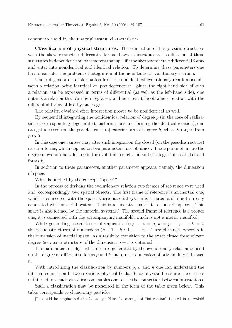
Electronic Journal of Theoretical Physics 3, No. 10 (2006) 89–107 101
commutator and by the material system characteristics.
Classification of physical structures. The connection of the physical structures
with the skew-symmetric differential forms allows to introduce a classification of these
structures in dependence on parameters that specify the skew-symmetric differential forms
and enter into nonidentical and identical relation. To determine these parameters one
has to consider the problem of integration of the nonidentical evolutionary relation.
Under degenerate transformation from the nonidentical evolutionary relation one ob-
tains a relation being identical on pseudostructure. Since the right-hand side of such
a relation can be expressed in terms of differential (as well as the left-hand side), one
obtains a relation that can be integrated, and as a result he obtains a relation with the
differential forms of less by one degree.
The relation obtained after integration proves to be nonidentical as well.
By sequential integrating the nonidentical relation of degree p (in the case of realiza-
tion of corresponding degenerate transformations and forming the identical relation), one
can get a closed (on the pseudostructure) exterior form of degree k, where k ranges from
p to 0.
In this case one can see that after such integration the closed (on the pseudostructure)
exterior forms, which depend on two parameters, are obtained. These parameters are the
degree of evolutionary form p in the evolutionary relation and the degree of created closed
forms k.
In addition to these parameters, another parameter appears, namely, the dimension
of space.
What is implied by the concept “space”?
In the process of deriving the evolutionary relation two frames of reference were used
and, correspondingly, two spatial objects. The first frame of reference is an inertial one,
which is connected with the space where material system is situated and is not directly
connected with material system. This is an inertial space, it is a metric space. (This
space is also formed by the material systems.) The second frame of reference is a proper
one, it is connected with the accompanying manifold, which is not a metric manifold.
While generating closed forms of sequential degrees k = p, k = p − 1, . . . , k = 0
the pseudostructures of dimensions (n + 1 − k): 1, . . . , n + 1 are obtained, where n is
the dimension of inertial space. As a result of transition to the exact closed form of zero
degree the metric structure of the dimension n + 1 is obtained.
The parameters of physical structures generated by the evolutionary relation depend
on the degree of differential forms p and k and on the dimension of original inertial space
n.
With introducing the classification by numbers p, k and n one can understand the
internal connection between various physical fields. Since physical fields are the carriers
of interactions, such classification enables one to see the connection between interactions.
Such a classification may be presented in the form of the table given below. This
table corresponds to elementary particles.
[It should be emphasized the following. Here the concept of “interaction” is used in a twofold
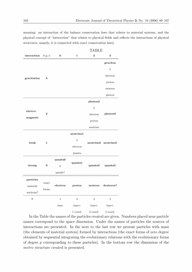
102 Electronic Journal of Theoretical Physics 3, No. 10 (2006) 89–107
meaning: an interaction of the balance conservation laws that relates to material systems, and the
physical concept of “interaction” that relates to physical fields and reflects the interactions of physical
structures, namely, it is connected with exact conservation laws].
TABLEinteraction k\p, n 0 1 2 3
gravitation 3
graviton
⇑
electron
proton
neutron
photon
electro-
magnetic
2
photon2
⇑
electron
proton
neutrino
photon3
weak 1
neutrino1
⇑
electron
quanta
neutrino2 neutrino3
strong 0
quanta0
⇑
quarks?
quanta1quanta2 quanta3
particles
material
nucleons?
exact
forms
electron proton neutron deuteron?
N 1 2 3 4
time time+ time+ time+
1 coord. 2 coord. 3 coord.
In the Table the names of the particles created are given. Numbers placed near particle
names correspond to the space dimension. Under the names of particles the sources of
interactions are presented. In the next to the last row we present particles with mass
(the elements of material system) formed by interactions (the exact forms of zero degree
obtained by sequential integrating the evolutionary relations with the evolutionary forms
of degree p corresponding to these particles). In the bottom row the dimension of the
metric structure created is presented.
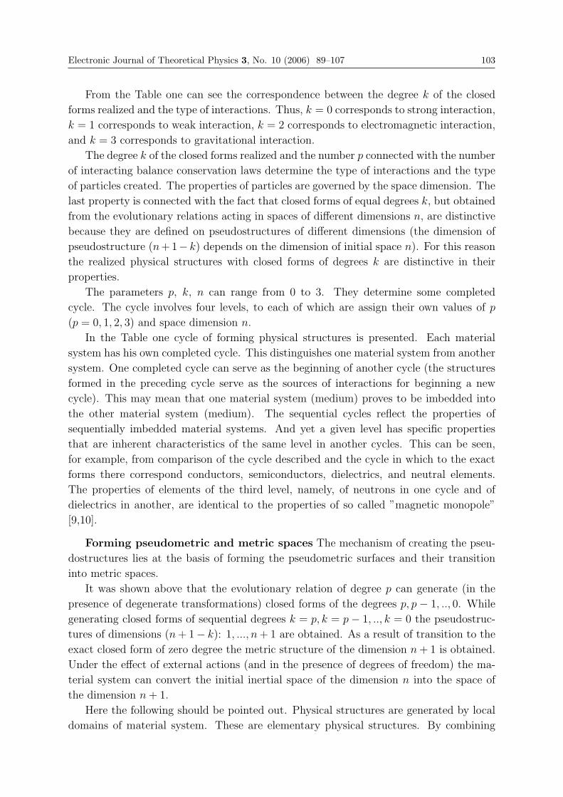
Electronic Journal of Theoretical Physics 3, No. 10 (2006) 89–107 103
From the Table one can see the correspondence between the degree k of the closed
forms realized and the type of interactions. Thus, k = 0 corresponds to strong interaction,
k = 1 corresponds to weak interaction, k = 2 corresponds to electromagnetic interaction,
and k = 3 corresponds to gravitational interaction.
The degree k of the closed forms realized and the number p connected with the number
of interacting balance conservation laws determine the type of interactions and the type
of particles created. The properties of particles are governed by the space dimension. The
last property is connected with the fact that closed forms of equal degrees k, but obtained
from the evolutionary relations acting in spaces of different dimensions n, are distinctive
because they are defined on pseudostructures of different dimensions (the dimension of
pseudostructure (n+1− k) depends on the dimension of initial space n). For this reason
the realized physical structures with closed forms of degrees k are distinctive in their
properties.
The parameters p, k, n can range from 0 to 3. They determine some completed
cycle. The cycle involves four levels, to each of which are assign their own values of p
(p = 0, 1, 2, 3) and space dimension n.
In the Table one cycle of forming physical structures is presented. Each material
system has his own completed cycle. This distinguishes one material system from another
system. One completed cycle can serve as the beginning of another cycle (the structures
formed in the preceding cycle serve as the sources of interactions for beginning a new
cycle). This may mean that one material system (medium) proves to be imbedded into
the other material system (medium). The sequential cycles reflect the properties of
sequentially imbedded material systems. And yet a given level has specific properties
that are inherent characteristics of the same level in another cycles. This can be seen,
for example, from comparison of the cycle described and the cycle in which to the exact
forms there correspond conductors, semiconductors, dielectrics, and neutral elements.
The properties of elements of the third level, namely, of neutrons in one cycle and of
dielectrics in another, are identical to the properties of so called ”magnetic monopole”
[9,10].
Forming pseudometric and metric spaces The mechanism of creating the pseu-
dostructures lies at the basis of forming the pseudometric surfaces and their transition
into metric spaces.
It was shown above that the evolutionary relation of degree p can generate (in the
presence of degenerate transformations) closed forms of the degrees p, p − 1, .., 0. While
generating closed forms of sequential degrees k = p, k = p− 1, .., k = 0 the pseudostruc-
tures of dimensions (n + 1− k): 1, ..., n + 1 are obtained. As a result of transition to the
exact closed form of zero degree the metric structure of the dimension n + 1 is obtained.
Under the effect of external actions (and in the presence of degrees of freedom) the ma-
terial system can convert the initial inertial space of the dimension n into the space of
the dimension n + 1.
Here the following should be pointed out. Physical structures are generated by local
domains of material system. These are elementary physical structures. By combining
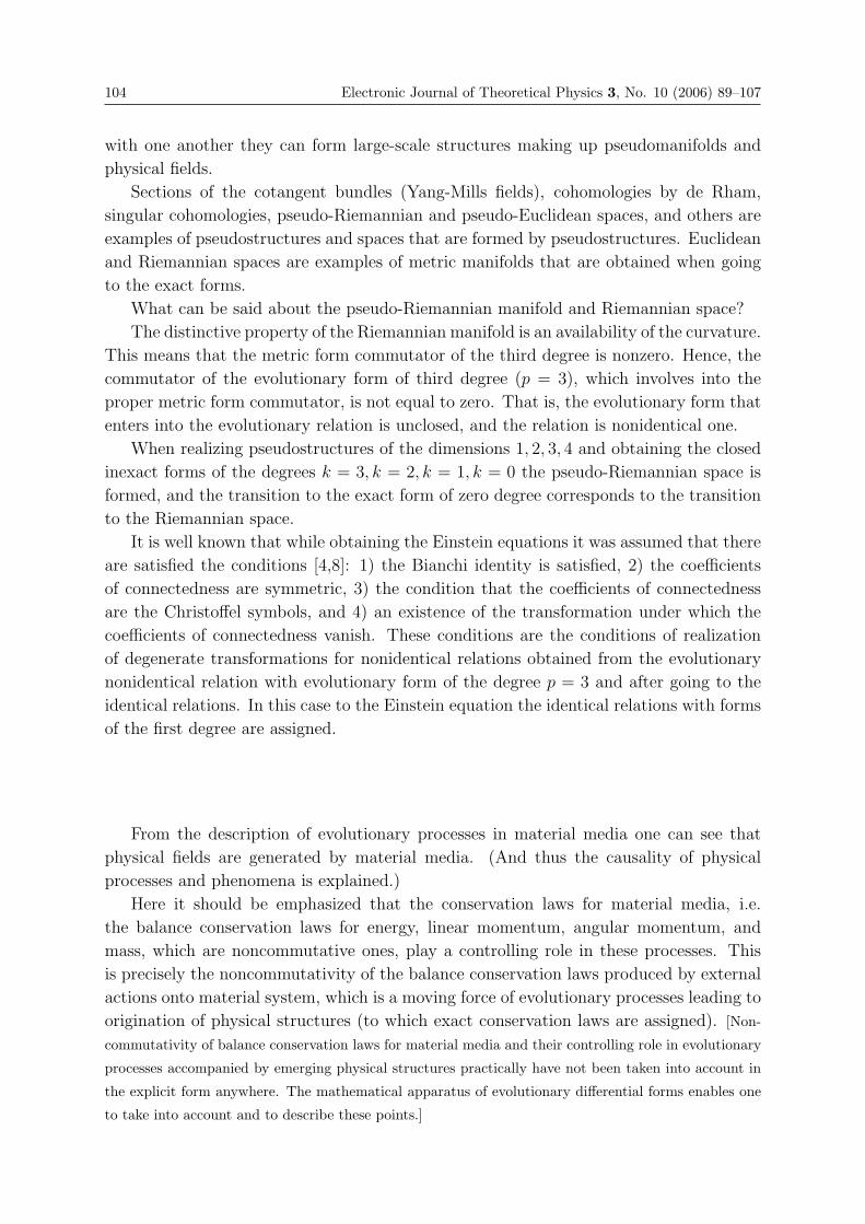
104 Electronic Journal of Theoretical Physics 3, No. 10 (2006) 89–107
with one another they can form large-scale structures making up pseudomanifolds and
physical fields.
Sections of the cotangent bundles (Yang-Mills fields), cohomologies by de Rham,
singular cohomologies, pseudo-Riemannian and pseudo-Euclidean spaces, and others are
examples of pseudostructures and spaces that are formed by pseudostructures. Euclidean
and Riemannian spaces are examples of metric manifolds that are obtained when going
to the exact forms.
What can be said about the pseudo-Riemannian manifold and Riemannian space?
The distinctive property of the Riemannian manifold is an availability of the curvature.
This means that the metric form commutator of the third degree is nonzero. Hence, the
commutator of the evolutionary form of third degree (p = 3), which involves into the
proper metric form commutator, is not equal to zero. That is, the evolutionary form that
enters into the evolutionary relation is unclosed, and the relation is nonidentical one.
When realizing pseudostructures of the dimensions 1, 2, 3, 4 and obtaining the closed
inexact forms of the degrees k = 3, k = 2, k = 1, k = 0 the pseudo-Riemannian space is
formed, and the transition to the exact form of zero degree corresponds to the transition
to the Riemannian space.
It is well known that while obtaining the Einstein equations it was assumed that there
are satisfied the conditions [4,8]: 1) the Bianchi identity is satisfied, 2) the coefficients
of connectedness are symmetric, 3) the condition that the coefficients of connectedness
are the Christoffel symbols, and 4) an existence of the transformation under which the
coefficients of connectedness vanish. These conditions are the conditions of realization
of degenerate transformations for nonidentical relations obtained from the evolutionary
nonidentical relation with evolutionary form of the degree p = 3 and after going to the
identical relations. In this case to the Einstein equation the identical relations with forms
of the first degree are assigned.
From the description of evolutionary processes in material media one can see that
physical fields are generated by material media. (And thus the causality of physical
processes and phenomena is explained.)
Here it should be emphasized that the conservation laws for material media, i.e.
the balance conservation laws for energy, linear momentum, angular momentum, and
mass, which are noncommutative ones, play a controlling role in these processes. This
is precisely the noncommutativity of the balance conservation laws produced by external
actions onto material system, which is a moving force of evolutionary processes leading to
origination of physical structures (to which exact conservation laws are assigned). [Non-
commutativity of balance conservation laws for material media and their controlling role in evolutionary
processes accompanied by emerging physical structures practically have not been taken into account in
the explicit form anywhere. The mathematical apparatus of evolutionary differential forms enables one
to take into account and to describe these points.]
Electronic Journal of Theoretical Physics 3, No. 10 (2006) 89–107 105
3. On the Foundations of General Field Theory
The results of the analysis of the equations of conservation laws for material media shows
the connection of physical fields with material media.
This points to the fact that the fields theories that describe physical fields must be
connected with the equations that describe material systems.
Such a connection, which is common to all field theories, discloses the general foun-
dations of field theories, their quantum character, justifies the unity of field theories and
can serve as an approach to general field theory.
The theories of exterior and evolutionary skew-symmetric differential forms, which
reflect the properties of conservation laws for physical fields and material media, allow to
disclose and justify the general principles of field theories. In this case the properties of
closed exterior forms demonstrate these principles, and the theory of evolutionary forms
justifies this. Below we present certain of concepts that lie at the basis of field theories.
(The results obtained with using the evolutionary forms are italicized).
1. Physical fields are formatted by physical structures that are described by closed
inexact exterior and dual forms. Physical structures are generated by material media.
Characteristics of physical structures relate to the characteristics of material systems.
2. The conservation laws for physical fields, on which the field theories are based, are
connected with the conservation laws for material media (with the balance conservation
laws for energy, linear momentum, angular momentum, and mass and the analog of such
law for the time).
3. Internal and external symmetries of field theories are those of closed exterior and
dual forms. They are conditioned by the degrees of freedom of material media.
4. The origination of physical structures, from which physical fields are made up,
proceeds discretely under realization of the degrees of freedom of material systems. This
explains the quantum character of field theories.
5. The gauge transformations of field theories are transformations of closed exte-
rior forms. They are connected with the degenerate transformations of the equations of
conservation laws for material media.
6. The constants of field theory must be connected with the characteristics of material
systems.
7. The classification parameter of physical fields and interactions, that is, the pa-
rameter of the unified field theory, is the degree of closed exterior forms corresponding
to conservation laws for physical fields. This parameter is connected with the number of
the equations of interacting noncommutative balance conservation laws. This connection
justifies the parameter of the united field theory.
The results obtained show that when building the general field theory it is necessary
to take into account the connection of existing field theories (which are based on the
conservation laws for physical fields) with the equations of noncommutative conservation
laws for material media (the balance conservation laws for energy, linear momentum,
angular momentum and mass and the analog of such laws for the time, which takes into

106 Electronic Journal of Theoretical Physics 3, No. 10 (2006) 89–107
account the noncommutativity of the time and the energy of material system).
Electronic Journal of Theoretical Physics 3, No. 10 (2006) 89–107 107
References
[1] Cartan E., Les Systemes Differentials Exterieus ef Leurs Application Geometriques.-Paris, Hermann, 1945.
[2] Schutz B. F., Geometrical Methods of Mathematical Physics. Cambridge UniversityPress, Cambridge, 1982.
[3] Dirac P. A. M., The Principles of Quantum Mechanics. Clarendon Press, Oxford,UK, 1958.
[4] Wheeler J. A., Neutrino, Gravitation and Geometry. Bologna, 1960.
[5] Tonnelat M.-A., Les principles de la theorie electromagnetique et la relativite.Masson, Paris, 1959.
[6] Clark J. F., Machesney M., The Dynamics of Real Gases. Butterworths, London,1964.
[7] Dafermos C. M. In ”Nonlinear waves”. Cornell University Press, Ithaca-London, 1974.
[8] Tolman R. C., Relativity, Thermodynamics, and Cosmology. Clarendon Press,Oxford, UK, 1969.
[9] Dirac P. A. M., Proc. Roy. Soc., A133, 60 (1931).
[10] Dirac P. A. M., Phys. Rev., 74, 817 (1948).
[11] Einstein A. The Meaning of Relativity. Princeton, 1953.
EJTP 3, No. 10 (2006) 109–130 Electronic Journal of Theoretical Physics
Relativistic Causality andQuasi–Orthomodular Algebras
R. Nobili ∗
Dipartimento di Fisica ”G. Galilei”Universita di Padova
Via Marzolo 8, 35131 Padova — ITALY
Received 30 April 2006, Published 28 May 2006
Abstract: The concept of fractionability or decomposability in parts of a physical system has its mathematical
counterpart in the lattice–theoretic concept of orthomodularity. Systems with a finite number of degrees of freedom
can be decomposed in different ways, corresponding to different groupings of the degrees of freedom. The orthomodular
structure of these simple systems is trivially manifest. The problem then arises as to whether the same property is shared
by physical systems with an infinite number of degrees of freedom, in particular by the quantum relativistic ones. The latter
case was approached several years ago by Haag and Schroer (1962; Haag, 1992) who started from noting that the causally
complete sets of Minkowski spacetime form an orthomodular lattice and posed the question of whether the subalgebras of
local observables, with topological supports on such subsets, form themselves a corresponding orthomodular lattice. Were it
so, the way would be paved to interpreting spacetime as an intrinsic property of a local quantum field algebra. Surprisingly
enough, however, the hoped property does not hold for local algebras of free fields with superselection rules. The possibility
seems to be instead open if the local currents that govern the superselection rules are driven by gauge fields. Thus, in
the framework of local quantum physics, the request for algebraic orthomodularity seems to imply physical interactions!
Despite its charm, however, such a request appears plagued by ambiguities and criticities that make of it an ill–posed
problem. The proposers themselves, indeed, concluded that the orthomodular correspondence hypothesis is too strong for
having a chance of being practicable. Thus, neither the idea was taken seriously by the proposers nor further investigated
by others up to a reasonable degree of clarification. This paper is an attempt to re–formulate and well–pose the problem.
It will be shown that the idea is viable provided that the algebra of local observables: (1) is considered all over the whole
range of its irreducible representations; (2) is widened with the addition of the elements of a suitable intertwining group of
automorphisms; (3) the orthomodular correspondence requirement is modified to an extent sufficient to impart a natural
topological structure to the intertwined algebra of observables so obtained. A novel scenario then emerges in which local
quantum physics appears to provide a general framework for non–perturbative quantum field dynamics.
c© Electronic Journal of Theoretical Physics. All rights reserved.
Keywords: Quantum Field Theory, Orthomodular Algebra, Algebraic Topology, TopologicalLattices, Group TheoryPACS (2006): 03.70.+k, 04.62.+v, 04.60.Nc, 05.50,+q, 02.20.-a, 02.10.-v
110 Electronic Journal of Theoretical Physics 3, No. 10 (2006) 109–130
Introduction
A physical system will be called finite or infinite according as the number N of its
degrees of freedom is finite or infinite. It is well–known from both classic and quan-
tum mechanics that finite systems can be described in many equivalent ways by suitable
rearrangement of their degrees of freedom. In classic physics, this is carried out by canon-
ical transformations that preserve the symplectic structure of phase space. In quantum
physics, the corresponding transformations are implemented by unitary automorphisms
of the algebra of observables.
The possibility of rearranging and grouping the degrees of freedoms in different ways
reflects the fact that the symplectic space of a finite systems can, in general, be decom-
posed into smaller symplectic spaces and composed of symplectic spaces to form larger
symplectic spaces. This property, which is not as trivial as the decomposition and com-
position of the subsets of a set, characterizes the structure of a finite symplectic space as
an orthomodular lattice of subspaces (App.1). Correspondingly, the algebra of conjugate
observables of a finite quantum system (with N > 1) is characterized as an orthomodular
lattice of subalgebras.
The problem now arises quite naturally as to whether the orthomodular property
holds also for infinite systems, in particular for the quantum relativistic ones, as an
euristic principle of the preservation of formal properties would suggest. From here on,
however, only systems with a non–compact continuum of degrees of freedom will be
considered.
Unfortunately, in the framework of quantum relativistic theories, both the concept
of degree of freedom and that of canonical conjugate quantities become elusive. The
first difficulty arises because a continuum of physical quantities is not a simple set but a
topological space. The second one because the canonical commutation relations between
conjugate quantities are destroyed by physical interactions. We must therefore expect
that in this more delicate context the orthomodularity condition needs to be formulated
quite differently from the finite case.
Rearranging a continuum of degrees of freedom is not a simple matter of grouping.
Transferring degrees of freedom from a region of a continuum to another is not as simple
as picking up handfuls of degrees of freedom from one side to put them into the other side.
We must instead detach topological sets from one side and merge them into the other,
and this cannot be done without creating and dissolving topological boundaries. To put
it differently, managing a continuum of degrees of freedom is tantamount to managing
topological boundaries.
The topological boundary problem was posed since the very beginning of quantum
mechanics. The representation of the quantum mechanical world as a relationship be-
tween an observing system and an observed system implies interfacing the two parts
across a common boundary, whose location, however, is quite arbitrary (von Neumann,
1932, 1955). In the framework of general quantum physics, decomposing a system in
two parts has its algebraic counterpart in factorizing the operator algebra of the physical
Electronic Journal of Theoretical Physics 3, No. 10 (2006) 109–130 111
system into two mutually commuting subalgebras. In the framework of local quantum
physics, this process is complicated by the need of partitioning conservative quantities
between complementary regions of spacetime. Thus, from a theoretical standpoint, draw-
ing a boundary is ultimately related to the problem of representing the infinite ways of
partitioning conservative quantities among regions separated by topological boundaries.
Moreover, the reconstruction of the observer–observed system as a whole requires that
the entire algebraic structure is recovered, by some algebraic procedure, probably in a
framework of thermodynamic limits, from the whole collection of representations corre-
sponding to the different partitions. As will be seen, this is precisely the central point of
the topological boundary problem in local quantum physics.
An interesting approach towards the orthomodularization of local quantum physics
was proposed by Haag and Schoer (Haag and Schroer, 1962; Haag, 1992), basing on the
facts that lattices formed by causally complete sets, or causal completions, of Minkowski
spacetime (App.2) are orthomodular. They considered the possibility of establishing a
correspondence between lattices of causally complete sets and subalgebras of local ob-
servables with topological supports on such sets. Remarkably enough, the orthomodular
property holds also if the spacetime is equipped with a pseudo–Riemannian metric (Cegla
and Jadczyk, 1977; Casini, 2002).
For reasons that will be clear in the next, however, it is preferable to restrict our
consideration to the orthomodular sublattices of causal completions formed by causal
shadows of spacelike sets of events (App.2). The main question is then of whether, in
the framework of local quantum physics, suitable subalgebras of observables localized
in causal shadows can form an orthomodular lattice with respect to the operations of
decomposing an algebra into subalgebras and combining subalgebras to generate larger
subalgebras.
The correspondence causal–shadows ↔ subalgebras would indeed bear an interesting
physical meaning. The observables localized in the causal shadow 〈S〉 of a region S
of a spacelike surface Σ are physically protected from the influence of all the events
occurring in the orthocomplement 〈S ′〉 of 〈S〉, i.e. the causal shadow of the region S ′
external to S on Σ. Here, the observers with their measurement devices are supposed
to reside after preparing a physical state in S. The extension of this correspondence
over finer and finer causal–shadow decompositions has its algebraic counterpart in the
infinite decomposability of observable quantities, ultimately in the infinite fractionability
of matter. This is a property that all good quantum field theories are supposed to possess.
Were the correspondence possible, the way would be paved also for regarding space-
time as an intrinsic property of the algebraic structure of local quantum physics. This
perspective is very appealing as it is precisely the principle of general relativity in its
most abstract form (Rovelli, 2004).
Here we touch the heart of the problem. How can an algebraic lattice be organized
to an extent sufficient to incorporate a topological structure? What are the algebraic
analogs of closed sets, open sets, boundaries and all the operations that we are supposed
to be able to do in general topology?
112 Electronic Journal of Theoretical Physics 3, No. 10 (2006) 109–130
To proceed along the path here indicated, the consolidated repertoire of algebraic
concepts that form the basis of the current approaches to local quantum physics must be
suitably reorganized (Doplicher et al., 1969a, 1969b, 1971, 1974). This attempt will be
carried out without any pretensions of completeness and rigor in Sec.s 1, 2, 3 and 4.
In Sec.1, the general concepts that seem to be necessary to well–pose the problem will
be introduced. In Sec.2, the notion of orthomodular algebra will be presented and the
idea of Haag–Schroer briefly illustrated in order to show that its effective implementa-
tion requires a substantial widening of the current vistas on the algebras of observables.
The concepts of quasi–orthocomplemented and quasi–orthomodular lattices will be in-
troduced in Sec.3 for the purpose of evidencing certain natural topological properties of
von Neumann algebras. The physical meaning and the perspectives of the approach will
be finally discussed in Sec.4.
1. Looking for Well–Posing the Problem
Since an orthomodular lattice is orthocomplemented (App.1), it is worthwhile describ-
ing how orthocomplementation can be implemented in an algebra of bounded operators
(the reason why we need to ground our analysis on bounded operators is that sums and
products of unbounded operators do not exist in general). To avoid terminological mis-
understanding, we introduce a few basic concepts on the algebras of quantum mechanical
systems.
1.1 C∗–algebras
A selfadjoint algebra of bounded linear operators of a Hilbert space H, including the unit
operator1 and closed in the topology of the norm (uniform topology), will be simply called
a C∗–algebra.
The basic properties of a C∗–algebra are that the eigenvalue spectrum of any element
and the inverse of any element with non zero eigenvalues are unambiguously defined. The
norm |X| of an element X of the C∗–algebra is the least upper bound of the absolute
eigenvalues of X. Closure in the norm topology means that, if a sequence of elements
X1, X2, . . . exists such that |X1 −X|, |X2 −X|, . . . converges to zero, then X belongs to
the algebra.
Since these properties can be formulated in purely algebraic terms, i.e. independently
of the fact that the elements of the algebra operate on the vectors of H, the same notions
can be ascribed to the abstract counterpart of the algebra (Bratteli and Robinson, 1987).
In the following, however, C∗–algebras will be understood sometimes as abstract algebras
and some other times as representations of abstract algebras. This ambiguity, a little bit
confusing though, has the advantage of simplifying greatly the language.
LetM be the C∗–algebra formed by all bounded operators of H. Let I be the trivial
subalgebra of M formed by the multiples of the identity I. Any self–adjoint subset of
1 In other contexts the inclusion of the unit is not required.
Electronic Journal of Theoretical Physics 3, No. 10 (2006) 109–130 113
M including the unit and closed in the norm topology forms a C∗–algebra A. From a
lattice–theoretic point of view, A is an element of a partially ordered set in which M is
the supremum and I is the infimum, i.e. I ≤ A ≤M.
The lattice structure of M is immediately established as soon as we realize that for
any two C∗–algebras A,B ≤ M, both the join A∨B, i.e. the smallest C∗–algebra that
contains A and B, and the meet A∧B, i.e. the greatest C∗–algebra including all the
operators common to A and B, exist in M. Here the symbols ∨, ∧ are used to indicate
that algebraic closure is achieved in the uniform topology. The property A∧B = A ∩ Bholds, i.e. ∧ is equivalent to the set–theoretic intersection of A and B.
Let A′ be the C∗–algebra formed by all bounded operators that commute with all the
elements of A, i.e. the commutant of A. The relationships A∨A′ ≤ M, A∧A′ ≥ I can
be easily proved.
1.2 Von Neumann algebras
A C∗–algebra closed in the weak topology (Haag, 1992) is called a von Neumann algebra.
The simplest way to formulate the criterion of weak closeness is the following: An operator
sequence X1, X2, . . . converges weakly to X if the sequences |〈α, (X1 −X)α〉|, |〈α, (X2 −X)α〉|, . . . converge to zero for all vectors |α〉 ∈ H. Weak closure means that X belongs
to the algebra whenever a sequence X1, X2, . . . weakly converging to X exists. Closure
in the uniform topology implies weak closure, but the converse is not true.
Note that the identity 4〈α, Aβ〉 =∑3
n=0 i−n〈α + inβ, A(α + inβ)〉 assures that the
criterion stated above is equivalent to requiring convergence to zero for the sequence
|〈α, (Xi −X)β〉|, i = 1, 2, . . . , for any pair |α〉, |β〉 ∈ H.
From here on, the von Neumann algebra obtained by weak closure of a C∗–algebra Awill be denoted by the barred symbol A. For terminology simplicity, von Neumann alge-
bras will be called closed algebras and the weak closure operation will be called algebraic
closure.
The lattice structure of closed algebras can be established by defining the weakly
closed join A1∨A2 of any two closed algebras A1 and A2 as the smallest closed algebra
that contains A1 and A2, and, for the sake of completeness, the weakly closed meet A1∧A2
as the greatest closed algebra that includes A1 and A2. The following relationships
A1∨A2 ≤ A1∨A2 , A1∧A2 ≡ A1∧A2 ≡ A1∩A2 (1)
mark then the difference between the uniform and the weak closure.
The most relevant fact regarding closed algebras is that also the concept of weak
closure is purely algebraic, as the following theorem due to von Neumann states:
Proposition 1..1 (Bicommutant theorem). Let A be a C∗–algebra (with unit), A′ its
commutant and A′′ ≡ (A′)′ its bicommutant. A is closed in the weak topology if and only
if A = A′′ (Bratteli and Robinson, 1987).
114 Electronic Journal of Theoretical Physics 3, No. 10 (2006) 109–130
Since A′′′ ≡ A′, the equality A′ = A′ follows. Thus, algebraic closure can be equiva-
lently achieved by including into the algebra all bounded operators that can be obtained
either spatially, by the weak closure of Hilbert space representations, or algebraically, i.e.
abstractly, by bicommutation.
The algebraic closure possesses remarkable properties, the most important of which
are the duality relationships:
(A1∧A2)′ = A′
1∨A′2, (A1∨A2)
′ = A′1∧A′
2, M′ = I, I ′ =M. (2)
Let I be the trivial subalgebra ofM formed by the multiples of the identity I. Then
A ≥ I, A′ ≥ I and Z = A∧A′ ≥ I is in general a non trivial algebra. Since Z is formed
by all the elements ofM that commute with all the elements of both A and A′, it is an
Abelian algebra. It is called the center of A (and of A′).
1.3 Orthocomplemented and orthomodular algebras
Let us specify the conditions for a lattice of closed algebras to be orthocomplemented. Let
Z be the center of a closed algebra A. If Z > I (properly), then A and A′, as Hilbert space
representations, are reducible. In this case, the eigenvalues of a suitable set of independent
elements of Z different from I can be used to label all possible representations. It is
then clear (App.1) that in order for the lattice to be orthocomplemented the equality
A∧A′ = I, and consequently its dual A∨A′ = M, must be added to Eq.s (2), i.e. the
representation must be irreducible, in which case A and A′ are called factors.
Now assume by hypothesis that a formal correspondence between an orthomodular
lattice R of causal shadows and an orthomodular lattice of C∗–subalgebras of a C∗–algebra exists. It is then clear that if the elements 〈S〉 ∈ R are one–to–one with certain
closed subalgebras AS, then the lattice formed by these subalgebras is orthomodular by
isomorphism. In particular, all AS are orthocomplemented, i.e. AS ∧ A′S = I, implying
that all AS are factors. The orthomodularity property is then assured provided that
whenever AS1 ≤ AS2 the equality
(A′S1∧AS2)∨AS1 = AS2 (3)
is satisfied, i.e. A′S1∧AS2 is the orthocomplement of AS1 relative to AS2 .
These properties are certainly satisfied for a finite system, as in this case the ortho-
modular property is tantamount to the decomposability of the Hilbert space into a direct
product of as many Hilbert spaces as there are degrees of freedom. This is precisely the
case we are not interested in.
2. Untenability of the Orthomodular Correspondence
We are now in a position that allows us to realize how and why the orthomodular
correspondence hypothesis fails in the framework of local quantum physics. The first
trouble comes from quantum free fields.
Electronic Journal of Theoretical Physics 3, No. 10 (2006) 109–130 115
Consider a quantum theory of local free fields endowed with electrical charge density
ρ(x, t) and assume that a certain causal shadow 〈S〉 of cross–section S corresponds to the
subalgebra AS. Integrating ρ(x, t) over S we obtain the observable QS that belongs to
AS by construction, but which must be assigned to the orthocomplement A′S = AS′ as it
commutes with all the observables of AS. The orthomodular correspondence assumption
is thus patently violated.
Haag and Schroer noted, however, that this difficulty can be circumvented if the
current is the source of an electromagnetic field, as in this case QS can be expressed by
Gauss’ theorem as a the flux of the electric field across the boundary of S. If S is open,
then its boundary is found in S ′. Correspondingly, QS is found in A′S. The orthomodular
requirement is then saved.
Similar considerations hold if S is a ring–shaped spacelike set. The operator that
represents a constant electrical current IS circulating in S commutes with the subalgebra
of the observables localized in AS. Stoke’s theorem then assures that IS is proportional
to the circulation of the magnetic field around the surface of the ring. If the ring is an
open set, IS can be ascribed to A′S.
These examples seem to indicate that the attempt to establish the orthomodular
correspondence forces the observables into a status of physical interaction.
Unfortunately the idea is untenable. If the algebraic lattice is orthomodular, not
only A but also any one of its subalgebras AS is a factor, i.e. AS is an irreducible
representation. This implies that only one electric charge sector must be ascribed to each
region of a spacelike surface.
Actually, the irreducibility requirement trivializes the whole question as, if AS is an
irreducible representation, QS is a multiple of the identity, i.e. it belongs to both AS and
A′S. The mystery of QS ubiquity is thus explained without invoking the intervention of
gauge fields. To put it differently, if we want that more eigenvalues of QS be associated
with S, so as to avoid the trivialization, then AS must be a reducible representation,
hence the lattice cannot be orthomodular.
2.1 Quasi–orthomodularity
It is then definitely clear that a way out from this impasse can be found only if we mod-
ify the way of implementing the orthomodular property in systems with a non–compact
continuum of degrees of freedom. The problem seems strictly related to the topological
character of the continuum. Indeed, passing from the discrete to the continuum, discrete-
ness is replaced by suitable separability properties and sums are replaced by integrals.
Thus, in the framework of local quantum physics, operators and subalgebras, rather than
being indexed by the points of a set, are expected to be functions of measurable subsets
of a topological space.
As noted App.1, the semi–complete distributive lattice formed by the open or the
closed sets of a topology is not orthocomplemented simply because the orthocomplement
of a closed set is open and that of an open set is closed. Precisely this asymmetry
116 Electronic Journal of Theoretical Physics 3, No. 10 (2006) 109–130
prevents the lattice from being orthomodular. Clearly, the problem does not exist for
discrete topologies, since in this case all topological subsets are both open and closed.
The basic difference between the degrees of freedom of a finite system and those of an
infinite system is precisely this.
Can we now somehow reconcile the structure of a topological space with the ortho-
complementation property? A very similar question can be posed in the causal–shadow
context. Can we somehow reconcile spacetime topology with the orthomodular properties
of a causal–shadow lattice?
As pointed out in App.2, the orthomodular structure of a causal–shadow lattice R is
a direct inheritance of the orthomodular structure of the Boolean lattice formed by their
set–theoretic cross–sections. Most properties of the two structures are therefore closely
related. For instance, since cross–sections are locally measurable regions of a spacelike
surface, and since Boolean lattices are measurable provided that are discrete–complete
(Gratzer, 1978), R too must be discrete–complete. In this view, however, the topological
properties of the spacelike surfaces are neglected and it would be certainly preferable
if R inherited also these. Unfortunately, this is incompatible with the orthomodular
requirement. It is then clear that the orthomodularization problem must be primarily
solved in the topological context.
For the topologies of measurable sets there is a way to recover, at least formally, ortho-
complementarity, and orthomodularity with it: ignoring boundaries. Since the boundaries
of measurable sets have measure zero, we can neglect these and regard the closed and
the open sets as equivalent, modulo boundaries. All closed set of measure zero are then
collected in the equivalence class of the lattice null element. By means of this peeling
procedure, the fundamental asymmetry of the topological lattice is removed. This does
not mean, however, that zero–measure sets, in particular topological boundaries, can be
ignored at other levels of the analysis.
If we apply this procedure to a topological lattice of causal shadows, we obtain an
orthomodular lattice whose elements are the elements of the topological lattice modulo
cross–section boundaries. In this way, both the orthomodular structure and the good
properties of the underlying topology are preserved.
From here on, orthocomplemented and orthomodular lattices, whose elements are
equivalent “modulo something”, will be respectively called quasi–orthocomplemented and
quasi–orthomodular. Note that, despite their names, they actually are fully orthocom-
plemented and orthomodular. The prefix quasi is here intended as a way of saying that
the halo of an underlying topology is maintained on the background.
In the following sections we will study whether an analogous procedure can be ap-
plied to impart a quasi orthomodular structure to an algebra of local quantum physics
operators.
Electronic Journal of Theoretical Physics 3, No. 10 (2006) 109–130 117
2.2 Topological lattices
Preliminary to the problem, a brief glossary of topological notions from a lattice–theoretic
standpoint is here presented.
General topologies are distributive lattices generated by a join–complete but generally
meet–incomplete family {Sα} of distinguished sets Sα, called open. Here α is an index
running over some set. A theorem by Birkhoff (1933) and Stones (1936) assures that Sα
can be interpreted as a lattice of subsets of a set T of points (Gratzer, 1978). This makes
any Sα inherit the set–theoretic orthocomplementation Sα → S ′α, with the well–known
properties S ′′α = Sα, Sα ∩ S ′
α = 0, Sα ∪ S ′α = T .
Since orthocomplementation exchanges joins and meets, the orthocomplements {S ′α}
of {Sα} form a meet–complete but generally join–incomplete family of distinguished sets,
which are called closed. In the following, open sets will be denoted by Sα and closed sets
by Sα. Redudantly though, we will write {S ′α} instead of {S ′
α} to make it explicit that
we are dealing with closed sets.
The smallest closed set S that contains an open set S is called the closure of S. The
greatest open set S contained in a closed set S is called the interior of S. Thus, given
any Sα of the open–set lattice we can form both its orthocomplement S ′α and its closure
Sα. Coherently with our notations, the interior of S ′α will be denoted by S ′
α.
The set Bα = S ′α ∩ Sα, which is manifestly closed, will be called the boundary of
Sα. Clearly enough, it is also the boundary of Sα, S ′α and S ′
α. It is also clear that a
general topology can be equivalently based on the lattice properties of its closed sets.
Correspondingly, the lattice–theoretic structure of a topological space is characterized by
the properties
Sα ∩ S ′α = Bα , (4)
Sα ∪ S ′α = T . (5)
From Sα ⊂ Sβ, the following equalities also follow
(S ′α ∩ Sβ) ∪ Sα = Sβ , (S ′
α ∩ Sβ) ∩ Sα ≡ Bα ∩ Sβ = Bα,β ⊂ Sβ .
Interpreting (S ′α)β = S ′
α ∩ Sβ as the quasi–orthocomplement of Sα relative to Sβ modulo
the boundary Bα,β, we see that the closed sets of a topological space form a quasi–
orthomodular lattice. As it is well–known from general topology, these simple properties
are sufficient to define the concepts of compactness and connectedness (Simmons, 1963).
Let us enrich our vocabulary with a few auxiliary concepts. Any two closed sets will
be called adjacent if their intersection is a non–empty common subset of their boundaries.
Forming the join of adjacent sets makes their common pieces of boundary dissolve, in the
sense that these pieces cannot be recovered anymore from the join. A set of adjacent sets
will be called a tiling if their join covers the whole space T .
Assume as topological space that formed by the closed sets of a spacelike surface.
As explained in App.2, the lattice formed by the causal–shadows of such closed sets
inherit the quasi–orthomodular structure of the spacelike surface topology. Consequently,
118 Electronic Journal of Theoretical Physics 3, No. 10 (2006) 109–130
it makes sense to speak of compactness, connectedness, adjacency and tiling of causal
shadows. Quite differently from the cross–section topology case, however, the merging
of pieces of boundaries following the joining of adjacent sets is inherited by the causal–
shadows as the disappearance of the merged pieces and the formation of closed sets
of events that are substantially greater than their mere set–theoretic unions. We can
characterize this fact saying that boundary merging causes causal–shadow expansion.
It is then clear that, if a correspondence between causal shadows and subalgebras
of operators is somehow possible, something equivalent is expected to happen on the
algebraic side.
2.3 Pseudo–topological properties of closed algebras
Interpreting bicommutation as an analog of the topological closure, closed algebras appear
to share some formal properties with the closed sets of a topology. As in the topological
case, infinite meets of closed algebras are closed algebras. This happens because meets
are equivalent to set theoretic intersections. Finite joins of closed algebras, although they
are not set theoretic, they are nevertheless closed by definition. Since infinite joins can be
formally defined as the algebras generated by an infinite number of closed subalgebras,
they too make sense. But in general their closure is not assured as infinite products of
operators are usually plagued by the phenomenon of disjoint representations. The formal
analogy can be pushed even further basing on the following definitions
Definition 2..1 (Boundaries and interiors of closed algebras). Let A be a closed algebra.
Define B = Z − I, i.e. the C∗–algebra formed by the elements of the center Z = A ∧ A′
modulo multiples of the identity I, as the boundary of A (and of A′). Define A =
A − B, i.e. the C∗–algebra obtained by removing from A all the elements belonging to
its boundary B, as the interior of A. The algebra A will be called open.
We omit proving that the lattice of open algebras is meet–incomplete but join–
complete. I and M can be considered both open and closed. Since Z is closed and
I is both open and closed, B is closed. Since A′ = A′, then A′′ = A holds, i.e. Z,
hence B, can be immediately recovered by bicommutation. Moreover, A ∧ A = I and
A′ ∧ A′ = I, i.e. both A and A′ are C∗–algebras. So, I ≤ A,A, A′,A′ ≤ M is a lattice
of closed and open C∗–algebras with I as infimum and M as supremum. In order for
the topological analogy to be meaningful, however, also the analog of Eq.(5) must be
algebraically implemented in some way. Here we meet the crucial point.
Assume that M, as the algebra of all bounded operators in H, contains all the irre-
ducible representation of its subalgebras. If A is a subalgebra of M with a non trivial
boundary B, then the operators of B label the different irreducible representations πα(A)
of A within M (here α represents the label provided by B). Thus, the entire system of
reducible representations Π(A) of A and Π(A′) of A′ can be written as a direct sum of
Electronic Journal of Theoretical Physics 3, No. 10 (2006) 109–130 119
the form
Π(A) =⊕
α
πα(A) , Π(A′) =⊕
α
πα(A′) , (6)
where⊕
α is a summation symbol standing, in general, for Stiltjes–Lebegues integration.
Since each πα(A) separately considered is a factor, the following relationships hold
πα(A) ∧ πα(A′) = Iα , πα(A) ∨ πα(A′) = πα(M) ,
where Iα are multiples of the identity in the Hilbert spaces Hα of the representations
πα(A) and πα(M) are inequivalent representations ofM. With a suitable normalization,
we can then write
Π(A) ∧ Π(A′) = Π(B) =⊕
α
Pα , (7)
where Pα are the projectors of H on Hα, and
Π(A) ∨ Π(A′) =⊕
α
πα(M) ≤M . (8)
Equation (7) can be readily recognized as the analog of Eq. (4), with B, the algebra
(without unit) of projectors Pα, playing the role of the topological boundary common to
A and A′.Equation (8), however, is not the analog of Eq.(5). Thus, to complete the anal-
ogy we should find an extension � of the weakly closed join ∨ so that the equation
Π(A)�Π(A′) = M holds instead of Eq.(8). We will focus on this problem in the next
section.
2.4 Hyperfactors and intertwined joins
From here on, the direct sums Π(A), Π(A′) will be called hyperfactors. For the sake of
simplicity, however, they will be denoted by A, A′. Accordingly, the meet Π(B) of the
two hyperfactors will be simply denoted by B. This is consistent with identifying abstract
algebras with their widest disjoint representations.
As discussed in the previous section, the problem of establishing a correspondence
between topological properties and algebraic properties leads us to the following dilemma:
Either A is a factor of M, in which case the analog A ∨ A′ =M of Eq.5 holds but the
boundary becomes trivial, or the boundary is not trivial, i.e. A ∧ A′ − I = B > O,
where O is the null algebra, in which case the analogy with Eq.5 fails, as the equality
A ∨ A′ =⊕
α πα(M) < M instead holds. Since the correspondence works perfectly
for boundaries, we need only to focus on the problem of reversing the decomposition
M→ A, A′.Let A be a hyperfactor ofM and UA the group of all unitary operators U ∈M such
that
UAU † = A , UA′U † = A′ .
120 Electronic Journal of Theoretical Physics 3, No. 10 (2006) 109–130
Since UA provides a group of automorphisms for both A and A′, we simply write
UAAU †A = A , UAA′U †
A = A′ .
The equality UABU †A = B is easily proved, meaning that UA provides also a group of
automorphisms for B. In general for B ∈ B and U ∈ UA it is UBU † = B ∈ B but in
general B �= B.
Now consider the subgroup VA ⊂ UA formed by all the unitaries of A and the subgroup
V ′A ⊂ UA formed by all the unitaries of A′. Clearly, for all V ∈ VA, V ′ ∈ V ′
A and B ∈ Bwe have V BV † = B, V ′BV ′† = B. In other terms, the automorphisms generated by all
the elements V V ′ of the direct product VA×V ′A, which is an invariant group of UA, leaves
the elements of B unchanged.
It is then evident that the automorphism group that acts non trivially on B is the
factor group FA = UA/(VA×V ′A), i.e. the equivalence class of UA modulo VA×V ′
A. This
means that there are in M many equivalent groups that provide equivalent automor-
phisms for A, A′ and B.
Definition 2..2 (Intertwining group). Let UA a unitary group of the type just described,
i.e. a representative of the equivalence class FA, and assume that A∨A′∨UA =M. Since
VA and V ′A are already elements of A A′, the result does not depend on the particular
choice of the representative. UA will be called an intertwining group of A.
Thus, the existence of an intertwining group depends only on the structure of the
algebraic automorphisms provided by FA.
Here is the definition of extended join that we need to complete the formal analog
with topologies.
Definition 2..3 (Intertwined join and meet). Let A any hyperfactor of M and assume
that an intertwining group UA exists for A, we define the operation
A � A′ ≡ A ∨ A′ ∨ UA =M
the intertwined join of A and A′. For the sake of completeness we define also, improperly
though, their intertwined meet as the common boundary of A and A′:
A � A′ ≡ A ∧ A′ − I = B .
From here on, to simplify the language, whenever an algebra A will be called or under-
stood as a hyperfactor, the existence of an intertwining group UA and of the intertwined
join A � A′ =M will be assumed.
Note that the intertwined join expands the algebra generated by A and A′ while
dissolving the common boundary B. This provides the algebraic analog of the expansion
of two causal shadows 〈S〉, 〈S ′〉 paired to the dissolution of their common boundary
〈S〉 ∩ 〈S ′〉.
Electronic Journal of Theoretical Physics 3, No. 10 (2006) 109–130 121
Studying under what conditions intertwined joins exist requires an algebraic analysis
that we cannot carry out in this paper. Their existence for suitable algebras is plausible,
however, otherwise no implementation of local quantum physics would be possible. In
a certain sense, the construction here proposed is a generalization of the quantum co-
ordinatization procedure for elementary quantum systems suggested by Hermann Weyl
many years ago, and, ultimately, it might even be very similar, if not equivalent, to an
algebra of fields. Here, however, we will not try to investigate any further this problem,
but only to spend some more words in order to make it explicit the physical meaning of
this approach.
The degrees of freedom of a classic system are primarily described by the coordinates
of a configuration space. What makes of a physical quantity a coordinate is not the fact
of being a simple set of numerical values, rather of being a set of numerical values ordered
by a translation group. In elementary quantum physics, the eigenvalues of an observable
Q representing positions on a real axis are translated by the Abelian group generated by
the Heisenberg’s conjugate operator P .
In The theory of groups and quantum mechanics (1931), Weyl attributed particular
importance to the fact that Q and P can be though of as the generators of two continuous
Abelian groups of unitary operators U(x) = exp(iPx/�) and V = exp(iQy/�), each one
of which transforms isomorphically the Abelian algebra generated by the other:
U(a)QU †(a) = Q + a , V (b)PV †(b) = P − b .
The Hilbert space implementation of these transforms is usually described as a projective
representation of the corresponding classical group of canonical transformations.
Generalizing this fact, Weyl proposed that the coordinatization of quantum mechan-
ical systems without classic analogs be accomplished by the inclusion of projective rep-
resentations of discrete Abelian groups, which are equivalent to discrete Abelian groups
equipped with Abelian groups of isomorphisms. He showed that spin and fermion algebras
fall within this class.
Dealing with systems formed by identical particles, following Bose, Fermi statistics
or some parastatistics, the Abelian group of isomorphisms must be widened so as to
account for the permutation invariance of the degrees of freedom. Note that, as accounted
for in (Doplicher and Roberts, 1972), parastatistics provide an alternative schema for
introducing non–Abelian gauge fields. Thus, in general, the coordinatization of a quantum
system is provided by Abelian algebras equipped with automorphisms groups of a more
general type. In other terms, the coordinatization is ruled by a group generated by an
Abelian group V and a generally non–Abelian conjugated group U which transforms Vautomorphically. Let us call it Weyl’s coordinatization group. To evidence how this view
is related to our main subject we introduce the following notion:
Definition 2..4 (Conjugate group). Let VB the group formed by all the unitaries of an
algebraic boundary B. Clearly VB is a subset of both VA and V ′A, then of VA×V ′
A. Since
U †AVBUA = VB, the equality VBUAV†
B = UA also holds. VB will be called the conjugate
group of UA.
122 Electronic Journal of Theoretical Physics 3, No. 10 (2006) 109–130
We cannot avoid noting that VB and UA, as defined in the context of hyperfactors,
agree with the definition of a Weyl’s coordinatization group. This suggests that the
boundaries of all hyperfactors of an algebra of local observables, together with their
respective intertwining groups, provide the coordinatization of local quantum physics
by gauge fields. This view agrees with the role played by the intertwiners according to
Doplicher et al. (1969a, 1969b, 1971, 1974).
3. Quasi–Orthomodular Algebras
The meaning of quasi–orthocomplementation for the hyperfactors of an algebra Mis provided by the following definition.
Definition 3..1 (Quasi–orthocomplementation). Assume first that M is an irreducible
representation of a closed algebra. We will say that M is quasi–orthocomplemented
if and only if every closed subalgebra A ≤ M is a hyperfactor. Then assume that
M is an abstract closed algebra. We say that M is quasi–orthocomplemented if every
representation ofM is quasi–orthocomplemented.
The collection of the hyperfactors A in all representations of M will be still called
hyperfactor. Thus A must be understood as a hyperfactor in one sense or in the other
according asM is understood as an irreducible representation or as an abstract algebra.
In both cases, the orthocomplementation property is expressed by the condition that the
relationships
A � A′ = B , A � A′ =M (9)
hold for any closed subalgebra A ≤ M. The meet symbol � is here introduced with
the meaning of ∧ modulo I. The formal correspondence with Eq.s (4), (5) is thus
accomplished.
The quasi–orthomodular property can now be introduced as relative quasi–
orthocomplementation:
Definition 3..2 (Quasi–orthomodularity). Let Aα;β ≤ Aβ ≤ M and denote by A′α;β
the quasi–orthocomplement of Aα;β relative to Aβ, i.e. A′α;β ≡ (Aα;β)′ � Aβ. Let Bα;β
be the boundary of Aα;β. Its portion in Aβ, i.e. Bα,β = Bα;β � Aβ, will be called the
interface between Aα;β and A′α;β. The lattice formed by the closed subalgebras of M,
whether in the sense of an irreducible representation or of an abstract algebra, is called
quasi–orthomodular provided that the relationships
Aα;β � A′α;β = Bα,β , Aα;β � A′
α;β = Aβ (10)
hold for all subalgebras Aβ;α ≤ Aβ ≤M. Thus all Aα;β are hyperfactors of Aβ.
We are now in a position to draw a correspondence between quasi–orthomodular lat-
tices of causal shadows and quasi–orthomodular lattices of hyperfactors. This is immedi-
ately accomplished by making any causal shadow 〈S〉, modulo its topological boundary
Electronic Journal of Theoretical Physics 3, No. 10 (2006) 109–130 123
BS, one–to–one with the closed subalgebra AS, modulo BS = AS � A′S. This map can
then be extended to the underlying topology by ascribing BS to BS.
The identifications can be further extended by coherence. Let {BS} be the set of
boundaries of a closed–set tiling of a spacetime surface Σ. Since the algebraic boundaries
BS corresponding to different BS commute with each other, the set {BS} has the structure
of a Boolean lattice of Abelian subalgebras without unit. It will be called the boundary
lattice. If BS1 and BS2 are disjoint, i.e. BS1 ∧ BS2 = 0, where 0 is the null set, then
BS1 � BS2 = O (the null algebra).
If BS1 and BS2 are not disjoint, let 〈SA〉 and 〈SB〉 be any two adjacent causal shadows
of the tiling, then BAB = BSA∧ BSB
. In this case, the interface between SA and SB,
can be identified with the support of the Abelian subalgebra BAB = BA � BB. Since
BAB = SA ∧ SB corresponds to BAB = ASA� ASB
, BAB can be defined the algebraic
interface of AS1 and AS2 . The set {BAB} forms a Boolean lattice of Abelian subalgebras
without unit that contains the boundary lattice. It will be called the interface lattice.
The main advantage of these identifications lies in the fact that, so doing, the alge-
bras of observables completed by the intertwining operators inherit quite naturally all
the topological properties of causal shadows. Thus, the notions of compactness and con-
nectness for both measurable spacelike regions and boundaries can be transferred to the
algebraic side. For instance, we can single out from the topological lattice a closed com-
pact and simply connected set endowed with a simply connected boundary and transfer
it with all its general topological properties to the algebraic side.
Due to the quasi–orthomodularity property, each causal shadow can be decomposed
in many ways into a Boolean lattice of smaller causal shadows. The cross–sections of the
causal shadows in each of these decomposition form a lattice of measurable topological sets
on some spacelike surface. On the algebraic side, each closed algebra, whether factor or
hyperfactor, can be decomposed in many ways into a Boolean lattice of closed subalgebras
modulo boundaries, i.e sub–hyperfactors. The Boolean character of the decomposition is
strictly related to the commutativity of the subalgebras.
We meet here the relevant property of our construction. Causal shadows do not form
a topological space, but their cross–sections do. Correspondingly, quasi–orthomodular
subalgebras do not have the formal properties of topological sets, but the subalgebras of
any one of its quasi–orthomodular decomposition do. Indeed, the two lattices, that of
cross–sections and that of the algebraic decomposition, correspond to each other.
3.1 Intertwined algebra of local observables
From what has been said so far, it is definitely clear that the idea of representing local
quantum physics as a mere algebra of observables conflicts with the quasi–orthomodular
requirement, and is therefore untenable. The point is that a quasi–orthomodular algebra
cannot be devised as an irreducible or reducible algebra of observables, but as a reducible
algebra of observables embedded in larger algebra by a net of intertwining operators.
From here on, this extended structure will be called intertwined algebra of observables.
124 Electronic Journal of Theoretical Physics 3, No. 10 (2006) 109–130
The need for an extension of the algebra of observables, however, was already implicit
in the analysis carried out by Doplicher, Haag and Roberts (DHR analysis; Doplicher et
al., 1979–1974), in which the role of the intertwining operators was extensively described
and fully clarified. Since intertwining operators represent in some way actions of unob-
servable fields, intertwined algebras of observables may appear a sort of quantum field
theories. In an intertwined algebra, however, the subalgebra of local observables is a dis-
tinguished structure which forms the backbone of a local quantum physics representation.
What marks the difference between the two structures, however, is the strength of the
quasi–orthomodular requirement, which is likely to restrict considerably the spectrum of
intertwined algebra representations. Whether these constraints are so strong to make any
concrete representation impossible is not known, although, of course, we hope that this
is not the case.
4. A Novel View
Once established the correspondence in this more general sense, Haag and Schroer’s
proposal, as well as the DHR analysis mentioned above, appears in a new light. Each
causal shadow 〈S〉 of a compact and connected region S of a spacelike surface Σ can
be interpreted as the integrity domain of an algebra closed by an Abelian boundary.
The latter can be interpreted as the algebraic structure that provides the labels of all
possible configurations of conservative quantities contained in S, i.e. of all possible states
of the matter contained in S. Correspondingly, the content of matter of the original
domain is fractioned according to all possible partitions of the conservative quantities
there contained.
The structure appears even richer if we consider that boundary algebras provide
more than conservative quantity labels. Indeed, in the framework of Haag–Schroer’s
interpretation, the Abelian algebra BAB with support on the topological interface BAB
of any two adjacent causal shadows 〈SA〉 and 〈SB〉 must be thought of as formed by the
fluxes across BAB of the gauge fields associated with the conservative quantities contained
in SA and SB. So, if the intertwined algebras of observables is localized within the causal
shadows, those of the gauge fields must be localized on the interfaces of adjacent causal–
shadows.
In order for all these identifications to be physically meaningful, however, we need a
new basic assumption. If matter homogeneity is postulated, the labels of all algebraic
boundaries must run over a common set of possible eigenvalues. In order for this prop-
erty to hold, the algebraic boundaries BA, BB, respectively corresponding to any two
homeomorphic causal–shadow boundaries BA, BB ⊂ Σ, must be intertwined either by
a unitary automorphism or, more in general, by an isometric automorphism (isometries
preserve eigenvalues as well). Correspondingly, the interface Abelian algebras themselves
must be related by homeomorphisms. In conclusion, the whole algebraic lattice must be
coherently intertwined not only vertically, i.e. all over the irreducible representations of
a same hyperfactor, as described in Sec.2.4, but also horizontally, i.e. through irreducible
Electronic Journal of Theoretical Physics 3, No. 10 (2006) 109–130 125
representations of different hyperfactors, by suitable intertwining relationships.
APPENDIX 1
A few basic concepts on lattices, in particular the orthocomplemented, the Boolean, the
orthomodular and the modular ones, are here flashed (Birkhoff, 1933; Stone, 1936; Birkhoff
and von Neumann, 1936; Piron, 1964; Gratzer, 1978). The theory of lattices forms one
of the highest levels of mathematical abstraction, being overcome only by the theory
of categories. Its relevance resides in the MacNeille completion theorem: every partial
ordering can be uniquely embedded into a complete lattice up to isomorphisms (MacNeille,
1937).
Lattices in general. A lattice L is a set of objects A, B, C, . . . of comparable
magnitude or size, called the elements of L, equipped with a partial ordering ≤, a meet
∨ and a join ∧. A ≤ B (resp. B ≥ A) means that A is not greater than B (resp. not
smaller than B). A ≤ B and B ≥ A together means A = B. A < B (resp. B > A)
means A ≤ B but A �= B. Sometimes the symbol ≤ is better interpreted as being a part
of or being included in. Some other times, e.g. in logics, ≤ is better interpreted as implies
and denoted by →. In all cases it will be used with such particular meanings in place of
the usual symbols.
The join of the elements A,B, . . . , Z ∈ L is defined as their least upper bound (with
respect to the partial ordering) and denoted by A ∨ B ∨ · · · ∨ Z. The meet of the same
elements is defined as their greatest lower bound and denoted by A∧B∧· · ·∧Z. Joins and
meets of any finite set of elements are supposed to exist in L. In other terms, L is closed
with respect to finite joins and meets. Often, also the greatest lower bound O (infimum)
and the the least upper bound I (supremum) of all the elements of L are supposed to
exist. In any case, assuming that O and I exist does not impose any additional constraint
to a lattice.
A lattice closed with respect to infinite (countable and uncountable) joins and meets
is called complete. Such is, for instance, the lattice formed by all the subsets of a set. A
lattice closed with respect to infinite joins (meets) but only finite meets (joins) is called
join–complete (meet–complete). Both are called semi–complete. The open (closed) sets
of a topology form a join–complete (meet–complete) lattice. A lattice closed only with
respect to discrete joins and meets will be called discrete–complete.
A and B are called disjoint if A ∧ B = O. If A and B are disjoint and A ∨ B = I,
the two element are called complements of each other. An element of a lattice may
possess more than one complement. For instance, let L be a lattice formed by the linear
subspaces of a vector plane, then O is the common origin of all vectors and I is the plane.
All vectors which are not parallel to a vector A are complements of A.
Sublattices. Given a lattice and two elements A,B ∈ L, with A ≤ B, the set of
elements {A ≤ X ≤ B,X ∈ L} form a sublattice, which has A as infimum and B as
supremum.
Chains. A chain · · · < A < B < C < · · · is a totally ordered subset of a lattice.
126 Electronic Journal of Theoretical Physics 3, No. 10 (2006) 109–130
The elements of a chain can be indexed by ordinal numbers. Thus a chain may be finite,
infinite, continuous open, closed, possess a minimum, a maximum etc as is the case for
ordinal numbers. A chain C is maximal if there is no chain C ′ containing C as a proper
subset. Using the axiom of choice it can be proved that any partial or total ordering
contains a maximal chain (Hausdorff maximality theorem).
Orthocomplemented lattices. L is called orthocomplemented if for every A ∈ Lthere is an A′ ∈ L such that A ∧ A′ = O, A ∨ A′ = I (complementation property),
A′′ = A (involution property) and (A ∧ B)′ = A′ ∨ B′ (duality property). A′ is called the
orthocomplement of A. It can be easily proved that A′ is unique and that A ≤ B implies
A′ ≥ B′. The latter property can be postulated in place of the duality property. Typical
examples of orthocomplements are the complement of a set in the usual sense and the
subspace orthogonal to a closed subspace of a Hilbert space.
Distributive lattices. A lattice is called distributive if A∨(B∧C) = (A∨B)∧(A∨C)
or, equivalently by duality, if A∧ (B ∨C) = (A∧B)∨ (A∧C), holds for all the elements
of L. It has been proved (Birkoff, 1933; Stones, 1936) that any distributive lattice can
be embedded in the lattice formed by the subsets of a set. Typical examples are the
lattices formed by topological sets. In this case, however, the lattice is join–complete if
its elements are the open sets of the topology, or it is meet–complete if its elements are
the closed sets.
Boolean lattices. A lattice that is both orthocomplemented and distributive is
called Boolean. A classic theorem by Stones (1936) states that any Boolean lattice is
isomorphic to a lattice formed by selected subsets of a set. Typical examples are the
lattice of all the subsets of a set, the lattice of subalgebras of an Abelian algebra, fields
of measurable sets. In the latter case, however, only joins and meets of countable sets of
elements are supposed to exist. This depends on the fact that sums make sense only over
countable sets of summands.
Orthomodular lattices. The concept of orthomodularity is equivalent to that of
relative orthocomplementarity. The importance of orthomodular lattices in physics was
recognized for the first time by Constantin Piron (1964), who discovered their fundamen-
tal role in the partial ordering of quantum logical propositions. Consider a system S that,
in some general sense, can be decomposed into disjoint parts A,B, . . . , which in turn can
be decomposed into smaller disjoint parts and so on, up to possible terminations at some
atomic parcels, or forever. The concept of relative orthocomplementation corresponds to
the fact that for each A ≤ B the element A′B ≡ A′ ∧ B is the orthocomplement of A
within the sublattice of L that has 0 as infimum and B as supremum, i.e. A′B ∧ A = 0
and A′B ∨ A = B. In other terms, the class of orthomodular lattices are characterized
by the property (A′ ∧ B) ∨ A = B whenever A ≤ B. Another characteristic property
of orthomodular lattices is that all the elements of a chain generate a Boolean lattice,
which can be supported on sets. Taking the infimum and the supremum of the lattice as
chain extremals, we obtain many different orthomodular decompositions of the lattice.
The subsets of a set and the closed subspaces of a Hilbert space are typical examples of
orthomodular lattices. The decomposition of a Hilbert space into a refinable system of
Electronic Journal of Theoretical Physics 3, No. 10 (2006) 109–130 127
orthogonal subspaces is strictly related to the resolution of the identity into a refinable
commutative system of projectors.
Modular lattices. A lattice is called modular provided that whenever A ≤ B holds,
the equality A ∨ (B ∧ C) = B ∧ (A ∨ C) also holds. It can be proved that a lattice is
modular if and only if a measure D(A) > D(O) = 0 exists, with O the lattice infimum and
A > O, such that D(A∨B)+D(A∧B) = D(A)+D(B). D(A) is called the dimension of
A. This property is strictly related to the following theorem: in a modular lattice any two
maximal chains A < · · ·X · · · < B, A < · · ·Y · · · < B with same extremals A and B are
isomorphic. Modular lattices are complemented but, in general, not orthocomplemented.
Finite orthomodular lattices, however, are modular. The lattice formed by the subspaces
of a projective geometry is modular. The invariant subgroups of a group form a modular
lattice. The equivalence of the invariant–subgroup decomposition series (Jordan–Holder
theorem) is a consequence of the modular structure.
APPENDIX 2
Causal completions. Causally complete sets, or causal completions, are defined as
follows: Let AS be any subset of events of Minkowski spacetime M . Let A′ be the set
of all events that are spacelike to AS and call it the causal complement of AS. Let A
be the set of all events that are spacelike to A′ and call it the causal completion of AS.
Since A′′ = A and A′′′ = A′, A and A′ are uniquely determined by AS. A set will be
called causally complete if it is the causal completion of a set AS. For any two causal
completions A and B, define A∧B as the greatest lower bound of A and B, i.e. the largest
causal completion contained in A and B. It coincides with the set–theoretic intersection
of A and B. Define A ∨ B as the least upper bound of A and B, i.e., the smaller causal
completion containing A and B. In general, it is greater than the set–theoretic union of
A and B. Since (A∨B)′ = A′∧B′, the lattice of is orthocomplemented. Also A∧B = 0,
the null set, A ∨B = M ≡ 1 hold. Remarkably, the lattice of causal completions is even
orthomodular (Haag, 1992), meaning that the relative orthocomplement A′B ≡ A′ ∧ B
does exist for any A ≤ B and A′B ∨ A = B.
Handling with the whole lattice of causal completions is a hard task. Causal comple-
tions comprise for instance sets of both zero and non–zero measure, sets of points of light
cones, isolated points, etc. The point is that with a pseudo–Euclidean metric, and more
in general with a pseudo–Riemannian metric, it is difficult to define unambiguously the
concept of closeness of two points and consequently, for instance, the boundaries of the
causal completions. We are therefore motivated to look for a better approach.
The lattice of causal shadows. The task simplifies considerably if we limit our
considerations to a much simpler orthomodular sublattice of the lattice just described.
Taking advantage of the existence of spacelike surfaces, consider the lattice formed by
the causal completions of the subsets of a spacelike surface Σ. The causal completion
of any S ⊂ Σ is its causal shadow, i.e. the set 〈S〉 of all points that cannot be reached
by light rays passing through the points of the set–theoretic complement S ′ ⊂ Σ. The
128 Electronic Journal of Theoretical Physics 3, No. 10 (2006) 109–130
relationships 〈S〉 ∧ 〈S ′〉 = 0 and 〈S〉 ∨ 〈S ′〉 = M are then evident.
The lattices formed in this way are manifestly orthomodular as they inherit directly
the orthomodular structure of the subsets of Σ. Since Σ can be spanned by measurable
sets, we can restrict our consideration to causal shadows of measurable cross–sections.
Thus, on account of the lattice–theoretic properties of measurable sets (Gratzer, 1978),
we can characterize the lattice of causal shadows as discrete–complete.
Causal shadows inherit quite naturally also the topological structure of Σ. In fact,
a causal completion can be regarded as open or closed according as S is an open or
closed set. Hence, both the closure 〈S〉 and the boundary BS = 〈S〉 ∧ 〈S ′〉 of 〈S〉 can be
unambiguously defined. Note that BS coincides with the boundary of S in Σ.
It is also manifest that the same closed causal completion can be generated by two
closed spacelike sets S1 and S2 belonging to different surfaces Σ1 and Σ2, i.e. 〈S1〉 = 〈S2〉,provided that S1 and S2 share the same boundary. Actually, it can be equivalently
generated by an infinity of spacelike surfaces. From here on, any one Sα of such generating
surfaces will be called a cross–section of 〈S〉.It is worth mentioning that also the concepts of compactness and connectness can be
transferred from the topology of spacelike sets to that of causal completions.
We find here a critical point. The lattice formed by the open sets of a topology is not
orthocomplemented. Consequently, we cannot equip the lattice of causal shadows with
the topology inherited from Σ without losing the orthomodular property. If we do this,
we still obtain a lattice, but the orthocomplementation does not exist in it.
The expansion property. An obvious but important property of the causal–shadow
lattice is that the partition of Minkowski spacetime into a causal–shadow pair 〈S〉, 〈S ′〉 is
uniquely determined by the boundary BS. Indeed, 〈S〉 and 〈S ′〉, as sets of events, include
all and only those events that are not within the (double) light cones originating from the
points of BS. Some implications of this statement are worth noticing. Assume that S is
a closed sphere in some spacelike surface of the Minkowski spacetime. Its causal shadow
〈S〉 is the double–cone (spherical diamond) external to the light cones originated from
the points of S ′. Let O be the center of S, then the causal shadow 〈S − O〉 differs from
〈S〉 by much more than one point. It is indeed the crown obtained by removing from 〈S〉all the point belonging to the double light–cone diverging from O.
The phenomenon just described belongs to a class of facts that can be characterized
by the concepts of disjointness and interactivity. Two causal shadows are called disjoint
if their cross–sections are disjoint. Their join is simply the set theoretic union the two
causal shadows. This property survives any change of shape or position of the two
cross sections on a given spacelike surface provided that these keep disjoint. Something
dramatic happens, however, if the two causal shadows come in touch. In this case, with
the disappearing of a piece of boundary a wider set of point, which were previously
excluded because they were in the light cones of the piece of boundary, are recruited by
the join.

Electronic Journal of Theoretical Physics 3, No. 10 (2006) 109–130 129
Acknoledgements
The Author is very grateful to Prof. Pier Alberto Marchetti of the Department of Physics
of Padova University for his valuable comments and precise pieces of criticism, which
have been of great help for improving the conceptual coherence of the approach here
presented, and to Prof. Ignazio Licata of the IxtuCyber for Complex Systems and Editor
of Majorana Legacy, for his flattering interest on the subject and his tenacious and
invaluable encouragement.
130 Electronic Journal of Theoretical Physics 3, No. 10 (2006) 109–130
References
[1] Birkhoff, G. (1933) On the combination of subalgebras. Proc. of the CambridgePhilos. Society. 29:442–464.
[2] Birkhoff, G. and von Neumann, J. (1936) The Logic of Quantum Mechanics. Annalsof Mathematics, 27:823–843.
[3] Bratteli, O, and Robinson, D.W. (1987) Operator algebras and quantum statisticalmechanics I. C∗– and W∗–algebras, symmetry groups, decomposition of states. II Ed.Springer–Verlag, New York.
[4] Casini, H. (2002) The logic of casually closed space–time subsets. Class. Quant. Grav.19:6389–6404.
[5] Cegla, W. and Jadczyk, A.Z. (1977) Orthomodularity of causal logics Comm. Math.Phys. 57:213.
[6] Doplicher, S., Haag R., Roberts, J.E (1969) Fields, Observables and GaugeTransformations I. Commun. math. Phys. 13:1–23.
[7] Doplicher, S., Haag R., Roberts, J.E (1969) Fields, Observables and GaugeTransformations I. Commun. math. Phys. 15:173–200.
[8] Doplicher, S., Haag R., Roberts, J.E (1971) Local Observables and Particle StatisticsI. Commun. math. Phys. 23:199–230.
[9] Doplicher, S. and Roberts, J.E (1972) Fields, Statistics and Non–Abelian Gaugegroups. Commun. math. Phys. 28:331–348.
[10] Doplicher, S., Haag R., Roberts, J.E (1974) Local Observables and Particle StatisticsI. Commun. math. Phys. 35:49–85.
[11] Gratzer, G. (1978) General Lattice Theory. Birkhauser Verlag, Basel.
[12] Haag, R. and Schroer, B. (1962) Postulates of quantum field theory. J. Math. Phys.3:248.
[13] Haag, R. (1992) Local Quantum Physics. Springer–Verlag Berlin Heidelberg.
[14] Kelley, J.L. (1961) General Topology. Springer–Verlag.
[15] MacNeille, H.M. (1936) Partially ordered sets. Trans. Amer. Math. Soc. 42:416–460.
[16] Murray, F.J. and von Neumann, J. (1936) On Rings of Operators I, in von Neumann,Collected Works, 1956.
[17] von Neumann, J. (1932) Matematische Grundlagen der Quantenmechanik, Springer–Verlag, Heidelberg; (1955) Mathematical Foundations of Quantum Mechanics,Princeton Univ. Press.
[18] von Neumann, J. (1939a) On infinite direct products, Compositio Mathematica, 6:1–77, Noordhoff-Groningen.
[19] von Neumann, J. (1939b–1949) On Rings of Operators II, III, IV, V, in CollectedWorks, 1956;
[20] Piron, C. (1964) Axiomatique Quantique, Helvetica Physica Acta, 37:439–468.
[21] Rovelli, C. (2004) Quantum Gravity. Cambridge Univ. Press.
[22] Simmons,G.F. (1963) Introduction to Topology and Modern Analysis McGraw–Hill.New York.
[23] Stone, M.H. (1936) The theory of representations for Boolean algebras. Trans. Amer.Math. Soc. 122:379–398.
[24] Weyl, H. (1931) The theory of groups and quantum mechanics. Dover.
EJTP 3, No. 10 (2006) 131–142 Electronic Journal of Theoretical Physics
Lorentz Invariant Majorana Formulation of the FieldEquations and Dirac-like Equation
for the Free Photon
Tomislav Ivezic ∗
Ruder Boskovic Institute, P.O.B. 180, 10002 Zagreb, Croatia
Received 3 May 2006, Published 28 May 2006
Abstract: In this paper we present a new geometric formulation (Clifford algebra formalism)of the field equations, which is independent of the reference frame and of the chosen system ofcoordinates in it. This formulation deals with the complex 1-vector Ψ = E − icB (i is the unitimaginary), which is four-dimensional (4D) geometric generalization of Majorana’s complex 3Dquantity Ψ = E − icB. When the sources are absent the field equations with the complexΨ become Dirac-like relativistic wave equations for the free photon. In the frame of “fiducial”observers (the observers who measure fields are at rest) and in the standard basis the componentform of the field equations with 4D Ψ reproduces the component form of Majorana-Maxwellequations with 3D field Ψ. The important differences between the approach with the 4D Ψ andthat one with the 3D Ψ are discussed.c© Electronic Journal of Theoretical Physics. All rights reserved.
Keywords: Lorentz invariant field equations, Majorana-Maxwell equationsPACS (2006): 03.30.+p, 03.50.De
1. Introduction
In Majorana formulation of electrodynamics the Maxwell equations are written in
terms of complex combination of the three-dimensional (3D) vectors of the electric and
the magnetic fields E and B respectively, Ψ = E− icB, see [1,2]. (The vectors in the 3D
space will be designated in bold-face.) In terms of Ψ the Maxwell equations in vacuum
can be cast in a Dirac-like form using the correspondence principle W → ih∂/∂t, p→ −ih
∇. In that case Ψ∗·Ψ = E2 + c2B2 is proportional to the probability density function
for a photon. An important advantage of Majorana formulation of electrodynamics is
that it does not make use of the intermediate electromagnetic potentials but deals with
132 Electronic Journal of Theoretical Physics 3, No. 10 (2006) 131–142
observable quantities, the electric and the magnetic fields.
Covariant Majorana formulation is developed in [2]. There the covariant form of the
complex field Ψμ = Eμ− iBμ is introduced. The covariant Maxwell equation with Ψμ are
written only for the free fields, i.e., when jβ = 0. It is worth noting that Eμ, Bμ and Ψμ
are components that are determined in the specific system of coordinates, which we call
Einstein’s system of coordinates. In Einstein’s system of coordinates the standard, i.e.,
Einstein’s synchronization [3] of distant clocks and Cartesian space coordinates xi are
used in the chosen inertial frame. We also point out that in [2] Eμ and Bμ are treated as
the ”auxiliary fields,” while the 3D vectors E and B are considered as the physical fields.
Further generalization of Majorana formulation is presented in [4]. There a geometric
approach to special relativity is developed, which deals with tensors as 4D geometric
quantities. We note that such geometric approach with tensors as geometric quantities
is considered not only in [4] but in [5, 6] as well, while a similar treatment in which 4D
geometric quantities are Clifford multivectors is presented in [7-10]. The approach to
special relativity with 4D geometric quantities is called the invariant special relativity.
In the the invariant special relativity one considers that the 4D geometric quantities are
well-defined both theoretically and experimentally in the 4D spacetime, and not, as usual,
the 3D quantities. All physical quantities are defined without reference frames, i.e., as
absolute quantities (AQs) or, when some basis has been introduced, they are represented
as 4D coordinate-based geometric quantities (CBGQs) comprising both components and
a basis. It is shown in the mentioned references that such geometric approach is in a
complete agreement with the principle of relativity and, what is the most important,
with experiments, see [5] (tensor formalism) and [8-10] (geometric algebra formalism).
In [4] Sec. 6.3 the invariant Majorana electromagnetic field Ψa is defined as Ψa = Ea −icBa, where Ea, Ba and Ψa are the 4D AQs with definite physical meaning and not the
”auxiliary fields”. In the same section the field equation with Ψa is presented, which for
jβ = 0 is reduced to the Dirac-like relativistic wave equation for the free photon.
In this paper we shall explore a similar Lorentz invariant Majorana formulation in
which physical quantities will be represented by Clifford multivectors. To simplify the
derivation of all important relations we shall employ recently developed axiomatic geo-
metric formulation of electromagnetism [10] in which the primary quantitity for the whole
electromagnetism is the electromagnetic field F (bivector). New Lorentz invariant Majo-
rana form of the field equations and Dirac-like equations for the free photon are reported.
The similarities and the differences between our Lorentz invariant field equations with
the 4D Ψ and Majorana-Maxwell equations with the 3D Ψ are discussed.
2. A brief summary of geometric algebra
In this paper the investigation with 4D geometric quantities will be done in the geometric
algebra formalism, see, e.g., [11] and [12]. First we provide a brief summary of Clifford
algebra with multivectors. Clifford vectors are written in lower case (a) and general
multivectors (Clifford aggregate) in upper case (A). The space of multivectors is graded
and multivectors containing elements of a single grade, r, are termed homogeneous and
Electronic Journal of Theoretical Physics 3, No. 10 (2006) 131–142 133
often written Ar. The geometric (Clifford) product is written by simply juxtaposing
multivectors AB. A basic operation on multivectors is the degree projection 〈A〉r which
selects from the multivector A its r− vector part (0 = scalar, 1 = vector, 2 = bivector,
....). We write the scalar (grade-0) part simply as 〈A〉 . The geometric product of a
grade-r multivector Ar with a grade-s multivector Bs decomposes into ArBs = 〈AB〉 r+s+
〈AB〉 r+s−2 ...+〈AB〉 |r−s| . The inner and outer (or exterior) products are the lowest-grade
and the highest-grade terms respectively of the above series Ar · Bs ≡ 〈AB〉 |r−s| , and
Ar∧Bs ≡ 〈AB〉 r+s . For vectors a and b we have ab = a·b+a∧b, where a·b ≡ (1/2)(ab+ba),
and a∧b ≡ (1/2)(ab−ba). In the case considered in this paper Clifford algebra is developed
over the field of the complex numbers. Complex reversion is the operation which takes
the complex conjugate of the scalar (complex) coefficient of each of the 16 elements in the
algebra and reverses the order of multiplication of vectors in each multivector, AB = BA,
where, e.g., the complex reversion of A is denoted by an overbar A.
Any multivector A is a geometric 4D quantity defined without reference frame, i.e.,
an AQ. When some basis has been introduced A can be written as a CBGQ comprising
both components and a basis. Usually [11, 12] one introduces the standard basis. The
generators of the spacetime algebra are taken to be four basis vectors {γμ} , μ = 0, ...3
(the standard basis) satisfying γμ ·γν = ημν = diag(+−−−). This basis is a right-handed
orthonormal frame of vectors in the Minkowski spacetime M4 with γ0 in the forward
light cone. The γk (k = 1, 2, 3) are spacelike vectors. The basis vectors γμ generate
by multiplication a complete basis for the spacetime algebra: 1, γμ, γμ ∧ γν , γμγ5,γ5 (16
independent elements). γ5 is the pseudoscalar for the frame {γμ} .
Observe that the standard basis corresponds, in fact, to Einstein’s system of coordi-
nates. However different systems of coordinates are allowed in an inertial frame and they
are all equivalent in the description of physical phenomena. For example, in [4], two very
different, but physically completely equivalent, systems of coordinates, Einstein’s system
of coordinates and the system of coordinates with a nonstandard synchronization, the
everyday (radio) (“r”) synchronization, are exposed and exploited throughout the paper.
In order to treat different systems of coordinates on an equal footing we have developed
such form of the Lorentz transformations (LT) which is independent of the chosen system
of coordinates, including different synchronizations, [4] (tensor formalism) and [7] (Clif-
ford algebra formalism). Furthermore in [4] we have presented the transformation matrix
that connects Einstein’s system of coordinates with another system of coordinates in the
same reference frame. For the sake of brevity and of clearness of the whole exposition, we
shall write CBGQs only in the standard basis {γμ}, but remembering that the approach
with 4D geometric quantities holds for any choice of basis. All equations written with
4D AQs and 4D CBGQs will be manifestly Lorentz invariant equations.
As mentioned above a Clifford multivector A, an AQ, can be written as a CBGQ,
thus with components and a basis. Any CBGQ is an invariant quantity under the passive
Lorentz transformations; both the components and the basis vectors are transformed
but the whole 4D geometric quantity remains unchanged, e.g., the position 1-vector x
can be decomposed in the S and S ′ (relatively moving) frames and in the standard
134 Electronic Journal of Theoretical Physics 3, No. 10 (2006) 131–142
basis {γμ} and some non-standard basis {rμ} as x = xμγμ = x′μγ′μ = .... = x′μ
r r′μ. The
primed quantities are the Lorentz transforms of the unprimed ones. The invariance of
some 4D CBGQ under the passive Lorentz transformations reflects the fact that such
mathematical, invariant, geometric 4D quantity represents the same physical quantity
for relatively moving observers.
3. The relations that connect F with E, B and with Ψ, Ψ
In contrast to the usual Clifford algebra approaches [11, 12], and all other previous
approaches, we have shown in [10] that the bivector field F , and not the 3D vectors
E and B or the electromagnetic potentials, can be considered as the primary physical
quantity for the whole electromagnetism. From the known F one can find different 4D
quantities that represent the 4D electric and magnetic fields; they are considered in [8]
and [9]. One of these representations, which is examined in [7-9], uses the decomposition
of F into 1-vectors E and B
F = (1/c)E ∧ v + (B ∧ v)I,
E = (1/c)F · v, B = (1/c2)(F ∧ v)I; E · v = B · v = 0, (1)
where I is the unit pseudoscalar. (I is defined algebraically without introducing any
reference frame, as in [13] Sec. 1.2.) The velocity v can be interpreted as the velocity
(1-vector) of a family of observers who measures E and B fields. That velocity v and all
other quantities entering into (1) are defined without reference frames, i.e., they are AQs.
It is proved in [8, 9] (Clifford algebra formalism) and [6] (tensor formalism) that the
observers in relative motion see the same field, e.g., the E field in the S frame is the same
as in the relatively moving S ′ frame; Eμγμ = E ′μγ′μ, where all primed quantities are the
Lorentz transforms of the unprimed ones. The LT transform the components Eμ from
the S frame again to the components E ′μ from the S ′ frame, in the same way as for any
other 1-vector. For example, the transformations for the components of the 1-vector E
are
E ′0 = γ(E0 − βE1), E ′1 = γ(E1 − βE0), E ′2 = E2, E ′3 = E3, (2)
and the same for the transformations of the components of the 1-vector B. Thus the
Lorentz transformed E ′μ are not expressed by the mixture of components Eμ and Bμ of
the electric and magnetic fields respectively from the S frame. This is in sharp contrast
to all previous formulations of electromagnetism, starting with Einstein’s work [3], in
which the components E ′i of the 3D E′ are expressed by the mixture of components of Ei
and Bi from the S frame. For example, the transformations for the components of the
3D E are
E ′x = Ex, E ′
y = γ(Ey − βcBz), E ′z = γ(Ez + βcBy), (3)
and similarly for the components of the 3D B, see, e.g., [14] Sec. 11.10. In all textbooks
and papers treating relativistic electrodynamics these usual transformations of the com-
ponents of the 3D E (3) and B (e.g., [14] Sec. 11.10) are considered to be the LT, but
Electronic Journal of Theoretical Physics 3, No. 10 (2006) 131–142 135
the fundamental results obtained in [6] and [8, 9] exactly show that they drastically differ
from the LT of the 4D quantities that represent the electric and the magnetic fields.
Next we introduce the complex fields, the 4D AQ Ψ and its complex reversion Ψ.
They are defined in terms of 1-vectors of the electric and magnetic fields E and B as
Ψ = E − icB, Ψ = E + icB,
E = (1/2)(Ψ + Ψ), B = (i/2c)(Ψ−Ψ); v ·Ψ = v ·Ψ = 0. (4)
The complex Ψ and Ψ are homogeneous, grade-1, multivectors. The meanings of v and
I are the same as in (1).
Using (1) we find that the F formulation and the complex Ψ formulation are connected
by the relations
F = (1/2c){(Ψ + Ψ) ∧ v + i[(Ψ−Ψ) ∧ v]I}.Ψ = (1/c)F · v + (i/c)I(F ∧ v). (5)
We note that one can construct the formulation of electrodynamics with the complex
1-vectors Ψ and Ψ as 4D AQs, i.e., Lorentz invariant Majorana formulation of electrody-
namics using the relations (5) and the work [10]. Such formulation is perfectly suited for
the transition to the quantum electrodynamics.
4. Lorentz invariant Majorana form of the field equation and
Dirac-like equation for the free photon
As already mentioned we shall use the F formulation [10] to find the field equation for
Ψ. In the F formulation [10] the electromagnetic field is represented by a bivector-valued
function F = F (x) on the spacetime. The source of the field is the electromagnetic
current j which is a 1-vector field and the gradient operator ∂ is also 1-vector. A single
field equation for F was first given by M. Riesz [15] as
∂F = j/ε0c, ∂ · F + ∂ ∧ F = j/ε0c. (6)
The trivector part is identically zero in the absence of magnetic charge.
Using (5) and (6) we write the field equation in terms of the complex 1-vector Ψ as
∂ · (Ψ ∧ v) + i [∂ ∧ (Ψ ∧ v)] I = j/ε0. (7)
This form of the field equation (in which Ψ does not appear) is achieved separating
vector and trivector parts and then combining them to eliminate Ψ. The equation (7)
is the most general basic equation for the Lorentz invariant Majorana formulation of
electrodynamics.
From this field equation with AQs one can get more familiar field equation with
CBGQs that are written in the standard basis {γμ}. Thus instead of (7) we have
∂α[(δαβμν − iεαβ
μν)Ψμvν ]γβ = (jβ/ε0)γβ, (8)
136 Electronic Journal of Theoretical Physics 3, No. 10 (2006) 131–142
where δαβμν = δα
μδβν − δα
νδβμ. The equation (8) can be also written as
∂α[(Γα)βμΨμ]γβ = (jβ/ε0)γβ,
(Γα)βμ = δαβ
νρvρgν
μ + iεαβνμv
ν . (9)
We note that the same equation as (9) is obtained in the tensor formalism in [4]. Observe
that our (Γα)βμ differ from the expression for the corresponding quantity (γα)β
μ, Eq. (30)
in [2].
In the case when the sources are absent, j = 0, and when it is assumed that the
velocity 1-vector v is independent of x, then the field equation with the 4D Ψ as AQ, (7),
becomes
v(∂ ·Ψ)− (v · ∂)Ψ + i [v ∧ (∂ ∧Ψ)] I = 0. (10)
Then we introduce a generalization of the correspondence principle that deals with 4D
AQs
ih∂ → p. (11)
Inserting (11) into (10) we reveal Dirac-like relativistic wave equation for the free photon,
which is written with AQs
v(p ·Ψ)− (v · p)Ψ + i [v ∧ (p ∧Ψ)] I = 0. (12)
If we write Eq. (10) with CBGQs in the standard basis {γμ} then we get an equation
that is very similar to (9)
[(Γα)βμ(∂αΨμ)]γβ = 0. (13)
Remember that v in (10) and (13) is independent of x, whereas (Γα)βμ is the same as in
(9). When the generalized correspondence principle (11) is written with CBGQs in the
{γμ} basis it takes the form
γαih∂α → γαpα. (14)
Inserting (14) into Eq. (13) we find the following equation
[(Γα)βμ(pαΨμ)]γβ = 0. (15)
The equation (15) is Dirac-like relativistic wave equation for the free photon, but now
written with CBGQs in the {γμ} basis.
It is clear from the form of the equations (8), (9) (with some general vμ) and (13),
(15) (with vμ independent of x) that they are invariant under the passive LT, since every
4D CBGQ is invariant under the passive LT. The field equations with primed quantities,
thus in a relatively moving S ′ frame, are exactly equal to the corresponding equations
in S, which are given by the above mentioned relations. Thus these equations are not
only covariant but also the Lorentz invariant field equations. The principle of relativity
is automatically included in such formulation.
In addition let us briefly examine how one can get the field equations in the formulation
with 1-vectors of the electric field E and the magnetic field B from the corresponding
Electronic Journal of Theoretical Physics 3, No. 10 (2006) 131–142 137
Eq (7), when AQs are used, and (8) or (9), when CBGQs in the {γμ} basis are used.
These equations are already obtained and discussed in detail in [9] and previously in
[7]. Substituting the decomposition of Ψ into E and B from (4) into (7) one gets two
equations with real multivectors
∂ · (E ∧ v) + [∂ ∧ (cB ∧ v)] I = j/ε0.
∂ · (cB ∧ v)− [∂ ∧ (E ∧ v)] I = 0. (16)
The equations (16) are the same as Eq. (39) in [9]. Similarly, starting with (8) we find
∂α(δαβμνE
μvν + εαβμνvμcBν)γβ = (jβ/ε0)γβ,
∂α(δαβμνv
μcBν + εαβμνvμEν)γβ = 0, (17)
which is the same as Eq. (40) in [9]. Of course, these equations, (16) and (17), are also
Lorentz invariant field equations but with 1-vectors E and B.
5. Comparison with Majorana-Maxwell equations with
the 3D Ψ
Let us now see how our results can be reduced to Majorana-Maxwell equations with the
3D Ψ. In the presence of sources these equations are
divΨ =ρ/ε0, irotΨ = j/ε0c + (1/c)∂Ψ/∂t, (18)
see, e.g., Eqs. (2) in [1]. When the sources are absent, ρ = 0, j = 0, and when the
correspondence principle W → ih∂/∂t, p → −ih∇ is used in (18), then Eq. (18) with
the 3D Ψ leads to the transversality condition and to Majorana-Maxwell equation in a
Dirac-like form
p ·Ψ = 0, WΨ + ip×Ψ = 0, (19)
see Eqs. (43) and (44) in [2].
As seen from (5) (or (4) and (1)) the complex 1-vectors Ψ and Ψ (or 1-vectors E and
B) are not uniquely determined by F , but their explicit values depend also on v. Let
us choose the frame in which the observers who measure Ψ and Ψ, i.e., E and B, are
at rest. For them v = cγ0. This frame will be called the frame of “fiducial” observers
(for that name see [16]), or the γ0 - frame. All quantities in that frame will be denoted
by the subscript f , e.g., Ψf , Ef and Bf . Furthermore, the standard basis {γμ} will be
chosen in the γ0 - frame. Then in that frame the velocity v = cγ0 has the components
vα = (c, 0, 0, 0) and Ψ and Ψ (E and B) become Ψf and Ψf (Ef and Bf ) and they do
not have temporal components, Ψ0f = Ψ
0
f = 0, E0f = B0
f = 0. In the γ0 - frame Eq. (8)
becomes
(∂iΨif − j0/ε0c)γ0 + (iεki
0j∂kΨjf − ∂0Ψ
if − ji/ε0c)γi = 0. (20)
All terms in (20) are CBGQs that are written in the {γμ} basis. The equation (20) cannot
be further simplified as a geometric equation. However if one compares the components
138 Electronic Journal of Theoretical Physics 3, No. 10 (2006) 131–142
from Eq. (20) and the components from Majorana-Maxwell equations (18) then it is seen
that they are the same. Hence it is the component form of Eq. (20) (the “fiducial” frame
and the standard basis {γμ}) which agrees with the component form of Majorana-Maxwell
equations with the 3D Ψ (18).
In the case when jμ = 0, and with the replacement (14), Eq. (20) can be written as
piΨifγ0 + (−p0Ψ
if + iεki
0jpkΨjf )γi = 0. (21)
The same result (21) follows from Eq. (15) when it is considered in the γ0 - frame in
which the {γμ} basis is chosen. The whole equation (21) is written with CBGQs in the
standard basis {γμ} and cannot be further simplified as a geometric equation. Comparing
that equation with Majorana-Maxwell equations (19) we again see that only component
forms of both equations can be compared. From the first term (with γ0) in Eq. (21)
we find the component form of the transversality condition written with 4D p and Ψf ,
piΨif = 0 (remember that in the γ0 - frame Ψ0
f = 0), which agrees with the component
form of the transversality condition with the 3D p and Ψ from Eq. (19), piΨi = 0. The
second term (with γi) in Eq. (21) yields the component form of Dirac-like equation for
the free photon that is written with 4D p and Ψf . It agrees with the component form of
the corresponding equation (19) with the 3D p and Ψ.
Similarly, in the frame of “fiducial” observers and in the {γμ} basis, we can derive the
component form of the usual Maxwell equations with the 3D E and B from Eq. (17).
This is discussed in detail in [9].
However, it is worth noting that there are very important differences between our
Eqs. (20) and (21), or, better to say, our Eqs. (13) and (15), and Majorana-Maxwell
equations (18) and (19). Our equations (20), (21), (13) and (15) are written with 4D
CBGQs and the components are multiplied by the unit 1-vectors γμ, whereas Majorana-
Maxwell equations (18) and (19) are written with 3D vectors and the components are
multiplied by the unit 3D vectors i, j, k. Only in the frame of “fiducial” observers and in
the {γμ} basis the temporal component of the complex 1-vector Ψ is zero, but in all other
relatively moving inertial frames this component is different from zero. Furthermore in
any frame other than the γ0 - frame the “fiducial” observers are moving and the velocity
v has the spatial components as well.
The complex 1-vector Ψ transforms under the LT as every 1-vector transforms, e.g.,
the components transform as in Eq. (2), whereas the unit 1-vectors γμ transform by the
inverse LT. This gives that the whole Ψ is unchanged, i.e., it holds that Ψμγμ = Ψ′μγ′μ as
for any other 4D CBGQ. On the other hand there is no transformation which transforms
the unit 3D vectors i, j, k into the unit 3D vectors i′, j′, k′. Hence it is not true that,
e.g., the 3D vector E′=E ′1i
′ + E ′2j
′ + E ′3k
′ is obtained by the LT from the 3D vector
E =E1i + E2j + E3k. Namely the components Ei of the 3D E are transformed by the
usual transformations (3), which differ from the LT (2), and, as said above, there is no
transformation for the unit 3D vectors i, j, k. The same holds for the transformations
of the 3D B and consequently for the transformations of the 3D Ψ. This means that
the correspondence of the 4D picture with complex 1-vector Ψ and the 3D picture with
Electronic Journal of Theoretical Physics 3, No. 10 (2006) 131–142 139
Majorana 3D complex vector Ψ exists only in the frame of “fiducial” observers and in the
{γμ} basis and not in any other relatively moving inertial frame, or in some nonstandard
basis. Moreover, that correspondence in the γ0 - frame and in the {γμ} basis refers only to
the component forms of the corresponding equations. Our equations with 4D geometric
quantities are the same in all relatively moving inertial frames, i.e., they are Lorentz
invariant equations, whereas it is not true for Majorana-Maxwell equations with the 3D
Ψ.
Similarly it is proved in [9] that, contrary to the generally accepted opinion, Maxwell
equations with the 3D E and B are not covariant under the LT. The field equations for
the electric and magnetic fields that are Lorentz invariant are, e.g., the equations with
1-vectors E and B, Eqs. (17).
The situation with the physical importance of the 4D fields Ψ and Ψ and the corre-
sponding 3D fields Ψ and Ψ∗ is the same as it is the situation with the physical importance
of the 4D fields E and B and the corresponding 3D fields E and B. The comparison
with experiments, the motional electromotive force in [8], the Faraday disk in [9] and the
Trouton-Noble experiment in [10], strongly support our conclusions that the 4D fields E
and B are not the ”auxiliary fields,” as explicitly considered in [2] and tacitly assumed in
all previous works, but that an independent physical reality must be attributed to such
4D fields E and B (or even better to the electromagnetic field F , [10]) and not to the
corresponding 3D fields E and B. More generally, it is shown in [5] that there is a true
agreement, which is independent of the chosen reference frame and the coordinate sys-
tem in it, between the theory that deals with 4D geometric quantities and the well-known
experiments which test special relativity, the ”muon” experiment, the Michelson-Morley
type experiments, the Kennedy-Thorndike type experiments and the Ives-Stilwell type
experiments. It is also discovered in [5] that, contrary to the common opinion, there is
no such agreement between Einstein’s formulation of special relativity and the mentioned
experiments.
6. Conclusions
The consideration presented in this paper reveals that in the 4D spacetime the complex
fields, the 4D Ψ and its complex reversion Ψ, are physically important and well-defined
quantities that correctly transform under the LT, whereas it is not the case with the 3D
complex field Ψ and its complex conjugate field Ψ∗. In the 4D spacetime Majorana-
Maxwell equations with the 3D Ψ, (18) and (19), have to be replaced with our Lorentz
invariant field equations with the 4D Ψ.
For j �= 0 we have presented new Lorentz invariant field equation (7) in which only
the 4D AQs are used. Eqs. (8) and (9) are the corresponding field equations with 4D
CBGQs written in the standard basis {γμ}. For j = 0 we have field equations for the 4D
Ψ, (10) and (12) with 4D AQs, and (13) and (15) with 4D CBGQs.
A new generalization of the correspondence principle is introduced by Eq. (11), where
the AQs are used, or by Eq. (14) with CBGQs.

140 Electronic Journal of Theoretical Physics 3, No. 10 (2006) 131–142
The equations (12) (with AQs) and (15) (with CBGQs) are new forms for Dirac-
like relativistic wave equations for the free photon, which are not yet reported in the
literature, as I am aware. They will be the starting point for the construction of the
observer independent stress-energy vector T (n) (1-vector) and all other quantities that
are derived from T (n), as are the energy density U (scalar, i.e., grade-0 multivector),
the Poynting vector S (1-vector), etc. All these quantities will be expressed by means of
the 4D Ψ and Ψ in a complete analogy with the construction of these quantities in the
axiomatic F formulation [10].
Electronic Journal of Theoretical Physics 3, No. 10 (2006) 131–142 141
References
[1] R. Mignani, E. Recami and M. Baldo, “About a Dirac-like equation for the
photon according to Ettore Majorana”, Lett. Nuovo Cimento 11, 568 (1974).
[2] S. Esposito, “Covariant Majorana formulation of electrodynamics”, Found.
Phys. 28, 231 (1998).
[3] A. Einstein, “On the electrodynamics of moving bodies”, Ann. Phys. 17,
891 (1905), tr. by W. Perrett and G.B. Jeffery, in The Principle of Relativity
(Dover, New York, 1952)..
[4] T. Ivezic, ““True transformations relativity” and electrodynamics”, Found.
Phys. 31, 1139 (2001).
[5] T. Ivezic, “An invariant formulation of special relativity, or the ”true
transformations relativity,” and comparison with experiments”, Found. Phys.
Lett. 15, 27 (2002); physics/0103026, (with ’radio’ synchronization as well).
[6] T. Ivezic, “The proof that the standard transformations of E and B are not
the Lorentz transformations” Found. Phys. 33, 1339 (2003).
[7] T. Ivezic, “Invariant relativistic electrodynamics. Clifford algebra approach”,
hep-th/0207250.
[8] T. Ivezic, “The difference between the standard and the Lorentz
transformations of the electric and magnetic fiels. Application to
motional EMF”, Found. Phys. Lett. 18, 301 (2005).
[9] T. Ivezic, “The proof that Maxwell’s equations with the 3D E and B are not
covariant upon the Lorentz transformations but upon the standardtransformations. The new Lorentz-invariant field equations”, Found.
Phys. 35, 1585 (2005).
[10] T. Ivezic, ”Axiomatic geometric formulation of electromagnetism with only
one axiom: the field equation for the bivector field F with an explanation
of the Trouton-Noble experiment” Found. Phys. Lett. 18, 401 (2005).
[11] D. Hestenes, Space-Time Algebra (Gordon and Breach, New York, 1966);
Space-Time Calculus; available at: http://modelingnts.la. asu.edu/evolution.
html; New Foundations for Classical Mechanics (Kluwer, Dordrecht,
1999) 2nd. edn.; Am. J Phys. 71, 691 (2003).
[12] C. Doran, and A. Lasenby, Geometric algebra for physicists (Cambridge
University, Cambridge, 2003).
[13] D. Hestenes and G. Sobczyk, Clifford Algebra to Geometric Calculus
(Reidel, Dordrecht, 1984).
[14] J.D. Jackson, Classical Electrodynamics (Wiley, New York, 1977) 2nd edn.
[15] M. Riesz, Clifford Numbers and Spinors, Lecture Series No. 38, The
Institute for Fluid Dynamics and Applied Mathematics, University of
Maryland (1958).

142 Electronic Journal of Theoretical Physics 3, No. 10 (2006) 131–142
[16] H.N. Nunez Yepez, A.L. Salas Brito, and C.A. Vargas, “Electric and
magnetic four-vectors in classical electrodynamics”, Revista Mexicana
de Fısica 34, 636 (1988).
EJTP 3, No. 10 (2006) 143–156 Electronic Journal of Theoretical Physics
“Anticoherent” Spin States via theMajorana Representation
Jason Zimba ∗
Departments of Physics and Mathematics,Bennington College, Bennington,
Vermont 05201 USA
Received 20 April 2006, Published 28 May 2006
Abstract: In this article we define and exhibit “anticoherent” spin states, which are in a sense“the opposite” of the familiar coherent spin states. Since the familiar coherent states are as“classical” as spin states can be, the anticoherent states may turn out to be better candidatesfor applications involving non-classical behaviors such as quantum entanglement. Thanks tothe Majorana representation of spinors as 2s-tuples of points on the Riemann sphere, classes ofanticoherent states are easy to find; the development of such examples also leads us into somecurious geometry involving the perfect solids.
If we create a universe, let it not be abstract or vague but rather let it concretely representrecognizable things. M.C. Escher[1]c© Electronic Journal of Theoretical Physics. All rights reserved.
Keywords: Majorana Representation of Spinors, Spin States, Anticoherent, Riemann Sphere
PACS (2006): 02.40.Ky, 03.75.Mm, 03.65.Fd, 03.50.De
1. Introduction
In 1992, I first learned about the Majorana[2] representation of spinors by reading
the fascinating paper of Roger Penrose, “On Bell nonlocality without probabilities: Some
curious geometry.”[3] I was astounded to learn that a complex spinor could be fully
visualized in a way that preserved rotational structure. In the context of spin-3/2 states,
it was as if I were being offered a glimpse of four-dimensional complex space. And poised
in that veritable hall of mirrors was a beautiful set of 40 complex rays that Penrose had
defined, based on the geometry of the dodecahedron.
At that time I was a research student in Professor Penrose’s group, and over the course
144 Electronic Journal of Theoretical Physics 3, No. 10 (2006) 143–156
of my two years at Oxford, I would come to admire his almost uncanny insight into the ge-
ometry of four dimensions. Undoubtedly seeing a hint of some additional structure in the
crystalline set he had devised, he asked me to search it out. The results proved interesting
and led to my M.Sc. thesis,[4] a combined project in mathematics and the foundations of
quantum mechanics, and to a 1993 paper that continued the geometric theme: “On Bell
nonlocality without probabilities: More curious geometry.”[5] A few years later, Massad
and Aravind[6] presented an elementary account of this work, translating the Majorana
approach into standard methods more familiar to physicists—a worthwhile program, but,
as the authors pointed out, one that sacrificed some of the simplicity and insight of the
Majorana methods. In the meantime, a parallel track of investigations into Bell’s theorem
without probabilities and Kochen-Specker type noncontextuality proofs had begun in the
1980’s, with contributions by Greenberger, Horne, Zeilinger, Peres and others; for a quick
survey of this thread, see the first section of the 2003 article by Peres,[7] and references
therein. Some additional useful references are given in the endnotes.[9, 8]
It is a privilege to contribute to the present collection of articles in celebration of
the centenary of the birth of Ettore Majorana, whose fascinating method for visualizing
spinors has proved so fruitful in the past and will doubtless lead to more insights in
the future. And in honor also of Roger Penrose’s role in repopularizing the Majorana
representation, I shall take a little time in what follows to explore just a bit more of the
curious geometry which the Majorana representation reveals.
2. “Anticoherent” Spin States
In the usual way of speaking, a coherent spin state |n〉 is a spin state that corresponds
as nearly as possible to a classical spin vector pointing in a given direction n. Coherent
spin states are a conceptual attractor for physicists in part because they mimic classical
spin angular momentum as much as possible. As useful as this makes the coherent states,
in theory and in practice, it is also fair to say that today we care just as much, if not
more, about ways in which quantum phenomena do not mimic classical phenomena—the
distinct capabilities of quantum computers being just one example. From this perspective,
a question arises as to whether there might in fact be certain limits to the usefulness of
coherent states as a resource. As a case in point, Markham and Vedral have recently
noted that coherent spin states are in a sense resistant to entanglement formation.[10]
It might then be worthwhile to ask the following question: What kind of spin state
might serve as the opposite of a coherent state? If states of this kind could be thought of
as being as “non-classical” as possible, then this might eventually make them distinctly
useful conceptually or even practically.
Probably there are a number of reasonable ways to formalize the idea of a state that
is “the opposite” of a coherent state. Perhaps the most natural approach is to consider
a state |ψ〉 whose polarization vector vanishes, p ≡ 〈ψ|S|ψ〉 = 0. Such a state “points
nowhere,” in the mean, and this is certainly one way to serve as the opposite of a state
that points, as much as possible, somewhere. For example, the state |s = 1,mz = 0〉 ≡ |0〉
Electronic Journal of Theoretical Physics 3, No. 10 (2006) 143–156 145
has vanishing polarization. So by this criterion at least, |0〉 would qualify as the opposite
of coherent.
But one might also wish to make a stricter demand. For let us imagine that one
experimenter measures n1 ·S many times on a system prepared in state |0〉, while another
experimenter measures n2 · S many times on the same kind of system prepared in the
same state |0〉. The two experimenters will obtain the same mean value for their results.
But, in general, the variances of their results will differ. At the level of the variances
in their data, the signature will remain of the direction along which the spin has been
measured. To this extent, the state |0〉 itself still contains a certain amount of directional
information.
Erasing this directional signature would require finding a state |ψ〉 for which the
variance in measurements of spin in any one direction is the same as the variance in
measurements of spin in any other direction—in other words, a state |ψ〉 for which the
function
ΔS2n =〈ψ|(n · S)2|ψ〉〈ψ|ψ〉 − 〈ψ|n · S|ψ〉
2
〈ψ|ψ〉2 (1)
is uniform over the unit sphere.
Generally, the variance function for a state is nonuniform on the unit sphere; Fig. 1
shows several examples. But if the variance function ΔS2n is uniform over the sphere in
the state |ψ〉, then we shall call |ψ〉 a uniform state.
If |ψ〉 is a uniform state with vanishing polarization vector, then we shall call |ψ〉an anticoherent state. Anticoherent states will serve as our beginning notion of “the
opposite” of coherent states.
A. Criteria for Uniformity and Anticoherence
In this section, we make a few observations on anticoherent states and establish some
necessary and sufficient conditions for anticoherence and uniformity.
When the polarization vector vanishes, ΔS2n reduces to 〈(n · S)2〉. Denoting the
uniform value of ΔS2n for an anticoherent state by c, we have
c + c + c = ΔS2x + ΔS2
y + ΔS2z (2)
= 〈S2x〉+ 〈S2
y〉+ 〈S2z 〉 (3)
= s(s + 1) (4)
so that any anticoherent state must have ΔS2n = s(s + 1)/3, independent of n.
In addition, if |ψ〉 is anticoherent, then we must have 〈SiSj〉 = 0 for perpendicular
axes i and j. This can be seen from the identity
SiSj + SjSi = ( 1√2Si + 1√
2Sj)
2 − ( 1√2Si − 1√
2Sj)
2 . (5)
The right-hand side is S2u − S2
v , where the axes u and v are 45-degree rotations of axes i
and j. So if we take expectation values of both sides in an anticoherent state |ψ〉, then
146 Electronic Journal of Theoretical Physics 3, No. 10 (2006) 143–156
the right-hand side vanishes. Hence 〈SiSj〉 + 〈SjSi〉 = 0. But also 〈SiSj〉 − 〈SjSi〉 =
i�〈Sk〉 = 0, since |ψ〉 is polarization-free. Hence 〈SiSj〉 = 0.
Conversely, if a state satisfies 〈Sx〉 = 〈Sy〉 = 〈Sz〉 = 〈SxSy〉 = 〈SySz〉 = 〈SzSx〉 = 0
and 〈S2x〉 = 〈S2
y〉 = 〈S2z 〉, then it must be anticoherent. This is easily seen by expanding
ΔS2n = 〈(sin θ cos φ Sx + sin θ sin φ Sy + cos θ Sz)
2〉.A distinct criterion for uniformity that is sometimes useful can be given by considering
|ψ〉 fixed and interpreting ΔS2n as a vector in the Hilbert space L2[S2] of square-integrable
functions on the sphere S2, with inner product denoted
〈〈Q|R〉〉 ≡ ∫ 2π
0
∫ π
0Q∗(θ, φ)R(θ, φ) sin θ dθdφ. By the Cauchy-Schwarz inequality, unifor-
mity is equivalent to
|〈〈Y 00 |ΔS2
n〉〉|2 = 〈〈ΔS2n|ΔS2
n〉〉〈〈Y 00 |Y 0
0 〉〉, where Y 00 (θ, φ) = 1√
4πis the normalized � = 0,
m = 0 spherical harmonic. Explicitly then, the necessary and sufficient uniformity con-
dition is[11] [∫ 2π
0
∫ π
0
1√4π
ΔS2n sin θ dθdφ
]2
=
∫ 2π
0
∫ π
0
[ΔS2
n
]2sin θ dθdφ . (6)
B. The Majorana Representation as a Strategy for Finding
Anticoherent States
Even for relatively low spin quantum numbers, the anticoherence conditions for a general
state |ψ〉 with given symbolic components will involve several complex variables and nu-
merous terms, making it taxing to generate examples of anticoherent states by attacking
the algebraic conditions head-on. But with the Majorana representation at our disposal,
examples of anticoherent states can easily be found.
The Majorana representation of a 2s+1-component spinor of the form c0|+s〉+ · · ·+c2s| −s〉 as a 2s-tuple of points on the sphere S2 is summarized by the following chain of
bijective correspondences:
c0|+s〉+ · · ·+ c2s| −s〉 ↔ roots of M(z) ↔ points in S2 , (7)
where the Majorana polynomial M(z) is formed from the spinor components according
to
M(z) =2s∑
k=0
ck
⎛⎜⎝2s
k
⎞⎟⎠12
z2s−k , (8)
and where the mapping between points (X, Y, Z) of S2 and the roots of M(z) in C∪{∞}is by stereographic projection, (X, Y, Z)↔ (X + iY )/(1− Z).
The Majorana representation of a coherent state consists of a single point with mul-
tiplicity 2s. At the opposite extreme (in some intuitive sense), we can imagine states
whose Majorana representations are spread “nicely” over the sphere. Nicest of all are
what we shall call perfect states: states whose Majorana representations comprise the
vertices of one of the five perfect solids (tetrahedron, octahedron, cube, icosahedron, and
Electronic Journal of Theoretical Physics 3, No. 10 (2006) 143–156 147
dodecahedron). These states exist for s = 2, 3, 4, 6, and 10. Constructing these states
via the Majorana representation offers the possibility of generating concrete examples of
anticoherent states without having to solve the anticoherence conditions directly. To this
construction we now turn.
3. Perfect States
A. Concrete Examples of the Perfect States
Given the vertices of a perfect solid, the Majorana correspondence determines a per-
fect state, of which there are five specimens, up to rotational equivalence. It is straight-
forward to construct concrete examples of perfect states, which we denote by |ψtet〉, |ψoct〉,|ψcube〉, |ψicos〉, and |ψdodec〉. The results of these calculations are:
|s = 2, ψtet〉 =1√3
(√2|+1〉 − | −2〉
)(9a)
|s = 3, ψoct〉 =1√2
(|+2〉 − | −2〉) (9b)
|s = 4, ψcube〉 =1
2√
6
(√5 |+4〉+
√14 |0〉+
√5 | −4〉
)(9c)
|s = 6, ψicos〉 =1
5
(−√
7 |+5〉+√
11 |0〉+√
7 | −5〉)
(9d)
|s = 10, ψdodec〉 = a |+10〉+ b |+5〉+ |0〉 − b | −5〉+ a | −10〉 . (9e)
In |ψdodec〉, if we take a =√
11/38 + 7b2/38 then we ensure anticoherence, and if we take
b ≈ 1.593 (hence a ≈ 0.870), then we obtain a dodecahedral Majorana representation.
The vertices of the perfect solids corresponding to the above states are, respectively,
{(0, 0, 1), (2√
23
, 0,−13), (−
√2
3,√
23,−1
3), (−
√2
3,−√
23,−1
3)}; {(0, 0, 1), (1, 0, 0), (0, 1, 0),
(−1, 0, 0), (0,−1, 0), (0, 0,−1)}; {(±1,±1,±1)/√
3}; and, in the last two cases, the ver-
tices defined for the icosahedron and dodecahdron in the standard Mathematica package
Geometry`Polytopes`, normalized to the unit sphere.
To expound briefly on one of these examples, consider the state |ψdodec〉. The roots
of the Majorana polynomial for this state are found from
az20 + 4b√
969 z15 + 2√
46189 z10 − 4b√
969 z5 + a = 0 . (10)
Eq. (10) is quartic in the variable z5 ≡ w. If we imagine placing a dodecahedron flat on
a table, then the twenty vertices form four tiers with five vertices in each tier, the five
vertices of a given tier all lying in the same horizontal plane. Tier k corresponds to the
kth root of the quartic, wk = |wk|eiφk ; and the five vertices in tier k correspond to the five
fifth-roots of wk, |wk|1/5ei(φk+2πn)/5 (n = 0, 1, 2, 3, 4). Via stereographic projection, the
modulus |wk|1/5 determines the height of the kth tier, and the complex phases (φk+2πn)/5
serve to arrange the five vertices of the tier with equal spacing around a circle of latitude.
With only four tiers of vertices to map, only a quartic polynomial is required, which is
why a “sparse” state in the pattern of |ψdodec〉 suffices.

148 Electronic Journal of Theoretical Physics 3, No. 10 (2006) 143–156
B. A Tetrahedral Basis in C5
Five tetrahedra can be oriented in space in an interlocking fashion so that their twenty
vertices together comprise the vertices of a dodecahedron. (See Fig. 2.) This configura-
tion offers a highly symmetrical way of inscribing five tetrahedra in the sphere. Now, as
the tetrahedral perfect states happen to “live” in a space of five dimensions, a question
naturally presents itself: Is it possible that a dodecahedral collection of tetrahedra in-
scribed in the unit sphere generates an orthonormal basis in C5? The answer (surprisingly
it seems) is yes.
Specifically, suppose we choose a particular tetrahedron from among the ten contained
in a given dodecahedron inscribed in the unit sphere, and that from this first tetrahedron
we generate a series of four more tetrahedra by rotating the original tetrahedron in
successive angular steps of 2π/5 about an axis passing perpendicularly through the centers
of two opposite pentagonal faces of the dodecahedron. The five tetrahedra that result from
this process will between them include all 20 vertices of the dodecahedron. Denoting the
five tetrahedral states corresponding to these five tetrahedra by {|τ1〉, |τ2〉, |τ3〉, |τ4〉, |τ5〉},we find that 〈τi|τj〉 = δij; the successive rotations in 3-space act in C5 to rotate the
original tetrahedral state |τ1〉 into a succession of mutually orthogonal states. (To make
an imprecise analogy, it is somewhat as if the vectors x, y, and z were to be rotated in
3-space by an angle of 2π/3 about an axis spanned by (1, 1, 1), with resulting actions
x→ y→ z→ x.)
At this point, I do not have an insightful argument to explain why the specified
rotations of the dodecahedron should act in C5 to rotate the original tetrahedral state
into a succession of mutually orthogonal states—just a symbolic Mathematica calculation
of the inner products 〈τi|τj〉. So at present, the existence of the “tetrahedral basis” is
something of a Platonic mystery.
Given a basis {|τk〉} of tetrahedral states corresponding to a set of five interlocking
tetrahedra, there also exists another basis {|τ k〉} that is related to the original one by
reflecting each of the five given tetrahedra through the center of the sphere. (See Fig. 3.)
The orthogonality relations between these two bases are summarized by 〈τi|τ j〉 = cij(1−δij), where the cij are nonzero complex numbers. In other words, each vector in one of the
bases is orthogonal to its corresponding vector in the “inverted” basis, but to no others.
(Two orthonormal bases in Cn may have this sort of relationship to one another provided
n ≥ 4.)
C. Anticoherence of the Perfect States
With perfect states in hand, we can determine whether any or all of them are antico-
herent. Starting with the tetrahedral state |ψtet〉, one easily finds p = 0 and ΔS2n = 2,
independent of n; the tetrahedral state is indeed anticoherent. See Fig. 4. Likewise, all
of the perfect states listed above can be shown to be anticoherent. While these particular
states were only representatives of equivalence classes under rotations, the property of
Electronic Journal of Theoretical Physics 3, No. 10 (2006) 143–156 149
anticoherence is itself invariant under rotations, so it suffices to make the calculations
with representatives. Thus, all perfect states are anticoherent.[12]
However, all anticoherent states are not perfect. To see this, consider the following
family of states:
|s ≥ 3, ψac〉 = eiα
√s + 1
6s|+ s〉+
√2s− 1
3s|0〉+ eiα
√s + 1
6s| − s〉 . (11)
It is straightforward to show that for integral spin s ≥ 3, |ψac〉 is anticoherent for any
real α, with p = 0 and variance ΔS2n = s(s + 1)/3 independent of n.
Up to an overall scalar multiple, the Majorana polynomial of |ψac〉 has the form
z2s + e−iα
⎛⎜⎝2s
s
⎞⎟⎠12 √
4s− 2
2s + 1zs + 1 , (12)
which is quadratic in zs. Thus, the Majorana representation of |ψac〉 consists of two tiers
of points on the sphere, each tier consisting of s points spaced equally around a circle of
latitude. The cubic perfect state |ψcube〉 given in Eq. (9c) is an example of this general
family, with s = 4 and α = 0. For s > 4, the Majorana representation of |ψac〉 will not
form a perfect solid. See Fig. 5.
4. Higher Orders of Anticoherence
In the foregoing sections, we exhibited anticoherent states for all integral spin quan-
tum numbers s ≥ 2. For s = 1/2, s = 1, and s = 3/2, it is possible to show that no
anticoherent states exist.[13] In general, one expects anticoherent states to exist for all
s ≥ 2, based on the following count of degrees of freedom.
A spin-s state is represented by 2s points on the unit sphere, one of which may be
rotated to become the North Pole. For s ≥ 1, this leaves 2s − 1 other points on the
unit sphere, and thus 4s− 2 real degrees of freedom—except that one of the points may
always be rotated to azimuthal position φ = 0. Thus, whenever a problem is rotationally
invariant, there are 4s− 3 real degrees of freedom for a spin-s state with s ≥ 1.
A constraint equation on the complex spinor components will reduce the number of
degrees of freedom by two, except when the constraint equation fails to have a nontrivial
imaginary part. Thus, the requirement that p = 0 will in general reduce the number
of real degrees of freedom by three, leaving us with a manifold of 4s − 6 real degrees of
freedom. And finally, the uniformity condition Eq. (6) reduces the number of degrees
of freedom by one more, leaving 4s − 7 degrees of freedom. For finitely many isolated
solutions we should have 4s − 7 = 0, or s = 1.75. So the count of degrees of freedom
is consistent with the fact that no anticoherent states exist for s ≤ 1.5, and it suggests
that for s ≥ 2.0, there will be enough freedom in the choice of a state to satisfy the
requirements of anticoherence.[16]
150 Electronic Journal of Theoretical Physics 3, No. 10 (2006) 143–156
In fact, by advancing to high enough spin quantum numbers, it should be possible to
find states |ψ〉 in which ever-higher moments of the probability distribution {|〈s,mn|ψ〉|2}are independent of n. Thus, one expects that greater and greater anticoherence is possible
for higher and higher values of spin. The salient problem would be in finding concrete
examples of states with the desired order of anticoherence. See Table 1.
Order Condition Least s for existence Example
0 none 12 any s = 1
2
1 〈n · S〉 �= f(n) 1 |s = 1, mz = 0〉2 〈(n · S)2〉 �= f(n) 2 |ψtet〉3 〈(n · S)3〉 �= f(n) 2, 5
2 , or 3 |ψoct〉4 〈(n · S)4〉 �= f(n) ? ?...
......
...
Table 1 Ascending orders of anticoherence for pure states. Anticoherence of order q meansthat all of the conditions up to and including condition q apply. The condition for q = 1,〈n · S〉 �= f(n), is equivalent to the vanishing of the polarization vector.
5. Anticoherent Mixtures
In this section we present just a few observations concerning anticoherent mixtures.
We say that a mixed state ρ is anticoherent to order q if Tr[ρ(n · S)
]is independent
of n for � ≤ q. Mixed states incorporate more degrees of freedom than do pure states,
so one expects anticoherent mixtures to be easier to find in lower-dimensional spaces.
Indeed, for any s, the reduced density operator for a fully entangled spin, ρ = 12s+1
I, is
anticoherent to all orders q > 0. (But for s = 1/2, ρ = 12I is the only mixed state that is
anticoherent to any order.)
If a mixed state is diagonal in an anticoherent basis, then the mixture itself is an-
ticoherent. Specifically, if {|αk〉} is an orthonormal basis of pure states, all of which
are anticoherent to order q, then for any numbers r1, . . . , r2s+1 with 0 ≤ rk ≤ 1 and∑k rk = 1, it is easy to see that the mixed state ρ =
∑k rk|αk〉〈αk| is itself anticoherent
to order q. Thus, for s = 2, the tetrahedral basis may be used to construct mixtures
anticoherent to second order: ρ =∑5
k=1 rk|τk〉〈τk|.The converse is not true, in the sense that we can have a nondegenerate mixed state
that is anticoherent to some order, even when the basis diagonalizing the state is not
anticoherent to any order. For example, with s = 3/2, consider the mixed state diagonal
in the standard basis {|mz〉} with eigenvalues 118
, 12, 1
3, and 1
9. This mixture is easily
shown to be anticoherent to order q = 1, even though none of its eigenvectors has this
property.
Electronic Journal of Theoretical Physics 3, No. 10 (2006) 143–156 151
6. Conclusion
By way of conclusion, we point to some further questions worth investigating with
regard to anticoherent states.
First of all, returning to the “non-classical” perspective that led us to consider antico-
herent states in the first place, it would be worthwhile to examine the question of whether
states of high anticoherence manage to avoid the resistance to entanglement formation
noted in the case of coherent states by Markham and Vedral.[10]
Second, a question may be posed as to whether anticoherent states have any interest-
ing dynamical features. For example, when a system in an initially anticoherent state |ψ0〉is placed in a uniform, static magnetic field B0n, the observable degree of development
away from the initial state as a function of time, |〈ψ0|ψt〉|2, is independent of the field
direction to lowest nonvanishing order in time. (This is easy to see by expanding the
unitary evolution e−iHt/� in power series.) And if the initial state has a greater degree
of anticoherence, then the n-independence of |〈ψ0|ψt〉|2 extends to higher order in time.
This dynamical feature of anticoherent states may make it worthwhile to examine whether
anticoherent states may be exploited in some fashion—theoretically, computationally, or
practically—in the context of slowly-varying or imperfectly-known external fields.
Acknowledgments
This work was supported by Bennington College
152 Electronic Journal of Theoretical Physics 3, No. 10 (2006) 143–156
References
[1] M.C. Escher, quoted in M.C. Escher: 29 Master Prints (Harry N. Abrams, 1983),p. 56.
[2] E. Majorana, “Atomi orientati in campo magnetico variabile,” Nuovo Cimento 9,43-50 (1932).
[3] R. Penrose, “On Bell non-locality without probabilities: Some curious geometry.”This paper existed in some form as early as 1992, but it seems not to have beenpublished until some years later, in J. Ellis and D. Amati (Eds.), Quantum Reflections(Cambridge University Press, 2000).
[4] J. Zimba, “Finitary proofs of contextuality and non-locality using Majoranarepresentations of spin-3/2 states,” Oxford University M.Sc. thesis (Queen’s College,1993).
[5] J. Zimba and R. Penrose, “On Bell non-locality without probabilities: More curiousgeometry,” Stud. Hist. Phil. Sci. 24(5), 697-720 (1993).
[6] J.E. Massad and P.K. Aravind, “The Penrose dodecahedron revisited,” Am. J. Phys.67(7), 631-638 (1999).
[7] A. Peres, “What’s wrong with these observables?” Found. Phys., 33(10), 1543-1547(2003).
[8] H. Brown, “Bell’s other theorem and its connection with nonlocality. Part I,”in A. van der Merwe, F. Selleri and G. Tarozzi (Eds.), Bell’s Theorem and theFoundations of Modern Physics (World Scientific Publishing Company, Singapore,1992), 104-116.
[9] M. Pavicic, “The KS Theorem,” a helpful powerpoint presentation to be found onthe web: www.aloj.us.es/adanoptico/Lecture/KS18%20reduced.ppt.
[10] D. Markham and V. Vedral, “Classicality of spin-coherent states via entanglementand distinguishability,” Phys. Rev. A 67, 042113 (2003).
[11] One can also define a uniformity function U on spin states via
U(ψ) =|〈〈Y 0
0 |ΔS2n〉〉|√〈〈ΔS2
n|ΔS2n〉〉
. (13)
In this characterization, the uniformity of any state lies between 0 and 1, and theuniform states are those for which U(ψ) = 1.
[12] If we place r > 1 repeated points at each vertex of a perfect solid, then we determinea “degenerate” perfect state. For example, a doubly degenerate octahedral state isgiven by
|s = 6, oct, r = 2〉 =1
4√
2
(√14 |+4〉 − 2 |0〉+
√14 | −4〉
). (14)
This state is anticoherent to order 3, not higher. A triply degenerate tetrahedral stateis given by
|s = 6, tet, r = 3〉 =1
3√
183
(8√
14 |+3〉 − 4√
15 |0〉+ 3√
14 | −4〉 −√
385 | −6〉)
.
(15)
Electronic Journal of Theoretical Physics 3, No. 10 (2006) 143–156 153
This state is anticoherent to order 2, not higher. The orthogonality relations in C13
between |s = 6, tet, r = 3〉, |s = 6, oct, r = 2〉, and |s = 6, icos, r = 1〉 are aninteresting question.
[13] For s = 3/2 in particular, one can show that although there is, up to rotationalequivalence, a single uniform state, nevertheless, this state is not anticoherent: thepolarization vector in this state does not vanish. Alternatively, one can show thatif a normalized spin-3/2 state is polarization-free, then the left-hand side of Eq. (6)is necessarily equal to 25π/4, independent of the state, whereas the right-hand sideis necessarily equal to 141π/20, also independent of the state. Hence, uniformity isimpossible for a polarization-free spin-3/2 state, and anticoherent spin-3/2 states donot exist.
[14] C. Sequin, Tangle of Five Tetrahedra. Computer rendering.http://http.cs.berkeley.edu/∼sequin/SFF/spec.tangle5tetra.html.
[15] M.C. Escher, Double Planetoid, 1949. Woodcut. In M.C. Escher: 29 Master Prints(Harry N. Abrams, 1983), p. 56.
[16] The analysis of degrees of freedom suggests that in the case s = 2 we should have acontinuous one-dimensional manifold of rotationally inequivalent anticoherent states,with the tetrahedral states representing a point on a continuum.
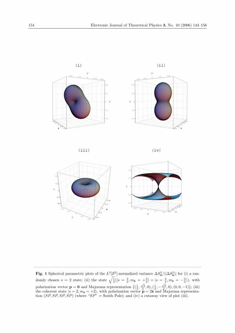
154 Electronic Journal of Theoretical Physics 3, No. 10 (2006) 143–156
Fig. 1 Spherical parametric plots of the L2[S2]-normalized variance ΔS2n/||ΔS2
n|| for (i) a ran-
domly chosen s = 2 state; (ii) the state√
12 (|s = 3
2 ,mz = + 32 〉 + |s = 3
2 ,mz = − 32 〉), with
polarization vector p = 0 and Majorana representation {( 12 ,
√3
2 , 0), ( 12 ,−
√3
2 , 0), (0, 0,−1)}; (iii)the coherent state |s = 2,mz = +2〉, with polarization vector p = 2z and Majorana representa-tion (SP, SP, SP, SP ) (where “SP” = South Pole); and (iv) a cutaway view of plot (iii).
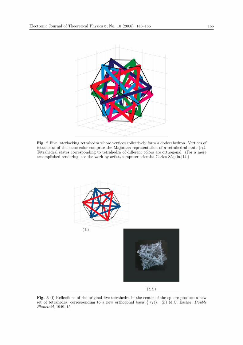
Electronic Journal of Theoretical Physics 3, No. 10 (2006) 143–156 155
Fig. 2 Five interlocking tetrahedra whose vertices collectively form a dodecahedron. Vertices oftetrahedra of the same color comprise the Majorana representation of a tetrahedral state |τk〉.Tetrahedral states corresponding to tetrahedra of different colors are orthogonal. (For a moreaccomplished rendering, see the work by artist/computer scientist Carlos Sequin.[14])
Fig. 3 (i) Reflections of the original five tetrahedra in the center of the sphere produce a newset of tetrahedra, corresponding to a new orthogonal basis {|τk〉}. (ii) M.C. Escher, DoublePlanetoid, 1949.[15]
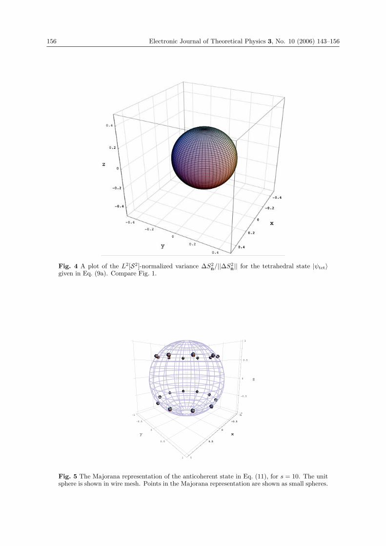
156 Electronic Journal of Theoretical Physics 3, No. 10 (2006) 143–156
Fig. 4 A plot of the L2[S2]-normalized variance ΔS2n/||ΔS2
n|| for the tetrahedral state |ψtet〉given in Eq. (9a). Compare Fig. 1.
-1
-0.5
0
0.5
1
x
-1
-0.5
0
0.5
1
y
-1
-0.5
0
0.5
1
z
-1
-0.5
0
0.5
1
x
Fig. 5 The Majorana representation of the anticoherent state in Eq. (11), for s = 10. The unitsphere is shown in wire mesh. Points in the Majorana representation are shown as small spheres.
EJTP 3, No. 10 (2006) 157–190 Electronic Journal of Theoretical Physics
Stretching the Electron as Far as it Will Go
Gordon W. Semenoff1 ∗ and Pasquale Sodano 2 †
1Department of Physics and AstronomyUniversity of British Columbia, Vancouver, British Columbia, Canada V6T 1Z1
2Progetto Lagrange, Fondazione C.R.T. e Fondazione I.S.I.c/o Dipartimento di Fisica- Politecnico di Torino,
Corso Duca degli Abruzzi 24 Torino-Italy
Received 8 May 2006, Published 28 May 2006
Abstract: Effects associated with the existence of isolated zero modes of Majorana fermionsare discussed. It is argued that the quantization of this system necessarily contains highlyextended quantum states and that populating and depopulating such states by interacting withthe quantum system leads to long-ranged teleportation-like processes. Also leads to spontaneousviolation of fermion parity symmetry. A quasi-realistic model consisting of a quantum wireembedded in a p-wave superconductor is discussed as an explicit example of a physical systemwith an isolated Majorana zero mode.c© Electronic Journal of Theoretical Physics. All rights reserved.
Keywords: Majorana Fermions, Teleportation, quantum Wire P-Wave superconductor, SolitonPACS (2006): 71.10.Pm, 05.30.Fk, 05.45.Yv, 78.67.Lt,85.35.Be, 74.20.-z
1. Introduction
It is a great pleasure to dedicate this article to the 100’th anniversary of the birth
of Ettore Majorana. As a testimony to his lasting influence on science, we shall describe
how one of his great insights, used in a modern context, can be related to a particular
macroscopic quantum phenomenon.
The idea is related to the observation by Majorana that a relativistic fermion such
as the electron can be meaningfully decomposed into more basic degrees of freedom,
essentially by taking the real and imaginary parts of its wave-function [1]. In relativistic
field theory, what one obtains are called Majorana fermions, which have become the
basic building blocks of supersymmetric field theories and supply a scenario whereby the
∗ This work is supported in part by NSERC of Canada.† Dipartimento di Fisica e Sezione INFN, Universit degli Studi di Perugia, Via A. Pascoli, 06123, Perugia
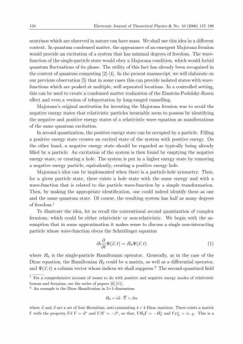
158 Electronic Journal of Theoretical Physics 3, No. 10 (2006) 157–190
neutrinos which are observed in nature can have mass. We shall use this idea in a different
context. In quantum condensed matter, the appearance of an emergent Majorana fermion
would provide an excitation of a system that has minimal degrees of freedom. The wave-
function of the single-particle state would obey a Majorana condition, which would forbid
quantum fluctuations of its phase. The utility of this fact has already been recognized in
the context of quantum computing [2]-[4]. In the present manuscript, we will elaborate on
our previous observation [5] that in some cases this can provide isolated states with wave-
functions which are peaked at multiple, well separated locations. In a controlled setting,
this can be used to create a condensed matter realization of the Einstein-Podolsky-Rosen
effect and even a version of teleportation by long-ranged tunnelling.
Majorana’s original motivation for inventing the Majorana fermion was to avoid the
negative energy states that relativistic particles invariably seem to possess by identifying
the negative and positive energy states of a relativistic wave equation as manifestations
of the same quantum excitation.
In second quantization, the positive energy state can be occupied by a particle. Filling
a positive energy state creates an excited state of the system with positive energy. On
the other hand, a negative energy state should be regarded as typically being already
filled by a particle. An excitation of the system is then found by emptying the negative
energy state, or creating a hole. The system is put in a higher energy state by removing
a negative energy particle, equivalently, creating a positive energy hole.
Majorana’s idea can be implemented when there is a particle-hole symmetry. Then,
for a given particle state, there exists a hole state with the same energy and with a
wave-function that is related to the particle wave-function by a simple transformation.
Then, by making the appropriate identification, one could indeed identify these as one
and the same quantum state. Of course, the resulting system has half as many degrees
of freedom.1
To illustrate the idea, let us recall the conventional second quantization of complex
fermions, which could be either relativistic or non-relativistic. We begin with the as-
sumption that in some approximation it makes sense to discuss a single non-interacting
particle whose wave-function obeys the Schrodinger equation
i�∂
∂tΨ(�x, t) = H0Ψ(�x, t) (1)
where H0 is the single-particle Hamiltonian operator. Generally, as in the case of the
Dirac equation, the Hamiltonian H0 could be a matrix, as well as a differential operator,
and Ψ(�x, t) a column vector whose indices we shall suppress.2 The second-quantized field
1 For a comprehensive account of issues to do with positive and negative energy modes of relativisticbosons and fermions, see the series of papers [6]-[11].2 An example is the Dirac Hamiltonian in 3+1-dimensions
H0 = i�α · �∇+ βm
where �α and β are a set of four Hermitian, anti-commuting 4× 4 Dirac matrices. There exists a matrixΓ with the property Γ�α Γ = �α∗ and ΓβΓ = −β∗, so that, ΓH0Γ = −H∗
0 and Γψ∗E = ψ−E . This is a
Electronic Journal of Theoretical Physics 3, No. 10 (2006) 157–190 159
operator also typically obeys this wave equation plus the equal-time anti-commutation
relation {Ψ(�x, t), Ψ†(�y, t)
}= δ(�x− �y) (2)
It is this anti-commutator which defines Ψ(x, t) as an operator. It can further be used to
derive the wave equation (1) from the second quantized Hamiltonian,
H =
∫dx : Ψ†(x, t)H0Ψ(x, t) : (3)
using the Hamilton equation of motion
i�∂
∂tΨ(x, t) = [Ψ(x, t), H]
We shall assume that H0 is a Hermitian operator which has eigenfunctions and a
spectrum of real eigenvalues
H0ψE(x) = EψE(x)
The energy E can be both positive and negative, in fact for the relativistic electron, if (1)
were the Dirac equation, there are necessarily negative eigenvalues and the spectrum is
unbounded below. The eigenfunctions obey the orthogonality and completeness relations∫d�xψ†
E(�x)ψE′(�x) = δEE′ ,∑
E
ψE(�x)ψ†E(�y) = δ(�x− �y) (4)
The delta function and summation in these formulae should be understood in a gener-
alized sense where they are a Kronecker delta and a sum for discrete components of the
spectrum and a Dirac delta function and integral for continuum spectrum.
In this system, one then forms the second quantized field operator by superposing the
wave-functions with creation and annihilation operators,
Ψ(x, t) =∑E>0
ψE(x)e−iEt/�aE +∑E<0
ψE(x)e−iEt/�b†−E
Here, aE is the annihilation operator for a particle with energy E and b†−E is the creation
operator for a hole with energy −E. When they obey the algebra with non-vanishing
anti-commutators {aE, a†
E′
}= δEE′ ,
{b−E, b†−E′
}= δEE′
the Ψ(�x, t) obeys the anticommutator (2). The completeness condition in Eq. (4) is
essential for establishing this.
one-to-one mapping of positive to negative energy states. Explicitly, if the matrices are represented by
�α =
⎛⎜⎝�σ 0
0 −�σ
⎞⎟⎠ with �σ the Pauli matrices and β =
⎛⎜⎝0 1
1 0
⎞⎟⎠, then we can form the matrix Γ =
⎛⎜⎝ 0 −iσ2
iσ2 0
⎞⎟⎠.
Note that, in this case Γ = Γ∗ and Γ2 = 1. A Majorana fermion obeys the reality condition Ψ(�x, t) =ΓΨ∗(�x, t).
160 Electronic Journal of Theoretical Physics 3, No. 10 (2006) 157–190
The ground state of the system, |0 >, is the state where all positive energy levels are
empty and where all negative energy levels are filled, or alternatively all hole states are
empty. In the second quantized language, it is annihilated by the annihilation operators,
aE|0 >= 0 = b−E|0 >
Excited states are created by operating on |0 > with a†E and b†−E. The excitations created
by a†E are particles, those created by b†−E are anti-particles, or holes. A typical state is
a†E1
. . . a†Em
b†E1. . . b†En
|0 >
and such states form a basis for the Fock space of the second quantized theory.
One can formulate Majorana fermions for a system of this kind if there exists a
particle-hole symmetry, or, in the relativistic context, a charge conjugation symmetry.
For example, consider the situation where a matrix Γ exists such that, for eigenstates of
H0,
ψ−E(x) = Γψ∗E(x) (5)
(This implies that Γ∗Γ = 1 = ΓΓ∗.) Then, the particles and holes have identical spectra.
A Majorana fermion is formed by treating the particle and hole with the same energy as
a single excitation. The second quantized field operator is
Φ(x, t) =∑E>0
(ψE(x)e−iEt/�aE + Γψ∗
E(x)eiEt/�a†E
)This fermion does not have both particles and anti-particles. The ground state |0 > is
annihilated by aE
aE|0 >= 0 ∀aE
and a†E creates particles, so that the excited states of the system are
a†E1
a†E2
...a†Ek|0 >
The field operator is (pseudo-)real in the sense that it obeys
Φ(x, t) = ΓΦ∗(x, t) (6)
It obeys the anti-commutation relation{Φ(�x, t), Φ†(�y, t)
}= δ(�x− �y) (7)
To be concrete, in a system of complex fermions where the Hamiltonian such that the
spectrum has the particle-hole symmetry (5), we could decompose the complex fermion
into two Majorana fermions by taking the real and imaginary parts,
Φ1(x, t) =1√2
(Ψ(x, t) + ΓΨ∗(x, t))
Electronic Journal of Theoretical Physics 3, No. 10 (2006) 157–190 161
Φ2(x, t) =1√2i
(Ψ(x, t)− ΓΨ∗(x, t))
Then each of Φ1(x, t) and Φ2(x, t) are a Majorana fermion.
In spite of the beautiful simplicity of this idea, Majorana fermions are not easy to come
by in nature. One could, for example, decompose the relativistic electron, whose wave
equation does have a charge-conjugation symmetry, into its real and imaginary parts.
However, the interaction of the electron with photons is not diagonal in this decomposi-
tion. The real and imaginary components would be rapidly re-mixed by electromagnetic
interactions, they cannot be stationary states of the full Hamiltonian of quantum elec-
trodynamics.
One place where we might have better luck is to look for emergent Majorana fermions
in quantum condensed matter systems. For example, in a superconductor, the electro-
magnetic interactions are effectively screened. Indeed, the Bogoliubov quasi-electrons in
a superconductor behave like neutral particles. However, even there, in an ordinary s-
wave superconductor, the anti-particle of a quasi-electron is another quasi-electron with
opposite spin. Indeed, the quasi-electron operator in an s-wave superconductor is the
two-component object ⎛⎜⎝ψ↑(x)
ψ∗↓(x)
⎞⎟⎠where (↑, ↓) denotes spin up and down. It obeys the charge conjugation condition⎛⎜⎝0 1
1 0
⎞⎟⎠⎛⎜⎝ψ↑(x)
ψ∗↓(x)
⎞⎟⎠∗
=
⎛⎜⎝ψ↓(x)
ψ∗↑(x)
⎞⎟⎠which is not an analog of the Majorana condition in eqn. (6), since it entails both conju-
gation and a flip of the spin.
In order to find a medium where the quasi-electron is a Majorana fermion, we need
to consider a superconductor where the condensate has Cooper pairs with the same spin,
so that the quasi-electron has the form⎛⎜⎝ψ↑(x)
ψ∗↑(x)
⎞⎟⎠Then, quasi-electron is pseudo-real, complex conjugation of its wave-function is equivalent
to multiplying by the matrix Γ =
⎛⎜⎝0 1
1 0
⎞⎟⎠,
⎛⎜⎝0 1
1 0
⎞⎟⎠⎛⎜⎝ψ↑(x)
ψ∗↓(x)
⎞⎟⎠∗
=
⎛⎜⎝ψ↑(x)
ψ∗↑(x)
⎞⎟⎠
162 Electronic Journal of Theoretical Physics 3, No. 10 (2006) 157–190
This gives a physical realization of a Majorana fermion. An example of such a super-
conductor is one with a p-wave condensate, such as Strontium Ruthenate [12]. There,
the condensate has the form 〈ψ↑(x)�x× �∇ψ↑(x)〉 (and can in principle have an admixture
of spin down as well). Thus, we see that, in such a material, the quasi-electron is a
two-component object obeying a Majorana condition. We will make use of this example
later in this Paper.
Our particular interest in the following will be in situations where the fermion spec-
trum has mid-gap, or zero energy states. These are well known to lead to interesting
phenomena. Already for complex electrons, mid-gap states give rise to fractional quan-
tum numbers [13, 14]. With Majorana fermions, they are known to lead to peculiar rep-
resentations of the anti-commutator algebra which can violate basic symmetries [15, 16].
Some interesting effects in the context of zero modes on cosmic strings have also been
examined [17]-[20].
To illustrate, let us consider the second quantization of a complex fermion whose
spectrum has a zero mode,
H0ψ0(x) = 0
The conjugation symmetry implies that
ψ0(x) = Γψ∗0(x)
If the fermion is complex (not Majorana), the second quantized field has a term with
the zero mode wave-function and an operator, the first term in the following expansion:
Ψ(x, t) = ψ0(x)α +∑E>0
ψE(x)e−iEt/�aE +∑E<0
ψE(x)e−iEt/�b†−E .
Here, α obeys the algebra {α, α†} = 1 (8)
and it anti-commutes with all of the other creation and annihilation operators. The
existence of this zero mode leads to a degeneracy of the fermion spectrum. The vacuum
state is annihilated by all of the annihilation operators aE and bE. However, it must also
carry a representation of the algebra (8). The minimal representation is two-dimensional.
There are two vacuum states, (| ↑>, | ↓>), which obey
aE| ↑>= 0 = aE| ↓> , bE| ↑>= 0 = bE| ↓>
and
α†| ↓>= | ↑> , α†| ↑>= 0
α| ↓>= 0 , α| ↑>= | ↓>The entire spectrum has a 2-fold degeneracy, with two towers of excited states,
a†E1
...a†Em
b†E1...b†En
| ↑>
Electronic Journal of Theoretical Physics 3, No. 10 (2006) 157–190 163
and
a†E1
...a†Em
b†E1...b†En
| ↓>having the identical energies
∑i Ei.
This quantization of the zero mode α was argued by Jackiw and Rebbi [13] to lead
to states with fractional fermion number. Indeed, the suitably normal ordered second
quantized number operator
Q =
∫d�x
1
2
[ψ†(x, t), ψ(�x, t)
]=∑E>0
(a†
EaE − b†−Eb−E
)+ α†α− 1
2(9)
has fractional eigenvalues, for example
Q| ↑>= +1
2| ↑> , Q| ↓>= −1
2| ↓>
In actuality, the charge operator is defined only up to an overall additive constant. How-
ever, there does exist a symmetry of the theory, gotten at the second quantized level
by replacing Ψ(x, t) by ΓΨ∗(x, t). This transformation interchanges particles and anti-
particles, and is a symmetry of the suitably normal ordered second quantized Hamilto-
nian. It should also flip the sign of Q. It implies that, if there is an eigenstate of Q in
the system with eigenvalue q,
Q|q >= q|q >
then there must exist another eigenstate | − q > in the spectrum of Q with eigenvalue
−q:
Q| − q >= −q| − q >
In addition, it is easy to argue that the eigenvalues of Q are space by integers, i.e. if
q1 and q2 are any two eigenvalues, then q1 − q2 =integer. This is essentially because the
raising and lowering operators for Q are Ψ† and Ψ, respectively and they raise and lower
in units of integers. In particular, this implies that
q − (−q) = 2q = integer
Thus, the only possibilities are that the entire spectrum of states have integer eigen-
values of Q, q =integer, or the entire spectrum of states have half-odd-integer eigenvalues
q = 12-odd integer. It is easy to see that the operator Q as written in (9) indeed flips
sign if we interchange aE ↔ bE and α↔ α† and the offset of -1/2 that appears explicitly
there is essential for this transformation to work. This leads to the conclusion that, with
a single fermion zero mode, the fermion number charge is quantized in half-odd-integer
units.
Now, consider what happens for a Majorana fermion with a single zero mode. 3 In
this case, a charge analogous to Q is not defined, so the issue of fractional charge is not
3 We will later construct an explicit example where this precisely this situation occurs.
164 Electronic Journal of Theoretical Physics 3, No. 10 (2006) 157–190
relevant. But the quantization of the system is still interesting. The second quantized
operator is
Φ(x, t) = ψ0(x)α +∑E>0
ψE(x)e−iEt/�aE +∑E<0
ψE(x)e−iEt/�a†−E
This fermion contains half of the degrees of freedom of the previous complex one. Here,
the bE are absent and the zero mode operator is real, α = α†.The creation and annihilation operator algebra is now{
aE, a†E′
}= δEE′
as before, and
α2 = 1/2 , {α, aE} = 0 ={
α, a†E
}(10)
A minimal representation can be constructed by defining a vacuum state where
aE|0 >= 0 for all E > 0
Then, we can represent the zero mode by the operator
α =1√2(−1)
�E>0 a†
EaE (11)
Indeed
α = α†
and, since ∑E
a†EaE|0 >= 0
we have
α|0 >=1√2|0 >
The Klein operator, (−1)�
E>0 a†EaE , anti-commutes with aE and a†
E. A basis for the
Hilbert space consists of the vacuum and excited states which are obtained from the
vacuum by operating creation operators
a†E1
a†E2
...a†Ek|0 >
These are eigenstates of∑
E>0 a†EaE with integer eigenvalues. Thus, in this basis, α2 =
1/2 when operating on each basis vector, and thus the identity operator on the whole
space. The operator in (11) thus satisfies the algebra (10).
Another, inequivalent representation can be obtained by starting with
α = − 1√2(−1)
�E>0 a†
EaE (12)
and a similar construction leads to a Hilbert space whose states are orthogonal the one
found above. We emphasize here that there are two inequivalent representations of the
Electronic Journal of Theoretical Physics 3, No. 10 (2006) 157–190 165
anti-commutator algebra, one where the zero mode operator is represented by α in eq. (11)
and one where it is represented by α in eq. (12). Both of these give an irreducible
representation and the two representations are not related to each other by an internal
automorphism.
We observe that these minimal representations of the anti-commutator algebra have
the property that they break a symmetry of the fermion theory under Φ(�x, t)→ −Φ(�x, t),
which we shall call “fermion parity”. Fermion parity is a symmetry of the linear wave
equation even when Φ(�x, t) is a Majorana fermion. At the quantum level, fermion parity
symmetry leads to a conservation law for the number of fermions modulo 2. By this con-
servation law, any physical process must entail creation or destruction of an even number
of fermions. For example, if a quantum state is initially prepared with an even number
of fermions, after any physical process, the number should remain even. In operator
language, there should exist an operator (−1)F which anti-commutes with Φ(�x, t),
(−1)F Φ(�x, t) + Φ(�x, t)(−1)F = 0
and which therefore commutes with the full second quantized Hamiltonian,
(−1)F H = H(−1)F
where
H =
∫d�x
1
2: Φ†(�x, t)H0Φ(�x, t) :
However, we see that in the minimal representations of the anti-commutation algebras
(10) discussed above, in the first representation (11),
< 0|Φ(x, t)|0 >= +1√2ψ0(x)
and in the second representation (12)
< 0|Φ(x, t)|0 >= − 1√2ψ0(x)
In both of these representations, neither the vacuum state, nor any of the excited states
can be eigenstates of fermion parity, the operator (−1)F . Thus fermion parity symmetry
is broken by the minimal quantization of this model.
Fermion parity is a sacred symmetry of physics in four dimensional space-time [21].
All fundamental fermions in nature have half-odd-integer spin. A flip in sign of all fermion
operators can then be realized as a rotation by an angle 2π. Nature should be symmetric
under a rotation by 2π. This means that, if we superpose a state with even fermion
number and a state with odd fermion number,
c1|even > +c2|odd >
no experiment should be devisable, even in principle, to measure the relative sign of c1
and c2. In the four dimensional world, unless rotation invariance is broken at a the level
166 Electronic Journal of Theoretical Physics 3, No. 10 (2006) 157–190
of fundamental physics, we should always be free to insist that (−1)F is a good symmetry
and that we can take all physical states as eigenstates. Of course, this applies in four
space-time dimensions. The emergent Majorana fermions that we want to consider here
are embedded in four space-time dimensions. We therefore feel free to insist on fermion
parity.
This brings up a contradiction with the previous discussion, where we found that
fermion parity is necessarily broken by the quantization of the zero mode Majorana
fermion system. The only way to restore the symmetry is to use a reducible represen-
tation of the anti-commutator algebra. The minimal modification of the representation
is equivalent to the introduction of another degree of freedom – and subsequent use of
irreducible representations. The new degree of freedom acts like a hidden variable. In
the anti-commutator algebra it would be another anti-commuting variable β which has
identical properties to α,
β2 = 1/2
and anti-commutes with all other variables. Then the algebra of α and β would have a two
dimensional representation which we could find by considering the fermionic oscillators
a =1√2
(α + iβ) , a† =1√2
(α− iβ) (13)
α =1√2
(a + a†) , β =
1√2i
(a− a†) (14)
which obey
a2 = 0 , a†2 = 0 ,{a, a†} = 1
We could then find a vacuum state which is annihilated by a, and another state which is
created from the vacuum by a†,
a|− >= 0 , a†|− >= |+ >
a|+ >= |− > , a†|+ >= 0
so that both are eigenstates of (−1)F and fermion parity is restored. Later we will see
that the hidden variable β can have a physical interpretation.
2. Degeneracy, Tunnelling and Teleportation
In this paper, the most speculative use of Majorana fermions that we shall find is
for a kind of teleportation by quantum tunnelling. In the context in which quantum
tunnelling is normally studied, a classical object can exist in allowed regions. There exist
other forbidden regions where it is not allowed to be. Then, quantum tunnelling makes
use of the fact that, when the particle is quantum mechanical, its wave-function does not
necessarily go to zero in a classically forbidden region, but decays exponentially. That
means that it could, in principle, have support on the other side of such a region and
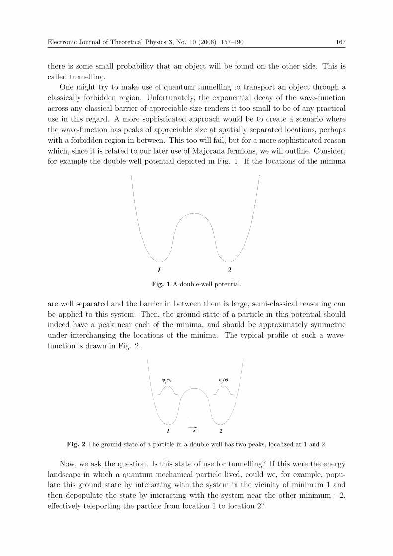
Electronic Journal of Theoretical Physics 3, No. 10 (2006) 157–190 167
there is some small probability that an object will be found on the other side. This is
called tunnelling.
One might try to make use of quantum tunnelling to transport an object through a
classically forbidden region. Unfortunately, the exponential decay of the wave-function
across any classical barrier of appreciable size renders it too small to be of any practical
use in this regard. A more sophisticated approach would be to create a scenario where
the wave-function has peaks of appreciable size at spatially separated locations, perhaps
with a forbidden region in between. This too will fail, but for a more sophisticated reason
which, since it is related to our later use of Majorana fermions, we will outline. Consider,
for example the double well potential depicted in Fig. 1. If the locations of the minima
21
Fig. 1 A double-well potential.
are well separated and the barrier in between them is large, semi-classical reasoning can
be applied to this system. Then, the ground state of a particle in this potential should
indeed have a peak near each of the minima, and should be approximately symmetric
under interchanging the locations of the minima. The typical profile of such a wave-
function is drawn in Fig. 2.
(x)ψ2
ψ1(x)
21 x
Fig. 2 The ground state of a particle in a double well has two peaks, localized at 1 and 2.
Now, we ask the question. Is this state of use for tunnelling? If this were the energy
landscape in which a quantum mechanical particle lived, could we, for example, popu-
late this ground state by interacting with the system in the vicinity of minimum 1 and
then depopulate the state by interacting with the system near the other minimum - 2,
effectively teleporting the particle from location 1 to location 2?
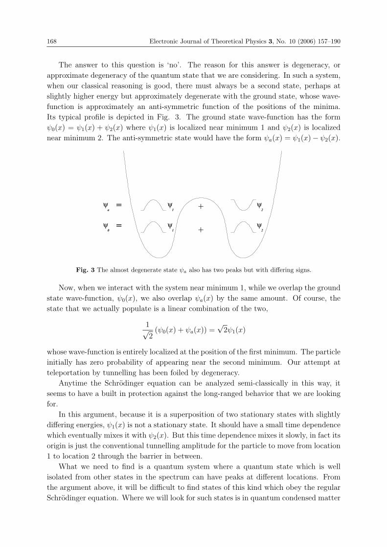
168 Electronic Journal of Theoretical Physics 3, No. 10 (2006) 157–190
The answer to this question is ‘no’. The reason for this answer is degeneracy, or
approximate degeneracy of the quantum state that we are considering. In such a system,
when our classical reasoning is good, there must always be a second state, perhaps at
slightly higher energy but approximately degenerate with the ground state, whose wave-
function is approximately an anti-symmetric function of the positions of the minima.
Its typical profile is depicted in Fig. 3. The ground state wave-function has the form
ψ0(x) = ψ1(x) + ψ2(x) where ψ1(x) is localized near minimum 1 and ψ2(x) is localized
near minimum 2. The anti-symmetric state would have the form ψa(x) = ψ1(x)− ψ2(x).
ψ2
ψ2
ψ1
ψ1
ψ0 +
+=
=
ψa
Fig. 3 The almost degenerate state ψa also has two peaks but with differing signs.
Now, when we interact with the system near minimum 1, while we overlap the ground
state wave-function, ψ0(x), we also overlap ψa(x) by the same amount. Of course, the
state that we actually populate is a linear combination of the two,
1√2
(ψ0(x) + ψa(x)) =√
2ψ1(x)
whose wave-function is entirely localized at the position of the first minimum. The particle
initially has zero probability of appearing near the second minimum. Our attempt at
teleportation by tunnelling has been foiled by degeneracy.
Anytime the Schrodinger equation can be analyzed semi-classically in this way, it
seems to have a built in protection against the long-ranged behavior that we are looking
for.
In this argument, because it is a superposition of two stationary states with slightly
differing energies, ψ1(x) is not a stationary state. It should have a small time dependence
which eventually mixes it with ψ2(x). But this time dependence mixes it slowly, in fact its
origin is just the conventional tunnelling amplitude for the particle to move from location
1 to location 2 through the barrier in between.
What we need to find is a quantum system where a quantum state which is well
isolated from other states in the spectrum can have peaks at different locations. From
the argument above, it will be difficult to find states of this kind which obey the regular
Schrodinger equation. Where we will look for such states is in quantum condensed matter
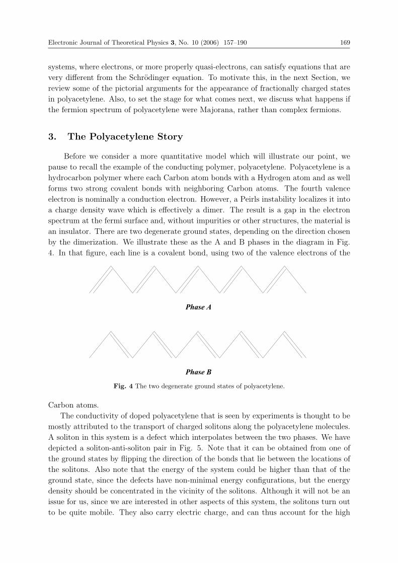
Electronic Journal of Theoretical Physics 3, No. 10 (2006) 157–190 169
systems, where electrons, or more properly quasi-electrons, can satisfy equations that are
very different from the Schrodinger equation. To motivate this, in the next Section, we
review some of the pictorial arguments for the appearance of fractionally charged states
in polyacetylene. Also, to set the stage for what comes next, we discuss what happens if
the fermion spectrum of polyacetylene were Majorana, rather than complex fermions.
3. The Polyacetylene Story
Before we consider a more quantitative model which will illustrate our point, we
pause to recall the example of the conducting polymer, polyacetylene. Polyacetylene is a
hydrocarbon polymer where each Carbon atom bonds with a Hydrogen atom and as well
forms two strong covalent bonds with neighboring Carbon atoms. The fourth valence
electron is nominally a conduction electron. However, a Peirls instability localizes it into
a charge density wave which is effectively a dimer. The result is a gap in the electron
spectrum at the fermi surface and, without impurities or other structures, the material is
an insulator. There are two degenerate ground states, depending on the direction chosen
by the dimerization. We illustrate these as the A and B phases in the diagram in Fig.
4. In that figure, each line is a covalent bond, using two of the valence electrons of the
Phase A
Phase B
Fig. 4 The two degenerate ground states of polyacetylene.
Carbon atoms.
The conductivity of doped polyacetylene that is seen by experiments is thought to be
mostly attributed to the transport of charged solitons along the polyacetylene molecules.
A soliton in this system is a defect which interpolates between the two phases. We have
depicted a soliton-anti-soliton pair in Fig. 5. Note that it can be obtained from one of
the ground states by flipping the direction of the bonds that lie between the locations of
the solitons. Also note that the energy of the system could be higher than that of the
ground state, since the defects have non-minimal energy configurations, but the energy
density should be concentrated in the vicinity of the solitons. Although it will not be an
issue for us, since we are interested in other aspects of this system, the solitons turn out
to be quite mobile. They also carry electric charge, and can thus account for the high
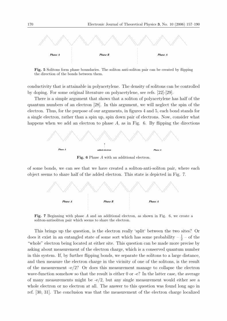
170 Electronic Journal of Theoretical Physics 3, No. 10 (2006) 157–190
Phase A Phase B Phase A
Fig. 5 Solitons form phase boundaries. The soliton anti-soliton pair can be created by flippingthe direction of the bonds between them.
conductivity that is attainable in polyacetylene. The density of solitons can be controlled
by doping. For some original literature on polyacetylene, see refs. [22]-[29].
There is a simple argument that shows that a soliton of polyacetylene has half of the
quantum numbers of an electron [28]. In this argument, we will neglect the spin of the
electron. Thus, for the purpose of our arguments, in figures 4 and 5, each bond stands for
a single electron, rather than a spin up, spin down pair of electrons. Now, consider what
happens when we add an electron to phase A, as in Fig. 6. By flipping the directions
Phase A Phase Aadded electron
Fig. 6 Phase A with an additional electron.
of some bonds, we can see that we have created a soliton-anti-soliton pair, where each
object seems to share half of the added electron. This state is depicted in Fig. 7.
Phase A Phase APhase B
Fig. 7 Beginning with phase A and an additional electron, as shown in Fig. 6, we create asoliton-antisoliton pair which seems to share the electron.
This brings up the question, is the electron really ‘split‘ between the two sites? Or
does it exist in an entangled state of some sort which has some probability – 12
– of the
“whole” electron being located at either site. This question can be made more precise by
asking about measurement of the electron charge, which is a conserved quantum number
in this system. If, by further flipping bonds, we separate the solitons to a large distance,
and then measure the electron charge in the vicinity of one of the solitons, is the result
of the measurement -e/2? Or does this measurement manage to collapse the electron
wave-function somehow so that the result is either 0 or -e? In the latter case, the average
of many measurements might be -e/2, but any single measurement would either see a
whole electron or no electron at all. The answer to this question was found long ago in
ref. [30, 31]. The conclusion was that the measurement of the electron charge localized
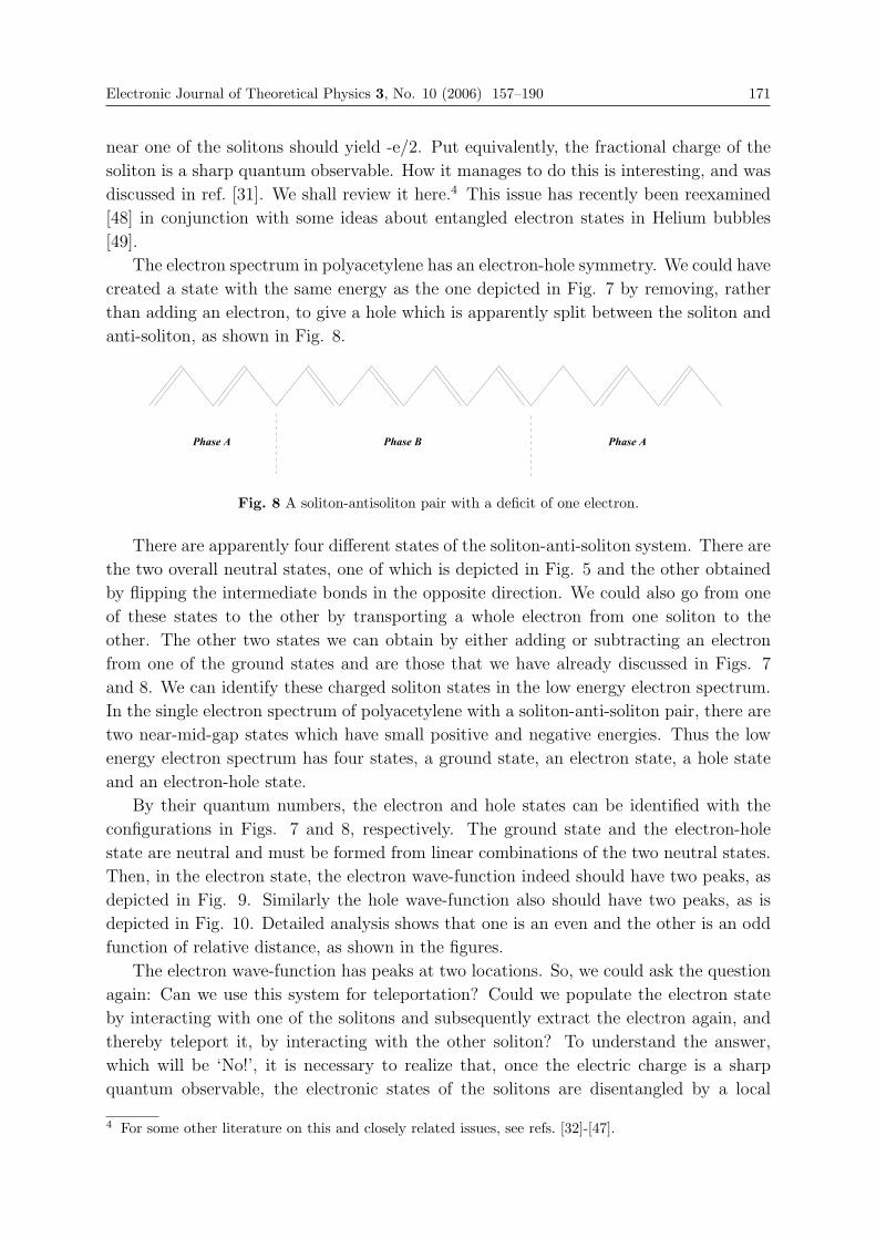
Electronic Journal of Theoretical Physics 3, No. 10 (2006) 157–190 171
near one of the solitons should yield -e/2. Put equivalently, the fractional charge of the
soliton is a sharp quantum observable. How it manages to do this is interesting, and was
discussed in ref. [31]. We shall review it here.4 This issue has recently been reexamined
[48] in conjunction with some ideas about entangled electron states in Helium bubbles
[49].
The electron spectrum in polyacetylene has an electron-hole symmetry. We could have
created a state with the same energy as the one depicted in Fig. 7 by removing, rather
than adding an electron, to give a hole which is apparently split between the soliton and
anti-soliton, as shown in Fig. 8.
Phase A Phase B Phase A
Fig. 8 A soliton-antisoliton pair with a deficit of one electron.
There are apparently four different states of the soliton-anti-soliton system. There are
the two overall neutral states, one of which is depicted in Fig. 5 and the other obtained
by flipping the intermediate bonds in the opposite direction. We could also go from one
of these states to the other by transporting a whole electron from one soliton to the
other. The other two states we can obtain by either adding or subtracting an electron
from one of the ground states and are those that we have already discussed in Figs. 7
and 8. We can identify these charged soliton states in the low energy electron spectrum.
In the single electron spectrum of polyacetylene with a soliton-anti-soliton pair, there are
two near-mid-gap states which have small positive and negative energies. Thus the low
energy electron spectrum has four states, a ground state, an electron state, a hole state
and an electron-hole state.
By their quantum numbers, the electron and hole states can be identified with the
configurations in Figs. 7 and 8, respectively. The ground state and the electron-hole
state are neutral and must be formed from linear combinations of the two neutral states.
Then, in the electron state, the electron wave-function indeed should have two peaks, as
depicted in Fig. 9. Similarly the hole wave-function also should have two peaks, as is
depicted in Fig. 10. Detailed analysis shows that one is an even and the other is an odd
function of relative distance, as shown in the figures.
The electron wave-function has peaks at two locations. So, we could ask the question
again: Can we use this system for teleportation? Could we populate the electron state
by interacting with one of the solitons and subsequently extract the electron again, and
thereby teleport it, by interacting with the other soliton? To understand the answer,
which will be ‘No!’, it is necessary to realize that, once the electric charge is a sharp
quantum observable, the electronic states of the solitons are disentangled by a local
4 For some other literature on this and closely related issues, see refs. [32]-[47].
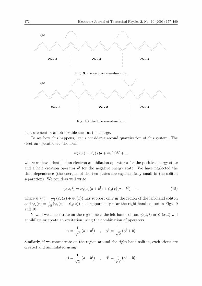
172 Electronic Journal of Theoretical Physics 3, No. 10 (2006) 157–190
ψe(x)
Phase APhase A Phase B
Fig. 9 The electron wave-function.
Phase A
(x)ψh
Phase A Phase B
Fig. 10 The hole wave-function.
measurement of an observable such as the charge.
To see how this happens, let us consider a second quantization of this system. The
electron operator has the form
ψ(x, t) = ψe(x)a + ψh(x)b† + ...
where we have identified an electron annihilation operator a for the positive energy state
and a hole creation operator b† for the negative energy state. We have neglected the
time dependence (the energies of the two states are exponentially small in the soliton
separation). We could as well write
ψ(x, t) = ψ1(x)(a + b†) + ψ2(x)(a− b†) + ... (15)
where ψ1(x) = 1√2(ψe(x) + ψh(x)) has support only in the region of the left-hand soliton
and ψ2(x) = 1√2(ψe(x)− ψh(x)) has support only near the right-hand soliton in Figs. 9
and 10.
Now, if we concentrate on the region near the left-hand soliton, ψ(x, t) or ψ†(x, t) will
annihilate or create an excitation using the combination of operators
α =1√2
(a + b†
), α† =
1√2
(a† + b
)Similarly, if we concentrate on the region around the right-hand soliton, excitations are
created and annihilated using
β =1√2
(a− b†
), β† =
1√2
(a† − b
)
Electronic Journal of Theoretical Physics 3, No. 10 (2006) 157–190 173
The set of operators (α, α†, β, β†) are a Bogoliubov transformation of the creation and
annihilation operators (a, a†, b, b†). This transformation does not violate fermion number
– it superposes operators with the same fermion number. Further, the excitations that
the new operators create or annihilate are entirely localized on one or the other of the
solitons.
Thus, again, we do not have a process whereby an electron or hole state which has
two peaks can be populated by interacting with the system in the vicinity of one of the
peaks. We have failed to find teleportation. Instead we have found fractional charge.
The charge density integrated over the vicinity of one of the solitons turns out to be
Q = −e(α†α− 1/2
)+ charge of electrons − charge of holes
which indeed has half-odd-integer eigenvalues. This Bogoliubov transformation, as a
mechanism for disentangling the charge quantum numbers of the solitons was originally
found in ref. [31].
In eq. (15), we ignored the small time dependence of the near mid-gap states. At
this point, the reader might wonder if the disentanglement of the soliton and anti-soliton
charges that we find by the Bogoliubov transformation would not be undone by this
time variation. Indeed, it would be, eventually. However the time scale is given by the
inverse of the energy gap and is therefore exponentially large in the distance L between
the soliton and anti-soliton, T ∼ m−1emL, where m is the energy gap. This is roughly
the time for quantum mechanical tunnelling between the solitons assuming an energy
barrier of height the energy gap extending over distance L. For macroscopic L this time
T should be very large.
What has prevented teleportation in this second example is again a degeneracy, this
time a slightly more subtle one since, even though the electron and hole state have
identical energies, they have opposite signs of charge. Avoiding teleportation has led to
fractional charge. It has done this by a hybridization, at the second quantized level, of
the propensity of the electron field operator to create an electron and to annihilate a hole
in a local state.
Now, imagine that, rather than complex electrons, polyacetylene had Majorana fermions
which would be obtained by identifying the particle and hole states as the same excita-
tions. (Here, we are ignoring the obvious disaster that this scenario would lead to in
chemistry.) Then, in eqn. (15), we would have to identify a = b and
ψMaj(x, t) = ψ1(x)(a + a†) + ψ2(x)(a− a†) + ... (16)
Now, a + a† cannot be an annihilation operator, in fact
(a + a†)2 = 1
It is similar to the single zero mode operator “α” that we found for a Majorana fermion
in the Eq. (14). In fact, the other combination 1√2i
(a− a†) now plays the role of “β”, the
“hidden variable”. Its purpose in our previous discussion was to provide a quantization
174 Electronic Journal of Theoretical Physics 3, No. 10 (2006) 157–190
which did not violate fermion parity. Here, this hidden variable is just the fermion zero
mode living on the far-away anti-soliton. We could choose the fermion parity conserving
quantization by using the states (|− >, |+ >) defined by
a|− >= 0 , a†|− >= |+ >
a|+ >= |− > , a†|+ >= 0
which can be eigenstates of (−1)F . In these states, the expectation value of the fermion
operator vanishes, for example < 0|ψMaj(x, t)|0 >= 0. However, the two solitons are
invariably entangled. There is now no conserved fermion number that we can use to
measure this entanglement, but there are other effects which we will discuss in later
sections once we have made the present reasoning more solid by discussing it in the
context of a field theoretical model and them formulated a more realistic model with
emergent Majorana fermions.
4. Relativistic Majorana Fermions in a Soliton Background
Single-particle states that are in some sense isolated are well known to occur for Dirac
equations, particularly when interacting with various topologically non-trivial background
fields such as solitons, monopoles and instantons. The consequences of fermion zero modes
such as chiral anomalies [50] and fractional fermion number [13], [14] are well known.
The polyacetylene example, in the context of discussions of fractional charge, that
we used in the previous Section is a well-known example of this. In polyacetylene, the
low energy electron spectrum can be approximately described by the Dirac equation [22,
51] and the solitons which we discussed using pictures have a mathematical description
as soliton-like configurations of a scalar field which couples to the Dirac equation. In
this Section, we will make the analysis of the previous Section more quantitative by
considering the problem of a 1+1-dimensional relativistic Dirac equation coupled to a
soliton background field and a soliton-anti-soliton pair.
Consider, for example, the simple one-dimensional model with Dirac equation
[iγμ∂μ + φ(x)] ψ(x, t) = 0 (17)
The Dirac gamma-matrices obey the algebra
{γμ, γμ} = 2gμν
where gμν =
⎛⎜⎝1 0
0 −1
⎞⎟⎠ is the (inverse of the) metric of two dimensional space-time.
This describes a fermion moving in one dimension and interacting with a scalar field
φ(x) which we shall take to have a soliton-anti-soliton profile. For the purposes of this
discussion, we take the ideal case of a step-function soliton located at position x = 0 and
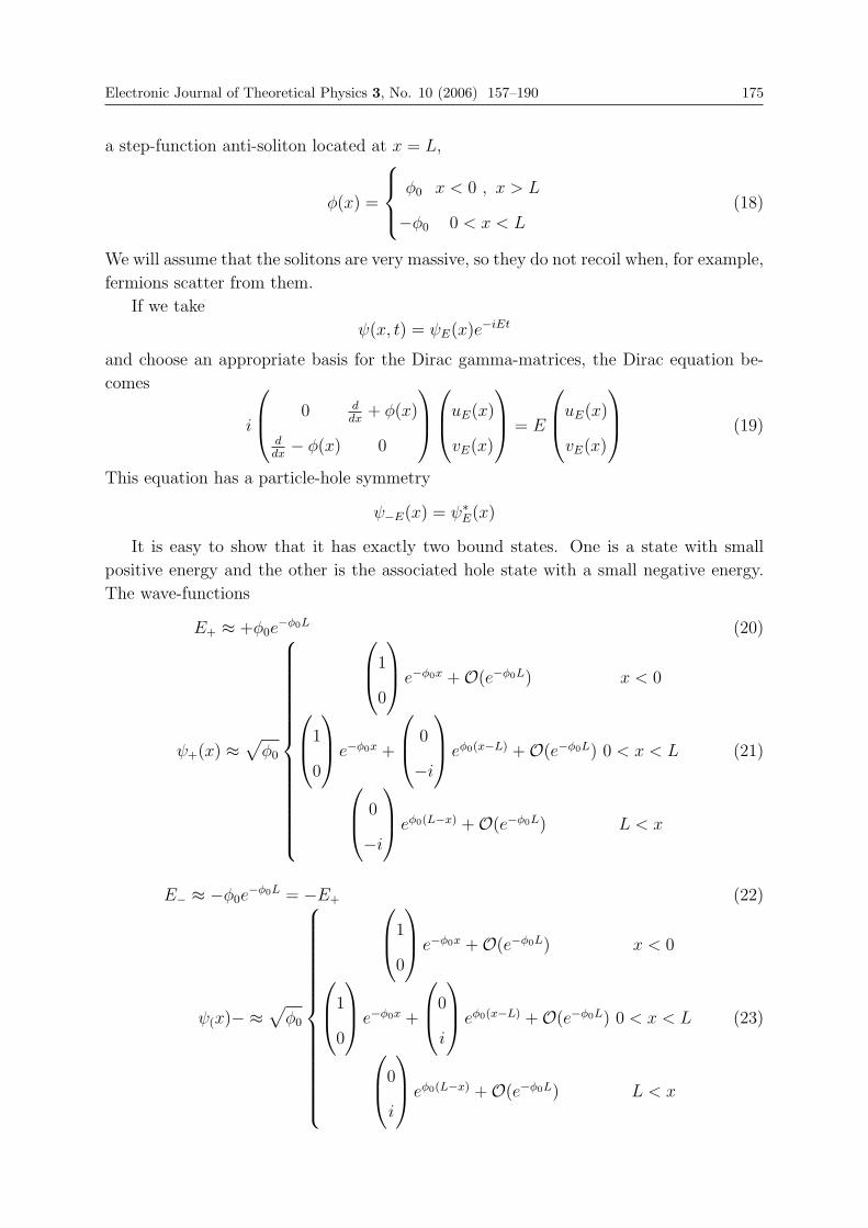
Electronic Journal of Theoretical Physics 3, No. 10 (2006) 157–190 175
a step-function anti-soliton located at x = L,
φ(x) =
⎧⎪⎨⎪⎩ φ0 x < 0 , x > L
−φ0 0 < x < L(18)
We will assume that the solitons are very massive, so they do not recoil when, for example,
fermions scatter from them.
If we take
ψ(x, t) = ψE(x)e−iEt
and choose an appropriate basis for the Dirac gamma-matrices, the Dirac equation be-
comes
i
⎛⎜⎝ 0 ddx
+ φ(x)
ddx− φ(x) 0
⎞⎟⎠⎛⎜⎝uE(x)
vE(x)
⎞⎟⎠ = E
⎛⎜⎝uE(x)
vE(x)
⎞⎟⎠ (19)
This equation has a particle-hole symmetry
ψ−E(x) = ψ∗E(x)
It is easy to show that it has exactly two bound states. One is a state with small
positive energy and the other is the associated hole state with a small negative energy.
The wave-functions
E+ ≈ +φ0e−φ0L (20)
ψ+(x) ≈√
φ0
⎧⎪⎪⎪⎪⎪⎪⎪⎪⎪⎪⎪⎪⎪⎪⎪⎨⎪⎪⎪⎪⎪⎪⎪⎪⎪⎪⎪⎪⎪⎪⎪⎩
⎛⎜⎝1
0
⎞⎟⎠ e−φ0x +O(e−φ0L) x < 0
⎛⎜⎝1
0
⎞⎟⎠ e−φ0x +
⎛⎜⎝ 0
−i
⎞⎟⎠ eφ0(x−L) +O(e−φ0L) 0 < x < L
⎛⎜⎝ 0
−i
⎞⎟⎠ eφ0(L−x) +O(e−φ0L) L < x
(21)
E− ≈ −φ0e−φ0L = −E+ (22)
ψ(x)− ≈√
φ0
⎧⎪⎪⎪⎪⎪⎪⎪⎪⎪⎪⎪⎪⎪⎪⎪⎨⎪⎪⎪⎪⎪⎪⎪⎪⎪⎪⎪⎪⎪⎪⎪⎩
⎛⎜⎝1
0
⎞⎟⎠ e−φ0x +O(e−φ0L) x < 0
⎛⎜⎝1
0
⎞⎟⎠ e−φ0x +
⎛⎜⎝0
i
⎞⎟⎠ eφ0(x−L) +O(e−φ0L) 0 < x < L
⎛⎜⎝0
i
⎞⎟⎠ eφ0(L−x) +O(e−φ0L) L < x
(23)
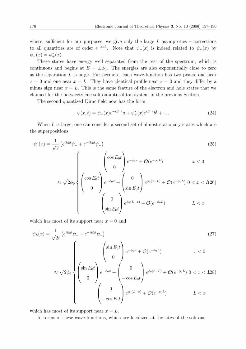
176 Electronic Journal of Theoretical Physics 3, No. 10 (2006) 157–190
where, sufficient for our purposes, we give only the large L asymptotics – corrections
to all quantities are of order e−φ0L. Note that ψ−(x) is indeed related to ψ+(x) by
ψ−(x) = ψ∗+(x).
These states have energy well separated from the rest of the spectrum, which is
continuous and begins at E = ±φ0. The energies are also exponentially close to zero
as the separation L is large. Furthermore, each wave-function has two peaks, one near
x = 0 and one near x = L. They have identical profile near x = 0 and they differ by a
minus sign near x = L. This is the same feature of the electron and hole states that we
claimed for the polyacetylene soliton-anti-soliton system in the previous Section.
The second quantized Dirac field now has the form
ψ(x, t) = ψ+(x)e−iE+ta + ψ∗+(x)eiE+tb† + . . . (24)
When L is large, one can consider a second set of almost stationary states which are
the superpositions
ψ0(x) =1√2
(eiE0tψ+ + e−iE0tψ−
)(25)
≈√
2φ0
⎧⎪⎪⎪⎪⎪⎪⎪⎪⎪⎪⎪⎪⎪⎪⎪⎨⎪⎪⎪⎪⎪⎪⎪⎪⎪⎪⎪⎪⎪⎪⎪⎩
⎛⎜⎝cos E0t
0
⎞⎟⎠ e−φ0x +O(e−φ0L) x < 0
⎛⎜⎝cos E0t
0
⎞⎟⎠ e−φ0x +
⎛⎜⎝ 0
sin E0t
⎞⎟⎠ eφ0(x−L) +O(e−φ0L) 0 < x < L
⎛⎜⎝ 0
sin E0t
⎞⎟⎠ eφ0(L−x) +O(e−φ0L) L < x
(26)
which has most of its support near x = 0 and
ψL(x) =1√2i
(eiE0tψ+ − e−iE0tψ−
)(27)
≈√
2φ0
⎧⎪⎪⎪⎪⎪⎪⎪⎪⎪⎪⎪⎪⎪⎪⎪⎨⎪⎪⎪⎪⎪⎪⎪⎪⎪⎪⎪⎪⎪⎪⎪⎩
⎛⎜⎝sin E0t
0
⎞⎟⎠ e−φ0x +O(e−φ0L) x < 0
⎛⎜⎝sin E0t
0
⎞⎟⎠ e−φ0x +
⎛⎜⎝ 0
− cos E0t
⎞⎟⎠ eφ0(x−L) +O(e−φ0L) 0 < x < L
⎛⎜⎝ 0
− cos E0t
⎞⎟⎠ eφ0(L−x) +O(e−φ0L) L < x
(28)
which has most of its support near x = L.
In terms of these wave-functions, which are localized at the sites of the solitons,
Electronic Journal of Theoretical Physics 3, No. 10 (2006) 157–190 177
ψ(x, t) = ψ0(x, t)1√2
(a + b†
)+ ψL(x, t)
1√2i
(−a + b†)
+ . . . (29)
We could now consider the creation and annihilation operators
α =1√2
(a + b†
), α† =
1√2
(a† + b
)β =
1√2i
(a† − b
), β† =
1√2i
(−a + b†)
By interacting with the system at x = 0, we could as well be dropping the fermion into
the state ψ0, which is localized there and which has exponentially vanishing probability
of occurring at x = L (until sin E0t becomes appreciable, which is just the usual estimate
of tunnelling time through a barrier of height φ0 and width L).
It might seem bizarre that, if we begin with the system in its ground state when
L is small, then adiabatically increase L that we would not simply end up with the
original ground state that has ψ−(x) populated, ψ+(x) empty. In fact, this is a possibility.
However, as we have argued in the polyacetylene example in the previous Section, as
L → ∞, the result is an entangled state of (appropriately defined [30, 31]) fermion
number. If we begin with the original ground state, measurement of the fermion number
which is localized in the vicinity of one of the solitons will collapse the wave-function
to one where the fermion, rather than occupying the negative energy state ψ−, occupies
either the state ψ0 or the state ψL which are localized at x = 0 or x = L, respectively. As
seen from the vicinity of each soliton, these are identical to the Jackiw-Rebbi states [13] of
the fermion in a single soliton background, which have fermion number ±12. These states
are time-dependent, but again, just as in the polyacetylene example, the time scale for
charge fluctuations is just the tunnelling time for a particle to go between the locations
of the solitons.
What about teleportation? Now, our dumping a fermion into the bound state, if
performed near x = 0 would populate the state ψ0(x), rather than ψ+(x), as all lo-
cal operators would couple only to this state. It would have appreciable probability of
appearing at x = L only after a time over order E−10 ∼ φ−1
0 eφ0L.
The situation is somewhat different if we assume that the fermion is a Majorana
fermion. The Hamiltonian of a Majorana fermion must have a symmetry which maps
positive energy states onto negative energy states. In the case of (19), we have ψ−E(x) =
ψ∗E(x). Then, a fermion and an anti-fermion have the same spectrum, and we can identify
them as the same particle.
Now, for the Majorana fermion, the pair of wave-functions ψ+(x) and ψ−(x) cor-
respond to the same quantum state which can be either occupied or empty. (We can
arbitrarily assign fermion parities (−1)F = −1 for the unoccupied state and (−1)F = 1
for the occupied state, although +i and −i might be more symmetric). In this case, the
states ψ0 and ψL are wave-functions for superpositions of the occupied and unoccupied
states – they do not have definite fermion parity.
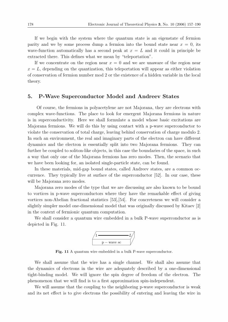
178 Electronic Journal of Theoretical Physics 3, No. 10 (2006) 157–190
If we begin with the system where the quantum state is an eigenstate of fermion
parity and we by some process dump a fermion into the bound state near x = 0, its
wave-function automatically has a second peak at x = L and it could in principle be
extracted there. This defines what we mean by “teleportation”.
If we concentrate on the region near x = 0 and we are unaware of the region near
x = L, depending on the quantization, this teleportation will appear as either violation
of conservation of fermion number mod 2 or the existence of a hidden variable in the local
theory.
5. P-Wave Superconductor Model and Andreev States
Of course, the fermions in polyacetylene are not Majorana, they are electrons with
complex wave-functions. The place to look for emergent Majorana fermions in nature
is in superconductivity. Here we shall formulate a model whose basic excitations are
Majorana fermions. We will do this by using contact with a p-wave superconductor to
violate the conservation of total charge, leaving behind conservation of charge modulo 2.
In such an environment, the real and imaginary parts of the electron can have different
dynamics and the electron is essentially split into two Majorana fermions. They can
further be coupled to soliton-like objects, in this case the boundaries of the space, in such
a way that only one of the Majorana fermions has zero modes. Then, the scenario that
we have been looking for, an isolated single-particle state, can be found.
In these materials, mid-gap bound states, called Andreev states, are a common oc-
currence. They typically live at surface of the superconductor [52]. In our case, these
will be Majorana zero modes.
Majorana zero modes of the type that we are discussing are also known to be bound
to vortices in p-wave superconductors where they have the remarkable effect of giving
vortices non-Abelian fractional statistics [53],[54]. For concreteness we will consider a
slightly simpler model one-dimensional model that was originally discussed by Kitaev [2]
in the context of fermionic quantum computation.
We shall consider a quantum wire embedded in a bulk P-wave superconductor as is
depicted in Fig. 11.
��
��
��
1 L
p− wave sc
Fig. 11 A quantum wire embedded in a bulk P-wave superconductor.
We shall assume that the wire has a single channel. We shall also assume that
the dynamics of electrons in the wire are adequately described by a one-dimensional
tight-binding model. We will ignore the spin degree of freedom of the electron. The
phenomenon that we will find is to a first approximation spin-independent.
We will assume that the coupling to the neighboring p-wave superconductor is weak
and its net effect is to give electrons the possibility of entering and leaving the wire in
Electronic Journal of Theoretical Physics 3, No. 10 (2006) 157–190 179
pairs by creating or destroying a p-wave cooper pair in the bulk. To describe the electrons,
we will use the Hamiltonian
H =L∑
n=1
(t
2a†
n+1an +t∗
2a†
nan+1 +Δ
2a†
n+1a†n +
Δ∗
2anan+1 + μa†
nan
)(30)
Sites on the quantum wire are labelled by n = 1, 2, ..., L. The operators an and a†n
annihilate and create an electron at site n. They obey the anti-commutator algebra{an, a
†n′
}= δnn′ (31)
The first terms in the Hamiltonian, with coefficients t and t∗ are the contribution
to the energy of the hopping of electrons between neighboring sites. The second pair
of terms, with Δ and Δ∗, arise from the presence of the super-conducting environment.
They describe the amplitude for a pair of electrons to leave or enter the wire from the
environment. It is assumed that they can do this as a Cooper pair when they are located
on neighboring sites. This is effectively an assumption about the size and coherence of
the cooper pairs in the superconductor. Even if it were not accurate, the smaller next-
to-nearest neighbor, etc. terms that would arise could be taken into account and would
not change our result significantly. The last term is the chemical potential, the energy
of an electron sitting on a site of the wire. We shall assume a reasonable hierarchy of
the parameters, that the amplitude for hopping along the wire is somewhat larger than
hopping to and from the bulk, |t| > |Δ|, and that the chemical potential is close enough
to zero that the electron band has substantial filling, |μ| < |t|.
5.1 Spectrum of Single-Particle States
Let us discuss the spectrum of the single-particle states in the many-body theory
described by the Hamiltonian (30). If t = |t|eiφ and Δ = |Δ|e2iθ, by redefining an →ei(φ+θ)an for n odd and an → ei(φ−θ)an for n even, we remove the complex phases of t and
Δ, which we can henceforth assume to be positive real numbers. The equation of motion
for the fermion wave-function is gotten by taking the commutator of its operator ak with
the Hamiltonian (30),
i�an = [an, H]
for which we get
i�d
dtan =
t
2(an+1 + an−1)− Δ
2
(a†
n+1 − a†n−1
)+ μan (32)
for the sites n = 2, ..., L− 1.
Because we are using open boundary conditions – the chain simply ends at n = 1 and
n = L, the equations for ddt
a1 and ddt
aL differ from (32) by missing terms. When we solve
(32) as a wave equation, it will be convenient to deal with this by extending the chain
180 Electronic Journal of Theoretical Physics 3, No. 10 (2006) 157–190
by one site in each direction and then eliminating the extra sites by imposing Dirichlet
boundary conditions,
a0(t) = 0 , aL+1(t) = 0
With these conditions, (32) describes the dynamics for all n = 1, 2, ..., L.
Now, it is most efficient to decompose the electron into real and imaginary parts,
an = bn + icn, and assemble them into a spinor
ψn =
⎛⎜⎝bn
cn
⎞⎟⎠ (33)
Note that this spinor obeys the Majorana condition
ψn = ψ∗n (34)
The equation for the wave-function is⎛⎜⎝ μ � ddt
−� ddt
μ
⎞⎟⎠ψn +
⎛⎜⎝12(t−Δ) 0
0 12(t + Δ)
⎞⎟⎠ψn+1 +
⎛⎜⎝12(t + Δ) 0
0 12(t−Δ)
⎞⎟⎠ψn−1 = 0 (35)
In order to solve the equation, we will make the ansatz
ψn(t) = e−iωt/�ψn(ω) (36)
The Majorana condition for energy eigenstates is
ψ∗n(ω) = ψn(−ω)
We will normalize the wave-functions with the condition
L∑n=1
|ψn(ω)|2 = 1 =L∑
n=1
(|bn(ω)|2 + |cn(ω)|2)Since the equation and boundary conditions are linear, we can further make the ansatz
that the wave-functions are superpositions of plane waves,
ψn(ω) = ζn
⎛⎜⎝u(ζ)
v(ζ)
⎞⎟⎠ (37)
Then, the difference equation (35) becomes
The equation for the wave-function is⎛⎜⎝12t(ζ + 1/ζ)− 1
2Δ(ζ − 1/ζ) + μ −iω
iω 12t(ζ + 1/ζ)− 1
2Δ(ζ − 1/ζ) + μ
⎞⎟⎠⎛⎜⎝u(ζ)
v(ζ)
⎞⎟⎠ = 0 (38)
Electronic Journal of Theoretical Physics 3, No. 10 (2006) 157–190 181
which has a solution when the frequencies obey the dispersion relation
ω2 =
[1
2t(ζ + 1/ζ) + μ
]2
−[1
2Δ(ζ − 1/ζ)
]2
(39)
For a given real value of ω, there are generally four wave-vectors which satisfy this dis-
persion relation,
ζω , 1/ζω , ζ∗ω , 1/ζ∗
ω
To find a solution of the wave equation, we must take superpositions of the four solutions
of (38) with each of these four wave-vectors. Then we must adjust the four coefficients
of the superposition in order to satisfy the four boundary conditions. (Remember that
the boundary conditions are for spinors, so there are four boundary conditions in total.)
Three of the boundary conditions can be solved by adjusting the coefficients in the super-
position. The fourth superposition coefficient can eventually be determined up to phases
by normalizing the wave-function. The fourth boundary condition, which has yet to be
satisfied, then gives a condition that the wave-vector must obey. Plugging the resulting
wave-vector back into the dispersion relation (39) then gives the allowed energy eigen-
value. This gives an algorithm for finding the energies, the allowed wave-vectors (which
are 1iln ζ and are generally complex) and the wave-functions.
When L is large, the solutions are of two kinds. One are to a good approximation
continuum states, where ζ = eik and the continuum spectrum is
ω(k) = ±√
[t cos k + μ]2 + Δ2 sin2 k
with k ∈ (−π, π] (it is quantized approximately as k = 2π · integer/(L+1) which becomes
a continuum when L → ∞). This spectrum has an energy gap. The point of closest
approach of the positive and negative energy bands occurs when cos k = −tμ/(t2 −Δ2)
and the gap is Egap = 2Δ√
t2−Δ2−μ2
t2−Δ2 . We will assume that this gap is significant, so that
the mid-gap states that we will discuss next are indeed well isolated.
The other modes in the spectrum are a pair of mid-gap states. When L is large, these
states have energies that are exponentially small in L, one is positive, one is negative
and they have equal magnitudes. In the following, we will solve for the spectrum of these
mid-gap states in the approximation where effects that are exponentially small in L are
neglected.
We begin with an un-normalized spinor
ζn
⎛⎜⎝ iω
12t(ζ + 1/ζ)− 1
2Δ(ζ − 1/ζ) + μ
⎞⎟⎠+ Aζ−n
⎛⎜⎝ iω
12t(ζ + 1/ζ) + 1
2Δ(ζ − 1/ζ) + μ
⎞⎟⎠+Bζ∗n
⎛⎜⎝ iω
12t(ζ∗ + 1/ζ∗)− 1
2Δ(ζ∗ − 1/ζ∗) + μ
⎞⎟⎠+ Cζ∗−n
⎛⎜⎝ iω
12t(ζ∗ + 1/ζ∗) + 1
2Δ(ζ∗ − 1/ζ∗) + μ
⎞⎟⎠(40)
182 Electronic Journal of Theoretical Physics 3, No. 10 (2006) 157–190
We will solve the boundary condition for the mid-gap state in the limit where L is
large. There, we expect the solution to be very close to ω = 0, for which we then
need a wave-vector which solves t(ζ + 1/ζ) + 2μ = −Δ(ζ − 1/ζ). Then, to a first
approximation, the terms with A and C are absent from (40) and we must choose the
B = −(ζ − 1/ζ)/(ζ∗ − 1/ζ∗) in order to satisfy the boundary condition at n = 0. Since
ζ = − μ
2(t + Δ)+ i
√t−Δ
t + Δ
√1− μ2/4(t2 −Δ2)
so that ζζ∗ = t−Δt+Δ
< 1, this gives a wave-function which is maximal at n = 1 and which
decays exponentially as n increases. This would indeed be the solution for the mid-gap
state on the half-line when L → ∞. When L is finite, rather than infinite, in order to
satisfy the boundary condition at n = L+1 we must include an amplitude for the growing
solution. It can be obtained from the decaying one by simply replacing n by L + 1 − n
and multiplying the spinor by σ2. Thus, to a good approximation the mid-gap solution
is
ψ+n =
√Δ
2t
t2 − μ2
t2 −Δ2 − μ2
⎡⎢⎣(−μ + i
√t2 −Δ2 − μ2
)n
−(−μ− i
√t2 −Δ2 − μ2
)n
(t + Δ)n
⎛⎜⎝0
i
⎞⎟⎠+
+
(−μ + i
√t2 −Δ2 − μ2
)L+1−n
−(−μ− i
√t2 −Δ2 − μ2
)L+1−n
(t + Δ)L+1−n
⎤⎥⎦⎛⎜⎝1
0
⎞⎟⎠This wave-function has infinitesimal positive energy. The wave-function with infinitesimal
negative energy is given by
ψ−n =
√Δ
2t
t2 − μ2
t2 −Δ2 − μ2
⎡⎢⎣(−μ + i
√t2 −Δ2 − μ2
)n
−(−μ− i
√t2 −Δ2 − μ2
)n
(t + Δ)n
⎛⎜⎝0
i
⎞⎟⎠−−(−μ + i
√t2 −Δ2 − μ2
)L+1−n
−(−μ− i
√t2 −Δ2 − μ2
)L+1−n
(t + Δ)L+1−n
⎤⎥⎦⎛⎜⎝1
0
⎞⎟⎠We will abbreviate these by naming the function
φn = i
√Δ
2t
t2 − μ2
t2 −Δ2 − μ2
(−μ + i
√t2 −Δ2 − μ2
)n
−(−μ− i
√t2 −Δ2 − μ2
)n
(t + Δ)n(41)
where φn = φ∗n and we have normalized to
∑n
|φn|2 =1
2(42)
Electronic Journal of Theoretical Physics 3, No. 10 (2006) 157–190 183
The function φn has maximum magnitude at n = 1 and it decays exponentially as n
increases. We shall use the notation
ψ+n = φn
⎛⎜⎝0
1
⎞⎟⎠− φL+1−n
⎛⎜⎝i
0
⎞⎟⎠ (43)
ψ−n = φn
⎛⎜⎝0
1
⎞⎟⎠+ φL+1−n
⎛⎜⎝i
0
⎞⎟⎠ (44)
We have normalized the spinors so that∑n
ψ±†n ψ±
n = 1 (45)
Note that, these wave-functions satisfy the Majorana condition ψ−n = ψ+∗
n . As ex-
pected, they have support near n = 1 and n = L and are exponentially small in the
interior of the quantum wire, far from the boundaries. Further, we have adjusted phases
so that the wave-functions are identical in profile in the region near n = 1. Then, we
expect that they differ in sign in the region near n = L and we confirm from that above
that this is so. Also, note that they are complex. To form the real, Majorana spinor, we
must superpose them with a creation and annihilation operator,
ψn(t) = ψ+n e−iωta + ψ−
n eiωta† + non− zero energy states (46)
Here a and a† are the annihilation and creation operators for the mid-gap state and ω is
their exponentially small energy. Ignoring the energy, we can also write this operator as
ψn(t) = φn
⎛⎜⎝0
1
⎞⎟⎠ (a + a†) + φL+1−n
⎛⎜⎝1
0
⎞⎟⎠ 1
i(a− a†) + . . .
The first term on the right-hand side has support near n = 0 and decays exponentially as
n increases from 1. The second term has support near n = L and decays exponentially
as n decreases from L. They each multiply the operators α = 1√2
((a + a†) and β =
1√2i
(a− a†), respectively. These are analogous to the operators which we introduced on
Section 1. a and a† must have the anti-commutator{a, a†} = 1
which has a two-dimensional representation, the states |− > and |+ > of Section 1 which
we copy here for the reader’s convenience,
a|− >= 0 , a†|− >= |+ >
a|+ >= |− > , a†|+ >= 0
All other excited states of the system are created by operating creation operators for the
other, non-zero energy excitations. Remember that it is the states |+ > and |− > which
we expect to be eigenstates of fermion parity, (−1)F .
184 Electronic Journal of Theoretical Physics 3, No. 10 (2006) 157–190
5.2 Second Quantized Electron Operator
Now, we recall that the upper and lower components of the spinor ψn(t) that we
discussed in the previous subsection are simply the real and imaginary components of the
electron field operator, which we can now reconstruct,
an(t) = φL+1−n1
i
(a− a†)+ iφn
(a + a†)+ . . . (47)
This is now a complex operator, but its real and imaginary parts have support at opposite
ends of the quantum wire. The part of the operator which has not been written, and is
indicated by dots in (47), are superpositions of creation and annihilation operators for
continuum states. All such states have energies above the gap and extended, plane-wave-
like wave-functions. Note that now that the phase symmetry of the system has been
broken by coupling to the superconductor, the real and imaginary parts of the electron
operator will generally have different properties. This interesting fact will not concern
us in the following and we will focus on the mid-gap, or zero mode part of the electron
operator.
Note, now, if we operate with any local operator in the vicinity of n = 1, the electon
operator acts as if it were composed of the combination of zero mode operators (a + a†).As we have discussed before, this operator squares to a constant. There cannot be any
states that it annihilates. Thus, operating it on any state of the system, in the region
where the zero mode wavefunction has support, will have an effect. What it does is flip
the state from |− > to |+ >. Since it is a hermitian operator, it is possible to diagonalize
it, the states 1√2(|− > +|+ >) and 1√
2(|− > +|+ >) are its eigenvectors. However, these
eigenvectors are not eigenstates of fermion parity.
6. Long Ranged Correlations of Electrons
What about teleportation? Let us imagine that we begin with the system in one
of its ground states, say |− > and inject an electron so that at time T = 0 it is resting
at site #1. This means, we being with the state a†1|− >, where, as we recall, a†
1 is the
creation operator for an electron at site #1.
We then ask what is the quantum transition amplitude for the transition, after a time
T has elapsed, of this state to one with the electron located at position #L. The final
quantum state is a†L|− >. The amplitude is given by
A =< −| aL eiHT a†1 |− >= |φ0
1|2 + (T and L−dependent) (48)
The T - and L-dependent parts of this matrix element represent the usual propagation via
excited quasi-electrons which must travel across the wire. The first term is non-zero and
is T and L-independent. By ‘teleportation’, we are referring to this part of the amplitude.
Here, we can evaluate the amplitude explicitly. It is
ATel =
(2Δ
t
)(t2 −Δ2 − μ2
(t + Δ)2
)(49)
Electronic Journal of Theoretical Physics 3, No. 10 (2006) 157–190 185
Which can be appreciable, in the 10-30 percent range, for a surprisingly wide choice of
parameters.
However, the teleportation probability is the square of this amplitude, which is some-
what smaller. We could ask a more sophisticated question: What is the probability that
the electron, once injected at n = 1 appears anywhere within the exponential range of
the zero mode wave-function at n = L. This probability would be given by
PTel =∑
n
|φn|2|φ01|2 =
1
2
(2Δ
t
)(t2 −Δ2 − μ2
(t + Δ)2
)(50)
This is what we shall call the “teleportation probability“. Again, for a range of parameters
t, Δ and μ, it can be appreciable.
7. Discussion
The apparently instantaneous propagation of an electron would seem to be a poten-
tial violation of Einstein causality, since in principle a message could be sent at a speed
faster than that of light.
Let us review the nature of the system that we have constructed. Once the quantum
wire - p-wave superconductor system is prepared, the extended Majorana state of the
electron is already there, ready for use. The system has a two-fold degeneracy: at low
energy, there are two states |− > and |+ >. These are not normal quantum states in
that they differ by a quantum number which we would like to preserve, fermion parity
(−1)F .
Thus, if we do not allow superpositions of these states, this is effectively a classical
bit, like a classical switch that can either be OFF or ON, the wave-function can be in
one state or the other.
The system moves from OFF to ON by absorbing or emitting an electron in a way
that flips the vacuum from one state to the other. This should occur somewhere in the
vicinity of the ends of the wire, where the zero mode wave-functions have support. It
can move back from ON to OFF by the identical process, again absorbing or emitting a
single electron.
This leads to the rather drastic conclusion that there could be super-luminal transfer
of information in this system. One would need only to prepare the system in one of its
ground states, with a sender sitting at 1 and a receiver sitting at L. Either ground state
is sufficient and neither the sender nor the observer needs to know which it is. All the
receiver has to do is wait for an electron to arrive. If it arrives with energy at or above
the electron energy gap, he or she can conclude that it propagated normally and was
sent at some time in the past. However, if it arrives at very low energy, he or she knows
that it tunnelled and that it was sent by the sender at that instant. This is seemingly an
instant transfer of information over a finite distance.
There is a obvious way out of this, but it means giving up the fermion parity sym-
metry that has until now been sacred. If we allow superpositions of the states |− > and
186 Electronic Journal of Theoretical Physics 3, No. 10 (2006) 157–190
|+ > which have even and odd fermion number, then the degenerate ground states are
a quantum rather than classical two-level system, there are two states and any superpo-
sitions are allowed. Now, in this system, it is easy to prepare states where an electron
can spontaneously appear or disappear. Take, for example an eigenstate of the operators
that we called α and β. In their eigenstates, 1√2(|− > ±|+ >), the electron operator has
an expectation value < an(t) >= ±φn ± φL+1−n. It would thus have an amplitude for
simply vanishing or appearing spontaneously.
Then, when the observer at L detects the arrival of a low energy electron he or she
cannot distinguish one which was sent from the other side of the wire from one which
is spontaneously created. This restores Einstein causality at the expense of our having
to admit states onto physics which are not eigenstates of fermion parity. There is the
further question of whether such states are consistent with three dimensional physics.
Fermion number mod 2 is an important conservation law in three dimensional physics [55].
Even though the quantum wire that we have discussed is one-dimensional, it is embedded
in three dimensional space and the electrons that we are discussing are spin-12
particles in
three dimensional space. This means that their wave-functions individually change sign
under a rotation by 2π. More importantly, a state with odd fermion number must change
sign under a rotation by 2π whereas a state with even number should remain unchanged.
A rotation by angle 2π should not affect physics. Thus, the relative sign of even and odd
fermion number states should not have any physical consequences.
If we did allow a superposition of the two states, they would form a single qubit. We
could parameterize the state-vector by a point on the Bloch sphere (θ, φ) where the state
is
|θ, ϕ > = cosθ
2|− > +eiϕ sin
θ
2|+ > (51)
Points on the two-dimensional unit sphere are specified by the unit vectors
n = (sin θ cos ϕ, sin θ sin ϕ, cos θ)
and 0 ≤ θ ≤ π, −π < ϕ ≤ π. However, as we have argued, the relative sign of the two
states should not be an observable. Then the set of “physical states” of the qubit would
be the Bloch sphere with a further identification
ϕ ∼ ϕ + π (52)
Of course, this identification is allowed only if there are no experiments, even in principle,
which could measure the relative sign of the two states in the superposition. Normally,
one could measure that sign by an interference experiment.
For example, we could attempt to observe the relative sign by examining interference
between the electron which arrives by tunnelling and the one which arrives by conventional
transport. However, the teleportation amplitude in the state φ
< θ, ϕ| aL eiHT a†1 |θ, ϕ >= cos θ[teleportation] + [transport] (53)
The teleportation amplitude is diminished by a factor of cos θ whereas the transport
amplitude is unchanged. One can make the teleportation amplitude vanish by adjusting
Electronic Journal of Theoretical Physics 3, No. 10 (2006) 157–190 187
θ = π/2. However, the relative amplitude cannot be used to measure the relative sign of
the two components of the wave-function.
There is an amplitude for an electron to vanish,
< θ, ϕ| eiHT a†1 |θ, ϕ >∼ i sin θ cos ϕ · φ1 (54)
and to appear spontaneously
< θ, ϕ| aL eiHT |θ, ϕ >∼ sin θ sin ϕ · φ1 (55)
As we expect, the latter two amplitudes change sign when we put ϕ → ϕ + π. Actual
quantum observables are probabilities which are the modulus squares of amplitudes. They
are also insensitive to the relative sign of the two parts of the wave-function.
The above probability amplitudes do not offer a way to distinguish the quantum
states with ϕ and ϕ + π. At this point, we have not ruled out, but also we have not
devised an experiment by which they could be distinguished. Indeed, if there is no such
experiment, we are free to cut the Bloch sphere in half by the identification (52) and the
ground states would form this peculiar qubit. Teleportation still happens, but so does
the spontaneous disappearance or appearance of a single electron and the contradiction
with Einstein locality is removed.
We cannot exclude the possibility that the effect that we have been discussing could
be interfered with by the superconductor which the quantum wire is in contact with.
Here, we have assumed that it acts as a simple bath which supplies and absorbs Cooper
pairs but is otherwise innocuous. We cannot rule out that it also has exotic states that
should be included in the picture.
Acknowledgements
G.S. thanks Duncan Haldane, Tony Leggett, Girard Milburn and Bill Unruh for dis-
cussions and acknowledges the hospitality of the I.H.E.S., Bures-sur-Yvette, the Werner
Heisenberg Institute, Munich and the University of Perugia where parts of this work
were completed. P.S. thanks M.Rasetti, P. Zanardi and V. Barone for discussions and
acknowledges the Pacific Institute for Theoretical Physics, Vancouver and the Center for
Theoretical Physics at MIT for hospitality. This work is supported in part by NSERC of
Canada and by M.I.U.R. National Project ”JOSNET” (grant n.2004027555).
188 Electronic Journal of Theoretical Physics 3, No. 10 (2006) 157–190
References
[1] E. Majorana, Nuovo Cimento, Vol.5, 171 (1937).
[2] Alexei Kitaev, ”Unpaired Majorana fermions in quantum wires” [arXiv:cond-mat/0010440]
[3] L. S. Levitov, T. P. Orlando, J. B. Majer and J. E. Mooij, “Quantum spin chainsand Majorana states in arrays of coupled qubits”, [arXiv:cond-mat/0108266]
[4] U. Dorner, P. Fedichev, D. Jaksch, K. Lewenstein and P. Zoller, “Entangling stringsof neutral atoms in 1D atomic pipeline structures” [arXiv.org:quant-ph/0212039]
[5] Gordon W. Semenoff and P. Sodano, ” Teleportation by a Majorana Medium”[arXiv:cond-mat/0601261].
[6] H. B. Nielsen and M. Ninomiya, “Dirac sea for bosons,” arXiv:hep-th/9808108.
[7] Y. Habara, H. B. Nielsen and M. Ninomiya, “Boson sea versus Dirac sea: Generalformulation of boson sea through Int. J. Mod. Phys. A 19, 5561 (2004) [arXiv:hep-th/0312302].
[8] H. B. Nielsen and M. Ninomiya, “Dirac sea for bosons. I: Formulation of negativeenergy sea for bosons,” Prog. Theor. Phys. 113, 603 (2005) [arXiv:hep-th/0410216].
[9] H. B. Nielsen and M. Ninomiya, “Dirac sea for bosons. II: Study of the naive vacuumtheory for the Prog. Theor. Phys. 113, 625 (2005) [arXiv:hep-th/0410218].
[10] Y. Habara, H. B. Nielsen and M. Ninomiya, “Negative energy (Dirac-like) sea forbosons and supersymmetry,” arXiv:hep-th/0501095.
[11] Y. Habara, H. B. Nielsen and M. Ninomiya, “Hole theory of boson sea,” arXiv:hep-th/0504173.
[12] Y.Maeno, T.M. Rice, M. Sigrist, Physics Today, 54, 42 (2001).
[13] R. Jackiw and C. Rebbi, “Solitons With Fermion Number 1/2,” Phys. Rev. D 13,3398 (1976).
[14] For a review, see A. J. Niemi and G. W. Semenoff, “Fermion Number FractionizationIn Quantum Field Theory,” Phys. Rept. 135, 99 (1986) and for material closelyrelated to the present paper, A. J. Niemi and G. W. Semenoff, “Spectral AsymmetryOn An Open Space,” Phys. Rev. D 30, 809 (1984).
[15] A. Losev, M. A. Shifman and A. I. Vainshtein, “Single state supermultiplet in 1+1dimensions,” New J. Phys. 4, 21 (2002) [arXiv:hep-th/0011027].
[16] A. Losev, M. A. Shifman and A. I. Vainshtein, “Counting supershortsupermultiplets,” Phys. Lett. B 522, 327 (2001) [arXiv:hep-th/0108153].
[17] G. D. Starkman, D. Stojkovic and T. Vachaspati, “Neutrino zero modes onelectroweak strings,” Phys. Rev. D 63, 085011 (2001) [arXiv:hep-ph/0007071].
[18] G. Starkman, D. Stojkovic and T. Vachaspati, “Zero modes of fermions with a generalmass matrix,” Phys. Rev. D 65, 065003 (2002) [arXiv:hep-th/0103039].
[19] D. Stojkovic, “Fermionic zero modes on domain walls,” Phys. Rev. D 63, 025010(2001) [arXiv:hep-ph/0007343].
[20] D. Stojkovic, “Neutrino zero modes and stability of electroweak strings,” Int. J. Mod.Phys. A 16S1C, 1034 (2001) [arXiv:hep-th/0103216].
Electronic Journal of Theoretical Physics 3, No. 10 (2006) 157–190 189
[21] R. F. Streater and A. S. Wightman, “Pct, Spin And Statistics, And All That,”Redwood City, USA: Addison-Wesley (1989) (Advanced book classics).
[22] W. P. Su, J. R. Schrieffer and A. J. Heeger, “Solitons In Polyacetylene,” Phys. Rev.Lett. 42 (1979) 1698.
[23] M. J. Rice, Phys. Lett. A71, 152 (1979.
[24] S. A. Brazovskii, JETP Lett. 28, 656 (1978).
[25] B. Horovitz and J. A. Krumhansl, Solid State Commun. 26, 81 (1978),
[26] H. Shirakawa, T. Ito and S. Ikeda, Die Macromol. Chem. 197, 1565 (1978).
[27] H. Yakayama, Y. Lin-Liu and K. Maki, Phys. Rev. B21, 2388 (1980).
[28] R. Jackiw and J. R. Schrieffer, “Solitons With Fermion Number 1/2 In CondensedMatter And Relativistic Field Theories,” Nucl. Phys. B 190, 253 (1981).
[29] A. Heeger, Comments Solid State Phys. 10, 53 (1981).
[30] R. Rajaraman and J. S. Bell, “On Solitons With Half Integral Charge,” Phys. Lett.B 116, 151 (1982).
[31] R. Jackiw, A. K. Kerman, I. R. Klebanov and G. W. Semenoff, “Fluctuations OfFractional Charge In Soliton Anti-Soliton Systems,” Nucl. Phys. B 225, 233 (1983).
[32] J. Ranft and A. Schiller, “Lattice Study Of Solitons With Half Integral FermionicCharge In A (1+1)-Dimensional Field Theoretic Model,” Phys. Lett. B 140, 239(1984).
[33] A. Z. Capri, R. Ferrari and L. E. Picasso, “Charge Of The Vacuum In (1+1)-Dimensional Fermion Theories With External Fields,” Phys. Rev. D 30, 2136 (1984).
[34] R. Blankenbecler and D. Boyanovsky, “Fractional Charge And Spectral AsymmetryIn 1-D: A Closer Look,” Phys. Rev. D 31, 2089 (1985).
[35] L. Brown and M. Bernstein, “Fractional Charge In The Infinite Volume Limit,” UW-ER-40048-36 P4
[36] H. Grosse, K. R. Ito and Y. M. Park, “Statistical Mechanics Of Polyacetylene (Ch)-X.1,” Nucl. Phys. B 270, 379 (1986).
[37] A. S. Goldhaber, “Does Natural Duplexity Conceal Half Integral Fermion Number?,”Phys. Rev. D 33, 3697 (1986).
[38] M. B. Paranjape, “(1+1)-Dimension Axial Anomaly, Berry’s Phase And InducedCharge, Statistics And Wess-Zumino Term,” Phys. Rev. D 40, 540 (1989).
[39] A. S. Goldhaber, “When Solitons Can’t Halve Fermions,” ITP-SB-89-61
[40] A. S. Goldhaber and S. A. Kivelson, “Charge!,” Phys. Lett. B 255, 445 (1991).
[41] A. S. Goldhaber, “Hairs on the unicorn: Fine structure of monopoles and othersolitons,” arXiv:hep-th/9712190.
[42] A. S. Goldhaber, “First are last fractional-charge solitons,” arXiv:hep-th/9712192.
[43] G. V. Dunne and K. Rao, “Thermal fluctuations of induced fermion number,” Phys.Rev. D 64, 025003 (2001) [arXiv:hep-th/0103061].
[44] R. Rajaraman, “Fractional charge,” arXiv:cond-mat/0103366.
190 Electronic Journal of Theoretical Physics 3, No. 10 (2006) 157–190
[45] R. Jackiw and A. Shimony, “The depth and breadth of John Bell’s physics,” Phys.Perspect. 4, 78 (2004) [arXiv:physics/0105046].
[46] G. V. Dunne, “Finite temperature induced fermion number,” Nucl. Phys. Proc.Suppl. 108, 155 (2002) [Nucl. Phys. Proc. Suppl. 109A, 168 (2002 IMPAE,A17,890-897.2002)] [arXiv:hep-th/0112030].
[47] J. Javanainen and J. Ruostekoski, “Optical detection of fractional particle numberin an atomic Fermi-Dirac gas,” arXiv:cond-mat/0308113.
[48] R. Jackiw, C. Rebbi, J.R. Schrieffer, ”Fractional Electrons in Liquid Helium?”,arXiv:cond-mat/0012370.
[49] H. Maris, J. Low Temp. Phys. 120, 173 (2000); Physics Today 53, No. 11, 9 (2000);New Scientist, No. 2260, 25 (2000).
[50] For a review, see S. B. Treiman, E. Witten, R. Jackiw and B. Zumino, “CurrentAlgebra And Anomalies,” World Scientific, Singapore ( 1985).
[51] R. Jackiw and G. W. Semenoff, “Continuum Quantum Field Theory For A LinearlyConjugated Diatomic Polymer With Fermion Fractionization,” Phys. Rev. Lett. 50,439 (1983).
[52] A.F. Andreev,” The Thermal Conductivity of the Intermediate State inSuperconductors”, Sov.Phys. JETP 19, 1228 ( 1964) .
[53] D. A. Ivanov, ” Non Abelian Statistics of Half-Quantum Voirtices in p-WaveSuperconductors”, Phys.Rev.Lett. 86, 268 (2001); A. Stern, F. von Oppen, E.Mariani, “Geometric phases and quantum entanglement as building blocks fornonabelian quasiparticle statistics”, cond-mat/0310273.
[54] M. Stone and R. Roy, “Edge modes, edge currents and gauge invariance in px + ipy
superfluids and superconductors”, [arXiv:cond-mat/0308034].
[55] A. F. Andreev, “Manifestation of additional dimensions of space-time in mesoscopicsystems,” arXiv:hep-th/0302040.
EJTP 3, No. 10 (2006) 191–209 Electronic Journal of Theoretical Physics
Why do Majorana Neutrinos Run Fasterthan Dirac Neutrinos?
Zhi-zhong Xing ∗ and He Zhang †
Institute of High Energy Physics, Chinese Academy of Sciences,P.O. Box 918, Beijing 100049, China
Received 15 February 2006, Published 28 May 2006
Abstract: The τ -lepton dominance in the one-loop renormalization-group equations (RGEs)of neutrinos sets a cute criterion to parametrize the 3 × 3 lepton flavor mixing matrix U : itselements U3i (for i = 1, 2, 3) should be as simple as possible. Such a novel parametrization isdifferent from the “standard” one used in the literature and can lead to greatly simplified RGEsfor three mixing angles and the physical CP-violating phase(s), no matter whether neutrinos areDirac or Majorana particles. We show that the RGEs of Dirac neutrinos are not identical withthose of Majorana neutrinos even if two Majorana CP-violating phases vanish. As the lattercan keep vanishing from the electroweak scale to the typical seesaw scale, it makes sense toexplore the similarities and differences between the RGE running effects of Dirac and Majorananeutrinos. We conclude that Majorana neutrinos are in general expected to run faster (i.e.,more significantly) than Dirac neutrinos.c© Electronic Journal of Theoretical Physics. All rights reserved.
Keywords: Majorana neutrinos, Dirac neutrinos, neutrino interactionsPACS (2006): 14.60.Pq, 13.15.+g, 25.30.Pt
1. Introduction
The fact that neutrinos have non-vanishing masses is a clean signal of new physics
beyond the standard model (SM). To understand the small neutrino mass-squared differ-
ences and the large lepton flavor mixing angles observed in solar and atmospheric neutrino
oscillation experiments [1, 2, 3, 4], many models based on either new flavor symmetries
or some unspecified interactions have been proposed at some superhigh energy scales [5].
Their phenomenological consequences at low energy scales can be confronted with current
experimental data, after radiative corrections to those neutrino mixing parameters are
192 Electronic Journal of Theoretical Physics 3, No. 10 (2006) 191–209
properly taken into account. Such radiative corrections can be very significant in some
cases, for instance, when the masses of three light neutrinos are nearly degenerate or the
value of tan β is very large in the minimal supersymmetric standard model (MSSM).
An elegant idea to explain the smallness of left-handed neutrino masses is to introduce
very heavy right-handed neutrinos and lepton number violation into the SM or MSSM
and to make use of the famous seesaw mechanism [6]. Below the seesaw scale, where
heavy Majorana neutrinos become decoupled, the effective neutrino coupling matrix κ
obeys the following one-loop renormalization-group equation (RGE) [7]:
16π2 dκ
dt= αMκ + C
[(YlY
†l
)κ + κ
(YlY
†l
)T]
, (1)
where t ≡ ln(μ/ΛSS) with μ being an arbitrary renormalization scale between the elec-
troweak scale ΛEW ∼ 102 GeV and the typical seesaw scale ΛSS ∼ 1010···14 GeV, and
Yl is the charged-lepton Yukawa coupling matrix. In the SM, C = −1.5 and αM ≈−3g2
2 + 6y2t + λ; and in the MSSM, C = 1 and αM ≈ −1.2g2
1 − 6g22 + 6y2
t , where g1 and
g2 denote the gauge couplings, yt stands for the top-quark Yukawa coupling, and λ is the
Higgs self-coupling in the SM.
There are also some good reasons to speculate that massive neutrinos might be the
Dirac particles [8]. In this case, the Dirac neutrino Yukawa coupling matrix Yν must be
extremely suppressed in magnitude, so as to reproduce the light neutrino masses of O(1)
eV or smaller at the electroweak scale. Yν can run from a superhigh energy scale down
to ΛEW via the one-loop RGE
16π2 dω
dt= 2αDω + C
[(YlY
†l
)ω + ω
(YlY
†l
)], (2)
where ω ≡ YνY†ν , αD ≈ −0.45g2
1 − 2.25g22 + 3y2
t in the SM or αD ≈ −0.6g21 − 3g2
2 + 3y2t in
the MSSM [8]. In obtaining Eq. (2), we have safely neglected those tiny terms of O(ω2).
Eq. (1) or (2) allows us to derive the explicit RGEs for all neutrino mass and mixing
parameters in the flavor basis where Yl is diagonal and real (positive). In this basis, we
have κ = VMκVTM with κ = Diag{κ1, κ2, κ3} for Majorana neutrinos; or ω = VDωV†
D with
ω = Diag{y21, y
22, y
23} for Dirac neutrinos. VM or VD is just the lepton flavor mixing matrix.
At ΛEW, Majorana neutrino masses are given by mi = v2κi (SM) or mi = v2κi sin2 β
(MSSM), while Dirac neutrino masses are given by mi = vyi (SM) or mi = vyi sin β
(MSSM) with v ≈ 174 GeV.
Note that VM (or VD) can be parametrized in terms of three mixing angles and a
few CP-violating phases. Their RGEs consist of the flavor-dependent contributions from
YlY†l . Because of y2
e � y2μ � y2
τ , where ye, yμ and yτ correspond to the electron, muon
and tau Yukawa couplings, we only need to take account of the dominant τ -lepton con-
tribution to those one-loop RGEs of neutrino mixing angles and CP-violating phases in
an excellent approximation. A careful analysis shows that the τ -dominance is closely
associated with the matrix elements (VM)3i or (VD)3i (for i = 1, 2, 3). This important
observation implies that very concise RGEs can be obtained for those flavor mixing and
CP-violating parameters, if VM (or VD) is parametrized in such a way that its elements
Electronic Journal of Theoretical Physics 3, No. 10 (2006) 191–209 193
(VM)3i (or (VD)3i) are as simple as possible. One may then make use of this criterion to
choose the most suitable parametrization of VM or VD in deriving the one-loop RGEs.
We find that the so-called “standard” parametrization (advocated by the Particle
Data Group [9]), which has extensively been used in describing lepton flavor mixing,
does not satisfy the above criterion. Instead, the parametrization recommended in Ref.
[10] fulfills our present requirement
U =
⎛⎝ cl sl 0
−sl cl 0
0 0 1
⎞⎠⎛⎝ e−iφ 0 0
0 c s
0 −s c
⎞⎠⎛⎝ cν −sν 0
sν cν 0
0 0 1
⎞⎠=
⎛⎝ slsνc + clcνe−iφ slcνc− clsνe
−iφ sls
clsνc− slcνe−iφ clcνc + slsνe
−iφ cls
−sνs −cνs c
⎞⎠ , (3)
where cl ≡ cos θl, sl ≡ sin θl, cν ≡ cos θν , sν ≡ sin θν , c ≡ cos θ and s ≡ sin θ. In general,
we have VM = QMUPM for Majorana neutrinos or VD = QDUPD for Dirac neutrinos,
where PM (or PD) and QM (or QD) are two diagonal phase matrices. It is clear that
U3i (for i = 1, 2, 3) shown in Eq. (3) are simple enough to describe the τ -dominant
terms in those one-loop RGEs of θl, θν , θ and φ (as well as two Majorana phases of VM
coming from PM). In the approximation that solar and atmospheric neutrino oscillations
are nearly decoupled [11], three mixing angles of U can simply be related to those of
solar, atmospheric and CHOOZ neutrino oscillations [1, 2, 3]: θ12 ≈ θν , θ23 ≈ θ and
θ13 ≈ θl sin θ. Hence our parametrization is also a convenient option to describe current
neutrino oscillation data.
One purpose of this paper is to show that Eq. (3) is actually a novel parametrization
of τ -dominance in the one-loop RGEs of neutrino mixing angles and CP-violating phases.
Compared with the “standard” parametrization used in the literature, Eq. (3) leads to
greatly simplified results for relevant RGEs [12]. The latter can therefore allow us to
understand the RGE running behaviors of lepton flavor mixing parameters in a much
simpler and more transparent way, which is of course useful for model building at a su-
perhigh energy scale to explore possible flavor symmetries or flavor dynamics responsible
for the origin of neutrino masses and CP violation.
The other purpose of this paper is to explore the similarities and differences between
the RGE running behaviors of Dirac and Majorana neutrinos in the especially interesting
case that two Majorana CP-violating phases vanish [13]. We shall show that ρ = σ = 0
at a specific energy scale leads to ρ = σ = 0, implying that ρ and σ can keep vanishing at
any energy scales between ΛEW and ΛSS. In this case, only three mixing angles (θl, θν , θ)
and the so-called Dirac CP-violating phase φ undergo the RGE evolution. Note that a
kind of underlying flavor symmetry may actually forbid two Majorana phases to take
non-zero values in a concrete neutrino model. It is therefore meaningful to ask whether
the RGE running behaviors of Majorana neutrinos with ρ = σ = 0 are identical to those
of Dirac neutrinos.
194 Electronic Journal of Theoretical Physics 3, No. 10 (2006) 191–209
2. RG Equations for Majorana Neutrinos
The general strategy and tactics about how to derive the one-loop RGEs for Majorana
neutrino mixing parameters have been outlined in Refs. [14, 15, 16, 17]. To be specific,
we take PM = Diag {eiρ, eiσ, 1} and QM = Diag{eiφ1 , eiφ2 , eiφ3
}. The phase parameters
ρ and σ are physical and referred to as the Majorana phases. The phase parameters φi
(for i = 1, 2, 3) are unphysical, but they have their own RGE evolution. Following the
procedure described in Ref. [14] and taking the τ -dominance approximation, we obtain
the RGEs of κi (for i = 1, 2, 3) from Eq. (1):
κi =κi
16π2
(αM + 2Cy2
τ |U3i|2)
, (4)
where κi ≡ dκi/dt. In addition, the quantities ρ, σ, φi and Uij (for i, j = 1, 2, 3) satisfy
the following equations:
3∑j=1
[U∗
j1
(iUj1 − Uj1φj
)]= ρ ,
3∑j=1
[U∗
j2
(iUj2 − Uj2φj
)]= σ ,
3∑j=1
[U∗
j3
(iUj3 − Uj3φj
)]= 0 ; (5)
and3∑
j=1
[U∗
j1
(Uj2 + iUj2φj
)]= − Cy2
τ
16π2ei(ρ−σ)
[ζ−112 Re
(U∗
31U32ei(σ−ρ)
)+ iζ12Im
(U∗
31U32ei(σ−ρ)
)],
3∑j=1
[U∗
j1
(Uj3 + iUj3φj
)]= − Cy2
τ
16π2eiρ[ζ−113 Re
(U∗
31U33e−iρ)
+ iζ13Im(U∗
31U33e−iρ)]
,
3∑j=1
[U∗
j2
(Uj3 + iUj3φj
)]= − Cy2
τ
16π2eiσ
[ζ−123 Re
(U∗
32U33e−iσ)
+ iζ23Im(U∗
32U33e−iσ)]
, (6)
where ζij ≡(κi − κj
)/(κi + κj
). Obviously, those y2
τ -associated terms only consist of
the matrix elements U3i (for i = 1, 2, 3). If a parametrization of U assures U3i to be as
simple as possible, then the resultant RGEs of relevant neutrino mixing angles and CP-
violating phases will be as concise as possible. One can see that the parametrization of U
given in Eq. (3) just accords with such a criterion, while the “standard” parametrization
advocated in Ref. [9] and used in many papers (e.g., Refs. [14, 15, 16, 17, 18]) does not
satisfy this requirement.
Combining Eq. (3) with Eqs. (4), (5) and (6), we arrive at
κ1 =κ1
16π2
(αM + 2Cy2
τs2νs
2)
,
κ2 =κ2
16π2
(αM + 2Cy2
τc2νs
2)
,
κ3 =κ3
16π2
(αM + 2Cy2
τc2)
; (7)
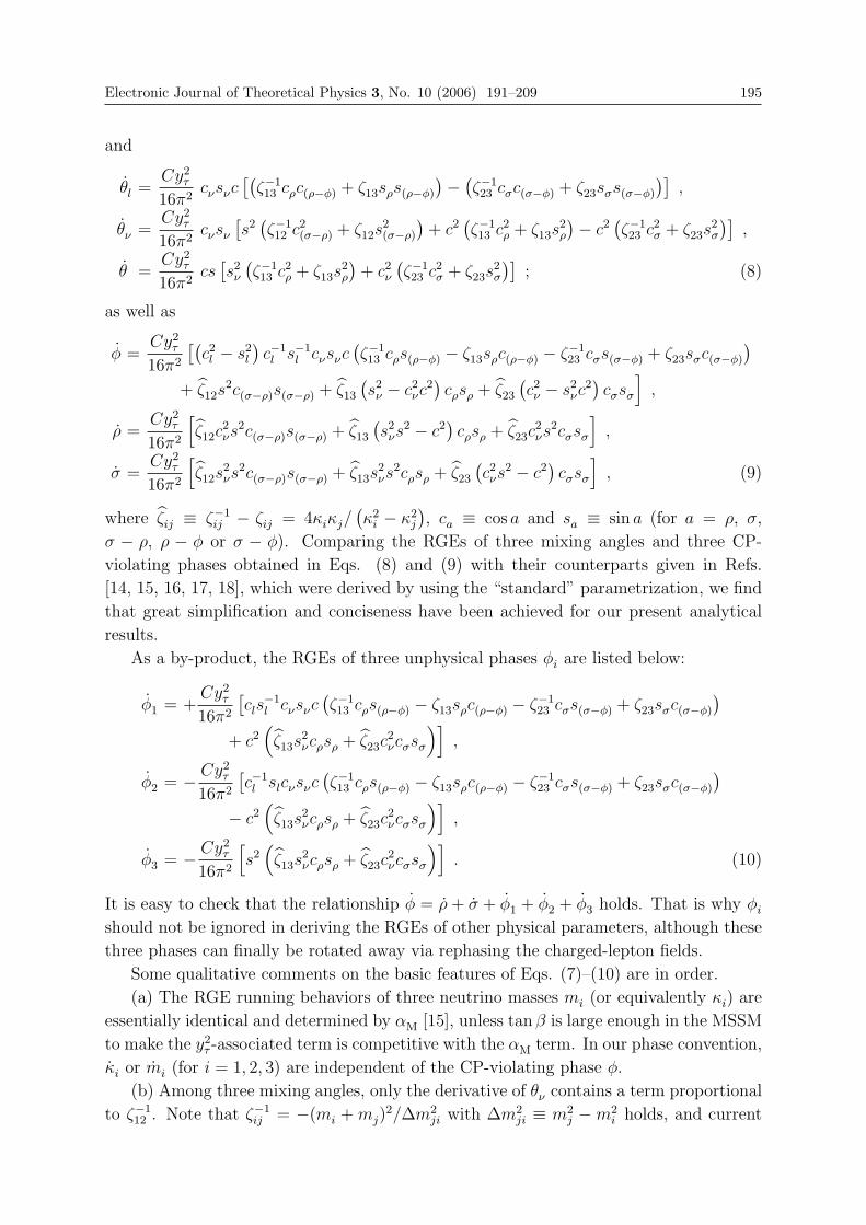
Electronic Journal of Theoretical Physics 3, No. 10 (2006) 191–209 195
and
θl =Cy2
τ
16π2cνsνc
[(ζ−113 cρc(ρ−φ) + ζ13sρs(ρ−φ)
)− (ζ−123 cσc(σ−φ) + ζ23sσs(σ−φ)
)],
θν =Cy2
τ
16π2cνsν
[s2(ζ−112 c2
(σ−ρ) + ζ12s2(σ−ρ)
)+ c2
(ζ−113 c2
ρ + ζ13s2ρ
)− c2(ζ−123 c2
σ + ζ23s2σ
)],
θ =Cy2
τ
16π2cs[s2
ν
(ζ−113 c2
ρ + ζ13s2ρ
)+ c2
ν
(ζ−123 c2
σ + ζ23s2σ
)]; (8)
as well as
φ =Cy2
τ
16π2
[(c2l − s2
l
)c−1l s−1
l cνsνc(ζ−113 cρs(ρ−φ) − ζ13sρc(ρ−φ) − ζ−1
23 cσs(σ−φ) + ζ23sσc(σ−φ)
)+ ζ12s
2c(σ−ρ)s(σ−ρ) + ζ13
(s2
ν − c2νc
2)cρsρ + ζ23
(c2ν − s2
νc2)cσsσ
],
ρ =Cy2
τ
16π2
[ζ12c
2νs
2c(σ−ρ)s(σ−ρ) + ζ13
(s2
νs2 − c2
)cρsρ + ζ23c
2νs
2cσsσ
],
σ =Cy2
τ
16π2
[ζ12s
2νs
2c(σ−ρ)s(σ−ρ) + ζ13s2νs
2cρsρ + ζ23
(c2νs
2 − c2)cσsσ
], (9)
where ζij ≡ ζ−1ij − ζij = 4κiκj/
(κ2
i − κ2j
), ca ≡ cos a and sa ≡ sin a (for a = ρ, σ,
σ − ρ, ρ − φ or σ − φ). Comparing the RGEs of three mixing angles and three CP-
violating phases obtained in Eqs. (8) and (9) with their counterparts given in Refs.
[14, 15, 16, 17, 18], which were derived by using the “standard” parametrization, we find
that great simplification and conciseness have been achieved for our present analytical
results.
As a by-product, the RGEs of three unphysical phases φi are listed below:
φ1 = +Cy2
τ
16π2
[cls
−1l cνsνc
(ζ−113 cρs(ρ−φ) − ζ13sρc(ρ−φ) − ζ−1
23 cσs(σ−φ) + ζ23sσc(σ−φ)
)+ c2
(ζ13s
2νcρsρ + ζ23c
2νcσsσ
)],
φ2 = − Cy2τ
16π2
[c−1l slcνsνc
(ζ−113 cρs(ρ−φ) − ζ13sρc(ρ−φ) − ζ−1
23 cσs(σ−φ) + ζ23sσc(σ−φ)
)− c2
(ζ13s
2νcρsρ + ζ23c
2νcσsσ
)],
φ3 = − Cy2τ
16π2
[s2(ζ13s
2νcρsρ + ζ23c
2νcσsσ
)]. (10)
It is easy to check that the relationship φ = ρ + σ + φ1 + φ2 + φ3 holds. That is why φi
should not be ignored in deriving the RGEs of other physical parameters, although these
three phases can finally be rotated away via rephasing the charged-lepton fields.
Some qualitative comments on the basic features of Eqs. (7)–(10) are in order.
(a) The RGE running behaviors of three neutrino masses mi (or equivalently κi) are
essentially identical and determined by αM [15], unless tan β is large enough in the MSSM
to make the y2τ -associated term is competitive with the αM term. In our phase convention,
κi or mi (for i = 1, 2, 3) are independent of the CP-violating phase φ.
(b) Among three mixing angles, only the derivative of θν contains a term proportional
to ζ−112 . Note that ζ−1
ij = −(mi + mj)2/Δm2
ji with Δm2ji ≡ m2
j −m2i holds, and current
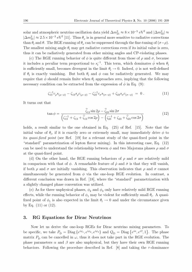
196 Electronic Journal of Theoretical Physics 3, No. 10 (2006) 191–209
solar and atmospheric neutrino oscillation data yield Δm221 ≈ 8×10⁻⁵ eV2 and |Δm2
32| ≈|Δm2
31| ≈ 2.5×10⁻³ eV2 [11]. Thus θν is in general more sensitive to radiative corrections
than θl and θ. The RGE running of θν can be suppressed through the fine-tuning of (σ−ρ).
The smallest mixing angle θl may get radiative corrections even if its initial value is zero,
thus it can be radiatively generated from other mixing angles and CP-violating phases.
(c) The RGE running behavior of φ is quite different from those of ρ and σ, because
it includes a peculiar term proportional to s−1l . This term, which dominates φ when θl
is sufficiently small, becomes divergent in the limit θl → 0. Indeed, φ is not well-defined
if θl is exactly vanishing. But both θl and φ can be radiatively generated. We may
require that φ should remain finite when θl approaches zero, implying that the following
necessary condition can be extracted from the expression of φ in Eq. (9):
ζ−113 cρs(ρ−φ) − ζ13sρc(ρ−φ) − ζ−1
23 cσs(σ−φ) + ζ23sσc(σ−φ) = 0 . (11)
It turns out that
tan φ =ζ13 sin 2ρ− ζ23 sin 2σ(
ζ−113 + ζ13 + ζ13 cos 2ρ
)−(ζ−123 + ζ23 + ζ23 cos 2σ
) (12)
holds, a result similar to the one obtained in Eq. (25) of Ref. [15]. Note that the
initial value of θl, if it is exactly zero or extremely small, may immediately drive φ to
its quasi-fixed point (see Ref. [19] for a relevant study of the quasi-fixed point in the
“standard” parametrization of lepton flavor mixing). In this interesting case, Eq. (12)
can be used to understand the relationship between φ and two Majorana phases ρ and σ
at the quasi-fixed point.
(d) On the other hand, the RGE running behaviors of ρ and σ are relatively mild
in comparison with that of φ. A remarkable feature of ρ and σ is that they will vanish,
if both ρ and σ are initially vanishing. This observation indicates that ρ and σ cannot
simultaneously be generated from φ via the one-loop RGE evolution. In contrast, a
different conclusion was drawn in Ref. [18], where the “standard” parametrization with
a slightly changed phase convention was utilized.
(e) As for three unphysical phases, φ2 and φ3 only have relatively mild RGE running
effects, while the running behavior of φ1 may be violent for sufficiently small θl. A quasi-
fixed point of φ1 is also expected in the limit θl → 0 and under the circumstance given
by Eq. (11) or (12).
3. RG Equations for Dirac Neutrinos
Now let us derive the one-loop RGEs for Dirac neutrino mixing parameters. To
be specific, we take PD = Diag {eiϕ1 , eiϕ2 , eiϕ3} and QD = Diag{eiα, eiβ, 1
}. The phase
matrix PD can be cancelled in ω, thus it does not take part in the RGE evolution. The
phase parameters α and β are also unphysical, but they have their own RGE running
behaviors. Following the procedure described in Ref. [8] and taking the τ -dominance
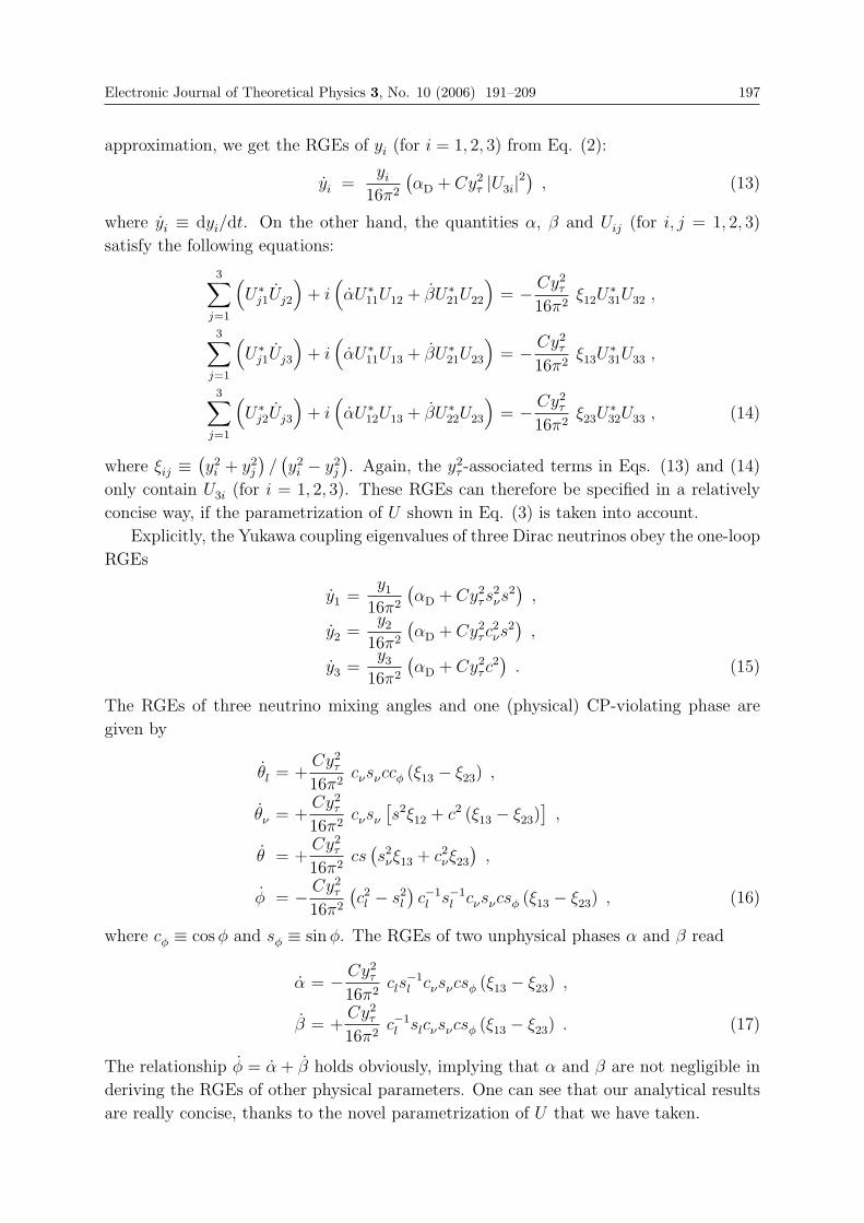
Electronic Journal of Theoretical Physics 3, No. 10 (2006) 191–209 197
approximation, we get the RGEs of yi (for i = 1, 2, 3) from Eq. (2):
yi =yi
16π2
(αD + Cy2
τ |U3i|2)
, (13)
where yi ≡ dyi/dt. On the other hand, the quantities α, β and Uij (for i, j = 1, 2, 3)
satisfy the following equations:
3∑j=1
(U∗
j1Uj2
)+ i
(αU∗
11U12 + βU∗21U22
)= − Cy2
τ
16π2ξ12U
∗31U32 ,
3∑j=1
(U∗
j1Uj3
)+ i
(αU∗
11U13 + βU∗21U23
)= − Cy2
τ
16π2ξ13U
∗31U33 ,
3∑j=1
(U∗
j2Uj3
)+ i
(αU∗
12U13 + βU∗22U23
)= − Cy2
τ
16π2ξ23U
∗32U33 , (14)
where ξij ≡(y2
i + y2j
)/(y2
i − y2j
). Again, the y2
τ -associated terms in Eqs. (13) and (14)
only contain U3i (for i = 1, 2, 3). These RGEs can therefore be specified in a relatively
concise way, if the parametrization of U shown in Eq. (3) is taken into account.
Explicitly, the Yukawa coupling eigenvalues of three Dirac neutrinos obey the one-loop
RGEs
y1 =y1
16π2
(αD + Cy2
τs2νs
2)
,
y2 =y2
16π2
(αD + Cy2
τc2νs
2)
,
y3 =y3
16π2
(αD + Cy2
τc2)
. (15)
The RGEs of three neutrino mixing angles and one (physical) CP-violating phase are
given by
θl = +Cy2
τ
16π2cνsνccφ (ξ13 − ξ23) ,
θν = +Cy2
τ
16π2cνsν
[s2ξ12 + c2 (ξ13 − ξ23)
],
θ = +Cy2
τ
16π2cs(s2
νξ13 + c2νξ23
),
φ = − Cy2τ
16π2
(c2l − s2
l
)c−1l s−1
l cνsνcsφ (ξ13 − ξ23) , (16)
where cφ ≡ cos φ and sφ ≡ sin φ. The RGEs of two unphysical phases α and β read
α = − Cy2τ
16π2cls
−1l cνsνcsφ (ξ13 − ξ23) ,
β = +Cy2
τ
16π2c−1l slcνsνcsφ (ξ13 − ξ23) . (17)
The relationship φ = α + β holds obviously, implying that α and β are not negligible in
deriving the RGEs of other physical parameters. One can see that our analytical results
are really concise, thanks to the novel parametrization of U that we have taken.
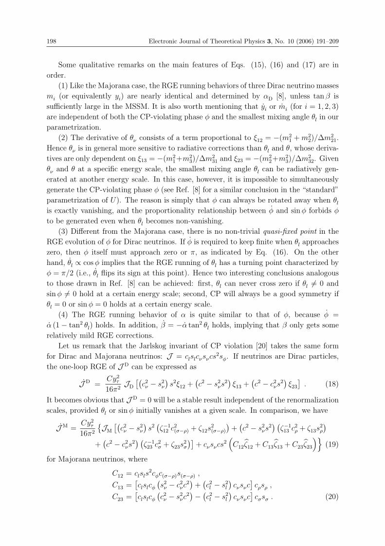
198 Electronic Journal of Theoretical Physics 3, No. 10 (2006) 191–209
Some qualitative remarks on the main features of Eqs. (15), (16) and (17) are in
order.
(1) Like the Majorana case, the RGE running behaviors of three Dirac neutrino masses
mi (or equivalently yi) are nearly identical and determined by αD [8], unless tan β is
sufficiently large in the MSSM. It is also worth mentioning that yi or mi (for i = 1, 2, 3)
are independent of both the CP-violating phase φ and the smallest mixing angle θl in our
parametrization.
(2) The derivative of θν consists of a term proportional to ξ12 = −(m21 + m2
2)/Δm221.
Hence θν is in general more sensitive to radiative corrections than θl and θ, whose deriva-
tives are only dependent on ξ13 = −(m21+m2
3)/Δm231 and ξ23 = −(m2
2+m23)/Δm2
32. Given
θν and θ at a specific energy scale, the smallest mixing angle θl can be radiatively gen-
erated at another energy scale. In this case, however, it is impossible to simultaneously
generate the CP-violating phase φ (see Ref. [8] for a similar conclusion in the “standard”
parametrization of U). The reason is simply that φ can always be rotated away when θl
is exactly vanishing, and the proportionality relationship between φ and sin φ forbids φ
to be generated even when θl becomes non-vanishing.
(3) Different from the Majorana case, there is no non-trivial quasi-fixed point in the
RGE evolution of φ for Dirac neutrinos. If φ is required to keep finite when θl approaches
zero, then φ itself must approach zero or π, as indicated by Eq. (16). On the other
hand, θl ∝ cos φ implies that the RGE running of θl has a turning point characterized by
φ = π/2 (i.e., θl flips its sign at this point). Hence two interesting conclusions analogous
to those drawn in Ref. [8] can be achieved: first, θl can never cross zero if θl �= 0 and
sin φ �= 0 hold at a certain energy scale; second, CP will always be a good symmetry if
θl = 0 or sin φ = 0 holds at a certain energy scale.
(4) The RGE running behavior of α is quite similar to that of φ, because φ =
α (1− tan2 θl) holds. In addition, β = −α tan2 θl holds, implying that β only gets some
relatively mild RGE corrections.
Let us remark that the Jarlskog invariant of CP violation [20] takes the same form
for Dirac and Majorana neutrinos: J = clslcνsνcs2sφ. If neutrinos are Dirac particles,
the one-loop RGE of J D can be expressed as
J D =Cy2
τ
16π2JD
[(c2ν − s2
ν
)s2ξ12 +
(c2 − s2
νs2)ξ13 +
(c2 − c2
νs2)ξ23
]. (18)
It becomes obvious that J D = 0 will be a stable result independent of the renormalization
scales, provided θl or sin φ initially vanishes at a given scale. In comparison, we have
JM =Cy2
τ
16π2
{JM
[(c2ν − s2
ν
)s2(ζ−112 c2
(σ−ρ) + ζ12s2(σ−ρ)
)+(c2 − s2
νs2) (
ζ−113 c2
ρ + ζ13s2ρ
)+(c2 − c2
νs2) (
ζ−123 c2
σ + ζ23s2σ
)]+ cνsνcs
2(C12ζ12 + C13ζ13 + C23ζ23
)}(19)
for Majorana neutrinos, where
C12 = clsls2cφc(σ−ρ)s(σ−ρ) ,
C13 =[clslcφ
(s2
ν − c2νc
2)
+(c2l − s2
l
)cνsνc
]cρsρ ,
C23 =[clslcφ
(c2ν − s2
νc2)− (c2
l − s2l
)cνsνc
]cσsσ . (20)
Electronic Journal of Theoretical Physics 3, No. 10 (2006) 191–209 199
One can see that JM can be radiatively generated from two non-trivial Majorana phases
ρ and σ, even if it is initially vanishing at a specific scale. Taking ρ = σ = 0, we
arrive at C12 = C13 = C23 = 0 as well as ρ = σ = 0. But it is impossible to obtain
the equality JM(ρ = σ = 0) = J D, because ζ−112 = ξ12, ζ−1
13 = ξ13 and ζ−123 = ξ23 (or
equivalently m1m2 = m1m3 = m2m3 = 0) cannot simultaneously hold. This observation
demonstrates again that the RGE running behavior of JM is essentially different from
that of J D.
4. Comparison Between Dirac and Majorana Neutrinos
The one-loop RGEs for three Yukawa coupling eigenvalues of Dirac neutrinos (yi
with i = 1, 2, 3) and their four flavor mixing parameters (θl, θν , θ and φ) have been
derived above. Here we replace yi by mi. The RGEs of three neutrino masses, three
mixing angles and one CP-violating phase can then be written as
m1 =m1
16π2
(αD + Cy2
τs2νs
2)
,
m2 =m2
16π2
(αD + Cy2
τc2νs
2)
,
m3 =m3
16π2
(αD + Cy2
τc2)
; (21)
and
θl = +Cy2
τ
8π2cνsνccφ
m23 (m2
2 −m21)
(m23 −m2
1) (m23 −m2
2),
θν = − Cy2τ
16π2cνsν
[s2 m2
2 + m21
m22 −m2
1
− c2 2m23 (m2
2 −m21)
(m23 −m2
1) (m23 −m2
2)
],
θ = − Cy2τ
16π2cs
(s2
ν
m23 + m2
1
m23 −m2
1
+ c2ν
m23 + m2
2
m23 −m2
2
),
φ = −Cy2τ
8π2
(c2l − s2
l
)c−1l s−1
l cνsνcsφ
m23 (m2
2 −m21)
(m23 −m2
1) (m23 −m2
2). (22)
Note that the neutrino mass-squared differences Δm231 and Δm2
32 are much larger in
magnitude than Δm221, as indicated by current experimental data. Typically, Δm2
21 ≈8.0 × 10⁻⁵ eV2 and |Δm2
31| ≈ |Δm232| ≈ 2.5 × 10⁻³ eV2 [11]. Among three neutrino
mixing angles, the RGE running of θν is expected to be most significant. The CP-
violating phase φ may significantly evolve from one energy scale to another, if θl takes
sufficiently small values. These qualitative features will become clearer in our subsequent
numerical calculations.
The one-loop RGEs for three effective coupling eigenvalues of Majorana neutrinos (κi
with i = 1, 2, 3) and their six flavor mixing parameters (θl, θν , θ, φ, ρ and σ) have been
presented in section II. Here we replace κi by mi and take ρ = σ = 0 at either ΛEW or
ΛSS. As one can see from Eq. (9), ρ = σ = 0 leads to ρ = σ = 0. In other words, two
Majorana phases ρ and σ keep vanishing at any energy scales between ΛEW and ΛSS. One
may safely simplify the RGEs of θl, θν , θ and φ obtained in Eqs. (8) and (9) by setting
200 Electronic Journal of Theoretical Physics 3, No. 10 (2006) 191–209
ρ = σ = 0, and then compare them with their Dirac counterparts on the same footing.
In this case, we arrive at
m1 =m1
16π2
(αM + 2Cy2
τs2νs
2)
,
m2 =m2
16π2
(αM + 2Cy2
τc2νs
2)
,
m3 =m3
16π2
(αM + 2Cy2
τc2)
; (23)
and
θl = +Cy2
τ
8π2cνsνccφ
m3(m2 −m1)
(m3 −m1) (m3 −m2),
θν = − Cy2τ
16π2cνsν
[s2 m2 + m1
m2 −m1
− c2 2m3 (m2 −m1)
(m3 −m1) (m3 −m2)
],
θ = − Cy2τ
16π2cs
(s2
ν
m3 + m1
m3 −m1
+ c2ν
m3 + m2
m3 −m2
),
φ = −Cy2τ
8π2
(c2l − s2
l
)c−1l s−1
l cνsνcsφ
m3 (m2 −m1)
(m3 −m1) (m3 −m2). (24)
As a consequence of Δm221 � |Δm2
31| ≈ |Δm232|, the mixing angle θν is most sensitive to
radiative corrections. The RGE evolution of the CP-violating phase φ depends strongly
on the smallness of θl, on the other hand. These qualitative features are essentially
analogous to what we have pointed out for Dirac neutrinos.
It is interesting to note that Eq. (23) can actually be obtained from Eq. (21) with
the replacements αD =⇒ αM and C =⇒ 2C, while Eq. (24) can be achieved from Eq.
(22) with the replacements m2i =⇒ mi (for i = 1, 2, 3). These similarities and differences
imply that it is very non-trivial to distinguish between the RGE running behaviors of
Dirac neutrinos and Majorana neutrinos with vanishing Majorana CP-violating phases.Taking ρ = σ = 0 in the Majorana case, we obtain a simplified expression of JM,
JM =Cy2
τ
16π2JM
[(c2ν − s2
ν
)s2 m2 + m1
m2 −m1
+(c2 − s2
νs2) m3 + m1
m3 −m1
+(c2 − c2
νs2) m3 + m2
m3 −m2
],
(25)which is very analogous to J D of Dirac neutrinos,
J D =Cy2
τ
16π2J D
[(c2ν − s2
ν
)s2 m2
2 + m21
m22 −m2
1
+(c2 − s2
νs2) m2
3 + m21
m23 −m2
1
+(c2 − c2
νs2) m2
3 + m22
m23 −m2
2
].
(26)
It is obvious that Eq. (26) can be obtained from Eq. (25) with the replacements mi =⇒m2
i (for i = 1, 2, 3). Note that J D ∝ J D (or JM ∝ JM) holds. This result implies that
the Jarlskog parameter will keep vanishing at any energy scales between ΛEW and ΛSS,
if it initially vanishes at either ΛEW or ΛSS.
Because αM > αD and (mj + mi)/(mj − mi) > (m2j + m2
i )/(m2j − m2
i ) hold (for
mj > mi), the RGE running of each Majorana neutrino parameter is in general expected
to be faster (i.e., more significant) than the RGE running of the corresponding Dirac
neutrino parameter.
Electronic Journal of Theoretical Physics 3, No. 10 (2006) 191–209 201
5. Numerical Results
In view of the fact that the absolute mass scale of three light neutrinos and the sign
of Δm232 remain unknown at present, let us consider four typical patterns of the neutrino
mass spectrum:
• Normal hierarchy (NH): m1 � m2 � m3. For simplicity, we typically take m1 = 0 at
ΛEW in our numerical calculations. Then m2 =√
Δm221 and m3 =
√|Δm232|+ Δm2
21
can be determined from current experimental data.
• Inverted hierarchy (IH): m3 � m1 � m2. For simplicity, w typically take m3 = 0 at
ΛEW in our numerical calculations. Then m2 =√|Δm2
32| and m1 =√|Δm2
32| −Δm221
can be determined from current experimental data.
• Near degeneracy (ND) with Δm232 > 0: m1 � m2 � m3. For simplicity, we typically
take m1 = 0.2 eV at ΛEW in our numerical calculations.
• Near degeneracy (ND) with Δm232 < 0: m3 � m1 � m2. For simplicity, we typically
take m1 = 0.2 eV at ΛEW in our numerical calculations.
In addition, we take Δm221 = 8.0×10⁻⁵ eV2, |Δm2
32| = 2.5×10⁻³ eV2, θν = 33.8◦, θ = 45◦,θl = 0.5◦ and φ = 90◦ as typical inputs at ΛEW ∼MZ in our numerical calculations [13].
5.1 Neutrino Masses
In either the SM or the MSSM with small tan β, the RGE running behaviors of three
neutrino masses are dominated by αD or αM. The y2τ -associated term of m2
i in Eq. (21)
or (23) becomes important only when tan β takes sufficiently large values in the MSSM
[14, 15, 16, 17]. Note that αM = 2αD holds in the MSSM, in which the running effects of
mi for Majorana neutrinos are twice as large as those for Dirac neutrinos.
The first plot in Fig. 1 illustrates the ratios Ri ≡ mi(μ)/mi(MZ) changing with the
energy scale μ in the SM for Dirac and Majorana neutrinos, where m1(MZ) = 0.2 eV
and MH = 180 GeV (the Higgs mass) have typically been input. Since the running
of mi is governed by αD or αM, R1 ≈ R2 ≈ R3 holds to a high degree of accuracy.
Furthermore, the behaviors of Ri are actually independent of the initial value of m1 and
possible patterns of the neutrino mass spectrum. We observe that Ri in the Majorana
case is always larger than Ri in the Dirac case, and their discrepancy can be as large as
0.7 at μ ∼ ΛSS ∼ 1014 GeV.
The relation R1 ≈ R2 ≈ R3 is also a very good approximation in the MSSM with
small tan β, as shown by the second plot in Fig. 1, where tan β = 10 has been input. It
is clear that Ri in the Dirac case is numerically distinguishable from Ri in the Majorana
case, in particular when the energy scale μ far exceeds MZ .
If tan β is sufficiently large, the common scaling of three neutrino masses in the RGE
evolution will fail [15]. The splitting of R1, R2 and R3, which increases with the energy
scale μ, is illustrated by the third plot in Fig. 1 with the input tan β = 50. One can
202 Electronic Journal of Theoretical Physics 3, No. 10 (2006) 191–209
see that Ri in the Dirac case is always smaller than Ri in the Majorana case, and their
discrepancy is distinguishable at the scales μ!MZ .
5.2 Neutrino Mixing Parameters
Radiative corrections to three neutrino mixing angles, the Dirac CP-violating phase and
the Jarlskog parameter are all controlled by the τ -lepton Yukawa coupling eigenvalue yτ .
Because of y2τ/(8π
2) ≈ 1.3 × 10⁻⁶ (SM) or y2τ/(8π2) ≈ 1.3 × 10⁻⁶ (1 + tan2 β) (MSSM)
at MZ , significant RGE running effects are expected to appear in the MSSM case when
tan β is sufficiently large. To illustrate, here we simply concentrate on the MSSM with
tan β = 50 and consider four typical patterns of the neutrino mass spectrum in our
subsequent discussions and calculations.
(1) In the NH case with m1 = 0, the RGEs of θl, θν , θ, φ and J can be simplified as
θl = +Cy2
τ
16π2cνsνccφr , θν = − Cy2
τ
16π2cνsν
(s2 − c2r
),
θ = − Cy2τ
16π2cs (1 + r) , φ = − Cy2
τ
16π2
(c2l − s2
l
)c−1l s−1
l cνsνcsφr ,
J =Cy2
τ
16π2J [2 (s2
νs2 − c2
)− (c2 − c2νs
2)r]
, (27)
in which r = 2m22/(m
23 −m2
2) for Dirac neutrinos or r = 2m2/(m3 −m2) for Majorana
neutrinos. Current experimental data yield rD ≈ 0.06 and rM ≈ 0.4. Both of them are
too small to compensate for the strong suppression induced by y2τ in Eq. (27). Thus the
RGE corrections to those flavor mixing and CP-violating parameters are not important
in the NH case. Note, however, that the radiative correction to φ can be very significant
when θl is extremely small or becomes vanishing. We find that φ quickly approaches its
quasi-fixed point φQF = 0 or π in the θl → 0 limit, an interesting phenomenon which is
remarkably different from the non-trivial quasi-fixed point of φ discovered in the general
(ρ �= σ �= 0) case for Majorana neutrinos [19]. One can also see that both J = 0 and
J = 0 hold when θl vanishes; i.e., CP is a good symmetry in this limit.
(2) In the IH case with m3 = 0, we arrive at
θl = φ = 0, θν = − Cy2τ
16π2cνsνs
2r′ , θ = +Cy2
τ
16π2cs ,
J =Cy2
τ
16π2J [3c2 − 1 +
(s2
ν − c2ν
)s2r′
], (28)
where r′ = (m22 + m2
1)/(m22 −m2
1) for Dirac neutrinos or r′ = (m2 + m1)/(m2 −m1) for
Majorana neutrinos. We observe that radiative corrections to θl and φ are vanishingly
small, and the correction to θ is also insignificant. Nevertheless, the RGE running effects
of θν and J may get enhanced by r′, whose typical value reads r′D ≈ 60 or r′M ≈ 120 at
MZ . Fig. 2 illustrates the evolution of θν and J in the IH case. The discrepancy between
Dirac and Majorana cases is obviously distinguishable for both parameters, when the
energy scale is much higher than MZ . In particular, J D ∼ 2JM holds at μ ∼ ΛSS,
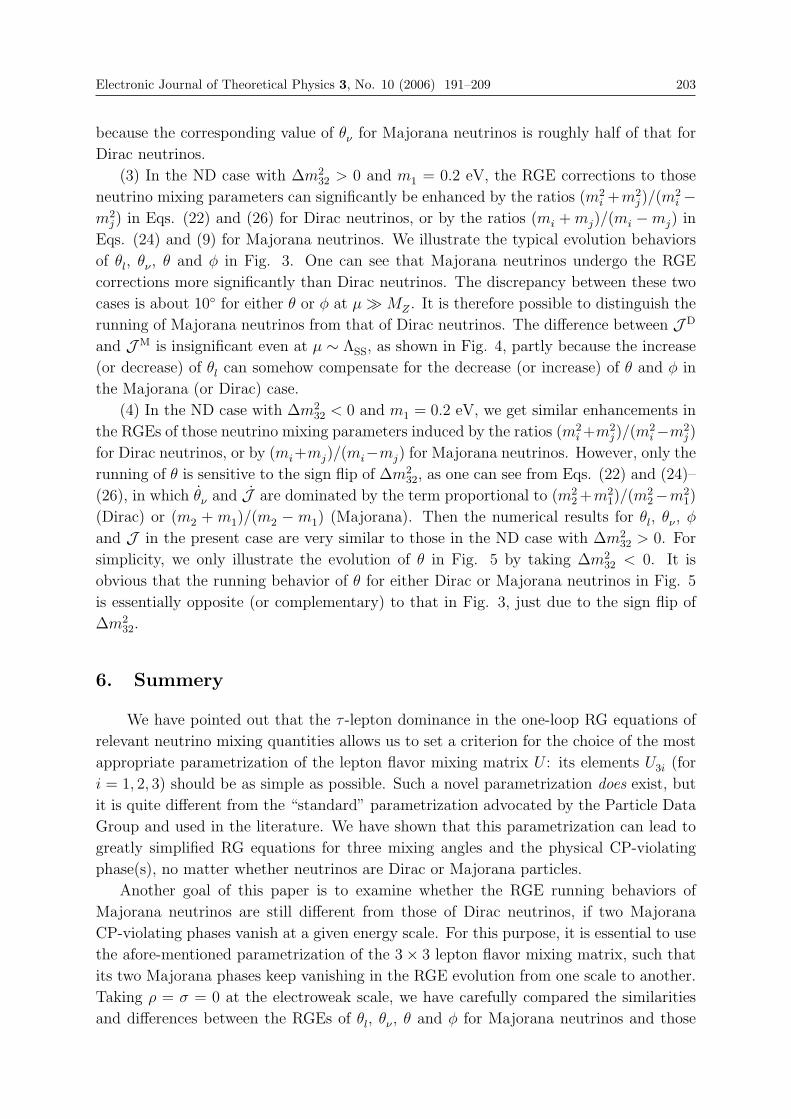
Electronic Journal of Theoretical Physics 3, No. 10 (2006) 191–209 203
because the corresponding value of θν for Majorana neutrinos is roughly half of that for
Dirac neutrinos.
(3) In the ND case with Δm232 > 0 and m1 = 0.2 eV, the RGE corrections to those
neutrino mixing parameters can significantly be enhanced by the ratios (m2i +m2
j)/(m2i −
m2j) in Eqs. (22) and (26) for Dirac neutrinos, or by the ratios (mi + mj)/(mi −mj) in
Eqs. (24) and (9) for Majorana neutrinos. We illustrate the typical evolution behaviors
of θl, θν , θ and φ in Fig. 3. One can see that Majorana neutrinos undergo the RGE
corrections more significantly than Dirac neutrinos. The discrepancy between these two
cases is about 10◦ for either θ or φ at μ!MZ . It is therefore possible to distinguish the
running of Majorana neutrinos from that of Dirac neutrinos. The difference between J D
and JM is insignificant even at μ ∼ ΛSS, as shown in Fig. 4, partly because the increase
(or decrease) of θl can somehow compensate for the decrease (or increase) of θ and φ in
the Majorana (or Dirac) case.
(4) In the ND case with Δm232 < 0 and m1 = 0.2 eV, we get similar enhancements in
the RGEs of those neutrino mixing parameters induced by the ratios (m2i +m2
j)/(m2i−m2
j)
for Dirac neutrinos, or by (mi+mj)/(mi−mj) for Majorana neutrinos. However, only the
running of θ is sensitive to the sign flip of Δm232, as one can see from Eqs. (22) and (24)–
(26), in which θν and J are dominated by the term proportional to (m22 +m2
1)/(m22−m2
1)
(Dirac) or (m2 + m1)/(m2 − m1) (Majorana). Then the numerical results for θl, θν , φ
and J in the present case are very similar to those in the ND case with Δm232 > 0. For
simplicity, we only illustrate the evolution of θ in Fig. 5 by taking Δm232 < 0. It is
obvious that the running behavior of θ for either Dirac or Majorana neutrinos in Fig. 5
is essentially opposite (or complementary) to that in Fig. 3, just due to the sign flip of
Δm232.
6. Summery
We have pointed out that the τ -lepton dominance in the one-loop RG equations of
relevant neutrino mixing quantities allows us to set a criterion for the choice of the most
appropriate parametrization of the lepton flavor mixing matrix U : its elements U3i (for
i = 1, 2, 3) should be as simple as possible. Such a novel parametrization does exist, but
it is quite different from the “standard” parametrization advocated by the Particle Data
Group and used in the literature. We have shown that this parametrization can lead to
greatly simplified RG equations for three mixing angles and the physical CP-violating
phase(s), no matter whether neutrinos are Dirac or Majorana particles.
Another goal of this paper is to examine whether the RGE running behaviors of
Majorana neutrinos are still different from those of Dirac neutrinos, if two Majorana
CP-violating phases vanish at a given energy scale. For this purpose, it is essential to use
the afore-mentioned parametrization of the 3× 3 lepton flavor mixing matrix, such that
its two Majorana phases keep vanishing in the RGE evolution from one scale to another.
Taking ρ = σ = 0 at the electroweak scale, we have carefully compared the similarities
and differences between the RGEs of θl, θν , θ and φ for Majorana neutrinos and those
204 Electronic Journal of Theoretical Physics 3, No. 10 (2006) 191–209
for Dirac neutrinos. Our numerical calculations show that it is possible to distinguish
between these two cases in the MSSM with sizable tan β, in particular when the masses
of three neutrinos are nearly degenerate or have an inverted hierarchy. Furthermore,
we conclude that Majorana neutrinos are in general expected to run faster (i.e., more
significantly) than Dirac neutrinos from one energy scale to another.
Of course, the numerical examples presented in this work are mainly for the purpose
of illustration. The point is that the nature of neutrinos determines their RGE running
behaviors, and the latter may be crucial for building a realistic neutrino model. We
expect that our analysis can not only complement those previous studies of radiative
corrections to the physical parameters of Dirac and Majorana neutrinos, but also help
us understand the dynamical role of Majorana phases in a more general picture of flavor
physics.
This work is supported in part by the National Nature Science Foundation of China.
Electronic Journal of Theoretical Physics 3, No. 10 (2006) 191–209 205
References
[1] SNO Collaboration, Q.R. Ahmad et al., Phys. Rev. Lett. 89, 011301 (2002).
[2] For a review, see: C.K. Jung et al., Ann. Rev. Nucl. Part. Sci. 51, 451 (2001).
[3] KamLAND Collaboration, K. Eguchi et al., Phys. Rev. Lett. 90, 021802 (2003);CHOOZ Collaboration, M. Apollonio et al., Phys. Lett. B 420, 397 (1998); PaloVerde Collaboration, F. Boehm et al., Phys. Rev. Lett. 84, 3764 (2000).
[4] K2K Collaboration, M.H. Ahn et al., Phys. Rev. Lett. 90, 041801 (2003).
[5] For recent reviews with extensive references, see: H. Fritzsch and Z.Z. Xing, Prog.Part. Nucl. Phys. 45, 1 (2000); S.F. King, Rept. Prog. Phys. 67, 107 (2004); G.Altarelli and F. Feruglio, New J. Phys. 6, 106 (2004); R.N. Mohapatra et al., hep-ph/0510213.
[6] P. Minkowski, Phys. Lett. B 67, 421 (1977); T. Yanagida, in Proceedings of theWorkshop on Unified Theory and the Baryon Number of the Universe, edited by O.Sawada and A. Sugamoto (KEK, Tsukuba, 1979), p. 95; M. Gell-Mann, P. Ramond,and R. Slansky, in Supergravity, edited by F. van Nieuwenhuizen and D. Freedman(North Holland, Amsterdam, 1979), p. 315; S.L. Glashow, in Quarks and Leptons,edited by M. Levy et al. (Plenum, New York, 1980), p. 707; R.N. Mohapatra and G.Senjanovic, Phys. Rev. Lett. 44, 912 (1980).
[7] P.H. Chankowski and Z. Pluciennik, Phys. Lett. B 316, 312 (1993); K.S. Babu, C.N.Leung, and J. Pantaleone, Phys. Lett. B 319, 191 (1993); S. Antusch, M. Drees, J.Kersten, M. Lindner, and M. Ratz, Phys. Lett. B 519, 238 (2001); Phys. Lett. B525, 130 (2002).
[8] M. Lindner, M. Ratz, and M.A. Schmidt, hep-ph/0506280; and references therein.
[9] Particle Data Group, S. Eidelman et al., Phys. Lett. B 592, 1 (2004).
[10] H. Fritzsch and Z.Z. Xing, Phys. Lett. B 413, 396 (1997); Phys. Rev. D 57, 594(1998).
[11] See, e.g., M. Maltoni, T. Schwetz, M.A. Tortola, and J.W.F. Valle, New. J. Phys. 6,122 (2004); A. Strumia and F. Vissani, Nucl. Phys. B 726, 294 (2005).
[12] Z.Z. Xing, Phys. Lett. B 633, 550 (2006).
[13] Z.Z. Xing and H. Zhang, hep-ph/0601106.
[14] J.A. Casas, J.R. Espinosa, A. Ibarra, and I. Navarro, Nucl. Phys. B 573, 652 (2000).
[15] S. Antusch, J. Kersten, M. Lindner, and M. Ratz, Nucl. Phys. B 674, 401 (2003).
[16] S. Antusch, J. Kersten, M. Lindner, M. Ratz, and M.A. Schmidt, JHEP 0503, 024(2005).
[17] J.W. Mei, Phys. Rev. D 71, 073012 (2005).
[18] S. Luo, J. Mei, and Z.Z. Xing, Phys. Rev. D 72, 053014 (2005).
[19] S. Luo and Z.Z. Xing, Phys. Lett. B 632, 341 (2006).
[20] C. Jarlskog, Phys. Rev. Lett. 55, 1039 (1985); Z.Z. Xing, Int. J. Mod. Phys. A 19, 1(2004).
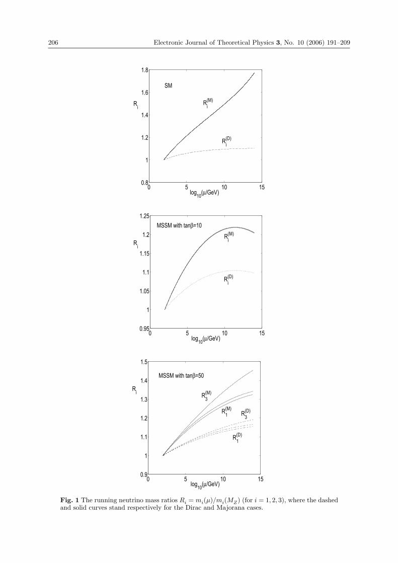
206 Electronic Journal of Theoretical Physics 3, No. 10 (2006) 191–209
0 5 10 150.8
1
1.2
1.4
1.6
1.8
log10(μ/GeV)
SM
R(M)i
R(D)i
Ri
0 5 10 150.95
1
1.05
1.1
1.15
1.2
1.25MSSM with tanβ=10
R(M)i
R(D)i
log10(μ/GeV)
Ri
0 5 10 150.9
1
1.1
1.2
1.3
1.4
1.5
log10(μ/GeV)
R(M)1
R(M)3
R(D)1
R(D)3
MSSM with tanβ=50
Ri
Fig. 1 The running neutrino mass ratios Ri = mi(μ)/mi(MZ) (for i = 1, 2, 3), where the dashedand solid curves stand respectively for the Dirac and Majorana cases.
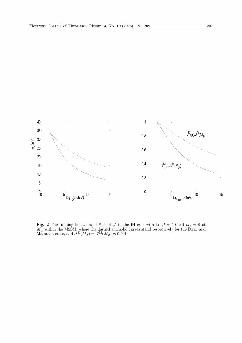
Electronic Journal of Theoretical Physics 3, No. 10 (2006) 191–209 207
0 5 10 150
5
10
15
20
25
30
35
40
log10(μ/GeV)
θν(μ
)/°
0 5 10 150
0.2
0.4
0.6
0.8
1
log10(μ/GeV)
JD(μ)/JD(MZ)
JM(μ)/JM(MZ)
Fig. 2 The running behaviors of θν and J in the IH case with tan β = 50 and m3 = 0 atMZ within the MSSM, where the dashed and solid curves stand respectively for the Dirac andMajorana cases, and J D(MZ) = JM(MZ) ≈ 0.0014.
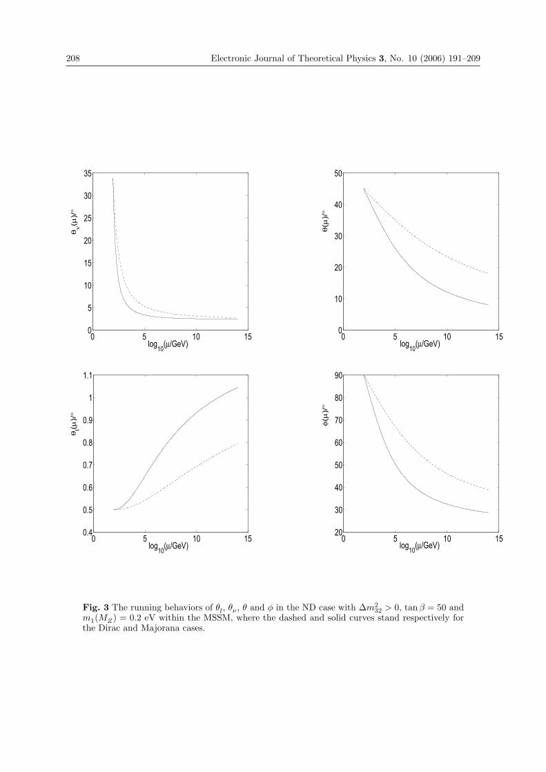
208 Electronic Journal of Theoretical Physics 3, No. 10 (2006) 191–209
0 5 10 150
5
10
15
20
25
30
35
θν(μ
)/°
log10(μ/GeV)0 5 10 15
0
10
20
30
40
50
θ(μ
)/°
log10(μ/GeV)
0 5 10 150.4
0.5
0.6
0.7
0.8
0.9
1
1.1
θl(μ
)/°
log10(μ/GeV)0 5 10 15
20
30
40
50
60
70
80
90
φ(μ
)/°
log10(μ/GeV)
Fig. 3 The running behaviors of θl, θν , θ and φ in the ND case with Δm232 > 0, tan β = 50 and
m1(MZ) = 0.2 eV within the MSSM, where the dashed and solid curves stand respectively forthe Dirac and Majorana cases.
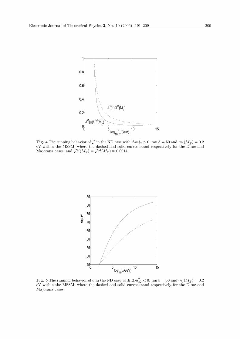
Electronic Journal of Theoretical Physics 3, No. 10 (2006) 191–209 209
0 5 10 150
0.2
0.4
0.6
0.8
1
JM(μ)/JM(MZ)
JD(μ)/JD(MZ)
log10(μ/GeV)
Fig. 4 The running behavior of J in the ND case with Δm232 > 0, tan β = 50 and m1(MZ) = 0.2
eV within the MSSM, where the dashed and solid curves stand respectively for the Dirac andMajorana cases, and J D(MZ) = JM(MZ) ≈ 0.0014.
0 5 10 1545
50
55
60
65
70
75
80
85
log10(μ/GeV)
θ(μ
)/°
Fig. 5 The running behavior of θ in the ND case with Δm232 < 0, tanβ = 50 and m1(MZ) = 0.2
eV within the MSSM, where the dashed and solid curves stand respectively for the Dirac andMajorana cases.
EJTP 3, No. 10 (2006) 211–224 Electronic Journal of Theoretical Physics
Universe Without SingularitiesA Group Approach to De Sitter Cosmology
Ignazio Licata ∗†
IxtuCyber for Complex Systemsvia Favorita 9, 91025, Marsala (TP), Italy
Received 21 May 2006, Published 28 May 2006
Abstract: In the last years the traditional scenario of “Big Bang” has been deeply modified bythe study of the quantum features of the Universe evolution, proposing again the problemof using “local” physical laws on cosmic scale, with particular regard to the cosmologicalconstant role. The “group extention” method shows that the De Sitter group univocallygeneralizes the Poincare group, formally justifies the cosmological constant use and suggestsa new interpretation for Hartle-Hawking boundary conditions in Quantum Cosmology.c© Electronic Journal of Theoretical Physics. All rights reserved.
Keywords: Group Methods in Theoretical Physics, Projective Relativity, De Sitter Universe,Quantum Cosmology.PACS (2006): 02.20.Bb, 02.20.Qs, 02.40.-k, 03.30.+p, 04.90.+e, 98.80.Qc
1. Introduction
There are strong theoretical coherence reasons which impose to critically reconsider
the approach to cosmological problem on the whole. The Quantum Cosmology’s main
problem is to individuate the proper boundary conditions for the Universe’s wave func-
tion in the Wheeler-DeWitt equation. These conditions have to be such to allow the
confrontation between a probability distribution of states and the observed Universe. In
particular, it is expected to select a path in the configuration space able to solve the still
open problems of the Big-Bang traditional scenario: flat space, global homogeneity (hori-
zon problem) and the “ruggedness” necessary to explain the tiny initial dishomogeneities
which have led to the formation of the galactic structures.
The inflationary cosmology ideas has partly supplied with a solution to the standard
212 Electronic Journal of Theoretical Physics 3, No. 10 (2006) 211–224
model wants by introducing the symmetry breaking and phase transition notions which
are at the core of Quantum Cosmology. The last one also finds its motivation in the
necessity to provide with a satisfactory physical meaning to the initial singularity problem,
unavoidable in GR under the condition of the Hawking-Penrose theorem (Hawking &
Ellis, 1973).
The Hartle-Hawking “no-boundary” condition seems to provide a very powerful con-
straint for the Quantum Cosmology main requirements, but appears as an “ad hoc”
solution which could be deduced by a fundamental approach. Particularly, the mix of
topologies used to conciliate without boundary Universe symmetry with the Big-Bang
evolutionary scenario is unsatisfactory.
We realize that most part of the Quantum Cosmology problems inherit the uncertain-
ties of the Fridman model in GR, so they derive from the euristic use of the local laws
on cosmic scale.
A possible way-out is the Fantappie-Arcidiacono group approach which allows to in-
dividuate a Universe model without recourse to arbitrary extrapolations of the symmetry
groups valid in physics.
The group extension theory naturally finds again the Hartle-Hawking condition on
the Universe wave function and allows to firmly founding theoretically the Quantum
Cosmology. The price to pay is a subtle methodological question on using the GR in
cosmology. In fact, in 1952 Fantappie pointed out that the problem of the use of local
laws to define the cosmological boundary conditions is due to the fact that GR describes
matter in terms of local curvature, but leaves the question of space-time global structure
indeterminate. It happens because, differently from RR, GR has not be built on group
base, which thing should be central in building any theory up, especially when it aims to
express universally valid statements on physical world, the class of the superb theories,
how Roger Penrose called them.
We are going to examine here the foundations of the group extension method (par.
2) and the relativity in the De Sitter Universe (par. 3, 4), we introduce the conditions
to define matter-fields (par.5).In (par.6) we analyze the physical significance of the ob-
servers in an istantonic Universe at imaginary time, and in (par.7) investigate the physical
meaning of the Hartle-Hawking condition in an hyper-spherical universe.
2. An Erlangen Program for Cosmology
In 1872 Felix Klein presented the so-called Erlangen program for geometry, centred
upon the symmetry transformations group. From 1952, Fantappie, basing on a similar
idea and in perfect consonance with Relativity spirit, proposed an Erlangen program for
physics, where a Universe is univocally individuated by a symmetry group which let its
physical laws invariant (Fantappie,1954, 1959). It has to be underlined that in the theory
Universe means any physical system characterized by a symmetry group.
The space-time isotropy and homogeneity principle with respect to physical laws tells
us that the physical law concept itself is based upon symmetry. So the essential idea
Electronic Journal of Theoretical Physics 3, No. 10 (2006) 211–224 213
is to individuate physical laws starting from the transformations group which let them
invariant. We observe here that there are infinite possible transformations group which
individuate an isotropic and homogeneous space-time. In order to build the next improve-
ments in physics using the group extension method, we can follow the path indicated by
the two groups we know to be two valid description levels of the physical world: the
Galilei group and the Lorentz-Poincare one. It is useful to remember that the Galilei
group is a particular case of the Lorentz one when c→∞,i.e. when it is not made use of
the field notion and the interactions velocity is considered to be infinite. Staying within
a quadrimensional space-time and consequently considering only groups at 10 parame-
ters and continuous transformations, Fantappie showed that the Poincare group can be
considered a limit case of a broader group depending with continuity on c and another
parameter r: the Fantappie group; moreover this group cannot be further extended under
the condition to stay within a group at 10 parameters.
So we have the sequence:
G101+3 → L10
1+3 → F 101+3
Where G is the Galilei group, L the Lorentz one and F the Fantappie final one, from
which with R → ∞, we get the L group. It is shown that such sequence of universes is
univocal.
The Lorentz group can be mathematically interpreted as the group of roto-translations
such to let that particular object that is the Minkowski space-time invariant. Similarly,
the Fantappie group is the one of the pentadimensional rotations of a new space-time:
the hyper-spherical and at constant curvature De Sitter universe (maximally symmetric).
We point out we have obtained the De Sitter model without referring to the gravitational
interaction, differently from the GR where the De Sitter universe is one of the possible
solutions of the Einstein equations with cosmological constant. From a formal viewpoint
we make recourse to pentadimensional rotations because in the De Sitter universe there
appears a new constant r, which can be interpreted as the Universe radius.
The group extension mechanism individuates an univocal sequence of symmetry
groups; for each symmetry group we have a corresponding level of physical world descrip-
tion and a new universal constant, so providing the most general boundary conditions and
constraining the form of the possibile physical laws. The Fantappie group fixes the c and
rconstants and defines a new relativity for the inertial observers in De Sitter Universe.
In this sense, the Theory of Universes- based on group extension method- is actually a
version of what is sought for in the Holographic Principle: the possibility to describe laws
and boundaries in a compact and unitary way.
In 1956 G. Arcidiacono proposed to study the De Sitter S4 absolute universe by means
of the tangent relative spaces where observers localize and describe the physical events
by using the Beltrami-Castelnuovo P 4 projective representation in the Projective Special
Relativity, PSR (Arcidiacono,1956; 1976; 1984).
We note that we pass from hyper-spherical S4 to its real representation as hyperboloid
by means of an inverse Wick rotation, rotating it → τ and associating the great circles
on the hyper-sphere with a family of geodesics on the hyperboloid. In this way, we get a
214 Electronic Journal of Theoretical Physics 3, No. 10 (2006) 211–224
realization of the Weyl Principle for defining a Universe model, because it fixes a set of
privileged observers (Ellis & Williams, 1988). So, the choice of P 4Beltrami-Castelnuovo
is equivalent to study a relativity in S4.
3. The Fantappie Group Transformations
To study the De Sitter S4 universe according to Beltrami-Castelnuovo representation
we have to set the projectivities which let the Cayley-Klein interval invariant:
x2 + y2 + z2 − c2t2 + r2 = 0 (3.1)
The (3.1) meets the time axis in the two t = ±t0 “singularities”, where t0 = r/c is the
time it takes light to run the Universe r radius. In this case the singularities’ meaning
is purely geometrical, not physical, and they represent the hyperboloid rims (3.1), since
the De Sitter universe is lacking in “structural” singularities. The S4 invariant transfor-
mations are the 5-dimensional space rotations which lead on the P 4 observer’s space the
projectivities that let the (3.1) unchanged.
Let’s introduce the five homogeneous projective coordinates (Weierstrass condition):
xa xa = r2, with a = 0, 1, 2, 3, 4 (3.2)
The xi space-time coordinates, with i = 1,2,3,4 are:
x1 = x, x2 = y, x3 = z, x4 = ict (3.3)
The connection between the (3.2) and (3.3) is given by the relation:
xi = rxi/x0 (3.4)
from which, owing to (3.2), we get the inverse relation:
x0 = r/a, xi = xi/a, (3.5)
where a2 = 1 + xixi/r2 = 1 + α2 − γ2 , with �α = �x/r and γ = t/t0.
The searched transformation between the two O′and O observers consequently has
the form:
x′a = αabxb with αab orthogonal matrix (3.6)
Limiting ourselves, just for simplicity reasons, to the x0, x1, x4variables and following
the standard method, also used in RR, we get 3 families of transformations:
A) the space translations along the x axis, given by the (x0, x1) rotation:
x′1 = x1 cos ϑ + x0 sin ϑ (3.7)
x′0 = −x1 sin ϑ + x0 cos ϑ
Electronic Journal of Theoretical Physics 3, No. 10 (2006) 211–224 215
x′4 = x4
Using the (3.4) and putting tgϑ = T/r = α, we get the space-time transformations with
T parameter:
x′=
x + T
1− αx/r, t
′=
t√
1 + α2
1− αx/r(3.8)
The (3.8) for r indeterminate, i.e. r →∞, are reduced to the well-known space transla-
tions of the classical and relativistic cases, connected by the T parameter.
B) the T0 parameter time translation, given by the (x0, x4) rotation:
x′4 = x4 cos ϑ0 + x0 sin ϑ0 (3.9)
x′0 = −x4 sin ϑ0 + x0 cos ϑ0
x′1 = x1.
Putting tgϑ0 = iT0/t0 = iγ we obtain:
x′=
x√
1− γ2
1 + γt/t0, t
′=
t + T0
1 + γt/t0(3.10)
Also the (3.10), when r →∞ are reduced to the known cases of classical and relativistic
physics.
C) the V parameter inertial transformations, given by the (x1, x4) rotation:
x′1 = x1 cos ϕ0 + x4 sin ϕ0 (3.11)
x′4 = −x1 sin ϕ0 + x4 cos ϕ0
x′0 = x0.
Putting tgϕ = iV /c = iβ, here we find again the Lorentz transformations:
x′=
x + V t√1− β2
, t′=
t + V x/c2√1− β2
(3.12)
The (A), (B) and (C) transformations form the Fantappie projective group which for two
variables (x,t) and three parameters (T ,T0,V ), with T translations and V velocity along
x, can be written:
x′=
ax + [β + (α− βγ) γ] ct + bT
b− (α− βγ) ax/r + (γ − αβ) t/t0;
t′=
aβx/c + [1 + (α− βγ) α] t + bT0
b− (α− βγ) ax/r + (γ − αβ) t/t0, (3.13)
where we have put a =√
1 + α2 − γ2 and b =√
1− β2 + (α− βγ)2, with α = x/r,
β = V /c and γ = t/t0.
For r → ∞ we get a = 1 and b =√
1− β2, and from (3.13) we obtain the Poincare
group with three parameters (T, T0,V ).
216 Electronic Journal of Theoretical Physics 3, No. 10 (2006) 211–224
The Fantappie group can be synthesized by a very clear geometrical viewpoint, saying
that the De Sitter universe at 1/r2constant curvature shows an elliptic geometry in its
hyper spatial global aspect (Gauss-Riemann) and an hyperbolic geometry in its space-
time sections (Lobacevskij). Making the “natural” r unit of this two geometries tend
towards infinity we obtain the parabolic geometry of Minkowski flat space.
4. The Projective Relativity in De Sitter Universe
The Projective Special Relativity (PSR) widens and contextualizes the relativistic
results in De Sitter geometry.Just like in any physics there exists a well-defined connection
between mechanics and geometry. Therefore the PSR makes use of the notion of observer’s
private space, redifining it on the basis of a constant curvature.
In PSR it is introduced a space temporal double scale which connects a (χ, τ) point
of S4 with a (x, t) one of P 4 by means the (3.1) projective invariant. Given a AB straight
line and put as R and S the intersections with (1.3), the projective distance is given by
the logarithm of the (ABRS) bi-ratio:
AB = (t0/2) log (ABRS) = (t0/2) log (AR ·BS)/(BR · AS) (4.1)
From the (4.1) we obtain:
χ = rarctgx
rand τ =
t02
logt0 + t
t0 − t(4.2)
From the (4.2) second one, similar to the Milne’s formula, we can see that the “for-
mal” singularities are related to the projective description which depicts a universe with
infinite space and finite time, whereas the De Sitter one is with finite space and infinite
time. It is important to underline that such equivalence between an “evolutionary” model
and a “stationary” one, differently from what is often stated, is purely geometrical and
has nothing to do with the physical processes, but it deals with the cosmological observer
definition.We will speak again about such fundamental point further.
The addition of durations’ new law:
d =d1 + d2
1 + d1d2/t20(4.3)
it is obtained by the (3.10) formulae and finds its physical meaning in the appearing of
the new t0 = r/c, interpretable as the “universe age” for any P 4observer family.
Let us consider a uniform motion with U velocity, given by x′
= Ut′, by means of
Fantappie transformations we have a uniform motion with W velocity given by:
W =(1 + α2) U + (1− γ2) V + αγc (1− UV /c2)
a (1 + UV /c2)(4.4)
For the visible universe of the O observer, inside the light-cone, it is valid the con-
dition α = ±γ and a = 1, and the (4.4) can be simplified as:
W =U + V ± α2c (1 + U/c) (1− V /c)
1 + UV /c2(4.5)
Electronic Journal of Theoretical Physics 3, No. 10 (2006) 211–224 217
For V = c then W = c, according to RR, while for U = c we have:
W = c± 2α2c(1− V /c)/(1 + V /c) �= c (4.6)
The (4.6) expresses the possibility of observing hyper-c velocity in PSR. The outcome
is less strange than it can seem at first sight, because now the space-time of an observer is
defined not only by the c constant but also by r, and the light-cone is at variable aperture.
In straighter physical terms it means that when we observe a far universe region of the
t0 = r/c order, the cosmic objects’ velocity appears to be superior to c value, even if the
region belongs to the light-cone of the observer’s past. For b =0 we obtain the angular
coefficients of the tangents to the (1.3) Cayley-Klein invariant starting from a P point of
the Beltrami-Castelnuovo projection, which represent the two light-cone’s straight lines.
Differently from RR, here the light-cone’s angle is not constant and depends on the P
point according to the formula:
tgϑ = 2a/(
α2 + γ2)
(4.7)
From the (4.7) derives the C variation of the light velocity with time:
C =c√
1− γ2, with γ =
t
t0=
ct
r, (4.8)
from which follows that C →∞ in the two ±t0 singularities which fix the limit duration
according to the addition of durations’ new law (4.3).
Another remarkable consequence of the projective group is the expansion-collapse
law, that is the connection between the two singularities. Differentiating the (3.10) and
dividing them we obtain the velocities’ variation law for a translation in time:
V′√
1− γ2 = V (1 + γt/t0)− γx/t0 (4.9)
For γ = 1 and T0 = t0 we have the law of projective expansion valid for −t0 < t < 0:
V =x
t + t0, or also β =
α
1 + γ(4.10)
If γ = 0 (t = 0), we can write
V = x/t0 = Hx, (β = α) (4.11)
where H = c/r = 1/t0 is the well-known Hubble constant.
The analogous procedure will be followed for the law of projective collapse valid for
0 < t < t0, with γ = −1 and T0 = −t0:
V =x
t− t0, or β =
α
γ − 1(4.12)
We note that in singularities the expansion-collapse velocity becomes infinite. In
PSR such process, differently from GR, is not connected to gravitation, but derives from
Beltrami-Castelnuovo geometry.
218 Electronic Journal of Theoretical Physics 3, No. 10 (2006) 211–224
From the Fantappie group it also follows a new formula for the Doppler effect:
ω′= ω
√(1− β)
/(1 + β) + α2, (4.13)
where ω is the frequency. For β = 1, which is V = c, we get nothing but the traditional
proportionality between distance and frequency, ω′
= αω. For V =0 there follows a
Doppler effect depending on distance:
ω′= ω√
1 + α2 (4.14)
The z red-shift is defined by 1 + z = ω/ω
′and the (13.4) becomes:
1/(1 + z) =√
(1− β)/(1 + β) + α2, (4.15)
which was historically introduced- in a 1930 Accademia dei Lincei famous memoir- by
Castelnuovo to explain the “new” Hubble observations on galactic red-shift. If we are
placed on the observer’s light-cone where the (12.4) becomes β = α/(1− α), the (4.15)
will be:
1 + z = 1/(1− α) (4.16)
The red-shift tends towards infinity for x = r, and hyper-c velocities are possible if z > 1.
As everybody would naturally expect, modifying geometry implies, as well as in RR,
a deep redefinition of mechanics. In PSR, the m mass of a body varies with velocity and
distance according to:
m = m0a2/b (4.17)
From the (4.17) it follows that for a = 0, in singularities, the mass is null, while on the
light-cone, for b = 0, m→∞. The mass of a body at rest varies with t according to:
m = m0
(1− γ2
), (4.18)
from which we deduce that at the initial and final instant, γ = ±1, the mass vanishes.
Another greatly important outcome (Arcidiacono, 1977) is the relation between m
mass and the J polar inertia momentum of a body:
J = mr2 (4.19)
A remarkable consequence is that the universe Mmass varies with t:
M (t) = M0
(1− γ2
)+
J
r2, (4.20)
where M0 is the mass for t = 0, and J the polar momentum with respect to the observer.
So the overall picture for an inertial observer in a De Sitter Universe is that of a
universe coming into existence in a singularity at –t0 time, expanding and collapsing at
t0 time and where c light velocity is only locally constant. In the initial and final instants
the light velocity is infinite and the global mass is zero while in the expansion-collapse
Electronic Journal of Theoretical Physics 3, No. 10 (2006) 211–224 219
time it varies according to (4.20). In the projective scenario the space flatness is linked to
the observer geometry in a universe at constant curvature. All this is linked to the fact
that in PSR the translations and rotations are indivisible. In the singularities there is no
“breakdown” of the physical laws because the global space-time structure is univocally
individuated by the group which is independent of the matter-energy distribution. In
this case, the singularities in P 4 are – more properly- an horizon of events with a natural
“cosmic censure” fixed by observers’ geometry.
5. The Projective Gravitation
The connection between the metric approach to Einstein gravitation and Fantappie-
Arcidiacono group one is the aim of Projective General Relativity(PGR), which describes
a universe globally at constant curvature and locally at variable curvature. It can be
done by following the Cartan idea, where any V 4 Riemann manifold is associated with
an infinite family of Euclidean, pseudo-Euclidean, non-Euclidean spaces tangent to it
in each of its P points. Those spaces’ geometry is individuated by a holonomy group.
The Cartan connection law links the tangent spaces so as to obtain both the V 4 local
characteristics (curvature and torsion) and the global ones (holonomy group). The GR
holonomy group is the one at four dimension rotations, i.e. the Lorentz group. So we get
a general method which builds a bridgeway up between differential geometry and group
theory (Pessa, 1973; Arcidiacono, 1986)
To make a PGR it is introduced the V 5 Riemann manifold which allows as holonomy
group the De Sitter-Fantappie one, isomorphic to the S5 five-dimensional rotations’ group.
The V 5 geometry is successively written in terms of Beltrami projective inducted metric
for a anholomonous V 4 manifold at variable curvature. The Veblen projective connection:
πABC =
{ABC
}=
1
2gAS
(∂CgBS + ∂BgCS − ∂SgBC
)(5.1)
defines a projective translation law which let the field of the Q quadrics invariant in
the tangent spaces, in each V 4 point, Q = gABxAxB = 0,where gAB are the coefficients
of the five-dimensional metric, the xK are the homogeneous projective coordinates, and
(ABC )=0,1,..,4.From the (5.1) we build the projective torsion-curvature tensor:
RABCD = ∂CπA
BD − ∂DπABC + πA
SCπSBD − πA
SDπSBC (5.2)
So the gravitation equations of Projective General Relativity are:
RAB − 1
2RgAB = χTAB, (5.3)
with TABenergy-momentum tensor, and χ Einstein gravitational constant. The (5.2)
tensor is projectively flat, i.e. when it vanishes we get the De Sitter space at constant
curvature. The deep link between rotations and translations in S4 naturally leads the
(5.3) to include the torsion, showing an interesting formal analogy with Einstein-Cartan-
Sciama-Kibble spin-fluids theory. The construction is analogous to the GR one, but in lieu
220 Electronic Journal of Theoretical Physics 3, No. 10 (2006) 211–224
of the relation between Riemann curvature and Minkowski s-t, we get here a curvature-
torsion connected to the De Sitter-Fantappie holonomy group. It has to be noted that,
in concordance with the equivalence principle, the PGR gives a metric description of the
local gravity, valid for single( i.e., non cosmological) systems.
It is here proposed again the problem of the relations between local physics and its
extension on cosmic scale. In fact, if we take the starting expression of standard cosmology
based upon GR, i.e. let us consider the whole matter of Universe, and transfer it within
the ambit of PGR, we can ask ourselves if the torsion role, associated to the rotation
one, could get a feed-back on the background metric, modifying it deeply. Generally, the
syntax of a purely group-based theory does not get the tools to give an answer, because
it is independent from gravity and the hypotheses on TAB. For example, Snyder (Snyder,
1947) showed that in a De Sitter space it is introduced an uncertainty relation linked to
a curvature of the kind: ΔxiΔxk ≈ 1/r2. Only a third quantization formalism, able to
take into account the dynamical two-way inter-relations between local and global, will
succeed in giving an answer.
The essential point we have to underline here is that the introduction of a cosmological
constant, both as additional hypothesis on Einstein equations or via group, is a radical
alternative to the “machian philosophy” of the GR.
So, for a Universe without metter-fields we assume the constant curvature as a sort
of “pre-matter” which describes in topological terms the most general conditions for the
quantum vacuum. Therefore the Einstein equations in the following form are valid:
GAB = ΛgAB and RAB = (R/2− Λ) gAB, (5.4)
with their essentially physical content, i.e. the deep connection among curvature, radius
and matter-energy’s density ρvac by means of the cosmological constant:
ρvac =c2Λ
8πG(5.5)
6. De Sitter Observers, Singularities and Wick Rotations
From a quantum viewpoint the S4 interesting aspect is that it is at imaginary cyclic
time and without singularities. It means that it is impossible to define on De Sitter
a global temporal coordinate. So it has an istanton feature, individuated by its Euler
topological number which is 2 (Rajaraman,1982). This leads to a series of formal analogies
both with black holes’ quantum physics and the theoretical proposals for the “cure” for
singularities.
Let us consider the De Sitter-Castelnuovo metric in real time:
ds2 = −(
1− H2
c2r2
)dt2 +
(1− H2
c2r2
)−1
dr2 + r2dΩ2, (6.1)
where dΩ2 = dϑ2 + sin2 ϑdϕ2in polar coordinates.
Electronic Journal of Theoretical Physics 3, No. 10 (2006) 211–224 221
As we have seen in PSR, the singularity in r = c/H becomes an horizon of events for
any observer when it passes to the Euclidean metric with τ → −it:
ds2 = dτ 2 +1
H2cos Hτ
(dr2 + sin2 rdΩ2
), (6.2)
with a close analogy with the Schwarzschild solution’s case. The τperiod is β = 2π/H;
for the observers in De Sitter it implies the possibility to define a temperature, an entropy
and an area of the horizon, respectively given by:
Tb =H
2π= β−1; S =
π
H2=
β2
4π; A =
4π
H2=
β2
π(6.3)
From the (6.3) we get the following fundamental outcome:
S =1
4A, (6.4)
which is the well-known expression of the t’Hooft-Susskind-Bekenstein Holographic Prin-
ciple (Susskind, 1995). The (6.4) connects the non-existence of a global temporal coor-
dinate with the information accessible to any observer in the De Sitter model. In this
way we obtain a deep physical explanation for applying the Weyl Principle in the De
Sitter Universe, and sum up that in cosmology, as well as in QM, a physical system
cannot be fully specified without defining an observer. G. Arcidiacono stated that the
hyper-spherical Universe is like a book written with seven seals ( Apocalypse, 6-11), and
consequently two operations are necessary to investigate its physics: 1) inverse Wick ro-
tation and 2) Beltrami-Castelnuovo representation. That’s the way we can completely
define a relativity in De Sitter.
The association of imaginary time with temperature gets a remarkable physical signif-
icance which implies some considerations on the statistical partition function (Hawking,
1975). For our aims it will be sufficient to say that such temperature is linked to the (6.4)
relation, i.e. to the information that an observer spent within his area of events. Which
thing has patent implications from the dynamical viewpoint, because it is the same as
to state that, as well as in Schwarzschild black hole’ s case, the De Sitter space and the
quantum field defined on it behave as if they were immersed in background fluctuations.
The transition amplitude from a configuration of a φ generic field in t2 − t1 = dt time
will be given by the e−iHdt matrix element which acts as a U (1) group transformation of
the U (1)space ⇔ U (1)time. It means that a transition amplitude on S4 will appear to an
observer as the R (t)scale factor’s variation with Hvariation rate.
It makes possible to link the hyper-spherical description with the Big-Bang evolu-
tionary scenario and to get rid of the thermodinamic ambiguities which characterize its
“beginning” and “ending” notions. The last ones have to be re-interpretated as purely
quantum dynamics of the matter-fields on the hyper-sphere free of singularities.
7. Physical Considerations for Further Developments
Such considerations suggest a research program we are going here to shortly delin-
eate ; it furthermore develops the analogy between black holes, istantons and De Sitter
222 Electronic Journal of Theoretical Physics 3, No. 10 (2006) 211–224
Universes (see – for example – Frolov, Markov, Mukhanov, 1989;Strominger, 1992). It is
known that the Hartle-Hawking proposal of “no-boundary” condition removes the initial
singularity and allows to calculate the Universe wave function (Hartle-Hawking, 1989).
In fact, it is possible – as in the usual QFT- to calculate the path integrals by using a
Wick rotation as “Euclidization” procedure. In such way also the essential characteristics
of the inflationary hypotheses are englobed (A. Borde, A. Guth and A. Vilenkin, 2003).
The derived formalism is similar to that used in the ordinary QM for the tunnel effect, an
analogy which should explain the physics at its bottom (Vilenkin, 1982; S.W. Hawking
and I.G. Moss, 1982).
The group extension method provides this procedure with a solid foundation, because
the De Sitter space, maximally symmetric and simply connected, is univocally individu-
ated by the group structure, and consequently is directly linked to the space-time homo-
geneity and isotropy principle with respect to physical laws. The original Hartle-Hawking
formulation operates a mix of topologies hardly justified both on the formal level and the
conceptual one. The “no-boundary” condition is only valid if we works with imaginary
time, and the theory does not contain a strict logical procedure to explain the passage
to real time. This corresponds to a quite vague attempt to conciliate an hyper-spherical
description at imaginary time with an evolutive one at real time according to the tradi-
tional Big-Bang scenario.In fact, it has been observed that the Hartle-Hawking condition
is the same as to substitute a singularity with a “nebulosity”.
The spontaneous proposal, at this point, is considering the Hartle-Hawking conditions
on primordial space-time as a consequence of a global charaterization of the hyper-sphere
and directly developing quantum physics on S4.Which thing does not contradict the
quantum mechanics formulation and its fundamental spirit, which is to say the Feynman
path integrals. In other words, quantum mechanics has not to be applied to cosmology
for the Universe smallness at its beginning, but because each physical system – without
exception- gets quantum histories with amplitude interferences. We point out that such
view is in perfect consonance with the so-called quantum mechanics Many Worlds In-
terpretation (Halliwell, 1994). The “by nothing creation” means that we cannot “look
inside” an istanton (hyper-spherical space), but we have to recourse to an “evolutionary”
description which separates space from time. The projective methods tell us how to do
it.
An analogous problem– to some extent – is that of the Weyl Tensor Hypothesis.
Recently, Roger Penrose has suggested a condition on the initial singularity that, within
the GR, ties entropy and gravity and makes a time arrow emerge (Penrose,1989). It
is known that the WABCD Weyl conformal tensor describes the freedom degrees of the
gravitational field. The Penrose Hypothesis is that WABCD → 0 in the Big-Bang, while
WABCD →∞ in the Big-Crunch. The physical reason is that in the Universe’s initial state
we have an highly uniform matter distribution at low entropy (entalpic order), while in
Big-Crunch, just like a black hole, we have an high entropy situation. This differentiates
the two singularities and provides a time arrow. In an hyper-spherical Universe there is
no “beginning” and “ending”, but only quantum transitions.Consequently, the Penrose
Electronic Journal of Theoretical Physics 3, No. 10 (2006) 211–224 223
Hypothesis can only be implemented in terms of projective representation within the
ambit of PGR.
Finally, we can take into consideration the possibility to build a Quantum Field The-
ory on S4. A QFT, for T tending towards zero, is a limit case of a theory describing
some physical fields interacting with an external environment at T temperature. With-
out this external environment we could not speak of dechoerence , could not introduce
concepts such as like dissipation, chaos, noise and, obviously, the possibility to describe
phase transitions would vanish too. Therefore, it is of paramount importance to write a
QFT on De Sitter background metric and then studying it in projective representation.
If we admit decoherence processes on S4, it is possible to interpret the Weyl Principle
as a form of Anthropic Principle: the “classical” and observable Universes are the ones
where it can be operated a description at real time.
In conclusion, it is possible to delineate an alternative, but not incompatible with tra-
ditional cosmology scenario.The Universe is the quantum configuration of the quantum
fields on S4.Thus developing a Quantum Cosmology coincides with developing a Quan-
tum Field Theory on a space free of singularities.The Big-Bang is a by vacuum nucleation
in an hyper-spherical background at imaginary time, and so the concepts of “beginning”,
“expansion” and “ending” belong to the space-time foreground and gain their mean-
ing only by means of a suitable representation which defines a family of cosmological
observers.
Acknowledgements:
I owe my knowledge of the group extension method to the regretted Prof. G. Ar-
cidiacono (1927 - 1998), during our intense discussions while strolling throughout Rome.
Special thanks to my friends E. Pessa and L. Chiatti for the rich exchange of view-
points and e-mails.
224 Electronic Journal of Theoretical Physics 3, No. 10 (2006) 211–224
References
[1] Arcidiacono, G.(1956), Rend. Accad. Lincei,20, 4
[2] Arcidiacono, G. (1976), Gen. Rel. And Grav., 7, 885
[3] Arcidiacono, G.(1977), Gen. Rel. And Grav.,7, 865
[4] Arcidiacono, G.(1984), in De Sabbata,V. & T.M.Karade (eds), RelativisticAstrophysics and Cosmology, World Scientific, Singapore
[5] Arcidiacono, G. (1986), Projective Relativity,Cosmology and Gravitation,Hadr.Press,Cambridge,USA
[6] Borde, A. , Guth,A., Vilenkin, A. (2003),Phys. Rev. Lett. 90
[7] Ellis, G.F.R. & Wiliams,R. (1988), Flat and Curved Space-Times, Clarendon Press
[8] Fantappie, L. (1954), Rend. Accad. Lincei,17,5
[9] Fantappie, L. (1959), Collectanea Mathematica,XI, 77
[10] Frolov, V.P., Markov,M.A., Mukhanov,V.F.(1989), Phys.Lett.,B216,272
[11] Halliwell,J.J. (1994), in Greenberger,D. & Zeilinger,A.(eds), Fundamental Problemsin Quantum Theory, New York Academy of Sciences,NY
[12] Hartle, J.B. & Hawking,S.W. (1983), Phys.Rev.D,28,12
[13] Hawking,S.W. & Ellis, G.F.R.,(1973) The Large Scale Structure of Space-Time,Cambridge Univ.Press
[14] Hawking,S.W. (1975), Commun.Math.Phys.,43
[15] Hawking, S.W. & Moss, I.G. (1982), Phys.Lett.,B110,35
[16] Pessa,E. (1973), Collectanea Mathematica,XXIV,2
[17] Rajaraman,R.(1982), Solitons and Istantons,North-Holland Publ.,NY
[18] Snyder, H.S. (1947), Phys.Rev., 51,38
[19] Strominger, A. (1992), Phys.Rev.D,46,10
[20] Susskind, L. (1995), J. Math. Phys.,36
[21] Vilenkin, A. (1982), Phys.Lett.,117B,1.
EJTP 3, No. 10 (2006) 225–238 Electronic Journal of Theoretical Physics
Majorana and the Investigation ofInfrared Spectra of Ammonia
E. Di Grezia1,2 ∗
1 Dipartimento di Scienze Fisiche, Universita di Napoli “Federico II”Complesso Universitario di Monte S. Angelo, Via Cinthia, I-80126 Napoli, Italy
2 Istituto Nazionale di Fisica Nucleare, Sezione di Napoli, Complesso Universitario diMonte S. Angelo, Via Cinthia, I-80126 Napoli, Italy
Received 22 February 2006, Published 28 May 2006
Abstract: An account is given on the first studies on the physics of ammonia, focusing onthe infrared spectra of that molecule. Relevant contributions from several authors, in the yearsuntil 1932, are pointed out, discussing also an unknown study by E.Majorana on this topic.c© Electronic Journal of Theoretical Physics. All rights reserved.
Keywords: Ettore Majorana, Infrared Spectra of AmmoniaPACS (2006): 33.20.Ea, 32.30.30.Bv, 36.20.Ng
1. Introduction
Because of the intensity and richness of its spectrum, ammonia has played a great
role in the development of microwave spectroscopy. It has provided a large number of
observable lines on which to try both experimental techniques and the theory. NH3
provides the simplest and most thoroughly worked out example of a class of spectra
which occupied and puzzle microwave spectroscopists for many years. In the paper of
1932 Fermi [1] discusses the influence of the ammonia molecule’s rotation on the doubling
of its levels. This doubling originates -according Dennis and Hardy [2]- in the oscillation
by which the nitrogen atom crosses the plane determined by the three hydrogens, i.e.,
due to inversion respect the plane of the three atoms of H influenced by the rotation of
molecule and he compared the theoretical results with the experimental results and he
found accords (inversion problem). This paper on NH3, together with other three articles
on the accidental degeneracy of the carbon dioxide molecule’s frequencies of oscillation
on the Raman effect in crystals, constitutes a series of investigations from the period
226 Electronic Journal of Theoretical Physics 3, No. 10 (2006) 225–238
1931-33 in which Fermi attempted to explain various molecular phenomena. His interest
in these studies is reflected in the book ”Molecules and crystals” [3]. Fermi’s interest in
this type of problem was to give a quantitative explanation to experimental observation
at the center of Institutes by Rasetti, which in the period 1929-1930 studied the Raman
effect in diatomic gas O2, N2. In particular the paper on the NH3 molecule is connected
to experiments conducted in Rome during the same period by E. Amaldi on the Raman
Effects with theoretical contribute by G. Palczek [4], and theoretical research by G.
Placzek and E. Teller [5] on molecular spectra for CO2 and NH3.
In reality W.W. Coblentz [6] in 1905 investigated the positions and fine structure of the
infrared bands of polyatomic molecules CO2, NH3. Coblentz observed two very intense
bands at λ = 10.7μ, 6.14μ, with a considerable weaker band at λ = 2.97μ.
Lately K. Schierklok [7] has re-examined the ammonia infra-red (IR) spectrum and in
addition to the bands found by Coblentz, he has found a band at λ = 2.22μ. Beyond this
he found two bands at λ = 1.94μ, 1.49μ whose intensity was about half that of the two
previous bands; so Schierklok observed six bands.
Historically the study of systems with several atoms, combining or not to form a
molecule, has interested chemists for many years through the rules of valence. But only
at the beginning of ”900 the physicists interpret these rules in the light of quantum
mechanics and the behavior of the constituents of atom with the spectral analysis of
radiation emitted by the atom. Heitler and London [8] connected the valence in the
formation of homopolar diatomic molecules with symmetry character of wave functions
of the outer electrons in each atom. The problem of the vibration groups of atoms
possessing geometric symmetry has been considered for the first time by C. J. Brester
[9]. A number of models representing particular molecules have been treated making
use of various assumptions to obtain the potential energy function. Historically the
first example is that of CO2 [10]. Hund [12] and Kornfeld [13] examined the spectra of
H2O, H2S, CO3 ion, NH3 [14]. Dennison [15] found the normal vibrations for models of
NH3 and CH4 assuming the forces to be central and Nielsen made a like treatment of
the CO3 ion. In all these investigations, the molecule was assumed to have a certain
geometry symmetry in its equilibrium configuration. So another more simple way to
analyze these models is to use the theory of vibrations [16]. In particular our interest will
be on the NH3- molecule which Coblentz in 1905 will start to study. In the present article
we will investigate how the NH3- molecule, in particular, has been studied qualitatively
by character of the vibration of symmetrical polyatomic molecules through the theory
of vibrations [12], [15], approximatively using the Wentzel-Kramers-Brillouin method of
approximation. And a quantitative analysis with exact solution for a two-minima problem
of the ammonia molecule solving secular equation.
We will analyze the historical development of important works in studying molecular
spectra by means of the quantum theory, and in obtaining information about the structure
of the molecule through an examination of the positions and fine structure of the IR bands.
Then we will present briefly the experiments in observations of vibrational and rotational
transitions in the cases of gas NH3 and the comparison of theoretical and experimental
Electronic Journal of Theoretical Physics 3, No. 10 (2006) 225–238 227
amounts of vibrational frequencies.
Different activities of the Fermi group at the Physics Institute in Rome from 1930 to
1932 was devoted to this subject. In this contest is the contribute of Majorana.
2. Theoretical Analysis of Ammonia Spectra.
2.1 A Brief Introduction to the Theory of Vibrations.
The classical theory of vibrations about an equilibrium configuration has developed
from Galileo’s study of small oscillations of a pendulum. In the first half of the eighteenth
century Brook Taylor, D’Alambert, Euler, Daniel Bernoulli investigated the vibrations
of a stretched cord. In 1753 Bernoulli enunciated the principle of the resolution of all
compound types of vibration into independent modes. In 1762− 1765 Lagrange gave the
general theory of the vibrations of a dynamical system with a finite number of degrees
of freedom. One considers a vibrating system defined by its kinetic energy T and its
potential energy V and its position is specified by a set of coordinates (q1, q2, .., qn), giving
the displacements from equilibrium. The problem of vibrations around an equilibrium
configuration is to solve Lagrangian equations of motion in which the kinetic T (a positive
definite form with |aij| �= 0) and a potential energies V (Taylor expansion in powers of
q1, q2, ..., qn) are homogenous quadratic forms in velocities and coordinates respectively,
with constant coefficients:
T =1
2
(a11q
21 + ... a22q
22 + · · ·+ annq
2n + 2a12q1q2 + 2a13q1q3 + + 2an−1qn−1qn
)(1)
V =1
2
(b11q
21 + b22q
22 + ... + bnnq2
n + 2b12q1q2 + 2b13q1q3 + 2bn−1qn−1qn
)(2)
The equation of motion are:
d
dt
(∂T
∂qr
)= −∂V
∂qr
(r = 1, 2, · · ·n) (3)
If T and V has the form (1), (2) (following the method of Jordan [18]), it is always
possible to find a
linear transformation of coordinates qi =∑n
k=1 cikxk such that the kinetic and po-
tential energies, expressed in terms of the new coordinates, called normal (principal)
coordinates, have the form:
T =1
2
(x2
1 + ... x22 + · · ·+ x2
n
)(4)
V =1
2
(λ1x
21 + λ2x
22 + ... + λnx2
n
)(5)
where the constants λ1, · · · , λn, which occur as coefficients of the squares of xk in V , are
the n distinct or multiple roots of the determinant det(aikλ − bik) = 0, and aik, bik are
228 Electronic Journal of Theoretical Physics 3, No. 10 (2006) 225–238
the coefficients in the original expressions of T and V energies. The Lagrangian equation
of motion is therefore:
xr + λrxr = 0 r = 1, 2, · · · , n. (6)
Thus the classical theory of small oscillations shows that system will vibrate as an ag-
gregation of n independent mode of vibration of the system, provided the corresponding
constant λr is positive (stable equilibrium configuration), with normal or characteris-
tic frequencies νi = λ1/2i /2π. Moreover every conceivable vibration of the system may
be regarded as the superposition of n independent normal vibrations according Daniel
Bernoulli’s principle [19]
2.2 Ammonia Molecule Analysis with Theory of Vibrations.
The vibration spectra of polyatomic molecules, in particular of NH3, has been in-
vestigated in great details both theoretically and experimentally. For this system one
has a number s = 4 of atomic nuclei which one assumes to have a possible equilibrium
position. Dealing with the internal or vibrational degrees of freedom, the whole system
has n = 3s− 6 = 6 degrees of freedom. The ammonia molecule is like a one-dimensional
system of a particle moving in a potential field consisting of two equal minima and was
first treated qualitatively by Dennison and Hund [12], [15]. Dennison and Hund assumed
that the behavior of the nuclei in the neighborhood of their equilibrium positions may
be described by means of central forces acting between them in the case of a polyatomic
molecule with certain limitations in regard to the character of the equilibrium of the
system.
The assumption for a molecule of the type XY3 is that in the normal state of the molecule
the X−atom is equidistant from each of the Y−atoms which themselves lie at the cor-
ners of an equilateral triangle. It is further assumed that the X−atom does only four
frequencies, as indeed will any model which posses an axis of symmetry (Hund) and so
X is at the apex of a regular pyramid with an equilateral triangle as a base. Experimen-
tally four fundamental ν are found (without axial symmetry are found six fundamental
frequencies).
Then they assumed that the four independent active frequencies are four fundamental
absorption bands because of their fine structure.
Their study of NH3 was motivated from IR spectroscopy measures and Raman spec-
tra for polyatomic molecules CO2, N2O, NH3, CH4, C2H4 during the period 1905− 1935.
Dennison and Hund, separately, showed, for molecules H2O, NH3, CH4, that the vibra-
tional levels which lie below the potential maximum occur in pairs. To find the normal vi-
brations they used the wave mechanical treatment of vibration spectrum of NH3-molecule
and to obtain their properties they investigated the geometric symmetry of NH3 in its
equilibrium configuration. Let there be chosen a set of coordinates q1, .., q6 giving the
displacements from equilibrium. In considering the system either in classical mechanics
or in wave mechanics, the first step is to find the Hamiltonian. To the approximation
in which the motions of the atoms are small compared with the inter-atomic distances,
Electronic Journal of Theoretical Physics 3, No. 10 (2006) 225–238 229
the system may absorb or emit radiation with a series of frequencies. These frequencies
are the so-called normal frequencies and may be computed with the classical theory of
small oscillations (theory of vibrations [16] we have summarized in the above section),
for which in first approximation the kinetic and potential energies assume a simple form:
T =1
2
(a11q
21 + ... + a66q
26 + 2a12q1q2 + ....
)(7)
V =1
2
(b11q
21 + ... + b66q
26 + 2b12q1q2 + ....
)(8)
where the a′s and b′s are constants.
Then a linear transformation to normal-coordinates:
q1 =n∑
k=1
cikxk (9)
whereby T and V are diagonal. The λ’s are the n roots, distinct or multiple, of the
determinant:
det(aik − bik) = 0 (10)
The Hamiltonian may be then written:
H = H1 + ... + H6 (11)
where
Hi =1
2p2
i +1
2λjx
2i (12)
So one has an aggregation of 6 independent simple harmonic oscillators, i.e., in the
language of wave mechanics, the wave function of the whole system is the product of
the wave function for the individual oscillators and characteristic value is the sum of
the individual eigenvalues. This method is allowed because the system is separable in 6
normal coordinates.
The properties of 6 normal fundamental vibrations frequencies related to λ can be
obtained following the Hund ’s analysis.
In the investigation, the molecule NH3 is assumed to have a certain geometric symme-
try in its equilibrium configuration. In fact in considering the vibration spectrum of a
tetratomic molecule of the general type XY3 (i.e. NH3), the assumption is that in the
normal state of the molecule the X(N)-atom at
equilibrium position is equidistant, i.e., at the center of gravity, from each of Y (H)-
atoms which themselves lie at the corners of an equilateral triangle, not in the same plane
in which X-atom is. So a regular pyramid is the normal configuration of NH3. The ap-
proximation is that the force fields between the X-atoms is strong and those connecting
the X and the Y atoms is weak. In this case the potential function energy is assumed
to have the same symmetry as the geometric configuration of the molecule. Then will
be two frequencies ν1 and ν2 corresponding to the mutual vibrations of the Y3(H3) group
alone which have just the properties of triatomic molecule [17]. In ν1 the Y atoms re-
main at the corners of an equilateral triangle throughout the motion. This oscillation
230 Electronic Journal of Theoretical Physics 3, No. 10 (2006) 225–238
is along the symmetry axis so it is called a || vibration. While ν2 is a double frequency
due to an isotropic vibration of N -atom in a plane perpendicular to the symmetry axis,
it is a ⊥ vibration. The remaining normal vibrations of the system may be determined
by considering the motion of the Y3 group, taken as a rigid triangle, relative to the X
atom. The vibration will consist of two sorts, a vibration ν3 in which the triangle and the
point X oscillate with respect to each other, the triangle plane remaining always parallel
to itself. Then ν3 is a single and a || vibration. The last frequencies ν4 is represented
by a typing motion of the triangle relative to the X-point. It is a double ⊥ vibration
frequency. So there are four independent active frequencies, two || and two ⊥. Since the
latter are double, there are six degrees of internal freedom corresponding to the formula
of internal degrees of freedom for four atoms we have seen n = 3s − 6 where s is the
number of atomic nuclei which one assumes to have a possible equilibrium position.
So this qualitative discussion done by Dennison, Hund allowed them to predict the es-
sential features of IR spectrum of the XY3 molecule. There will be four fundamental
absorption bands. The intensity will be different depending upon the force fields, i.e.,
the configuration of the molecule. The fine structure of the band ν1 is similar to the fine
structure of the band ν3 since they both correspond to a vibration along the symmetry-
axis. The pair of bands ν2 and ν4 will have a similar fine structure because ⊥ to the
symmetry axis and will be unlike to the pair ν1 and ν3. Questions with regard to fine
structure arise when one discusses experimental spectra by spectrometer analysis.
2.3 Ammonia Molecule Analysis with Theory of Groups
The ammonia infrared spectrum is an example of the application of group theory [11]
to physics. Molecules absorb and emit electromagnetic radiation in wide areas of the
spectrum. If electrons change state, the radiation may be in the visible region. Molec-
ular ultraviolet spectra are rather rare, since molecules fall apart at these high energies.
Changes in vibrational states are associated with infrared wavelengths, and changes in
rotational states with the far infrared. There are even finer energy differences that cause
spectra even in the radio-frequency region. All of these generally consist of a great number
of lines, sometimes not resolved individually, forming bands and such.
Infrared spectra are a valuable tool for determining the structure of molecules. An
infrared band is simpler than the band spectra in the visible, but still rather complex, con-
sisting of several series of lines corresponding to transitions between different rotational
states. Two methods are generally used, absorption spectra that study the transitions
from the ground state to excited states, and Raman spectra that studies the changes in
wavelength in scattered radiation. Raman spectroscopy can be done in the visible region
with its more convenient experimental conditions, and with the powerful beams of lasers.
Quantum mechanics is necessary for the understanding of molecular spectra, which
it perfectly explains. Then there is a relation of group theory to quantum mechanics.
Symmetry is a powerful tool in the quantum mechanics of molecules, and the ammonia
molecule furnishes a good example. One can consider what infrared and Raman spectra
Electronic Journal of Theoretical Physics 3, No. 10 (2006) 225–238 231
are to be expected if the molecule is a symmetrical pyramid, which is indeed the case
using the character analysis. The symmetrical pyramid has the symmetry group C3v,
whit its character table1:
C3v E 2C 3σ basisfunctions
A1 1 1 1 Tz, x2 + y2, z2
A2 1 -1 1 Rz
E 2 -1 0 (Tx, Ty)(Rx, Ry)(x2 − y2, xy)(xz, yz)
T and R are the representations to which components of the translation and rotation
displacements belong; these are vectors and axial vectors, respectively. T also shows the
representations of the dipole moment operator which produces the infrared spectrum.
Then there are the quadratic functions which transform like the molecular polarizability,
the operator which produces the Raman spectrum.
We assign three displacement coordinates to each atom, 12 in all for the four atoms.
The first thing to do is to find the characters of this representation. The character for E
is 12, since the identity transforms each coordinate into itself. The rotations about the
axis leave only the displacements on the nitrogen in the same place, and the character is
the same as that of the three T components, or 1 - 1 = 0. Reflections in a vertical plane
leave the nitrogen and one hydrogen unmoved, and the character is easily seen to be 2
- 1 = 1 for each atom. Therefore, the characters of the reducible representation of the
displacements is 12, 0, 2. This must include the representations of the translation and
rotation of the molecule as a whole, A1 +A2 +2E. Therefore, we subtract the characters
6, 0, 0 to find the character of the vibrations, 6, 0, 2. By character analysis, we find that
this gives 2A1 + 2E. Ammonia, therefore, should exhibit four fundamentals, all active in
both infrared and Raman spectra. This is exactly what is observed. The Raman spectra
of the E fundamentals ought to be faint, and they were not observed (or were not until
lasers came in). If the ammonia molecule were planar, two more fundamentals would be
expected, and they are not observed. Herzfeld gives the four modes as follows. There
is a very strong band at 1627.5cm−1 (infrared spectroscopists use the reciprocal of the
wavelength, since it is proportional to the frequency and the quantum energy), about
6.1μ, and is a so-called perpendicular band, which would be expected from the x and y
1 This table defines the abstract group Ci, which has many representations, or concrete realizations. Letthe symbol σ stands for the transformation x = -x. C is either of the rotations. In three dimensions, thiswould be a reflection in the yz-plane. We can use σ as an operator: σf(x) = f(−x), E is the identityoperator, such that Ef(x) = f(x) for any f(x).One calls the elements E and Ai, that all obey the samemultiplication table.
232 Electronic Journal of Theoretical Physics 3, No. 10 (2006) 225–238
components of the dipole moment. This is one of the doubly-degenerate E fundamentals,
a symmetric bending of two of the hydrogens to or away from each other. The asymmetric
bending is of higher frequency, 3414cm−1, and difficult to observe. These are the two E
modes. There is a strong parallel band at 931.58cm−1 and 968.08cm−1, about 10.6μ
corresponding to an A1 representation. This band is double, and the reason is curious.
The ammonia molecule can turn itself inside-out; that is, the nitrogen can pass through
the plane of the hydrogens. This isn’t easy, but the nitrogen can tunnel through, and
the doubling is the result. The states divide into those symmetrical with respect to this
inversion, and those that are antisymmetrical (change sign). The selection rules on the
rotational transitions make the band separations the sum of the inversion splitting in
the two cases. In the Raman spectrum, the separation is the difference of the splitting.
The Raman bands are observed at 934.0cm−1 and 964.3cm−1. Finally, there is a strong
band at 3335.9cm−1and 3337.5cm−1, and a Raman shift at 3334.2cm−1 (about 3.0μ)
corresponding to the other A1 fundamental. In this mode, the bond lengths lengthen
and shorten symmetrically. The two A modes can be called bending and stretching,
respectively.
ND3, with the heavier deuterium substituted for the protons, gives somewhat dif-
ferent (lower) frequencies, and the shifts can be used to nail down the identification of
the vibrational frequencies, confirming the conclusion that ammonia is a symmetrical
pyramid. The inversion doubling is a very interesting phenomenon. It turns out to be
possible to separate molecules in even and odd inversion states, and this led to the am-
monia maser, the first of its kind. Although one can form a good picture of ammonia as
if it were a macroscopic object, try to picture it with the nitrogen partly on both sides
of the hydrogens!
Using the group theory F. Hund (1925) [12] studies the equilibrium of the molecule of
ammonia, and he shows that, if the electronic configuration around the nitrogen, origi-
nally central, is capable of a polarization induced by the hydrogen nuclei, the molecule in
the normal state have just the axial symmetrical form. So he assumed that the molecule
NH3 has a regular pyramid equilibrium configuration. The nitrogen atom at equilib-
rium position is equidistant, i.e. at the center of gravity, from each of hydrogen atoms,
which lie at the corners of an equilateral triangle, not in the same plane of N−atom.
In considering the vibrations of such a molecule he erroneously states that there exist
only three active characteristic frequencies, whereas, unless the particles all lie in the
same plane, there must in general exist four, as shown by Dennison [15]. Hund gives a
table of harmonic and combinations bands of NH3 with three fundamental frequencies
ν1 = 970cm−1, ν2 = 1700cm−1, ν3 = 4500cm−1, that may be changed by allowing the
band at λ = 97μ i.e. ν ∼ 3300cm−1 to become the fourth fundamental band.
2.4 Approximate Analysis of NH3 with WKB Method.
Dennison and Uhlenbeck [20] compute the level separation of NH3, using the Wentzel-
Kramers-Brillouin (WKB) method of approximation for a one-dimensional system of a
Electronic Journal of Theoretical Physics 3, No. 10 (2006) 225–238 233
particle moving in a potential field, consisting of two equal minima. Then they make
an application of the results to the ammonia molecule to determine its form. The WKB
method yields an approximate solution of the wave equation whose form depends upon
whether the region considered lies within or without the region of classical motion, that is,
the region where the kinetic energy is positive. In the first case the solution is oscillatory,
in the second or non-classical region the solution consists of a linear combination of an
increasing and a decreasing exponential. At each boundary or critical point are valid the
so-called Kramers connection formulae [21]. These formulae furnish a method by which
one may approximate to any solution of the wave equation.
They show that the infrared spectrum of the ammonia molecule exhibits features which
may be directly related to the one dimensional problem of two equal minima. The parallel
type vibration bands for example are observed to be composed of two nearly superimposed
bands, depending upon the fact that there are two equivalent positions of equilibrium for
the nitrogen nucleus. Symmetrical molecules of the NH3 type which are not coplanar
exhibit that all vibrational levels ar double, depending upon the fact that there are
two exactly equivalent positions of equilibrium for N atom, one above the plane of the
H atoms, and the other at an equal distance below. A quantum mechanical treatment
reveals that it causes the vibrational level become double. The doublet separation is small
compared with the spacing of vibrational levels (inversion problem related to rotational
spectrum).
The physical origin and theoretical description of this doubling is presented, followed
by a description of the experimental measurement. The inversion doubling of about 35
cm-1 represents an excellent coupling of a simple infrared measurement with a quantum
mechanical description involving many aspects of the wave nature of vibrations. The
normal modes of Ammonia are ν2 = 950cm−1,(symmetric bend), ν4a = 1627cm−1 (asym-
metric bend), ν4b = 1627cm−1 (asymmetric bend), ν1 = 3336cm−1 (symmetric stretch),
ν3a = 3414cm−1 (asymmetric stretch), ν3b = 3414cm−1 (asymmetric stretch); ν3a, ν3b are
degenerate modes, as are ν4a, ν4b. All six normal modes are IR active.
2.5 Exact Analysis of NH3.
Rosen and Morse [22] give an analysis of the vibration of the nitrogen in the ammonia
molecule using an exact solution of the wave equation for a form of one-dimensional po-
tential energy. The potential energy for this molecule has two minima at distance 2xm
apart, separated by a ”hill” of height H.
They describe another solution, for a form of potential field different from that of Den-
nison [17] and they give an example of its application to the vibrational states of NH3.
Due to the symmetry of the molecule there are two equivalent positions of equilibrium
for the nitrogen, at equal distances above and below the plane of the three hydrogens.
This equivalence of the two minima makes every vibrational level a doublet, a result
which is found experimentally. To analyze the vibrational behavior one separates off the
coordinates of the center of the gravity of the molecule and the Euler angles fixing its
234 Electronic Journal of Theoretical Physics 3, No. 10 (2006) 225–238
orientation in space, and deal only with the coordinates fixing the relative positions of
the atoms.
One of these coordinates is x, the distance of the nitrogen (N) atom from the plane of
the hydrogen. The other five coordinates z1, z2, z3, z4, z5, can be chosen that the positions
of the two equilibrium configurations are at z1 = z2 = z3 = z4 = z5 = 0, x = ±xm. The
potential function V (x, z1, z2, z3, z4, z5) therefore has its two minima at these two points.
They justify the use of x as a ”normal” coordinate (i.e. splitting from the general six-
dimensional problem to a one-dimensional problem in x alone) by the following method.
From considerations of symmetry all the wave functions are symmetric or antisymmetric
about the nodal hypersurface x = 0. They give a two minima potential field V (x) which
is amenable of exact solution. For each level of the one minimum problem there is a pair
of levels for the double minimum case. The separation between the levels in a pair is
small compared to the energy difference between different pairs as long as the levels are
below the top of the intermediate hill.
Salant and Rosenthal in 1932 [23] derive expressions for the effects of isotopy on the
normal frequencies, following Dennison’s [17] general, noncentral force treatment of the
normal modes of vibration of symmetrical triatomic and tetratomic molecules.
Sanderson and Silverman in 1933 [24], following the procedure of Dennison [17], calculate
the positions of the fundamental vibrations of molecule ND3.
Rosenthal [25] summarizes briefly the general procedure for obtaining the normal vibra-
tion frequencies of a molecule of any type of symmetry, without the use of group theory.
He writes the expression for the kinetic energy T in terms of the displacements of the var-
ious atoms from their equilibrium positions. The potential energy, V , is written in terms
of the mutual displacements of the atoms as the most general quadratic form consistent
with geometrical symmetry. As the next step, linear combinations of the original displace-
ments are introduced and both T and V are transformed to them. The normal vibration
frequencies, ω, or rather λ = 4π2ω2 are then obtained as the roots of |λT − V | = 0. For
n degrees of internal freedom, the expansion of this nth order determinant will give rise
to an equation in λ of the nth degree. He gives a discussion of the vibration frequencies
and isotopic shifts of tetratomic molecules, with a discussion of various intramolecular
forces and the physical meaning of the results, for pyramidal and coplanar molecules.
Manning [26] chooses an expression for the potential energy of NH3(ND3) which has
the correct general characteristics of geometry symmetry of NH3 and which permits an
exact solution of the Schrodinger equation. Making substitutions they obtain the indicial
equation from Schrodinger equation and make quantitative calculations of the behavior
of the energy levels, those below the top of the center of the hill of V are double according
data (Wright, Randall [27]).
3. On the Oscillations Bands of Ammonia by Majorana
Majorana studied the NH3 spectra [28] and obtained results in agree with the exper-
imental results, i.e., two simple vibrations and two double vibrations. He considered the
Electronic Journal of Theoretical Physics 3, No. 10 (2006) 225–238 235
symmetry of the NH3. The three atoms H occupy the vertices of equilateral triangle; the
atom N is on the axes out of the plane. The independent displacements which contribute
to elastic forces are six and they obtain from the twelve displacements of the four atoms
with the condition that the resultant of applied vectors δPi at the rest points P ′i is zero.
He defines the displacements q1 = 1, q2 = q3 = . . . = q6 = 0 as those in which the
atom H1 moves in direction NH1 of MN/(MN + MH) and the atom N in the opposite
direction of length MH/(MN + MH). Similarly one defines the displacements qi = δi2 e
qi = δi3. Then we define as displacement qi = δi4 that in which the atom H3 shifts of
1/2 in the direction H2H3 and the atom H2 of 1/2 in the opposite direction; for circular
permutation he puts the displacements qi = δi5 e qi = δi6.
Indicating α the angle (in the equilibrium position) NH1H2 and with β the angle
H1NH2 the kinetic energy is:
T =1
2
[M2
HMN
(MN + MH)2
(q21 + q2
2 + q23 + 2q1q2 cos β + 2q2q3 cos β
+ 2q3q1 cos β) +M2
NMH
(MN + MH)2
(q21 + q2
2 + q23
)+
MNMH
MN + MH
cos α (q1q5 + q1q6 + q2q6 + q2q4 + q3q4 + q3q5)
+1
2MH
(q4 + q5 + q6 +
1
2q4q5 +
1
2q5q6 +
1
2q6q4
)]. (13)
then he defines the potential energy
V =1
2
∑ik
aik q1qk (14)
and he performs a canonical transformation [28]. He obtains a new expression of the
kinetic energy in the new coordinates Qi, similarly for the potential. He obtains then two
simple vibrations relative to coordinates Q1 and Q2 and two double vibrations relative
to coordinates Q3 and Q4 with the square of angular velocity:
λ = 4π2 ν2 (15)
4. Brief Experimental Investigation until 1932
Now we will give a brief chronology of the experiments on NH3.
Fox studies (1928) the IR region of the spectrum of NH3 using the Prism spectrometer
[29]. Sir Robert Robertson and J.J. Fox in 1928 used a small infra red prism spectrom-
eter, filled of ammonia gas. They took a source of energy constant, for calibrating the
mechanism for reading wave lengths.
At ΔV = (100 ± 200)V and T ∼ 18C they used Nernst filaments as source of Radia-
tion, since those gave the most uniform supply having regard to the intensity at different
regions of the spectrum. There are source radiation - tubes observation - spectrometer.
As the full radiation contains light of short wave length, it may affect chemically the gas
236 Electronic Journal of Theoretical Physics 3, No. 10 (2006) 225–238
NH3 under observation. The results is a measure of position of bands of NH3 and their
intensity. He made a preparation of Ammonia generated in the little flask A by warming
a mixture of damp solid ammonia and 50% KOH solution was allowed to escape at the
two-way top x, until samples were completely absorbed by water.
He confirmed that the view that the NH3 is a tetrahedron was acceptable.
Rasetti [30] et al. have photographed the Raman spectra in 1929 of gaseous CO2, NO2, NH3,
CH4, C2H4 using the line λ = 2536 of mercury as the exciting radiation. They have ob-
served vibrational transitions in all the gases, and rotational transitions in the NH3 and
CH4.
Berker in 1929 [31] analyzes the NH3 absorption band extending at 3.0μ and 1.9μ and
from 8μ to 24μ interpreting the double character of the 10μ band to be a consequence of
the close proximity of the two equilibrium positions for the N atom, one of either side of
the plane formed by the H atoms.
Dennison and Hardy in 1932 [2] make an experimental search for the doubling of the
3.0μ band using an IR spectrometer of high resolving power. The experimental results
furnishes a strong argument for the theory of the doubling of the ammonia bands. They
discuss the form of ammonia molecule with the theory . And then they prove that those
states of ammonia existing in nature have vibration-rotation-nuclear spin wave functions
which are antisymmetrical for an interchange of two of the hydrogen atoms.
5. Conclusions
In this paper we have depicted the genesis and the first developments of the study
of spectra of NH3 analyzed for the first time by Coblentz. Far from being complete,
our account has focused on the results achieved from 1905 to 1932, as given evidence by
many articles published in widespread journals. We have also pointed out the practically
unknown contribution to spectral analysis Majorana, who was introduced to the subject
by studies and experiments in Rome. The result reached by Majorana as early as in
the beginning of 1930 is to find the right number of fundamental frequencies of spec-
trum of NH3. Wide room has been made to different approaches to study the spectrum
qualitatively and quantitatively and experimentally too. A theoretical analysis of ammo-
nia spectra has been reported in Sect. 2, with a brief account of Theory of Vibrations
and Theory of Groups. In the same sections we have showed an approximate analysis
of NH3 with WKB method and an exact analysis with a particular form of potential.
Particular attention has been given to the approach of Majorana for the analysis of IR
spectra of NH3 in Sect. 3. Early experiments of ammonia, essentially dealt with atomic
spectroscopy, have been discussed above in Sect.4. From what discussed here, it is then
evident the interest to study the ammonia spectra by Majorana and its contribute to find
the exact solution.
Electronic Journal of Theoretical Physics 3, No. 10 (2006) 225–238 237
Acknowledgments
The author is indebted with S.Esposito for fruitful discussions.
References
[1] E. Fermi Nuovo Cimento, 9:277 1932.
[2] D.M. Dennison and J. D. Hardy, Physical Review, 15:938, 1932.
[3] E. Fermi Molecole e cristalli, Ed. Zanichelli, Bologna, 1934.
[4] E. Amaldi and G. Placzek, Naturwissenschaften, 20, 521, 1932; Zeitschrift fur Physik,81:259 1932.
[5] G. Placzek and E. Teller, Zeitschrift fur Physik, 81:209, 1932.
[6] W.W. Coblentz,Investigations of Infra-red Spectra Part. I. Carnegie Institute ofWashington, D.C., 1905.
[7] K. Schierkolk, Zeitschrift fur Physik, 29:277, 1924.
[8] W. Heitler and F. London, Zeitschrift fur Physik 44:455, 1927.
[9] C. J. Brester, Kristallsymmetric und Reststrahlen, Ultrecht, 1923.
[10] N. Bjerrum, Verh. d. D., Phys. Ges. 16:737, 1914.
[11] E. P. Wigner, Group Theory and its Application to the Quantum Mechanics of AtomicSpectra New York: Academic Press, 1959.
[12] F. Hund, Zeitschrift fur Physik, 31:81, 1925.
[13] H. Kornfeld, Zeitschrift fur Physik, 26:205, 1924.
[14] F. Hund Zeitschrift fur Physik, 43:805, 1927.
[15] D.M. Dennison, Philosophical Magazine, 1:195, 1926.
[16] E.T. Whittaker A treatise on the Analytical Dynamics of Particles and Rigid Bodies,III Ed. Cambridge, University Press, 1927.
[17] D.M. Dennison, Review Modern Physics, 3:280, 1931.
[18] C. W. Jordan Comptes Rendus, 74:1395, 1872.
[19] C. W.Jordan Histoire de l’Academie de Berlin, pg. 147, 1753.
[20] D.M. Dennison and G. E. Uhlenbeck, Physical Review, 41:313, 1932.
[21] L.A. Young and G. Uhlenbeck Physical Review, 36:1154, 1930.
[22] N. Rosen and P. M. Morse Physical Review, 42:210, 1932.
[23] E. O. Salant and J. E.Rosenthal Physical Review, 42:812, 1932.
[24] S.Silverman and J. A. Sanderson Physical Review, 44:1032 1933.
[25] J. E.Rosenthal Physics Review, 47:235, 1935.
[26] M. F. Manning Journal of Chemical Physics, 3:136, 1935.

238 Electronic Journal of Theoretical Physics 3, No. 10 (2006) 225–238
[27] Wright and Randall Physical Review, 44:391, 1933.
[28] S. Esposito, E. Majorana jr, A. van der Merwe and E. Recami (eds.), Ettore Majorana:Notes on Theoretical Physics (Kluwer, New York, 2003).
[29] J. J. Fox et al., Proc. Roy. Soc. 1120:128, 1928.
[30] R. G. Dickinson, R. T. Dillon and F. Rasetti Physical Review, 34:582, 1929.
[31] G. A. Stinchcomb and E. F. Barker Physical Review, 33:305, 1929.
EJTP 3, No. 10 (2006) 239–247 Electronic Journal of Theoretical Physics
Exact Solution of Majorana Equationvia Heaviside Operational Ansatz
Valentino A. Simpao ∗
Mathematical Consultant Services,108 Hopkinsville St.,
Greenville, KY 42345 USA
Received 20 April 2006, Published 28 May 2006
Abstract: In context of a transformation between Majorana and Dirac wavefunctions, itsuffices to solve the related interactive Dirac problem and then apply the transformationof variables on the Dirac wavefunction in order to obtain the Majorana wavefunction ofthe given Majorana equation. Clearly, this connection between solutions continues to holdif the free Majorana and Dirac equations are each coupled to an external gauge field[e.g.,Electromagnetism] via the minimum coupling prescription. Applying the formal solution schemeHeaviside Operational Ansatz[heretofore, HOA] put forward in [ EJTP 1 (2004), 10-16], providesan exact quadrature solution for the massive minimum-coupled Dirac equation, which may thenbe transformed into the solution of the corresponding massive minimum-coupled Majoranaequation.c© Electronic Journal of Theoretical Physics. All rights reserved.
Keywords: Majorana equation, Heaviside operators, Quantum Dynamics, Phase Space,Differential Equations, Analytical SolutionPACS (2006): 04.50.+h, 03.65.Pm, 03.85.Db, 02.30.Qy, 04.20.Jb, 02.30.Vv, 02.70.-cAMS Mathematical Subject Classification: 44A45, 44A35,44A10, 81Q05
1. Motivation and Layout
In this brief note, after a short recap of HOA methods, we shall apply the scheme to
obtain quadrature solutions of the Majorana equation[ref.1] minimal-coupled to an exter-
nal gauge field(e.g., electromagnetism). Crucial to this will be using the HOA methods to
solve the related minimal-coupled Dirac Equation. Once the Dirac solutions are known,
the Majorana solutions follow directly. The details of transforming of the Dirac wavefunc-
tions into solutions of the Majorana Equation are elaborated in great detail elsewhere[see
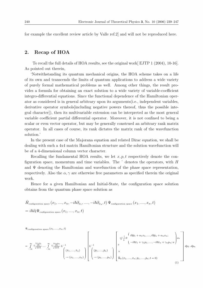
240 Electronic Journal of Theoretical Physics 3, No. 10 (2006) 239–247
for example the excellent review article by Valle ref.2] and will not be reproduced here.
2. Recap of HOA
To recall the full details of HOA results, see the original work[ EJTP 1 (2004), 10-16].
As pointed out therein,
‘Notwithstanding its quantum mechanical origins, the HOA scheme takes on a life
of its own and transcends the limits of quantum applications to address a wide variety
of purely formal mathematical problems as well. Among other things, the result pro-
vides a formula for obtaining an exact solution to a wide variety of variable-coefficient
integro-differential equations. Since the functional dependence of the Hamiltonian oper-
ator as considered is in general arbitrary upon its arguments(i.e., independent variables,
derivative operator symbols[including negative powers thereof, thus the possible inte-
gral character]), then its multivariable extension can be interpreted as the most general
variable coefficient partial differential operator. Moreover, it is not confined to being a
scalar or even vector operator, but may be generally construed an arbitrary rank matrix
operator. In all cases of course, its rank dictates the matrix rank of the wavefunction
solution.’
In the present case of the Majorana equation and related Dirac equation, we shall be
dealing with such a 4x4 matrix Hamiltonian structure and the solution wavefunction will
be of a 4-dimensional column vector character.
Recalling the fundamental HOA results, we let x, p, t respectively denote the con-
figuration space, momentum and time variables. The ˆ denotes the operators, with H
and Ψ denoting the Hamiltonian and wavefunction of the phase space representation,
respectively. Also the α, γ are otherwise free parameters as specified therein the original
work.
Hence for a given Hamiltonian and Initial-State, the configuration space solution
obtains from the quantum phase space solution as
Hconfiguration space (x1, ...., xn,−i�∂x1 , ....,−i�∂xn , t) Ψconfiguration space (x1, ...., xn, t)
= i�∂tΨconfiguration space (x1, ...., xn, t)
Ψconfiguration space (x1, ...., xn, t)
=∞�
−∞e
ix1p12�√4π�
....∞�
−∞e
ixnpn2�√4π�
L−1������
(x1, ...., xn)
→ (x1, ...., xn)
������
��������������
L−1������
(p1, ...., pn)
→ (p1, ...., pn)
������
��������������
e
−i�
t�0
H
������
i�p1 + α1x1, ...., i�pn + αnxn;
−i�x1 + γ1p1, ....,−i�xn + γnpn; u
������
du
�
Ψ0 (x1, ...., xn; p1, ...., pn; t = 0)
��������������
��������������
dp1..dpn
(1)
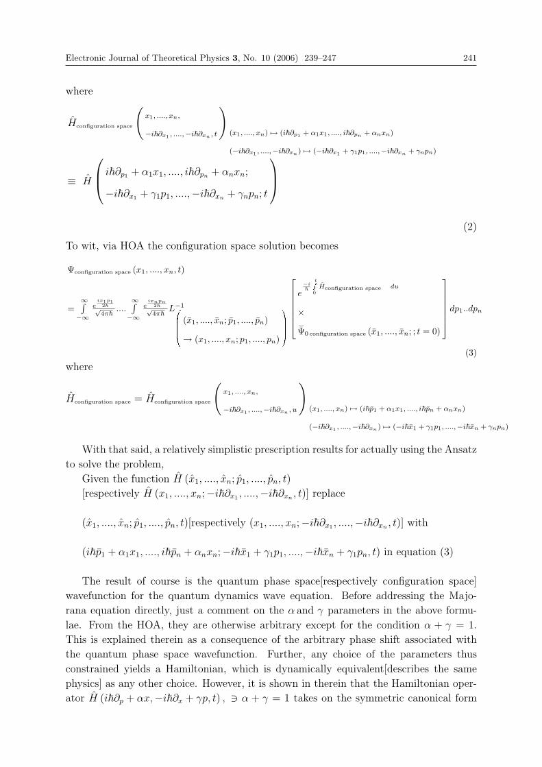
Electronic Journal of Theoretical Physics 3, No. 10 (2006) 239–247 241
where
Hconfiguration space
(x1, ...., xn,
−i�∂x1 , ....,−i�∂xn , t
)(x1, ...., xn) �→ (i�∂p1 + α1x1, ...., i�∂pn + αnxn)
(−i�∂x1 , ....,−i�∂xn ) �→ (−i�∂x1 + γ1p1, ....,−i�∂xn + γnpn)
≡ H
⎛⎜⎝ i�∂p1 + α1x1, ...., i�∂pn + αnxn;
−i�∂x1 + γ1p1, ....,−i�∂xn + γnpn; t
⎞⎟⎠(2)
To wit, via HOA the configuration space solution becomes
Ψconfiguration space (x1, ...., xn, t)
=∞∫
−∞e
ix1p12�√4π�
....∞∫
−∞e
ixnpn2�√4π�
L−1������
(x1, ...., xn; p1, ...., pn)
→ (x1, ...., xn; p1, ...., pn)
������
⎡⎢⎢⎢⎢⎢⎣e
−i�
t�0
Hconfiguration space du
�
Ψ0 configuration space (x1, ...., xn; ; t = 0)
⎤⎥⎥⎥⎥⎥⎦ dp1..dpn
(3)
where
Hconfiguration space = Hconfiguration space
(x1, ...., xn,
−i�∂x1 , ....,−i�∂xn , u
)(x1, ...., xn) �→ (i�p1 + α1x1, ...., i�pn + αnxn)
(−i�∂x1 , ....,−i�∂xn ) �→ (−i�x1 + γ1p1, ....,−i�xn + γnpn)
With that said, a relatively simplistic prescription results for actually using the Ansatz
to solve the problem,
Given the function H (x1, ...., xn; p1, ...., pn, t)
[respectively H (x1, ...., xn;−i�∂x1 , ....,−i�∂xn , t)] replace
(x1, ...., xn; p1, ...., pn, t)[respectively (x1, ...., xn;−i�∂x1 , ....,−i�∂xn , t)] with
(i�p1 + α1x1, ...., i�pn + αnxn;−i�x1 + γ1p1, ....,−i�xn + γ1pn, t) in equation (3)
The result of course is the quantum phase space[respectively configuration space]
wavefunction for the quantum dynamics wave equation. Before addressing the Majo-
rana equation directly, just a comment on the α and γ parameters in the above formu-
lae. From the HOA, they are otherwise arbitrary except for the condition α + γ = 1.
This is explained therein as a consequence of the arbitrary phase shift associated with
the quantum phase space wavefunction. Further, any choice of the parameters thus
constrained yields a Hamiltonian, which is dynamically equivalent[describes the same
physics] as any other choice. However, it is shown in therein that the Hamiltonian oper-
ator H (i�∂p + αx,−i�∂x + γp, t) , $ α + γ = 1 takes on the symmetric canonical form
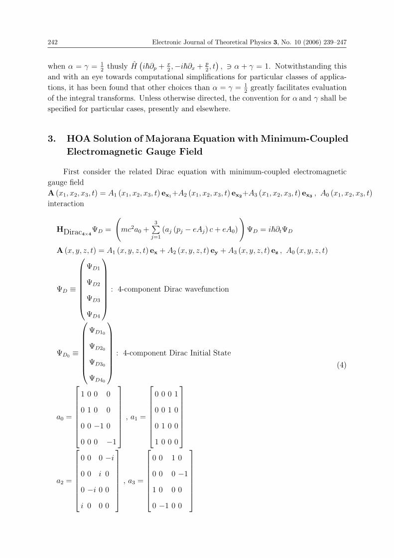
242 Electronic Journal of Theoretical Physics 3, No. 10 (2006) 239–247
when α = γ = 12
thusly H(i�∂p + x
2,−i�∂x + p
2, t), $ α + γ = 1. Notwithstanding this
and with an eye towards computational simplifications for particular classes of applica-
tions, it has been found that other choices than α = γ = 12
greatly facilitates evaluation
of the integral transforms. Unless otherwise directed, the convention for α and γ shall be
specified for particular cases, presently and elsewhere.
3. HOA Solution of Majorana Equation with Minimum-Coupled
Electromagnetic Gauge Field
First consider the related Dirac equation with minimum-coupled electromagnetic
gauge field
A (x1, x2, x3, t) = A1 (x1, x2, x3, t) ex1+A2 (x1, x2, x3, t) ex2+A3 (x1, x2, x3, t) ex3 , A0 (x1, x2, x3, t)
interaction
HDirac4×4ΨD =
(mc2a0 +
3∑j=1
(aj (pj − eAj) c + eA0)
)ΨD = i�∂tΨD
A (x, y, z, t) = A1 (x, y, z, t) ex + A2 (x, y, z, t) ey + A3 (x, y, z, t) ez , A0 (x, y, z, t)
ΨD ≡
⎛⎜⎜⎜⎜⎜⎜⎜⎝
ΨD1
ΨD2
ΨD3
ΨD4
⎞⎟⎟⎟⎟⎟⎟⎟⎠: 4-component Dirac wavefunction
ΨD0 ≡
⎛⎜⎜⎜⎜⎜⎜⎜⎝
ΨD10
ΨD20
ΨD30
ΨD40
⎞⎟⎟⎟⎟⎟⎟⎟⎠: 4-component Dirac Initial State
a0 =
⎡⎢⎢⎢⎢⎢⎢⎢⎣
1 0 0 0
0 1 0 0
0 0 −1 0
0 0 0 −1
⎤⎥⎥⎥⎥⎥⎥⎥⎦, a1 =
⎡⎢⎢⎢⎢⎢⎢⎢⎣
0 0 0 1
0 0 1 0
0 1 0 0
1 0 0 0
⎤⎥⎥⎥⎥⎥⎥⎥⎦
a2 =
⎡⎢⎢⎢⎢⎢⎢⎢⎣
0 0 0 −i
0 0 i 0
0 −i 0 0
i 0 0 0
⎤⎥⎥⎥⎥⎥⎥⎥⎦, a3 =
⎡⎢⎢⎢⎢⎢⎢⎢⎣
0 0 1 0
0 0 0 −1
1 0 0 0
0 −1 0 0
⎤⎥⎥⎥⎥⎥⎥⎥⎦
(4)
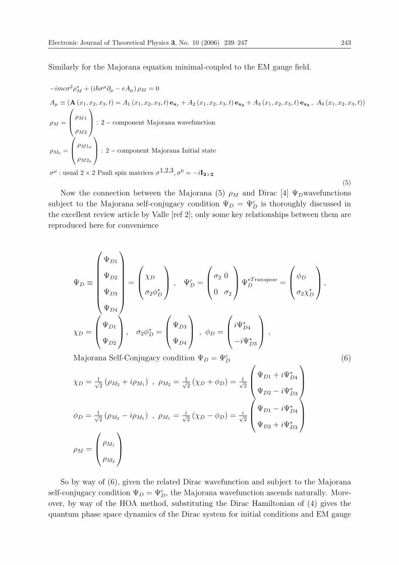
Electronic Journal of Theoretical Physics 3, No. 10 (2006) 239–247 243
Similarly for the Majorana equation minimal-coupled to the EM gauge field.
−imcσ2ρ∗M + (i�σμ∂μ − eAμ) ρM = 0
Aμ ≡ (A (x1, x2, x3, t) = A1 (x1, x2, x3, t) ex1 + A2 (x1, x2, x3, t) ex2 + A3 (x1, x2, x3, t) ex3 , A0 (x1, x2, x3, t))
ρM =
⎛⎜⎝ ρM1
ρM2
⎞⎟⎠ : 2− component Majorana wavefunction
ρM0 =
⎛⎜⎝ ρM10
ρM20
⎞⎟⎠ : 2− component Majorana Initial state
σμ : usual 2× 2 Pauli spin matrices σ1,2,3, σ0 = −iI2×2
(5)
Now the connection between the Majorana (5) ρM and Dirac [4] ΨDwavefunctions
subject to the Majorana self-conjugacy condition ΨD = ΨcD is thoroughly discussed in
the excellent review article by Valle [ref 2]; only some key relationships between them are
reproduced here for convenience
ΨD ≡
⎛⎜⎜⎜⎜⎜⎜⎜⎝
ΨD1
ΨD2
ΨD3
ΨD4
⎞⎟⎟⎟⎟⎟⎟⎟⎠=
⎛⎜⎝χD
σ2φ∗D
⎞⎟⎠ , ΨcD =
⎛⎜⎝σ2 0
0 σ2
⎞⎟⎠Ψ∗TransposeD =
⎛⎜⎝φD
σ2χ∗D
⎞⎟⎠ ,
χD =
⎛⎜⎝ΨD1
ΨD2
⎞⎟⎠ , σ2φ∗D =
⎛⎜⎝ΨD3
ΨD4
⎞⎟⎠ , φD =
⎛⎜⎝ iΨ∗D4
−iΨ∗D3
⎞⎟⎠ ,
Majorana Self-Conjugacy condition ΨD = ΨcD
χD = 1√2(ρM2 + iρM1) , ρM2 = 1√
2(χD + φD) = 1√
2
⎛⎜⎝ΨD1 + iΨ∗D4
ΨD2 − iΨ∗D3
⎞⎟⎠φD = 1√
2(ρM2 − iρM1) , ρM1 = i√
2(χD − φD) = i√
2
⎛⎜⎝ΨD1 − iΨ∗D4
ΨD2 + iΨ∗D3
⎞⎟⎠ρM =
⎛⎜⎝ ρM1
ρM2
⎞⎟⎠
(6)
So by way of (6), given the related Dirac wavefunction and subject to the Majorana
self-conjugacy condition ΨD = ΨcD, the Majorana wavefunction ascends naturally. More-
over, by way of the HOA method, substituting the Dirac Hamiltonian of (4) gives the
quantum phase space dynamics of the Dirac system for initial conditions and EM gauge
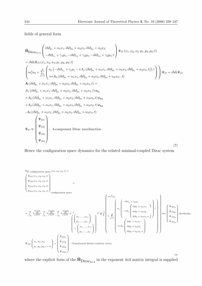
244 Electronic Journal of Theoretical Physics 3, No. 10 (2006) 239–247
fields of general form.
HDirac4×4
⎛⎜⎝ i�∂p1 + α1x1, i�∂p2 + α2x2, i�∂p3 + α3x3;
−i�∂x1 + γ1p1,−i�∂x2 + γ2p2,−i�∂x3 + γ3p3; t
⎞⎟⎠ΨD (x1, x2, x3; p1, p2, p3; t)
= i�∂tΨD (x1, x2, x3; p1, p2, p3; t)⎛⎜⎝m2ca0 +
3∑j=1
⎛⎜⎝ aj
(−i�∂xj+ γjpj − eAj (i�∂p1 + α1x1, i�∂p2 + α2x2, i�∂p3 + α3x3, t)
)c
+eA0 (i�∂p1 + α1x1, i�∂p2 + α2x2, i�∂p3 + α3x3; , t)
⎞⎟⎠⎞⎟⎠ΨD = i�∂tΨD
A (i�∂p1 + α1x1, i�∂p2 + α2x2, i�∂p3 + α3x3, t) =
A1 (i�∂p1 + α1x1, i�∂p2 + α2x2, i�∂p3 + α3x3, t) ex1
+A2 (i�∂p1 + α1x1, i�∂p2 + α2x2, i�∂p3 + α3x3, t) ex2
+A3 (i�∂p1 + α1x1, i�∂p2 + α2x2, i�∂p3 + α3x3, t) ex3
, A0 (i�∂p1 + α1x1, i�∂p2 + α2x2, i�∂p3 + α3x3, t)
ΨD ≡
⎛⎜⎜⎜⎜⎜⎜⎜⎜⎝
ΨD1
ΨD2
ΨD3
ΨD4
⎞⎟⎟⎟⎟⎟⎟⎟⎟⎠: 4-component Dirac wavefunction
(7)
Hence the configuration space dynamics for the related minimal-coupled Dirac system
ΨD configuration space (x1, x2, x3, t) =�����������
ΨD1 (x1, x2, x3, t)
ΨD2 (x1, x2, x3, t)
ΨD3 (x1, x2, x3, t)
ΨD4 (x1, x2, x3, t)
�����������
configuration space
=
=∞�
−∞e
ix1p12�√4π�
∞�−∞
e
ix2p22�√4π�
∞�−∞
e
ix3p32�√4π�
L−1��������������
����
x1, ...., xn;
p1, ...., pn
����
→
����
x1, ...., xn;
p1, ...., pn
����
��������������
e( −i�
t�0
����������������������������
mc2a0
+3�
j=1
������������������������
aj
�����������
−i�xj + γjpj
−eAj
��������
i�p1 + α1x1,
i�p2 + α2x2,
i�p3 + α3x3, u
��������
�����������
c
+eA0
��������
i�p1 + α1x1,
i�p2 + α2x2,
i�p3 + α3x3, u
��������
������������������������
����������������������������
du)
�����������
�ΨD01�ΨD02�ΨD03�ΨD04
�����������
dp1dp2dp3
�ΨD0
����
x1, x2, x3;
p1, p2, p3; t = 0
���� =
�����������
�ΨD01�ΨD02�ΨD03�ΨD04
�����������
: Transformed Initial-condition vector
(8)
where the explicit form of the HDirac4×4in the exponent 4x4 matrix integral is supplied
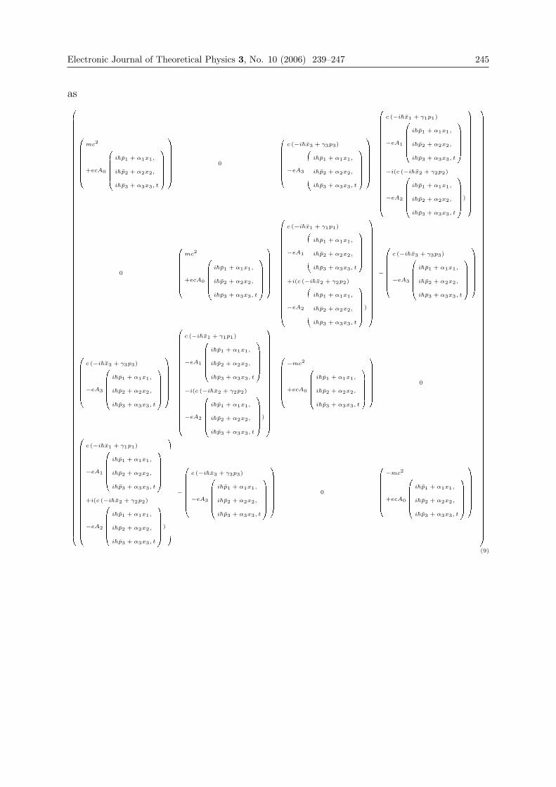
Electronic Journal of Theoretical Physics 3, No. 10 (2006) 239–247 245
as������������������������������������������������������������������������������������������������������������������������������
�����������
mc2
+ecA0
��������
i�p1 + α1x1,
i�p2 + α2x2,
i�p3 + α3x3, t
��������
�����������
0
�����������
c (−i�x3 + γ3p3)
−eA3
��������
i�p1 + α1x1,
i�p2 + α2x2,
i�p3 + α3x3, t
��������
�����������
����������������������������
c (−i�x1 + γ1p1)
−eA1
��������
i�p1 + α1x1,
i�p2 + α2x2,
i�p3 + α3x3, t
��������
−i(c (−i�x2 + γ2p2)
−eA2
��������
i�p1 + α1x1,
i�p2 + α2x2,
i�p3 + α3x3, t
��������
)
����������������������������
0
�����������
mc2
+ecA0
��������
i�p1 + α1x1,
i�p2 + α2x2,
i�p3 + α3x3, t
��������
�����������
����������������������������
c (−i�x1 + γ1p1)
−eA1
��������
i�p1 + α1x1,
i�p2 + α2x2,
i�p3 + α3x3, t
��������
+i(c (−i�x2 + γ2p2)
−eA2
��������
i�p1 + α1x1,
i�p2 + α2x2,
i�p3 + α3x3, t
��������
)
����������������������������
−
�����������
c (−i�x3 + γ3p3)
−eA3
��������
i�p1 + α1x1,
i�p2 + α2x2,
i�p3 + α3x3, t
��������
�����������
�����������
c (−i�x3 + γ3p3)
−eA3
��������
i�p1 + α1x1,
i�p2 + α2x2,
i�p3 + α3x3, t
��������
�����������
����������������������������
c (−i�x1 + γ1p1)
−eA1
��������
i�p1 + α1x1,
i�p2 + α2x2,
i�p3 + α3x3, t
��������
−i(c (−i�x2 + γ2p2)
−eA2
��������
i�p1 + α1x1,
i�p2 + α2x2,
i�p3 + α3x3, t
��������
)
����������������������������
�����������
−mc2
+ecA0
��������
i�p1 + α1x1,
i�p2 + α2x2,
i�p3 + α3x3, t
��������
�����������
0
����������������������������
c (−i�x1 + γ1p1)
−eA1
��������
i�p1 + α1x1,
i�p2 + α2x2,
i�p3 + α3x3, t
��������
+i(c (−i�x2 + γ2p2)
−eA2
��������
i�p1 + α1x1,
i�p2 + α2x2,
i�p3 + α3x3, t
��������
)
����������������������������
−
�����������
c (−i�x3 + γ3p3)
−eA3
��������
i�p1 + α1x1,
i�p2 + α2x2,
i�p3 + α3x3, t
��������
�����������
0
�����������
−mc2
+ecA0
��������
i�p1 + α1x1,
i�p2 + α2x2,
i�p3 + α3x3, t
��������
�����������
������������������������������������������������������������������������������������������������������������������������������
(9)
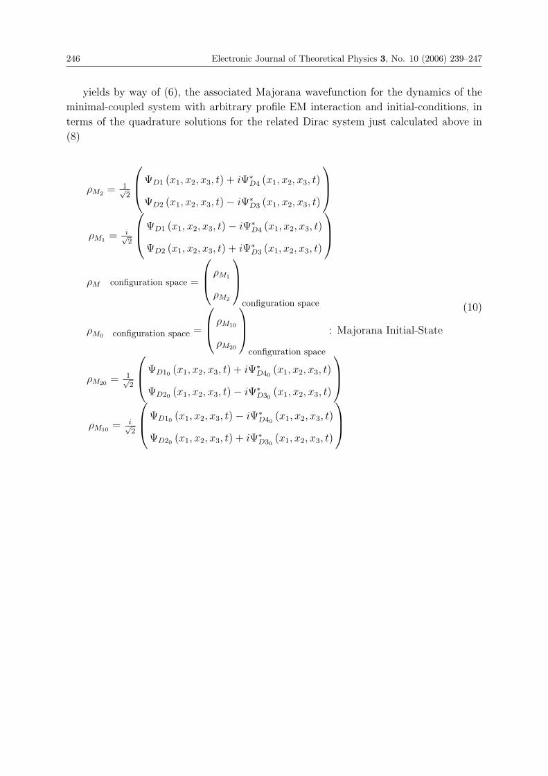
246 Electronic Journal of Theoretical Physics 3, No. 10 (2006) 239–247
yields by way of (6), the associated Majorana wavefunction for the dynamics of the
minimal-coupled system with arbitrary profile EM interaction and initial-conditions, in
terms of the quadrature solutions for the related Dirac system just calculated above in
(8)
ρM2 = 1√2
⎛⎜⎝ΨD1 (x1, x2, x3, t) + iΨ∗D4 (x1, x2, x3, t)
ΨD2 (x1, x2, x3, t)− iΨ∗D3 (x1, x2, x3, t)
⎞⎟⎠ρM1 = i√
2
⎛⎜⎝ΨD1 (x1, x2, x3, t)− iΨ∗D4 (x1, x2, x3, t)
ΨD2 (x1, x2, x3, t) + iΨ∗D3 (x1, x2, x3, t)
⎞⎟⎠ρM configuration space =
⎛⎜⎝ ρM1
ρM2
⎞⎟⎠configuration space
ρM0 configuration space =
⎛⎜⎝ ρM10
ρM20
⎞⎟⎠configuration space
: Majorana Initial-State
ρM20 = 1√2
⎛⎜⎝ΨD10 (x1, x2, x3, t) + iΨ∗D40
(x1, x2, x3, t)
ΨD20 (x1, x2, x3, t)− iΨ∗D30
(x1, x2, x3, t)
⎞⎟⎠ρM10 = i√
2
⎛⎜⎝ΨD10 (x1, x2, x3, t)− iΨ∗D40
(x1, x2, x3, t)
ΨD20 (x1, x2, x3, t) + iΨ∗D30
(x1, x2, x3, t)
⎞⎟⎠
(10)

Electronic Journal of Theoretical Physics 3, No. 10 (2006) 239–247 247
References
[1] E. Majorana, Nuovo Cimento 9, P335 (1932)
[2] J.W.F.Valle, Prog.Part.Nucl.Phys.26,pp91-171 (1991)
EJTP 3, No. 10 (2006) 249–263 Electronic Journal of Theoretical Physics
A Logical Analysis of Majorana’s Papers ofTheoretical Physics
A. Drago 1 ∗ and S. Esposito 2 †
1Universita di Pisa, Pisa, Italy2Universita di Napoli “Federico II” ,Naples, Italy
Received 28 April 2006, Published 28 May 2006
Abstract: We study two celebrated Majorana’s papers through a method of investigationwhich relies upon the recently recognised distinction between classical logic and grosso modothe several kinds of non-classical logics, i.e. the failure of the double negation law. This lawfails when a double negated sentence is not equivalent to the corresponding positive sentence,owing to the lack of scientific evidence of the latter one. All recognised double negated sentencesinside the text of each paper are listed; the mere sequence of such sentences gives the logicalthread of Majorana’s arguing. This one is recognised to be of the Lagrangian kind, which mixeslogical arguing and mathematical calculation; i.e. the author puts a fundamental problem whichis solved by anticipating the mathematical hypothesis which is capable of solving it, and thenby drawing from this hypothesis the mathematical consequences in order to obtain the desiredresult. Furthermore Majorana’s rhetoric of presentation results to be a juridical one, owing tohis style of presenting the laws to which an ideal theoretical physicist has to conform himself inorder to solve the problem at issue.c© Electronic Journal of Theoretical Physics. All rights reserved.
Keywords: Ettore Majorana, Logical AnalysisPACS (2006): 01.65.+g,01.30.Tt,02.10.-v
1. Introduction
Recently the interest for the human and scientific figure of Ettore Majorana acquired
vigour. Apart several biographies and books (about his life and in particular about the
unsolved problem of his disappearance [1]), the following books have been edited: the
last lectures at Naples University in Italian language [2]; and, in English language, his
”Volumetti” [3], where Majorana was accustomed to solve for his own interest scientific
250 Electronic Journal of Theoretical Physics 3, No. 10 (2006) 249–263
problems of various kinds; it seems that his accuracy and precision was the higher one
with respect to any other scientist’s notebook. This element supports what Fermi spoke
about him:
“. . . in the world there are various categories of scientists: people of a secondary or
tertiary standing, who do their best but do not go very far. There are also those of high
standing, who come to discoveries of great importance, fundamental for the development
of science’ (and here I had the impression that he placed himself in that category). ‘But
then there are geniuses like Galileo and Newton. Well, Ettore was one of them. Majorana
had what no one else in the world had . . . ” [4].
Maybe such an evaluation appears somewhat apologetic; but Fermi saw some other
elements. In the following we want to analyse a characteristic feature of Majorana papers
- i.e. the kind of logic in his arguments - which was missed in previous analysis.
2. Majorana as a Theoretical Physicist: Papers and Publica-
tions
The scientific production by E. Majorana includes nine printed publications [5]. In
last years some studies wanted to put such papers inside a historical background, then
to interpret them and possibly to develop them for achieving new results.
Some decades ago E. Amaldi wrote a review on Majorana’s scientific production [6];
he first offered a detailed valuations of them; it constitutes a first characterisation of
Majorana’s work in theoretical physics.
Furthermore in last years some improvements have been considered of the ideas that
Majorana started to develop and then have been forgotten - though independently recu-
perated by others -; in particular, his solutions of those differential equations which are
useful in many physical problems [7].A first valuation for Majorana’s work on symme-
tries has been given; along with Giovanni Gentile jr, for the first time he introduced this
mathematical tool in the Italian theoretical physics scenario [8]. It is also interesting to
note that he was almost the unique (though remote) Weyl’s follower in Weyl’s attitude
of founding quantum mechanics and the field theory through group theory only [9].
The problem is open whether it is possible to reconstruct Majorana’s scientific pro-
duction according to a line of development which represents a conception of theoretical
physics as a whole, for instance a conception similar to H. Weyl’s.
The present paper is aimed to improve the comprehension of Majorana’s papers by
means of a technique of mathematical logic. Among his papers we have chosen two of
the most important papers in theoretical physics: Teoria relativistica di particelle con
momento intrinseco arbitrario (Relativistic theory of particles with arbitrary intrinsic
momentum) of 1932 and Teoria simmetrica dell’elettrone e del positrone (Symmetric
theory of electron and positron) of 1937 [10]. The historical background of these papers
is offered by the above mentioned Amaldi’s review.
Electronic Journal of Theoretical Physics 3, No. 10 (2006) 249–263 251
3. Analysis of a Scientific Writing by Means of Non-Classical
Logic
In the above-mentioned text Majorana illustrates a theory which is based upon a
very general problem, i.e. the relativistic generalisation of Dirac theory of the electron for
particles of arbitrary spin. For solving this problem, a deductive method of solution does
not a priori exist. The final result is not deductively drawn from some a priori principle;
rather, the arguments proceed in a heuristic way, without absolute certainty.
Elsewhere, one of us (A. D.) suggested the model of theoretical organisation aimed
to search a new scientific method capable to solve a given universal problem [11]. Inside
this kind of organisation, called a problem-based one, several double negated sentences
(DNS) play a crucial role, each one being not equivalent to the corresponding positive
sentence, owing to the lack of (either experimental or theoretical) scientific evidence of
the latter one. For instance, in the historical development of thermodynamics very often
the following sentence occurs: ”It is impossible the perpetual (= without an end) motion”
(we underlined the negations for evidentiating them to the reader; the same will be done
in the following DNSs); the corresponding positive statement is ”Each motion has an
end”; in order to state it we have to know either the instant or the place where the
given motion will end; this knowledge is impossible, owing to our ignorance of both the
friction function which affects the motion and the length of the path along which friction
is exerted upon the body in motion. Hence, the positive sentence is not supported by
scientific facts.
In 20th Century the studies upon the foundations of mathematical logic resulted in
establishing more precisely the borderline between classical logic and grosso modo non-
classical logics; this bordeline is the failure of rather than the law of excluded middle
(either A or not-A), the double negation law (not-not-A =A) [12]. This change in the
attention is very relevant for, since inside a scientific writing a scholar easily recognises a
sentence not-not-A and then easily he tests whether in this sentence the double negation
logical law holds true or not, by testing whether the corresponding sentence A is supported
by scientific evidence or not.
According to what occurs in the problem-based theories, in Majorana’s paper too
occur DNSs; hence, Majorana was surely out of a full deductive theory in classical logic.
Hence, it is useful to analyse his writings under this logical aspect. To this aim it is
necessary first to list all DNSs included by Majorana’s paper.
4. Inspection of All DNSs in Teoria Relativistica (1932)
Let us analyse the paper by recognising the DNSs inside it. In order to make easier
the reader to recognise the DNS nature of each sentence listed in the following, the
corresponding positive sentence is written inside square brackets, after a sign �=.
There exists several kinds of DNSs. Beyond the plain DNSs (either a sentence or a
word including two negations say, in-variant, etc.) there are the ”weak” DNSs (in the
252 Electronic Journal of Theoretical Physics 3, No. 10 (2006) 249–263
following: wDNS), that is those including a modality, as ”may”, ”allow”, ”want”, ”must”
(in the following each of these words is written in Italic and the order number of its
DNS is marked by an asterisk*). The appearance of these words is quite improper in a
scientific text, meant in a traditional sense, i.e. as a deductive exposition; because this
exposition has to be based upon either experimental or deductive certainties; if instead
such modalities occur, they show that the arguing is heuristic in nature; in such a case
they have to be expressed by means of DNSs; for ex. ”may = it is not true that it is
not”.
Furthermore, by taking into account that Majorana ignored at all non-classical logic,
we will consider as a DNS also sentences which are DNS in a more general sense, for
example the words ”equivalent”, ”analogous”, similar, each one to be meant as ”not
unequal”.
1*. (p. 335) [...] A relativistic generalisation of the previous theory must [= it is
not true that is not] satisfy [ �= satisfies] to the following conditions when its degree of
accuracy is growing up:
2*. (a) The theory allows the study of [ �= studies] particles having velocity almost
determined in magnitude and direction,...
3. ... giving results which are equivalent [= that are not different from] [�= equal] to
the non relativistic theory,...
4. (p. 336) without however the necessity of choosing [= differentiate] a particular
reference system [ �= for all systems].
5*. (b) The theory moreover allows to study [ �= studies] processes where the velocities
of the particles vary slowly, but in an extended range, owing to weak external fields.
6. (c) The theory is valid in general, whatever be undetermined [ �= for an arbitrary
determination of] the velocity of the particles.
7. [...] On the contrary, it is likely [= it is not true that it is not] [ �= is true] that...
8. ... a theory satisfying (b) and only in part (c) does not hurt in subtantial difficulties
[�= is valid].. .
9*. ... its physical content can be [= it is not true that it is not] [ �= is] essentially
the same justifying the Schroedinger equation.
10. The most remarkable example of such generalisations is just offered by dirac’s
theory, but since this applies only to particles with intrinsic momentum s=1/2, I looked
for analogous [= not different] [ �= equal] in form equations to dirac’s, though somewhat
more cumbersome,...
11*. ... which allow to consider [ �= consider] particles with arbitrary momentum, also
for a vanishing value of it
12*. [...] Equations of this kind [that is Dirac-like] present a difficulty of principle.
The operator -1 indeed must transform [�=transforms] as the temporal component of a
4-vector...
13*. ... and so β cannot be [�= is] merely a multiple of the unity matrix,...
14*. ... but must have [�= has] at least two different eigenvalues, say β1 and β2 ;...
15*. ... but from this fact follows that the rest-energy of the particles, which is
Electronic Journal of Theoretical Physics 3, No. 10 (2006) 249–263 253
obtained from the (1) by putting p = 0, must have [�= has] at least two different values,
β1mc2 and β2mc2.
16*. According to the dirac equation the possible values of the rest mass are, as
it is well-known, +m and -m, from which, due to the relativistic invariance follows that
the energy can have [�= has] two different values owing to the sign of each value of p :
W = ±√m2c4 + c2p2.
17. The indeterminacy in the sign of energy can be overcame [= cancelled] [ �=is
determined], by using equations of the fundamental kind (1),...
18. (p. 337) ... only if the wave function has infinite components which not [Italic
in the text] allow to be broken [= not-reducible] [ �= elementary] in finite tensors or finite
spinors.
19*. 1. The equation (1) can be [�= is] deduced from the variational principle [a
formula follows].
20. One of the conditions of relativistic in-variance [�= constancy]...
21. ... has of course to be in-variant [�= constant] the form [a formula follows].
22*. If now we want that the rest-energy result [ �= when the rest-energy is] always
positive,...
23*. ... the eigenvalues of β must be [�= are] all positive ones and the form [a formula
follows] will be positive definite.
24*. Then it is possible to reduce [ �= reduces] through a non-unitary transformation
ψ → ϕ such a form to the unity form: [a formula follows].
25. By substituting in (2) for ψ his expression by means of ϕ one will have: [a formula
follows] from which the equations equivalent [�= egual] to (1) follow: [a formula follow].
26*. We now must determine the law of transformation of ϕ according to a lorentz
rotation and moreover expression of matrices...
27. ... in such a way that the relativistic in-variance [�= constancy] of the variational
principle be satisfied (4)...
28. ... and hence the function to be integrated be invariant [�= constant].
29*. Let us start by stating the law of transformation of ϕ by observing first of all
that the invariance of [a formula follow] means that we must consider [�= we consider]
unitary transformations only.
30*. (p. 338) The operators a e b must be [�= are] Hermitian in a unitary representation
and viceversa;...
31*. ... furthermore, in order to the infinitesimal transformations to be integrable
must satisfy [�= satisfy] some commutation relations which are deduced from both (6)
and (7): (formulas follow) and the orther ones which are obtained by permutation of x,
y and z.
32. (p. 339) The denomination ” zero-index ” means that is zero the in-variant [=
the constant operator]: [a formula follows].
33*. [...] 2. We now must determine [ �= we determine] the operators [a formula
follows]...
34. ... in such a way that (4) be invariant [�= constant].
254 Electronic Journal of Theoretical Physics 3, No. 10 (2006) 249–263
35*. Because we consider unitary transformations only, the above-mentioned opera-
tors transform as the Hermitian forms related to them, and hence owing to the invariance
[�= constancy] of the integrand function in (4)...
36. ... it is necessary that they constitute [�= constitute] a covariant vector [a formula
follows].
37*. [...] The operators γ must satisfy [�= satisfy] the exchange relations [formulas
follow] and some others obtained by cyclical permutation of x, y, z.
38. (p. 342) [...] Without difficulties [�= easily] it is verified that...
39*. [...] These states can be regarded [�= are] as belonging to the imaginary value ik
of the mass.
40*. We now want to consider [�= consider] quickly the introduction of the electro-
magnetic field in equation (16).
41. (p. 343) For instance we may add invariant [�= constant] terms,...
42. ... analogous [�= equal] to those introduced by Pauli in the theory of the magnetic
neutron, which considers the field strength instead of the electromagnetic potentials,...
43. ... so that to do not unsettle [ �= maintain as a constant]...
44. ... the invariance [�= the constancy] of the equations according to the indetermi-
nacy of the potentials.
In total, in 10 pages of this paper we recognised 21 DNSs (among them 6 are due to
the word ”invariant”) and 23 wDNSs.
5. Analysis of the Arguing in Teoria Relativistica(1932)
The same kind of analysis when applied to scientific texts written by some other
authors, gives each time a list of DNSs, whose sequence is sufficient to manifest the
logical thread of the presentation at issue. This is the case for instance of the discursive
part of S. Carnot’s booklet, i.e. the part originating most of modern thermodynamics. His
theory is a problem-based theory since it puts a universal problem: whether a maximum
efficiency in converting heat into work there exists.
Its sequence of DNSs can be broken into some units of arguing; each unit starts
from a DNS setting a problem, then some DNSs establish methodological principles
leading to construct a result which, in a rigorous way, is obtained by means of an ad
absurdum argument, such as it is the celebrated S. Carnot’s theorem in thermodynamics
[13]. But this is not the case of Majorana’s paper, because the DNSs are intermixed with
mathematical derivations; where each mathematical formula includes an exact equality;
hence, the negation of the negation of the formula gives again the same formula, in
agreement with classical logic and contrarily to the case of a DNS.
However, a more sophisticated case than S. Carnot’s thermodynamics is given by La-
grange’s mechanics. This theory too wanted to solve a great problem, which Lagrange
himself stated, i.e., how to develop a theory of mechanical phenomena including con-
straints. Also inside Lagrange’s book (Mecanique analytique) we recognise DNSs; it is
even possible to point out some units of arguing; each one of them starting from a new
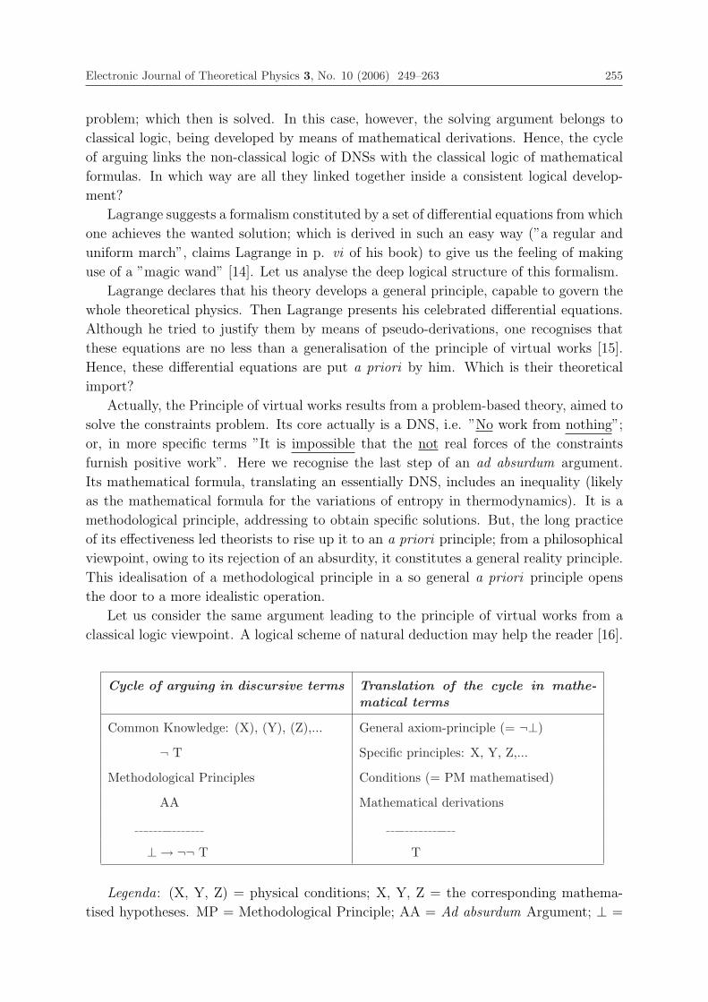
Electronic Journal of Theoretical Physics 3, No. 10 (2006) 249–263 255
problem; which then is solved. In this case, however, the solving argument belongs to
classical logic, being developed by means of mathematical derivations. Hence, the cycle
of arguing links the non-classical logic of DNSs with the classical logic of mathematical
formulas. In which way are all they linked together inside a consistent logical develop-
ment?
Lagrange suggests a formalism constituted by a set of differential equations from which
one achieves the wanted solution; which is derived in such an easy way (”a regular and
uniform march”, claims Lagrange in p. vi of his book) to give us the feeling of making
use of a ”magic wand” [14]. Let us analyse the deep logical structure of this formalism.
Lagrange declares that his theory develops a general principle, capable to govern the
whole theoretical physics. Then Lagrange presents his celebrated differential equations.
Although he tried to justify them by means of pseudo-derivations, one recognises that
these equations are no less than a generalisation of the principle of virtual works [15].
Hence, these differential equations are put a priori by him. Which is their theoretical
import?
Actually, the Principle of virtual works results from a problem-based theory, aimed to
solve the constraints problem. Its core actually is a DNS, i.e. ”No work from nothing”;
or, in more specific terms ”It is impossible that the not real forces of the constraints
furnish positive work”. Here we recognise the last step of an ad absurdum argument.
Its mathematical formula, translating an essentially DNS, includes an inequality (likely
as the mathematical formula for the variations of entropy in thermodynamics). It is a
methodological principle, addressing to obtain specific solutions. But, the long practice
of its effectiveness led theorists to rise up it to an a priori principle; from a philosophical
viewpoint, owing to its rejection of an absurdity, it constitutes a general reality principle.
This idealisation of a methodological principle in a so general a priori principle opens
the door to a more idealistic operation.
Let us consider the same argument leading to the principle of virtual works from a
classical logic viewpoint. A logical scheme of natural deduction may help the reader [16].
Cycle of arguing in discursive terms Translation of the cycle in mathe-
matical terms
Common Knowledge: (X), (Y), (Z),... General axiom-principle (= ¬⊥)
¬ T Specific principles: X, Y, Z,...
Methodological Principles Conditions (= PM mathematised)
AA Mathematical derivations
⊥ → ¬¬ T T
Legenda: (X, Y, Z) = physical conditions; X, Y, Z = the corresponding mathema-
tised hypotheses. MP = Methodological Principle; AA = Ad absurdum Argument; ⊥ =
256 Electronic Journal of Theoretical Physics 3, No. 10 (2006) 249–263
Absurd. To draw consequences is represented by the vertical line.
Notice that whereas the first column shows the (non-classical) implication ¬ T → ⊥,
the second column shows the classical converse of this implication (let us recall that if
M → N, the classical converse (which yet is rejected by non-classical logic) is ¬ N → ¬M), i.e. ¬⊥ → ¬¬ T → T ; just what classical logic allows, i.e. to reverse through
a conversion laws an ad absurdum argument in an affirmative argument, however the
conclusion may be idealistic in nature.
Let us reverse the path of the previous argument leading to the methodological prin-
ciple of the virtual works, so to start from its final step; then the negated absurdum is
equivalent a positive sentence. Which by a mathematical step, can be referred no more to
the constraints reactions, but to the resulting active forces; then it, by concerning these
forces which can be a posteriori experimented, seems a full physical principle. Hence,
its philosophical nature of a reality principle together with the (semi-)physical nature of
its mathematical formula qualify it as an instance of theoretical omniscience (”all the
necessary equations for the solution of each problem”, p. 12).
When it is applied no more to forces, but, through the Lagrange’s celebrated step
Σ(fi-ma i)=0, to velocities it becomes an omniscient principle on dynamical equilibria.
In total, Lagrange generalises the negated absurdum to a very general mathematical
formula, playing the role of an omniscient principle.
However, the nature of the theory to be a problem-based one, is not lost. The last step,
the solution of the problem at issue, is obtained not in forces causing effects (trajectories),
but in in-variants (about energy, momentum, etc.), i.e. the same results originated by
each theory based upon a general problem.
Majorana’s paper, though including DNSs, does not conform to Carnot’s problem-
atic model but to Lagrange’s; indeed, ad absurdum arguments are absent. In order to
solve the problem at issue he introduces a sophisticated formalism (variational calculus
applied upon the action principle, theory of group representations), which in fact is the
Lagrangian formalism. Then, he develops the arguments in a full mathematical way; once
he recognises the suitable hypotheses (which actually suggest the restrictions under which
the problem is solvable) he puts them as mathematical premises; then the subsequent
development merely verify that they effectively solve the problem at issue. We conclude
that his arguing is similar to Lagrange’s.
6. The Scheme of Arguing in Teoria Relativistica (1932)
From both the direct reading of the paper (without taking in account DNSs) and by
the knowledge of the scientific subject dealt with, one recognises the following thread of
the speech.
[General problem] (p. 335) To generalise Schroedinger’s mechanics to the relativistic
framework
The generalisation has to satisfy three conditions: (a), (b) e (c) [see DNSs no.s 2, 5
and 6]
Electronic Journal of Theoretical Physics 3, No. 10 (2006) 249–263 257
The third condition is not easy to be satisfied
Dirac equation has already solved the problem under the conditions (b) and in part
(c)
But Dirac equation holds only for spin s = 1/2 .
[Specific problem] (p. 336) A generalisation is required for arbitrary spin
In Dirac equation the mass operator assumes two eigenvalues, a positive and a negative
one
[Methodological principle: it seems an unnatural fact the negative mass or, equiva-
lently (in the theory of relativity), negative energy]
[Methodological principle] (p. 336) Looking for an equation which is similar to Dirac’s,
but dealing with only positive mass.
[Anticipation of the solution in a mathematical form] (pp. 336-337) The equation can
be obtained by introducing a condition upon the wave function: this has an infinite num-
ber of components forming an irreducible representation of the Lorentz group; Majorana
thus makes use of unitary infinite-dimensional representations of the Lorentz group.
[Having apperceived by intuition the possible final solution, the development comes
back to the problem and a mathematical step is performed ] (p. 337) In order to go from
the wave function pertaining to Dirac equation to that pertaining to the novel equation
to be recognised, a non-unitary transformation is required.
[Position of the principle of mathematical omnisolution from which to draw the desired
solution] (p. 337) Variational principle on the action function.
From this principle Dirac equation can be obtained.
In Dirac equation the operator β m cˆ2 [=β m c2] is the only one including the mass;
it is an invariant.
[Anticipation of the mathematical solution] (p. 337) In order to obtain only positive
mass values, it is necessary that the matrix β has only positive eigenvalues.
[Methodological principle] (p. 337) This can be achieved by changing the β operator
by means of a non-unitary transformation.
[Result ] (p. 337) The general form of the Majorana equations are obtained, as a
modification of the Dirac’s one.
[Subordinate Problem] The subsequent task is to establish the invariance of the wave
function under the Lorentz group, being the matrices γ occurring in the Majorana equa-
tion undefined.
[Methodological principle] (p. 337) An infinitesimal Lorentz transformation does it.
A Hermitian infinite-dimensional representation of the above group is considered.
[Result ] (p. 339) Infinite spinors and tensors.
[Subordinate Problem] (p. 339) Majorana looks for the invariance of γ matrices
[Methodological principle] under the Lorentz group; he obtains an explicit expression
for them.
[General result ] (p. 342) Hence, the obtained infinite-dimensional representations of
the γ’s gives the complete determination of his equations.
[Further problem] (p. 342) Generalisation in order to include electromagnetic inter-
258 Electronic Journal of Theoretical Physics 3, No. 10 (2006) 249–263
action.
[Methodological principle, chosen among various other methodological principles ] (p.
343) A transformation on both W and p introducing electric charge, scalar and potential
vectors; the new equations are obtained and discussed.
Let us now come back to the list of DNS.
The interpretative analysis of the paper in units of non-classical logic arguing, ex-
pressed by DNSs, is as follows:
1˚ unit : The DNSs 1-11 describe the theoretical background; the general problem is
put by (DNS 1,10). This unit will be closed by means of the 4˚unit.
2˚ unit : The specific problem of eliminating negative values of mass is expressed
(DNSs 12-16); some methodological principles for solving it follow, i.e. the use of Dirac-
like equation, variational principle (DNSs 17-19) and Lorentz invariance of the equation
(DNSs 20-21); the problem is then reiterated (DNS 22), the condition for the invariance of
the coefficients is introduced in a mathematised form (DNS 24) and the result (Majorana
equations) is obtained (DNS 25).
3˚ unit : The problem of the transformation law of the wave function ϕ is put (DNSs
26-28) and after the methodological principle of unitarian representations (DNS 29), the
result is obtained (DNS 30-32).
4˚ unit : After both the problem of determining the operators for the Lorentz invari-
ance of the equations (DNSs 33-34), and the methodological principle (DNS 35-36), the
result is obtained and discussed (DNS 37-38)
5˚ unit : After the problem (DNS 40), he chooses among many others a method-
ological principle for introducing electromagnetic fields in analogy to Pauli theory in the
magnetic neutron (DNSs 41-44).
In total, we have five units of arguing; but they are not cycles of arguing, because,
by relying the arguing upon mathematical deduction, it never ends by means of an ad
absurdum theorem; i.e. that kind of arguing which has to close a correct arguing in
non-classical logic. It is manifest to the reader that this lack is due to the introduction of
the mathematical hypotheses which anticipate the final point of the arguing and, owing
to the mathematical formalism, have to be verified as (even partial) solutions only of the
problem set at the beginnings.
7. Analysis of Teoria Simmetrica (1937)
An accurate reading of this paper suggests that the deductive thread of thinking in
Majorana can be organised according to the following steps:
• Variational principle using real variables
• Method of quantization
• Dirac equation in terms of real variables
• Relativistic invariance according to the Jordan-Wigner method
Instead, his exposition is a complex one:
• Problem: Replacement of the Dirac equation
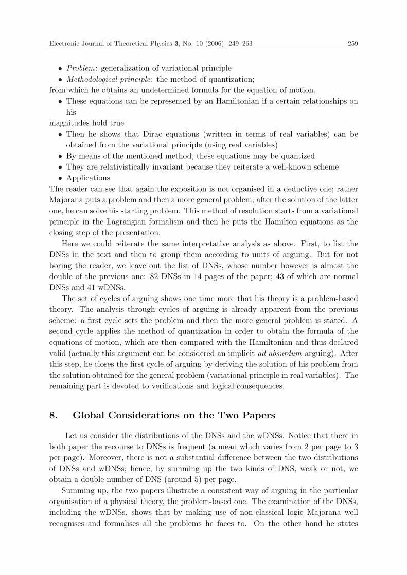
Electronic Journal of Theoretical Physics 3, No. 10 (2006) 249–263 259
• Problem: generalization of variational principle
• Methodological principle: the method of quantization;
from which he obtains an undetermined formula for the equation of motion.
• These equations can be represented by an Hamiltonian if a certain relationships on
his
magnitudes hold true
• Then he shows that Dirac equations (written in terms of real variables) can be
obtained from the variational principle (using real variables)
• By means of the mentioned method, these equations may be quantized
• They are relativistically invariant because they reiterate a well-known scheme
• Applications
The reader can see that again the exposition is not organised in a deductive one; rather
Majorana puts a problem and then a more general problem; after the solution of the latter
one, he can solve his starting problem. This method of resolution starts from a variational
principle in the Lagrangian formalism and then he puts the Hamilton equations as the
closing step of the presentation.
Here we could reiterate the same interpretative analysis as above. First, to list the
DNSs in the text and then to group them according to units of arguing. But for not
boring the reader, we leave out the list of DNSs, whose number however is almost the
double of the previous one: 82 DNSs in 14 pages of the paper; 43 of which are normal
DNSs and 41 wDNSs.
The set of cycles of arguing shows one time more that his theory is a problem-based
theory. The analysis through cycles of arguing is already apparent from the previous
scheme: a first cycle sets the problem and then the more general problem is stated. A
second cycle applies the method of quantization in order to obtain the formula of the
equations of motion, which are then compared with the Hamiltonian and thus declared
valid (actually this argument can be considered an implicit ad absurdum arguing). After
this step, he closes the first cycle of arguing by deriving the solution of his problem from
the solution obtained for the general problem (variational principle in real variables). The
remaining part is devoted to verifications and logical consequences.
8. Global Considerations on the Two Papers
Let us consider the distributions of the DNSs and the wDNSs. Notice that there in
both paper the recourse to DNSs is frequent (a mean which varies from 2 per page to 3
per page). Moreover, there is not a substantial difference between the two distributions
of DNSs and wDNSs; hence, by summing up the two kinds of DNS, weak or not, we
obtain a double number of DNS (around 5) per page.
Summing up, the two papers illustrate a consistent way of arguing in the particular
organisation of a physical theory, the problem-based one. The examination of the DNSs,
including the wDNSs, shows that by making use of non-classical logic Majorana well
recognises and formalises all the problems he faces to. On the other hand he states
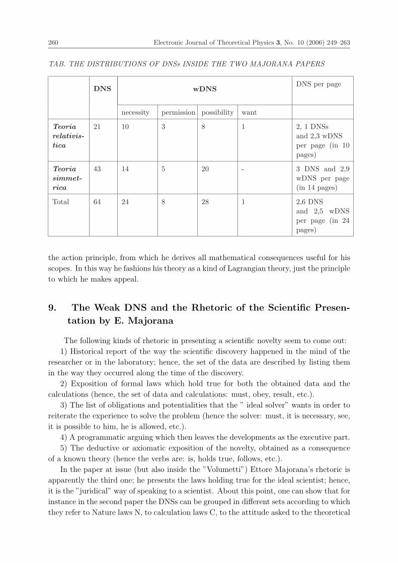
260 Electronic Journal of Theoretical Physics 3, No. 10 (2006) 249–263
TAB. THE DISTRIBUTIONS OF DNSs INSIDE THE TWO MAJORANA PAPERS
DNS wDNSDNS per page
necessity permission possibility want
Teoria
relativis-
tica
21 10 3 8 1 2, 1 DNSsand 2,3 wDNSper page (in 10pages)
Teoria
simmet-
rica
43 14 5 20 - 3 DNS and 2,9wDNS per page(in 14 pages)
Total 64 24 8 28 1 2,6 DNSand 2,5 wDNSper page (in 24pages)
the action principle, from which he derives all mathematical consequences useful for his
scopes. In this way he fashions his theory as a kind of Lagrangian theory, just the principle
to which he makes appeal.
9. The Weak DNS and the Rhetoric of the Scientific Presen-
tation by E. Majorana
The following kinds of rhetoric in presenting a scientific novelty seem to come out:
1) Historical report of the way the scientific discovery happened in the mind of the
researcher or in the laboratory; hence, the set of the data are described by listing them
in the way they occurred along the time of the discovery.
2) Exposition of formal laws which hold true for both the obtained data and the
calculations (hence, the set of data and calculations: must, obey, result, etc.).
3) The list of obligations and potentialities that the ” ideal solver” wants in order to
reiterate the experience to solve the problem (hence the solver: must, it is necessary, see,
it is possible to him, he is allowed, etc.).
4) A programmatic arguing which then leaves the developments as the executive part.
5) The deductive or axiomatic exposition of the novelty, obtained as a consequence
of a known theory (hence the verbs are: is, holds true, follows, etc.).
In the paper at issue (but also inside the ”Volumetti”) Ettore Majorana’s rhetoric is
apparently the third one; he presents the laws holding true for the ideal scientist; hence,
it is the ”juridical” way of speaking to a scientist. About this point, one can show that for
instance in the second paper the DNSs can be grouped in different sets according to which
they refer to Nature laws N, to calculation laws C, to the attitude asked to the theoretical

Electronic Journal of Theoretical Physics 3, No. 10 (2006) 249–263 261
physicist F: the maximum number is for those of kind F: 10, plus 34 wDNSs. We mean
that Majorana imposes these laws to each scientist; in this sense his presentation is more
than a ”juridical” one; it can be considered a ”royal” one.
262 Electronic Journal of Theoretical Physics 3, No. 10 (2006) 249–263
References
[1] E. Recami: Il caso Majorana, Di Renzo, Roma, 2004.
[2] The reproduction of the original manuscripts is in E. Majorana: Lezioni all’Universitadi Napoli , Bibliopolis, Napoli, 1987; for the critical edition see E. Majorana: Lezionidi Fisica Teorica, edited by S. Esposito, Bibliopolis, Napoli, 2006.
[3] S. Esposito, E. Majorana jr, E. Recami, A. van der Merwe (eds.): Ettore Majorana:Notes on Theoretical Physics, Dordrecht, Kluwer, 2003. For the original Italianedition see S. Esposito and E. Recami (eds.): Ettore Majorana: Appunti ineditidi Fisica Teorica, Zanichelli, Bologna. 2006.
[4] Reported in the letter from G. Cocconi to E. Amaldi (18 July, 1965). The letter isquoted in E. Recami: op. cit. p. 23.
[5] They are reported, for example, in the books in reference 3.
[6] E. Amaldi: La Vita e l’Opera di E. Majorana, Accad. Naz. dei Lincei, Roma, 1966.
[7] S. Esposito: Majorana solution of the Thomas-Fermi equation, Am. J. Phys. 70(2002) 852; Majorana transformation for differential equations, Int. J. Theor. Phys.41 (2002) 2417; Covariant Majorana formulation of electrodynamics, Found. Phys.28 (1998) 231; The ”Volumetti” by Ettore Majorana, in L. Gariboldi and P. Tucci(eds.): History of Physics and Astronomy in Italy in the 19 th and 20 th Centuries.Sources, themes and international context, Milano, 2004, 37-46.
[8] L. Bonolis: Giovanni Gentile ed Ettore Majorana: La comparsa della teoria dei gruppinella fisica teorica italiana, in M. Leone et al. (eds.): Atti XXII Congr. Naz. StoriaFis. e Astr., Microart, Recco GE, 2004, 117-135.
[9] A. Drago e S. Esposito: Following Weyl on Quantum Mechanics: The Contributionof Ettore Majorana, Found. Phys., 34, 2004, 871-887.
[10] E. Majorana: Teoria relativistica di particelle con momento intrinseco arbitrario,Nuovo Cimento, 9 (1932) 335-344; Teoria simmetrica dell’elettrone e del positrone,Nuovo Cimento, 14, 1937, 171.184.
[11] A. Drago: Le due opzioni, La Meridiana, Molfetta BA, 1991; in particular, pp.164-167. This kind of organisation has been recognised in several past physical,mathematical and chemical theories; its ideal model has been illustrated in A. Dragoe A. Perno: La teoria geometrica delle parallele impostata coerentemente su unproblema (I), Periodico di Mat ., ser. VIII, vol. 4, ott.-dic. 2004, 41-52 and in A.Drago: There exist two models of organization of a scientific theory, Mind and Society(in press).
[12] A. Drago: Incommensurable scientific theories: The rejection of the double negationlogical law, in D. Costantini e M. G. Galavotti (eds.): Nuovi problemi della logica edella filosofia della scienza, CLUEB, Bologna, 1991, vol. I, 195-202.
[13] A. Drago e R. Pisano: Interpretazione e ricostruzione delle Reflexions di Sadi Carnotmediante la logica non classica, Giornale di Fisica, 41 (2000) 195-215. Interpretationand reconstruction of S. Carnot’s Reflexions according to non-classical logic, AttiFond. Ronchi, 58 (2003) 195-215.
[14] L. D. Scott: ”Can a projection method of obtaining equations of motion competewith Lagrange’s equations?”, Am. J. Phys., 56 (1988) 451-456, p. 451.
[15] This conclusion was achieved by Poinsot, after forty years of unsuccesfull attemptsby the major scientists of that times, of proving the principle of virtual works:

Electronic Journal of Theoretical Physics 3, No. 10 (2006) 249–263 263
P. Bailhache, L. Poinsot: La theorie generale de l’equilibre et du mouvement dessystemes, Vrin, Paris, 1975. See also A. Drago: La Meccanica nella formulazione diLagrange: un esame storico-critico, in P. Tucci, A. Garuccio e M. Nigro (edd.): AttiXXIII Congresso Societa Italiana Storia Fisica e Astronomia, Progredit, Bari, 2003,165-179.
[16] D. Prawitz: Natural Deduction: A Proof-Theoretical Study, Almqvist & Wiksell,Stockholm, 1965.
EJTP 3, No. 10 (2006) 265–283 Electronic Journal of Theoretical Physics
Four Variations on Theoretical Physicsby Ettore Majorana
S. Esposito ∗
Dipartimento di Scienze Fisiche, Universita di Napoli “Federico II” &I.N.F.N. Sezione di Napoli,
Complesso Universitario di M. S. Angelo, Via Cinthia, 80126 Naples, Italy
Received 22 February 2006, Published 28 May 2006
Abstract: An account is given of some topical unpublished work by Ettore Majorana, revealinghis very deep intuitions and skillfulness in Theoretical Physics. The relevance of the quiteunknown results obtained by him is pointed out as wellc© Electronic Journal of Theoretical Physics. All rights reserved.
Keywords: Ettore Majorana,Thomas-Fermi equation,Electrodynamics,Lorentz GroupPACS (2006): 25.30.Pt, 13.35.Hb, 31.15.Bs, 0.3.50.De, 12.20. m
1. Introduction
Probably, the highest appraisal received by the work of Ettore Majorana was ex-
pressed by the Nobel Prize Enrico Fermi in several occasions [1], but such opinions could
appear as overstatements or unjustified (especially because they are expressed by a great
physicist as Fermi), when compared with the spare (known) Majorana’s scientific pro-
duction, just 9 published papers. However, today the name of Majorana is largely known
to the nuclear and subnuclear physicist’s community: Majorana neutrino, Majorana-
Heisenberg exchange forces, and so on are, in fact, widely used concepts.
In this paper, we focus on the less-known (or completely unknown) work by this
scientist, aimed to shed some light on the peculiar abilities of Majorana that were well
recognized by Fermi and his coworkers. The wide unpublished scientific production by
Majorana is testified by a large amount of papers [2], almost all deposited at the Domus
Galilaeana in Pisa; those known, in Italian, as “Volumetti” has been recently collected
and translated in a book [3], and we refer the interested reader to this book for further
266 Electronic Journal of Theoretical Physics 3, No. 10 (2006) 265–283
study.
Here we have chosen to discuss only four topics dealt with by Majorana in different
areas of Physics, just to give a sample of his very deep intuitions and skilfulness, together
with the relevance of the results obtained.
We start with a discussion of a peculiar approach to Quantum Mechanics, as deduced
by a manuscript [4] which probably corresponds to the text for a seminar delivered at the
University of Naples in 1938, where Majorana lectured on Theoretical Physics [5]. Some
passages of that manuscript reveal a physical interpretation of the Quantum Mechan-
ics, which anticipates of several years the Feynman approach in terms of path integrals,
independently of the underlying mathematical formulation. The main topic of that dis-
sertation was the application of Quantum Mechanics to the theory of molecular bonding,
but the present scientific interest in it is more centered on the interpretation given by
Majorana about some topics of the novel, for that time, Quantum Theory (namely, the
concept of quantum state) and the direct application of this theory to a particular case
(that is, precisely, the molecular bonding). It not only discloses a peculiar cleverness of
the author in treating a pivotal argument of the novel Mechanics, but, keeping in mind
that it was written in 1938, also reveals a net advance of at least ten years in the use
made of that topic.
In the second topic, we report on a more applicative subject, discussing an original
method that leads to a semi-analytical series solution of the Thomas -Fermi equation, with
appropriate boundary conditions, in terms of only one quadrature [6]. This was developed
by Majorana in 1928, just when starting to collaborate (still as a University student)
with the Fermi group in Rome, and reveals an outstanding ability to solve very involved
mathematical problems in a very interesting and clear way. The whole work performed on
the Thomas-Fermi model is contained in some spare sheets, and diligently reported by the
author himself in his notebooks [3]. From these it is evident the considerable contribution
given by Majorana even in the achievement of the statistical model [7], anticipating, in
many respects, some important results reached later by leading specialists. But the major
finding by Majorana was his solution (or, rather, methods of solutions) of the Thomas-
Fermi equation, which remained completely unknown, until recent times, to the Physics
community, who ignored that the non-linear differential equation relevant for atoms and
other systems could even be solved semi-analytically. The method proposed by Majorana
can also be extended to an entire class of particular differential equations [8].
Afterwards we discuss a subject that was repeatedly studied by Majorana in his
research notebooks; namely that of a formulation of Electrodynamics in terms of the
electric and magnetic fields, rather than the potentials, which is suitable for a quantum
generalization, in a complete analogy with the Dirac theory [9] [10]. This argument was
already faced in 1931 by Oppenheimer [11], who only supposed the analogy of the photon
case with that described by Dirac, but Majorana explicitly deduced a Dirac-like equation
for the photon, thus building up the presumed analogy.
Finally, we report on another topic particularly loved by Majorana, after the appear-
ance (at the end of 1928) of the seminal book by Hermann Weyl [12], that is the Group
Electronic Journal of Theoretical Physics 3, No. 10 (2006) 265–283 267
Theory and its application to physical problem. As testified by the large number of
unpublished manuscript pages of the Italian physicist, the Weyl approach greatly influ-
enced the scientific thought and work of Majorana [13]. In fact, when Majorana became
aware of the great relevance of the Weyls application of the Group Theory to Quantum
Mechanics, he immediately grabbed the Weyl method and developed it in many appli-
cations. In one of his notebooks [3] we find, for example, a preliminary study of what
will be one of the most important (published) papers by Majorana on a generalization
of the Dirac equation to particles with arbitrary spin [14]. In particular, in 1932 Majo-
rana obtained the infinite-dimensional unitary representations of the Lorentz group that
will be re-discovered by Wigner in his 1939 and 1948 works [15], and the entire theory
was re-invented by Soviet mathematicians (in particular Gel’fand and collaborators) in a
series of articles from 1948 to 1958 [16] and finally applied by physicists years later.
What presented here is, necessarily, a very short account of what Majorana really
did in his few years of work (about ten years), but, we hope, it serves in the centennial
year at least to understand the very relevant role played by him in the advancement of
Physics.
2. Path-Integral Approach to Quantum Mechanics
The usual quantum-mechanical description of a given system is strongly centered
on the role played by the hamiltonian H of the system and, as a consequence, the time
variable plays itself a key role in this description. Such a dissymmetry between space
and time variables is, obviously, not satisfactory in the light of the postulates of the
Theory of Relativity. This was firstly realized in 1932 by Dirac [17], who put forward
the idea of reformulating the whole Quantum Mechanics in terms of lagrangians rather
than hamiltonians. The starting point in the Dirac thought is that of exploiting an
analogy, holding at the quantum level, with the Hamilton principal function S in Classical
Mechanics, thus writing the transition amplitude from one space-time point to another
as an (imaginary) exponential of S. However, the original Dirac formulation was not
free from some unjustified assumptions, leading also to wrong results, and the correct
mathematical formulation and the physical interpretation of it came only in the forties
with the work by Feynman [18]. In practice, in the Feynman approach to Quantum
Mechanics, the transition amplitude between an initial and a final state can be expressed
as a sum of the factor eiS[q]/� over all the paths q with fixed end-points, not just those
corresponding to classical dynamical trajectories, for which the action is stationary.
In 1938 Majorana was appointed as full professor of Theoretical Physics at the Uni-
versity of Naples, where probably delivered a general conference mentioning also his
particular viewpoint on some basic concepts on Quantum Mechanics (see Ref. [4]). For-
tunately enough, we have some papers written by him on this subject, and few crucial
points, anticipating the Feynman approach to Quantum Mechanics, will be discussed in
the following. However, we firstly note that such papers contain nothing of the mathe-
matical aspect of that peculiar approach to Quantum Mechanics, but it is quite evident
268 Electronic Journal of Theoretical Physics 3, No. 10 (2006) 265–283
as well the presence of the physical foundations of it. This is particularly impressive if we
take into account that, in the known historical path, the interpretation of the formalism
has only followed the mathematical development of the formalism itself.
The starting point in Majorana is to search for a meaningful and clear formulation
of the concept of quantum state. And, obviously, in 1938 the dispute is opened with the
conceptions of the Old Quantum Theory.
“According to the Heisenberg theory, a quantum state corresponds not to a strangely
privileged solution of the classical equations but rather to a set of solutions which differ
for the initial conditions and even for the energy, i.e. what it is meant as precisely
defined energy for the quantum state corresponds to a sort of average over the infinite
classical orbits belonging to that state. Thus the quantum states come to be the
minimal statistical sets of classical motions, slightly different from each other, accessible
to the observations. These minimal statistical sets cannot be further partitioned due to
the uncertainty principle, introduced by Heisenberg himself, which forbids the precise
simultaneous measurement of the position and the velocity of a particle, that is the
determination of its orbit.”
Let us note that the “solutions which differ for the initial conditions” correspond, in
the Feynman language of 1948, precisely to the different integration paths. In fact, the
different initial conditions are, in any case, always referred to the same initial time (ta),
while the determined quantum state corresponds to a fixed end time (tb). The introduced
issue of “slightly different classical motions” (the emphasis is given by Majorana himself),
according to what specified by the Heisenberg’s uncertainty principle and mentioned just
afterwards, is thus evidently related to that of the sufficiently wide integration region
required in the Feynman path-integral formula for quantum (rather than classical) sys-
tems. In this respect, such a mathematical point is intimately related to a fundamental
physical principle.
The crucial point in the Feynman formulation of Quantum Mechanics is, as well-
known, to consider not only the paths corresponding to classical trajectories, but all the
possible paths joining the initial point with the end one. In the Majorana manuscript,
after a discussion on an interesting example on the harmonic oscillator, the author points
out:
“Obviously the correspondence between quantum states and sets of classical solutions is
only approximate, since the equations describing the quantum dynamics are in general
independent of the corresponding classical equations, but denote a real modification of
the mechanical laws, as well as a constraint on the feasibility of a given observation;
however it is better founded than the representation of the quantum states in terms of
quantized orbits, and can be usefully employed in qualitative studies.”
And, in a later passage, it is more explicitly stated that the wave function “corresponds
in Quantum Mechanics to any possible state of the electron”. Such a reference, that only
superficially could be interpreted, in the common acceptation, that all the information
on the physical systems is contained in the wave function, should instead be considered
in the meaning given by Feynman, according to the comprehensive discussion made by
Electronic Journal of Theoretical Physics 3, No. 10 (2006) 265–283 269
Majorana on the concept of state.
Finally we point out that, in the Majorana analysis, a key role is played by the
symmetry properties of the physical system.
“Under given assumptions, that are verified in the very simple problems which we will
consider, we can say that every quantum state possesses all the symmetry properties
of the constraints of the system.”
The relationship with the path-integral formulation is made as follows. In discussing a
given atomic system, Majorana points out how from one quantum state S of the system
we can obtain another one S ′ by means of a symmetry operation.
“However, differently from what happens in Classical Mechanics for the single solutions
of the dynamical equations, in general it is no longer true that S ′ will be distinct from
S. We can realize this easily by representing S ′ with a set of classical solutions, as
seen above; it then suffices that S includes, for any given solution, even the other one
obtained from that solution by applying a symmetry property of the motions of the
systems, in order that S ′ results to be identical to S.”
This passage is particularly intriguing if we observe that the issue of the redundant
counting in the integration measure in gauge theories, leading to infinite expressions for
the transition amplitudes, was raised (and solved) only after much time from the Feynman
paper.
3. Solution of the Thomas-Fermi Equation
The main idea of the Thomas-Fermi atomic model is that of considering the elec-
trons around the nucleus as a gas of particles, obeying the Pauli exclusion principle, at
the absolute zero of temperature. The limiting case of the Fermi statistics for strong
degeneracy applies to such a gas. Then, in this approximation, the potential V inside a
given atom of charge number Z at a distance r from the nucleus may be written as
V (r) =Ze
rϕ(r). (1)
With a suitable change of variable, r = μx and
μ =1
2
(3π
4
)2/3�2
mee2Z−1/3, (2)
the Thomas-Fermi function ϕ satisfies the following non-linear differential equation (for
ϕ > 0):
ϕ′′ =ϕ3/2
√x
(3)
(a prime denotes differentiation with respect to x) with the boundary conditions:
ϕ(0) = 1,
ϕ(∞) = 0.
(4)
270 Electronic Journal of Theoretical Physics 3, No. 10 (2006) 265–283
The Fermi equation (3) is a universal equation which does not depend neither on Z nor on
physical constants (�,m, e). Its solution gives, from Eq. (1), as noted by Fermi himself, a
screened Coulomb potential which at any point is equal to that produced by an effective
charge
Ze ϕ
(r
μ
). (5)
As was immediately realized, in force of the independence of Eq. (3) on Z, the method
gives an effective potential which can be easily adapted to describe any atom with a
suitable scaling factor, according to Eq. (5).
The problem of the theoretical calculation of observable atomic properties is thus
solved, in the Thomas-Fermi approximation, in terms of the function ϕ(x) introduced
in Eq. (1) and satisfying the Fermi differential equation (3). By using standard but
involved mathematical tools, in his paper [19] Thomas got an exact, “singular” solution
of his differential equation satisfying only the second condition (4). This was later (in
1930) considered by Sommerfeld [20] as an approximation of the function ϕ(x) for large
x (and is indeed known as the “Sommerfeld solution” of the Fermi equation),
ϕ(x) =144
x3, (6)
and Sommerfeld himself obtained corrections to the above quantity in order to approxi-
mate in a better way the function ϕ(x) for not extremely large values of x.
Until recent times it has been believed that the solution of such equation satisfying
both the appropriate boundary conditions in (4) cannot be expressed in closed form, and
some effort has been made, starting from Thomas [19], Fermi [21], [22] and others, in order
to achieve the numerical integration of the differential equation. However, we now know
[6], [7] that Majorana in 1927-8 found a semi-analytical solution of the Thomas-Fermi
equation by applying a novel exact method [8]. Before proceeding, we will indulge here
on an anecdote reported by Rasetti [23], Segre [24] and Amaldi [25]. According to the last
author, “Fermi gave a broad outline of the model and showed some reprints of his recent
works on the subject to Majorana, in particular the table showing the numerical values
of the so-called Fermi universal potential. Majorana listened with interest and, after
having asked for some explanations, left without giving any indication of his thoughts or
intentions. The next day, towards the end of the morning, he again came into Fermi’s
office and asked him without more ado to draw him the table which he had seen for
few moments the day before. Holding this table in his hand, he took from his pocket a
piece of paper on which he had worked out a similar table at home in the last twenty-
four hours, transforming, as far as Segre remembers, the second-order Thomas-Fermi
non-linear differential equation into a Riccati equation, which he had then integrated
numerically.”
The whole work performed by Majorana on the solution of the Fermi equation, is
contained in some spare sheets conserved at the Domus Galilaeana in Pisa, and diligently
reported by the author himself in his notebooks [3]. The reduction of the Fermi equation
to an Abel equation (rather than a Riccati one, as confused by Segre) proceeds as follows.
Electronic Journal of Theoretical Physics 3, No. 10 (2006) 265–283 271
Let’s adopt a change of variables, from (x, ϕ) to (t, u), where the formula relating the two
sets of variables has to be determined in order to satisfy, if possible, both the boundary
conditions (4). The function ϕ in Eq. (6) has the correct behavior for large x, but the
wrong one near x = 0, so that we could modify the functional form of ϕ to take into
account the first condition in (4). An obvious modification is ϕ = (144/x3)f(x), with f(x)
a suitable function which vanishes for x → 0 in order to account for ϕ(x = 0) = 1. The
simplest choice for f(x) is a polynomial in the novel variable t, as it was also considered
later, in a similar way, by Sommerfeld [20]. The Majorana choice is as follows:
ϕ(x) =144
x3(1− t)2, (7)
with t → 1 as x → 0. From Eq. (7) we can then obtain the first relation linking t to
x, ϕ. The second one, involving the dependent variable u, is that typical of homogeneous
differential equations (like the Fermi equation) for reducing the order of the equation, i.e.
exponentiation with an integral of u(t). The transformation relations are thus:
t = 1− 1
12
√x3ϕ,
ϕ = e� t1 u(t)dt .
(8)
Substitution into Eq. (3) leads to an Abel equation for u(t),
du
dt= α(t) + β(t) u + γ(t) u2 + δ(t) u3, (9)
with
α(t) =16
3(1− t),
β(t) = 8 +1
3(1− t),
γ(t) =7
3− 4t,
δ(t) = −2
3t(1− t).
(10)
Note that both the boundary conditions in (4) are automatically verified by the relations
(8). We have reported the derivation of the Abel equation (9) mainly for historical
reasons (nevertheless, it is quite important since, in this way, all the theorems on the
Abel equation may thus be applied to the non-linear Thomas-Fermi equation too); the
precise numerical values for the Fermi function ϕ(x) were obtained by Majorana by
272 Electronic Journal of Theoretical Physics 3, No. 10 (2006) 265–283
solving a different first-order differential equation. Instead of Eq. (7), Majorana chooses
ϕ(x) of the form
ϕ(x) =144
x3t6. (11)
Now the point with x = 0 corresponds to t = 0. In order to obtain again a first order
differential equation for u(t), the transformation equation for the variable u involves ϕ
and its first derivative. Majorana then introduced the following formulas:
t = 144−1/6 x1/2 ϕ1/6,
u = −(
16
3
)1/3
ϕ−4/3ϕ′ .
(12)
By taking the t-derivative of the last equation in (12) and inserting Eq. (3) in it, one
gets:
du
dt= −
(16
3
)1/3
xϕ−4/3
[−4
3
ϕ′2
ϕ+
ϕ3/2
x1/2
]. (13)
By using Eqs. (12) to eliminate x1/2 and ϕ′2, the following equation results:
du
dt=
(4
9
)1/3tu2 − 1
txϕ1/3. (14)
Now the quantity xϕ1/3 can be expressed in terms of t and u by making use again of the
first equation in (12) (and its t-derivative). After some algebra, the final result for the
differential equation for u(t) is:du
dt= 8
tu2 − 1
1− t2u. (15)
The obtained equation is again non-linear but, differently from the original Fermi equation
(3), it is first-order in the novel variable t and the degree of non-linearity is lower than
that of Eq. (3). The boundary conditions for u(t) are easily taken into account from the
second equation in (12) and by requiring that for x → ∞ the Sommerfeld solution (Eq.
(11) with t = 1) be recovered:
u(0) = −(
16
3
)1/3
ϕ′0,
u(1) = 1.
(16)
Here we have denoted with ϕ′0 = ϕ′(x = 0) the initial slope of the Thomas-Fermi function
ϕ(x) which, for a neutral atom, is approximately equal to −1.588.
The solution of Eq. (15) was achieved by Majorana in terms of a series expansion in
powers of the variable τ = 1− t:
u = a0 + a1τ + a2τ2 + a3τ
3 + ... . (17)
Electronic Journal of Theoretical Physics 3, No. 10 (2006) 265–283 273
Substitution of Eq. (17) (with the conditions in Eq. (16)) into Eq. (15) results into an
iterative formula for the coefficients an (for details see Ref. [6]). It is remarkable that
the series expansion in Eq. (17) is uniformly convergent in the interval [0, 1] for τ , since
the series∑∞
n=0 an of the coefficients converges to a finite value determined by the initial
slope ϕ′0. In fact, by setting τ = 1 (t = 0) in Eq. (17) we have from Eq. (16):
∞∑n=0
an = −(
16
3
)ϕ′
0 (18)
Majorana was aware [3] of the fact that the series in Eq. (17) exhibits geometrical
convergence with an/an−1 ∼ 4/5 for n → ∞. Given the function u(t), we now have
to look for the Thomas-Fermi function ϕ(x). This was obtained in a parametric form
x = x(t), ϕ = ϕ(t) in terms of the parameter t already introduced in Eq. (12), and by
writing ϕ(t) as
ϕ(t) = e� t0 w(t)dt (19)
(with this choice, ϕ(t = 0) = 1 and the first condition in (4) is automatically satisfied).
Here w(t) is an auxiliary function which is determined in terms of u(t) by substituting
Eq. (19) into Eq. (12). As a result, the parametric solution of Eq. (3), with boundary
conditions (4), takes the form:
x(t) = 1441/3 t2 e2I(t)
ϕ(t) = e−6 I(t)
(20)
with
I(t) =
∫ t
0
ut
1− t2udt (21)
Remarkably, the Majorana solution of the Thomas-Fermi equation is obtained with only
one quadrature and gives easily obtainable numerical values for the electrostatic potential
inside atoms. By taking into account only 10 terms in the series expansion for u(t),
such numerical values approximate the values of the exact solution of the Thomas-Fermi
equation with a relative error of the order of 0.1%.
The intriguing property in the Majorana derivation of the solution of the Thomas-
Fermi equation is that his method can be easily generalized and may be applied to a large
class of particular differential equations, as discussed in [8].
Several generalizations of the Thomas-Fermi method for atoms were proposed as early
as in 1928 by Majorana, but they were considered by the physics community, ignoring
the Majorana unpublished works, only many years later.
Indeed, in Sect. 16 of Volumetto II [3], Majorana studied the problem of an atom in
a weak external electric field E, i.e. atomic polarizability, and obtained an expression for
the electric dipole moment for a (neutral or arbitrarily ionized) atom.
Furthermore, he also started to consider the application of the statistical method
to molecules, rather than single atoms, studying the case of a diatomic molecule with
274 Electronic Journal of Theoretical Physics 3, No. 10 (2006) 265–283
identical nuclei (see Sect. 12 of Volumetto II [3]). The effective potential in the molecule
was cast in the form:
V = V1 + V2 − α2V1V2
V1 + V2
, (22)
V1 and V2 being the potentials generated by each of the two atoms. The function α must
obey the differential equation for V ,
∇2V = −kV 3/2 (23)
(k is a suitable constant), with appropriate boundary conditions, discussed in [3]. Ma-
jorana also gave a general method to determine V when the equipotential surfaces are
approximately known (see Sect. 12 of Volumetto III [3]). In fact, writing the approximate
expression for the equipotential surfaces, as functions of a parameter p, as
f(x, y, z) = p, (24)
he deduced a thorough equation from which it is possible to determine V (ρ), when the
boundary conditions are assigned. The particular case of a diatomic molecule with iden-
tical nuclei was, again, considered by Majorana using elliptic coordinates in order to
illustrate his original method [3].
Finally, our author also considered the second approximation for the potential inside
the atom, beyond the Thomas-Fermi one, with a generalization of the statistical model
of neutral atoms to those ionized n times, including the case n = 0 (see Sect. 15 of
Volumetto II [3]). As recently pointed out, the approach used by Majorana to this end
is rather similar to that now adopted in the renormalization of physical quantities in
modern gauge theories [26].
4. Majorana Formulation of Electrodynamics
In 1931, in his “note on light quanta and the electromagnetic field” [11], Oppenheimer
developed an alternative model to the theory of Quantum Electrodynamics, starting from
an analogy with the Dirac theory of the electron. Such a formulation was particularly
held dear by Majorana, who studied it in some of his unpublished notebooks [9].
Majorana’s original idea was that if the Maxwell theory of electromagnetism has to
be viewed as the wave mechanics of the photon, then it must be possible to write the
Maxwell equations as a Dirac-like equation for a probability quantum wave ψ, this wave
function being expressible by means of the physical �E , �B fields. This can be, indeed,
realized introducing the quantity
�ψ = �E − i �B (25)
since �ψ∗·�ψ = �E2 + �B2 is directly proportional to the probability density function for a
photon 1. In terms of �ψ, the Maxwell equations in vacuum then write
�∇·�ψ = 0 (26)
1 If we have a beam of n equal photons each of them with energy ε (given by the Planck relation),
Electronic Journal of Theoretical Physics 3, No. 10 (2006) 265–283 275
∂ �ψ
∂t= i �∇×�ψ (27)
By making use of the correspondence principle
E → i∂
∂t(28)
�p→ −i �∇ (29)
these equations effectively can be cast in a Dirac-like form
(E − α·�p) �ψ = 0 (30)
with the transversality condition
�p·�ψ = 0 (31)
where the 3x3 hermitian matrices (αi)lm = i εilm
α1 =
⎛⎜⎜⎜⎜⎝0 0 0
0 0 i
0 −i 0
⎞⎟⎟⎟⎟⎠ α2 =
⎛⎜⎜⎜⎜⎝0 0 −i
0 0 0
i 0 0
⎞⎟⎟⎟⎟⎠ α3 =
⎛⎜⎜⎜⎜⎝0 i 0
−i 0 0
0 0 0
⎞⎟⎟⎟⎟⎠ (32)
satisfying
[αi , αj] = −i εijk αk (33)
have been introduced.
The probabilistic interpretation is indeed possible given the “continuity equation”
(Poynting theorem)∂ρ
∂t+ �∇·�j = 0 (34)
where
ρ =1
2�ψ∗·�ψ �j = − 1
2ψ∗ α ψ (35)
are respectively the energy and momentum density of the electromagnetic field.
It is interesting to observe that, differently from Oppenheimer, who started from
a mere, presumed analogy with the electron case, Majorana built on analytically the
analogy with the Dirac theory, at a dynamical level, by deducing the Dirac-like equation
for the photon from the Maxwell equations with the introduction of a complex wave field.
As noted by Giannetto in Ref. [10], the Majorana formulation is algebraically equivalent
to the standard one of Quantum Electrodynamics and, in addition, also some relevant
problems concerning the negative energy states, that induced Oppenheimer to abandon
his model, may be elegantly solved by using the method envisaged in a later work [27],
thus giving further physical insight into Majorana theory.
since 12 (�E2 + �B2) is the energy density of the electromagnetic field, then 1
nε12 (�E2 + �B2) dS dt gives the
probability that each photon has to be detected in the area dS in the time dt. The generalization tophotons of different energies (i.e. of different frequencies) is obtained with the aid of the superpositionprinciple.
276 Electronic Journal of Theoretical Physics 3, No. 10 (2006) 265–283
5. Lorentz Group and its Applications
The important role of symmetries in Quantum Mechanics was established in the
third decade of the XX century, when it was discovered the special relationships con-
cerning systems of identical particles, reflection and rotational symmetry or translation
invariance. Very soon it was discovered that the systematic theory of symmetry resulted
to be just a part of the mathematical theory of groups, as pointed out, for example, in the
reference book by H. Weyl [12]. A particularly intriguing example is that of the Lorentz
group which, as well known, underlies the Theory of Relativity, and its representations
are especially relevant for the Dirac equation in Relativistic Quantum Mechanics. In the
mentioned book, however, although the correspondence between the Dirac equation and
the Lorentz transformations is pointed out, the group properties of this connection are
not highlighted. Moreover, only a particular kind of such representations are considered
(those related to the two-dimensional representations of the group of rotations, according
to Pauli), but an exhaustive study of this subject was still lacking at that time.
The situation changes [13] quite sensibly with several (unpublished) papers by Ma-
jorana [3], where he gives a detailed deduction of the relationship between the repre-
sentations of the Lorentz group and the matrices of the (special) unitary group in two
dimensions, and a strict connection with the Dirac equation is always taken into account.
Moreover the explicit form of the transformations of every bilinear in the spinor field Ψ
is reported. For example, Majorana obtains that some of such bilinears behave as the
4-position vector (ct, x, y, z) or as the components of the rank-2 electromagnetic tensor
( �E, �H) under Lorentz transformations, according to the following rules:
Ψ†Ψ ∼ −iΨ†αxαyαzΨ ∼ ct,
−Ψ†αxΨ ∼ iΨ†αyαzΨ ∼ x,
−Ψ†αyΨ ∼ iΨ†αzαxΨ ∼ y,
−Ψ†αzΨ ∼ iΨ†αxαyΨ ∼ z,
iΨ†βαxΨ ∼ Ex, iΨ†βαyΨ ∼ Ey, iΨ†βαzΨ ∼ Ez,
iΨ†βαyαzΨ ∼ Hx, iΨ†βαzαxΨ ∼ Hy, iΨ†βαxαyΨ ∼ Hz,
Ψ†βΨ ∼ Ψ†βαxαyαzΨ ∼ 1,
where αx, αy, αz, β are Dirac matrices. But, probably, the most important result achieved
by Majorana on this subject is his discussion of infinite-dimensional unitary represen-
tations of the Lorentz group, giving also an explicit form for them. Note that such
representations were independently discovered by Wigner in 1939 and 1948 [15] and were
thoroughly studied only in the years 1948-1958 [16]. Lucky enough, we are able to
reconstruct the reasoning which led Majorana to discuss the infinite-dimensional repre-
sentations. In Sect. 8 of Volumetto V we read [3]:
“The representations of the Lorentz group are, except for the identity representation,
essentially not unitary, i.e., they cannot be converted into unitary representations by
some transformation. The reason for this is that the Lorentz group is an open group.
However, in contrast to what happens for closed groups, open groups may have irre-
Electronic Journal of Theoretical Physics 3, No. 10 (2006) 265–283 277
ducible representations (even unitary) in infinite dimensions. In what follows, we shall
give two classes of such representations for the Lorentz group, each of them composed
of a continuous infinity of unitary representations.”
The two classes of representations correspond to integer and half-integer values for the
representation index j (angular momentum). Majorana begins by noting that the group
of the real Lorentz transformations acting on the variables ct, x, y, z can be constructed
from the infinitesimal transformations associated to the matrices:
Sx =
⎛⎜⎜⎜⎜⎜⎜⎜⎝
0 0 0 0
0 0 0 0
0 0 0 −1
0 0 1 0
⎞⎟⎟⎟⎟⎟⎟⎟⎠, Sy =
⎛⎜⎜⎜⎜⎜⎜⎜⎝
0 0 0 0
0 0 0 1
0 0 0 0
0 −1 0 0
⎞⎟⎟⎟⎟⎟⎟⎟⎠,
Sz =
⎛⎜⎜⎜⎜⎜⎜⎜⎝
0 0 0 0
0 0 −1 0
0 1 0 0
0 0 0 0
⎞⎟⎟⎟⎟⎟⎟⎟⎠,
Tx =
⎛⎜⎜⎜⎜⎜⎜⎜⎝
0 1 0 0
1 0 0 0
0 0 0 0
0 0 0 0
⎞⎟⎟⎟⎟⎟⎟⎟⎠, Ty =
⎛⎜⎜⎜⎜⎜⎜⎜⎝
0 0 1 0
0 0 0 0
1 0 0 0
0 0 0 0
⎞⎟⎟⎟⎟⎟⎟⎟⎠,
Tz =
⎛⎜⎜⎜⎜⎜⎜⎜⎝
0 0 0 1
0 0 0 0
0 0 0 0
1 0 0 0
⎞⎟⎟⎟⎟⎟⎟⎟⎠,
(36)
from which he deduces the general commutation relations satisfied by the S and T oper-
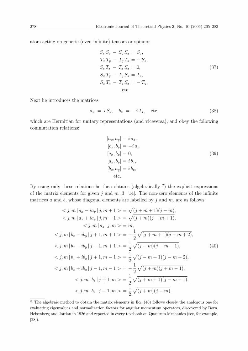
278 Electronic Journal of Theoretical Physics 3, No. 10 (2006) 265–283
ators acting on generic (even infinite) tensors or spinors:
Sx Sy − Sy Sx = Sz,
Tx Ty − Ty Tx = −Sz,
Sx Tx − Tx Sx = 0, (37)
Sx Ty − Ty Sx = Tz,
Sx Tz − Tz Sx = −Ty,
etc.
Next he introduces the matrices
ax = i Sx, bx = −i Tx, etc. (38)
which are Hermitian for unitary representations (and viceversa), and obey the following
commutation relations:
[ax, ay] = i az,
[bx, by] = −i az,
[ax, bx] = 0, (39)
[ax, by] = i bz,
[bx, ay] = i bz,
etc.
By using only these relations he then obtains (algebraically 2) the explicit expressions
of the matrix elements for given j and m [3] [14]. The non-zero elements of the infinite
matrices a and b, whose diagonal elements are labelled by j and m, are as follows:
< j, m | ax − iay | j, m + 1 > =√
(j + m + 1)(j −m),
< j, m | ax + iay | j,m− 1 > =√
(j + m)(j −m + 1),
< j,m | az | j,m > = m,
< j,m | bx − iby | j + 1,m + 1 > = − 1
2
√(j + m + 1)(j + m + 2),
< j, m | bx − iby | j − 1,m + 1 > =1
2
√(j −m)(j −m− 1), (40)
< j,m | bx + iby | j + 1,m− 1 > =1
2
√(j −m + 1)(j −m + 2),
< j, m | bx + iby | j − 1,m− 1 > = − 1
2
√(j + m)(j + m− 1),
< j, m | bz | j + 1,m > =1
2
√(j + m + 1)(j −m + 1),
< j, m | bz | j − 1,m > =1
2
√(j + m)(j −m).
2 The algebraic method to obtain the matrix elements in Eq. (40) follows closely the analogous one forevaluating eigenvalues and normalization factors for angular momentum operators, discovered by Born,Heisenberg and Jordan in 1926 and reported in every textbook on Quantum Mechanics (see, for example,[28]).
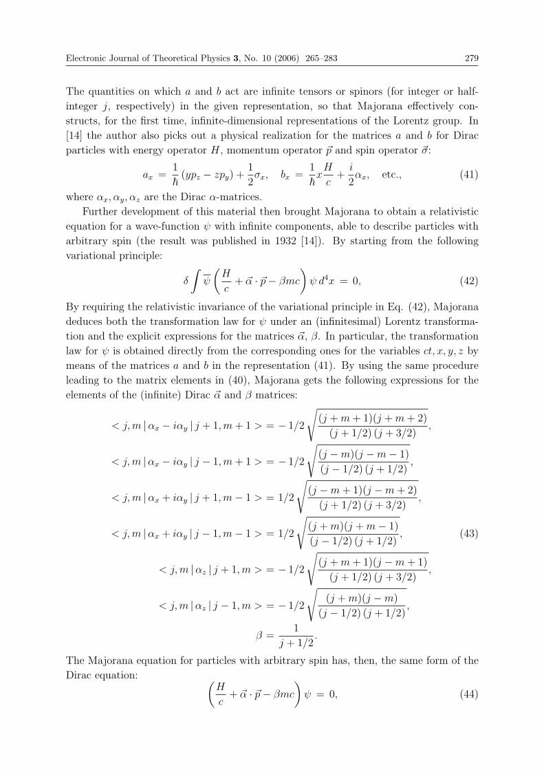
Electronic Journal of Theoretical Physics 3, No. 10 (2006) 265–283 279
The quantities on which a and b act are infinite tensors or spinors (for integer or half-
integer j, respectively) in the given representation, so that Majorana effectively con-
structs, for the first time, infinite-dimensional representations of the Lorentz group. In
[14] the author also picks out a physical realization for the matrices a and b for Dirac
particles with energy operator H, momentum operator �p and spin operator �σ:
ax =1
�(ypz − zpy) +
1
2σx, bx =
1
�xH
c+
i
2αx, etc., (41)
where αx, αy, αz are the Dirac α-matrices.
Further development of this material then brought Majorana to obtain a relativistic
equation for a wave-function ψ with infinite components, able to describe particles with
arbitrary spin (the result was published in 1932 [14]). By starting from the following
variational principle:
δ
∫ψ
(H
c+ �α · �p− βmc
)ψ d4x = 0, (42)
By requiring the relativistic invariance of the variational principle in Eq. (42), Majorana
deduces both the transformation law for ψ under an (infinitesimal) Lorentz transforma-
tion and the explicit expressions for the matrices �α, β. In particular, the transformation
law for ψ is obtained directly from the corresponding ones for the variables ct, x, y, z by
means of the matrices a and b in the representation (41). By using the same procedure
leading to the matrix elements in (40), Majorana gets the following expressions for the
elements of the (infinite) Dirac �α and β matrices:
< j, m |αx − iαy | j + 1,m + 1 > = − 1/2
√(j + m + 1)(j + m + 2)
(j + 1/2) (j + 3/2),
< j,m |αx − iαy | j − 1,m + 1 > = − 1/2
√(j −m)(j −m− 1)
(j − 1/2) (j + 1/2),
< j, m |αx + iαy | j + 1,m− 1 > = 1/2
√(j −m + 1)(j −m + 2)
(j + 1/2) (j + 3/2),
< j,m |αx + iαy | j − 1,m− 1 > = 1/2
√(j + m)(j + m− 1)
(j − 1/2) (j + 1/2), (43)
< j, m |αz | j + 1,m > = − 1/2
√(j + m + 1)(j −m + 1)
(j + 1/2) (j + 3/2),
< j,m |αz | j − 1,m > = − 1/2
√(j + m)(j −m)
(j − 1/2) (j + 1/2),
β =1
j + 1/2.
The Majorana equation for particles with arbitrary spin has, then, the same form of the
Dirac equation: (H
c+ �α · �p− βmc
)ψ = 0, (44)
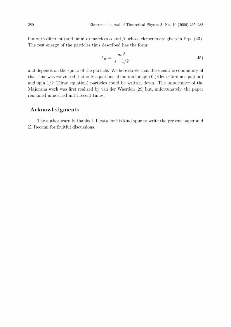
280 Electronic Journal of Theoretical Physics 3, No. 10 (2006) 265–283
but with different (and infinite) matrices α and β, whose elements are given in Eqs. (43).
The rest energy of the particles thus described has the form:
E0 =mc2
s + 1/2, (45)
and depends on the spin s of the particle. We here stress that the scientific community of
that time was convinced that only equations of motion for spin 0 (Klein-Gordon equation)
and spin 1/2 (Dirac equation) particles could be written down. The importance of the
Majorana work was first realized by van der Waerden [29] but, unfortunately, the paper
remained unnoticed until recent times.
Acknowledgments
The author warmly thanks I. Licata for his kind spur to write the present paper and
E. Recami for fruitful discussions.
Electronic Journal of Theoretical Physics 3, No. 10 (2006) 265–283 281
References
[1] See the contribution by E. Recami in this volume.
[2] The list of the unpublished scientific manuscripts by Majorana can be found in E.Recami, Quaderni di Storia della Fisica, 5 (1999) 19.
[3] S. Esposito, E. Majorana jr, A. van der Merwe and E. Recami (eds.) Ettore Majorana:Notes on Theoretical Physics (Kluwer, New York, 2003).
[4] S. Esposito, Quaderni di Storia della Fisica, preprint; arXiv:physics/0512174.
[5] E. Majorana, Lezioni all’Universita di Napoli, (Bibliopolis, Napoli, 1987). E.Majorana, Lezioni di Fisica Teorica, edited by S. Esposito (Bibliopolis, Napoli, 2006).S. Esposito, Il Nuovo Saggiatore, 21 (2005) 21; A. Drago and S. Esposito, e-printarXiv:physics/0503084.
[6] S. Esposito, Am. J. Phys. 70 (2002) 852; arXiv:physics/0111167.
[7] E. Di Grezia and S. Esposito, Found. Phys. 34 (2004) 1431; e-printarXiv:physics/0406030.
[8] S. Esposito, Int. J. Theor. Phys. 41 (2002) 2417; e-print arXiv:math-ph/0204040.
[9] R. Mignani, E. Recami and M. Baldo, Lett. Nuovo Cim. 11 (1974) 568; see also E.Giannetto, Lett. Nuovo Cim. 44 (1985) 140 and 145. S. Esposito, Found. Phys. 28(1998) 231; e-print arXiv:hep-th/9704144.
[10] E. Giannetto, in F. Bevilacqua (ed.) Atti IX Congresso Naz.le di Storia della Fisica(Milan, 1988) p.173.
[11] J.R. Oppenheimer, Phys. Rev. 38 (1931) 725.
[12] H. Weyl, Gruppentheorie und Quantenmechanik, first edition (Hirzel, Leipzig, 1928);English translation from the second German edition in The Theory of Groups andQuantum Mechanics (Dover, New York 1931).
[13] A. Drago and S. Esposito, Found. Phys. 34 (2004) 871; arXiv:physics/0503084.
[14] E. Majorana, Nuovo Cim. 9 (1932) 335.
[15] E. Wigner, Ann. Math. 40 (1939) 149.
[16] I.M. Gel’fand, A.M. Yaglom, Zh. Ehksp. Teor. Fiz. 18 (1948) 703; I.M. Gel’fand,R.A. Minlos, Z.Ya. Shapiro, Representations of the Rotation and Lorentz Groups andtheir Applications (Pergamon Press, Oxford, 1963).
[17] P. A. M. Dirac, Phys. Zeits. Sowjetunion 3 (1933) 64.
[18] R. P. Feynman, The Principle of Least Action in Quantum Mechanics (PrincetonUniversity, Ann Arbor, 1942; University Microfilms Publication No. 2948). R. P.Feynman, Rev. Mod. Phys. 20 (1948) 367.
[19] L.H. Thomas, Proc. Camb. Phil. Soc. 23 (1926) 542.
[20] A. Sommerfeld, Rend. Lincei 15 (1932) 788.
[21] E. Fermi, Rend. Lincei 6 (1927) 602.
[22] E. Fermi, Falkenhagen, Quantentheorie und Chemie, Leipziger Vortraege 95 (1928).
282 Electronic Journal of Theoretical Physics 3, No. 10 (2006) 265–283
[23] F. Rasetti in E. Fermi Collected Papers (Note e Memorie) (University of ChicagoPress, Chicago, 1962) p. 277.
[24] E. Segre, A Mind Always in Motion (University of California Press, Berkeley, 1993).
[25] E. Amaldi, Ettore Majorana: Man and Scientist, in A. Zichichi (ed.) Strong andWeak Interactions. Present problems (Academic Press, New York, 1966).
[26] S. Esposito, preprint arXiv:physics/0512259.
[27] E. Majorana, Nuovo Cim. 14 (1937) 171.
[28] J.J. Sakurai, Modern Quantum Mechanics (Benjamin-Cummings, Menlo Park, 1985).
[29] Letter from Leipzig by Ettore Majorana to his father dated February 18, 1933, quotedby Recami in Ettore Majorana, Lezioni all’Universita di Napoli in [5].
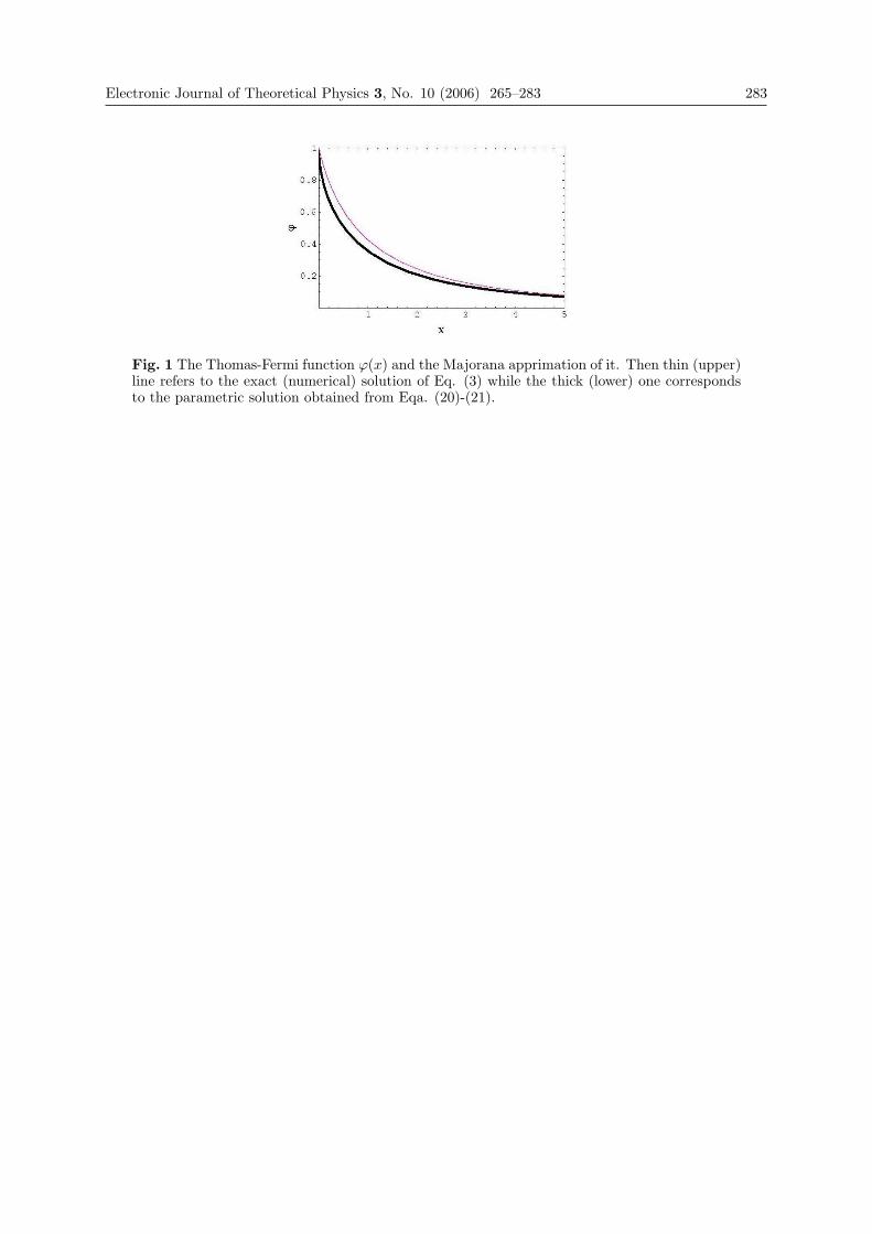
Electronic Journal of Theoretical Physics 3, No. 10 (2006) 265–283 283
Fig. 1 The Thomas-Fermi function ϕ(x) and the Majorana apprimation of it. Then thin (upper)line refers to the exact (numerical) solution of Eq. (3) while the thick (lower) one correspondsto the parametric solution obtained from Eqa. (20)-(21).
EJTP 3, No. 10 (2006) 285–292 Electronic Journal of Theoretical Physics
The Majorana Oscillator
Eliano Pessa ∗
Centro Interdipartimentale di Scienze Cognitive,Universita di Pavia.Piazza Botta 6,27100 Pavia, Italy
Received 26 April 2006, Published 28 May 2006
Abstract: At present the expression ‘Majorana oscillator’ does not appear to be in use intheoretical physics. However, the author of this paper heard it in the Seventies, during privateconversations with the late Prof. B.Touschek. This little contribution tries to explore thepossible meanings of this expression and introduces a new field equation, generalizing theone already introduced by Majorana himself, which could describe a hypothetical ‘Majoranaoscillator’.c© Electronic Journal of Theoretical Physics. All rights reserved.
Keywords: Majorana Oscillator, Majorana EquationPACS (2006): 03.65.Pm, 11.10.-z, 03.70.+k
1. Introduction
The Majorana oscillator came into my life around 1976. At that time I was student
at the postgraduate school in Physics of the University of Rome, Italy. In this regard I
need to remind younger physicists of the lack, within the university system holding in
Italy at that time, of the PhD degree. The highest attainable degree was the one given
by postgraduate schools, typically after two years of hard work and the discussion of a
final thesis. In Italy, however, there were very few schools of this kind, and limited to a
small number of disciplinary domains. Fortunately the latter included Physics and such
a circumstance had given me the opportunity of attending the courses of postgraduate
school existing in the University of Rome (named ‘Scuola di Perfezionamento in Fisica’).
The scientific level of the latter was very high, more or less comparable to the one of
present PhD schools. From 1974 to 1976 I worked at my final thesis, dealing with the
process of particle creation by a quantum field embedded in a Riemannian space, under
the supervision of the late Prof. Bruno Touschek. His name being widely known among
286 Electronic Journal of Theoretical Physics 3, No. 10 (2006) 285–292
physicists, I don’t need an illustration of his outstanding contributions to the develop-
ment of Physics (the introduction of storage rings and the theory of neutrino would be
enough), which are not the subject of this paper. I will limit myself to mention the fact
that throughout these two years (and even later) I was engaged in frequent and long
discussions with Prof. Touschek about the subject of my thesis and, chiefly, about the
very foundations of Quantum Field Theory. At the beginning of 1976 I had completed my
work and finished all computations. However, I was not satisfied with my results, which
I considered only as approximate, owing to the fact that I had realized a deep conceptual
incompleteness of Quantum Field Theory itself. The latter was the subject of a number of
discussions with Prof. Touschek, which took place up to the Avril 1976 (when I discussed
my thesis), in which, typically, I started by criticizing specific aspects of Quantum Field
Theory, so as to stimulate him to answering me, or by showing the inconsistence of my
arguments or by making new proposals for overcoming the limits of theoretical schemata
used at that time. In particular, I remember that one day (I forgot the exact date) I
started by claiming that Quantum Field Theory could not be considered as consistent
with Special Relativity, as it was heavily based on a concept of ‘oscillator’ entirely drawn
from traditional classical mechanics. To be more coherent with Special Relativity – I
maintained – one should start by relying on a theory of special-relativistic oscillators and
then shaping on it the whole formalism. It was during the ensuing discussion that Prof.
Touschek used the term ‘Majorana oscillator’. At that time I was young and – as it is
often the case – very ignorant. Of course, I knew very well the name of Majorana, but
not his theory of neutrino. So I thought that the expression ‘Majorana oscillator’ were
denoting a concept widely known among theoretical physicists, but unknown to me (a
circumstance, the latter, which it was better not to underline), and in this way I missed
the occasion for asking Prof. Touschek about this subject. Long after, when talking
with other physicists, I was surprised in realizing that nobody knew the meaning of the
expression ‘Majorana oscillator’. On the contrary, my colleagues asked me for more in-
formation about this concept. When I undertook a search, on books, journals and even
on the Web, about Majorana oscillator, nothing emerged. Unfortunately, the untimely
death of Prof. Touschek in 1978 prevented me from asking him more details about this
subject.
This long introduction explains why now the only possibility I have for clarifying what
is a Majorana oscillator is to speculate about the possible meaning of the expression
used by Prof. Touschek, taking into account his knowledge, his theoretical purposes
and schemata (as emerging from our discussions), as well as the ideas put forward by
Majorana itself. This modest contribution contains the outcomes of this speculation,
heavily relying on the findings of a number of other authors which, after the publication
of the last paper of Ettore Majorana in 1937, tried to draw the conclusions ensuing from
his hypotheses. For this reason the second section of the present paper will be devoted
to some considerations about Majorana equation and its usefulness in describing some
kind of ‘oscillator’. Within the third section, on the contrary, we will introduce a new
field equation, generalizing the usual Majorana one, designed in an explicit way so as to
Electronic Journal of Theoretical Physics 3, No. 10 (2006) 285–292 287
describe a new kind of oscillator, which could tentatively be called ‘Majorana oscillator’.
The temporary conclusions of this paper, contained in the fourth section, point that
probably the expression used by Prof. Touschek was introduced to denote the solutions
of Majorana equation. On the contrary, the generalization of the latter introduced in the
third section, while being worthy of exploration, raises a number of problems still difficult
to solve.
2. The Majorana Equation
As it is well known, the so-called Majorana equation was introduced by Ettore Majorana
in his last paper, entitled “Teoria simmetrica dell’elettrone e del positrone”, written in
italian language and published in 1937 on the journal “Il Nuovo Cimento” (Majorana,
1937). In it Majorana showed that fermions obeying his equation were undistinguishable
from antifermions, and suggested that it was useful to describe neutrinos, by assuming the
latter were identical to antineutrinos. Such a ‘Majorana neutrino theory’ led to a large
number of experimental and theoretical investigations, whose temporal trend appears to
be characterized by two pronounced peaks (at least in terms of the number of published
papers), one more or less in correspondence to the middle Fifties (the epoch of discovery
of parity nonconservation), and another corresponding to the last then years (in con-
comitance with the development of new measuring devices). However, while stressing the
importance of the consequences of Majorana hypotheses for elementary particle physics,
astrophysics and cosmology, we will fully neglect this subject, by limiting ourselves to
quote very few references (Mohapatra & Pal, 1991; Fukugita & Yanagida, 2003; Kang &
Kim, 2004; Mohapatra et al., 2005). We will instead focus our attention on some formal
properties of Majorana equation.
The departure point is constituted by the well known fact that Majorana equation
derives from a suitable representation of matrices used in writing Dirac equation, a rep-
resentation often denoted as Majorana representation. In this regard, we remark that
different authors use different conventions and different measure units. Within this pa-
per the generic form of Dirac equation will be written as:
i�∂ψ/∂t = cαpψ + mc2βψ (1)
where ψ is a 4-component spinor, α denotes a 3-component vector, each element of which
consists in a 4x4 matrix αk (k = 1, 2, 3), p is another 3-component vector, each element
of which consists in an operator pk (k = 1, 2, 3) given by:
pk = (�/i)∂/∂xk (2)
and finally β is a 4x4 matrix. Moreover, we will use a space-time metric with signature
(1, -1, -1, -1). The αk and β are anticommuting matrices whose square is the unit matrix
and satisfy a set of algebraic relationships which will not be listed here, being widely
known among physicists.
288 Electronic Journal of Theoretical Physics 3, No. 10 (2006) 285–292
The well known consequences of Dirac equation, extensively described in every text-
book on relativistic quantum mechanics or on Quantum Field Theory, stem from a partic-
ular choice of the form of matrices αk and β, denoted as Dirac representation. However,
there exist many other different representations of these matrices, keeping invariant the
form of their algebraic relationships. Among them, the most interesting for our purposes
are the Majorana representations. Here we speak of ‘representations’ instead of ‘repre-
sentation’ because there many different ways, including the one introduced by Majorana
in his original paper, for choosing matrices such that all coefficients of Dirac equation (1)
become real numbers. In the following, in agreement with the previous choice of metric
signature, we will adopt the particular choice (see, for instance, Itzykson & Zuber, 1985,
p. 694):
β =
∣∣∣∣∣∣∣0 σ2
σ2 0
∣∣∣∣∣∣∣ α1 =
∣∣∣∣∣∣∣0 −σ1
−σ2 0
∣∣∣∣∣∣∣ α2 =
∣∣∣∣∣∣∣I 0
0 −I
∣∣∣∣∣∣∣ α3 =
∣∣∣∣∣∣∣0 −σ3
−σ3 0
∣∣∣∣∣∣∣ (3)
where I and 0 are, respectively, the unit and zero 2x2 matrices, while σk (k = 1, 2, 3)
are the usual 2x2 Pauli matrices.
By substituting (3) and (2) into (1) we obtain an explicit form of Majorana equation.
If we denote by ψs (s = 1, ..., 4) the components of the 4-spinor ψ, straightforward
computations show that these latter obey the following system of 4 partial differential
equations, whose coefficients are all real numbers:
∂ψ1/∂t = c[(∂ψ4/∂x1)− (∂ψ1/∂x2) + (∂ψ3/∂x3)]− (mc2/�)ψ4 (4a)
∂ψ2/∂t = c[(∂ψ3/∂x1)− (∂ψ2/∂x2)− (∂ψ4/∂x3)] + (mc2/�)ψ3 (4b)
∂ψ3/∂t = c[(∂ψ2/∂x1) + (∂ψ3/∂x2) + (∂ ψ1/∂x3)]− (mc2/�)ψ2 (4c)
∂ψ4/∂t = c[(∂ψ1/∂x1) + (∂ψ4/∂x2)− (∂ψ2/∂x3)] + (mc2/�)ψ1 (4d)
An inspection of these equations lets us understand that they don’t allow an easy
separation of dependent variables into small and large components, as occurring when
choosing Dirac representation (a proof of this fact, though based on a choice of a Majorana
representation differing from the one depicted in (3), has been given by Weaver, 1976).
On the other hand, the whole system appears as naturally composed of two interacting
subsystems: the first including the equations (4.a) and (4.d), and the second including
the equations (4.b) and (4.c). Such a subdivision has been already noticed in the past
by other authors (see, for instance, McLennan, 1957). It becomes very useful if we go to
the non-relativistic limit of (4.a)-(4.d). Namely in this case all terms containing spatial
derivatives can be neglected with respect to the ones associated to the coefficients mc2/�,
so that we obtain the simple non-interacting subsystems:
∂ψ1/∂t = −(mc2/�)ψ4, ∂ψ4/∂t = (mc2/�)ψ1 (5a)
∂ψ2/∂t = (mc2/�)ψ3, ∂ψ3/∂t = −(mc2/�)ψ2 (5b)
Electronic Journal of Theoretical Physics 3, No. 10 (2006) 285–292 289
each one of which can be immediately recognized as describing an harmonic oscillator
with frequency ω = mc2/�.
Could such a simple circumstance be the origin for the expression ‘Majorana oscilla-
tor’, introduced by Prof. Touschek? Of course, nobody can answer this question, even
if two facts induce to think that the answer to it could be positive. First of all, he was
deeply involved in investigations about the theory of neutrino (as evidenced by his im-
portant contributions to this subject; see, for instance, Radicati & Touschek, 1957; Cini
& Touschek, 1958). This implies that he was well-informed about all papers appeared
in the Fifties and Sixties dealing with Majorana equation and the underlying mathemat-
ics. In second place I remember that in most cases our discussions ended in examples
drawn from theory of neutrino, and that in these circumstances he showed off a consid-
erable mathematical ability, producing then and there results and formulae not present
in standard textbooks and (perhaps) never proved before.
3. The Majorana Oscillator
Despite the previous arguments, another possible source of inspiration for the concept of
Majorana oscillator should be taken into account. It is connected to the publication of
a paper by Ito, Mori and Carrieri, appeared in 1967 on Il Nuovo Cimento, in which the
authors introduced a generalization of usual Dirac equation, describing a system denoted
as Dirac oscillator (see Ito, Mori & Carrieri, 1967). Such a paper was followed by a
number of subsequent papers (for a complete list see Benıtez et al., 1990b), all dealing
with the same subject and appeared from 1969 to 1986. It can reasonably be supposed
that Prof. Touschek knew some of them, though I have no proof of this fact. This topic
did not attract much attention, and, as a matter of fact, Moshinsky and Szczepaniak
rediscovered it in 1989 (see Moshinsky & Szczepaniak, 1989; further papers are, among
others, Benıtez et al., 1990a, Szmytkowski & Gruchowski, 2001).
The key idea underlying the introduction of Dirac oscillator consists in adding to
the usual Dirac equation a new term whose form be such that, squaring the new Dirac
Hamiltonian (remember that, in a sense, Dirac equation was obtained by taking the
‘square root’ of usual Hamiltonian), or iterating the Dirac operator, one can obtain an
expression containing terms like the ones appearing in harmonic oscillator Hamiltonian,
that is having the form p2 + m2 Ω2 r2 , where Ω is a suitable frequency. In order to
reach this goal, all authors previously quoted modify the Dirac equation by introducing
the transformation:
p→ p− imΩrβ (6)
where the components of 3-vector r are given by xk (k = 1, 2, 3), and β is the 4x4
matrix already defined in (3). However, when taking into consideration the Majorana
equation, the transformation (7) could give rise to troubles, as it introduces, within a
system of equations whose coefficients are all real numbers, new terms containing coeffi-
cients which are pure imaginary. Therefore, it seems that a better proposal, in the case
of Majorana equation, would consist in introducing the transformation:
290 Electronic Journal of Theoretical Physics 3, No. 10 (2006) 285–292
p→ p−mΩrβ (7)
which gives rise to a generalized Majorana equation in which all coefficients are still real
numbers.
If we substitute (7) into (1), with the aid of (2) and (3), elementary computations
show that the explicit form of the generalized equations describing what we could denote
as a Majorana oscillator, is:
∂ψ1/∂t = c[(∂ψ4/∂x1)− (∂ψ1/∂x2) + (∂ψ3/∂x3)] (8a)
−(mc/�)Ω(−x1ψ1 − x2ψ4 − x3ψ2)− (mc2/�)ψ4
∂ψ2/∂t = c[(∂ψ3/∂x1)− (∂ψ2/∂x2)− (∂ψ4/∂x3)] (8b)
−(mc/�)Ω(x1ψ2 + x2ψ3 + x3ψ1) + (mc2/�)ψ3
∂ψ3/∂t = c[(∂ψ2/∂x1) + (∂ψ3/∂x2) + (∂ψ1/∂x3)] (8c)
−(mc/�)Ω(−x1ψ3 + x2ψ2 + x3ψ4)− (mc2/�)ψ2
∂ψ4/∂t = c[(∂ψ1/∂x1) + (∂ψ4/∂x2)− (∂ψ2/∂x3)] (8d)
−(mc/�)Ω(x1ψ4 − x2ψ1 + x3ψ3) + (mc2/�)ψ1
The search for solutions of (8.a)-(8.d) is a very difficult affair. Namely it can be shown
that these equations do not allow plane wave solutions. To this end it is enough to make
an ansatz of the form:
ψs = asF (pr − ωt) (9)
where F is a periodic function and as are suitable constant coefficients. By substitut-
ing (9) into (8.a)-(8.d), one obtains or a single homogeneous linear system of algebraic
equations in the unknown coefficients as or two systems of this kind, according to the
choice made for F (the last alternative occurs, for instance, when F coincides with simple
trigonometric functions like sin or cos). In order to have an infinite number of nonzero
solutions, the determinant of this system (or the determinants of these systems) must
vanish. In turn, this condition gives rise to a number of relationships to be fulfilled by
p, r and ω, as well as by oscillator frequency Ω. In all cases these relationships lead to
mathematical or physical inconsistencies. To make an example, we will show here the
explicit form of the two relationships obtained, when F coincides with the function sin.
If we put:
e = ω2 = E2/�2, x = c2(p1)2/�2, y = c2(p2)
2/�2, z = c2(p3)2/�2, (10)
then the two obtained relationships are:
(e− x− y − z)2 − 2z(e− x− y + z) = 0, x = Ω2[(x1)2 + (x2)
2 + (x3)2]− c2 = 0 (11)
Electronic Journal of Theoretical Physics 3, No. 10 (2006) 285–292 291
The second of (11) is clearly inconsistent with the assumption that Ω be a constant quan-
tity. As regards the first of (11), it is satisfied when p3 = 0 (a very strange requirement!),
in which case the relationship itself takes the well known form E2 = c2p2, characterizing
ultrarelativistic particles of zero mass (like the neutrino). However, this implies, in turn,
that the contribution to (8.a)-(8.d) of the new term proportional to r be vanishing (so
that the Majorana oscillator is destroyed).
Without pursuing further this topic, which, in any case, it is worth exploring, we
remark that the above considerations tend to exclude the possibility that Prof. Touschek,
when speaking of Majorana oscillator, could have in mind a system like the one introduced
in this section.
4. Conclusion
The simple arguments introduced in this paper propose two possible ways for defining
the Majorana oscillator: either an oscillatory behavior of solutions of Majorana equa-
tion in the nonrelativistic case, or a new equation, obtained through the introduction
of a suitable (squared root) oscillatory potential, and generalizing the usual Majorana
equation. While the second alternative could become per se a subject for future math-
ematical and physical investigations, it seems that the expression ‘Majorana oscillator’,
when introduced by Prof. Touschek, were rather connected to the first alternative. In
any case the considerations made in this contribution evidence how much the world of
Majorana representations (and of their physical content) be still widely unexplored. It is
to be hoped that future investigations will help to fill this gap.
Acknowledgements
The author thanks Prof. Erasmo Recami, of University of Bergamo, Italy, and Prof. Carlo
Bernardini, of University of Rome “La Sapienza”, Italy, for their stimulating inputs about
the subject of this paper.
292 Electronic Journal of Theoretical Physics 3, No. 10 (2006) 285–292
References
[1] Benıtez, J., Martınez y Romero, R.P., Nunez-Yepez, H.N., & Salas-Brito, A.L.(1990a). Physical Review Letters, 64, 1643.
[2] Benıtez, J., Martınez y Romero, R.P., Nunez-Yepez, H.N., & Salas-Brito, A.L.(1990b). Physical Review Letters, 65, 2085.
[3] Cini, M., & Touschek, B. (1958). Il Nuovo Cimento, 7, 422.
[4] Fukugita, M., & Yanagida, T. (2003). Physics of Neutrinos. Springer, Berlin.
[5] Ito, D., Mori, K., & Carrieri, E. (1967). Il Nuovo Cimento, 51A, 1119.
[6] Itzykson, C., & Zuber, J.-B. (1985). Quantum Field Theory. McGraw-Hill, Singapore.
[7] Kang, S.N., & Kim, C.S. (2004). ArXiv: hep-ph/0403059 v1.
[8] Majorana, E. (1937). Il Nuovo Cimento, 14, 171.
[9] McLennan, J.A. (1957). Physical Review, 106, 821.
[10] Mohapatra, R.N., & Pal, P.B. (1991). Massive Neutrinos in Physics and Astrophysics.World Scientific, Singapore.
[11] Mohapatra, R.N., et al. (2005). ArXiv: hep-ph/0510213.
[12] Moshinsky, M., & Szczepaniak, A. (1989). Journal of Physics A, 22, L817.
[13] Radicati, L.A., & Touschek, B. (1957). Il Nuovo Cimento, 5, 1623.
[14] Szmytkowski, R., & Gruchowski, M. (2001). Journal of Physics A, 34, 4991.
[15] Weaver, D.L. (1976). Journal of Mathematical Physics, 17, 485.
EJTP 3, No. 10 (2006) 293–303 Electronic Journal of Theoretical Physics
Scattering of an α Particle by a Radioactive Nucleus
E. Majorana
Written 1928 published 2006
Abstract: In the following we reproduce, translated into English, a section of Volumetto II, a notebookwritten by Majorana in 1928 when he was still a Physics student at the University of Rome (see S.Esposito, E. Majorana jr, A. van der Merwe and E. Recami (eds.) Ettore Majorana: Notes on TheoreticalPhysics, Kluwer, New York, 2003). This study was performed by the author when he was preparing hisThesis work on “The Quantum Theory of Radioactive Nuclei” (unpublished), whose supervisor wasE. Fermi.
S. Espositoc© Electronic Journal of Theoretical Physics. All rights reserved.
Keywords: Ettore Majorana, Unpublished work
Let us consider the emission of an α particle by a radioactive nucleus and assume
that such a particle is described by a quasi-stationary wave. As Gamov has shown, after
some time this wave scatters at infinity. In other words, the particle spends some time
near the nucleus but eventually ends up far from it. We now begin to study the features
of such a quasi-stationary wave, and then address the inverse of the problem studied by
Gamov.1 Namely, we want to determine the probability that an α particle, colliding with
a nucleus that has just undergone an α radioactive transmutation, will be captured by
the nucleus so as to reconstruct a nucleus of the element preceding the original one in
the radioactive genealogy. This issue has somewhat been addressed by Gudar, although
not deeply enough. It is directly related to our hypothesis according to which, under
conditions rather different from the ones we are usually concerned with, a process can
take place that reconstitutes the radioactive element.
Following Gamov, let us suppose that spherical symmetry is realized, so that the
azimuthal quantum of the particle near the nucleus is zero. For simplicity, we neglect for
the moment the overall motion of the other nuclear components. The exact formulae will
have to take account of that motion, and thus the formulae that we shall now derive will
have to be modified; but this does not involve any major difficulty. For the spherically
1 The author is referring here to G.Gamov, Z. Phys. 41 (1928) 204. [N.d.T]
294 Electronic Journal of Theoretical Physics 3, No. 10 (2006) 293–303
symmetric stationary states, setting, as usual, ψ = χ/x, we shall have
d2χ
dx2+
2m
�2(E − U) χ = 0. (1)
Beyond a given distance R, which we can assume to be of the order of the atomic di-
mensions, the potential U practically vanishes. The functions χ will then be symmetric
for E > 0. For definiteness, we require U to be exactly zero for x > R, but it will be
clear that no substantial error is really introduced in this way in our calculations. For
the time being, let us consider the functions χ to depend only on position, and —as it is
allowed— to be real. Furthermore, we use the normalization condition∫ R
0
χ2 dx = 1. (2)
Let us now imagine that it exists a quasi-stationary state such that it is possible to
construct a function u0 which vanishes for x > R, satisfies the constraint∫ R
0
|u0|2 dx = 1, (3)
and approximately obeys2 the differential equation (1) at the points where its value is
large. This function u0 will be suited to represent the α particle at the initial time. It is
possible to expand it in terms of the functions χ that are obtained by varying E within
a limited range. Let us then set
E = E0 + W. (4)
The existence of such a quasi-stationary state is revealed by the fact that for x < R the
functions χ, normalized according to Eq. (2), and their derivatives are small for small
W .
In first approximation, we can set, for x < R,
χW = χ0 + W y(x),
χ′W = χ′
0 + W y′(x),
(5)
and these are valid (as long as U has a reasonable behavior) with great accuracy and for
all values of W in the range of interest. In particular, for x = R:
χW (R) = χ0(R) + W y(R),
χ′W (R) = χ′
0(R) + W y′(R).
(6)
2 For an approximately determined value of t, while being almost real.
Electronic Journal of Theoretical Physics 3, No. 10 (2006) 293–303 295
Bearing in mind that Eq. (1) simply reduces for x > R to
d2χW
dx2+
2m
�2(E0 + W ) χW = 0, (7)
for x > R we get
χW = (a + bW ) cos1
�
√2m(E0 + W )(x−R)
+ (a1 + b1W ) sin1
�
√2m(E0 + W )(x−R),
(8)
having set
a = χ0(R), b = y(R),
a1 =� χ′
0(R)√2m(E0 + W )
, b1 =� y′(R)√
2m(E0 + W ).
(9)
Note that a1 and b1 are not strictly constant but, to the order of approximation for which
our problem is determined, we can consider them as constant and replace them with
a1 =� χ′
0(R)√2mE0
, b1 =� y′(R)√
2mE0
. (10)
Moreover, since E0 is not completely determined, we shall fix it in order to simplify Eq.
(8); with this aim, we can shift R by a fraction of wavelength h/√
2mE0. It will then be
found that Eq. (8) can always be replaced with the simpler one
χW = α cos√
2m(E0 + W ) (x−R)/ �
+ βW sin√
2m(E0 + W ) (x−R)/ �.
(11)
We set √2m(E0 + W ) / � =
√2mE0 / � + 2π γ = C + 2π γ, (12)
and, in first approximation, the following will hold:
2π γ % W
�√
2E0/m=
W
�v, (13)
v being the (average) speed of the emitted α particles. On substituting into Eq. (11), we
approximately find
χW = α cos(C + 2πγ)(x−R)
+ β′ γ sin(C + 2πγ)(x−R),
(14)
296 Electronic Journal of Theoretical Physics 3, No. 10 (2006) 293–303
with
β′ = β 2π�√
2E0/m. (15)
For the moment, the χW functions are normalized as follows:∫ R
0
χ2W dx = 1.
We denote by ηW the same eigenfunctions normalized with respect to dγ. For x > R, we
then get
ηW =2√
α2 + β′2γ2[α cos(C + 2πγ)(x−R)
+ β′ γ sin(C + 2πγ)(x−R)] =2√
α2 + β′2γ2χW .
(16)
We expand u0, which represents the α particle at the initial time, as a series in ηW ,
and get
u0 =
∫ ∞
−∞Kγ ηW dγ. (17)
Now, since u0 = χW for x ≤ R and therefore
Kγ =
∫ ∞
0
ηW u0 dx =2√
α2 + β′2γ2
∫ R
0
χ2W dx =
2√α2 + β′2γ2
, (18)
on substituting into Eq. (17), we obtain
u0 =
∫ ∞
−∞
4 χW
α2 + β′2γ2dγ. (19)
For small values of x, the different functions χW actually coincide and are also equal to
u0; it must then be true that
1 =
∫ ∞
−∞
4
α2 + β′2γ2dγ = − 4π
αβ′ , (20)
and, consequently,
β′ = − 4π
α(21)
must necessarily hold. Because of Eq. (13), if we introduce the time dependence, we
approximately get
u = eiEt/�
∫ ∞
−∞
4χW exp{
2πi√
2E0/m γt}
α2 + 16π2γ2/α2 dγ. (22)
For small values of x the χW ’s can be replaced with u0, and we have
u = u0 eiE0t/� exp{−α2
√2E0/m t/2
}. (23)
Electronic Journal of Theoretical Physics 3, No. 10 (2006) 293–303 297
This can be written as
u = u0 eiE0t/� e−t/2T , (24)
quantity T denoting the time-constant (“mean-life”)
T =1
α2√
2E0/m=
1
α2v. (25)
In this way, and using also Eq. (21), both α and β′ can be expressed in terms of T :
α =±1√vT
=±1
4√
2(E/m)T 2, (26)
β′ = ∓4π√
vT = ∓4π 4√
2(E/m)T 2. (27)
It will be clear that only one stationary state corresponds to a hyperbolic-like orbit in
the classical theory. The revolution period or, more precisely, the time interval between
two intersections of the orbit with the spherical surface of radius r, is given by
PW =4
(α2 + β′2γ2)v, (28)
and the maximum value is reached for W = 0:
PW =4
α2v= 4T. (29)
As a purely classical picture suggests, the probabilities for the realization of single sta-
tionary states are proportional to the revolution periods (see Eq. (18)), and T it-
self can be derived from classical arguments. Indeed, if a particle is on an orbit W
and inside the sphere of radius R, on average it will stay in this orbit for a time
TW = (1/2)PW = (2/v)/(α2 + β′2γ2), and the mean value of TW will be
TW =
∫ ∞
0
T 2W dγ
/∫ ∞
0
TW dγ =1
α2v= T. (30)
However, we must caution that, by pushing the analogy even further to determine the
expression for the survival probability, we would eventually get a wrong result.
The eigenfunction u takes the form in Eq. (23) only for small values of x. Neglect-
ing what happens for values of x that are not too small, but still lower than R, and
considering, moreover, even the case x > R, from Eqs. (15) and (19) we have
u = eiE0t/�
[∫ ∞
0
4α cos(C + 2πγ)(x−R)
α2 + β′2γ2e2πivγt dγ
−∫ ∞
0
4β′γ sin(C + 2πγ)(x−R)
α2 + β′2γ2e2πivγt dγ
], (31)
where α and β′ depend on T according to Eqs. (26), (27). Equation (31) can be written
as
u = eiE0t/�
[eiC(x−R)
∫ ∞
0
(2α− 2iβ′γ)
α2 + β′2γ2e2πi(vt+x−R)γ dγ
+ e−iC(x−R)
∫ ∞
0
(2α + 2iβ′γ)
α2 + β′2γ2e2πi[vt−(x−R)]γ dγ
]. (32)
298 Electronic Journal of Theoretical Physics 3, No. 10 (2006) 293–303
Since α and β′ have opposite signs and, for t > 0 and x > R, one has vt + x−R > 0, the
first integral is zero, while the second one equals∫ ∞
0
(2α + 2iβ′γ)
α2 + β′2γ2e2πi[vt−(x−R)]γ dγ = 2
∫ ∞
0
e2πi[vt−(x−R)]γ
α− iβ′γdγ
=
⎧⎪⎪⎪⎪⎨⎪⎪⎪⎪⎩−4π
β′ e2π(α/β′)[vt−(x−R)] = −4π
β′ e−(α2/2)[vt−(x−R)],
0,
(33)
for vt− (x− R) > 0 and vt− (x− R) < 0, respectively. On substituting into Eq. (34)
and recalling that, from Eq. (12), C = mv/�, we finally find
u =
⎧⎪⎪⎪⎪⎨⎪⎪⎪⎪⎩α eiE0t/� e−imv(x−R)/� e−t/2T e(x−R)/(2vT ),
0,
(34)
for vt−(x−R) > 0 and vt−(x−R) < 0, respectively. Let us now assume that the nucleus
has lost the α particle; this means that, initially, it is u0 = 0 near the nucleus. We now
evaluate the probability that such a nucleus will re-absorb an α particle when bombarded
with a parallel beam of particles. To characterize the beam we’ll have to give the intensity
per unit area, the energy per particle, and the duration of the bombardment. The only
particles with a high absorption probability are those having energy close to E0, with an
uncertainty of the order h/T . On the other hand, in order to make clear the interpretation
of the results, the duration τ of the bombardment must be small compared to T . Then
it follows that, from the uncertainty relations, the energy of the incident particles will be
determined with an error greater than h/T . Thus, instead of fixing the intensity per unit
area, it is more appropriate to give the intensity per unit area and unit energy close to
E0; so, let N be the total number of particles incident on the nucleus during the entire
duration of the bombardment, per unit area and unit energy.
Suppose that, initially, the incident plane wave is confined between two parallel planes
at distance d1 and d2 = d1 + � from the nucleus, respectively. Since we have assumed
that the initial wave is a plane wave, it will be
u0 = u0(ξ), (35)
ξ being the abscissa (distance from the nucleus) of a generic plane that is parallel to the
other two. Then, for ξ < d1 or ξ > d2, it is u0 = 0. Furthermore, we’ll suppose d1 > R
and, without introducing any further constraint,
� =hρ
m√
2E0/m=
hρ
mv= ρ λ, (36)
Electronic Journal of Theoretical Physics 3, No. 10 (2006) 293–303 299
with ρ an integer number and λ the wavelength of the emitted α particle. We can now
expand ψ0 between d1 and d2 in a Fourier series and thus as a sum of terms of the kind
kσ eσ2πi(ξ−d1)/ , (37)
with integer σ. The terms with negative σ roughly represent outgoing particles, and thus
we can assume them to be zero. Let us concentrate on the term
kρ eρ2πi(ξ−d1)/ = kρ eimv(ξ−d1)/� (38)
and let us set3
u0 = ψ0 + kρ eimv(ξ−d1)/�. (39)
The eigenfunctions of a free particle moving perpendicularly to the incoming wave, nor-
malized with respect to dE, are
ψσ =1√
2hE/mei
√2mE(ξ−d1)/�. (40)
Note that the square root at the exponent must be considered once with the positive sign
and once with the negative sign, and E runs twice between 0 and ∞. However, only the
eigenfunctions with the positive square root sign are of interest to us, since they represent
the particles moving in the direction of decreasing ξ. We can set
ψ0 =
∫ ∞
0
cE ψρ dE, (41)
wherein
cE =
∫ d2
d1
ψ0 ψ∗ρ dξ. (42)
In particular, we put
cE0 =
∫ d2
d1
ψ01√hv
e−imv(ξ−d1)/� dξ =kρ�√hv
. (43)
Since, evidently,
N = c2E0
, (44)
one finds
N =k2
ρ�2
hv. (45)
Let us now expand u0 in terms of the eigenfunctions associated with the central field
produced by the remaining nuclear constituents. Since only the spherically symmetric
eigenfunctions having eigenvalues very close to E0 are significantly different from zero
near the nucleus, we shall concentrate only on these. For x > R, the expression of these
3 Note that the author split the wavefunction of the incident particles into a term related to the principalenergy E0 (the second term in Eq. (39)) plus another term which will be expanded according to Eq.(41). [N.d.T]
300 Electronic Journal of Theoretical Physics 3, No. 10 (2006) 293–303
eigenfunctions is given in Eqs. (16), (26), (27). Actually, the ηW given by Eq. (16) are
the eigenfunctions relative to the problem reduced to one dimension. In order to have
the spatial eigenfunctions, normalized with respect to γ, we must consider
gW =ηW√4πx
. (46)
In this way we will set
ψ0 =
∫ ∞
0
pγ gW dγ + . . . , (47)
wherein
pγ =
∫∫∫dS gW ψ0 =
∫ d2
d1
2π x gW dx
∫ x
d1
ψ0 dξ. (48)
We can set
gW =1√4πx
[Aγ ei(C+2πγ)(x−d1) + Bγ e−i(C+2πγ)(x−d1)
], (49)
and, from Eq. (16),
Aγ =α− iβ′γ√α2 + β′2γ2
ei(C+2πγ)(d1−R),
Bγ =α + iβ′γ√α2 + β′2γ2
e−i(C+2πγ)(d1−R).
(50)
We can now assume that d1, and thus d2, is arbitrarily large; but � = d2 − d1 has to
be small because the duration of the bombardment, which is of the order �/v, must be
negligible with respect to T . Since 2πγ is of the same order as α2, that is to say, of the
same order as 1/vT (see Eq. (25)), 2πγ� is absolutely negligible. For d1 < x < d2 it is
then possible to rewrite Eq. (49) as
gW =1√4πx
[Aγ eimv(x−d1)/� + Bγ e−imv(x−d1)/�
], (51)
given Eqs. (50).
Let us now substitute this into Eq. (48), taking into account Eqs. (39) and (45).
We’ll simply have
pγ =2πBγ√
4π
∫ d2
d1
e−imv(x−d1)/� dx
∫ x
d1
eimv(ξ−d1)/� dξ
=hBγkρ�
i√
4π m v=
Bγh3/2√
N
i√
4π m√
v= q Bγ, (52)
with
q =h3/2N1/2
im v1/2√
4π. (53)
Substituting into Eq. (47), one gets
ψ0 = q
∫ ∞
0
BγgW dγ + . . . (54)
Electronic Journal of Theoretical Physics 3, No. 10 (2006) 293–303 301
and, at an arbitrary time,
ψ = eiE0t/� q
∫ ∞
0
Bγ gW e2πivγt dγ + . . . , (55)
or, taking into account Eqs. (46) and (16),
ψ = eiE0t/�q√4πx
∫ ∞
0
2Bγ√α2 + β′2γ2
χW e2πivγt dγ + . . . . (56)
We now want to investigate the behavior of ψ near the nucleus. There, assuming that
other quasi-stationary state different from the one we are considering do not exist, the
terms we have not written down in the expansion of ψ can contribute significantly only
during a short time interval after the scattering of the wave. If this is the case, ψ will
have spherical symmetry near the nucleus. We set
ψ =u√4πx
, (57)
so that the number of particles that will eventually be captured is∫|u2| dx (58)
(the integration range should extend up to a reasonable distance, for example up to R).
Substituting into Eq. (56), and noting that for small values of x we approximately have
χW = χ0, one obtains
u = q χ0 eiE0t/�
∫ ∞
0
2
α− iβ′γe2πi[vt−(d1−R)]γ dγ. (59)
Since, as we already noted, αβ′ < 0, and setting d = d1 −R, from Eqs. (26), we find
u =
⎧⎪⎪⎪⎪⎪⎨⎪⎪⎪⎪⎪⎩q α χ0 eiE0t/� e
−t− d/v
2T = q α e−iCd e−t− d/v
2T , for t >d
v,
0, for t <d
v.
(60)
The meaning of these formulae is very clear: The α-particle beam, which by assumption
does not last for a long time, reaches the nucleus at the time t = d/v, and there is a
probability |qα|2 that a particle is captured (obviously, q2α2 � 1). The effect of the
beam then ceases and, if a particle has been absorbed, it is re-emitted on the time scale
predicted by the laws of radioactive phenomena. If we set n = |qα|2, then from Eqs. (25)
and (53) we get
n =2π2�3
m2v2TN, (61)
which tells us that the absorption probabilities are completely independent of any hy-
pothesis on the form of the potential near the nucleus, and that they only depend on the
302 Electronic Journal of Theoretical Physics 3, No. 10 (2006) 293–303
time-constant T . 4
Equation (61) has been derived using only mechanical arguments but, as a matter
of fact, we can get the same result using thermodynamics. Let us consider one of our
radioactive nuclei in a bath of α particles in thermal motion. To the degree of approxima-
tion we have treated the problem so far, we can consider the nucleus to be at rest. Due
to the assumed spherical symmetry of the system, a particle in contact with the nucleus
is in a quantum state with a simple statistical weight. Such a state, of energy E0, is not
strictly stationary, but has a finite half-life; this should be considered, as in all similar
cases, as a second-order effect. Assuming that the density and the temperature of the
gas of α particles is such that there exist D particles per unit volume and unit energy
near E0, then, in an energy interval dE, we will find
D dE (67)
particles per unit volume. Let us denote by p the momentum of the particles, so that we
have
p =√
2mE0, (68)
dp =√
m/2E0 dE. (69)
4 The original manuscript then continues with two large paragraphs which have however been crossedout by the author. The first one reads as follows:“Since only the particles with energy near E0 are absorbed, we can think, with some imagination, thatevery energy level E0 + W is associated with a different absorption coefficient �W , and that such �W isproportional to the probability that a particle in the quasi-stationary state has energy E0 + W . From(13), (21), (25), and (18), we then have
�W =D
1 + 4T 2W 2/�2 . (62)
Since the number of incident particles per unit area and unit energy with energy between (E0 + W ) and(E0 + W ) + dW is NdW , we must have
n = N
∫ ∞
−∞�W dW = N D
π�
2T, (63)
from which, comparing with (61),
D =1π
h2
m2v2=
λ2
π. (64)
This is a very simple expression for the absorption cross section of particles with energy E0, i.e., theparticles with the greatest absorption coefficient. If we set
N ′ = Nπ�
2T, (65)
then Eq. (61) becomes
n =λ2
πN ′, (66)
which means that the absorption of N ′ particles of energy E0 is equivalent to the absorption of N particlesper unit energy.” The second paragraph is not reproduced here since it appears to be incomplete. [N.d.T]
Electronic Journal of Theoretical Physics 3, No. 10 (2006) 293–303 303
E0 appears instead of E in the previous equations because we are considering particles
with energy close to E0. The DdE particles fill a unitary volume in ordinary space,
and in momentum space they fill the volume between two spheres of radii p and p + dp,
respectively. Thus, in phase space they occupy a volume
4π p2 dp = 4π m2√
2E0/m dE = 4π m2 v dE. (70)
This volume containsm2v
2π2�3dE (71)
quantum states. Therefore, on average, we have
D2π2�3
m2v(72)
particles in every quantum state with energy close to E0. This is also the mean number
of particles inside the nucleus, provided that the expression (72) is much smaller than 1,
so that we can neglect the interactions between the particles. Since the time-constant
(“mean-life”) of the particles in the nucleus is T , then
n =2π2�3D
m2vT(73)
particles will be emitted per unit time and, in order to maintain the equilibrium, the
same number of particles will be absorbed. Concerning the collision probability with a
nucleus, and then the absorption probability, D particles per unit volume and energy are
equivalent to a parallel beam of N = Dv particles per unit area, unit energy and unit
time. On substituting, we then find
n =2π2�3
m2v2TN, (74)
which coincides with Eq. (61).
EJTP 3, No. 10 (2006) 305–314 Electronic Journal of Theoretical Physics
Comments on a Paper by Majorana ConcerningElementary Particles∗
D. M. Fradkin
Department of Physics, Wayne State University, Detroit, Michigan
Received 13 October 1965, Published April 1966
Abstract: An early paper (1932) by Majorana, that has received but scant attention, isreexamined in light of later developments. This pioneering paper constructs a relativisticallyinvariant theory of arbitrary spin particles, develops and utilizes infinite dimensionalrepresentations of the homogeneous Lorentz group, and provides a mass spectrum for elementaryparticles. The relevance of Majorana’s approach and results to later and current research isexplained.
Reprinted with permission from the AMERICAN JOURNAL OF PHYSICS,Volume 34, Issue 4, pp. 314-318. Copyright 1966, American Association of PhysicsTeachers.
We reproduce here the historical D. M. Fradkin 1966 paper whose role among the physicists ofhigh energy was decisive; since then espressions like ”Majorana mass”, ”Majorana spinors” and”Majorana neutrino” have become usual. The paper is based upon the work Teoria di Particellecon Momento Intrinseco Arbitrario, translated by Italiam from Edoardo Amaldi.
Ignazio Licata†‡
c© Electronic Journal of Theoretical Physics. All rights reserved.
Keywords: Ettore Majorana, Elementary ParticlesPACS (2006): 01.30.Tt, 01.65.+g, 11.30.-j
The paper “Teoria relativistica di particelle con momento intrinseco arbitrario”
by Ettore Majoran (1932) [1,2] is remarkable for the following reasons : (i) it is appar-
ently the first construction of a relativistically invariant theory of arbitrary half integer
or integer spin particle; (ii) it is apparently the first recognition, development, and appli-
cation of the infinite dimensional representations of the Lorentz group; (iii) it is a theory
∗ Reprinted with permission from the AMERICAN JOURNAL OF PHYSICS, Volume 34, Issue 4, pp.314-318. Copyright 1966, American Association of Physics Teachers.† [email protected]‡ [email protected]
306 Electronic Journal of Theoretical Physics 3, No. 10 (2006) 305–314
that provides a mass spectrum for elementary particles. This pioneering paper , dealing
with topics that in later years (and now!) have excited major interest, attracted little
or no attention at its publication, and since then it has received only scant mention in
several places [3-5]. The purpose of this present note is to rectify historical neglect by
describing to a larger audience the content of Majorana’s paper and placing his work in
the the context of later research.
The starting point in Majorana’s article is the single linear differential equation of
Dirac form
(W
c+ α · p− βMc)ψ = 0, (1)
Where α and β are numerical matrices, W is the energy, p is the momentum operator
and ψ is the multicomponent wavefunction. Unlike Dirac (1928) [6], he does not require
the dispersion relation
(W
c)2ψ = [p2 + (Mc)2]ψ, (2)
To be satisfied for each component. As is well known, the imposition of both requirements,
Eqs. (1) and (2), led Dirac [6] to certain commutation relation for α and β -relations that
Majorana does not assume. Many of the (finite dimensional) later higher spin theories
[Petiau (1936), Duffin (1938), Kemmer (1939), and Fierz and Pauli (1939)] [3, 7-12]
also have required the dispersion relation. In particular, the Dirac-Fierz -Pauli arbitrary
spin theories [10-12] essentially factorize Eq. (2) into two coupled first-oder equations.
For spin higher than one (spin value related to the number of components of ψ), these
coupled first-order equations not only yield the dispersion relation, which describes the
time development, but also yield additional restrictions on the wavefunction. These
restrictions are known as subsidiary conditions. By insisting only on the linear form
[Eq. (1)] but not the dispersion relation, one may avoid subjecting the wavefunction to
subsidiary conditions. For finite representational theory, this point was explained years
later by Bhabha [13]. An over- all brief summary of the invariant equations for finite
dimensions is given by Umezawa (1956)[14].
At the time that Majorana wrote his article, it was an embarrassing fact that the
original Dirac theory of the electron [6] introduced negative masses, i.e., that β has
eigenvalues ±1. In order to avoid this, Majorana set for himself the following problem :
Is it possible to have a relativistic invariant linear theory for which the eigenvalues of β
are all positive? In obtaining an affirmative answer, he was led to the infinite dimensional
representations of the Lorentz group.
Majorana’s arguments goes something like this: One of the conditions for relativistic
invariance of the Dirac-form equation is that the Lagrangian density (which, in conjunc-
tion with the variational principle, can be used to derive this equation) must be invariant.
A term of the density is ψ∗βψ, so this is a relativistic invariant. But if β has all positive
eigenvalues, the quantity ψ∗βψ must be positive definite. Hence, it is possible to make
a transformation ψ → φ so that ψ∗βψ → φ∗φ (this transformation is nonunitary and,
in the representation where β is diagonal is obviously accomplished by weighting the
components of ψ with the reciprocal square roots of the appropriate eigenvalues of β ).
Electronic Journal of Theoretical Physics 3, No. 10 (2006) 305–314 307
In terms of φ then, relativistic invariance of the Lagrangian density implies that φ∗φ is
an invariant to all Lorentz transformations. This is certainly true if one can represent
the Lorentz transformations in terms of unitary operators, i.e., if the generators of the
infinitesimal Lorentz transformations have a specific Hermitian character.
With this in mind, Majorana displays the generators of the infinitesimal Lorentz
transformations in the 4×4 space appropriate to operation on the coordinates, exhibits the
generator commutation relations which must be satisfied in any representation, and then
immediately gives the infinite dimensional Hermitian representations of these generators.
In detail, an infinitesimal Lorentz transformation on the coordinates [15] is given by
x′μ = (δμν + ξμν)xν = (1− 1
2iξαβIαβ)μνxν , (3)
Where here ξμν are antisymmetric infinitesimals and Iαβ represent the six independent
group generators [16]. In this coordinate-base representation, the matrix components of
the generators are
(Iαβ)μν = i(δαμδβν − δαμδβν) (4)
Defining the space-space generators a and the space-time generators b by the relations
ai = −1
2εijkIjk, bi = iIi4, (5)
One obtains by direct manipulation the commutation relations
[ai, aj] = iεijkak,
[bi, bj] = −iεijkak, (6)
[ai, bj] = iεijkbk.
For the infinite dimensional representations Majorana gives the matrix elements
(j, m|a1 − iεa2|j, m + ε) = [(j + εm + 1)(j − εm)]12
(7)
(j, m|a3|j,m) = m
and
(j, m|b1 − iεb2|j + ελ,m + ε) = −12λ{[(j + λ(m + ε)][j + 1 + λ(m + ε)} 1
2
(8)
(j, m|b3|j + λ,m) = 12{[j + m + 1
2(λ + 1)][j −m + 1
2(λ + 1)]} 1
2
308 Electronic Journal of Theoretical Physics 3, No. 10 (2006) 305–314
Here, ε and λ are independently ±1, and non-indicated matrix element are zero. The
index m ranges from j to –j, and the range of j is either from 0 to ∞ by integer steps
from 12
to ∞ by integer steps.
Matrix elements identical with Majorana’s infinite dimensional Lorentz representa-
tions [Eqs. (7) and (8)] were given earlier by Weyl (1928) [17] in connection with se-
lection and intensity rules for the Schrodinger quantum mechanical problem of electric
dipole transitions for an atom. How ever, it seems probable that Majorana derived these
results himself. The fact that the three space-space generators a have the algebra of
angular momenta suggests the angular momentum basis for their representation which
Majorana employed [Eq. (7)]. The remaining three space-time generators b transform
under spatial rotation like a three vector, so in effect they carry one unit of angular
momentum. Thus, these generators have possible nonvanishing matrix elements between
a basis with angular momentum j and bases j, j±1 [18]. Consequently, the representa-
tion for all six generators involves all j values an integer apart (hence the fact that the
representation is of infinite dimension ). The ones exhibited by Majorana are not the
only infinite dimensional representations [18] nor does he make this claim, but he merely
states (accurately) that they are the most simple.
The problem of unitary infinite-dimensional representations of the inhomogeneous
Lorentz group was discussed years later by Wigner (1939,1948) [4] from a different stand-
point. Instead of proceeding from a definite wave equation and a postulated set of eigen-
functions on which the infinitesimal generators of the group act, Wigner assumed only
the existence of a linear relativistically invariant manifold, i.e., a set of states which map
into a superposition of themselves under the influence of a Lorentz transformation. This
invariant –theoretic approach, though more general and certainly more rigorous than
Majorana’s development, gives somewhat less physical information (especially kinetic
relation) and is of greater algebraic complexity. Following Wigner’s first paper on the
subject, the question of the infinite representation was investigated so little that in a later
paper, reviving the study, Dirac (1945) [19] wrote: “. . . .The group has also some infinite
representations which are unitary, These do not seem to have been studied much, in spite
of their possible importance for physical application. . . ..” Dirac and subsequent authors,
with the exception of Wigner [4] and Corson [6], make no reference to Majorana’s pio-
neering work even though many of them employ essentially the same approach. Further
detailed investigations of the infinite representations have been made by Gelfand and
Naimark (1946) [20], Harish –Chandra (1947) [21], Bargmann (1947) [22], and Gelfand
and Yaglom (1948) [23].
It is of interest to note that not only did Majorana give the infinite dimensional rep-
resentations involving the series of integer j (special case of j bounded from below by 0)
and the series of half –integer basis of angular momentum eigenfunctions of the Dirac
electron theory. Moreover, Majorana recognized that this representations were special
cases associated with a particular value (zero) of an invariant, namely a · b, of the ho-
mogenous Lorentz group. In fact, there are two invariants characterizing a representation
Electronic Journal of Theoretical Physics 3, No. 10 (2006) 305–314 309
of the homogenous Lorentz group. These are the quantities
1
2IαβIαβ = (a · a− b · b), (9)
−1
8εμναβIμνIαβ = (a · b),
which can easily be shown to commute with all the generators a and b. Consequently, in
a given representation, these invariants have a fixed value and may be used to characterize
the representation [21]. Thus, although Majorana recognized the role of one invariant
with reference to a generalization of his results, he did not pursue the question of the
group invariants to the extent of exhausting the possibility for generalization.
After Majorana developed the Hermition infinite dimensional representations of the
Lorentz transformation generators, he went back to the Lagrangian density expressed
in terms of the wavefunction φ, and again insisted on invariance of the density under
Lorentz transformations. This invariance requirement reduces to the insistence that the
wave equation [24]
(γμp′μ −Mc)φ
′(x
′) = 0, (10)
be form invariant under the simultaneous transformations
φ′(x
′) = {exp[−1
2iξαβIαβ]}φ(x), (11)
p′μ = (δμν + ξμν)pν .
From this requirement, it follows that
[Iαβ, γπ] = i(δβπγα − δαπγβ). (12)
These commutation relations together with the previously given infinite dimensional rep-
resentations of Iαβ (in terms of a and b) essentially determine the matrices γπ .
Majorana gives the results
(j, m|γ4|j, m) = −i(j +1
2), (13)
(j, m|γ1 − iεγ2|j + ελ,m + ε) = −1
2iε{[j + λ(m + ε)][j + 1 + λ(m + ε)]} 1
2 ,
(j, m|γ3|j + λ,m) =1
2iλ{[j + m +
1
2(λ + 1)][j −m +
1
2(λ + 1)]} 1
2 ,
where again ε and λ are independently ±1, and nonindicated matrix elements are zero.
Finally, Majorana transformed the wave equation written in terms of φ [Eq. (10)
without the primes] into the Hamiltonian form written in terms of ψ [Eq. (1)]. For this
purpose, he utilized a nonunitary transformation
φ = Tψ, (14)
where
(j, m|T |j,m) = (j +1
2)−
12 , (15)
310 Electronic Journal of Theoretical Physics 3, No. 10 (2006) 305–314
nonindicated matrix elements being zero. In this way, he recovered Eq. (1), for which a
and β are given in terms of the γ’s and T [Eqs. (13) and (15)] by the relations
αi = TγiT, (16)
β = T 2, i.e., (j,m|β|j,m) = (j +1
2)−1.
Thus, Majorana had solved the problem of obtaining an explicit form of a wave equation
which was relativistically invariant and involved only positive energy eigenvalues.
The eigenvalues of β in Majorana’s infinite dimensional theory are (j + 12)−1, where j
ranges over –all values in appropriate integer or half integer series. Consequently, the rest
mass eigenvalues for the infinite number of eigenfunctions in this theory are M(j + 12)−1,
where M is an assigned constant. Apparently, Majorana was not interested in the idea of
a mass spectrum, and this disinterest was perhaps understandable in view of the limited
number of elementary particles known at that time [25]. Instead, Majorana emphasized
a particular eigenfunction corresponding to the rest –mass eigenvalue characterized by
j=s (s fixed) and he disregarded the other eigenfunctions as as being unphysical. He
admitted that sufficiently strong interactions would cause transitions to these other un-
physical states, so consequently he restricted the domain of applicability of the theory
to interactions sufficiently weak so as to cause no transitions. This line of argument is
exactly the same as the one used in Dirac electron theory at the time to prohibit tran-
sitions to the (unphysical) negative energy states. Also, for the physical eigenfunction
of rest mass M(j + 12)−1, Majorana demonstrated that in the nonrelativistic limit , all
the components of the eigenfunction labeled by j different from s vanished by order v/c
or grater. Again, this demonstration is parallel to the Dirac electron theory for which
the “small” components of the positive energy eigenfunction vanish in the nonrelativistic
limit [26]. Thus in the nonrelativistic limit, the infinite dimensional eigenfunction has
only 2s+1 nonvanishing components in agreement with the ad hoc Pauli modification of
Schrodinger quantum mechanics. To have only 2s+1 components in the nonrelativistic
was one of the stated aims of Majorana’s theory. Moreover, this fact means that in the
rest system, The wavefunction transformed like an irreducible finite representation of the
rotation group corresponding to spin s, and since spin is essentially defined by rest-system
properties, the theory of Majorana was indeed one for a single pure spin associated with
his selected mass eigenvalue.
Majorana completed his article by mentioning the existence of imaginary mass eigen-
values in the theory, developing the expression for the eigenfunctions in a plane wave
state, and discussing the incorporation of an electromagnetic interaction by means of the
usual replacement pμ → pμ− (e/c)Aμ. In this connection, he discussed how one may add
a Pauli -type term (in the non-Hamiltonian form of the wave equation, essentially a term
of the form γμγνfμν where fμν Is the electromagnetic field tensor) in order to provide for
an anomalous magnetic moment [27]. His discussion of Pauli’s procedure involves the
only reference to published work that Majorana makes in his article, and even this is
indirect as he refers to Pauli as cited by Oppenheimer! [28].
Electronic Journal of Theoretical Physics 3, No. 10 (2006) 305–314 311
One may speculate why this article by Majorana occasioned little or no comment,
and practically disappeared into the archives. First of all, just shortly before its publi-
cation, the positron was discovered [25] and this invested the negative mass eigenvalues
(reinterpreted)of the Dirac electron theory with physical significance. Consequently, a
theory which had mass eigenvalues of only one sign and did not incorporate the feature
of antiparticles held little appeal. Furthermore, second quantization showed how to deal
with transitions between different mass eigenvalues, so the weak field limit restriction was
lifted. This meant that all of the mass eigenstates of Majorana’s theory were accessible.
But his mass spectrum was of the form M(s + 12)−1, which says that the higher the spin,
the lower the mass. This relation was undesirable since it indicated that higher spin
particles should be the more stable ones. Here, again, any interest in Majorana’s theory
would be inhibited.
Also, the infinite dimensional representations of the Dirac matrices are unwieldy and
this is a disadvantage. Moreover , most physicists were unfamiliar with group theory, and
its study was not much in fashion, so the exhibition of infinite dimensional representation
of the homogeneous Lorents group did not find a very avid audience. Furthermore, the
later development of the Dirac-Fierz-Pauli [10-12] theory which was based on a finite
dimensional representation, had antiparticles, and proceeded from a factorized familiar
dispersion relation may have saturated the interest of those pursuing the nonexsistent
higher spin particles. Finally, the fact that Majorana’s ,written in terse, condensed ,
somewhat cryptic style, was published in Italian in a journal not very widely read at the
time [29] probably also contributed to its obscurity.
In recent years, Majorana’s theory has been reconstructed, discussed, and generalized
(always without reference to him). In this connection, one might mention the works of
Gelfand and Yaglom (1948) [23], Ginzburg (1956) [30], Gelfand, Minlos, and Shapiro
(1958) [31] and Naimark (1958) [32]. Some attempts have been made to combine a
number of irreducible dimensional representations in order to produce a mass spectrum
for which the values increase with increasing spin [33]
Acknowledgment
The author wishes to thank Professor E.Amaldi, at whose suggestion this review was un-
dertaken, for introducing him to Majorana’s paper and for many informative discussions.
This work was initiated at the Istituto di Fisica, Universita di Rome, while the author
was a 1964-65 NATO Fellow there.
312 Electronic Journal of Theoretical Physics 3, No. 10 (2006) 305–314
References
[1] E. Mojorana, Nuovo Cimento 9 , 335-344 (1932)
[2] The brilliant Italian physicist Ettore Majorana was born 5 August 1906 in Catania,Sicily and disappeared under unknown circumstances off coast of Naples on 26 March1938. A fascinating account of Majorana’s life and professional contributions has beengiven by E. Amaldi (to be published).
[3] N. Kemmer, “ The Particle Aspect of Meson Theory”, Proc. Roy. Soc. 173A, 91-116(1939). Kemmer conjectured that existing higher spin theories, including Majorana’smight be simplified by extensions of his (Kemmer) work.
[4] E. P. Wigner, “ On Unitary Representations of the Inhomogeneous Lorentz Group”,Ann. Math. (Princeton) 40, 149-204 (1939); “ Relativistiche Wellengleichungen”, Z.Physik 124, 665-684 (1948).
[5] E. M. Corson, Intoduction to Tensors, Spinors and Relativistic Wave –Equations(Blackie and Son, Ltd., Glasgow, 1953), Chap. 5, pp 140 and 199.
[6] P. A. M. Dirac, “ The Quantum Theory of the Electron”, Proc. Roy. Soc. (London)117A, 610-624 (1928).
[7] G. Petiau, “ Contribution a la Theorie des Equations d’Ondes corpusculaires” Thesis,Univ. Paris (1936) . Published in Mem. Acad. Sci. Roy. Belgique 16, No. 2, 1-116(1936).
[8] R. J. Duffin, “ On the Characteristic Matrices of Covariant” , Phys. Rev. 54, 1114(1938)
[9] A. Proca , “ Sur les equations fondamebtales des particules elementaires”, ComptRend. 202, 1490-1492 (1936); “ Sur la theorie ondulatoire des electrons positives etnegatifs” J. Phys. Radium 7, 347-353 (1936).
[10] P. A. M. Dirac , “Relativistic Wave Equations”, Proc. Roy. Soc. (London) 155A,447-459 (1936).
[11] M. Fierz, “ ber die relativistische theorie Kraftefreier Teilchen mit beliebigem Spin”,Helv. Phys. Acta 12, 3-37 (1939).
[12] M. Fierz and W. Pauli, “On Relativistic Wave Equations of Particles of ArbitrarySpin in an Electromagnetic Field” , Proc. Roy. (London) 173A, 211-232 (1939).
[13] H. J. Bhabha, “ Relativistic Wave Equations for the Elementary Particles”, Rev.Mod. Phys. 17, 200-216 (1945). See also: E. Wild, “On First Order Wave Equationsfor Elementary Particles without Subsidiary Conditions”, Proc. Roy. Soc. (London)191A, 253-268 (1947); K. J. LeCouter, “The Structure of Linear Relativistic WaveEquations I, II”, Proc. Roy. Soc. (London) 202A, 284-300, 394-407 (1950).
[14] H. Umezaawa, Quantum Field Theory (North-Holland Publishing Co., Amsterdam,1956).
[15] Here, we deviate from Majorana’s covariant –controvariant notation and take x4 =ict, thus avoiding the use of an explicit metric. In the following, Greek indices range from1 to 4, Latin from 1 to 3, and summation convention on repeated indices is employed.
[16] As a consequence of the reality properties of the infinitesimals ξμν , a unitaryrepresentation here is one for which Ijk is Hermitian and Ii4is anti –Hermitian.

Electronic Journal of Theoretical Physics 3, No. 10 (2006) 305–314 313
[17] H. Weyl, Gruppentheorie und Quantenmechanik (S. Hirzel Verlag, Leipzing, 1928).1st ed., P. 160. Since it is known that Majorana was very familiar with Weyl’s Book(see Ref. 2), it is possible that Majorana took over Weyl’s equations directly, havingrecognized that they also applied in his problem.
[18] The fact that the matrix elements of the b’s[Eq. (8)] do not connect bases withthe same j, but only connect with j±1, merly reflects the special cases discussed byMajorana which have j lower bounds of 0 or 1
2.
[19] P. A. M. Dirac, “ Unitary Representations of the Lorentz Group”, Proc. Roy. Soc.(London) 183A, 284-295 (1945).
[20] I. M. Gelfand and M. A. Naimark, “Unitary Representations of the Lorentz Group”,J. Phys. (USSR) 10, 93-94 (1946).
[21] Harish –Chandra, “Infinite Irreducible Representations of the Lorentz Group”, Proc.Roy. Soc. (London) 189A, 372-401 (1947).
[22] V. Bargmann, “Irreducible Unitary Representations of the Lorentz Group”, Ann.Math. 48, 568-640 (1947).
[23] I. M. Gelfand and A. M. Yaglom, “General Relativistic –Invariant Equationsand Infinite –Dimensional Representations of the Lorentz Group” (in Russian), Zh.Eksperim. I Teor. Fiz. 18, 707-733 (1948) [English transl.: TT-345, National ResearchCouncil of Canada (1953)].
[24] In Majorana’s notation, p4 = iW/c and γ4 = −iγ0.
[25] The neutron had been discovered early in 1932 [J. Chadwick, “Possible Existenceof a Neutron”, Nature 129, 312 (1932); “The Existence of a Neutron”, Proc. Roy.Soc. (London) 136A, 692-708 (1932)] and the positron had just been discovered [C.D. Anderson, “The Apparent Existence of Easily Deflectable Positives” , Science 76,238-239 (1932)] several months before Majorana’s article was published. However newsof the latter event had not yet arrived in Rome when Majorana was preparing his paper.
[26] See, for example, A. Messiah, Quantum Mechanics (North- Holland Publishing Co.,Amsterdam, 1962), Vol. 2, p933.
[27] This technique of Pauli is discussed and generalized by L. L. Foldy, “ElectromagneticProperties of Dirac Particles”, Phys. Rev. 87, 688-693 (1952).
[28] J. F. Carlson and J. R. Oppenheimer, “ The Impact of Fact Electrons and MagneticNeutrons” , Phys. Rev. 41, 763-792 (1932). They refer to Pauli’s 1931 Ann Arborlectures.
[29] In 1932, Nuovo Cimento was not renowned Italian international journal that it istoday. In fact, Science Abstracts (Section A, Physics), the English language abstractingservice, did not abstract from Nuovo Cimento until 1946. Majorana’s article was given aseveral line abstract by contemporary German abstract service [Physikalische Berichte,1933 –I, P. 548] but the abstractor, whose major field was florescence of salts and crystalstudies, failed to assess its significance or even mention the occurrence of the infinitedimensional representations.
[30] V. L. Ginzburg, “ On Relativistic Wave Equations with a Mass Spectrum”, ActaPhys. Polon. 15, 163-175 (1956).
[31] I. M. Gelfand, R. A. Minlos, and Z. Ya. Shapiro, Representations of the Rotation andLorentz Group and their Applications (Pergamon Press, Inc., Oxford, 1963), translatedby G. Cummins and T. Boddington from Russian (Fizmatgiz, Moscow, 1958).

314 Electronic Journal of Theoretical Physics 3, No. 10 (2006) 305–314
[32] M. Naimark, Linear Representations of the Lorentz Group (Pergamon Press, Inc.,Oxford, 1964), translated by A. Swinfen and O. J. Marstrand from Russian (Fizmatgiz,Moscow, 1958).
[33] See English edition of Ref. 31, p. 340.
Reprinted with permission from the AMERICAN JOURNAL OF PHYSICS,
Volume 34, Issue 4, pp. 314-318. Copyright 1966, American Association of
Physics Teachers.