Ethanol Detection in Flex-Fuel Direct Injection Engines ...annastef/papers_FFV/Oliverio_SAE_2009-01... · Ethanol detection could also ... overlap with the EGO-based method because

2009-01-0657

Nestor Oliverio and Anna Stefanopoulou University of Michigan

Li Jiang and Hakan Yilmaz Robert Bosch LLC

Copyright © 2009 SAE International

ABSTRACT

A method for detection of ethanol content in fuel for an engine equipped with direct injection (DI) is presented. The methodology is based on in-cylinder pressure measurements during the compression stroke and exploits the different charge cooling properties of ethanol and gasoline. The concept was validated using dynamometer data of a 2.0L DI turbocharged engine with variable valve timing (VVT). An algorithm was developed to process the experimental data and generate a residue from the complex cycle-to-cycle in-cylinder pressure evolution which captures the charge cooling effect. The experimental results show that there is a monotonic correlation between the residues and the fuel ethanol percentage in the majority of the cases. However, the correlation varies for different engine operating parameters; such as, speed, load, valve timing, fuel rail pressure, intake and exhaust temperature and pressure.

INTRODUCTION

In recent years, there has been an increasing interest in renewable sources of energy to meet a growing demand and reduce emissions. Biofuels appear as a good option because they are compatible with current gasoline engine designs. Among biofuels, ethanol has been blended in varying percentages with gasoline, for many years. Typical blends generally range from 0% to 85% of ethanol in volume. Current flex-fuel vehicles (FFV) need to reach the same emission levels as convectional vehicles. In order to achieve the required emission level,

air-fuel ratio (AFR) control is essential and is currently performed using the Exhaust Gas Oxygen (EGO) sensor independently of the fuel composition.

However, ethanol and gasoline have different physical and thermodynamical properties [1] which require different engine control parameters depending on the ethanol percentage in the fuel (etoh%) to optimize performance and emissions. For instance, ethanol has a lower vapor pressure than gasoline which causes cold-start problems.

Gasoline Ethanol RON 92 111 Density (g/cm3) 0.74 0.79 Heat of Combustion (MJ/kg) 42.4 26.8 Stoichiometric A/F ratio 14.3 9.0 Boiling Point(°C) 20-300 78.5 Enthalpy of vaporization(kJ/kg) 420 845

Table 1: Ethanol and Gasoline properties

Hence, the fuel ethanol content needs to be detected to adjust the cold start-up procedure. Ethanol detection could also facilitate the adjustment of ignition timing and compression ratio to improve the engine efficiency by exploiting the higher RON and flame propagation speed of ethanol. Knowledge of the ethanol percentage could also allow the optimization of the feed-forward control strategies for the different fuel blends; such as, transient AFR control and torque control.

Ethanol Detection in Flex-Fuel Direct Injection Engines Using In-Cylinder Pressure Measurements

SAE Int. J. Fuels Lubr. | Volume 2 | Issue 1 229

Licensed to University of MichiganLicensed from the SAE Digital Library Copyright 2010 SAE International

E-mailing, copying and internet posting are prohibitedDownloaded Sunday, February 14, 2010 1:46:17 PM

Author:Gilligan-SID:1178-GUID:28347552-141.212.134.245

Although ethanol sensors [2, 3] have been developed to detect fuel ethanol concentration by placing them in the tank or in the fuel line, they are not widely used in production vehicles mainly due to the extra cost. The ethanol content in the fuel can also be indirectly detected by means of the closed-loop Air Fuel Ratio (AFR) correction signal based on the EGO sensor [4, 5]. Although this method is able to estimate the fuel composition with acceptable accuracy, it has a slow detection speed and can not be used at engine startup [6] due to the unavailability of the EGO sensor. Furthermore, since the closed-loop AFR correction signal is also used for on-board diagnosis, this method might misinterpret other faults, such as mass air flow (MAF) sensor or injector drifts, for a change in ethanol concentration [7, 8, 9]. Methodologies have also been developed to determine the fuel composition by exploiting the effects of ethanol concentration on the combustion behavior via in-cylinder pressure sensors [10, 11, 12]. However, to some extent, these approaches overlap with the EGO-based method because they all rely on combustion related properties.

The works mentioned above and others that also use in-cylinder pressure sensor to estimate AFR or other fuel/air properties [13, 14, 15, 16, 17] are all based on the pressure trace during combustion. The present work focuses on the cylinder pressure information during the compression stroke and in particular the charge cooling effect caused by direct injection of ethanol-gasoline blends. The additional cooling effect due to ethanol injection during the compression period is used in [18] to improve the engine efficiency and performance. This effect and its impact on the in-cylinder pressure is exploited here to detect the fuel ethanol content in an engine equipped with direct injection.

First, the ethanol detection principle and two algorithms to extract the charge cooling effect from the cylinder pressure trace during the compression stroke are presented. Both algorithms process the cylinder pressure during the compression stroke under two different fuel injection patterns to generate a detection residue which captures the charge cooling effect and consequently the ethanol content in the fuel. The algorithms differ only in the way the compression pressure traces are processed to produce the residue. Further, the experimental validation of the detection principle and algorithms is described. Dynamometer tests were conducted on a 4 cylinder 2.0L DI turbocharged engine at various speeds and loads, as well as, different valve timings and fuel injection pressures.

The experimental results show a monotonic correlation between the detection residues and the fuel ethanol con tent in the majority of the cases. However, the correlation varies for different engine operating parameters; such as, speed, load, valve timing, fuel rail pressure, intake and exhaust temperature and pressure.

DETECTION PRINCIPLE

The ethanol detection method presented in this work is based on in-cylinder pressure measurements and exploits the large difference in enthalpy of vaporization and consequently, charge cooling properties of fuels with different ethanol percentages. In order for the charge cooling to be observed on the cylinder pressure evolution, fuel must be injected directly in the cylinder while all valves are closed, i.e. during the compression stroke. If the fuel injection occurs during the intake stoke, while the intake valve is open, the cooling effect will increase the flow of air into the cylinder, improving the engine volumetric efficiency but having little or no effect on the in-cylinder pressure [18].

Under some simplifications, the compression stroke with a mixture of air and completely vaporized fuel, and without additional fuel injection can be modeled as a polytropic process with coefficient nc [19, 20]; whose temperature and pressure are characterized by Eq. (1) and (2).

1

=nc

ivcivc

VT T

V

��

(1)

=nc

ivcivc

VP P

V

��

(2)

Where, P, T and V are cylinder pressure, temperature and volume respectively; and the subscript ivc denotes the intake valve closure instant.

When fuel is injected during the compression stroke, its vaporization cools down the cylinder charge causing a deviation from the ideal polytropic model. Ethanol and gasoline has different enthalpy of vaporization, 845kJ/kg for ethanol and 420kJ/kg for gasoline. As a result, the charge cooling depends on the fuel ethanol percentage (etoh%).

Fig. 1 shows simulated compression pressure traces and how they can deviate from the ideal process when fuels with different ethanol percentages are injected and instantly vaporized. Note that, this work concentrates on the cylinder pressure evolution during the compression stroke and therefore, the 0 deg. crank angle reference used in all the plots corresponds to the compression Bottom Dead Center (BDC).

The charge cooling may alternatively be seen on the polytropic compression coefficient, nc, as illustrated in Fig. 2. In an ideal polytropic process, the relationship between log(P) and log(V) is affine with a constant slope equal to �nc. The fuel vaporization causes a deviation in the process which, in the over-simplistic case of instantaneous fuel vaporization, can be seen as a drop in the nc curve. Clearly, etoh% correlates with the

SAE Int. J. Fuels Lubr. | Volume 2 | Issue 1230




magnitude of the deviation of the nc-curves from the ideal constant value.

0 20 40 60 80 100 120

100

150

200

250

300

350

In−c

ylin

der

pres

sure

(kP

a)

Crank Angle (deg. aBDC)

20 30 40 50 6090

100

110

120 No FuelGasolineE24E55E85

Fig. 1: Simulated in-cylinder pressure during the compression stroke. The area showed in detail corresponds to the injection event.

0 20 40 60 80 100 120−1.5

−1

−0.5

0

0.5

1

1.5

nc


No FuelGasolineE24E55E85

Fig. 2: Simulated polytropic compression coefficient (nc) vs crank angle.

However, due to the complex interaction among the two- phase fuel-air mixture, fuel injection and vaporization characteristics, and heat transfer with the cylinder walls, the real process might not exhibit such a clear difference in behavior for different etoh%. This paper presents a study to verify the theoretical trends in Fig. 1 and 2 and the feasibility of the proposed ethanol detection methodology.

DETECTION RESIDUE GENERATION

Two approaches are presented for the generation of a detection residue from in-cylinder pressure measurements that captures the charge cooling effect due to fuel injection during the compression stroke. The first one is based on the deviation of the polytropic compression coefficient (nc) during the fuel vaporization, nc method. While, the second one focuses on the final deviation in the compression pressure trace after the fuel vaporization, gap method.

Both proposed methodologies exploit the difference in cylinder pressure during the compression stroke under two different injection modes in order to generate a detection residue which hopefully depends monotonically on the fuel ethanol content (etoh%):

1. Single injection (Si) mode: all the fuel is injectedearly in the intake stroke.

2. Split injection (Sp) mode: a fraction of the fuel is injected early in the intake stroke and the rest at the beginning of compression (when all the valves are closed).

Note that in both modes the total injected fuel is determined to achieve stoichiometric Air Fuel Ratio (AFR).

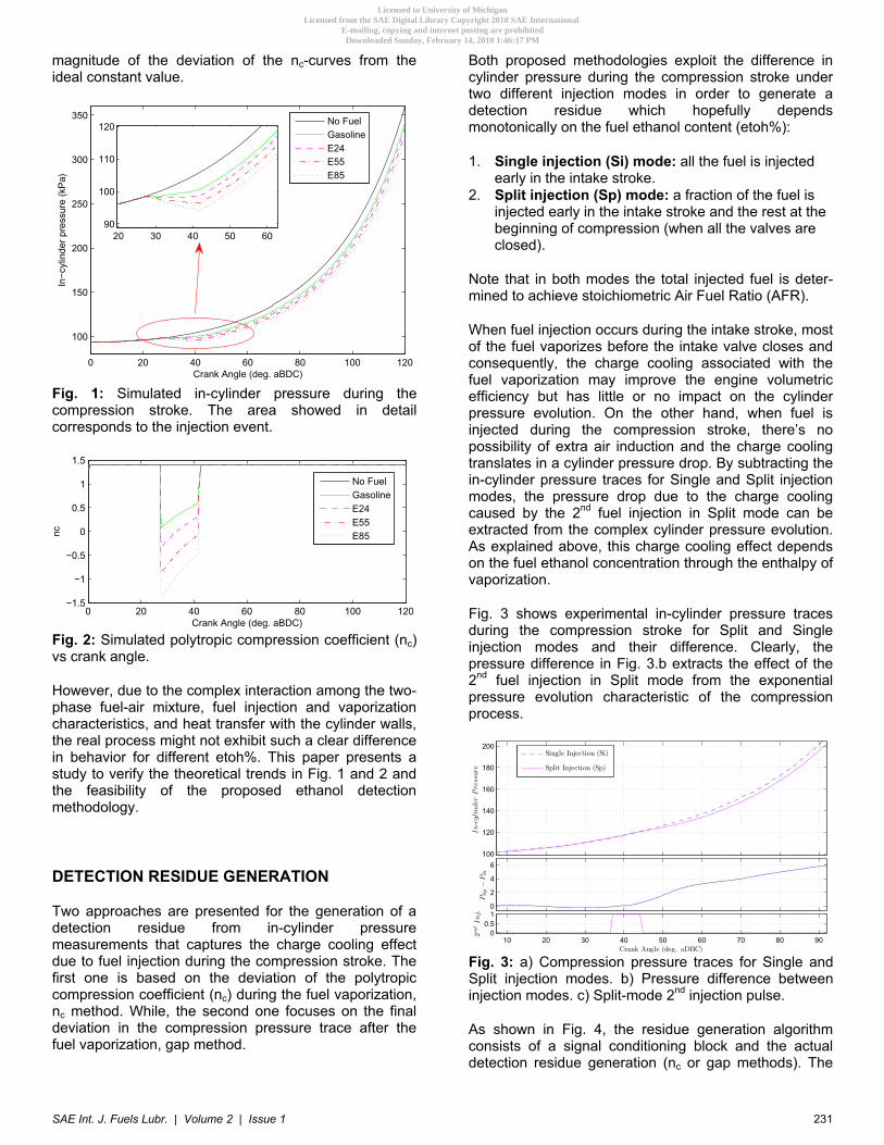
When fuel injection occurs during the intake stroke, most of the fuel vaporizes before the intake valve closes and consequently, the charge cooling associated with the fuel vaporization may improve the engine volumetric efficiency but has little or no impact on the cylinder pressure evolution. On the other hand, when fuel is injected during the compression stroke, there’s no possibility of extra air induction and the charge cooling translates in a cylinder pressure drop. By subtracting the in-cylinder pressure traces for Single and Split injection modes, the pressure drop due to the charge cooling caused by the 2nd fuel injection in Split mode can be extracted from the complex cylinder pressure evolution. As explained above, this charge cooling effect depends on the fuel ethanol concentration through the enthalpy of vaporization.

Fig. 3 shows experimental in-cylinder pressure traces during the compression stroke for Split and Single injection modes and their difference. Clearly, the pressure difference in Fig. 3.b extracts the effect of the 2nd fuel injection in Split mode from the exponential pressure evolution characteristic of the compression process.

10 20 30 40 50 60 70 80 90100

120

140

160

180

200

In-c

ylin

der

Pre

ssure

10 20 30 40 50 60 70 80 900

2

4

6

PS

p−

PS

i

10 20 30 40 50 60 70 80 900

0.51

2nd

Inj.

Crank Angle (deg. aDBC)

Single Injection (Si)

Split Injection (Sp)

Fig. 3: a) Compression pressure traces for Single and Split injection modes. b) Pressure difference between injection modes. c) Split-mode 2nd injection pulse.

As shown in Fig. 4, the residue generation algorithm consists of a signal conditioning block and the actual detection residue generation (nc or gap methods). The





algorithm can be combined in the future with an injection mode controller. The injection mode controller could determine when and how often Split injection mode is applied in order to achieve the desired estimation performance without compromising emissions or engine efficiency. This block was not implemented in this stage because the algorithm was executed off-line.

Fueling System

In-Cylinder High

Pressure Sensor

ENGINE

Single / Split

Residue

Signal Conditioning

Nor

mal

izat

ion

cylP

Injection Controller

Filte

ring

(FIR

)

Cyc

le

Aver

agin

g

1- nc method

2- gap method

Sp Inj.

Si Inj.

Residue Generation

Other enginevariables

Injection mode feedback

Tran

sfor

mat

ion

ohtEˆ

CONTROLLER

Residue Generation Algorithm

Fig. 4: High-level block diagram of the residue generation algorithm.

SIGNAL CONDITIONING - Regardless of the detection method, it is necessary to perform a pre-conditioning of the pressure measurements in order to eliminate several sources of error, as follows:

1. Engine conditions variations. 2. Cycle to cycle variations in the engine behavior. 3. Pressure sensor accuracy, noise, and quantization. 4. Disturbances and fast unmodeled dynamics.

The signal conditioning consists of 3 stages: normalization, cycle-average and filtering.

Normalization - Even small differences in the testing conditions can affect the process behavior and consequently, the algorithm results. In order to compare detection residues computed with data from different tests, a normalization of the measurements is required. For the current experimental data, a normalization only with respect to the load is being used which is computed using the intake manifold pressure, MAP, as shown in Eq. (3)

( ) ( ) 100

( ) = .

( )SoCp

SoIt

cyl SoCp SoItnorm

k

i k

P k k kP k

MAP i

� � �

� (3)

Where, Pcyl and MAP are vectors containing crank resolved cylinder and intake manifold pressure measurements respectively; kSoIt and kSoCp are the vector indexes corresponding to the start of the intake and compression strokes respectively; and 100 is a unit adjustment constant.

Cycle average - The cylinder pressure exhibits important cycle to cycle variations which are directly related to the stochastic nature of the combustion process. In order to

reduce this variability to an acceptable level and capture the charge cooling characteristics , several consecutive cycles need to be averaged.

=1

( ) = ( ).n

inorm

i

P k P k� (4)

For the results presented in this work an averaging of ten cycles (n=10) was used. The choice responds mainly to the available number of cycles at each tested condition.

Filtering - A filter is applied to the measurements to minimize two sources of error. The first one is measurement noise and quantization error introduced by sensors and the acquisition system. The second one, which for our purposes will be also considered noise, corresponds to disturbances inherent to the engine operation and unmodeled fast dynamics. One of the most important disturbances of this second type is seen in the pressure trace during the intake valve closure.

The filtering is realized by a 128th order finite impulse response (FIR) filter with a normalized cut of frequency ranging from 0.01 to 0.1

( 64) = ( ) ( )f FIRP k h k P k� � (5)

where: hFIR is the impulse response of the filter .

0 0.05 0.1 0.15 0.2 0.25−1500

−1000

−500

0

Normalized Frequency (×π rad/sample)

Pha

se(d

egre

es)

0 0.05 0.1 0.15 0.2 0.25

−100

−50

0

Mag

nitu

de(d

B)

Frequency Response

Cutoff Freq.: 0.01

Cutoff Freq.: 0.05

0 50 100 150 200

0

0.2

0.4

0.6

0.8

1

Sample number

Step

Res

pons

e

Input step

Output - Cutoff freq.: 0.05

Output - Cutoff freq.: 0.01

Fig. 5: Filter frequency and step responses

The cut of frequency selection responds to a trade-off between noise filtering capability and cylinder pressure





information loss, and the optimum value depends on the residue generation methodology.

FIR filters have linear phase through the entire pass-band which makes it possible to easily correct the delay introduced during filtering. Fig. 5 shows the filter characteristics for two different cutoff frequencies. A filtering example for the intake manifold absolute pressure (MAP) and the cylinder pressure is shown in Fig. 6. Notice that the sampling is performed every 0.5 CAdeg. which results in a speed-dependent sampling period in seconds. Therefore, the same digital filter has an effective cutoff frequency that varies proportionally with the speed, making unnecessary any adjustment of the filter for different speeds.

−40 −20 0 20 40 60

100

105

110

MA

P(k

Pa)

−40 −20 0 20 40 60

100

110

120

130

140

150

In-c

ylin

der

Pre

ssur

e(k

Pa)

−40 −20 0 20 40 600

0.5

1

2nd

Inj.


Measured data Filtered data

Fig. 6: Filtering Examples. a) MAP. b) In-cylinder pressure. c) Injection Pulse.

NC METHOD - The nc method is based on the polytropic compression coefficient. It exploits the transient effect on the polytropic coefficient resulting from the 2nd fuel injection in Split mode to generate the detection residue. The principle behind this approach was explained in the previous section and shown schematically in Fig. 2. A block diagram of the methodology is depicted in Fig. 7.

PolytropicCoefficientCalculation

Integration

injectionofStart __

Mean calculation

2

1

�

�

Split Inj.

nc method

Single Inj.

2

1

+S

-

Residue

Fig. 7: nc-method block diagram.

Fig. 8 illustrates the main signals involved in the method; points (1) and (2) in the block diagram. Fig. 8.a is the experimental equivalent to the simulated traces in Fig. 2. Clearly, the distinct features in Fig. 2 are smoothed out in Fig. 8.a mainly due to the filtering applied to the measurements and also to vaporization and heat transfer dynamics not included in the simplified model used to generate Fig. 2. Nevertheless, the fuel vaporization effect can be undoubtedly seen in Fig. 8.a. The area between the Single and Split traces in Fig. 8.a captures the fuel vaporization effect which should depend on the fuel ethanol content (etoh%). The final value of the curve in Fig. 8.b corresponds to the magnitude of the area.

107.5101948676.5654920.5

1.2

1.4

1.6

1.8

2

Pol

ytro

pic

Com

pre

ssio

nC

oeff.

107.5101948676.5654920.50

5

10

∫nc S

p−

nc S

i

107.5101948676.5654920.50

0.5

12n

dInj.




Fig. 8: Internal signals in nc method. a) Polytropic coefficient for Single (Si) and Split (Sp) modes (point 1). b) Area between the curves in (a) (point 2).

The nc method consists of a sequence of operations as illustrated in Fig. 7 and described in the following paragraphs.

Polytropic Coefficient Calculation - The polytropic compression coefficient, nc, can be computed by:

( )

= .( )

cylc

cyl

log Pn

log V

��

(6)

In order to overcome the noise problems associated with the differentiation in Eq. 6 , a linear regression on a moving window is performed instead. That is, the polytropic compression coefficient at a point x is the slope of a line fitted on [log(Pcyl),log(Vcyl)] in a window centered at x The complete calculation involves a sequence of steps:

First, a uniformly sampled set of vectors for [log(Pcyl),log(Vcyl)] is generated:

� �ˆ ˆ( ) = ( )cyl logVlogV k min log V k� �� (7)

� �� ˆ = / ( ) < ( )cylk i N logV i max log V�





� � � ��

� �

ˆ ˆ( ) ( )ˆ ˆ( ) = ( ( ))

ˆ ˆ( ) ( )

ˆ ˆ( ) ( )

cyl b cyl a

cyl a

cyl b cyl a

cyl a

log P k log P klogP k log P k

log V k log V k

logV k log V k

��

�

� ��

(8)

� �� ˆ ˆ= / ( ) < ( )a i cylk max i N log V i logV k�

� �� ˆ ˆ= / ( ) > ( ) .b i cylk min i N log V i logV k�

Then, a linear regression on a window of width 2 W� is computed:

� �ˆˆ ˆ= ( ) / < <W

klogV logV i k W i k W� � � � (9)

� �ˆˆ ˆ= ( ) / < <W

klogP logP i k W i k W� � � � (10)

� � 1

ˆ ˆ

ˆ ˆ

= [ 1] [ 1]

[ 1]

W T Wk k

W T Wk k

mlogV logV

b

logV logP

��

� ��

(11)

ˆ( ) = .cn k m� (12)

Finally, a 0.5CAdeg-sampled nc vector is generated:

� �

( ) ( )( ) = ( )

( ) ( )

( ) ( )

c b c ac c a

b a

cyl a

n k n kn k n k

logV k logV k

V k logV k

� ��

� � (13)

= {1,2, ,2 }k EoCp� (14)

� �� = / ( ) < ( )a i cylk max i N logV i log V i� (15)

� �� = / ( ) > ( ) ,b i cylk min i N logV k log V i� (16)

where EoCp is the end of compression and in the current implementation is defined as 5 CAdeg. before ignition.

Integration - It is clear from Fig. 8.a that the fuel vaporization effect is not concentrated only during the injection period as suggested in Fig. 2. Due to the filtering and vaporization and heat transfer dynamics, the charge cooling spreads out before and after the injection event. In order to capture the whole effect, the area in between the polytropic coefficients for the different injection modes, Anc,dif is computed according to Eq. (17)

2

, ( ) = ( ) ( ),SoIj

kSi Sp

nc dif c ci k

A k n i n i

�� (17)

where, SoIj2 is the start of the 2nd fuel injection.

The integration also attenuates the effect of disturbances and noise present in the experimental data. When the injection transient vanishes, the integration reaches a steady condition with a mean value that should be proportional to the total charge cooling and consequently the etoh%.

Mean calculation - The final value of Anc,dif(k) oscillates due to disturbances not related with the cooling process. In order to reduce the detection variability, the mean value of Anc,dif(k) is computed during the last part of the compression stroke to obtain the residue, Residuenc

145

105

,

145 105

( )

= ,

SoCp

SoCp

k

nc difi k

ncSoCp SoCp

A i

Residuek k

� �

� �

� � � ��

� (18)

where, SoCp is the start of the compression stroke and the limits for the mean calculation are currently set in [105,145] CAdeg, but this interval is tunable.

GAP METHOD - When fuel is injected during the compression period, the cylinder charge is cooled down changing the pressure evolution throughout the rest of the compression stroke as shown schematically in Fig. 1. The gap method is based on the final pressure difference between Single and Split injection modes, caused by the 2nd fuel injection. Fig. 9 shows a block diagram of the algorithm.

Mean calculation

2

1

�

�

Split Inj.

gap method

DifferenceZeroing Log( )

+S

-

1

2

Residue

Single Inj.

Fig. 9: Gap-method block diagram.

Fig. 10.a shows the logarithm of the compression pressure traces for Single and Split injection modes. The cylinder pressure for both injection modes evolve together before the 2nd fuel injection. Then, during the fuel vaporization event, the in-cylinder pressure for the Split mode drops, and finally both traces continue parallel to each other. This result agrees with the nc method which indicates that the polytropic compression coefficient for both injection modes is the same before and after the 2nd fuel injection and vaporization transient. Fig. 10.b shows the difference between both traces in (a). The final value of the difference reaches a steady state which depends on the total charge cooling due to the 2nd injection.





90.58681.576.5716557.5493820.5

4.7

4.8

4.9

5

5.1

5.2

5.3L

ogof

In-c

ylin

der

Pre

ssure

90.58681.576.5716557.5493820.5

0

0.01

0.02

0.03

log(

PS

p)−

log(

PS

i)

90.58681.576.5716557.5493820.50

0.5

1

2nd

Inj.




Fig. 10: Internal signals in gap method. a) log(P) for Single (Si) and Split (Sp) modes (point 1) b) Difference between the signals in a) (point 2).

As depicted in Fig. 9 the gap method consists of sequence of steps described in the following paragraphs.

Difference Zeroing - Unlike the nc approach, the gap method is very sensitive to offset errors which translate directly to the computed residue. In order to account for any measurement offset, the mean difference between the Single and Split traces before the start of the 2nd injection is set to zero, as indicated in Eq. (19) and (20). This is based on the fact that under similar engine conditions the first part of both traces should be identical and any difference must be due to pegging errors. Pegging is an important source of error with in-cylinder pressure transducers.

2

02

( ) ( )1

( ) = ( )2

SoIj

SoCp

kSp Si

i kSi Sif

SoIj SoCp

P i P i

P k P kk k

��

�

� ��

� (19)

2

02

( ) ( )1

( ) = ( ) .2

SoIj

SoCp

kSp Si

i kSp Spf

SoIj SoCp

P i P i

P k P kk k

��

�

� ��

� (20)

Where, kSoIj2 and kSoCp are the data vector indexes corresponding to the start of the 2nd injection and the compression stroke respectively, and � accounts for the spread of the charge cooling due to the filtering and vaporization dynamics.

Then, the pressure difference between Split and Single modes, Gap(k), is computed by Eq. (21)

0 0( ) = log( ( )) log( ( )).Si SpGap k P k P k� (21)

Mean calculation - The mean calculation has the same foundations as for the nc method. The gap-method residue, Residuegap, is computed according to Eq. (22)

145

105

145 105

( )

= .

SoCp

SoCp

k

i k

gapSoCp SoCp

Gap i

Residuek k

� �

� �

� � � ��

� (22)

EXPERIMENTAL VALIDATION

The proposed detection concept and methodologies were validated with dynamometer data. Tests with Single and Split injection were performed on a General Motors 2.0L DI Turbo LNF engine. Kistler 6125B cylinder pressure sensors were installed in all the cylinders. The engine specifications are listed in Table 2. Experimental data was collected for fuels: E0, E40, E55, E70 and E85.

Number of cylinders 4 Cylinder displacement 500 cm3/cyl. Compression ratio 9.25:1 Injectors Qstat 22.5 cc @ 100 bar Fuel pump pressure up to 150 bar Turbo max boost 2.3 bar

Table 2: Engine specifications

For each fuel blend, the engine was tested at five different speeds and loads listed in Table 3. The reported loads correspond to the mass air flow (MAF) setpoint at the dynamometer. The selected operating points are common engine conditions based on typical driving cycles and MBT spark timing was used for all the tested conditions and fuels.

Point Speed (RPM)

Load (kg/hr)

1500_80 1500 80 2000_100 2000 100 2000_150 2000 150 2500_130 2000 130 2500_170 2000 170

Table 3: Tested operating points

Variable Description Value

IVO0 Intake valve opening 30 CAdeg BTDC

EVC0 Exhaust valve closure 20 CAdeg ATDC

PFuel,0 Fuel rail pressure 6 MPa

SpRatio0 Split Injection ratio 50/50 (%)

SoIj1, SoIj Start of 1st Injection Gasoline Cal.

EoIj2 End of 2nd Injection 40 CAdeg aBDC

SoIg Ignition Timing MBT

0 AFR/AFRstoichiometric 1

Table 4: Nominal test conditions

Table 4 summarizes the nominal conditions for the tests. Both Single and Split injection modes were run at stoichiometric AFR and at each test point all the





operating conditions were kept constant with exception of the fuel injection pattern. The Start of 1st Injection (SoIj1) in Split mode was the same as the Start of Injection (SoIj) for Single mode and the values used for all fuel blends were the ones defined by the standard engine calibration for gasoline. The End of 2nd Injection (EoIj2) in Split mode was fixed at 40 CAdeg after BDC to ensure the intake valve is closed during the injection while allowing the sufficient charge mixing necessary for a good combustion. The injection split ratio of 50% used in Split mode corresponds to a tradeoff between combustion quality, minimum injection timing and detection sensitivity, but the optimization of this value was left for future work.

Furthermore, in order to obtain a deeper understanding of the fuel vaporization process, tests with different exhaust valve timings and fuel rail pressures were performed. Table 5 lists the variations on the nominal conditions performed for the different operation points.

Point PFuel,1 PFuel,2 EVC1 1500 80 2500 130 10 MPa 15 MPa 40 CAdeg ATDC2500 170

2000 100 12 MPa - 40 CAdeg ATDC2000 150

Table 5: Variations on nominal test conditions

The algorithms were executed with cylinder pressure data collected for cylinder 4 and using a filter cutoff frequency of 0.05 for the gap method and 0.01 for the nc method. A cutoff frequency of 0.05 guarantees no distortion on the pressure evolution, while 0.01 smooths out some details but at the same time attenuates disturbances and noise which deteriorate the nc-method performance significantly. Detection residues were generated with both methods using and averaging of 10 cycles which given the available data allowed the computation of 7 residues for each condition and fuel blend. The averages of the 7 residues obtained for each blend were also computed. Note that, there are two levels of averaging: cycle and residue. The combination of both determines the detection time and accuracy. A detailed study with more experimental data needs to be performed to determine the optimal combination of cycle and residue averaging.

Fig. 11 shows gap-method residues for all the tested operating points under nominal conditions. The +'s and x's correspond to single residues computed from 20 consecutive cycles, while the o's and �'s are the respective seven-residues averages. The lines are least squared linear regressions on the averaged values. The experimental results show a monotonic and consistent correlation between the residues and the fuel ethanol content (etoh%) in the majority of the cases. At 2000 RPM and 2500 RPM, the algorithm output is approximately linear with respect to the etoh% for all

blends (E0-E85); while at 1500 RPM a nonlinear behavior can be observed for high-ethanol blends (E85).

0 10 20 30 40 50 60 70 80 900.015

0.02

0.025

0.03

0.035

Det

ecti

onR

esid

ue(g

apM

ET

HO

D)

Real Etoh%

2500 170 - Single2500 170 - Average2500 130 - Single2500 130 - Average

(a) [2500 RPM, 130 and 170 kg/hr.]

0 10 20 30 40 50 60 70 80 900.015

0.02

0.025

0.03

0.035

Det

ecti

onR

esid

ue(g

apM

ET

HO

D)

Real Etoh%


(b) [2000 RPM, 100 and 150 kg/hr.]

0 10 20 30 40 50 60 70 80 900.015

0.02

0.025

0.03

0.035

Det

ecti

onR

esid

ue(g

apM

ET

HO

D)

Real Etoh%

1500 80 - Single1500 80 - Average

(c) [1500 RPM, 80 kg/hr]

Fig. 11: Gap-method residues for nominal conditions.

Results for the nc method are shown in Fig. 12. This approach has a higher variability which is a result of the derivative involved in the polytropic coefficient concept. At 1500 RPM, the nc-method results are acceptable and the variability is comparable to the gap method. However, the variability increases with engine speed and, above 2000 RPM, the influence of engine disturbances, such as valve closure, is excessively





large. Therefore, the rest of the analysis will concentrate on the gap method.

0 10 20 30 40 50 60 70 80 904

6

8

10

12

14

16

Det

ecti

onR

esid

ue(n

cM

ET

HO

D)

Real Etoh%


(a) [2000 RPM, 100 and 150 kg/hr.]

0 10 20 30 40 50 60 70 80 904

6

8

10

12

14

16

Det

ecti

onR

esid

ue(n

cM

ET

HO

D)

Real Etoh%

1500 80 - Single1500 80 - Average

(b) [1500 RPM, 80 kg/hr.]

Fig. 12: nc-method residues for nominal conditions.

Fig. 13 and 14 illustrate the effects of fuel rail pressure on gap-method residues; only the seven-residues averages for each fuel blend are shown . It can be observed that the residues vary nonlinearly with the fuel rail pressure for different ethanol contents. For E0 (gasoline), the rail pressure has little effect on the algorithm output and at high loads, a slight reverse effect can even be observed; i.e. the residue varies inversely to the fuel rail pressure. As etoh% increases, the fuel rail pressure has a stronger effect on the algorithm output. These results suggest that a higher fuel rail pressure significantly improves the vaporization of ethanol. At high loads, a saturation effect seems to appear in the algorithm output as can be seen at 2500 RPM - 170 kg/hr. The same trends are also observed at other engine speeds.

Fig. 15 illustrates the effect of changes in the exhaust valve timing; only the 7-residues averages for each fuel blend are shown. Delaying the exhaust valve closure (EVC) modifies the internal exhaust gas recirculation (EGR) amount, hence, the cylinder charge temperature

0 10 20 30 40 50 60 70 80 900.015

0.02

0.025

0.03

0.035

0.04

Det

ecti

onR

esid

ue(g

apM

ET

HO

D)

Real Etoh%

Pfuel = 6.3MPaPfuel = 10.0MPaPfuel = 15.0MPa

Fig. 13: Gap-method residues for different fuel rail pressures at 2500 RPM - 130 kg/hr.

0 10 20 30 40 50 60 70 80 900.015

0.02

0.025

0.03

0.035

0.04

Det

ecti

onR

esid

ue(g

apM

ET

HO

D)

Real Etoh%

Pfuel = 7.2MPaPfuel = 9.9MPaPfuel = 14.9MPa

Fig. 14: Gap-method residues for different fuel rail pressures at 2500 RPM - 170 kg/hr.

at IVC which is expected to modify the fuel vaporization characteristics. In order to estimate the EGR level at each operating point and condition, energy balance at intake valve closure (IVC) is used [21].

0 10 20 30 40 50 60 70 80 900.015

0.02

0.025

0.03

0.035

Det

ecti

onR

esid

ue(g

apM

ET

HO

D)

Real Etoh%

2000 150 / EVC0

2000 150 / EVC1

2000 100 / EVC0

2000 100 / EVC1

Fig. 15: Gap-method residues for different exhaust valves timings (EVT) at 2000 RPM





2000 150 2000 100 EVC0 EVC1 EVC0 EVC1 EVC (deg) 20 38 24 37 MAF (kg/hr) 150 154 101 99 Avg. EGR (%) 2.8 2 10.5 11.5

Table 6: Average EGR% for 2000 RPM and nominal (EVC0) and delayed (EVC1) exhaust valve timings.

Table 6 shows the estimated EGR percentages for the conditions plotted in Fig. 15. At low loads the EGR amount follows the valve overlap variations, while at high loads the dependence is weaker and even a decrease in EGR can be observed for increased valve overlap. The detection residues in Fig. 15 follow the trends observed in the estimated EGR amounts. Large EGR percentages at the low load conditions (2000_100) agree with high detection residues. Besides, at low load, an increase in the overlap (condition EVC1) is followed by an increased in both, the EGR level and the detection residues. At high load, the EGR level does not increase for increased overlap (EVC1) which agrees with the small change observed in the residues.

0 10 20 30 40 50 60 70 80 90−20

0

20

40

60

80

100

Est

imat

edE

toh%

(gap

ME

TH

OD

)

Real Etoh%

2500 1702500 130

(a) [2500 RPM - 170 and 130 kg/hr.]

0 10 20 30 40 50 60 70 80 90−20

0

20

40

60

80

100

Est

imat

edE

toh%

(gap

ME

TH

OD

)

Real Etoh%

2000 1502000 100

(b) [2000 RPM - 150 and 100 kg/hr.]

Fig. 16: Gap-method ethanol estimation results using an affine transformation for 2500RPM - 170 and 130Kg/hr, 2000RPM - 150 and 100Kg/hr .

In order to obtain a rough estimation of the possible achievable ethanol detection accuracy, the residues were converted to ethanol percentage using an affine transformation. For each condition, a transformation was computed using a linear regression on the residues versus the known ethanol percentage in the fuel. Although, a nonlinear instead of an affine transformation might be needed for the best detection accuracy, the affine relation provides a clear idea of the magnitude of the nonlinearities in the process. Fig. 16 shows averaged ethanol detection results together with the associated single estimations variability for 2000 RPM and 2500 RPM. The averages are computed using 7 consecutive ethanol estimations and each single estimation is based on 20 engine cycles.

The time required to generate the residues is inversely proportional to the engine speed. Table 7 illustrates the estimation time for the conditions plotted in Fig. 16 and Table 8 summarizes the averaged etoh% estimation values together with their absolute errors.

Single residue Average (based on 20 cycles) (7 residues) 2500 RPM 0.96 Sec 6.72 Sec 2000 RPM 1.20 Sec 8.40 Sec

Table 7: Ethanol estimation time for 2000 RPM and 2500 RPM.

E0 E40 E55 E70 E85 2500_170 Avg. etoh% 1.71 35.35 56.34 65.52 84.23Error 1.71 -4.65 3.04 -2.23 2.13 2500_130 Avg. etoh% -3.14 41.02 59.73 64.28 78.76Error -3.14 2.53 6.73 -3.22 -2.90 2000_150 Avg. etoh% -0.34 40.75 49.71 69.56 83.76Error -0.34 2.49 -3.94 2.06 -0.28 2000_100 Avg. etoh% -5.77 45.51 59.02 68.60 76.82Error -5.77 7.49 4.20 1.11 -7.04

Table 8: Ethanol estimation results using affine transformations for 2000 RPM and 2500 RPM.

The large variability observed at 2000 RPM - 150 kg/hr for E85 in Fig. 11.b and 16.b may be a result of cycle to cycle combustion variations. These variations in the combustion process affect the cylinder temperature and pressure after combustion which in turn modify the internal exhaust gas recirculation (EGR) amount at the next cycle. Finally, the vaporization process during the compression stroke and consequently the detection residues depend on the cylinder charge characteristics and therefore are sensitive to the combustion variability. In order to understand the detection residue variability and other trends observed in the experimental results, a physics-based model is being developed. The model is





deterministic and simulates the cylinder pressure trace during the compression stroke based on an estimated cylinder charge, composition and temperature, at intake valve closure (IVC)[21]. Energy and mass conservation [19, 22] along with a multi-component fuel vaporization model [23, 24, 25, 26, 27] are then utilized to model the intake-compression process.

The detection algorithm is applied on the numerically simulated cylinder pressure traces and the detection residues based on the gap-method are calculated. Note here that variability can only be introduced in the simulations by the estimated charge characteristics through the model inputs listed in Table 9.

Measurement Symbol Exhaust temperature TEGIntake temperature Ta

Mass of fresh air (MAF) ma

Intake cylinder pressure Pcyl,real

Injected fuel mass mfl,inj

Injection pulse Siginj

Ignition pulse Sigign

Exhaust valve timing EVTIntake valve timing IVTFuel ethanol content ereal

Table 9: Measurements used as inputs for the simulation

Fig. 17 shows the residues generated from simulated pressure traces for 2000 RPM - 150 kg/hr. It can be observed that the residue variability obtained from the simulations is consistent with the experimental results in Fig. 11.b.

0 10 20 30 40 50 60 70 80 900.015

0.02

0.025

0.03

0.035

Sim

ulat

edD

etec

tion

Res

idue

(gap

ME

TH

OD

)

Real Etoh%

2000 150 - Single2000 150 - Average

Fig. 17: Gap-method residues for 2000 RPM - 150 kg/hr computed from simulated pressure traces.

Fig. 18 and 19 show the variability in the estimated EGR mass and cylinder charge temperature corresponding to the simulations in Fig. 17.

0 10 20 30 40 50 60 70 80 904

4.5

5

5.5

6

6.5

7

7.5x 10

−6

Real etoh%

EG

Rm

ass

diffe

renc

ebe

twee

nSi

and

Sp

Fig. 18: Difference in estimated EGR mass between Single and Split injection modes for different fuel blends.

0 10 20 30 40 50 60 70 80 90−6.5

−6

−5.5

−5

−4.5

−4

−3.5

Real etoh%

IVC

char

gete

mp.

diff.

betw

een

Sian

dSp

Fig. 19: Difference in estimated cylinder charge temperature between Single and Split injection modes for different fuel blends.

The variability in the cylinder charge estimations must be a consequence of the cycle to cycle combustion variations that propagate into the model through the measured intake and exhaust pressures and temperatures. Besides, the simulated residues in Fig. 17 follow the variability in the charge estimations which indicates that the residue variability to some extent can be captured by the model.

These preliminary results suggest that more robust detection with smaller estimation errors could be obtained by means of a model-based detection scheme with an appropriate model, provided that accurate measurements or estimations of the model inputs listed in Table 9 are available on-line.

CONCLUSION

The feasibility of a novel approach for ethanol detection in engines equipped with direct injection was presented. The methodology is based on in-cylinder pressure measurements during the compression stroke, and exploits the different charge cooling effect between gasoline and ethanol. A data-driven algorithm was introduced to validate the detection concept with





dynamometer data. Two different methodologies were developed; the nc method is based on deviations in the polytropic compression coefficient, while the gap method focuses on final deviations in the compression pressure trace. Both approaches compare the compression pressure traces under Single and Split injection modes to generate a residue that captures the charge cooling effect. Experiments were performed at different speeds, loads, fuel rail pressures and exhaust valve timings with ethanol-gasoline blends ranging from 0% to 85% of ethanol (E0 to E85).

The gap method outperforms the nc approach due to its lower sensitivity to noise and disturbances, such as, valve closure. The experimental results show a monotonic and consistent correlation between the residues and the fuel ethanol content (etoh%) in the majority of the cases. At 2000 RPM and 2500 RPM, the algorithm output is approximately an affine function of etoh% for all blends (E0-E85); while, at 1500 RPM a nonlinear behavior can be observed for high-ethanol blends (E85). The experimentally determined correlations between residues and etoh% for different loads and speeds could be stored as a look-up table in the vehicle micro-controller for on-board ethanol estimation.

Work currently in progress includes the development of a model to capture the experimental trends observed for different engine operating conditions; such as, speed, load, fuel rail pressure, valve timing, intake and exhaust temperature and pressure. Once the model is calibrated, it will be used for the development of a model-based ethanol detection algorithm able to run in real-time under dynamic engine conditions without resort to complex look-up tables that are solely determined from dynamometer experiments.

ACKNOWLEDGMENTS

The present work has been performed within the scope of the "Optimally Controlled Flexible Fuel Powertrain System" project, sponsored by the Department of Energy (DOE). The authors gratefully acknowledge: the DOE for the financial support; Michael Caruso for assisting with the administrative and financial aspects of the project; Julien Vanier for modifying the engine control unit (ECU) code to execute the required tests and his support throughout the experiments; Mark Christie and Nicholas Fortino for providing some of the early dynamometer data.

REFERENCES

1. Nakata K., Utsumi S., Ota A., Kawatake K., Kawai T., and Tsunooka T., The effect of ethanol fuel on spark ignition engine. SAE World Congress, 2006-01-3380, 2006.

2. Cowart J. S., Boruta W. E., Dalton J. D., Dona R. F., Rivard F. L., Furby R. S., Piontkowski J. A., Seiter R.

E., and Takai R. M., Powertrain development of the 1996 ford flexible fuel taurus. SAE World Congress, 952751, 1995.

3. Castro Adriano C., Koster Carlos H., and Franieck Erwin K., Flexible ethanol otto engine, management system. SAE World Congress, 942400, 1994.

4. Volpato O., Theunissen F., and Mazara R., Engine management for flex fuel plus compressed natural gas vehicles. SAE World Congress, 2005-01-3777, 2005.

5. Seitz G. L., et al, “Method of determining the composition of fuel in a flexible fueled vehicle with an O2 sensor”, US Patent 5850824, December 22, 1998.

6. Rotramel W. D., et al, “Method for determining the composition of fuel in a flexible fuel vehicle without an O2 sensor”, US Patent 5950599, September 14, 1999.

7. Theunissen F., Percent ethanol estimation on sensorless multi-fuel systems; advantages and limitations. SAE World Congress, 2003-01-3562, 2003.

8. Moote R. K., Huff S., Joyce M., Krausman H. W., and Seitz G. L., “Method of determining ethanol thresholds in a flexible fuel vehicle”, US Patent 5868117, February 09, 1999.

9. Kennie J., et al, “Method of triggering a determination of the composition of fuel in a flexible fueled vehicle”, US Patent 6041278, March 21, 2000.

10. Washino S., and Ohkubo S., “Fuel properties detecting apparatus for an internal combustion engine”, US Patent 4905649, March 6, 1990.

11. Mitsumoto H., “System and method for controlling ignition timing for internal combustion engine in which alcohol is mixed with gasoline”, US Patent 5050555, September 24, 1991.

12. Abo T.,Satoh H., and Takahashi N., “Fuel monitoring arrangement for automotive internal combustion engine control system”, US Patent 4920494, April 24, 1990.

13. Powell J., (Jun 1993). Engine control using cylinder pressure: Past, present, and future. ASME Journal of dynamic Systems, Measurement, and Control, 115.

14. Gilkey J. and Powell J., (Dec 1985). Fuel-air ratio determination from cylinder pressure time histories. ASME Journal of dynamic Systems, Measurement, and Control, 107.

15. Gassenfeit E. and Powell J., Algorithms for air-fuel ratio estimation using internal combustion engine cylinder pressure. SAE World Congress, 890300, 1989.

16. Patrick R. and Powell J., A technique for real-time estimation of air-fuel ratio using molecular weight ratio. SAE World Congress, 900260, 1990.

17. Sellnau M., Matekunas F., Battiston P., Chang C., and Lancaster D., Cylinder-pressure-based engine control using pressure-ratio-management and low-





cost nonintrusive cylinder pressure sensors. SAE World Congress, 2000-01-0932, 2000.

18. Bromberg L., Cohn D., and Heywood J., “Optimized fuel management system for direct injection ethanol enhancement of gasoline engines”, US Patent No. 7,225,787 B2, June 5, 2007.

19. Fundamentals of thermodynamics, Sontag R., Borgnakke C., and Wylen G. Van. John Wiley & Sons Inc, 6th edition, 2003.

20. Rausen D., Kang J-M., Eng J. A., Kuo T-W., and Stefanopoulou A., (Sep 2005). A mean-value model for control of homogeneous charge compression ignition (HCCI) engines. ASME Journal of dynamic systems, measurements and control, 127.

21. Oberg P., and Erikssons L., Control oriented modeling of the gas exchange process on variable cam timing engines. SAE World Congress, 2006-01-0660, 2006.

22. Internal Combustion engines fundamentals, Heywood J. B. McGraw Hill, 2nd edition, 1988.

23. Combustion and Mass Transfer, Spalding D. B. Pergamon Press, 1st edition, 1979.

24. Locatelli M., Onder C. H., and Geering H. P., An easily tunable wall-wetting model for PFI engines. SAE World Congress, 2004-01-1461, 2004.

25. Batteh J. and Curtis E., Modeling transient fuel effect with alternative fuels. SAE World Congress, 2005-01-1127, 2005.

26. Senda J., Higaki T., Sagane Y., Fujimoto H., Takagi Y., and Adachi M., Modeling and measurement on evaporation process of multicomponent fuels. SAE World Congress, 2004-01-1461, 2004.

27. Barata J., (Apr 2008). Modeling of biofuel droplets dispersion and evaporation. Journal of Renewable Energy, 33(4).





Documents

Ethanol Detection in Flex-Fuel Direct Injection Engines ...annastef/papers_FFV/Oliverio_SAE_2009-01... · Ethanol detection could also ... overlap with the EGO-based method because