Estimation of Vehicle Attitude, Acceleration and Angular

Sensors 2021, 21, 1282. https://doi.org/10.3390/s21041282 www.mdpi.com/journal/sensors

Article

Estimation of Vehicle Attitude, Acceleration and Angular

Velocity Using Convolutional Neural Network and Dual

Extended Kalman Filter

Minseok Ok 1, Sungsuk Ok 2 and Jahng Hyon Park 1,*

1 Department of Automotive Electronics & Control Engineering, Hanyang University, Seoul 04763, Korea;

[email protected] 2 Autonomous Driving Center, Hyundai Motor Company R&D Division, Seoul 06182, Korea;

[email protected]

* Correspondence: [email protected]; Tel.: +82-2-2220-0448

Abstract: The acceleration of a vehicle is important information in vehicle states. The vehicle accel-

eration is measured by an inertial measurement unit (IMU). However, gravity affects the IMU when

there is a transition in vehicle attitude; thus, the IMU produces an incorrect signal output. Therefore,

vehicle attitude information is essential for obtaining correct acceleration information. This paper

proposes a convolutional neural network (CNN) for attitude estimation. Using sequential data of a

vehicle’s chassis sensor signal, the roll and pitch angles of a vehicle can be estimated without using

a high-cost sensor such as a global positioning system or a six-dimensional IMU. This paper also

proposes a dual-extended Kalman filter (DEKF), which can accurately estimate acceleration/angular

velocity based on the estimated roll/pitch information. The proposed method is validated by real-

car experiment data and CarSim, a vehicle simulator. It accurately estimates the attitude estimation

with limited sensors, and the exact acceleration/angular velocity is estimated considering the roll

and pitch angle with de-noising effect. In addition, the DEKF can improve the modeling accuracy

and can estimate the roll and pitch rates.

Keywords: sensor fusion; state estimation; vehicle dynamics; convolutional neural network; dual

extended Kalman filter; vehicle roll and pitch angle; vehicle acceleration and angular velocity

1. Introduction

In recent decades, the vehicle controller has been developed significantly for stability

and user convenience. Typically, the electronic stability controller (ESC) or active roll sta-

bilization (ARS) are used for ensuring vehicle stability in chassis controller, adaptive

cruise control (ACC), or lane keeping system (LKS) as well as for ensuring convenience in

advanced driver assistant system (ADAS). To improve the performance of these control-

lers, vehicle states must be estimated with a high accuracy. The commonly required and

important state information of aforementioned controllers are acceleration and angular

velocity. In a vehicle, the inertial measure unit (IMU) measures the acceleration and an-

gular velocity using an inertial force. However, if a transition in attitude (roll and pitch)

occurs, the gravitational force is reflected in the sensor value. The IMU cannot distinguish

between gravitational force and inertial forces; therefore, a change in the attitude of the

vehicle causes a fatal error in the IMU.

Several studies have been conducted to overcome the errors in these accelerometers

and to estimate the exact state of the vehicle. In [1,2], the adaptive Kalman filter was de-

signed to minimize the effect of the accelerometer offset errors. In addition, the Kalman

filter was used to estimate the accelerometer offset and vehicle velocity [3–5]. However,

Citation: Ok, M.; Ok, S.; Park, J.H.

Estimation of Vehicle Attitude,

Acceleration and Angular Velocity

Using Convolutional Neural

Network and Dual Extended Kal-

man Filter. Sensors 2021, 21, 1282.

https://doi.org/10.3390/s21041282

Academic Editor: Maria Jesús

López Boada

Received: 14 January 2021

Accepted: 8 February 2021

Published: 11 February 2021

Publisher’s Note: MDPI stays neu-

tral with regard to jurisdictional

claims in published maps and insti-

tutional affiliations.

Copyright: © 2021 by the authors.

Licensee MDPI, Basel, Switzerland.

This article is an open access article

distributed under the terms and con-

ditions of the Creative Commons At-

tribution (CC BY) license (http://cre-

ativecommons.org/licenses/by/4.0/).

Sensors 2021, 21, 1282 2 of 22

the accuracy of estimating vehicle states was limited because of a lack of information of

the vehicle attitude.

Several studies have been conducted to estimate the accurate vehicle attitude in var-

ious ways. Using IMU or GPS or vehicle dynamics, researchers tried to estimate the vehi-

cle roll and pitch angle. In addition, due to the recent developments in artificial intelli-

gence and neural networks, data-driven estimators have been used for state estimation

[6]. These estimators have the advantage of having high accuracy by training the data

directly in situations where accurate mathematical modeling is difficult. The literature re-

view is discussed separately in Section 2.

This paper proposes a novel vehicle attitude estimator using a convolutional neural

network (CNN), based on the advantages of a data-driven estimator. Figure 1 shows the

architecture of the proposed algorithm. First, we select the features based on vehicle roll

and pitch dynamics, importance judgment and sensor usability. By using the selected fea-

tures sequentially [7], the three-dimensional IMU and vehicle sensor build a CNN-based

regression model that can estimate the vehicle roll and pitch angles without GPS. Moreo-

ver, a dual extended Kalman filter (DEKF) is designed to estimate the exact accelera-

tion/angular velocity based on the estimated roll and pitch angles with removing the effect

of gravitational force. The proposed model is based on the sprung mass six-degree-of-

freedom (6-DOF) model and increases the modeling accuracy while estimating the tire

cornering stiffness simultaneously. The performance of the proposed algorithm was ver-

ified using real car experiment data and MATLAB/Simulink with CarSim, a vehicle sim-

ulator. A CNN conducted training and verification using data collected from various driv-

ing conditions as an experimental vehicle with RT-3002 which is a high-accuracy GPS-

inertial navigation system (INS) from Oxford Technical Solutions Ltd. The performance

of the DEKF was verified with a scenario in which postural changes occur using CarSim

and MATLAB/Simulink.

Figure 1. Architecture overview.

The remainder of this paper is organized as follows. Section 2 describes the related

literature review. Section 3 explains the methodology including neural network and

DEKF. Section 4 describes the results of performance verification. Section 5 summarizes

the study and contributions.

2. Literature Review

Several studies have been conducted to estimate the accurate vehicle attitude in var-

ious ways. In [8], authors proposed an observer which can estimate the land vehicle’s roll

and pitch by using an IMU and the kinematics model. Also, the adaptive Kalman filter

was proposed based on IMU aided by vehicle dynamics [9]. However, these methods have

a low accuracy in dynamic situations. This problem was attempted to be solved in [10–

Sensors 2021, 21, 1282 3 of 22

13], based on the Kalman filter by compensating for the external acceleration that inter-

fered with the estimation of the attitude, but the accuracy was limit.

Therefore, many researchers have proposed sensor fusion method using not only

IMU but fusion with global positioning system (GPS). Representatively, the method in

which IMU and GPS fusion with Kalman filter [14–16] or sliding mode observer [17] can

be used. These methods can increase the accuracy, but they require high-cost sensors such

as GPS and are highly affected by GPS performance.

Accordingly, vehicle attitude estimator studies were conducted without the use of

GPS, based on the characteristics of the vehicle dynamics. Using vehicle roll dynamics, a

dynamic observer design based on a reliable rollover index [18] was proposed. Also, the

Kalman filter [19] and the robust observer [20] based on vehicle roll dynamics which esti-

mate roll angle were proposed. Alternatively, using lateral dynamics, the research which

estimate road bank angle [21-22] was proposed. However, these methods exhibited lim-

ited accuracy in transient situations. A method for estimating both roll and pitch attitudes

using a six-dimensional IMU and bicycle model [23-24] was also studied. These methods

exhibited a high accuracy, but they have a short validation range and required hard-to-

get data such as six-dimensional IMU.

Several recent studies have also been conducted to estimate the vehicle roll and pitch

angle using neural network. In [25–27], the vehicle roll angle estimation method using

sensor fusion with a neural network and Kalman filter was proposed. Furthermore, a ve-

hicle roll and road bank angle estimation method based on a deep neural network was

introduced [28]. However, the pitch attitudes were not estimated, and the six-dimensional

IMU data such as roll rate or vertical acceleration were required, which complicated the

estimation. Literature reviews are summarized in table 1.

Table 1. Literature review summarizing.

References Methodology Model

[8] Linear observer IMU kinematic model

[9] Kalman filter IMU + Vehicle dynamics (bicycle model and wheel model)

[10–13] Kalman filter IMU external acceleration model

[14–16] Kalman filter IMU + GPS model

[17] Sliding mode observer IMU + GPS model

[18] Dynamic observer Vehicle roll dynamics

[19] Kalman filter Vehicle roll dynamics

[20] Dual Kalman filter Vehicle roll dynamics

[21-22] Linear observer Vehicle lateral dynamics (bicycle model)

[23-24] Linear observer, Sliding mode observer Vehicle lateral dynamics (bicycle model) + IMU

[25–27] Kalman filter + neural network Vehicle roll dynamics + fully connected layer

[28] Neural network Fully connected layer

3. Methodology

3.1. Data-Driven-Based Estimator (Neural Network) Design

3.1.1. Feature Selection

Feature selection is based on vehicle dynamics, sensor usability, and attention mech-

anism. The purpose of neural network is to design a regression model for calculating the

roll and pitch angles, so select the primary feature candidates for the vehicle’s roll and

pitch dynamics. Vehicle roll dynamics [29] can be written as:

Σ�� = ℎ�� −1

2��

�� −1

2��

��̇�� + Σ��(ℎ�� − ℎ�) (1)

Σ�� = 2�� −�� + ��̇

��

� + 2�� −�� − ��̇

��

� + �� (2)

Sensors 2021, 21, 1282 4 of 22

where �� is the moment respect to the roll axis, ℎ� is the height of the from center of

gravity to roll center, �� is the vehicle sprung mass, � is the gravity acceleration, � is

the roll of vehicle, �� is the stiffness of the suspension, �� is the length of the wheel track,

�� is the damping coefficient of the suspension, and ℎ�� is the height of the center of

gravity from the ground.

The lateral force applied to the vehicle can be expressed by (2) based on the bicycle

model. �� and �� are the cornering stiffness values of each front and rear tire, respec-

tively, � is the steering angle, �� and �� are the velocities of each x and y axes, respec-

tively, �� and �� are the length of each front and rear wheel axis from the center of grav-

ity, and �̇ is the yaw rate.

The vehicle pitch dynamics can be written as [29]:

Σ�� = −�� − ��

�� − ��̇�� − ��

��̇�� − (Σ�� − Σ��)ℎ�� (3)

Σ�� = ��

��

�� − �(�� + ��)�� + ��

� + ��

�� (4)

Σ�� =2��

��

(5)

where �� is the moment with respect to the pitch axis and � is the pitch of the vehicle.

The traction force applied to the vehicle can be expressed by (4) based on the vehicle

drive-line dynamics. �� is the gear ratio of the transmission and differential gears, ��

is the efficiency of the power transfer from the engine to the wheel axis, �� is the effec-

tive radius of the tire, �� is the engine torque, ��, ��, ��, �� are the inertia of each engine,

transmission, differential gear, and wheel, respectively, and �� is the longitudinal accel-

eration of the vehicle.

Brake force applied to the vehicle is given by (5). �� is the pressure of the master

cylinder, �� is the area of the brake pad caliper, �� is the friction coefficient of the

brake pad, and �� is the distance from the wheel center to the brake pad.

Based on (1)–(5), we can choose only variables, except for static parameters such as

the vehicle mass. As a result, a total of 13 feature candidates were selected, including the

acceleration and yaw rate. Subsequently, seven features were selected considering the

availability of sensors in the experimental vehicle. Table 2 shows the selected features.

Based on these, we conducted an analysis of importance based on the attention mecha-

nism [30]. The results of the importance analysis are presented in Appendix A. According

to Appendix A, the final features were selected same as Table 2.

Table 2. Selected features considering sensor usability.

Feature Name Description

Ax Vehicle longitudinal acceleration from IMU

Ay Vehicle lateral acceleration from IMU

Yaw Rate Vehicle yaw rate from IMU

Brake Pres Brake pressure from the master cylinder

Str Angle Steering wheel angle

Throttle Engine throttle valve opening degree (0~1)

ΣWheelSpd (Vx) Sum of the wheel rotation speed

3.1.2. Network Design

Before configuring a 2-d input to the CNN, we calculate ��,�� and

��,�� reflecting the static roll and pitch angles using feature sensor values. The

pseudo values are written as:

Sensors 2021, 21, 1282 5 of 22

��,�� = ��∙�� ∙ sin��

�� (6)

��,�� = ��∙��∙��

�� ∙ sin�� −

��

�� (7)

where a,b,c,d are the constant design parameters. (5) and (6) are similar to the road bank

and the slope angle, respectively when the vehicle’s wheel speed is zero. If the vehicle’s

wheel speed increases, (5) and (6) become zero.

The neural network architecture is shown in Figure 2. The network is composed of

CNN part and fully connected layer (FCL) part in parallel configuration. The input array

is composed of a mux of each sequential feature sensor data including (5), (6). The sequen-

tial information is 2 s for 0.01 s, therefore the input array size is (200 × 9). CNN part uses

all inputs, namely all-time series data in the past 2 s, but FCL part uses only the last row

of the input array, meaning only current step data. This means that the CNN part is de-

signed with the intention of estimating dynamic vehicle body changes while driving and

FCL part is designed to estimate the roll and pitch angles in static scenarios. The CNN

part comprises four convolution layers and two fully connected layers. The first layer con-

verts the input matrix into a square matrix and shuffles the sensor placement order. Then,

it passes through the three convolution layers, and then pass the one convolution layer

with large size filter and wide strides for compressing the data. Next, unfold to fully con-

nected layer and make the last layer’s size (256 × 1). In FCL part, there are four layers and

final layer’s size is also (256 × 1). The two final layers are concatenated, and then the re-

gression model is constructed, which calculates two outputs using one fully connected

layer. Hyperparameters of the neural network such as the number of filters or activation

function are described in Appendix B.

Figure 2. Neural network architecture.

Sensors 2021, 21, 1282 6 of 22

3.2. Dual Extended Falman Filter Design

3.2.1. State Space Model

The state space model is based on the vehicle 6-DOF sprung mass model [31,32] for

expressing the six-dimensional acceleration and angular velocity. The dynamics are com-

posed based on the Euler rigid body equation and the force or moment of each axis which

is given by each dynamic [29]. Figure 3 shows the six-dimensional motion of vehicle

sprung mass. The forces or moment of each axis are given by:

Figure 3. Vehicle sprung mass 6 degree of freedom motion.

Σ�� = ��̇ + ��̇ − ��̇ − ℎ��̈ + ℎ��̇�̇� (8)

Σ�� = ��̇ + ��̇ − ��̇ − ℎ��̈ + ℎ��̇�̇� (9)

Σ�� = ��̇ + ��̇ − ��̇ − ℎ��̇� − ℎ��̇�� (10)

Σ�� = ��̈ + �� − ��̇�̇ − ��ℎ��̇ + ��̇ − ��̇ − ℎ��̈ + ℎ��̇�̇� (11)

Σ�� = ��̈ + (�� − ��)�̇�̇ (12)

Σ�� = ��̈ + �� − ��̇�̇ (13)

where Σ��, Σ��, Σ�� are the sum of forces of the x, y, and z axes, respectively.

Σ��, Σ��, Σ�� are the sum of moments of the x, y, and z axes, respectively. ��, ��, �� are

the moments of inertia along the x, y, and z axes, respectively. Σ��, Σ��, Σ��, Σ��, Σ��, and

Σ�� can be derived from a vehicle model such as a bicycle model. Therefore, the nonlinear

state space equation can be written as:

�̇� =

��

�� − Σ�� −

12

�� − ��(��)�

�� +(�� + ��)��

� + �� + ��

��

− �� + �� + ℎ��̇ − ℎ�� (14)

�̇� =1

��

�Σ�� + ��(��)� − �� + �� + ℎ��̇ − ℎ�� (15)

�̇� =1

��

�� sin(��) �� − �� + �� cos(��) �� − �� − �� + �� + ℎ�� + ℎ��

� (16)

�̇� =1

�� + ��ℎ�� ℎ��(��) −

1

2��

� sin(��) −1

2��

�� cos(��) + Σ��(ℎ�� − ℎ�) − �� − ��

+ ��ℎ�(�̇� + �� − �� + ℎ��)� (17)

�̇� =1

��

�−�� + ��

�� sin(��) − �� + ��

�� cos(��) − (Σ�� − Σ��)ℎ�� − (�� − ��)�� (18)

Sensors 2021, 21, 1282 7 of 22

�̇� =1

��

�−2�� − 2��

��

�� −2��

�� + 2��

��

�� + 2�� − �� − �� (19)

�̇� = �� (20)

�̇� = �� (21)

Σ�� , Σ�� , and Σ�� have been described previously. The state vector � =

[�� ̇ �̇ �̇ � �], state input � = [�� ]. � is the density of the air, �� is the

drag coefficient and � is the frontal area of the vehicle.

State outputs include longitudinal acceleration, lateral acceleration, and yaw rate

from IMU. The roll and pitch angles from the neural network are also included. Thus, the

state output � = [�� ̇ � �] and it can be written as:

�� =

��

�� − Σ�� −

12

�� − ��(��)�

�� +(�� + ��)��

� + �� + ��

��

(22)

�� =1

��

�Σ�� + ��(��)� (23)

�̇ = �� (24)

� = �� (25)

� = �� (26)

3.2.2. Observability Check

Before designing the estimator, the observability must be checked. The observability

of the nonlinear state space model can be checked by the Lie derivative [33]. When the

state space equation is expressed as �̇ = �(�, �), � = ℎ(�), the Lie derivative and observ-

ability matrix can be written as:

�� = ℎ(�)

�� =

��

�� = ��

� ∙ � (27)

� =

⎣⎢⎢⎢⎡

��

��

⋮��

��⎦⎥⎥⎥⎤

��

(28)

where � is the observability matrix. Using the rank of the observability matrix, the sys-

tem’s observability can be seen locally. As a result of checking the rank of the observability

matrix, the observability matrix has full rank in range of �� ≠ 0; therefore, this system is

locally observable for the range except �� = 0.

3.2.3. Dual Extended Kalman Filter Module

Among the vehicle dynamics parameters, the cornering stiffness varies under condi-

tions such as the vehicle load. To reduce the errors while modeling, the cornering stiffness

should be estimated.

This study adopts the DEKF as an estimator for reducing the error and increasing the

modeling accuracy. Figure 4 shows the DEKF scheme. The state vector, state input, state

output, and state space equation have been discussed in 3.2.1. The DEKF module works

according to the following recursive algorithm [34]:

Sensors 2021, 21, 1282 8 of 22

Figure 4. Scheme of dual-extended Kalman filter (DEKF).

Parameter prediction:

��(�) = ��(� − 1) (29)

��(�) = ��(� − 1) + �� (30)

State prediction:

��(�) = � ��(� − 1), �(�), ��

�(�)� (31)

��(�) = ��(�)��(� − 1)��

�(�) + �� (32)

State update:

��(�) = ��(�)��

�(�)[��(�)��(�)��

�(�) + ��]�� (33)

��(�) = ��(�) + ��(�)��(�) − ℎ��

�(�)�� (34)

��(�) = ��(�) − ��(�)��(�)��

�(�) (35)

Parameter update:

��(�) = ��(�)��

�(�)��(�)��(�)��

�(�) + ��

(36)

��(�) = ��(�) + ��(�)��(�) − ℎ��

�(�)�� (37)

��(�) = ��(�) − ��(�)��(�)��

�(�) (38)

where the parameter vector �� = ��

, state vector �� = �� ̇ �̇ �̇ � ��

; ��

and �� are the error covariance matrices for parameters and states, respectively; �� and

�� are the process noise covariance matrices for parameter and state estimators, respec-

tively; �� and �� are the output noise covariance matrices for parameter and state esti-

mators, respectively. �� and �� are the same because both the parameter and state esti-

mator have same output y. �� and �� are the Kalman gain matrices for parameter and

state estimators, respectively. �� and �� are the Jacobian matrices for the state and out-

put equations, respectively, and are expressed as follows:

�� =

⎣⎢⎢⎢⎡��

��

⋯��

��

⋮ ⋱ ⋮��

��

⋯��

��⎦⎥⎥⎥⎤

(39)

Sensors 2021, 21, 1282 9 of 22

�� =

⎣⎢⎢⎢⎡�ℎ�

��

⋯�ℎ�

��

⋮ ⋱ ⋮�ℎ�

��

⋯�ℎ�

��⎦⎥⎥⎥⎤

(40)

In Equations (36) and (38), �� is the Jacobian matrix of state output for the parame-

ter estimator and can be expressed as:

�� =��

��

=

⎣⎢⎢⎢⎢⎡

��

��

��

��

⋮��

��

��

��⎦⎥⎥⎥⎥⎤

(41)

�� and �� can be determined by the engineer’s tuning based on sensor noise. ��

and �� can also be determined by engineer’s tuning but ��’s square of each elements is

tuned to approximately 1% of the initial values of the each actual parameter.

4. Results and Analysis

This section presents and discusses the experimental verification results of the algo-

rithms mentioned in Section 3. Neural network and DEKF are discussed separately in Sec-

tions 3.1 and 3.2, respectively. The performance is compared with that of commercial sen-

sors.

4.1. Roll and Pitch Estimator (Neural Network)

4.1.1. Dataset

Sensor data from real-car experiment data were used for training and validating the

neural network. The neural network input data set contained information of a car’s chassis

sensors, and the label data set of roll and pitch angles was obtained from the high-accu-

racy GPS-inertial navigation system (INS) RT-3002 (Oxford Technical Solutions Ltd.,

Bicester, UK). For training the neural network, a total of 176,259 data sets were used,

which logged about 30 min at 10 ms intervals in various situations and offline validation

was performed in scenarios as shown in Table 3 with the same vehicle. The software used

Python and the framework used TensorFlow 1.6.

Table 3. Roll/pitch estimator validation scenario.

Condition Description

Case 1 - A stationary situation on the uphill

Case 2 Acceleration ±0.5 g or higher

Steering ±5 deg or higher Rapid acceleration with steering on downhill slope-quick deceleration

Case 3 Steering ±50 deg or higher

Yaw rate ±30 deg/s or higher Accelerate-turn-deceleration with steering on flat road

Case 4 - Common driving

4.1.2. Validation Result and Analysis

The estimation performance was validated using offline sensor data logged in vari-

ous cases, as shown in Table 3. The root mean square error (RMSE) was calculated by

comparison with RT-3002, which was treated as a reference, and with the datasheet of

SST810, which is a commercial inclinometer sensor (Vigor Technology Co., Ltd., Xiamen,

China). Figures 5–8 show the scenario and roll/pitch estimation results for Case 1–4, re-

spectively.

Sensors 2021, 21, 1282 10 of 22

(a)

(b)

Figure 5. Validation results of Case 1. (a) Speed and steering profile. (b) Roll/pitch estimation re-

sults.

Sensors 2021, 21, 1282 11 of 22

(a)

(b)


sults.

Sensors 2021, 21, 1282 12 of 22

(a)

(b)


sults.

Sensors 2021, 21, 1282 13 of 22

(a)

(b)

Figure 8. Validation results of Case 4. (a) Speed and steering profile. (b) Roll/pitch estimation results.

Table 4 shows the accuracy of the SST810 datasheet and RMSE calculation results of

the estimation results for Case 1–4. Figures 5–8 show that the value of pitch and roll angles

between 0 and 2 s is fixed at zero. This is due to the structure described in Section 3.1.2,

requiring 2 s of sequential data for the input; thus, the values in the initial 2 s cannot be

calculated. The RMSE was therefore calculated in the time zone excluding the initial 2 s.

Case 1 shows that the roll RMSE is approximately 0.1° and the pitch RMSE is approx-

imately 0.4°. There was some offset error, although the vehicle’s speed was zero, i.e., a

stationary scenario. For commercial sensors, the error rate is 0.05° at the static scenario,

but the estimation results show a larger error compared with the commercial sensors. The

neural network estimator in this study uses data of only the chassis sensors of the vehicle;

thus, the performance of sensors has a significant impact on the estimation performance.

In particular, it can be expected that the IMU’s characteristic bias error affected the offset

errors in the estimation results.

Cases 2–4 include scenarios in which rapid changes in vehicle attitude occur in areas

where acceleration or deceleration occurs. The validation results show high estimation

accuracy in these scenarios. In addition, the noise reduction effect compared to RT-3002 is

noticeable in the 15–60 s duration for Case 3; thus, the neural network estimator can esti-

mate stable output. The performance of the estimator is thus superior compared to the

commercial sensors.

Table 4. Root mean square error (RMSE) calculation results of roll/pitch estimator and accuracy of SST810 datasheet.

Case 1 Case 2 Case 3 Case 4

Roll Pitch Roll Pitch Roll Pitch Roll Pitch

RMSE (deg) 0.1133 0.4188 0.0573 0.5422 0.1359 0.0958 0.5140 0.5283

Commercial sensor accuracy (deg) 1 ≤ ±0.05 ≤ ±0.5

Sensors 2021, 21, 1282 14 of 22

(static situation) (dynamic situation) 1 From SST810 inclinometer datasheet of Vigor Technology Co., Ltd.

4.2. Acceleration and Angular Velocity Estimator (DEKF)

4.2.1. Validation Environment

The acceleration and angle velocity estimator was validated by simulation using Car-

Sim, which is a commercial vehicle simulator software. To create an environment similar

to the actual vehicle, Gaussian white noise was added to the sensor value, as shown in

Table 5. To ensure that the errors of the acceleration sensor due to roll and pitch have been

corrected, simulations were conducted in the scenarios shown in Table 6.

Table 5. Sensor configuration for simulation.

Sensor Noise Unit

IMU (��, ��) 0.1 (RMS) + 10 (%) m/s2

IMU (�̇) 0.01 (RMS) + 10 (%) rad/s

Steering angle 0.05 (RMS) + 10 (%) rad

Engine torque 7 (RMS) N∙m

Brake pressure 0.05 (RMS) MPa

Table 6. Acceleration/angular velocity estimator validation scenario.

Condition Description

Case 1 Roll ±30 deg or lower

Pitch ±3 deg or lower U-turn with 30 degrees of bank angle

Case 2 Roll ±30 deg or lower

Pitch ±10 deg or lower

Sharp turn at 30 degrees of bank angle after 10 degrees of up-

hill and downhill

Case 3 - Common driving

4.2.2. Validation Results and Analysis

The correctness performance of �� , �� , and �̇ was validated by comparing IMU

sensor values, DEKF estimates, and reference values, while the estimates of roll rates and

pitch rates without sensors were validated by comparing with only the reference values.

The RMSE of the estimated results is calculated based on the reference and compared with

the datasheet of SMI860, which is a commercial six-dimensional IMU from BOSCH Co.,

Ltd. In addition, to validate the effects of DEKF’s parameter estimator, the estimated re-

sults of �� and �� for each case were noted, and the estimated results with and with-

out cornering stiffness estimation for Case 3 were compared. Figures 9–12 show the sim-

ulation scenarios and results of DEKF.

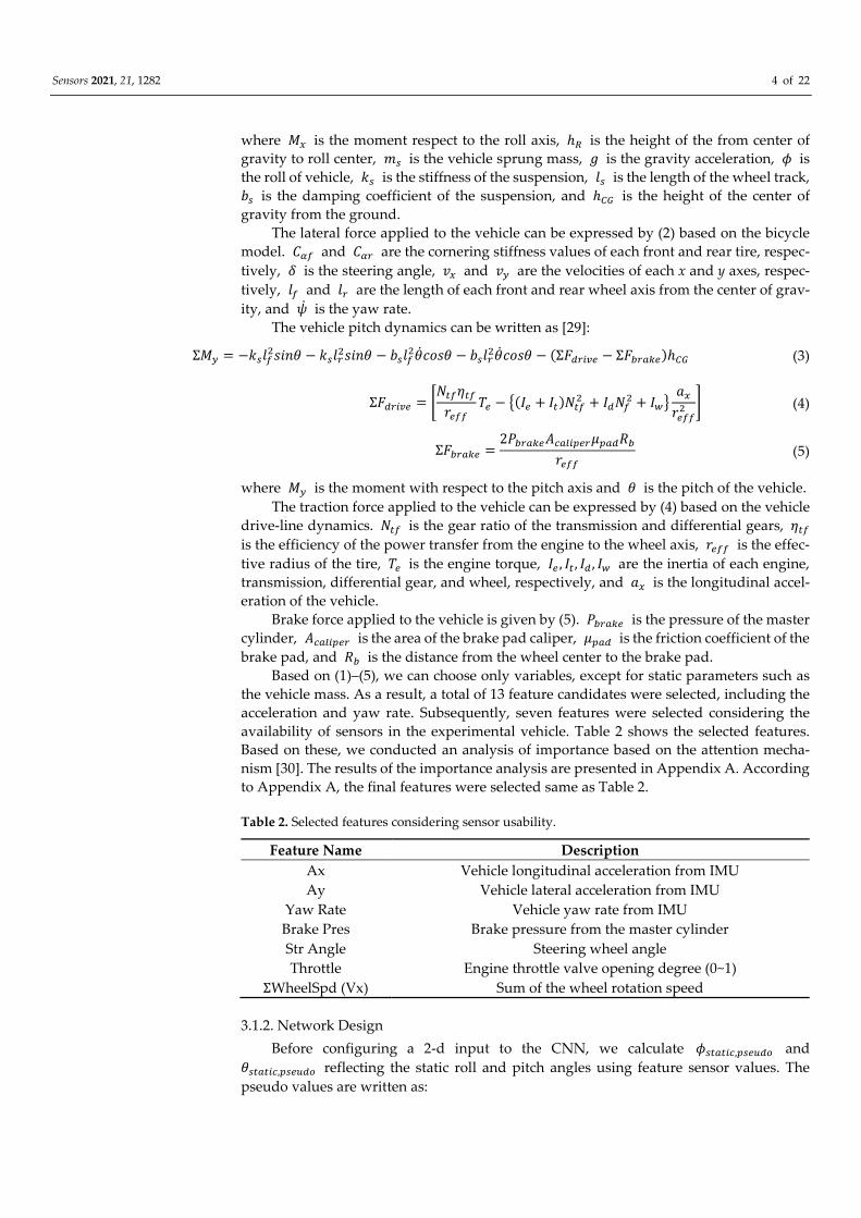
(a)

Sensors 2021, 21, 1282 15 of 22

(b)

(c)

(d)

Figure 9. Simulation results of Case 1. (a) Roll/pitch profile. (b) ��, �� and �̇ estimation results. (c) �̇ and �̇ estimation

results. (d) �� and �� estimation results.

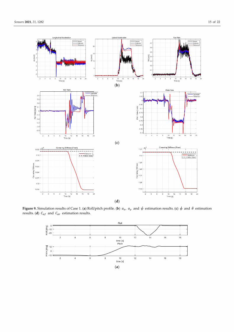
(a)

Sensors 2021, 21, 1282 16 of 22

(b)

(c)

(d)

Figure 10. Simulation results of Case 2. (a) Roll/pitch profile. (b) ��, ��, and �̇ estimation results. (c) �̇ and �̇ estimation


Sensors 2021, 21, 1282 17 of 22

(a)

(b)

(c)

(d)

Figure 11. Simulation results of Case 3. (a) Roll/pitch profile. (b) ��, ��, and �̇ estimation results. (c) �̇ and �̇ estimation


Sensors 2021, 21, 1282 18 of 22

Figure 12. Effect of cornering stiffness estimation in Case 3.

Table 7 shows the accuracy of the commercial sensor, obtained from its datasheet,

and RMSE calculation results of the estimation values for case 1–3. In case 1, there was a

fatal error of sensor value of �� due to roll angle, and case 2 exhibited considerably var-

ying roll and pitch angles; therefore, the value of �� and �� from sensors may not be

accurate. Figures 9b and 10b confirm that these errors in sensor values are successfully

corrected to obtain estimates close to the reference. In addition, in normal driving scenar-

ios, as in the 60–65 s duration in Case 3, an �� sensor error by pitch is noted, which has

also been successfully corrected. Furthermore, in all cases, filter effects that reduce noise

from existing sensors can be checked through ��, ��, and �̇. Compared with a commer-

cial sensor, �� and �� show similar accuracy, whereas �̇ shows a significantly higher

accuracy. However, in the case of commercial sensors, there may be errors caused by roll

and pitch angles; therefore, DEKF can have commercial sensor level or higher accuracy

even though correcting those errors.

The roll and pitch rates could be estimated because they were included in the state

vector, although the sensor values were not included. The roll rate accuracy was occasion-

ally lower than that of commercial sensors depending on the case, and in the case of pitch

rate, it is not comparable because there is no output of commercial sensors, but it can be

confirmed from the RMSE values that the estimated values have a fairly high accuracy.

Sensors 2021, 21, 1282 19 of 22

Table 7. RMSE calculation results of DEKF and accuracy obtained from SMI860 datasheet.

Accuracy

DEKF (RMSE) Commercial Sensor 1

�� (m/s2)

Case 1 0.4325

≤ ±0.5 Case 2 0.8075

Case 3 0.3087

�� (m/s2)

Case 1 0.8232

≤ ±0.5 Case 2 0.4204

Case 3 0.5085

�̇ (deg/s)

Case 1 0.7391

≤ ±3 Case 2 0.3953

Case 3 0.5844

�̇ (deg/s)

Case 1 5.8499

≤ ±2 Case 2 5.1394

Case 3 1.0542

�̇ (deg/s)

Case 1 1.9251

- 2 Case 2 1.7475

Case 3 0.6704 1 From SMI860 IMU datasheet of BOSCH Co., Ltd. 2 SMI860 cannot sense the pitch rate.

Figures 9d, 10d, and 11d show the estimated cornering stiffness. Figure 12 and Table

8 show the results with and without cornering stiffness estimation in Case 3, which can

improve accuracy by approximately 3–5%, particularly with a greater effect on ��.

Table 8. RMSE of with and without cornering stiffness estimation in Case 3.

RMSE

Without Cornering Stiffness Estimation With Cornering Stiffness Estimation

�� (m/s2) 0.5541 0.5085

�̇ (deg/s) 0.6131 0.5844

5. Conclusions and Future Work

In this paper, we proposed a CNN-based neural network to estimate the roll and

pitch angles of a vehicle. A DEKF was used to correct the gravitational effect caused by

the roll and pitch for estimating the exact acceleration and angular velocity.

By using the vehicle’s chassis sensor data as a time series, the neural network could

estimate the roll and pitch angles of the vehicle without a GPS or six-dimensional IMU.

Based on the estimated roll and pitch angels, we designed an extended Kalman filter

(EKF) using the 6-DOF vehicle model. Another EKF was designed, and the two EKFs were

used to estimate the cornering stiffness. We then constructed the DEKF.

Using experimental data obtained using a real car, the proposed roll and pitch esti-

mator was validated, and the DEKF was validated in the CarSim simulation environment.

The roll and pitch estimator showed an improved performance compared to the commer-

cial sensors in dynamic scenarios and also reduced the noise. However, the performance

in static scenarios was weaker. The acceleration and angular velocity estimator could ef-

fectively correct the acceleration sensor error due to roll and pitch with a de-noising effect.

In addition, the roll and pitch rates that could not be obtained from sensors could be esti-

mated with significant accuracy. By comparing the results before and after including the

cornering stiffness, we found that the accuracy is improved if the cornering stiffness is

considered.

Sensors 2021, 21, 1282 20 of 22

On the other hand, our work has limitations and challenges that should be further

discussed. We plan to consider fusion with other algorithms to improve the attitude esti-

mation performance in static scenarios. In addition, the proposed method has not been

checked in case of a change in the vehicle weight. It will also be necessary to verify the

performance of the algorithm due to changes in vehicle weight. Furthermore, our pro-

posed algorithm is hard to apply as an embedded system in vehicle because the neural

network has large capacity. The future work should be conducted to enable algorithm to

operate as real-time in vehicle through simplification and optimization.

Author Contributions: Conceptualization, M.O. and S.O.; methodology, M.O.; software, M.O.;

validation, M.O. and S.O.; formal analysis, M.O. and S.O; investigation, M.O.; resources, J.H.P.;

data curation, S.O.; writing—original draft preparation, M.O.; writing—review and editing, S.O.

and J.H.P.; visualization, M.O.; supervision, J.H.P.; project administration, S.O. and J.H.P.; funding

acquisition, J.H.P. All authors have read and agreed to the published version of the manuscript.

Funding: This work was supported by the Hyundai Motor Group Academy Industry Research

Collaboration.

Informed Consent Statement: Not applicable.

Institutional Review Board Statement: Not applicable.

Data Availability Statement: Restrictions apply to the availability of these data. Data was obtained

from Hyundai Motor Company and are available with the permission of Autonomous Driving Cen-

ter of Hyundai Motor Company R&D Division.

Acknowledgments: This work was supported by Autonomous Driving Center of Hyundai Motor

Company R&D Division.

Conflicts of Interest: The authors declare no conflict of interest.

Appendix A. Feature Importance Analysis

Figure A1. Result of feature importance weight analysis.

Table A1. Feature name of each number.

Feature Number Feature Name

1 Ax

2 Ay

3 Yaw Rate

4 Brake Pressure

5 Steering Angle

6 Engine Throttle

7 ΣWheel Speed (Vx)

All features have an importance weight higher than 0.8; therefore, feature reduction

is not performed.

Sensors 2021, 21, 1282 21 of 22

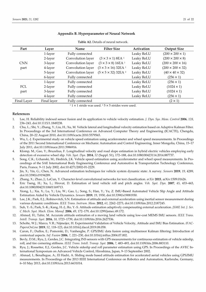
Appendix B. Hyperparameter of Neural Network

Table A2. Details of neural network.

Part Layer Name Filter Size Activation Output Size

CNN

part

1-layer Fully connected Leaky ReLU (200 × 200 × 1)

2-layer Convolution layer (3 × 3 × 1) 8EA 1 Leaky ReLU (200 × 200 × 8)




6-layer Fully connected Leaky ReLU (256 × 1)

FCL

part





Final Layer Final layer Fully connected (2 × 1) 1 1 × 1 stride was used. 2 5 × 5 strides were used.

References

1. Lee, H. Reliability indexed sensor fusion and its application to vehicle velocity estimation. J. Dyn. Sys. Meas. Control 2006, 128,

236–243, doi:10.1115/1.1849238.

2. Chu, L.; Shi, Y.; Zhang, Y.; Liu, H.; Xu, M. Vehicle lateral and longitudinal velocity estimation based on Adaptive Kalman Filter.

In Proceedings of the 3rd International Conference on Advanced Computer Theory and Engineering (ICACTE), Chengdu,

China, 20–22 August 2010, doi:10.1109/icacte.2010.5579565.

3. Wu, L.-J. Experimental study on vehicle speed estimation using accelerometer and wheel speed measurements. In Proceedings

of the 2011 Second International Conference on Mechanic Automation and Control Engineering, Inner Mongolia, China, 15–17

July 2011, doi:10.1109/mace.2011.5986916.

4. Klomp, M.; Gao, Y.; Bruzelius, F. Longitudinal velocity and road slope estimation in hybrid electric vehicles employing early

detection of excessive wheel slip. Veh. Syst. Dyn. 2014, 52 (Suppl. S1), 172–188, doi:10.1080/00423114.2014.887737.

5. Song, C.K.; Uchanski, M.; Hedrick, J.K. Vehicle speed estimation using accelerometer and wheel speed measurements. In Pro-

ceedings of the SAE International Body Engineering Conference and Automotive & Transportation Technology Conference,

Paris, France, 9–11 July 2002, doi:10.4271/2002-01-2229.

6. Jin, X.; Yin, G.; Chen, N. Advanced estimation techniques for vehicle system dynamic state: A survey. Sensors 2019, 19, 4289,

doi:10.3390/s19194289.

7. Zhang, X.; Zhao, J.; LeCun, Y. Character-level convolutional networks for text classification. arXiv 2015, arXiv:1509.01626.

8. Eric Tseng, H.; Xu, L.; Hrovat, D. Estimation of land vehicle roll and pitch angles. Veh. Syst. Dyn. 2007, 45, 433–443,

doi:10.1080/00423110601169713.

9. Xiong, L.; Xia, X.; Lu, Y.; Liu, W.; Gao, L.; Song, S.; Han, Y.; Yu, Z. IMU-Based Automated Vehicle Slip Angle and Attitude

Estimation Aided by Vehicle Dynamics. Sensors 2019, 19, 1930, doi:10.3390/s19081930.

10. Lee, J.K.; Park, E.J.; Robinovitch, S.N. Estimation of attitude and external acceleration using inertial sensor measurement during

various dynamic conditions. IEEE Trans. Instrum. Meas. 2012, 61, 2262–2273, doi:10.1109/tim.2012.2187245.

11. Suh, Y.-S.; Park, S.-K.; Kang, H.-J.; Ro, Y.-S. Attitude estimation adaptively compensating external acceleration. JSME Int. J. Ser.

C Mech. Syst. Mach. Elem. Manuf. 2006, 49, 172–179, doi:10.1299/jsmec.49.172.

12. Ahmed, H.; Tahir, M. Accurate attitude estimation of a moving land vehicle using low-cost MEMS IMU sensors. IEEE Trans.

Intell. Transp. Syst. 2016, 18, 1723–1739, doi:10.1109/tits.2016.2627536.

13. Scholte, W.J.; Marco, V.R.; Nijmeijer, H. Experimental Validation of Vehicle Velocity, Attitude and IMU Bias Estimation. IFAC-

PapersOnLine 2019, 52, 118–123, doi:10.1016/j.ifacol.2019.08.058.

14. Caron, F.; Duflos, E.; Pomorski, D.; Vanheeghe, P. GPS/IMU data fusion using multisensor Kalman filtering: Introduction of

contextual aspects. Inf. Fusion 2006, 7, 221–230, doi:10.1016/j.inffus.2004.07.002.

15. Bevly, D.M.; Ryu, J.; Gerdes, J.C. Integrating INS sensors with GPS measurements for continuous estimation of vehicle sideslip,

roll, and tire cornering stiffness. IEEE Trans. Intell. Transp. Syst. 2006, 7, 483–493, doi:10.1109/tits.2006.883110.

16. Ryu, J.; Rossetter, E.J.; Gerdes, J.C. Vehicle sideslip and roll parameter estimation using GPS. In Proceedings of the AVEC In-

ternational Symposium on Advanced Vehicle Control, Hiroshima, Japan, 9–13 September 2002.

17. Ahmad, I.; Benallegue, A.; El Hadri, A. Sliding mode based attitude estimation for accelerated aerial vehicles using GPS/IMU

measurements. In Proceedings of the 2013 IEEE International Conference on Robotics and Automation, Karlsruhe, Germany,

6–10 May 2013, doi:10.1109/icra.2013.6631014.

Sensors 2021, 21, 1282 22 of 22

18. Rajamani, R.; Piyabongkarn, D.; Tsourapas, V.; Lew, J.Y. Parameter and state estimation in vehicle roll dynamics. IEEE Trans.

Intell. Transp. Syst. 2011, 12, 1558–1567, doi:10.1109/tits.2011.2164246.

19. Garcia Guzman, J.; Prieto Gonzalez, L.; Pajares Redondo, J.; Sanz Sanchez, S.; Boada, B.L. Design of Low-Cost Vehicle Roll Angle

Estimator Based on Kalman Filters and an IoT Architecture. Sensors 2018, 18, 1800, doi:10.3390/s18061800.

20. Park, M.; Yim, S. Design of Robust Observers for Active Roll Control. IEEE Access 2019, 7, 173034–173043, doi:10.1109/AC-

CESS.2019.2956743.

21. Chung, T.; Yi, S.; Yi, K. Estimation of vehicle state and road bank angle for driver assistance systems. Int. J. Automot. Technol.

2007, 8, 111–117.

22. Tseng, H.E. Dynamic estimation of road bank angle. Veh. Syst. Dyn. 2001, 36, 307–328, doi:10.1076/vesd.36.4.307.3547.

23. Oh, J.; Choi, S.B. Vehicle roll and pitch angle estimation using a cost-effective six-dimensional inertial measurement unit. Proc.

Inst. Mech. Eng. Part D: J. Automob. Eng. 2013, 227, 577–590, doi:10.1177/0954407012459138.

24. Kamal Mazhar, M.; Khan, M.J.; Bhatti, A.I.; Naseer, N. A Novel Roll and Pitch Estimation Approach for a Ground Vehicle

Stability Improvement Using a Low Cost IMU. Sensors 2020, 20, 340, doi:10.3390/s20020340.

25. Vargas-Meléndez, L.; Boada, B.L.; Boada, M.J.L.; Gauchía, A.; Díaz, V. A sensor fusion method based on an integrated neural

network and Kalman filter for vehicle roll angle estimation. Sensors 2016, 16, 1400, doi:10.3390/s16091400.

26. Vargas-Melendez, L.; Boada, B.L.; Boada, M.J.L.; Gauchia, A.; Diaz, V. Sensor Fusion based on an integrated neural network

and probability density function (PDF) dual Kalman filter for on-line estimation of vehicle parameters and states. Sensors 2017,

17, 987, doi:10.3390/s17050987.

27. González, L.P.; Sánchez, S.S.; Garcia-Guzman, J.; Boada, M.J.L.; Boada, B.L. Simultaneous Estimation of Vehicle Roll and Side-

slip Angles through a Deep Learning Approach. Sensors 2020, 20, 3679, doi:10.3390/s20133679.

28. Taehui, L.; Sang Won, Y. Estimation of Vehicle Roll and Road Bank Angle based on Deep Neural Network. In Proceedings of

the KSAE 2018 Annual Autumn Conference & Exhibition, Jeongseon, Korea, 14–17 November 2018.

29. Rajamani, R. Vehicle Dynamics and Control, 2nd ed.; Springer Science & Business Media: NY, USA, 2011.

30. Challita, N.; Khalil, M.; Beauseroy, P. New feature selection method based on neural network and machine learning. In Pro-

ceedings of the 2016 IEEE International Multidisciplinary Conference on Engineering Technology (IMCET), Beirut, Lebanon, 2–

4 November 2016, doi:10.1109/imcet.2016.7777431.

31. Yang, S.; Kim, J. Validation of the 6-dof vehicle dynamics model and its related VBA program under the constant radius turn

manoeuvre. Int. J. Automot. Technol. 2012, 13, 593–605, doi:10.1007/s12239-012-0057-9.

32. Ray, L.R. Nonlinear tire force estimation and road friction identification: Simulation and experiments. Automatica 1997, 33, 1819–

1833.

33. Lee, D.-H.; Kim, I.-K.; Huh, K.-S. Tire Lateral Force Estimation System Using Nonlinear Kalman Filter. Trans. Korean Soc. Au-

tomot. Eng. 2012, 20, 126–131, doi:10.7467/ksae.2012.20.6.126.

34. Wenzel, T.A.; Burnham, K.; Blundell, M.; Williams, R. Dual extended Kalman filter for vehicle state and parameter estimation.

Veh. Syst. Dyn. 2006, 44, 153–171, doi:10.1080/00423110500385949.

Documents

Estimation of Vehicle Attitude, Acceleration and Angular